The ground truth about metadata and community detection in networks

Leto Peel,1, 2, ∗ Daniel B. Larremore,3, † and Aaron Clauset4, 5, 3, ‡

1ICTEAM, Universite Catholique de Louvain, Louvain-la-Neuve, Belgium2naXys, Universite de Namur, Namur, Belgium3Santa Fe Institute, Santa Fe, NM 87501, USA

4Department of Computer Science, University of Colorado, Boulder, CO 80309, USA5BioFrontiers Institute, University of Colorado, Boulder, CO 80309, USA

Across many scientific domains, there is a common need to automatically extract a simplifiedview or coarse-graining of how a complex system’s components interact. This general task is calledcommunity detection in networks and is analogous to searching for clusters in independent vectordata. It is common to evaluate the performance of community detection algorithms by their abilityto find so-called ground truth communities. This works well in synthetic networks with plantedcommunities because such networks’ links are formed explicitly based on those known communities.However, there are no planted communities in real world networks. Instead, it is standard practiceto treat some observed discrete-valued node attributes, or metadata, as ground truth. Here, weshow that metadata are not the same as ground truth, and that treating them as such inducessevere theoretical and practical problems. We prove that no algorithm can uniquely solve com-munity detection, and we prove a general No Free Lunch theorem for community detection, whichimplies that there can be no algorithm that is optimal for all possible community detection tasks.However, community detection remains a powerful tool and node metadata still have value so acareful exploration of their relationship with network structure can yield insights of genuine worth.We illustrate this point by introducing two statistical techniques that can quantify the relationshipbetween metadata and community structure for a broad class of models. We demonstrate thesetechniques using both synthetic and real-world networks, and for multiple types of metadata andcommunity structure.

INTRODUCTION

Community detection is a fundamental task of networkscience that seeks to describe the large-scale structure ofa network by dividing its nodes into communities (alsocalled blocks or groups), based only on the pattern oflinks. This task is similar to that of clustering vectordata, as both seek to identify meaningful groups withinsome data set.

Community detection has been used productively inmany applications, including identifying allegiances orpersonal interests in social networks [1, 2], biologicalfunction in metabolic networks [3, 4], fraud in telecom-munications networks [5], and homology in genetic simi-larity networks [6]. Many approaches to community de-tection exist, spanning not just different algorithms andpartitioning strategies, but also fundamentally differentdefinitions of what it means to be a “community.” Thisdiversity is a strength, as networks generated by differentprocesses and phenomena should not a priori be expectedto be well-described by the same structural principles.

With so many different approaches to community de-tection available, it is natural to compare them to as-sess their relative strengths and weaknesses. Typically,this comparison is made by assessing a method’s abil-ity to identify so-called ground truth communities, a sin-

∗ Contributed equally; leto.peel@uclouvain.be† Contributed equally; larremore@santafe.edu‡ aaron.clauset@colorado.edu

gle partition of the network’s nodes into groups which isconsidered the correct answer. This approach for eval-uating community detection methods works well in ar-tificially generated networks, whose links are explicitlyplaced according to those ground truth communities anda known data generating process. For this reason, thepartition of nodes into ground truth communities in syn-thetic networks is called a planted partition. However,for real-world networks, both the correct partition andthe true data generating process are typically unknown,which necessarily implies that there can be no groundtruth communities for real networks. Without access tothe very thing these methods are intended to find, objec-tive evaluation of their performance is difficult.

Instead, it has become standard practice to treat someobserved data on the nodes of a network, which we callnode metadata, (e.g., a person’s ethnicity, gender or af-filiation for a social network, or a gene’s functional classfor a gene regulatory network) as if they were groundtruth communities. While this widespread practice isconvenient, it can lead to incorrect scientific conclusionsunder relatively common circumstances. In this paper,we identify these consequences and articulate the episte-mological argument against treating metadata as groundtruth communities. Next, we provide rigorous mathe-matical arguments and prove two theorems that renderthe search for a universally best ground-truth recoveryalgorithm as fundamentally flawed. We then present twonovel methods that can be used to productively explorethe relationship between observed metadata and com-munity structure, and demonstrate both methods on avariety of synthetic and real-world networks, using mul-

arX

iv:1

608.

0587

8v2

[cs

.SI]

3 M

ay 2

017

2

tiple community detection frameworks. Through theseexamples, we illustrate how a careful exploration of therelationship between metadata and community structurecan shed light on the role that node attributes play ingenerating network links in real complex systems.

RESULTS

The trouble with metadata and communitydetection

The use of node metadata as a proxy for ground truthstems from a reasonable need: since artificial networksmay not be representative of naturally occurring net-works, community detection methods must also be con-fronted with real-world examples to show that they workwell in practice. If the detected communities correlatewith the metadata, we may reasonably conclude that themetadata are involved in or depend upon the generationof the observed interactions. However, the scientific valueof a method is as much defined by the way it fails as byits ability to succeed. Because metadata always havean uncertain relationship with ground truth, failure tofind a good division that correlates with our metadata isa highly confounded outcome, arising for any of severalreasons:

(i) these particular metadata are irrelevant to thestructure of the network,

(ii) the detected communities and the metadata cap-ture different aspects of the network’s structure,

(iii) the network contains no communities as in a simplerandom graph [7] or a network that is sufficientlysparse that its communities are not detectable [8],or

(iv) the community detection algorithm performedpoorly.

In the above, we refer to the observed network and meta-data and note that noise in either could lead to one of thereasons above. For instance, measurement error of thenetwork structure may make our observations unreliableand in extreme cases can obscure community structureentirely, resulting in case (iii). It is also possible thathuman errors are introduced when handling the data,exemplified by the widely used American college footballnetwork [9] of teams that played each other in one season,whose associated metadata representing each team’s con-ference assignment were collected during a different sea-son [10]. Large errors in the metadata can render themirrelevant to the network [case (i)].

Most work on community detection assumes that fail-ure to find communities that correlate with metadata im-plies case (iv), algorithm failure, although some criticalwork has focused on case (iii), difficult or impossible torecover communities. The lack of consideration for cases(i) and (ii) suggests the possibility for selection bias in

-240

-230

-220

-210

SB

M lo

g lik

elih

ood

-200

partition space

FIG. 1. The stochastic blockmodel (SBM) log-likelihood sur-face for bipartitions of the Karate Club network [14]. Thehigh-dimensional space of all possible bipartitions of the net-work has been projected onto the x, y-plane (using a methoddescribed in Supplementary Text D 4) such that points repre-senting similar partitions are closer together. The surfaceshows two distinct peaks that represent scientifically rea-sonable partitions. The lower peak corresponds to the so-cial group partition given by the metadata—often treated asground truth—while the higher peak corresponds to a leader-follower partition.

the published literature in this area (a point recently sug-gested by [11]). Indeed, recent critiques of the generalutility of community detection in networks [11–13] canbe viewed as a side effect of confusion about the role ofmetadata in evaluating algorithm results.

For these reasons, using metadata to assess the per-formance of community detection algorithms can lead toerrors of interpretation, false comparisons between meth-ods, and oversights of alternative patterns and expla-nations, including those that do not correlate with theknown metadata.

For example, Zachary’s Karate Club [14] is a small real-world network with compelling metadata frequently usedto demonstrate community detection algorithms. Thenetwork represents the observed social interactions of 34members of a karate club. At the time of study, the clubfell into a political dispute and split into two factions.These faction labels are the metadata commonly usedas ground truth communities in evaluating communitydetection methods. However, it is worth noting at thispoint that Zachary’s original network and metadata differfrom those commonly used for community detection [9].Links in the original network were by the different typesof social interaction that Zachary observed. Zachary alsorecorded two metadata attributes: the political leaningof each of the members (strong, weak, or neutral supportfor one of the factions) and the faction they ultimatelyjoined after the split. However, the community detectionliterature uses only the metadata representing the factioneach node joined, often with one of the nodes mislabeled.

3

This node (“Person number 9”) supported the presidentduring the dispute but joined the instructor’s faction asjoining the president’s faction would have involved re-training as a novice when he was only two weeks awayfrom taking his black belt exam.

The division of the Karate Club nodes into factions isnot the only scientifically reasonable way to partition thenetwork. Figure 1 shows the log-likelihood landscape fora large number of two-group partitions (embedded in twodimensions for visualization) of the Karate Club, underthe stochastic blockmodel (SBM) for community detec-tion [15, 16]. Partitions that are similar to each other areembedded nearby in the horizontal coordinates, mean-ing that the two broad peaks in the landscape representtwo distinct sets of high-likelihood partitions, one cen-tered around the faction division and one that dividesthe network into leaders and followers. Other commonapproaches to community detection [9, 17], suggest thatthe best divisions of this network have more than twocommunities [10, 18]. The multiplicity and diversity ofgood partitions illustrates the ambiguous status of thefaction metadata as a desirable target.

The Karate Club network is among many examplesfor which standard community detection methods re-turn communities that either subdivide the metadatapartition [19] or do not correlate with the metadata atall [20, 21]. More generally, most real-world networkshave many good partitions and there are many plausibleways to sort all partitions to find good ones, sometimesleading to a large number of reasonable results. More-over, there is no consensus on which method to use onwhich type of network [21, 22].

In what follows, we explore both the theoretical ori-gins of these problems and the practical means to ad-dress the confounding cases described above. To do so,we make use of a generative model perspective of commu-nity detection. In this perspective, we describe the rela-tionship between community assignements C and graphsG via a joint distribution P (C,G) over all possible com-munity assignments and graphs that we may observe.We take this perspective because it provides a preciseand interpretable description of the relationship betweencommunities and network structure. Although genera-tive models, like the SBM, describe the relationship be-tween networks and communities directly via a mathe-matically explicit expression for P (C,G), other methodsfor community detection nevertheless maintain an im-plicit relationship between network structure and com-munity assignment. As such, the theorems we present,as well as their implications are more generally applicableacross all methods of community detection.

In the next section we present rigorous theoretical re-sults with direct implications for cases (i) and (iv), whilethe remaining sections introduce two statistical meth-ods for addressing cases (i) and (ii), respectively. Thesecontributions do not address case (iii), when there is nostructure to be found, which has been previously exploredby other authors, e.g., for the SBM [8, 23–27] and mod-

ularity [28, 29].

Ground truth and metadata in community detection

Community detection is an inverse problem: using onlythe edges of the network as data, we aim to find thegrouping or partition of the nodes that relates to how thenetwork came to be. More formally, suppose that somedata generating process g embeds ground-truth commu-nities T in the patterns of links in a network G = g(T ).Our goal is to discover those communities based only onthe observed links. To do so, we write down a communitydetection scheme f that uses the network to find commu-nities C = f(G). If we have chosen f well, then the com-munities C will be equal to the ground truth T and wehave solved the inverse problem. Thus, the communitydetection problem for a single network seeks a method f∗

that minimizes the distance between the identified com-munities and the ground truth:

f∗ = arg minf

d(T , f(G)) , (1)

where d is a measure of distance between partitions.For a method f to be generally useful, it should be the

minimizer for many different graphs, each with its owngenerative process and ground truth. Often in the com-munity detection literature, several algorithms are testedon a range of networks to identify which performs bestoverall [12, 30, 31]. If a universally optimal communitydetection method exists, it must solve Eq. (1) for anytype of generative process g and partition T , that is,

∃ f∗ s.t. f∗ = arg minf

d(T , f (g(T ))

)∀g, T . (2)

In fact, no such universal f∗ community detectionmethod can exist because the mapping from generativemodels g and ground truth partitions T to graphs Gis not uniquely invertible due to the fact that the mapis not a bijection. In other words, any particular net-work G can be produced by multiple, distinct genera-tive processes, each with its own ground truth, such thatG = g1(T1) = g2(T2), with (g1, T1) 6= (g2, T2). Thus,no community detection algorithm method can uniquelysolve the problem for all possible networks (Eq. (2)), oreven a single network (Eq. (1)). This reasoning under-pins the following theorem, which we state and prove inSupplementary Text C:

Theorem 1: For a fixed network G, the so-lution to the ground truth community de-tection problem—given G, find the T suchthat G = g(T )—is not unique.

Substituting metadata M for ground truth T exacer-bates the situation by creating additional problems. Inreal networks we do not know the ground truth or thegenerating process. Instead, it is common to seek a par-tition that matches some node metadataM. Optimizing

4

a community detection method to discover M is equiva-lent to finding f∗ such that

f∗ = arg minf

d(M, f(G)) , (3)

yet this does not necessarily solve the community detec-tion problem of Eq. (1) since we cannot guarantee thatthe metadata are equivalent to the unobserved groundtruth, d(M, T ) = 0. Consequently, both d(C, T ) = 0and d(C, T ) > 0 are possibilities. Thus, when we evalu-ate a community detection method by its ability to finda metadata partition, we confound the metadata’s cor-respondence to the true communities, i.e., d(M, T ) [case(ii) in the previous section] and the community detectionmethod’s ability to find true communities, i.e., d(C, T )[case (iv)]. In this way, treating metadata as groundtruth simultaneously tests the metadata’s relevance andthe algorithm’s performance, with no ability to differen-tiate between the two. For instance, when consideringcompeting partitions of the Karate Club (Figure 1), theleader-follower partition is the most likely partition underthe SBM, yet it correlates poorly with the known meta-data. On the other hand, under the degree-correctedSBM, the optimal partition is more highly correlatedwith the metadata (Fig. S1). Based only on the perfor-mance of recovering metadata, one would conclude thatthe degree-corrected model is better. However, if Zacharyhad not provided the faction information, but insteadsome metadata that correlated with the degree (e.g. theidentities of the club’s four officers) then our conclusionmight change to the regular SBM being the better model.We would arrive at a different conclusion despite the factthat the network, and the underlying process that gener-ated it, remain unchanged. A similar case of dependenceon a particular choice of metadata are exemplified bydivisions of high-school social networks using metadataof students’ grade level or race [21]. Past evaluations ofcommunity detection algorithms that only measure per-formance by metadata recovery are thus inconclusive. Itis only with synthetic data, where the generative processis known, that ground truth is knowable and performanceobjectively measurable.

However, even when the generative process is knownfor a single network or even a set of networks, there isno best community detection method over all networks.This is because, when averaged over all possible commu-nity detection problems, every algorithm has provablyidentical performance, a notion that is captured in a NoFree Lunch theorem for community detection which werigorously state and prove in Supplementary Text C andparaphrase here:

Theorem 3 (paraphrased): For thecommunity detection problem, with accu-racy measured by adjusted mutual infor-mation, the uniform average of the accu-racy of any method f over all possible com-munity detection problems is a constantwhich is independent of f .

This No Free Lunch theorem, based on the No FreeLunch theorems for supervised learning [32], implies thatno method has an a priori advantage over any otheracross all possible community detection tasks. (In fact,Theorem 3 and its proof apply to clustering and par-titioning methods in general, beyond community detec-tion.) In other words, for a set of cases that a particularmethod fa outperforms fb, there must exist a set of caseswhere fb outperforms fa—on average no algorithm per-forms better than any other. Yet this does not rendercommunity detection pointless because the theorem alsoimplies that if the tasks of interest correspond to a re-stricted subset of cases (e.g., finding communities in generegulatory networks or certain kinds of groups in socialnetworks), then there may indeed be a method that out-performs others within the confines of that subset. Inshort, matching beliefs about the data generating pro-cess g with the assumptions of the algorithm f can leadto better and more accurate results, at the cost of re-duced generalizability. (See Supplementary Text C foradditional discussion.)

The combined implications of the epistemological ar-guments in the previous section with Theorems 1 and 3in this section do not render community detection impos-sible or useless, by any means. They do, however, implythat efforts to find a universally best community detec-tion algorithm are in vain, and that metadata should notbe used as a benchmark for evaluating or comparing theefficacy of community detection algorithms. These the-orems indicate that better community detection resultsmay stem from a better understanding of how to dividethe problem space into categories of community detectiontasks, eventually identifying classes of algorithms whosestrengths are aligned with the requirements of a specificcategory.

Relating metadata and structure

From a scientific perspective, metadata labels have di-rect and genuine value in helping to understand complexsystems. Metadata describe the nodes, while communi-ties describe how nodes interact. Therefore, correspon-dence between metadata and communities suggests a re-lationship between how nodes interact and the propertiesof the nodes themselves. This correspondence has beenused productively to assist in the inference of communitystructure [21], learn the relationship between metadataand network topology [33, 34] and explain dependenciesbetween metadata and network structure [35].

Here we propose two new methods to explore howmetadata relate to the structure of the network whenthe metadata only correlate weakly with the identifiedcommunities. Both methods utilize the powerful tools ofprobabilistic models, but are not restricted to any partic-ular model of community structure. The first method is astatistical test to assess whether or not the metadata par-tition and network structure are related [case (i)]. The

5

second method explores the space of network partitionsto determine if the metadata represent the same or dif-ferent aspects of the network structure as the “optimal”communities inferred by a chosen model [case (ii)].

In principle, any probabilistic generative model(e.g., [15, 16, 36–39]) of communities in networks couldbe used within these methods. Here we derive results forthe popular stochastic blockmodel [15, 16] and its degree-corrected version [20] (alternative formulations discussedin Supplementary Texts B and A). The SBM defines com-munities as sets of nodes that are stochastically equiva-lent. This means that the probability pij of a link be-tween a pair of nodes i and j depends only on theircommunity assignment, i.e., pij = ωπi,πj

, where πi isthe community assignment for node i and ωπi,πj

is theprobability that a link exists between members of groupsπi and πj . This general definition of community struc-ture is quite flexible, and allows for both assortative anddisassortative community structure, as well as arbitrarymixtures thereof.

Testing for a relationship between metadata andstructure

Our first method, called the blockmodel entropy signif-icance test (BESTest), is a statistical test to determine ifthe metadata partition is relevant to the network struc-ture [case (i)], i.e., if it provides a good description ofthe network under a given model. We quantify relevanceusing the entropy, which is a measure of how many bitsof information it takes to record the network given boththe network model and its parameters. The lower theentropy under this model, the better the metadata de-scribe the network, while a higher entropy implies thatthe metadata and the patterns of edges in the networkare relatively uncorrelated. We derive and discuss theBESTest using five different models in SupplementaryText B. Here we describe a particularly straightforwardversion of this test using the SBM.

The BESTest works by first dividing a network’s nodesaccording to the labels of the metadata and then com-puting the entropy of the SBM that best describes thepartitioned nodes. This entropy is then compared to adistribution of entropies using the same network but ran-dom permutations of the metadata labels, resulting in astandard p-value. Specifically, we use the SBM with max-imum likelihood parameters for the partition induced bythe metadata, which is given by ωrs = mrs

nrnswhere mrs is

the number of links between group r and group s and nris the number of nodes in group r. Then we compute theentropy H(G;M), which we derive and discuss in detail,along with derivations of entropies for other models, inSupplementary Text B.

The statistical significance of the entropy valueH(G;M) is obtained by comparing it to the entropyof the same network but randomly permuted metadata.Specifically, we compute a null distribution of such val-

ues, derived by calculating the entropies induced by ran-dom permutations π of the observed metadata valuesH(G; π). This choice of null model preserves both theempirical network structure and the relative frequenciesof metadata values, but removes the correlation betweenthe two. The result is a standard p-value, defined as

p-value = Pr [H(G; π) ≤ H(G;M)] , (4)

which can be estimated empirically by computingH(G; π) for a large number of randomly permuted meta-data vectors π. Smaller p-values indicate that the meta-data provide a better description of the network, makingit relatively less plausible that a random permutation ofthe metadata values could describe the network as well asthe observed metadata does. It is important to note thatp-values measure statistical significance but not effectstrength, meaning that a low p-value does not indicatea strong correlation between the metadata and the net-work structure. Recently, Bianconi et al. [40] proposeda related entropy test for this task, based on a Normalapproximation to the null distribution under the SBM.The blockmodel entropy significance test described hereis a generalization of Bianconi et al.’s test that is bothmore flexible, as it can be used with any number of nullmodels, and more accurate, as the true null distributionis substantially non-Normal (Fig. S5).

The blockmodel entropy significance test is, by con-struction, sensitive to even low correlations betweenmetadata and network structure. To quantify the sen-sitivity of this p-value, we first apply it to syntheticnetworks with known community structure (see Supple-mentary Text B for a complete description of syntheticnetwork generation). For these networks, our ability todetect relevant metadata is determined jointly by thestrength of the planted communities and the correlationbetween metadata and communities. Figure 2 shows thatfor networks with strong community structure we can re-liably detect relevant metadata even for relatively lowlevels of correlation with the planted structure. In fact,our method can still identify relevant metadata when thecommunity structure is sufficiently weak that communi-ties are provably undetectable by any community detec-tion algorithm that relies only on the network [8]. Statis-tical significance requires an increasing level of correla-tion with the underlying structure as community strengthdecreases; if there is no structure in the network (ε = 1)then any metadata partition will be correctly identifiedas irrelevant. Note that a low p-value does not mean thatthe metadata provide the best description of the network,nor does it imply that we should be able to recover themetadata partition using community detection.

We now apply the blockmodel entropy significancetest to a social network of interactions within a lawfirm, and to biological networks representing similari-ties among genes in the human malaria parasite P. fal-ciparum (see Supplementary Text D). The first set, theLazega Lawyers networks, comprises three networks onthe same set of nodes and five metadata attributes. The

6

FIG. 2. Expected p-value estimates of the blockmodel entropysignificance test as the correlation ` between metadata andplanted communities increases (each metadata label correctlyreflects the planted community with probability (1+ `)/2; seeSupplementary Text B). Each curve represents networks witha fixed community strength ε = ωrs/ωrr. Solid lines indicatestrong community structure in the so-called detectable regime(ε < λ), while dashed lines represent weak undetectable com-munities (ε > λ) [8]. Three block density diagrams visuallydepict ε values.

TABLE I. BESTest p-values for Lazega Lawyers

Metadata Attribute

Network Status Gender Office Practice Law School

Friendship < 10−6 0.034 < 10−6 0.033 0.134

Cowork < 10−3 0.094 < 10−6 < 10−6 0.922

Advice < 10−6 0.010 < 10−6 < 10−6 0.205

TABLE II. BESTest p-values for Malaria var genes

var Gene Network Number

1 2 3 4 5 6 7 8 9

Genome 0.566 0.064 0.536 0.588 0.382 0.275 0.020 0.464 0.115

multiple combinations of edge and metadata types thatyield highly significant p-values (Table I; see Table S3 forresults using additional models of community structure)indicate that each set of metadata provides non-trivial in-formation about the structure of multiple networks, andvice versa, implying that all metadata sets are relevantto the edge formation process, so none should be individ-ually treated as ground truth.

The second set, the malaria var gene networks, com-prises nine networks on the same set of nodes and threesets of metadata. For each network, we find a non-significant p-value when the metadata denote the parasitegenome-of-origin (Table II; see Table S4 for results usingadditional models of community structure and additionalmetadata). In contrast to the Lazega Lawyers network,these genome metadata are statistically irrelevant for ex-plaining the observed patterns of gene recombinations.This finding substantially strengthens the conclusions ofRef. [41] which used a less sensitive test based on labelassortativity. Some metadata for these networks do cor-

relate, however (see Supplementary Text B).

Diagnosing the structural aspects captured bymetadata and communities

Our second method provides a direct means to diag-nose whether some metadata and a network’s detectedcommunities differ because they reveal different aspectsof the network’s structure [case (ii)]. We accomplishthis by extending the SBM to probe the local struc-ture around and between the metadata partition and thedetected structural communities. This extended model,which we call the neoSBM, performs community detec-tion under a constraint in which each node is assigned oneof two states, which we call blue or red, and a parameterq that governs the number of nodes in each state. If anode is blue, its community is fixed as its metadata label,while if it is red, its community is free to be chosen by themodel. We choose q automatically within the inferencestep of the model by imposing a likelihood penalty in theform of a Bernoulli prior with parameter θ, which controlsfor the additional freedom that comes from varying q.The neoSBM’s log likelihood is LneoSBM = LSBM+qψ(θ),where ψ(θ) may be interpreted as the cost of freeing anode from its metadata label (see Supplementary Text Afor exact formulation).

By varying the cost of freeing a node, we can use theneoSBM to produce a graphical diagnostic of the inte-rior of the space between the metadata partition and theinferred community partition. In this way, the neoSBMcan shed light on how the metadata and inferred com-munity partitions are related, beyond direct comparisonof the partitions via standard techniques such as normal-ized mutual information or the Rand index. As the costof freeing nodes is reduced, the neoSBM creates a paththrough the space of partitions from metadata to theoptimal community partition and, as it does so, we mon-itor the improvement of the partition by the increase inSBM log likelihood. A steady increase indicates that theneoSBM is incrementally refining the metadata partitionuntil it matches the globally optimal SBM communities.This behavior implies that the metadata and communitypartitions represent related aspects of the network struc-ture. On the other hand, if the SBM likelihood remainsconstant for a substantial range of θ, followed by a sharpincrease or jump, it indicates that the neoSBM has movedfrom one local optimum to another. Multiple plateausand jumps indicate that several local optima have beentraversed, revealing that the partitions are capturing dif-ferent aspects of the network’s structure.

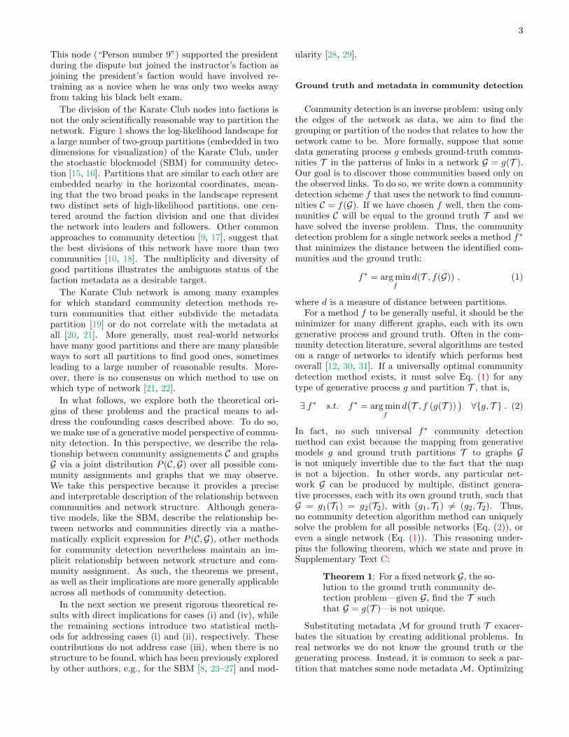
To demonstrate the usage of the neoSBM, we exam-ine the path between partitions for a synthetic networkwith four locally optimal partitions which correspond tothe four distinct peaks in the surface plot (Fig. 3A; seeSupplementary Text A for a complete description of syn-thetic network generation). We take the partition of thelowest of these peaks as metadata and use the neoSBM

7

-9

-8.5

-1500

-8

-7.5

-1000

-7

# 104

-6.5

-6

-5000 15001000500500 0-500-10001000 -1500-2000

1 2

3 41

2 3

4

1

2 34

free

node

s, q

SB

M lo

g lik

elih

ood

SB

M lo

g lik

elih

ood

A B C

FIG. 3. The neoSBM on synthetic data. (A) The stochastic block model (SBM) likelihood surface shows four distinct peakscorresponding to a sequence of locally optimal partitions. (B) Block density diagrams depict community structure for locallyoptimal partitions, where darker color indicates higher probability of interaction. (C) The neoSBM, with partition 1 as themetadata partition, interpolates between partition 1 and the globally optimal SBM partition 4. The number of free nodes qand SBM log likelihood as a function of θ show three discontinuous jumps as the neoSBM traverses each of the locally optimalpartitions (1–4).

to generate a path to the globally optimal partition byvarying the θ parameter of the neoSBM from 0 to 1.The corresponding changes in the SBM log likelihood andthe number of free nodes show three discontinuous jumps(Fig. 3C), one for each time the model encounters a newlocally optimal partition.

Examining the partitions along the neoSBM’s pathcan provide direct insights into the relationship betweenmetadata and network structure. Figure 3B shows thestructure at each of the four traversed optima as block-wise interaction matrices ω. Each partition has a dif-ferent type of large-scale structure, from core-peripheryto assortative patterns. In this way, when metadata donot closely match inferred communities, the neoSBM canshed light on whether and how the metadata capture sim-ilar or different aspects of network structure.

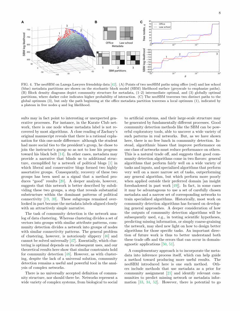
We now present an application of the neoSBM to theLazega Lawyers data analyzed in the previous section.When initialized with the law school and office locationmetadata, the neoSBM produces distinct patterns of re-laxation to the global optimum (Fig. 4A,C), approachingit from opposite sides of the peak in the likelihood sur-face. Starting at the law school metadata, the model tra-verses the space of partitions to the global SBM-optimalpartition without encountering any local optima. In con-trast, the path from the office metadata crosses one lo-cal optimum (Fig. 4A,B), which indicates that the lawschool metadata are more closely associated with thelarge-scale organization of the network than are the of-fice metadata. Both sets of metadata labels are relevant,however, as we determined in the previous section us-ing the BESTest. Results for other real-world networksare included in Supplementary Text A, including gener-alizations of the neoSBM to other community detectionmethods.

DISCUSSION

Treating node metadata as ground truth communi-ties for real-world networks is commonly justified viaan erroneous belief that the purpose of community de-tection is to recover groups that match metadata la-bels [11, 13, 31, 43]. Consequently, metadata recoveryis often used to measure community detection perfor-mance [44] and metadata are often referred to as groundtruth [21, 45]. However, the organization of real networkstypically correlates with multiple sets of metadata, bothobserved and unobserved. Thus, labeling any particu-lar set to be “ground truth” is an arbitrary and gen-erally unjustified decision. Furthermore, when a com-munity detection algorithm fails to identify communi-ties that match known metadata, poor algorithm per-formance is indistinguishable from three alternative pos-sibilities: (i) the metadata are irrelevant to the networkstructure, (ii) the metadata and communities capture dif-ferent aspects of the network structure, or (iii) the net-work lacks group structure. Here, we have introducedtwo new statistical tools to directly investigate cases (i)and (ii), while (iii) remains well addressed by work fromother authors [8, 23–29]. We have also articulated multi-ple mathematical arguments which conclude that treat-ing metadata as ground truth in community detectioninduces both theoretical and practical problems. How-ever, we have also shown that metadata remain usefuland that a careful exploration of the relationship betweennode metadata and community structure can yield newinsights into the network’s underlying generating process.

By searching only for communities that are highly cor-related with metadata, we risk focusing only on positivecorrelations while overlooking other scientifically relevantorganizational patterns. In some cases, disagreementsbetween metadata labels and community detection re-

8

Law schoolOf ficeMetadata

SBM partitions1 2 3

-900

-850

-800

-750

50

-700

0

-50-50 050100

12

3

12 3

free

node

s, q

SB

M lo

g lik

elih

ood

SB

M lo

g lik

elih

ood

A B C

FIG. 4. The neoSBM on Lazega Lawyers friendship data [42]. (A) Points of two neoSBM paths using office (red) and law school(blue) metadata partitions are shown on the stochastic block model (SBM) likelihood surface (greyscale to emphasize paths).(B) Block density diagrams depict community structure for metadata, (1–2) intermediate optimal, and (3) globally optimalpartitions, where darker color indicates higher probability of interaction. (C) The neoSBM traverses two distinct paths to theglobal optimum (3), but only the path beginning at the office metadata partition traverses a local optimum (1), indicated bya plateau in free nodes q and log likelihood.

sults may in fact point to interesting or unexpected gen-erative processes. For instance, in the Karate Club net-work, there is one node whose metadata label is not re-covered by most algorithms. A close reading of Zachary’soriginal manuscript reveals that there is a rational expla-nation for this one-node difference: although the studenthad more social ties to the president’s group, he chose tojoin the instructor’s group so as not to lose his progresstoward his black belt [14]. In other cases, metadata mayprovide a narrative that blinds us to additional struc-ture, exemplified by a network of political blogs [1] inwhich liberal and conservative blogs formed two highlyassortative groups. Consequently, recovery of these twogroups has been used as a signal that a method pro-duces “good” results [20]. A deeper analysis, however,suggests that this network is better described by subdi-viding these two groups, a step that reveals substantialsubstructure within the dominant patterns of politicalconnectivity [19, 39]. These subgroups remained over-looked in part because the metadata labels aligned closelywith an attractively simple narrative.

The task of community detection is the network ana-log of data clustering. Whereas clustering divides a set ofvectors into groups with similar attribute patterns, com-munity detection divides a network into groups of nodeswith similar connectivity patterns. The general problemof clustering, however, is notoriously slippery [46] andcannot be solved universally [47]. Essentially, which clus-tering is optimal depends on its subsequent uses, and ourtheoretical results here show that similar constraints holdfor community detection [48]. However, as with cluster-ing, despite the lack of a universal solution, communitydetection remains a useful and powerful tool in the anal-ysis of complex networks.

There is no universally accepted definition of commu-nity structure, nor should there be. Networks represent awide variety of complex systems, from biological to social

to artificial systems, and their large-scale structure maybe generated by fundamentally different processes. Goodcommunity detection methods like the SBM can be pow-erful exploratory tools, able to uncover a wide variety ofsuch patterns in real networks. But, as we have shownhere, there is no free lunch in community detection. In-stead, algorithmic biases that improve performance onone class of networks must reduce performance on others.This is a natural trade off, and suggests that good com-munity detection algorithms come in two flavors: generalalgorithms that perform fairly well on a wide variety oftasks and inputs, and specialized algorithms that performvery well on a more narrow set of tasks, outperformingany general algorithm, but which perform more poorlywhen applied outside their preferred domain [an insightforeshadowed in past work [49]]. In fact, in some casesit may be advantageous to use a set of carefully chosenmetadata and a narrow set of corresponding networks totrain specialized algorithms. Historically, most work oncommunity detection algorithms has focused on develop-ing general approaches. A deeper consideration of howthe outputs of community detection algorithms will besubsequently used, e.g., in testing scientific hypotheses,predicting missing information, or simply coarse-grainingthe network, may shed new light on how to design betteralgorithms for those specific tasks. An important direc-tion of future work is thus to better understand boththese trade offs and the errors that can occur in domain-agnostic applications [50, 51].

A complementary approach is to incorporate the meta-data into inference process itself, which can help guidea method toward producing more useful results. TheneoSBM introduced here is one such method. Oth-ers include methods that use metadata as a prior forcommunity assignment [21] and identify relevant com-munities to predict missing network or metadata infor-mation [33, 34, 52]. However, there is potential to go

9

further than these domain-agnostic methods can takeus. Tools that incorporate correct domain-specific knowl-edge about the systems they represent will provide thebest lens for revealing patterns beyond what is alreadyknown and ultimately lead to important scientific break-throughs. By rigorously probing these relationships wecan move past the false notion of metadata as groundtruth, and instead uncover the particular organizing prin-ciples underlying real world networks and their meta-data.

ACKNOWLEDGEMENTS

The authors thank Cris Moore, Tiago Peixoto, MichaelSchaub, David Wolpert, and Johan Ugander for insight-ful conversations. This work was supported by IAP(Belgian Scientific Policy Office) and ARC (FederationWallonia-Brussels) (LP), the SFI Omidyar Fellowship(DBL), and NSF Grant IIS-1452718 (AC).

DATA AND CODE

Computer code implementing the analysis methodsdescribed in this paper and other information can befound online at https://piratepeel.github.io/code.htmland http://danlarremore.com/metadata.

[1] Lada A Adamic and Natalie Glance, “The political blo-gosphere and the 2004 US election: divided they blog,” inProc. of the 3rd Int. Workshop on Link Discovery (ACM,2005) pp. 36–43.

[2] Santo Fortunato, “Community detection in graphs,”Physics Reports, 486, 75–174 (2010).

[3] Petter Holme, Mikael Huss, and Hawoong Jeong, “Sub-network hierarchies of biochemical pathways,” Bioinfor-matics, 19, 532–538 (2003).

[4] Roger Guimera and Luıs A Nunes Amaral, “Functionalcartography of complex metabolic networks,” Nature,433, 895–900 (2005).

[5] Corinna Cortes, Daryl Pregibon, and Chris Volin-sky, “Communities of interest,” in Advances in Intel-ligent Data Analysis, Lecture Notes in Computer Sci-ence, Vol. 2189, edited by Frank Hoffmann, David Hand,Niall Adams, Douglas Fisher, and Gabriela Guimaraes(Springer Berlin / Heidelberg, 2001) pp. 105–114.

[6] Leanne S Haggerty, Pierre-Alain Jachiet, William P Han-age, David A Fitzpatrick, Philippe Lopez, Mary J OCon-nell, Davide Pisani, Mark Wilkinson, Eric Bapteste, andJames O McInerney, “A pluralistic account of homology:adapting the models to the data,” Mol. Biol. Evol., 31,501–516 (2014).

[7] Paul Erdos and Alfred Renyi, “On random graphs,” Publ.Math. Debrecen, 6, 290–297 (1959).

[8] Aurelien Decelle, Florent Krzakala, Cristopher Moore,and Lenka Zdeborova, “Inference and phase transitionsin the detection of modules in sparse networks,” Phys.Rev. Lett., 107, 065701 (2011).

[9] Michelle Girvan and Mark EJ Newman, “Communitystructure in social and biological networks,” Proc. Natl.Acad. Sci. USA, 99, 7821–7826 (2002).

[10] T S Evans, “Clique graphs and overlapping communi-ties,” J. Stat. Mech.: Theory Exp., 2010, P12037 (2010).

[11] Darko Hric, Richard K Darst, and Santo Fortunato,“Community detection in networks: Structural commu-nities versus ground truth,” Phys. Rev. E, 90, 062805(2014).

[12] Jure Leskovec, Kevin J Lang, and Michael Mahoney,“Empirical comparison of algorithms for network com-munity detection,” in Proc. of the 19th Int. World Wide

Web Conf. (ACM, 2010) pp. 631–640.[13] Jaewon Yang and Jure Leskovec, “Community-affiliation

graph model for overlapping network community detec-tion,” in Proc. of the 12th Int. Conf. on Data Mining(IEEE, 2012) pp. 1170–1175.

[14] Wayne W Zachary, “An information flow model for con-flict and fission in small groups,” J. Anthropol. Res., 452–473 (1977).

[15] Paul W Holland, Kathryn Blackmond Laskey, andSamuel Leinhardt, “Stochastic blockmodels: Firststeps,” Social networks, 5, 109–137 (1983).

[16] Krzysztof Nowicki and Tom A B Snijders, “Estimationand prediction for stochastic blockstructures,” J. Amer-ican Statistical Association, 96, 1077–1087 (2001).

[17] Jianbo Shi and Jitendra Malik, “Normalized cuts and im-age segmentation,” IEEE Transactions on Pattern Anal-ysis and Machine Intelligence, 22, 888–905 (2000).

[18] Xue-Qi Cheng and Hua-Wei Shen, “Uncovering the com-munity structure associated with the diffusion dynam-ics on networks,” J. Stat. Mech.: Theory Exp., 2010,P04024 (2010).

[19] Florent Krzakala, Cristopher Moore, Elchanan Mossel,Joe Neeman, Allan Sly, Lenka Zdeborov, and PanZhang, “Spectral redemption in clustering sparse net-works,” Proc. Natl. Acad. Sci. USA, 110, 20935–20940(2013).

[20] Brian Karrer and Mark EJ Newman, “Stochastic block-models and community structure in networks,” Phys.Rev. E, 83, 016107 (2011).

[21] Mark EJ Newman and Aaron Clauset, “Structure andinference in annotated networks,” Nature Communica-tions, 7, 11863 (2016).

[22] Benjamin H Good, Yves-Alexandre de Montjoye, andAaron Clauset, “Performance of modularity maximiza-tion in practical contexts,” Phys. Rev. E, 81, 046106(2010).

[23] Charles Bordenave, Marc Lelarge, and LaurentMassoulie, “Non-backtracking spectrum of randomgraphs: community detection and non-regular ramanu-jan graphs,” in 56th Annual Symposium on Foundationsof Computer Science (IEEE, 2015) pp. 1347–1357.

10

[24] Amir Ghasemian, Pan Zhang, Aaron Clauset, CristopherMoore, and Leto Peel, “Detectability thresholds andoptimal algorithms for community structure in dynamicnetworks,” Phys. Rev. X, 6, 031005 (2016).

[25] Laurent Massoulie, “Community detection thresholdsand the weak ramanujan property,” in Proc. of the46th Annual ACM Symposium on Theory of Computing(ACM, 2014) pp. 694–703.

[26] Elchanan Mossel, Joe Neeman, and Allan Sly, “Beliefpropagation, robust reconstruction and optimal recoveryof block models.” in Proc. of the 27th Conf. on LearningTheory, Vol. 35 (2014) pp. 356–370.

[27] Elchanan Mossel, Joe Neeman, and Allan Sly, “Recon-struction and estimation in the planted partition model,”Probability Theory and Related Fields, 162, 431–461(2015).

[28] Roger Guimera, Marta Sales-Pardo, and Luıs A NunesAmaral, “Modularity from fluctuations in random graphsand complex networks,” Phys. Rev. E, 70, 025101 (2004).

[29] Dane Taylor, Rajmonda S Caceres, and Peter J Mucha,“Detectability of small communities in multilayer andtemporal networks: Eigenvector localization, layer ag-gregation, and time series discretization,” arXiv preprintarXiv:1609.04376 (2016).

[30] Andrea Lancichinetti and Santo Fortunato, “Commu-nity detection algorithms: a comparative analysis,” Phys.Rev. E, 80, 056117 (2009).

[31] Jaewon Yang and Jure Leskovec, “Defining and eval-uating network communities based on ground-truth,”Knowledge and Information Systems, 42, 181–213(2015).

[32] David H Wolpert, “The lack of a priori distinctionsbetween learning algorithms,” Neural computation, 8,1341–1390 (1996).

[33] Leto Peel, “Topological feature based classification,” inProc. of the 14th Int. Conf. on Information Fusion(IEEE, 2011) pp. 1–8.

[34] Leto Peel, “Supervised blockmodelling,” inECML/PKDD Workshop on Collective Learningand Inference on Structured Data (CoLISD) (2012)arXiv 1209.5561.

[35] Bailey K Fosdick and Peter D Hoff, “Testing and mod-eling dependencies between a network and nodal at-tributes,” J. Am. Stat. Assoc., 110, 1047–1056 (2015).

[36] Edo M Airoldi, David M Blei, Stephen E Fienberg, andEric P Xing, “Mixed membership stochastic blockmod-els,” in Advances in Neural Information Processing Sys-tems (2009) pp. 33–40.

[37] Brian Ball, Brian Karrer, and MEJ Newman, “Efficientand principled method for detecting communities in net-works,” Phys. Rev. E, 84, 036103 (2011).

[38] Daniel B. Larremore, Aaron Clauset, and Abigail Z. Ja-cobs, “Efficiently inferring community structure in bipar-tite networks,” Phys. Rev. E, 90, 012805 (2014).

[39] Tiago P Peixoto, “Hierarchical block structures and high-resolution model selection in large networks,” Phys. Rev.X, 4, 011047 (2014).

[40] Ginestra Bianconi, Paolo Pin, and Matteo Marsili, “As-sessing the relevance of node features for network struc-ture,” Proc. Natl. Acad. Sci. USA, 106, 11433–11438(2009).

[41] Daniel B Larremore, Aaron Clauset, and Caroline OBuckee, “A network approach to analyzing highly recom-binant malaria parasite genes,” PLoS Comput Biol, 9,

e1003268 (2013).[42] Emmanuel Lazega, The collegial phenomenon: The social

mechanisms of cooperation among peers in a corporatelaw partnership (Oxford University Press on Demand,2001).

[43] Yong-Yeol Ahn, James P Bagrow, and Sune Lehmann,“Link communities reveal multiscale complexity in net-works,” Nature, 466, 761–764 (2010).

[44] Sucheta Soundarajan and John Hopcroft, “Using com-munity information to improve the precision of link pre-diction methods,” in Proc. of the 21st Int. World WideWeb Conf. (ACM, 2012) pp. 607–608.

[45] Tanmoy Chakraborty, Sandipan Sikdar, Vihar Tam-mana, Niloy Ganguly, and Animesh Mukherjee, “Com-puter science fields as ground-truth communities: Theirimpact, rise and fall,” in Proc. of the Int. Conf.on Advances in Social Networks Analysis and Mining(IEEE/ACM, 2013) pp. 426–433.

[46] Ulrike von Luxburg, Bob Williamson, Isabelle Guyon,et al., “Clustering: Science or art?” J. of Machine Learn-ing Research, 27, 65–80 (2012).

[47] Jon Kleinberg, “An impossibility theorem for clustering,”Advances in neural information processing systems, 463–470 (2003).

[48] Arnaud Browet, Julien M Hendrickx, and Alain Sarlette,“Incompatibility boundaries for properties of communitypartitions,” arXiv preprint arXiv:1603.00621 (2016).

[49] Aaron Clauset, Cristopher Moore, and Mark EJ New-man, “Hierarchical structure and the prediction of miss-ing links in networks,” Nature, 453, 98–101 (2008).

[50] Leto Peel, “Estimating network parameters for selectingcommunity detection algorithms,” J. of Advances of In-formation Fusion, 6, 119–130 (2011).

[51] Zhao Yang, Rene Algesheimer, and Claudio J Tes-sone, “A comparative analysis of community detectionalgorithms on artificial networks,” Scientific Reports, 6,30750 (2016).

[52] Darko Hric, Tiago P Peixoto, and Santo Fortunato,“Network structure, metadata and the prediction of miss-ing nodes,” arXiv preprint arXiv:1604.00255 (2016).

[53] Tiago P Peixoto, “Efficient monte carlo and greedyheuristic for the inference of stochastic block models,”Phys. Rev. E, 89, 012804 (2014).

[54] Tiago P Peixoto, “Entropy of stochastic blockmodel en-sembles,” Phys. Rev. E, 85, 056122 (2012).

[55] Juuso Parkkinen, Janne Sinkkonen, Adam Gyenge,and Samuel Kaski, “A block model suitable for sparsegraphs,” in Proceedings of the 7th International Work-shop on Mining and Learning with Graphs (MLG 2009),Leuven, Vol. 5 (2009).

[56] Jacek Cichon and Zbigniew Go lebiewski, “On bernoullisums and bernstein polynomials,” in 23rd InternationalMeeting on Probabilistic, Combinatorial, and AsymptoticMethods in the Analysis of Algorithms (AofA’12) (Dis-crete Mathematics and Theoretical Computer Science,2012) pp. 179–190.

[57] Ulrik Brandes, Daniel Delling, Marco Gaertler, RobertGorke, Martin Hoefer, Zoran Nikoloski, and DorotheaWagner, “Maximizing modularity is hard,” arXivpreprint physics/0608255 (2006).

[58] Nguyen Xuan Vinh, Julien Epps, and James Bailey, “In-formation theoretic measures for clusterings comparison:is a correction for chance necessary?” in Proc. 26th Int.Conf. on Machine Learning (ACM, 2009) pp. 1073–1080.

11

[59] Ingwer Borg and Patrick J F Groenen, Modern multi-dimensional scaling: Theory and applications (SpringerScience & Business Media, 2005).

[60] Marina Meila, “Comparing clusterings by the variationof information,” in Learning theory and kernel machines(Springer, 2003) pp. 173–187.

[61] The Wachowskis, “The Matrix,” (1999).

12

Appendix A: The neoSBM

Morpheus: Unfortunately, no one can be told what theMatrix is. You have to see it for yourself... This is yourlast chance. After this, there is no turning back. Youtake the blue pill, the story ends, you wake up in yourbed and believe whatever you want to believe. You takethe red pill, you stay in Wonderland, and I show you howdeep the rabbit hole goes. Remember: all I’m offering isthe truth. Nothing more. [61]

This Supplementary Text is divided into four subsec-tions providing additional details on the neoSBM.

• Subsection I describes the neoSBM (I.a) and theinference methods used in this paper (I.b).

• Subsection II describes the generation of the syn-thetic network used in the main text, Fig. 3.

• Subsection III describes how the neoSBM can beextended to other models including the degree cor-rected neoSBM.

• Subsection IV provides additional examples of re-sults of the neoSBM applied to the Lazega Lawyersnetworks (IV.a) and the Malaria networks (IV.b).

For convenience, we provide a reference table of nota-tion used in derivations in this Supplementary Text.

TABLE S1. Notation used in this Supplementary Text

Variable Definition

G a network, G = (V,E)

N the number of nodes |V |Aij the number of edges between nodes i and j, Aij ∈ 0, 1ki the degree of node i.

ωrs the probability of an edge between nodes in groups r and s

π a partition of nodes into groups

M a set of metadata labels

C an inferred optimal community assignment

z neo-state indicator variable, zi ∈ b, rθ Bernoulli prior probability parameter

LX log likelihood L of model X

q the number of free nodes, q =∑

i δzi,r

δa,b the Kronecker delta: δa,b = 1 for a = b; δa,b = 0 for a 6= b

1. neoSBM model description and inference

a. Model description

The neoSBM extends the SBM, allowing metadata toinfluence the inferred partitions by controlling the num-ber of nodes that are assigned to groups according to

their metadata labels. The task of the neoSBM is to per-form community detection under a constraint in whicheach node is assigned a latent state variable zi, whichcan take one of two states, which we call blue or red.If a node is blue zi = b, its community is fixed as itsmetadata label πi = Mi. However, if it is red zi = r, itscommunity is free to be chosen by the model. We adjustthe number of free nodes q by varying the Bernoulli priorprobability θ that a node will be free (red state). We canthen write down the likelihood Lneo of a network G givena community assignment π under the neoSBM as:

Lneo(G;π, z) =∏ij

ωAijπiπj

(1− ωπiπj)(1−Aij)

∏i

θδzi,r (1− θ)δzi,b .

(A1)The first product in Eq. (A1) corresponds to the standardSBM likelihood Lsbm, while the second product corre-sponds to the probability of the states P (z = r|θ) andacts as a penalty function to control the number of freenodes. While it is possible to find communities by opti-mizing Eq. (A1) directly, instead we work with the morepractical log likelihood,

Lneo(G;π, z) =∑ij

Aij logωπiπj+ (1−Aij) log(1− ωπiπj

)

+∑i

δzi,r log θ + δzi,b log(1− θ) , (A2)

since maximizing Eq. (A1) is equivalent to maximiz-ing Eq. (A2). We can then rearrange the second sumlogP (z = r|θ), to give:

logP (z = r|θ) =∑i

δzi,r

(log

θ

1− θ

)+N log(1− θ)

= qψ(θ) +N log(1− θ) , (A3)

dropping the constant term, we can rewrite the neoSBMlog likelihood in terms of the SBM log likelihood and afunction of the number of free nodes q,

Lneo(G;π, z) = Lsbm(G;π) + qψ(θ) . (A4)

We emphasize that in the equation above, θ is a fixedparameter, and q is selected automatically during infer-ence as part of the likelihood maximization. Optimiza-tion of Lsbm yields the SBM optimal communities C,

C = arg maxπLsbm(G;π) , (A5)

and so the SBM likelihood given the metadata partitionM will always be less than or equal to the likelihood of theinferred partition C. That is Lsbm(G;M) ≤ Lsbm(G;C),where the inequality is saturated if and only if the meta-data is equal to the optimal SBM partition. So the min-imum number of free nodes q required to maximize theSBM likelihood is

q =∑i

1− δMi,Ci, (A6)

13

for which the label permutations of M and C are maxi-mally aligned. Whenever q > q there will be no furtherimprovement in Lsbm. To interpolate between M andC we vary the prior probability of each node to takethe red state P (z = r|θ). For values of θ < 0.5 wecan interpret the log probability, or ψ(θ), as the costof freeing a node because the log likelihood Lneo will in-cur a penalty for setting each zi = r. Maximizing Lneo

is therefore a trade-off between freeing nodes to maxi-mize Lsbm and fixing nodes to metadata labels to maxi-mize logP (z|θ). When the SBM likelihood of both par-titions is equal (i.e., M = C) then Lneo(G;π, z) will bemaximized when q = 0 unless θ ≥ 0.5. However, whenLsbm(G;M) < Lsbm(G;C), q can be greater than 0 if theresulting partition π provides a sufficient increase in loglikelihood. Specifically, if

Lsbm(G;π)− Lsbm(G;M) > qψ(θ) , (A7)

then it indicates that the cost of freeing q nodes is out-weighed by its contribution to improving the likelihood.

Here we have discussed the extension of the SBM to theneoSBM, but this extension can be easily generalized toany probabilistic generative network model that specifiesthe likelihood of a graph given a partition of the network.We present one such generalization, the degree-correctedneoSBM, in subsection III of this Supplementary Text.

b. Inference

Inference of the parameters of the neoSBM was per-formed using a Markov chain Monte Carlo (MCMC) ap-proach. The community labels of the free nodes wereinferred in the same way as the standard SBM [53]. How-ever, to infer the values of zi that determined whether ornot each node was free, we used a uniform Bernoulli (i.e.,a fair coin) as a proposal distribution. Since this distri-bution is symmetric we can simply accept each proposalwith probability a:

a = min ∆Lneo, 1 . (A8)

To avoid getting trapped in local optima of the likeli-hood, we initialize the neoSBM with the labels set to theinferred SBM partition, π = C, and all nodes initializedto be free, zi = r for all i.

2. Extensions

The neoSBM can easily be extended to any probabilis-tic model for which we identify communities by maxi-mizing the model likelihood. As an example, considerthe degree-corrected SBM, which allows for nodes withheterogenous degrees to belong to the same community(see Supplementary Text B for more details). We cancreate a degree-corrected neoSBM in much the same wayas we created the neoSBM, by penalizing the likelihood

according to the number of free nodes using a Bernoulliprior. This treatment gives the log likelihood:

Ldcneo(G;π, z) = Ldcsbm(G;π) + qψ(θ) , (A9)

where qψ(θ) = q logP (z = r|θ) +N log(1− θ) as before.We present results from this model in subsection IV ofthis Supplementary Text.

We can also easily extend the neoSBM to other, non-probabilistic, community detection methods providedthey explicitly optimize a global objective function. Thenwe can similarly create a penalized version of this objec-tive function. That is, for some community detectionmodel X, we can create a neo-objective function UneoX

UneoX = UX + qψ(θ) , (A10)

where ψ(θ) could either represent the Bernoulli prior asbefore or any other cost function, e.g., ψ(θ) = θ, forθ ≤ 0.

3. IV. Results on real-world networks

In order to further demonstrate the neoSBM and theneoDCSBM described above, we present and discuss theapplication of the neoSBM to malaria var gene networksand the application of the neoDCSBM to the Karate Clubnetwork. Full details about these data sets are presentedin Supplementary Text D.

a. neoDCSBM and the Karate Club network

The likelihood surface for both models contains two lo-cal optima that correspond two the same two partitions,each being globally optimal for one of the models. Usingthe faction each member joined after the club split asmetadata Fig. S1 compares the output from the neoSBMand the neoDCSBM. Both models initially change just asingle node to reach a local optimum. For the DCSBMthis is the global optimum and so we see no furtherchange. However, for the neoSBM this is not the globaloptimum (see Fig. 1) and so once θ is large enough wesee a discontinuous jump as it switches to the globallyoptimal high-degree/low-degree partition.

b. neoSBM and the Malaria var gene networks

The metadata corresponding to upstream promoter se-quence (UPS) are known to correlate with communitystructure in the malaria var gene networks, particularlyat loci one and six [21, 41]. We provided the neoSBMwith UPS metadata (K = 4) and investigated the path ofpartitions between the metadata partition and the glob-ally optimal partitions for each of the two networks. Fig-ures S2 (locus one) and S3 (locus six) show likelihood

14

A B

SB

M lo

g lik

elih

ood

free

node

s, q

SB

M lo

g lik

elih

ood

free

node

s, q

DC

SB

M lo

g lik

elih

ood

DC

SB

M lo

g lik

elih

ood

C D

-240

-230

-220

-20-20

-210

-200

-190

002020

-400

-395

-390

-20

-385

-20

-380

-375

002020

FIG. S1. The results of the neoSBM and the degree-corrected neoSBM on the karate club network. The SBM and DCSBM loglikelihood surfaces (A and C respectively) show distinct two peaks that correspond to the same two partitions of the network:the two social factions and the leader-follower partition. When we use the faction partition as metadata, we from the output(B and D) that both models change a single node in order to reach the locally optimal partition. For the neoDCSBM (D), thisis the global optimum and no further change is observed. For the neoSBM, the leader-follower partition is globally optimal, soonce theta is large enough we see the model jump to this partition.

surfaces, block density diagrams, and the neoSBM’s out-puts q (free nodes) and SBM log likelihood.

Comparison of the neoSBM results for the same meta-data on two different network layers reveals not only thatthe intermediate paths of locally optimal partitions differbut that the UPS metadata are more locally stable for thelocus six network. This is indicated by the substantiallylarger value of θ at which the neoSBM switches from themetadata partition to the first intermediate local opti-mum. These transitions 1→ 2 involve different numbersof free nodes, however, indicating that the switch fromoptimum 1 to optimum 2 was accompanied by a muchlarger change in node mobility for the locus six network.Note that the neoSBM provides a more nuanced viewof the relationship between UPS metadata and malarialayers one and six than the BESTest did, which foundthat UPS metadata were significantly correlated with thestructures of both networks.

4. Synthetic network generation for the neoSBM

The test that demonstrated the function of theneoSBM on synthetic data, depicted in Fig. 3 of themain text, required networks with multiple local optimaunder the SBM: one corresponding to the inferred par-tition (global optimum) and at least one other to rep-resent a relevant metadata partition. To create such anetwork, we divided vertices into 2K groups to create Kassortative communities, each of which was subdividedto contain a core and a periphery group. For K = 4,Figure S4 shows the 8-block interaction matrix used tocreate the synthetic networks. By subsequently varyingthe mean degree within each block, we obtained two un-correlated partitions when K = 4, both of which arerelevant to the network structure. Finally, we assignedas metadata the core-periphery structure containing oneperiphery group (2, 4, 5, 7 in Fig. S4) and three coregroups (1,3,6,8 in Fig. S4). The partition inferredby the SBM in the absence of the neoSBM’s likelihoodpenalty corresponds to the assortative group structure.

15

SB

M lo

g lik

elih

ood

-10500

500

-10000

-9500

-9000

-8500

-8000

-7500

0500

0-500 -500

free

node

s, q

SB

M lo

g lik

elih

ood

C

1

2

3

A B

1

2

3

malaria 1 network, UPS metadata

1

2

3

FIG. S2. Results of the neoSBM on the malaria var gene network at locus one (“malaria 1”) using UPS metadata. (A) TheSBM likelihood surface shows two peaks, one subtle 2 and one prominent 3, corresponding to a locally optimal partition nearthe metadata and the globally optimal partition, respectively. There is no peak at the metadata partition 1, however. (B) Blockdensity diagrams depict community structure for metadata and locally optimal partitions, where darker color indicates higherprobability of interaction. (C) The neoSBM, beginning from UPS metadata, interpolates between metadata 1 and the globallyoptimal SBM partition 3. The number of free nodes q and SBM log likelihood as a function of θ shows two discontinuous jumpsas the neoSBM traverses from the metadata to the locally optimal partition (1 → 2) and then from that partition to the globaloptimum (2 → 3).

500

0-11500

-11000

500

-10500

-10000

-9500

-9000

0

-8500

-8000

-500-500

1

2

3

A B

1

2

3

malaria 6 network, UPS metadata

1

2

3

SB

M lo

g lik

elih

ood

free

node

s, q

SB

M lo

g lik

elih

ood

C

FIG. S3. Results of the neoSBM on the malaria var gene network at locus six (“malaria 6”) using UPS metadata. (A) The SBMlikelihood surface shows one prominent peak at the globally optimal partition. (B) Block density diagrams depict communitystructure for metadata and locally optimal partitions where darker color indicates higher probability of interaction. (C) TheneoSBM, beginning from UPS metadata, interpolates between metadata 1 and the globally optimal SBM partition, traversinga local optimum during its path. The number of free nodes q and SBM log likelihood as a function of θ shows two discontinuousjumps as the neoSBM traverses from the metadata to the locally optimal partition (1 → 2), from that partition to another theglobal optimum (2 → 3).

Morpheus: Have you ever had a dream, Neo, that youseemed so sure it was real? But if were unable to wakeup from that dream, how would you tell the differencebetween the dream world and the real world? [61]

16

CM

FIG. S4. The block interaction matrix used to generate syn-thetic networks. The external colored rows and columns in-dicate the partition used as metadata (M) and the maximumlikelihood partition under the SBM (C).

17

Appendix B: Blockmodel Entropy Significance Test

Morpheus: I’m trying to free your mind, Neo. But Ican only show you the door. You’re the one that has towalk through it. [61]

This Supplementary Text is divided into six subsec-tions providing additional details on the blockmodel en-tropy significance test.

• Subsection B 1 describes maximum likelihood pa-rameter estimation for the SBM (I.a) and degree-corrected SBM (I.b).

• Subsection B 2 describes rapid computation of theentropy H(G;M) for the Bernoulli SBM and Multi-nomial degree-corrected SBM (DCSBM).

• Subsection B 3 demonstrates the mathematical linkbetween our formulation of the SBM entropy andthe SBM log likelihood which has been derived else-where [20, 54].

• Subsection B 4 discusses the use of non-generativemodels like modularity.

• Subsection B 5 provides details on the generationof synthetic networks for the tests shown in Fig. 2.

• Subsection B 6 provides additional examples of re-sults of the blockmodel entropy significance test us-ing multiple different network data and metadatasets (see Supplementary Text D) as well as threeadditional generative network models beyond theSBM.

For convenience, we provide a reference table of no-tation used in derivations in this Supplementary Text.

TABLE S2. Notation used in this Supplementary Text

Variable Definition

G a network, G = (V,E)

N the number of nodes |V |π a partition of nodes into groups

K the total number of groups

πi the group assignment of node i

nr the number of nodes in group r

mrs the number of edges between groups r and s

κr the total degrees of group r, κr =∑

smrs

ki the degree of node i.

HX(G|π) entropy H of model X estimated for graph G using partition π

a maximum likelihood estimate of model parameter a

pij the probability that an edge exists between nodes i and j

270 280 290 300 310 320 330 340entropy H (bits)

0

0.2

0.4

0.6

0.8

1

cum

ulat

ive

prob

abilit

y

270 280 290 300 310 320 330 340entropy H (bits)

0

0.05

0.1

0.15

prob

abilit

y

permutation entropiesfit N(7,<)metadata partition entropy

FIG. S5. Distributions of permuted partition entropiesare negatively skewed. Probability density functions (top)and cumulative distribution functions (bottom) are shown forthe entropies of partitions of the Karate Club network and itsfaction metadata. The red broken line indicates the pointentropy of the metadata partition while the black solid lineshows the distribution of entropies for 104 independent per-mutations of the metadata partition. Note that these permu-tation entropies are far from normal; a normal distributionwith equivalent mean µ and variance σ2 is shown in blue forcontrast.

1. Estimation of SBM parameters

a. Bernoulli SBM parameters

Let the N nodes of a network G be partitioned into Kgroups, with the group assignment of node i given by πi.In the SBM, the probability of a link existing between anytwo nodes i and j depends only on the group assignmentsπi and πj . This means that the entire model can beparameterized by a K×K matrix of block-to-block edgeprobabilities, ω. Accordingly, let ω be a matrix such thatpij = ωπiπj is the probability of a link existing between iand j. Letting the number of nodes in group r be nr, thenbetween two groups r and s there are nrns possible links,each of which has the same probability of existence, ωrs.This implies that the existence of the nrns edges betweengroups r and s will be determined by nrns independentBernoulli trials, each with parameter ωrs.

We must now estimate the value of ωrs for a networkG whose nodes have been divided according to their as-signments in partition π. Of course, any ω whose entriesare positive will have some non-zero probability of hav-ing generated the observed links in G. However, herewe choose the values of ω to be those that maximize thelikelihood of observing G. Specifically, observe that of thenrns Bernoulli trials, there are mrs actual edges in thegraph, i.e., mrs trial successes. Therefore, the maximumlikelihood estimate of ωrs is simply ωrs = mrs/nrns.Thus, pij = ωπiπj

.

18

b. Poisson degree-corrected SBM parameters

In the degree-corrected Poisson SBM [20], it is still as-sumed that each link exists independently of the others,with some specified probability given by a block connec-tivity matrix ω. However, this model differs in two keyways from the Bernoulli SBM. First, rather than eachedge existing with probability pij , Poisson SBMs statethat the expected number of edges between nodes i andj is given by a parameter qij , with the actual number ofedges drawn from a Poisson distribution with identicalmean. For very small values of q, the probability of anedge existing is approximately q, and thus if the graphis sufficiently sparse, Poisson SBMs behave similarly toBernoulli SBMs, despite the fact that they could, in prin-ciple, generate multigraphs.

The second way in which this degree-corrected PoissonSBM differs from the Bernoulli SBM is that the param-eters qij are no longer identical across the set of all i ingroup r and all j in group s, as they are in the uncor-rected SBM. Now, each node has a degree affinity θi sothat qij = θiθjeπiπj

, where ers is the K ×K block struc-ture matrix, controlling the numbers of links betweengroups, similar in principle to ωrs above. The new pa-rameters, θi, properly chosen [20], can be used to specifythe expected degree of each node.

As above, since we are given a network G and a fixedpartition π, we must estimate the entries of e, as wellas the values of θ. The parameters can again be cho-sen to maximize the likelihood of observing G, whichare derived in [20] but we do not derive here. First,ers = mrs, where mrs =

∑ij Aijδr,πi

δs,πjis the num-

ber of links between groups r and s (or twice the number

of links if r = s). Then, θi = ki/κπi , where κr is thenumber of degrees connecting to group r, κr =

∑smrs.

Thus, qij = kikjmπiπj/κπi

κπj. We note that this maxi-

mum likelihood estimate is only valid in the regime thatkikjmπiπj

κπiκπj

.

2. Rapidly computing entropy

a. Rapid Bernoulli SBM entropy

Under either a Bernoulli-type SBM, a link exists be-tween nodes i and j with probability pij , independentlyof all other links. This amounts to a Bernoulli trial orflip of a biased coin, and the entropy of this Bernoullitrial with parameter pij is simply

h(pij) ≡ −pij log2 pij − (1− pij) log2 (1− pij) . (B1)

Hereafter, we will write simply log in place of log2. Be-cause the Bernoulli trial on each link is conditionally in-dependent of other links, the entropy of the network isthe sum of all valid h(pij). For an undirected network

this is

HSBM(G) =∑i≤j

h(pij) =1

2

∑ij

h(pij) +∑i

h(pii)

.

(B2)Under the SBM, the probabilities within each block are

identical so we may group them and change to an indexover groups, rewriting Eq. (B2) as

HSBM(G) =1

2

[∑rs

nrnsh(ωrs) +∑r

nrh(ωrr)

]. (B3)

which may be simplified by plugging in the maximumlikelihood estimate of ωrs and the definition of Bernoullientropy h Eq. (B1), yielding

HSBM(G) = . . .

− 1

2

[∑rs

mrs log ωrs + (nrns −mrs) log(1− ωrs)

]+O(n−1) .

(B4)

where we have noted that the diagonal terms are O(n−1)whenever nr = cn for some constant c.

Eq. (B4) allows for a O(K2) computation, ratherthan O(N2) of Eq. (B2). For degree-corrected BernoulliSBMs, entropies may be summed as in Eq. (B2), eventhough the rapid computation of Eq. (B4) will not bevalid. However, in what follows, we show the connectionbetween model entropy H and model log likelihood L.

b. Rapid Multinomial DCSBM entropy

The degree-corrected SBM, introduced as a PoissonDCSBM by Karrer and Newman [20], can also be writ-ten in a “Multinomial” form in which each of the m edgesis placed sequentially, according to the multinomial prob-abilities pij [55]. The values of pij are defined as

pij = θirωrsθjs =kikjers2meres

(B5)

where θir = ki/er if node i is in group r, and 0 otherwise,and ωrs = ers/2m. Note that by definition,

∑ij pij = 1.

When constructing a network, m edges are placed amongthe possible edge locations, with each one independentlyaccording to a categorical distribution with probabilitiespij [55].

Since it is possible that multiple edges are formed be-tween pairs of vertices, the entropy of this ensemble isnot the entropy of m categorical distributions with pa-rameters p, but rather the entropy of the multinomialdistribution with m draws and b “bins” with parametersp. Note that if there is a nonzero possibility of an edgebetween each pair of vertices, then b =

(N2

)[or b = N2

in the directed case]. (There may be fewer than(N2

)bins

in the undirected case if some values of ers are equal to

19

0, and similarly, there may be fewer than N2 bins in thedirected case if some values of ers, kout

i , or kini are equal

to 0.) There is no closed-form expression for the entropyof a multinomial distribution but an accurate approxi-mation has been derived in [56], into which we substitutethe parameters of the multinomial DSCBM, yielding

H =1

2log

(2πme)b−1

∏ij;pij 6=0

pij

. . .+

1

12m

3b− 2−∑

ij;pij 6=0

1

pij

+O(

1

m2

). (B6)

Thus, computing the entropy of this degree-correctedmodel [55] amounts to the rapid estimation of the pa-rameters p from Eq. (B5) followed by computation of theentropy from Eq. (B6).

3. Connecting entropy and log likelihood

The connection between model entropy H and modellog likelihood L enables the blockmodel entropy signifi-cance test to be expanded beyond the simple BernoulliSBM to degree-corrected SBMs, Poisson SBMs, mixed-membership models, and other generative models withcomputable log likelihoods.

We begin from Eq. (B4) and use the Taylor series

(1− x) ln(1− x) = −x+

∞∑`=2

x`

`(`− 1), (B7)

in which we substitute x = ωrs = mrs/nrns to writeEq. (B4) to leading order as

HSBM(G) ≈− 1

2

∑rs

[mrs ln

(mrs

nrns

)−mrs . . .

+ nrns

∞∑`=2

1

`(`− 1)

(mrs

nrns

)` ]. (B8)

Finally, we note that 12

∑rsmrs is simply |E|, the total

number of links in the network and therefore

HSBM(G) ≈|E| − 1

2

∑rs

[mrs ln

(mrs

nrns

). . .

+ nrns

∞∑`=2

1

`(`− 1)

(mrs

nrns

)` ]. (B9)

If all blocks of links are sparse, then mrs nrns andthe terms in the infinite sum decay rapidly, leading tothe first order approximation

HSBM(G) ≈ |E| − 1

2

∑rs

mrs ln

(mrs

nrns

). (B10)

Here we derived Eq. (B9) and Eq. (B10) by consideringthe conditionally independent entropies associated withevery link of the network. However, the same equationscan also be derived by calculating the size Ω of the ensem-ble of networks associated with the same SBM, and thentaking a logarithm, H = log Ω. The log likelihood is thelogarithm of the probability of observing an individualnetwork realization from the ensemble, L = logP , andunder the assumption that each graph in the ensembleoccurs with the same probability, P = 1/Ω. Therefore,the entropy H and the log likelihood L are related simplyby L = −H [54].

The relationship between the “microcanonical” en-tropy and log likelihood allows for the Blockmodel En-tropy Significance test to be expanded easily to any gen-erative model for networks for which a likelihood is easilycomputed,

p-value = Pr [L(G; π) ≥ L(G;M)] . (B11)

The Bernoulli SBM entropy Eq. (B4) or its approxima-tion for sparse networks Eq. (B10) are convenient becausethey are fast to compute—one need only to count linksbetween groups, sizes of groups, and compute O(K2)terms. By contrast, Eq. (B2), which is exact, requiresO(N2) computations. Depending on the assumptions in-volved, computing a log likelihood L may be more or lessrapid, or more or less exact.

In the additional tests in this Supplementary Text, weemploy the Likelihood equations to apply the BESTestusing the Poisson SBM and degree-corrected SBM, anduse the rapid entropy equations for the Bernoulli SBMand Multinomial DCSBM.

Finally, we note that an alternative version of entropythat is not based on the blockmodel but instead by thesize of the ensemble of networks with identical degreesequence and communities is discussed in Ref. [40].

4. Application of the significance test approach tonon-generative models for community structure

The blockmodel entropy significance test provides anestimate of how often a given partition provides a lower-entropy explanation of the data, as viewed through aparticular model. While we have, so far, derived expres-sions for this test in terms of the entropy of a modelEq. (4) or its likelihood Eq. (B11), there exist many otherapproaches to community detection that are not genera-tive, and therefore have neither a likelihood or an entropy.These models rely on a quality function or Hamiltonianwhich is optimized over partitions. Supposing that op-timization of the Hamiltonian Q involves maximization,the test statistic is

p-value = Pr [Q(G; π) ≥ Q(G;M)] . (B12)

If optimization involves minimization of Q, the directionof the inequality above should be reversed.

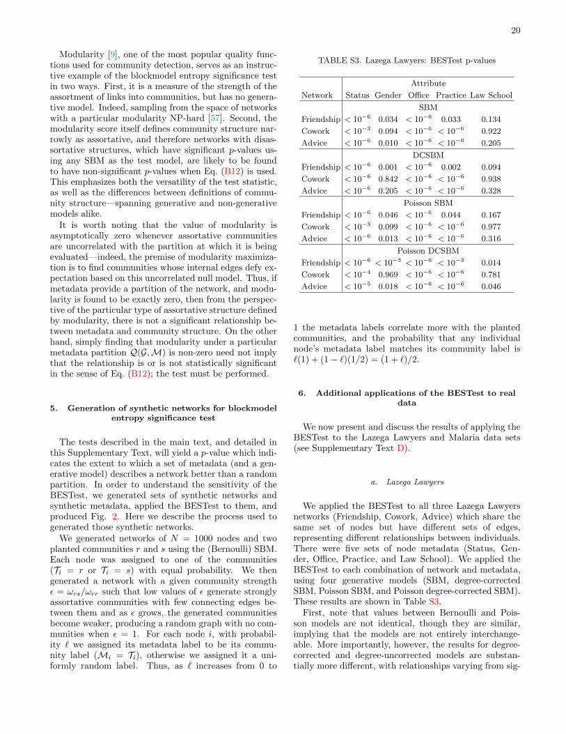
20

Modularity [9], one of the most popular quality func-tions used for community detection, serves as an instruc-tive example of the blockmodel entropy significance testin two ways. First, it is a measure of the strength of theassortment of links into communities, but has no genera-tive model. Indeed, sampling from the space of networkswith a particular modularity NP-hard [57]. Second, themodularity score itself defines community structure nar-rowly as assortative, and therefore networks with disas-sortative structures, which have significant p-values us-ing any SBM as the test model, are likely to be foundto have non-significant p-values when Eq. (B12) is used.This emphasizes both the versatility of the test statistic,as well as the differences between definitions of commu-nity structure—spanning generative and non-generativemodels alike.

It is worth noting that the value of modularity isasymptotically zero whenever assortative communitiesare uncorrelated with the partition at which it is beingevaluated—indeed, the premise of modularity maximiza-tion is to find communities whose internal edges defy ex-pectation based on this uncorrelated null model. Thus, ifmetadata provide a partition of the network, and modu-larity is found to be exactly zero, then from the perspec-tive of the particular type of assortative structure definedby modularity, there is not a significant relationship be-tween metadata and community structure. On the otherhand, simply finding that modularity under a particularmetadata partition Q(G,M) is non-zero need not implythat the relationship is or is not statistically significantin the sense of Eq. (B12); the test must be performed.

5. Generation of synthetic networks for blockmodelentropy significance test

The tests described in the main text, and detailed inthis Supplementary Text, will yield a p-value which indi-cates the extent to which a set of metadata (and a gen-erative model) describes a network better than a randompartition. In order to understand the sensitivity of theBESTest, we generated sets of synthetic networks andsynthetic metadata, applied the BESTest to them, andproduced Fig. 2. Here we describe the process used togenerated those synthetic networks.

We generated networks of N = 1000 nodes and twoplanted communities r and s using the (Bernoulli) SBM.Each node was assigned to one of the communities(Ti = r or Ti = s) with equal probability. We thengenerated a network with a given community strengthε = ωrs/ωrr such that low values of ε generate stronglyassortative communities with few connecting edges be-tween them and as ε grows, the generated communitiesbecome weaker, producing a random graph with no com-munities when ε = 1. For each node i, with probabil-ity ` we assigned its metadata label to be its commu-nity label (Mi = Ti), otherwise we assigned it a uni-formly random label. Thus, as ` increases from 0 to

TABLE S3. Lazega Lawyers: BESTest p-values

Attribute

Network Status Gender Office Practice Law School

SBM

Friendship < 10−6 0.034 < 10−6 0.033 0.134

Cowork < 10−3 0.094 < 10−6 < 10−6 0.922

Advice < 10−6 0.010 < 10−6 < 10−6 0.205

DCSBM

Friendship < 10−6 0.001 < 10−6 0.002 0.094

Cowork < 10−6 0.842 < 10−6 < 10−6 0.938

Advice < 10−6 0.205 < 10−6 < 10−6 0.328

Poisson SBM

Friendship < 10−6 0.046 < 10−6 0.044 0.167

Cowork < 10−3 0.099 < 10−6 < 10−6 0.977

Advice < 10−6 0.013 < 10−6 < 10−6 0.316

Poisson DCSBM

Friendship < 10−6 < 10−3 < 10−6 < 10−3 0.014

Cowork < 10−4 0.969 < 10−6 < 10−6 0.781

Advice < 10−5 0.018 < 10−6 < 10−6 0.046

1 the metadata labels correlate more with the plantedcommunities, and the probability that any individualnode’s metadata label matches its community label is`(1) + (1− `)(1/2) = (1 + `)/2.

6. Additional applications of the BESTest to realdata

We now present and discuss the results of applying theBESTest to the Lazega Lawyers and Malaria data sets(see Supplementary Text D).

a. Lazega Lawyers

We applied the BESTest to all three Lazega Lawyersnetworks (Friendship, Cowork, Advice) which share thesame set of nodes but have different sets of edges,representing different relationships between individuals.There were five sets of node metadata (Status, Gen-der, Office, Practice, and Law School). We applied theBESTest to each combination of network and metadata,using four generative models (SBM, degree-correctedSBM, Poisson SBM, and Poisson degree-corrected SBM).These results are shown in Table S3.

First, note that values between Bernoulli and Pois-son models are not identical, though they are similar,implying that the models are not entirely interchange-able. More importantly, however, the results for degree-corrected and degree-uncorrected models are substan-tially more different, with relationships varying from sig-

21

TABLE S4. Malaria: BESTest p-values for parasite originmetadata

Model

Network SBM DCSBM Poi. SBM Poi. DCSBM

Malaria 1 0.566 0.096 0.606 0.086

Malaria 2 0.064 0.148 0.066 0.143

Malaria 3 0.536 0.389 0.532 0.501

Malaria 4 0.588 0.617 0.604 0.644

Malaria 5 0.382 0.077 0.369 0.087

Malaria 6 0.275 0.923 0.293 0.751

Malaria 7 0.020 0.388 0.019 0.501

Malaria 8 0.464 0.176 0.468 0.172

Malaria 9 0.115 0.067 0.108 0.200

nificant under one model to insignificant under another.This highlights the fact that metadata can explain pat-terns of group structure in a network only through thelens of a particular network generative model; a change inthe model may impact the metadata’s ability to explainpatterns in network community structure.

Second, note that under all models, for each networkthere exist multiple sets of metadata that are significant.Similarly, there exist multiple networks for which anyindividual set of metadata is significant. This fundamen-tally undermines the notion that one should expect asingle set of metadata to function as ground truth, giventhat multiple sets of metadata explain multiple networks.

b. Malaria

We applied the BESTest to nine layers of a network ofmalaria parasite genes (Malaria 1-9) using four generativemodels (SBM, degree-corrected SBM, Poisson SBM, andPoisson degree-corrected SBM). Three sets of metadataexist for these networks, (parasite origin, CP group, andUPS), described in detail in Supplementary Text D.

The parasite origin results are shown in Table S4, andnone of the p-values listed is significant. This result in-dicates that when the nodes of each layer are dividedinto groups based on parasite origin, the entropy of theresulting model is no better than assigning the nodes togroups at random. This implies, in turn, that the malariaparasite antigen genes do not group by the parasite fromwhich they came, confirming previous observations [41].However, as shown in Fig. 2 the BESTest is sensitive toeven small levels of explanatory power provided by meta-data, indicating that parasite origin has truly no bearingon the community structure of malaria parasite antigengenes, for all four generative models tested.

On the other hand, it is known that the genes repre-sented by the nodes of the malaria parasite networks arecorrelated with CP group and UPS metadata. As shownin Tables S5 and S6 the BESTest indeed finds that this is

the case, with a handful of exceptions, again confirmingprevious results that used less sophisticated techniques[41].

TABLE S5. Malaria: BESTest p-values for CP group meta-data

Model

Network SBM DCSBM Poi. SBM Poi. DCSBM

Malaria 1 < 10−5 < 10−5 < 10−5 < 10−5

Malaria 2 < 10−5 < 10−5 < 10−5 < 10−5

Malaria 3 < 10−5 < 10−5 < 10−5 < 10−5

Malaria 4 < 10−5 < 10−5 < 10−5 < 10−5

Malaria 5 < 10−5 < 10−5 < 10−5 < 10−5

Malaria 6 < 10−5 < 10−5 < 10−5 < 10−5

Malaria 7 < 10−5 < 10−5 < 10−5 < 10−5

Malaria 8 < 10−5 < 10−5 < 10−5 < 10−5

Malaria 9 < 10−5 < 10−5 < 10−5 < 10−5

TABLE S6. Malaria: BESTest p-values for UPS metadata

Model

Network SBM DCSBM Poi. SBM Poi. DCSBM

Malaria 1 < 10−5 < 10−5 < 10−5 < 10−5

Malaria 2 < 10−5 < 10−5 < 10−5 < 10−5

Malaria 3 < 10−5 < 10−5 < 10−5 < 10−5

Malaria 4 < 10−5 < 10−5 < 10−5 < 10−5

Malaria 5 < 10−5 < 10−5 < 10−5 < 10−5

Malaria 6 < 10−5 < 10−5 < 10−5 < 10−5

Malaria 7 < 10−5 < 10−5 < 10−5 < 10−5

Malaria 8 < 10−5 < 10−5 < 10−5 < 10−5

Malaria 9 < 10−5 < 10−5 < 10−5 < 10−5

Morpheus: The Matrix is a system, Neo. That systemis our enemy. But when you’re inside, you look around,what do you see? . . . The very minds of the people weare trying to save. But until we do, these people are stilla part of that system and that makes them our enemy.You have to understand, most of these people are notready to be unplugged. And many of them are so inured,so hopelessly dependent on the system, that they will fightto protect it. [61]

22

Appendix C: No optimal community detectionalgorithm

Spoon boy: Do not try and bend the spoon—that’s im-possible. Instead, only try to realize the truth.Neo: What truth?Spoon boy: There is no spoon.Neo: There is no spoon?Spoon boy: Then you will see that it is not the spoonthat bends, it is only yourself. [61]

In the main text we argue that that the goal of re-covering ground truth communities is ill posed becauseit lacks a unique solution and we also claim a “No FreeLunch” theorem for community detection. In this Sup-plementary Text, we describe and expound those claimsusing technical arguments.

For convenience, we provide a reference table of nota-tion used in derivations in this Supplementary Text.

TABLE S7. Notation used in this Supplementary Text

Variable Definition

G a network, G = (V,E)

N the number of nodes |V |T ground truth (planted) partition

C detected communities partition

g generative model, maps a partition to a network. G = g(T )

f comm. detection method, maps G to a partition C = f(G)

`(·, ·) an error or loss function, returns a scalar

X the space of possible inputs, i.e., all possible graphs GY the space of possible outputs, i.e., all possible partitions

γ the true relationship between X and Y

h the hypothesis about the relationship between X and Y

σX probability density over X

Λ(`) total loss across all possible inputs for loss function `

u, v two partitions of N objects

Ω the set of all possible partitions of N objects.

BN the Nth Bell number, the number of possible ways

that N objects can be partitioned. B = |Ω|

1. Ground-truth community detection is anill-posed inverse problem

A problem that is well posed satisfies three proper-ties: (i) a solution exists, (ii) the solution is unique, and(iii) the solution’s behavior changes continuously withthe problem’s initial conditions. The classic example ofan ill-posed problem is the inverse heat equation, whichviolates condition (iii) because its solution (the distri-bution of temperature in the past) is highly sensitiveto changes in the distribution of temperatures at thepresent. The problem of reproducing ground truth com-munities T from a network G by formulating the correctcommunity detection algorithm f∗ is ill posed because

it fails condition (ii), i.e., community detection has nounique solution.

Definition: The ground truth communitydetection problem: given a fixed networkG in which there has been hidden someground truth partition T , find the truecommunities that were planted in, embed-ded in, or used to generate the network. Inother words, given G, find the T such thatG = g(T ).

We now argue that the ground truth community de-tection problem is ill posed because its solution is notunique. The intuition behind this argument is that anynetwork G could have been created using many differ-ent planted partitions via different generative processes.Therefore, searching for the ground truth partition with-out knowing the exact generative mechanism is an im-possible task; there is no ground truth.

Theorem 1: For a fixed network G, the so-lution to the ground truth community de-tection problem is not unique.

Proof: We first show that the graph G can be producedby using two different planted partitions, T1 and T2 withT1 6= T2. Let T1 be the trivial 1-partition in which allvertices are in the same group, and let g1 be the gener-ative model of Erdos-Renyi random graphs with proba-bility p ∈ (0, 1). Then the model and partition g1(T1)create G with non-zero probability. Let T2 be the triv-ial N -partition in which each vertex is in its own group,and let g2 be a generative model that specifies the ex-act number of edges between all groups, such that g2(T2)produces G with probability one. We therefore have twopartitions T1 6= T2 and both g1(T1) and g2(T2) can createG. Since two different planted partitions may be respon-sible for G, both are potential solutions of the communitydetection problem. Therefore, the solution to the com-munity detection problem is not unique for the networkG. To complete the proof, note that the 1-partition andN -partition argument above applies equally well to anynetwork G.

The theorem above relies on two trivial partitions, the1-partition and the N -partition in its proof, but otherexamples exist as well: consider the generative modelgG∗ which maps any partition that it is given to somefixed network G∗, essentially ignoring the informationprovided by the partition [similar to case (i) in the maintext]. These models, while sufficient for the proof, arenot particularly interesting for practictioners, yet non-trivial models and partitions also exist for any network.For instance, the Karate Club network may have plau-sibly been produced by the SBM with a core-peripherypartition or by the degree-corrected SBM with a socialfaction partition [20].

Belief in ground truth T necessitates a belief in a spe-cific generative mechanism g which together producedthe network G. For real-world networks, which may arise

23

through more complex processes than those describedhere, we do not know the generative mechanism. Theo-rem 1 means that, in these cases, it is impossible to re-cover the true partition because any partition may plau-sibly have been used to generate the network. There-fore the ground truth community detection problem isill-posed for any network for which the generative pro-cess is unknown because there is no unique solution. Putdifferently, it is impossible to uniquely solve an inverseproblem when the function to be inverted is not a bijec-tion.

2. No Free Lunch for community detection

The “no free lunch” (NFL) theorem [32] for machinelearning states that for supervised learning problems, theexpected misclassification rate, summed over all possibledata sets, is independent of the algorithm used. In otherwords, averaged over all problems, every algorithm hasthe same performance. Therefore, if algorithm f1 out-performs algorithm f2 for one set of problems, then thereexists some other set of problems for which algorithm f2

outperforms algorithm f1. In other words, it is impossi-ble to get overall better performance without some cost;there is no free lunch.

The NFL theorem holds for community detection, andclustering problems in general. Demonstrating this re-quires that we first translate the community detectionproblem into the language and notation of the ExtendedBayesian Framework (EBF) used in the NFL theoremsfor supervised learning. Then, under an appropriatechoice of error (or “loss”) function `, the performanceof any community detection method f , summed over allproblems g, T , is identical∑

g,T`(T , f (g(T ))

)= Λ(`) ∀f , (C1)

where Λ(`) depends on the particular error function ` butis otherwise a constant, representing the total error.

In the following, we map community detection nota-tion to EBF notation, provide a guiding example, andthen resolve a subtle issue related to the loss function`. We then discuss the implications of this result for fu-ture studies of community detection. The proofs of theNFL theorems are not recapitulated here, but are fullydetailed in Ref. [32] and discussed extensively elsewhere.

a. Community detection in the Extended BayesianFramework

The Extended Bayesian Framework (EBF) is aframework—a set of variables, definitions, andassumptions—for supervised learning that providesa clear and precise description of the problem. It isimportant in both the proof and implications of the

NFL theorem, and was formalized at length in Ref. [32].In what follows, random variables will be denotedby capital letters, e.g. X, while instances of randomvariables will be denoted by the corresponding lowercaseletters, e.g. x. In the EBF, we suppose that there existsan input space X, an output space Y , and that eachof these has a countable (but possibly infinite) numberof elements, |X| = n and |Y | = r. The fundamentalrelationship to be learned is how X and Y are related,and to that end, let γ be the true or target relationshipbetween X and Y , i.e., γ is the conditional distributionof Y , given X. The points in the space X need not bedistributed uniformly either, so we also specify σ, theprobability density function of points x in the inputspace X, i.e., P (x|σ) = σX . In the nomenclature ofcommunity detection, the input x ∈ X is simply theobserved graph G, and the output y ∈ Y is the truepartition into communities T for the nodes described byx. To solve a community detection problem, we hopeto predict the true communities y from the input graphx; a community detection method will be successfulwhen its hypothesized relationship h is an accuraterepresentation of the true relationship γ between X andY .

In supervised learning, for which the NFL theoremswere originally proved, we aim to learn the relation-ship between X and Y from a training set d whichconsists of m ordered pairs of samples from X and Y ,dX(i), dY (i)mi=1. In response to the training data, thelearning algorithm produces a hypothesis h in the formof an x-conditioned probability distribution over valuesy. The way in which the learning algorithm producesa hypothesis from training sets is described by P (h|d),the distribution over hypotheses conditioned on the ob-served data. Note that the algorithm learns from the dataalone and is independent of γ, i.e., P (h|d, f) = P (h|d).If the algorithm performs well the hypothesis h will havehigh correspondence with the true relationship γ. There-fore, in supervised learning, algorithms are evaluated bytheir ability to make sufficient use of a limited train-ing set to provide good predictions of y given x not inthe training set. On the other hand, in unsupervisedlearning—a category which includes clustering and com-munity detection—the training set d is empty (m = 0),so the prediction h is based solely on the prior beliefs en-coded in the model P (h). We note that in the NFL the-orems for supervised learning, the independence of train-ing data d from γ and σ is important to establish, butfor unsupervised tasks, the set d is empty so it is triviallyindependent of γ and σ.

To better understand the EBF for community detec-tion, an example is helpful. Consider the problem offinding two planted communities in a network G. Thetrue relationship γ between the network and its parti-tion is hidden. Given only G—which is a point in thespace of graphs X—fitting the parameters of an SBM,maximizing modularity, or using another method of ourchoice, produces a hypothesis h, which is a prediction

24

about which nodes belong to which groups. If these com-munities are found correctly by the algorithm, then h willbe highly correlated with the true communities mappedby γ. (This is equally true for both hard partitions,where each node belongs to only one group, and soft par-titions, where each node may be distributed over multiplegroups.) In other words, h estimates γ based on a pointin X called G. Because the estimate h is based only onG and the assumptions of the algorithm P (h), it repro-duces γ with possibly limited accuracy, and therefore itscommunity assignments may or may not be highly cor-related with the true assignments T ∈ Y . Increasing thesize of the input data set may help with accuracy as well:by generating a larger graph using the same generativemodel, G supplies a different point in X providing moreinformation to the community detection method. Thismay allow the estimate h to produce better predictionsof γ, thereby producing a more accurate partitioning ofnodes into their true communities, but only if the modelP (h) is sufficiently aligned to reality P (γ).

All learning algorithms make some prior assumptions,in the form of P (h), about the possible relationships be-tween inputs and outputs. For unsupervised methodssuch as community detection, there is a much greaterimportance associated with these assumptions becausethey do not have access to training data. For instance, asupervised algorithm could supposedly start from a uni-formly ignorant prior P (h) and rely on having a suf-ficiently large training set that P (h|d) is informative.When there is no training data it is necessary that P (h)is informative of the possible input-output relationship.Thus, community detection algorithms encode beliefs ordefinitions of community structure, and these beliefs con-stitute a prior over the kinds of problems that we expectto see. Some methods, for example, search only for as-sortative [9, 37] or disassortative [38] community struc-tures, while other are more flexible and can find mixturesof assortative, disassortative, and core-periphery struc-tures [15, 16, 20, 39] and allow for nodes to belong tomultiple communities [36, 37].

b. Loss functions and a priori superiority

So far, we have discussed the phrasing of communitydetection in the language of EBF but have not describedthe way in which error (also called loss or cost) is mea-sured. The error function quantifies the accuracy of pre-dictions, and the EBF introduces a random variable Cwhich represents the error associated with a particularγ and h, i.e., the error associated with using a par-ticular algorithm for a particular problem. Conceptu-ally, this is what the community detection literature at-tempts to estimate when algorithms are compared basedon their ability to recover planted communities in syn-thetic data. More formally, C is measured by the distri-bution P (c|h, γ, d), which incorporates the relationshipsbetween the test set and the generating process, as well as

1 2 3 4 5FIG. S6. The five distinct ways to partition three nodes. Nor-malized mutual information and adjusted mutual informationbetween each pair of partitions are presented in Tables S8 andS9, respectively.

the way in which the hypothesis is related to the trainingdata. Therefore, the quantity of interest to those devel-oping algorithms is the expected error, E(C|h, γ, d). Forexample, in the context of supervised learning, choosingthe loss function ` to be the average misclassification rateis common. For the purposes of community detection,misclassification rate is not of interest for a pedantic butimportant reason: for community detection and other re-lated unsupervised tasks such as clustering, permutationsof the group labels are inconsequential because the parti-tion is the desired outcome; labeling two groups a and bis equivalent to labeling them b and a. As a result, manyof the loss functions typically used to compare partitionshave a “geometric” structure that implies an a priori su-periority of some algorithms, which would appear to con-tradict the NFL theorem. We now discuss one such lossfunction frequently used to evaluate community detec-tion algorithms, the normalized mutual information, andthe structure that it imposes on the space of partitions.

Normalized mutual information is an information-theoretic measurement of similarity between two parti-tions that treats both partitions as statistical objects.For a partition u of N objects into Ku groups, the prob-ability that an object chosen uniformly at random fallsinto group ui is pi = |ui|/N , i = 1 . . .Ku. The entropyassociate with a partition u is then the entropy of itscorresponding distribution p,

H(u) = −Ku∑i=1

pi log (pi) .

When comparing two partitions u and v of the same setof objects, each object belongs to some group ui in thefirst partitions and some other group vj , j = 1 . . .Kv inthe second partition, with the corresponding probabilitypij . The mutual information between the two partitions

25

is therefore

I(u, v) =

Ku∑i=1

Kv∑j=1

pij log

(pijpipj

),

which can be normalized to define normalized mutualinformation as

NMI(u, v) =I(u, v)√H(u)H(v)

. (C2)

Other normalizing factors in the denominator are possi-ble, including 1

2 [H(u)+H(v)] and maxH(u), H(v); see[58]. NMI maps partitions to the unit interval, with 0indicating that two partitions are uncorrelated and 1 in-dicating that they are identical (even if the groups labelsdiffer).

To understand how an error function imposes a ge-ometric structure, consider a simple problem (unre-lated to community detection) of predicting, based onsome inputs X, a point in the unit circle in Y =y∣∣ ‖y‖ ≤ 1, y ∈ R2

. If all points in Y are equally

likely, then an algorithm that guesses the center of thecircle h = 0 will outperform an algorithm that guesses apoint on the boundary h ∈ ∂Y , simply due to the factthat the center of the circle is, on average, closer to theother points of the circle than any boundary point. Nor-malized mutual information imposes a geometric struc-ture on the space of partitions in a similar way.

Consider a loss function based on normalized mutualinformation (NMI) and imagine a community detectionalgorithm that entirely ignores the network and simplyreturns a fixed partition of the vertices. As in the ex-ample above, NMI provides a geometrical structure onthe space of partitions, an algorithm that always returnsa partition toward the middle of the space of partitionswill outperform an algorithm that always returns a par-tition on the boundary of that space. To demonstratethis point, Fig. S6 shows all five possible partitions ofthree vertices, and Table S8 shows their NMI for all pair-wise comparisons. Averaged over all possible correct an-swers, an algorithm that consistently predicts partition 5will outperform all others, and an algorithm that consis-tently predicts partition 1 will underperform all others.However, this structure is a known issue of NMI, and soother error functions and corrections have been proposedsuch as the adjusted mutual information (AMI), whichaccounts for the geometry of the space [58]. Table S9shows the AMI for the same set of partitions, and theexpected AMI is zero except for the partition that con-tains only a single group and the partition of each nodeinto separate groups. In the case of these partitions, the1-partition and the N -partition, the expected AMI is thereciprocal of the Bell number BN—the Bell number is thetotal number of distinct ways that N objects can be par-titioned, and it grows superexponentially with N—so asthe number of vertices N increases, so AMI approaches 0superexponentially; for even small networks, 1/BN ≈ 0.In this way, AMI provides a “geometry-free” space in

TABLE S8. Normalized mutual information for partitions inFig. S6

Partition 2

Partition 1 1 2 3 4 5

1 1 0 0 0 0

2 0 1 0.27 0.27 0.76

3 0 0.27 1 0.27 0.76

4 0 0.27 0.27 1 0.76

5 0 0.76 0.76 0.76 1

E[NMI] 0.20 0.46 0.46 0.46 0.66

TABLE S9. Adjusted mutual information for partitions inFig. S6

Partition 2

Partition 1 1 2 3 4 5

1 1 0 0 0 0

2 0 1 -0.5 -0.5 0

3 0 -0.5 1 -0.5 0

4 0 -0.5 -0.5 1 0

5 0 0 0 0 1

E[AMI] 0.20 0 0 0 0.20

which no one partition is a priori closer to all others.This key property of AMI, called homogeneity, is provedin a Lemma in the next section.

c. Lemma and theorems

We now prove a lemma about adjusted mutual infor-mation, and then formally state the NFL theorem forsupervised learning and prove the no free lunch theoremfor community detection.

Lemma 1: Adjusted mutual information(AMI) is a homogenous loss function overthe interior of the space of partitions of Nobjects. Including the boundary partitions,i.e., the 1-partition and the N -partition,AMI is homogenous within B−1

N .

Proof: Showing that AMI is a homogenous loss functionrequires that we show

L(u) =∑v∈Ω

AMI(u, v) (C3)

is independent of u, where Ω is the space of all partitionsof N objects. Stated plainly, if L(u) is independent ofu, it means that the total AMI between partition u andall possible partitions will be the same, no matter which

26

partition u is chosen. The definition of AMI is:

AMI(u, v) =I(u, v)− E[I(u, v)]√H(u)H(v)− E[I(u, v)]

where I is mutual information and H is entropy [58]. TheAMI takes on a value of 1 when two partitions are identi-cal and a value of 0 when they are only correlated to theextent that one would expect by chance. In particular,the expectation E is taken over all possible pairs of par-titions u′ and v′ such that every u′ has the same numberof groups and the same number of objects belonging toeach group as does u, and likewise for v′ and v. In thisway, the expectation E is taken over all pairs of divisionsthat preserve the group sizes of the two partitions beingcompared. For convenience of notation, let φ be a sub-set of all partitions Ω such that every partition v ∈ φhas the same number of groups and same number of ob-jects in each group. The set of all partitions Ω may besubdivided into non-overlapping subsets φi, such that∪iφi = Ω and φi ∩ φj = ∅ for any i 6= j. (For example,in Fig. S6, partition 1 belongs to φ1, partitions 2, 3, and4 belong to φ2, and partition 5 belongs to φ3.) Let theparticular subset φi to which a partition u belongs bedenoted by φ(u).

Prior to proceeding, we note that there are two specialboundary partitions, the 1-partition in which all objectsare in a single group and the N -partition in which eachobject is in its own group. These will be denoted by 1 andN respectively. Note that 1 = φ(1) so that |φ(1)| = 1,and that φ(N) is equivalent to the set of all possiblerelabelings of the N objects, so that |φ(N)| = N ! .Because there is only one element of φ(1), it is nec-essarily true that I(1, 1) = E[I(1, 1)] = H(1). Thus,for this special case, the numerator and denominator ofAMI are identical, and AMI(1, 1) = 1. Similarly, be-cause the set φ(N) contains every possible permutationof the labels of the objects, yet all partitions are identical,I(N , N) = E[I(N , N)] = H(N), and so AMI(N , N) = 1.

In order to prove Eq. (C3), we will show that L(u) =0 for all u except 1 and N by demonstrating that thenumerator of the definition of AMI is 0, specifically,∑

v∈Ω

[I(u, v)− E[I(u, v)]] = 0 ∀ u 6= 1 or N . (C4)

In fact, we will show that Eq. (C4) holds by breaking theentire sum over all partitions Ω into sums over each ofits disjoint subsets φi, and proving that∑

v′∈φ(v)

[I(u, v′)− E[I(u, v′)]] = 0

∀ u and ∀ v except u = v = 1 or u = v = N . (C5)

In other words, we will show that the numerator of thedefinition of AMI is equal to zero when summed over anysubset φ(v) for any fixed partition u, except the bound-ary cases that both u and v are equal to 1 or both areequal to N . We first examine the expectation term in

Eq. (C5). Recall that the expectation is taken over allpairs of members of the subsets φ(u) and φ(v), respec-tively,

E[I(u, v)] =1

|φ(u)||φ(v)|∑

u′∈φ(u)

∑v′∈φ(v)

I(u′, v′) . (C6)

In fact, because the sums above are taken over the sub-sets φ(u) and φ(v) that contain u and v, the expectedmutual information is equal to a constant ζ for any pairof partitions drawn from φ(u) and φ(v),

E[I(u, v)] = ζ ∀ u ∈ φ(u) and ∀ v ∈ φ(v) . (C7)

Note then that we may rewrite the sum over expectationsin Eq. (C5) as

∑v′∈φ(v)E[I(u, v′)] = |φ(v)| ζ. Therefore,

it remains to be shown that the sum over mutual infor-mations in Eq. (C5) is also equal to |φ(v)| ζ,∑

v′∈φ(v)

I(u, v′) = |φ(v)| ζ . (C8)

To see that this is true, despite the fact that u is fixed(and not averaged over all u′ ∈ φ(u) as in E[I(u, v)]),note that Eq. (C8) nevertheless sums over every v′ ∈ φ(v)which is the set of every randomization of the partitionv, provided group sizes are held constant. Because thisincludes all relabelings (or reindexings) of the N objectsbeing partitioned, it must be true that,∑v′∈φ(v)

I(u1, v′) =

∑v′∈φ(v)

I(u2, v′) whenever u1 ∈ φ(u2) .

(C9)In other words, the sum of mutual information between afixed partition u1 and all members of a subset φ(v) mustbe equal to the sum of mutual information between adifferent fixed partition u2 and the same subset φ(v), butonly if u1 and u2 both belong to the same subset as eachother. Therefore, Eq. (C8) is true, meaning that the sumover the two terms in Eq. (C5) is zero, independent of u.This first implies that the AMI between any boundarypartition and any interior partition is 0, AMI(u, 1) = 0for any u 6= 1 and AMI(u, N) = 0 for any u 6= N . This,in turn, implies Eq. (C4) is true. This completes theproof of the first statement, that Eq. (C3) is true, andin particular, L(u) = 0, for any u 6= 1, N and AMI ishomogeneous over all non-boundary partitions.

In the special cases of u = v = 1 and u = v = N ,note that we have already shown that AMI(1, 1) = 1,AMI(N , N) = 1, and AMI(u, 1) = 0 for any u 6= 1 andAMI(u, N) = 0 for any u 6= N . Therefore,

L(1) =∑v∈Ω

AMI(1, v) = B−1N ,

L(N) =∑v∈Ω

AMI(N , v) = B−1N , (C10)

completing the proof of the second statement: includ-ing the boundary points, AMI is homogenous within anadditive constant B−1

N .

27

Theorem 2 (Wolpert 1996): For homo-geneous loss `, the uniform average over allγ of P (c|γ, d) equals Λ(c)/r.

Proof: See Ref. [32].

Theorem 3 (No free lunch for com-munity detection): For the communitydetection problem with a loss function ofadjusted mutual information, the uniformaverage over all γ of P (c|γ) equals Λ(c)/r.

Proof: Lemma 1 proves that adjusted mutual informationis homogeneous and applying Theorem 2 with d = ∅completes the proof.

d. Implications

No free lunch for community detection means that,uniformly averaged over all community detection prob-lems, and evaluated by AMI, all algorithms have equiv-alent performance. Phrased more usefully, it means thatany subset of problems for which an algorithm outper-forms others is balanced by another subset for which thealgorithm underperforms others. Thus, there is no singlecommunity detection algorithm that is best overall.

On the other hand, if the set of problems of interest isa non-uniform subset of all problems, then one algorithmmay outperform another on this subset. In other words,the bias of an algorithm to solving a particular type ofcommunity detection problem may be its strength, ac-cepting the fact that such an advantage must be balancedby disadvantages elsewhere. For instance, algorithms likethe unconstrained SBM (which can find both assortativeand disassortative communities and mixtures and gra-dations thereof) are not universally superior to versionsof the SBM constrained to find only assortative or dis-assortative communities [38]—if the particular subset ofproblems is believed to contain only disassortative com-munities, then the unconstrained SBM will not performas well as a constrained one. In other words, no freelunch for community detection means that matching theassumptions in the model to the underlying generativeprocess can lead to better, more accurate results, butonly in the cases when the beliefs about the underlyinggenerative process are accurate; in the other cases, thesame model assumptions that improved performance onsome problems will diminish it for others. To some extentwe expect the distribution of problems to be non-uniformin general. Out of all the possible ways of constructing agraph there may be some types of graph we are less likelyto observe. For each graph we can also expect that of allthe possible partitions, many will correspond to randomassignments of nodes that are not useful in any appli-cation. Put differently, there may be some problems wedo not wish to solve—but, unless we know which prob-lems they are, it offers us little or no benefit in practice.We note that relatively little is known about which al-gorithms perform better than others within particular

domains or on particular classes of networks. A valuableline of future research on community detection will bedeveloping such an understanding [50, 51].

Cypher: You know, I know this steak doesn’t exist. Iknow that when I put it in my mouth, the Matrix is tellingmy brain that it is juicy and delicious. After nine years,you know what I realize? . . . Ignorance is bliss. [61]

28

Appendix D: Datasets and additional methodology

Neo:Whoa. [61]

1. Lazega Lawyers networks

The Lazega Lawyers network is a multilayer networkconsisting of 71 attorneys of a law firm with three differ-ent sets of links, corresponding to friendships, exchangeof professional advice, and shared cases [42]. The origi-nal study also collected five sets of categorical node meta-data, corresponding to status (partner or associate), gen-der, office location, type of practice (corporate or liti-gation), and law school (Harvard, Yale, UConn, other).The relationships and dynamics within the law firm werestudied extensively in the initial publication of these datasets, but they were not primarily analyzed as complexnetworks.

2. Malaria var gene networks

The Malaria data set consists of 307 var gene sequencesfrom the malaria parasite P. falciparum [41]. Each vargene encodes a protein that the parasite uses to evadethe human immune system, and therefore this family ofgenes is under intense evolutionary pressures from thehuman host. The original study focused on uncoveringthe functional and evolutionary constraints on var geneevolution by identifying community structure in var genenetworks.

These sequences were independently analyzed at 9loci (locations within the genes), producing 9 differentgenetic-substring-sharing networks with the same nodeset. In other words, there are 9 layers in this multi-layer network. Each parasite genome contains around60 var genes, and the 307 genes in this data set repre-sent seven parasite genomes. The original study includedthree sets of categorical node metadata, correspondingto the upstream promoter sequence classification (UPS,K = 3), CysPoLV groups (CP K = 6), and the parasitegenome from which sequence was generated (parasite ori-gin K = 7).

3. Karate Club network

The Zachary Karate Club represents the observed so-cial interactions of 34 members of a karate club [14]. Atthe time of study, the club fell into a political disputeand split into two factions, which are treated as meta-data. The Karate Club has been analyzed exhaustivelyin studies of community detection, and its faction meta-data have often been used as ground truth for community

detection, due to the network’s small size and easily in-terpretable social narrative.

4. Generation of log-likelihood surface plots

The log-likelihood surface plots in Figs. 1, 3, 4, S1,S2, and S3 illustrate the changes in log likelihood as thepartition of network nodes is varied. In the figures, weshow surfaces that appear to be continuous over that twodimensional space, in spite of the fact that the true spaceof partitions is high dimensional and discretized, and sohere we explain the methods used to produce visuallymeaningful plots.

Plots were generated in three steps: partition sam-pling, data projection and surface interpolation. Formost networks it is infeasible to calculate the log like-lihood of all possible partitions, so we instead sampled asubset of partitions. We began with the set of partitionsalong the path of the neoSBM (e.g., Fig. 3) and sampledpartitions around the local neighborhood of this initialset. Specifically, we did so by selecting two partitionsuniformly at random from the initial set and created eachnew partition by assigning q nodes (chosen randomly anduniformly) to the group assignment of the first partitionand the remaining N − q nodes to that of the secondpartition.

Next, we projected the KN -dimensional partition datadown to two dimensions using Multi-dimensional Scal-ing (MDS) [59] and variation of information [60] as asimilarity measure. The outcome of this projection wasa two-dimensional representation of the partition spacethat preserves the variation of information between par-titions.

Finally, we used MATLAB’s scatteredInterpolant func-tion with natural interpolation to fit an interpolated sur-face to the data, which we evaluated over a grid of do-main points and smoothed using a Gaussian kernel toimprove legibility. The processes of embedding, interpo-lating, and smoothing are not particularly sensitive tochanges in parameters or grid resolutions.

In the special case of Fig. 4, we also plotted the par-titions of the neoSBM in addition to the interpolatedlog-likelihood surface to illustrate the neoSBM’s path inthe broader context of the surface. There were no modifi-cations or smoothing of the points of the neoSBM’s pathbeyond the embedding process described above.

Neo: I know you’re out there. I can feel you now. Iknow that you’re afraid . . . you’re afraid of us. You’reafraid of change. I don’t know the future. I didn’t comehere to tell you how this is going to end. I came hereto tell you how it’s going to begin. I’m going to hang upthis phone, and then I’m going to show these people whatyou don’t want them to see. I’m going to show them aworld without you. A world without rules and controls,without borders or boundaries. A world where anythingis possible. Where we go from there is a choice I leave toyou. [61]