J Econ Growth (2010) 15:127–153DOI 10.1007/s10887-010-9051-0

The Green Solow model

William A. Brock · M. Scott Taylor

Published online: 16 May 2010© Springer Science+Business Media, LLC 2010

Abstract We argue that a key empirical finding in environmental economics—the Envi-ronmental Kuznets Curve (EKC)—and the core model of modern macroeconomics—theSolow model—are intimately related. Once we amend the Solow model to incorporate tech-nological progress in abatement, the EKC is a necessary by product of convergence to asustainable growth path. We explain why current methods for estimating an EKC are likelyto fail; provide an alternative empirical method directly tied to our theory; and estimate ourmodel on carbon emissions from 173 countries over the 1960–1998 period.

Keywords Environment · Environmental Kuznets Curve · Carbon emissions ·Solow model · Sustainability · Pollution

1 Introduction

The goal of this paper is to provide a cohesive theoretical explanation for three puzzlingfeatures of the pollution and income per capita data. To do so we introduce the reader toa very simple growth model closely related to the one-sector Solow model and show howthis amended model generates predictions closely in line with U.S. and European evidenceon emissions, emission intensities and pollution abatement costs. The model provides anexplanation for the sometimes confusing and fragile empirical results present in the growthand environment literature, while offering an alternative testing methodology tightly tied totheory. Importantly, it resolves several puzzles related to the Environmental Kuznets Curve

W. A. BrockDepartment of Economics, University of Wisconsin, Madison, WI, USA

M. S. Taylor (B)Department of Economics, Faculty of Social Science, University of Calgary, Calgary, AB, Canada

M. S. TaylorNational Bureau of Economic Research, Cambridge, MA, USA

123

128 J Econ Growth (2010) 15:127–153

which is an empirical finding linking rising per capita income levels with a first deterioratingand then improving environment.

While our work is related to recent attempts to explain the Environmental Kuznets Curve(thereafter EKC) it differs in several important ways. First, we attempt to fit more features ofthe data than just the relationship between pollution emissions and per capita income levels;specifically, we employ data on both pollution abatement costs and emission intensities toargue that key features of the data are largely inconsistent with existing theories. Second,we argue these data are well explained by a very simple variant of the Solow model wheretechnological progress in abatement and diminishing returns to capital play leading roles. Bydoing so we argue that the forces of diminishing returns and technological progress identifiedby Solow as fundamental to the growth process, may also be fundamental to the EKC find-ing. Third, to demonstrate the potential usefulness of our approach we derive an estimatingequation directly from theory and evaluate the model using carbon data from 173 countriesover the 1960–1998 pre-Kyoto period.

The EKC has captured the attention of policymakers, theorists and empirical researchersalike since its discovery in the early 1990s.1 The theory literature has from the start focusedon developing models that replicate the inverted U shaped relationship. Prominent explana-tions are threshold effects in abatement that delay the onset of policy, income driven policychanges that get stronger with income growth, structural change towards a service basedeconomy, and increasing returns to abatement that drive down costs of pollution control.2

While each of these explanations succeeds in predicting a EKC, they are typically lesssuccessful at matching other features of the income and pollution data. One key feature of thisdata concerns the timing of pollution reductions. Models of threshold effects predict no pol-lution policy at all over some initial period followed by a period of active regulation.3 Whenpolicy is inactive, emissions are produced in proportion to output. When policy becomesactive, the emissions to output ratio declines sharply and immediately aggregate emissionsfall. The available data on pollution emissions is however inconsistent with this strong tem-poral correlation. Emissions per unit output typically decline well before any reduction inaggregate emissions.

A second feature of the data that is difficult to reconcile with many theories is the timeseries of pollution abatement costs. Theories that rely on rising incomes driving down emis-sions via tighter pollution policy must square the very large fall in emissions with pollutionabatement costs that although rising, appear almost constant as a fraction of overall output.For example U.S. Sulfur Dioxide emissions peaked in 1973 at approximately 32 milliontons and fell almost in half to approximately 17 million tons in 2001. Correspondingly largechanges in emissions per unit output also occurred. But over much of this period, pollu-tion abatement costs as a fraction of GDP or manufacturing value-added, remained smalland, most importantly, without much of a positive trend. Theories that rely on tighteningenvironmental policy predict ever increasing costs of abatement, since emissions per unit ofoutput must fall faster than aggregate output to hold pollution in check. In a world withouttechnological progress in abatement, this requires larger and larger investments in pollutioncontrol.4

1 See Grossman and Krueger (1994) and Grossman and Krueger (1995) for example.2 For original contributions see Stokey (1998), Andreoni and Levinson (2001), and Lopez (1994). A reviewof these and other competing explanations appears in Chap. 2 of Copeland and Taylor (2003).3 This is for example the exact prediction of both Stokey (1998) and Brock and Taylor (2003).4 Stokey (1998), Aghion and Howitt (1998) and others adopt an abatement function relating emissions per unitfinal output, E/Y , to the share of productive factors used in abatement θ , as follows: E/Y = (1−θ)β , β > 0.

123

J Econ Growth (2010) 15:127–153 129

Theories relying on strong compositional shifts or increasing returns also havedifficulty matching these data. Empirical work has found a changing composition of out-put plays at most a bit part in the reductions we have observed (Selden et al. 1999; Bruvolland Medin 2003). And while increasing returns to abatement may be important in some indus-tries and for some processes, a large portion of emissions come from small diffuse sourcessuch as cars, houses and individual consumptive activity. In each of these cases, increasingreturns to abatement seems unlikely. Increasing returns also presents strong incentives formergers and natural monopoly and unless we bound the strength of increasing returns care-fully, increasing-returns-to-scale models predict negative pollution emissions at large levelsof output.5

To us, the pollution data and the related empirical work on the EKC present three puzzlesthat need to be resolved by any successful theory. The first puzzle is how do we square theongoing large reductions in emission intensities with the relatively static pollution abatementcosts? The second puzzle is the EKC: what is responsible for the humped-shape profile ofpollution levels when graphed against time or income per capita? The third puzzle comesfrom the empirical literature itself. It is now well known that empirical estimates from EKCstyle regressions can vary greatly with the sample used and estimation procedure. Do thesefragile cross-country empirical results imply that the EKC does not exist, or is the problemthe use of empirical methods that are subject to wide variance?

In this paper we show that the Green Solow model provides a very simple explanation forall three puzzles. In addition, the model also suggests an alternative empirical methodologytightly tied to theory. We demonstrate that a robust prediction of the Green Solow model isconvergence in emissions per capita across countries. This prediction holds when the pollu-tant in question follows an EKC pattern to eventually diminish, but importantly also holdsif growth is unsustainable and no EKC pattern emerges. This convergence prediction can beevaluated in a number of ways, and indeed there already exists a sizeable empirical literatureexamining convergence in pollution levels.

In a number of prescient papers John List and a series of coauthors have explored thetime series properties of several pollutants to examine convergence in pollution levels acrossboth states and countries. In Strazicich and List (2003) the authors examine the conver-gence properties of CO2 over a panel of 21 industrial countries from 1960 to 1997. Usingboth cross-country regressions and time series tests the authors conclude there is significantevidence that CO2 emissions per capita have converged. Additional work by Lee and List(2004) and Bulte et al. (2007) employ more sophisticated time series tests or examine newdata sources. Overall, their results demonstrate that there is considerable evidence of con-vergence in pollution levels across both countries (for CO2) and across states (for both SO2

and NOx ) although convergence may be stronger over the last 30 years.6

Footnote 4 continuedCopeland and Taylor (2003, Chap. 2) show this relationship arises from an assumption on joint production ofemissions and output plus constant returns to scale in abatement. For emissions to decline while final outputY grows, E/Y must fall and this implies θ must approach 1. That is, the share of the economy’s resourcesdedicated to abatement must rise along the model’s balanced growth path and approach one in the limit. Theinterested reader can verify this by making the translation into Stokey’s notation by setting 1 − θ = z, andinterpreting the gap between Stokey’s potential and actual output as the output used in abatement.5 The simplest version of Andreoni and Levinson’s theory of increasing returns to abatement has the propertythat pollution becomes negative for some large, but finite level of output. This feature poses problems indynamic models where output grows exponentially.6 Convergence is also apparent in the earlier work of Holtz-Eakin and Selden (1995). These authors examinedwhether carbon per capita followed an EKC. They found that the carbon EKC turned quite late, if at all, at in-come per capita levels ranging from 35,000 (1986 U.S. Dollars) to above $8 million per capita depending on the

123

130 J Econ Growth (2010) 15:127–153

In total there is considerable evidence of convergence in measures of pollution emissions.What the Green Solow model offers to this body of work is a theoretical structure that linksthe strength of convergence to observable variables, makes explicit and testable connectionsbetween theory and empirical work, and offers a new method for learning about the growthand environment relationship. Since our empirical methods are tightly tied to theory we canprovide evidence based answers to how differences in savings rates and abatement intensitiesaffects emissions growth rates; how differences in population growth rates affect emissionsin both the long and short runs; and how convergence in emissions across the developed anddeveloping world is likely to proceed even absent a Kyoto like agreement.

To provide these answers we borrow from techniques used in the macro literature onincome convergence to derive a simple linear estimating equation linking growth in emis-sions per capita over a fixed time period to emissions per capita in an initial period and alimited set of controls. These controls include typical Solow type regressors such as popu-lation growth and the savings rate, but also include a measure of pollution abatement costs.Not surprisingly, our empirical methods owe much to previous work in macroeconomics onconditional and absolute convergence; in particular Barro (1991) and Barro and Sala-i-Martin(1991). The Green Solow model also bears a family resemblance to many other contributionsin the theory literature given its close connection to Solow (1956). It is similar in purpose tothat of Stokey (1998) but differs because Stokey does not consider technological progress inabatement. It is related to the new growth theory model of Bovenberg and Smulders (1995)because these authors allow for “pollution augmenting technological progress”, which is,under certain circumstances, equivalent to our technological progress in abatement. It isperhaps most closely related to our own earlier work (Brock and Taylor 2003, 2005) wherewe tried to match data on pollution abatement costs, the EKC, and emission intensities withina modified AK model with ongoing technological progress in both goods and abatement pro-duction. This paper grew out of our earlier attempts to match key features of the pollutionand income per capita data within the simplest model possible.

The rest of the paper proceeds as follows. Section 2 presents evidence on pollution emis-sions and abatement costs for the U.S. and European countries. Section 3 sets up the basicmodel and develops three propositions concerning its behavior. In Sect. 4 we derive an esti-mating equation and present an empirical implementation using a panel of CO2 data from173 countries. Section 5 concludes.

2 U.S. and European evidence

The starting point for our analysis is three observations drawn from U.S. data: emissionsper unit of output have been falling for lengthy periods of time; these reductions predatereductions in the absolute level of emissions; and abatement costs have remained a relativelysmall share of overall economic activity during the period when emissions fell dramati-cally. In Fig. 1 we plot US data giving emissions per dollar of (real) GDP over the 1948–1998 period.7 For ease of reading we have adopted a log scale. We plot emission intensities

Footnote 6 continuedspecification. A key finding was that the marginal propensity to emit (the change in emissions per capita fora given change in income per capita) fell with income levels but that overall emissions were forecast to grow.Recent evidence is contained in Stern (2005, 2007).7 Data on U.S. emissions of the criteria pollutants graphed in Figs. 1 and 2 come from the E.P.A. The longseries of historical data presented in the figures is taken from the EPA’s 1998 report National Pollution EmissionTrends, available at http://www.epa.gov/ttn/chief/trends/trends98.pdf. We start at 1948 to eliminate war time

123

J Econ Growth (2010) 15:127–153 131

Fig. 1 Emission intensities

for sulfur dioxide, nitrogen dioxide, particulate matter, carbon monoxide, carbon dioxide,and volatile organic compounds. There are two features to note: the first is simply that theemission to output ratio is in decline from the start of the period in 1948; the second, is that(given the log scale for emissions per dollar of output) the percentage rate of decline hasbeen roughly constant over the 50-year period (although it does vary across pollutants).

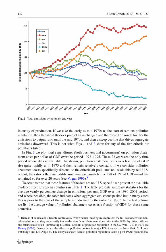
In Fig. 2 we plot the corresponding emission levels for these same pollutants over thesame time period. Figure 2 shows a general tendency for emissions to at first rise and thenfall over time. Since US income per capita grew substantially over this period, the time scalein the figure could just as well be replaced by income per capita, and hence it offers a strongconfirmation of the EKC as found, for example, by Grossman and Krueger (1994, 1995).The EKC pattern is visible in the data for all pollutants except nitrogen oxides that wereapproaching a peak, particulates which peaked before the sample period, and carbon dioxidewhich continued to grow until the 2008 recession.

It is clear however that the reduction in emission intensities shown in Fig. 1 precede thepeak level of pollutants in Fig. 2 by 25 years for sulfur dioxide, carbon monoxide, and vola-tile organic compounds. Particulates have however been falling throughout, but the peak fornitrogen oxides occurs almost 50 years after their emissions per unit output started to decline.Carbon emissions did not peak during the sample period, despite the reduction in the carbon

Footnote 7 continuedeffects and give us a clean 50 year period. Because prior to 1985 fugitive dust sources and other miscellaneousemissions were not included in PM10 we have removed these components to make the data comparable overtime. Trends reports subsequent to 1998 do not include these long consistent historical series. As well, thetrends report warns that data prior to 1970 reflect a different methodology; hence the kinks at 1970 may bedue to this change.

123

132 J Econ Growth (2010) 15:127–153

Fig. 2 Total emissions by pollutant and year

intensity of production. If we take the early to mid 1970s as the start of serious pollutionregulation, then threshold theories predict an unchanged and therefore horizontal line for theemissions to output ratio until the mid 1970s, and then a steep decline that drives aggregateemissions downward. This is not what Figs. 1 and 2 show for any of the five criteria airpollutants listed.

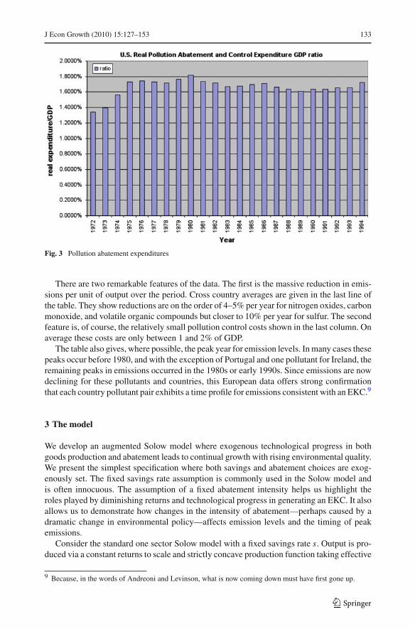
In Fig. 3 we plot total expenditures (both business and government) on pollution abate-ment costs per dollar of GDP over the period 1972–1995. These 23 years are the only timeperiod where data is available. As shown, pollution abatement costs as a fraction of GDPrise quite rapidly until 1975 and then remain relatively constant. If we consider pollutionabatement costs specifically directed to the criteria air pollutants and scale this by real U.S.output, the ratio is then incredibly small—approximately one half of 1% of GDP—and hasremained so for over 20 years (see Vogan 1996).8

To demonstrate that these features of the data are not U.S. specific we present the availableevidence from European countries in Table 1. The table presents summary statistics for theaverage yearly percentage change in emissions per unit GDP over the 1980–2001 period;and where possible, the table indicates when aggregate emissions peaked but in many casesthis is prior to the start of the sample as indicated by the entry “<1980”. In the last columnwe list the average value of pollution abatement costs as a fraction of GDP for these samecountries.

8 There is of course considerable controversy over whether these figures represent the full cost of environmen-tal regulation, and they necessarily ignore the significant abatement done prior to the 1970s by cities, utilities,and businesses.For an illuminating historical account of pollution regulation in the US from 1940 to 1970 seeDewey (2000). Dewey details the efforts at pollution control in major US cities such as New York, St. Louis,Pittsburgh and Los Angeles. The analysis shows serious pollution regulation is not a post 1970s phenomena.

123

J Econ Growth (2010) 15:127–153 133

Fig. 3 Pollution abatement expenditures

There are two remarkable features of the data. The first is the massive reduction in emis-sions per unit of output over the period. Cross country averages are given in the last line ofthe table. They show reductions are on the order of 4–5% per year for nitrogen oxides, carbonmonoxide, and volatile organic compounds but closer to 10% per year for sulfur. The secondfeature is, of course, the relatively small pollution control costs shown in the last column. Onaverage these costs are only between 1 and 2% of GDP.

The table also gives, where possible, the peak year for emission levels. In many cases thesepeaks occur before 1980, and with the exception of Portugal and one pollutant for Ireland, theremaining peaks in emissions occurred in the 1980s or early 1990s. Since emissions are nowdeclining for these pollutants and countries, this European data offers strong confirmationthat each country pollutant pair exhibits a time profile for emissions consistent with an EKC.9

3 The model

We develop an augmented Solow model where exogenous technological progress in bothgoods production and abatement leads to continual growth with rising environmental quality.We present the simplest specification where both savings and abatement choices are exog-enously set. The fixed savings rate assumption is commonly used in the Solow model andis often innocuous. The assumption of a fixed abatement intensity helps us highlight theroles played by diminishing returns and technological progress in generating an EKC. It alsoallows us to demonstrate how changes in the intensity of abatement—perhaps caused by adramatic change in environmental policy—affects emission levels and the timing of peakemissions.

Consider the standard one sector Solow model with a fixed savings rate s. Output is pro-duced via a constant returns to scale and strictly concave production function taking effective

9 Because, in the words of Andreoni and Levinson, what is now coming down must have first gone up.

123

134 J Econ Growth (2010) 15:127–153

Table 1 European evidence

Country NOx Peak SOx Peak CO Peak VOC Peak θ Share

Austria −2.8 <1980 −13.4 <1980 −5.5 <1980 −4.2 1990 1.6

Finland −3.8 1990 −11.6 <1980 −2.9 <1980 −3.8 1990 1.4

Czech Rep. −7.6 <1980 −18.6 1985 −4.8 1990 −6.5 1990 2.0

France −3.8 <1980 −10.0 <1980 −6.4 <1980 −4.2 1985 1.2

Germany −5.4 <1980 −3.1 <1980 −7.0 <1980 −2.6 1985 1.6

Italy −2.7 1990 −9.5 <1980 −3.7 1990 −3.8 1995 0.9

Ireland −2.7 2000 −7.8 <1980 −7.0 1990 −6.3 1990 0.6

Poland −7.5 1985 −9.9 1985 −10.1 1990 −6.6 <1980 1.6

Slovak Rep. −4.7 1990 −10.0 <1980 −4.2 1990 −7.5 1985 1.5

Sweden −4.2 1985 −12.1 <1980 −3.4 1990 −5.1 1985 1.0

Switzerland −4.4 1985 −9.5 <1980 −6.9 <1980 −5.1 1985 2.1

Netherlands −4.1 1985 −10.6 <1980 −6.5 <1980 −6.1 <1980 1.7

Hungary −3.0 <1980 −7.7 <1980 −3.7 <1980 −2.3 1985 0.6

Portugal 1.0 2000 −2.5 1999 −3.4 1995 1.1 1997 0.6

UK −4.5 <1980 −9.4 <1980 −5.9 <1980 −4.9 1990 1.5

Average −4.0 – −9.7 – −5.4 – −4.5 – 1.3

Notes Entries under specific pollutant headings represent the average annual percentage reduction in emis-sions per unit of real GDP over the 1980–2000 period. Dates listed under the heading “Peak” indicate theyear when emission levels peaked, with <1980 implying a peak prior to 1980. Table 1 is constructed usingthree data sources. Data on European pollution emissions comes from the monitoring agency for LRTRAPavailable at http://www.emep.int/. Real GDP data is taken from the World Bank’s Development Indicators2002 on CD Rom. Entries under θ represent pollution abatement costs as a fraction of national income. Theyare constructed from the 1996 and 2003 OECD publications “Pollution abatement and control expendituresin OECD countries”, Paris: OECD Secretariat. See the Appendix to Brock and Taylor (2004) for details onconstruction

labor and capital to produce output, Y . Capital accumulates via savings and depreciates atrate δ. The rate of labor augmenting technological progress is given by gB .

Y = F(K , BL),•K = sY − δK (1)

•L = nL ,

•B = gB B

where B represents labor augmenting technological progress and n is population growth.To model the impact of pollution we follow Copeland and Taylor (1994) by assuming every

unit of economic activity, F , generates � units of pollution as a joint product of output.10

The amount of pollution released into the atmosphere will differ from the amount producedif there is abatement. We assume abatement is a constant returns to scale activity and writethe amount of pollution abated as an increasing and strictly concave function of the totalscale of economic activity, F , and the economy’s efforts at abatement, F A. If abatement atlevel A, removes the �A units of pollution from the total created, then we have pollutionemitted equals pollution created minus pollution abated, or:

10 This approach has been subsequently employed by many authors (Stokey 1998; Aghion and Howitt 1998,etc.). In these other papers, � is taken as constant over time and by choice of units set to one. Some authors(for e.g., Stokey 1998) who adopt this approach refer to the firm’s or planner’s problem as one of choosingacross dirty or clean technologies rather than less or more abatement. These approaches are identical.

123

J Econ Growth (2010) 15:127–153 135

E = �F − �A(F, F A)

E = �F[1 − A(1, F A/F)

](2)

E = �Fa(θ),

where a(θ) ≡[1 − A(1, F A/F)

]and θ = F A/F

where the second line follows from the linear homogeneity of A, and the third by the definitionof θ as the fraction of economic activity dedicated to abatement. We assume the intensiveabatement function satisfies a(0) = 1 and note a′(θ) < 0 and a′′(θ) > 0 by concavity.Abatement has a positive but diminishing marginal impact on pollution reduction. In somecases we will adopt the specific form a(θ) = (1 − θ)ε where ε > 1.

To combine our assumptions on pollution and abatement with the Solow model, we notethat taking abatement into account, output available for consumption or investment Y , thenbecomes Y = [1 − θ ]F . And to match the Solow model’s exogenous technological progressin goods production raising effective labor at rate gB , we assume exogenous technologicalprogress in abatement lowering � at rate gA > 0. Transforming our measures of output,capital and pollution into intensive units, we obtain:

y = f (k)[1 − θ ] (3)•k = s f (k)[1 − θ ] − [δ + n + gB ]k (4)

e = f (k)�a(θ) (5)

where k = K/BL , y = Y/BL , e = E/BL and f (k) = F(k, 1).

3.1 Balanced growth path

Assume the Inada conditions hold for F , then with θ fixed it is immediate that starting fromany k(0) > 0, the economy converges to a unique k∗ as in the Solow model. As the economyapproaches its balanced growth path, aggregate output, consumption and capital all grow atrate gB + n while their corresponding per capita magnitudes grow at rate gB . Using standardnotation for growth in per capita magnitudes, along the balanced growth path we must havegy = gk = gc = gB > 0. A potentially worsening environment however threatens thishappy existence. Since k approaches the constant k∗ we can infer from (5) that the growthrate of aggregate emissions along the balanced growth path, gE , is given by:

gE = gB + n − gA (6)

The first two terms in (6) represent the scale effect of growth on emissions since aggregateoutput grows at rate gB + n along the balanced growth path. The second term is a techniqueeffect created by technological progress in abatement.

Define sustainable growth as a balanced growth path generating both rising consumptionper capita and an improving environment. Sustainable growth is guaranteed by:

gB > 0 and gA > gB + n (7)

Technological progress in goods production is necessary to generate per capita incomegrowth. Technological progress in abatement must exceed growth in aggregate output inorder for pollution to fall and the environment to improve.

123

136 J Econ Growth (2010) 15:127–153

3.2 Diminishing returns and the EKC

The Green Solow model, although simple, generates a very suggestive explanation for muchof the empirical evidence relating income levels to environmental quality. Despite the factthat the intensity of abatement is fixed, there are no composition effects in our one goodframework, and no political economy or intergenerational conflicts to resolve, the GreenSolow model produces a path for income per capita and environmental quality that traces outan EKC.11 This is not to suggest that the EKC pattern we have seen in the U.S. or Europeandata is necessarily independent of policy choices made in those regions, but rather that atightening of policy per se is not required for the result.

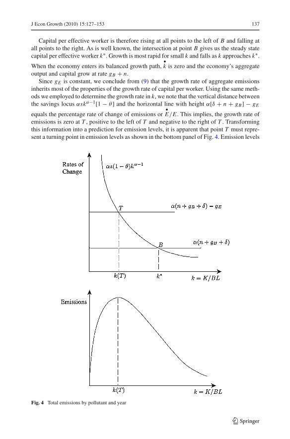
To demonstrate we use the two panels in Fig. 4. The top panel plots the growth rate ofemissions and capital against capital per effective labor and is very similar to graphical rep-resentations of the Solow model. The second follows from the first and plots the level ofemissions as a function of capital per effective worker and is very similar to representationsof the EKC. To start we need to develop a differential equation for emissions. To generateclosed form solutions, we adopt a Cobb-Douglas formulation with a constant capital shareα, with 0 < α < 1 as this allows us to write emissions at any time t as:12

E = B(0)L(0)�(0)a(θ) exp[gE t]kα (8)

where B(0), L(0), and �(0) are initial conditions, and use has been made of (2), (6), andthe linear homogeneity of F . Differentiate with respect to time to obtain the growth rate ofemissions:

•E

E= gE + α

•k

k(9)

where we note the rate of change of capital per effective worker is simply:

•k

k= skα−1(1 − θ) − (δ + n + gB) (10)

Using these two expressions we can now link the dynamics of capital accumulation to theevolution of pollution levels using the two panels of Fig. 4.

In the top panel of Fig. 4 we plot on the vertical axis the rates of change of (α times)

capital per effective worker α•k/k and aggregate emissions

•E/E , and on the horizontal axis

capital per effective worker k. In drawing the figure we have implicitly assumed growth issustainable: i.e., gE < 0. We refer to the negatively sloped line given by αskα−1[1 − θ ]as the savings locus since it shifts with the savings rate s. The savings locus starts at plusinfinity and approaches zero as k grows large; therefore, it must intersect the two horizontallines as shown by points T and B. From (10) it is clear that the vertical distance betweenαskα−1[1 − θ ] and the horizontal line with height α[δ + n + gB] is just α times the growth

rate of capital per effective worker or α•k/k.

11 For example, although we take θ as exogenous and independent of other model features, it is likely thattighter regulation spurs technological progress in abatement and hence is related to our primitive gA . Forempirical evidence along these lines see the recent survey by Popp et al. (2009). Xepapadeas (2005) also notesthat technological progress in abatement can generate an EKC pattern. His discussion is brief and appears ina review article as does our first discussion of Green Solow in Brock and Taylor (2005).12 The constant capital share assumption lets us solve for the evolution of k(t) explicitly, but has no impacton the results in general.

123

J Econ Growth (2010) 15:127–153 137

Capital per effective worker is therefore rising at all points to the left of B and falling atall points to the right. As is well known, the intersection at point B gives us the steady statecapital per effective worker k∗. Growth is most rapid for small k and falls as k approaches k∗.

When the economy enters its balanced growth path,•k is zero and the economy’s aggregate

output and capital grow at rate gB + n.Since gE is constant, we conclude from (9) that the growth rate of aggregate emissions

inherits most of the properties of the growth rate of capital per worker. Using the same meth-ods we employed to determine the growth rate in k, we note that the vertical distance betweenthe savings locus αskα−1[1 − θ ] and the horizontal line with height α[δ + n + gB] − gE

equals the percentage rate of change of emissions or•E/E . This implies, the growth rate of

emissions is zero at T , positive to the left of T and negative to the right of T . Transformingthis information into a prediction for emission levels, it is apparent that point T must repre-sent a turning point in emission levels as shown in the bottom panel of Fig. 4. Emission levels

Fig. 4 Total emissions by pollutant and year

123

138 J Econ Growth (2010) 15:127–153

are rising to the left of T and falling to the right of T . Under the assumption that growth issustainable, gE < 0, and point T lies to the left of B: the model generates the EKC profileshown in the lower panel.

The figure illustrates several features of the model. It shows that if growth is sustainablethen T lies to the left of B and the time profile for emission levels depends on the location ofk(0) relative to point T . If an economy starts with a small initial capital stock then emissionsat first rise and then fall as development proceeds: i.e. we obtain a hump-shaped EKC profilefor emissions. If initial capital is larger it is possible that the level of emissions falls mono-tonically as the economy moves towards its sustainable growth path. When emissions peakdepends on the relationship between points T and B. For example, if −gE is small, then Tand B differ very little and emissions will only peak as the economy approaches its balancedgrowth path which may of course take a very long time. When growth is not sustainable Tlies to the right of B and emissions will grow forever even as the economy approaches itsbalanced growth path. In all cases, the economy’s intensity of abatement is constant, and itsemissions to output ratio falls—both in and out of steady state—at the constant rate −gA.

It is important to note while the model allows for the possibility that emissions may atfirst rise and then fall, or they may fall continuously or rise continuously, the growth rate ofemissions is monotonically declining in k. This is true because the growth rate of emissionsis very rapid for countries a long way from point B, and slower for those near B. Even inthe unsustainable case, the growth rate of emissions falls along the transition path until itapproaches its balanced growth path rate from above. We will exploit this property later whenwe derive an estimating equation predicting convergence in emissions across countries. Werecord these results as a proposition.

Proposition 1 If growth is sustainable and k(T ) > k(0), then the growth rate of aggre-gate emissions is at first positive but turns negative in finite time. If growth is sustainable andk(0) > k(T ), then the growth rate of emissions is negative for all t. If growth is unsustainable,then emissions growth declines with time but remains positive for all t.

Proof See Appendix

Proposition 1 tells us about the shape of the emissions profile but says very little aboutthe level of emissions and the level of income per capita at the turning point T . Although themodel is simple, it can be deceptive in this regard. For example, it is a short step from know-ing that k(T ) is unique to a belief that income per capita at the turning point is also unique.Similarly, it is easy to assume that the peak emissions level is the same for countries sharingsavings rates, population growth rates, etc. Both of these conjectures are wrong: althoughk(T ) is unique, the associated income per capita and emissions level at k(T ) are not. ��Proposition 2 Economies with identical parameter values but different initial conditionsproduce different income per capita and emission profiles over time. The peak level of aggre-gate emissions and the level of income per capita associated with peak emissions are notunique.

Proof in text below.

Proposition 2 offers a simple explanation for the apparent inconsistency between the obser-vation of an EKC in country level data and the fragility of cross-country empirical results.It is now well known that the shape of the estimated EKC can differ quite widely whenresearchers vary the time period of analysis, the sample of countries, the pollutant, or even

123

J Econ Growth (2010) 15:127–153 139

the data source. For example, Harbaugh et al. (2002) reconsider Grossman and Krueger’sspecification and find little support for an EKC using newer updated data. Stern and Common(2001) employ a larger and different sulfur dioxide dataset and find no EKC. And the lit-erature reviews by both Barbier (1997) and Stern (2004) note that published work differsgreatly in the estimated turning points for the EKC, the standard errors on turning points arevery large, and the results differ widely across pollutants and countries. Criado (2008) comesto similar conclusions. At the same time, plots of raw pollution data for the US and othercountries often present a dramatic confirmation of the EKC.

If EKC profiles for even very similar countries are not unique because of differences ininitial conditions, then unobserved heterogeneity is surely a problem. Unobserved heteroge-neity could then account for the large standard errors on turning points and the sensitivity ofresults to the sample. ��

3.3 Turning points

To examine the determinants of emissions and income per capita at the peak, we start bywriting income per capita at any time t as:

yc(t) = [1 − θ ]k(t)α B(0) exp[gBt] (11)

which is a function of k(t), time t , the intensity of abatement θ , and the initial conditionB(0). Denote by t = T , the calendar time at which emissions reach their peak. At t = T ,the economy’s capital per effective worker reaches k(T ). To solve for the k(T ) identified inFig. 4, substitute (10) into (9) and set it to zero to find:

k(T ) =[

s(1 − θ)

n + gB + δ − gE/α

]1/(1−α)

(12)

Next solve the differential equation in (10) to find:

k(t) =[k∗(1−α)(1 − exp[−λt]) + k(0)(1−α) exp[−λt]

]1/(1−α)

(13)

As expected k(t) is an exponentially weighted average of initial capital per worker k(0)

and its balanced growth path level k∗ where the weight given to initial versus final positionsis determined by the speed of adjustment λ = [1 − α][n + gB + δ] and time t . k∗ is foundby setting (10) to zero to find k∗ = [[s(1 − θ)]/[n + gB + δ]]1/(1−α). Finally, we now setk(t) equal to k(T ) to find an implicit equation for the time it takes to reach the peak level ofemissions. T is defined by:

T : k(T ) =[k∗(1−α)(1 − exp[−λT ]) + k(0)(1−α) exp[−λT ]

]1/(1−α)

(14)

where k(0) = K (0)/B(0)L(0). Rearranging (14) we find:

T = 1

λlog

[k∗(1−α) − k(0)1−α

k∗(1−α) − kT (1−α)

](15)

The calendar time needed to reach peak emissions is declining in the convergence speedof the Solow model, λ, increasing in the gap between initial and final capital per effectiveworker, and is larger the closer is point T to B. Peak emission levels follow similarly. Puttingall this together we can now write income per capita at the peak as:

yc(T ) = [1 − θ ][k(T )]α B(0) exp[gB T ] (16)

123

140 J Econ Growth (2010) 15:127–153

Income per capita at the peak is rising in capital per effective worker at the peak, and risingin the calendar time T needed to reach the peak.

To find peak emissions we use (13) and (8) to find:

E(t) = c0 exp[gE t][[

k∗(1−α)(1 − exp[−λt]) + k(0)(1−α) exp[−λt]]α/(1−α)

]

c0 = B(0)L(0)�(0)a(θ) (17)

and hence peak emissions are just:

E(T ) = c0 exp[gE T ] [k(T )]α (18)

Peak emissions are rising in the capital intensity of the economy, and when growth is sus-tainable they are falling in the time to reach peak emissions.

It is now easy see that if we compare two economies with the same parameters—savingsrate, population growth rates, rate of depreciation, rates of technological progress, and capitalshare—and hence the same k∗, these economies will not share the same income per capitalevel at their peak level of emissions, nor will they share the same peak level of emissions.

The logic is straightforward although lengthy. Peak emissions are reached when the rateat which emissions are created via output growth is exactly offset by the rate at which theyare abated. The share of output allocated to abatement as an input is constant over time, buttechnological progress in abatement is raising the effectiveness of these inputs at the con-stant rate gA. The rate at which emissions are created declines monotonically as the economyapproaches its balanced growth path; the rate of technological progress in abatement is con-stant. Therefore, the time T at which these two rates equalize is determined by how far initialcapital per effective worker is from its eventual steady state. The further is initial capitalfrom its steady state, the faster is economic growth and the longer it is before the growth inemissions hits zero.

This logic tells us that the time to peak emissions, T , is longer the smaller is k(0), but Titself is independent of any variation in initial conditions that leaves k(0) unchanged. Con-sequently if we alter initial conditions slightly by raising the effectiveness of labor in periodzero, B(0), but make compensating changes in the labor force or initial capital stock to leavek(0) unchanged, then we will have left T unchanged. But carrying this thought experimentforward we know that since labor is more productive to start with, income per capita at thepeak level of emissions is now higher than otherwise. An exactly analogous argument canbe used to show that peak emissions are not unique. Since �(0) plays no role in determiningk(T ) or T ; variations in it alter the peak level of emissions directly via (8).

Since empirical work relates income per capita to emissions and not time as we have here,it is useful to make the connection between our theory and the existing empirical work pre-cise. To do so we note from (13) and (11) that yc(t) is a strictly increasing function of time.We can therefore invert it finding t = φ(yc) and substitute for time in (17). This gives usa parametric relationship between aggregate emissions and income per capita. Establishingthe properties of this relationship requires further work that we leave to the appendix, but wenote here:

Proposition 3 There exists a parametric relationship between aggregate emissions E andincome per capita yc that we refer to as an EKC. If k∗ > k(T ) > k(0), then emissionsfirst rise and then fall with income per capita. If k∗ > k(0) > k(T ), then emissions fallmonotonically with income per capita.

Proof See Appendix

123

J Econ Growth (2010) 15:127–153 141

3.4 Comparative steady state analysis

Most of the empirical work investigating the EKC employs cross country data that includesboth developed and developing countries and often both democratic and communist states.Clearly these economies differ in much more than just initial conditions, and this hetero-geneity may further confound estimation. To investigate how differences across countriesin savings, abatement and rates of technological progress affect emissions growth, we nowconduct a comparative steady state analysis.

Consider the role of savings. A change in the savings rate has no effect on the long rungrowth rate of emissions or output, but it can have an impact on transitional growth and hencean economy’s income pollution path. An increase in the savings rate shifts the savings locusrightward raising both T and B in Fig. 4. Greater savings raises capital per effective workerin steady state and capital per effective worker at the turning point. If we substitute for k∗and k(T ) in (15) it is possible to show that an increase in the savings rate lengthens the timeto peak emissions, T . Therefore, an economy with a higher savings rate reaches its peakemissions level at a higher income per capita than otherwise. The intuition is simple. Theturning point for emissions rises because higher savings implies more rapid capital accumu-lation. This in turn means faster output growth and faster emissions growth at any given k.The turning point in emissions is reached when diminishing returns to capital accumulationlowers output growth to such an extent that it now equals −gA. A higher savings rate makesthis task harder, and hence k(T ) and T rises.

An increase in abatement intensity has quite interesting impacts. Given the prominent rolepolicy changes have played in explanations for the EKC, but not in the formulation presentedhere, it is important to discuss these impacts at some length. It is clear that a change in theintensity of abatement has no long run impact on the economy’s growth rate in terms ofoutput or emissions, just as differences in savings rates have no long run impact. To verifythis inspect (17). In the long run, the path for aggregate emissions is fully determined by itsgrowth rate, gE , and its level which is set by initial conditions, k∗, and a(θ). A permanentchange in policy that raises θ , lowers the entire path of emissions by lowering the capitalintensity of the economy and hence output at every t , lowering emissions per unit outputbecause the policy requires cleaner techniques, but it does not affect the long run growth rateof emissions.

Within the confines of the Green Solow model, tighter policy that raises θ cannot turn anunsustainable growth path into a sustainable one.13 But this does not mean that policy hasno impact on emissions growth, incomes or turning points. Tighter policy creates a policyinduced drag on transitional growth, and this affects everything. To see why note that anincrease in abatement lowers (1 − θ) and shifts the savings locus leftward thereby loweringboth T and B. Using (15) we find the time to peak emissions T falls. Therefore, a higherabatement intensity implies that peak emissions are reached at a lower level of income percapita than otherwise; the peak in emissions is reached earlier than otherwise, and emissionlevels are lower. Interestingly, emissions start their decline at a lower income per capita notbecause abatement is effective in lowering the level of emissions (although it does do thisin a level sense), but because abatement uses up scarce resources that would otherwise havegone to investment and spurred growth. A higher intensity of abatement, creates a policyinduced drag on the rate of transitional growth and it is this impact that lowers k(T ). So, eventhough a permanent change in abatement intensity has no long run effect on emission growth

13 If the increase in costs created by the policy leads to innovation raising gA , then policy could have longrun impacts.

123

142 J Econ Growth (2010) 15:127–153

rates, it does affect the time profile for emissions and income. Since the policy change lowersthe level of pollution, research studying its impact could correctly find it effective in low-ering pollution, while raising firms costs and perhaps bringing forward a peak in emissionsoverall.14

Finally, consider the impact of changes in technological progress. Start with changes inthe rate of progress in abatement, gA. An increase in gA, shifts the top line in Fig. 4 upwardslowering k(T ). This lowers the growth rate of emissions for any k, and likewise lowers thegrowth rate of emissions in steady state. This change has no effect on the growth rate ofoutput or on k∗. Using (15) we find T is reduced. Putting these results together we find peakemissions are reached at a lower income per capita than otherwise and earlier than otherwise.

Faster technological progress in goods production has less clear cut effects. An increasein gB shifts the top line in Fig. 4 downward raising T and the bottom line upwards loweringB. The growth rate of aggregate emissions rises at any k, while the growth rate of capital perworker falls at any k. The time to peak emissions could rise or fall, and hence income percapita at the peak may be higher or lower.

A similar result arises from changes in population growth. Population growth lowerssteady state capital per worker and this lowers transitional growth in capital per worker atany given k. But population growth raises emissions directly via a scale effect and this raisesboth emissions growth and the point at which emissions start to fall. Whether this new highertransition point is reached sooner or later in calendar time is indeterminate and hence so toois the associated income per capita.

These results demonstrate that relationship between income and pollution is exceedinglycomplex in even this the simplest of models. We have in fact identified three qualitativelydifferent sets of determinants. The first set of determinants are initial conditions (B(0) and�(0)) that affect the transition paths for emissions and income but have no effect on steadystate magnitudes nor long run growth rates. A second set of determinants (s and θ ) affectthe transition paths for emissions and income and change steady state magnitudes, but haveno impact on long run growth rates. The final set of determinants (gB , n, and gA) affect thetransition paths for emissions and income, change steady state magnitudes, and alter longrun growth rates of output and emissions.

4 Empirical methodology

While many authors have been critical of the EKC methodology, very little has been offeredas a productive alternative. In this section we present an alternative method to investigate thegrowth and environment relationship that draws on existing work in macroeconomics.

The Green Solow model contains two empirical predictions regarding convergence inemissions. The first is that a group of countries sharing the same parameter values—savingsrates, abatement intensities, rates of technological progress etc.—but differing in initial con-ditions will exhibit convergence in a measure of their emissions. This is true even thougheach of these countries would typically exhibit a unique income and pollution profile overtime. We will derive an estimating equation below to show that under the assumption ofidentical parameters values across countries, the model predicts Absolute Convergence inEmissions per capita or ACE. The second prediction is that in a world with heterogenous

14 For research documenting the impact of the Clean Air Act Amendments on economic activity and pollu-tion concentrations see Becker and Henderson (2000) for ozone, Chay and Greenstone (2005) for particulatematter, and Greenstone (2004) for sulfur dioxide.

123

J Econ Growth (2010) 15:127–153 143

countries we will need to condition on the right country characteristics to find what we willrefer to as Conditional Convergence in Emissions per capita or CCE.

4.1 Estimating equation

We start with Eq. 8 for emissions but rewrite it in terms of emissions per capita ec(t) =E(t)/L(t), and income per capita, yc(t) = F(t)[1 − θ ]/L(t). Using standard notation, thisgives us:

ec(t) = �(t)a(θ̃)yc(t) (19)

where a(θ̃) = a(θ)/[1 − θ ]. Differentiating with respect to time yields

•ec

ec= −gA +

•yc

yc(20)

As shown, growth in emissions per capita is the sum of technological progress in abate-ment plus growth in income per capita. We transform (20) into our estimating equation inthree steps. First approximate the growth rate of income per capita and emissions per capitaover a discrete time period of size N by their average log changes and rewrite the equationas:

[1/N ] log[ect /ec

t−N ] = −gA + [1/N ] log[yct /yc

t−N ] (21)

To eliminate income growth, we follow Mankiw et al. (1992) and Barro (1991) and approx-imate the discrete N period growth rate of income per capita near the model’s steady statevia a log linearization to obtain:15

[1/N ] log[yct /yc

t−N ] = b − [1 − exp[−λN ]]N

log[yct−N ] (22)

where b is a constant (discussed in more detail below) and λ = [1 − α][n + gB + δ] is theSolow model’s speed of convergence towards k∗.

Finally substitute for income growth in (21) using (22) and eliminate initial period incomeper capita using yc

t−N = et−N /�t−N a(θ̃) from Eq. 19.By making these substitutions we obtain a simple linear equation relating changes in

emissions per capita across i countries (over a discrete period of length N ) to a constant andinitial period emissions per capita. Since individual elements making up the constant term arenot identified we have no prediction concerning the sign. The growth rate of emissions percapita should however fall with higher initial period emissions per capita. Ceterus paribus,a lower emissions per capita ec

t−N corresponds to a lower initial capital per effective workerkt−N . This then implies a rapid rate of growth in aggregate emissions E and hence a rapidrate of growth of emissions per capita. We write this short specification as a simple linearregression with error term μi t .

[1/N ] log[ecit/ec

it−N ] = β0 + β1 log[ecit−N ] + μi t (23)

Somewhat heroic assumptions are needed to estimate (23) consistently with OLS. Forexample, if we assume countries share the same steady state y∗, then countries can differonly in their initial, and largely unobservable, technology levels �t−N and Bt−N . Mankiw etal. (1992) address this concern by assuming the initial goods technology Bt−N differs acrosscountries by at most a idiosyncratic error term. This assumption has however come under

15 See our discussion paper Brock and Taylor (2004) for a full derivation.

123

144 J Econ Growth (2010) 15:127–153

severe criticism on both econometric and theoretical grounds (see especially Durlauf andQuah (1999)). One concern is that unobserved variation in initial technologies Bi,t−N acrossi may be correlated with ec

it−N . For example a technologically sophisticated country with alarge Bi,t−N may have greater emissions per capita by virtue of its greater output per capita.

While unobserved heterogeneity is certainly a possibility, it may pose less of a problemin our context. The reason is simply that a productive goods technology implies a largeinitial Bt−N , while a productive emissions technology implies a small �t−N . Therefore, atechnologically sophisticated country at T − N may have the same �i,t−N Bi,t−N as a techno-logically backward country at T − N making unobserved heterogeneity in initial technologylevels less of a problem. In some circumstances this heuristic argument is exact. Assumeinitial technology levels are proportional to each country’s initial “technological sophisti-cation” at T − N . Denote technological sophistication by Si,t−N then �i,t−N = α/Si,t−Nand Bi,t−N = βSi,t−N for some α and β positive. Under this assumption, the product,�i,t−N Bi,t−N = αβ, is independent of i .

We invoke this argument to justify a decomposition of the unobservable country specificproducts �i,t−N

Bi,t−N into an overall cross country mean we denote by_______

�t−N Bt−N plus

a country specific deviation.16 We assume these country specific deviations, plus standardapproximation error in generating our linear form, ηit are contained in our error term μi t asshown below in our long specification. OLS is consistent if the covariance of μi t and ourright hand side variables is zero.

To generate the long specification we need to unbundle the determinants of the steadystate. Before doing so, we should be specific about how our empirical method accounts forthe three different sets of variables that determine emissions growth. First, as is commonto the growth literature, we assume that rates of technological progress are common world-wide.17 In addition, we condition on population growth rates.18 Therefore, the set of factorsthat determines both steady states and the rate of growth along the balanced growth path areaccounted for by either assumption or measurement.

Second, the long specification allows us to condition on abatement and savings, althoughabatement in the case of carbon (over this period of time) is effectively zero. Therefore, theset of factors that affect only steady state magnitudes are controlled for in the regression.

Finally, under our assumption that a country’s initial technological sophistication acrossboth abatement and production technologies are related, we have reduced the across-coun-try variation in initial conditions. Therefore, under this assumption, differences in initialconditions are accounted for in the estimation.

To generate our long specification it proves useful to adopt as the specific form of theabatement function a(θ) = (1 − θ)ε where ε > 1. This formulation follows from a constantreturns abatement function, and like all iso-elastic functions it is quite useful in empiricalwork. Then letting si , θi , and (n + gB + δ)i be the time-averaged country specific savingsrate, abatement intensity and effective depreciation rate respectively, and substituting for thedeterminants of y∗ we write the long specification as:

16 The interested reader should note that even when countries share parameter values and satisfy this meantechnology requirement, their income pollution profiles are still not unique making EKC estimation problem-atic.17 See Stern (2005, 2007) for an approach allowing for country specific rates of technological progress inabatement technology.18 We also follow the literature by ignoring the reliance of λ on population growth rates and estimate a linearspecification.

123

J Econ Growth (2010) 15:127–153 145

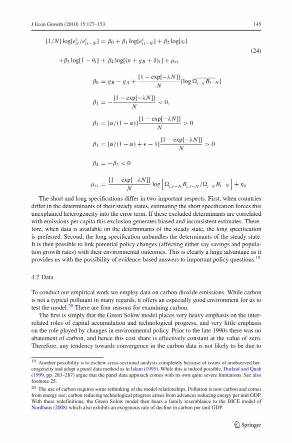
[1/N ] log[ecit/ec

it−N ] = β0 + β1 log[ecit−N ] + β2 log[si ]

(24)

+β3 log[1 − θi ] + β4 log[(n + gB + δ)i ] + μi t

β0 = gB − gA + [1 − exp[−λN ]]N

[log________

�t−N Bt−N ]

β1 = −[1 − exp[−λN ]]N

< 0,

β2 = [α/(1 − α)] [1 − exp[−λN ]]N

> 0

β3 = [α/(1 − α) + ε − 1] [1 − exp[−λN ]]N

> 0

β4 = −β2 < 0

μi t = [1 − exp[−λN ]]N

log[�i,t−N Bi,t−N /

________�t−N Bt−N

]+ ηit

The short and long specifications differ in two important respects. First, when countriesdiffer in the determinants of their steady states, estimating the short specification forces thisunexplained heterogeneity into the error term. If these excluded determinants are correlatedwith emissions per capita this exclusion generates biased and inconsistent estimates. There-fore, when data is available on the determinants of the steady state, the long specificationis preferred. Second, the long specification unbundles the determinants of the steady state.It is then possible to link potential policy changes (affecting either say savings and popula-tion growth rates) with their environmental outcomes. This is clearly a large advantage as itprovides us with the possibility of evidence-based answers to important policy questions.19

4.2 Data

To conduct our empirical work we employ data on carbon dioxide emissions. While carbonis not a typical pollutant in many regards, it offers an especially good environment for us totest the model.20 There are four reasons for examining carbon.

The first is simply that the Green Solow model places very heavy emphasis on the inter-related roles of capital accumulation and technological progress, and very little emphasison the role played by changes in environmental policy. Prior to the late 1990s there was noabatement of carbon, and hence this cost share is effectively constant at the value of zero.Therefore, any tendency towards convergence in the carbon data is not likely to be due to

19 Another possibility is to eschew cross-sectional analysis completely because of issues of unobserved het-erogeneity and adopt a panel data method as in Islam (1995). While this is indeed possible, Durlauf and Quah(1999, pp. 283–287) argue that the panel data approach comes with its own quite severe limitations. See alsofootnote 25.20 The use of carbon requires some rethinking of the model relationships. Pollution is now carbon and comesfrom energy use; carbon reducing technological progress arises from advances reducing energy per unit GDP.With these redefinitions, the Green Solow model then bears a family resemblance to the DICE model ofNordhaus (2008) which also exhibits an exogenous rate of decline in carbon per unit GDP.

123

146 J Econ Growth (2010) 15:127–153

convergence in say environmental policy across countries. In this sense, carbon is an espe-cially clean case to test the forces highlighted by the Green Solow model.

Second, it is virtually impossible to obtain reliable cross-country data on pollution emis-sions from a broad spectrum of countries over any considerable length of time. The GlobalEnvironment Monitoring system offers us reliable data on pollution concentrations world-wide since the mid 1970s, but obtaining similar data on emissions is not possible. Thisis clearly a problem. Identifying the impact of differences in savings rates and populationgrowth rates on emissions requires significant cross country variation in the data, and anycredible test of convergence requires data over long periods of time. Carbon data is availablefor a broad spectrum of countries over lengthy periods of time.21

Third, researchers have had great difficulty making sense of the carbon data. There ismuch disagreement over whether carbon emissions per capita are converging or divergingworldwide.22 Understanding the dynamics of carbon is also critical to decisions over theappropriate response to global warming. Many of the computable models used to generatebusiness as usual trajectories assume some degree of convergence across countries; if howeveremissions per capita do not converge or converge only slowly then existing business-as-usualtrajectories may be seriously in error.

Finally, the existing evidence on European and U.S. criteria pollutants shows that pollu-tion emissions are falling across the board for many countries. In contrast, carbon emissionsare not trending downward. As a result, carbon offers us the opportunity to disentangle theobservation of an EKC like pattern in the data from the less restrictive prediction of conver-gence. Since convergence in emissions per capita is the key prediction of the Green Solowmodel it is useful to examine a pollutant that does not appear to follow an EKC pattern.

We collected data on carbon emissions per capita, population growth rates and the invest-ment share of GDP for a group of 173 countries from 1960 to 1998. The period ending date of1998 was selected to ensure that Kyoto commitments could have little impact on emissions.The period starting date of 1960 and the cross-country coverage was determined solely bydata limitations imposed by the Penn. World Tables and the World Development Indicatorsdatabase.

We consider five samples. Sample A contains the 173 countries with data on emissions percapita during the relevant period. We use this sample to estimate our short specification andinvestigate ACE. Sample B includes only those countries where we can evaluate CCE; i.e. theset of countries that have data on population growth and the investment share of GDP. Thisreduces the sample to 165 countries. Sample C eliminates OPEC members; while Sample D,excludes all those with a population size less than one million in 1960. Sample E, adds tothese restrictions by eliminating countries that are “not rated” by the Penn. World Tables.23

21 Data on emissions at the U.S. state level could also satisfy this requirement, but the mobility of labor andcapital across states introduces further complications.22 For recent published see Dijkgraaf et al. (2005); a very recent review is “Convergence clubs in per-capitaCO2 emissions: who’s converging who’s diverging” March 2008, Carlos Ordas Criado and Jean Marie Grether,Institute for Research in Economics, Neuchatel Switzerland, mimeo.23 A table of summary statistics for all regressors can be found in the Appendix. The exclusion of OPECand small countries from a sample is common in the empirical growth literature. For OPEC, the reason forexclusion is simply that oil extraction and not value-added activities are responsible for most of GDP. For verysmall countries, their industrial structure often reflects peculiar features such as a financial or trading entrepot.The exclusion of countries on the basis of data quality is also common.

123

J Econ Growth (2010) 15:127–153 147

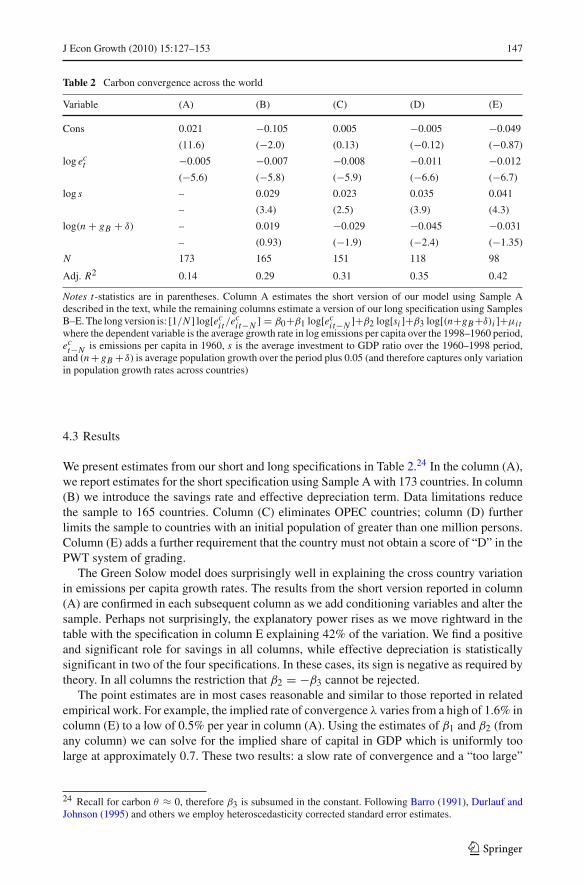
Table 2 Carbon convergence across the world

Variable (A) (B) (C) (D) (E)

Cons 0.021 −0.105 0.005 −0.005 −0.049

(11.6) (−2.0) (0.13) (−0.12) (−0.87)

log ect −0.005 −0.007 −0.008 −0.011 −0.012

(−5.6) (−5.8) (−5.9) (−6.6) (−6.7)

log s – 0.029 0.023 0.035 0.041

– (3.4) (2.5) (3.9) (4.3)

log(n + gB + δ) – 0.019 −0.029 −0.045 −0.031

– (0.93) (−1.9) (−2.4) (−1.35)

N 173 165 151 118 98

Adj. R2 0.14 0.29 0.31 0.35 0.42

Notes t-statistics are in parentheses. Column A estimates the short version of our model using Sample Adescribed in the text, while the remaining columns estimate a version of our long specification using SamplesB–E. The long version is: [1/N ] log[ec

it /ecit−N ] = β0+β1 log[ec

it−N ]+β2 log[si ]+β3 log[(n+gB+δ)i ]+μi twhere the dependent variable is the average growth rate in log emissions per capita over the 1998–1960 period,ec

t−N is emissions per capita in 1960, s is the average investment to GDP ratio over the 1960–1998 period,and (n + gB + δ) is average population growth over the period plus 0.05 (and therefore captures only variationin population growth rates across countries)

4.3 Results

We present estimates from our short and long specifications in Table 2.24 In the column (A),we report estimates for the short specification using Sample A with 173 countries. In column(B) we introduce the savings rate and effective depreciation term. Data limitations reducethe sample to 165 countries. Column (C) eliminates OPEC countries; column (D) furtherlimits the sample to countries with an initial population of greater than one million persons.Column (E) adds a further requirement that the country must not obtain a score of “D” in thePWT system of grading.

The Green Solow model does surprisingly well in explaining the cross country variationin emissions per capita growth rates. The results from the short version reported in column(A) are confirmed in each subsequent column as we add conditioning variables and alter thesample. Perhaps not surprisingly, the explanatory power rises as we move rightward in thetable with the specification in column E explaining 42% of the variation. We find a positiveand significant role for savings in all columns, while effective depreciation is statisticallysignificant in two of the four specifications. In these cases, its sign is negative as required bytheory. In all columns the restriction that β2 = −β3 cannot be rejected.

The point estimates are in most cases reasonable and similar to those reported in relatedempirical work. For example, the implied rate of convergence λ varies from a high of 1.6% incolumn (E) to a low of 0.5% per year in column (A). Using the estimates of β1 and β2 (fromany column) we can solve for the implied share of capital in GDP which is uniformly toolarge at approximately 0.7. These two results: a slow rate of convergence and a “too large”

24 Recall for carbon θ ≈ 0, therefore β3 is subsumed in the constant. Following Barro (1991), Durlauf andJohnson (1995) and others we employ heteroscedasticity corrected standard error estimates.

123

148 J Econ Growth (2010) 15:127–153

capital share are of course the same as those reported by Barro (1991) from an estimation ofthe standard Solow model.25

All together the negative coefficient on initial emissions per capita, the positive role forsavings, and the slow rate of convergence all argue that Solow type forces play a major rolein determining the growth rate of carbon emissions.26

The coefficient estimates also allow us to ask how the high investment rates and fast pop-ulation growth rates in many developing countries affect the growth rate of their emissions.For example, consider the results presented in column E. Countries within sample E had anaverage annual growth rate of emissions per capita of 1.98% per year, an average invest-ment share of 21.3%, and an average population growth rate of 1.54% per year. Consider anincrease in the investment share, s, of an “average country” by 10% points to a little over31%. In the very long run, an increase in the savings rate has no effect on emissions growthor emissions per capita growth. Outside of steady state however a higher savings rate impliesfaster interim growth to reach a new steady state with higher capital per person. Using thecoefficient estimates from column E, this 10% point increase in the savings rate would raisethe average country’s emissions growth rate by 1.57% per year. This is a significant increasesince the average growth rate of emissions per capita over the last 30 years is slightly lessthan 2% per year.

Alternatively, suppose our average country’s population growth doubled from 1.54% toa little over 3%. Again in the very long run, this increase has no effect on emissions percapita growth although it must raise overall emissions growth by 1.54%. Outside of steadystate, a faster growing population lowers capital per person, lowers labor productivity, slowsinterim growth and should slow emissions per capita growth as well. To find the magnitudeof this effect, start with our average country at the mean of the sample. Then a doubling ofpopulation growth implies a reduction in the growth rate of emissions per capita by 0.65% peryear. Emissions per capita growth falls with faster population growth, although this effect istemporary. Growth in overall emissions rises both in the transition period and forever. Duringthe transition, overall emissions rise by 0.89% per year; while rising the full 1.54% in thelong run.

Alternatively consider the thought experiment of lowering population growth to zerofrom its current mean. Emissions per capita growth would rise by 0.83%, and overallemissions growth would only fall by 0.71% per year in the interim. In the very longrun, emissions growth would fall by 1.54% but the short run out-of-steady-state impact issmall.

The purpose of this exercise and these results was to demonstrate that the forces high-lighted by the Green Solow model are significant determinants of emissions growth. Incontrast to earlier work documenting a finding of convergence in emissions growth or levels,our approach offers a potential window into the determinants of growth and the roles playedby investment, population growth and abatement behavior. Additional empirical work (avail-able upon request) employing a panel estimator, examining σ convergence, and testing for

25 If we adopt a panel data approach these results change in the expected direction; i.e. the estimated conver-gence rate increases and capital’s share falls (See Islam 2003 for a discussion of the role of panel estimation,and a review of empirical results). Specifically, using a LSDV estimator we find the convergence rate rises to9–10%, capital’s share falls to approximately 0.4, and for all samples (except B) we cannot reject the restrictionβ2 = −β3. Results available upon request.26 Two other pieces of evidence concerning convergence are also relevant. If we divide the 1960–1998 periodinto two equal halves, and examine the mean growth rate of emissions per capita we find it falls over theseperiods. Therefore mean growth rates are declining as they should. In addition, if we plot the standard deviationof log emissions per capita we find a strong negative trend. Therefore, the distribution of growth rates acrosscountries is narrowing. Results available upon request.

123

J Econ Growth (2010) 15:127–153 149

an overall reduction in the average growth rate of per capita emissions across our samplecountries strongly support our β convergence findings. Therefore, our approach seems quitesuccessful in the case of carbon.

It remains however an open empirical question whether these same Green Solow forceswere critically important to the declines shown in Figs. 1 and 2 for the criteria pollutants inthe U.S. or for the European declines shown in Table 1. While our model is suggestive onthis score, several puzzles remain. One puzzle is the source of the decline in emission inten-sities prior to 1970s. If the Green Solow model is correct in attributing this decline largelyto technological progress in abatement, what were the incentives for such progress prior tothe creation of the E.P.A. or the introduction of stringent regulations in the mid 1970s? Inthis regard it is important to recognize that pollution regulation did not start in 1970. TheClean Air Act Amendments of 1970 signalled a significant departure from previous regula-tory approaches by introducing a strong role at the federal level, but many U.S. states, andmunicipalities regulated pollution within their jurisdictions all the way back to the 1920s.27

To the extent that these efforts had bite, there was an incentive to devise methods to meetthem at lower cost prior to the 1970s. In addition, some of the reduction in emissions thatoccurs today, and some that occurred earlier, reflects profit maximizing behavior by firms.For example, recapturing dust particles, eliminating contaminants in waste water so it can bereused, and reducing material use in general can be cost minimizing. So some incentives forinnovation in abatement are present without regulation. Finally, to the extent that emissionsare tied to energy use there is already an incentive to economize on energy per unit output.If we put these three motives together, there were incentives for pollution reductions prior tothe mid 1970s.

Another potential puzzle has already been resolved. The microeconometric evidence link-ing E.P.A. regulatory efforts to pollution reductions, cost increases, and reduced plant birthsare not inconsistent with our approach. Changes brought about by the 1970 or the 1977Amendments to the Clean Air Act could be represented by a permanent level increase inthe required abatement intensity θ and we have already shown these changes are effectivein lowering pollution, raising costs and slowing (transitional) growth rates. Whether theseregulation induced changes were responsible for modest reductions along an emissions pathdriven by more macro forces, or whether they were the key to the existence of this pathrequires further research both empirical and theoretical.28

5 Conclusion

This paper presented a simple growth and pollution model to investigate the relationshipbetween economic growth and environmental outcomes. A recent and very influential lineof research centered on the empirical finding of an EKC has, for the last 15 years, dominatedthe way that economists and policymakers think about the growth and environment inter-action. Numerous empirical researchers have sought to validate or contradict the originalEKC findings by Grossman and Krueger (1994, 1995), while theorists have contributed to

27 For an entertaining account of the history of regulation during this time period see the book length treatmentof this period in Don’t Breathe the Air: Air Pollution and U.S. Environmental Politics: 1945–1970, by Dewey(2000).28 For a recent review of studies linking environmental regulations to innovation see Pizer and Popp (2008)and Popp et al. (2009). For theoretical work on induced innovation see Acemoglu (2002), and more specificallySmulders and de Nooij (2003).

123

150 J Econ Growth (2010) 15:127–153

this explosion of research by presenting a myriad of possible explanations for the empiricalresult.

This paper makes three contributions to this line of enquiry. First and foremost it suggeststhat the most important empirical regularity found in the environment literature—the EKC—and the most influential model employed in the macro literature—the Solow model—areintimately related. While one hesitates to see “Solow everywhere”, we have argued that theforces of diminishing returns and technological progress identified by Solow as fundamentalto the growth process, may also be fundamental to the EKC finding.

Because of diminishing returns, development starts with rapid economic growth. Emis-sions rise with output growth but fall with ongoing technological progress in abatement.Rapid growth at first overwhelms the emission reducing impact of technological progress,and emission levels rise. As countries mature and approach their balanced growth path,economic growth slows and the impact of this slower growth on emissions is now over-whelmed by the impact of technological progress in abatement. Emission levels decline.This interplay of diminishing returns and technological progress—key to the conver-gence properties of the Solow model—generates a time profile of rising and then fall-ing emission levels as income per capita grows along a path of sustainable growth. Atightening of pollution policy raises costs and lowers the level of pollution, but not itslong run rate of growth. Environmental policy has a level and not growth effect in themodel.

In support of our argument we marshalled several pieces of evidence. We presentedevidence that the U.S. emission to output ratio has fallen for almost 50 years; that thisreduction predates the peak of emission levels; and that abatement expenditures whilegrowing since the early 1970s have remained a fairly constant and small fraction of eco-nomic activity. These data are in many cases inconsistent with current explanations for theEKC.

Our second contribution was to develop a simple extension of the Solow model where theinterplay of diminishing returns to capital formation and technological progress in abatementproduced a time profile for emissions, abatement costs, and emissions to output ratios thatare in accord with U.S. and European data. We also argued that this model could providea natural explanation for the sometimes confusing and heterogenous results found in theempirical literature.

Finally we developed an empirical methodology that flowed very naturally from our model.By exploiting known results in the macro literature we developed a simple estimating equa-tion predicting convergence in emissions per capita across countries. The model producesseveral testable restrictions and offers us a new method to learn about the growth and envi-ronment relationship. Our empirical evidence is quite strong, and our coefficient estimatesprovided evidence-based answers to several important questions concerning the evolution ofcarbon emissions across countries.

Despite these successes there is still much we do not know. How important is the roleof technological progress in abatement? How much of the technological progress that wehave taken here as exogenous is induced by tightened government policy—how much is theproduct of firm level efforts to reduce energy costs? In order for us to understand more aboutthe growth and environment relationship, future research in this area must maintain the tightconnection from theory to empirical work we have established here, while moving beyondthe simplified world of the Green Solow model.

123

J Econ Growth (2010) 15:127–153 151

6 Appendix

Table A1 Summary statistics

Variable (A) (B) (C) (D) (E)

[1/N ] log[ect /ec

t−N ] 0.0238(0.0274)

0.0234(0.0271)

0.0210(0.0248)

0.0174(0.0250)

0.0198(0.0241)

log ect −0.3278

(1.8078)−0.3244(1.8125)

−0.3226(1.8288)

−0.2441(1.8881)

−0.0072(1.7527)

log s – 3.0512(0.3395)

3.0471(0.3373)

3.0166(0.3133)

3.0614(0.2639)

log(n + gB + δ) – 1.9220(0.1729)

1.9010(0.1551)

1.8975(0.1482)

1.8789(0.1496)

N 173 165 151 118 98

Note Standard deviations in parentheses

Proposition 1 Proof From (9) and (4) the growth rate of emissions is declining in k. Bydefinition emissions growth is zero at k(T ). Therefore, if k(T ) > k(0) growth is positivebut declines with k; if k(T ) < k(0) growth is negative and declines with k. When growthis sustainable k(T ) < k∗. The solution for k(t) in (13) shows k(T ) is reached in finite timefrom k(0) < k(T ). If growth is not sustainable, k(T ) > k∗. The solution for k(t) shows itconverges to k∗ as time goes to infinity. This implies k(T ) > k∗ always, and by definitionof k(T ) emission growth remains positive.

Proposition 2 Proof in the text.

Proposition 3 Proof We note from the text that

E(t) = c0 exp[gE t][[

k∗(1−α)(1 − exp[−λt]) + k(0)1−α exp[−λt]]α/(1−α)

]

yc(t) = k(t)α B(0)[1 − θ ] exp[gBt]We have already shown that for any k(0) < k∗, k(t) is increasing in time. Given the propertiesof exp we can then conclude that yc(t) = [1 − θ ]k(t)α B(0) exp[gt] is strictly increasingin time when the conditions of the proposition are met. This allows us to invert and obtaint = ϕ(yc) where ϕ′ > 0. Substitute for time in E(t). Now differentiate this parametric func-tion E(ϕ(yc)) with respect to yc to obtain E ′(ϕ(yc))ϕ′(yc). Note that if k∗ > k(T ) > k(0)

then E ′(ϕ(yc)) is positive for t < T , zero at t = T , and negative for t > T . ϕ′(yc) isalways strictly positive and hence emissions at first rise and then fall with income per capita.If k∗ > k(0) > k(T ), then E ′(ϕ(yc)) is always negative. This implies E ′(ϕ(yc))ϕ′(yc) isalways negative as required.

Acknowledgements We thank H. Bohn, B. Copeland, S. Durlauf, J. List, T. Steger, and H. Vollebergh forhelpful comments, and Jevan Cherniwchan for excellent research assistance. The paper has also benefittedfrom the comments of five referees and the Editor Oded Galor. Research funding was generously provided bythe Vilas Trust, NSF SES-0518274 and the SSHRC.

References

Acemoglu, D. (2002). Directed technical change. The Review of Economic Studies, 69(4), 781–809.Aghion, P., & Howitt, P. (1998). Endogenous growth theory. Cambridge, MA: MIT Press.

123

152 J Econ Growth (2010) 15:127–153

Andreoni, J., & Levinson, A. (2001). The simple analytics of the Environmental Kuznets Curve. Journalof Public Economics, 80, 269–286.

Barbier, E. B. (1997). Introduction to the Environmental Kuznets Curve special issue. Environment andDevelopment Economics, 2, 369–381.

Barro, R. J. (1991). Economic growth in a cross section of countries. Quarterly Journal of Econom-ics, 106, 407–443.

Barro, R. J., & Sala-i-Martin, X. (1991). Convergence across states and regions. Brookings Papers onEconomic Activity, 1, 107–182.

Becker, R., & Henderson, V. (2000). Effects of air quality regulations on polluting industries. Journal ofPolitical Economy, 108(2), 379–421.

Bovenberg, A. L., & Smulders, S. (1995). Environmental quality and pollution augmenting technologicalchange in a two sector endogenous growth model. Journal of Public Economics, 57, 369–391.

Brock, W. A., & Taylor, M. S. (2003). The kindergarten rule of sustainable growth. NBER Working PaperNo. 9597, Cambridge, MA.

Brock, W. A., & Taylor, M. S. (2004). The Green Solow model. Social Sciences Research Institute WorkingPaper No. 2004-16, Economics Department, University of Wisconsin.

Brock, W. A. & Taylor, M. S. (2005). Economic growth and the environment: A review of theory andempirics. In P. Aghion & S. Durlauf (Eds.), Handbook of economic growth (Vol. 1B). Amsterdam:Elsevier B.V.

Bruvoll, A., & Medin, H. (2003). Factors behind the Environmental Kuznets Curve: A decomposition ofthe changes in air pollution. Environmental and Resource Economics, 24, 27–48.

Bulte, E., List, J. A., & Strazicich, M. C. (2007). Regulatory federalism and the distribution of air pollutantemissions. Journal of Regional Science, 47(1), 155–178.

Chay, K. Y., & Greenstone, M. (2005). Does air quality matter? Evidence from the housing market. Journalof Political Economy, 113(2), 376–424.

Copeland, B. R., & Taylor, M. S. (1994). North-South trade and the global environment. Quarterly Journalof Economics, 109, 755–787.

Copeland, B. R., & Taylor, M. S. (2003). Trade and the environment: Theory and evidence. Princeton,NJ: Princeton University Press.

Criado, C. (2008). Temporal and spatial homogeneity in air pollutants panel EKC estimations. Environmentaland Resource Economics, 40, 265–283.

Dewey, S. H. (2000). In D. L. Flores (Ed.), Don’t breathe the air: Air pollution and U.S. EnvironmentalPolitics: 1945–1970, No. 16, Environmental History Series. Texas A&M Publisher, College Station,TX.

Dijkgraaf, E., Melenberg, B., & Vollebergh, H. R. J. (2005). A test for parameter homogeneity in CO2panel EKC estimations. Environmental and Resource Economics, 32, 229–239.

Durlauf, S. N., & Johnson, P. A. (1995). Multiple regimes and cross-country growth behaviour. Journalof Applied Econometrics, 10, 365–384.

Durlauf, S., & Quah, D. (1999). The new empirics of economic growth. In J. Taylor & M. Woodford, Hand-book of macroeconmics. Amsterdam: North Holland.

Greenstone, M. (2004). Did the Clean Air Act cause the remarkable decline in sulfur dioxide concentra-tions?. Journal of Environmental Economics and Management, 47, 585–611.

Grossman, G. M., & Krueger, A. B. (1994). Environmental impacts of a North American Free TradeAgreement. In P. Garber, The US-Mexico Free Trade Agreement. Cambridge, MA: MIT Press.

Grossman, G. M., & Krueger, A. B. (1995). Economic growth and the environment. Quarterly Journalof Economics, 110, 353–377.

Harbaugh, W., Levinson, A. M., & Wilson, D. M. (2002). Reexamining the empirical evidence for anEnvironmenal Kuznets Curve. Review of Economics and Statistics, 84, 541–551.

Holtz-Eakin, D., & Selden, T. M. (1995). Stoking the fires? CO2 emissions and economic growth. Journalof Public Economics, 57, 85–101.

Islam, N. (1995). Growth empirics, A panel data approach. Quarterly Journal of Economics, 110(4), 1127–1170.

Islam, N. (2003). What we learnt from the convergence debate. Journal of Economic Surveys, 17(3), 309–362.Lee, J., & List, J. A. (2004). Examining trends of criteria air pollutants: Are the effects of government

intervention transitory. Environmental and Resource Economics, 29(1), 21–37.Lopez, R. (1994). The environment as a factor of production: Economic growth and trade liberaliza-

tion. Journal of Environmental Economics and Management, 27, 163–184.Mankiw, N. G., Romer, D., & Weil, D. N. (1992). A contribution to the empirics of economic growth. Quar-

terly Journal of Economics, 107, 407–437.

123

J Econ Growth (2010) 15:127–153 153

Nordhaus, W. D. (2008). A question of balance: Weighing the options on global warming policies. NewHaven: Yale University Press.

Pizer, W. A., & Popp, D. (2008). Endogenizing technological change: Matching empirical evidence tomodeling needs. Energy Economics, 30, 2754–2770.

Popp, D., Newell, R., & Jaffe, A. (2009). Energy, the environment, and technological change. NationalBureau of Economic Analysis Working Paper No. 14832.

Selden, T. M., Forrest, A. S., & Lockhart, J. E. (1999). Analyzing reductions in U.S. air pollution emissions:1970 to 1990. Land Economics, 75, 1–21.

Smulders, S., & de Nooij, M. (2003). The impact of energy conservation on technology and economicgrowth. Resource and Energy Economics, 25, 59–79.

Solow, R. M. (1956). A contribution to the theory of economic growth. Quarterly Journal of Econom-ics, 70, 65–94.

Stern, D. I. (2004). The rise and fall of the Environmental Kuznets Curve. World Development, 32(8), 1419–1439.

Stern, D. I. (2005). Beyond the environmental Kuznets curve: Diffusion of emissions reducing technol-ogy. Journal of Environment and Development, 14(1), 101–124.

Stern, D. I. (2007). The effect of NAFTA on energy and environmental efficiency in Mexico. PolicyStudies Journal, 35(2), 291–322.

Stern, D. I., & Common, M. S. (2001). Is there an Environmental Kuznets Curve for sulfur?. Journal ofEnvironmental Economics and Management, 41, 162–178.

Stokey, N. (1998). Are there limits to growth. International Economic Review, 39(1), 1–31.Strazicich, M. C., & List, J. (2003). Are CO2 emission levels converging among industrial coutries. Envi-

ronmental and Development Economics, 24, 263–271.Vogan, C. R. (1996). Pollution abatement and control expenditures: 1972–1994. Survey of Current Business,

76, 48–67.Xepapadeas, A. (2005). Economic growth and the environment, Chapter 23. In J. Vincent & K. G. Maler

(Eds.), Handbook of environmental economics (Vol. 3, pp. 1219–1271). Amsterdam: North-Holland.

123