The Gompertz-Makeham distribution

by

Fredrik Norström

Master’s thesis in Mathematical Statistics,

Umeå University, 1997

Supervisor: Yuri Belyaev

Abstract

This work is about the Gompertz-Makeham distribution. The distribution has been applied

plenty of times. The properties of the Gompertz-Makeham distribution investigated in this

work are unimodality of the Gompertz-Makeham distribution and relationship between the

median value and the mean residual life time of the Gompertz-Makeham distribution. For

most of the realistic set of parameter values the function is unimodal but not for all. The

example used in this work gives a set of parameter values for which the function is unimodal.

The relationship between the median value and the mean life time, left after some given time,

has also been investigated with truncation at fixed age S. A program for simulations of life

time with the Gompertz-Makeham distribution has been written in Pascal. For the possibility

to have estimators of the unknown parameters of the Gompertz-Makeham distribution the

least square estimation has been applied by use of a program written in Pascal. Description of

the least square estimation and also the method of Maximum Likelihood and the EM-

algorithm are also included in this work. The estimators of parameters can also be obtained by

use of the last two methods. For testing the hypothesis that extreme old ages follows the

Gompertz-Makeham distribution a goodness of fit test has been applied to real demographic

data. For this example the hypothesis that extreme old ages follows the Gompertz-Makeham

distribution, with parameters estimated by use of the least square estimation, is rejected.

Contents

1 Introduction. 1

2 Properties and characteristics of the Gompertz-Makeham distribution. 5

3 Programs for simulation and estimation of parameters. 14

3.1 Simulation of Gompertz-Makeham distributed data. 14

3.2 Estimation of the parameters in the Gompertz-Makeham distribution

with use of the least square estimation. 16

3.3 Estimation of the parameters in the Gompertz-Makeham distribution

with use of the method of Maximum Likelihood. 17

3.4 Estimation of the parameters in the Gompertz-Makeham distribution

with use of the EM-algorithm. 18

4 Testing of some hypotheses. 20

4.1 The Goodness of fit test 20

4.2 Kolmogorov test 22

4.3 Likelihood ratio test 22

5 References. 24

Appendix

1 Introduction

An interest of finding a specific function (distribution) that well approximates real life table

data has existed through many years. To find a specific distribution function that approximates

life table data in a reasonable way has always been a major problem and attempts with

different functions haven’t solved the problem. There are several different distribution

functions that have been tested for this purpose. The main problem is if those functions

describes the real situation good enough. There is always a possibility to estimate parameters

using less complicated functions as linear functions and quadratic functions. But these kind of

functions aren’t of interest, because they won’t explain life table data good enough. It is

simple to prove this by using different tests. The tests will make it possible to reject the

hypothesis that life table data are from one of those functions. While many common functions,

functions that are often used in other applications according to statistical theory, aren’t

possible to use. Another function, which has the possibility to explain life table data

satisfactory is necessary to find. Of course, this function must be a distribution function (a

distribution has the characteristic that all of the possible outcomes of the distribution has

function values between 0 and 1 and the sum of all possible outcomes is 1) otherwise it can’t

explain life table data in a natural way. If the function isn’t a distribution function unrealistic

situations occurs. The function that explains life table data must have the characteristic that

the error (when the unknown parameters of the function are estimated according to life table

data) seems to be a “small“ random error, or in any sense the error has the characteristic that it

doesn’t disturb the real model more than moderate.

Several attempts have been done to find functions that approximates life table data in a

satisfactory way. Researches have been done for many different types of functions. All of the

functions with different type of theories of mortality behind, as the Brody-Failla theory

[Brody, 1923; Failla, 1958], the Simms-Jones theory [Simms, 1942] formed by Simms in

1940 and expounded by Jones later on, the Simms-Sacher theory [Simms, 1942; Sacher,

1956] expanded by Sacher from Simms original theory in 1942. All of these theories have

been analysed in the book ”Time, cells, and aging” [Strehler, 1962] and the theories are shown

that they can’t be useful by Strehler. All of these theories have the outfit that they use the

Gompertz function, first introduced by Benjamin Gompertz in 1825, mathematically

expressed as Rm = R0 eat, Rm is rate of mortality, a and R0 are constants and t is the time

parameter [Gompertz, 1825]. Another theory also using the Gompertz function is the Strehler-

Mildvan theory [Strehler, 1960; Lenhoff, 1959]. The theories explained above are all related

to a decrease, with aging, in the healthy state. However, the first three of the theories above

make certain predictions which are in keeping with observations, although they are not

completely consistent with certain other primary observations relating time, physiological

function and mortality. The Strehler-Mildvan theory fits the Gompertzian mortality kinetics

and assumes a linear decay of physiological function at a rate consistent with observation.

Finally, it predicts the quantitatively inverse relationship between Gompertz slope and

intercept which has been observed. The theory though hasn’t been used in later years, because

of the fact that there are functions that seems to give much better approaches.

In the last decades almost all of the researches that are related to approximations of life tables

are made with other functions than the functions explained above. Probably the most

important function to apply is the Gompertz-Makeham distribution. This distribution function

gives much better approximations for life table data than the approaches described above. The

Gompertz-Makeham distribution is also a function that uses the Gompertz function.

The major difference between the Gompertz-Makeham distribution and the functions

explained above is that the Gompertz-Makeham function uses more parameters than the

simple Gompertz function. The Gompertz-Makeham distribution has the survival function:

F s( ) = exp[-s-e s

1] , = (,,),

and consequently the (cumulative) hazard function:

H (s) = s+e 1s

.

The cumulative hazard function is described in section 2.

The Gompertz function has the distribution function: F(s) = B exp[as], = (a,B), a < 0,

while the Gompertz-Makeham function has the distribution function:

F(s) = 1-exp[-s-e 1s

].

The Gompertz-Makeham function has three unknown constants while the Gompertz function

has only two constants. That’s one of the main reasons why the Gompertz-Makeham function

is to prefer for descriptions of real data instead of the Gompertz function.

The Gompertz-Makeham distribution has been investigated in many ways. Still there are

things that haven’t been done. In this work different properties will be investigated. One of the

investigated properties is, if the probability density function of the Gompertz-Makeham

distribution is unimodal, i.e. if there exist only one local maximum of the function (the local

maximum can be at the boundary of the function). Another property that will be investigated

is the relationship between the median and the mean value of the Gompertz-Makeham

distribution. The results of these two investigations are presented in section 2 of this work.

The best way to have the possibility to investigate some of the properties of the Gompertz-

Makeham distribution many times is to write a computer program, a program that manages to

obtain the wanted results. In this works there has been written programs for different

purposes. The programs that has been written are:

(1) a program that simulates life times assuming the parameters in the model are known, the

program is described in section 3.1, (simulated life times are useful to have for results of

different properties), and

(2) a program that makes it possible to have the least square estimation of the Gompertz-

Makeham distribution related to life table data, a program that is described more in details

in section 3.2.

(3) a program that are testing hypotheses with the goodness of fit test. Described in section

4.1.

Other estimators than the least square estimator are also possible to have for approximations

of life table data. Some of these estimators gives in most cases better approximations than the

estimator of the least square estimation. It is necessary to have a good estimation of the

unknown parameters, , and , for the opportunity to recognise several different properties

of the Gompertz-Makeham distribution. Examples of good estimators are given in section 3.3

and 3.4. In these two sections there is a description of the method of Maximum-Likelihood

and also a description of the EM-algorithm.

The least square estimation is a method that minimises the square of the difference between

the “real“ value and the value of the function. The method of Maximum-Likelihood is a

method which searches the “most likely“ parameters of a function, the parameters that could

have produced known data. The EM-algorithm is almost similar to the method of Maximum-

Likelihood but in most cases the EM-algorithm gives simpler expressions and therefore it is

an easier way to solve the problems.

Another property that will be investigated is, if the values of the parameters are consistent for

every ages. Most of the investigations of different properties of the Gompertz-Makeham

distribution uses only estimations of observations that are in the Gompertzian period, the

Gompertzian period extends from about the age 35 to the age 90. Still there is a problem,

which is if the observations that the Gompertz-Makeham distribution is making use of are

estimated for not all ages but only for a period, as the Gompertzian period. There’s a

possibility that the estimation reached can’t be used for extreme old ages. The observations

for extreme old ages might not follow the Gompertz-Makeham distribution with parameters

, and , which gives good approximations for ages between 35 and 90.

In section 4.1, a goodness of fit test has been done for testing the hypothesis that extreme old

ages follows the Gompertz-Makeham distribution with the estimated parameters , and

(the parameters are estimated by use of the least square estimation and the period for the

estimation is 30-80 years). If the hypothesis that life table data for extreme old ages follows

the Gompertz-Makeham distribution, with estimated parameters , and , doesn’t hold, the

hypothesis will be rejected. In case the hypothesis explained above will be rejected it is

necessary to find another function which give raise to more realistic approximations of life

table data for extreme old ages (extreme old ages often is denoted as ages over 90 or 95 years)

than the Gompertz-Makeham distribution does. It might be necessary to approximate extreme

old ages with a different function than the function that approximates life table data for other

ages. An alternative is a density function that has a discontinuity at an extreme old age. This

function maybe gives a better approximation for all of the ages than the Gompertz-Makeham

distribution does. Attempts to get better approximations by use of a breakpoint in the middle

of the period has been done, e.g. Pakin and Hrisanov [1984] has used this kind of

approximation.

There are also other tests than the goodness of fit test which are possible to use for testing the

hypothesis that extreme old ages follows the Gompertz-Makeham distribution with estimated

parameters. For example if the data are explained in a more exact form than years the

Kolmogorov test is possible to use. This test is explained in section 4.2. The Goodness of fit

test and the Kolmogorov test can also be used for testing whether the Gompertz-Makeham

distribution is possible to use for approximations of real life table data at all.

The third and last of the test methods explained in this work is the likelihood ratio test. Based

on data x and the likelihood function p(x,), . The likelihood ratio test consists of testing

if

(

, ):

, ): x

x

x) =

sup{

sup{

p

p

( }

( }

0

is bigger than some test value (known values from tables).

The test value depends on the model assumption and the hypothesis. sup{p( }x, ): and

sup{p( }x, ): 0 are estimated with the moment of Maximum-Likelihood, the estimators

are and 0 . The methodology of the likelihood ratio test is possible to find more in details

in section 4.3. In that section there is also described how to test H0: =0 versus H1: 0 ,

given =0 and =0.

For the model used in this work it won’t be necessary to test whether the Gompertz-Makeham

distribution, with estimated parameters , and , gives a good approximation of real life

table data for ages between 30 and 80 or not. The reason for this is the fact that when

comparisons between the observations for the life table data used and the values of the

Gompertz-Makeham distribution for ages in the period 30 to 80 years has been done with help

of a plot. The plot shows that the Gompertz-Makeham distribution gives very good

approximation and no essential argument for a test exists.

Many investigations and different attempts have been done to decide if the Gompertz-

Makeham distribution has all of the characteristics that are necessary, i.e. if it is possible to

use the Gompertz-Makeham distribution according to real data. For example Pakin and

Hrisanov [1984] has done an investigation for checking if the parameters have the same

characteristics in the complete interval between 35 and 75 years. Investigations of the

Gompertz-Makeham distribution have also been done by several others. Most of them gives a

good impression of the distribution. This gives us a reason to make the conclusion that the

distribution tends to give us good approximations when it is used according to life table data.

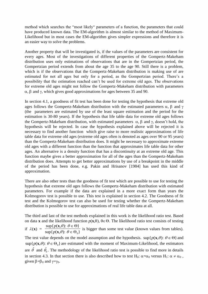
An example where real life table data are used is illustrated in section 3.2. The real

demographic data are collected from Statistical Abstract [1983] and the data are for Swedish

women under the period 1976-1980. A piece of the table in Statistical Abstract, the table used

to have the illustration mentioned above, are shown below.

Age Survivors of 100000 born alive Mean expectation of rested life, years

Men Women Men Women 45 94264 96750 30.23 35.31

46 93928 96555 29.33 34.38

47 93547 96360 28.45 33.45

48 93136 96136 27.57 32.53

49 92721 95891 26.69 31.61

Table 1.1.

Table 1.1. are collected data that shows the numbers of 100000 born alive that are still alive

when they are x years of age (the age are counted when a new year begin) and the number are

arranged in intervals of length one year. The approximation of real demographic data with the

Gompertz-Makeham distribution (the parameters are estimated with help of the least square

estimation with estimated parameters obtained in section 3.2) gives very good results. The

relation between the Gompertz-Makeham distribution and real demographic data for Swedish

women is shown below in Figure 1.1.

30 40 50 60 70 800.55

0.6

0.65

0.7

0.75

0.8

0.85

0.9

0.95

1

age

f(s)

Figure 1.1 the Gompertz-Makeham distribution (with parameters = 5.202*10-3

,

=7.786*10-6

and = 0.1116) - - - - real demographic data.

As you can see of Figure 1.1 the Gompertz-Makeham distribution gives a very good

approximation of real demographic data. This explains why it is of interest to use the

Gompertz-Makeham distribution for different approximations relating to life length theory.

The basic reason for making approximations of real demographic data with use of the

Gompertz-Makeham distribution is that there are many different professions that have great

use of these kind of approximations of life table data. One of the professions that have great

use of the Gompertz-Makeham distribution are insurance companies. The Gompertz-

Makeham distribution would give them better possibilities to determine insurance’s that better

explains the mortality among people for both accidents and natural deaths and it would be

very helpful when the fees of the insurance’s are decided. The Gompertz-Makeham

distribution isn’t only useful for approximating life lengths for human populations. It might

even be of importance to use it in many different biological ways, for example plant biology

has great use of the Gompertz-Makeham distribution. Also life lengths for different crops are

an application where the Gompertz-Makeham distribution can be of importance to use. The

possibility to study life lengths for different crops might even give the possibility to choose a

treatment that in some sense raise the quality of these crops.

2 Properties and characteristics of the Gompertz-Makeham distribution

The Gompertz-Makeham distribution is a distribution that gives very good approximations to

empirical distributions of life length not only for human populations but also for different

biological arts. There will be investigations of some properties of the Gompertz-Makeham

distribution in this section.

The Gompertz-Makeham distribution has the survival function:

F s( ) = exp[-s-e 1s

]. (2.1)

Where s is life time always non-negative ( s 0) and , and are known non-negative

parameters and + > 0 and hence

F s( ) > 0 for s > 0 and F 0( )= 1. (2.2)

How different values of this three parameters influence to the model will be researched. In

general the hazard function of the Gompertz-Makeham distribution often can be used to

express the behaviour of the distribution.

The (cumulative) hazard function of a distribution can be defined by the relation

H(s):= ln(1

F s( )), = (,,), (2.3)

and the intensity hazard function is the derivative of the (cumulative) hazard function

h(s):=dH s)

ds

(. (2.4)

The Gompertz-Makeham distribution has the cumulative hazard function

H(s) = s+e s

1 (2.5)

and the intensity hazard function is

h(s) = +es

. (2.6)

Formulas (2.5) and (2.6) can easily be derived from it’s survival function (2.1) and the

definitions of the hazard functions (2.3) and (2.4). Note that H(s) > 0 if s > 0 due to (2.2).

Another property that can be derived is the probability density function of the Gompertz-

Makeham function

f(s) = dF s)

ds

(=

d(1 - e

ds

-H(s) ) = h(s) e

-H(s) = (+e

s)exp(-(s+

e s

1)). (2.7)

It will be of interest if there exists any points of extremum not at the boundary of the

probability density function of the Gompertz-Makeham distribution. This knowledge is

necessary for the possibility to conclude if the probability density function of the Gompertz-

Makeham distribution is unimodal or not. The probability density function is unimodal if the

derivative is 0 for at most one value of the derivative. The derivative of the probability density

function (2.7) of the Gompertz-Makeham distribution is

df s)

ds

(=

d( h (s)e )

ds

-H(s)

= ( h' ( s) - h2

(s)) e-H(s)

=

= ((es

) - ( +e

s)2) e

-H(s), (2.8)

Because as stated in expression (2.6) the intensity hazard function of the Gompertz-Makeham

distribution is h(s) = + es

and therefore the derivative of it is h' (s) = es

.

Right hand side of equation (2.8) is 0 only when the statements (es

) = ( + es

)2 is true,

because 0 < H(s) < and e-H(s)

> 0. There exists one or two points of extremum only when

(es

) = ( + es

)2 and the values of the life length that gives this equality are positive.

Set z = es

, then (2.8) can be rewritten as

z = ( +z)2 =

2 + 2z + z

2 or

z2 = (-2)z -

2 . The value z can be solved by a second grade equation so the roots are

z1 =

2(1- 1- 4 / )-, and z2 =

2(1+ 1- 4 / )-, and in time scale

s1 =1

ln (

1

(

2(1- 1- 4 / )-)), (2.8)

s2 =1

ln (

1

(

2(1+ 1- 4 / )-)). (2.9)

As earlier defined , and 0. We have s1 s2, otherwise the solution is a natural

logarithm of a negative value, which is a complex value and for that case s1 and s2 will have

complex time. This fact makes sure that the points of extremum occur at non-negative time if

they exist. If s1 is positive (s1 exists) there are two possibilities. Either there exist both a local

minimum and a local maximum of the probability density function or there exists an

inflection point and there doesn’t exist any other point of extremum separated from the

boundary of the function, occurs if s1 = s2. If s1 isn’t positive and s2 is positive then there exist

only a local maximum of the density probability function. If s2 isn’t positive there are no

points of extremum for the probability density function of the Gompertz-Makeham

distribution. The function is unimodal if there are no local maximum not at the boundary of

the function.

Corollary (2.11)

There exists an inflection point of the probability density function of the Gompertz-Makeham

distribution if and only if 4 = and > . ■

Proof of corollary (2.11)

There exists an inflection point for the probability density function if and only if s1 = s2 and

the value of s1 is positive. s1 = s2 if expressions (2.9) and (2.10) are equal expressions. The

expressions are equal if 1-4/ = 0 4 = . Set 4 = and it follows that s1 = s2 ,

s1 = 1

ln(

1

(

2(1- 1- 4 / )-))) =

1

ln(

1

(

4

2

-))=

1

ln(

1

(

2(1+ 1- 4 / )-))) = s2

s1 non-negative implies that ln(1

(2-)) > 0 or (2 -)/ > 1 or > . There exists an

inflection point if and only if 4 = and > . Which was to be proved. ■

Corollary (2.12)

There exist a local minimum not at the boundary of the probability density function of the

Gompertz-Makeham distribution if 4 < , 2(+) < and < (+)2

are true statements. ■

Proof of corollary (2.12)

Local minimum not at the boundary of the probability density function of the Gompertz-

Makeham distribution exists if s1 is positive or 1

ln(

1

(

2(1- 1- 4 / )-)) > 0

1

(

2(1- 1- 4 / )-) > 1

(1- 1- 4 / ) > 2(+) 1- 1- 4 / > 2(+)/

1-2(+)/ > 1- 4 / , no complex solutions allowed

1- 4 / > 0 4 < (2.13)

(if 4 = then there is an inflection point, instead of a local minimum not at the boundary)

1-2(+)/ > 0 or 2(+) < (2.14)

( 1- 4 / )2 < (1 - 2(+)/)

2 if conditions (2.13) and (2.14) are true then

1-4/ < 1+4(+)2

/2 -4(+)/

< (+)2

(2.15)

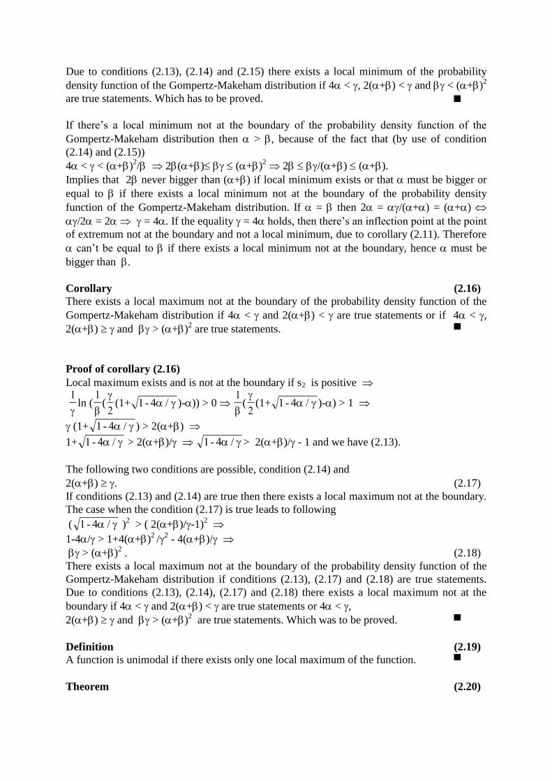
Due to conditions (2.13), (2.14) and (2.15) there exists a local minimum of the probability

density function of the Gompertz-Makeham distribution if 4 < , 2(+) < and < (+)2

are true statements. Which has to be proved. ■

If there’s a local minimum not at the boundary of the probability density function of the

Gompertz-Makeham distribution then > , because of the fact that (by use of condition

(2.14) and (2.15))

4 < < (+)2/ 2(+) (+)

2 2 /(+) (+).

Implies that 2 never bigger than (+) if local minimum exists or that must be bigger or

equal to if there exists a local minimum not at the boundary of the probability density

function of the Gompertz-Makeham distribution. If = then 2 = /(+) = (+)

/2 = 2 = 4. If the equality = 4 holds, then there’s an inflection point at the point

of extremum not at the boundary and not a local minimum, due to corollary (2.11). Therefore

can’t be equal to if there exists a local minimum not at the boundary, hence must be

bigger than .

Corollary (2.16)

There exists a local maximum not at the boundary of the probability density function of the

Gompertz-Makeham distribution if 4 < and 2(+) < are true statements or if 4 < ,

2(+) and > (+)2 are true statements. ▀

Proof of corollary (2.16)

Local maximum exists and is not at the boundary if s2 is positive

1

ln (

1

(

2(1+ 1- 4 / )-)) > 0

1

(

2(1+ 1- 4 / )-) > 1

(1+ 1- 4 / ) > 2(+)

1+ 1- 4 / > 2(+)/ 1- 4 / > 2(+)/ - 1 and we have (2.13).

The following two conditions are possible, condition (2.14) and

2(+) . (2.17)

If conditions (2.13) and (2.14) are true then there exists a local maximum not at the boundary.

The case when the condition (2.17) is true leads to following

( 1- 4 / )2 > ( 2(+)/-1)

2

1-4/ > 1+4(+)2

/2 - 4(+)/

> (+)2 . (2.18)

There exists a local maximum not at the boundary of the probability density function of the

Gompertz-Makeham distribution if conditions (2.13), (2.17) and (2.18) are true statements.

Due to conditions (2.13), (2.14), (2.17) and (2.18) there exists a local maximum not at the

boundary if 4 < and 2(+) < are true statements or 4 < ,

2(+) and > (+)2 are true statements. Which was to be proved. ▀

Definition (2.19)

A function is unimodal if there exists only one local maximum of the function. ▀

Theorem (2.20)

The probability density function of the Gompertz-Makeham distribution function is unimodal

if and only if 4 is a true statement, or if (+)2 and 2(+) are true statements or

if 4 < and > (+)2 are true statements. ▀

Proof of theorem (2.20)

By definition (2.19) the probability density function of the Gompertz-Makeham distribution is

unimodal if the only local maximum that exists of the function is at the boundary or if the only

local maximum of it is not at the boundary of the boundary. The only local maximum is at the

boundary (s=0) of the function when corollary (2.16) isn’t true. If corollary (2.16) isn’t true,

the following statements are correct, 4 or both 2(+) and (+)2 are true

statements.

The only local maximum isn’t at the boundary if there exists a local maximum not at the

boundary and there doesn’t exist a local minimum separated from the boundary of the

function. This is the case when corollary (2.16) is true and corollary (2.12) isn’t true.

Corollary (2.16) is true if 4 < and 2(+) < are true statements or if 4 < , 2(+)

and > (+)2 are true statements and corollary (2.12) isn’t true when 4 and/or 2(+)

and/or (+)2 are true statements. Corollary (2.16) is true and corollary (2.12) isn’t

true only if 4 < , 2(+) and > (+)2 are true statements or if 4 < , 2(+) <

and > (+)2 are true statements, i.e. corollary (2.16) is true and corollary (2.12) isn’t true

when 4 < and > (+)2 are true statements.

The probability density function of the Gompertz-Makeham distribution is unimodal if 4

is a true statement or 2(+) and (+)2 are true statements or if 4 < and >

(+)2 are true statements. Which has been proved. ■

There are four different possibilities of the shape of the probability density function for the

Gompertz-Makeham distribution. The different shapes that are possible are illustrated below

in Figure 2.1- 2.4.

0 2 0 4 0 6 0 8 0 1 0 0 1 2 00

0 . 0 0 5

0 . 0 1

0 . 0 1 5

0 . 0 2

0 . 0 2 5

0 . 0 3

0 . 0 3 5

0 . 0 4

0 . 0 4 5

a g e

f ( s )

F i g u r e 2 . 1

Figure 2.1 shows the function for the values of , and that are estimated in section 4,

namely = 5.44*10-3

, = 7.12*10-6

and = 0.113 and is an example of the probability

density function of the Gompertz-Makeham distribution having a local maximum not at the

boundary of the function.

0 2 40 . 1 2

0 . 1 4

0 . 1 6

0 . 1 8

0 . 2

0 . 2 2

0 . 2 4

0 . 2 6

F i g u r e 2 . 2

2 2 2 . 2 2 . 2

a g e

f ( s )

0 2 40

0 . 1

0 . 2

0 . 3

0 . 4

0 . 5

0 . 6

F i g u r e 2 . 3

0 2 40 . 1 4

0 . 1 6

0 . 1 8

0 . 2

0 . 2 2

0 . 2 4

0 . 2 6

F i g u r e 2 . 4

Figure 2.2 shows an example of the probability density function for the Gompertz-Makeham

distribution having a local maximum both at the boundary and not at the boundary of the

function where the parameter values are = 0.2, = 0.05 and = 0.85. Figure 2.3 shows an

example of the probability density function of the Gompertz-Makeham distribution where the

function has a global maximum at the boundary of the function. The values of the parameters

are = 0.2, = 0.4 and = 0.9. Figure 2.4 shows an example of the probability density

function of the Gompertz-Makeham distribution where the function has a global maximum at

the boundary of the Gompertz-Makeham distribution and an inflection point not at the

boundary of the function. The values of the three parameters are =0.2, = 0.05 and =

0.8.

Another property that is of interest to research are the relationships between the median value

and the mean value of the Gompertz-Makeham distribution. Is the median smaller than the

mean value for known , and for the function or not ?

Notable, the median is the value where F(s) = ½.

F(s) = 1-e-H(s)

= ½ e-H(s)

= ½ H(s) = ln(2) s + e 1s

= ln(2)

s + e 1s

- ln(2) = 0 (2.21)

s can’t be solved explicitly as a expression of , and .

Therefore the only possibility to have a solution of the median is to have a solution with help

of a numerical method. A numerical method that often is used for this kind of approximations

is the Newton-Raphson method. With help of the Newton-Raphson the median value will be

found with good approximation. The median value will be found as the root of function (2.20)

(the root is where the equality of (2.21) holds). The Newton-Raphson is a method that iterates

until an approximation has been found with as many digits as desirable of the median value.

The main problem with the Newton-Raphson method is that a start value must be chosen for

having the possibility to start the iterations that this method is build upon. The start value that

is used can’t be chosen too far away from the root of the function. Otherwise the function

won’t converge to a value and it won’ t give any good solution of the existing problem. To

find a useful start value it’s often necessary to use a different method. This method must have

the possibility to give a value that’s close enough to the searched root, so that the Newton-

Raphson method can be used. The advantage of the method is that the method converges very

fast to the searched root. The Newton-Raphson method is faster than most of the other

methods. That is the justification of the method.

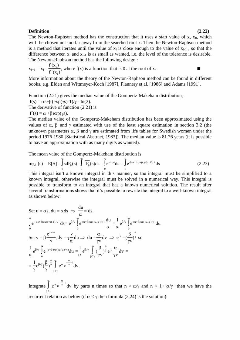
Definition (2.22)

The Newton-Raphson method has the construction that it uses a start value of x, x0, which

will be chosen not too far away from the searched root x. Then the Newton-Raphson method

is a method that iterates until the value of xi is close enough to the value of xi-1 , so that the

difference between xi and xi-1 is as small as wanted, i.e. the level of the tolerance is desirable.

The Newton-Raphson method has the following design :

xi+1 = xi - f (x )

f ' (x )

i

i

, where f(x) is a function that is 0 at the root of x. ■

More information about the theory of the Newton-Raphson method can be found in different

books, e.g. Elden and Wittmeyer-Koch [1987], Flannery et al. [1986] and Adams [1991].

Function (2.21) gives the median value of the Gompertz-Makeham distribution,

f(s) = s+(exp(s)-1)/ - ln(2).

The derivative of function (2.21) is

f´(s) = +exp(s).

The median value of the Gompertz-Makeham distribution has been approximated using the

values of , and estimated with use of the least square estimation in section 3.2 (the

unknown parameters , and are estimated from life tables for Swedish women under the

period 1976-1980 [Statistical Abstract, 1983]). The median value is 81.76 years (it is possible

to have an approximation with as many digits as wanted).

The mean value of the Gompertz-Makeham distribution is

mF,1 (s) = E[S] = sdF s

0

( )= F s)ds

0

( = e ds -H(s)

0

= e ds-( s+ (exp( s)-1) / )

0

(2.23)

This integral isn’t a known integral in this manner, so the integral must be simplified to a

known integral, otherwise the integral must be solved in a numerical way. This integral is

possible to transform to an integral that has a known numerical solution. The result after

several transformations shows that it’s possible to rewrite the integral to a well-known integral

as shown below.

Set u = s, du = ds du

= ds.

e ds-( s+ (exp( s)-1) / )

0

= e/

edu

-(u+ exp( u/ ) / )

0

=1

e/

e du -(u+ exp( u/ ) / )

0

Set v = e u/

,dv =

v

du du =

vdv e

-u =( )

v so

1

e/

e du -(u+ exp( u/ ) / )

0

=1

e/

( )

ve

vdv-v

7

=

= 1

e/

( )

7

1

e v dv-v .

Integrate

7

1

e v dv-v by parts n times so that n > / and n < 1+ / then we have the

recurrent relation as below (if < then formula (2.24) is the solution):

/

e v dv-v1

=

( e

-/( )

-

/

( )

e v dv-v1 1

) = .... = (2.24)

=

(e

-/ ( )

+ (/

)j

i

i 1

n-1

j -

1

1

e

-/ ( )

i

- 1

i - /i 1

n-1

/

( )

e v dv-vn 1

).

mF,1 (s)=1

e/

( )

(e

-/ ( )

+ ( (/

)j

i

i 1

n-1

j -

1

1

e

-/( )

i

)- ( )1

i - /i 1

n-1

/

( )

e v dv-vn 1

)

=

= 1

(1 + ( (

/)

j

i

i 1

n-1

j -

1

1

( )

i )- ( )1

i - /i 1

n-1

e/

( )

(n-/,/)) (2.25)

If < then

mF,1 (s) =1

(1- e

/ (/)

/ (1-/,/)) (2.26)

Where (n-/,/) denotes an incomplete gamma-function. The incomplete gamma-function

has the advantage that it’s a known function that has been evaluated numerical. With help of

tables and different packages for computers (for example ”Mathematica”) it’s possible to have

any well-approximated value of the function for any combinations of , and . By help of

”Mathematica” the mean life time for Swedish women (using life table data for the period

1976-1980) [Statistical abstract, 1983], based on (2.26), is calculated with use of the values of

, and estimated in section 3.2 (The values of the parameters are = 5.44*10-3

, =

7.12*10-6

and = 0.113). The mean life time in this case can be derived from function (2.26),

while < . It’s very likely that formula (2.26) can be used in all cases when mean life time

for human populations are calculated. The mean life time for Swedish women in the given

period is 78.72 years. The table value for the mean life time of Swedish women calculated in

Statistical Abstract [1983] is 78.51, this value is close to the mean value for the Gompertz-

Makeham distribution with estimated parameters. This fact indicates that the mean value for

the Gompertz-Makeham distribution is useful.

The relationship between the median and the mean value is researched with the quotation of

the median and the mean value for different values of , and . The quotation is me

m

F

F,1

and

from (2.21) and (2.25) we can calculate the quotation for given parameters. By use of the

estimated values for , and the quotient, estimated for the case of Swedish women

described above, the quotation is calculated and the quotation is 81.76/78.72 = 1.039. That

means that if the assumption that the life length follows the Gompertz-Makeham distribution

is correct more than half of the Swedish women lives at least a little bit longer than the mean

life length for Swedish women.

The truncated distributions for the median value and even the mean value, with the truncation

at the point t = T can be of some interest to estimate. The estimations can be useful for

different branches, for example for the insurance companies it can be of great use when the

life insurance fee is set for different people.

The truncated distribution of the median value is :

meF (s | t T) =F s + t

F t

( )

( )=

e

e

H(s+t)

-H(t)

= e-(s+t)-(exp((s+t)-1)/)

/e-t-(exp(t)-1)/)

=

= e-(s+exp(t)(exp(s)-1)/)

= ½

s+et (e

s-1)/ - ln(2) = 0. (2.27)

The truncated distribution of the median value can then, as in the case without having a

truncation at t = T (just set T = 0 and it will be exactly the case as without truncation, because

if T = 0 then equation (2.27) will be equal to equation (2.21), i.e. s+e0

(es

-1)/ =

= s+1 (es

-1)/ = s+ (es

-1)/ ), be used and it will give a approximation of the median

value with very good exactness. The approximations of the median value will be done with

use of the Newton-Raphson definition (2.22) as described earlier in this section.

The truncated mean value is:

mF,1 (s | t T) = E[S | t T ] = sdF s

0

( )=F s t

F tds

( )

( )

0

=e

eds

H(s t)

H(t)

0

=

=e

eds

(s t)+ (exp( (s+t))-1) / )

-( t + (exp( t)-1) /

(

0

= e ds-( s+ exp( t)(exp( s) -1) /

0

(2.28)

Set = et,

and e

t are constants so that with use of equation (2.24) and changing with

equation (2.28) will have the same outfit as equation (2.24), but with the difference that will

be changed with in equation (2.28). If the truncation is at T = 0 (no truncation at all), the

mean life time for the rest of the life time is the same as for new-born babies, namely the

equality = e 0

= . The difference between the mean life time left from a truncation at the

age t and the mean life time from day of birth is the constant . The constant is et times

bigger than the constant for mean life time, the constant , used for the calculation of mean

life time from day of birth.

The truncated distribution for the median and the conditional distribution for the mean life

time are for the ages 50, 55, 60,...., 85, 90 as shown in table (2.1) below

From the table below the pattern seems to be that with growing age the mean value will begin

to decrease less than the median value of life time left at the age t. Somewhere between 65

and 70 mean life time starts to be bigger than the median age left.

t meF mF,1 quotient table value of mean life time

left 50 32.49 31.04 1.042 30.69 55 27.70 26.51 1.040 26.22

60 23.03 22.16 1.032 21.88

65 18.55 18.05 1.019 17.73

70 14.38 14.27 0.997 14.11

75 10.65 10.89 0.964 10.39

80 7.50 8.00 0.919 7.52

85 5.02 5.64 0.867 5.30

90 3.21 3.81 0.816 3.65

95 1.98 2.48 0.766 2.35

Table (2.1), the median of the life time left and the mean life time left, at age t. From the table

for Swedish women earlier mentioned in this section[Statistical Abstract, 1983].

3 Programs for simulation and estimation of parameters

In this section of the work there has been written a program to produce simulated values of life time of the

Gompertz-Makeham distribution. This program is explained in section 3.1. A program for the least square

estimation has also been written, the program estimates the unknown parameters in the Gompertz-Makeham

distribution. Explanation of the program can be found in section 3.2. Descriptions of different methods of

estimation can be found in section 3.2, 3.3 and 3.4. The least square estimation is explained in section 3.2. Two

other methods of estimation are also described, namely the method of Maximum-Likelihood in section 3.3 and

the EM(expectation-maximisation)-algorithm in section 3.4.

3.1 Simulation of the Gompertz-Makeham distribution

In order to find a way of determining different properties of the Gompertz-Makeham distribution there often

arises situations where simulation of life times are necessary to do. That’s because of the fact that it can be very

difficult to solve some problems without using simulation and in some cases there aren’t even any known

methods to solve the problems explicitly without help of simulation. There is also the possibility that the

solutions in some cases can be quite complicated to find and the solutions aren’t that much better than the results

obtained by simulation. Therefore it is reasonable to simulate the solution instead of solving the problem

explicitly. When simulation is used it is most often very important that the number of simulations for life times

will be large, otherwise it is possible that too much information will be lost.

The life time will be simulated by splitting the hazard function in two parts. The two parts of the hazard function

are s and (es

-1)/ . Taking , and as known parameters, of course when we have real data , and aren’t

known parameters, to make it possible to simulate life times. The unknown parameters must in some way be

estimated. By splitting the hazard function in two parts there will be two independent life times simulated. The

minimum of this two simulated life times (when the hazard function is split in two parts) is used as the ”real” life

time. The life times obtained are then useful for investigations of different properties. This simulation study gives

possibilities to compare different methods of estimation. For example the expectation and variance of different

estimators such as the estimators for the least square estimate, the method of Maximum-Likelihood (ML) and the

estimator of the method of moments can be compared and conclusions about the best estimator of those are

possible to do.

While the survival function are as stated in (2.1)

= exp[-s- ].

The two parts to be separated are

w1:= exp[-s1 ] and (3.1.1)

w2:= exp[-exp((s2)-1)/]. (3.1.2)

H1(s) = -s and H2(s) = -

From expressions (3.1.1) and (3.1.2), s can be solved explicitly so that s1= and

s2= ln(1- ln(w2)).

A normal explanation of the two different parts of the hazard function is that the first part, with the life length s1,

describes the risk for death in an accidental way and the other part, with the life length s2, describes the risk for

death caused by diseases and other decrements in the healthy state due to the ageing process. This explanation

gives us an reason why the hazard function is split in two parts. Therefore an improvement to categories the faces

of the different parts in the hazard function is possible to do and it is also possible to give a logical explanation

how the deaths are distributed in real life (the percentage of deaths caused by accidents and deaths caused by

decrements in the healthy state). Another advantage of splitting the hazard function in two parts is that this

simulation technique is much faster than the technique without splitting the hazard function. The faster simulation

technique is therefore natural to use while also a logical explanation of the technique exist.

Theorem (3.1.3)

If S = min(S1, S2), where S1 =- and S2 = ln(1- ln(W2)),.then

H(u) = H1 (u) + H2 (u).

S1 and S2 are independent stochastic variables and W1 and W2 are stochastic variables uniformly distributed in

the interval [0,1]. ■

Note: W1 and W2 can be thought of as numbers being produced from a random number generator.

Proof of theorem (3.1.3)

=P(S >u) = P(min (S1 , S2) > u) =P((S1 > u) (S2 > u)) =

(because the fact that if min(S1 , S2) > u then both S1 and S2 must be bigger than u)

= P(S1 >u) P(S2 >u) = F u1( ) F u2 ( ) = eln( F u1 ( )

)+ln( F u2 ( ) )

= e- H1 (u)- H2 (u)

H(u) = H1 (u) + H2 (u) which was to be proved. ■

A program has been written in Pascal for simulation of life times. This program is possible to use for different

applications according to the Gompertz-Makeham distribution. The program uses the equality S = min (Ur ,Vr ).

The program has the following construction :

(1) Fix values of , and are taken, all of them following statement (2.2), i.e. , and are known

non-negative parameters and + > 0 and hence F s( ) > 0 for s > 0.

For having any set of the data it is necessary to have values of , and that are chosen in a

realistic way. For example if the value of is chosen close to 0.2 or bigger, the values of the

Gompertz-Makeham distribution for that values will, if even the value of is chosen

unsatisfactory, tend to be very large and depending on software the computer won’t

have the ability to do all of the calculations that are necessary for a solution.

(2) Set Ur = -ln(W2r)/ and Vr = ln(1-/ln(W2r+1))/. Set Sr = min(Ur, Vr), r = 1,....,n.

Where Ur , Vr and Sr denotes the r:th value of the simulated life time and Wr is a

stochastic uniformly distributed variable in the interval [0,1]. Sr will be the simulated value of

life time. The simulated life times are now available to use for different

applications.

More information about the program for simulations of life time is possible to find in appendix.

3.2 Estimation of the parameters in the Gompertz-Makeham distribution

with use of the least square estimation

The least square estimation is used in this section to make it possible to estimate the unknown parameters in the

Gompertz-Makeham distribution corresponding to ”real” life table data. The least square estimation is a method

of estimation that minimises the sum of all squares between known observations and a given function with

unknown parameters. The combination of the unknown parameters that has the least sum of squares will then be

used as estimated parameters.

In this work a program has been written in the program language Pascal. The program makes it possible to obtain

the least square estimation for the unknown parameters (, and ) of the Gompertz-Makeham distribution. The

structure of the program is described in the appendix of this work with for example the algorithm of the program.

The appendix also contain an example where use of real demographic data has been done. The example makes

use of life table data for Swedish women [Statistical Abstract, 1982] under the period 1976-1980. The program

that has been written for estimating the least square estimator has got the following overall algorithm (the

function that the least square estimation is using is the survival function of the Gompertz-Makeham distribution

with unknown parameters , and ):

(1) Find values of the three unknown parameters that approximately corresponds to the

demographic data that are available, just by testing different values of the unknown

parameters.

(2) Use the values of the unknown parameters that approximately corresponds to real data and use

them, the values are obtained in (1). The values of the parameters will then be tested

for different possibilities of the first digit of necessity of the value of the three

parameters. The combination of the first number for the three parameters will then be used in next

step. Next step will be to test next digit of the parameters and the combination of the

parameters that gives the best estimation will be used in next step and this will continue until

enough digits of the parameters have been calculated.

(3) Repeat (2), but change the ”start” value of the parameters to the value of the parameters that was

obtained in (2) as the best estimator. Stop this procedure when the least square

estimator won’t give more than small enough changes between the two steps. Note, in the program

there will be a comparing procedure that changes the least square estimator and the

parameters of it if the value of the sum of squares are less than the least value that has been

derived earlier.

More about the program is possible to find in the appendix. If the steps in the algorithm is followed it is possible

to have the estimated values of , and with as many correct digits as wanted. The parameters for the example

mentioned above are estimated with help of the program and the values of the estimated parameters are =

5.202*10-3

, = 7.786*10-6

and = 0.1116. Better values of the parameters is possible to have but the values are

good enough for having an acceptable estimation. Figure 1.1 shows the Gompertz-Makeham distribution and real

life table data with estimated parameters and it’s easy to understand that the parameters are useful. The plots of

the two curves are subjoined in the same plot by use of MatLab. The points for real demographic are in this

computer program connected to each other, though the fact that the real demographic data behaves like a discrete

function. The ages for the demographic data are 30, 31,...., 79, 80 years.

3.3 Estimation of the parameters in the Gompertz-Makeham distribution

with use of the method of Maximum-Likelihood

The least square estimation is one of the methods of estimation that can be used to estimate the parameters in the

Gompertz-Makeham distribution. Another frequently used method for estimation is the method of Maximum-

Likelihood.

The method of Maximum-Likelihood was first proposed by Gauss in 1821 and is a method that makes sense

mostly in parametric models. Suppose f(x,) is the density function of x if is true and that is a subset of n

dimensional space. Consider f(x,) as a function of for fixed x. This function is normally called the Likelihood

function with the notation L(,x), where x is thought of as a set of observations. The method of Maximum-

Likelihood consists of finding the values (x) ( =( , ,...., 1 2 k )) which are "most likely" to have produced

known data L( (x), x). It is also possible to have the Maximum-Likelihood estimator without assuming that the

complete data are known. If X=x, the (x) which satisfies

L( (x), x) = f(x, (x)) = max { f(x,) : } is necessary to find.

If such a exists, this value estimates any continuous function q() by q( (x)) . The estimate q( (x)) is called

the Maximum-Likelihood estimation of q(). The method of Maximum-Likelihood is closer described in several

books for example Bickel and Doksum [1977].

The estimation obtained for the Gompertz-Makeham distribution with use of the method of Maximum-Likelihood

is at the point where the derivative, with respect to all parameters in the model is 0, i.e. the point where

f(x, )

i

= 0 for i =1,2,3 and 1 = , 2 = and 3 = .

The survival function of the Gompertz-Makeham distribution is, as stated in (2.1),

F s( ) = exp(-(s+e s

1)). The function can be separated in two parts, F s

'( ) = exp(-s) and F s' '

( ) = exp(-

e s

1)), whose have the probability density functions

f '

(s) = exp(-s) and f ' '

(s) = exp(s)exp(-e s

1)). The probability space of the function are xo = (S1,1,

S2,2....,Sn,n), with Si, i=1,...,n, known observations and i = I(Si = Si

'), most often there is no knowledge of i.

The probability of the i:th outcome is

p0 (si,i) = f '

(si)F s''

i ( ) i +f ' '

(si)F si

'( )(1-i) = i exp(-si)(( exp( s ))i

i1

so the Likelihood function of the Gompertz-Makeham distribution is

L(,x) = i

n

1

(f '

(si)F s''

i ( )i +f ' '

(si)F si

'( )(1-i) =

i

n

1

i exp(-si)(( exp( s ))ii1).

From the expression above the loglikelihood function can easily be derived

l(,si, i) = ln L(,si) = -si+ln(+ e si ) - e s

1.

The Maximum-Likelihood can be solved with 3 non-linear systems, where

l( x)

i

, = 0 for

i =1, 2, 3 and 1 = , 2 = and 3 = .

3.4 Estimation of the parameters in the Gompertz-Makeham distribution

with use of the EM algorithm

Another method that is possible to use for the estimation of parameters of the Gompertz-Makeham distribution is

the EM(expectation-maximisation)-algorithm. The EM-algorithm is almost like the method of Maximum-

Likelihood, but in most cases there will be a simpler way to solve the problems when the EM-algorithm is used

instead of the method of Maximum-Likelihood.

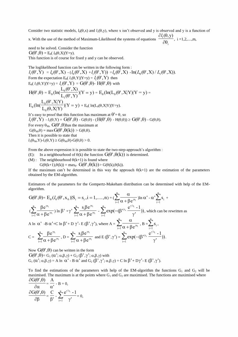
Consider two statistic models, l0(,x) and l1(,y), where x isn’t observed and y is observed and y is a function of

x. With the use of the method of Maximum-Likelihood the systems of equations

l1( y)

i

,, i =1,2,....,m,

need to be solved. Consider the function

G( ' , ) = E( l0(,X)|Y=y).

This function is of course for fixed y and y can be observed.

The loglikelihood function can be written in the following form :

l1( Y ' , ) = l0( X ' , ) - ( l0( X ' , ) + l1( Y ' , )) =l0( X ' , ) -ln( ( ' , ) / ( ' ,L L0 1 X X)).

Form the expectation E( l1(,Y)|Y=y) = l1( Y ' , ) then

E( l1(,Y)|Y=y) = l1( Y ' , ) = G( ' , )- H( ' , ) with

H( ' , ) = EL X)

L Y)Y y

0

1

(ln(

( ' ,

( ' ,)| ) = E L X|Y)|Y = y0 (ln( ( ' , ) =

EL X|Y)

L X|Y)Y y

0

0

(ln(

( ' ,

( ,)| ) + E( ln(L0(,X|Y)|Y=y).

It’s easy to proof that this function has maximum at '= , so

l1( Y ' , ) - l1(,Y) = G( ' , ) - G(,) - (H( ' , ) - H(,)) G( ' , ) - G(,).

For every M, G( ' , )has the maximum at

G(M,) = maxG( k) ' , ( ) > G(,).

Then it is possible to state that

l1(M,Y)-l1(,Y) G(M,)-G(,) > 0.

From the above expression it is possible to state the two-step-approach’s algorithm :

(E): In a neighbourhood of (k) the function G( k) ' , ( ) is determined.

(M) : The neighbourhood (k+1) is found where

G((k+1),(k)) = max‘ G( k) ' , ( )> G((k),(k)).

If the maximum can’t be determined in this way the approach (k+1) are the estimation of the parameters

obtained by the EM-algorithm.

Estimators of the parameters for the Gompertz-Makeham distribution can be determined with help of the EM-

algorithm.

G( ' , )= E x S s ,i 1,....,n0 i i ( ( ' , )|l0 ) = (

e s

i 1

n

i)ln ' - ' si

i=1

n

+

(

e

e

s

si 1

n i

i

) ln ' + ' s e

e

i

s

si 1

n i

i

- exp( ( ''

))

'

is

ie -1s

i 1

n

, which can be rewritten as

A ln ' -B '+C ln '+ D '- E (' , '), where A =

e s

i 1

n

i, B = si

i=1

n

,

C =

e

e

s

si 1

n i

i

, D = s e

e

i

s

si 1

n i

i

and E (' , ') = exp( ( ''

))

'

is

ie -1s

i 1

n

.

Now G( ' , ) can be written in the form

G( ' , )= G1 ('; ,,) + G2 (' , '; ,,) with

G1 ('; ,,) = A ln ' - B ' and G2 (' , '; ,,) = C ln '+ D '- E (' , ').

To find the estimations of the parameters with help of the EM-algorithm the functions G1 and G2 will be

maximised. The maximum is at the points where G1 and G2 are maximised. The functions are maximised where

G( ', )=

A

' - B = 0,

G( ', )=

C

' -

e -1s

i 1

n i

'

'

= 0,

G( ', )= D -' (

s e

'

e -1i

's s

i 1

n i i

'

') = 0.

Set = (k), = (k) and = (k) and with use of the maximisation-step in the algorithm the values of ', ' and ' are set to '= (k+1), ' = (k+1) and ' = (k+1).

The solution will then have the following EM-algorithm

(k+1) = B(k)

A(k),

(k+1) = C k

(e k s

i 1

n

i

( )

)( )

1

11

,

1

1( )k

D(k)

C(k)=

s e

(e

i

(k +1)s

i=1

n

k s

i 1

n

i

i

( ) )1 1

.

For the first two, (k+1) and (k+1), a solution can be decided explicitly from the formulas while (k+1) has to

be solved numerically. Now it is possible to estimate the parameters of the Gompertz-Makeham distribution with

respect to the EM-algorithm. More about the EM-algorithm is possible to find in Cox and Oakes [1984] and

Belyaev and Kahle [1996].

4. Testing of some hypotheses

Of interest it is if the Gompertz-Makeham distribution with estimated parameters (parameters that are mainly

estimated for the ages between 30 and 80) is acceptable even for extreme old ages. Is there a possibility to use the

estimated parameters of the Gompertz-Makeham distribution even for extreme old ages or not? With different

well-known tests it’s possible to test if the estimated parameters of the Gompertz-Makeham distribution are

possible to use even for extreme old ages. Three of the tests that are possible to use are the goodness of fit test,

the Kolmogorov test and the likelihood ratio test. There is a big disadvantage with the Kolmogorov test, namely

that most often there has to be more information about the age than whole years for having the possibility to use

the Kolmogorov test.

The hypothesis that the Gompertz-Makeham distribution with estimated parameters can be tested also for

extreme old ages is tested versus the hypothesis that the estimated parameters can’t be used for these extreme old

ages. If the hypothesis that life table data for extreme old ages follows the Gompertz-Makeham distribution with

estimated parameters is rejected, then those parameters can't be used even for extreme old ages. If that is the case,

the best choice maybe is to use another function to have approximation of extreme old ages. If the Gompertz-

Makeham distribution describes all but the extreme old ages and another function describes the extreme old ages,

there will be a truncated function. The truncated function must have the characteristic of a distribution function,

i.e. 0 < f(si) < 1 and f(s )ii 1

k

1 for i = 1,....,k (it's possible that k is ). Note, two other possibilities are that

instead of a truncated function another function than the Gompertz-Makeham distribution is used for the whole

age interval or the Gompertz-Makeham distribution is used with a more likely set of the estimated parameters.

Another function than the Gompertz-Makeham distribution isn’t of interest in this work while it seems like the

Gompertz-Makeham distribution gives the best description of life table data.

4.1 The Goodness of fit test

One of the methods that are possible to use for the test of such a hypothesis is the goodness of fit test. The

(multinomial) goodness of fit test is a test that makes use of a test statistic called Pearson's 2 . This statistic is

2

2

N(f (s |s ) f (s |s

f (s |s

i j i j

i ji j

k ))

). (4.1)

Where N is the total population size of the researched ages. f(si|sj) is real demographic data for death at the ages

sj, ...., sk-1 and death at ages older than sk-1. sk denotes the probability to die after the age sk-1, given that alive at

age sj (had had j:th birthday). f(si|sj) is the value of the conditional probability density function of the

Gompertz-Makeham distribution at age si given the condition that si sj. Note : i j

k

f(si|sj) = 1. The test

statistic will be compared with 2(k-j-1) for given significance level. If the value is bigger than

2(k-j-1) the test

will reject the hypothesis.

A goodness of fit test has been done as described in formula (4.1) testing that the demographic data explained in

section 3.2 follows the Gompertz-Makeham distribution with estimated parameters. The test is for ages over 95

years and the hypothesis is that ages over 95 years follows the Gompertz-Makeham distribution with the

parameters estimated in section 3.2. Figure 4.1 below shows a plot with both the survival function of the

Gompertz-Makeham distribution (with the parameters estimated by use of the least square estimation in section

3.2) and values of life time from life table data for women [Statistical Abstract, 1983] for ages between 95 and

100.

95 96 97 98 99 1000.1

0.2

0.3

0.4

0.5

0.6

0.7

0.8

0.9

1

Figure 4.1 x - life table data for Swedish women, - the Gompertz-Makeham distribution with parameters

= 0.0005202, = 0.000007786 and = 0.1116.

By the outfit of Figure 4.1 it’s reasonable to assume that life table data for the ages between 95 and 100 doesn’t

follow the Gompertz-Makeham distribution with the estimated parameters This motivates the fact that there is a

need to use different tests to prove this statement. A (multinomial) goodness of fit test for life table data of

Swedish women has been done with help of a program written in MatLab. See appendix for more information

about the structure of the program. The goodness of fit test has been done assuming that the population of the life

table data are of size 4673 women (assuming that the total population of women are 100000, the total population

is definitely much bigger than this) and the values of f(s) are calculated with help of the least square estimation

of the Gompertz-Makeham distribution, with = ( , , )= = (5.202*10-4

, 7.786*10-6

, 0.1116). The ages that

are used in the goodness of fit test is 95, 96, 97, 98, 99 and 100 years. The result of the goodness of fit test is

20.02. This value is compared with the value for the 1 percentage significance level of the 2-distribution . The

value for the 1 percentage level of the 2-distribution is :

0 95

2 1. ( )k j = 0 95

2

. (5) = 15.09.

The hypothesis that life table data for extreme old ages follows the Gompertz-Makeham distribution with the

parameters ( , , ) can be rejected at the 1 percentage level and therefore at all relevant levels. The conclusion

is that the Gompertz-Makeham distribution with estimated parameters can not be used for extreme old ages.

There has also been tested if the ages 90, 91, 92, 93, 94 and 95 years corresponds to this estimated parameters

and the result of the goodness of fit test for those ages is 56.18.

The probability to die at the ages 95, 96, 97, 98, 99 and 100 years, given the condition that still alive at 95

years of age are :

f(d = 95 (die at age 95) |, s 95 (still alive at age 95)) = 0.296, f(d = 96 | s 95) = 0.230, f(d = 97 | s 95) =

0.171, f(d = 98 | s 95) = 0.121, f(d = 99 | s 95) = 0.081 and f(d 100 | s 95) = 0.1025.

4.2 The Kolmogorov test

Another test that is possible to use is the Kolmogorov test. The Kolmogorov test uses a test statistic that needs

more information about the ages (age in days or weeks instead of years) than the goodness of fit test does.

Therefore it is more difficult to use the Kolmogorov test, while ages in life tables most often are in whole years.

If there's life table data in more detailed form than whole years the Kolmogorov test is a good test statistic to use.

If there is no knowledge of the distribution function F, the natural estimate of the probability F(x) is defined by

( )F xn = [number of Xi x]/n.

Since n ( )F xn has a binomial, B(n,p), distribution with p = F(x), ( )F xn is an unbiased estimate of F(x) with

variance F(x)[1-F(x)]/n. The estimate is consistent, ( )F xn P

F(x) and is asymptotically normal for each x. The

curve (.)Fn is itself a distribution function.

If the sample values are X1 = x1,....,Xn = xn and X is a variable with distribution function (.)Fn , then

P[X=xi] = 1

n, for i = 1,....,n.

Fn (.)is called the empirical distribution function of the sample X1,....,Xn

Not only is ( )F xn consistent for each x, but by the Glivenko-Cantelli theorem [Fisz, 1963],

sup | (x n 0

P

F x) - F (x)|0. The Kolmogorov test statistic for testing the hypothesis H0 : F = F0 is defined by Dn

= sup | ( x F x) - F(x)|n

P

0. It's reasonable to reject H0 in favour of H1 : F F0 for large values of Dn.

For large n it’s better to use n Dn , which converges to the so-called Kolmogorov’s distribution K(y). In the

case of real demographic data for Swedish women [Statistical Abstract, 1983] the Kolmogorov test statistic isn’t

a good test statistic to use while the data are not as exactly as wanted. The test will be more useful if life times are

in days instead of years. In that case it will be more close to the continuity assumption that the Kolmogorov

statistic has. It also should be noted that instead of using ”exact” unknown parameters we use the estimators of

the estimators.

4.3 Likelihood ratio test

Another very useful method of testing parametric hypothesis, such as H0: 0 versus H1: 1, is the

likelihood ratio test. The test statistic that is considered for the likelihood ratio test is given by

L(, ):

, ): x

x

x) =

sup{

sup{

p

p

( }

( }

1

0

, where x are known statistical data

Tests that reject H0 for large values of L(x) are called likelihood ratio tests.

The likelihood function L(,x) = p(x, ) can be thought of as a measure of how well explains the given sample

x = (x1,x2,….,xn). So, if sup{p(x, ) : 1} is large compared to sup{p(x, ) : 0}, the observed sample is

better explained by some 1, and conversely.

When the function that is considered is the Gompertz-Makeham distribution, p(x, ) is a continuous function of

and 0 is of smaller dimension than = 0 1 so the that the likelihood ratio test equals the test statistic

(

, ):

, ): x

x

x) =

sup{

sup{

p

p

( }

( }

0

and this statistic is most often not too difficult to compute.

The four basic steps to evaluate the test statistic is

(1) Calculate the Maximum Likelihood estimate of ;

(2) Calculate the Maximum Likelihood estimate 0 of 0;

(3) Form (x) = p(x, )/ p(x, 0).

(4) Find a function h which is strictly increasing on the range of such that h((X)) has a simple form or a

tabled distribution under H0. Since h((X)) is equivalent to (X) the likelihood test with size is specified

with the (1-):th quantile of h((X)) and is possible to find in a table. More about the theory behind the

likelihood ratio test can be found in e.g. Bickel and Doksum [1977].

For example to test if = 0, given = 0 and = 0 versus H1 0, given = 0 and = 0, for the case of the

Gompertz-Makeham distribution, a simple hypothesis is constructed of the form

(

, , , ):

, , , ):

0 0

0 0

ss

s) =

sup{

sup{

p

p

( }

( }

0

= sup{p

p

( , , }

( , ,

s

s

, ):

, )

0 0

0 0 0

.

While sup{p( }s, , , ): 0 0 0 contains of only constants, besides the time observations s, it is possible

to rewrite the function to p( , ,s, ) 0 0 0 . sup{p( }s, , , ): 0 0 0 = p( , ,s, ) 0 0 , where

denotes the Maximum-Likelihood estimate of . The Maximum-Likelihood estimate of the Gompertz-

Makeham distribution is possible to have with help of numerical methods.

If (s) is large the hypothesis H0: = 0 is rejected versus H1: 0. The value of (s) is compared with table

values of the (1-):th quantile of h((S)). Where S is a random variable having the Gompertz-Makeham

distribution. Wished significance level can then be tested.

5 References

Adams, R.A. (1991). Calculus a Complete Course.

Belyaev, Yu.K., Kahle, W. (1996). Methoden der Wahrscheinlichkeitsrechnung und Statistik bei der Analyse von

Zuverlässigkeitsdaten (draf version).

Bickel, P.J., Doksum, K.A. (1977). Mathematical Statistics Basic Ideas and Selected Topics.

Brody S. (1923). The kinetics of senescence. J. Gen. Physiol. 6: 245-257.

Cox, D.R., Oakes, D. (1984). Analysis of Survival Data.

Elden, L., Wittmeyer-Koch, L. (1987). Numerisk Analys - en introduktion.

Failla, G. (1958). The aging process and cancerogenesis. Proc. N. Y. Acad. Sci. 71: 1124-1140.

Fisz, M. (1963). Probability Theory and Mathematical Statistics, p. 391.

Flannery, B.P., Press, W.H., Teukolsky, S.A., Vetterling, W.T. (1986). Numerical Recipes the Art of Scientific

Computing.

Gompertz, B. (1825). On the nature of the function expressive of the law of human mortality and on a new mode

of determining life contingencies. Phil. Trans. Roy. Soc. (London). Ser. A. 115: 513-585.

Lenhoff, H. M. (1959). Migration of C14

labeled cnidoblasts Exptl. Cell Research 17: 570-573.

Pakin, Yu.V., Hrisanov, S.M. (1984). Critical Analysis of the Applicability of the

Gompertz-Makeham Law in Human Populations. Gerontology 30: 8-12.

Sacher, G. (1956). On the statistical nature of mortality with especial reference to chronic radiation. Radiology.

67: 250-257.

Simms, H. S. (1942). The use of a measurable cause of death (hemorrhage) for the evaluation of aging. J. Gen.

Physiol. 26: (2), 169-178.

Statistical Abstracts of Sweden 1982/1983. (1983). Volume 69.

Strehler, B.L. (1960). Fluctuating energy demands as determinants of the death process ( a parsimonious theory

of the Gompertz function). In “The biology of Aging“ (B.L. Strehler et al., eds.), pp. 309-314 Publ. No. 6, Am.

Inst. Biol. Sci., Washington.

Strehler, B.L. (1962).Time, cells, and aging.