1

The global impacts of climate change under pathways that reach 2, 3 and 4oC above pre-industrial levels

October 2015 N.W. Arnell1, S. Brown2, J. Hinkel3, D. Lincke2, B. Lloyd-Hughes1, J.A. Lowe4, R.J. Nicholls2, J.T. Price4 and R.F. Warren4 1Walker Institute, University of Reading

2Tyndall Centre, University of Southampton

3Global Climate Forum, Berlin

3Met Office Hadley Centre

4Tyndall Centre, University of East Anglia

5Global Climate Forum, Berlin

Version 6.1 (12 October 2015)

This work was supported by the Committee on Climate Change

Cite this report as: Arnell, NW, Brown S, Hinkel J, Lincke D, Lloyd-Hughes B, Lowe JA, Nicholls RJ, Price JT and Warren RF (2015) The global impacts of climate change under pathways that reach 2, 3 and 4oC above pre-industrial levels. Report from AVOID2 project to the Committee on Climate Change.

Funded by

2

Summary

This report describes an assessment of the global-scale impacts of climate change under three different potential temperature pathways through the 21st century. These pathways reach peaks of 2oC, 3oC and 4oC above pre-industrial values by 2100. Impacts are represented by indicators covering the water resources, river flooding, coastal flooding, agricultural, environmental and health (heat) sectors, and population and economic growth are assumed to develop along the same ‘middle of the road’ trajectory under all three climate futures.

If global average temperature was to increase by 4oC by 2100, at the end of the century approximately 2 billion people would be exposed to increased water resources stress, an additional 180 million people would be exposed to river flooding each year, and an extra 40,000 people would be flooded per year in coastal floods even after adaptation. If coastal zones do not adapt to sea level rise this figure could increase to up to 36 million per year. More than 8 billion people would be exposed to heatwaves per year. An additional 650 thousand km2 of cropland would be affected by drought, and global average maize productivity would be reduced by around 30%. Nearly 60% of plant species would see a reduction in their climatically-suitable habitat area of more than 50%, along with more than 30% of mammal species. There is, however, a wide range around these numbers, due to uncertainty in how regional rainfall and temperature changes in the future, and the numbers generally represent exposure to impact rather than actual losses because some adaptation will take place (at a cost).

If the increase in global average temperature was to be limited to 2oC by 2100, then these impacts at the end of the century would be reduced – with the proportional effect varying between indicators depending on the shape of the relationship between change in global average temperature and local impact. Only around 10-25% of the impacts on exposure to water resources stress and drought exposure would be reduced, but between 30 and 50% of the impacts on river and coastal flooding would be avoided, and 55-65% and 65-75% of impacts on plant and mammal habitat loss would be avoided respectively. Between 65 and 80% of the reduction in average maize yield would be avoided, but the most dramatic effect would be on exposure to heatwaves, which would be reduced by between 80 and 85%. The proportional difference between the 2oC and 4oC pathways is more robustly estimated than the actual impacts or the absolute impacts avoided. Even a 2oC world increases exposure to climate risks compared to the situation with no climate change, which would need to be addressed through adaptation.

A climate pathway that reaches 3oC by 2100 has approximately half of the effect of the 2oC pathway, but the difference between the two varies between sectors.

Media interest

Estimates of the impacts of climate change under different temperature pathways will potentially be of interest to the media. The approach involves significant caveats, which are explained in the report, so the actual impacts should be taken as indicative.

3

NERC results

Some of the results presented in this report are based on the development of global-scale impact models funded by the NERC QUEST-GSI project.

4

Contents

1. Introduction

2. Overview of methodology

2.1 General approach

2.2 Climate projections

2.3 Socio-economic assumptions

3. Indicators of impact

3.1 Overview of indicators

3.2 Water sector

3.3 River flood risk

3.4 Coastal flood risk

3.5 Agriculture

3.6 Environment

3.7 Health

4. Impacts under different pathways

4.1 Introduction

4.2 Impacts over time

4.3 Geographic variation in risk

4.4 Impacts avoided by limiting climate change

4.5 Impacts incurred if climate policy targets are exceeded

5. Overview of caveats

References

5

1. Introduction

This report presents assessments of the global-scale impacts of climate change under pathways of change in global mean surface temperature reaching 2, 3 and 4oC above pre-industrial levels by 2100, assuming the same socio-economic scenario. Section 2 presents an overview of the methodology and describes the temperature projections and associated climate and sea level rise scenarios. Section 3 describes briefly the impact indicators used, and Section 4 presents narrative descriptions of potential impacts under the three climate pathways. Section 5 concludes by highlighting the most important caveats. The assessment draws largely from data produced by the AVOID1 project (Arnell et al., 2013) and the NERC QUEST-GSI project (Arnell et al., 2014).

2. Overview of methodology

2.1 General approach

The assessment is based on indicators representing impacts on the water, river flooding, coastal flooding, agricultural, environment and health sectors. In each case, impacts are estimated using a spatially-explicit impacts model (typically at a spatial resolution of 0.5o longitude x 0.5o latitude for the terrestrial impacts) run with climate and sea level rise scenarios and the same set of socio-economic assumptions. Impacts are aggregated to the regional and global scale. All the models – as outlined in Section 3 – have been used in previous global-scale assessments.

2.2 Climate projections

Figure 2.1 shows the change in global mean surface temperature, atmospheric CO2 concentration and global average sea level rise under the three climate pathways.

The 4oC pathway is represented by the SRES A1b emissions scenario: more precisely, it is the median estimate of the change in temperature as simulated by a probabilistic version of the MAGICC energy balance model (Lowe et al., 2009), as used in CCC (2008). The probabilistic MAGICC model samples from a range of plausible parameters representing climate sensitivity, ocean diffusivity and the strength of the carbon cycle feedback.

The 2oC pathway is represented by the AVOID1 A1b-2016-5-L emissions scenario, which has emissions peaking in 2016 and declining thereafter at 5% per year. Again, the temperature pathway is the median estimate from the probabilistic MAGICC model. This emissions scenario was used to represent a 2oC pathway in CCC (2008).

The 3oC pathway1 is represented by a temperature trajectory based on an emissions scenario produced as part of the AMPERE project and included in the IPCC AR5 Working Group 3 data base (Clarke et al., 2014). Specifically, the trajectory is based on the

1 Provided by Dr Dan Bernie, Met Office Hadley Centre

6

AMPERE3_RefPol_CEback emissions scenario (Kriegler et al., 2015), and the temperature pathway is again the median estimate from the probabilistic MAGICC model.

Figure 2.1 CO2 concentrations, global mean surface temperature change and global mean sea level rise change (assuming median uncertainty assumptions in the components of sea-level rise) under the climate pathways. See text for explanation of the differences between the sea level scenarios

For each of the three temperature pathways, spatial climate scenarios defining changes in relevant weather variables (mean monthly temperature, precipitation, humidity and net radiation) were constructed by rescaling patterns produced from CMIP3 climate models (Meehl et al., 2007a; Osborn et al., 2015) to match the change in global mean surface temperature. Up to 21 different climate models were used to construct spatial climate scenarios at a spatial resolution of 0.5x0.5o in order to characterise the uncertainty in projected impacts due to uncertainty in changes in climate at a place. Climate scenarios are then constructed by adding the scaled changes to a baseline 1961-1990 climatology (CRU TS3.1: Harris et al., 2014) to produce perturbed 30-year time series.

The CMIP3 climate models were run in the early 2000s, and assessed in the fourth IPCC assessment report in 2007. The CMIP5 intercomparison (Taylor et al., 2012) used the next generation of climate models incorporating refined representations of physical processes, additional complexities and, often, higher spatial resolutions. However, Knutti & Sedlacek (2013) showed that the spatial patterns of change in temperature and precipitation were very consistent between the CMIP3 and CMIP5 ensembles (accounting for differences in forcing scenarios), and that local model spread did not change much between the CMIP3 and CMIP5 ensemble. It can therefore be expected that whilst the use of CMIP5 patterns rather than CMIP3 patterns could give a different indication of the range of potential impacts at a

7

place, the difference in estimated impacts between the two ensembles will be small compared with the range across the CMIP3 ensemble2.

The sea level rise scenarios include both the effects of thermal expansion as simulated by MAGICC and the net contribution from melting glaciers and ice sheets, following the method of Meehl et al. (2007b). For ice caps and glaciers, area-volume scaling was undertaken, and for ice sheets a surface mass balance equation was applied using climate model outputs of ice sheet dynamics from Gregory & Huybrechts (2006). Uncertainty is represented by using the 10th, 50th and 90th percentiles from the uncertainty associated with ice melt and thermal expansion. Note that the trajectory of change in sea level under the 3oC pathway is different to that under the other two pathways because the assumed evolution of forcings before 2000 is different. This means that the estimated 3oC pathway sea level rise impacts are lower than those under the 2oC pathway until the 2080s.

2.3 Socio-economic assumptions

The future impacts of climate change are dependent not only on changes in climate, but also on how the world’s economy and society change. This assessment considers impacts under one socio-economic scenario, which defines change in national population (rural and urban, and by age category) and GDP. The SSP2 scenario (Schweitzer & O’Neill, 2013)3 summarised in Figure 2.2 represents a medium estimate of future population (Samir & Lutz, 2014; 2015) and GDP (Dellink et al., 2015). The figure also shows, for comparison, population and GDP per capita under the other four SSPs. Regional population and GDP per capita are shown in Figure 2.3. The rate of change in GDP per capita through the 21st century varies between regions (the growth by 2050 is slowest in Africa), but by 2100 current regional differences are reduced under SSP2. GDP is here only used in the coastal flood impact indicator (Section 3.4). In this assessment, the national-scale SSP data are downscaled to the 0.5x0.5o resolution.

Figure 2.2 Global population and per capita GDP under the SSP2 socio-economic scenario

2 This has been demonstrated for water resources and river flood indicators (Arnell & Lloyd-Hughes, 2014) 3 Downloaded from: https://secure.iiasa.ac.at/web-apps/ene/SspDb

8

Figure 2.3 Regional population and per capita GDP in 2010, 2050 and 2100 under the SSP2 socio-economic scenario

9

3. Indicators of impact

3.1 Overview of indicators

The global-scale impact indicators are summarised in Table 3.1. The indicators are aggregated to the regional and global scales.

Sector Indicator

Water Numbers of people living in water-stressed watersheds (<1000m3/capita/year)

Numbers of people living in water-stressed watersheds exposed to a change (increase or decrease) in water stress

Average annual number of people exposed to droughts

River floods Average annual flood risk

Average annual number of people exposed to river floods

Coastal floods Expected annual number of people flooded, with different levels of adaptation

Average annual capital cost of coastal flood protection from dike building

Agriculture Area of cropland with change (increase or decrease) in suitability for cropping

Average annual area of cropland exposed to droughts

Productivity of spring wheat, maize and soybean

Environment Area becoming climatically unsuitable for more than 75% of plant/animal species (“areas of concern”)

Proportion of species losing more than 50% of their habitat area due to climate change

Health Average annual population exposed to heatwaves

Average annual population exposed to increased heat stress (with two different thresholds)

Change in labour capacity

Number of frost-days

3.2 Water sector

Impacts of climate change on water resources are characterised by the numbers of people living in water-stressed watersheds, and the numbers of people living in watersheds where average annual river runoff decreases (increased exposure to water resources stress) or

10

increases (decreased exposure to stress) significantly. See Gosling & Arnell (2013) for more detailed results and a discussion on comparisons with other global studies. A water-stressed watershed is defined as having average annual runoff less than 1000 m3/capita/year (Arnell et al., 2011; Gosling & Arnell, 2013), and a ‘significant’ change in runoff is greater than the standard deviation of 30-year average annual runoff, which varies between 5 and 10%. River runoff at the 0.5x0.5o scale is simulated using the MacPDM.09 global hydrological model (Gosling & Arnell, 2011; Arnell & Gosling, 2013).

Drought frequency for each 0.5x0.5o cell is estimated by calculating the 12-month standardised precipitation index (SPI) from the monthly precipitation time series (McKee et al., 1993): it therefore represents precipitation drought, rather than agricultural or water resources drought. A ‘drought’ is defined as a month with an index of less than -1.5, which occurs around 6% of the time. The SPI is first calibrated for each cell from the baseline 1961-1990 precipitation, and then applied with the same calibrated parameters with the perturbed precipitation series and the frequency of months with an index of less than -1.5 calculated. The SPI is currently recommended as the standard indicator for the characterisation of meteorological drought (Hayes et al., 2011). The impacts of drought are represented by the average annual number of people living in grid cells experiencing drought events.

Both of these indicators represent exposure to impact rather than ‘actual’ impact, because they do not incorporate the effects of current or future management interventions and adaptations.

3.3 River flood risk

The impacts of climate change on river flooding are represented by two indicators, both based on flood frequency distributions estimated from the river runoff simulated using MacPDM.09 at the 0.5x0.5o resolution. The first indicator is a representation of average annual flood loss, estimated by combining the grid-cell flood frequency distribution with a generalised loss function, weighting by the numbers of people living in floodplains within the grid cell, and summing over the region and globe (Arnell & Gosling, 2014). The indicator assumes no protection against flooding – but assumes also that there are no losses in events with a return period in the baseline of less than 20 years – so does not directly represent real-world flood losses. It can be interpreted as representing the sum of losses and investment in protection. The floodplain areas are based on the UN PREVIEW GIS data base (preview.grid.unep.ch), and are assumed not to change over time. They were produced by a combination of historical experience and generalised hydraulic modelling, so represent ‘large’ (not precisely defined) floodplains.

The second indicator is the average annual number of people living in major floodplains affected by flood events greater than the baseline 30-year flood. This is estimated from the parameters of the flood frequency distribution as estimated at each site under baseline and future climates. Again, it does not account for flood protection so does not represent the numbers of people actually flooded and is a measure of exposure to impact. This index is similar in principle to that used by Hirabayashi et al. (2013), although calculated in a different way.

11

3.4 Coastal flood risk

Changes in coastal flood risk are calculated using the Dynamic Interactive Vulnerability Assessment (DIVA) model (Vafiedis et al., 2008; Hinkel & Klein, 2009; Hinkel et al., 2013; 2014), which combines changes in sea level with estimates of vertical land movement to determine local sea level rise. For this projection, DIVA model 5.1.1 is used, updating previous results presented in Arnell et al. (2013) and Brown et al. (2013). DIVA incorporates coastal protection (sea dikes), and two assumptions are made in this analysis. ‘Evolving protection’ assumes that protection levels increase as population and wealth increases in the flood-prone areas, but sea level rise due to climate change is not taken into account. ‘Enhanced protection’ assumes that protection levels increase not only as socio-economic conditions change, but also in response to sea level rise experienced so far (although not in anticipation of future sea level rise). The difference between the two can be interpreted as representing the effects of adaptation to climate change. The cost of adaptation is represented by the annual capital costs of dike building (creating new dikes or raising existing dikes) under enhanced protection. Coastal flood risk is characterised by the expected annual number of people flooded. Note that this indicator is slightly different to the river flood indicator because (i) it accounts for assumed levels of protection and (ii) it considers all return period floods.

3.5 Agriculture

The impacts of climate change on agriculture are represented by changes in the suitability of existing cropland for cropping, changes in exposure to drought events, and changes in the productivity of three major crop types. Effects on suitability are based on changes in Ramankutty et al.’s (2002) generalised crop suitability index, which defines suitability based on soil properties, growing degree days and the availability of water to plants. The index is calculated at a spatial resolution of 0.5x0.5o, over the area currently used for crop production (Ramankutty et al. 2008); changes in suitability in areas that are currently not cropped are not considered. The impacts of changes in meteorological drought characteristics are indexed by the average annual area of cropland exposed to severe drought, as defined by an SPI of -1.5 under the baseline climate (section 3.2).

Changes in the productivity of three example crops - spring wheat, maize and soybean (all both irrigated and rain-fed) - are estimated using the GLAM global crop model (Challinor et al., 2004; Osborne et al., 2012), which includes changes in both climate and CO2 concentration. Maize and wheat are the major food staple crops (with rice), and soybean is widely used both for human consumption and for animal feed (it has the sixth highest global production of all staple crops). Three varieties are simulated for each crop for each grid cell. The variety with the highest yield is selected, along with the optimal planting date, both of which can change with climate. In this way, the crop model explicitly incorporates some autonomous adaptation. Regional average yield for each crop is estimated by weighting the GLAM simulations of yield with current cultivated rain-fed and irrigated areas (Portmann et al., 2010). Potential increases in the area which can be cultivated are not considered. Crop productivity projections are based on just five climate models, and are available for the 2oC and 4oC pathways only. The crop productivity projections do not take into account productivity gains due to improved breeding and farming practices, and impacts of climate

12

change are expressed as a percentage change from productivity under the 1961-1990 baseline climate.

3.6 Environment

Impacts on terrestrial ecosystems are characterised by the area two indicators. The first is the area which becomes climatically unsuitable for more than 75% of species assessed (“areas of concern”: Price et al., 2013), and the second is the proportion of species losing more than 50% of their climatically-suitable habitat area due to climate change (Warren et al., 2013). The indicators are calculated separately for plants and animals, and also for amphibia, birds, mammals and reptiles (Price et al., 2013; Warren et al., 2013). The indicators are based on MaxEnt bioclimatic models which predict the probability of species occurrence at the 0.5x0.5o scale from climate and other site data (Warren et al., 2013): models are available for almost 50,000 animal and plant species, most of which have extensive ranges (Warren et al., 2013). The analysis assumes that species can move to new climatically-favourable grid cells, at a realistic dispersal rate informed by paleoecology and historical evidence (Warren et al., 2013), and therefore incorporates adaptation to climate change.

Impacts under the 3oC temperature pathway are estimated by interpolation between impacts calculated under 2.8oC, 4oC and other pathways (Warren et al., 2013), principally to capture the dispersal rates in the species (see Warren et al., 2013 for more detail). The ecosystem indicators were calculated (Warren et al., 2013; Price et al., 2013) from seven climate models.

3.7 Health

The impacts of climate change on health are represented by three indicators relating to the direct effects of high temperatures: both were used in the Royal Society (2014) Resilience to Extreme Weather report, although are implemented differently here. A third indicator represents cold events.

The first indicator describes the change in the regional number of “people-heatwave events”, defined as the average annual number of heatwave events times the number of people affected by each event (the Royal Society report used the numbers of people over 65 rather than total population). A heatwave event occurs if there are more than five consecutive days where the warm season daily minimum temperature exceeds the baseline (1961-1990) mean daily warm season minimum temperature by more than 5oC (Royal Society, 2014). Over time and with no change in climate, the number of “people-heatwave events” will vary with change in population which, as shown in Figure 2.3, differs considerably between regions. In some regions population reduces after the middle of the 21st century, so the exposure reduces.

The second indicator is based on the Wet Bulb Globe Temperature (WBGT), a widely-used measure of environmental heat stress. A value of 25oC is typically taken to be the upper threshold at which heavy labour can be conducted at 100% efficiency (Royal Society, 2014; Dunne et al., 2013), and a value of 32oC represents a threshold for the suspension of any labour (it is often used, for example, to cancel major sporting events: Willett & Sherwood, 2012) . Here, the impact of climate change is characterised by calculating the regional

13

number of ‘population-heat stress events’, defined as the average annual number of days that the WBGT exceeds 25oC or 32oC, multiplied by exposed population. Note that this is different to the heatwave indicator, which is based on the number of events rather than just days. During the 21st century, the number of population-heat stress events changes with both climate change and population.

The third indicator represents change in the capacity for physical labour. Dunne et al. (2013) developed a simple relationship between WBGT and labour capacity, and this relationship is used here to characterise the effects of climate change on labour capacity. As in Dunne et al. (2013), regional and global averages of labour capacity are calculated by weighting each grid cell value by cell population in 20104.

There is no similar system of thresholds that link cold temperatures to human health. Cold spells are therefore represented by the average annual number of frost days, defined as days with a minimum temperature below 0oC. As with labour capacity, regional and global averages are calculated by weighting each grid cell value by cell population in 2010.

The heatwave and frost-day indicators are calculated for each grid cell from daily minimum temperatures. WBGT is calculated from daily average temperature and humidity. Time series of daily temperature and vapour pressure for each grid cell were produced simply by interpolating monthly temperature and humidity (Section 2.2) to produce a smooth annual cycle. WBGT is estimated from temperature and humidity using the approximations used by Dunne et al. (2013).

4 Calculating weights separately for each year using that year’s population has a small effect on the global average, which varies slightly between different population scenarios because they have different distributions of population growth between countries

14

4. Impacts under different pathways

4.1 Introduction

This section summarises the impacts of climate change over time under the three climate pathways. It also provides an overview of the impacts that would be avoided if global average temperature followed a 2oC or 3oC pathway, relative to the 4oC pathway, alongside an overview of the additional impacts that would be incurred if climate followed a 4oC pathway rather than one curbed by climate mitigation policy.

The focus is on the global-scale impacts of climate change; there is, of course, considerable regional diversity in impact and many global-scale impacts are strongly influenced by changes in specific regions.

Data showing global-scale impacts are presented in an accompanying spreadsheet.

4.2 Impacts over time

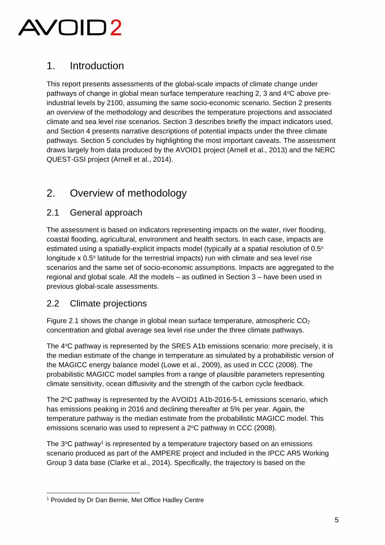
Figure 4.1 shows the trajectory of global-scale impacts over time under the three pathways. For most of the indicators the plots show the median and 10th to 90th percentile ranges across the climate model patterns (assuming all are equally plausible). For the spring wheat, maize and soybean indicators the three values plotted are the minimum, median and maximum across the five climate models, and for the biodiversity indicators the three values are the minimum, median and maximum across seven climate models. For the coastal indicators, the low and high range come from the 10% and 90% ice melt uncertainty and thermal expansion (Section 2.2). Figure 4.2 shows the range in impacts at the global scale by 2100 under the three temperature pathways. The box-whisker plots show the 10th, 25th, 50th, 75th and 90th percentile values across all climate model patterns, assuming each pattern is equally plausible (but only the minimum, median and maximum for the biodiversity, crop productivity and coastal indicators). Most of the indicators are expressed as absolute values, and Figures 4.1 and 4.2 therefore show the indicator in the absence of climate change as a solid black line (Figure 4.1) or a black dot (Figure 4.2).

The median and range is calculated independently for each indicator. No one plausible scenario (for a given temperature pathway) would produce impacts at the upper, median or lower levels across all indicators because of correlations between impacts in different sectors. For example, it is unlikely that one individual climate future would produce both a large increase in exposure to water resources stress and a large increase in river flood risk.

It is important to note that the socio-economic projection used in this analysis assumes global population stabilises after around 2050, with decreases in South and East Asia after then offset by increases in sub-Saharan Africa in particular (see Section 2.3).

Climate change decreases water availability in some water-stressed regions but increases it in others, so the overall net effect is for relatively little change in the total numbers of people living in water-stressed watersheds. However, there are very substantial regional variations in the numbers of people moving into and out of water-stressed conditions, with the vast majority of those apparently becoming less-stressed living in South and East Asia. There is also a wide uncertainty range across the 21 different spatial patterns of change in – particularly – precipitation, especially in South and East Asia.

15

There is a clear signal towards an increase in both the global numbers of people exposed to drought and river flooding events (although not necessarily in the same place), and an increase in average annual flood risk.

A greater proportion of existing cropland (approximately 14 million km2) would see a reduction in suitability for agriculture than would see an improvement: by 2100 almost half of cropland sees a reduction in suitability under the 4oC pathway. There is a clear signal towards an increase in the average annual area of cropland affected by drought. The global average productivity of spring wheat, soybean and maize decreases5, with the pattern over time for maize reflecting the competing effects of changes in temperature and water availability (this reduction in global average productivity might be offset to a certain extent by the prospect of crops being grown in new areas of cropland).

The numbers of people exposed to heatwaves and heat stress increase substantially through the 21st century under the 3oC and 4oC climate pathways – with particularly large increases for high heat stress thresholds - and global average labour capacity declines. The number of frost days also declines.

Increased protection against coastal flooding with increasing wealth (“evolving protection”) means that the numbers of people affected in coastal floods would decline through the 21st century, but this would offset by the effects of sea level rise particularly with the higher temperature pathways6. Adaptation to experienced sea level rise (“enhanced protection”) reduces the number of people affected by coastal floods very significantly, but at cost of approximately $12-$16 billion/year around the middle of the 21st century under the 4oC pathway (compared with annual costs of around $5 billion/year in the absence of climate change).

Finally, under all climate pathways the areas of plant and animal habitats that become climatically unsuitable for more than 75% of species increases through the 21st century with climate change. Under the 4oC pathway, over 50% of plant species are projected to lose more than 50% of their climatically-suitable habitat, alongside a higher proportion of amphibian and a lower proportion of birds, mammals and reptiles.

5 Assuming no secular changes in productivity, due for example to technological or plant breeding developments 6 Note that the 10th percentile impact under the 3oC pathway is slightly lower than that under the 2oC pathway: this is due to the different rate of change in sea level under these two pathways, as shown in Figure 2.1.

16

Figure 4.1 Impacts throught the 21st century under three temperature pathways (4oC red, 3oC blue and 2oC green). The plots show the median impact, along with the 10th and 90th percentile values (minimum and maximum for the crop and ecosystem indicators). Socio-economic scenario SSP2. For some indicators, the black line shows the situation with no climate change.

17

Figure 4.1 (continued)

18

Figure 4.2 Impacts in 2100 century under three temperature pathway.. The plots show the median impact, along with the 10th, 25th, 50th, 75th and 90th percentile values (minimum and maximum for the crop and ecosystem indicators). Socio-economic scenario SSP2. For some indicators, the situation in the absence of climate change is shown by the black dots.

19

Figure 4.2 (continued)

20

4.3 Geographic variation in risk

Figures 4.3 to 4.10 illustrate the impacts for a number of indicators in 2100 under the 4oC pathway, for two illustrative climate models. The maps emphasise the geographic variability in the impact of climate change. Although only two climate model patterns are shown, the comparisons between the two show that the differences in impacts between different climate model scenarios is generally not due to differences in where the impacts occur, but in their magnitude.

The water resources stress maps (Figure 4.3) show the locations of watersheds that would be water-stressed in the absence of climate change (the numbers of people affected, of course, vary considerably between watersheds). The water-stressed watersheds around the Mediterranean and in the Middle East, and in central and southern North America, tend to see an increase in stress, whilst the water-stressed watersheds in South and East Asia see a reduction in stress under one model and an increase with the other (illustrating the strong variability).

Most of the people exposed to an increased frequency of river flooding (Figure 4.4) are in South and East Asia – and a comparison with Figure 4.3 highlights the observation that there is a correlation between impact indicators. The areas with a reduction in water stress in Figure 4.3 are often those with an increase in exposure to flood risk in Figure 4.4.

Figures 4.5 to 4.7 show changes in spring wheat, soybean and maize yields respectively (over currently cropped areas). Spring wheat yields increase in higher latitude areas (northern North America and Russia) primarily due to longer growing seasons, and in parts of East Asia due to greater precipitation. However, elsewhere yields reduce. Soybean yields decrease in most places apart from at the current climate margins. Maize yields decrease virtually everywhere, except in parts of East Asia.

Figures 4.8 and 4.9 show exposure to heat-stress, using WBGT thresholds of 25 oC and 32

oC respectively. By 2100 under the 4oC pathway, heat-stress with the 25oC threshold increases substantially across virtually all of Africa and South America, South and East Asia, the Middle East, the eastern half of the United States, and in southern Europe. With the higher 32oC threshold, the impacts of climate change are largely confined to South Asia.

Figure 4.10 shows the distribution of the number of frost-days, showing very substantial reductions across western and central Europe, much of the eastern United States and parts of north east China.

21

Figure 4.3 Effect of climate change on exposure to water resources stress by 2100, under two climate models: 4oC pathway

Figure 4.4 Effect of climate change on change in river flood risk by 2100, under two climate models: 4oC pathway

Figure 4.5 Effect of climate change on spring wheat yields by 2100, under two climate models: 4oC pathway

22

Figure 4.6 Effect of climate change on soybean yields by 2100, under two climate models: 4oC pathway

Figure 4.7 Effect of climate change on maize yields by 2100, under two climate models: 4oC pathway

23

Figure 4.8 Number of days that WBGT>25: baseline and projections for 2100 under two climate models: 4oC pathway

Figure 4.9 Number of days that WBGT>32: baseline and projections for 2100 under two climate models: 4oC pathway

24

Figure 4.10 Number of frost days: baseline and projections for 2100 under two climate models: 4oC pathway

25

4.4 Impacts avoided by limiting climate change

Limiting the rise in global mean temperature to 2oC would avoid or delay some of the impacts of climate change that would occur if the global mean temperature were to rise to 4oC. Similarly, limiting the rise to 3oC would avoid some of the impacts expected under the 4oC pathway. These avoided impacts could be expressed in absolute terms, but such numbers would be strongly influenced by the assumed socio-economic projection and uncertainty in the pattern of regional impacts due to differences between climate models would result in large absolute ranges. However, expressing avoided impacts in percentage terms reduces – to a large extent – the effect of uncertainty in future socio-economic conditions and reduces – to a lesser extent – the effect of climate model uncertainty.

In principle, limiting climate change can have several different effects on the magnitude of impacts. Most obviously, impacts can be reduced from the level under un-mitigated climate change; at the most extreme, limiting climate change may reduce climate impacts to lower than the levels experienced without climate change. On the other hand, limiting climate change can reduce the beneficial effects of climate change, such as decreases in exposure to water resources stress. Finally, limiting climate change can in some circumstances mean that the beneficial effects of climate change are greater than they would be with un-mitigated climate change. All of these cases can be seen with the indicators considered here.

Figure 4.11 shows the percentage of impacts that would occur in 2100 under the 4oC pathway that would be avoided if temperatures followed a 2oC or 3oC pathway: note that these are not cumulative impacts, but the snapshot of impacts in 2100. The proportion of impacts that are avoided by keeping climate change to 2oC or 3oC varies between sectors and indicators. For some indicators keeping the rise in global mean temperature to 2oC avoids up to 80% of the impacts that would have occurred if temperatures would have risen to 4oC, but for others only avoids around 20% of the impacts. The effect of climate policy on avoided impacts depends essentially on the shape of the damage function relating impact to temperature change: climate policy has relatively little effect if the damage function has a decreasing gradient, but has a large effect if the gradient increases with temperature.

If climate change follows the 4oC pathway, approximately 3000 km2 of cropland would see an improvement in suitability for agriculture (Figure 4.1). However, this total falls slightly through the second half of the 21st century as in some places the beneficial effects of increased temperatures are offset by reduced precipitation, or the beneficial effects of increased precipitation are offset by increased temperatures. If climate change were limited to 3oC or 2oC, then these offsets would be delayed. Under lower rates of climate change the amount of cropland with an improvement in suitability therefore continues to increase through the 21st century (albeit slowly). Limiting climate change therefore increases the beneficial effects of climate change, and this is shown in Figure 4.11 by the negative avoided benefits.

26

Figure 4.11 The percentage of the impacts that would occur in 2100 under the 4oC pathway that would be avoided by a 2 or 3oC pathway. The plots show the 10, 25, 50, 75 and 90th percentiles of avoided impacts (minimum, median and maximum for the crop and ecosystem indicators)

27

Figure 4.11 (continued)

28

4.5 Impacts incurred if climate policy targets are exceeded

The other way of looking at the effect of climate policy on the impacts of climate change is to assess the extra impacts that would occur if the climate policy were not implemented. Figure 4.12 shows the percentage change in impacts in 2100 under the 4oC pathway, compared with the impacts under a 2oC or 3oC pathway (again the impacts are in 2100, not accumulated). As with the avoided impacts, there is considerable variation between the indicators and the extra impacts may be many times those of the impacts which would arise if climate followed the 2oC pathway in particular.

29

Figure 4.12 Percentage change in the impacts that would occur in 2100 if temperatures followed the 4oC pathway, relative to those that would occur under a 2 or 3oC pathway. The plots show the 10, 25, 50, 75 and 90th percentiles for increases in impacts (minimum, median and maximum for the crop and ecosystem indicators)

30

Figure 4.12 (continued)

31

5. Overview of caveats

There are a number of caveats with the assessment, which necessarily mean that the numbers presented are to be regarded as indicative of the potential impacts under the three temperature pathways. The differences between the pathways are more robust than the absolute values under the individual pathways.

The key caveats are:

The climate scenarios representing the changes in climate under the different pathways of change in temperature through the 21st century were produced by pattern-scaling outputs from global climate models. Pattern-scaling assumes that there is a linear relationship between global temperature change and local climate change (which varies from place to place). This assumption may be least reasonable for the pathway with the lowest increases in temperature.

The climate scenarios are based on the CMIP3 generation of climate models, and it is assumed here that all are equally plausible.

The sea level rise projections assume that sea level rise is uniform. Uncertainty in sea level rise projections is here characterised only by uncertainty in the overall magnitude of the rate of total sea-level rise. Due to differential steric changes (e.g. thermosteric or halosteric) and circulation, plus ice melt which can result in gravitational changes due to the shifting ice mass, the magnitude of sea-level rise in different parts of the ocean will vary.

The indicators presented in this report are calculated from one impact model per sector. Different models have the potential to produce different impacts from the same climate scenario (as shown in the ISI-MIP project: Warzsawski et al., 2014), and adding impact model uncertainty would likely increase the range in potential impacts. However, it is not necessarily the case that different impacts models would produce different differences between the three temperature pathways.

The impact indicators mostly represent exposure to impact rather than actual impacts, as they do not take into account either current management interventions or future adaptation (the coastal flood indicator is a notable exception). For most sectors, adaptation is context-specific and conceptually difficult to incorporate credibly into generalised impacts models.

The estimated impacts under all three temperature pathways assume one socio-economic scenario (SSP2). Actual impacts would of course be different under different socio-economic scenarios, and so therefore would be the absolute impacts avoided by reducing the amount of climate change. However, the proportion of impacts avoided by reducing the amount of climate change is much less sensitive to assumed socio-economic scenarios (Arnell et al., 2015).

32

References

Arnell NW. & Gosling SN (2013) The impacts of climate change on river flow regimes at the global scale. Journal of Hydrology 486: 351-364.

Arnell NW & Gosling SN (2014) The impacts of climate change on river flood risk at the global scale. Climatic Change doi:10.1007/s10584-014-1084-5

Arnell NW, van Vuuren DP & Isaac M (2011) The implications of climate policy for the impacts of climate change on global water resources. Global Environmental Change 21(2), 592-603.

Arnell, NW & Lloyd-Hughes B (2014) The global-scale impacts of climate change on water resources and flooding under new climate and socio-economic scenarios. Climatic Change 122: 127-140.

Arnell NW, Lowe, JA, Brown, S, et al. (2013) A global assessment of the effects of climate policy on the impacts of climate change. Nature Climate Change 3, 512-519.

Arnell NW, Brown S, Gosling SN, Gottschalk P, Hinkel J, Huntingford C, Lloyd-Hughes B, Lowe JA, Nicholls RJ, Osborn TJ, Osborne TM, Rose GA, Smith P, Wheeler TR, Zelazowski P (2014) The impacts of climate change across the globe: a multi-sectoral assessment. Climatic Change doi 10.1007/s10584-014-1281-2

Arnell NW, Bernie D, Gambhir A, Lloyd-Hughes B, Lowe JA, Price JT & Warren RF (2015) Interim assessment of the impacts of climate change under specific policy targets. AVOID2 Report B2a to the DECC AVOID2 programme

Brown S, Nicholls RJ, Lowe J, Hinkel J (2013) Spatial variations of sea-level rise and impacts: An application of DIVA. Climatic Change doi:10.1007/s10584-013-0925-y

Committee on Climate Change (2008) Building a low-carbon economy: the UK’s contribution to tackling climate change. Committee on Climate Change, London

Challinor AJ, Wheeler TR, Craufurd PQ, Slingo JM, Grimes DIF (2004) Design and optimisation of a large-area process-based model for annual crops. Agricultural and Forest Meteorology 124:99-120.

Clarke L, Jiang K, Akimoto K, Babiker M, Blanford G, Fisher-Vanden K, Hourcade J-C, Krey V, Kriegler E, Löschel A, McCollum D, Paltsev S, Rose S, Shukla PR, Tavoni M, van der Zwaan B, and van Vuuren DP (2014) Assessing Transformation Pathways. In: Climate Change 2014: Mitigation of Climate Change. Contribution of Working Group III to the Fifth Assessment Report of the Intergovernmental Panel on Climate Change [Edenhofer, O., R. Pichs-Madruga, Y. Sokona, E. Farahani, S. Kadner, K. Seyboth, A. Adler, I. Baum, S. Brunner, P. Eickemeier, B. Kriemann, J. Savolainen, S. Schlömer, C. von Stechow, T. Zwickel and J.C. Minx (eds.)]. Cambridge University Press, Cambridge, United Kingdom and New York, NY, USA.

Dellink RB, Chateau J, Lanzi E & Magne B (2015) Long-term growth projections in shared socioeconomic pathways. Global Environmental Change doi 10.1016/gloenvcha.2015.06.004

Dunne JP, Stouffer RJ & John JG (2013) Reductions in labour capacity from heat stress under climate warming. Nature Climate Change 3, 563-566.

Gosling SN & Arnell NW (2010) Simulating current global river runoff with a global hydrological model: model revisions, validation and sensitivity analysis. Hydrological Processes 25 (7), 1129-1145. doi:10.1002/hyp.7727

Gosling SN & Arnell NW (2013) A global assessment of the impact of climate change on water scarcity. Climatic Change doi:10.1007/s10584-013-0853-x

33

Gregory J & Huybrechts P (2006) Ice-sheet contributions to future sea-level change. Philosophical Transactions of the Royal Society A 364, 1709-1731.

Harris I, Jones PD, Osborn TJ & Lister DH (2014). Updated high-resolution grids of monthly climatic observations - the CRU TS3.10 Dataset. International Journal of Climatology 34(3): 623-642.

Hayes M, Svoboda M, Wall N & Widhalm M (2011) Universal meteorological drought index recommended. Bulletin of the American Meteorological Society 92, 485-488.

Hinkel J, Klein RJT (2009) Integrating knowledge to assess coastal vulnerability to sea-level rise: The development of the DIVA tool. Global Environmental Change 19:384-395.

Hinkel J, Nicholls RJ, Tol RSJ et al. (2013) A global analysis of coastal erosion of beaches due to sea-level rise: An Application of DIVA. Global and Planetary Change 111, 150–158.

Hinkel J, Lincke D, Vafeidis AT et al. (2014) Coastal flood damage and adaptation cost under 21st century sea-level rise. Proceedings of the National Academy of Sciences. doi: 10.1073/pnas. 1222469111.

Hirabayashi Y et al. (2013) Global flood risk under climate change. Nature Climate Change 3, 816-821. doi 10.1038/nclimate1911

Knutti R & Sedlacek J (2013) Robustness and uncertainties in the new CMIP5 climate model projections. Nature Climate Change 3(4): 369-373.

Kriegler E, Riahi K, Bauer N, Schwanitz VJ, Petermann N, Bosetti V, Marcucci A, Otto S, Paroussos L, Rao S, Currás TA, Ashina S, Bollen J, Eom J, Hamdi-Cherif M, Longden T, Kitous A, Méjean A, Sano F, Schaeffer M, Wada K, Capros P, van Vuuren DP, Edenhofer O, (2015) Making or breaking climate targets: The AMPERE study on staged accession scenarios for climate policy Technological Forecasting and Social Change, 90, Part A, 24-44.

Lowe JA, Huntingford C, Raper SCB, Jones CD, Liddicoat SK & Gohar LK (2009). How difficult is it to recover from dangerous levels of global warming? Environmental Research Letters 4(1). 014012 10.1088/1748-9326/4/1/014012

McKee TB, Doesken NJ & Kliest J (1993) The relationship of drought frequency and duration to time scales. in Proceedings of the 8th Conference on Applied Climatology, American Meteorological Society: Boston, MA, Anaheim, CA, pp. 179-184.

Meehl GA et al. (2007a) The WCRP CMIP3 multimodel dataset - A new era in climate change research. Bulletin of the American Meteorological Society 88:1383-+.

Meehl, GA, Stocker TF, Collins WD et al. (2007b) Global climate projections. In Solomon S, Qin D, Manning M et al. (eds) Climate Change 2007: The Physical Science Basis. Contribution of Working Group I to the Fourth Assessment Report of the Intergovernental Panel on Climate Change. Cambridge University Press: Cambridge 433-497.

Osborn TJ, Wallace CJ, Harris IC and Melvin TM (2015) Pattern scaling using ClimGen: monthly-resolution future climate scenarios including changes in the variability of precipitation. Climatic Change. In press

Osborne T, Rose GA & Wheeler TR (2012) Variation in the global-scale impacts of climate change on crop productivity due to climate model uncertainty and adaptation. Agricultural and Forest Meteorology 170: 183-194.

Portmann FT, Siebert S & Doll P (2010) MIRCA2000 – Global monthly irrigated and rainfed crop areas around the year 2000: a new high resolution data set for agricultural and hydrological modelling. Global Biogeochemical Cycles 24: Gb1011 10.1029/2008gb003435

34

Price J, Warren R, and VanDerWal J (2013) The role of mitigation in AVOIDing Potential Climate Change Impacts on Biodiversity. Work stream 2, Report 40 of the AVOID programme (AV/WS2/D1/R40), 71 pp.

Ramankutty N, Foley JA, Norman J, McSweeney K (2002) The global distribution of cultivable lands: current patterns and sensitivity to possible climate change. Global Ecology and Biogeography 11:377-392.

Ramankutty N, Evan AT, Monfreda C, Foley JA (2008) Farming the planet: 1. Geographic distribution of global agricultural lands in the year 2000. Global Biogeochemical Cycles 22. doi: Gb1003 10.1029/2007gb002952

Royal Society (2014) Resilience to Extreme Weather. Royal Society Science Policy Centre Report 02/14. Royal Society, London

Samir KC & Lutz W (2014). Demographic scenarios by age, sex and education corresponding to the SSP narratives. Population and Environment 35(3): 243-260.

Samir KC & Lutz W (2015) The human core of the shared socioeconomic pathways: population scenarios by age, sex and level of education for all countries to 2100. Global Environmental Change doi 10.1016/j.gloenvcha.2014.06.004

Schweitzer VJ & O’Neill BC (2013) Systematic construction of global socio-economic pathways using internally consistent element combinations. Climatic Change doi 10.1007/s10584-013-0908-z

Taylor KE, Stouffer RJ & Meehl GA (2012). An overview of CMIP5 and the experimental design. Bulletin of the American Meteorological Society 93(4): 485-498.

Vafeidis AT, Nicholls RJ, McFadden L, et al. (2008) A new global coastal database for impact and vulnerability analysis to sea-level rise. Journal of Coastal Research, 24,(4), 917-924. doi:10.2112/06-0725.1.

Warren R, VanDerWal J, Price J, Welbergen JA, Atkinson I, Ramirez-Villegas J, Osborn TJ, Jarvis A, Shoo LP, Williams SE and Lowe JA (2013) Quantifying the benefit of early climate change mitigation in avoiding biodiversity loss. Nature Climate Change 3, 678-682.

Warszawski L, Frieler K, Huber V, Piontek F, Serdeczny O & Schewe J (2014). The Inter-Sectoral Impact Model Intercomparison Project (ISI-MIP): Project framework Proceedings of the National Academy of Sciences of the United States of America 111(9): 3228-3232.

Willett KM & Sherwood S (2012) Exceedance of heat index thresholds for 15 regions under a warming climate using the wet-bulb globe temperature. International Journal of Climatology 32: 161-177.