Embed Size (px)
Citation preview

The Global Financial Crisis and its impact on the South African Economy
By
Vongai Madubeko
A dissertation submitted in full fulfillment of the requirements of the degree of Master
of Commerce in Economics.
Department of Economics
Faculty of Management and Commerce
University of Fort Hare
Supervisor: Professor A.Tsegaye
November 2010

ii
Declaration and Copyright
I, the undersigned, Vongai Gwendolene Madubeko, student number 200509125, do hereby declare
that this dissertation is my original work with the exception of quotations and references whose
sources I have acknowledged. I also declare that the work has not been submitted, and will not be
presented at another University for similar or any other degree award.
Vongai Gwendolene Madubeko
30 March 2011

iii
Acknowledgements
My thanks and gratitude goes to Govan Mbeki Research Centre for the financial assistance towards
this research. Opinions expressed and conclusions arrived at, are those of the author and are not
necessarily to be attributed to Fort Hare University or the Research Centre. I would like to express my
sincere gratitude to my supervisor Prof A Tsegaye for his invaluable advice and encouragement and to
Prof S. Ikhide and Mr. U Masunda for their advice and guidance. My gratitude is also importantly
extended to my parents who provided the vital encouragement at the outset, without which the
dissertation would never have been written.

iv
Acronyms and Abbreviations
JSE - Johannesburg Stock exchange
SARB- South African Reserve Bank
GDP -Gross Domestic Product
FCI- Financial Conditions Index
OLS- Ordinary Least Squares
ECT-Error Correction Term
ECM- Error Correction Model
LM- Lagrange Multiplier

v
Abstract
This dissertation investigates the effects of the financial crisis on the South African economy. In order
to do this, an index which describes the financial conditions of the South African economy is
constructed and computed. The index indicates that domestic South African financial conditions have
deteriorated substantially during the period under study and so the study investigates how this has
impacted on the country’s economic growth. A VAR model with South African variables is specified
and used to assess the quantitative effects of the financial crisis on South African real GDP growth.
Results suggest that the South African economy was not significantly affected by the crisis, but
economic growth was slowed down and may still grow substantially slower in the next few years due
to the financial crisis. These results corroborate the theoretical predictions and are also supported by
previous studies.
vi
Table of Contents Declaration and Copyright ........................................................................................................................................ ii
Acknowledgements ................................................................................................................................................. iii
Acronyms and Abbreviations .................................................................................................................................. iv
Abstract .................................................................................................................................................................... v
Chapter one ..............................................................................................................................................................1
Introduction to the Research Study .........................................................................................................................1
1.1 Background .........................................................................................................................................................1
1.2 Statement of the Study ......................................................................................................................................4
1.3 Objectives of the study .......................................................................................................................................5
1.4 Hypotheses .........................................................................................................................................................6
1.5 Justification of the Study ....................................................................................................................................6
1.6 Organization of the study ...................................................................................................................................7
Chapter Two .............................................................................................................................................................8
Background to the Global Financial Crisis ................................................................................................................8
2.1 Introduction ........................................................................................................................................................8
2.2 Overview of financial crises ................................................................................................................................8
2.2.1 Crises in different eras. ................................................................................................................................8
2.2.1.2. Some Recent Financial Crises ............................................................................................................... 10
2.2.3 What makes this financial crisis different?............................................................................................... 18
2.3 Background of the South African Economy ..................................................................................................... 19
2.3.1 Financial Markets and Financial Policy ..................................................................................................... 20
2.3.2 Inflation Rate/ Exchange rate ................................................................................................................... 21
2.3.3 Economic growth ...................................................................................................................................... 22
2.3.4 Developments in the Economy and Transmission of the Crisis into the South African economy ........... 24
2.4 Concluding Remarks ........................................................................................................................................ 31
Chapter Three ........................................................................................................................................................ 33
Literature Review .................................................................................................................................................. 33
3.1 Introduction ..................................................................................................................................................... 33
3.2. Types of financial crises .................................................................................................................................. 33
3.2.1 Definition of a financial crisis.................................................................................................................... 33
3.3 Theoretical Literature ...................................................................................................................................... 35
3.3.1 Theories of Financial Crises ...................................................................................................................... 35

vii
3.3.2 Monetarist Approach ............................................................................................................................... 36
3.3.3 Asymmetric Information: Mishkin’s contribution .................................................................................... 37
3.3.4 Minsky’s financial instability hypothesis .................................................................................................. 39
3.4 Theoretical Framework ................................................................................................................................... 41
3.4.1 The Keynesian Theory of aggregate demand ........................................................................................... 41
3.4.2 The Mundell-Fleming model .................................................................................................................... 42
3.4.3 Linking the Financial markets with the economy ..................................................................................... 45
3.5 Empirical literature .......................................................................................................................................... 46
3.6 General Assessment of the Literature ............................................................................................................. 49
3.7 Conclusion ....................................................................................................................................................... 50
Chapter Four .......................................................................................................................................................... 51
Research Methodology.......................................................................................................................................... 51
4.1 Introduction ..................................................................................................................................................... 51
4.2 Model Specification ......................................................................................................................................... 51
4.3 Data sources and characteristics of variables: ................................................................................................ 53
4.4 An overview of estimation techniques for the study of effect of the Financial Crisis on the Economy ......... 55
4.4.1 Testing for stationarity/ Unit Root testing ............................................................................................... 57
4.4.2 The Dickey Fuller (DF) and the Augmented Dickey Fuller test (ADF) ....................................................... 57
4.4.3 Phillips Perron Tests (PP) .......................................................................................................................... 59
4.4.4 Co integration and error correction modeling ......................................................................................... 59
4.4.5 Johansen technique based on VARS ......................................................................................................... 61
4.4.6 Error correction model (ECM) .................................................................................................................. 64
4.4.7 Advantages of ECM ................................................................................................................................... 65
4.5 Diagnostic Checks ............................................................................................................................................ 66
4.5.1 Autocorrelation test: Lagrange Multiplier (LM) ....................................................................................... 66
4.5.2 White Heteroscedasticity Test ................................................................................................................. 66
4.5.3 Residual Normality Test ............................................................................................................................ 67
4.6 Conclusion ....................................................................................................................................................... 67
Chapter Five ........................................................................................................................................................... 68
Presentation and Analysis of Results ..................................................................................................................... 68
5.1 Introduction ..................................................................................................................................................... 68
5.2. Empirical Findings ........................................................................................................................................... 68
5.2.1 Stationarity results ................................................................................................................................... 68

viii
5.3 The Error Correction Model (ECM) .................................................................................................................. 75
5.4 Conclusion ....................................................................................................................................................... 78
Chapter Six ............................................................................................................................................................. 80
Conclusions, Policy Implications and Recommendations ..................................................................................... 80
6.1 Summary and conclusions ............................................................................................................................... 80
6.2 Recommendations and Policy Implications ..................................................................................................... 81
6.3 Limitations of the study and areas for further research ................................................................................. 83
7.0 References for dissertation ............................................................................................................................. 84
8.0 Appendices ........................................................................................................................................................ A
1
Chapter one
Introduction to the Research Study
1.1 Background
An economy that is healthy and lively needs a financial system that transfers funds to economic
agents with the most productive investment opportunities. A financial crisis interferes with this
process because it can drive the economy away from equilibrium with high output in which financial
markets perform well to one in which output declines sharply because the financial system is unable
to channel funds to those with the best investment opportunities.
The global financial crisis which took a while to develop began showing its effects in the middle of
2007 and into 2008.The financial crisis has spread to developing countries through trade linkages, a
decline in Foreign Direct Investments and remittances, and a large decrease in commodity prices.
Despite the fact that the world economy is still expected to recover in 2010, the downside risk is high.
According Lin (2009), two factors are determinants of the recovery: whether world leaders can rise
above growing popular protectionist pressure, and whether leaders endorse a decisive, coordinated
fiscal stimulus. Coordination will be of great importance, as stimulus enacted by only one or two
countries will be rendered ineffective by international diffusion.
The initial liquidity crisis resulted from the subprime mortgage crisis. According to Akkas A (2009), the
opinion that the global crisis started with the burst of the US housing bubble is not an isolated
phenomenon but is rather linked to the US recession that began in December 2007 following a boom
of November 2007.The crisis was widely predicted by a number of economic experts and other
observers, but it proved impossible to convince responsible parties such as the Board of Governors of
the Federal Reserve of the need for action. One of the first victims outside the US was Northern Rock,
a major British bank. The bank's inability to borrow additional funds to pay off maturing debt
obligations led to a bank run in mid-September 2007. The highly leveraged nature of its business,
unsupportable without fresh infusions of cash, led to its takeover by the British Government and
provided an early indication of the troubles that would soon befall other banks and financial
institutions.

2
Many authors see 2003 as an important threshold in the lead-up to the current financial crisis. This
was the time when the US finally recovered from the IT bubble, growth rose around potential and
Japan nationalized a major bank in response to the earlier financial crisis. The market for securitized
assets grew rapidly especially in the US and investors began demanding more Asian equities.
China’s economy had been booming and it had increased its production capacity. According to Dykes (2009),
the Ned bank group chief economist, China used stimulus policies that included low interest rates and
taxes and experienced large economies of scale therefore driving prices of its products down. These
cheap products from China were exported to Europe and the USA. China had a large current account
surplus which matched the large deficit for Europe and USA. This then resulted in a large buildup in
liquidity and a fall of the cost of money.
South Africa’s economy had also been doing well. The country saw its inflation rate going down to
single digits and had achieved respectable GDP growth and maintained macro stability. According to
Ngwenya, & Zini, (2008), annual GDP growth averaged 5.1% over 2004-07, up from 3.6% over 2000-
03. This was driven by household consumption, private and public fixed investment on the demand
side, financial and business services, construction, and wholesale and retail trade on the supply side.
From then until 2007, when the US housing market began to change, the world financial and
economic environment was favorable. In Akkas’ (2009) view, the US monetary policy enabled people
to borrow at very low cost and this led to excessive lending and as a result the housing bubble
developed. There were a large number of subprime mortgages and the effect of these high-risk loans
had been perceived to be lessened by securitization. However, the strategy appears to have had the
effect of spreading and amplifying it. The securitization schemes eventually failed and the subprime
mortgage crisis thus resulted. Rising interest rates increased the monthly payments on newly-popular
adjustable rate mortgages and property values declined greatly leaving home owners unable to meet
financial commitments and lenders without a means to regain their losses. This led to sharp rise in
foreclosures and an even larger number of homes were dumped into the market. The value of houses

3
in the United States declined because of this excess and the consequence was the developing
financial crisis.
In the run-up to the crisis, low financial volatility, low nominal interest rate and ample liquidity had
increased investors’ appetite for risk. Hedge funds were joined by traditional institutional investors in
the “search for yield” as they expanded their investment in search for wider spreads and higher
returns. Investors did not pay much attention to the risks involved in the complex structured products
they purchased, they trusted the rating agencies to evaluate the risks appropriately.
Akkas (2009) also suggests that the disintegration of the US sub-prime mortgage market and the
problem of the housing boom in other industrialized economies had a ripple effect on the economy of
the whole world. A number of financial products and instruments became so complex that as things
started to untangle, trust in the whole system began failing. The financial system was already
vulnerable because of complicated and highly-leveraged financial contracts and operations and a U.S.
monetary policy that was making the cost of credit negligible therefore encouraging such high levels
of leverage. The extent of this problem has been so severe that some of the world’s largest financial
institutions have collapsed.
As confidence deteriorated banks became unsure of their own liquidity needs and thus stopped
lending to each other, leading to the credit crunch. They began hoarding liquidity worsening the
situation. Initially, central banks provided liquidity to the financial system but the need for liquidity
became persistent and they had to devise new ways of supplying it. Despite central bank’s support,
the crisis deepened and broadened leading to the failure of many financial institutions (such as the
Lehman brothers).
Observers of the meltdown have cast blame widely. According to Ikhome (2008), some observers
highlighted the lack of effective government supervision and described the lending practices of
subprime lenders as greedy. Others have accused mortgage brokers of misleading borrowers into
taking up loans they could not afford even though lenders offered these borrowers programs that
found them acceptable risks, appraisers with inflating housing values, and Wall Street investors with
backing subprime mortgage securities without verifying the strength of the portfolios. Critics have

4
also placed blame on borrowers for over-stating their incomes on loan applications and entering into
loan agreements they could not meet. Some subprime lending practices have also raised concerns
about mortgage discrimination on the basis of race. Ikhome (2008), argues that the effects of the
meltdown spread beyond housing and disrupted global financial markets as investors, mostly
deregulated foreign and domestic hedge funds, were forced to re-evaluate the risks they were taking
and consumers lost the ability to finance further consumer spending, causing increased volatility in
the fixed income, equity, and derivative markets.
The causes of the crisis have become fairly clear, the US housing bubble playing a major role among
other causes. Factors such as the strong liquidity stemming from loose Monetary Policies, financial
innovation, poor regulation and the Chinese surpluses contributed greatly to the global financial crisis.
The US and the UK also had large buildups of debt with the US debt increasing from 90% of household
income to about 130% of household income and UK’s debt to about 175%. What is not so clear,
though, is how the losses incurred could spread to other parts of the global financial system and most
importantly how this affects other economies.
1.2 Statement of the Study
According to Ikhome (2008:2), the argument that Africa stands a reasonable chance of sailing through
the global financial crisis, less bruised than other regions of the world, is based on the fact that some
of the economic weaknesses that have slowed down development of the continent in the past now
appear to serve as a useful shield against the full impact of the crisis. However, while this could be
true of a majority of African economies, it is not true for all of them. Although South Africa, one of the
global South’s emerging markets, is an exception to this rule, its policies such as the exchange
controls, interest rate policy and the National Credit Act insulated it from the direct effects of the
crisis.
Although South Africa’s financial markets have had greater regulation and oversight over the years
that distinguishes them from the financial markets of the more advanced economies of Europe and
North America, it is not completely immune to the effects of the financial crisis. According to Seeraj,
(2008), the country’s debt-driven, consumption-led growth makes it very vulnerable to the credit

5
crunch. In addition to this, South Africa’s financial markets are more closely linked to those of the
industrialized economies of the North and emerging economies than those of other African countries.
Some of the major shareholders in some of the country’s key banks are foreign investors such as
Barclays Bank holdings in ABSA and China’s ICBC recent acquisitions in Standard Bank South Africa.
The factors that drive South Africa’s economic growth have also partly been a result of increased
short-term, foreign portfolio capital flows. Over the years, this made certain the supply of credit and
larger amount of liquidity to the private sector (Seeraj, 2008:13). Together with increased access to
credit, these inflows led to greater speculation in financial and real estate markets and accelerated
consumption growth, which however, did not lead to increased investment. Developing countries
such as South Africa with large trade deficits, and that are dependent on short-term foreign capital
inflows to finance trade deficits, are more vulnerable to the global credit crunch.
When the global financial crisis struck, some of South Africa’s vulnerabilities had already started to
surface. The country battled with high unemployment rate. The agricultural sector was also
underperforming partly because of the floods that were experienced in early 2007.Because consumer
demand was deteriorating globally and also because of the growing energy shortages in the country,
the manufacturing industry suffered immensely, particularly the motor industry. The household debt
as a proportion of GDP was rising fast and the current account deficit started widening. South Africa’s
Political developments especially prior the April elections were also breeding uncertainty and thus
discouraging investment. Because of these vulnerabilities, South African economists and policy
makers have felt the need to assess the effects of the crisis on the country’s real economy in order to
implement policies that would reduce the negative effects.
1.3 Objectives of the study
In the last 80years, the whole world has been affected by the deepest and most serious economic
crisis. Like other countries which are still developing and have a strong integration with the world
economy and depend significantly on its good health, South Africa has been affected by the financial
crisis but this has mainly been second round effects. The result is that growth expectations have had
6
to be sharply revised, downwards. The primary objective of the study is to establish the impact of
financial crisis on the growth of the South African economy.
The specific objectives of this study include:
To critically review the typology of global financial crises.
To establish the extent to which financial crisis has affected South Africa’s macroeconomic
growth.
To make conclusions and policy recommendations based on the findings of the study.
1.4 Hypotheses
The following hypotheses are tested in this study:
An external crisis has a negative impact on South Africa’s economy.
There is a long run relationship between financial markets and the growth of the economy.
1.5 Justification of the Study
Considering the fact that the current financial crisis is more widespread than previous crises, thus
exerting a greater effect on the industrial countries, the perception has arisen that the current crisis
has been stronger in its impact on the affected economies. In this regard, however, recollections of
the hardships endured during previous financial crises may have been dimmed by the passage of
time. The impact of these previous crises has been at least as severe as that of the current crisis. The
crisis has provoked South African economists to look at its causes and the resulting implications for
South Africa. According to Ikhome (2008), when the storm hit, South Africa had been sitting on
relatively strong fundamentals. However, the crisis allowed certain vulnerabilities of the economy to
be exposed. Questions as to what it means for South Africa and its financial sector now that the global
financial system is broken have been raised and thus this study analyses how the crisis that has
impacted on South Africa and the possible solutions that can be undertaken by the government to
lessen the impact.
The analysis will be useful in providing information to both investors wanting to invest in South Africa
and to policy makers in their efforts to improve the growth of the South African economy. Clear-cut
effects of financial crisis on the South African economy are of paramount importance in decision

7
making. Policy makers need information on the precise effects of financial liberalization on developing
economies in order to formulate, evaluate and prescribe policies for the country and therefore the
analysis also strives to identify policy factors that if addressed would prevent such a crisis from
happening again. This study also strives to separate the causal effect of what happened to the
country’s gross domestic product and establish whether the crisis was significant in the reduction of
economic growth.
1.6 Organization of the study
This study is divided into six chapters. The current chapter introduces the problem to be investigated
and focuses primarily on the background of the intended research. It reveals the relevant comparative
historical experiences that led to the financial crisis. Following this introductory chapter is Chapter 2
gives critical review of some of the financial crises that have occurred in the 1990s and also touches
on the various policy responses implemented by countries in an attempt to stabilize the financial
sector. It is intended to shed more light on what constitutes a financial crisis and how the current
financial crisis compares to other financial crises that have been experienced in the past. Chapter 3
reviews both the theoretical and empirical literature pertaining to the financial crisis. Chapter 4 will
present the analytical framework for analyzing the impact of the financial crisis. Following this chapter
is Chapter 5 which will analyze and interpret the results obtained. Chapter 6 will have the conclusions
and recommendations deduced from the results.

8
Chapter Two
Background to the Global Financial Crisis
2.1 Introduction
The financial integration of recent decades has had important benefits for emerging economies, but
has also been associated with increased financial turbulence. South Africa has been no exception,
with local financial markets severely affected by financial crises over the past ten years. These crises
have motivated economists to study the dynamics and underlying causes of financial crises and also
to look at the effects of this turbulence on the economy. This chapter is intended to shed more light
on what constitutes a financial crisis and to also give an overview of the various types of financial
instability experienced over the past decades. The chapter focuses mainly, but not entirely, on events
in developed countries where securities markets as well as banks are important to the financial
system and financial intermediation.
2.2 Overview of financial crises.
2.2.1 Crises in different eras.
The question of how the recent crisis compared with other crises has been touched on and authors
have attempted to address it. According to Allen et al (2007), financial crises have occurred in four
eras i.e. Gold Standard era (1880-1913), The Interwar years (1919-1939), The Bretton Woods Period
(1945-1971) and the recent period (1973-2008). There are several individual financial crises that have
occurred within these periods, the most notable one being the Great Depression of the 1930s. The
different crises will be grouped under past and more recent financial crises and a number of
similarities between the crises and important differences will be highlighted below.
2.2.1.1. Past Financial Crises
i. Pre Great Depression
The most benign period was the Gold Standard Era. During this period, banking crises occurred but
were limited. Currency and twin crises were also limited compared to subsequent periods. The
implication is that globalization does not inevitably lead to crises since the global financial system was
fairly open at this time.
9
The interwar years were the worst with regard to the frequency of crises in the four periods. Given
that this is when the Great Depression occurred, this is not so surprising. Banking crises were
particularly prevalent during this period relative to the other periods.
ii. The Great Depression
The economic damage caused by the current crisis has been said to have worrisome parallels with the
Great Depression of the early 1930s.The Great contraction of 1929-1933 was the worst recession in
the United States of America. Output declined by 34%, prices by 24% and unemployment rose from
4% to 25%. In their monumental “A Monetary History of the United States” (1963), Friedman and
Schwartz argue that the contraction was mostly as a result of a one –third disintegration in the supply
of money which was accelerated by four major banking panics, occurring in succession, starting in
October 1930 and also the failure of the Federal Reserve to follow its mandate and act as a lender of
last resort by using open market purchases to offset these bank failures.
According to Bordo (2009), the many bank failures also resulted in an implosion of financial
intermediation which further contracted the economy In March 1933, the FDR declared a one week
banking holiday during which solvent banks were separated from the insolvent. Only the solvent
banks were to reopen. This is when the contraction ended. In April 1933, large purchases of gold by
the Treasury increased the money supply and changed inflationary expectations from inflationary to
deflationary. This together with the floating of the dollar quickly stimulated recovery.
Allen et al (2007) explains that after the Great Depression, most policymakers were so determined to
prevent such an event from occurring again and so they imposed strict regulations or brought the
banks under state control to prevent them from taking much risk. As a result banking crises were
almost completely eliminated. This period was the Bretton Woods period. Besides the twin crisis in
Brazil in 1962, there were no banking crises at all during the whole period. Frequently, currency crises
did occur but these were mostly because macroeconomic policies were conflicting with the fixed
exchange rates level set in the Bretton Woods system.

10
2.2.1.2. Some Recent Financial Crises
Both emerging and developed countries have become more prone to crises in recent years. There
have been repeated comparisons between the current crisis and past crises such as the Mexican
Crisis, the Asian Crisis and the most frequent one being with the Great Depression which also started
in the USA.
i. The Scandinavian Crises (1985-1986)
According to Allen et al (2007), Norway, Finland and Sweden experienced a typical boom-bust cycle
that led to twin crises. In 1985 and 1986, lending increased by 40 percent in Norway. Prices of asset
hiked whilst consumption and investment also increased significantly. The bursting of the bubble was
mainly due to the collapse in oil prices causing the most severe banking crisis and recession since the
war. In Finland, the massive credit expansion was as a result of an expansionary budget in 1987.
According to Allen et al (2007), housing prices rose by a total of 68 percent in 1987 and 1988. The
central bank also raised interest rates and imposed reserve requirements to moderate credit
expansion. In 1990 and 1991, the economic situation was worsened by a fall in trade with the Soviet
Union. Prices of assets plunged, banks had to be supported by the government and GDP contracted
by 7 percent. In Sweden, a steady credit expansion through the late 1980s resulted in a property
boom. In 1990, credit also tightened and interest rates increased. Several banks experienced severe
problems because of lending that had the foundation of inflated asset values. The government had to
intervene and a recession followed.
ii. Japanese Financial Crisis
According to Allen et al (2007), in the 1980s, the Japanese real estate and stock markets were
affected by a bubble. Japan faced a growing pool of investable funds relative to traditional domestic
investment opportunities, as corporate fixed investment slowed while household saving remained
strong. Financial liberalization throughout the 1980s and the desire to support the United States
dollar in the latter part of the decade led to an expansion in credit. During most of the 1980s, asset
prices rose steadily, eventually reaching very high levels. According to Davis (2003), the introduction
of a new Governor of the Bank of Japan in 1989 who had less interest in supporting the U.S. dollar and
was more concerned with fighting inflation led to the tightening of the monetary policy to counteract

11
the risk of a spill-over of asset price increases into general inflation. In 1990 quantitative restrictions
were also applied to lending for real estate purposes. This led to a sharp increase in interest rates in
early 1990. The bubble burst. Equity and real estate prices fell sharply in Japan from their 1990 peak.
The next few years were marked by defaults and retrenchment in the financial system. Three big
banks and one of the largest four securities firms failed as they faced problems of capital adequacy.
The aftermath of the bubble affected the real economy and growth rates and the consequences were
the banking crisis and recession.
iii. Mexican Crisis (1994)
According to Olivie (2009), in the years leading up to the Mexican crisis, a lot of Latin American
countries initiated economic reforms that attracted the attention of international investors. In the
case of Mexico, the terms for access to certain treaties or organizations (e.g. North American Free
Trade Agreement, OECD and the General Agreement on Tariffs and Trade (GATT)) and domestic
reform process conveyed an economic reform agenda that incorporated domestic economic
deregulation, an opening up in terms of trade and finance and the privatization of public sector
companies in several sectors. International investors, who considered the changes positive, were also
encouraged by low interest rates in the US in the early 1990s.
Foreign financing entered Mexico mainly as bonds. Even though foreign direct investment and shares
on the stock market also brought in money, for the most part, this came from privatization and was
insignificant compared from debt. According to Olivie (2009), debt contracts and titles were also
denominated in foreign currencies. This substantial entry of capital transformed into a credit boom
financing domestic consumption and imports, in addition to the speculative bubbles that emerged in
the real estate sector and the stock market. And since these transactions were denominated in
Mexican pesos, excessive foreign debt and a rise in internal credit directed at high-risk activities
meant that there was a currency imbalance between assets and liabilities.
During the course of 1994, other complications compounded the situation. Some of these were of
economic and others of a political nature. With reference to the economy, one complication that
stands out most is the rise in interest rates in the US market. Moderate levels of interest rates were at

12
least somewhat responsible for capital entry into Mexico in the early 1990s. According to Olivie
(2009), a lower differential in interest rates resulted in a lesser lure of Mexican debt. To make things
worse, a series of events left Mexico engulfed in political instability.
The stock markets began to fall with the eruption of the Chiapas rebellion. Olivie (2009) also discusses
how international investors’ expectations as to profitability and risk intrinsic to the Mexican economy
started to alter. Even though stock indices randomly continued to fall for the remaining months of the
year, Mexican interest rates began to rise as foreign currency reserves declined. By year end, with
exhausted currency reserves, the Mexican authorities had deserted the semi-fixed exchange rate
system, accelerating the collapse of the Mexican peso. Just then, the crisis spread to the rest of Latin
America, resulting in the so called Tequila effect.
iv. The Russian Crisis and Long Term Capital Management (LTCM)
The Long Term Capital Management (LTCM) fund was quite successful during the first two years and
earned very high eturns for its investors until in 1997 when returns declined. By this time, LTCM had
about $7 billion under management and thus decided to return about $2.7 billion to investors as they
were not able to earn high returns with so much money under management. In 1998, Russia devalued
its currency and defaulted on about 281 billion roubles of government debt resulting in a global crisis
with extreme volatility in many financial markets. Flight to quality caused prices to move in
unexpected directions and many of the convergence trades that LTCM had made started to lose
money and lost a lot of capital. According to Davis (2003), eventually, the Federal Reserve Bank of
New York coordinated a rescue whereby the banks that had lent significant amounts to LTCM would
put $3.5 million for 90 percent of the equity of the fund and take over the management of the
portfolio. The reason behind this was to avoid the likelihood of a global meltdown in asset markets
and the systemic crisis that would follow.
v. Asian Crisis (1997)
Up until 1997, Asian countries such as Singapore, Hong Kong, Taiwan (the Dragons) and Thailand
Indonesia and Malaysia (the Tigers) experienced great economic performance. Their economies grew
at sustained high rates for a very long time. According to Allen et al (2007), after sustained pressure,

13
the Thai Central bank stopped defending the Thai Baht and consequently it fell 14% in the onshore
markets and 19% in the offshore markets marking of the start of the Asian financial crisis.
The Philippine peso and the Malaysian ringitt were next currencies to come under pressure. The
Philippine central bank tried to defend the peso by raising interest rates, but it however lost $1.5
billion of foreign reserves and consequently let the peso float, resulting in the currency falling by 11.5
percent. The Central bank of Malaysian also defended the ringitt before letting it float and so did the
Indonesian central bank.
Singapore decided against defending its currency and by the end of September 1997, it had
depreciated by 8 %. Taiwan also stopped defending their currency and let it depreciate but it was not
affected much. According to Allen et al (2007), Hong Kong's exchange rate, which was pegged to the
dollar, was affected severely but however, it was able to maintain the peg. The South Korean won
appreciated against the other South East Asian currencies in the beginning but as time went by and
things got more intense it lost 25 percent of its value. By the end of the crisis in December 1997, the
dollar had appreciated against the Malaysian, Philippine, Thai, South Korean, and Indonesian
currencies by 52, 52, 78, 107, and 151 percent respectively.
Real effects of the crisis were persistent and continued to be felt within the region even though the
turmoil in the currency markets was over by the end of 1997. Output of many industrial and
commercial firms fell sharply and a lot of financial institutions went bankrupt. The crisis was quite
severe and extremely painful for the economies involved.
vi. The Argentina Crisis of 2001-2002
In the 1980s, Argentina's economy did poorly. It suffered through an extended period of economic
instability including the Latin American debt crisis and hyperinflation and had a number of inflationary
episodes and crises. In 1991, it introduced a currency board that pegged the Argentinean peso at a
one-to-one exchange rate with the dollar and limited the printing of pesos only to an amount
necessary to purchase dollars in the foreign exchange market. This ushered in a period of low inflation
and the country enjoyed strong economic growth in the early 90s. Despite these favourable

14
developments, a number of weaknesses developed during this period. Following Mexico’s December
1994 peso devaluation, capital flowed out of emerging markets and Argentina’s GDP declined by
2.8%. In 1997, a number of events occurred, including the crisis in Asia. The financial crisis moved to
Russia and then Brazil. Argentina entered prolonged recession in third quarter and unemployment
began to rise. According to Davis (2003), the public debt the government had accumulated limited the
amount of fiscal stimulation that the government could undertake. Also the currency board meant
that monetary policy could not be used to stimulate the economy. The recession continued to
deepen. At the end of 2001, it began to become clearer that Argentina's situation was not
sustainable. The government tried to alter the way that the currency board operated as a means of
rectifying the situation. Exporters were subject to an exchange rate that was subsidized and importers
paid a tax. The situation in the country worsened. There was a run on the private sector deposits
followed by looting of supermarkets. The government imposed bank withdrawal limitations of 250
pesos per week. According to Davis (2003), this resulted in protests and rioting spread to major cities.
In December 2001, the economy collapsed. Industrial production fell 18 percent year-on-year.
Imports fell by 50 percent and construction fell 36 percent. In January 2002, a new currency system
was introduced by the fifth president which included allowing the peso to float. It soon fell to 1.8
pesos to the dollar. On the whole, the crisis was devastating. Real GDP fell by about 11 percent in
2002 and inflation in April 2002 went to a high of 10 per cent a month.
Common Elements of Current Crisis with the Asian and Mexican Crises
The Asian and Latin American crises of the late 90s have a lot in common with the current global
crisis, although there are also some big differences. It is clear that the three regions all had domestic
economic problems before their respective crises began. A common problem that materializes in all
three regions is the weakness of the system of financial regulation and oversight. With Mexico and
Asia, this may have been the result of financial reforms that were undertaken too fast and/or in a
disorderly fashion.
According to Allen et al (2007), when the asian crisis occurred, the South Korean economy
deteriorated even more in earlier periods in some of its macroeconomic variables without slipping
into a financial crisis. With regards to the Mexican crisis, studies that have been done attribute the

15
rise in interest rates in the US and domestic political instability as the factors that contributed to its
occurrence. In the case of the US, the country has been posting twin deficits for decades. Since the
1990s the US has had a constant current account deficit which it has financed through a debt which
the rest of the world economy has been willing to supply. This was partly because the US dollar is an
international reserve currency.
Parallels of the current crisis with Great depression
Although there has been success in controlling the damage caused by the current crisis, the risks
involved should not be taken too lightly. According to Helbling (2009), the weakening in financial
conditions from balance sheet contraction, asset fire sales, and increased demand for liquid assets
has been more rapid than during the Great Depression and at least as strong, if not stronger. This can
be seen in the diagram below. The current crisis peaked faster than the great depression.
Helbling (2009) also explains that feedback effects on the solvency of financial intermediaries from
deteriorating economic activity have started to materialize. What turned the recession of 1929-30
into the Great Depression was the surfacing of adverse feedback loops between real and financial
sector adjustment in the absence of an offsetting policy. Evidently, policy actions to stop asset price
deflation, avoid debt deflation, reinstate confidence in the financial sector and support a global
recovery need to be maintained.
Figure 2.1 below describes financial factors in the USA. (Baa corporate bond spread months after the
business cycle peak)

16
Figure 2.1: Financial factors in the USA
(Time in Months)
Source: Helbling (2009:23)
Comparisons of the current financial crisis and the great depression have been done by several
authors. The distinction has been between the setting, initial conditions, transmission, and policy
responses.
Helbling (2009) suggests that in both the Great Depression and the current crisis, the US economy was
the centre of the financial contraction. This characteristic differentiates these episodes from the any
of the financial crises that have occurred in the past few decades. A global impact has thus been all
but certain from the onset because of the weight of the US economy and its financial system.
In both episodes rapid credit expansion and financial innovation that led to high leverage paved way
for the crisis. According to Helbling (2009), however, the 2004-07 boom was global whilst the 1920s
credit boom was mainly concentrated in the US. A financial shock to the US economy now has a
greater and more immediate effect on global financial systems because of higher levels of real and
financial integration than during the interwar period. These greater financial vulnerabilities must be
balanced against weaker global economic conditions in 1929. Helbling (2009) also suggests that to a
lesser extent, consumer prices in major economies had already stagnated or started declining before

17
the US recession started. Slowing activity in the economy thus led to deflation almost immediately.
On the contrary, inflation which was above target in mid-2008 has provided an initial cushion in the
current crisis. Key attributes in the financial sector transmission in both episodes were liquidity and
funding problems. At the root of both crises were concerns about the net worth and solvency of
financial intermediaries, although the specific mechanics differed given the financial system’s
evolution.
According to Helbling (2009), in the Great Depression, the problems were as a result of the erosion of
the deposit base of US banks in the absence of deposit insurance. In four waves of bank runs, about
one-third of all US banks failed between 1930 and 1933. The scene for bank runs in countries in
Europe was set by the failure of the Austrian bank Creditanstalt, in 1931. However, in the recent
global financial crisis, deposit insurance has provided some sort of reassurance and has to a greater
extent prevented bank runs by retail depositors. Instead, financial intermediaries have experienced
funding problems relying on wholesale funding, mostly those issuing or holding US mortgage-related
securities whose value was affected negatively by increasing mortgage defaults. Because of increased
cross-border linkages, the problems have immediately reached other nations. On the contrary, during
the Great Depression, the spillovers were more gradual. Rising capital flows to the US and money
supply contraction in the source countries were responsible for the transmission of the US funding
problems.
There has been a strong, swift recourse to macroeconomic and financial sector policy support in the
current crisis unlike in the Great Depression, when countercyclical policy responses were practically
absent. Central banks in the major currency areas have intervened massively to provide financial
systems with liquidity and lowered policy interest rates. Exceptional discretionary fiscal stimulus will
support aggregate demand this year.
According to Bordo (2009), the current crisis which has led to a recession was not caused by a classic
banking panic because the Federal Deposit Insurance Corporation (FDIC) successfully removed the
incentives for depositors to stage runs on their banks. However, the causes were in fact losses in
wealth that were related to the stock market crash that led to even greater wealth losses, contracted

18
consumer spending and investment and collapse of housing prices. Nevertheless a banking crisis is
still a key element of present problems because the interbank lending market dried up, many banks
became insolvent and lending is constrained. Helbling (2009) also explains that in addition to this, the
failure of the subprime mortgage market led to the collapse of the derivatives markets, and because
of the run by creditors on the uninsured investment banks, to the collapse of the shadow banking
system. A major credit crunch also resulted and this is evident in the large hikes in quality spreads and
the paralysis of some credit markets. This also resulted in a serious recession which in turn has
intensified banking system and the financial sector problems. A similarity between the current
recession and the Great depression is that both crises were driven by shocks to the banking and
financial sector, but the orders of magnitude are much less now than then i.e. five quarters into the
recession, real GDP reached about 6% below trend. At the same stage in the Great depression, it was
12% below trend and at its trough in 1933 it was 30% below trend.
2.2.3 What makes this financial crisis different?
The financial crisis that broke out in the US in 2007 and spread to the rest of the world’s wealthy and
developing economies over the course of 2008 caught analysts, governments and private-sector
forces utterly by surprise. Credit crises in the past tended to be confined to the commercial banking
and direct lending sectors. With the growth of the securitization market, investment banking firms
became big players in the mortgage market, as well. This allowed the risk to spread far and wide,
making this crisis that started with subprime lending in the United States both a bank and nonbank, as
well as a global, problem.
Many economists have offered numerous analyses as to the causes of the crisis and have also
debated over the best ways to respond to it. There have therefore been repeated comparisons
between the current global crisis with other crises. One of the most frequent ones is the comparison
with the Great Depression in 1929, which also started in the US. The consequences for the real
economy are compared with those of World War II, and the work that the G-20 countries embarked
on in November 2008 is compared with the process that led to the Bretton Woods accords of 1944.

19
According to Samuelson (2009), each financial crisis, however, has a resemblance to other crises and
passes through similar phases. Nevertheless, each crisis also has its own distinctive characteristics.
Three features distinguish the current economic crisis: Firstly, the proximate origins of the crisis were
in the United States: despite of the amount of blame for the crisis placed on US macroeconomic
policies and on financial regulatory policies, it still remains a fact that the United States led the way
into the crisis. Secondly, if the leading economy in the world, whose currency and financial
institutions are at the foundation of the global financial system, stops performing efficiently, it should
not be surprising that the resulting crisis is global. In this crisis, the citizens and authorities of a
country can run, but they cannot hide. Thirdly, it is quite common for a crisis to begin in the financial
sector, spread to the real economy, cycle back to further deteriorate the financial sector, and in so
doing further aggravate the conditions in the real economy.
According to Samuelson (2009), the analysis of the economic and financial situation was more
complicated in the current crisis. During the greater part of 2008, global growth appeared to be
holding up in general, and inflation, mainly in commodity prices, was still rising. Policymakers were
sluggish in learning that they were dealing with two severe crises on a global scale i.e.,in the financial
system and in the real economy. Numerical evidence about dual crises in the traditional industrial
countries on average reflects that financial decline led to real economy slump. Improvements in the
real economy lead the financial upturns, except for equity prices.
2.3 Background of the South African Economy
South Africa is the economic powerhouse of Africa, leading the continent in industrial output and
mineral production and generating a large proportion of Africa's electricity. The country has abundant
natural resources, well-developed financial, legal, communications, energy and transport sectors, a
stock exchange ranked among the top 20 in the world, and a modern infrastructure supporting
efficient distribution of goods throughout the southern African region.
South Africa has experienced strong economic growth since the ending of Apartheid in the early
1990s. A profound restructuring of the economy has borne fruit in the form of macro-economic
stability, booming exports and improved productivity in both capital and labor.

20
2.3.1 Financial Markets and Financial Policy
South Africa has a sophisticated financial structure with the JSE securities exchange, a large and active
stock exchange that ranks 20th in the world in terms of total market capitalization as of March 2009.
At the end of May 2009, the JSE’s market capitalization amounted to USD614 billion (R4.9 trillion) and
market turnover to USD300 billion (R3.1 trillion) for the 2008 calendar year. The liquidity ratio
increased from 35.5 in 2005 to 41.4 in February 2009.
South Africa has a well-regulated banking sector. The Basel II capital framework was implemented in
January 2008. The SARB started to publish benchmark overnight interbank rates in 2001 and in March
2007, introduced the improved South African Benchmark Overnight Rate on deposits (Sabor).The
South African Reserve Bank (SARB) performs all central banking functions. The SARB is independent
and operates in much the same way as Western central banks, influencing interest rates and
controlling liquidity through its interest rates on funds provided to private sector banks.
According to Mboweni (2009:1-3), in 2009, monetary policy was faced with new challenges. For the
first time since the introduction of the inflation-targeting framework in 2000, monetary policy had to
be implemented in the context of a domestic recession and against the backdrop of the severe and
synchronized downturn in the world economy. At the same time, inflation remained well above the
upper end of the inflation target range and, despite the downside pressures; targeted inflation was
only moderating at a very slow rate.
Even though inflation was still outside the target range, monetary policy was still eased and the MPC
continued to apply monetary policy within a flexible inflation-targeting framework, cognisant of the
economic downturn. Nevertheless, price stability remains the ultimate objective of monetary policy
and the Reserve Bank remains committed to achieving the target over a reasonable time frame.
The South African Government has also taken steps to gradually reduce remaining foreign exchange
controls, which apply only to South African residents. According to Faure (2007), private citizens are
now allowed a one-time investment of up to R2 million in offshore accounts. Since 2001, South
African companies may invest up to R750 million in Africa and R500 million elsewhere. Smaller South

21
Africa Companies can also move up to 50 Million Rand without SARB approval, allowing for swifter
expansion to overseas markets.
2.3.2 Inflation Rate/ Exchange rate
The monetary authorities have tried to keep the country’s inflation rate under control. From 2004
through 2006 consumer inflation came in at under 5% before global prices pressed it up to 6.5% in
2007. In 1994 it stood at 9.8%. Figure 2.2 below shows South Africa’s inflation rate from just before
independence (1993) to 2007.
Figure 2.2: South Africa’s inflation rate (CPIX)
(inflation)
(Time in years)
Source: Statistics South Africa (1997)
According to Mboweni (2009:1-3), inflation clocked in at 6.1% year on year in September, driven
primarily by food price increases – but the rate of decrease is clearly slowing down. Currently, South
Africa’s year-on-year inflation rate stands at 3.70 percent. In 2008, the South African Reserve Bank
(SARB) took steps to compress price pressures. The SARB is allowing the currency to adjust rather
than targeting a specific value for the exchange rate. The Rand plunged almost 30% against the US$ in
2008, and in the early stages of 2009, before regaining lost ground through Q3.

22
Figure 2.3 below shows the country’s inflation rate from January 2008 to July 2010.
Source: Trading Economics.com; Statistics South Africa (2010)
2.3.3 Economic growth
According to an article by SADC bankers (2009:2), South Africa's economy has been in an upward
phase of the business cycle since September 1999, the longest period of economic expansion in the
country's recorded history. As shown in figure 4 below, South Africa's real GDP rose by 3.7% in 2002,
3.1% in 2003, 4.9% in 2004, 5% in 2005, 5.4% in 2006, the highest since 1981 and 5.1% in 2007. In the
fourth quarter of 2007, South Africa recorded its 33rd quarter of uninterrupted expansion in real GDP
since September 1999.
South Africa's economy has been completely fixed since the inception of democratic government in
the country in 1994. Bold macroeconomic reforms have boosted competitiveness, growing the
economy, creating jobs and opening South Africa up to world markets. Over the years these policies
have built up a rock-solid macroeconomic structure. Taxes have been cut, tariffs dropped, the fiscal
deficit reined in, inflation curbed and exchange controls relaxed.

23
Figure 2.4: Growth of GDP in South Africa
(GDP Growth)
(Time in years)
Source: Statistics South Africa (1997)
SADC bankers (2009:2-3) also noted that economic growth and prudent fiscal management have seen
South Africa's budget deficit drop dramatically, from 5.1% of GDP in 1993/94 to 0.5% in 2005/06 - the
second-lowest fiscal deficit in the country's history after the 0.1% reached during the gold boom in
1980. 2006/07 saw the country posting its first ever budget surplus of 0.3%.
According to the World Bank, South Africa Gross Domestic Product (GDP) contracted 2.10% over the
last 4 quarters. In Q1/09 output posted an annualized 6.4% q/q contraction, followed by a 3% q/q
decline in Q2/09. Currently, the South Africa Gross Domestic Product has a proportion of 0.45% of the
world economy or is worth 277 billion dollars. According to Trading Economics (2009), South Africa
has a two-tiered economy; one challenging other developed countries and the other with only the
most basic infrastructure. It is therefore a productive and industrialized economy that displays many
characteristics associated with developing countries, including a division of labor between formal and
informal sectors and an uneven distribution of wealth and income. The primary sector, based on
manufacturing, services, mining, and agriculture, is well developed.
The figure below shows the country’s GDP growth rate from January 2006 to July 2009.It is evident
from the diagram that since the start of the crisis, the growth of the economy has since deteriorated.

24
Figure 2.5: SA GDP growth rate in percentages against time in months
Time
Source: Trading Economics, Global economics Research.2009
2.3.4 Developments in the Economy and Transmission of the Crisis into the South African economy
According to Kershoff (2009:5), the financial crisis was transmitted into the economy mainly through
the financial markets, tightening of bank lending standards and trade linkages. The section below
provides an analysis of the main developments in the South African economy including the financial
system and the real sector. Developments in these sectors have a significant bearing on the stability
of the domestic financial system.
2.3.4.1 Financial Markets
The spread of South African bonds widened at the height of the financial market crisis, but have
narrowed in the meantime. Kershoff (2009:5) also explains that during the global crisis, risk aversion
rose. As shown in figure 2.6 below, foreign portfolio investment flows to emerging countries, such as
South Africa, reversed.

25
Figure 2.6
Time in years
Source: SARB Quarterly Bulletin, Sep. 2009, p. 42
Figure 2.7: Rand exchange rate
Source: SARB Financial Stability Review, Mar 2009, p. 31
Figure 2.7 above shows that after dropping sharply in September 2008, the rand exchange rate
recovered and returned to pre-crisis levels by May 2009.

26
According to SARB Financial Stability Review of March 2009, in the third quarter of 2008 the ratio of
equity market capitalization to GDP dropped substantially even though it was still high. As shown in
Table 2.1 below, an additional drop was experienced in the fourth quarter and this was in line with
developments in the global equity markets. In the third and fourth quarters, no major changes were
recorded with regard to the ratio of broad money supply to GDP and the ratio of private-sector credit
to GDP, and in part this reflected relatively tight credit conditions together with still relatively high
lending rates. Bank intermediation also remained relatively constant.
Table 2.1: Selected indicators of financial-sector development
Source: SARB, Financial Stability Review (2009)
2.3.4.2 Banking Sector
South African banks have been largely protected against the direct effects of the global financial crisis.
According to SARB (2009:8), domestic banks did not invest as heavily in high-risk securities or complex
instruments. They maintained mostly a traditional and relatively conservative banking model,
sustained relatively high lending standards, enjoyed high profitability for a number of years and
maintained high capital levels. Banks also had low levels of foreign funding and limited activity outside
the African continent. For this reason, no banking crisis occurred in South Africa in contrast to many
other countries.

27
As shown in figure 9 below, the liquidity requirements of banks did not surge. According to SARB
(2009:40), the interbank market also continued to operate normally. The South African Reserve Bank
did not have to provide emergency liquidity that many countries had to provide for their financial
institutions. The spread between the policy and market interest rate also did not widen in South
Africa as in many other countries.
Figure 9.Liquidity requirement
Source: SARB Quarterly Bulletin, Sep. 2009, p. 40
2.3.4.3 Confidence in the financial Sector
As measured by the Ernst & Young Financial Services Index, in the fourth quarter of 2008, confidence
in the financial sector dropped to its lowest level since the time the index was first used. According to
SARB (2009:10), the drop, which stemmed from the worsening level of confidence in the areas of
investment banking and specialized finance, was mainly attributed to the impact of the global liquidity
crisis. The level of confidence of investment managers also reduced. Unstable global capital markets
and a weak investment banking environment put a downward pressure on the volumes of business
and this also affected fee income negatively. Investment income also dropped due to the poor
performance of the equity markets.
After dropping significantly in the third quarter of 2008, the retail banking confidence level rose in the
fourth quarter of the same year. However, it was still low compared to previously recorded levels.

28
Although interest income declined due to the decline in credit extension growth on the back of
lending standards, the increase was recorded.
Table 2.2: Financial Services index and its components
Source: SARB, Financial Stability Review (2009)
According to SARB (2009:8-9), falling income and rising expenditure resulted in a contraction in net
profit of retail banks. The confidence level of life insurers was supported by rising premium income,
although this is expected to slow due to adjustments made following a new commission payment
method with effect from January 2009.
2.3.4.4 Bond, equity and currency markets
In the second half of 2008 domestic government bond yields declined, reflecting signs of a deepening
global recession, an easing in inflationary pressure, interest rate cuts and continued weakening of the
equity markets. According to SARB (2009), since January 2009, the yield on the short-dated R153
bond has declined further as a result of the appreciation of the rand, moderation in domestic inflation
and expectations of further interest rate cuts following a cumulative 250 basis point cut since
December 2008. The upward trend in longer-term bond yields since December 2008 can be attributed
to the depreciation of the rand, which resulted in speculation about a possible rating downgrade and
less demand for assets that were perceived as being riskier, as the global economic slowdown
deepened. As the global financial crisis intensified and started to dampen economic growth in the
second half of 2008, the domestic equity market continued its downward trend. According to SARB
(2009), accelerated deleveraging, failures and near-failures of large financial institutions in the
industrial countries, coupled with the weakening of global economic fundamentals, have resulted in
falling asset prices and difficult financial conditions. As concerns over the risk of a global recession

29
gathered momentum and economic growth in EMEs slowed, more pronounced declines in financial
asset values and increases in volatility ensued.
2.3.4.5 Tightening of bank lending standards
Before the onset of the crisis, banks in South Africa had already started tightening credit standards.
These standards stemmed from the new national credit act (NCA) implemented in 2007, the change
to Basel 2 accounting standards and capital requirements in 2008 and rising non-performing loans.
However, in reaction to what happened to banks overseas during the global crisis, South African
banks tightened credit standards even further. According to Kershoff (2009:9), this set a violent circle
in motion. The cut in credit provision intensified the decline in house prices, slowdown in consumer
spending and cut back in fixed and inventory investment. These developments, in turn, sped up
business closures and retrenchments, which led to a further tightening of credit standards.
2.3.4.6 International trade
International trade plunged during the global crisis. South African exports of goods (see figure 11
below) and services fell sharply as a result. According to Kershoff (2009:8-9), South Africa was hit
really hard by the drop in the international demand for vehicles and non-food commodities (industrial
raw materials) mainly because these items dominate the country’s exports.

30
Figure 11: South African exports of goods and services
Time in years
Source: SARB Quarterly Bulletin, Mar. 2009, p. 24
2.3.4.7 Real Economic activity
The overall level of activity in the real economy dropped in the fourth quarter of 2008. Annual
declines were recorded in building plans passed, new vehicle and passenger car sales, and electricity
generated. According to SARB (2009:12), utilization of production capacity also dropped from 85 per
cent in September 2008 to 83 per cent in December. Relatively higher lending rates, together with an
uncertain outlook following developments in the global financial markets, may have contributed to
the decline in real economic activity. The impact of the global economic slowdown on real economic
activity in South Africa is also evident in the retrenchments and business closures particularly in
mining and manufacturing. In the motor industry, for example, the drop in domestic and especially
export demand and the resulting production cuts are a reflection of a sales slump in the rest of the
world.

31
Below is a table showing selected indicators for real economic activity for 2007 and 2008.
Table 2.3: Selected indicators for real economic activity
Source: SARB, Financial Stability Review (2009:12)
2.4 Concluding Remarks
The current financial crisis is more global than any other period of financial turmoil in the past six
decades. The extent and harshness of the crisis reflects the union of several factors, some of which
are common to previous crises and others are new. As in previous times of financial turmoil, the pre-
crisis period was characterized by surging asset prices that proved unsustainable, a prolonged credit
expansion leading to accumulation of debt, the emergence of new types of financial instruments and
the inability of regulators to keep up.
As a result of the global financial turmoil and the slowdown in economic activity, South Africa is
evidently experiencing pressure. Corporations have been affected directly through higher financing
costs, as well as indirectly through the impact of the turmoil on their customers and, hence, their
order books. Exports are under pressure due to the decline in world trade, and the risk of more job
losses in some industries, wage pressures and the costs of production remain high.
Even though financial crisis may be similar with previous crises in some characteristics, the effects of
the current crisis have been the worst ever experienced since the great depression and therefore it
remains significantly different. On previous occasions, whenever the financial system came to the

32
verge of a collapse, the authorities got their act together and prevented it from going over the brink.
This time the system actually broke down and what had been a mainly financial phenomenon
transformed into a calamity that affected the entire economy.

33
Chapter Three
Literature Review
3.1 Introduction
This chapter reviews both the theoretical and empirical literature found on the issue being studied,
that is, the financial crisis and its effects on the economy. Many economists clearly failed to predict
the effects of the US financial crisis on the global economy. Only a few economists were anywhere
near explaining how this crisis would affect different countries. Empirical literature is developed
through taking note of the theoretical strides made to date in explaining how the effects of the
financial crisis in the financial market can be transmitted to the real economy variables.
3.2. Types of financial crises
3.2.1 Definition of a financial crisis
Because it is not easy to determine a common and uniform definition of financial crisis, there is a
huge collection of literature on financial crises based on historical case studies as well as current
economic conditions written by economists. Within this literature there are also numerous
“conclusions”, drawn and some of them are quite contradictory and thereby inconclusive.
Davis (2003) defines a financial crisis as a major collapse of the financial system, entailing inability to
provide payment services or to allocate credit to productive investment opportunities. It is also an
interruption to financial markets that disrupts the market’s capacity to allocate capital and therefore
financial intermediation and investment come to a halt (Portes 1998). According to Nurul (2009:13),
each financial crisis is distinctive in its nature, form, causes and effects, nevertheless a comprehensive
theory can be used to explain the financial crisis. Financial crises are very diverse in terms of timing,
the source of monetary expansion and the object of speculation depending on the time and location.
According to Zavala (2001) (as cited by Nurul (2009:14)), financial crisis are divided into two major
parts; Currency crisis and Banking crisis. He defined Banking crisis as crises that occur when a financial
system becomes illiquid or insolvent. They mainly constitute bank runs, closures, mergers, takeovers,
or large-scale assistant by the government to a group of banks or banking systems, should the crisis
turn out to be systematic. A recent approach to financial crisis is by Mishkin who defines it as, “….a
34
disruption to financial markets in which adverse selection and moral hazard problems become much
worse, so that financial markets are unable to efficiently channel funds to those who have the most
productive investment opportunities”.
Not all financial crises have the same characteristics i.e. financial crises do not recur in an identical
manner, both because institutional composition differ across countries and over time, and because
individuals learn to some limited extent from such problems. According to Davis (2003:5), they can
differ in the manner in which they affect the economy and also in their causes. Over the years, three
principal types of financial instability have been identified and these may be intertwined in any
particular episode.
Davis (2003:5) describes the most common type of financial crisis as that which is centred on bank
failures. This follows a loan or trading losses, examples include the recent global financial crisis, the
banking crisis in Japan and the Asian crisis, just to mention a few. These bank failures tend to result in
a credit crunch, i.e. a contraction of credit supply to the non-financial sector, causing a wider
economic disruption. Within these banking crises, a distinction can be made between those restricted
to domestic financial system and those linked to cross border bank lending and indebtedness in
foreign currencies.
A second type financial crisis mentioned by Davis (2003) entails severe market price volatility
following a shift in expectations. This crisis is unique in that it tends to involve institutional investors
as principals, and is focused primarily on the negative effects of quick price changes, for other
financial institutions, which result from institutions imitating one another's strategies. Whilst volatile
prices may not have systemic implications, these may, however, materialize when these price
movements threaten institutions that have taken leveraged positions on the current levels of asset
prices. An example to note is the Stock Market Crash of 1987. The Asian crisis had elements of this
pattern where aggressive exchange rate movements aided in the set off of banking crises due to
foreign currency exposures of banks and non banks.

35
Davis (2003) also discusses a third type of financial crisis which is similar to the second one. This type
entails a prolonged crumpling of market liquidity and issuance. Like the second type, it also involves
institutional herding, with the only difference largely having to do with whether markets are
sufficiently resilient, and whether market maker structures are robust enough. Such crises also are
inclined to affect debt and derivatives markets rather than equity or foreign exchange. Risks involved
are severe not only for those holding positions in the market but also for those relying on the market
for debt finance or liquidity and these are mainly banks. Past crises of this type were of typically
specific and distinctive markets and these characteristically relied on a narrow investor base, market
maker structure and/or issuer base (e.g. US junk bonds, international floating rate notes). An example
of such a crisis was the collapse of the Russian liquidity market and issuance in 1998 but however, the
events that followed this were much more severe. This was because liquidity failure was threatened
in markets such as the US swaps, securities repurchase, commercial paper, corporate and Treasury
bond market. A major historical precedent was the Penn Central Bankruptcy and its resulting effect on
the US commercial paper market. In these examples, liquidity was threatened in core markets and as
a result, the US authorities had to take a decisive action.
3.3 Theoretical Literature
This section presents the main theories on financial crisis in order to provide a general knowledge on
the subject at hand and to facilitate further analyzing the current financial crisis from a South African
perspective. By looking into the different views and approaches for financial crises, the section also
briefly discusses what the theoretical literature offers as explanation of financial crises. The
theoretical models also guided the choices of the financial and economic indicators used in the
analysis.
3.3.1 Theories of Financial Crises
To understand the relationship between the current crisis and the different crises that occurred in the
past, a conceptual framework to analyse financial crises is needed. According to Allen et al (2007), the
difference between the majority view concerning the cause of crises in the 1930s and the view of
many today is quite remarkable. In the 1930s, the problem was the market and the solution was
government intervention through regulation or direct ownership of banks. Many now argue that

36
conflicting government macroeconomic policies or moral hazard in the financial system caused by
government guarantees is the major cause of the recent crises. The opinion now is that government is
the cause of crises and not the solution and market forces are now the solution.
3.3.2 Monetarist Approach
This approached explains that financial crises are impacted by bank failures on the economy through
the decrease in the supply of money. The crises have a tendency of often being the consequence of
policy miscalculations by monetary authorities generating “regime shifts” that unlike the business
cycle are impossible to allow for in advance in risk-pricing.
According to Nurul (2009:15), banking panics have been identified as a sign of financial crisis by
monetarists. Friedman and Schwartz (1963) pointed out that out of the six main contractions in the
US over 1867-1960, four were mainly caused by major banking or monetary disturbances. This was
due to the public’s loss of confidence in the Central Bank`s abilities to convert deposits into currency.
Confidence on the Central bank deteriorates when a significant institution fails in the market, and that
aids in the development of the crisis. In addition, Friedman and Schwartz’s (1963) view is that the
banking panics were a major source of reduction in the money supply which led to a severe
contraction in the aggregate economic activity.
Schwartz (1987) explains that financial instability is usually caused by inflation which is highly related
with the interest rate as well as money supply and a rise in inflation leads to a rise in interest rate.
This creates problems for the Central Bank particularly if the bank is engaged in fixed rate investment
project or if the Central Bank lends in a fixed rate, even this instable price level may lead to
insolvencies of the bank.
According to Nurul (2009:15), monetarists do not see a necessary link between business cycle and
crisis and they do not rule out asset price bubble. In monetarist view ‘financial crisis` is mainly a shift
to money that leads to widespread run on banks. In particular, banking crises occur when financial
systems become illiquid. This type of financial crisis refers to bank runs, closures, mergers, takeovers,

37
or large scale assistant by the government to a group of banks or to the banking systems, should the
crisis turn out to be systemic.
3.3.3 Asymmetric Information: Mishkin’s contribution
Numerous researches have been done on asymmetric information problem and how it is related to
financial crisis. In simple terms, asymmetric information problem implies the unavailability of
information among the entities in the financial market. According to Nurul (2009:18), in the financial
market, asymmetric information problem might exist in the financial contract between the two most
important entities, that is, the lender and borrower. The borrower has better information than lender
about his return on project and the risk associated with that project. It follows that lender has either
to increase the interest rate which eliminates some high quality borrower or he may choose credit
rationing rather than raise interest rates, in order to avoid adverse selection.
Mishkin (1992) (as cited by Nurul (2009:18)), by providing an analysis of asymmetric information, gave
a framework for how disturbances in financial markets can cause a downturn in the economy. He
defined a financial crisis as; “….. a disruption to financial markets in which adverse selection and moral
hazard become much worse, so that financial markets are unable to efficiently channel funds to those
who have the most productive investment opportunities”.
Asymmetric information and agency costs are aspects of a debt contract which create market failures
of moral hazard and adverse selection and aid in explaining the nature of financial instability, for
example, the tightening of credit as a result of rising interest rates and falling asset prices fall or, as
mentioned by Allen & Gale (1999), the tendency of lenders to make high risk loans due to the shifting
of risk linked to agency problems.
As defined by Mishkin (1992:2), asymmetric information refers to the phenomenon in which one
player has more information than other stakeholders in the financial market. Transactions, that take
place in financial markets, are therefore exposed to asymmetric information, leading to problems
with adverse selection and moral hazard.

38
According to Mishkin (1992:4), adverse selection in financial markets occurs when the likely
borrowers, who the potential to produce undesirable outcomes, are the ones who are likely to be
chosen. Since adverse selection makes it more possible that loans be made to bad credit risks, lenders
may decide against making any loans, even though there are good credit risks in the marketplace.
Mishkin (1992:5) defines moral hazard as that which occurs in financial markets after a loan has been
extended; the lender is subjected to the hazard when the borrower might engage in activities that are
not favourable to the lenders. These activities increase the probability of default. If the borrower
invests in high risk projects, he may do well if the project succeeds, but the lender bears the risk of
losing out if the project fails. Moral hazard and the conflict of interest between the two can result in
lenders deciding not to make loans, and lead to suboptimal levels of lending and investments.
……………………………………………………………………………………………………………………….
Source: Adopted from Mishkin (1992 p.123)
Increase in
interest
rates
Stock
market
decline
Increase in
uncertainty
Adverse selection and moral hazard problems worsen
Decline in aggregate economic activity
Bank panic
Adverse selection and moral hazard problems worsen
Decline in aggregate economic activity
Price level
decline
Adverse selection and moral hazard problems worsen
Decline in aggregate economic activity

39
As shown in the diagram above, Mishkin (1992) (as cited by Binaku (2009:11-12)) identified five key
factors in the economy, which can result into considerable worsening of the adverse selection and
moral hazard in financial markets. This, in turn, can lead to a financial crisis.
These key factors are: 1.) increases in interest rates, 2) stock market declines, 3) increases in
uncertainty 4) bank panics and 5.) Unanticipated declines in the aggregate price level. Increase in
uncertainty, or an increase in interest rates and the stock market crash increased the severity of
adverse selection problems in the credit market, while the decline in net worth of stemming from
stock market crash increased in moral hazard which help lead to a crisis eventually.
3.3.4 Minsky’s financial instability hypothesis
This hypothesis proposes that financial crises follow a credit cycle with an initial positive shock
aggravating rising debt, mispricing of risk by lenders and an asset bubble, which is then burst by a
negative shock, leading to a banking crisis. Patterns like these are perceived as a normal feature of the
business cycle. This is similar to what happened in the recent crisis that developed in the US.
As economic theory, the financial instability hypothesis is an interpretation of the substance of
Keynes's "General Theory" in viewing the capital system as innately unstable because of the instability
of aggregate investments. The theoretical argument of the financial instability hypothesis starts from
the characterization of the economy as a capitalist economy with expensive capital assets and a
complex, sophisticated financial system. Minsky (1992:3-5), identifies the economic problem
following Keynes as the "capital development of the economy.” The focus is on an accumulating
capitalist economy that moves through real calendar time. Minsky (1992:5), explains that the
occurrence of instability in the financial sector is an increased result of inflation and an extreme use of
debt deflation which goes out of control time to time.
The instability in the financial sector begins in the banking sector that is involved in a profit seeking
activity. Minsky (1992:5), argued that banks are aware that innovation guarantees profits and
therefore make every effort to innovate the assets and liabilities they market. As a result, the
investment will take place by banks stretching liquidity in a way that makes the system more

40
vulnerable to disturbance. According to Binaku (2009:13) firms that seek profit are motivated to
borrow more against equity, when the economy appears to be stable, which in turn has a weakening
effect on the economy. Consequently, through the financial hypotheses theory, Minsky describes the
impact of debt on the system and the method in which debt is validated.
Three distinct income-debt relations for economic units, which are labeled as hedge, speculative, and
Ponzi finance, can be identified. According to Minsky (1992:6), in hedge financing the payment
obligation is fulfilled from the cash flow: the greater the weight of equity financing in the liability
structure, the greater the likelihood that the unit is a hedge financing unit. Speculative financing
meets payment commitments on the liabilities even as they cannot repay the principle out of income
cash flows. These units need to "roll over" their liabilities: (e.g. issue new debt to meet commitments
on maturing debt). Governments with floating debts, corporations with floating issues of commercial
paper, and banks are typically hedge units. Ponzi financing arises when the cash flow from operation
is insufficient to fulfill either repayment of principle or interest due on the outstanding debt.
Therefore, they have either to sell or borrow more, which lowers the safety of the debt holders.
According to Binaku (2009:13) an economy that uses hedge financing will be equilibrium seeking. In
contrast, if the economy uses Ponzi and speculative financing, the probability is high that the
economy is deviating from an amplified system. Binaku (2009), explains that the financial system over
time, will transits from stable to unstable if the economy uses either speculative or ponzi finances.
The change from a stable economy to an unstable one takes place when the economy moves from
hedge finance to speculative and later, to Ponzi finance. Binaku (2009:13) further explains that if the
economy over good times uses speculative finance it will face an increase in inflation. Consequently, if
the Central Bank tries to cut down inflation restricting money supply, the speculative finance will
become Ponzi finance, resulting in the decrease of net worth of the operations that have been
financed by Ponzi finance.
According to Minsky (1992:6-7), the financial hypothesis model is not dependant on exogenous
shocks. It nevertheless holds that business cycles are compounded out of the internal dynamics of
capitalist economies and a system of intervention and regulations that plan to keep the economy

41
operating within reasonable bounds. The financial system has been made unstable by the increases of
innovation, the complexity of the financial system, the involvement of the government as refinancing
agent of financial institutions and businesses.
3.4 Theoretical Framework
Some financial crises have little effect outside of the financial sector, but other crises are believed to
have played a role in decreasing growth in the rest of the economy. There are many theories that
would show how the financial crisis effects could be transmitted to the rest of the economy. These
include the Keynesian theory of aggregate demand and Mundell-Fleming model.
3.4.1 The Keynesian Theory of aggregate demand
This is the basis on which the financial fragility hypothesis by Minsky was developed. In Keynes's
theory, there are some private sector decisions that can lead to aggregate macroeconomic outcomes
in which the economy operates below its potential output and growth. Keynes explained that
aggregate demand for goods might be insufficient during economic downturns, leading to
unnecessarily high unemployment and losses of potential output. Keynes argued that government
policies could be used to increase aggregate demand, thus increasing economic activity and reducing
unemployment and deflation. Keynes sought to develop a theory that would explain determinants of
saving, consumption, investment and production. In that theory, the interaction of aggregate demand
and aggregate supply determines the level of output and employment in the economy.
Keynes theory aids in tracing the effects of an autonomous shock, such as a financial crisis, on the
economy through the multiplier effect. According to Froyen (2005), a central notion in the Keynesian
model is that equilibrium output be equal to aggregate demand. In the model, this would be
Y = E……………………………………………………………………………………………………………………………………….….. (3.7)
Where Y is equal to total output (GDP) and E equal to aggregate demand. E consists of three
components: household consumption (C), desired investment demand, (I) and the government
sector’s demand for goods and services (G). Thus an open economy in equilibrium is defined as:

42
Y = E = C + I + G + (X – M)……………..………………………………………………………………………………….………. (3.8)
Investment, exports and government expenditure are taken to be exogenous components and the
rest of the components, namely consumption and imports have an induced component. i.e. they are
dependent on national income. According to Branson (1989), any proportionate change in the
autonomous expenditures will lead to a more than proportionate change in national income due to
the induced multiplier effect. This simple Keynesian model is then extended to make investment a
function of the interest rate. Graphing the shifts in investment caused by changes in interest rates
then reveals a simple version of the IS curve found in an IS/LM analysis.
The Structure of the IS-LM model
According to Ehnts (2008), the IS-LM model assumes a world with two sectors; the investment sector
with investment I and the consumption sector with consumption C. Their sizes can differ, meaning
that there might exist situation with over-investment (and under-consumption) and under-investment
(with over-consumption). The investment sector is financed by the issuance of bonds, which has a
positive return. Aggregate demand AD and the interest rate, i are the determinants of the level of
investment. Whatever is invested has to be saved, so that I = S. Because resources are scarce, the
budget constraint Y = C + S + G - T applies (G is government expenditure, T are taxes). If they add up to
zero, the government budget is balanced. For this reason, income can be either saved or consumed. If
income is saved, the next decision is whether to invest in bonds or hold money. Ehnts (2008) explains
that bonds are attractive at low interest rates whilst savings accounts at banks are attractive at high
interest rates. Hence the amount of savings is invested into a portfolio containing bonds and money.
This is one determinant of the demand for money, the other being the demand for liquidity in order
to buy. The amount of cash held for purposes of buying goods depends on the income. A higher
income translates into more money in the purse.
3.4.2 The Mundell-Fleming model
The Mundell-Fleming model is an extension of the Keynesian model. This theory links the financial
markets and economic output through the use of the IS-LM and BOP curves. It integrates
international monetary flows into macroeconomic analysis and describes the importance of
international capital flows in determining key macroeconomic variables such as real national income,

43
unemployment, price level and the interest rate. The primary concept of the model is that it adds a
balance of payments equilibrium condition (and a BOP curve) to an IS-LM Model. According to Burda
et.al (2005) this extends the closed economy IS/LM framework to allow discussion of the interplay
between monetary policy and exchange rate policy. In particular, the model emphasizes the
differences between fixed and floating exchange rates and thus links the economy and financial
markets through the exchange rate. The first round effects of any external shock on the economy will
be felt on demand side of the economy by means of changes in exchange rates, interest rates and
credit affecting autonomous demand variables and through this the growth performance of the
economy.
The goods market condition reflects equilibrium for an open economy such that:
………………………………………………………………………………………………….. (3.1)
Where C= Consumption, S= Saving, T= taxes, I= Investment, G= Government expenditure, X= Exports
and Z= Imports
Simplifying (3.1),
………………………………………………………………………………………………………………….(3.2)
Rewriting (3.2),
…………………………………………………………………………………………………..…………… (3.3)
The following assumptions are then made regarding these variables:
S depends positively on Y
T is a policy variable
Z depends on Y and π, where π=exchange rate
I depends on r, where r=nominal interest rate
G is a policy variable
X depends on Yf and π, where Yf = foreign income
With the above assumptions, the equilibrium condition for an open economy therefore becomes:
( ) ( ) ( ) ( )……………………………………………………………....……………….. (3.4)
The money market condition, MS=Md, (hence the LM curve) remains unchanged so that
Md= L(Y,r)…………………………………………………………………………………………………………..…………………………(3.5)

44
Where MS=fixed money supply, Md = money demand, L=functional form, Y and r were defined before.
The open economy version of the IS-LM model includes the balance of payment which is the line that
shows the different combinations of Y & r that result in the BOP equilibrium for a given π. It is
therefore also known as the IS-LM-BP.
The BOP condition is stated as:
( ) ( ) ( ) ………………………………………………………………………………………….. (3.6)
Where F= net capital flow and =foreign interest rate
When there is BOP equilibrium, this means that any difference in the Capital account balance will be
offset by net Capital inflow. The underlying assumptions are as follows:
X depends on Yf and π
Z depends on Y and π
F depends on (r-rf)
3.4.2.1. Under flexible exchange rate regime
South Africa has a flexible exchange rate system where the currency value is allowed to fluctuate
according to the foreign exchange market. Monetary authorities do not control it.
Changes in Money Supply
According to Frenkel et.al (1987:10), one important assumption of the model is the equalization of
the local interest rate to the global interest rate. An increase in money supply will shift the LM curve
downward. This directly reduces the local interest rate and in turn forces the local interest rate lower
than the global interest rate. This depreciates the exchange rate of local currency through capital
outflow. The depreciation makes local goods cheaper compared to foreign goods and increases
export and decreases import. Hence, net export is increased. Increased net export leads to the
shifting of the IS curve to the right where the local interest rate will equalize with the global rate. This
increases the overall income in the local economy. A decrease in money supply will cause the exact
opposite of the process.

45
Changes in government spending
Increasing government spending shifts the IS curve to the right and this will cause the local interest
rate to go above the global rate. According to Frenkel et.al (1987:11), an increase in local interest rate
will encourage capital inflow making the local currency stronger compared to foreign currencies. This
will also make foreign goods cheaper compared to local goods. This encourages greater import and
discourages export and therefore, lowers net export. Accordingly, the IS curve will return to its
original location where the local interest rate and the global interest rate are equal. The level of
income of the local economy stays the same. The LM curve is not at all affected. A decrease in
government expenditure will have the opposite effect.
Changes in global interest rate
A rise in the global interest rate will have an effect on increasing the local interest rare. Burda et.al
(2005) explains that the pressure will go down as the local rate closes in on the global rate. When
there is a positive difference between the global and the local rate, holding the LM curve constant,
capital outflow will occur depreciating the local currency and boosting net exports. An increase in net
exports shifts the IS curve to the right and this shift will continue to the right until the local interest
rate becomes as high as the global rate. Decreasing the global interest rate will cause the reverse to
occur.
3.4.3 Linking the Financial markets with the economy
According to the Keynesians, the link between the financial sector and the economy can be shown by
the income flow from the household sector to the financial markets in the circular flow of income and
output. Savings flow to the financial markets as leakages from the household sector. This means that
part of the income saved is held in the form of some financial asset e.g. currency, bond or equities.
These savings go back to the business sector as investment demand. The purchasers of investment
goods are the firms in the business sector and these purchases must be financed by borrowing.
There has been intense focus on financial stability by Central Banks and the reasons behind this are
linked to the factors that have increased the vulnerability of the macro economy to financial system
stress. There are both structural and secular factors at work here.

46
According to Tsatsaronis (2005), on the structural side, the financial system has been transformed by
deregulation and this has enabled financial firms to explore profitable opportunities more fully and to
expand the scope of their activities. Efficiency has also been promoted by intensified competition and
this has also encouraged innovation. As a result, the financial sector has grown rapidly both in size
and in terms of its contribution to overall economic activity. At the same time, a deregulated
environment is arguably also one more prone to volatility: failure is an integral part of the market
adjustment mechanism in a competitive system and provides the natural check on participants’
pursuit of profit.
Tsatsaronis, (2005) also adds on that on the secular side, the success of central banks in fighting high
inflation might also have influenced the nature of the interaction between the real and financial
sectors of the economy. Resources have been freed by reduced macroeconomic uncertainty to
transact in other sources of risk. At the same time, this success may also have had the unintended
consequence of cultivating a sense of private sector complacency about the potential downside risks.
An environment like this might perhaps be more permissive of cumulative processes that gradually
contribute to the build-up of financial imbalances, which in turn can be the source of macro instability
when they unwind.
Many authors have tried to model equilibrium values of financial variables through relationships with
real variables in macroeconomic models. The relationships between financial variables and the real
economy are complex. Financial variables and the real economy may be driven by the same
underlying forces, but they may also influence each other. Moreover, it may be difficult to
differentiate between cause and effect. Because of this, many economists have seen the need to
investigate this relationship and also to establish how exogenous shocks in either one of the two
would affect the other.
3.5 Empirical literature
This section presents the empirical material that serve as a base for identifying the repercussions of
the financial crisis on the South African economy. A sizeable number of economists have tackled the
financial crisis related research and have attempted to ascertain the effect of the financial crisis on

47
the economy. Most of these researches have agreed with theory. The financial instability during the
nineties has caused intense exchange and banking crisis in developed and, especially, in developing
countries. According to Rajan et al (2007), financial crises are usually followed by low credit and GDP
growth. A question that has been raised is whether this is because crises tend to take place during
economic downturns, or whether banking sector problems have independent negative real effects. If
financial crises exogenously hinder real activity, then sectors more dependent on external finance
should perform relatively worse during financial crises.
Eichengreen & Rose (2009) analyzed the experience of more than 20 OECD countries, using data that
stretch back to the late 1950s. They found that banking crises can have quite severe, macroeconomic
effects. The disruptions associated with a banking crisis cause output growth to decline by 2 to 3
percent relative to the control group of non-crisis countries. That effect lasts only for a year,
however; by the second year after a crisis, growth has recovered nearly to the levels typical of
developing countries that are not in crisis.
Osterholm (2009) investigated the impact of the current financial crisis on the Swedish real economy
by using the Bayesian VAR model which included both the US and Swedish variables. In order to do
this, he used an index which describes the financial conditions of the Swedish economy and the
results suggested that the Swedish economy would grow substantially slower in the next couple of
years due to the financial crisis.
A study was also conducted in the United States by Guichard & Turner (2008) where they employed a
financial index to determine the effect of the global financial crisis on the economy. They found that
the effect was detrimental to economic growth. Broad financial conditions tightened significantly
since the beginning of the crisis, despite lower real short- and long-term interest rates on government
paper and the real effective depreciation of the dollar. Guichard & Turner (2008) also concluded that
the trend deterioration in overall financial conditions continued.
Some studies have also shown that industries that are more dependent on external finance
experience a sharper output contraction than other industries during economic downturns. Braun and

48
Larraín (2005), found a large positive differential effect. In their tests, they also found this effect to be
larger in countries with poor accounting standards and for industries whose assets are less tangible,
supporting the interpretation that financial frictions are at work, and thus may amplify economic
fluctuations especially for industries more dependent on external finance.
The East Asian crisis is the latest economic catastrophe which can be used in comparison with the
current financial crisis. Amongst the countries affected by the Asian crisis were Hong Kong, Japan and
Malaysia. Though the Hong Kong dollar was defended by its Monetary Authority, that defense
included temporary high interest rates, a halving of the value of the stock market and an
approximately 30% fall in property prices. Output was stagnant through 1999. Japan's stock market
had been declining since 1990 and its currency was under a lot of pressure. It stimulated its economy
and attempted to reform its banking system. It was also under continuous pressure from the WTO to
open its economy to international competition. The Malaysian currency depreciated by about 40%
forcing the government to impose capital controls.
There is a long literature focusing on the effects of financial crises. In a summary of the early financial
crisis experiences, Lindgren et al. (1999) concludes that episodes of vulnerability in the banking sector
have been detrimental to economic growth in the countries affected. Cross-country studies of
banking crises done by authors such as Kaminsky and Reinhart, (1999) have also shown that output
growth and private credit growth drop significantly below normal levels in the years around banking
crises.
Kamin (1999) conducted a survey where he compared the scope and impact of three emerging
markets in the midst of a financial crisis: the debt crisis of the 1980s, the Mexican financial crisis of
1994-95, and the international financial crisis of 1997. The effect of these crises on the relevant
economies was done by looking at the key macroeconomic variables; US interest rate, inflation, Gross
Domestic Product (GDP), etc. Kamin found that, in all cases the crises led to sharp declines in
economic activity and the Consumer Price Index (CPI), whereas there was no change in the US interest
rate.

49
3.6 General Assessment of the Literature
The theoretical section illustrates different views on financial crises. No financial crises theory explains
a crisis in a perfect way. Certain parts of the theories presented in the above sections give a better
description and explanation combined, than one theory left alone. This might be explained by the fact
that the theories were developed as a reaction on an earlier crisis, during a period with different
economic conditions.
The East Asian crisis and the current crisis are different in terms of their characteristics and the
manner in which the events played out. The Asian crisis started off with the exchange rate. The
current crisis is relatively new and started off with the housing bubble. Nevertheless, the two crises
can be compared as their effects on economic growth are the same.
Prediction and contagion of financial crisis has received much attention in recent years. Most of the
empirical literature has focused on identification, prediction and contagion of currency crisis, rather
than the macroeconomic effects of the crises. They have often been forgotten in favor of constructing
mechanism to anticipate these events. As a result, not much literature can be found on this issue.
However, those who did investigate the impact of financial crisis on the economy used cross sectional
data and concluded that countries that were mostly affected by financial crisis were those that were
mainly dependent on external finance and those whose financial systems were not adequately
regulated.
The literature above reveals a number of relevant variables that are essential to investigate, in order
to explain to what extent these literary theories on financial crises can explain the repercussion of
current financial crisis on the South African economy. It is obvious that economic indicators such as
stock market index, interest rates, exchange rate and gross domestic product are relevant to
investigate, in order to explain the impacts on the South African economy. The literature has thus
provided a guideline in the selection of the relevant variables to be used in the analysis. The table
below summarizes the empirical literature on the effects of a financial crisis on the economy.
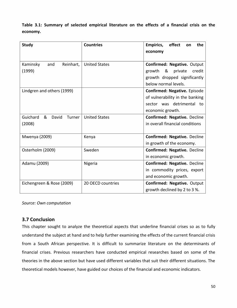
50
Table 3.1: Summary of selected empirical literature on the effects of a financial crisis on the
economy.
Study Countries Empirics, effect on the
economy
Kaminsky and Reinhart,
(1999)
United States Confirmed: Negative. Output
growth & private credit
growth dropped significantly
below normal levels.
Lindgren and others (1999) Confirmed: Negative. Episode
of vulnerability in the banking
sector was detrimental to
economic growth.
Guichard & David Turner
(2008)
United States Confirmed: Negative. Decline
in overall financial conditions
Mwenya (2009) Kenya Confirmed: Negative. Decline
in growth of the economy.
Osterholm (2009) Sweden Confirmed: Negative. Decline
in economic growth.
Adamu (2009) Nigeria Confirmed: Negative. Decline
in commodity prices, export
and economic growth.
Eichengreen & Rose (2009) 20 OECD countries Confirmed: Negative. Output
growth declined by 2 to 3 %.
Source: Own computation
3.7 Conclusion
This chapter sought to analyze the theoretical aspects that underline financial crises so as to fully
understand the subject at hand and to help further examining the effects of the current financial crisis
from a South African perspective. It is difficult to summarize literature on the determinants of
financial crises. Previous researchers have conducted empirical researches based on some of the
theories in the above section but have used different variables that suit their different situations. The
theoretical models however, have guided our choices of the financial and economic indicators.

51
Chapter Four
Research Methodology
4.1 Introduction
The previous chapter outlined the theoretical and empirical considerations of the effects of a financial
crisis on the economy and also provided a guideline of the variables to be used in the analysis. In this
chapter, we formulate an equilibrium model that explains the extent to which the chosen variables
representing an economy affected by a financial crisis will affect the real economy. The study uses a
model that has been reformulated to suit the financial conditions in South Africa to analyze the
impact of the financial crisis on the real economy of South Africa.
4.2 Model Specification
The approach taken in this study is to augment an index, similar to the one used by Guichard and
Turner, (2008) and Osterholm (2009), with a broader set of financial variables that will show the
financial conditions in the South African markets. To investigate how the financial crisis affected the
South African real economy, a partial equilibrium model will then be used. The model is constructed
based on the Keynesian theory of aggregate demand for an open economy discussed in the
theoretical literature review. Given that the ultimate effect is felt on growth, the study specifies the
economic growth function based on the presumption that exogenous shock would affect growth
through a change in demand variable such as investment and exports. However, the study will also
analyze in detail the effects of the crisis on exports and investment.
The following National Income Identity in an open economy forms the basis of our time series
analysis:
Y = C + I + G + (X – M)…………………………………………………………………………………………………….…….….. (4.1)
Where: Y is the Output, C is consumption, G is government expenditure, X are the exports and M are
the imports.
However, this model does not capture some economic variables which play significant roles in
determining output and therefore is remodeled to construct GDP function which incorporates unique
variables pertinent to South Africa. Gross domestic product can be expressed in terms of either

52
expenditure (demand) or production (supply). This study will define GDP in terms of expenditure
mainly due to the presumption that predominant constraints facing the economy and the external
shock effects are on the demand side. The model is based on the Keynesian model of aggregate
demand and is remodeled to capture the determinants of economic growth. Specifying the Gross
Domestic Product (GDP) as:
GDP= f (NX, CR, FCI, DA)……………………………………………………………………………………………………..………... (4.2)
In order to avoid any misrepresentation of empirical result, this section provides a description of all
variables appearing in the estimated equation and also explains the a priori expectations. All the
variables are converted to logarithms for the obvious reasons of obtaining elasticity coefficients on
these variables and minimizing the impact of outliers. The rate of the growth in GDP is thus expressed
in the form:
LGDP = α1 + α2 L DA + α3L NX + α4 L CR+ α5 FCI + εt …………………………………………………………………..….. (4.3)
Where:
LGDP is the logarithmic of gross domestic product. GDP is the total value of final goods and services
produced within a country over a period of time.
LDA is the logarithmic of domestic absorption and is directly related to GDP. This is calculated as the
summation of all income that is absorbed by the economy, that is,
DA=∑ (Consumption, Investment, Government Expenditure)
LNX are the net exports and are expected to have a positive relationship with GDP. This has been
empirically proven hence Ibrahim (2002) found that an increase in net exports will increase economic
growth.
LCR is the logarithmic of credit extension. This has a direct relationship with GDP and therefore α4 is
expected to be positive. An increase in credit extended to the private sector will lead to an increase in
investment and therefore a growth in output.

53
FCI is the financial conditions index. The construction of this index is outlined in the following section.
The impact of the existing financial conditions on economic growth is likely to be negative because of
the uncertain environment it creates. A higher index indicates worsening market conditions and this
would create uncertainties in the market therefore reducing investment demand and consequently
economic growth.
α1, α2, α3, α4, and α5 are the coefficients to be estimated.
εt = is an error term.
4.3 Data sources and characteristics of variables:
The data covers the start of the decade in which the financial crisis started and would therefore be
able to capture the various events that occurred in the decade that posed as important thresholds to
the lead-up of the crisis. The period gives a clear trend of what happened including policies
implemented in South Africa (e.g. National Credit Act) that could have a significant effect on the
findings of the study and also the beginning of the financial crisis. All raw data are of quarterly
frequency and are taken from the World Bank (World Economic Indicators), the Johannesburg Stock
exchange (JSE) and the South African Reserve Bank (SARB) electronic data delivery systems.
Real GDP was used as a proxy for economic growth. Domestic absorption was calculated as the sum
of consumption, investment and government expenditure. Credit extended to the private sector is
measured in millions of rand. FCI is a computed variable to show the market conditions in the
financial market. Yearly real Gross Domestic Product (GDP) of South Africa and United States of
America are used as a measure for their respective real incomes. The study uses real U.S.GDP as a
proxy for foreign income because it is South Africa’s major trading partner.
Trade data are available in value terms rather than volume for South Africa, although theory and
previous studies suggest that trade volume is a more appropriate measure than value. The trade
variables are also measured at current prices as this takes into account effects of price movements.
Because expected inflation cannot be precisely determined as it varies from individual to individual,
this study will use actual inflation of the preceding years as a proxy for expected inflation for the

54
period under study. All variables used in the empirical analysis are transformed variables by the use of
natural logarithms.
The Index
The purpose of a financial conditions index is typically either i) monitoring of financial markets, which
often can be done in real time since financial data typically are available on a very high frequency, or
ii) estimation of the impact of financial conditions on other parts of the economy. The primary
concern of this study is the effect of the financial crisis on the South African real economy. The choice
of variables included in the index is thus affected since a long enough series is needed to make
estimation both meaningful and reliable. According to Osterholm (2009), from an econometric point
of view, it should be beneficial to weight together the information from several financial variables into
one index. By using fewer variables in the model the relationship between financial markets and the
real economy can be modeled in a simpler and more robust way. This should generate better
estimates of the effect on the real economy as well as improved forecasts.
The study uses three variables to build the financial index: real short-term interest rate, changes in
real effective exchange rate and changes in the stock exchange index. The South African short real
interest is calculated by subtracting expected inflation in the past four quarters from the Treasury bill
rate Consumption and investment decisions of firms and households are both functions of the real
interest rate. Osterholm (2009) also argues that the currency of a country is usually affected by
interest rate movements since both financial and real sector activity are influenced by financing costs
and inflation expectations. However, there are times when real interest rates may change whilst
external factors are at the same time causing the currency to depreciate. Changes in the stock
exchange index benchmark the performance of the stocks. Developments in the stock market reflect
many factors. Falling stock prices during the crisis can be an indication of a reduced risk appetite as
investors dispose of stocks for safer assets. The macroeconomic consequence of falling asset prices is
that consumption will generally be lowered due to the lower wealth of households. It will also be
more expensive to raise capital for firms through new share issues (as the cost of equity capital rises
with falling share values), which puts downward pressure on investment.

55
The single index for the state of the South African financial markets is generated as follows:
1. Each of the raw time series (real short-term interest rate, changes in real effective exchange
rate and changes in the stock exchange index) data are standardized so that they have a mean
of zero and a standard deviation of one.
z= ∑(X-u)/δ………………………………………………………………………………………………………………………… (4.4)
2. They are then weighted together using weights of 1/3 for the three series. This is because they
are considered equally important for describing the financial conditions.
Specifying the financial conditions index:
rtreerWFCIn
t
()(1
γ)……………………………………………………………………………………………….……….. (4.5)
Where W= weight of financial variable, reer = changes in real effective exchange rate (standardized),
rt = short term interest rate (standardized) and γ = changes in stock exchange index (standardized).
These variables are perceived to be some of the most relevant when assessing the state of financial
markets and should also have predictive power for the real economy since they capture several
important aspects of how a financial crisis is transmitted to the real economy.
Once the model that links the economic growth to its potential determinants has been specified and
variables defined, the next step is to estimate the parameters of the specified model. There are
several methods of parameter estimation that involve several steps. This is the subject of the next
section.
4.4 An overview of estimation techniques for the study of effect of the Financial Crisis
on the Economy
Several techniques are available for parameter estimation, ranging from classical regression methods
to co integration based techniques. The classical regression methods are based on the assumption
that all the variables to be included in a regression are stationary but most economic series are not
56
stationary in their levels such that estimations based on this technique will be meaningless (spurious).
A preferred approach would be to difference the variables to mechanically turn them stationary but
this throws away useful long run information that may be in the data. This problem can be resolved
by the new generation of models based on co integration and error correction modeling. Unit root or
stationarity tests will be done on all the variables before proceeding with the tests for co integration
and estimation of parameters. In order to directly test for stationarity, the study will employ the
Augmented Dickey-Fuller test. There are also several co integration based methods and this study will
employ the Johansen technique as this technique has been proven to be the most powerful and
reliable.
Since the model used in this study is multivariate, there is likelihood of having more than one co
integrating vector. According Harris, (1995), the Johansen (1991, 1995) approach is preferred to other
techniques such as the Engle-Granger (1987) as it is able to take into account the underlying time
series properties of the data and is a systems equation test that provides estimates of all co
integrating relationships that may exist within a vector of non stationary variables or a mixture of
stationary and non stationary variables.
The Engle-Granger technique assumes that there is only one co integrating relationship. In this case,
the OLS estimation will be applicable only if there is only one co integrating vector. However since this
is unlikely to be the case, the Engle-Granger model will not be valid and will not be able to identify all
co integrating relationships.
In implementing the Johansen methodology, several steps have to be followed. The study follows the
“generic to specific” framework suggested by Hendrel et.al. (2000) as opposed to the traditional
“specific to general” framework. The first step in the estimation is unit root testing, to confirm
whether all the variables are suitable to be included for co integration. If a variable is not stationary, it
has to be differenced until it becomes stationary. The next step is performing co integration tests in
order to identify any long run relationships in the variables. A short run vector error correction model
is then estimated only if co integration is found. Lastly, residual diagnostic checks will be performed.

57
We review each of these steps in the following sections with the aim of considering alternative tests
that can be employed in each step and choosing those to be applied in this study.
4.4.1 Testing for stationarity/ Unit Root testing
A stationary series (weakly or covariance) stationary is that which has a constant mean and variance
for each given period of time and “the value of the covariance between the two time periods depends
only on the distance or lag between the two time periods, not on the time at which the covariance is
calculated” (Gujarati, 2003: 797). A series that is not stationary is referred to as non stationary. If a
series is non stationary, it must be differenced d times before it becomes stationary. It is then said to
be integrated of order d. This is denoted as I (d), where d is the order of integration. The order of
integration refers to the number of unit roots in the series, or the number of differencing operations
it takes to make a variable stationary. An I(0) series is a stationary one whilst an I(1) series contains
one unit root.
Classical regression models deal with the relationships between stationary variables, but most of the
economic indicators usually follow a non stationary path. The use of non stationary data will lead to
spurious results or the danger of running a nonsense regression. In such a case, the results will be
meaningless. The usual t-ratios will not follow a t-distribution and the F-statistic will not follow an F-
distribution. It is likely that significant t-ratios and a high R2 will be obtained even though the trending
variables are completely unrelated.
As a result, unit root or stationarity tests should be done on all the variables before testing for co
integration and estimating the parameters. There are several tests for stationarity including a visual
plot of the data, unit root test and those that directly test for stationarity, among others. This study
will make use of the augmented Dickey-Fuller which is discussed in the section below.
4.4.2 The Dickey Fuller (DF) and the Augmented Dickey Fuller test (ADF)
According to Gujarati (2003), the stationarity of a time series can be tested directly with a unit root
test. The Dickey-Fuller (DF) and the Augmented Dickey-Fuller (ADF) are the most frequently used unit

58
root tests. The objective of the DF test is to test the null hypothesis that in the following
equation:
y= β 2 t + ω yt-1 + vt……………………………………………………………………………………………………………………….. (4.6)
The hypotheses of for the above equation would be:
H0: Series contains a unit root (H0: ω =0)
H1: Series is stationary. (H1: ω <0)
In practice, models under the above hypotheses have three cases:
When there is a test for a random walk against a stationary autoregressive process of order
one (AR(1))
When there is a test for a random walk against a stationary (AR(1)) with a drift
When there is a test for a random walk against a stationary (AR (1)) with a drift and time
trend.
For ease of computation and interpretation, Dickey Fuller test employs the following equation:
Δy = β1 + β 2 t + ω yt-1 + vt ……………………………………………………………………..……………………………………. (4.7)
Where yt is the relevant time series, Δ is a first difference operator, t is a linear trend and vt is the
error term. The error term should satisfy the assumptions of normality, constant error variance and
independent (uncorrelated) error terms. According to Takaendesa (2006), the results based on the DF
test will be biased if the error terms are not independent in equation (4.7). A limitation of the DF test
is that it does not take account of possible autocorrelation in the error process or term (vt). To
accommodate for this weakness, the ADF can be used and this test ‘augments’ the test using m lags of
the dependent variable. By adding a lagged differenced term on the right-hand side in the DF
equation (4.7), this test corrects for high-order serial correlation. As a result, the ADF employs the
following equation:
Δy = β 1 + β 2 t + ω yt-1 +∑ ………………………………………………….……………………………….. (4.8)

59
Equations (4.7) and (4.8) can also be estimated without including a trend term (deleting the term β2 t
in the equation) and without a constant (leaving out β1 in the equation). The lags of Δyt now ‘soak up’
any dynamic structure present in the dependent variable, to ensure that vt is not auto correlated. In
both tests above, if the calculated statistic is less (in absolute terms) than the MacKinnon (1991, 1996)
values, which are used by the E-views software, the null hypothesis is not rejected and will therefore
mean that there is a unit root in the series. In other words, it means the time series is not stationary.
The opposite is true when the calculated statistic is greater than the MacKinnon critical value.
Like any other unit root tests, the Dickey-Fuller test has its own weaknesses. The test is weak in its
ability to detect a false null hypothesis. Gujarati (2003: 819) states that unit root tests have low power
if the process is stationary but with a root close to the non stationary boundary, that is, they tend to
accept the null of unit root more frequently than warranted. According to Thomas (1997: 410), this
lack of power means that the Dickey-Fuller test fails to detect stationarity when the series follows a
stationary process. This could occur either because the null hypothesis was correct or because there is
insufficient information in the sample to enable rejection.
4.4.3 Phillips Perron Tests (PP)
The Phillips Perron test (PP) is a generalization of the ADF test procedure that allows for fairly mild
assumptions concerning the distribution of the errors. The test regression is the AR(1) process:
Δyt-1 = α0 + γyt-1 + et
According to Brooks (2008),the PP test makes a correction to the t-statistic of the coefficient from the
AR(1) regression to account for the serial correlation in et whilst the ADF test corrects for higher order
serial correlation by adding lagged differenced terms on the right hand side.
4.4.4 Co integration and error correction modeling.
According to Gujarati (2003:830), the co integration of two or more series suggests that there is a long
run or equilibrium relationship between them. This means that even though the series themselves
may be non stationary, they will move closely together over time and their difference will be
stationary. Their long run relationship is the equilibrium to which the system converges over time and

60
the disturbance term can be interpreted as the disequilibrium error or the distance that the system is
away from equilibrium at time t.
A set of variables is defined as co integrated if a linear combination of the two is stationary. In order
to proceed to this stage, all the series of interest should be integrated of the same order, preferably
I(1). The reason for this is that if the series display level stationarity, or are I(0), standard regression
and statistical inference could be carried out, since there would be no problem of spurious
regressions. On the other hand, if they are integrated of different orders the norm used to be
difference all the variables to be included in regressions. Harris (1995: 80), however, shows that it is
not necessary for all the variables in the model to have the same order of integration, especially if
theory a priori suggests that such variables should be included. Thus, a combination of I(0), I(1) and
I(2) can be tested for co integration.
According to Brooks (2002:387), in most cases, if two variables that are I(1) are linearly combined,
their combination would also be I(1). More generally, if variables with differing orders of integration
are combined, the combination would have an order of integration equal to the largest. The exception
to this rule is when the series are co integrated.
There are two broad categories of co integration: those that are residual based, such as the Engle-
Granger approach and those that are based on maximum likelihood estimation on a VAR system, such
as the Johansen method.
Engle and Granger (1987) came up with a four step procedure to determine if two I(1) variables are co
integrated of the order(1,1). The test is applied on the residuals and the initial step includes pre-
testing the variables for their order of integration. Co integration of the variables necessitates that the
two variables be integrated of the same order. The second step involves estimating the long run
equilibrium relationship.
According to Choga (2008:81), the null hypothesis states that there is unit root in the potentially co
integration regression and the alternative hypothesis states that the residuals are stationary. If the

61
null is rejected, the conclusion drawn is that a stationary linear combination of the non-stationary
variables has been found. The variables would therefore be classified as co integrated. If, however,
the null is not ejected, it means that there is no co integration.
The third step involves estimating the error correction model. If the variables are co integrated, the
residuals from the equilibrium regression can be used to estimate the error-correction model. Finally,
the model is assessed for adequacy.
The Engle-Granger approach suffers from numerous problems when applied to multivariate models.
According to Harris, (1995: 76), such problems include the usual finite sample problem of a lack of
power in unit root and co integration tests and the inability to detect more than one co integrating
relationships that may exist in a model. Since our model is multivariate, there is a likelihood of having
more than one co integrating vector. The Engle-Granger approach would therefore produce
inconsistent estimates. Thus, in light of these problems, we prefer the Johansen methodology.
4.4.5 Johansen technique based on VARS
According Harris, (1995), the Johansen technique has several advantages over other co integration
techniques. The main objective of these co integration tests is to determine whether the variables in
our economic growth model are co integrated or not. The presence of a co integration relation(s)
forms the basis of the vector error correction model (VECM) specification. Identifying the number of
co integration vectors within the VAR model is the basis for this procedure. To identify the number of
co integration vectors a likelihood ratio test of hypotheses procedure is used. The Johansen
procedure consists of four steps:
1. Set the appropriate lag length of the model
The lag length test is used to find the number of lag values that should be included in the model. The
Johansen test can be affected by the lag length employed in the VECM. It is therefore crucial to
attempt to select the lag length optimally. The lag length that is chosen should produce the number
and form of co integration relations that conform to all the a priori knowledge associated with
economic theory. According to Brookes (2002:334), multivariate versions of the information criteria,

62
which includes the sequential modified likelihood ratio (LR), Akaike information criterion (AIC), Final
prediction error (FPE) Schwarz information criterion (SIC) and the Hannan-Quinn information criterion
(HQ) can be used to determine the appropriate lag length.
2. Choose the right model regarding the deterministic components in the multivariate system
The choice of deterministic components requires that all variables be pre-tested to assess the order of
integration. It is easier to detect the possible trends when a series is plotted. The order of integration
is important, because variables with different orders of integration pose problems in setting the co
integration relationship. Order of integration is detected by the unit root test discussed earlier. the
graphical analysis of the raw data and unit root tests, together with a priori knowledge from economic
theory, should assist in selecting the deterministic trend assumption to be used in the Johansen test
for co integration (rank of Π ).
3. determination of the rank of Π
This step involves determining the number of co integrating vectors. The model considered for co
integration can be estimated in several forms based on the specification of the constant and the time
trend. If the model has a constant without a time trend, then it can be estimated in two forms: either
the constant is inside the co integrating vector, or it is outside the co integrating vector. If the model
has a time trend, then it is considered either inside or outside the co integrating vector.
It is important to evaluate whether the results of the analysis have a sound economic base. Apply
causality tests on the error correction model to identify a structural model and determine whether
the estimated model is reasonable.
Assuming a set, n, of variables [LGDP, LDA, LCR, DLNCA, and FCI] that are integrated of order one, I
(1), are thought to be cointegrated. A VAR with k lags could be set up:
………………………………………………………………………………………….(4.9)

63
The Y’s are n x 1 vectors of deterministic variables, and the coefficient estimates are contained in n x n
matrices. To use the Johansen test, the VAR now needs to be turned into a vector error correction
model (VECM) Yt of the form:
( ) ………………………………………………………(4.10)
On the LHS, the above VAR contains n variables in first difference form, a lag in the dependant
variable and k-1 lagged differences of the dependant variables on the RHS. Because the Johansen test
is sensitive to the lag length employed, the optimal lag length should be determined as described
earlier.
The Π matrix can be interpreted as the long-run coefficient matrix; in the long-run equilibrium all the
RHS lagged terms in Yt should be zero and, setting ut = 0, ΠYt-k must equal zero so that Yt has settled at
its equilibrium level. It is thus the Π matrix that is of concern in testing for co integration.
The test for co integration between the Ys is calculated by looking at the rank of the Π matrix via its
eigenvalues. The rank of a matrix is equal to the number of its characteristic roots (eigenvalues) that
are different from zero or the maximum number of linearly independent rows or columns contained
in the matrix; a full rank matrix is one where its rank is equal to its dimensions, and reflects no linear
dependence at all in the rows or columns. Intuitively, the lower the rank of the matrix the greater will
be the number of linearly dependent rows and/or columns in the matrix.
The characteristic equation of the matrix Π is given by:
| |…………………………………………………………………………………………………………………………………….. (4.11)
Where In is an identity matrix and the ’s are the characteristic roots (obtained by factorization). The
characteristic roots are also known as the eigenvalues, and the sum of the eigenvalues is the trace of
the matrix.
Two test statistics for co integration are employed under the Johansen technique and are formulated
as:

64
• trace (r ) = -T ∑ ( ) This is a joint test where the null is that the number of co
integrating vectors is equal to or less than r, with the alternate being a general test that this
number is greater than r.
• max (r+1)= - T ( ) This is a separate test on each eigenvalues, where the null is that the
number of co integrating vectors is equal to r against the alternative of r + 1.
r is the number of co integrating vectors under the null hypothesis and T is the sample size. Testing is
conducted sequentially, starting with r = 0 and increasing r by one at a time. In each of the above
cases, the null is rejected if the test statistic is greater than the critical value and the test is repeated
at the next level of r. If the null cannot be rejected at any time then the testing process would be
complete. The Johansen technique allows for hypothesis testing regarding the equilibrium
relationships, and these are conducted by imposing restrictions on the matrix.
5. Estimating the VECM
The last and final step involves estimating the VECM if co integration is found. This is done by
specifying the number of co integrating vectors, trend assumption used in the previous step and
normalizing the model on the true co integrating relation(s). Thus, a VECM is merely a restricted VAR
designed for use with non stationary series that have been found to be co integrated. The specified co
integrating relation in the VECM restricts the long run behavior of the endogenous variables to
converge to their co integrating relationships, while allowing for short run adjustment dynamics. Once
estimation is complete, the residuals from the VECM must be checked for normality, heteroskedacity
and autocorrelation.
4.4.6 Error correction model (ECM)
The error-correction mechanism corrects for disequilibrium in the short-run. The Granger
Representation Theorem states that, if two variables X and Y are co integrated, then the relationship
between the two can be expressed as an ECM. According to Enders (2004:329), in an error-correction
model, the short-run dynamics of the variables in the system are influenced by the deviation from
equilibrium:

65
( ) …………………………………………………………………………………….. (4.12)
Where: this is the characteristic “error correction” specification, where the change
in one variable is related to the change in another variable, as well as the gap between the variables
in the previous period. The term gives the error correction term. According to Brooks
(2002:389), a necessary condition is that Yt and Xt are co integrated with the co integrating coefficient
γ then will be I(0) even though the constituents are I(1). It will then be possible to use
the OLS and standard procedures for statistical inference on the equation above. It is also possible to
add an intercept in either the co integrating term or in the model for ΔYt.
ECMs can be interpreted as follows: Y is supposed to change between-1 and as t as a result of changes
in the values of the explanatory variables, the Xs between t-1 and t and also in part to correct for any
disequilibrium that existed during the previous period. The error correction term has to appear with a
lag for it would not be reasonable for it to appear without one. This would imply that Y changes
between t-1 and t in response to a disequilibrium at time t. The long-run relationship between x and y
is defined by γ whilst β1 describes the speed of adjustment back to the equilibrium. Its strict definition
is that it measures the proportion of last period’s equilibrium error that is corrected for. The ECM can
therefore be measured for more than two variables.
4.4.7 Advantages of ECM
ECM is a convenient model measuring the correction from disequilibrium of the previous period and
this has a very good economic implication. The model is also formulated in terms of first differences
which typically eliminates trends from the variables involved and solves the problem of spurious
regressions. ECMs also easily fit into the general to specific approach to econometric modeling, which
is in fact a search for the most parsimonious error correction mechanism that best fits the given data
sets. The error correction model is also particularly powerful since it allows an analyst to estimate
both short term and long run effects of explanatory time series.

66
4.5 Diagnostic Checks
The following section is a very crucial stage in the analysis of the effects of a financial crisis on the
economy as it confirms parameter estimation outcomes achieved by the estimated model. Diagnostic
checks test the stochastic properties of the model, such as residual autocorrelation,
heteroscedasticity and normality, among others.
4.5.1 Autocorrelation test: Lagrange Multiplier (LM)
The term autocorrelation may be defined as “correlation between members of series of observations
ordered in time. Lagrange Multiplier (LM) test which is a multivariate test statistic for residual serial
correlation up to the specified lag order. The LM test is formulated as below:
TR2 ≈ χ2 (m)
Where: m is the number of regressors in the auxiliary and T is the number of observations. The test
centers on the values of the R2 for the auxiliary regression and the test statistic for the chosen lag
order (m) is computed by running an auxiliary regression of the residuals (μt) on the original right-
hand explanatory variables and the lagged residuals (μt−m) and multiplying it by the number of
observation, T. If at least one of the coefficients in an equation is statistically significant, the value of
the R2 will be relatively significant. According to Harris (1995: 82), the lag order for this test should be
the same as that of the corresponding VAR. The LM statistic tests the null hypothesis of no serial
correlation against an alternative of auto-correlated residuals.
4.5.2 White Heteroscedasticity Test
White’s (1980) general test of heteroscedasticity tests the null hypothesis that the errors are both
homoskedasticity (no heteroscedasticity problem) and independent of the regressors and that there
is no problem of misspecification. The test regression is run by regressing each cross product of the
residuals on the cross products of the regressors and testing the joint significance of the regression.
The null hypothesis for the White test is no heteroscedasticity and misspecification. If we fail to reject
this null, we have homoskedasticity. The failure of any one or more of the conditions just mentioned
above could lead to a significant test statistic.

67
4.5.3 Residual Normality Test
The normality test is used to find out whether the random variable is normally distributed or not. This
test is applied to residuals from a linear regression model. If they are not normally distributed, the
residuals should not be used in Z tests or any other tests derived from the normal distribution such as
F-tests and the chi-square test. The residual normality test used in this study is the multivariate
extension of the Jarque-Bera normality test, which compares the third and fourth moments of the
residuals to those from the normal distribution. The preferred residual factorization method for the
test is by Urzua (1997), which makes a small sample correction to the transformed residuals before
computing the Jarque-Bera statistic. The joint test is based on the null hypothesis that residuals are
normally distributed. A significant Jarque-Bera statistic, therefore, points to non-normality in the
residuals. However, the absence of normality in the residuals may not render co integration tests
invalid.
4.6 Conclusion
This chapter specified the variables that would potentially transmit the effects of the financial crisis
onto the economy and explained the approach to be used in obtaining the regression results for the
study. The technique for parameter estimation that is going to be used in this study was also
discussed and this is the Johansen technique. To validate the parameter estimation outcomes
achieved by the model, diagnostic checks will also have to be carried out. These checks test for the
stochastic properties of the model, such as heteroscedasticity, autocorrelation and residual normality
and include the White test, Durbin Watson test and the Jarque-Bera normality test respectively.

68
Chapter Five
Presentation and Analysis of Results
5.1 Introduction
This chapter applies the techniques discussed previously to South African data in order achieve the
objectives set out in chapter 1. This chapter augments the analysis by applying that framework and
the analytical techniques proposed on quarterly South African data covering the period 2000 to 2009.
The results presented include those of unit root tests, co integration test and finally the regression.
Stationarity co integration and tests will be done in order to establish the long run relationship.
Thereafter, the error correction model will be estimated. The econometric package used in this study
is E-views version 6. The following section will present the empirical findings.
5.2. Empirical Findings
The following section is divided into four sub-sections. The first presents the results of
stationarity/unit root tests, the second presents and discusses the co integration test results; the third
discusses the long run relationship and presents the results from the analysis. Diagnostic checks
results are provided in the fourth sub-section.
5.2.1 Stationarity results
Determining the order of integration of the series is the first step of the Johansen methodology and in
this study, three tests for stationarity are employed including an informal one which is the graphical
analysis of the series. A visual plot of the series is important and is usually the first step in the analysis
of any time series before pursuing any formal tests. This allows the detection of any data capturing
errors, and structural breaks or drifts that may bias the unit root tests and gives an idea of the trends
and stationarity of the data set. The other two tests are used simultaneously as one test may not be
fully reliable. If they give different results, the stronger one of the two is considered. The Phillip-
Perron tests have been found to be more powerful than the augmented Dickey-Fuller test in finite
samples. The figure below shows plots of all variables used in the model.

69
Figure 5.1 Stationarity graphs
The visual plot above shows that apart from the financial conditions indexFCI, all the other variables
have unit root present at level. The net exports variable seems to be slightly stationary. Although the
amplitude is wide, the variable oscillates around the mean of zero.
-8
-4
0
4
8
12
00 01 02 03 04 05 06 07 08 09
FCI
5.7
5.8
5.9
6.0
6.1
6.2
6.3
6.4
00 01 02 03 04 05 06 07 08 09
LCR
5.2
5.3
5.4
5.5
5.6
5.7
5.8
00 01 02 03 04 05 06 07 08 09
LDA
5.9
6.0
6.1
6.2
6.3
6.4
00 01 02 03 04 05 06 07 08 09
LGDP
-30,000
-20,000
-10,000
0
10,000
20,000
00 01 02 03 04 05 06 07 08 09
NX

70
Stationarity graphs after 1st differencing
To solve the unit root problem, the variables were differenced and after differencing once, all
variables become stationary. This means that they are integrated of order one, that is, they are I(1).
The formal tests employed, as mentioned above, are the Augmented Dickey Fuller test (ADF) and the
Phillips Peron. These are used to identify the order of integration i.e. the number of times a variable
needs to be differenced to make it stationary. Below is table 5.1 that presents stationarity results for
South Africa. These were arrived at after a number of preliminary trials.
-12
-8
-4
0
4
8
12
00 01 02 03 04 05 06 07 08 09
DFCI
-.01
.00
.01
.02
.03
.04
.05
00 01 02 03 04 05 06 07 08 09
DLCR
-.02
-.01
.00
.01
.02
.03
.04
00 01 02 03 04 05 06 07 08 09
DLDA
.000
.005
.010
.015
.020
.025
.030
00 01 02 03 04 05 06 07 08 09
DLGDP
-15,000
-10,000
-5,000
0
5,000
10,000
15,000
00 01 02 03 04 05 06 07 08 09
DNX

71
Table 5.1: Stationarity test results
** represents a stationary variable at 1% significance level
* represents a stationary variable at 5% significance level
The table and graphical analysis above present the stationarity tests for the South African variables
used for the regression analysis. Some of the variables were first entered in their log values and the
ADF and Phillips Peron results were obtained. The above results show that only FCI is not stationary
at level with no constant and trend, with a constant only but is stationary with both a constant and a
trend at 1% significant level in both tests. LDA is stationary at level with a constant and trend at 5%
significant level in the ADF test and NX is stationary at level with a constant and trend at 1%
Augmented Dickey Fuller test Phillips Peron I
Variable None Intercept Trend &
Intercept
None Intercept Trend &
Intercept
FCI -1.184 -2.256 -5.177** -1.184 -2.240 -5.163** I(1)
LCR 8.052 -0.002 -1.516 6.587 -0.077 -1.725 I(1)
LDA 6.467 -0.453 -3.455* 13.906 -0.522 -3.512 I(1)
LGDP 12.548 -1.035 -1.827 11.539 -0.986 -2.120 I(1)
NX -1.803 -1.840 -3.139 -1.803 -1.840 -2.984** I(1)
DFCI -10.327** -10.210** -10.076** -20.427** -20.653** -17.118** I(0)
DLCR -2.309* -4.322** -4.212** -2.026* -4.327** -4.216* I(0)
DLDA -4.031** -7.859** -7.746** -3.985 -12.545** -12.005** I(0)
DLGDP -1.863 -4.910** -4.910** -1.579 -4.807** -4.806** I(0)
DNX -9.685** -9.578** -9.499** -9.776** -9.673** -9.589** I(0)
Critical
value
5%
-1.952 -2.956 -3.557 -1.950 -2.941 -3.533
Critical
value
1%
-2.637 -3.650 -4.271
-2.627 -3.616 -4.219

72
significant level in the Phillips Peron test. The rest of the variables LGDP, LCR and NX are not
stationary at level in all forms.
All variables however become stationary in their 1st differences in both the ADF test and the Phillips
Peron test. All variables are stationary where there is only a constant. DFCI, DLDA and DNX are
stationary in all forms at 1% significant level after being differenced only once. According to the ADF
test, both DLCR and DLGDP are stationary at 1% significant levels with a constant only and where
there is a constant and a trend. However, only DLCR is stationary at 5% significance level where there
is neither a constant nor a trend and DLGDP is not. The Phillips Peron test shows that after
differencing; only DLDA and DLGDP remain non stationary where there is no constant. The rest of the
variables are stationary at 1% significance levels in all forms except DLCR which is stationary at 5%
significance level where there is a constant and trend.
The ADF results are in line with the graphical analysis. We therefore conclude that all of the series are
of the I(1) order of integration therefore the investigation of the co integration properties is the next
step. We then move on to do the co integration tests in the following section.
Co integration
Co integration analysis is conducted using the Johansen procedure to determine whether there is a
long run equilibrium relationship between the gross domestic product and its theoretical
determinants thus enabling the formulation of an error correction model. The advantage of this
approach is that it allows one to integrate the long-run and the short-run relationship between
variables within a unified framework. There are two conditions that have to be met for two or more
variables to be co integrated. The first one is that they have to be of the same order of integration.
Secondly, linear combinations of the variables from the regression of the non stationary variables (in
level) must be stationary. According to Brooks (2008), co integrated variables ensure that we
eliminate spurious relations and as such share common stochastic trends. Now that we have
established that our variables are integrated of the same order, table 5.2 that follows shows the co
integration test results for the variables we used.

73
Lag Length selection
The choice for the lag order for the VAR was made using the information criteria approach such as the
Schwarz and Akaike information criteria as well as the Likelihood Ratio (LR) test amongst others,
augmented by theoretical priors. Johansen’s co integration approach has been criticized for being
sensitive to the lag length chosen therefore important that a consistent procedure is used to choose
the lag length for both the co integration analysis and the error correction model. When the lag
lengths chosen by all information criteria are the same, this lag length will be used for both the co
integration analysis and error correction model. Below is a table that shows the results of the lag
length selection criteria.
Table 5.2 VAR Lag Order Selection Criteria
VAR Lag Order Selection Criteria
Endogenous variables: LGDP Exogenous variables: C FCI LCR LDA NX
Date: 07/23/10 Time: 15:25
Sample: 2000Q1 2009Q4
Included observations: 35 Lag LogL LR FPE AIC SC HQ 0 123.365 NA 6.78e-05 -6.764 -6.542 -6.687
1 136.144 21.177* 3.46e-05* -7.437* -7.170* -7.345*
2 136.959 1.303 3.51e-05 -7.426 -7.115 -7.319
3 137.333 0.577 3.64e-05 -7.390 -7.035 -7.268
4 138.110 1.155 3.70e-05 -7.378 -6.978 -7.240 * indicates lag order selected by the criterion
LR: sequential modified LR test statistic (each test at 5% level)
FPE: Final prediction error AIC: Akaike information criterion
SC: Schwarz information criterion
HQ: Hannan-Quinn information criterion
The lag that produces the best-behaved model in terms of diagnostic test will be chosen for the error
correction model. Based on the results presented in table 5.2 above, a lag length of 1 was chosen.
The trace and maximum eigenvalues tests are undertaken to investigate the number of co integrating
vectors in the model. Table 5.3 below presents the Johansen co integration test based on the trace
test and on the maximum eigenvalue test.

74
Table 5.3: Co integration test results
Trace Statistic Trace Statistic Maximum Eigen Value
Statistic
HO:
Rank = ρ
λ -Tlog(1- λ) λTrace95% -Tlog(1- λ) λmax95%
ρ=0 0.694 88.604** 69.819 41.468** 33.877
ρ<1 0.533 47.136 47.856 26.650 27.584
ρ<2 0.279 20.487 29.797 11.433 21.132
ρ<3 0.194 9.054 15.495 7.565 14.265
ρ<4 0.042 1.489 3.841 1.489 3.841
Values marked with * represent a stationary variable at 5% significant level and ** represent a
stationary variable at 1% significance level.
The results of the trace test rejects the null hypothesis of no co integrating vectors, since the test
statistic of about 88.6 is greater than the 1 per cent critical value of approximately 69.8. The trace
test, therefore, concludes that there is a co integrating relationship (vectors) at the 5 per cent level of
significance. The maximum eigenvalue test gives similar results and rejects the null hypothesis of no
co integrating vectors, since the test statistic of about 41.5 is greater than the 1 per cent critical value
of approximately 33.9. The maximum eigenvalue test also gives the same results for the economic
growth model. The co integrating relationship can be shown graphically as below.
Co integration graph
The results presented above can be confirmed by plotting graphs of co integration vectors as shown
in the figure below. The vector in the co integrating equation appears to be relatively stationary.

75
Co integration graph
Having established the existence of a long run relationship between gross domestic product, credit
extended, domestic absorption and net exports, the short run and long run dynamics of the model
can now be established with an error correction model.
5.3 The Error Correction Model (ECM)
The ECM technique allows the long run and short run dynamics to be estimated in a single step. The
single error correction framework has a constant which is a combination of the long run and the short
run constant thus isolating the speed of adjustment parameter which indicates how quickly the
system returns to equilibrium after a random shock. The general-to-specific strategy was used and
insignificant variables were sequentially eliminated, leading to a parsimonious specification.
-.3
-.2
-.1
.0
.1
.2
2001 2002 2003 2004 2005 2006 2007 2008 2009
Cointegrating relation 1

76
Table 5.4 Regression results on SA GDP growth rate
INDEPENDENT VARIABLES COEFFICIENT T-VALUE
CONSTANT -0.476 -2.59***
DLCR 1.555** 1.380*
DLDA 2.665** 1.866**
DFCIt-1 -0.863 -3.825***
DNXt-1 0.063 1.930**
ECTt-1 -0.129 -3.462***
Number of observations: 35
Adjusted R2 0.890
Note: Values marked with * represent a stationary variable at 10% significant level and **
represent a stationary variable at 5% significance level and *** represent a stationary variable
at 1% significance level.
Firstly, we look at effect of the financial market conditions on growth. This is the variable of interest in
this study. The country’s financial conditions, as represented by the index FCI have a negative effect
on the country’s economic growth. The variable carries an expected negative sign. The coefficient
suggests that a 1% deterioration of the conditions in the financial market will result in a decrease in
economic growth by about 0.863. The impact of financial crisis is highly significant indicated by the
high coefficient and significant level of 1%. Theory does postulate a negative relationship between the
financial conditions of a country and its economic growth and thus the variable bears the expected
sign. Guichard and Turner (2008) found results almost similar to this; they found that economic
growth slowed down due to worsening of the financial markets conditions.
According to an FNB economist, Nxedlana (2009), the impact of the credit and confidence crisis
intensified during the financial crisis. The negative consequences on real economic activity in the
industrialized were felt greatly in other countries. Some of the world’s largest economies were driven
into simultaneous recession. The variable CR represents the credit extended to the private sector.
Increasing the credit extended to the private sector will push investment upwards as more loans
become available. This will consequently lead to an increase in output. For that reason, supply of

77
credit to private sector has a direct relationship with GDP and is therefore expected to have a positive
sign. This variable is correctly signed and suggests that in the long run, a 1% increase in credit
extension will result in approximately 1.555% increase in economic growth. Significance of the
variable was at 10% suggesting that credit extension did not play a major role on the reduction of
economic growth in South Africa.
DA is a measure of domestic absorption and comprises investment, consumption and government
expenditure. As expected, this has a correct positive coefficient of 2.665 which suggests that an
increase in domestic absorption by 1% will lead to an increase in output by approximately 2.66%. This
variable is significant at 1% indicating that it has significant impact on economic growth and this
conforms to economic theory.
According to Dornbusch (1991), trade facilitates access to new goods, adoption of new methods of
production, and the new organization of industries. Theory therefore postulates a positive
relationship between net exports and economic growth. The variable net export (NX) in this study
carries a correct sign. A priori, this variable is expected to be directly varying with economic growth.
The results suggest that a 1 unit increase in net exports will result in economic growth increasing by
approximately 0.063. The t-value and p-value both show a significant level of 5%.
The error correction term for this model shows that only 13% of the equilibrium error is corrected in
one quarter. This means that it will take almost a 2years for full equilibrium to be reached. The speed
of adjustment is relatively slow. This is mainly because the shock to the system was an exogenous one
and therefore beyond the control of the South African government. Full recovery will also depend on
the recovery of the global economy. The sign is negative therefore conforms to economic theory and
it is significant at 1%. The South African Reserve Bank government is still trying to correct the negative
effects the financial crisis had on the growth of the economy.
The results of the economic growth model that was estimated and tabulated in table 5.4 above were
obtained using quarterly data on five variables. As shown by the high adjusted R2 of 0.890428, data is
robust. The adjusted R2 measures the closeness of fit of the regression model and reveals that the

78
statistical fit of the model is satisfactory. The model was also subjected to a number of diagnostic
tests. These checks are crucial in this analysis, because if there is a problem in the residuals from the
estimation of a model, it is an indication that the model is not efficient, such that parameter
estimates from such a model may be biased. Of importance in this analysis are the residual diagnostic
checks for serial correlation, normality and heteroscedasticity. Results from the diagnostic tests
performed in this study are presented in Table 5.5 below.
Diagnostic checks: Table 5.5
Test Test statistic P-value
Autocorrelation (LM) 24.01 0.51
White Heteroscedasticity Test 245.76 0.24
Normality (Jarque-Bera) Chi2(2) = 1.352 0.508
As mentioned in Chapter 4, the three tests are based on the null hypothesis that there is no serial
correlation, there is normality (keeping in mind the CLRM assumption that the residuals are normally
distributed with a mean of zero and a constant variance and that a violation of this assumption leads
to inferential statistics of a regression model) and there is no heteroscedasticity problem for the LM,
Jarque-Bera and White heteroscedasticity tests, respectively. The results of the test reveal that the
model is relatively well specified.
5.4 Conclusion
This chapter analyzed the impact of the financial crisis on the economy. Based on theory, a
background on the financial crisis and South African economy and data availability, an economic
growth model was specified. The potential explanatory variables included in this model include the
financial conditions index, domestic absorption, credit extension and net exports. The chapter started
by analyzing the time series properties of the data employing both informal and formal tests for
stationarity. The Johansen (1991, 1995) co integration technique was chosen as the preferred
parameter estimation technique for the economic growth model because of its several advantages
over alternative techniques. The variables were found to be integrated of the same order and the test
provided evidence of one co integrating relationship. Finally, the economic growth model was

79
estimated and the regression results were produced. The regression results from the model support
the notion that a financial crisis has a negative impact on the growth of the economy. These results
were supported by economic theory and empirics. The model was also subjected to diagnostic checks
and results indicated that the model was robust.

80
Chapter Six
Conclusions, Policy Implications and Recommendations
6.1 Summary and conclusions
This chapter attempts to draw conclusions and give policy implications and recommendations based
on the results obtained in the previous chapter. The study investigated the impact of the financial
crisis on the South African economy in the period 2000Q1-2009Q3. The macroeconomic background
for the country was presented and literature surrounding impact of financial crises and empirics of
past crises were also explained in the study.
Based on an extensive review of literature on the effects of financial crisis on the economy and on
data availability, an empirical model that links economic growth and its potential determinants was
specified. The variables used included domestic absorption, net exports, credit extension and financial
conditions in the market. The Johansen co integration and error correction methodology was used
because of its advantages over other techniques. The first step employed was the analysis of the time
series properties of the data by employing both formal and informal tests for stationarity. The
variables were found to be integrated of the same order and all of them were stationary after being
differenced once. Evidence of one co integrating relationship was established by the Johansen co
integration test and this allowed for the estimation of VECMs which provided parameter estimates for
the long run relationships.
The study revealed that the financial conditions in the market are negatively related to economic
growth. This means that if conditions in the financial markets worsen, growth of the economy
deteriorates. The financial condition index coefficient was highly significant at 1% significant level
revealing that the financial crisis had a significant effect on the South African economy. All the other
variables which include domestic absorption, net exports, credit extension were positively related to
the growth of the economy.
An interesting parameter in the VECM is the speed of adjustment coefficient. This measures the
speed of adjustment in the economy following a shock in the system. The study revealed that about

81
13% of the variation in output from its equilibrium is corrected within a quarter, meaning it takes
about two years for full equilibrium to be reached after the shock in the system has occurred.
Although the financial crisis did affect the South African economy, the impact was by far less than the
impact on other economies whose markets were not fully protected and regulated. This however
does not necessarily imply an easy task for the South African authorities as a lot still needs to be done
to restore the country’s equilibrium.
6.2 Recommendations and Policy Implications
This research makes a contribution to the policy debate by examining whether or not the financial
crisis was responsible for the decline in the growth of the economy and also whether the effect was
significant or not. The South African economy experienced sluggish economic growth during the
period of the crisis although it was not significantly affected by it. When the crisis occurred, South
African financial markets were relatively healthy and well insulated by regulation laws and supervision
such as (Credit Act and Basel II implementation) and therefore have not been as severely exposed to
toxic loans as its international counterparts. This is why the impact of the crisis was miniature.
However, since the crisis, the SA financial, foreign exchange markets including markets for commodity
exports declined. In addition, risk premium increased and the stock market’s overall index also fell,
but the fall was lower than the decrease in emerging markets index. The rand came under pressure in
line with experiences in other resource-dependent emerging markets running current account
deficits.
The performance of the country’s gross domestic product growth up to the second quarter of 2008
was mainly influenced by domestic developments such as interest rates hikes and power shortages, as
well as vigorous growth in commodity prices. With the commodity price implosion and escalating risk
aversion, South Africa only started to feel the impact during the third quarter of 2008. Consequently,
the economy weakened due to a significant decline in manufacturing sector and recorded the lowest
growth rate in ten years.

82
The policy stance adopted by any government may differ from country to country because of the
different financial, political or economic situations that may exist in a particular country. The South
African Reserve bank has to take into the consideration these characteristics before making a move.
The government has various options in dealing with the effects of the crisis. Considering the
importance of financial assets in the financial economy, the South African Reserve Bank can also
intervene in the money market by accommodating the increased borrowing pressure and thus
avoiding or reducing the pressure on interest rates; this will shift the burden of adjustment onto the
exchange rate. SARB can intervene in the spot and/or forward exchange markets to reduce pressure
on the exchange rate and shift the burden of adjustment onto interest rates. Keeping in line with
international policy guidelines, the financial stability of the Bank can identify and monitor excessive
domestic credit extension that could result in self-feeding asset-price bubbles.
In an effort to cushion the economy from the impact of the recent and future financial crises, the
SARB should intensify its pursuit of a conscious macro-prudential framework. This would limit
financial system-wide distress that will result in significant losses in terms of real output. The
authorities should adopt countercyclical policies that will foster discipline during upward and
downward phases of the business cycles. These policies should help to smooth the effects of
economic cycles, lessen unintended consequences and direct the reaction of commercial banks and
those of other financial institutions towards rational decision-making, rather than fuelling and
reinforcing a particular cyclical phase.
In my opinion, the results obtained in the study have two policy implications: Firstly, the presence of
the long run co-movements between the economy and its determinants found in the study implies
the effectiveness of targeting one of the variables in influencing the behavior of the other variables.
Supposing that this interpretation holds, this then justifies the stance taken by SARB in manipulating
interest rates (and consequently the FCI and the credit extended to the private sector) in order to
influence the long run behavior of the other variables that also affect the economy.
83
Secondly, the South African economy may be affected by external shocks that are outside the control
of the authorities. The policy implication is that the authorities will have limited influence on the
extent to which the financial crisis impacts on the economy.
It is difficult to fully escape the impact of financial crises of this nature because of the international
relationship that exists between countries and the global environment in which they operate.
Financial crises of this nature therefore should always be a cause of concern especially for relatively
small economies like South Africa and thus stringent regulatory measures should always be in place to
avoid severe effects when these crises do occur.
6.3 Limitations of the study and areas for further research
The study focused on selected macroeconomic variables determining economic growth. This may
have left other important variables, such as power shortages, that may affect the growth of the
economy. This work only considered the period from the start of the decade in which the global
financial crisis began up to the current period. The study will be limited to the South African economy
only and the consequence is that the results obtained may not be applicable to other economies.
However the study remains significant as the conclusions drawn from it may prove to be useful in the
South African context.
The study mainly focused on the effect of financial crisis on growth of the economy as a whole.
Certain sectors of the economy may have been adversely affected which may not have been reflected
by the growth rate of the economy. Therefore, from this aspect a useful extension of this study can
be made.

84
7.0 References for dissertation
Akkas, A. 2009, Review of Global Financial Crisis 2008: Issues, Analytical Approaches and
Interventions. Bangladesh: Bangladesh Open University
Allen, F., & Gale, D. 2007. The Anatomy of Financial Crises: Understanding Their Causes and
Consequences. Knowledge @Wharton: Wharton School of the University of Pennsylvania.
Binaku, I & Holstrom, N. 2009. The anatomy of financial crises and the current one’s effects on the
Swedish Economy. Sweden: Umea School of Business. Bachelor thesis.
Bordo, M.D 2009. The Great Contraction and the Current Crisis: Historical Parallels and Policy
Lessons. Shadow Open Market Committee Symposium: April 24, 2009, 2-7.
Bordo, M.D., Meissner, C.M & Stuckler, D. 2009, Foreign Currency Debt, Financial Crises and
Economic Growth: A Long Run View. NBER Working Paper 13577. November
Branson, W.H. 1989. Financial Market Integration and Monetary Policy in 1992.Working paper,
Marstrand, September.
Braun, M & Larrain, B. 2005. "Supply matters for asset prices: evidence from IPOs in emerging
markets," Working Papers 06-4, Federal Reserve Bank of Boston.
Brooks, C., 2002. Introductory econometrics for finance. Cambridge: Cambridge University Press.
Burda, M. & Wyplosz, C. 2005. Macroeconomics (2e). New York: Oxford University Press.
Choga, I., 2008. An Empirical Analysis of the Determinants and Growth of South African Exports.
East London: University of Fort Hare (M.Com-thesis).
Claessens, S & Thomas G. 1997, “Are Financial Sector Weaknesses Undermining the East Asian
Miracle?”, Directions in Development, World Bank, September

85
Committee of Central Bank Governors in SADC, 2009. SADC bankers.org: Recent economic
developments. (Online) Available: http//www.sadcbankers.org/SADC/SADC [15 March 2010].
Davis, P. 2003. Towards A Typology for Systematic Financial Instability. Financial Stability Review
No 2:3-6, November 12.
Dykes, D. 2009. [Personal communication] May 4.
Ehnts, D.H. 2008. Revisiting Keynes' General Theory - Lesson Learned? Faculty of Economics,
University of Oldenburg, Germany.
Eichengreen, B.,& Rose, A.K., 1998. Staying afloat when the wind shifts: External factors and
emerging market banking crises. Working paper No. 6370, NBER.
Eichengreen, Barry, and Kevin H. O’Rourke, 2009, “A Tale of two Depressions,” VoxEU.org, 6 April
2009.
Enders, W., 2004. Applied Econometric Time Series, 2nd Edition. John Wiley & Sons, Inc: Alabama.
Faure A. P., 2005 (2007). The foreign exchange market. Cape Town: Quoin Institute.
Frenkel, J.A & Razin, A. 1987. The Mundell-Fleming Model: A Quarter Century Later. NATIONAL
BUREAU OF ECONOMIC RESEARCH (NBER). Working Paper No. 2321 July 1987
Froyen, R.T. 2005. Macroeconomics: theories and Policies.8Th Edition. New Jersey: Pearson
Education.
Furceri, D. & Mourougane, A.2009. The Effect of Financial Crises on Potential Output: New
Empirical Evidence From OECD Countries. OECD Economics Department: Working Papers No. 699

86
Guichard, S & Turner, D., 2008. Quantifying the Effect of Financial Conditions on US Activity. OECD
Economics Department Working Papers 63:7-13
Gujarati, D. N., 2003. Basic econometrics 4th edition (4e). New York: McGraw-Hill Inc.
HARRIS, R., 1995. Using co integration analysis in econometric modeling. London: Prentice Hall.
Helbling, K. 2009. How similar is the current crisis to the Great Depression? (Online) Available:
http://www.voxeu.org. [16 March 2010]
Hendrel, D., Richard, J.F & Mizon, G.E. 2000. “The Econometric Analysis of Time Series,”
International Statistics Review, Volume 51.pp.111-161.
Ibrahim, I. 2002. On Exports and Economic Growth. Journal Pengurusan 21:3-18
Ikhome, F. 2008. “The Social and Economic Consequences of the Global financial crisis on the
developing countries and emerging economies: a focus on Africa.” Paper prepared for
presentation at the “InWent-DIE Dialogue on the Effects of the Global Financial Crisis on
Developing Countries and Emerging Markets,” Berlin, 11 December, 2008
Johansen, S., and Juselius, K., 1992. Testing structural hypothesis in a multivariate co integration
analysis of the PPP and the UIP for UK. Journal of Econometrics. 53: 211-244.
Kamin, S. 1999. The current international financial crisis: how much is new? International Finance
Division, Federal Reserve Board: Washington, D.C.
Kaminsky, G., Reinhart, M. and C.A. Vegh, 2003. The Unholy Trinity of Financial Contagion, Journal
of Economic Perspectives, American Economic Association 17(4): 51-74.

87
Kaminsky, G.L & Reinhart, C.M. (1999). “The Twin Crises: The causes of Banking and Balance of
Payment Problems.” American Economic Review. Vol.89:473-500
Keefer, P. 2007. “Elections, Special Interests and Financial Crises”, International Organization.
Volume 61: 607-41.
Kershoff, G. 2009. What do the surveys reveal about the impact of the global crisis on the South
African Economy? Bureau of Economic Research (BER), University of Stellenbosch.
Lin, J. 2009. The Causes and Impact of the Global Financial Crisis: Implications for Developing
Countries. World Bank Event Summary.
Lindgren, C., Balino, T., Enoch, C., Gulde, A., Marc Quintyn, M & Teo, L.1999,” Financial Sector
Crisis and Restructuring Lessons from Asia.” IMF occasional Paper 188:1-9
Mboweni, T. 2009. Overview of the South African Economy. BIS Review 110, Pretoria, 17
September 2009, 1-3
Ngwenya, P & Zini, M. 2008. Worlbank resources. (Online) Available:
http://siteresources.worldbank.org/EXTAFROFFCHIECO/Resources/zini.pdf. [11 March 2010]
Nurul, K. 2009. Dismantling Financial Crisis: `Savings & Loan Debacle and `Subprime Mortgage
Crisis` In The Light of Minsky. Ritsumeikan Asia Pacific University: College of Asia Pacific
Management. Bachelor of Business Administration (BBA).
Nxedlana, S., 2009. “A global domino effect” South African Economics Analyst. Commercial
Banking Research Economics.pp1-5.
Olivie, I. 2009. What makes this Financial Crisis Different from others? International Cooperation
& Development: ARI April 2009. Vol38:1-8

88
Osterholm, P., 2009. The Effect on the Swedish Real Economy of the Financial Crisis. National
Institute Of Economic Research: Working Paper No 110, February 2009.
Portes, R. 1998. An Analysis of Financial Crisis: Lessons for the International Financial System. FRB
Chicago/ IMF Conference, 8-10 October 1998, pp1-2.
Rajan, R., Detragiache, E & Dell’Ariccia, G (2007). The real effect of banking crises. IMF: Journal of
Financial Intermediation.17:89–112
Sachs, J & Radelet, S., 1998. Onset of the East Asian Financial Crisis. National Bureau of Economic
Research (NBER) Currency Crises Conference, February 6-7, 1998
Samuelson, R.J., 2008. How is this Crisis Different? The Washington Post: March 18
Samuelson, R.J., 2009. Our Depression Obsession. The Washington Post: April 20
Seeraj, M. 2008.”The US economic sickness is catchy,” Global dialogue, Vol.13:2, August 2008.
Institute for Global Dialogue.
Takaendesa, P., 2006. The Behavior and fundamental determinants of the real exchange rate in
South Africa. Graham’s town: Rhodes University (M.Com-thesis).
Tsatsaronis, K.2005. Investigating the relationship between the financial and real economy. BIS
Papers No 22
White, H., 1980. A heteroskedasticity-consistent covariance matrix and a direct test for
heteroskedasticity. Econometrica. 48: 817-838.
World Bank (2009)”Swimming against the tide: how developing countries are coping with the
global crisis”, background paper for the G20 finance ministers meeting on March 13-14 2009.

A
8.0 Appendices
Appendix 1: Data for South Africa
Years GDP Domestic
Absorption
(millions)
Net Exports
(millions)
Credit
extended
to private
sector
Financial
Conditions
Index
2000 Q1 874,150 186,167 7,553 539,421 2.454581
2000Q2 904,844 194,602 6,425 548,058 -0.5412
2000Q3 942,974 200,824 3,376 574,362 3.664413
2000Q4 966,624 212,110 9,900 590,063 -0.54248
2001 Q1 993,739 209,256 11,630 591,354 -0.57259
2001Q2 1,005,513 213,727 12,286 602,096 5.826638
2001Q3 1,019,273 218,513 6,943 631,232 -4.47736
2001Q4 1,061,503 230,337 10,443 674,047 4.870628
2002Q1 1,112,432 235,807 14,412 668,609 0.372501
2002Q2 1,155,893 239,201 12,137 673,959 3.102605
2002Q3 1,188,512 247,247 8,747 691,265 -3.43625
2002Q4 1,227,507 265,552 9,628 703,581 3.375429
2003Q1 1,242,402 261,454 13,618 778,066 -1.44446
2003Q2 1,255,761 265,695 6,551 790,995 5.198541
2003Q3 1,279,693 274,218 5,380 815,664 5.022411
2003Q4 1,312,292 289,538 4,201 838,500 7.886235
2004Q1 1,365,518 292,319 6,644 834,852 0.482045
2004Q2 1,386,184 300,477 -3,927 838,020 0.964597
2004Q3 1,430,199 309,751 -3,082 884,561 6.661506
2004Q4 1,479,191 332,243 -3,864 954,224 5.968928
2005Q1 1,500,782 330,277 -123 980,103 1.392367
2005Q2 1,539,913 337,878 206 1,025,880 1.142731
2005Q3 1,597,211 350,803 -6,086 1,087,014 7.113534
2005Q4 1,646,422 378,145 -1,387 1,140,195 3.599027
2006Q1 1,675,400 379,072 -4,892 1,217,155 6.945947
2006Q2 1,703,877 386,273 -8,655 1,266,362 0.294575
2006Q3 1,821,774 403,339 -9,865 1,362,014 -0.49175
2006Q4 1,868,637 434,731 -19,844 1,434,873 4.346698
2007Q1 1,941,644 428,748 -10,536 1,509,927 4.189433
2007Q2 1,969,442 447,360 -15,087 1,580,492 2.909451
2007Q3 2,028,948 464,772 -23,632 1,669,685 2.786359

B
2007Q4 2,128,374 498,720 -9,905 1,743,858 2.742021
2008Q1 2,199,992 494,551 -15,936 1,850,718 -1.61984
2008Q2 2,267,938 521,454 -17,172 1,910,655 0.641362
2008Q3 2,321,448 550,373 -25,051 1,942,746 -5.57783
2008Q4 2,345,914 577,073 -10,732 1,981,051 -6.52029
2009Q1 2,350,240 554,525 -14,562 2,008,154 -0.70019
2009Q2 2,379,674 568,550 -566 1,986,722 9.430158
2009Q3 2,431,057 571,264 -3,333 1,971,745 6.035646