The Global Conflict Risk Index (GCRI) Regression model ...publications.jrc.ec.europa.eu/repository/bitstream/... · Abstract The GCRI is a quantitative conflict risk model, developed

HALKIA Stamatia, FERRI Stefano,

JOUBERT-BOITAT Ines, SAPORITI Francesca, KAUFFMANN Mayeul

The Global Conflict Risk Index (GCRI) Regression model: data ingestion,

processing, and output methods

2017

EUR 29046 EN

This publication is a Technical report by the Joint Research Centre (JRC), the European Commission’s science

and knowledge service. It aims to provide evidence-based scientific support to the European policymaking

process. The scientific output expressed does not imply a policy position of the European Commission. Neither

the European Commission nor any person acting on behalf of the Commission is responsible for the use that

might be made of this publication.

Contact information

Name: Matina HALKIA

Address: Joint Research Centre, Via Enrico Fermi 2749, TP 480, 21027 Ispra (VA), Italy

Email: [email protected]

Tel.: +39 0332786242

JRC Science Hub

https://ec.europa.eu/jrc

JRC108767

EUR 29046 EN

PDF ISBN 978-92-79-77693-9 ISSN 1831-9424 doi:10.2760/303651

Luxembourg: Publications Office of the European Union, 2017

© European Union, 2017

Reuse is authorised provided the source is acknowledged. The reuse policy of European Commission

documents is regulated by Decision 2011/833/EU (OJ L 330, 14.12.2011, p. 39).

For any use or reproduction of photos or other material that is not under the EU copyright, permission must be

sought directly from the copyright holders.

How to cite this report: Halkia, S., Ferri, S., Joubert-Boitat, I., Saporiti, F., The Global Conflict Risk Index

(GCRI) Regression model: data ingestion, processing, and output methods, EUR 29046 EN, Publications Office

of the European Union, Luxembourg, 2017, ISBN 978-92-79-77693-9, doi:10.2760/303651, JRC108767.

All images © European Union 2017, except: Cover Image, Photo published on 29th of December 2014. The Lost

Student of Gunkanjima. Source: https://unsplash.com/photos/Osd4ngHD4kM/info

The Global Conflict Risk Index (GCRI) Regression model: data ingestion, processing, and output methods

1

Table of contents

Abstract ............................................................................................................... 3

1. Introduction ................................................................................................. 2

2. Input Data ................................................................................................... 2

3. Regression model ....................................................................................... 10

3.1. The three phases of the regression model ............................................... 10

3.2. Equations ............................................................................................ 17

3.2.1. High Violent Model Equations ............................................................. 17

3.2.2. Violent Model Equations ..................................................................... 19

3.3. Coefficients ......................................................................................... 20

3.3.1. High Violent Model Coefficients ........................................................... 21

3.3.2. Violent Model Coefficients .................................................................. 23

4. Statistical significance test ........................................................................... 25

5. Statistical Metrics ........................................................................................ 39

6. Conclusion ................................................................................................. 44

7. References ................................................................................................. 45

8. List of figures ............................................................................................. 46

9. List of tables .............................................................................................. 46

Abstract

The GCRI is a quantitative conflict risk model, developed by the JRC and based solely on

open source data, providing quantitative input to the EU early warning framework, one

input to the EU Conflict Early Warning System (EWS), developed by the European

External Action Service (EEAS) in close partnership with the European Commission to

enhance the EU's conflict prevention capacities. The GCRI distinguishes between three

types of violent conflict a state may experience: civil war over national power,

subnational conflicts over secession, autonomy, or resources, and conflicts in the

international sphere. While the latter are not currently modelled by GCRI, for the first

two the index quantifies the probability and the intensity respectively of national and

subnational conflicts occurring in the next one to four years. Relying on historical data

and a statistical model that includes political, socio-economic, environmental and

security variables, it assesses the level and likelihood of future conflicts

The GCRI is composed of two statistical models: the regression model and the composite

model. Both models are based on twenty-four individual variables. This report presents

the work done between February 2017 and September 2017, specifically focused on

improving the documentation on the regression model.

The present report describes on the one hand the regression model, including the input

data and the model itself. On the other hand, it presents the statistical significance test,

and the matrix of confusion, performed in order to get a highly detailed analysis of the

performances of the model. The results of these analyses are presented in chapter 4 and

5.

This report is part of a series of technical documents produced in 2017 aiming at

improving the GCRI models with greater transparency and robustness. It is not a

validation of the GCRI, but a contribution to exploit its potential.

2

1. Introduction

The Global Conflict Risk Index (GCRI) has been designed to give policy makers a global

risk assessment based on quantitative data. It quantifies the probability and the

intensity of national and subnational conflicts occurring in the next one to four years.

The GCRI, inspired by quantitative conflict risk models, is made of two statistical models:

the regression model and the composite model. Both models are based on twenty-four

individual variables, all relatively stable, in that little change is to be expected from year

to year. The data used are all freely accessible by any user on the Internet.

While the composite model assesses the risk-of-conflict at country level using weighted

average method, the regression model applies to the twenty-four variables logistic and

linear equations. The logistic equations are used to calculate the probability of a conflict

whereas the linear ones are used to predict its intensity. The variables and the

composite model are described in detail in the technical report “Conflict Risk Indicators:

Significance and Data Management in the GCRI” (doi. 10.2760/44005).

This report describes the regression model, dividing it in four parts. The first section

provides an overview on the input data (2), the second presents in detail how the

predictions are obtained and the output data (3), the third shows the statistical

significance test and its application to the model (4), and the last one describes the

confusion matrix and its application to the model (5).

This report refers to the work done between February 2017 and September 2017

specifically focused on improving the documentation of the regression model. While the

work presented here shows great advances in reliability and reproducibility, there is still

great potential for improvements.

2. Input Data

This section provides all the relevant information on the variables used in the regression

model.

The risk assessment is based on economic, social, political, geographical and

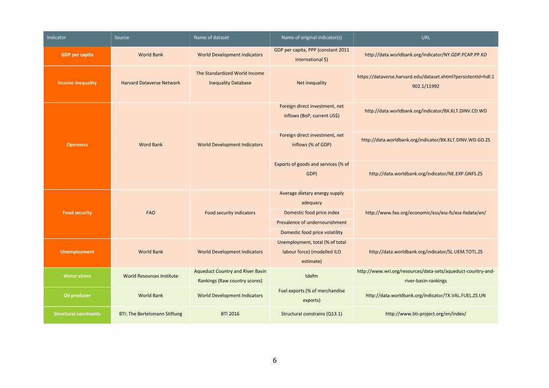
environmental factors, studied through 24 variables. The data used are extracted from

14 different datasets, which are all freely accessible by any user on the Internet. Table 2

provides details about the data provider, the dataset used, and the URL where on can

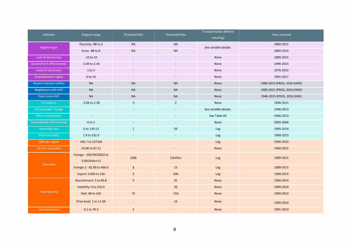
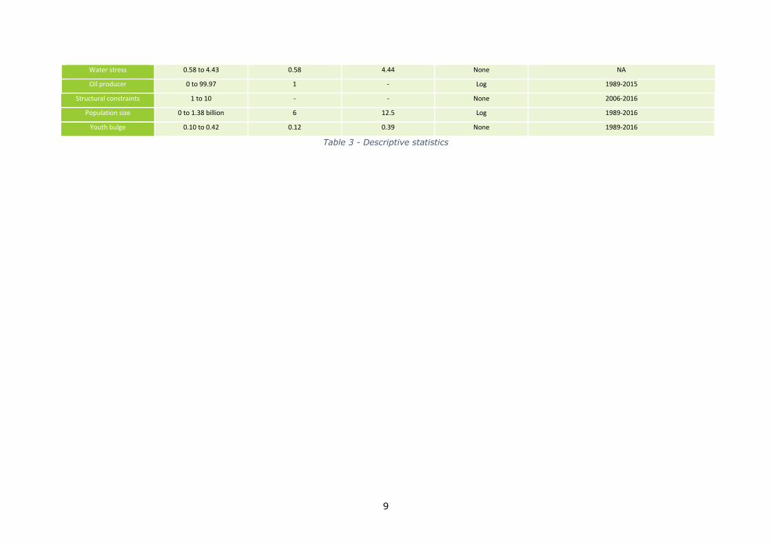
download the data. Table 3 presents some descriptive statistics: the original range of the

data distribution, the thresholds imposed, the transformation done and years covered by

each original dataset. While some of the datasets used are complete, others contain

3

missing data for specific years and/or specific countries. In order to overcome the lack of

data and be able to compute the model, the missing data are imputed (replacing missing

data with substituted values). In the imputation system adopted, data is taken from

either the closest known historical data (desk research is conducted for finding precise

information which would then justify the substituted value), or, if not possible, from

regional averages, or from similar countries. The imputation is included in the data

construction phase, making the data a single and complete dataset ready for statistical

analysis. For more information on the data management, please refer to the technical

report “Conflict Risk Indicators: Significance and Data Management in the GCRI” (doi.

10.2760/44005).

4

1 All datasets have been accessed on September 15th, 2017.

Table 1 - Variable sources (first part)1

Indicator Source Name of dataset Name of original indicator(s) URL

Regime type Center for Systemic Peace Polity IV Annual Time-Series,

1800-2015 PARCOM, EXREC http://www.systemicpeace.org/inscrdata.html

Lack of democracy Center for Systemic Peace Polity IV Annual Time-Series,

1800-2015 POLITY2 http://www.systemicpeace.org/inscrdata.html

Government effectiveness World Bank Government Effectiveness:

Estimate GE.EST

http://databank.worldbank.org/data/reports.aspx?source=worldwide-

governance-indicators

Level of repression Political Terror Scale Project PTS Data

Highest of the three indicators

in the set (PTS_A, PTS_H,

PTS_S)

http://www.politicalterrorscale.org/Data/Download.html

Empowerment rights CIRI Human Rights Data Project CIRI Data NEW_EMPINX http://www.humanrightsdata.com/p/data-documentation.html

Recent internal conflict HIIK; UCDP/PRIO

Battle related deaths, One-sided

violence, Non-state conflict,

Conflict Barometer 2016

Highest casualty estimates

http://ucdp.uu.se/downloads/

http://hiik.de/de/daten/ Neighbours with HVC HIIK; UCDP/PRIO

Battle related deaths, One-sided

violence, Non-state conflict,

Conflict Barometer 2016

Highest casualty estimates

Years since HVC HIIK; UCDP/PRIO Armed Conflict Dataset, Conflict

Barometer 2016 Conflicts of intensity level 2

Corruption World Bank Control of Corruption: Estimate CC.EST http://databank.worldbank.org/data/reports.aspx?source=worldwide-

governance-indicators

Ethnic Power Change ETH Zurich EPR Core Dataset Recording of dataset, see

variable page http://www.icr.ethz.ch/data/epr

5

Ethnic compilation ETH Zurich EPR Core Dataset Recording of dataset, see

variable page http://www.icr.ethz.ch/data/epr

Transnational ethnic bonds

CIDCM Center for International

Development &Conflict

Management

Marupdate_20042006 GC10 http://www.mar.umd.edu/mar_data.asp

Homicide rate World Bank World Development Indicators Intentional homicides (per

100,000 people) http://data.worldbank.org/indicator/VC.IHR.PSRC.P5

Infant mortality World Bank World Development Indicators Mortality rate, under-5 (per

1,000 live births) http://data.worldbank.org/indicator/SH.DYN.MORT

http://data.worldbank.org/indicator/SH.DYN.MORT

6

Indicator Source Name of dataset Name of original indicator(s) URL

GDP per capita World Bank World Development Indicators GDP per capita, PPP (constant 2011

international $) http://data.worldbank.org/indicator/NY.GDP.PCAP.PP.KD

Income inequality Harvard Dataverse Network

The Standardized World Income

Inequality Database

Net inequality https://dataverse.harvard.edu/dataset.xhtml?persistentId=hdl:1

902.1/11992

Openness Word Bank World Development Indicators

Foreign direct investment, net

inflows (BoP, current US$)

http://data.worldbank.org/indicator/BX.KLT.DINV.CD.WD

Foreign direct investment, net

inflows (% of GDP)

http://data.worldbank.org/indicator/BX.KLT.DINV.WD.GD.ZS

Exports of goods and services (% of

GDP)

http://data.worldbank.org/indicator/NE.EXP.GNFS.ZS

Food security FAO Food security indicators

Average dietary energy supply

adequacy

http://www.fao.org/economic/ess/ess-fs/ess-fadata/en/ Domestic food price index

Prevalence of undernourishment

Domestic food price volatility

Unemployment World Bank World Development Indicators

Unemployment, total (% of total

labour force) (modelled ILO

estimate)

http://data.worldbank.org/indicator/SL.UEM.TOTL.ZS

Water stress World Resources Institute Aqueduct Country and River Basin

Rankings (Raw country scores) tdefm

http://www.wri.org/resources/data-sets/aqueduct-country-and-

river-basin-rankings

Oil producer World Bank World Development Indicators Fuel exports (% of merchandise

exports) http://data.worldbank.org/indicator/TX.VAL.FUEL.ZS.UN

Structural constraints BTI: The Bertelsmann Stiftung BTI 2016 Structural constrains (Q13.1) http://www.bti-project.org/en/index/

7

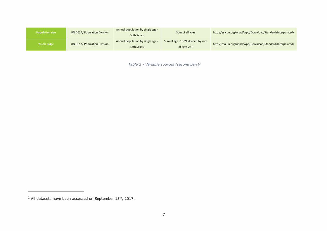
2 All datasets have been accessed on September 15th, 2017.

Population size UN DESA/ Population Division Annual population by single age -

Both Sexes. Sum of all ages http://esa.un.org/unpd/wpp/Download/Standard/Interpolated/

Youth bulge UN DESA/ Population Division Annual population by single age -

Both Sexes.

Sum of ages 15-24 divided by sum

of ages 25+ http://esa.un.org/unpd/wpp/Download/Standard/Interpolated/

Table 2 - Variable sources (second part)2

8

Indicator Original range Threshold Min Threshold Max Transformation (Before

rescaling) Years covered

Regime type Parcomp -88 to 5 NA NA

See variable details. 1800-2015

Exrec -88 to 8 NA NA 1800-2015

Lack of democracy -10 to 10 - - None 1800-2015

Government effectiveness -2.49 to 2.43 - - None 1996-2015

Level of repression 1 to 5 - - None 1976-2015

Empowerment rights 0 to 14 - - None 1981-2011

Recent internal conflict NA NA NA None 1989-2015 (PRIO), 2016 (HIIIK)

Neighbours with HVC NA NA NA None 1989-2015 (PRIO), 2016 (HIIIK)

Years since HVC NA NA NA None 1946-2015 (PRIO), 2016 (HIIK)

Corruption -2.06 to 2.58 -2 2 None 1996-2015

Ethnic power change - - - See variable details. 1946-2013

Ethnic compilation - - - See Table XX 1946-2013

Transnational ethnic bonds 0 to 3 - - None 2004-2006

Homicide rate 0 to 139.13 1 50 Log 1995-2014

Infant mortality 1.9 to 332.9 - - Log 1989-2015

GDP per capita 246.7 to 137164 - - Log 1990-2015

Income inequality 14.06 to 67.21 - - None 1960-2015

Openness

Foreign: -29679425810 to

3.065354e+12 100k 15billion Log 1989-2015

Foreign 2: -82.89 to 466.6 1 15 Log 1989-2015

Export: 0.005 to 230 3 200 Log 1989-2015

Food security

Nourishment: 5 to 80.8 5 35 None 1990-2014

Volatility: 0 to 210.4 - 20 None 1990-2014

Diet: 68 to 165 75 150 None 1990-2014

Price level: 1 to 11.69 - 10 None 1990-2014

Unemployment 0.1 to 39.3 2 - None 1991-2014

9

Water stress 0.58 to 4.43 0.58 4.44 None NA

Oil producer 0 to 99.97 1 - Log 1989-2015

Structural constraints 1 to 10 - - None 2006-2016

Population size 0 to 1.38 billion 6 12.5 Log 1989-2016

Youth bulge 0.10 to 0.42 0.12 0.39 None 1989-2016

Table 3 - Descriptive statistics

10

3. Regression model

Conflict studies use mostly regression analysis when they want to find a casual relation

between the risk of conflict and structural indicators (see e.g. Beck et al., 2000; Bennett

and Stam, 2000; Goldstone et al., 2000; Elbadawi and Sambanis, 2002). Based on

economic, social, environmental and political data, the regression model used for the

GCRI gives an insight into the probability and intensity of conflict at country level. The

present chapter describes the model and its outputs.

The regression models described in this chapter are the same generalized linear model

(glm) and linear model (lm) described in the two previous JRC technical reports on the

GCRI3, as well as for the model assumption, the dimension and the related notation.

The regression model is based on equations composed of the variables and respective

coefficients. This chapter contributes to the detailed description of the GCRI regression

model by explaining how the regression model operates (3.1), what the equations are

(3.2), and how the coefficients are calculated (3.3).

3.1. The three phases of the regression model

Figure 1 presents the three different phases that characterize the regression model.

Specific statistical methods, i.e. linear and logistic regression, are applied on the input

data in order to obtain the output in the form of 8 different scores.

3 “The Global Conflict Risk Index (GCRI) A Quantitative Model, Concept and Methodology” (2014),

and “The Global Conflict Risk Index (GCRI) Manual for data management and product output,

Version 5, Code documentation and methodology summary” (2016).

11

Figure 1 - The regression model

12

Phase 1 – Preparing the input data

The input data for the regression model are the 24 variables described in Table 1 and

Table 2 (p.4 and p.7). The preparation of the input data involves several steps. First of

all, the raw data are computed, by imputing data (if necessary) and rescaling the values

from 0 to 10 (the meaning of the rescaled values differs according to the variable4).

Once the first step of the preparation is completed, the second step can start, which

consist in further categorisations (Highly violent and violent conflicts; National and

subnational conflicts), as described below.

Type of conflict

Conflicts are categorized according to their type: High Violent Conflict (HVC) or Violent

Conflict (VC). This differentiation is made by applying threshold on the variable “Recent

Internal Conflict” whose values scale from 0 to 10 (no conflict to high violent conflict). A

conflict is classified in the “High Violent Conflict (HVC)” category, if the country/year

score for this specific variable is equal or higher than 8. On the other hand, a conflict is

classified in the “Violent Conflict (VC)” category when the threshold applied is of 5. Then

a lag5 is calculated, in order to analyse the change of the conflict situation in the next 4

years. More specifically, given a country/year, the highest value among the scores of the

4 following years is taken.

4 The meanings of the rescaled values are described in the technical report “Conflict Risk

Indicators: Significance and Data Management in the GCRI” (doi. 10.2760/44005).

5 A lag refers to a difference in time between an observation and a previous observation. (Eurostat

Statistics Explained, Glossary. Available at: http://ec.europa.eu/eurostat/statistics-

explained/index.php/Glossary:Lag. Retrieved on 26/07/2017)

Figure 2 - The regression model, Phase 1

http://ec.europa.eu/eurostat/statistics-explained/index.php/Glossary:Lag

http://ec.europa.eu/eurostat/statistics-explained/index.php/Glossary:Lag

13

Dimension

For each type of conflict (HVC and VC), we look at the two different dimensions of

conflict: national and subnational, based on the input data.

Dataset

As a result of the previous calculations, other variables are added into the dataset used:

- the lag of conflict intensity at the national level (based on the variable “Recent internal

conflict”);

- the lag of conflict intensity at the subnational level (based on the variable “Recent

internal conflict”);

- the maximum value between the intensity at the national and subnational levels

(based on the variable “Recent internal conflict”);

- the value of the variable “Neighbouring with HVC”;

- the value of the variable “Years since HVC”.

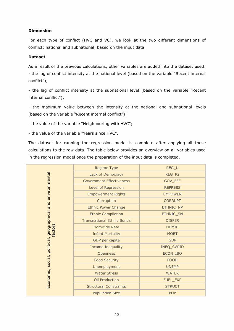
The dataset for running the regression model is complete after applying all these

calculations to the raw data. The table below provides an overview on all variables used

in the regression model once the preparation of the input data is completed.

Econom

ic,

socia

l, p

olitical, g

eogra

phic

al and e

nvironm

enta

l

facto

rs

Regime Type REG_U

Lack of Democracy REG_P2

Government Effectiveness GOV_EFF

Level of Repression REPRESS

Empowerment Rights EMPOWER

Corruption CORRUPT

Ethnic Power Change ETHNIC_NP

Ethnic Compilation ETHNIC_SN

Transnational Ethnic Bonds DISPER

Homicide Rate HOMIC

Infant Mortality MORT

GDP per capita GDP

Income Inequality INEQ_SWIID

Openness ECON_ISO

Food Security FOOD

Unemployment UNEMP

Water Stress WATER

Oil Production FUEL_EXP

Structural Constraints STRUCT

Population Size POP

14

Youth Bulge YOUTHBOTH

Maximum value between the intensity at

the national and subnational levels CON_INT

Value of the intensity in neighbouring

countries in HVC CON_NB

Value of years since HVC YRS_HVC

Intensity at the National level Intensity_Y_NP

Lag applied on the intensity at the

National level Intensity_Y4_NP

Intensity at the Subnational level Intensity_Y_SN

Lag applied on the intensity at the

Subnational level Intensity_Y4_SN

Applied

threshold of:

Boolean conditions

HVC

8 Intensity National

(Boolean) HVC_Y_NP

8 Lag of Intensity

National (Boolean) HVC_Y4_NP

8 Intensity Subnational

(Boolean) HVC_Y_SN

8 Lag of Intensity

Subnational (Boolean) HVC_Y4_SN

Boolean conditions

VC

5 Intensity National

(Boolean) VC_Y_NP

5 Lag of Intensity

National (Boolean) VC_Y4_NP

5 Intensity Subnational

(Boolean) VC_Y_SN

5 Lag of Intensity

Subnational (Boolean) VC_Y4_SN

Table 4 - Variables used in the regression model

Phase 2 – Defining the equations

Based on the two categorisations, HVC and VC, National and Subnational, the scope of

the assessment is therefore on the four cases listed below:

1) Probability and intensity of conflict in HVC at the subnational level;


15

2) Probability and intensity of conflict in HVC at the national level;

3) Probability and intensity of conflict in VC at the subnational level;

4) Probability and intensity of conflict in VC at the national level.

Two different equations are used to calculate the probability and the intensity, which

means that, for each of the four cases presented above, two equations are hence

needed. Therefore, 8 equations in total are required to assess the probability and

intensity of conflict, and describe the full conflict panorama.

- The intensity of a conflict is predicted using a linear model lm, which has the

following mathematical notation:

I = a0 + a1X1 + … + anXn

Where I is the intensity of the conflict, a0, a1, a2, .. an are the coefficients and X1,

X2, … Xn are the variables we consider in the model.

- The probability of a conflict is predicted using a logistic regression, which uses

the generalized linear model glm and is mathematically defined as follows:

Where p is the probability of a conflict, a0, a1, a2, .. an are the coefficients and X1,

X2, … Xn are the variables we consider in the model.

A schematic overview of the 8 equations, used to run the models, is presented in Table

5.

Name of the

equation

Type of conflict Dimension Probability or

Intensity

P_HVC_NP HVC NP PROBABILIY

P_HVC_SN HVC SN PROBABILIY

P_VC_NP VC NP PROBABILIY

P_VC_SN VC SN PROBABILIY

I_HVC_NP HVC NP INTENSITY

16

I_HVC_SN HVC SN INTENSITY

I_VC_NP VC NP INTENSITY

I_VC_SN VC SN INTENSITY

Table 5 - The eight equations of the regression model

Phase 3 – Getting the predictions

A “fitting” of the regression model is conducted so as to obtain the coefficients and

intercept of the equations. For this, we use the two models (glm and lm) that consist of

equations, while the quantities appearing in the equations are classified as variables. The

fitting uses selected series of data from 1989 to 2011, named the “Dataset for fitting”,

which was inherited from previous phase of development. In order to ensure

comparability throughout the years, this series is still being used. While all data from

1989 to 2011 are used for calculating the probability, a selection is made for calculating

the intensity. In fact, a filter is applied on the dataset (equal to 1, as presented in the

column “Filter” in the table below), in order to analyse only the cases experiencing a

conflict. The output of the process is a statistical set of information which includes the

coefficients and the intercept.

Name of the equation Filter Probability or Intensity

P_HVC_NP None PROBABILIY

P_HVC_SN None PROBABILIY


17

P_VC_NP None PROBABILIY

P_VC_SN None PROBABILIY

I_HVC_NP HVC_Y4_NP==1 INTENSITY

I_HVC_SN HVC_Y4_SN==1 INTENSITY

I_VC_NP VC_Y4_NP==1 INTENSITY

I_VC_SN VC_Y4_SN==1 INTENSITY

Table 6 - Filters applied on the dataset

The calculations to obtain the predictions are performed using the equations and the

coefficients and intercept obtained thanks to the “fitting” process. The outputs are scores

of the intensity and probability. The following sections describe in detail the equations

and the elements composing it.

3.2. Equations

All the 8 equations are composed of the same variables, except for ETHNIC_NP that is

used only for the National dimension and ETHNIC_SN that is used only for the

subnational one. We present in the sub-sections below the explicit equations and the

associated coefficients. As described in section 3.1 (p.10) on input data preparation,

conflicts are categorized according to their type (high violent conflict or violent conflict)

and dimension (national and subnational). The first sub-section describes the equations

associated with the conflict type “High Violent Conflict”, whereas the second sub-section

describes the equations associated with the conflict type “Violent Conflict”.

3.2.1. High Violent Model Equations

This sub-section introduces the equations for calculating the probability and intensity of

conflict, and the quantities appearing in the equations. In this sub-section, it applies

specifically to each of the two dimensions “National” and “Subnational”, inside the

conflict type “High Violent Conflict”. The quantities appearing in the equations presented

below are the variables (in black) and associated coefficients (in orange). The

coefficients are described in detailed in section 3.3 (p.20).

High Violent Conflict (HVC), National Dimension, Intensity (I_HVC_NP)

18

To calculate the Intensity for National Conflict (I_HVC_NP), the equation is:

I_HVC_NP = -1.108*REG_U+ -0.358*INEQ_SWIID+ -0.399*GDP_CAP+

0.203*REG_U*INEQ_SWIID+ 0.036*INEQ_SWIID*GDP_CAP+ 0.158*REG_U*GDP_CAP + -

0.029*REG_U*INEQ_SWIID*GDP_CAP+ 0.054*REG_P2+ -0.205*GOV_EFF+ -0.094*EMPOWER+

0.027*REPRESS+ 0.033*CON_NB+ -0.003*YRS_HVC+ 0.031*CON_INT+ -0.144 *MORT+ -0.036

*DISPER+ -0.101 *HOMIC+ -0.056 *ETHNIC_NP+ 0.185 *FOOD+ 0.059*POP+ -0.094*WATER+ -

0.051 *ECON_ISO+ 0.006 *FUEL_EXP+ 0.122*STRUCT+ -0.007*UNEMP+ 0.312*YOUTHBBOTH+

0.275*CORRUPT+ 9.574

High Violent Conflict (HVC), National Dimension, Probability (P_HVC_NP)

To calculate the Probability for National Conflicts (P_HVC_NP):

P_HVC_NP = EXP( ) / (1+EXP( ))

= -1.166*REG_U+ -1.685*INEQ_SWIID+ -1.302*GDP_CAP+ 0.219*REG_U*INEQ_SWIID+

0.181*INEQ_SWIID*GDP_CAP+ - 0.134*REG_U*GDP_CAP + -

0.026*REG_U*INEQ_SWIID*GDP_CAP + 0.024*REG_P2+ 0.310*GOV_EFF+ -0.105*EMPOWER+

0.152*REPRESS+ 0.069*CON_NB+ 0.171*YRS_HVC+ 0.229*CON_INT+ 0.214*MORT+ -

0.075*DISPER+ 0.104*HOMIC+ -0.037*ETHNIC_NP+ -0.089*FOOD+ 0.110*POP+

0.052*WATER+ 0.110*ECON_ISO+ 0.067*FUEL_EXP+ 0.448*STRUCT+ -0.098*UNEMP+

0.468*YOUTHBBOTH+ 0.034*CORRUPT+ -4.881

High Violent Conflict (HVC), Sub National Dimension, Intensity (I_HVC_SN)

To calculate the Intensity for Subnational Conflict (I_HVC_SN):

I_HVC_SN = -0.016*REG_U+ -0.132*INEQ_SWIID+ 0.078*GDP_CAP+

0.001*REG_U*INEQ_SWIID+ -0.006*INEQ_SWIID*GDP_CAP+ -0.009*REG_U*GDP_CAP+

0.002*REG_U*INEQ_SWIID*GDP_CAP + -0.006*REG_P2+ 0.039*GOV_EFF+ 0.022*EMPOWER+ -

0.009*REPRESS+ -0.008 *CON_NB+ 0.026*YRS_HVC+ -0.009*CON_INT+ 0.136*MORT+ -

0.041*DISPER+ 0.014*HOMIC+ 0.053*ETHNIC_SN+ 0.063*FOOD+ 0.056*POP+ 0.018*WATER+

-0.015*ECON_ISO+ 0.004*FUEL_EXP+ -0.128*STRUCT+ 0.052*UNEMP+ -0.043*YOUTHBBOTH+

0.037*CORRUPT+ 8.435

High Violent Conflict (HVC), Sub National Dimension, Probability (P_HVC_SN)

To calculate the Probability for Subnational Conflicts (P_HVC_SN):

P_HVC_SN = EXP( ) / (1+EXP( ))

19

= 1.010*REG_U+ 0.477*INEQ_SWIID+ 0.647*GDP_CAP+ -0.198*REG_U*INEQ_SWIID+ -

0.146*INEQ_SWIID*GDP_CAP+ - 0.194*REG_U*GDP_CAP +

0.038*REG_U*INEQ_SWIID*GDP_CAP + 0.008*REG_P2+ 0.439*GOV_EFF+ 0.06*EMPOWER+

0.221*REPRESS+ -0.008*CON_NB+ -0.050*YRS_HVC+ 0.308*CON_INT+ 0.281*MORT+ -

0.065*DISPER+ 0.147*HOMIC+ 0.257*ETHNIC_SN+ 0.062*FOOD+ 0.478*POP+ -

0.125*WATER+ -0.053*ECON_ISO+ -0.144*FUEL_EXP+ -0.221*STRUCT+ 0.241*UNEMP+ -

0.231*YOUTHBBOTH+ -0.139*CORRUPT+ -11.738

3.2.2. Violent Model Equations

This sub-section introduces the equations for calculating the probability and intensity of

conflict, and the quantities appearing in the equations. In this sub-section, it applies

specifically to each of the two dimensions “National” and “Subnational”, inside the

conflict type “Violent Conflict”. The quantities appearing in the equations presented

below are the variables (in black) and associated coefficients (in orange).

Violent Conflict (VC), National Dimension, Intensity (I_VC_NP)

To calculate the Intensity for National Conflict (I_VC_NP):

I_VC_NP = -1.238*REG_U+ -1.088*INEQ_SWIID+ -1.009*GDP_CAP+

0.189*REG_U*INEQ_SWIID+ 0.119*INEQ_SWIID*GDP_CAP+ 0.171*REG_U*GDP_CAP+ -

0.026*REG_U*INEQ_SWIID*GDP_CAP + 0.073*REG_P2+ -0.057*GOV_EFF+ -0.092*EMPOWER+

0.015*REPRESS+ -0.022*CON_NB+0.112*YRS_HVC+0.123*CON_INT+0.084*MORT+ -

0.032*DISPER+ 0.020*HOMIC+ -0.042*ETHNIC_NP+ -0.030*FOOD+ 0.024*POP+ -

0.140*WATER+ 0.015*ECON_ISO+ 0.065*FUEL_EXP+ 0.266*STRUCT+ -0.076*UNEMP+

0.330*YOUTHBBOTH+ 0.353*CORRUPT+8.331

Violent Conflict (VC), National Dimension, Probability (P_VC_NP)

To calculate the Probability for National Conflicts (P_VC_NP):

P_VC_NP = EXP( ) / (1+EXP( ))

= 0.324*REG_U+ -0.538*INEQ_SWIID+ -0.192*GDP_CAP+ 0.016*REG_U*INEQ_SWIID+


0.006*REG_U*INEQ_SWIID*GDP_CAP + -0.025*REG_P2+ 0.587*GOV_EFF+ -0.126*EMPOWER+

0.155*REPRESS+ 0.164*CON_NB+ 0.125*YRS_HVC+ 0.210*CON_INT+ 0.239*MORT+ -

0.075*DISPER+ 0.042*HOMIC+ -0.012*ETHNIC_NP+ -0.066*FOOD+ 0.181*POP+

0.211*WATER+ 0.003*ECON_ISO+ 0.053*FUEL_EXP+ 0.420*STRUCT+ 0.002*UNEMP+

0.196*YOUTHBBOTH+ -0.263*CORRUPT+ -10.06

20

Violent Conflict (VC), Sub National Dimension, Intensity (I_VC_SN)

To calculate the Intensity for Subnational Conflict (I_VC_SN):

I_VC_NP = 0.872*REG_U+ 0.446*INEQ_SWIID+ 0.777*GDP_CAP+ -

0.175*REG_U*INEQ_SWIID+ -0.110*INEQ_SWIID*GDP_CAP+ -0.157*REG_U*GDP_CAP+ 0.032

REG_U*INEQ_SWIID*GDP_CAP + 0.021*REG_P2+ 0.238*GOV_EFF+ 0.059*EMPOWER+

0.040*REPRESS+ -0.025*CON_NB+ 0.001*YRS_HVC+ 0.151*CON_INT+ -0.036*MORT+ -

0.057*DISPER+ 0.051*HOMIC+ 0.098*ETHNIC_SN+ -0.017*FOOD+ 0.310*POP+ -

0.075*WATER+ -0.070*ECON_ISO+ -0.075*FUEL_EXP+ -0.112*STRUCT+ 0.217*UNEMP+ -

0.160*YOUTHBBOTH+ 0.076*CORRUPT+0.275

Violent Conflict (VC), Sub National Dimension, Probability (P_VC_SN)

To calculate the Probability for Subnational Conflicts (P_VC_SN):

P_VC_SN = EXP( ) / (1+EXP( ))

= 1.074*REG_U+ 0.114*INEQ_SWIID+ -0.007*GDP_CAP+ -0.064*REG_U*INEQ_SWIID+ -


0.020*REG_U*INEQ_SWIID*GDP_CAP + -0.081*REG_P2+ 0.052*GOV_EFF+ -0.084*EMPOWER+

0.178*REPRESS+ -0.009*CON_NB+ -0.035*YRS_HVC+ 0.285*CON_INT+ 0.396*MORT+

0.072*DISPER+ 0.033*HOMIC+ 0.244*ETHNIC_SN+ 0.002*FOOD+ 0.289*POP+ 0.018*WATER+

-0.039*ECON_ISO+ 0.009*FUEL_EXP+ 0.025*STRUCT+ -0.100*UNEMP+ 0.091*YOUTHBBOTH+

0.164*CORRUPT+ -8.547

3.3. Coefficients

The coefficients give a specific weight to the variables they are associated to. The

coefficients are either positive (it corresponds to a reinforcing effect) or negative (it

corresponds to a hindering effect). As described in the section 3.2 (p.17) presenting the

equations, the coefficients are one of the two quantities appearing in the equations for

calculating the probability and intensity of conflict, together with the variables. The

following sub-sections list the coefficients used in the equations. The coefficients used for

the conflict type “High violent conflict” are presented in the first sub-section whereas the

coefficients used for the conflict type “Violent conflict” are presented in the second sub-

section.

21

3.3.1. High Violent Model Coefficients

This sub-section introduces the coefficients used for calculating the probability and

intensity of conflict. As shown in the tables below, the coefficients are associated to

specific variables. In this sub-section, it applies specifically to each of the two

dimensions “National” and “Subnational”, inside the conflict type “High Violent Conflict”.

High Violent Model Coefficients National Dimension

The coefficients used for calculating the probability of conflict are listed on the left side of

the tables (NP HVC Prob), and the coefficients used for calculating the intensity of

conflict are listed on the right side of the tables (NP HVC Intensity).

NP HVC Prob NP HVC Intensity

(Intercept) -4.8815 (Intercept) 9.5742

REG_U -1.1670 REG_U -1.1083

INEQ_SWIID -1.6856 INEQ_SWIID -0.3588

GDP_CAP -1.3024 GDP_CAP -0.3992

REG_P2 0.0246 REG_P2 0.0540

GOV_EFF 0.3109 GOV_EFF -0.2060

EMPOWER -0.1053 EMPOWER -0.0944

REPRESS 0.1526 REPRESS 0.0273

CON_NB 0.0694 CON_NB 0.0333

YRS_HVC 0.1717 YRS_HVC -0.0032

CON_INT 0.2291 CON_INT 0.0312

MORT 0.2148 MORT -0.1444

DISPER -0.0758 DISPER -0.0367

HOMIC 0.1047 HOMIC -0.1014

ETHNIC_NP -0.0374 ETHNIC_NP -0.0566

FOOD -0.0898 FOOD 0.1851

POP 0.1102 POP 0.0600

WATER 0.0530 WATER -0.0941

ECON_ISO 0.1108 ECON_ISO -0.0514

FUEL_EXP 0.0677 FUEL_EXP 0.0061

STRUCT 0.4485 STRUCT 0.1225

UNEMP -0.0985 UNEMP -0.0079

YOUTHBBOTH 0.4688 YOUTHBBOTH 0.3122

CORRUPT 0.0340 CORRUPT 0.2759

22

REG_U:INEQ_SWIID 0.2192 REG_U:INEQ_SWIID 0.2040

REG_U:GDP_CAP 0.1348 REG_U:GDP_CAP 0.1585

INEQ_SWIID:GDP_CAP 0.1818 INEQ_SWIID:GDP_CAP 0.0361

REG_U:INEQ_SWIID:GDP_CAP -0.0263 REG_U:INEQ_SWIID:GDP_CAP -0.0293

Table 7 - High Violent Model Coefficients National Dimension

High Violent Model Coefficients Sub National Dimension


the tables (SN HVC Prob), and the coefficients used for calculating the intensity of

conflict are listed on the right side of the tables (SN HVC Intensity).

SN HVC Prob SN HVC Intensity


REG_U 1.0105 REG_U -0.0168

INEQ_SWIID 0.4779 INEQ_SWIID -0.1322

GDP_CAP 0.6470 GDP_CAP 0.0788

REG_P2 0.0081 REG_P2 -0.0063

GOV_EFF 0.4392 GOV_EFF 0.0392

EMPOWER 0.0620 EMPOWER 0.0226

REPRESS 0.2214 REPRESS -0.0097

CON_NB -0.0088 CON_NB -0.0089

YRS_HVC -0.0509 YRS_HVC 0.0262

CON_INT 0.3080 CON_INT -0.0091

MORT 0.2813 MORT 0.1364


HOMIC 0.1479 HOMIC 0.0145

ETHNIC_SN 0.2573 ETHNIC_SN 0.0538

FOOD 0.0621 FOOD 0.0635

POP 0.4784 POP 0.0569

WATER -0.1255 WATER 0.0181

ECON_ISO -0.0532 ECON_ISO -0.0155

FUEL_EXP -0.1443 FUEL_EXP 0.0048

STRUCT -0.2211 STRUCT -0.1288

UNEMP 0.2417 UNEMP 0.0522

YOUTHBBOTH -0.2312 YOUTHBBOTH -0.0435

CORRUPT -0.1391 CORRUPT 0.0372

23

REG_U:INEQ_SWIID -0.1987 REG_U:INEQ_SWIID 0.0014

REG_U:GDP_CAP -0.1950 REG_U:GDP_CAP -0.0092

INEQ_SWIID:GDP_CAP -0.1463 INEQ_SWIID:GDP_CAP -0.0067

REG_U:INEQ_SWIID:GDP_CAP 0.0387 REG_U:INEQ_SWIID:GDP_CAP 0.0028

Table 8 - High Violent Model Coefficients Sub National Dimension

3.3.2. Violent Model Coefficients

This sub-section introduces the coefficients used for calculating the probability and

intensity of conflict. As shown in the tables below, the coefficients are associated to

specific variables. In this sub-section, it applies specifically to each of the two

dimensions “National” and “Subnational”, inside the conflict type “Violent Conflict”.

Violent Model Coefficients National Dimension


the tables (NP VC Prob), and the coefficients used for calculating the intensity of conflict

are listed on the right side of the tables (NP VC Intensity).

NP VC Prob NP VC Intensity


REG_U 0.3250 REG_U -1.2381

INEQ_SWIID -0.5386 INEQ_SWIID -1.0888

GDP_CAP -0.1929 GDP_CAP -1.0095

REG_P2 -0.0250 REG_P2 0.0734

GOV_EFF 0.5877 GOV_EFF -0.0577

EMPOWER -0.1265 EMPOWER -0.0924


CON_NB 0.1640 CON_NB -0.0225

YRS_HVC 0.1257 YRS_HVC 0.1126


MORT 0.2400 MORT 0.0841



ETHNIC_NP -0.0126 ETHNIC_NP -0.0426

FOOD -0.0661 FOOD -0.0301

POP 0.1814 POP 0.0250

24

WATER 0.2120 WATER -0.1402

ECON_ISO 0.0039 ECON_ISO 0.0160

FUEL_EXP 0.0530 FUEL_EXP 0.0656

STRUCT 0.4203 STRUCT 0.2664

UNEMP 0.0029 UNEMP -0.0763

YOUTHBBOTH 0.1969 YOUTHBBOTH 0.3305

CORRUPT -0.2631 CORRUPT 0.3531

REG_U:INEQ_SWIID 0.0166 REG_U:INEQ_SWIID 0.1891

REG_U:GDP_CAP -0.0930 REG_U:GDP_CAP 0.1718

INEQ_SWIID:GDP_CAP 0.0280 INEQ_SWIID:GDP_CAP 0.1199

REG_U:INEQ_SWIID:GDP_CAP 0.0063 REG_U:INEQ_SWIID:GDP_CAP -0.0269

Table 9 - Violent Model Coefficients National Dimension

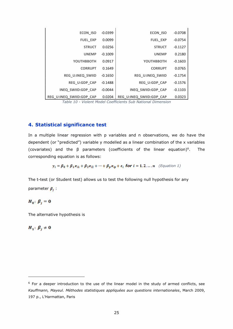
Violent Model Coefficients Sub National Dimension


the tables (SN VC Prob), and the coefficients used for calculating the intensity of conflict

are listed on the right side of the tables (SN VC Intensity).

SN VC Prob SN VC Intensity


REG_U 1.0750 REG_U 0.8728

INEQ_SWIID 0.1146 INEQ_SWIID 0.4468

GDP_CAP -0.0076 GDP_CAP 0.7776

REG_P2 -0.0814 REG_P2 0.0214

GOV_EFF -0.0523 GOV_EFF 0.2382

EMPOWER -0.0846 EMPOWER 0.0595


CON_NB -0.0091 CON_NB -0.0251

YRS_HVC -0.0356 YRS_HVC 0.0016


MORT 0.3964 MORT -0.0362

DISPER 0.0722 DISPER -0.0572


ETHNIC_SN 0.2446 ETHNIC_SN 0.0985

FOOD 0.0027 FOOD -0.0178

POP 0.2896 POP 0.3101

WATER 0.0187 WATER -0.0751

25

ECON_ISO -0.0399 ECON_ISO -0.0708

FUEL_EXP 0.0099 FUEL_EXP -0.0754

STRUCT 0.0256 STRUCT -0.1127

UNEMP -0.1009 UNEMP 0.2180

YOUTHBBOTH 0.0917 YOUTHBBOTH -0.1603

CORRUPT 0.1649 CORRUPT 0.0765

REG_U:INEQ_SWIID -0.1650 REG_U:INEQ_SWIID -0.1754

REG_U:GDP_CAP -0.1488 REG_U:GDP_CAP -0.1576

INEQ_SWIID:GDP_CAP -0.0044 INEQ_SWIID:GDP_CAP -0.1103

REG_U:INEQ_SWIID:GDP_CAP 0.0204 REG_U:INEQ_SWIID:GDP_CAP 0.0323

Table 10 - Violent Model Coefficients Sub National Dimension

4. Statistical significance test

In a multiple linear regression with p variables and n observations, we do have the

dependent (or “predicted”) variable y modelled as a linear combination of the x variables

(covariates) and the β parameters (coefficients of the linear equation)6. The

corresponding equation is as follows:

(Equation 1)

The t-test (or Student test) allows us to test the following null hypothesis for any

parameter :

The alternative hypothesis is

6 For a deeper introduction to the use of the linear model in the study of armed conflicts, see

Kauffmann, Mayeul. Méthodes statistiques appliquées aux questions internationales, March 2009,

197 p., L’Harmattan, Paris

26

The null hypothesis is the hypothesis that the coefficient equals zero. The ability to

assess this hypothesis and the alternative hypothesis contributes to the model’s

falsifiability and is a significant element of the scientificity of the approach7.

It should be noted here that we do not know the true value of the coefficient

(because of, inter alia, measurement errors); we only have an estimate of the jth

coefficient of equation (Equation 1).

The estimates are reported in the first numeric column of the tables showing the

estimated models below; the first row (“Intercept”) corresponds to (the constant

part of the equation), while the following rows correspond to the coefficients relevant

to each covariate .

Small random variations in the dataset may lead to an estimate of the coefficient

which is slightly different from zero, but not significantly different enough to allow us

to reject the null hypothesis that the true (unknown) coefficient is indeed zero ; in

this case, this is equivalent to saying that the covariate has no significant impact on

(in our case, that a given GCRI component has no significant impact on the intensity

of conflict in a particular model, assuming that this model is appropriate). If is

rejected, we then keep the alternative hypothesis that the parameter is most likely

different from zero.

In the case of the linear models used to model the intensity of conflict, the test statistic

is the t statistic, defined as the estimate of the parameter divided by its standard

deviation (this is shown in tables below in the column “t value”). Under appropriate

hypotheses, the test statistic t follows a Student’s distribution with n - (p+1) degrees of

freedom. If there was no uncertainty and if the covariates had no impact on y, then the t

7 For a more thorough discussion of these concepts in view of Popper’s epistemology, see

Kauffmann, Mayeul, “Introduction” in Kauffmann, Mayeul (ed.) Building and Using Datasets on

Armed Conflicts, May 2008, Amsterdam: IOS Press, 204 p. ISBN: 978-1586038472

http://ebooks.iospress.nl/volume/building-and-using-datasets-on-armed-conflicts


27

values would all be equal to zero. Because of uncertainty, a t value different from zero

might still be compatible with the null hypothesis. The last column of the table, Pr(>|t|),

also named the “p-value”, measures the probability that we get a t value that far from

zero (or even further from zero than the t value), given that the null hypothesis is

assumed to be true. If this probability is very low (often, below 5% or 0.05) we use a

decision rule which says that the null hypothesis should be rejected. If the p-value is

higher than the threshold, then the null hypothesis cannot be rejected.

It should be emphasised that the p-value associated with the t-test is only a hint on the

likelihood of the impact of a covariate on the dependent variable. In no way can a p-

value of 0.05 be interpreted as: “the probability of incorrectly rejecting a true null

hypothesis is 5 %” (such a probability has been measured to be greater than 23 % and

typically close to 50 % by Sellke et al. (2001))8 .

The interpretation of the four logistic models9 below (modelling the probability of

conflict) is similar to that of the linear models (for conflict intensity) if we look at the p-

value. The test statistic, however, is different. In effect, it can be demonstrated that the

estimate divided by its standard errors follows (under the null hypothesis) a normal

distribution (not a Student distribution); in this case, the test statistic is named z.

Hence, the p-value is Pr(>|z|) as shown in the last column of the tables related to the

logistic models.

Probability of VC_NP logistic model

Estimate Std. Error z value Pr(>|z|)

8 Thomas SELLKE, M. J. BAYARRI, and James O. BERGER, “Calibration of p Values for Testing

Precise Null Hypotheses”, The American Statistician, February 2001, Vol. 55, No. 1, pp. 63-64.

Available at http://www.cems.uvm.edu/~jbuzas/buzas/calibrating_p_values.pdf

9 For a presentation of the Generalized Linear Model (of which the logistic model is a particular

case) in the context of conflict modelling, and a review of several GLMs, see: Kauffmann, Mayeul,

“Short Term and Event Interdependence Matter: A Political Economy Continuous Model of Civil

War”, in Peace Economics, Peace Science and Public Policy, Vol. 13, Issue 1, 2007, BE-Press

(Berkeley), 19 p. See also: Kucera Jan; Kauffmann Mayeul; Duta Ana-Maria; Soler Ivette Tarrida;

Tenerelli Patrizia; Trianni Giovanna; Hale Catherine; Rizzo Lauren; Ferri Stefano. Armed conflicts

and natural resources - Scientific report on Global Atlas and Information Centre for Conflicts and

Natural Resources. 2011. European Commission - Scientific and Technical Research Reports. ISBN

978-92-79-20498-2, pp. 23-28. Kauffmann, Mayeul, Gouvernance économique mondiale et

conflits armés. Banque mondiale, FMI et GATT-OMC, Paris: l’Harmattan, May 2006, 330 p.

http://www.cems.uvm.edu/~jbuzas/buzas/calibrating_p_values.pdf

28

(Intercept) -10.0602 2.2051 -4.56 0.0000

REG_U 0.3250 0.3691 0.88 0.3787

INEQ_SWIID -0.5386 0.3885 -1.39 0.1656

GDP_CAP -0.1929 0.3489 -0.55 0.5804

REG_P2 -0.0250 0.0359 -0.70 0.4869

GOV_EFF 0.5877 0.1122 5.24 0.0000

EMPOWER -0.1265 0.0419 -3.02 0.0026

REPRESS 0.1550 0.0387 4.01 0.0001

CON_NB 0.1640 0.0200 8.22 0.0000

YRS_HVC 0.1257 0.0235 5.34 0.0000

CON_INT 0.2106 0.0245 8.61 0.0000

MORT 0.2400 0.0838 2.86 0.0042

DISPER -0.0759 0.0192 -3.95 0.0001

HOMIC 0.0424 0.0355 1.19 0.2333

ETHNIC_NP -0.0126 0.0350 -0.36 0.7180

FOOD -0.0661 0.0443 -1.49 0.1355

POP 0.1814 0.0430 4.22 0.0000

WATER 0.2120 0.0427 4.97 0.0000

ECON_ISO 0.0039 0.0565 0.07 0.9452

FUEL_EXP 0.0530 0.0229 2.31 0.0207

STRUCT 0.4203 0.0607 6.92 0.0000

UNEMP 0.0029 0.0360 0.08 0.9348

29

YOUTHBBOTH 0.1969 0.0665 2.96 0.0031

CORRUPT -0.2631 0.0965 -2.73 0.0064

REG_U:INEQ_SWIID 0.0166 0.0678 0.25 0.8060

REG_U:GDP_CAP -0.0930 0.0577 -1.61 0.1068

INEQ_SWIID:GDP_CAP 0.0280 0.0631 0.44 0.6572

REG_U:INEQ_SWIID:GDP_CAP 0.0063 0.0107 0.59 0.5557

Table 11- Probability of VC_NP logistic model

Intensity of VC_NP linear model

Estimate Std. Error t value Pr(>|t|)

(Intercept) 8.3311 2.9236 2.85 0.0045

REG_U -1.2381 0.4856 -2.55 0.0110

INEQ_SWIID -1.0888 0.5332 -2.04 0.0416

GDP_CAP -1.0095 0.4492 -2.25 0.0250

REG_P2 0.0734 0.0491 1.49 0.1355

GOV_EFF -0.0577 0.1540 -0.37 0.7082

EMPOWER -0.0924 0.0527 -1.75 0.0801

REPRESS 0.0159 0.0527 0.30 0.7634

CON_NB -0.0225 0.0281 -0.80 0.4237

YRS_HVC 0.1126 0.0273 4.12 0.0000

CON_INT 0.1238 0.0322 3.84 0.0001

MORT 0.0841 0.1207 0.70 0.4861

DISPER -0.0323 0.0254 -1.27 0.2033

30

HOMIC 0.0203 0.0533 0.38 0.7030

ETHNIC_NP -0.0426 0.0402 -1.06 0.2895

FOOD -0.0301 0.0714 -0.42 0.6737

POP 0.0250 0.0691 0.36 0.7177

WATER -0.1402 0.0588 -2.38 0.0175

ECON_ISO 0.0160 0.0747 0.21 0.8309

FUEL_EXP 0.0656 0.0315 2.08 0.0375

STRUCT 0.2664 0.0849 3.14 0.0018

UNEMP -0.0763 0.0530 -1.44 0.1501

YOUTHBBOTH 0.3305 0.1016 3.25 0.0012

CORRUPT 0.3531 0.1336 2.64 0.0085

REG_U:INEQ_SWIID 0.1891 0.0867 2.18 0.0295

REG_U:GDP_CAP 0.1718 0.0731 2.35 0.0190


REG_U:INEQ_SWIID:GDP_CAP -0.0269 0.0134 -2.01 0.0445

Table 12 – Intensity of VC_NP linear model

Probability of VC_SN logistic model


(Intercept) -8.5473 1.4543 -5.88 0.0000

REG_U 1.0750 0.2613 4.11 0.0000

INEQ_SWIID 0.1146 0.2829 0.41 0.6853

GDP_CAP -0.0076 0.2598 -0.03 0.9765

31

REG_P2 -0.0814 0.0327 -2.49 0.0128

GOV_EFF -0.0523 0.0973 -0.54 0.5910

EMPOWER -0.0846 0.0369 -2.29 0.0221

REPRESS 0.1784 0.0345 5.18 0.0000

CON_NB -0.0091 0.0159 -0.58 0.5645

YRS_HVC -0.0356 0.0244 -1.45 0.1457

CON_INT 0.2855 0.0232 12.33 0.0000

MORT 0.3964 0.0777 5.10 0.0000

DISPER 0.0722 0.0168 4.30 0.0000

HOMIC 0.0340 0.0312 1.09 0.2755

ETHNIC_SN 0.2446 0.0258 9.48 0.0000

FOOD 0.0027 0.0422 0.06 0.9497

POP 0.2896 0.0353 8.20 0.0000

WATER 0.0187 0.0371 0.50 0.6151

ECON_ISO -0.0399 0.0505 -0.79 0.4288

FUEL_EXP 0.0099 0.0201 0.50 0.6204

STRUCT 0.0256 0.0498 0.51 0.6070

UNEMP -0.1009 0.0284 -3.55 0.0004

YOUTHBBOTH 0.0917 0.0533 1.72 0.0852

CORRUPT 0.1649 0.0854 1.93 0.0535

REG_U:INEQ_SWIID -0.1650 0.0527 -3.13 0.0017

REG_U:GDP_CAP -0.1488 0.0451 -3.30 0.0010

32

INEQ_SWIID:GDP_CAP -0.0044 0.0488 -0.09 0.9276


Table 13 – Probability of VC_SN logistic model

Intensity of VC_SN linear model


(Intercept) 0.2752 1.5629 0.18 0.8603

REG_U 0.8728 0.2510 3.48 0.0005

INEQ_SWIID 0.4468 0.3077 1.45 0.1469

GDP_CAP 0.7776 0.2668 2.91 0.0036

REG_P2 0.0214 0.0338 0.63 0.5277

GOV_EFF 0.2382 0.1071 2.22 0.0264

EMPOWER 0.0595 0.0371 1.61 0.1084

REPRESS 0.0407 0.0382 1.06 0.2879

CON_NB -0.0251 0.0175 -1.44 0.1513

YRS_HVC 0.0016 0.0190 0.08 0.9332

CON_INT 0.1519 0.0208 7.29 0.0000

MORT -0.0362 0.0793 -0.46 0.6483

DISPER -0.0572 0.0188 -3.04 0.0024

HOMIC 0.0512 0.0366 1.40 0.1626

ETHNIC_SN 0.0985 0.0258 3.82 0.0001

FOOD -0.0178 0.0441 -0.40 0.6871

POP 0.3101 0.0393 7.88 0.0000

33

WATER -0.0751 0.0421 -1.78 0.0749

ECON_ISO -0.0708 0.0540 -1.31 0.1901

FUEL_EXP -0.0754 0.0216 -3.49 0.0005

STRUCT -0.1127 0.0573 -1.97 0.0494

UNEMP 0.2180 0.0361 6.03 0.0000

YOUTHBBOTH -0.1603 0.0638 -2.51 0.0122

CORRUPT 0.0765 0.1007 0.76 0.4479

REG_U:INEQ_SWIID -0.1754 0.0505 -3.48 0.0005

REG_U:GDP_CAP -0.1576 0.0396 -3.98 0.0001



Table 14 –Intensity of VC_SN linear model

Probability of HVC_NP logistic model


(Intercept) -4.8815 2.8445 -1.72 0.0861

REG_U -1.1670 0.5321 -2.19 0.0283

INEQ_SWIID -1.6856 0.5443 -3.10 0.0020

GDP_CAP -1.3024 0.4818 -2.70 0.0069

REG_P2 0.0246 0.0481 0.51 0.6090

GOV_EFF 0.3109 0.1579 1.97 0.0490

EMPOWER -0.1053 0.0557 -1.89 0.0589

REPRESS 0.1526 0.0526 2.90 0.0037

34

CON_NB 0.0694 0.0264 2.63 0.0087

YRS_HVC 0.1717 0.0261 6.58 0.0000

CON_INT 0.2291 0.0319 7.19 0.0000

MORT 0.2148 0.1111 1.93 0.0533

DISPER -0.0758 0.0261 -2.90 0.0037

HOMIC 0.1047 0.0519 2.02 0.0436

ETHNIC_NP -0.0374 0.0413 -0.91 0.3645

FOOD -0.0898 0.0652 -1.38 0.1683

POP 0.1102 0.0621 1.77 0.0761

WATER 0.0530 0.0614 0.86 0.3880

ECON_ISO 0.1108 0.0748 1.48 0.1387

FUEL_EXP 0.0677 0.0312 2.17 0.0297

STRUCT 0.4485 0.0833 5.39 0.0000

UNEMP -0.0985 0.0531 -1.85 0.0636

YOUTHBBOTH 0.4688 0.0955 4.91 0.0000

CORRUPT 0.0340 0.1424 0.24 0.8111

REG_U:INEQ_SWIID 0.2192 0.0936 2.34 0.0192

REG_U:GDP_CAP 0.1348 0.0796 1.69 0.0902



Table 15 – Probability of HVC_NP logistic model

Intensity of HVC_NP linear model

35


(Intercept) 9.5742 1.6529 5.79 0.0000

REG_U -1.1083 0.3092 -3.58 0.0004

INEQ_SWIID -0.3588 0.3001 -1.20 0.2327

GDP_CAP -0.3992 0.2596 -1.54 0.1251

REG_P2 0.0540 0.0279 1.93 0.0540

GOV_EFF -0.2060 0.0955 -2.16 0.0319

EMPOWER -0.0944 0.0291 -3.25 0.0013

REPRESS 0.0273 0.0316 0.87 0.3874

CON_NB 0.0333 0.0148 2.24 0.0257

YRS_HVC -0.0032 0.0143 -0.23 0.8217

CON_INT 0.0312 0.0179 1.74 0.0823

MORT -0.1444 0.0737 -1.96 0.0512

DISPER -0.0367 0.0160 -2.30 0.0223

HOMIC -0.1014 0.0396 -2.56 0.0110

ETHNIC_NP -0.0566 0.0192 -2.95 0.0034

FOOD 0.1851 0.0449 4.12 0.0000

POP 0.0600 0.0420 1.43 0.1547

WATER -0.0941 0.0415 -2.27 0.0241

ECON_ISO -0.0514 0.0430 -1.20 0.2327

FUEL_EXP 0.0061 0.0172 0.35 0.7239

STRUCT 0.1225 0.0514 2.38 0.0179

36

UNEMP -0.0079 0.0329 -0.24 0.8097

YOUTHBBOTH 0.3122 0.0695 4.49 0.0000

CORRUPT 0.2759 0.1055 2.62 0.0094

REG_U:INEQ_SWIID 0.2040 0.0524 3.89 0.0001

REG_U:GDP_CAP 0.1585 0.0441 3.60 0.0004



Table 16 – Intensity of HVC_NP linear model

Probability of HVC_SN logistic model


(Intercept) -8.5473 1.4543 -5.88 0.0000

REG_U 1.0750 0.2613 4.11 0.0000

INEQ_SWIID 0.1146 0.2829 0.41 0.6853

GDP_CAP -0.0076 0.2598 -0.03 0.9765

REG_P2 -0.0814 0.0327 -2.49 0.0128

GOV_EFF -0.0523 0.0973 -0.54 0.5910

EMPOWER -0.0846 0.0369 -2.29 0.0221

REPRESS 0.1784 0.0345 5.18 0.0000

CON_NB -0.0091 0.0159 -0.58 0.5645

YRS_HVC -0.0356 0.0244 -1.45 0.1457

CON_INT 0.2855 0.0232 12.33 0.0000

MORT 0.3964 0.0777 5.10 0.0000

37

DISPER 0.0722 0.0168 4.30 0.0000

HOMIC 0.0340 0.0312 1.09 0.2755

ETHNIC_SN 0.2446 0.0258 9.48 0.0000

FOOD 0.0027 0.0422 0.06 0.9497

POP 0.2896 0.0353 8.20 0.0000

WATER 0.0187 0.0371 0.50 0.6151

ECON_ISO -0.0399 0.0505 -0.79 0.4288

FUEL_EXP 0.0099 0.0201 0.50 0.6204

STRUCT 0.0256 0.0498 0.51 0.6070

UNEMP -0.1009 0.0284 -3.55 0.0004

YOUTHBBOTH 0.0917 0.0533 1.72 0.0852

CORRUPT 0.1649 0.0854 1.93 0.0535

REG_U:INEQ_SWIID -0.1650 0.0527 -3.13 0.0017

REG_U:GDP_CAP -0.1488 0.0451 -3.30 0.0010



Table 17 – Probability of HVC_SN logistic model

Intensity of HVC_SN linear model


(Intercept) 0.2752 1.5629 0.18 0.8603

REG_U 0.8728 0.2510 3.48 0.0005

INEQ_SWIID 0.4468 0.3077 1.45 0.1469

38

GDP_CAP 0.7776 0.2668 2.91 0.0036

REG_P2 0.0214 0.0338 0.63 0.5277

GOV_EFF 0.2382 0.1071 2.22 0.0264

EMPOWER 0.0595 0.0371 1.61 0.1084

REPRESS 0.0407 0.0382 1.06 0.2879

CON_NB -0.0251 0.0175 -1.44 0.1513

YRS_HVC 0.0016 0.0190 0.08 0.9332

CON_INT 0.1519 0.0208 7.29 0.0000

MORT -0.0362 0.0793 -0.46 0.6483

DISPER -0.0572 0.0188 -3.04 0.0024

HOMIC 0.0512 0.0366 1.40 0.1626

ETHNIC_SN 0.0985 0.0258 3.82 0.0001

FOOD -0.0178 0.0441 -0.40 0.6871

POP 0.3101 0.0393 7.88 0.0000

WATER -0.0751 0.0421 -1.78 0.0749

ECON_ISO -0.0708 0.0540 -1.31 0.1901

FUEL_EXP -0.0754 0.0216 -3.49 0.0005

STRUCT -0.1127 0.0573 -1.97 0.0494

UNEMP 0.2180 0.0361 6.03 0.0000

YOUTHBBOTH -0.1603 0.0638 -2.51 0.0122

CORRUPT 0.0765 0.1007 0.76 0.4479

REG_U:INEQ_SWIID -0.1754 0.0505 -3.48 0.0005

39

REG_U:GDP_CAP -0.1576 0.0396 -3.98 0.0001



Table 18 – Intensity of HVC_SN linear model

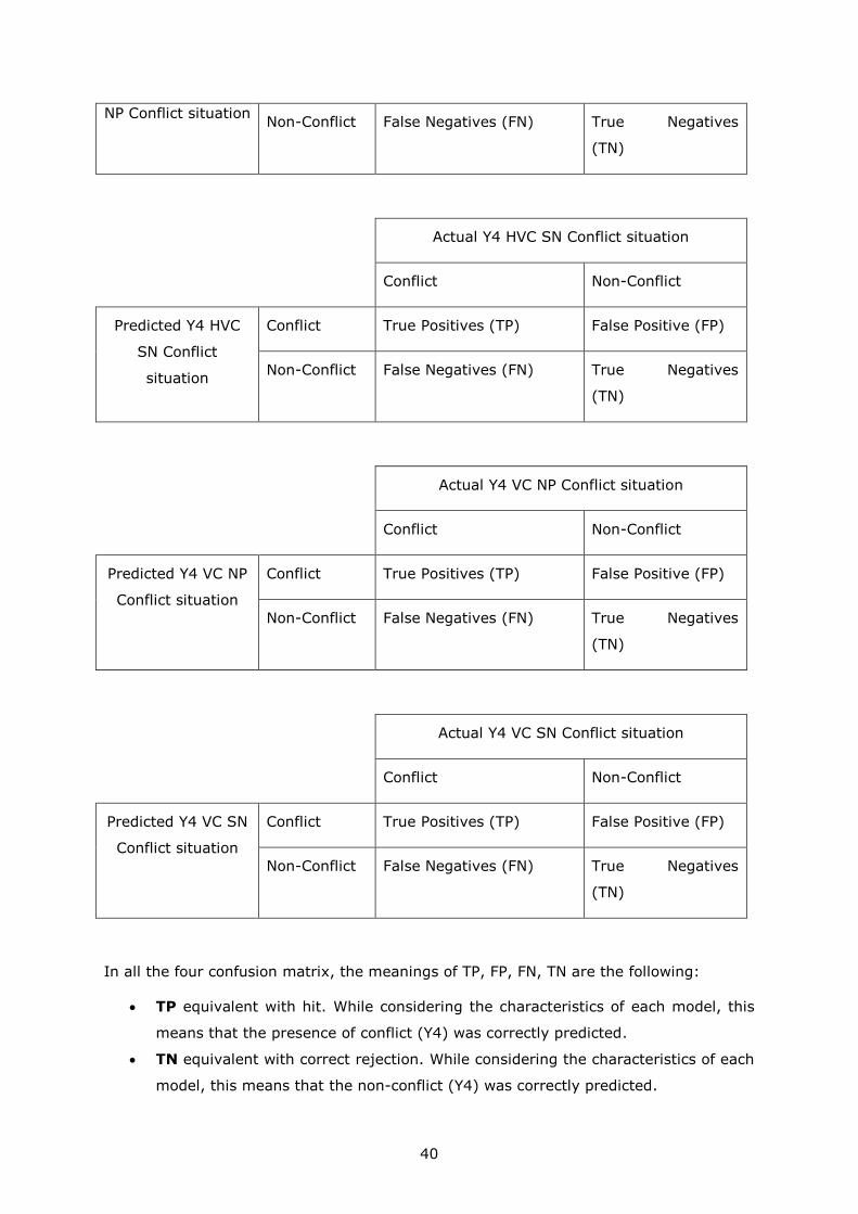
5. Statistical Metrics

In predictive analytics, a table of confusion (also called a confusion matrix) is a table

with two rows and two columns that reports the number of false positives, false

negatives, true positives and true negatives. This allows more detailed analysis than

mere proportion of correct classifications (accuracy). Accuracy is not a reliable metric for

the real performance of a classifier, because it will yield misleading results if the data set

is unbalanced (that is, when the numbers of observations in different classes vary

greatly).

Assuming the confusion matrix mentioned above, its corresponding table of confusion

would be for the conflict class:

Actual Y4 Conflict situation

Conflict Non-Conflict

Predicted Y4

Conflict situation

Conflict True Positives (TP) False Positive (FP)

Non-Conflict False Negatives (FN) True Negatives

(TN)

However, since we have 2 models (HVC/VC) in 2 dimensions (NP/SN), we obtain in total

4 confusion matrix, as shown in the tables below.

Actual Y4 HVC NP Conflict situation


Predicted Y4 HVC Conflict True Positives (TP) False Positive (FP)

40

NP Conflict situation Non-Conflict False Negatives (FN) True Negatives

(TN)

Actual Y4 HVC SN Conflict situation


Predicted Y4 HVC

SN Conflict

situation



(TN)

Actual Y4 VC NP Conflict situation


Predicted Y4 VC NP

Conflict situation



(TN)

Actual Y4 VC SN Conflict situation


Predicted Y4 VC SN

Conflict situation



(TN)

In all the four confusion matrix, the meanings of TP, FP, FN, TN are the following:

TP equivalent with hit. While considering the characteristics of each model, this

means that the presence of conflict (Y4) was correctly predicted.

TN equivalent with correct rejection. While considering the characteristics of each

model, this means that the non-conflict (Y4) was correctly predicted.

41

FP equivalent with false alarm. While considering the characteristics of each

model, this means that the conflict (Y4) was not correctly predicted; the conflict

did not occur.

FN equivalent with miss. While considering the characteristics of each model, this

means that the conflict (Y4) was not correctly predicted; the conflict occurred,

although it was not predicted.

There are in addition the totals of Actual/real (Y4) situations/cases:

P condition positive. The number of real positive cases in the data.

N condition negatives. The number of real negative cases in the data.

Terminology and derivations from a confusion matrix

Sensitivity, recall, hit rate or true positive rate (TPR) measures the proportion of

positives that are correctly identified:

Specificity or true negative rate (TNR) measures the proportion of negatives that are

correctly identified:

Precision or positive predictive value (PPV) is the fraction of relevant positives

instances among the retrieved instances:

Negative predictive value (NPV) is the fraction of relevant negatives instances among

the retrieved instances:

Fall-out or false positive rate (FPR) is calculated as the ratio between the number of

negative events wrongly categorized as positive (false positives) and the total number of

actual negative events (regardless of classification):

42

Complementarily, the Miss rate or false negative rate (FNR) is the proportion of positives

which yield negative test outcomes with the test, i.e. the conditional probability of a

negative test result given that the condition being looked for is present.

Accuracy (ACC) has two definitions:

1. More commonly, it is a description of systematic errors, a measure of statistical

bias; as these cause a difference between a result and a "true" value,

International Organization for Standardization (ISO) calls this trueness.

2. Alternatively, ISO defines accuracy as describing a combination of both types of

observational error above (random and systematic), so high accuracy requires

both high precision and high trueness.

In simplest terms, given a set of data points from a series of measurements, the set can

be said to be precise if the values are close to the average value of the quantity being

measured, while the set can be said to be accurate if the values are close to the true

value of the quantity being measured. The two concepts are independent of each other,

so a particular set of data can be said to be either accurate, or precise, or both, or

neither.

Following a more commonly used definition in the fields of science and engineering, the

accuracy of a measurement system is the degree of closeness of measurements of a

quantity to that quantity's true value.

Mean squared error

The MSE is a measure of the quality of an estimator—it is always non-negative, and

values closer to zero are better.

In statistics, the mean squared error (MSE) or mean squared deviation (MSD) of an

estimator (of a procedure for estimating an unobserved quantity) measures the average

of the squares of the errors or deviations—that is, the difference between the estimator

and what is estimated. MSE is a risk function, corresponding to the expected value of the

squared error loss or quadratic loss. The difference occurs because of randomness or

43

because the estimator doesn't account for information that could produce a more

accurate estimate.

The MSE is the second moment (about the origin) of the error, and thus incorporates

both the variance of the estimator and its bias. For an unbiased estimator, the MSE is

the variance of the estimator. Like the variance, MSE has the same units of

measurement as the square of the quantity being estimated. In an analogy to standard

deviation, taking the square root of MSE yields the root-mean-square error or root-

mean-square deviation (RMSE or RMSD), which has the same units as the quantity being

estimated; for an unbiased estimator, the RMSE is the square root of the variance,

known as the standard deviation.

Root mean squared error

The root-mean-square deviation (RMSD) or root-mean-square error (RMSE) is a

frequently used measure of the differences between values (sample and population

values) predicted by a model or an estimator and the values actually observed. The

RMSD represents the sample standard deviation of the differences between predicted

values and observed values. These individual differences are called residuals when the

calculations are performed over the data sample that was used for estimation, and are

called prediction errors when computed out-of-sample. The RMSD serves to aggregate

the magnitudes of the errors in predictions for various times into a single measure of

predictive power. RMSD is a measure of accuracy, to compare forecasting errors of

different models for a particular data and not between datasets, as it is scale-dependent.

Although RMSE is one of the most commonly reported measures of disagreement, some

scientists misinterpret RMSD as average error, which RMSD is not. RMSD is the square

root of the average of squared errors, thus RMSD confounds information concerning

average error with information concerning variation in the errors. The effect of each

error on RMSD is proportional to the size of the squared error thus larger errors have a

disproportionately large effect on RMSD. Consequently, RMSD is sensitive to outliers.

METRICS_VC_NP METRICS_VC_SN METRICS_HVC_NP METRICS_HVC_SN

MSE 25.09 22.78 60.66 65.37

RMSE 5.01 4.77 7.79 8.08

Sensitivity or TPR 0.96 0.93 1 1

Specificity or TNR 0.49 0.40 0.39 0

Precision or PPV 0.26 0.33 0.12 0.09

NPV 0.98 0.94 1 -

44

6. Conclusion

In the present report, we have discussed on the one hand the input data for the

regression model, how the predictions are obtained, as well as the output data. Based on

the twenty-four variables, all relatively stable and freely accessible by any user the

regression model operates through 3 phases so as to obtain the probability and intensity

of conflict at the country level. On the other hand, the statistical significance test, as well

as the confusion matrix, provides an in-depth analysis of the regression model. Further

development should, in fact, focus on conducting an advanced evaluation of the

coefficients and assessment of the model (using the step-wise method) in order to select

the best possible combination of variables. Furthermore, future development would

imply reviewing the dataset for fitting, because of updated datasets, as well as exploring

possibilities for automatic and intelligent technics for updating the datasets for fitting.

The present report is part of a documentation work aiming at improving the GCRI

models with greater transparency, but in no case at validating it. With this specific report

on the regression model, we contribute to document a high-potential conflict risk

modelling method. The strength of the GCRI methodological approach lies in the

diversity of sources used as input data, as well as the large number of variables included

into the index. Thanks to this, we are more likely to get a comprehensive evaluation of

conflict risk.

fall-out or FPR 0.50 0.59 0.60 1

FNR 0.04 0.07 0 0

accuracy 0.57 0.53 0.44 0.091

45

7. References

Beck, N., King, G., Zeng, L., March 2000. Improving quantitative studies of international

conflict: A conjecture. American Political Science Review 94 (1), 21–35.

Bennett, D. S., Stam, A. C., October 2000. Research design and estimator choices in the

analysis of interstate dyads. Journal of conflict resolution 44 (5), 653–685.

Elbadawi, I., Sambanis, N., 2002. How Much War Will We See? Explaining the Prevalence

of Civil War. Journal of Conflict Resolution 46 (3), 307– 334. URL

http://jcr.sagepub.com/cgi/content/abstract/46/3/307

Goldstone, J. A., Gurr, T. R., Harff, B., Levy, M. A., Marshall, M. G., Bates, R. H.,

Epstein, D. L., Kahl, C. H., Surko, P. T., Ulfelder, J. C., Unger, A. N., 2000. State failure

task force report: Phase iii findings. Report, Science Applications International

Corporation, University of Maryland.

De Groeve, T., Hachemer, P., Vernaccini, L., 2014, The Global Conflict Risk Index (GCRI)

A Quantitative Model, Concept and Methodology; EUR 26880 EN; doi:10.2788/184

FERRI S., JOUBERT-BOITAT I., SAPORITI F., HALKIA S., 2017, Coding exceptions in the

Global Conflict Risk Index (GCRI): A list of unresolved issues

HALKIA, S., FERRI S., JOUBERT-BOITAT I., SAPORITI, F., 2017, Conflict Risk Indicators:

Significance and Data Management in GCRI; EUR 28860 EN; doi. 10.2760/44005

Kauffmann, M., Short Term and Event Interdependence Matter: A Political Economy

Continuous Model of Civil War, in Peace Economics, Peace Science and Public Policy, Vol.

13, Issue 1, 2007, BE-Press (Berkeley), 19 p.

Kauffmann, M., Méthodes statistiques appliquées aux questions internationales, March

2009, 197 p., L’Harmattan, Paris

Kauffmann, M., “Introduction” in Kauffmann, Mayeul (ed.) Building and Using Datasets

on Armed Conflicts, May 2008, Amsterdam: IOS Press, 204 p. ISBN: 978-1586038472


Kauffmann, M., Gouvernance économique mondiale et conflits armés. Banque mondiale,

FMI et GATT-OMC, Paris: l’Harmattan, May 2006, 330 p.

Kucera J., Kauffmann M., Duta A., Soler I. T., Tenerelli P., Trianni G., Hale C., Rizzo L.,

Ferri S., Armed conflicts and natural resources - Scientific report on Global Atlas and

Information Centre for Conflicts and Natural Resources. 2011. European Commission -

Scientific and Technical Research Reports. ISBN 978-92-79-20498-2, pp. 23-28.


46

SELLKE, T., BAYARRI, M. J., and O. BERGER, J., Calibration of p Values for Testing

Precise Null Hypotheses, The American Statistician, February 2001, Vol. 55, No. 1, pp.

63-64. Available at http://www.cems.uvm.edu/~jbuzas/buzas/calibrating_p_values.pdf

Smidt, M., Vernaccini, L., Hachemer, P., De Groeve, T., 2016, The Global Conflict Risk

Index (GCRI): Manual for data management and product output; EUR 27908 EN;

doi:10.2788/705817

8. List of figures

Figure 1 - The regression model ............................................................................ 11

Figure 2 - The regression model, Phase 1 ............................................................... 12



9. List of tables

Table 1 - Variable sources (first part) ...................................................................... 4

Table 2 - Variable sources (second part) .................................................................. 7

Table 3 - Descriptive statistics ................................................................................ 9

Table 4 - Variables used in the regression model ..................................................... 14

Table 5 - The eight equations of the regression model ............................................. 16

Table 6 - Filters applied on the dataset .................................................................. 17

Table 7 - High Violent Model Coefficients National Dimension .................................... 22

Table 8 - High Violent Model Coefficients Sub National Dimension ............................. 23

Table 9 - Violent Model Coefficients National Dimension ........................................... 24

Table 10 - Violent Model Coefficients Sub National Dimension ................................... 25

Table 11- Probability of VC_NP logistic model ......................................................... 29

Table 12 – Intensity of VC_NP linear model ............................................................ 30

Table 13 – Probability of VC_SN logistic model ........................................................ 32

Table 14 –Intensity of VC_SN linear model ............................................................. 33

Table 15 – Probability of HVC_NP logistic model ...................................................... 34

http://www.cems.uvm.edu/~jbuzas/buzas/calibrating_p_values.pdf

47

Table 16 – Intensity of HVC_NP linear model .......................................................... 36

Table 17 – Probability of HVC_SN logistic model ...................................................... 37

Table 18 – Intensity of HVC_SN linear model .......................................................... 39

1

How to obtain EU publications

Our publications are available from EU Bookshop (http://bookshop.europa.eu),

where you can place an order with the sales agent of your choice.

The Publications Office has a worldwide network of sales agents.

You can obtain their contact details by sending a fax to (352) 29 29-42758.

Europe Direct is a service to help you find answers to your questions about the European Union

Free phone number (*): 00 800 6 7 8 9 10 11

(*) Certain mobile telephone operators do not allow access to 00 800 numbers or these calls may be billed.

A great deal of additional information on the European Union is available on the Internet.

It can be accessed through the Europa server http://europa.eu

Europe Direct is a service to help you find answers to your questions about the European Union

Free phone number (*): 00 800 6 7 8 9 10 11

(*) Certain mobile telephone operators do not allow access to 00 800 numbers or these calls may be billed.

A great deal of additional information on the European Union is available on the Internet.

It can be accessed through the Europa server http://europa.eu

2

JRC Mission

As the Commission’s

in-house science service,

the Joint Research Centre’s

mission is to provide EU

policies with independent,

evidence-based scientific

and technical support

throughout the whole

policy cycle.

Working in close

cooperation with policy

Directorates-General,

the JRC addresses key

societal challenges while

stimulating innovation

through developing

new methods, tools

and standards, and sharing

its know-how with

the Member States,

the scientific community

and international partners.

Serving society Stimulating innovation Supporting legislation

doi:10.2760/303651

ISBN 978-92-79-77693-9

doi: 10.2788/705817

KJ-N

A-2

9046-E

N-N

LB-N

A-2

7908-E

N-N

Documents

The Global Conflict Risk Index (GCRI) Regression model ...publications.jrc.ec.europa.eu/repository/bitstream/... · Abstract The GCRI is a quantitative conflict risk model, developed