The geometry of Euler’s equations

lecture 2

A Lie group G as a configuration space subgroup of N× Nf

G … finite dimensional Lie group ‐ we can think of it as a matrix group

matrices for some N

Notation: a,b,… elements of the group

Basic point: we can move objects around (vector fields, forms, etc.) by left (or right) multiplication.

ξ=d/dt a(t)| for the right

ba

ξ=d/dt a(t)|t=0,with a(0)=a

b · ξ = d/dt (b a(t)) | t=0

left mult. by b

tangent vector t tangent

gmultiplicationwe can defineξ ξ· bin a similar way

abaat a tangent

vector at ba

co‐vectors (∼ forms): the dual of (ξ b · ξ ) moves forms from T*b G to T* G

y

co vectors ( forms): the dual of (ξ b ξ ) moves forms from T ba G to T a Gα ∈ T*ba G b*· α ∈ T*a G (abusing the notation: b* is not the adjoint matrix)

The adjoint action of G on g:

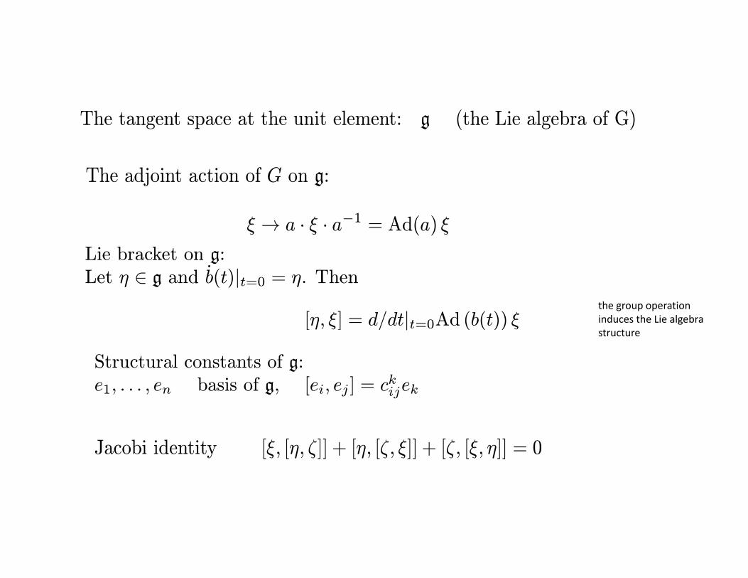
The tangent space at the unit element: g (the Lie algebra of G)

The adjoint action of G on g:

ξ → a · ξ · a−1 = Ad(a) ξLie bracket on g:Lie bracket on g:Let η ∈ g and b(t)|t=0 = η. Then

[η, ξ] = d/dt|t=0Ad (b(t)) ξthe group operation induces the Lie algebra [η, ξ] / |t=0 ( ( )) ξ

Structural constants of g:e1, . . . , en basis of g, [ei, ej ] = ckijek

structure

Jacobi identity [ξ, [η, ζ]] + [η, [ζ, ξ]] + [ζ, [ξ, η]] = 0

Coordinates on TG and T*G:Coordinates on TG and T G:

move the basis e1, …, en by the left multiplication to each point of the group

get a frame of left invariant vector fields, still denoted e1,…, en

Identify TG with G× g or with G×Rn by using the frame.

(a ξ) ∈ G× g→ a · ξ ∈ T G(a, ξ) ∈ G× g→ a ξ ∈ TaG

or

( a ; ξ1, . . . , ξn)→ a · (ξiei) ∈ TaG

Si il l T ∗G i id tifi d ith G ∗ ith G RnSimilarly, T ∗G is identified with G× g∗ or with G× Rn

(a,α) ∈ G× g∗ → (a∗)−1 · α ∈ T ∗a G

or

( a ; y1, . . . , yn) ∈ G×Rn → (a∗)−1(yje∗j ) ∈ T ∗aG

dual basis to e1,…,en

The coordinates y1, . . . , yn can also be thought of as functions on T ∗G.

Prolongation of the action of G on itself by the left multiplication to T ∗G:

b · ( a ; y1, . . . , yn) → ( ba , y1, . . . , yn)

Note that y y considered as functions on T*M are invariant underNote that y1, …, yn considered as functions on T*M are invariant under (the prolongation of) the left multiplication. This is more or less by definition.

C∞(G \ T*G) are exactly the functions of y1, …, yn.

Interpretation:T*G … we followa(t) and d/dt y(t) (momentum)

Y= G \ T*G reduced( \ ) y y1 yn

In fact, in this case Y = G \ T*G can be identified with Rn or g∗

Y= G \ T*G reducedphase space:we “forget” a(t)and follow only d/dt y(t)

The functions y1, …, yn provide coordinates on Y (which are global)

equations for y:C∞(Y) inherits a Poisson bracket from T*M. What is the bracket?

h l l Thi d li l k h i i

q yd/dt y(t) = H,y

hamiltonianH H( )enough to calculate y i, y j

Calculation: yI , yj = ckij y k

This needs a little work, the main pointis to use the formulade*j (ek , el)= ‐ e*j([e k, el])for the invariant forms/fields‐see next

H=H(y)

Calculation: yI , yj c ij y k,

where ckij are the structure constants of the Lie algebra g

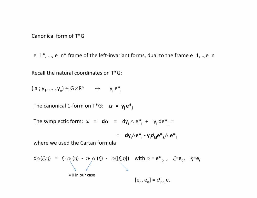
Canonical form of T*GCanonical form of T G

e_1*, …, e_n* frame of the left‐invariant forms, dual to the frame e_1,…,e_n

Recall the natural coordinates on T*G:

( ) G Rn *( a ; y1, … , yn) ∈ G×Rn ↔ yj e*j

The canonical 1‐form on T*G: α = yj e*j

The symplectic form: ω = dα = dyj Æ e*j + yj de*j =

= dyjÆe*j ‐ yjcjkle*kÆ e*l dyjÆe j yjc kle kÆ e l

where we used the Cartan formula

dα(ξ,η) = ξ· α (η) ‐ η· α (ξ) ‐ α([ξ,η]) with α = e*p , ξ=eq, η=erp q

= 0 in our case[ep, eq] = crpq er

In the local frame in T*G given by y1,…,yn, e1,…,en the form omega is given by the matrix

µ0 I−I −C(y)

¶with notation yk ckij ∼ C(y)

µ−I −C(y)

¶

The inverse ωrs of this (anti‐symmetric) matrix is given by ( y ) g y

µ−C(y) −I

I 0

¶µI 0

¶

The Poisson bracket is (in our conventions) f,g = ωrs fs grThe Poisson bracket is (in our conventions) f,g ω fs gr

In particular, yi , yj = ckij y k,

Remark:Note that the group G was any Lie group. We have shown:

If G is a Lie group and g is its Lie algebra ith structural constants ckIf G is a Lie group and g is its Lie algebra with structural constants ckij ,then on the dual g∗ of g the formula

yi, yj = ckijykyi, yj cijyk

defines a Poisson bracket on g∗.

This was already known to S. Lie, but he did explore the implications.

In the 1960s this structure was used by A. A. Kirillov to obtain importantresults in representations of nilpotent groups, and to develop his“method of orbits”.

b∈ G ⇒ the left shifts a ba extend to a symplectic diffeom of T*G:b∈ G ⇒ the left shifts a ba extend to a symplectic diffeom. of T G:

represent the form yi e*i at a

in the coordinates ( a , y1,…,yn): b·(a, y1, …, yn) = (ba, y1, … , yn)

h i fi i i l i f h d f ithe infinitesimal version of these deformations:

ξ ∈ g generates an infinitesimal symplectic deformation of T ∗G

y does not change, since the coordinate functionsyi are invariant under the left shifts

ba=(1+² ξ) a

( a , y ) ( a+² ξ·a , y )

Recall: Infinitesimal sympl. defs. functions (perhaps modulo corrections)

Wh t i th ti f ti f f ( ) ( + ξ ) ?What is the generating function f for ( a , y ) ( a+² ξ·a , y ) ?

In the coordinates of lecture 1 it would be f = pi ξi

We need to express this in the presently used coordinate frame y1,…, yn, e1, …, en

coordinates of the infinitesimal deformation in this frame:first coordinate

( 0 , … , 0 , [Ad (a‐1) ξ ]1 , … , [Ad (a‐1) ξ ]n )

need to use this form because our coordinate frame is left invariant (not right‐invariant).

no shift in y

arises from ξ · a = a a ‐1 · ξ · a = a · Ad (a‐1)ξ

(not right invariant).

Recall Noether’s Theorem: recall f = pi ξi in coordinatesof lecture 1

The generating function of the infinitesimal symplectic transformation above will be

f (a,y) = < y , Ad(a‐1) ξ > = < Ad(a‐1)* y , ξ >

Moreover f(a y) will be conserved for any Hamiltonian depending only on yMoreover, f(a,y) will be conserved for any Hamiltonian depending only on y

Exercise: check “by hand” that f , yi = 0 for each i

f Example: rigid body rotationDefinition:

M(a,y) = Ad(a‐1)* y ∈ g∗Example: rigid body rotationy momentum in the coordinate

frame moving with the bodyAd(a‐1)y momentum in thecoordinate frame fixed in space

is called the moment map.

For any Hamiltonian depending only on y the evolution preserves M or dM/dt 0For any Hamiltonian depending only on y the evolution preserves M, or dM/dt = 0.

This is because the ξ above can be taken as any element of g

“S l ti l ” f th P i if ld g∗ ( t d G)

determined by Ci(y)=ci, Ci the Casimir functions, Ci, yj=0 for each j=1,…,n

“Symplectic leaves” of the Poisson manifold g

A subspace through y generated by all possible

(a connected G)

y

A subspace through y generated by all possible vectors dy/dt=H,y, as H runs through all H=H(y)is contained in the tangent space to the orbit Oy = Ad*(a)y, a∈ G (because of the conservation of M for any such H, for example).

Vice versa, any vector in Ty Oy can be obtained in this way.orbit Oy in this way.

Hence: Symplectic leaves orbits

(See A A Kirillov’s book for more and implications to representations )(See A.A.Kirillov s book for more and implications to representations.)

Hence the evolution on g∗ given by H(y) and , really describes a family

of hamiltonian systems (parametrized by the orbits)

Example: non‐degenerate stationary points are (locally) parametrized by the orbits:

Non‐degenerate critical point of H on one orbits

manifold of stationarypoints (transversalto the orbit foliation)

point of H on one orbitsimplies critical points in neighboring orbits

orbits

Example: the simplest non‐commutative group G (Commutative G leads to yi, yj=0)

G = A =

µa b0 1

¶; a > 0, b ∈ R

the group of orientation‐preservingaffine transformation of R(maps of the form x ax+b ) with a>0

µ0 1

¶; > , ∈ ( p )

g = X =

µx y0 0

¶; x, y ∈ R

y

adjoint orbits

µ0 0

¶g∗ = P =

µp q0 0

¶; p, q ∈ R

x

< P, X >= px+ qyq

co‐adjoint orbits

Ad(A) ∼µ

1 0−b a

¶Ad(A)∗ ∼

µ1 −b0 a

¶p

µ ¶ µ ¶

bG e2=a/ be2* = db/a

Left invariant geodesics

e1=a/ae1*=da/a

given by Hamiltonian

H=H(p,q)=(p2+q2)/2 note the change of notation –both p and q are components of the momentum

1

e1 da/a

p,q = q

dp/dt = H,p = q2

of the momentum

ap/ ,p q

dq/dt = H,q = ‐ pq

Momentum conservation: geodesicsMomentum conservation:

da/dt = pa, db/dt = qa

geodesics

Example of solutions: a(t) = a0 tanh(t)b(t) = a0/cosh(t)

Poincare model of the hyperbolic plane G ∼

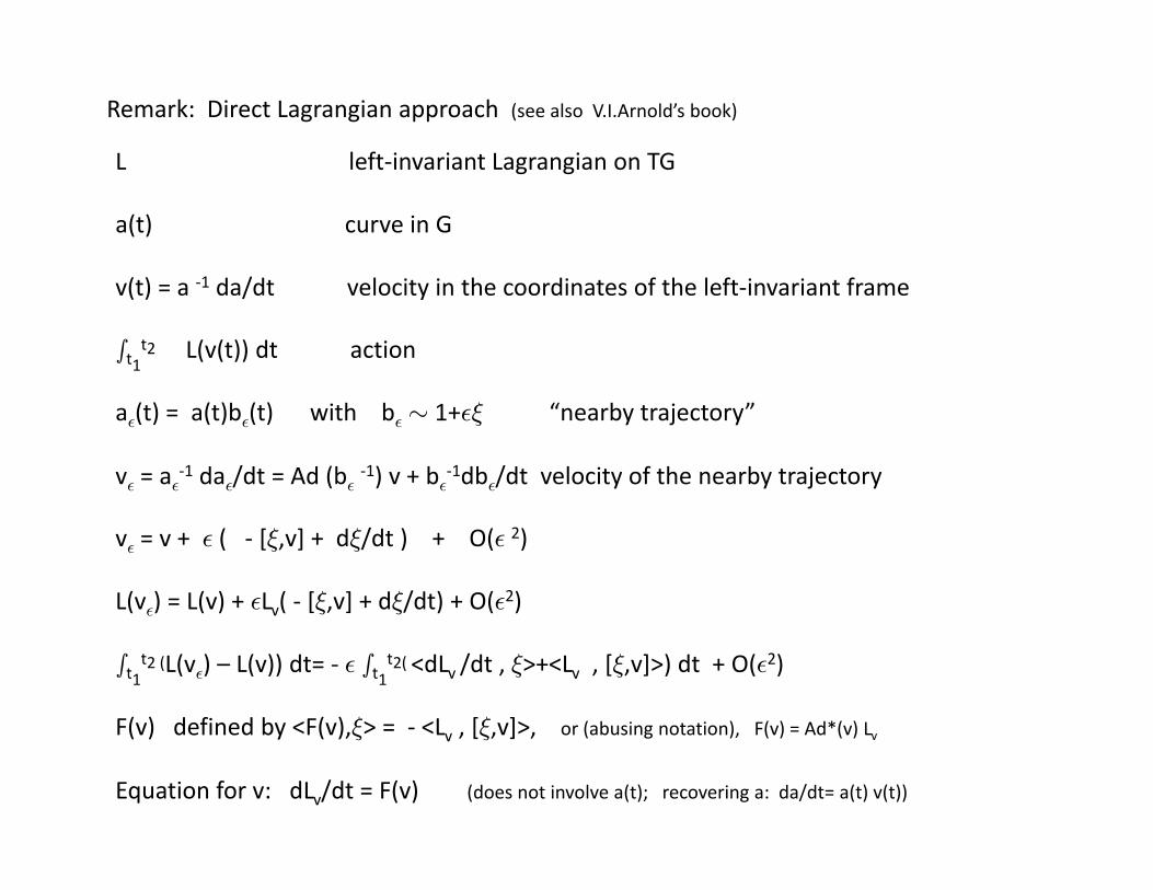
Remark: Direct Lagrangian approach (see also V.I.Arnold’s book)

L left‐invariant Lagrangian on TGL left invariant Lagrangian on TG

a(t) curve in G

1 /v(t) = a ‐1 da/dt velocity in the coordinates of the left‐invariant frame

∫t1t2 L(v(t)) dt action

a²(t) = a(t)b²(t) with b²∼ 1+²ξ “nearby trajectory”

v² = a²‐1 da²/dt = Ad (b²

‐1) v + b²‐1db²/dt velocity of the nearby trajectory

v² = v + ² ( ‐ [ξ,v] + dξ/dt ) + O(² 2)

L(v²) = L(v) + ²Lv( ‐ [ξ,v] + dξ/dt) + O(²2)² v ξ ξ

∫t1t2 (L(v²) – L(v)) dt= ‐ ² ∫t1

t2( <dLv /dt , ξ>+<Lv , [ξ,v]>) dt + O(²2)

F(v) defined by <F(v) ξ> = <L [ξ v]> or (abusing notation) F(v) Ad*(v) LF(v) defined by <F(v),ξ> = ‐ <Lv , [ξ,v]>, or (abusing notation), F(v) = Ad*(v) Lv

Equation for v: dLv/dt = F(v) (does not involve a(t); recovering a: da/dt= a(t) v(t))

Other calculable geodesics for left‐invariant metrics:

Sl(2,R) ∼ motion of a rigid body in the hyperbolic plane

H3 tree‐dimensional Heisenberg group, Caratheodory metrics

S3 or SO(3) ∼ three‐dimensional rigid body (Euler’s equations for rotating bodies)

and more ….

We expect: 3d group with a left invariant hamiltonianWe expect: 3d group with a left‐invariant hamiltonian⇒ co‐adjoint orbits have dimension at most 2 ⇒ equations for geodesics solvable by quadratures

On the other hand: 6d groups (such as Sl(2,C) or SO(4)) – will often have4d orbits – potential for “chaos” in the reduced equations

Special Hamiltonians can still give integrability:Kovalevskaya’s top, n‐dim rigid body in Euclidean space (Manakov)

Ideal Incompressible Fluids

n unit normal

p

u

C fi ti G Diff () l iConfiguration space: G=Diff0() volume‐preservingdiffeomorphisms of (group under map composition)

Motion the fluid: curves in G, t φt

φt(x)

t φt (x) trajectory of a “particle”

x

Symmetries: φt is a solution, ψ ∈ G ⇒ φ t ψ is a solution

“particle re‐labeling”

n Hamilton’s principle: the actual fluid motions “solutions”

uare extremals of Z t2 Z

| φt(x)|2 dx dt

φt(x)

Zt1

ZΩ

among curves φt in G with φt1 and φt2 fixed

xThis leads to Euler’s equations forThis leads to Euler s equations for

u(x, t) = φ( φ−1(x, t) , t )we are now using right shifts,rather then the left shifts….

It’s not hard to get the equation by direct calculation – but we will follow the Hamiltonian approach, which also immediatelly gives the conservation laws coming from the invariance by G (“particle re‐labelings”)

Th Li l b f G Diff () d it d lThe Lie algebra of G=Diff0 () and its dual

U = T G the Lie algebra of G ∼ div‐free vector fields in tangentU = Tidentity G ……… the Lie algebra of G ∼ div‐free vector fields in tangent to the boundary

U [ ] h l Li b k fu,v ∈ U …………[u,v] the usual Lie bracket of u,v (is exactly the bracket induced from the group)

φ

uφ#u

Adjoint action: Ad(φ) u = φ#u (φ#u)(x) = Dφ (φ‐1(x)) u(φ‐1(x))φ

φ ‐1(x) x

The dual U* linear functionals on U can be obtained most naturally by

u ∫ ai(x) ui(x) dx = <a,u>

where a is viewed as a 1‐form.

The co‐adjoint action (of G=Diff () on U*)The co‐adjoint action (of G=Diff0() on U )

<a, φ#u> = <φ*a , u> φ*a …… the usual pull‐back

[ φ*a (φ(x)) ] i = aj(x) φj,i(x)

Ad*(φ) a = φ*a

So it seems natural to identify U* with one‐forms, but the problem isthat the correspondence is not one‐to‐one:p

a = df ⇒ <a,u> = 0 for each u∈ U: ∫∇f u = ∫ ‐ f (div u) = 0

To get a one‐to‐one correspondence

replace 1‐forms by (1‐forms)/(exact differentials df)replace 1 forms by (1 forms)/(exact differentials df)

1‐forms / differentials df 2‐forms vector fieldsd via the volume element

ai dxi ai j dxjÆdxi ωi / x i , with ωi=²ijka k ji i,j / , k,j

Or, in the “vector calculus” notation:

( ) la ∼ (a1, a2, a3) ω = curl a

Action of Diff ()Action of Diff0 ()

in the “a‐coordinates” In the “ω‐coordinates”

Ad*(φ) a = φ*a Ad*(φ)ω = φ#ω

Duality in between U and U* in the ω‐coordinates on U*Duality in between U and U in the ω coordinates on U

a ∼ ai dxi da ∼ curl a ∼ ω ∼ ωi /x i

u ∈ U, u=curl Ψ , div Ψ = 0 in , ΨÆn = 0 on when is topologically trivial)

vector potential of u, analogue of the 2d stream function

f i li it l thi k f R3

∫ a u dx = ∫ ω Ψ dx (Check that the boundary term vanishes due to the boundary conditions)

for simplicity you can also think of = R3

In these “coordinates” the basic variable is ω = ω(x,t) (“vorticity”)

The vector fields u∈U are identified with their vector potentials Ψ

The Hamiltonian = kinetic energy : ω∈ U*, curl u = ω, div u = 0, un|=0, ‐∆ Ψ = ω, div Ψ = 0, ΨÆn| = 0

H = H(ω) = ∫ ½ |u|2 dx = ∫ ½ωΨ dx

Poisson bracket

Lie bracket in U in terms of the vector potentials Ψ

l Ψ l Φ U [ ] l Θu = curl Ψ, v = curl Φ ∈ U, w=[u,v], w=curl Θ

w = [u,v] = u∇v – v∇u = ‐ curl (uÆv) (we used div u = div v = 0)

Θ = ‐ curl Ψ Æcurl Φ

Ψ and Φ can be considered as linear function on U*Ψ and Φ can be considered as linear function on U*

lΨ : ω ∫ ωΨ and lΦ : ω ∫ ωΦ“variational derivative”,expressing F’ and G’

Poisson bracket: lΨ , lΦ = lΘ = l‐ curlΨ Æcurl Φ

expressing F and G using the duality with U(need some smothness)

general functionals: F , G (ω) = ∫ ω ( ‐ curl (δF/δω) Æ curl(δG/δω) ) dx

Example: H(ω) = ∫ ½ ω Ψ ( the Euler Lagrangian introduced earlier)Example: H(ω) = ∫ ½ ω Ψ ( the Euler Lagrangian introduced earlier)

δH/δω = Ψ (with ‐∆Ψ = ω + boundary cond.)

d/dt lΦ (ω) = ∫ ωtΦ = H , lΦ (ω) = ∫ ω( ‐ curl Ψ Æ curl Φ) = ∫ curl(ωÆu) Φ

ω = curl u, div u = 0 + boundary cond., u = curl Ψ

Φ is arbitrary div‐free with ΦÆn = 0 at the boundary

evolution of the “coordinate” given by ΦAnalogous to thefinite‐dimensionalequationdyi/dt=H,yi

ωt + curl (uÆω) = 0 or

ωt + [ u , ω ] = 0vorticity formulation of Euler’s equations

t

Noether’s theorem (conservation of the moment function)

Ad*(φt)‐1 ω(t) = ω(0) or ω(t) = φ# ω(0) Helmholtz’s law “vorticity moves with the flow”

Consequences of Helmholtz’s law

velocity ucurve γ

Vortex filament at initial time

ω

y

∫γ ui dxiis conserved(γmoving with the flow)

section S

∫S ωn is conserved(S moving with the flow)

folding necessarynot to increase energy

volume of the filamentvolume of the filamentmust be preserved

eventually it will presumablybecome very

velocity near the filament increases

become very complicated

ωvorticity is “stretched”

must become very thinat many places (preservationof volume) – high velocities,a lot of folding necessary so that energy is not increased

A benefit of the co‐adjoint orbit approach:j pp

some “reduced” systems (such as point vortices, vortex fillaments,…)come with natural hamiltonian structure.

1) 2d ….. sets of a given number of points can be moved around byDiff0() ‐ finite dimensional orbits – finite dimensional Hamiltoniansystem ‐ “point vortices” (Hamiltonian can be taken fromthe original Euler’s eq. if we remove the infinite “self‐energy”of each vortex.

2) 3d ….. curves can be moved around by Diff0()get a natural symplectic structure on the “manifold of curves”for certain “weak filaments” energy ∼ lengthcurves with the sympl. structure, Hamiltonian = length,‐ flow of curves by binormal curvature

Geometric picture of the steady‐states for 2d Euler:

manifold of stationarypoints (transversalto the orbit foliation)

Non‐degenerate critical point of H on one orbitsimplies critical points in neighboring orbits

)

orbits

Can be established rigorously in 2d under some (reasonable) assumptions(A. Choffrut, V.S.)

References:

V.I.Arnold: Mathematical Methods of Classical Mechanics

V.I.Arnold, B. A. Khesin: Topological Fluid Mechanics

A.A.Kirillov: Lectures on the orbit method

J.Marsden, A.Weinstein: Coadjoint orbits and Clebsch variables for incompressiblefluids, Physica D 7 (1983), no. 1‐3, 305 ‐ 323