Embed Size (px)
Citation preview

The Geometry ofClassical and Quantum Fields
Markus J. Pflaum
April 11, 2018

Authors
The following people have contributed to this work, in alphabetical order:
Jonathan BelcherMarkus J. Pflaum (main author)
ii

Copyright
Copyright c© 2017 Markus J. Pflaum. Permission is granted to copy and distribute thisdocument under the terms of the Creative Commons License Attribution-NonCommercial-NoDerivatives 4.0 International (CC BY-NC-ND 4.0).
iii
Contents
Preliminaries iTitlepage . . . . . . . . . . . . . . . . . . . . . . . . . . . . . . . . . . . . . . . . iAuthors . . . . . . . . . . . . . . . . . . . . . . . . . . . . . . . . . . . . . . . . . iiCopyright . . . . . . . . . . . . . . . . . . . . . . . . . . . . . . . . . . . . . . . . iiiContents . . . . . . . . . . . . . . . . . . . . . . . . . . . . . . . . . . . . . . . . . vAttribution . . . . . . . . . . . . . . . . . . . . . . . . . . . . . . . . . . . . . . . vi
Introduction 1
I. Classical Field Theory 2
1. Variational calculus 31.1. Euler–Lagrange equations . . . . . . . . . . . . . . . . . . . . . . . . . . . . 3
Regular domains . . . . . . . . . . . . . . . . . . . . . . . . . . . . . . . . . 3The local case . . . . . . . . . . . . . . . . . . . . . . . . . . . . . . . . . . . 3
II. Quantum Mechanics 5
2. The postulates of quantum mechanics 62.1. The geometry of projective Hilbert spaces . . . . . . . . . . . . . . . . . . . 62.2. Quantum mechanical symmetries . . . . . . . . . . . . . . . . . . . . . . . . 13
Automorphisms of the projective Hilbert space and Wigner’s theorem . . . 13Lifting of projective representations and Bargmann’s theorem . . . . . . . . 15
3. Deformation quantization 183.1. Fedosov’s construction . . . . . . . . . . . . . . . . . . . . . . . . . . . . . . 18
The various Weyl algebras of a Poisson vector space . . . . . . . . . . . . . 18The bundle of formal Weyl algebras . . . . . . . . . . . . . . . . . . . . . . 20Connections on the formal Weyl algebra . . . . . . . . . . . . . . . . . . . . 25
4. Molecular quantum mechanics 294.1. The von Neumann–Wigner no-crossing rule . . . . . . . . . . . . . . . . . . 29
III. Quantum Field Theory 31
5. Axiomatic quantum field theory a la Wightman and Garding 325.1. Wightman axioms . . . . . . . . . . . . . . . . . . . . . . . . . . . . . . . . 32
iv

5.2. Fock space . . . . . . . . . . . . . . . . . . . . . . . . . . . . . . . . . . . . . 34
IV. Mathematical Toolbox 36
6. Topological Vector Spaces 376.1. Seminorms, locally convex topologies, and convergence . . . . . . . . . . . . 376.2. Function spaces and their topologies . . . . . . . . . . . . . . . . . . . . . . 396.3. Summability . . . . . . . . . . . . . . . . . . . . . . . . . . . . . . . . . . . 40
7. Distributions and Fourier transform 417.1. Schwartz test functions . . . . . . . . . . . . . . . . . . . . . . . . . . . . . . 41
8. Hilbert Spaces 428.1. Inner product spaces . . . . . . . . . . . . . . . . . . . . . . . . . . . . . . . 428.2. Orthogonal decomposition and the Riesz representation theorem . . . . . . 488.3. The monoidal structure of the category of Hilbert spaces . . . . . . . . . . . 50
9. Manifolds 539.1. Pro-manifolds . . . . . . . . . . . . . . . . . . . . . . . . . . . . . . . . . . . 539.2. Hilbert manifolds . . . . . . . . . . . . . . . . . . . . . . . . . . . . . . . . . 53
10.Lie groups 5410.1. Symmetry groups of bilinear and sesquilinear forms . . . . . . . . . . . . . . 5410.2. The Lie group SOp3q and its universal cover SUp2q . . . . . . . . . . . . . . 5910.3. The Lorentz group SOp1, 3q and its universal cover SLp2,Cq . . . . . . . . . 65
11.Fiber bundles 6811.1. Fiber bundles . . . . . . . . . . . . . . . . . . . . . . . . . . . . . . . . . . . 68
Fibered manifolds and fibered charts . . . . . . . . . . . . . . . . . . . . . . 68
12.Jets 7012.1. A combinatorial interlude . . . . . . . . . . . . . . . . . . . . . . . . . . . . 70
Multiindices . . . . . . . . . . . . . . . . . . . . . . . . . . . . . . . . . . . . 70Multipowers and multiderivatives . . . . . . . . . . . . . . . . . . . . . . . . 73The formula of Faa-di-Bruno . . . . . . . . . . . . . . . . . . . . . . . . . . 74
12.2. Jet bundles . . . . . . . . . . . . . . . . . . . . . . . . . . . . . . . . . . . . 75
Licensing 78
CC BY-NC-ND 4.0 78
Bibliography 87
v

Attribution
The main author of this work is Markus J. Pflaum.
Jonathan Belcher took notes of several lectures by M.J. Pflaum in Fall 2017. The followingmaterial by J. Belcher has been incorporated in this work:
• Remark 2.1.8,
• in Section 2.2, notes on the statement of Theorem 2.2.5 (Wigner’s theorem), andTheorem 2.2.8 (Bargmann’s theorem),
• Proposition 10.3.3.
vi

Introduction
Classical and quantum mechanical systems are mathematically described in a different way.For finitely many degrees of freedom, differential geometry, notably symplectic and Pois-son geometry, provides the language in which classical mechanical systems are described,whereas functional analysis and in particular the theory of Hilbert spaces is the appropriatelanguage in which quantum mechanics is formulated. The mathematics is well understoodin both situations, and one even has a powerful tool for the passage from the classical to thequantum mechanical description of a corresponding system, namely quantization theory.
In their book Gustafson & Sigal (2011) on Mathematical Concepts of Quantum Mechanics,Gustafson and Sigal depicted the situation by the following diagram, where dÑ8 denotesthe passage from finitely to infinitely many degrees of freedom.
CM QM
CFT QFT
quantization
qÑ8 qÑ8
quantization
The key ingrediants for the description of a physical system are the mathematical objectswhich encode its state space, the observable space, and its dynamics. These objects shoulddepend in some functorial on the system and usually come from quite distinct categories,depending on whether the system is classical or quantum, has finitely or infintely manydegrees of freedom.
1
Part I.
Classical Field Theory
2

1. Variational calculus
1.1. Euler–Lagrange equations
Regular domains
Let M be a manifold of dimension d ą 0. By a regular domain in M we understand anon-empty open connected subset Ω Ă M such that the closure Ω possesses a smoothtriangulation κ : K Ñ Ω with the property that κ´1pBΩq is a simplicial subcomplex of Kof dimension ă d where BΩ denotes the (topological) boundary of Ω. Recall that κ being atriangulation means that K Ă Rn is a simplicial complex and that κ is a homeomorphismsuch that for every simplex σ P K the restriction κ|σ : σ Ñ κpσq is a diffeomorphism. Thatκ|σ is a diffeoemorphism just says that for every smooth f defined on an open neighborhoodof κpσq the pullback κ|˚σf can be extended to a smooth function on Rn and that for everysmooth g defined on an open neighborhood of the simplex σ Ă Rn the pullback
`
κ|´1σ
˘˚g
has a smooth extension to M .
In most applications and in particular in those which we will consider in this section, Ω willbe the interior of a submanifold-with-corners of M (see ?? for details on manifolds-with-corners and submanifolds in this category). In the proofs in this section involving regulardomains we will therefore consider mostly this particular case and only briefly indicate howthe argument in the more general situation goes. For ease of presentation we will call aregular domain Ω Ă M such that Ω Ă M is a submanfold-with-corners a strongly regulardomain.
The local case
Put M “ Rd and assume that Ω Ă M “ Rd is a regular domain. Denote the canonicalcoordinates of Ω by px1, . . . , xdq : Ω Ñ Rd. Further assume that π : E “M ˆ F ÑM is atrivial vector bundle with fiber F being a connected open subset of some euclidean space Rn.The canonical fiber coordinates will be denoted by pu1, . . . , unq : F Ñ Rn. The canonicalcharts of the base and fiber give rise to a fibered chart px, uq : E “ F ˆ Ω Ñ Ω ˆ Rn.Observe that Ω is oriented by the restriction of the canonical volume form dx1^ . . .^ dxnto Ω. Denote that restriction by ω. Note that the canonical charts xl of the base, thecanonical fiber charts uk and the canonical volume form all have unqiue extensions to theclosure Ω XM . We will denote those extensions by the same symbols as the unextendedfunctions.
Next we assume to be given a lagrangian function L P C8loc
`
J8π˘
. Since L is a localfunction on the jet bundle, it can be regarded as an element of C8
`
Jkπ˘
for some natural
3

1. Variational calculus 1.1. Euler–Lagrange equations
k. Let o “ opLq be the smallest of such numbers and call it the order of the langragianfunction. The canonical volume form ω together with the lagrangian L give rise to thelagrangian density L “ Lω on the jet bundle J8π. Before we can write down the actionfunctional induced by the lagrangian density L we need to fix some boundary conditions.For now, we will restrict to so-called Dirichlet boundary conditions. These are encoded bythe restriction to BΩ of compactly supported smooth sections s : Rn Ñ E. More preciseley,the space of Dirichlet boundary conditions (with compact support) over the domain Ω isdefined by
BC8D,cptpΩ;Eq “ Γ8cptpBΩ;Eq “
b P ΓpBΩ;Eqˇ
ˇ Ds P Γ8pRn;Eq : b “ s|BΩ(
.
Given an element b P BC8D,cptpΩ;Eq we single out the space X of allowable sections of E:
X “
s P Γ8cptpRn;Eqˇ
ˇ s|BΩ “ b(
.
In other words, X consists of all compactly supported smooth sections s of E which fulfillthe Dirichlet boundary condition s|BΩ “ b. Now we can write down the action functional:
(1.1.0.1) S : X Ñ R, s ÞÑż
Ω
`
j8s˘˚L “
ż
Ω
`
L ˝ j8s˘
ω .
4

Part II.
Quantum Mechanics
5
2. The postulates of quantum mechanics
2.1. The geometry of projective Hilbert spaces
2.1.1 Let H be a Hilbert space over the field K “ R or “ C. The associated projectivespace PpHq then is defined as the space of all rays in H that is as the space
PpHq “
l P PpHqˇ
ˇ l is a 1-dimensional K-subspace of H(
.
We will also call PpHq a projective Hilbert space. It carries a natural topology which wenow describe. Consider Hzt0u with its subspace topology. Then one has a natural map
π : Hzt0u Ñ PpHq, v ÞÑ Kv
which obviously is surjective. One endows PpHq with the final topology with respect to π.Next let us introduce an equivalence relation „ on Hzt0u by defining v „ w if there existsa λ P Kˆ “ Kzt0u such that v “ λw. Obviously „ is reflexive, since 1 P Kˆ, symmetric,since with λ P Kˆ the inverse λ´1 is in Kˆ as well, and transitive, since the product oftwo elements of Kˆ is in Kˆ. Hence „ is an equivalence relation indeed. Denote by pvthe equivalence class of an element v P Hzt0u. Let pH be the quotient space Hzt0u„ andpπ : Hzt0u Ñ pH the quotient map.
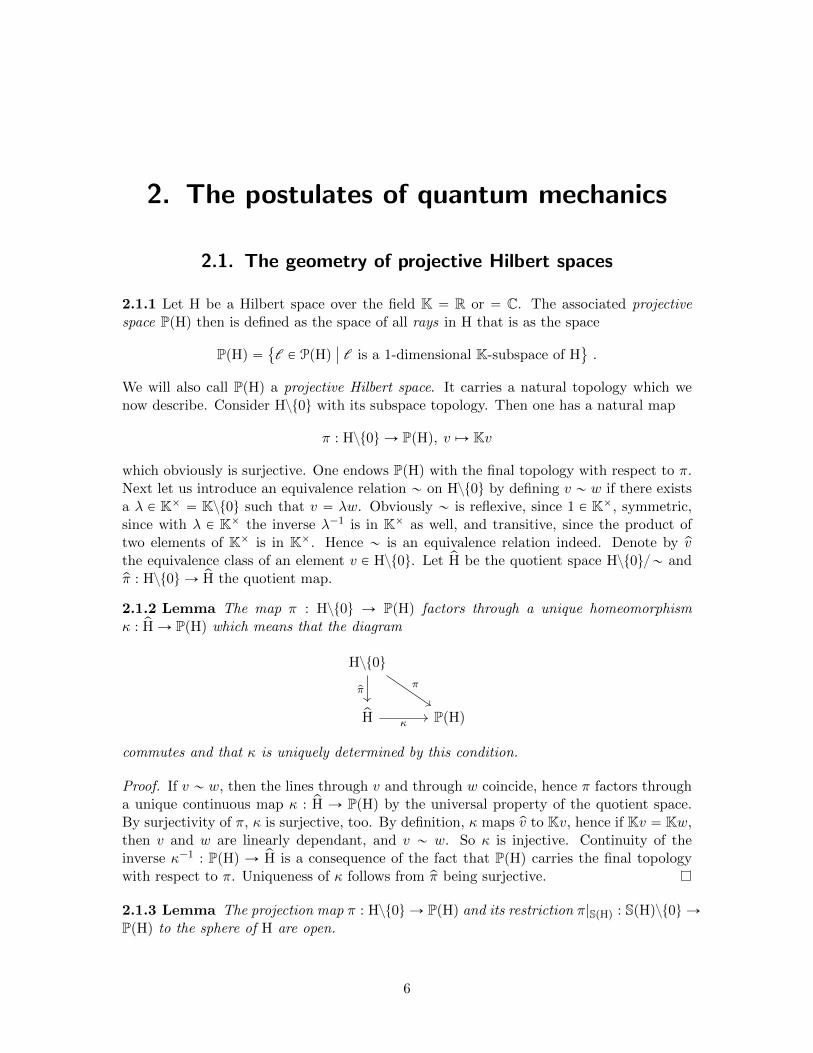
2.1.2 Lemma The map π : Hzt0u Ñ PpHq factors through a unique homeomorphismκ : pH Ñ PpHq which means that the diagram
Hzt0u
pH PpHq
πpπ
κ
commutes and that κ is uniquely determined by this condition.
Proof. If v „ w, then the lines through v and through w coincide, hence π factors througha unique continuous map κ : pH Ñ PpHq by the universal property of the quotient space.By surjectivity of π, κ is surjective, too. By definition, κ maps pv to Kv, hence if Kv “ Kw,then v and w are linearly dependant, and v „ w. So κ is injective. Continuity of theinverse κ´1 : PpHq Ñ pH is a consequence of the fact that PpHq carries the final topologywith respect to π. Uniqueness of κ follows from pπ being surjective.
2.1.3 Lemma The projection map π : Hzt0u Ñ PpHq and its restriction π|SpHq : SpHqzt0u ÑPpHq to the sphere of H are open.
6

2. The postulates of quantum mechanics 2.1. The geometry of projective Hilbert spaces
Proof. By the preceding lemma it suffices to show that pπ : Hzt0u Ñ pH is open. LetU Ă Hzt0u be open. Then
pπ´1`
pπpUq˘
“ď
λPKˆλ ¨ U ,
which is again open and the first part of the claim is proved. The second part follows inthe same way, since
pπ|´1SpHq
`
pπ|SpHqpUq˘
“ď
λPSpKqλ ¨ U
is open for all U Ă SpHq open.
2.1.4 Remark Strictly speaking, the projective space PpHq depends on the ground fieldK. If H is a complex Hilbert space one therefore sometimes writes RPpHq or CPpHq todenote that the projective space of all real respectively all complex lines is meant. In thiswork we agree that for H complex PpHq always stands for the projective space of complexlines in H. If we want to consider the projective space of real lines in some complex Hilbertspace H instead, we write RPpHq.
2.1.5 The inner product on the underlying Hilbert space H induces the projective innerproduct or ray inner product
|x¨, ¨y| : PpHq ˆ PpHq Ñ r0, 1s, pKv,Kwq ÞÑ |xKv,Kwy| “| xv, wy |
v w, where v, w P Hzt0u,
on the associated projective space. Note that the projective inner product is well-defined,since |xv,wy|
v w is homogeneous of degree 0 both in v and w.
Now we can formulate the first postulate of quantum mechanics.
(QM1) The state space of a quantum mechanical system is accomplished by a projectivespace PpHq associated to a complex separable Hilbert space H. The elements v PHzt0u are called state vectors, the rays l P PpHq are the pure states.
If a quantum mechanical system is prepared so that it is in the state l P PpHq, theprobability that a measurement detects the system to be in the state k P PpHq isgiven by the transition probability |xk,ly|2.
Because of their appearance in the first postulate of quantum mechanics we want to studyprojective Hilbert spaces in some more depth. We will use topological, geometric andanalytic tools for that endeavor. A first result is the following.
2.1.6 Theorem Let PpHq be the projective space of a Hilbert space of dimension ě 2 overthe field K of real or complex numbers. Then the following holds true:
(i) The projective Hilbert space PpHq is a completely metrizable topological space.
(ii) A complete metric inducing the topology on PpHq is given by
d : PpHq ˆ PpHq Ñ Rě0, pk,lq ÞÑ inf
v ´ wˇ
ˇ v P k, w P l & v “ w “ 1(
.
7

2. The postulates of quantum mechanics 2.1. The geometry of projective Hilbert spaces
(iii) The metric d and the transition probabilities are related as follows, where k,l P PpHq:
d2pk,lq “ 2`
1´ |xk,ly|˘
,(2.1.6.1)
d2pk,lq ě 1´ |xk,ly|2 .(2.1.6.2)
(iv) The Fubini–Study distance
dFS : PpHq ˆ PpHq Ñ Rě0, pk,lq ÞÑ arccos |xk,ly| .
is a metric on PpHq which is equivalent to the metric d. The diameter of PpHq withrespect to the Fubini–Study distance equals π
2 .
(v) The mapping P : PH Ñ BpHq which associates to every ray k the orthogonal projec-tion onto it is a bi-Lipschitz embedding. More precisely, the operator norm distancerestricted to PH satisfies for all k,l P PH
(2.1.6.3)1
2d2pk,lq ď P pkq ´ P plq2 “ 1´ |xk,ly|2 ď d2pk,lq .
Proof. ad (ii)Let us first show that the map d is a metric indeed. By definition, d is non-negative and symmetric. Assume dpk,lq “ 0 for two rays k,l. For given unit vectorsv P k and w P l there then exists a sequence pσkqkPN Ă S1 such that
limkÑ8
v ´ σkw “ 0 .
By compactness of S1 we can assume that the sequence pσkqkPN converges after possiblypassing to a subsequence. Let σ P S1 be its limit. Then v ´ σw “ 0, hence k “ l. Nowlet k,l,j P PpHq and z P j a representing unit vector. Then
dpk,lq “ inf
v ´ wˇ
ˇ v P k, w P l & v “ w “ 1(
ď
ď inf
v ´ z ` z ´ wˇ
ˇ v P k, w P l & v “ w “ 1(
“
“ inf
v ´ zˇ
ˇ v P k & v “ 1(
` inf
z ´ wˇ
ˇ w P l & w “ 1(
“
“ dpk,jq ` dpj,lq ,
hence d satisfies the triangle inequality, and therefore is a metric.
Next we prove that the metric topology of d coincides with the quotient topology of π. Letv, w P SpHq. By definition of the metric d one then has
dpKv,Kwq ď v ´ w .
This implies that for all ε ą 0
π´
BSpHqpv, εq¯
Ă BPpHqpKv, εq ,
where BSpHqpv, εq denotes the ε-ball around v in the sphere with respect to the norm andBPpHqpKv, εq the ε-ball around Kv in the projective Hilbert space with respect to the metricd. Hence the quotient topology on PpHq is finer than the metric topology. If for given ε ą 0a δ ą 0 is chosen so that δ ă ε, then for every ray l with dpKv,lq ă δ there exists an
8

2. The postulates of quantum mechanics 2.1. The geometry of projective Hilbert spaces
element w P l X SpHq such that v ´ w ă ε which means that l “ πpwq P π`
Bpv, εq˘
.Hence
BPpHqpKv, δq Ă π´
BSpHqpv, εq¯
and the quotient topology on PpHq is coarser than the metric topology. So d induces thetopology on PpHq as claimed.
It remains to verify that d is a complete metric. To this end observe first that for everyv P SpHq and ray l there exists a representative w P l X SpHq such that xv, wy “ |xKv,ly|.We will call such a representative of l distinguished with respect to v. Now let plnqnPN bea Cauchy sequence of rays. Then there exists an increasing sequence of natural numbersn0 ă . . . ă nk ă nk`1 ă . . . such that
dpln,lmq ă1
2k`1for all n,m ě nk .
Choose a representative v0 P ln0 X SpHq and let v1 P SpHq be a representative of ln1
distinguished with respect to v0. Then
v1 ´ v0 “a
2p1´Re xv0, v1yq “a
2p1´ |xln0 ,ln1y|q “ dpln0 ,ln1q ă1
2.
Now assume we have constructed v0, . . . , vk P SpHq such that Kvl “ lnl for l “ 0, . . . , kand such that for l “ 0, . . . , k ´ 1
(2.1.6.4) vl`1 ´ vl ă1
2l`1.
Let vk`1 P SpHq be a representative of lnk`1distinguished with respect to vk. Then
vk`1 ´ vk “a
2p1´Re xvk`1, vkyq “b
2p1´ˇ
ˇ
@
lnk`1,lnk
D
ˇq “ dplnk`1,lnkq ă
1
2k`1.
We thus obtain a sequence pvkqkPN in H such that (2.1.6.4) is fulfilled for all l P N. Thesequence pvkqkPN is even a Cauchy sequence since for n ě m ě k
vn ´ vm ďn´1ÿ
k“m
vk`1 ´ vk ăn´1ÿ
k“m
1
2k`1ă
1
2k.
Let v P H be its limit. Then
limkÑ8
dpKv,lnkq ď limkÑ8
v ´ vk “ 0 .
Hence the sequence of rays plnqnPN converges to the ray Kv and PpHq is complete withrespect to the metric d. Claim (i) is now proved as well.
ad (iii)Let k,l be rays in H and v P k, w P l representing unit vectors. Let λ P S1 suchthat xv, wy “ λ |xk,ly| and σ P S1 arbitrary. Then compute
v ´ σw2 “ 2`
1´Re xv, σwy˘
“ 2`
1´ |xk,ly|Reσλ˘
ě 2`
1´ |xk,ly|˘
.
9

2. The postulates of quantum mechanics 2.1. The geometry of projective Hilbert spaces
For σ “ λ, equality holds, hence
d2pk,lq “ inf!
v ´ σw2ˇ
ˇ σ P S1)
“ 2`
1´ |xk,ly|˘
.
With k,l, v, w as before and δ “ dpk,lq, the claimed inequality now follows immediately:
d2pk,lq ě δ2
ˆ
1´1
4δ2
˙
“ 2`
1´ |xk,ly|˘
ˆ
1´1
2
`
1´ |xk,ly|˘
˙
“ 1´ |xk,ly|2 .
ad (iv)The map dFS is symmetric by symmetry of the projective inner product. Notethat under the assumption dim H ě 1 the image of |x¨, ¨y| is the whole interval r0, 1s, sincePpHq is connected, since |x¨, ¨y| is bounded by 1 by the Cauchy–Schwarz inequality, since|xl,ly| “ 1 for every ray l and finally since there exist orthogonal rays. The image ofdFS therefore coincides with r0, π2 s which already entails the claim about the diameter. Bystrict monotony of arccos, dFSpk,lq “ 0 if and only if |xk,ly| “ 1. By (2.1.6.1) this is thecase if and only if dpk,lq “ 0 which means if and only if k “ l. Let us now show that dFS
satisfies the triangle inequality. To this end let k,l,j be rays in H. If the Fubini–Studydistance between any two of these rays is zero, the triangle inequality obviously holds true,so we exclude that case. Choose representatives v P k, w P l, z P j such that all havenorm 1. After possibly multiplying v and z by elements of S1 XK one can achieve that
xv, wy “ |xk,ly| and xw, zy “ |xl,jy| .
Let θ “ arccos xv, wy and ϕ “ arccos xw, zy. Then θ “ dFSpk,lq and ϕ “ dFSpl,jq. Nowlet x be a unit vector in the plane through v and w which is orthogonal to w and y a unitvector in the plane through w and z which is orthogonal to w. After possibly multiplyingx and y by elements of S1 XK one can achieve that xv, xy , xz, yy P r0, 1s. Then
v “ xv, wy w ` xv, xy x and z “ xz, wy w ` xz, yy y .
By θ, ϕ P“
0, π2‰
and xv, xy , xz, yy ě 0 one concludes
v “ cos θ w ` sin θ x and z “ cosϕ w ` sinϕ y .
Hence, by the triangle inequality for the absolute value and the Cauchy–Schwarz inequality
|xv, zy| “ |cos θ cosϕ` sin θ sinϕ xx, yy| ě cos θ cosϕ´ sin θ sinϕ “ cospθ ` ϕq .
Since arccos is monotone decreasing, one obtains
dFSpk,jq “ arccos |xv, zy| ď θ ` ϕ “ dFSpk,lq ` dFSpl,jq .
So the Fubini–Study distance satisfies the triangle inequality and is a metric indeed.
Last we need to prove that the Fubini–Study distance is equivalent to d. To this endconsider the functions
f :”
0,?
2ı
Ñ R, s ÞÑ arccos
ˆ
1´s2
2
˙
and g :”
0,π
2
ı
Ñ, t ÞÑa
2p1´ cos tq .
10

2. The postulates of quantum mechanics 2.1. The geometry of projective Hilbert spaces
Then both functions are continuous and differentiable on the interior of their domains.Now observe that fp0q “ gp0q “ 0 and compute
f 1psq “s
c
1´´
1´ s2
2
¯2“
sb
s2 ´ s4
4
“2
?4´ s2
ď?
2 for s P´
0,?
2¯
and
g1ptq “
?2
2
sin t?
1´ cos t“
?2
2
?1` cos t ď 1 for t P
´
0,π
2
¯
.
By definition of dFS and (2.1.6.1) the mean-value theorem then entails
dpk,lq “ g`
dFSpk,lq˘
ď dFSpk,lq “ f pdpk,lqq ď?
2 dpk,lq for all k,l P PpHq .
Hence d and dFS are equivalent metrics.
ad (v)Recall that the operator norm distance of P pkq and P plq is given by
(2.1.6.5) P pkq ´ P plq “ sup ›
›
`
P pkq ´ P plq˘
z›
›
ˇ
ˇ z P SpHq(
.
Choose normalized representatives v P k and w P l. After possibly multiplying w by acomplex number of modulus 1 we can assume that xv, wy “ |xk,ly| ě 0. If xv, wy “ 1 orin other words if v and w are linearly dependent then k and l coincide and the claim istrivial, so we assume that v and w are linearly independent. First we want to show that
(2.1.6.6)›
›
`
P pkq ´ P plq˘
z›
› ď 1´ |xv, wy|2 for all z P SpHq .
To this end expand z “ z‖ ` zK, where z‖ lies in the plane spanned by v and w and zK isperpendicular to that plane. Then
`
P pkq ´ P plq˘
z “ xz, vy v ´ xz, wyw “A
z‖, vE
v ´A
z‖, wE
w “`
P pkq ´ P plq˘
z‖ .
Hence it suffices to verify (2.1.6.6) for z P SpHq X spantv, wu. Observe that there existunique elements ϕ P r0, π2 s and µ P S1 XK such that xz, vy “ µ cosϕ. One can then find anormalized vector wK P spantv, wu perpendicular to v such that
µz “ cosϕv ` sinϕwK .
Note that with this
w “ xv, wy v `@
w,wKD
wK and |@
w,wKD
|2 “ 1´ | xv, wy |2 .
Now compute
›
›
`
P pkq ´ P plq˘
z›
›
2“
›
›
`
P pkq ´ P plq˘
µz›
›
2“ xz, vy v ´ xz, wyw2 “
“ | xµz, vy |2 ´ 2 xv, wy Re pxµz, vy xµz,wyq ` | xµz,wy |2 “
“ cos2ϕ´ 2 cosϕ xv, wy`
cosϕ xv, wy ` sinϕRe@
w,wKD˘
` cos2ϕ | xv, wy |2 ` 2 cosϕ xv, wy sinϕRe@
w,wKD
` sin2ϕ |@
w,wKD
|2 “
“ 1´ | xv, wy |2 .
11

2. The postulates of quantum mechanics 2.1. The geometry of projective Hilbert spaces
This proves (2.1.6.6), but also implies by (2.1.6.5) that
P pkq ´ P plq2 “ 1´ | xv, wy |2 “ 1´ |xk,ly|2 .
The claim now follows by (iii) and the theorem is proved.
After having examined some topological properties of projective Hilbert spaces we comenow to their differential geometry.
2.1.7 Theorem The projective Hilbert space PpHq of a Hilbert space of dimension ě 2over K has the following differential geometric properties:
(i) PpHq carries a natural structure of an analytic manifold modelled on a Hilbert spaceisomorphic to each of the Hilbert spaces Vw “ pKwqK, where w P H is a unit vector.
(ii) Let SpHq Ă Hzt0u be the sphere in H. Then the map
π|SpHq : SpHq Ñ PpHq, v ÞÑ Kv
is a smooth fiber bundle with typical fiber S1.
(iii) Endow SpHq with the riemannian metric gSpHq inherited from the ambient Hilbertspace. Then there exists a unique riemannian metric gFS on PpHq such that π|SpHq :SpHq Ñ PpHq becomes a riemannian submersion. This metric is called the Fubini–Study metric. Its geodesic distance coincides with the Fubini–Study distance dFS.
(iv) In case H is a complex Hilbert space, the projective space PpHq carries in a naturalway the structure of a Kahler manifold. Its complex structure is the one inheritedfrom H, and its riemannian metric is the Fubini–Study metric.
Proof. ad (i)For a given unit vector w P SpHq consider the linear form w5 : H Ñ K,v ÞÑ xv, wy. Let Vw “ kerw5 “ pKwqK and Uw “ π
`
HzVw
˘
. Then, by Theorem 8.2.3,one has the orthogonal decomposition H “ Vw ‘ Kw which gives rise to the orthogonalprojection prVw : H Ñ Vw. Next observe that Uw Ă PpHq is open since π´1pUwq “ HzVw
is open and PpHq carries the quotient topology with respect to π. Now we can define achart hw : Uw Ñ Vw by
hwpKvq “ prVw
ˆ
v
xv, wy
˙
for v P HzVw .
The map hw is well-defined since xv, wy ‰ 0 for all v P HzVw and since vxv,wy “
λvxλv,wy for
all λ P Kˆ. Moreover, hw is continuous by continuity of the composition hw ˝ π|HzVw . IfhwpKvq “ hwpKv1q, then
prVw
ˆ
v
xv, wy´
v1
xv1, wy
˙
“ 0 and
B
v
xv, wy´
v1
xv1, wy, w
F
“ 0,
hence Kv “ Kv1, so hw is injective. The map Vw Ñ Uw, y ÞÑ πpy ` wq is obviouslycontinuous and inverse to hw since hw
`
πpy ` wq˘
“ y for all y P Vw and since hw isinjective. So we have proved that hw : Uw Ñ Vw is a homeomorphism.
12

2. The postulates of quantum mechanics 2.2. Quantum mechanical symmetries
Next observe that all the Hilbert spaces Vw, w P SpHq are pairwise isomorphic since eachof them has codimension 1 in H. After this observation we show that for all v, w P SpHq
(2.1.7.1) hwpUw X Uvq “ Vwz p´prKv w `Vw XVvq .
Assume that y P Vw. The relation v R p´prKv w `Vw XVvq then is equivalent to prKvpy`wq ‰ 0, which on the other hand is equivalent to the existence of some λ P Kˆ and x P Vv
such that y`w “ λpx`vq. Since h´1w pyq “ πpy`wq, the latter is equivalent to the existence
of an x P Vv such that h´1w pyq “ πpx ` vq. But that is equivalent to h´1
w pyq P Uw X Uv.This proves (2.1.7.1).
The transition map between the chart hw and the chart hv is now given by
hv ˝ h´1w : Vwz p´prKv w `Vw XVvq Ñ Vvz p´prKw v `Vw XVvq , y ÞÑ prVv
y ` w
xy ` w, vy.
But this map is analytic as a composition of analytic maps, hence any two charts areCω-compatible. Since PpHq is obviously covered by the open domains Uw, w P SpHq, theprojective Hilbert space PpHq becomes an analytic manifold as claimed and that it is locallymodelled on a Hilbert space isomorphic to each of the Vw, w P SpHq.
2.1.8 Remark Notice that the chart hw in the proof of (i) can be written as
hwpCvq “v
xv, wy´ w .
This is the same as for the charts of finite dimensional projective space KPn. Indeed, wecan choose w as a basis element, say ek, k “ 0, . . . , n and we have a line
rv0 : . . . : vk : . . . : vns P KPn
represented by the vector v “ pv0, . . . , vk, . . . , vnq, where vk ‰ 0. Then the standard chart isobtained as follows. First normalize the vector representing the line in the k-th coordinate,i.e. divide by xv, wy:
„
v0
vk: . . . : 1 : . . . :
vnvk
,
and then map this to Kn via dropping the 1 in the k-th coordinate:
„
v0
vk: . . . : 1 : . . . :
vnvk
ÞÑ
ˆ
v0
vk, . . . ,
vk´1
vk,vk`1
vk, . . . ,
vnvk
˙
.
2.2. Quantum mechanical symmetries
Automorphisms of the projective Hilbert space and Wigner’s theorem
2.2.1 Assume that a quantum mechanical system is described by the projective Hilbertspace PH and that two observers O and O1 observe the system. While observer O describesthe states the system is in by rays k,l,li, , ... P PH, observer O1 describes them by possibly
13

2. The postulates of quantum mechanics 2.2. Quantum mechanical symmetries
different rays k1,l1,l1i , ... P PH. In other words this means that from the point of physicsthe rays are not invariant under observer change. Rather does the observer change giverise to a map A : PH Ñ PH, l ÞÑ Al “ l1. This map has to be invertible becausethe observer change is reversible. Even though rays describing the states of the systemdo change under an observer change, the corresponding transition probabilities remaininvariant by the paradigm that the laws of (quantum) physics do not change from oneobserver to another. Mathematically this can be expressed by
|xAk, Aly|2 “ |xk,ly|2 for all k,l P PH .
This leads us to the following definition.
2.2.2 Definition Let PH1 and PH2 be two projective Hilbert spaces. A map A : PH1 Ñ
PH2 such that|xAk, Aly| “ |xk,ly| for all k,l P PH1
is called an isometry from PH1 to PH2. A bijective isometry A : PH Ñ PH on a projectiveHilbert space PH is called an isometric automorphism, a Wigner automorphism or just anautomorphism.
In quantum mechanics, an automorphism of a projective Hilbert space PH is called asymmetry of the quantum mechanical system described by PH.
2.2.3 Because the composition of isometric maps between projective Hilbert spaces is anisometric map and the identity map on a projective Hilbert space is isometric the projectiveHilbert spaces as objects and the isometric maps as morphisms form a category whichwe call the Wigner category denoted by Wig. The Wigner automorphisms are then theautomorphisms of that category indeed.
The automorphisms of a projective Hilbert space PH form a group denoted by AutpPHq.
2.2.4 From now on in this section let the symbol H stand for a complex Hilbert spaceof dimension ě 2. We want to examine what maps on H induce automorphisms of thecorresponding projective Hilbert space.
If S : H Ñ H is a unitary operator that is S P GLpHq and xSv, Swy “ xv, wy for allv, w P H, then S : PH Ñ PH, Cv ÞÑ CSv is well-defined and an automorphism of PH. Butnot every automorphism of PH is of the form S with S P UpHq. Namely let T : H Ñ Hbe an anti-unitary map that is T P GLpH,Rq, T pλvq “ λTv for all v P H, λ P C andxTv, Twy “ xv, wy “ xw, vy for all v, w P H. Then T : PH Ñ PH, Cv ÞÑ CTv is alsowell-defined, invertible and preserves transition probabilities. Therefore T P AutpPHq. Wewill later see that T is not equal to any of the automorphisms S with S P UpHq. Observealso that by the dimension assumption on H there exists an anti-unitary transformation,for example the real linear map T : H Ñ H which acts on some initially chosen Hilbertbasis pvjqjPJ by T pvjq “ vj and T pivjq “ ´ivj .
One easily checks that the products ST and TS of a unitary operator S : H Ñ H and ananti-unitary operator T : H Ñ H are anti-unitary. If T1, T2 : H Ñ H are both anti-unitary,
14

2. The postulates of quantum mechanics 2.2. Quantum mechanical symmetries
then the product T1T2 is unitary. Hence we obtain a new group AUpHq consisting of allunitary and anti-unitary operators on H. The map
π : AUpHq Ñ AutpPHq, S ÞÑ S
then is a group homomorphism. Its kernel coincides with Up1q – S1. To see this letπpSq “ idPH. Then for every ray l there exists a complex number µl such that Sv “ µCvvfor all v P l. By unitarity |µl| “ 1. Let v, w P H be two linearly independant vectors ofnorm 1. Since
µCpw´vqpw ´ vq “ Spw ´ vq “ µCww ´ µCvv ,
one has 0 “ pµCpw´vq ´ µCwqw ` pµCv ´ µCpw´vqqv which implies µCw “ µCpw´vq “ µCv bylinear independence of v and w. Hence all the µCv coincide and S “ µ idH for some complexnumber µ P Up1q – S1. A consequence of this observation is also that the homomorphismπ|UpHq : UpHq Ñ AutpPHq, S ÞÑ S is not surjective because for every anti-unitary T andunitary S the product TS´1 is anti-unitary, hence can not be an element of Up1q. We denotethe image of UpHq under π by UpPHq and call its elements the unitary automorphisms ofPH.
2.2.5 Theorem (Wigner’s theorem, Wigner (1944)) Let H be a complex Hilbert spaceof dimension ě 2. Then the sequence of group homomorphisms
1 ÝÑ Up1q ÝÑ AUpHqπÝÑ AutpPHq ÝÑ 1
is exact.
2.2.6 Remark Wigner’s theorem was first stated in Wigner (1944), but with an incom-plete proof. Only several years later complete and independent proofs of Wigner’s resultwere given by Uhlhorn (1962), Lomont & Mendelson (1963), and Bargmann (1964).
Proof. Wigner’s theorem is an immediate consequence of the precedinmg considerationsand the following more general result.
2.2.7 Theorem (Optimal version of Wigner’s theorem, Geher (2014)) Let H be acomplex Hilbert space of dimension ě 2. Then for every isometry A : PH Ñ PH there existsa linear or conjugate-linear isometry S : H Ñ H such that A “ S, where S is the isometryon PH which maps the ray Cv with v P Hzt0u to the ray CSv.
Proof. To prove the claim we will follow the elementary argument by Geher (2014).
Lifting of projective representations and Bargmann’s theorem
2.2.8 Theorem (Bargmann’s Theorem) Let H be a complex Hilbert space and G aconnected and simply connected Lie group with H2pg,Rq “ 0. Then every projective rep-resentation τ : GÑ UpPHq can be lifted to a unitary representation σ : GÑ UpHq that isπ ˝ σ “ τ , where π : UpHq Ñ UpPHq is the canonical projection.
2.2.9 Remark The lifting theorem was proved first in Bargmann (1954). The short proofwe present here goes back to Simms (1971). We closely follow his argument.
15

2. The postulates of quantum mechanics 2.2. Quantum mechanical symmetries
Proof of the theorem. Let E be the fibered product of π and τ with the canonical homo-morphisms rτ : E Ñ UpHq and πE : E Ñ G. For the resulting commutative diagram ofgroups with two exact rows
1 Up1q E G 1
1 Up1q UpHq UpPHq 1
id
πE
rτ τ
π
we want to construct a section s : G Ñ E of πE : E Ñ G which is a splitting meaningthat s is a group homomorphism and πE ˝ s “ idG. With the construction of such ans we are done because then the unitary representation rτ ˝ s is a lifting of the projectiverepresentation τ : GÑ UpPHq.
Observe that E is a Lie group by Kuranishi’s theorem, see (Montgomery & Zippin, 1955,§4.3), since E is central extension of a Lie group, hence locally compact, and there existlocal continuous sections σ : U Ñ E that is U Ă G is open and πE ˝ σ “ idU .
The short exact sequence of Lie groups
1 ÝÑ Up1q ÝÑ EπEÝÝÑ G ÝÑ 1
induces a short exact sequence of Lie algebras
(2.2.9.1) 0 ÝÑ R ÝÑ eTπEÝÝÝÑ g ÝÑ 0 ,
where e is the Lie algebra of E and g the one of G. Observe that TπE is surjective withkernel R being in the center of e. Choose a linear map λ : g Ñ e such that πE ˝ λ “ idg.Put Θpx, yq “ rλpxq, λpyqs ´ λprx, ysq for all x, y P g. Then
TπE ˝Θpx, yq “ rTπE ˝ λpxq, TπE ˝ λpyqs ´ TπE ˝ λprx, ysq “ rx, ys ´ rx, ys “ 0 .
Hence Θpx, yq is in the kernel of TπE which means that Θ is a map g ˆ g Ñ R. Bydefinition, Θ : g ˆ g Ñ R is skew symmetric. Let us show that it satisfies the Jacobiidentity. Compute, using the Jacobi identity for the Lie algebra bracket and the fact thatΘ has image in the center of e,
Θprx, ysq, zq`Θpry, zs, xq `Θprz, xs, yq “
“ rλprx, ysq, λpzqs ` rλpry, zsq, λpxqs ` rλprz, xsq, λpyqs´
´ λprrx, ys, zsq ´ λprry, zs, xsq ´ λprrz, xs, ysq “
“ rrλpxq, λpyqs, λpzqs ` rrλpyq, λpzqs, λpxqs ` rrλpzq, λpxqs, λpyqs´
´ rΘprx, ysq, λpzqs ´ rΘpry, zsq, λpxqs ´ rΘprz, xsq, λpyqs “ 0 .
Therefore, Θ is a Lie algebra 2-cocycle. By H2pg,Rq “ 0, there exists a linear θ : g Ñ Rsuch that Θpx, yq “ θprx, ysq for all x, y P g. Put µpxq “ λpxq ` θpxq. Then, since θ hasvalues in the center of e,
rµpxq, µpyqs “ rλpxq ` θpxq, λpyq ` θpyqs “ rλpxq, λpyqs “
“ Θpx, yq ` λprx, ysq “ θprx, ysq ` λprx, ysq “ µprx, ysq .
16

2. The postulates of quantum mechanics 2.2. Quantum mechanical symmetries
Hence µ : gÑ e is a Lie-Algebra homomorphism and fulfills
TπE ˝ µpxq “ TπEpλpxq ` θpxqq “ TπEpλpxqq “ x for all x P g .
So µ is also a section of TπE which shows that the short exact sequence of Lie algebras(2.2.9.1) is split.
By π1pGq “ 1, the Lie algebra homomorphism µ : gÑ e has a lifting to a group homomor-phism s : GÑ E such that πE ˝ s “ idg. The proof is finished.
17

3. Deformation quantization
3.1. Fedosov’s construction of star products
The various Weyl algebras of a Poisson vector space
3.1.1 Definition By a Poisson vector space over the field K of real or complex numbersone understands a pair pV,Πq where V is a finite dimensional vector space over K andΠ P Λ2V is an antisymmetric bivector.
Given two Poisson vector spaces pV,Πq and pW,Ξq, a linear map f : V Ñ W is called amorphism of Poisson vector spaces if f˚Π :“ pf b fqΠ “ Ξ.
Poisson vector spaces together with their morphisms obviously form a category which wedenote by PVecK.
3.1.2 Example Let V “ R2n or V “ R2n`1. Then V together with the bivector Πcan “řnk“1
BBxk`n
^ BBxk
is a Poisson vector space. One calls Πcan the canonical (constant) Poissonstructure on V .
3.1.3 Let rk Π be the rank of Π that is the dimension of the image of the musical map
Π7 : V ˚ Ñ V, α ÞÑ α yΠ ,
where
α y : ΛkV Ñ Λk´1V,Nÿ
i“1
vi,1^ . . .^vi,k ÞÑNÿ
i“1
kÿ
j“1
p´1qj`1 xα, vi,jy^vi,1^ . . .^xvi,j^ . . .^vi,k
denotes the interior product of a 1-form with an alternating k-vector. Then rk Π is evendimensional, and pV,Πq isomorphic as a Poisson vector space to the product of pRrk Π,Πcanq
with pRdimV´rk Π, 0q.
3.1.4 Remark The category PVecK is dual to the category PSVecK of presymplectic vectorspaces over K that is the category of all finite dimensional K-vector spaces W together witha (constant) 2-form ω P Λ2W ˚.
A contravariant isomorphism between these two categories is given by the dualizationfunctor ˚ : PVecK Ñ PSVecK which maps V ÞÑ V ˚ and the bivector Π on V to the 2-formω : V ˚ ˆ V ˚ Ñ K, pα, βq ÞÑ β y pα yΠq. Its inverse is again given by dualization.
18

3. Deformation quantization 3.1. Fedosov’s construction
3.1.5 The bivector Π of a Poisson vector space pV,Πq turns V into a Poisson manifold withbracket t´,´u : C8pV q ˆ C8pV q Ñ C8pV q given by
tf, gu “ dg y pdf yΠq for f, g P C8pV q .
By construction, t´,´u is antilinear and a derivation in each component. Since for alllinear functions λ, µ : V Ñ K the Poisson bracket tλ, µu is constant, the Poisson bracketttλ, µu, νu of three linear functions vanishes, hence the Jacobi identity holds for linear andaffine functions. This implies that the Jacobi identity is satisfied for all smooth functions,hence t´,´u is a Poisson bracket on V indeed. We call it the constant Poisson structureassociated to Π.
3.1.6 Definition The Weyl algebra of a Poisson vector space pV,Πq is defined by
ApV,Πq “ T‚ V ˚pαb β ´ β b α´ β y pα yΠq | α, β P V ˚q ,
where pXq stands for the ideal generated by X Ă T‚ V ˚.
3.1.7 Remarks (a) To a presymplectic vector space pW,ωq one associates the Weyl al-gebra
ApW,ωq “ T‚W pv b w ´ w b v ´ w x pv xωq | v, w PW q ,
where x denotes the interior product of a vector with a k-form. If pW,ωq is the dual ofa Poisson vector space pV,Πq, then the two Weyl algebras ApV,Πq and ApW,ωq coincideby definition. We will silently make use of this fact in the following considerations.
(b) Let K be a field of characteristic 0 and Krx1, . . . , xns the polynomial ring over K inn (commuting) indetereminates. The n-th Weyl algebra AnpKq over K is then definedas the subalgebra of the endomorphism ring EndKpKrx1, . . . , xnsq generated by theelements
pxk : Krx1, . . . , xns Ñ Krx1, . . . , xns, p ÞÑ xk ¨ p
and
Bk : Krx1, . . . , xns Ñ Krx1, . . . , xns, p ÞÑBp
Bxk,
where k runs through 1, . . . , n. The commutation relations for these operators are,using the Kronecker delta,
(3.1.7.1) rpxk, pxls “ 0, rBk, Bls “ 0, rBk, pxls “ δk,l .
Recall that AnpKq coincides with the ring of differential operators on Krx1, . . . , xns inthe sense of Grothendieck. For a proof see ?.
(c) Let ω be a the canonical symplectic form on R2n. The Weyl algebra ApR2n, ωq thencoincides naturally with the algebra of differential operators on Rn with polynomialcoefficients. To see this denote the canonical basis of R2n by pQ1, . . . , Qn, P1, . . . , Pnqand the corresponding coordinate functions by pq1, . . . , qn, p1, . . . , pnq. The commuta-tors of these basis elements in the Weyl algebra are
(3.1.7.2) rQk, Qls “ 0, rPk, Pls “ 0, rPk, Qls “ δk,l .
Therefore, any element of ApR2n, ωq
19

3. Deformation quantization 3.1. Fedosov’s construction
Next consider the symmetric (covariant) tensor algebra S‚V ˚ over V . Recall that it isdefined as the algebra with underlying vector space
(3.1.7.3) S‚V ˚ “à
kPNSkV ˚ ,
where SkV ˚ ĂÂk V ˚ denotes the space of all symmetric (covariant) k-tensors in V . An
element t P SkV ˚ is called homogenous of symmetric degree degs t “ k. It can be writtenin the form
t “ÿ
iPI
ti,1 b ...b ti,k ,
where I is a finite index set, and ti,1, . . . , ti,k are elements of the dual V ˚.
The bundle of formal Weyl algebras
Let M be a smooth manifold. Recall the notion of the symmetric (covariant) tensor algebrabundle S‚T ˚M over M . It is defined by
(3.1.7.4) S‚T ˚M “à
kPNSkT ˚M ,
where SkT ˚M “Ť
pPM SkT ˚pM ĂÂk T ˚M is the bundle of all symmetric (covariant)
k-tensors. Note that we have a canonical (fiberwise) isomorphism SkT ˚M –`
SkTM˘˚
which leads to the canonical identifications
S‚M “à
kPNSkT
˚M –à
kPNSkTM “ S‚TM .
An element t P SkT ˚M is called homogenous of symmetric degree degs t “ k. It can bewritten in the form
t “ÿ
iPI
t1,i b ...b tk,i ,
where I is a finite index set, and t1,i, . . . , tk,i are elements of the cotangent bundle T ˚Mhaving the same footpoint as t. Every element of the symmetric tensor algebra bundleS‚M can be expanded as a finite sum of homogeneous symmetric tensors.
The (fiberwise) symmetric product _ : SM ˆM SM Ñ SM is constructed by definingit, for each p P M , first on homogeneous elements t “
ř
iPI t1,i b ... b tk,i P SkpM and
s “ř
jPJ sk`1,j b ...b sk`l,j P SlpM by
_pt, sq “ t_ s “1
k! l!
ÿ
σPSk`l
ÿ
iPI,jPJ
vσp1q,ij b ...b vσpk`lq,ij , where
vm,ij “
#
tm,i if 1 ď m ď k ,
sm,j if k ă m ď k ` l ,
(3.1.7.5)
20

3. Deformation quantization 3.1. Fedosov’s construction
and then extending it linearly in each component to the whole fiber S‚pM ˆ S‚pM . Usingthe canonical symmetrization operator
S : T‚M “ T‚ TM Ñ SM, t “ÿ
iPI
t1,i b ...b tk,i ÞÑÿ
σPSk
ÿ
iPI
tσp1q,i b ...b tσpkq,i
we can also write
(3.1.7.6) t_ s “
ˆ
k ` l
k
˙
Sptb sq.
Together with the symmetric product SM now becomes a graded algebra. Note that itis canonically isomorphic to the algebra C8polpTMq of smooth functions on TM which arepolynomial in the fibers of TM .
Let us define an action of an antisymmetric bivector field B “ř
ιB1ι b B2
ι P Ω2M onSM b SM by
(3.1.7.7) SM b SM Q tb s ÞÑ B ptb sq “ÿ
ι
B1ι tbB2
ι s P SM b SM.
Under the isomorphism SM Ñ C8polpTMq the bivector field B acts as a bidifferential oper-ator, i.e. we have for f, g P C8polpTMq, v, w P TxM and x PM
B pf b gqpv, wq “ÿ
ι
B1ι fpvq bB
2ι gpwq “
ÿ
ι
d
dtfpv ` tB1
ι q
ˇ
ˇ
ˇ
ˇ
t“0
d
dsgpw ` sB2
ι q
ˇ
ˇ
ˇ
ˇ
s“0
.
(3.1.7.8)
With these preparations in mind we are now able to define Fedosov’s notion of the bundleof formal Weyl algebras.
3.1.8 Definition Let pM,ωq be a symplectic manifold of dimension 2n and Π the corre-sponding Poisson bivector. The formal Weyl algebra AM of M is then defined as the spaceSM rr~ss of formal power series with coefficients in SM together with the Moyal product ˝given by
(3.1.8.1) f ˝ g “ÿ
kPN
1
k!
ˆ
i ~2
˙k
_
´
Πk pf b gq¯
“ _
ˆ
exp
ˆ
i ~2
Π
˙
f b g
˙
.
Note that in this definition all operations on SM were naturally extended to SM rr~ss.
On the Weyl algebra bundle AM we introduce the Fedosov filtration
(3.1.8.2) AM “ A0M Ă A1M Ă A2M Ă ... Ă AkM Ă ...
by defining
(3.1.8.3) AkM “
$
&
%
t “ÿ
l,rPNtrl ~l P SM rr~ss : trl P S
rM & trl “ 0 for r ` 2l ă k
,
.
-
.
The topology generated by this filtration is called the F-topology. Furthermore we definethe F-degree degF t of an element t P AM as the supremum of all k P N with t P AkM .
21

3. Deformation quantization 3.1. Fedosov’s construction
By definition degF 0 “ 8, degF ~ “ 2 and degF λ “ m for any covariant m-tensor fieldλ.
We have to show that ˝ is a well-defined product on SM rr~ss and that the AkM definea filtration on the algebra AM indeed. It suffices to show that ˝ is associative and thatAkM ˝ AlM Ă Ak`lM holds for all k, l P N. Associativity of ˝ follows from the followingchain of equalities:
pf ˝ gq ˝ h “ÿ
kPN
ÿ
lPN
ˆ
i~2
˙k`l
_Πk´
_Πl pf b gq b h¯
“ÿ
rPN
ÿ
k`l“r
ˆ
i~2
˙r
_Πk´
_Πl pf b gq b h¯
“ÿ
rPN
ÿ
k`l`m“r
ˆ
i~2
˙r
_
´
Πk13 Πl
23 Πm12 pf b g b hq
¯
“ÿ
rPN
ÿ
k`l`m“r
ˆ
i~2
˙r
_
´
Πk13 Πm
12 Πl23 pf b g b hq
¯
“ÿ
rPN
ÿ
k`l“r
ˆ
i~2
˙r
_Πl´
f b_Πk pg b hq¯
“ f ˝ pg ˝ hq.
(3.1.8.4)
Here we have denoted by Πικ pabbbcq the natural action of Π on the ι, κ-factors of abbbcand have used the Jacobi-identity for the Poisson bivector Π. The second claim followsimmediately from Eq. (3.1.8.1) and the definition of AkM .
to do:By definition SM is a graded C8pMq-module.
Besides AM we will consider in the following differential forms with values in AM , i.e. wewill consider the space ΩAM :“ AM b ΩM – pSM b ΩMqrr~ss “ pSM b ΩMqN. By ˝and the exterior product on ΩM this vector space carries a multiplicative structure whichalso will be denoted by ˝. A second multiplicative structure, which we denote by ¨, comesfrom the symmetric product on SM and the exterior product on ΩM . The filtration onAM induces one on ΩAM by
(3.1.8.5) ΩAM Ă A1M b ΩM Ă ... Ă AkM b ΩM Ă ... ;
thus making pΩAM, ˝q into a filtered algebra. Additionally ΩAM posseses a graduationcoming from ΩM :
(3.1.8.6) ΩAM “à
1ďqď2n
AM b ΩqM.
The corresponding degree function ΩAM Ñ R2n will be denoted by dega, the antisymmetricdegree. Together with the symmetric degree ΩAM now becomes a bigraded vector space.Therefore we have for any element a P ΩAM a decomposition
(3.1.8.7) a “ÿ
pq
apq,
22

3. Deformation quantization 3.1. Fedosov’s construction
where apq is the unique homogeneous component of a with symmetric degree p and anti-symmetric degree q or in other words with bidegree pp, qq. With respect to the product ¨,but not ˝, ΩAM becomes a bigraded algebra. Nevertheless pΩAM, ˝q is a graded algebrawith respect to the antisymmetric degree.
Next we introduce the ˝-supercommutator r´,´s on ΩAM as the unique bilinear map suchthat for two elements a, b P ΩAM being homogeneous with respect to the antisymmetricdegree the equation
(3.1.8.8) ra, bs “ a ˝ b ´ p´1qdega a¨dega b b ˝ a
holds. The supercommutator induces for every a P ΩAM an adjoint map
(3.1.8.9) ad paq : ΩAM Ñ ΩAM, b ÞÑ ra, bs.
Moreover 1~ ad paq is a well-defined map on ΩAM and comprises a superderivation of ΩAM .
The symplectic form ω “ř
ij ωij dxibdxj can be interpreted as an element of AMbΩ1M .Thus it gives rise to the inner superderivation
(3.1.8.10) δ “ ´i
~ad pωq
of ΩAM . Let us denote for any smooth vector field V P C8pTMq and every elementf b α P AM b ΩM the insertion pV xfq b α (resp. f b pV xαq) of V in the symmetric(resp. antisymmetric) part of f bα by V xs pf bαq (resp. V xa pf bαq). With this notationwe get the following expansion of δ in local coordinates:
δpaq “ ´i
~
´
ω ˝ a´ p´1qka ˝ ω¯
“´i
~
´
ω ¨ a´ p´1qka ¨ ω¯
loooooooooooomoooooooooooon
“0
`
`1
2
ÿ
kl
Πkl ω
ˆ
B
Bxk,´
˙
¨
ˆ
B
Bxl
˙
x a´ p´1qkΠkl
ˆ
B
Bxkxa
˙
¨ ω
ˆ
B
Bxl,´
˙
“ÿ
l
p1b dxlq ¨
ˆ
B
Bxlx a
˙
.
(3.1.8.11)
Here we have used the local expansion
(3.1.8.12) Π “ÿ
kl
ΠklB
BxkbB
Bxl
and the fact that
(3.1.8.13)ÿ
k
Πkl ω
ˆ
B
Bxk,´
˙
“ dxl.
Analogously we can define a second operator δ˚ on ΩAM by setting locally
(3.1.8.14) δ˚ paq “ÿ
l
pdxl b 1q ¨
ˆ
B
Bxlxa a
˙
.
23

3. Deformation quantization 3.1. Fedosov’s construction
δ˚paq is well-defined, as it can be written in the form
(3.1.8.15) δ˚paq “ ep_ b xqa,
where e P C8pTMq is the Euler tensor field which locally is given by e “ř
l dxl bBBxl
.Note that δ˚ is not a superderivation of ΩAM .
3.1.9 Proposition The operators δ and δ˚ are homogeneous of symmetric degree ´1(resp. 1) and antisymmetric degree 1 (resp. ´1). Moreover they fulfill the following tworelations:
δ2 “ pδ˚q2 “ 0,(3.1.9.1)
pδ δ˚ ` δ˚δqpf b αq “ pp` qqpf b αq,(3.1.9.2)
where f P AM is homogeneous of symmetric degree p and α P ΩqM .
Proof. The first property follows from the local expressions for δ and δ˚:
δ2pf b αq “ÿ
kl
ˆ
B
Bxk_B
Bxl
˙
f b dxk ^ dxl ^ α “ 0,(3.1.9.3)
δ˚2pf b αq “
ÿ
kl
pdxk _ dxlq b
ˆ
B
Bxk^B
Bxl
˙
α “ 0,(3.1.9.4)
as both sums are symmetric and antisymetric with respect to the indices k, l. The secondproperty is also a direct consequence of the local expressions for δ and δ˚.
Denote by δ´ : ΩAM Ñ ΩAM the operator
(3.1.9.5) ΩAM Q a “ÿ
pq
apq ÞÑ δ´paq “ÿ
p`qą0
1
p` qδ˚apq P ΩAM.
Then the above proposition entails a kind of Hodge-De Rham decomposition in ΩAM ,namely the relation
(3.1.9.6) a “ δ δ´paq ` δ´ δpaq ` a00.
for every a P ΩAM .
In the following the notion of the ˝-center Zpq˝M of ΩAM will be very useful. It is definedas the kernel of the family
`
ad paq˘
aPΩAMand obviously fulfills the equation
(3.1.9.7) Zpq˝M “ S0M b ΩM “ ta P ΩAM : degs a “ 0u.
There are two canonical projections from ΩAM in Zpq˝M , namely
π00 : ΩAM Ñ ΩAM, a “ÿ
pq
apq ÞÑ a00(3.1.9.8)
and
π0 : ΩAM Ñ ΩAM, a “ÿ
pq
apq ÞÑÿ
q
a0q.(3.1.9.9)
24

3. Deformation quantization 3.1. Fedosov’s construction
Connections on the formal Weyl algebra
We now want to give ΩAM some more differential geometric structure. To achieve this letus choose a symplectic connection ∇ on M , i.e. a connection ∇ fulfilling ∇ω “ 0. Then ∇gives rise to a connection ∇ on ΩAM by defining
(3.1.9.10) ∇pf b αq “ ∇f ¨ α` f b dα
for f P AM and α P ΩM . Hereby we naturally regard ∇f as an element of Ω1AM . As ∇is supposed to be torsionfree, we have dα “ ∇α, so ∇ : ΩAM Ñ ΩAM is a connection onΩAM indeed, i.e. it fulfills
∇pϕaq “ p1b dϕq ¨ a` ϕDa(3.1.9.11)
for every a P ΩAM and ϕ P C8pMq. Moreover, ∇ is a homogeneous superderivation ofpΩAM, ¨q with bidegree p0, 1q, as the equation
∇ ppf b αq ¨ pg b βqq “ ∇ ppf _ gq b pα^ βqq
“ p∇f ¨ g ` f ¨∇gq ¨ pα^ βq ` pf _ gq ¨´
dα^ β ` p´1qdega α α^ dβ¯
“ p∇f ¨ α` f b dαq ¨ pg b αq ` p´1qdega α pf b αq ¨ p∇g ¨ β ` g b dβq“ p∇pf b αqq ¨ pg b βq ` p´1qdega α pf b αq ¨ p∇pg b βqq
(3.1.9.12)
holds for homogeneous f b α, g b β P ΩAM . With respect to ˚, the connection ∇ is ahomogeneous superderivation of antisymmetric degree 1 as well. To prove this first recallthat ∇Π “ 0, hence
(3.1.9.13) ∇pf ˚ gq “ p∇fq ˚ g ` f ˚ p∇gq.
But then
∇ pf b αq ˚ pg b βqq “ ∇pf ˚ gq ¨ pα^ βq ` pf ˚ gq b dpα^ βq
“ pp∇fq ˚ g ` f ˚ p∇gqq ¨ pα^ βq ` pf ˚ gq b´
dα^ β ` p´1qdega αα^ dβ¯
“ p∇f ¨ α` f b dαq ˚ pg b αq ` p´1qdega α pf b αq ˚ p∇g ¨ β ` g b dβq“ p∇pf b αqq ˚ pg b βq ` p´1qdega α pf b αq ˚ p∇pg b βqq
(3.1.9.14)
which gives the claim.
3.1.10 Proposition The ˚-superderivation ∇ fulfills the following relations:
r∇, δs “ ∇δ ` δ∇ “ 0,(3.1.10.1)
r∇,∇s “ 2∇2 “ 2i
~ad pRq,(3.1.10.2)
where R P ST ˚M b Ω2M is the contraction R “ ωxR of the curvature tensor R of ∇.Furthermore the contracted curvature R satisfies the relation
(3.1.10.3) ∇R “ δR “ 0.
25
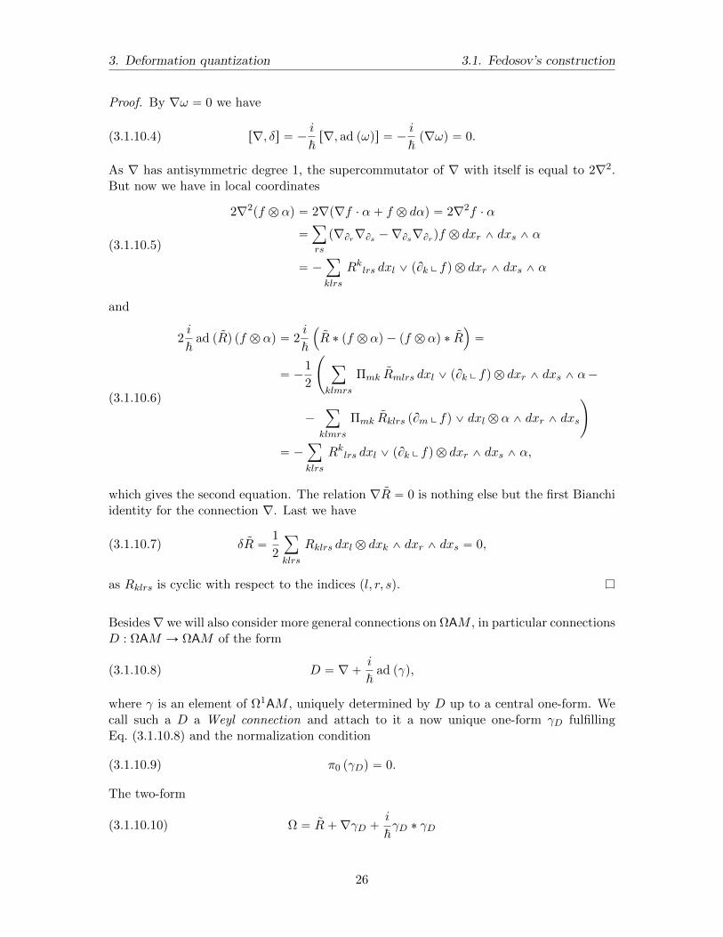
3. Deformation quantization 3.1. Fedosov’s construction
Proof. By ∇ω “ 0 we have
(3.1.10.4) r∇, δs “ ´ i~r∇, ad pωqs “ ´
i
~p∇ωq “ 0.
As ∇ has antisymmetric degree 1, the supercommutator of ∇ with itself is equal to 2∇2.But now we have in local coordinates
2∇2pf b αq “ 2∇p∇f ¨ α` f b dαq “ 2∇2f ¨ α
“ÿ
rs
p∇Br∇Bs ´∇Bs∇Brqf b dxr ^ dxs ^ α
“ ´ÿ
klrs
Rklrs dxl _ pBk x fq b dxr ^ dxs ^ α
(3.1.10.5)
and
2i
~ad pRq pf b αq “ 2
i
~
´
R ˚ pf b αq ´ pf b αq ˚ R¯
“
“ ´1
2
˜
ÿ
klmrs
Πmk Rmlrs dxl _ pBk x fq b dxr ^ dxs ^ α´
´ÿ
klmrs
Πmk Rklrs pBm x fq _ dxl b α^ dxr ^ dxs
¸
“ ´ÿ
klrs
Rklrs dxl _ pBk x fq b dxr ^ dxs ^ α,
(3.1.10.6)
which gives the second equation. The relation ∇R “ 0 is nothing else but the first Bianchiidentity for the connection ∇. Last we have
(3.1.10.7) δR “1
2
ÿ
klrs
Rklrs dxl b dxk ^ dxr ^ dxs “ 0,
as Rklrs is cyclic with respect to the indices pl, r, sq.
Besides∇ we will also consider more general connections on ΩAM , in particular connectionsD : ΩAM Ñ ΩAM of the form
(3.1.10.8) D “ ∇` i
~ad pγq,
where γ is an element of Ω1AM , uniquely determined by D up to a central one-form. Wecall such a D a Weyl connection and attach to it a now unique one-form γD fulfillingEq. (3.1.10.8) and the normalization condition
(3.1.10.9) π0 pγDq “ 0.
The two-form
(3.1.10.10) Ω “ R`∇γD `i
~γD ˚ γD
26
3. Deformation quantization 3.1. Fedosov’s construction
will then be called the Weyl curvature of D. Furthermore a Weyl connection D will becalled abelian, if its Weyl curvature is a central form or, using the following proposition,if
(3.1.10.11) D2 “i
~ad pΩq “ 0.
3.1.11 Proposition Let D be a Weyl connection on ΩAM and Ω its Weyl curvature.Then Ω fulfills the Bianchi-identity
(3.1.11.1) DΩ “ 0
and the relation
(3.1.11.2) D2 “i
~ad pΩq.
Proof. The Bianchi-identity follows from
DΩ “ ∇Ω`i
~rγD,Ωs “
“ ∇R`∇2γD `i
~r∇γD, γDs `
i
~rγD, Rs `
i
~rγD,∇γDs `
i
~rγD, γ
2Ds.
(3.1.11.3)
By the Bianchi identity for ∇ the first term vanishes, the last one as γD commutes withγ2D. By Eq. (3.1.10.2) the second and the fourth term cancel each other, hence DΩ “ 0.
Using Proposition 3.1.10 the second equation follows immediately:
D2 “ ∇2 `i
~ad p∇γDq `
1
2
ˆ
i
~
˙2
ad prγD, γDsq
“i
~ad
ˆ
R`∇γD `i
~γD ˚ γD
˙
.
(3.1.11.4)
We now will look for Abelian D or in other words for conditions on γD which guarantee Dto be Abelian. To achieve this let us write γD in the form
(3.1.11.5) γD “ ω ` r,
where r P Ω1AM . Then we have
(3.1.11.6) Ω “ R`∇r ` i
~r ˚ r `
i
~ad pωqprq ´ 1b ω,
as ω ˚ ω “ i~ 1b ω. If now r fulfills
(3.1.11.7) δprq “ R`∇r ` i
~r ˚ r,
then Ω “ ´1b ω, hence D will be Abelian.
27

3. Deformation quantization 3.1. Fedosov’s construction
3.1.12 Lemma An element r P Ω1AM with degF r ě 2 fulfills δ´r “ 0 and Eq. (3.1.11.7)if and only if
(3.1.12.1) r “ δ´R` δ´ˆ
∇r ` i
~r ˚ r
˙
.
Proof. If the first condition is satisfied, (3.1.12.1) follows easily from pδ´δ ` δδ´qr “ r.Let us show the converse and suppose (3.1.12.1) to be true. Then obviously δ´r “ 0 bypδ´q2 “ 0. Let D be the Weyl connection on ΩAM with γD “ ω ` r. To prove (3.1.11.7)it then suffices to show Ω “ ´1b ω. We have
(3.1.12.2) δ´pΩ` 1b ωq “ δ´ˆ
R`∇r ` i
~r ˚ r
˙
´ δ´δr “ r ´ δ´δr “ δδ´r “ 0,
hence by the Bianchi identity DΩ “ 0 and Dp1b ωq “ 1b dω “ 0 the relation
(3.1.12.3) δpΩ` 1b ωq “ pD ` δqpΩ` 1b ωq
is true. Using the Hodge-deRham decomposition in ΩAM this entails
(3.1.12.4) Ω` 1b ω “ δ´pD ` δqpΩ` 1b ωq “ δ´ˆ
∇` i
~ad prq
˙
pΩ` 1b ωq.
As the operator δ´`
∇` i~ ad prq
˘
raises the F-degree by 1, we must have Ω` 1b ω “ 0.But this gives the claim.
28

4. Molecular quantum mechanics
4.1. The von Neumann–Wigner no-crossing rule
4.1.1 Theorem (von Neumann & Wigner (1929)) For any positive integer n let
Hermpnq “
A P glpn,Cq | A˚ “ A(
be the space of all (complex) hermitian nˆ n matrices and
Sympnq “
A P glpn,Rq | At “ A(
the space of all (real) symmetric nˆn matrices. Then Hermpnq and Sympnq are real vector
space of dimension n2 and npn`1q2 , respectively. The subspaces Hermdgtpnq Ă Hermpnq and
Symdgtpnq Ă Sympnq of hermitian respectively symmetric n ˆ n matrices having at leastone degenerate eigenvalue are (real) algebraic varieties of codimension 3 and 2, respectively.
4.1.2 Remark Recall that an eigenvalue of a real or complex n ˆ n matrix is calleddegenerate if its algebraic multiplicity is at least 2. For hermitian or symmetric matricesthis is equivalent to the geometric multiplicity of the eigenvalue being ě 2.
Proof. Since the diagonal elements of a hermitian matrix A “ paijq1ďi,jďn are all real andaij “ aji for i ‰ j, the (real) dimension of Hermpnq is given as the sum of the numberof diagonal elements of A and twice the number of its upper diagonal elements. So oneobtains
dimHermpnq “ n` 2n´1ÿ
k“1
k “ n` pn´ 1qn “ n2 .
In the real symmetric case, one needs to count the number of diagonal or upper diagonalelements, hence
dimSympnq “nÿ
k“1
k “npn` 1q
2.
The eigenvalues of a complex hermitian or real symmetric matrix A coincide with thezeros of its characteristic polynomial χA “ detpA ´ λInq P Crλs. Let discriminantepχAqbe the discriminant of the characteristic polynomial; see (Cohen, 1993, Sec. 3.3.2) for thedefinition and properties of the discriminant. Then discriminantepχAq is a polynomial in thecoefficients of χA and vanishes if and only if χA has a multiple root. Since the coefficients ofχA are polynomials in the entries of A, the set of hermitian (respectively symmetric) nˆnmatrices with a degenerate eigenvalue is a real algebraic variety in Hermpnq (respectivelySympnq).
29

4. Molecular quantum mechanics 4.1. The von Neumann–Wigner no-crossing rule
Next let us determine the codimension of the variety Hermdgtpnq. To this end recall that ahermitian matrix A can be written in the form A “ UDU´1, where D is a diagonal matrixhaving the eigenvalues of A as its entries and where U is a complex unitary nˆ n matrix.The diagonal matrix D “ pdijq1ďi,jďn is uniquely determined when one requires that itsdiagonal entries are linearly ordered so that d11 ď . . . ď dnn. The matrix U is uniquely upto a unitary matrix V commuting with D. In case A has n different eigenvalues, the onlyunitary matrices commuting with D are diagonal matrices with entries from Up1q. SincedimUpnq “ n2 Hence the codimension of Hermdgtpnq in Hermpnq is
30

Part III.
Quantum Field Theory
31

5. Axiomatic quantum field theory a laWightman and Garding
5.1. Wightman axioms
5.1.1 The Wightman axioms were first introduced in the paper Wightman & Garding(1964), and then explained in more detail in the textbooks Jost (1965) and (Streater &Wightman, 2000, Sec. 3.1). The latter is still the main reference for the axiomatic treatmentof quantum field theory in the spirit of Wightman and Garding. See also (Schottenloher,2008, Sec. 8.3) for a more modern formulation which we follow here.
5.1.2 Definition A Wightman quantum field theory of space-time dimension d`1, whered P Ną0, consists of the following data:
• the state space of the theory given by the projective space PpHq associated to aseparable complex Hilbert space H,
• a distinguished state ω˝ “ Cv˝ P PpHq called the vacuum state together with thechoice of a normalized representing vector v˝ P H called vacuum vector,
• a unitary representation U :Ă
PÒ`pd` 1q Ñ UpHq of the universal cover
Ă
PÒ`pd` 1q – Rd`1 ¸ĄSOÒp1, dq
of the proper orthochronous Poincare group PÒ`pd` 1q “ R1`d ¸ SOÒp1, dq,
• and finally a family pΦjq1ďjďn, n P Ną0, of so-called field operators
Φj : SpRd`1q Ñ LupHq
which are defined on the Schwartz space of rapidly decreasing functions on Rn andmap to the space of unbounded linear operators on the Hilbert space H.
These data are assumed to fulfill the following axioms, the so-called Wightman axioms:
(W1) (Assumptions about the domain and the continuity of the field)There exists a dense linear subspace D Ă H containing v˝ such that D is contained inthe domain of all the operators Φjpfq and their adjoints Φjpfq˚, where f P SpRd`1q
and j “ 1, . . . , k. Moreover, the unitary representation U and the operators Φjpfqand Φjpfq˚ leave D invariant that is
Upa,AqD Ă D, ΦjpfqD Ă D, Φjpfq˚D Ă D
32

5. Axiomatic quantum field theory a la Wightman and Garding 5.1. Wightman axioms
for all pa,Aq PĂ
PÒ`p1, dq, f P SpRd`1q and j “ 1, . . . , k. Finally, for every v P D,w P H and j “ 1, . . . , n the maps
SpRd`1q Ñ C, f ÞÑ xw,Φjpfqvy
are tempered distributions.
(W2) (Transformation law of the field)
For all pa,Aq PĂ
PÒ`pd` 1q and all f P SpRd`1q the equation
Upa,AqΦjpfqUpa,Aq´1 “
nÿ
k“1
%jk`
A´1˘
Φkppa,Aqfq
is valid over the domain D, where % : ĄSOÒp1, dq Ñ GLpn,Cq is a finite dimensionalrepresentation of the universal cover of the proper orthochronous Lorentz groupSOÒp1, dq and the action of rPpd` 1q on SpRd`1q is given by
rPpd` 1q ˆ SpRd`1q Ñ SpRd`1q,`
pa,Aq, f˘
ÞÑ pa,Aqf “´
Rd`1 Q x ÞÑ f`
A´1px´ aq˘
P C¯
.
(W3) (Local commutativity or microscopic causality)If the support of test functions f, g P SpRd`1q is space-like separated that is iffpxq gpyq “ 0 for all x, y P Rd`1 with xx´ y, x´ yyM ě 0, then for all j, k “ 1, . . . , nthe relation
rΦjpfq,Φkpgqs´ “ rΦjpfq,Φjpgq˚s´ “ 0
or the relationrΦjpfq,Φkpgqs` “ rΦ
jpfq,Φjpgq˚s` “ 0
holds true over the domain D. Hereby, rS, T s´ denotes the commutator
rS, T s´ : DÑ H, v ÞÑ STv ´ TSv
and rS, T s` the anti-commutator
rS, T s` : DÑ H, v ÞÑ STv ` TSv
of two operators S, T P LupHq which are both assumed to be defined on the domainD and to leave it invariant.
(W4) (Cyclicity of the vacuum vector)The linear span of the set of all elements v P H of the form
v “ Φj1pf1q . . . Φjmpfmqv˝ ,
where m P N, 1 ď j1, . . . , jm ď n, and f1, . . . , fm P SpRd`1q, is dense in H.
33

5. Axiomatic quantum field theory a la Wightman and Garding 5.2. Fock space
5.1.3 Remarks (a) The vacuum vector v˝ being normalized just means that v˝ “ 1.This implies that the vacuum state ω˝ determines v˝ only up to a factor z P S1 Ă C.The physically measurable quantities of the quantum field theory such as expectationvalues or transition amplitudes do not depend on that choice.
(b) The field operators Φj are operator valued distributions. This reflects the fact thatonly the “smeared” fields Φjpfq can be interpreted physically as observable. Thenotation Φjpxq for a field evaluated at a space-time point x P R1,3 therefore does notmake sense, neither mathematically nor physically. Nevertheless it is often used forreasons of convenience, in particular in the physics literature. The smeared field Φjpfqthen is interpreted, again imprecisely, as the integral
Φjpfq “
ż
Rd`1
fpxqΦjpxq dx .
We will avoid the notation of pointwise evaluated fields in the formulation of definitionsand theorems, but occasionally use it as a heuristic.
For example, Axiom (W3) can heuristically be interpreted as saying that the (anti-)commutation relations
rΦjpxq,Φkpyqs¯ “ rΦjpxq,Φjpyq˚s¯ “ 0
hold true for x, y P R1,d space-like separated which means for the situation when
xx´ y, x´ yyM ă 0 .
5.2. Fock space
5.2.1 Recall that the Hilbert tensor product H1pbH2 of two Hilbert spaces H1 and H2 isdefined as the completion of the the algebraic tensor product H1bH2 with inner product
x¨, ¨y :`
H1 bH2
˘
ˆ`
H1 bH2
˘
Ñ K,`
v1 b v2, w1 b w2
˘
ÞÑ xv1, w1y ¨ xv2, w2y .
The norm of v1 b v2 P H1pbH2 is then given by v1 b v2 “ v1 ¨ v2, and every elementv P H1pbH2 can be written as the sum of a square summable family
`
vi1 b vi2˘
iPIthat is
asv “
ÿ
iPI
vi1 b vi2 where v2 “ÿ
iPI
vi12 ¨ vi2
2 ă 8 .
If peiqiPI is Hilbert basis for H1 and pfjqjPJ one of H2, the family peibfjqpi,jqPIˆJ is a Hilbert
basis of H1pbH2. Moreover, the canonical map ι : H1 ˆH2 Ñ H1pbH2, pv1, v2q ÞÑ v1 b v2 isbilinear and weakly Hilbert–Schmidt that means that there exists a C ě 0 such that forall Hilbert bases peiqiPI of H1, all Hilbert bases pfjqjPJ of H2, and all w P H1pbH2
ÿ
pi,jqPIˆJ
|xιpei, fjq, wy|2ď Cw2 .
Note that if this condition holds for one Hilbert basis of H1 and one of H2, it holds for all.The Hilbert tensor product, which in the following we will only call tensor product, nowsatsifies the following universal property:
34

5. Axiomatic quantum field theory a la Wightman and Garding 5.2. Fock space
(HTensor) For every Hilbert space H and every weakly Hilbert–Schmidt bilinear map µ :H1 ˆ H2 Ñ H there exists a unique bounded linear map M : H1pbH2 Ñ H suchthat the diagram
H1 ˆH2 H
H1pbH2
ι
µ
M
commutes.
For a proof of the universal property see ?.
The universal property of the Hilbert tensor product entails several categorical properties.First, the Hilbert tensor product is a functor in each argument which means that forbounded linear maps Ai : Hi Ñ Ki, i “ 1, 2, between Hilbert spaces one has a boundedlinear map A1pbA2 : H1pbH2 Ñ K1pbK2 such that idH1
pbidH2 “ idH1 pbH2and such that
pB1pbB2q ˝ pA1pbA2q “ pB1 ˝A1qpbpB2 ˝A2q for bounded linear maps Bi : Ki Ñ Li, i “ 1, 2,between Hilbert spaces and Ai, i “ 1, 2, as before. Second, for every Hilbert space H onehas two natural isomorphisms
uH : KpbH Ñ H, z b v Ñ zv and Hu : HpbKÑ H, v b z Ñ zv
called the left and right unit, respectively. Third, for every tripe of Hilbert spaces H,K,Lthere is a natural isomorphism, called associator
aH,K,L : pHpbKqpbL Ñ HpbpKpbLq .
These data fulfill the so-called coherence conditions that is the pentagon diagram
and the triangle diagram
pHpbKqpbL HpbpKpbLq
HpbL
aH,K,L
HupbidL idH pbuL
commute for all Hilbert spaces H,K,L,M.
5.2.2 Now let us fix a Hilbert space H and consider the higher Hilbert tensor productpowers Hpbn for natural n defined recursively by
Hpb 0 “ K, H
pbn`1 “ H pb`
Hpbn
˘
.
35

Part IV.
Mathematical Toolbox
36

6. Topological Vector Spaces
6.1. Seminorms, locally convex topologies, and convergence
6.1.1 Throughout this chapter the symbol K will always stand for the field of real numbersR or the field of complex numbers C.
6.1.2 Definition Let V be K-vector space. By a seminorm on V one then understands amap p : V Ñ Rě0 with the following properties:
(N1) The map p is absolutely homogeneous that means
pprvq “ |r| ppvq for all v P V and r P K.
(N2) The map p is subadditive or in other words satisfies the triangle inequality
ppv ` wq ď ppvq ` ppwq for all v, w P V.
A seminorm is called a norm if in addition the following axiom is satisfied:
(N3) For all v P V the relation ppvq “ 0 holds true if and only if v “ 0.
A K-vector space V together with a norm ¨ : V Ñ Rě0, v ÞÑ v is called a normedvector space.
If p is a seminorm on V we denote for every v P V and ε ą 0 by Bp,εpvq the (open) ε-ballassociated with p and with center v that is the set
Bp,εpvq “
w P Vˇ
ˇ ppw ´ vq ă ε(
.
The closed ε-ball associated with p and with center v is defined as
Bp,εpvq “
w P Vˇ
ˇ ppw ´ vq ď ε(
.
The positive number ε is sometimes called the radius of the ball. When by the context itis clear which seminorm p a ball is associated with we often do not mention p explicitely.This is in particular the case when the underlying vector space is a normed vector space.For the particular radius 1 we denote the corresponding balls by Bppvq and Bppvq andcall them the open respectively closed unit balls. If P is a finite set or a finite family ofseminorms on V we define the open and closed ε-multiballs with center v by
BP,εpvq “
w P Vˇ
ˇ ppw ´ vq ă ε for all p P P(
andBP,εpvq “
w P Vˇ
ˇ ppw ´ vq ď ε for all p P P(
,
respectively.
37

6. Topological Vector Spaces 6.1. Seminorms, locally convex topologies, and convergence
6.1.3 Definition A subset C of a K-vector space V is called
(1) convex if tv ` p1´ tqw P C for all v, w P C and t P r0, 1s,
(2) absolutely convex if tv ` sw P C for all v, w P C and t, s P K such that |t| ` |s| ď 1,
(3) symmetric if ´v P C for all v P C,
(4) circled or balanced if tv P C for all v P C and t P K with |t| ď 1,
(5) absorbing or absorbant if for every v P V there exists a real positive number t0 suchthat v P tC for all t P K with |t| ě t0,
(6) and, finally, a cone if tv P C for all v P C and t P r0, 1s.
6.1.4 Lemma A subset C of a K-vector space V is absolutely convex if and only if it iscircled and convex.
Proof.
6.1.5 Proposition Let V be a K-vector space, and P a finite set of seminorms on V.Then, for every ε ą 0 and v P V , the ε-multiballs BP,εpvq and BP,εpvq are convex and theε-multiballs BP,εp0q and BP,εp0q are absolutely convex and absorbant.
Proof. Axiom (N1) immediately entails that BP,εp0q and BP,εp0q are circled. Axiom (N2)together with (N1) entails that the sets BP,εpvq and BP,εpvq are convex. Namely, if w1, w2 P
BP,εpvq and t P r0, 1s, then one has for all seminorms p P P
p ptw1 ` p1´ tqw2 ´ vq ď t p pw1 ´ vq ` p1´ tq pw2 ´ vq ă t ε` p1´ tq ε “ ε
and likewise p ptw1 ` p1´ tqw2 ´ vq ď ε for all w1, w2 P BP,εpvq and p P P .
Now let v P V and ε ą 0 be given. Put tp “ppvq`1
ε for every p P P and t0 “ maxttp | p P P u.Then one has for all t P K with |t| ě t0
p
ˆ
1
tv
˙
ďε
ppvq ` 1ppvq ă ε ,
hence v P tBP,εpvq. So BP,εpvq is absorbing. Since BP,εpvq contains the absorbing setBP,εpvq it is absorbing as well.
6.1.6 Assume to be given a family P “ ppiqiPI of seminorms on a vector space E. Let FpP qbe the collection of all finite subfamilies of P that is of all families of seminorms the formQ “ ppjqjPJ where J Ă I is finite. A topological base on E is then given by the set
BP “
BQ,εpvqˇ
ˇ Q P FpP q, v P E, ε ą 0(
.
The topology generated by this base is denoted OP and called the topology defined by thefamily of seminorms P .
It has the following properties:
38
6. Topological Vector Spaces 6.2. Function spaces and their topologies
(TVS1) Addition ` : Eˆ E Ñ E is continuous.
(TVS2) Multiplication by scalars ¨ : Kˆ E Ñ E is continuous.
(TVS3) The topology on E has a base consisting of convex sets.
Proof. We prove continuity of addition first. Let v1, v2 P E, Q P FpP q, and ε ą 0. Sincethe triangle inequality holds for every seminorm in F , one has
BQ, ε2pv1q `BQ, ε
2pv2q Ă BQ,εpv1 ` v2q ,
which entails continuity of addition at each pv1v2q P E ˆ E. Next consider multiplicationby scalars and let λ P K and v P E. Again let Q “ ppjqjPJ P FpP q and ε ą 0. LetC1 “ suptpjpvq | j P Ju ` 1 and C2 “ |λ| ` 1 and put δ1 “ mint1, ε
2C1u and δ2 “
ε2C2
.Then one obtains by absolute homogeneity and subadditivity of each seminorm
pjpµw ´ λvq ď |µ| pjpw ´ vq ` |µ´ λ| pjpvq for all λ P K and w P E,
henceBδ1pλq ¨BQ,δ2pvq Ă BQ,εpλ ¨ vq ,
where Bδ1pλq “ tµ P K | |µ ´ λ| ă δ1u. This shows continuity of scalar multiplication ateach pλ, vq P Kˆ E.
Since each of the base elements BQ,εpvq P BP is convex by the preceding proposition,Axiom (TVS3) holds true as well.
6.1.7 Definition A vector space E over the field K together with a topology O such thatAxioms (TVS1) and (TVS2) are fulfilled is called a topological vector space, for short a TVS.If in addition Axiom (TVS3) holds true, then pE,Oq is called a locally convex topologicalvector space.
6.1.8 As we have seen already, any vector space with a topology defined by a family ofseminorms on it is a locally convex TVS. The converse also holds true which we will showin the following.
6.2. Function spaces and their topologies
6.2.1 Proposition Let X be a topological space. Then the algebra
CbpX,Kq “
f P CpX,Kqˇ
ˇ DC ą 0@x P X : |fpxq| ď C(
of bounded continuous K-valued functions on X together with the supremums-norm
¨ 8 : CbpX,Kq Ñ K, f ÞÑ sup
|fpxq|ˇ
ˇ x P X(
is a Banach algebra. This means in particular that for X compact the algebra CpX,Kqendowed with the norm ¨ 8 is a Banach algebra.
Proof.
39

6. Topological Vector Spaces 6.3. Summability
6.3. Summability
6.3.1 Assume to be given a locally convex t.v.s. E over the field K of real or complexnumbers. Let pviqiPI be a family of elements of E. Let FpIq be the set of finite subsets ofI and note that it is directed by set-theoretic inclusion. The family pviqiPI then gives rise
to the net´
ř
iPJ vi
¯
JPFpIq. One calls the family pviqiPI summable to an element v P E if
the net´
ř
iPJ vi
¯
JPFpIqconverges to v. In other words this means that for every convex
zero neighborhood U Ă E and ε ą 0 there exists a finite subset JU,ε Ă I such that for allfinite sets J with JU,ε Ă J Ă I
pU
˜
v ´ÿ
iPJ
vi
¸
ă ε .
If E is Hausdorff, the limit v of a summable family pviqiPI is uniquely determined, and onewrites in this situation
v “ÿ
iPI
vi .
We denote the space of summable families in E over the given index set I by `1pI,Eq.
Besides summability the notions of absolute, weak, and total summability have been intro-duced in the functional analysis literature, where they are used in the study of topologicaltensor products and nuclearity of locally convex topological vector spaces, cf. Grothendieck(1955); Pietsch (1972). Let us explain what these further notions of summability mean.Like before let pviqiPI be a family of elements of the locally convex t.v.s. E.
A family pviqiPI of elements of E is called weakly summable to v P E if for every continuous
linear form α : E Ñ K the net´
ř
iPJ αpviq¯
JPFpIqconverges in K to αpvq. In other words
this means that for every α P E1 and ε ą 0 there exists a finite set Jα,ε Ă I such that forall finite sets J with Jα,ε Ă J Ă I
ˇ
ˇ
ˇ
ˇ
ˇ
αpvq ´ÿ
jPJ
αpviq
ˇ
ˇ
ˇ
ˇ
ˇ
ă ε .
The set of all weakly summable families in E with index set I is denoted `1rI,Es.
If for every convex zero neighborhood U Ă Eÿ
iPI
pU pviq ă 8 ,
then the family pviqiPI is called absolutely summable. We denote the set of all absolutelysummable families pviqiPI in E by `1tI,Eu.
Finally, a family pviqiPI in E is called totally summable if there exists a bounded subsetB Ă E such that
ÿ
iPI
pB pviq ă 8 .
Note that this implies that
40

7. Distributions and Fourier transform
7.1. Schwartz test functions
41

8. Hilbert Spaces
8.1. Inner product spaces
8.1.1 Let us first remind the reader that as before K stands for the field of real or of complexnumbers. We will keep this notational agreement throughout the whole chapter.
8.1.2 Definition By a sesquilinear form on a K-vector space V one understands a mapx¨, ¨y : V ˆV Ñ K with the following two properties:
(SF1) The map x¨, ¨y is linear in its first coordinate which means that
xv1 ` v2, wy “ xv1, wy ` xv2, wy and xrv, wy “ rxv, wy
for all v, w, v1, v2 P V and r P K.
(SF2) The map x¨, ¨y is conjugate-linear in its second coordinate which means that
xv1 ` v2, wy “ xv1, wy ` xv2, wy and xv, rwy “ rxv, wy
for all v, w, v1, v2 P V and r P K.
A hermitian form is a sesquilinear form x¨, ¨y on V with the following additional property:
(SF3) The map x¨, ¨y is conjugate symmetric which means that
xv, wy “ xw, vy for all v, w P V .
A sesquilinear form x¨, ¨y is called weakly-nondegenerate if it satisfies axiom
(SF4w) For every v P V, the map V Ñ K, w Ñ xw, vy is the zero map if and only if v “ 0.
Finally, one calls a hermitian form x¨, ¨y on V positive semidefinite if
(SF5s) xv, vy ě 0 for all v P V.
8.1.3 Remark Recall that a map x¨, ¨y : V ˆV Ñ K is called bilinear, if it satisfies (SF1)and
(BF1) The map x¨, ¨y is linear in its second coordinate which means that
xv1 ` v2, wy “ xv1, wy ` xv2, wy and xv, rwy “ rxv, wy
for all v, v1, v2, w P V and r P K.
42

8. Hilbert Spaces 8.1. Inner product spaces
If the underlying ground field K coincides with the field of real numbers, a sesquilinearform is by definition the same as a bilinear form, and a hermitian form the same as asymmetric bilinear form.
8.1.4 Given a positive semidefinite hermitian form x¨, ¨y on a K-vector space V, one callstwo vectors v, w P V orthogonal if xv, wy “ 0. Since the hermitian form x¨, ¨y is assumed tobe positive semidefinite, the map
¨ : V Ñ Rě0, v ÞÑ v “a
xv, vy
is well-defined. We will later see that ¨ is a seminorm on V and therefore call the map ¨ the seminorm associated to x¨, ¨y. The following formulas are immediate consequencesof the properties defining a positive semidefinite hermitian form and the definition of theassociated seminorm:
v ` w2 “ v2 ` 2Re xv, wy ` w2 for all v, w P V ,(8.1.4.1)
v ` w2 “ v2 ` w2 for all orthogonal v, w P V ,(8.1.4.2)
v ` w2 ` v ´ w2 “ 2`
v2 ` w2˘
for all v, w P V ,(8.1.4.3)
rv “a
|r|2xv, vy “ |r|v for all v, w P V and r P K .(8.1.4.4)
Formula (8.1.4.2) is an abstract version of the pythagorean theorem, Equation (8.1.4.3) iscalled the parallelogram identity. The triangle inequality for the map ¨ will turn out tobe a consequence of the following result.
8.1.5 Proposition (Cauchy–Schwartz inequality) Given a positive semidefinite her-mitian form x¨, ¨y on a K-vector space V the following inequality holds true:
(8.1.5.1) |xv, wy| ď vw for all v, w P V.
Equality holds if and only if v and w are linearly dependant.
Proof. If v or w is 0, the proof is trivial, hence we can assume both to be nonzero. Put
c “ ´xv, wy
v2
and compute
0 ď cv ` w2 “ xcv ` w, cv ` wy “ |c|2xv, vy ` cxv, wy ` cxw, vy ` xw,wy “
“ |c|2v2 ` 2Re`
cxv, wy˘
` w2 “|xv, wy|2
v2´ 2
|xv, wy|2
v2` w2 “
“ w2 ´|xv, wy|2
v2.
(8.1.5.2)
Hence|xv, wy|2 ď v2w2
which entails the Cauchy–Schwartz inequality.
43

8. Hilbert Spaces 8.1. Inner product spaces
If v, w are linearly dependant nonzero elements of V, then there exists a nonzero scalara P K such that v “ aw. Hence
|xv, wy| “ |a| w2 “ vw .
Vice versa, if equality holds, then Equation (8.1.5.2) entails that cv`w “ 0, which meansthat v and w are linearly dependant.
8.1.6 Lemma A positive semidefinite hermitian form x¨, ¨y on a K-vector space V isweakly-nondegenerate if and only if it is positive definite that is if and only if
(SF5p) xv, vy ą 0 for all v P Vzt0u.
Proof. A positive definite real bilinear or complex hermitian form x¨, ¨y is non-degeneratesince for every v P Vzt0u the linear form x´, vy : V Ñ K then is nonzero because xv, vy ą 0.
Conversely, if x´, vy : V Ñ K is nonzero for all v P Vzt0u, then there exists an elementw P V such that xw, vy ‰ 0. The Cauchy–Schwarz inequality entails
0 ă |xw, vy|2 ď xw,wy xv, vy ,
which implies xv, vy ą 0. Hence x¨, ¨y is positive definite.
8.1.7 Proposition The map
¨ : V Ñ Rě0, v ÞÑ v “a
xv, vy
associated to a positive semidefinite hermitian form x¨, ¨y on a K-vector space V is a semi-norm. If the hermitian form is positive definite, then ¨ is even a norm.
Proof. Absolute homogeneity (N1) is given by Eq. (8.1.4.4). The triangle inequality is aconsequence of the Cauchy–Schwarz inequality:
v ` w2 “ v2 ` 2Re xv, wy ` w2 ď v2 ` 2 v w ` w2 “`
v ` w˘2.
Finally, if x¨, ¨y is positive definite, then v “a
xv, vy ą 0 for all v P Vzt0u, so ¨ is anorm.
8.1.8 Definition By an inner product or a scalar product on a K-vector space H oneunderstands a positive definite hermitian form on H. A K-vector space H together with aninner product x¨, ¨y : HˆH Ñ K is called an inner product space or a pre-Hilbert space.
A hermitian form on a K-vector space H which is only positive semidefinite is called asemi-inner product or a semi-scalar product.
A Hilbert space is an inner product space pH, x¨, ¨yq which is complete as a normed vectorspace. In other words, a Hilbert space is Banach space where the norm on the space isinduced by an inner product.
44

8. Hilbert Spaces 8.1. Inner product spaces
8.1.9 Examples 1. The vector space Rn with the euclidean inner product
x¨, ¨y : Rn ˆ Rn Ñ R,`
pv1, . . . , vnq, pw1, . . . , wnq˘
ÞÑ
nÿ
i“1
viwi
is a real inner product space.
2. The vector space Cn together with the hermitian form
x¨, ¨y : Cn ˆ Cn Ñ C,`
pv1, . . . , vnq, pw1, . . . , wnq˘
ÞÑ
nÿ
i“1
viwi
is a complex inner product space.
3. Let
L2pRnq “"
f : Rn Ñ Cˇ
ˇ
ˇ
ˇ
f is Lebesgue measurable and
ż
Rn|f |2dλ ă 8
*
denote the space of Lebesgue square integrable functions on Rn. Then the map
x¨, ¨y : L2pRnq ˆ L2pRnq Ñ C, pf, gq ÞÑż
Rnfg dλ
is a positive semidefinite hermitian form on L2pRnq. Modding out L2pRnq by thekernel
N :“ Kerp ¨ q “
"
f P L2pRnqˇ
ˇ
ˇ
ˇ
ż
Rn|f |2dλ “ 0
*
gives the Lebesgue spaceL2pRnq :“ L2pRnqN .
The hermitian form x¨, ¨y vanishes on N ˆ L2pRnq and L2pRnq ˆ N by the Cauchy–Schwarz inequality, hence descends to a hermitian form
x¨, ¨y : L2pRnq ˆ L2pRnq Ñ C, pf `N, g `Nq ÞÑ
ż
Rnfg dλ .
That hermitian form is positive definite, since xf`N, f`Ny “ 0 meansş
Rn |f |2dλ “ 0,
hence f P N. So L2pRnq together with x¨, ¨y is a Hilbert space which we call the Hilbertspace of square-integrable functions on Rn.
4. The set
`2 “
#
pzkqkPN P CN
ˇ
ˇ
ˇ
ˇ
ˇ
8ÿ
k“1
|zk|2 ă 8
+
of square summable sums of complex numbers is a complex inner product space withinner product
x¨, ¨y : `2 ˆ `2 Ñ C,`
pzkqkPN, pwkqkPN˘
ÞÑ
8ÿ
k“1
zkwk
45

8. Hilbert Spaces 8.1. Inner product spaces
8.1.10 Theorem Let H be a normed K-vector space. Then the norm ¨ : H Ñ Rě0 isassociated to an inner product x¨, ¨y : HˆH Ñ K if and only if the parallelogram identity
v ` w2 ` v ´ w2 “ 2v2 ` 2w2
holds true for all v, w P H. In this case, the inner product of two elements v, w P V can beexpressed by the polarization identity for K “ R
(8.1.10.1) xv, wy “1
4
`
v ` w2 ´ v ´ w2˘
“1
2
`
v ` w2 ´ v2 ´ w2˘
respectively by the polarization identity for K “ C
(8.1.10.2) xv, wy “1
4
4ÿ
k“1
ik v ` ik w2 .
Proof. The forward direction is a consequence of 8.1.4, Eq. 8.1.4.3. To show the backwarddirection we consider two cases K “ R and K “ C separately.
1. Case. Given the norm ¨ define x¨, ¨y : V ˆV Ñ R by real polarization
xv, wy “1
4
`
v ` w2 ´ v ´ w2˘
, where v, w P V .
Note that the parallelogram identity entails
1
4
`
v ` w2 ´ v ´ w2˘
“1
2
`
v ` w2 ´ v2 ´ w2˘
.
Observe that by definition xv, wy “ xw, vy and v “a
xv, vy. Let us show additivity inthe first variable. Let v1, v2, w P V and compute using the parallelogram identity
v1 ` v2 ` w2 “ 2v1 ` w
2 ` 2v22 ´ v1 ` w ´ v2
2 ,
v1 ` v2 ` w2 “ 2v2 ` w
2 ` 2v12 ´ v2 ` w ´ v1
2 .
Hence
v1 ` v2 ˘ w2 “ v1 ˘ w
2 ` v2 ˘ w2 ` v1
2 ` v22 ´ v1 ˘ w ´ v2
2 ´ v2 ˘ w ´ v12 .
Subtracting the ´ version from the ` version of this equation entails
xv1 ` v2, wy “1
4
`
v1 ` v2 ` w2 ´ v1 ` v2 ´ w
2˘
“
“1
4
`
v1 ` w2 ` v2 ` w
2 ´ v1 ´ w2 ´ v2 ´ w
2˘
“ xv1, wy ` xv2, wy ,
so additivity in the first variable is proved. By induction one derives from this that for allnatural n
(8.1.10.3) xnv,wy “ nxv, wy for all v, w P V .
46

8. Hilbert Spaces 8.1. Inner product spaces
Since then x´nv,wy ´ nxv, wy “ x´nv ` nv,wy “ 0 for all n P N, Eq. (8.1.10.3) also holdsfor n P Z. Now let p P Z and q P Ną0. Then q xpqv, wy “ xpv, wy “ p xv, wy, hence one hasfor rational r
(8.1.10.4) xrv, wy “ rxv, wy for all v, w P V .
Since addition, multiplication by scalars and the norm are continuous, the function
RÑ R, r ÞÑ xrv, wy ´ rxv, wy “1
4
`
rv ` w2 ` rv ´ w2 ´ rv ´ w2 ´ rv ` w2˘
is continuous. Since it vanishes over Q, it has to coincide with the zero map. Therefore,Eq. (8.1.10.4) holds for all r P R. So x¨, ¨y is linear in the first coordinate. By symmetry, itis so too in the second coordinate. Hence x¨, ¨y is a symmetric bilinear form inducing ¨ .
2. Case. In the case K “ C use complex polarization and put
xv, wy “1
4
4ÿ
k“1
ik v ` ik w2 for all v, w P V .
Then x¨, ¨y is conjugate symmetric, since
xv, wy “1
4
4ÿ
k“1
p´iqk v ` ik w2 “1
4
4ÿ
k“1
p´iqk p´iqk v ` w2 “ xw, vy .
Next compute
Rexv, wy “1
4
`
v ` w2 ´ v ´ w2˘
and
Imxv, wy “1
4
`
v ` iw2 ´ v ´ iw2˘
.
By the first case one concludes that Rex¨, ¨y and Imx¨, ¨y are both R-linear in the first andthe second coordinate. Moreover,
Rexiv, wy “1
4
`
iv ` w2 ´ iv ´ w2˘
“1
4
`
v ´ iw2 ´ v ` iw2˘
“ ´Imxv, wy
and
Imxi v, wy “1
4
`
iv ` iw2 ´ iv ´ iw2˘
“ Rexv, wy ,
hence x¨, ¨y is complex linear in the first coordinate. Finally,
Rexv, vy “ v2 and Imxv, vy “1
4
`
v ` iv2 ´ v ´ iv2˘
“ 0 .
This finishes the proof that x¨, ¨y is a complex inner product inducing the norm ¨ .
8.1.11 Definition Let V be a vector space over K with norm ¨ : V Ñ Rě0. A bilinearor sesquilinear form b : V ˆV Ñ K is called bounded, if there exists a C ą 0 such that
|bpv, wq| ď C v w for all v, w P V .
In this case,b :“ sup
|bpv, wq|ˇ
ˇ v, w P V & v “ w “ 1(
exists and is called the norm of the form b.
47

8. Hilbert Spaces 8.2. Orthogonal decomposition and the Riesz representation theorem
8.1.12 Example The inner product on a (pre-) Hilbert space is bounded by the Cauchy–Schwarz inequality and has norm 1.
8.1.13 Proposition A bounded bilinear or sesquilinear form b : VˆV Ñ K on a normedvector space V over K is continuous. Vice versa, if V is complete, then continuity ofb : V ˆV Ñ K implies boundedness.
Proof. If b is bounded, then
ˇ
ˇbpv, wq ´ bpv1, w1qˇ
ˇ ďˇ
ˇbpv, wq ´ bpv1, wqˇ
ˇ`ˇ
ˇbpv1, wq ´ bpv1, w1qˇ
ˇ ď
ď b`
w v ´ v1 ` v1 w ´ w1˘
for all v, v1, w, w1 P V. Hence b is locally Lipschitz continuous, so in particular continuous.
Now assume that V is a Banach space.
8.2. Orthogonal decomposition and the Riesz representationtheorem
8.2.1 One of the issues with infinite-dimensional analysis is that a closed subspace of aninfinite dimensional Banach space might not have a closed complement. Fortunately, thesituation in Hilbert space theory is not so grim because every closed subspace of a Hilbertspace admits an orthogonal complement. This is one of the four crucial properties whichdistinguish Hilbert spaces from Banach spaces and which are stated in the following.
In this section H will always denote a Hilbert space over the field K “ R or K “ C. Thesymbol x¨, ¨y will stand for the inner product of H.
8.2.2 Theorem (Best approximation theorem) Every closed convex nonempty subsetC of a Hilbert space H has a unique element of minimal norm.
Proof. Let d “ inftv | v P Cu which is a non-negative real number. We claim there existsa unique v0 P C with v0 “ d. For uniqueness, consider two vectors v0, v1 satisfying thedesired property, and let v “ 1
2pv0 ` v1q be their midpoint. Then
v “1
2v0 ` v1 ď
1
2pv0 ` v1q “ d
By minimality of d this entails v “ d. By the parallelogram identity
›
›
›
›
1
2pv0 ` v1q
›
›
›
›
2
`
›
›
›
›
1
2pv0 ´ v1q
›
›
›
›
2
“ 2›
›
›
v0
2
›
›
›
2` 2
›
›
›
v1
2
›
›
›
2“ d2 ,
hence›
›
›
›
1
2pv0 ´ v1q
›
›
›
›
2
ď d2 ´ v2 “ 0 ,
proving v0 “ v1.
48

8. Hilbert Spaces 8.2. Orthogonal decomposition and the Riesz representation theorem
For the proof of existence observe that by definition of d there exists a sequence pvnqnPN Ă Csuch that limnÑ8 vn “ d. By convexity
1
2pvn ` vmq P C
for all n,m P N, hence 14vn ` vm
2 ě d2. The parallelogram equality entails
0 ď vn ´ vm2 “ 2vn
2 ` 2vm2 ´ vn ` vm
2 ď 2vn2 ` 2vm
2 ´ 4d2 .
Since limnÑ8 vn “ d there exists for given ε ą 0 an N P N such that vn2 ´ d2 ď 1
4ε2
for all n ě N . Hence, for n,m ě N
0 ď vn ´ vm ď ε ,
and pvnqnPN is a Cauchy-sequence, so convergent by completeness of H. Put v0 :“ limnÑ8 vn.Then v0 P C since C is closed and v0 “ limnÑ8 vn “ d. The existence claim followsand the proof is finished.
8.2.3 Theorem and Definition (Orthogonal decomposition theorem) Let V Ă Hbe a closed subspace of the Hilbert space H. Then the orthogonal complement
VK “
w P Hˇ
ˇ xv, wy “ 0 for each v P V(
is a closed subspace of H and H “ V ‘ VK. The map prV : H Ñ V which maps w P H tothe unique w1 P V such that w ´ w1 P VK is called the orthogonal projection onto V. Itsatisfies prVpwq “ dpw,Vq :“ inf
v ´ wˇ
ˇ v P V(
that is prVpwq is the unique elementof V having shortest distance from w.
Proof. For v P H define v5 : H Ñ R by v5pwq “ xw, vy. Recall that this map is continuousand linear. Hence the kernel pv5q´1p0q is a closed linear subspace of H and
VK “č
vPV
pv5q´1p0q
is a closed linear subspace. To show V X VK “ t0u, consider v P V X VK. Then v2 “xv, vy “ 0. Now, given some w P H, it can be written as w “ w1 ` w2 with w1 P Vand w2 P VK. To see this put C “ w ´ V. Then C is closed and convex. By the bestapproximation theorem there exists a unique element w2 P C of minimal norm. Let w1 bethe unique element of V such that w2 “ w´w1. It remains to show w2 P VK. Since w2 hasminimal norm among the elements of w ´ V the following inequality holds for all vectorsv P V:
w22 ď w2 ` v
2 “ w22 ` 2Rexw2, vy ` v
2 .
Hence0 ď 2Rexw2, vy ` v
2 for all v P V .
Now assume that v “ 1 and choose φ P R such that eiφxw2, vy P R. Setting v1 “ e´iφv,one obtains for all λ P R by the last inequality
0 ď 2xw2, λv1y ` λv12 “ 2λxw2, x
1y ` λ2 .
49

8. Hilbert Spaces 8.3. The monoidal structure of the category of Hilbert spaces
For λ “ ´xw2, v1y this entails the estimate
xw2, v1y2 “ ´
`
´2xw2, vy2 ` xw2, v
1y2˘
ď 0 .
Hence xw2, vy “ 0 for all unit vectors v P V, therefore w2 P VK.
The remainder of the claim is now a consequence of the construction of w1 from the givenw and the observation that prVpwq “ w1.
8.2.4 Theorem (Riesz representation theorem for Hilbert spaces) For every Hilbertspace H, the musical map
5 : H Ñ H1, v ÞÑ v5 “ pH Q w ÞÑ xw, vy P Kq
is an isometric isomorphism which is linear in the real case and conjugate-linear in thecomplex case.
Proof. Obviously, 5 is linear if the ground field K equals R and conjugate-linear if K “ C.Now observe that for all v P H by the Cauchy–Schwarz inequality
v5 “ sup
|xw, vy|ˇ
ˇ w P H & w “ 1(
“ v ,
hence 5 is an isometry, so in particular injective. It remains to show surjectivity. So assumethat α : H Ñ K is a nontrivial continuous linear form. Let V be its kernel. Then V isa closed linear subspace of H. Since α is nontrivial, the orthogonal complement VK isnontrivial, too. Hence VK – HV is isomorphic to imα “ K and there exists a vectorv P VKzt0u such that αpvq “ 1. Since v spans VK there exists for every w P H a uniqueλw P K such that w “ prV pwq ` λwv. Then compute
αpwq “ αpλwvq “ λw and
ˆ
v
v2
˙5
pwq “1
v2xw, vy “
λwv2
xv, vy “ λw .
This entails α “´
vv2
¯5
, and 5 is surjective.
8.2.5 Theorem ()
8.3. The monoidal structure of the category of Hilbert spaces
8.3.1 Let K be the field of real or complex numbers. Hilbert spaces over K together withbounded K-linear maps between them form a category denoted by K-Hilb or just Hilb ifno confusion can arise. This can be seen immediately by observing that the identity mapidH on a Hilbert space is a bounded linear operator and that the composition B ˝ A oftwo bounded linear operators between Hilbert spaces A : H Ñ K and B : K Ñ L is aagain a bounded linear operator. We want to endow the category Hilb with a bifunctorpb : Hilb ˆ Hilb Ñ Hilb so that it becomes a monoidal category. The (bi)functor pb will becalled the Hilbert tensor product.
50

8. Hilbert Spaces 8.3. The monoidal structure of the category of Hilbert spaces
8.3.2 Proposition Let H1 and H2 be two Hilbert spaces over the field K. Then there existsa unique inner product x¨, ¨y : pH1 b H2q ˆ pH1 b H2q Ñ K on the algebraic tensor productH1 bH2 such that
(8.3.2.1) xv1 b v2, w1 b w2y “ xv1, w1y ¨ xv2, w2y for all vi, wi P Hi, i “ 1, 2 .
Proof. Let us first provide some preliminary constructions. Recall that for K-vector spacesV1 and V2 the bilinear map
ι : LpV1,Kq ˆ LpV2,Kq Ñ LpV1 bV2,Kq,pλ1, λ2q ÞÑ
`
V1 bV2 Ñ K, v1 b v2 ÞÑ λ1pv1q ¨ λ2pv2q˘
inducing a linear isomorphism
LpV1,Kq b LpV2,Kq Ñ LpV1 bV2,Kq .
In the following we will throughout identify λ1 b λ2 with its image in LpV1 bV2,Kq.
Now observe that for two conjugate-linear maps τ1 : V1 Ñ K and τ2 : V2 Ñ K the mapιpτ1, τ2q “ τ1 b τ2 : V1 bV2 Ñ K is conjugate-linear and satisfies
(8.3.2.2) ιpτ1, τ2q pv1 b v2q “ τ1pv1q ¨ τ2pv2q for all vi P Vi, i “ 1, 2 .
One therefore obtains a map
ι : LpV1,Kq ˆ LpV2,Kq Ñ LpV1 bV2,Kq ,
where the symbol LpV,Kq denotes for every K-vector space V the space of all conjugatelinear functionals on V. Since the product on K is bilinear, ι is a bilinear map, hencefactors through a linear map
LpV1,Kq b LpV2,Kq Ñ LpV1 bV2,Kq .
This map is an isomorphism since LpV1,Kq b LpV2,Kq Ñ LpV1 bV2,Kq is one.
After these preliminary considerations we now obtain a map
H1 ˆH2 Ñ LpH1 bH2,Kq, pv1, v2q ÞÑ v51 b v52 “ ι
´
v51, v52
¯
which is bilinear, since the musical isomorphisms 5 : Hi Ñ H1i are conjugate-linear and ι isbilinear. Hence it factors through a linear map
β : H1 bH2 Ñ LpH1 bH2,Kq
which for all vi, wi P Hi, i “ 1, 2, fulfills
(8.3.2.3) βpv1 b v2qpw1 b w2q “ xv1, w1y ¨ xv2, w2y .
Now putx¨, ¨y : pH1 bH2q ˆ pH1 bH2q Ñ K, pv, wq ÞÑ βpvqpwq .
51

8. Hilbert Spaces 8.3. The monoidal structure of the category of Hilbert spaces
Then x¨, ¨y is sesquilinear by construction, and (8.3.2.1) holds true by (8.3.2.3).
Let us show that x¨, ¨y is positive definite. Let v “řnk“1 v1k b v2k P H1 b H2. Choose
an orthonormal basis e1, . . . , em of the linear subspace spanned by v21, . . . , v2n. Expandv2k “
řml“1 cklel with ck1, . . . , ckm P K. Then
v “nÿ
k“1
v1k b v2k “
nÿ
k“1
mÿ
l“1
v1k b pcklelq “mÿ
l“1
˜
nÿ
k“1
cklv1k
¸
b el “mÿ
l“1
v11l b el
with v11l “řnk“1 cklv1k. Hence
xv, vy “
C
mÿ
l“1
v11l b el,mÿ
k“1
v11k b ek
G
“
mÿ
l“1
mÿ
k“1
@
v11l, v11k
D
xel, eky “mÿ
l“1
v11l2 ě 0 .
Moreover, if xv, vy “ 0, then v11l “ 0 for l “ 1, . . . ,m, which implies v “řml“1 v
11l b el “ 0.
So x¨, ¨y is an inner product on H1 b H2 satisfying (8.3.2.1). It is uniquely determined bythis condition, since the vectors v1 b v2 with vi P Hi, i “ 1, 2 span H1 b H2. The claim isproved.
52
9. Manifolds
9.1. Pro-manifolds
9.2. Hilbert manifolds
9.2.1 In this section we will describe several examples of Hilbert manifolds.
9.2.2 Example Let H be a Hilbert space over the field K of real or complex numbers andω : H Ñ R a continuous nonzero real linear form on H. Then the sphere
SpHq “
v P Hˇ
ˇ v “ 1(
is a real analytic Hilbert manifold modelled on the real Hilbert space kerω. The spherehas tangent bundle
TSpHq “
pv, wq P SpHq ˆHˇ
ˇ Rexv, wy “ 0(
.
53

10. Lie groups
10.1. Symmetry groups of bilinear and sesquilinear forms
10.1.1 In this section K will always stand for the field of real or complex numbers. Beforedefining their symmetry groups let us recall the notions of bilinear and sesquilinear forms.A bilinear form on a K-vector space V is a map b : V ˆ V Ñ K having the followingproperties:
(BF1), (SF1) The map b is linear in its first coordinate which means that
bpv1 ` v2, wq “ bpv1, wq ` bpv2, wq and bprv, wq “ rbpv, wq
for all v, v1, v2, w P V and r P K.
(BF2) The map b is linear in its second coordinate which means that
bpv1 ` v2, wq “ bpv1, wq ` bpv2, wq and bpv, rwq “ rbpv, wq
for all v, v1, v2, w P V and r P K.
Bilinear forms with the property that commuting its variables leads to the same or to thenegative of the original bilinear form are given a particular name. More precisely, a bilinearmap b : V ˆV Ñ K is said to be symmetric if
(BF3s) bpv, wq “ bpw, vq for all v, w P V,
and antisymmetric or skew-symmetric if
(BF3a) bpv, wq “ ´bpw, vq for all v, w P V.
A map b : V ˆ V Ñ K which satisfies (BF1) and axiom (SF2) below instead of (BF2) iscalled a sesquilinear form.
(SF2) The map b is conjugate-linear in its second coordinate which means that
bpv1 ` v2, wq “ bpv1, wq ` bpv2, wq and bpv, rwq “ rbpv, wq
for all v, v1, v2, w P V and r P K.
A sesquilinear form b is called a hermitian form if it has the following property:
(SF3c) The map b is conjugate-symmetric which means that
bpv, wq “ bpw, vq for all v, w P V .
54

10. Lie groups 10.1. Symmetry groups of bilinear and sesquilinear forms
If the ground field of the underlying vector space of a bilinear or sesquilinear form b isC, one calls b a complex bilinear form respectively a complex sesquilinear form. One usesanalogous language when the ground field is R. Note that a real sesquilinear form is thesame as a real bilinear form.
A bilinear or sesquilinear form b is said to be weakly-nondegenerate if it satisfies axiom
(SF4w) The map 5 : V Ñ V1, v ÞÑ v5 “ bp´, vq “`
V Q w Ñ bpw, vq P K˘
from V to itsalgebraic dual V1 is injective .
Note that (SF4w) is equivalent to the requirement that for every v P V the map bp´, vq :V Ñ K, w Ñ bpw, vq is the zero map if and only if v “ 0.
In case the underlying vector space V is completely normed, there is a stronger version ofnondegeneracy for bounded bilinear or sesquilinear forms b : V ˆ V Ñ K. Namely, onecalls such a form nondegenerate if it fulfills
(SF4n) The map 5 : V Ñ V˚, v ÞÑ v5 “ bp´, vq “`
V Q w Ñ bpw, vq P K˘
from V to itstopological dual V˚ is a linear or conjugate-linear topological isomorphism.
Recall that bpv, vq P R for every hermitian form b on V and v P V. In case that such a bsatisfies
(SF5s) bpv, vq ě 0 for all v P V,
then one calls the hermitian form b positive semidefinite.
Recall from Lemma 8.1.6 that a positive semidefinite hermitian form b on a K-vector spaceV is weakly-nondegenerate if and only if it is positive definite which means that
(SF5p) bpv, vq ą 0 for all v P Vzt0u.
10.1.2 Remark If b is a nondegenerate bilinear or sesquilinear form on a Banach spaceV, then one sometimes calls the map 5 : V Ñ V˚ from Axiom (SF4n) and its inverse7 : V˚ Ñ V the musical isomorphisms associated to b.
10.1.3 Examples In addition to the hermitian forms introduced in Examples 8.1.9 let usgive a few more examples of bilinear forms which are particularly relevant for mathematicsor mathematical physics.
(a) Let p, q be positive integers, n “ p`q, and x¨, ¨yp,q : RnˆRn Ñ R the pseudo-euclideanform given by
xx, yyp,q “
pÿ
i“1
xi yi ´nÿ
j“p`1
xj yj for x “ px1, . . . , xnq, y “ py1, . . . , ynq P Rn .
The map x¨, ¨yp,q is a nondegenerate bilinear form, but it is not positive semidefinite bydefinition. The space Rn together with the pseudo-euclidean form x¨, ¨yp,q is sometimes
denoted Rp,q. For the particular case pp, qq “ p1, n ´ 1q one calls R1,n´1 Minkowskispace of space–time dimension n, and x¨, ¨yM :“ x¨, ¨y1,n´1 the corresponding Minkowski
metric. The components of elements x, y P R1,d of Minkowski space are often indexed
55

10. Lie groups 10.1. Symmetry groups of bilinear and sesquilinear forms
in the form x “ px0, x1, . . . , xn´1q “ pxµqn´1µ“0 and y “ py0, y1, . . . , yn´1q “ pyνq
n´1ν“0 . In
this notation, the Minkowski metric is given by
xx, yyM “ x0 y0 ´
n´1ÿ
i“1
xi yi .
Moreover, one associates to x and y the space-vectors
~x “ px1, . . . , xn´1q “ pxiqn´1i“1 and ~y “ py1, . . . , yn´1q “ pyjq
n´1j“1 .
When labels run through all space-time indices they are usually denoted in the math-ematical physics literature by lower-case Greek letters, when they run only throughspace indices, they are denoted by lower-case Roman letters. We will follow theseconventions.
(b) Next consider K2n with n P Ną0 and define
ω : K2n ˆK2n Ñ K, pv, wq ÞÑnÿ
i“1
pviwn`i ´ wi vn`iq .
Then ω is a nondegenerate antisymmetric bilinear form. We call it the standardsymplectic form on K2n. More generally, a nondegenerate antisymmetric bilinearform ω : E ˆ E Ñ K on a Banach space E over K is called a symplectic form. Ifω : Eˆ E Ñ K is only weakly-nondegenerate (but still antisymmetric), then one saysthat ω is a weakly-symplectic form.
If V is a Banach space and E “ V ‘V˚, then
ω : Eˆ E Ñ K,`
pv, αq, pw, βq˘
ÞÑ βpvq ´ αpwq
is a weakly-symplectic form on E which is symplectic if and only if V is reflexive thatis if and only if the canonical embedding V ãÑ V˚˚ is an isomorphism.
10.1.4 Next consider a Banach space E over K with norm ¨ and the space BpEq ofbounded K-linear operators on E. Recall that BpEq carries the following natural topolo-gies:
(i) the norm topology or uniform operator topology On defined by the operator norm
´ : BpEq Ñ Rě0, A ÞÑ A :“ sup
Av P Rě0 | v P E & v ď 1(
,
(ii) the compact-open topology Oco defined by the seminorms
pK : BpEq Ñ Rě0, A ÞÑ pKpAq :“ sup
Av P Rě0 | v P K(
,
where K runs through the nonempty compact subsets of E,
(iii) the strong operator topology Os defined by the seminorms
pv : BpEq Ñ Rě0, A ÞÑ pvpAq :“ Av ,
where v runs through the nonzero elements of E,
56

10. Lie groups 10.1. Symmetry groups of bilinear and sesquilinear forms
(iv) the weak operator topology Ow defined by the seminorms
pλ,v : BpEq Ñ Rě0, A ÞÑ pλ,vpAq :“ λpAvq ,
where λ runs through the nonzero bounded linear functionals E Ñ K and v throughthe nonzero elements of E.
These four operator topologies are comparable. More precisely one has
Ow Ă Os Ă Oco Ă On .
In case E is finite dimensional, the topologies coincide, if E is infinite dimensional, thenthe inclusions are proper.
To denote which topology BpEq is endowed with we write BpEqn, BpEqco, BpEqs andBpEqw, respectively.
10.1.5 Proposition and Definition Let E be a Banach space over K, and GLpEq ĂBpEqn the space of bounded invertible K-linear operators on E endowed with the normtopology. Then the following holds true.
(a) The space GLpEq is open in BpEqn.
(b) GLpEq together with the operator product and the identity map idE is a group.
(c) The group G :“ GLpEq endowed with the norm topology is a topological group whichmeans that it has the following properties:
(TopGr1) The multiplication map ¨ : Gˆ GÑ G is continuous.
(TopGr2) The inversion map i : GÑ G is continuous.
Proof. ad (b). By the open mapping theorem the inverse of a bounded invertible operatoris bounded as well, hence g´1 P GLpEq for all g P GLpEq. Obviously idE P GLpEq, so GLpEqis a group indeed.
ad (a). Let g P GLpEq. Then g´1 ą 0, since 1 “ v ď g´1 gv for every unit vector
v P E. Let 0 ă r ă 1g´1
. For A P BpEq with A ă r the seriesř
kPNp´1qk`
g´1A˘k
then
is dominated by the converging geometric seriesř
kPN rk, hence converges too. Compute
`
idE ` g´1A
˘
˜
8ÿ
k“0
p´1qk`
g´1A˘k
¸
“
8ÿ
k“0
p´1qk`
g´1A˘k´
8ÿ
k“1
p´1qk`
g´1A˘k“ idE
and analogously˜
8ÿ
k“0
p´1qk`
g´1A˘k
¸
`
idE ` g´1A
˘
“ idE .
Therefore idE ` g´1A is invertible with bounded inverseř8k“0p´1qk
`
g´1A˘k
. Hence theoperator g `A “ g
`
idE ` g´1A
˘
is invertible as well and the open ball of radius r aroundg is contained in GLpEq. Thus GLpEq is open in BpEq.
57

10. Lie groups 10.1. Symmetry groups of bilinear and sesquilinear forms
ad (c). To verify continuity of multiplication recall that AB ď A B for all A,B P
BpEq. Then
AB ´A1B1 “ pAB ´A1Bq ` pA1B ´A1B1q ď A´A1 B ` A1 B ´B1 .
Hence multiplication is locally Lipschitz continuous, therefore continuous.
To prove continuity of inversion let g P GLpEq and choose 0 ă r ă 1g´1
. Then g`A P GLpEq
for all A P BpEq with A ă r by the preceding considerations. Moreover,›
›pg `Aq´1 ´ g´1›
› “›
›
`
pidE ` g´1Aq´1 ´ idE
˘
g´1›
› ď
ď›
›g´1›
›
›
›
›
›
›
8ÿ
k“1
p´1qk`
g´1A˘k
›
›
›
›
›
ď›
›g´1›
›
8ÿ
k“1
›
›g´1A›
›
kď
›
›g´1›
›
2
1´ rg´1A .
Hence inversion is locally Lipschitz continuous, so in particular continuous.
Unless mentioned differently, we assume from now on that GLpEq carries the norm topology.Sometimes we will write GLpEqn to emphasize this.
10.1.6 Assume that b : EˆE Ñ K is a bounded bilinear or sesquilinear form on a Banachspace E over K. Consider the group GLpEq and define GpE, bq as the set of all g P GLpEqsuch that
bpgv, gwq “ bpv, wq for all v, w P E .
10.1.7 Proposition Under the assumptions stated GpE, bq is a closed subgroup of GLpEqn.
Proof. If g, h P GpE, bq, then their operator product gh lies in GpE, bq as well since
bpghv, ghwq “ bphv, hwq “ bpv, wq for all v, w P E .
Moreover, idE leaves b invariant, so is in GpE, bq, too. Hence GpE, bq is a subgroup ofGLpEqn.
Now assume that g P GLpEqnzGpE, bq. Then there are v, w P E such that
bpgv, gwq ‰ bpv, wq and v “ w “ 1 .
Put δ “ |bpgv, gwq ´ bpv, wq| and let C “ sup
|bpx, yq|ˇ
ˇ x, y P E & x “ y “ 1(
. Thenone has for all h P BpEq
|bphv, hwq ´ bpv, wq| “ˇ
ˇ
`
bphv, hwq ´ bpgv, gwq˘
´`
bpv, wq ´ bpgv, gwq˘ˇ
ˇ ě
ěˇ
ˇδ ´ |bphv, hwq ´ bpgv, gwq|ˇ
ˇ ě
ě δ ´ |bphv, hwq ´ bpgv, hwq| ´ |bpgv, hwq ´ bpgv, gwq| ě
ě δ ´ C h´ g ph ` gq .
Hence, if h´ g ă ε with ε “ min!
1, 12g´1
, δ2pC`1qp2g`1q
)
, then h P GLpEq and
|bphv, hwq ´ bpv, wq| ě δ ´ C p2g ` 1q ε ě1
2δ .
So GLpEqnzGpE, bq is open and the claim is proved.
58

10. Lie groups 10.2. The Lie group SOp3q and its universal cover SUp2q
10.1.8 Examples (a) For a Hilbert space H, the group GpH, x¨, ¨yq is called the unitarygroup of H and denoted UpHq. If the underlying ground field is R, one often writesOpHq for GpH, x¨, ¨yq and calls it the orthogonal group of the real Hilbert space H. Inthe finite dimensional case, Upnq stands for UpCnq and Opnq for OpRnq.
(b) Given two positive integers p, q consider the pseudo-euclidean metric x¨, ¨yp,q on Rp,q –Rp`q, see Example 10.1.3 (a). The invariant group G
`
Rn, x¨, ¨yp,q˘
then is called apseudo-orthogonal group and is denoted Opp, qq.
(c) Let E be a Banach space over K with a symplectic form ω. The group SppE, ωq :“G`
E, ωq then is the symplectic group associated to pE, ωq. If E is K2n and ω itscanonical symplectic form, then one writes Spp2n,Kq for the associated symplecticgroup.
10.1.9 It has been claimed wrongly at several places in the mathematical literature, no-tably in Simms (1968)[Proof of Thm. 1] and Atiyah & Segal (2004)[p. 321] that the uni-tary group with the strong operator topology respectively with the compact-open topol-ogy is not a topological group. The correct(ed) statement appeared in Schottenloher(1995)[III.3.2 Satz], Neeb (1997)[Prop. II.1], and Schottenloher (2008)[Prop.3.11], whosepresentation we will essentially follow here.
10.1.10 Proposition If H is a Hilbert space, then UpHqs, the unitary group UpHq endowedwith the strong operator topology, is a complete topological group. Moreover, the compact-open topology, the strong operator topology, and weak operator topology all coincide onUpHq. Finally, if H is separable, then UpHqs is completely metrizable.
Proof. For v P H and V P UpHq let pv,V : UpHq Ñ Rě0 be defined by
U ÞÑ pv,V pUq “ pU ´ V qv .
A subbasis of the strong operator topology on UpHq then is given by the sets
U P UpHqˇ
ˇ pv,V pUq ă ε(
, where v P H, V P UpHq, and ε ą 0 .
10.2. The Lie group SOp3q and its universal cover SUp2q
10.2.1 Recall that the orthogonal group in real dimension 3 is given by
Op3q “
g P GLp3,Rqˇ
ˇ @~x, ~y P R3 : xg~x, g~yy “ x~x, ~yy(
.
The special orthogonal group in dimension 3 is the subgroup
SOp3q “
g P Op3qˇ
ˇ det g “ 1(
.
Let us show that both are Lie groups. Consider the map
f : GLp3,Rq Ñ Symp3,Rq, g ÞÑ gtg ,
59

10. Lie groups 10.2. The Lie group SOp3q and its universal cover SUp2q
where gt is the transpose of g and Sympn,Rq denotes the space of real symmetric n ˆ n
matrices. Note that dimSympn,Rq “ npn`1q2 and that f is well-defined since pgtgqt “ gtg.
We show that f is a submersion. To this end check first that for every g P GLp3,Rq thetangent map of f at g is
Tgf : glp3,Rq Ñ Symp3,Rq, A ÞÑ Atg ` gtA .
For given S P Symp3,Rq put A “ 12
`
gt˘´1
S and compute
TgfpAq “1
2
`
St ` S˘
“ S .
Hence f is a submersion, and Op3q “ f´1pI3q is a submanifold of GLp3,Rq of dimensiondimR GLp3,Rq´dimRSymp3,Rq “ 9´6 “ 3. Because the group multiplication and inverseon GLp3,Rq are smooth, their restriction to Op3q is so, too, and Op3q is a Lie group. Sincepdet gq2 “ det g det gt “ 1 for all g P Op3q, the subgroup SOp3q “ Op3q X det´1pRą0q
is open in Op3q, and Op3q is the disjoint union of SOp3q and ´SOp3q. Moreover, SOp3qbecomes a Lie group.
The Lie algebra op3q of Op3q coincides with the Lie algebra sop3q of SOp3q and can bedetermined via the submersion f , too. More precisely
op3q “ sop3q “ kerT1f “
A P glp3,Rqˇ
ˇ At `A “ 0(
,
and sop3q is the space of all skew-symmetric real 3 ˆ 3 matrices. Note that trA “ 0 forevery element A P sop3q.
10.2.2 Theorem The Lie algebras`
R3,ˆ˘
and sop3q are isomorphic. An isomorphism isgiven by the map
M : R3 Ñ sop3q, ~x “
¨
˝
x1
x2
x3
˛
‚ ÞÑM~x “
¨
˝
0 ´x3 x2
x3 0 ´x1
´x2 x1 0
˛
‚
Denoting by ~e1, ~e2, ~e3 the standard basis of R3, the elements
Jx “ J1 “M~e1 “
¨
˝
0 0 00 0 ´10 1 0
˛
‚,
Jy “ J2 “M~e2 “
¨
˝
0 0 10 0 0´1 0 0
˛
‚,
Jz “ J3 “M~e3 “
¨
˝
0 ´1 01 0 00 0 0
˛
‚
form a basis of the Lie algebra sop3q. These elements are sometimes called the (standard)infinitesimal generators of rotations.
60

10. Lie groups 10.2. The Lie group SOp3q and its universal cover SUp2q
Proof. By definition M is linear. Moreover, the images M~ek , k “ 1, 2, 3, are linearlyindependent, so by dimension reasons the map M is a linear isomorphism. It remains toshow that M preserves the Lie brackets. To this end compute for ~x, ~y P R3
~xˆ ~y “
¨
˝
x1
x2
x3
˛
‚ˆ
¨
˝
y1
y2
y3
˛
‚“
¨
˝
x2 y3 ´ x3 y2
x3 y1 ´ x1 y3
x1 y2 ´ x2 y1
˛
‚ ,
and then
M~x ¨M~y “
¨
˝
0 ´x3 x2
x3 0 ´x1
´x2 x1 0
˛
‚¨
¨
˝
0 ´y3 y2
y3 0 ´y1
´y2 y1 0
˛
‚“
“
¨
˝
´x3 y3 ´ x2 y2 x2 y1 x3 y1
x1 y2 ´x3 y3 ´ x1 y1 x3 y2
x1 y3 x2 y3 ´x2 y2 ´ x1 y1
˛
‚ .
Forming the commutator gives
“
M~x,M~y
‰
“
¨
˝
0 x2 y1 ´ x1 y2 x3 y1 ´ x1 y3
x1 y2 ´ x2 y1 0 x3 y2 ´ x2 y3
x1 y3 ´ x3 y1 x2 y3 ´ x3 y2 0
˛
‚“M~xˆ~y .
Hence M preserves Lie brackets and the claim is proved.
10.2.3 Now let us consider the special unitary group
SUp2q “
g P GLp2,Cqˇ
ˇ @v, w P C2 : xgv, gwy “ xv, wy & det g “ 1(
.
To verify that SUp2q is a Lie group let f be the map
f : GLp2,Cq Ñ Hermp2q, g ÞÑ g˚g ,
where Hermpnq denotes the space of hermitian n ˆ n matrices. The tangent map of f atg P GLp2,Cq is given by
Tgf : glp2,Cq Ñ Hermp2q, A ÞÑ A˚g ` g˚A .
For given H P Hermp2q let A “ 12pg
˚q´1H. Then
TgfpAq “1
2pH˚ `Hq “ H ,
which entails that f is a submersion. Hence Up2q “ f´1pI2q is a real Lie group of dimensiondimR GLp2,Cq ´ dimRHermp2q “ 8 ´ 4 “ 4. Recall that Up2q is the unitary group indimension 2. The Lie algebra of Up2q is given by up2q “ kerT1f , the space of all skew-hermitian 2 ˆ 2 matrices. The determinant function det : Up2q Ñ S1 is a smooth grouphomomorphism and a submersion. The latter is true because for all A P up2q
T1 detpAq “B
Bt
ˇ
ˇ
ˇ
ˇ
t“0
detpexpptAqq “B
Bt
ˇ
ˇ
ˇ
ˇ
t“0
et trA “ trA ,
and because the matrix A “ iI2 P glp2,Cq is skew-hermitian and its trace trA “ 2i spansliepS1q “ Ri. Therefore, SUp2q is a real Lie group of dimension dimR Up2q ´ dimRRi “ 3and with Lie algebra sup2q given by the skew-hermitian matrices of trace 0.
61
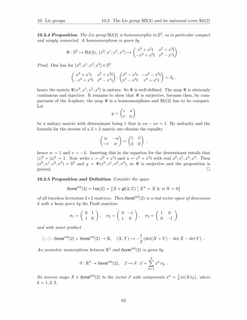
10. Lie groups 10.2. The Lie group SOp3q and its universal cover SUp2q
10.2.4 Proposition The Lie group SUp2q is homeomorphic to S3, so in particular compactand simply connected. A homeomorphism is given by
Ψ : S3 ÞÑ SUp2q, px0, x1, x2, x3q ÞÑ
ˆ
x0 ` x1i x2 ` x3i´x2 ` x3i x0 ´ x1i
˙
.
Proof. One has for px0, x1, x2, x3q P S3
ˆ
x0 ` x1i x2 ` x3i´x2 ` x3i x0 ´ x1i
˙
¨
ˆ
x0 ´ x1i ´x2 ´ x3ix2 ´ x3i x0 ` x1i
˙
“ I2 ,
hence the matrix Ψpx0, x1, x2, x3q is unitary. So Ψ is well-defined. The map Ψ is obviouslycontinuous and injective. It remains to show that Ψ is surjective, because then, by com-pactness of the 3-sphere, the map Ψ is a homeomorphism and SUp2q has to be compact.Let
g “
ˆ
z uv w
˙
be a unitary matrix with determinant being 1 that is zw ´ uv “ 1. By unitarity and theformula for the inverse of a 2ˆ 2 matrix one obtains the equality
ˆ
w ´u´v w
˙
“
ˆ
z vu w
˙
,
hence w “ z and v “ ´u. Inserting this in the equation for the determinant entails that|z|2 ` |u|2 “ 1. Now write z “ x0 ` x1i and u “ x2 ` x3i with real x0, x1, x2, x3. Thenpx0, x1, x2, x3q P S3 and g “ Ψpx0, x1, x2, x3q, so Ψ is surjective and the proposition isproved.
10.2.5 Proposition and Definition Consider the space
Hermtr0p2q “ i sup2q “
X P glp2,Cqˇ
ˇ X˚ “ X & trX “ 0(
of all traceless hermitian 2ˆ2 matrices. Then Hermtr0p2q is a real vector space of dimension3 with a basis given by the Pauli matrices
σ1 “
ˆ
0 11 0
˙
, σ2 “
ˆ
0 ´ii 0
˙
, σ3 “
ˆ
1 00 ´1
˙
and with inner product
x¨, ¨y : Hermtr0p2q ˆ Hermtr0p2q Ñ R, pX,Y q ÞÑ ´1
2pdetpX ` Y q ´ detX ´ detY q .
An isometric isomorphism between R3 and Hermtr0p2q is given by
~σ : R3 Ñ Hermtr0p2q, ~x ÞÑ ~σ ¨ ~x “3ÿ
k“1
xk σk .
Its inverse maps X P Hermtr0p2q to the vector ~x with components xk “ 12 trpXσkq, where
k “ 1, 2, 3.
62

10. Lie groups 10.2. The Lie group SOp3q and its universal cover SUp2q
Proof. Let X “
ˆ
a zw d
˙
P Hermtr0p2q. Then a, d P R and w “ z, since X is hermitian.
The assumption trX “ 0 implies d “ ´a. Hence X is of the formˆ
a b` c ib´ c i ´a
˙
“ aσ3 ` cσ1 ` bσ2
with a, c, d P R, and any such matrix is an element of Hermtr0p2q. Since the Pauli matricesare obviously linearly independent, they therefore form a basis of Hermtr0p2q.
Next compute for ~x “ px1, x2, x3q P R3
(10.2.5.1) det p~σ ¨ ~xq “ det
ˆ
x3 x2 ` x1 ix2 ´ x1 i ´x3
˙
“ ´px3q2 ´ px1q2 ´ px2q2 “ ´~x2 .
Hence the map Hermtr0p2q Ñ Rě0, X ÞÑa
´detpXq is a norm on Hermtr0p2q which has tofullfill the parallelogram identity since the euclidean norm ¨ does.
The norm on Hermtr0p2q is therefore induced by an inner product which can be recoveredby the polarization identity (8.1.10.1) that is by
xX,Y y “ ´1
2pdetpX ` Y q ´ detX ´ detY q for all X,Y P Hermtr0p2q .
Moreover, ~σ preserves norms by (10.2.5.1), hence is an isometry.
For the remaining part of the claim check first that pσkq2 “ I2 for k “ 1, 2, 3 and that
(10.2.5.2) σ1 σ2 “
ˆ
i 00 ´i
˙
“ iσ3, σ2 σ3 “
ˆ
0 ii 0
˙
“ iσ1, σ3 σ1 “
ˆ
0 1´1 0
˙
“ iσ2 .
Since the Pauli matrices are hermitian, forming the hermitian conjugate on both sides ofthese equations entails
(10.2.5.3) σ2 σ1 “ ´iσ3, σ3 σ2 “ ´iσ1, σ1 σ3 “ ´iσ2 .
Now compute for ~x P R3 and k “ 1, 2, 3
1
2tr pp~x ¨ ~σqσkq “
1
2tr`
xk pσkq2˘
“ xk .
The proposition is proved.
10.2.6 Lemma For i, j P t1, 2, 3u the Pauli matrices satisfy the following commutationrelations:
rσi, σjs “ 2i3ÿ
k“1
εijk σk ,
where for i, j, k P t1, 2, 3u the Levi-Civita symbol εijk is defined by
εijk “
$
’
&
’
%
1 if pi, j, kq is an even permutation of p1, 2, 3q,
´1 if pi, j, kq is an odd permutation of p1, 2, 3q, and
0 else.
63

10. Lie groups 10.2. The Lie group SOp3q and its universal cover SUp2q
10.2.7 Remark Recall that a permutation of p1, 2, 3q is even if and only if it is cyclic.
Proof. The commutation relations follow immediately from equations (10.2.5.2) and (10.2.5.3)in the proof of the preceding proposition.
10.2.8 Theorem The matrices
τ1 “1
iσ1 “
ˆ
0 ´i´i 0
˙
, τ2 “1
iσ2 “
ˆ
0 ´11 0
˙
, τ3 “1
iσ3 “
ˆ
´i 00 i
˙
form a basis of the Lie algebra sup2q and obey the commutation relations
(10.2.8.1) rτi, τjs “ 2τk for every cyclic permutation pi, j, kq of p1, 2, 3q .
Moreover, the linear map Φ : sup2q Ñ R3 uniquely defined by τk ÞÑ 2ek for k “ 1, 2, 3 isan isomorphism of Lie algebras, where R3 carries the Lie algebra structure given by thecross product ˆ. In particular, the Lie algebras sup2q and sop3q are isomorphic with anisomorphism given by
sup2q Ñ sop3q,3ÿ
k“1
xkτk “
ˆ
´x3i ´x2 ´ x1ix2 ´ x1i x3i
˙
ÞÑ 2
¨
˝
0 ´x3 x2
x3 0 ´x1
´x2 x1 0
˛
‚ .
Proof. Since multiplication by ´i is a real linear isomorphism from Hermtr0p2q to sup2qand since the Pauli matrices form a basis of Hermtr0p2q, the matrices τk, k “ 1, 2, 3, form abasis of sup2q. The commutation relations (10.2.8.1) are an immediate consequence of thepreceding lemma. The Lie bracket is preserved by Φ since
p2eiq ˆ p2ejq “ 2p2ekq for every cyclic permutation pi, j, kq of p1, 2, 3q .
The rest of the claim now follows by definition of Φ and Theorem 10.2.2.
10.2.9 Theorem For every g P SUp2q is the linear map
πg : R3 Ñ R3, ~x ÞÑ ~σ´1`
gp~σ ¨ ~xqg˚˘
an orthogonal transformation. Moreover, the map
π : SUp2q Ñ SOp3q, g ÞÑ πg
is a differentiable surjective group homomorphism with kernel t˘I2u – Z2. In particularπ is the universal covering map of SOp3q.
Proof. Since detpgAg˚q “ detA for all g P SUp2q and A P Hermtr0p2q and since ~σ is anisometric isomorphism from pR3, ¨ q to pHermtr0p2q,´1
2 detq, the transformations πg areorthogonal.
64

10. Lie groups 10.3. The Lorentz group SOp1, 3q and its universal cover SLp2,Cq
10.3. The Lorentz group SOp1, 3q and its universal cover SLp2,Cq
10.3.1 The Lorentz group Op1, 3q consists of all g P GLp4,Rq such that
xgx, gyyM “ xx, yyM for all x, y P R4 ,
where xx, yyM “ x0y0 ´ř3k“1 x
kyk denotes the Minowski product of two elements x “px0, x1, x2, x3q P R4 and y “ py0, y1, y2, y3q P R4 . Recall that R4 together with theMinkowski product is denoted R1,3 and called the Minkowski space of dimension 4.
Let us show that the Lorentz group SOp1, 3q is a Lie group.
10.3.2 The special linear group SLp2,Cq consists of all g P GLp2,Cq such that det g “ 1.It is a complex Lie group by the following argument. Observe that the determinant det :GLp2,Cq Ñ C is a complex differentiable group homomorphism. Its (complex) tangentmap at the identity is given by
T1 det : glp2,Cq Ñ C, A ÞÑB
Bz
ˇ
ˇ
ˇ
ˇ
z“0
det exppzAq “B
Bz
ˇ
ˇ
ˇ
ˇ
z“0
ez trpAq “ trA .
This entails that T1 det pzI2q “ 2z for each z P C hence det is a holomorphic submersionand SLp2,Cq “ det´1p1q a complex Lie group.
10.3.3 Proposition The Lie group SLp2,Cq is simply-connected.
Proof. We first show that SLp2q is path-connected. So let g P SLp2Cq. Then transform ginto Jordan normal form that is choose S P GLp2,Cq such that
SgS´1 “
ˆ
a1 e0 a2
˙
,
where a1, a2 P C with a1a2 “ 1 and e P t0, 1u. Then choose a path γ1 : r0, 1s Ñ Cˆ “ Czt0usuch that γ1p0q “ 1 and γ1p1q “ a1. Let γ2 : r0, 1s Ñ Cˆ be the path which maps t to
γ2ptq “`
γ1ptq˘´1
. Now put
hptq “ S´1
ˆ
γ1ptq te0 γ2ptqq
˙
.
Then h : r0, 1s Ñ SLp2,Cq is a continuous path connecting hp0q “ I2 with hp1q “ g. SoSLp2,Cq is path-connected.
Next we prove that SLp2,Cq is simply-connected. To this end recall that the subgroupSUp2q Ă SLp2,Cq is simply-connected. So to verify that π1
`
SLp2,Cq˘
is trivial it suffices toconstruct a (strong) deformation retraction from SLp2,Cq onto SUp2q that is a contimnuousmap r : SLp2,Cq ˆ r0, 1s Ñ SLp2,Cq such that
r0 “ id, r1
`
SLp2,Cq˘
Ă SUp2q, and rt|SUp2q “ idSUp2q for all t P r0, 1s .
Here, as usual, rt stands for the map SLp2,Cq Ñ SLp2,Cq, g ÞÑ rpg, tq.
65
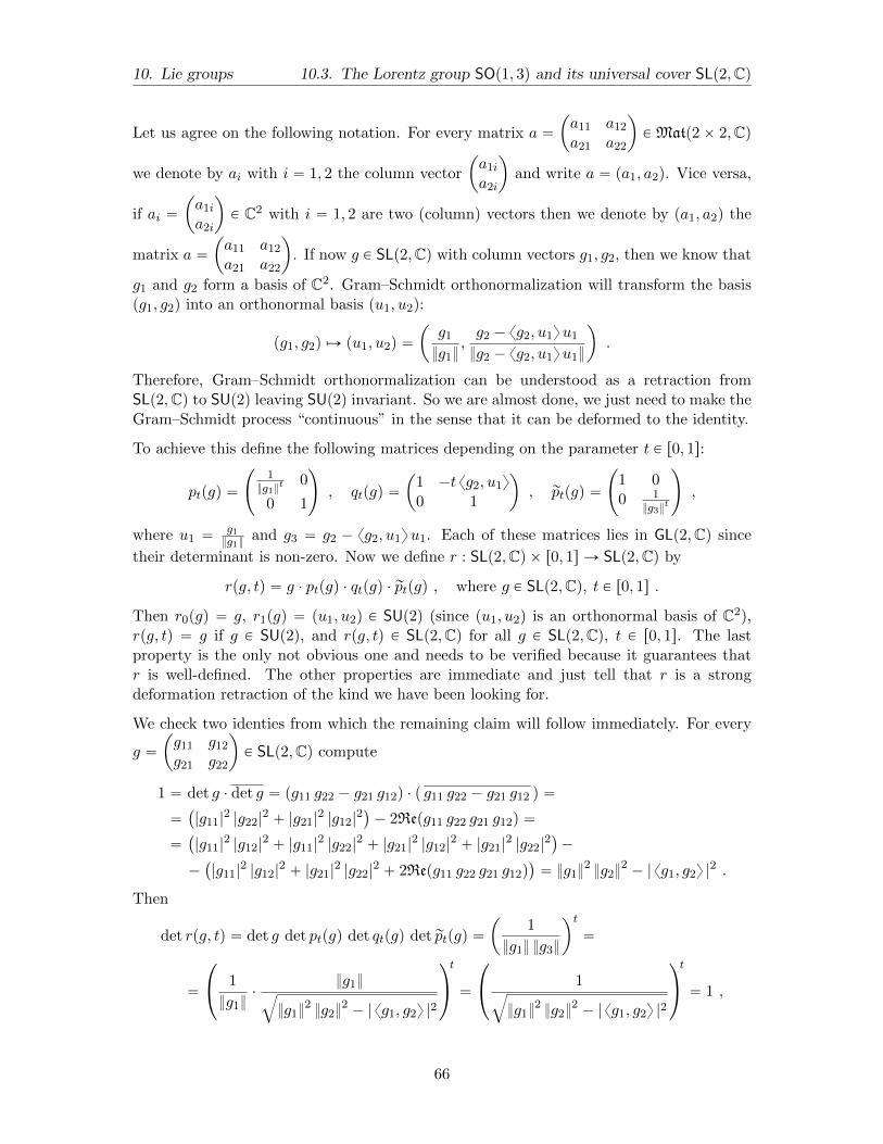
10. Lie groups 10.3. The Lorentz group SOp1, 3q and its universal cover SLp2,Cq
Let us agree on the following notation. For every matrix a “
ˆ
a11 a12
a21 a22
˙
PMatp2ˆ 2,Cq
we denote by ai with i “ 1, 2 the column vector
ˆ
a1i
a2i
˙
and write a “ pa1, a2q. Vice versa,
if ai “
ˆ
a1i
a2i
˙
P C2 with i “ 1, 2 are two (column) vectors then we denote by pa1, a2q the
matrix a “
ˆ
a11 a12
a21 a22
˙
. If now g P SLp2,Cq with column vectors g1, g2, then we know that
g1 and g2 form a basis of C2. Gram–Schmidt orthonormalization will transform the basispg1, g2q into an orthonormal basis pu1, u2q:
pg1, g2q ÞÑ pu1, u2q “
ˆ
g1
g1,g2 ´ xg2, u1yu1
g2 ´ xg2, u1yu1
˙
.
Therefore, Gram–Schmidt orthonormalization can be understood as a retraction fromSLp2,Cq to SUp2q leaving SUp2q invariant. So we are almost done, we just need to make theGram–Schmidt process “continuous” in the sense that it can be deformed to the identity.
To achieve this define the following matrices depending on the parameter t P r0, 1s:
ptpgq “
˜
1g1
t 0
0 1
¸
, qtpgq “
ˆ
1 ´t xg2, u1y
0 1
˙
, rptpgq “
˜
1 00 1
g3t
¸
,
where u1 “g1g1
and g3 “ g2 ´ xg2, u1yu1. Each of these matrices lies in GLp2,Cq since
their determinant is non-zero. Now we define r : SLp2,Cq ˆ r0, 1s Ñ SLp2,Cq by
rpg, tq “ g ¨ ptpgq ¨ qtpgq ¨ rptpgq , where g P SLp2,Cq, t P r0, 1s .
Then r0pgq “ g, r1pgq “ pu1, u2q P SUp2q (since pu1, u2q is an orthonormal basis of C2),rpg, tq “ g if g P SUp2q, and rpg, tq P SLp2,Cq for all g P SLp2,Cq, t P r0, 1s. The lastproperty is the only not obvious one and needs to be verified because it guarantees thatr is well-defined. The other properties are immediate and just tell that r is a strongdeformation retraction of the kind we have been looking for.
We check two identies from which the remaining claim will follow immediately. For every
g “
ˆ
g11 g12
g21 g22
˙
P SLp2,Cq compute
1 “ det g ¨ det g “ pg11 g22 ´ g21 g12q ¨ p g11 g22 ´ g21 g12 q “
“`
|g11|2 |g22|
2 ` |g21|2 |g12|
2˘
´ 2Repg11 g22 g21 g12q “
“`
|g11|2 |g12|
2 ` |g11|2 |g22|
2 ` |g21|2 |g12|
2 ` |g21|2 |g22|
2˘
´
´`
|g11|2 |g12|
2 ` |g21|2 |g22|
2 ` 2Repg11 g22 g21 g12q˘
“ g12g2
2´ | xg1, g2y |
2 .
Then
det rpg, tq “ det g det ptpgq det qtpgq det rptpgq “
ˆ
1
g1 g3
˙t
“
“
¨
˝
1
g1¨
g1b
g12g2
2´ | xg1, g2y |
2
˛
‚
t
“
¨
˝
1b
g12g2
2´ | xg1, g2y |
2
˛
‚
t
“ 1 ,
66

10. Lie groups 10.3. The Lorentz group SOp1, 3q and its universal cover SLp2,Cq
which means that rpg, tq is in fact an element of SLp2,Cq for all g P SLp2,Cq and t P r0, 1s.This finishes the proof.
10.3.4 Proposition and Definition Consider the space
Hermp2q “
X P glp2,Cqˇ
ˇ X˚ “ X(
of all hermitian 2ˆ 2 matrices. Then Hermp2q is a real vector space of dimension 4 with abasis given by the identity matrix plus the Pauli matrices that is by
σ0 “
ˆ
1 00 1
˙
, σ1 “
ˆ
0 11 0
˙
, σ2 “
ˆ
0 ´ii 0
˙
, σ3 “
ˆ
1 00 ´1
˙
and with inner product
x¨, ¨y : Hermp2q ˆ Hermp2q Ñ R, pX,Y q ÞÑ ´1
2pdetpX ` Y q ´ detX ´ detY q .
An isometric isomorphism between R4 and Hermp2q is given by
σ : R4 Ñ Hermp2q, x ÞÑ σ ¨ x “3ÿ
k“0
xk σk .
Its inverse maps X P Hermp2q to the vector x with components xk “ 12 trpXσkq, where
k “ 0, 1, 2, 3.
10.3.5 Theorem For every g P SLp2,Cq is the linear map
πg : R4 Ñ R4, x ÞÑ σ´1`
gpσ ¨ xqg˚˘
a proper orthochronous Lorentz transformation. Moreover, the map
π : SUp2q Ñ SOÒp1, 3q, g ÞÑ πg
is a differentiable surjective group homomorphism with kernel t˘I2u – Z2. In particularπ is the universal covering map of SOÒp1, 3q.
Proof.
67
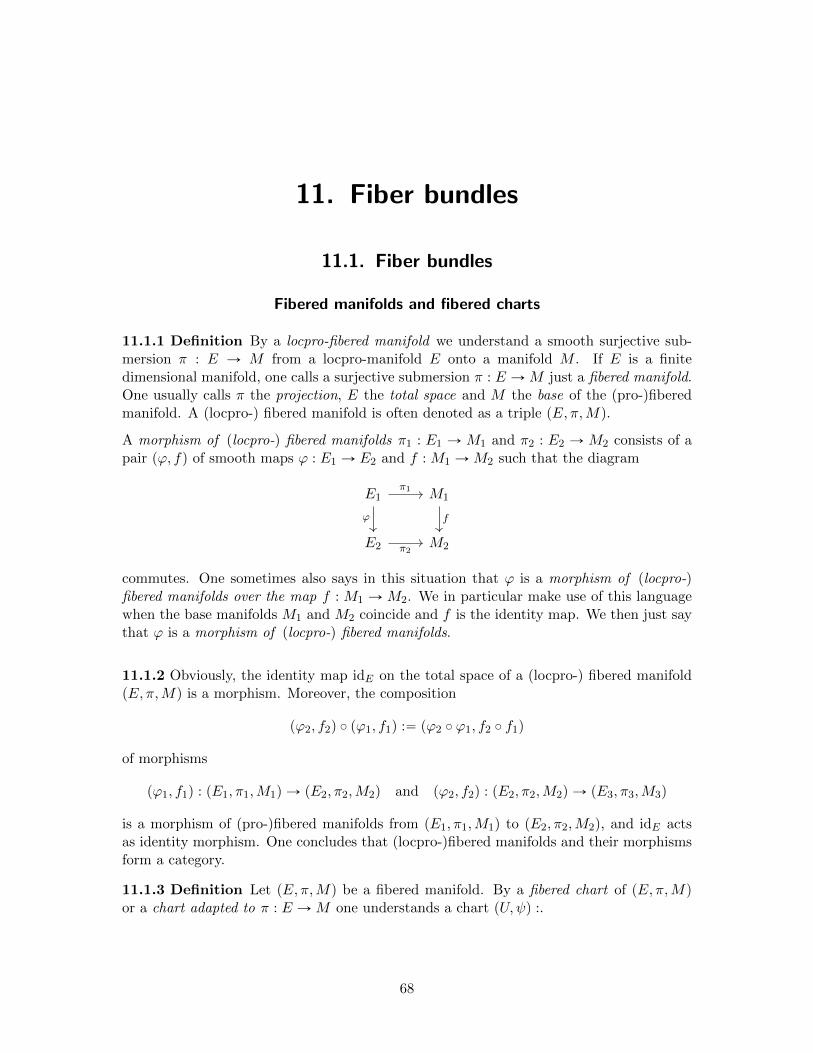
11. Fiber bundles
11.1. Fiber bundles
Fibered manifolds and fibered charts
11.1.1 Definition By a locpro-fibered manifold we understand a smooth surjective sub-mersion π : E Ñ M from a locpro-manifold E onto a manifold M . If E is a finitedimensional manifold, one calls a surjective submersion π : E ÑM just a fibered manifold.One usually calls π the projection, E the total space and M the base of the (pro-)fiberedmanifold. A (locpro-) fibered manifold is often denoted as a triple pE, π,Mq.
A morphism of (locpro-) fibered manifolds π1 : E1 Ñ M1 and π2 : E2 Ñ M2 consists of apair pϕ, fq of smooth maps ϕ : E1 Ñ E2 and f : M1 ÑM2 such that the diagram
E1 M1
E2 M2
π1
ϕ f
π2
commutes. One sometimes also says in this situation that ϕ is a morphism of (locpro-)fibered manifolds over the map f : M1 Ñ M2. We in particular make use of this languagewhen the base manifolds M1 and M2 coincide and f is the identity map. We then just saythat ϕ is a morphism of (locpro-) fibered manifolds.
11.1.2 Obviously, the identity map idE on the total space of a (locpro-) fibered manifoldpE, π,Mq is a morphism. Moreover, the composition
pϕ2, f2q ˝ pϕ1, f1q :“ pϕ2 ˝ ϕ1, f2 ˝ f1q
of morphisms
pϕ1, f1q : pE1, π1,M1q Ñ pE2, π2,M2q and pϕ2, f2q : pE2, π2,M2q Ñ pE3, π3,M3q
is a morphism of (pro-)fibered manifolds from pE1, π1,M1q to pE2, π2,M2q, and idE actsas identity morphism. One concludes that (locpro-)fibered manifolds and their morphismsform a category.
11.1.3 Definition Let pE, π,Mq be a fibered manifold. By a fibered chart of pE, π,Mqor a chart adapted to π : E ÑM one understands a chart pU,ψq :.
68

11. Fiber bundles 11.1. Fiber bundles
11.1.4 Proposition Given a locpro-fibered manifold pE, π,Mq, the fiber Fp :“ π´1ppqover an element p PM is a locpro-manifold.
Proof. In the case where E is finite dimensional the claim is an immediate consequence ofthe submersion theorem So assume that E is infinite dimensional. Since the claim is local,we can assume that there exists a smooth projective representation pEi, ηij , ηiqi,jPN, iďj ofE. Since M is finite dimensional and using again that the claim is local we can assumethat the the smooth map π : E Ñ M factors in a neighborhood of Fp through somesmooth map πi : Ei Ñ M that means that π “ πi ˝ ηi. Since π is a smooth surjectivesubmersion, πi is so, too. Therefore, Fi :“ π´1
i ppq is a submanifold of Ei by the submersiontheorem. Now put πj :“ πi ˝ ηij for all j ą i. As a composition of surjective submersionseach such πj is a surjective submersion as well. Hence for every j ą i the preimageFj :“ π´1
j ppq “ η´1ij pFiq is a submanifold of Ej . Since π “ πi ˝ ηi “ πi ˝ ηij ˝ ηj “ πj ˝ ηj ,
the fiber Fp coincides with η´1j pFjq for each j ě i. Hence we obtain a smooth projective
representation pFj , ϕjk, ϕjqj,kPN jďk of Fp, when defining ϕjk as the restriction ηjk|Fk andϕj as the restriction ηj |Fp . So Fp is a pro-manifold and the claim is proved.
11.1.5 Proposition A locpro-fibered manifold has local smooth sections that is for everylocpro-fibered manifold pE, π,Mq and every point p P M there exists as smooth map s :U Ñ E defined on an open neighborhood U of p in M such that π ˝ s “ idU .
69

12. Jets
12.1. A combinatorial interlude
Multiindices
12.1.1 Assume that I is a non-empty set which we call index set. By a multiindex over I
we then understand an element α P NpIq that is a family α “ pαiqiPI of natural numberssuch that only finitely many αi are non-zero. The order of such a multiindex is definedby |α| :“
ř
iPI αi. For k P N and k1 P N and k2 P N Y t8u with k1 ď k2 we denote by
NpIqk the set of all multiindices over I of order k and by NpIqk1,k2 the set of all multiindices oforder less or equal k2 which have order greater or equal k1. For reasons of clarity, whichwill be become obvious below, we sometimes also refer to an element of NpIq as a Greekmultiindex.
12.1.2 Example In most cases the index set I will be of the form I “ t1, . . . , du or ofthe form I “ t0, . . . , d ´ 1u for some positive integer d. One then has NpIq “ NI “ Ndand multiindices are given by d-tuples of the form α “ pα1, . . . , αdq or β “ pβ0, . . . , βd´1q,respectively.
12.1.3 The space of multiindices NpIq carries the structure of a module over the semiring Nin the sense of Johnson & Manes (1970) that is NpIq together with componentwise additionis an abelian monoid, componentwise multiplication with scalars is associative, 0 acts aszero map, 1 acts as identity, and the distributivity laws hold true. Moreover, NpIq is freeover the family of multiindices p1iqiPI defined by
1ipjq :“
#
1 for j “ i,
0 else.
12.1.4 By a Roman multiindex of a given order k P Ną0 over some index set I we under-stand an element I of the cartesian product Ik. For k “ 0 we define I0 as the set tOu,where O is a fixed set not appearing as an element of I. We call O the Roman multiindexof order 0 over I. We sometimes write |I| for the order of a Roman multiindex. Note thatwe denote elements of Ik by capital Roman letters I, J, . . . and their components by theirrespective small Roman letters il, jl, and so on.
For k ě 1 the symmetric group Sk acts in a canoncial way on Ik. We denote the orbitspace of this action by Ik and the orbit through a Roman multiindex I P Ik by I. In otherwords I is the equivalence class of all Roman multiindices obtained from I by permutationof its components. For k “ 0 we identify I0 with I0 and O with O.
70

12. Jets 12.1. A combinatorial interlude
For Roman multiindices I “ pi1, . . . , ikq P Ik and J “ pj1, . . . , jlq P Il of positive order wedenote by I`J the multiindex pi1, . . . , ik, j1, . . . , jlq P I
k`l. Obviously, the equivalence classI ` J depends only on the equivalence classes I and J , hence the operation ` descends toa map
` : IkSk ˆ IlSl Ñ Ik`lSk`l .
It is straightforward to see that this operation is associative and commutative. Next defineI`O “ O`I “ I and I`O “ O`I “ I for all Roman multiindices I and set I‚ :“ I‚ „,where I‚ :“
Ů
kPN Ik and„ is the equivalence relation which defines two Roman multiindices
I P Ik and J P Il as equivalent if k “ l and I “ J . Then I‚ “Ů
kPN Ik. Moreover, I‚
together with ` as binary operation and O as zero element becomes an abelian monoid.
Note that every i P I can be regarded as a Roman multiindex of order 1 and that i “ i, sowe have the sums I ` i “ pi1, . . . , ik, iq and I ` i “ pi1, . . . , ik, iq. Sometimes we also writeI, i respectively I, i for these sums.
12.1.5 Lemma Assume that I is totally ordered by some order relation ď. Then everyelement of Ik of order k P Ną0 has a unique representative I “ pi1, . . . , ikq P Ik suchthat i1 ď i2 ď . . . ď ik. We call such a representative an increasing representative or ofincreasing form.
Proof. One proves the claim by induction on the order k. For k “ 1 the claim is obvious.Assume that it holds for some k and let J be a Roman multiindex of order k ` 1. Letjm be the maximum of the components j1, . . . , jk`1, and let σ P Sk`1 be the permutationswitching m and k ` 1 and acting by identity on the rest. By hypothesis there exists apermutation τ P Sk such that jστp1q ď . . . ď jστpkq. Put τpk ` 1q “ k ` 1. Then τ P Sk`1
and I “ pjστp1q, . . . , jστpk`1qq is a representative of J with the desired properties. Thisfinishes the inductive step and the claim is proved.
12.1.6 Proposition Let I be an index set with a total order ď on it and κ : NpIq Ñ I‚ themap which maps the zero map 0I : IÑ N to O and a Greek multiindex α of positive orderto the Roman multiindex
`
i1, . . . , i1looomooon
αi1 times
, i2, . . . , i2looomooon
αi2 times
, . . . , il, . . . , illooomooon
αil times
˘
,
where i1 ă . . . ă il are the (pairwise distinct and ordered) elements i P I with non-vanishingcomponent αi. Then the induced map κ : NpIq Ñ I‚, α ÞÑ κpαq is an isomorphism of
monoids and maps the space NpIqk of Greek multiindices of order k onto Ik. Moreover, if I
is finite, then NpIqk and Ik are finite as well and both have cardinality given by
|NIk| “ |I
k| “1
k!
k´1ź
l“0
`
|I| ` l˘
.
Proof. First we need to show that κ is a bijection. To this end let us make our notationsomewhat more precise and choose for each α P NpIqzt0Iu the elements iα1 , . . . , i
αlαP I so
71
12. Jets 12.1. A combinatorial interlude
that iα1 ă . . . ă iαlα , αiαj ą 0 for j “ 1, . . . , lα and αi “ 0 for all i P Iztiα1 , . . . , iαlαu. Then
κpαq “`
iα1 , . . . , iα1
loooomoooon
αiα1times
, iα2 , . . . , iα2
loooomoooon
αiα2times
, . . . , iαlα , . . . , iαlα
loooomoooon
αiαlα
times
˘
.
By construction, κpαq is of increasing form. For each element I P I‚ let I be the represen-tative of increasing form. Define λpIq P NpIq as follows. If I “ O, put λpIq “ 0I. If I ‰ O,let iI1 ă . . . ă iIlI be the elements of I which appear in I. Then, for each j “ 1, . . . , lI define
αIiIj
to be the number of times the index iIj appears in I. For i P I not appearing among
the iIj put αIi “ 0. Then define
λpIq “ αI “`
αIi˘
iPI.
So we obtain a map λ : I‚ Ñ NpIq. For given I ‰ O one has by definition lαI “ lIand iα
I
1 “ iI1, . . . , iαI
l “ iIl where l “ lαI “ lI . Moreover, the index i “ iαI
j , j “ 1, . . . , l
appears in κ`
λpIq˘
exactly αIi times which coincides with the number i appears in I. Henceκ`
λpIq˘
“ I. Now assume α P NIzt0Iu to be given and let I “ κpαq. Then lI “ lα andiI1 “ iα1 , . . . , i
Il “ iαl for l “ lI “ lα. Now observe that for each of the indices i “ iIj ,
j “ 1, . . . , l the i-th component of λ`
κpαq˘
coincides with αi. Hence λ`
κpαq˘
“ α, whichfinishes the proof that κ is a bijection with inverse λ.
By construction of κ one has |κpαq| “ |α| for all Greek multiindices α which entails that
for every k P N the bijection κ maps NpIqk onto Ik.
Also by construction it is clear that κpα ` βq “ κpαq ` κpβq for all α, β P NpIq and thatκp0Iq “ O. Hence κ is a morphism of monoids.
Now we will prove the formula for the cardinality of NIk by double induction on k and the
cardinality of the index set I. Obviously |NI0| “ 1, so the claim holds for k “ 0 and all
finite index sets. Assume that it holds for some natural k and all finite index sets. Now letI be an index set of cardinality 1. Then |NI
k`1| “ 1 since there is only one natural numberwith absolute value k ` 1. Next assume that the claim holds for k ` 1 and all index setsof cardinality less than d. Let I be an index set of cardinality d. Order the elements of Iin some way so that I “ ti1, . . . , idu and i1 ă . . . ă id. The set NI
k`1 is then the disjoint
union of the set of all α P NIk`1 such that αid “ 0 and the set of all α P NI
k`1 such thatαid ě 1. The first of these sets has cardinality
|Nti1,...,id´1u
k`1 | “1
k ` 1!
kź
l“0
`
d´ 1` l˘
,
the second has cardinality
|NIk| “
1
k!
k´1ź
l“0
`
d` l˘
since the map
α P NIk`1
ˇ
ˇ αid ě 1(
Ñ NIk : α ÞÑ pαi1 , . . . , αid´1
, αid ´ 1q P NIk
72

12. Jets 12.1. A combinatorial interlude
is a bijection. Hence
|NIk`1| “
1
k ` 1!
kź
l“0
`
d´ 1` l˘
`1
k!
k´1ź
l“0
`
d` l˘
“
“1
k ` 1!pd´ 1` k ` 1q
k´1ź
l“0
`
d` l˘
“1
pk ` 1q!
kź
l“0
`
d` l˘
and the induction step is finished. The claim is proved.
12.1.7 By a block of a Roman multiindex I of positive order we mean a Roman multiindexof the form
IB “ pib1 , . . . , ib|B|q ,
where B is a subset of t1, . . . ku and the b1, . . . , b|B| P t1, . . . , ku are the elements of Bin increasing order. One can now decompose a multiindex I into blocks as follows. LettB1, . . . , Bru be a partition of t1, . . . , ku which we assume to be lexicographically orderedthat means that b11 ă b21 ă . . . ă br1, where Bj “ tbj1, . . . , bj|Bj |u and bjm ă bjn forj “ 1, . . . , r and 1 ď m ă n ď |Bj |. To express that tB1, . . . , Bru is a lexicographicallyordered partition of t1, . . . , ku by r non-empty sets we write
B1 \ . . .\Br “ t1, . . . , ku & H ă B1 ă . . . ă Br .
Now put Ij :“ IBj for j “ 1, . . . , r. Then the Roman multiindices I and I1 ` . . . ` Ir areequivalent which can be interpreted as I being decomposed into the r blocks I1, . . . , Ir.More precisely, we call the r-tupel of pairs
`
pI1, B1q, . . . , pIr, Brq˘
a a decomposition of Iinto r blocks and denote the space of such decompositions by BlockrpIq. Note that thecardinality of BlockrpIq coincides with the Sterling number of the second kind
kr
(
whichgives the number of ways the set t1, . . . , ku can be partitioned into r subsets.
Multipowers and multiderivatives
12.1.8 Let M be a manifold and x “ px1, . . . , xdq : U Ñ Rd a local coordinate system. LetI P t1, . . . , duk be a Roman multiindex of positive order k. Then the product
(12.1.8.1) xI :“ xi1 ¨ . . . ¨ xik
and, for every f P C8pUq, the higher derivative
(12.1.8.2)B|I|f
BxI:“
Bkf
Bxi1 ¨ . . . ¨ Bxik
are both invariant under permutations of the components of I, hence depend only on the
equivalence class I. We therefore sometimes write xI for xI and B|I|f
BxIfor B|I|f
BxI. In order 0
one puts xO :“ xO :“ 1 and B|O|f
BxO:“ B|O|f
BxO:“ f . For a multiindex α P Nd one defines as
usual
xα :“ px1qα1 ¨ . . . ¨ pxdqαd
73

12. Jets 12.1. A combinatorial interlude
and
B|α|f
Bxα:“
B|α|f
pBx1qα1 ¨ . . . ¨ pBxdqαd:“
ˆ
B
Bx1
˙α1
¨ . . . ¨
ˆ
B
Bxd
˙αd
f .
If now α and I are related by I “ κpαq, then xI “ xα and B|I|f
BxI“B|α|fBxα by definition of κ
and invariance of the product and the higher derivative under permutations of componentsof the multiindex.
12.1.9 Remark Occasionally we need multipowers and multiderivatives over more generalindex sets. So let I be an arbitrary but still finite index set. Assume that the componentsof a coordinate system x : U Ñ RI are labelled xi where i runs through the elements of I.For I P Ik equations (12.1.8.1) and (12.1.8.2) then can be used again to define multipowers
xI and multiderivatives B|I|fBxI
. Note that both objects are invariant under permutations of
components of I, too, so the corresponding expressions where I is replaced by I are alsowell-defined. Now let α “ pαiqiPI P NI be a Greek multiindex and f P C8pUq. One thendefines
xα :“ź
iPI
pxiqαi
andB|α|f
Bxα:“
ź
iPI
ˆ
B
Bxi
˙αi
f .
One finally checks that when κpαq “ I the equalities xα “ xI and B|α|fBxα “
B|I|f
BxIstill hold
true in this more general situation.
The formula of Faa-di-Bruno
12.1.10 Theorem (Combinatorial form of the formula of Faa-di-Bruno) Let Iand J be finite index sets. Assume that M and N are smooth manifolds and that we aregiven smooth charts x : U ãÑ RI and y : V ãÑ RJ over open domains U ĂM and V Ă N .Asuume further that ϕ : U Ñ V is a smooth map. Denote by ϕj : U Ñ R, j P J itscomponents that means that ϕ “ pϕjqjPJ . Finally let I P Ik be a Roman multiindex ofpositive order k. Then for every f P C8pV q the following equality holds true:(12.1.10.1)
B|I|pf ˝ ϕq
BxI“
kÿ
r“1
ÿ
JPJ rJ“pj1,...,jrq
ÿ
B1\...\Br“t1,...,kuHăB1ă...ăBr
˜
B|J |f
ByJ˝ϕ
¸
¨B|IB1
|ϕj1
BxIB1¨ . . . ¨
B|IBr |ϕjr
BxIBr.
Proof. We prove the claim by induction on the length of the multiindex I. Assume to begiven a Roman multiindex I P Ik of length k “ |I| “ 1. Then there exists a unique i P Isuch that I “ piq. By the chain rule one computes
B|I|pf ˝ ϕq
BxI“Bpf ˝ ϕq
Bxi“
ÿ
jPJ
ˆ
Bf
Byj˝ ϕ
˙
¨Bϕj
Bxi“
ÿ
JPJ 1
J“pj1q
ÿ
B1“t1u
˜
B|J |f
ByJ˝ϕ
¸
¨B|IB1
|ϕj1
BxIB1,
74

12. Jets 12.2. Jet bundles
hence the claim holds true for k “ 1.
Now assume that for some k ě 1 the claim holds for all Roman multiindices of order ď kover I. Assume that I “ pi1, . . . , ik`1q is a Roman multiindex of order k` 1 over I. ThenI “ I 1` ik`1, where I 1 “ pi1, . . . , ikq is a Roman multiindex of order k. Using the inductionhypothesis for I 1, the product and the chain rule one obtains
B|I|pf ˝ ϕq
BxI“
B
Bxik`1
B|I1|
BxI 1f ˝ ϕ “
“B
Bxik`1
kÿ
r“1
ÿ
JPJ rJ“pj1,...,jrq
ÿ
B1\...\Br“t1,...,kuHăB1ă...ăBr
˜
B|J |f
ByJ˝ϕ
¸
¨B|IB1
|ϕj1
BxIB1¨ . . . ¨
B|IBr |ϕjr
BxIBr“
“
kÿ
r“1
ÿ
JPJ rJ“pj1,...,jrq
ÿ
jr`1PJ
ÿ
B1\...\Br“t1,...,kuHăB1ă...ăBr
˜
B|J |`1f
ByJjr`1˝ϕ
¸
¨B|IB1
|ϕj1
BxIB1¨ . . . ¨
B|IBr |ϕjr
BxIBr
Bϕjr`1
Bxik`1`
`
kÿ
r“1
rÿ
l“1
ÿ
JPJ rJ“pj1,...,jrq
ÿ
B1\...\Br“t1,...,kuHăB1ă...ăBr
˜
B|J |f
ByJ˝ϕ
¸
¨B|IB1
|ϕj1
BxIB1¨ . . . ¨
B|IBl |`1ϕjl
BxIBl ik`1¨ . . . ¨
B|IBr |ϕjr
BxIBr“
“
k`1ÿ
r“2
ÿ
JPJ rJ“pj1,...,jrq
ÿ
B1\...\Br“t1,...,k`1uHăB1ă...ăBr“tk`1u
˜
B|J |f
ByJ˝ϕ
¸
¨B|IB1
|ϕj1
BxIB1¨ . . . ¨
B|IBr |ϕjr
BxIBr`
`
kÿ
r“1
ÿ
JPJ rJ“pj1,...,jrq
ÿ
B1\...\Br“t1,...,k`1uHăB1ă...ăBr‰tk`1u
˜
B|J |f
ByJ˝ϕ
¸
¨B|IB1
|ϕj1
BxIB1¨ . . . ¨
B|IBr |ϕjr
BxIBr“
“
k`1ÿ
r“1
ÿ
JPJ rJ“pj1,...,jrq
ÿ
B1\...\Br“t1,...,k`1uHăB1ă...ăBr
˜
B|J |f
ByJ˝ϕ
¸
¨B|IB1
|ϕj1
BxIB1¨ . . . ¨
B|IBr |ϕjr
BxIBr.
This concludes the induction step and the theorem is proved.
12.2. Jet bundles
12.2.1 Let us fix in this section a smooth finite dimensional fiber bundle πE : E Ñ M .Denote by F its typical fiber and put d “ dimM , n “ dimF . The dimension of thetotal space E then is given by dimE “ d ` n. Note that for each point p P M the fiberFp “ pπ
Eq´1ppq is diffeomorphic to F .
Recall that Γ8pπEq stands for the sheaf of smooth local sections of πE . Its space of sectionsover an open U ĂM consists of all smooth s : U Ñ E such that πE ˝s “ idU and is denotedby Γ8pU, πEq. When writing s P Γ8pπEq we mean that s is a smooth local section of Edefined over some open subset U “ dom s Ă M . If p P X is a point, then Γ8pp, πEqdenotes the space of local smooth sections about p that is the space of all smooth sectionss : U Ñ E defined on an open neighborhood U Ă X of p. We will write U˝p for the filter
75

12. Jets 12.2. Jet bundles
basis of all open neighborhoods of p and Γ8p pπEq for the stalk of Γ8pπEq at p which is
defined as the colimit
(12.2.1.1) Γ8p pπEq “ colim
UPU˝pΓ8pU, πEq “ Γ8pp, πEq „p .
Here we have made use of the fact that the colimit can be represented as the quotientof Γ8pp, πEq by the equivalence relation „p, where equivalence s1 „p s2 of two smoothsections s1 : U1 Ñ E and s2 : U2 Ñ E over open neighborhoods of p is defined by theexistance of an open neighborhood U Ă U1XU2 of p such that s1|U :“ s2|U . The equivalenceclass of a section s P Γ8pp, πEq is denoted rssp and is called the germ of s at p. So in otherwords, Γ8p pπ
Eq is the space of all germs of smooth sections at p. To distinguish „p fromthe later defined m-equivalence we call the relation „p germ equivalence at p.
12.2.2 Definition Let p P M be a point in the base manifold M and k P NY t8u. Twolocal smooth sections s1 : U1 Ñ E and s2 : U2 Ñ E defined over open neighborhoods of pare said to be k -equivalent at p if s1ppq “ s2ppq and if for every fibered chart px, uq : W Ñ
Rd ˆ Rn of πE with p P πpW q
(12.2.2.1)B|α|pub ˝ s1q
Bxαppq “
B|α|pub ˝ s2q
Bxαppq for b “ 1, . . . , n and all α P Nd0,k .
12.2.3 Proposition and Definition Let p P M be a point and k P N Y t8u. Then k-equivalence at p is an equivalence relation on Γ8pp, πEq. It will be denoted by the symbol„k,p. The k-equivalence class of a smooth section s : U Ñ E at p will be written jkppsq. Itis called the k-jet of s at p. The set of such k-jets at p coincides with the quotient spaceJkppπ
Eq “ Γ8pp, πEq „k,p. The union
JkpEq “ JkpπEq “ď
pPM
JkppπEq
will be called the space of k-jets of sections of the bundle πE : E Ñ M . Finally, thereis a projection πk “ πJ
kpEq : JkpπEq Ñ M which maps a jet jkppsq, s P Γ8pp, πEq to itsfootpoint p.
Proof. The relation of k-equivalence at p is obviously reflexive and symmetric by definition.It is also transitive by transitivity of equality. Hence k-equivalence at p is an equivalencerelation indeed. The claim is proved.
12.2.4 Lemma The following statements are equivalent for two sections s1, s2 P Γ8pp, πEqsuch that s1ppq “ s2ppq:
(1) The local sections s1 and s2 are k-equivalent at p.
(2) For every fibered chart px, uq : W Ñ Rd ˆ Rn of πE with p P πpW q
B|I|pub ˝ s1q
BxIppq “
B|I|pub ˝ s2q
BxIppq for b “ 1, . . . , n and all
I P t1, . . . , dul, 1 ď l ď k .
(12.2.4.1)
76
12. Jets 12.2. Jet bundles
(3) There exists a fibered chart px, uq : W Ñ Rd ˆ Rn of πE with p P πpW q such that(12.2.2.1) holds true.
(4) There exists a fibered chart px, uq : W Ñ Rd ˆ Rn of πE with p P πpW q such that(12.2.4.1) holds true.
Proof. The claim is an immediate consequence of the formula of Faa-di-Bruno.
12.2.5 Next we want to define a topology on the jet space JkpπEq so that πk : JkpπEq ÑMbecomes a (topological) fiber bundle.
77

Licensing
Creative Commons Attribution-NonCommercial-NoDerivatives4.0 International
===================================================
Creative Commons Corporation (“Creative Commons”) is not a law firm and does notprovide legal services or legal advice. Distribution of Creative Commons public licensesdoes not create a lawyer-client or other relationship. Creative Commons makes its licensesand related information available on an “as-is” basis. Creative Commons gives no war-ranties regarding its licenses, any material licensed under their terms and conditions, orany related information. Creative Commons disclaims all liability for damages resultingfrom their use to the fullest extent possible.
Using Creative Commons Public Licenses
Creative Commons public licenses provide a standard set of terms and conditions thatcreators and other rights holders may use to share original works of authorship and othermaterial subject to copyright and certain other rights specified in the public license below.The following considerations are for informational purposes only, are not exhaustive, anddo not form part of our licenses.
Considerations for licensors: Our public licenses are
intended for use by those authorized to give the public
permission to use material in ways otherwise restricted by
copyright and certain other rights. Our licenses are
irrevocable. Licensors should read and understand the terms
and conditions of the license they choose before applying it.
Licensors should also secure all rights necessary before
applying our licenses so that the public can reuse the
material as expected. Licensors should clearly mark any
material not subject to the license. This includes other CC-
licensed material, or material used under an exception or
limitation to copyright. More considerations for licensors:
wiki.creativecommons.org/Considerations_for_licensors
Considerations for the public: By using one of our public
licenses, a licensor grants the public permission to use the
licensed material under specified terms and conditions. If
78

Licensing CC BY-NC-ND 4.0
the licensor’s permission is not necessary for any reason--for
example, because of any applicable exception or limitation to
copyright--then that use is not regulated by the license. Our
licenses grant only permissions under copyright and certain
other rights that a licensor has authority to grant. Use of
the licensed material may still be restricted for other
reasons, including because others have copyright or other
rights in the material. A licensor may make special requests,
such as asking that all changes be marked or described.
Although not required by our licenses, you are encouraged to
respect those requests where reasonable. More_considerations
for the public:
wiki.creativecommons.org/Considerations_for_licensees
===================================================
Creative Commons Attribution-NonCommercial-NoDerivatives 4.0 International Public Li-cense
By exercising the Licensed Rights (defined below), You accept and agree to be bound by theterms and conditions of this Creative Commons Attribution-NonCommercial-NoDerivatives4.0 International Public License (“Public License”). To the extent this Public License maybe interpreted as a contract, You are granted the Licensed Rights in consideration of Youracceptance of these terms and conditions, and the Licensor grants You such rights in con-sideration of benefits the Licensor receives from making the Licensed Material availableunder these terms and conditions.
Section 1 – Definitions.
a. Adapted Material means material subject to Copyright and Similar Rights that isderived from or based upon the Licensed Material and in which the Licensed Materialis translated, altered, arranged, transformed, or otherwise modified in a mannerrequiring permission under the Copyright and Similar Rights held by the Licensor.For purposes of this Public License, where the Licensed Material is a musical work,performance, or sound recording, Adapted Material is always produced where theLicensed Material is synched in timed relation with a moving image.
b. Copyright and Similar Rights means copyright and/or similar rights closely relatedto copyright including, without limitation, performance, broadcast, sound record-ing, and Sui Generis Database Rights, without regard to how the rights are labeledor categorized. For purposes of this Public License, the rights specified in Section2(b)(1)-(2) are not Copyright and Similar Rights.
c. Effective Technological Measures means those measures that, in the absence of properauthority, may not be circumvented under laws fulfilling obligations under Article11 of the WIPO Copyright Treaty adopted on December 20, 1996, and/or similarinternational agreements.
79

Licensing CC BY-NC-ND 4.0
d. Exceptions and Limitations means fair use, fair dealing, and/or any other exceptionor limitation to Copyright and Similar Rights that applies to Your use of the LicensedMaterial.
e. Licensed Material means the artistic or literary work, database, or other material towhich the Licensor applied this Public License.
f. Licensed Rights means the rights granted to You subject to the terms and conditionsof this Public License, which are limited to all Copyright and Similar Rights thatapply to Your use of the Licensed Material and that the Licensor has authority tolicense.
g. Licensor means the individual(s) or entity(ies) granting rights under this Public Li-cense.
h. NonCommercial means not primarily intended for or directed towards commercialadvantage or monetary compensation. For purposes of this Public License, the ex-change of the Licensed Material for other material subject to Copyright and SimilarRights by digital file-sharing or similar means is NonCommercial provided there isno payment of monetary compensation in connection with the exchange.
i. Share means to provide material to the public by any means or process that requirespermission under the Licensed Rights, such as reproduction, public display, publicperformance, distribution, dissemination, communication, or importation, and tomake material available to the public including in ways that members of the publicmay access the material from a place and at a time individually chosen by them.
j. Sui Generis Database Rights means rights other than copyright resulting from Di-rective 96/9/EC of the European Parliament and of the Council of 11 March 1996on the legal protection of databases, as amended and/or succeeded, as well as otheressentially equivalent rights anywhere in the world.
k. You means the individual or entity exercising the Licensed Rights under this PublicLicense. Your has a corresponding meaning.
Section 2 – Scope.
a. License grant.
1. Subject to the terms and conditions of this Public License, the Licensor herebygrants You a worldwide, royalty-free, non-sublicensable, non-exclusive, irrevo-cable license to exercise the Licensed Rights in the Licensed Material to:
a. reproduce and Share the Licensed Material, in whole or
in part, for NonCommercial purposes only; and
b. produce and reproduce, but not Share, Adapted Material
for NonCommercial purposes only.
80

Licensing CC BY-NC-ND 4.0
2. Exceptions and Limitations. For the avoidance of doubt, where Exceptions andLimitations apply to Your use, this Public License does not apply, and You donot need to comply with its terms and conditions.
3. Term. The term of this Public License is specified in Section 6(a).
4. Media and formats; technical modifications allowed. The Licensor authorizesYou to exercise the Licensed Rights in all media and formats whether nowknown or hereafter created, and to make technical modifications necessary todo so. The Licensor waives and/or agrees not to assert any right or author-ity to forbid You from making technical modifications necessary to exercise theLicensed Rights, including technical modifications necessary to circumvent Ef-fective Technological Measures. For purposes of this Public License, simplymaking modifications authorized by this Section 2(a)
(4) never produces Adapted Material.
5. Downstream recipients.
a. Offer from the Licensor -- Licensed Material. Every
recipient of the Licensed Material automatically
receives an offer from the Licensor to exercise the
Licensed Rights under the terms and conditions of this
Public License.
b. No downstream restrictions. You may not offer or impose
any additional or different terms or conditions on, or
apply any Effective Technological Measures to, the
Licensed Material if doing so restricts exercise of the
Licensed Rights by any recipient of the Licensed
Material.
6. No endorsement. Nothing in this Public License constitutes or may be construedas permission to assert or imply that You are, or that Your use of the LicensedMaterial is, connected with, or sponsored, endorsed, or granted official status by,the Licensor or others designated to receive attribution as provided in Section3(a)(1)(A)(i).
b. Other rights.
1. Moral rights, such as the right of integrity, are not licensed under this PublicLicense, nor are publicity, privacy, and/or other similar personality rights; how-ever, to the extent possible, the Licensor waives and/or agrees not to assert anysuch rights held by the Licensor to the limited extent necessary to allow You toexercise the Licensed Rights, but not otherwise.
2. Patent and trademark rights are not licensed under this Public License.
81
Licensing CC BY-NC-ND 4.0
3. To the extent possible, the Licensor waives any right to collect royalties fromYou for the exercise of the Licensed Rights, whether directly or through a collect-ing society under any voluntary or waivable statutory or compulsory licensingscheme. In all other cases the Licensor expressly reserves any right to collectsuch royalties, including when the Licensed Material is used other than for Non-Commercial purposes.
Section 3 – License Conditions.
Your exercise of the Licensed Rights is expressly made subject to the following conditions.
a. Attribution.
1. If You Share the Licensed Material, You must:
a. retain the following if it is supplied by the Licensor
with the Licensed Material:
i. identification of the creator(s) of the Licensed
Material and any others designated to receive
attribution, in any reasonable manner requested by
the Licensor (including by pseudonym if
designated);
ii. a copyright notice;
iii. a notice that refers to this Public License;
iv. a notice that refers to the disclaimer of
warranties;
v. a URI or hyperlink to the Licensed Material to the
extent reasonably practicable;
b. indicate if You modified the Licensed Material and
retain an indication of any previous modifications; and
c. indicate the Licensed Material is licensed under this
Public License, and include the text of, or the URI or
hyperlink to, this Public License.
For the avoidance of doubt, You do not have permission under this Public Li-cense to Share Adapted Material.
2. You may satisfy the conditions in Section 3(a)(1) in any reasonable mannerbased on the medium, means, and context in which You Share the Licensed Ma-terial. For example, it may be reasonable to satisfy the conditions by providinga URI or hyperlink to a resource that includes the required information.
82
Licensing CC BY-NC-ND 4.0
3. If requested by the Licensor, You must remove any of the information requiredby Section 3(a)(1)(A) to the extent reasonably practicable.
Section 4 – Sui Generis Database Rights.
Where the Licensed Rights include Sui Generis Database Rights that apply to Your use ofthe Licensed Material:
a. for the avoidance of doubt, Section 2(a)(1) grants You the right to extract, reuse,reproduce, and Share all or a substantial portion of the contents of the database forNonCommercial purposes only and provided You do not Share Adapted Material;
b. if You include all or a substantial portion of the database contents in a database inwhich You have Sui Generis Database Rights, then the database in which You haveSui Generis Database Rights (but not its individual contents) is Adapted Material;and
c. You must comply with the conditions in Section 3(a) if You Share all or a substantialportion of the contents of the database.
For the avoidance of doubt, this Section 4 supplements and does not replace Your obli-gations under this Public License where the Licensed Rights include other Copyright andSimilar Rights.
Section 5 – Disclaimer of Warranties and Limitation of Liability.
a. UNLESS OTHERWISE SEPARATELY UNDERTAKEN BY THE LICENSOR, TOTHE EXTENT POSSIBLE, THE LICENSOR OFFERS THE LICENSED MATE-RIAL AS-IS AND AS-AVAILABLE, AND MAKES NO REPRESENTATIONS ORWARRANTIES OF ANY KIND CONCERNING THE LICENSED MATERIAL,WHETHER EXPRESS, IMPLIED, STATUTORY, OR OTHER. THIS INCLUDES,WITHOUT LIMITATION, WARRANTIES OF TITLE, MERCHANTABILITY, FIT-NESS FOR A PARTICULAR PURPOSE, NON-INFRINGEMENT, ABSENCE OFLATENT OR OTHER DEFECTS, ACCURACY, OR THE PRESENCE OR AB-SENCE OF ERRORS, WHETHER OR NOT KNOWN OR DISCOVERABLE. WHEREDISCLAIMERS OF WARRANTIES ARE NOT ALLOWED IN FULL OR IN PART,THIS DISCLAIMER MAY NOT APPLY TO YOU.
b. TO THE EXTENT POSSIBLE, IN NO EVENT WILL THE LICENSOR BE LI-ABLE TO YOU ON ANY LEGAL THEORY (INCLUDING, WITHOUT LIMITA-TION, NEGLIGENCE) OR OTHERWISE FOR ANY DIRECT, SPECIAL, INDI-RECT, INCIDENTAL, CONSEQUENTIAL, PUNITIVE, EXEMPLARY, OR OTHERLOSSES, COSTS, EXPENSES, OR DAMAGES ARISING OUT OF THIS PUBLICLICENSE OR USE OF THE LICENSED MATERIAL, EVEN IF THE LICEN-SOR HAS BEEN ADVISED OF THE POSSIBILITY OF SUCH LOSSES, COSTS,EXPENSES, OR DAMAGES. WHERE A LIMITATION OF LIABILITY IS NOTALLOWED IN FULL OR IN PART, THIS LIMITATION MAY NOT APPLY TOYOU.
83

Licensing CC BY-NC-ND 4.0
c. The disclaimer of warranties and limitation of liability provided above shall be in-terpreted in a manner that, to the extent possible, most closely approximates anabsolute disclaimer and waiver of all liability.
Section 6 – Term and Termination.
a. This Public License applies for the term of the Copyright and Similar Rights licensedhere. However, if You fail to comply with this Public License, then Your rights underthis Public License terminate automatically.
b. Where Your right to use the Licensed Material has terminated under Section 6(a), itreinstates:
1. automatically as of the date the violation is cured, provided it is cured within30 days of Your discovery of the violation; or
2. upon express reinstatement by the Licensor.
For the avoidance of doubt, this Section 6(b) does not affect any right the Licensormay have to seek remedies for Your violations of this Public License.
c. For the avoidance of doubt, the Licensor may also offer the Licensed Material underseparate terms or conditions or stop distributing the Licensed Material at any time;however, doing so will not terminate this Public License.
d. Sections 1, 5, 6, 7, and 8 survive termination of this Public License.
Section 7 – Other Terms and Conditions.
a. The Licensor shall not be bound by any additional or different terms or conditionscommunicated by You unless expressly agreed.
b. Any arrangements, understandings, or agreements regarding the Licensed Materialnot stated herein are separate from and independent of the terms and conditions ofthis Public License.
Section 8 – Interpretation.
a. For the avoidance of doubt, this Public License does not, and shall not be interpretedto, reduce, limit, restrict, or impose conditions on any use of the Licensed Materialthat could lawfully be made without permission under this Public License.
b. To the extent possible, if any provision of this Public License is deemed unenforce-able, it shall be automatically reformed to the minimum extent necessary to make itenforceable. If the provision cannot be reformed, it shall be severed from this PublicLicense without affecting the enforceability of the remaining terms and conditions.
c. No term or condition of this Public License will be waived and no failure to complyconsented to unless expressly agreed to by the Licensor.
84

Licensing CC BY-NC-ND 4.0
d. Nothing in this Public License constitutes or may be interpreted as a limitationupon, or waiver of, any privileges and immunities that apply to the Licensor or You,including from the legal processes of any jurisdiction or authority.
===================================================
Creative Commons is not a party to its public licenses. Notwithstanding, Creative Com-mons may elect to apply one of its public licenses to material it publishes and in thoseinstances will be considered the “Licensor.” The text of the Creative Commons public li-censes is dedicated to the public domain under the CC0 Public Domain Dedication. Exceptfor the limited purpose of indicating that material is shared under a Creative Commonspublic license or as otherwise permitted by the Creative Commons policies published atcreativecommons.org/policies, Creative Commons does not authorize the use of the trade-mark “Creative Commons” or any other trademark or logo of Creative Commons withoutits prior written consent including, without limitation, in connection with any unauthorizedmodifications to any of its public licenses or any other arrangements, understandings, oragreements concerning use of licensed material. For the avoidance of doubt, this paragraphdoes not form part of the public licenses.
Creative Commons may be contacted at creativecommons.org.
85

Bibliography
Atiyah, M. & Segal, G. (2004). Twisted K-theory. Ukr. Mat. Visn., 1 (3), 287–330.
Bargmann, V. (1954). On unitary ray representations of continuous groups. Ann. of Math.(2), 59, 1–46.
Bargmann, V. (1964). Note on Wigner’s theorem on symmetry operations. J. MathematicalPhys., 5, 862–868.
Cohen, H. (1993). A Course in Computational Algebraic Number Theory, volume 138 ofGraduate Texts in Mathematics. Springer-Verlag, Berlin.
Geher, G. P. (2014). An elementary proof for the non-bijective version of Wigner’s theorem.Phys. Lett. A, 378 (30-31), 2054–2057.
Grothendieck, A. (1955). Produits tensoriels topologiques et espaces nucleaires. Mem.Amer. Math. Soc., No. 16, 140.
Gustafson, S. J. & Sigal, I. M. (2011). Mathematical concepts of quantum mechanics(Second ed.). Universitext. Springer, Heidelberg.
Johnson, J. S. & Manes, E. G. (1970). On modules over a semiring. J. Algebra, 15, 57–67.
Jost, R. (1965). The general theory of quantized fields, volume 1960 of Mark Kac, ed-itor. Lectures in Applied Mathematics (Proceedings of the Summer Seminar, Boulder,Colorado. American Mathematical Society, Providence, R.I.
Lomont, J. S. & Mendelson, P. (1963). The Wigner unitarity-antiunitarity theorem. Ann.of Math. (2), 78, 548–559.
Montgomery, D. & Zippin, L. (1955). Topological transformation groups. IntersciencePublishers, New York-London.
Neeb, K.-H. (1997). On a theorem of S. Banach. J. Lie Theory, 7 (2), 293–300.
Pietsch, A. (1972). Nuclear locally convex spaces. Springer-Verlag, New York-Heidelberg.Translated from the second German edition by William H. Ruckle, Ergebnisse der Math-ematik und ihrer Grenzgebiete, Band 66.
Schottenloher, M. (1995). Geometrie und Symmetrie in der Physik. Vieweg Verlagsge-sellschaft.
Schottenloher, M. (2008). A mathematical introduction to conformal field theory (Seconded.)., volume 759 of Lecture Notes in Physics. Springer-Verlag, Berlin.
86

Bibliography
Simms, D. J. (1968). Lie groups and quantum mechanics, volume 59 of Lecture Notes inMathematics. Springer-Verlag, Berlin-New York.
Simms, D. J. (1971). A short proof of Bargmann’s criterion for the lifting of projectiverepresentations of Lie groups. Rep. Mathematical Phys., 2 (4), 283–287.
Streater, R. F. & Wightman, A. S. (2000). PCT, spin and statistics, and all that. Prince-ton Landmarks in Physics. Princeton University Press, Princeton, NJ. Corrected thirdprinting of the 1978 edition.
Uhlhorn, U. (1962). Representation of symmetry transformations in quantum mechanics.Ark. Fys., 23 (30), 307–340.
von Neumann, J. & Wigner, E. (1929). Uber das Verhalten von Eigenwerten bei adiabatis-chen Prozessen. (German) [On the behavior of the eigenvalues of adiabatic processes].Physikalische Zeitschrift, 30 (15), 467–470.
Wightman, A. S. & Garding, L. (1964). Fields as operator-valued distributions in relativis-tic quantum theory. Arkiv f. Fysik, Kungl. Svenska Vetenskapsak, 28, 129–189.
Wigner, E. (1944). Gruppentheorie und ihre Anwendung auf die Quantenmechanik derAtomspektren. J. W. Edwards, Ann Arbor, Michigan.
87