Genetic Programming and

its Application in Real-time Runoff Forecasting

Khu, S. T., Liong, S. Y. , Babovic, V., Madsen, H. and Muttil, N.

ABSTRACT

Genetic programming (GP), a relatively new evolutionary technique, is demonstrated

in this study to evolve codes for the solution of problems. First, a simple example, in

the area of symbolic regression, is considered. GP is then applied to real-time runoff

forecasting for the Orgeval catchment in France. In this study, GP functions as an

error updating scheme to complement a rainfall-runoff model, NAM. Hourly runoff

forecasts of different updating intervals are performed for forecast horizons of up to

nine hours. The results showed that the proposed updating scheme is able to predict

the runoff quite accurately for all updating intervals considered and particularly for

updating intervals of not exceeding the time of concentration of the catchment. The

results are also compared with those of an earlier study, by the World Meteorological

Organization (WMO, 1992), at which auto-regression and Kalman filter were used as

the updating methods. Comparisons show that GP is a better updating tool for real-

time flow forecasting. Another important finding from this study is that non-

dimensionalizing the variables enhances the symbolic regression process significantly.

Key works: genetic programming, evolutionary algorithms, rainfall-runoff, real-time

forecasting, updating, regression.

1

Genetic Programming and Its Application in Real-time Runoff ForecastingKhu, S. T., Liong, S. Y. , Babovic, V., Madsen, H. and Muttil, N.Journal of American Water Resources Assoc., (JAWRA) Vol. 37, No. 2, 2001.

This is a Pre-Published Version.Published version available at Wiley-Blackwell: http://doi.org/10.1111/j.1752-1688.2001.tb00980.x

Genetic Programming and

Its Application in Real-time Runoff Forecasting

INTRODUCTION

One of the central challenges of computer science is to get a computer to

perform a task without telling it how to do it. In hydrologic engineering, the challenge

is to derive a model that relates two or more physical processes without knowing the

actual mechanics of conversion. Genetic Programming (GP) addresses the first

challenge by providing a method which automatically creates a working computer

program from a high-level statement of the problem. GP achieves this automatic

program discovery (also known as program synthesis or program induction) by

genetically breeding a population of computer programs using principles of

Darwinian natural selection and biologically inspired operations.

GP can also be applied to infer models in hydrologic engineering problems

such as rainfall-runoff modelling or runoff forecasting. In problems where complete

understanding of the physical process is lacking or the process is too complicated to

be modeled, GP may offer some assistance or insight. An application area of GP is

that of real-time runoff forecasting. In real-time runoff forecasting for example,

incorporating knowledge of prediction errors of the past forecast to forecasting

models of different horizons is can greatly improve the models’ performance.

In runoff forecasting, information on the immediate past and current states of

meteorological conditions and those of the catchment are essential to forecast the

catchment’s response for different forecast horizons. When applied in a real-time

mode, it is necessary to modify or update the forecast based on current information

such as observed discharges. There are four updating approaches that update either (1)

2

the input parameters, (2) the state variables, (3) the model parameters, or (4) the

output variables. The most commonly used scheme is updating the output variables or

error correction. This approach is adopted in this study.

This study is organized as follows: genetic programming is first introduced

followed by a detailed examination of the various biologically inspired operations to

form new solutions. A simple example is then used to illustrated the strength of GP.

Finally GP is used to improve the simulated runoff of a rainfall runoff model applied

to an actual catchment.

GENETIC PROGRAMMING

Genetic Programming (GP) is a relatively new domain-independent method

for evolving computer programs to solve, or approximately solve, problems (Koza,

1992). In engineering applications, GP is frequently applied to model structure

identification problems. In such applications, GP is used to infer the underlying

structure of either a natural or experimental process in order to model the process

numerically. GP inferred models have the advantages of (1) generating simple

parsimonious expressions and (2) offering some possible interpretations to the

underlying process.

GP began as an attempt to discover how computers could learn to solve

problems without being explicitly programmed to do so. One successful application of

GP in automatic program discovery is that of symbolic regression, instead of the

traditional numerical regression. This makes the application of GP even more relevant

in fields where large amounts of data are accumulating in machine-readable form. For

example, GP has been applied to (1) predict chaotic financial time series (Oakley and

Howard, 1994); (2) predict occurrence of sunspots (Lee and Suzuki, 1995); (3) solve

3

various hydraulics problems, such as rainfall-runoff relationship from synthetic data,

sediment transport modelling, salt intrusion in estuaries and flow over a flexible

vegetated bed (Babovic and Abbott, 1997); and (4) emulate the rainfall-runoff process

(Whigham and Crapper, 1999).

GP belongs to a class of probabilistic search procedures known as

Evolutionary Algorithms (EAs) which includes Genetic Algorithms (GA) (Holland,

1975), Evolutionary Programming (EP) (Fogel et al., 1966) and Evolutionary Strategy

(ES) (Schwefel, 1981). These techniques use computational models of natural

evolutionary process for the development of computer based problem-solving

systems. All evolutionary algorithms function by simulating the evolution of

individual structures via processes of reproductive variation and fitness based

selection. The techniques have become extremely popular due to their success at

searching complex non-linear spaces and their robustness in practical applications.

Basic Principles of Genetic Symbolic Regression

Genetic Symbolic Regression (GSR) is a special application of GP in the field

of symbolic regression. In traditional numerical regression, one pre-determines the

functional form, either linear or higher order, and the task is to determine the

coefficients. In symbolic regression, the task is to both find a suitable functional form

and determine the coefficients. Hence, GSR involves finding a mathematical

expression, in symbolic form, relating a finite sampling of values of a set of

independent variables (xi) and a set of dependent variables (yj).

GSR can be viewed as an extension of Genetic Algorithm (GA) in terms of the

basic principles of operations. Like GA, GSR works with a number of solution sets,

known collectively as a population, rather than a single solution at any one time. With

4

a large number of solution sets, it gives both techniques the advantage of avoiding the

possibility of getting trapped in the local optima. There are, however, two major

differences between GP and GA. They are:

(i) GSR works with two sets of variables, instead of one set of variables as in GA.

One set of variables, known as the terminal set, contains the independent

variables and constants, {xi}, similar to GA. The other set, known as the

functional set, contains the basic operators used to form the function, f( ). For

example, the function set may contain the following operators { +, -, *, /, ^,

log, sin, tanh, exp, ….} depending on the perceived degree of complexity of

the regression. Thus, the symbolic regression is performed using these two

variable sets and it is possible to derive a large number of possible functional

relationships to fit the data.

(ii) In most EAs, the length of the solution set is normally fixed. In GP, however,

the length is allowed to vary from one solution set to another. This variation in

length is due to the two genetic operators, crossover and mutation. The

flexibility in the structure length increases the search space significantly.

The solution sets in each iteration are collectively known as a generation. In GPs, the

size of a population does not have to be the same from one generation to the next. The

solutions of the very first generation are usually generated through a random process.

However, those of the subsequent generations are generated through genetic

operations. Each possible solution set can be represented and visualized in either parse

tree form or in Polish notation (Lukasiewicz, 1957) as shown in Fig. 1. As the

population evolves, new solution sets replace the older ones and are supposed to

perform better. The solution sets in a population associated with the best fit

5

individuals will, on average, be reproduced more often than the less-fit solution sets.

This is known as the Darwinian principle of the "survival of the fittest".

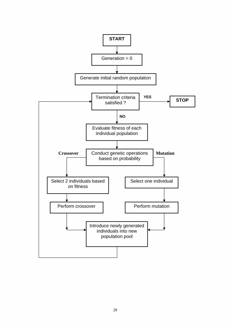
The basic procedure of GP, Fig. 2, can be described as follows:

1. generate the set of initial population;

2. evaluate each parse tree and assign the fitness;

3. form the temporary population by selecting candidates according to their fitness.

This temporary population is called the mating pool. Candidates with higher

fitness are given greater probabilities to mate and hence, to produce children or

offspring;

4. choose pairs of parse tree from the temporary mating pool randomly for mating

and apply the genetic operator called crossover. Crossover is the exchange of

genetic material (such as fitness, composition) between two selected candidates;

5. select a crossover site where the material will be exchanged randomly, thereby

resulting in the creation of offspring;

6. apply another genetic operator known as mutation which randomly changes the

genetic information of the candidate;

7. copy the resultant chromosomes into the new population;

8. evaluate the performance of the new population;

9. repeat steps 3-8 until a predetermined criterion is reached.

Selection, Crossover and Mutation

Selection is the process of altering the fitness of the individual with respect to

the whole generation's average performance. This is an important step because it

determines directly the individual's chances of its representation in the next

generation. A common selection method is fitness ranking. Individuals are sorted

6

according to the fitness values and ranked accordingly. Another selection method is

the tournament selection. This method fills the mating pool without the need of fitness

mapping. Pairs of individuals are picked at random from the population. The

individual with a higher fitness value is copied into the mating pool directly. This is

repeated until the pool is filled.

Crossover is the first process of producing new individuals from the selected

individuals in the mating pool. It takes two individuals and prunes their branch at

some randomly chosen position, into two segments (Figure 3a). Exchanging the

segments produces two new possible solution sets (Figure 3b). The two new solution

sets or children inherit some characteristics from their parents and genetic information

is thereby exchanged in the process. As the process continues, the fitness of the whole

population increases and converges to finding the near optimal solution set.

Mutation is the random alteration of the individual parse tree at the branch or

node level (Figure 4). Mutation is a mechanism that perturbs the parse tree structure.

It does not usually change the tree structure but the information content in the parse

tree. It therefore explores a new domain and serves to free the search from the

possibility of being trapped in local optima. It should be noted that mutation can be

destructive, causing rapid degradation of relatively "fit" solution sets if the probability

of mutation is set too high. Depending on the strategy adopted, mutation rate can be

low according GA-type mutation or high according to ES-type mutation.

The genetic programming introduced here is one of the simplest forms

available. Instead of Polish notations, GP solution sets can also be represented in other

forms such as: direct acylic graphs (Handley, 1994), linear representation (Perkis,

1994) and direct graphs (Poli, 1996). The evolution processes can also vary such as

using automatically defined functions (Koza, 1994), and adaptive representation

7

through learning (Rosca and Ballard, 1996), etc. These details can be found, for

example, in Koza (1992, 1994), Kinnear (1994), Angeline and Kinnear (1996) and

Langdon (1998).

AN EXAMPLE OF GENETIC SYMBOLIC REGRESSION

An example is shown here to illustrate the concept of GSR. The problem of

interest is to infer the Bernoulli equation for a steady, 1-dimensional fluid flow:

constg

vpzE =++=

2

2

γ(1)

where z = vertical distance above a datum (m)p = pressure (N/m2)v = velocity (m/s)g = Earth’s gravitational acceleration (9.81 m/s2)γ = specific gravity of water (9810 N/m3)

From Eq.(1), 1000 sets of different combinations of z, p and v are generated using a

standard random number generator. The values of the energy head, E, are then

computed correspondingly. It should be noted that this example was used in Maarten

and Babovic (1999) where problems involving variables of different dimensions are

discussed. For example, if variable z were to be multiplied with variable v, then the

resulting expression has a dimension of square-of-length/time which is inconsistent

with the dimension of variable E (length). In their paper, such occurrences of

dimensional inconsistency are penalized, to ensure dimensional consistency of the

resulting GP expression.

In this study, however, to circumvent the problem of dimension inconsistency,

each of the values of z, p and v is normalized or non-dimensionalized by using each

variable’s maximum value. By doing so, Eq.(1) is then transformed to a new form:

constg

vvppzzEE =++=

2

2max

2max

maxmax

γ(2)

8

or

constvCpCzCE =++= 2321

(3)

where the non-dimensionalized variables are given by:

maxE

EE =

(4a)

maxz

zz =

(4b)

maxp

pp =

(4c)

maxv

vv =

(4d)

and the coefficients are:

max

max1 E

zC = (5a)

max

max2 .E

pC

γ= (5b)

max

2max

3 .2 Eg

vC = (5c)

The terminal set used is the set of non-dimensionalized variables { }vpz

,,

while the functional set is {+, -, /, *}. Crossover is performed by randomly choosing

the sub-tree insertion location. The objective function is to find the minimum of the

root mean square error (RMSE) of the predicted energy head. The other GP relevant

parameters and their values are shown in Table 1. The genetic programming software

used in this study is GPkernel developed at the Danish Hydraulic Institute. The initial

population is generated by a random number generator. The size of the tree of the

initial population is constrained to a maximum of fifteen levels and the subsequent

tree size is constrained to forty-five levels. This restriction is necessary since GP has

the tendency to infer a Fourier expansion-type function if the tree size is not limited.

9

This type of expansion, although it may fit the data very well, does not add value in

the function interpretation.

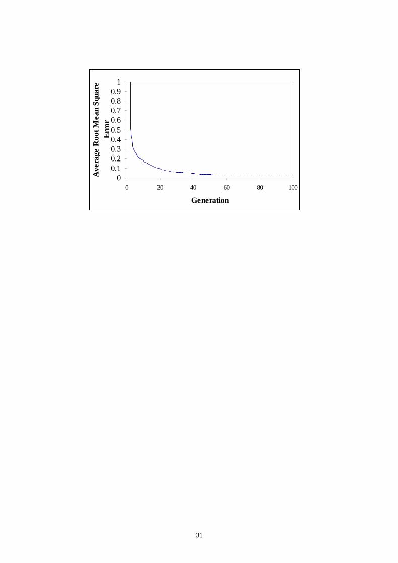
Ten different runs are performed, each using a different seed, to generate the

random numbers. Each time GPkernel is run for 15 minutes. Fig. 5 shows the average

root mean square error (RMSE) of each generation in the GSR runs. It should be

noted that the average RMSE, for all 10 runs, decreases rapidly as the generation

progresses and reached values near to zero for most of the runs. As a result, exact

formulae (up to 3 significant figures) are produced from each run.

The above simple example illustrates the capability of GP, or GSR technique

to infer the correct functional relationship when there are no errors in the raw data.

The next section illustrates the use of GSR as a new updating procedure combined

with rainfall runoff simulation models.

GP APPLICATION IN REAL-TIME RUNOFF FORECASTING

A forecasting system is a system that takes information on the past and current

states of meteorological conditions and those of the catchment, as inputs to it, and

forecasts the catchment’s response into the future. In real-time forecasting, however,

the originally forecast values may be updated or modified as measured data become

available and, thus, prediction errors can be determined and used for forecasting. In

real-time runoff forecasting with rainfall runoff simulation models, rainfall time series

up to the desired runoff forecast horizon must be available. The required rainfall time

series within the runoff forecast horizon may be estimated with, for example, a non-

linear prediction method. In this study, the measured rainfall time series, at any runoff

forecast horizon, is made available to evaluate the performance of the proposed GSR

based error updating scheme.

10

The focus of this study is to: (1) compare the forecasts of a calibrated rainfall-

runoff model, e.g. NAM, with and without the GSR based error updating scheme; and

(2) suggest how far in the future, i.e. the maximum forecast horizon, the GSR based

error updating scheme can be used with confidence.

The catchment simulation model used in this study is a lumped rainfall-runoff

model called Nedbor-Afstomnings-Model (NAM) which is presently part of the

MIKE11 software. The NAM model has been developed by the Hydrological Section

of the Institute of Hydrodynamics and Hydraulic Engineering at the Technical

University of Denmark (Nielsen and Hansen, 1973). The model can be defined as a

deterministic, conceptual, lumped type model with moderate input data requirement.

The NAM model consists of a set of linked mathematical statements describing, in a

simplified quantitative form , the behaviour of the land phase of the hydrological

cycle. The input data requirements are the catchment size, precipitation, potential

evapo-transpiration and temperature. It operates by continuously accounting for the

moisture content in the snow zone, surface zone, sub-surface zone and groundwater

zone storage. The model can be calibrated using historical data by adjusting one or

more of the seventeen parameters.

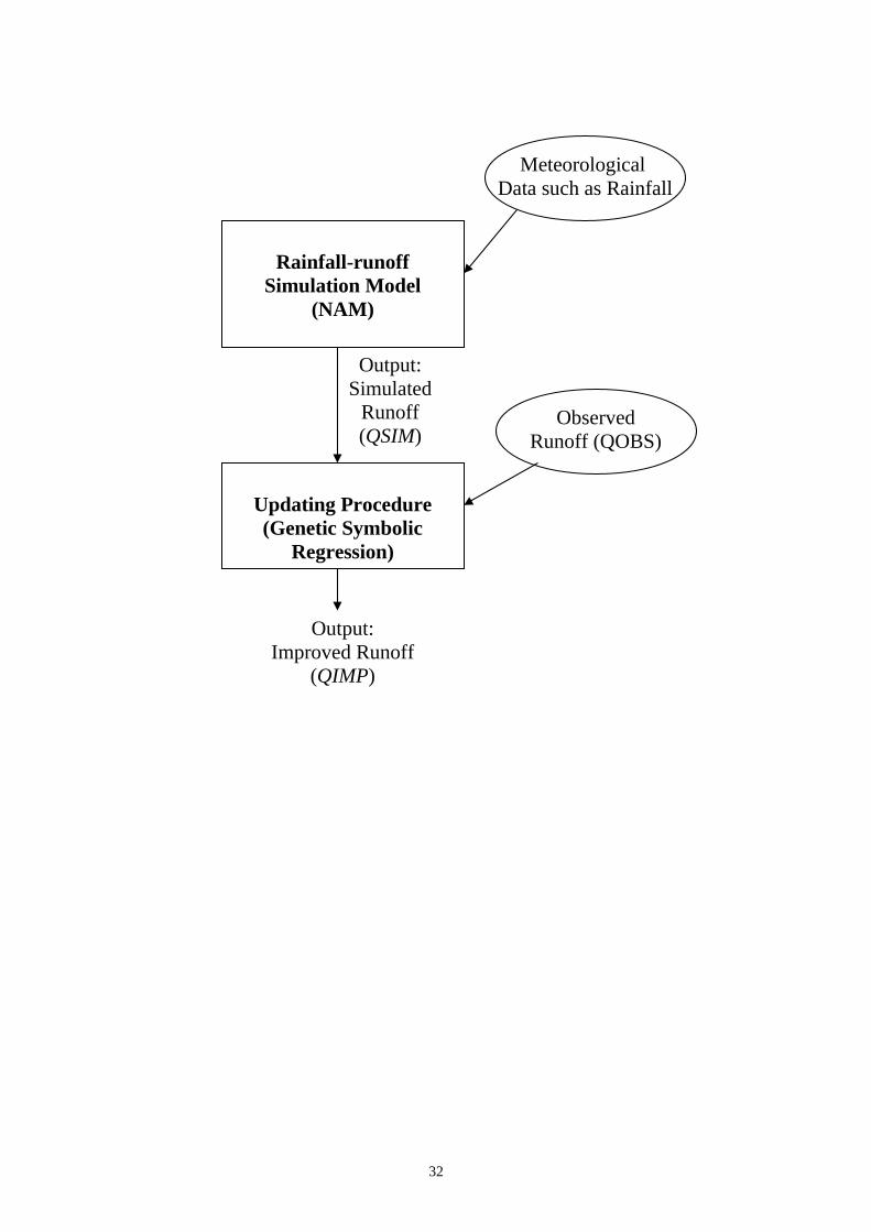
Figure 6 shows the schematic diagram of the proposed error updating using

GSR. The NAM model is first used to simulate the discharge, QSIM, for the whole

period of interest based on the rainfall data, R. The proposed procedure is then used

to compute the prediction error, ε, by comparing the simulated discharge, QSIM, with

the observed discharge, QOBS, for time, t. The new simulated or improved discharge,

QIMPt, is computed by adjusting QSIMt for each forecast lead-time within the forecast

horizon.

11

Mathematically, the measured discharge, QOBSt, at time t, can be expressed

as:

QOBSt = QSIMt + εt (6a)

or

εt = QOBSt - QSIMt (6b)

GSR is used to infer the functional relationship, F( ), between the simulated

discharges and the past simulation errors, and the present simulation error. For lead

time of 1 hour, the functional relationship for GSR prediction error, 1ˆ +tε , may be

expressed as follows:

{ }41411 ....,,....,,ˆ −−−++ = ttttttt QSIMQSIMQSIMF εεεε (7a)

and the forecast improved discharge, QIMPt+1, can be obtained from:

111 ˆ +++ += ttt QSIMQIMP ε (7b)

For lead time of 2, 3,…, α hours, the recursive form of Eq. (7) can be written as:

{ }414 ˆ,....,ˆ,,....,ˆ −+−+−+++ = ααααα εεε ttttt QSIMQSIMF (8a)

ααα ε +++ += ttt QSIMQIMP ˆ (8b)

QSIM and ε of the immediate past 5 time steps are included in the functional set since

the catchment’s time of concentration varies up to a maximum of 5 hours, i.e. 5 time

steps (WMO, 1992).

It should be noted that the values of αε +tˆ in Eq. (8a) may be either the actual

errors at instances when measured data are available or GSR derived errors.

The real-time flood forecasting with updating procedure for a 1-hour lead-time could

be summarized as follows:

12

1. The NAM model is first calibrated using an automatic calibration routine, e.g.

Accelerated Convergence Genetic Algorithm, ACGA (Liong et al., 1998), on the

entire runoff period from 1972-1974;

2. The prediction errors, denoted by ε, between the NAM simulated and observed

runoff for each time interval, are computed;

3. Ten storm events, representing high flow regimes with minimum discharge of 4

m3/s, are selected from the calibration runoff period, for the symbolic regression

using GP. This minimum discharge criterion is also used in the selection of the

verification data set;

4. GSR is then used to derive the functional relationship between the present

prediction error, ε̂ , and the NAM simulated discharge, QSIM, and the past

prediction errors, ε, as given in Eq. (7a);

5. The improved simulated discharge, QIMP, is finally calculated, using Eq. (7b) and

compared with the measured discharge.

For α > 1, the above procedure is repeated following Eqs. (8a) and (8b).

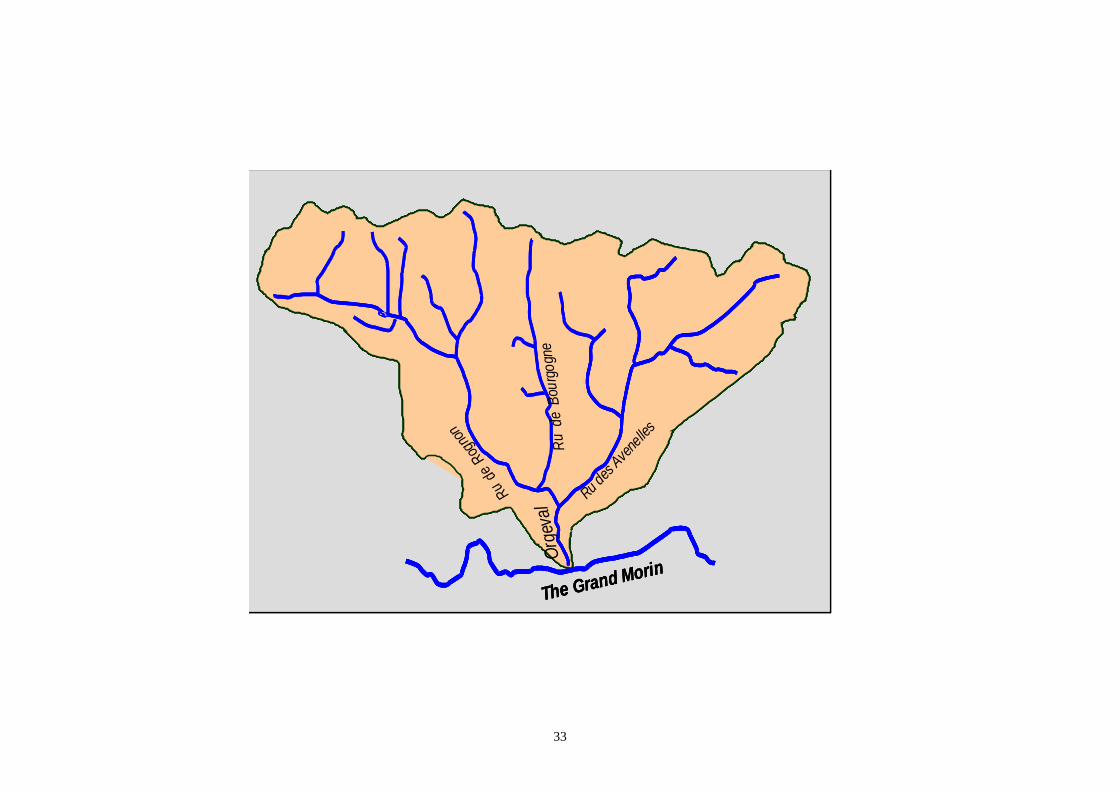
In this study, the catchment under consideration is the Orgeval catchment, in France

(Fig. 7), which has been studied extensively in the World Meteorological

Organization’s inter-comparison project (WMO, 1992). The catchment is located

about 80 km east of Paris and the main river that drains the catchment runoff is the

Orgeval. The catchment has an area of about 104 km2. The catchment comprises

mainly rural area, with only 1 percent of the total area urban and 18 percent of the

total area forest.

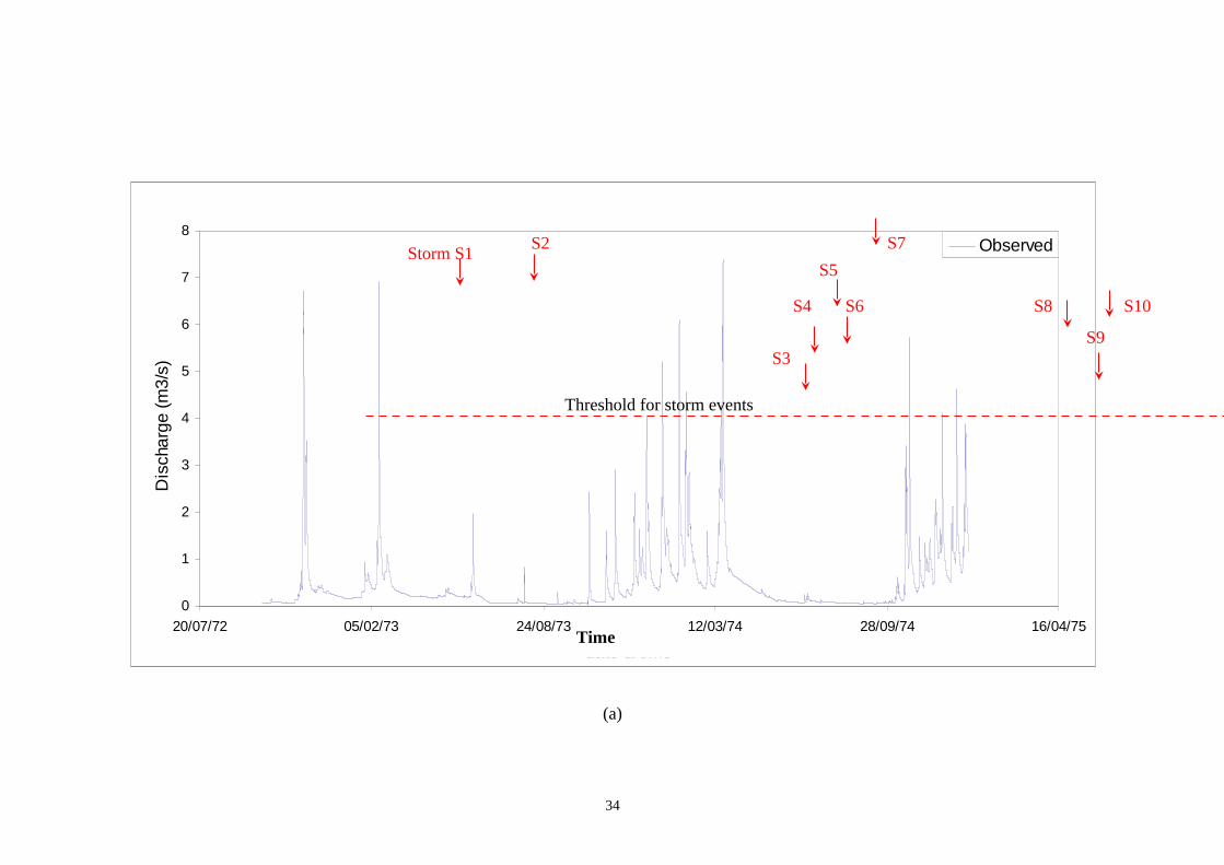
In this study, a total of ten storm events (denoted as storms S1 – S10) from a

1972 – 1974 hourly flow record was selected for training the GSR (Fig. 8(a)) while a

total of six storm events (denoted as storms S11 – S16) between 1979 –1980 (Fig. 8

13

(b)) was selected and used for the verification of the updating procedure. Fig. 9(a) and

9(b) show the observed and NAM simulated hydrographs for two of the selected GSR

training events. These ten storm events represent high flow regimes which are the

focus of GSR training in this study. It should be noted that the maximum peak

discharge of the GSR training storms is 7.38 m3/s while those of the verification storm

events range from 10 m3/s to 29 m3/s.

Following the example in the previous section, both the dependent

variable, ε̂ , and the independent variables, QSIM and ε, are non-

dimensionalized using their respective maximum values. Hence, the terminal set

in GSR for the 1-hr lead time, for example, is given by the normalized values

{ }541 ...,,,...,,, −−− ttttt QSIMQSIMQSIM εε and the functional set is given

by the basic algebraic operators {+, -, *, / }. Henceforth, all variables used in the

study are normalized variables and the bar sign on each variable is therefore

suspended. The objective function searches the minimum of the root mean square

error (RMSE) of the predicted error, ε̂ . In this study, the GP program, GPKernel,

was run for 30 minutes on a Pentium II 300 PC. The other GP relevant parameters and

their values are shown in Table 2. The population size of the parent and children are

both set at 3000. It is to be noted that, from various runs attempted, it was difficult to

achieve good prediction accuracy with a smaller population size.

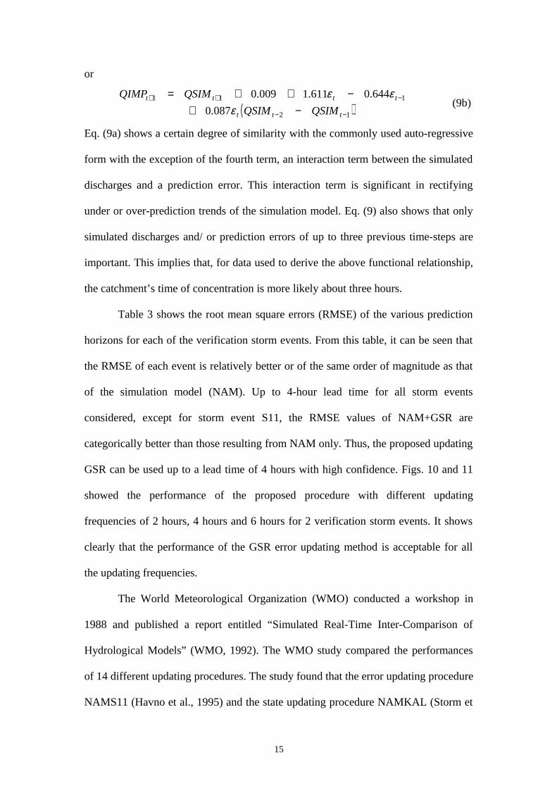
Discussion and Analysis of Results

The best functional form, with the minimum RMSE, resulting from GSR is as

follows:

( )12

11

087.0

644.0611.1009.0ˆ

−−

−+

−+−+=

ttt

ttt

QSIMQSIMεεεε

(9a)

14

or

( )12

111

087.0

644.0611.1009.0

−−

−++

−+−++=

ttt

tttt

QSIMQSIM

QSIMQIMP

εεε

(9b)

Eq. (9a) shows a certain degree of similarity with the commonly used auto-regressive

form with the exception of the fourth term, an interaction term between the simulated

discharges and a prediction error. This interaction term is significant in rectifying

under or over-prediction trends of the simulation model. Eq. (9) also shows that only

simulated discharges and/ or prediction errors of up to three previous time-steps are

important. This implies that, for data used to derive the above functional relationship,

the catchment’s time of concentration is more likely about three hours.

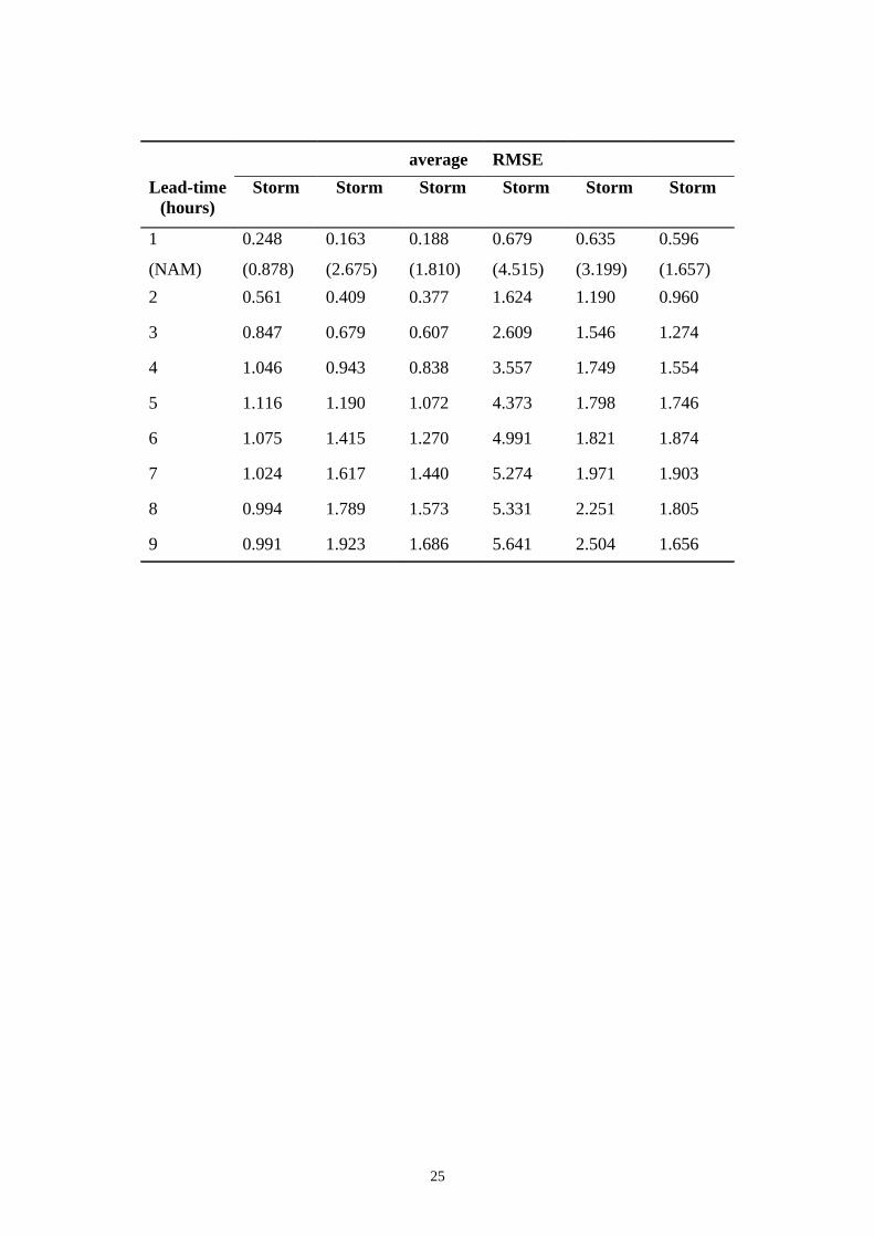
Table 3 shows the root mean square errors (RMSE) of the various prediction

horizons for each of the verification storm events. From this table, it can be seen that

the RMSE of each event is relatively better or of the same order of magnitude as that

of the simulation model (NAM). Up to 4-hour lead time for all storm events

considered, except for storm event S11, the RMSE values of NAM+GSR are

categorically better than those resulting from NAM only. Thus, the proposed updating

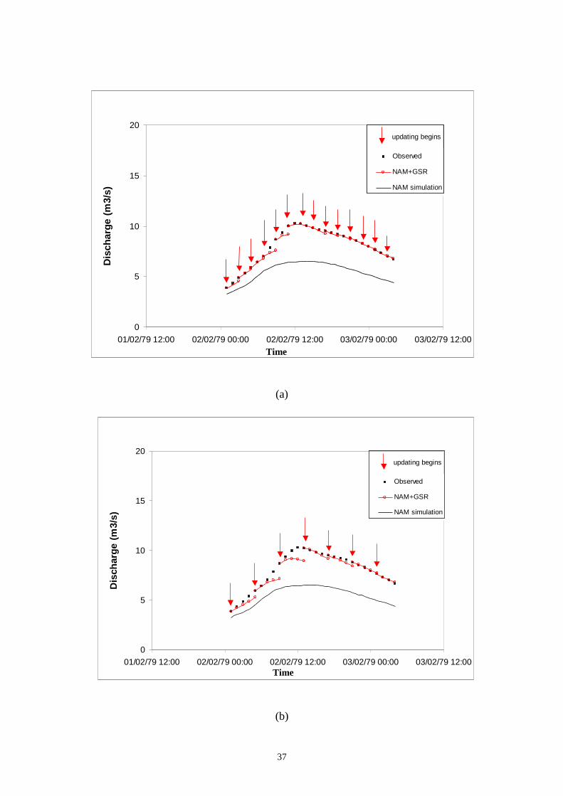
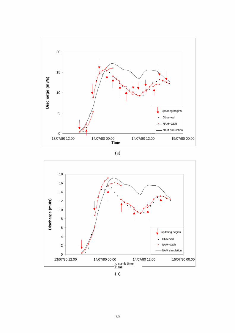
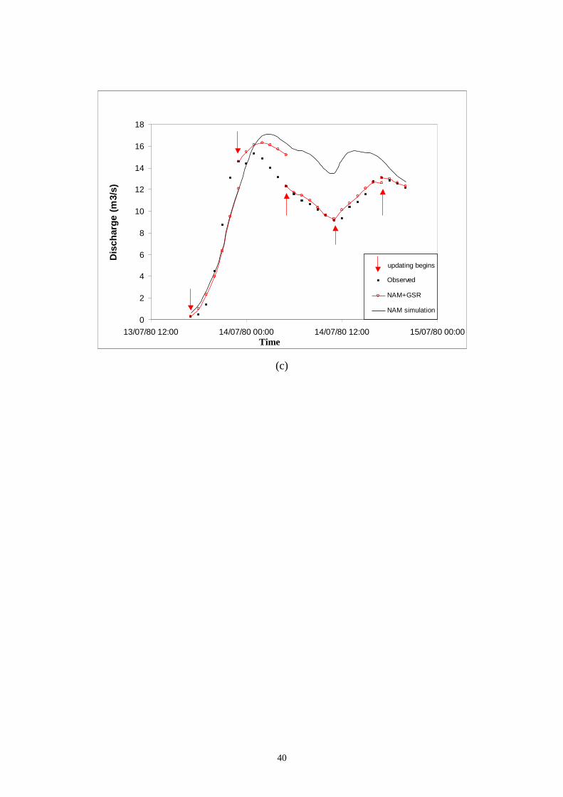
GSR can be used up to a lead time of 4 hours with high confidence. Figs. 10 and 11

showed the performance of the proposed procedure with different updating

frequencies of 2 hours, 4 hours and 6 hours for 2 verification storm events. It shows

clearly that the performance of the GSR error updating method is acceptable for all

the updating frequencies.

The World Meteorological Organization (WMO) conducted a workshop in

1988 and published a report entitled “Simulated Real-Time Inter-Comparison of

Hydrological Models” (WMO, 1992). The WMO study compared the performances

of 14 different updating procedures. The study found that the error updating procedure

NAMS11 (Havno et al., 1995) and the state updating procedure NAMKAL (Storm et

15

al., 1988) yielded best performance on the French Orgeval catchment. Briefly,

NAMS11 applies: (1) NAM rainfall-runoff simulation model and the MIKE11

hydrodynamic module; and (2) an error correction technique based on a first order

autoregressive model. NAMKAL is a modified NAM model, reformulated in state

space form and updated with an extended Kalman filtering algorithm.

In the WMO study, forecasts were updated at every 4th-hour. Thus, their

results are now compared with this study’s proposed GSR based updating scheme of

4-hour runoff forecast horizon. The choice of the updating interval coincides with the

earlier drawn conclusion from Table 3. Figure 12(a) and (b) shows the average

RMSE, of two verification storm events (storms S12 and S15) resulting from various

updating schemes, NAM+GSR, NAMS11 and NAMKAL. These two storm events

are the same as those chosen in Figs. 10 and 11. Fig. 12(a) shows that for storm event

S12, the proposed NAM+GSR performs better in the first 3 hours than NAMS11 and

NAMKAL while on the fourth hour, they all perform equally. Fig. 12(b), however,

shows clearly that for storm event S15, the NAM+GSR is categorically better than the

two other techniques.

16

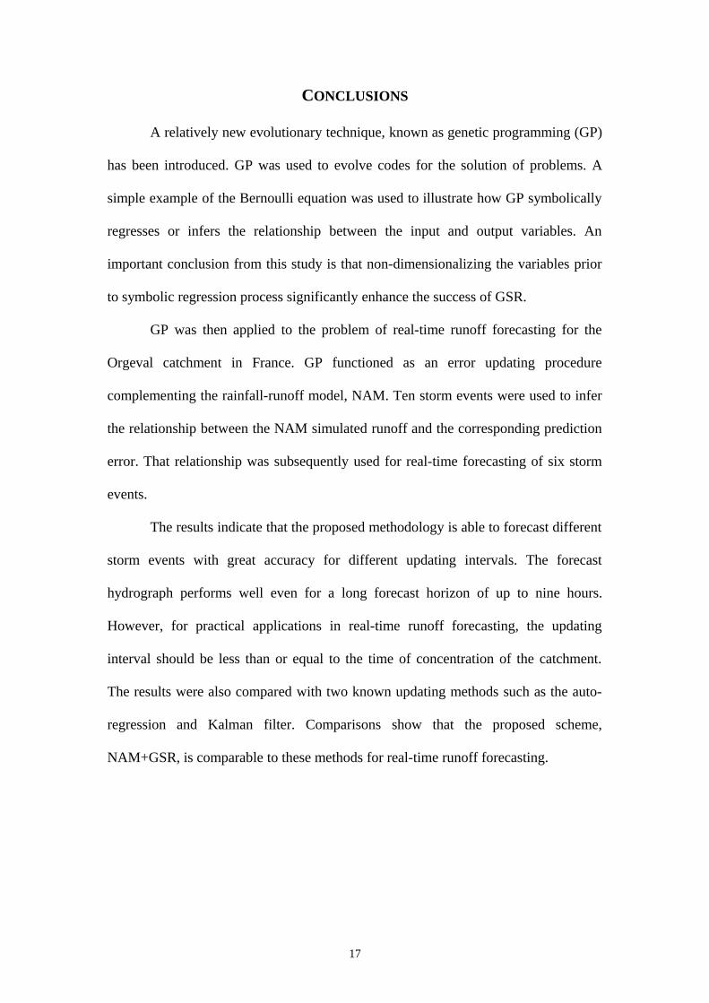
CONCLUSIONS

A relatively new evolutionary technique, known as genetic programming (GP)

has been introduced. GP was used to evolve codes for the solution of problems. A

simple example of the Bernoulli equation was used to illustrate how GP symbolically

regresses or infers the relationship between the input and output variables. An

important conclusion from this study is that non-dimensionalizing the variables prior

to symbolic regression process significantly enhance the success of GSR.

GP was then applied to the problem of real-time runoff forecasting for the

Orgeval catchment in France. GP functioned as an error updating procedure

complementing the rainfall-runoff model, NAM. Ten storm events were used to infer

the relationship between the NAM simulated runoff and the corresponding prediction

error. That relationship was subsequently used for real-time forecasting of six storm

events.

The results indicate that the proposed methodology is able to forecast different

storm events with great accuracy for different updating intervals. The forecast

hydrograph performs well even for a long forecast horizon of up to nine hours.

However, for practical applications in real-time runoff forecasting, the updating

interval should be less than or equal to the time of concentration of the catchment.

The results were also compared with two known updating methods such as the auto-

regression and Kalman filter. Comparisons show that the proposed scheme,

NAM+GSR, is comparable to these methods for real-time runoff forecasting.

17

ACKNOWLEDGMENTS

The work is sponsored jointly by the National University of Singapore

research project, RP3972705 and the Talent Project No 9800463 “Data to Knowledge

- D2K” funded by the Danish Technical Research Council (STVF). Part of the work

was done by the first author during his study leave at Danish Hydraulic Institute

(DHI).

18

LITERATURE CITED:

Angeline, P. J. and Kinnear, K. E., (1996). Advances in Genetic Programming 2. MIT

Press, Cambridge, MA.

Babovic, V. and Abbott, M. B., (1997). The evolution of equations from hydraulic

data, part II: applications. Journal of Hydraulic Research, 35(3): 411-430.

Fogel, L. J., Owens, A. J. and Walsh, M. J., (1966). Artificial Intelligence through

Simulated Evolution. John Wiley, New York.

Handley, S., (1994). On the use of a directed acyclic graph to represent a population

of computer programs. In Proceedings of the 1994 IEEE World Congress on

Computational Intelligence. IEEE Press, pp. 154-159.

Holland, J. H., (1975). Adaptation in Natural and Artificial Systems, University of

Michigan Press, Ann Arbor, 1975.

Kinnear, K. E., (1994). Advances in Genetic Programming. The MIT Press,

Cambridge, MA.

Koza, J. R., (1992). Genetic Programming: On the Programming of Computers by

Means of Natural Selection. The MIT Press, Cambridge, MA.

Koza, J. R., (1994). Genetic Programming 2: Automatic Discovery of Reusable

Programs. The MIT Press, Cambridge, MA.

Langdon, W. B., (1998). Genetic Programming and Data Structures. Kluwer

Academic Publishers, Norwell, MA.

Lee, G. Y. and Suzuki, A., (1995). Genetic programming approach for time series

analysis and prediction. Journal of Graduate School and Faculty of Engineering,

University of Tokyo (B), 43(2): 201-220.

Liong, S. Y., Khu, S. T. and Chan, W. T., (1998). Derivation of Pareto front with

accelerated convergence genetic algorithm, ACGA. In Proceedings of the 3rd

19

International Conference on Hydroinformatics, Babovic, V. and Larsen, L. C.

(eds.), Volume 2, pp. 889 - 897.

Lukasiewicz, J., (1957). Aristotle's Syllogistic from the Standpoint of Modern Formal

Logic. Oxford , Clarendon Press.

Maarten, K. and Babovic, V., (1999). Dimensionally Aware Genetic Programming.

Proceedings of the Genetic and Evolutionary Computation Conference,

GECCO-99, Daida, W. B., Eiben, A. E., Garzon, M. H., Honavar, V., Jakiela,

M. and Smith, R. E. (eds.), Morgan Kaufmann, CA.

Nielsen, S. A. and Hansen, E., (1973). Numerical simulation of rainfall runoff process

on a daily basis. Nordic Hydrology, 4: 171-190.

Oakley, N. and Howard, E., (1994). The application of genetic programming to the

investigation of short, noisy, chaotic data series. In Evolutionary Programming,

Lecture Notes in Computer Sciences, Fogarty, T C. (ed.), No. 865, Springer-

Verlag, Germany, pp. 320-332.

Perkis, T., (1994). Stack-based genetic programming. In Proceedings of the 1994

IEEE World Congress on Computational Intelligence, Vol. 1, IEEE Press, pp.

148-153.

Poli, R., (1996). Parallel distributed genetic programming. Technical Report CSRP-

96-15, School of Computer Science, University of Birmingham.

Rosca, J. P. and Ballard, D. H., (1996). Discovery of subroutines in genetic

programming. In Advances in Genetic Programming 2, Angeline, P. J. and

Kinnear, K. E. (eds.), The MIT Press, Cambridge, MA., pp. 177-202.

Rungo, M., Refgaard, J. C. and Havno, K., (1991). The updating procedure in the

MIKE11 modelling systme for real-time forecasting. Proceeding of the

20

International Symposium on Hydrological Applications on Weather Radar, Ellis

Horword publication, University of Salford, 14-17 August 1989, pp. 497-508.

Schwefel, H. P., (1981). Numerical Optimization of Computer Models. John Wiley,

Chichester.

Storm, B., Jensen, K. H. and Refgaard, J. C., (1988). Estimation of catchment rainfall

uncertainty and its influence on runoff prediction. Nordic Hydrology, Vol. 19,

pp. 77-88.

Whigham, P. A. and Crapper, P. F., (1999). Modelling Rainfall-runoff Relationships

using Genetic Programming. Special Issue of Journal of Mathematical and

Computer Modelling (in press).

WMO, (1992). Simulated Real-Time Inter-Comparison of Hydrological Models.

WMO Operational Hydrology Report no. 38, WMO no. 779. World

Meteorological Organization, Geneva.

21

List of Tables:

Table 1 : Genetic Programming Parameters Used in Bernoulli Equation

ExampleTable 2 : Genetic Programming Parameters Used in Real-time Runoff

Forecasting ExampleTable 3 : Root Mean Square Error of Testing Storms for Different Prediction

Lead-times

22

Parameter ValueSize of parent 1000Size of children 1000Tournament size 3Crossover rate 1.0Mutation rate 0.3Maximum initial tree size 15Maximum tree size 45

23

Parameter ValueSize of parent 3000Size of children 3000Tournament size 3Crossover rate 1.0Mutation rate 0.3Maximum initial tree size 15Maximum tree size 30

24

average RMSE

Lead-time(hours)

Storm Storm Storm Storm Storm Storm

1

(NAM)

0.248

(0.878)

0.163

(2.675)

0.188

(1.810)

0.679

(4.515)

0.635

(3.199)

0.596

(1.657)

2 0.561 0.409 0.377 1.624 1.190 0.960

3 0.847 0.679 0.607 2.609 1.546 1.274

4 1.046 0.943 0.838 3.557 1.749 1.554

5 1.116 1.190 1.072 4.373 1.798 1.746

6 1.075 1.415 1.270 4.991 1.821 1.874

7 1.024 1.617 1.440 5.274 1.971 1.903

8 0.994 1.789 1.573 5.331 2.251 1.805

9 0.991 1.923 1.686 5.641 2.504 1.656

25

List of Figures

Figure 1 : Different Forms of Representation in Genetic ProgrammingFigure 2 : Basic Procedure of Genetic ProgrammingFigure 3 : Crossover in Genetic ProgrammingFigure 4 : Mutation in Genetic ProgrammingFigure 5 : Rapid Convergence of GSR for Bernoulli Equation ExampleFigure 6 : Schematic Diagram of Updating ProcedureFigure 7 : Location of Orgeval CatchmentFigure 8 : Hydrographs of (a)Training and (b)Verification Storm EventsFigure 9 : Comparison of Observed and Simulated Hydrographs for 2

Training Storm Events: (a) S2 and (b) S7Figure 10 : Updating Every α hours and Forecasting up to 6 hours for

Verification Storm Event S12: (a) α = 2 hours; (b) α = 4 hours;

and (c) α = 6 hoursFigure 11 : Updating Every α hours and Forecasting up to 6 hours for

Verification Storm Event S15: (a) α = 2 hours; (b) α = 4 hours;

and (c) α = 6 hoursFigure 12 : Average RMSE of 2 Verification Storm Events: (a) S12 and (b)

S15

26

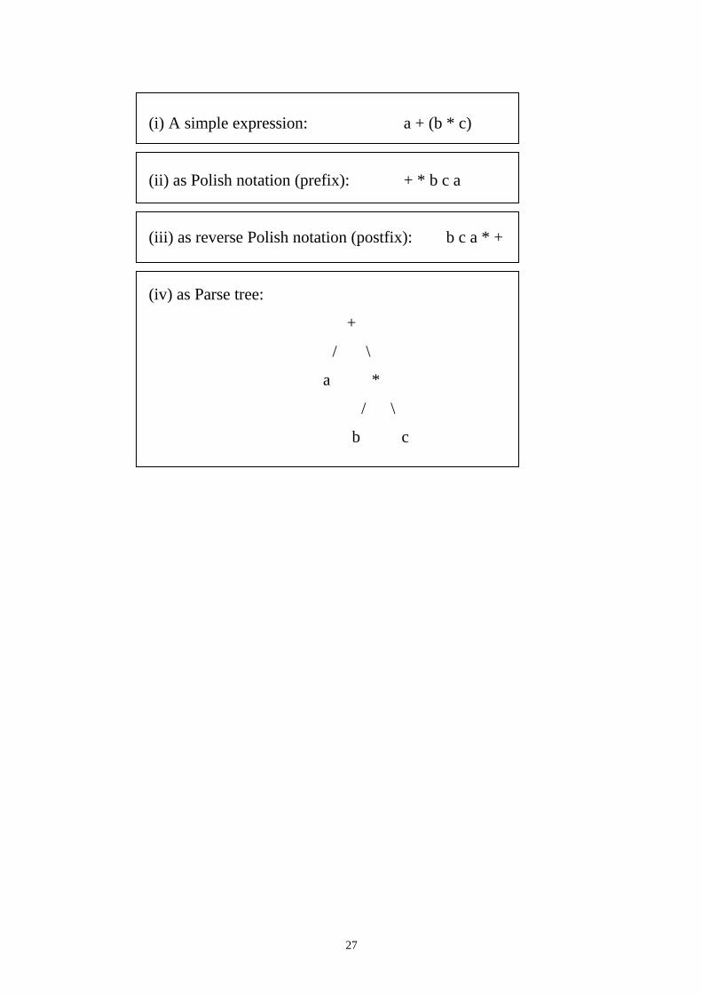
(i) A simple expression: a + (b * c)

(ii) as Polish notation (prefix): + * b c a

(iii) as reverse Polish notation (postfix): b c a * +

(iv) as Parse tree:

+

/ \

a *

/ \

b c

27

28

START

Generation = 0

Generate initial random population

Termination criteria satisfied ?

NO

Evaluate fitness of each individual population

YESSTOP

Conduct genetic operations based on probability

Select 2 individuals based on fitness

Perform mutation

Select one individual

Perform crossover

Introduce newly generated individuals into new

population pool

Crossover Mutation

Parent 1 Parent 2

Direct algebraic form:. a+(b*c) (b+a)*((a*c)-d)

(a)

Child 1 Child 2

Direct algebraic form:. a+((a*c)-d) (b+a)*b*c

(b)

29

+

*

b

a

c

*

-

*

+

dab

a c

+

a *

b c

*

+

ab

-

* d

a c

a + (b * c) a + (b / c)

30

+

*

b

a

c

+

/

b

a

c

Mutation

31

00.10.20.30.40.50.60.70.80.9

1

0 20 40 60 80 100

Generation

Ave

rage

Roo

t M

ean

Squ

are

Err

or

32

Rainfall-runoff Simulation Model

(NAM)

Meteorological Data such as Rainfall

Updating Procedure(Genetic Symbolic

Regression)

ObservedRunoff (QOBS)

Output: Simulated

Runoff(QSIM)

Output:Improved Runoff

(QIMP)

The Grand Morin

Ru de

Rog

non

Ru

de B

ourg

ogne

Ru des A

vene

lles

Org

eval

The Grand Morin

Ru de

Rog

non

Ru

de B

ourg

ogne

Ru des A

vene

lles

Org

eval

The Grand Morin

Ru de

Rog

non

Ru

de B

ourg

ogne

Ru des A

vene

lles

Org

eval

The Grand Morin

Ru de

Rog

non

Ru

de B

ourg

ogne

Ru des A

vene

lles

Org

eval

The Grand Morin

Ru de

Rog

non

Ru

de B

ourg

ogne

Ru des A

vene

lles

The Grand Morin

Ru de

Rog

non

Ru

de B

ourg

ogne

Ru des A

vene

lles

Org

eval

33

(a)

0

1

2

3

4

5

6

7

8

20/07/72 05/02/73 24/08/73 12/03/74 28/09/74 16/04/75

date & time

Dis

cha

rge

(m

3/s

)

ObservedS2

S3

Storm S1

S6S4

S5

S8

S7

S9

S10

Threshold for storm events

Time

34

(b)

Validation data

0

5

10

15

20

25

30

35

11/06/78 02/04/79 05/05/79 08/03/79 11/01/79 01/30/80 04/29/80 07/28/80

Date

Dis

ch

arg

e (

m3

/s)

Threshold for storm event

Storm S11

S12S13

S14

S15

S16

Time

35

(a)

(b)

Storm event 2 (Calibration)

3

4

5

6

7

8

12/02/73 12:00 13/02/73 00:00 13/02/73 12:00 14/02/73 00:00 14/02/73 12:00

date & time

Dis

ch

arg

e (

m3

/s)

Observed

NAM

Storm event 7 (Calibration)

3

4

5

6

7

8

20/03/74 00:00 21/03/74 00:00 22/03/74 00:00 23/03/74 00:00

date & time

Dis

ch

arg

e (m

3/s)

Observed

NAM

Time Time

36

(a)

(b)

0

5

10

15

20

01/02/79 12:00 02/02/79 00:00 02/02/79 12:00 03/02/79 00:00 03/02/79 12:00date & time

Dis

char

ge

(m

3/s)

Observed

NAM+GSR

NAM simulation

updating begins

0

5

10

15

20

01/02/79 12:00 02/02/79 00:00 02/02/79 12:00 03/02/79 00:00 03/02/79 12:00date & time

Dis

char

ge

(m

3/s)

Observed

NAM+GSR

NAM simulation

updating begins

Time

Time

37

(c)

0

5

10

15

20

01/02/79 12:00 02/02/79 00:00 02/02/79 12:00 03/02/79 00:00 03/02/79 12:00date & time

Dis

char

ge

(m

3/s)

Observed

NAM+GSR

NAM simulation

updating begins

Time

38

(a)

(b)

0

5

10

15

20

13/07/80 12:00 14/07/80 00:00 14/07/80 12:00 15/07/80 00:00date & time

Dis

char

ge

(m

3/s

)

Observed

NAM+GSR

NAM simulation

updating begins

0

2

4

6

8

10

12

14

16

18

13/07/80 12:00 14/07/80 00:00 14/07/80 12:00 15/07/80 00:00date & time

Dis

cha

rge

(m

3/s

)

Observed

NAM+GSR

NAM simulation

updating begins

Time

Time

39

(c)

0

2

4

6

8

10

12

14

16

18

13/07/80 12:00 14/07/80 00:00 14/07/80 12:00 15/07/80 00:00date & time

Dis

char

ge

(m

3/s)

Observed

NAM+GSR

NAM simulation

updating begins

Time

40

(a)

(b)

Storm Event S15

0.0

1.0

2.0

3.0

4.0

5.0

0 1 2 3 4 5

Forecast lead time [hrs]

RM

SE

[m

3/s]

NAM without updating

GP+GSR

NAMS11

NAMKAL

Storm Event S12

0.0

0.5

1.0

1.5

2.0

2.5

3.0

0 1 2 3 4 5

Forecast lead time [hrs]

RM

SE

(m

3/s)

NAM without updating

GP+GSR

NAMS11

NAMKAL

41