THE GENERALIZED QUANTUM DATABASE SEARCH

THE GENERALIZED QUANTUM DATABASE SEARCH

ALGORITHM

SANDOR IMRE, FERENC BALAZS

Abstract. In this paper we present a generalized description of the Grover

operator, employed in a quantum database search algorithm. We will discuss

the relation between the original and generalized operators as well as we will

show the optimal setting of parameters used in the Grover operator leading to

a single iteration during a database search.

1. Introduction

L. K. Grover published his fast database searching algorithm first in [1] and [2]using the diffusion matrix approach to illustrate the effect of the Grover operator,that took O(

√N ) iterations to carry out the search, which is the optimal solution,

as it was proved in [3]. Boyer , Brassard, Hoyer and Tapp [4] enhanced the originalalgorithm for more than one marked entry in several number of identical solutions inthe database and introduced upper bounds for the required number of evaluations.

After a short debate Bennett, Bernstein, Brassard and Vazirani gave the firstproof of the optimality of Grover’s algorithm in [5]. The proof was refined by Zalkain [6].

Later the rotation in two dimensional state space (with the bases of separatelysuperpositioned marked and unmarked states) SU(2) approach were introduced byAharonov in [7]. Within this book we followed this representation form accordingto its popularity in the literature.

During the above mentioned evolution of the Grover algorithm a new queststarted to formulate the building blocks of the algorithm as generally as possible.The motivations for putting so much effort into this direction were on one hand toget a much deeper insight into the heart of the algorithm and on the other hand toovercome the main shortcoming of the algorithm, namely the sure success of findinga marked state can not be guaranteed. In [8] the authors replaced the Hadamardtransformation with an arbitrary unitary one. The next step was the introductionof arbitrary phase rotations in the Oracle and the phase shifter instead of π in[9]. To provide sure success at the final measurement Brassard at all [10] run theoriginal Grover algorithm, but for the final turn a special Grover operator Groveroperator with smaller step was applied. Hoyer et al. [11] gave another ingenioussolution of the problem. They modified the original Grover algorithm and the initialdistribution.

To give another viewpoint Long at al introduced the three dimensional SO(3)picture in description of Grover operator in [12]. The achievements were summa-rized and extended by Long [13] and an exact matching condition was derived for

Key words and phrases. Grover’s Algorithm, Quantum computing, Quantum Signal Process-ing, Grover database search, generalized Grover Operator.

1

2 SANDOR IMRE, FERENC BALAZS

multiple marked states in [14]. Unfortunately the SO(3) picture is less picturesqueand it misses the global phase factor before the measurement. In normal case itdoes not cause any difficulty because measurement results are immune of it. How-ever, if it is planed (we plan) to reuse the final state of the index register withoutmeasurement as the input of a further algorithm (operator), it is crucial to dealwith the global phase. Therefore, Hsieh and Li [15] returned to the traditionaltwo dimensional SU(2) formulation and derived the same matching condition foeone marked element as Long achieved but they saved the final global phase factor.One important part of these solution, however, was missing. Namely, they requiredthat the initial sate should fit into the two dimensional state space defined by themarked and unmarked states. This gives large freedom for designers but encumberthe application of the generalized Grover algorithm as a building block of a largerquantum system.

Therefore another very important question within this topic proved to be theanalysis of the evolution of Grover’s algorithm when it is started from an arbitraryinitial state, i.e. the amplitudes are either real or complex and follow any arbitrarydistribution. In this case sure success can not be guaranteed, but the probability ofsuccess can be maximized. Biham and his team first gave the analysis of the originalGrover algorithm in [16], [17]. In [18] the analysis was extended to the generalizedGrover algorithm with arbitrary unitary transformation and phase rotations.

Within this paper we combined and enhanced the results for generalized Groversearch algorithm in terms of arbitrary initial distribution, arbitrary unitary trans-formation, arbitrary phase rotations and arbitrary number of marked items to builda method to construct an unstructured data base search algorithm which can beincluded inside a quantum computing system. Because its constructive nature thisalgorithm is capable to get any amplitude distribution at its input, provides suresuccess in case of measurement and allows to connect its output to another algo-rithm if no measurement is performed. Of course, this approach assumes that theinitial distribution is given and it determines all the other parameters according tothe construction rules. However, readers who are interested in applying a prede-fined unitary transformation as the fixed parameter should settle for a restrictedset of initial states and suggested to take a look at [15].

Grover´s data base search algorithm assumes the knowledge of the number ofmarked states, but it is typical that we do not have this information in advance.Brassard et al. [19] gives the first valuable idea how to estimate the missing numberof marked states, which was enhanced in [10] and traced back to a phase estimationof Grover operator.

A rather useful extension of the Grover algorithm when we decided to find min-imum/maximum point of a cost function. Durr and Hoyer suggested the first sta-tistical method and bound to solve the problem in [20]. Later based on this resultAhuya and Kapoor improved the bounds in [21]. A further beneficial exertion pos-sibilities of the Grover algorithm can be employed in Telecommunication field. Thepresent authors introduced the Grover database search based multiuser detectionin WCDMA environment in [22], [23], and [24].

Recently Grover emphasized in [25] that the number of elementary unitary op-erations can be reduced which lunched a new quest for the most effective Groverstructure in terms of number of basic operations.

THE GENERALIZED QUANTUM DATABASE SEARCH ALGORITHM 3

The rest of the paper is organized as follows. In Section 2. the original Groverquantum database search operator (G) is reviewed. In Section 4. we introduce thegeneralized Grover operator (Q) wherefor an example is shown in Section 5. Thepaper is closed with a final conclusion in Section 6.

2. Basic Grover Algorithm

Consider a large unsorted database, which contains N entries, to find the desiredvalue with any classical algorithms would need at least O(N ) steps.

2.1. The Searching Algorithm. Grover’s quantum searching algorithm (G) con-sists of four simple operations: an Oracle followed by a Hadamard-, a controlledphase-, and a Hadamard-transformation again, as depicted in Figure 1. In the nextsections we bring up the main behavior and functionality of G, apartly.

G

O

H Controlledphase shifter

H......

......

...

|q〉

|r〉

Figure 1. Sketch of Grover’s database search circuit

2.1.1. The Oracle. Let us consider a database with N = 2n entries, a quantumindex register |r〉 containing all the index values of the database in a quantumsuperposition and a black box, the so called Oracle. Grover’s gorgeous brainchildwas to implement a binary function f(x) in the Oracle, with the property

(1) f(x) =

1 if the entry belonging to index x matchesthe searched item

0 otherwise,

x = 0, 1, . . . , (N − 1). The function in (1) can have the value 1 either at a singleor multiple values of x, depending on how many identical searched entries in aparticular database exist. Entries, which are solutions for the search problem arecalled marked states according to the literature and ones which do not lead to asolution are referred as non marked states.

Invoking the Oracle (O) with the following computation rule (see Fig. 2) :

(2) |x〉|q〉 O7→ |x〉|q ⊗ f(x)〉,

where |x〉N and |q〉 =

(

|0〉−|1〉√2

)

are the wanted n = ldN qubit vector basis state

(i.e. the index in question) and an auxiliary one qubit state, respectively, the output


of the oracle will act as (see also the Deutsch-Jozsa algorithm in Sec. xx.)

|x〉( |0〉 − |1〉√

2

)

O7→

|x〉(

|0〉−|1〉√2

)

for x, whose entry

is not in the database

−|x〉(

|0〉−|1〉√2

)

for x whose entry

can be found in thedatabase,

or in more common compact mathematical form

(3) |x〉 O→ (−1)f(x)|x〉,where |q〉 does not change during the algorithm and can be neglected henceforth.

- - ?

f(x)

?

XOR- -

|q〉 = 1√2

(|0〉 − |1〉)

n qubit input |r〉

Figure 2. Inside in the Oracle O

The input state of the index register |r〉 feeded to the Oracle is assumed to bean equal superposition state of all the possible indexes

(4) |r〉 = |γ〉 , H⊗n |0〉n =1√N

N−1∑

x=0

|x〉,

where H⊗n

denotes the n-bit Hadamard-transformation whereas |0〉n = | 0 · · · 0︸︷︷︸

n

〉.

|γ〉 is depicted in Fig. 3. Let x = y denote the index of the marked entry, whoseamplitude is drawn with thick line in the figure.

-

6 6 6 6 66. . .

1√N

N︷︸︸︷

0 1 y N − 1x

Figure 3. The equal superposition input state |γ〉

Equation (3) can be interpreted as f(x) flips the sign of the amplitude of themarked state(s) and let the others unaltered (see Fig 4). One can express the


strategy of the Oracle according to the equation (4) in operator formalism such as

(5) O , I − 2|y〉〈y|,where (|y〉〈y|) stands for the outer product of marked state |y〉 as well as I denoteshere the N dimensional identity matrix.

- x

6 6

?

6 66. . .

1√N

N︷︸︸︷

Figure 4. The input state |γ〉 after invoking the Oracle

As an example, let the third state be marked (y = 2) in an n = 2 qubit quantum

index register, i.e. |y〉 =[0 0 1 0

]T. Substituting |y〉 into (5) the matrix Oy

representing the Oracle can be calculated as

Oy=2 = I − 2

0010

[0 0 1 0

]= I − 2

0 0 0 00 0 0 00 0 1 00 0 0 0

=

1 0 0 00 1 0 00 0 −1 00 0 0 1

,(6)

which corresponds to the amplitude flip depicted in Fig. 5.

2.1.2. Another phase reflection – Inversion about the average. The Oracle followedfirst by an n-dimensional Hadamard-gate (H), whose output qubits feed a Con-trolled Phase Shifter (P), defined as

P , (2|0〉〈0| − I) .

P changes the sign of all computational basis states except for x = 0. The finaloperation is again a Hadamard-gate (H). The Hadamard-gates and the controlledphase shifter inverts the output of the Oracle about its average. Hence the wholeGrover iteration can be formulated as

(7) G , HPHO = (2H|0〉〈0|H −HIH)O,where I refers to the N -dimensional identity operation again, which together withthe property of an unitary and Hermitian operator H = H† = H−1 simplifies HIHto I. Utilizing expressions (4) and (5), equation (7) becomes

(8) G = (2|γ〉〈γ| − I)O = (2|γ〉〈γ| − I) (I − 2|y〉〈y|) .Generally, the second phase rotation operation is denoted by Uγ = (2|γ〉〈γ| − I),

where |γ〉 =[

1/√N 1/

√N · · · 1/

√N]T

form (4), hence


Uγ = 2

1√N1√N...1√N

[1√N

1√N

· · · 1√N

]

− I

=

2N

− 1 2N

· · · 2N

2N

2N

− 1 · · · 2N

.... . .

...2N

· · · 2N

2N

− 1

.(9)

One may apply the operation Uγ on a vector |a〉 =[a0 a1 · · · aN−1

]Tand

observe the amplitude of the kth basis state

〈k|Uγ |a〉 = a02

N+ a1

2

N+ · · · +

(

ak2

N− ak

)

+ · · · +

+ aN2

N − 1=

= 21

N

N−1∑

i=0

ai − ak = 2a− ak,(10)

which denotes a subtraction of the yth amplitude from the two times of the averagea as it is depicted in Figure 5. The same observation is applied for every otherl = 0, . . . , N − 1, l 6= y components. In the figure y denotes the marked componentf(x)|x=y = 1, and l the undesired ones, where f(x)|x=l = 0, respectively. It isnoticeable, as a result of the inversion on the average a, the probability amplitudebelonging to wanted index y increases, whilst the amplitudes of other indexes falloff.

Invoking G several times, the algorithm amplifies the amplitude of the markedstate and suppresses those for unmarked ones. If the probability amplitude of themarked state takes the value 1, equivalently the values of others vanish, because∑

i |ai|2 = 1. This process is called in the quantum world ”Amplitude Amplifica-tion”. However, the basic Grover algorithm can not guarantee that we can reachexactly ay = 1.

6 6

?

6 66. . .

6

?

y

l

y′

l′

a

2a

Figure 5. Inversion of the amplitude of a marked index y and theunmarked one l on the average a


6 6 6 6. . .

6

6

y′

l′a

2a

Figure 6. Probability amplitudes of a marked component y andan unmarked one l after the Oracle operation

2.2. Required Number of Iterations Multiple Marked States. As we dis-cussed earlier amplitude amplification in Grover algorithm can not provide a suresuccess measurement of the marked index (i.e. ay = 1), because ay does not con-verge to 1, instead it is a periodical function of the iteration steps. For that reasonone should be able the predict the required number of iterations, which signifies:How many times should the Grover operator (G) be applied to get ay as close aspossible to 1? For this purpose we introduce a special geometrical description, bymeans we could also exploit an answer for databases with multiple marked entries(M > 1).

Let us form two basis state vectors from the marked and unmarked states as

|α〉 ,1√

N −M

∑

x∈S

|x〉,(11)

|β〉 ,1√M

∑

x∈S

|x〉,(12)

S : Set of marked indexes (f(x) = 1)

where (11) sums up the (N − M) states |x〉 that do not lead to a solution ofthe search problem and (12) does the same with M indexes |x〉 which lead to it.Variables M and N refer to the number of marked entries and the total number ofentries in the database, respectively.

6

-1

|α〉

|β〉

|γ〉

Ωγ

2

cos (Ωγ

2 )

sin (Ωγ

2 )

Figure 7. Projection of the initial state |γ〉 on the basis statevectors |α〉 and |β〉


The initial state of the index register |r〉 before launching the search in (4) canbe rewritten in the two dimensional space of the basis vectors as

|γ〉 =1√N

∑

x∈S

|x〉 +1√N

∑

x∈S

,

=

√

N −M

N|α〉 +

√

M

N|β〉.(13)

The projections of |γ〉 onto the axes |α〉 and |β〉 are given as

cos

(Ωγ

2

)

=

√N−M

N

1,

sin

(Ωγ

2

)

=

√MN

1,(14)

as shown in Figure 7. The denominators of (14) correspond to the fact that state|γ〉 has unit length.

As it was described in the previous subsection the basic Grover’s database searchalgorithm consists of two transformations on the index register. The first O flips allthe amplitudes of the marked states which corresponds to a reflection about axis|α〉 because |β〉 contains only the indexes flipped by the Oracle.

The inversion about the average (HPH) transformation reflects its input stateabout |γ〉. Thus one Grover search (G1) iteration agrees rotation of |γ〉 towards|β〉 with angle Ωγ . Within the frames of this geometrical interpretation our goalsimplifies to rotating the index qregister as close to |β〉 as possible. This interpre-tation highlights the fact the fewer rotations than the optimal is as bad as moreones. The optimal number of iterations depends on the initial angle Ωγ/2 between|γ〉 and |α〉, as well as the number of the marked entries M in the database.

6

-PPPPPPPPPq

1

|α〉

|β〉

O|γ〉

|γ〉

G|γ〉

Ωγ

2

∆

Figure 8. Geometrical interpretation of one Grover iteration

The rotation of initial state |γ〉 to the desired state |β〉 after m evaluations ofGrover operator is

(15) Gl |γ〉 = cos

(2l + 1

2Ωγ

)

|α〉 + sin

(2l + 1

2Ωγ

)

|β〉.


It’s worth performing a measurement if G l|γ〉 is equal to the state vector |β〉, i.e.

cos

(2l + 1

2Ωγ

)

= 0,

which can be transformed to2l + 1

2· Ωγ =

π

2+ iπ,

where i = 0, 1, . . .. The optimal number of iterations is simply

(16) lopti=

π2 + iπ − Ωγ

2

Ωγ

.

This result corresponds to the geometrical approach (Fig. 8) because the numeratorrepresents the angle between the starting state |γ〉 and the final state |β〉 and thedenominator substitutes the rotation step, respectively. Trivially we are forced toemploy as few iterations as possible, therefore mini lopti

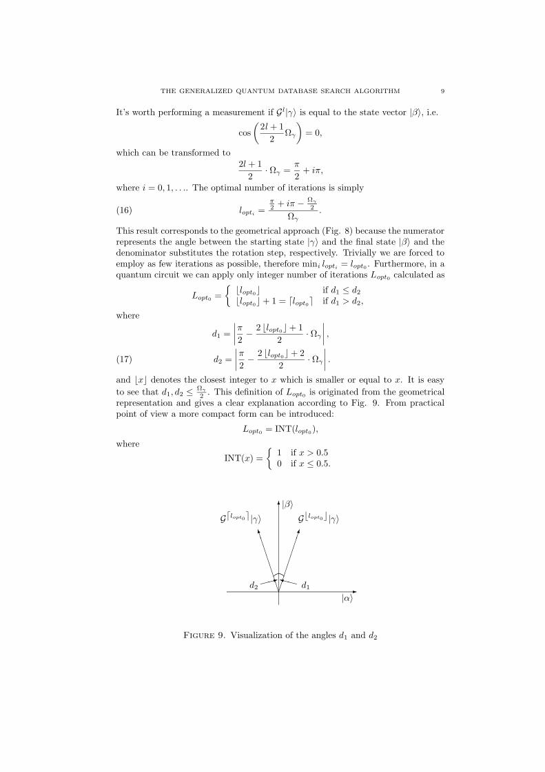
= lopt0 . Furthermore, in aquantum circuit we can apply only integer number of iterations Lopt0 calculated as

Lopt0 =

blopt0c if d1 ≤ d2

blopt0c + 1 = dlopt0e if d1 > d2,

where

d1 =

∣∣∣∣

π

2− 2 blopt0c + 1

2· Ωγ

∣∣∣∣,

d2 =

∣∣∣∣

π

2− 2 blopt0c + 2

2· Ωγ

∣∣∣∣.(17)

and bxc denotes the closest integer to x which is smaller or equal to x. It is easy

to see that d1, d2 ≤ Ωγ

2 . This definition of Lopt0 is originated from the geometricalrepresentation and gives a clear explanation according to Fig. 9. From practicalpoint of view a more compact form can be introduced:

Lopt0 = INT(lopt0),

where

INT(x) =

1 if x > 0.50 if x ≤ 0.5.

6

-

BB

BB

BBBM

|α〉

|β〉

d1d2:

Gdlopt0e|γ〉 Gblopt0c|γ〉

XXy

Figure 9. Visualization of the angles d1 and d2


In case of M N

(18) Ωγ ' sin Ωγ = 2

√

M

N,

yielding from (14), where the optimal number of evaluations is equal to

(19) Lopt0 ' π

4

√

M

N.

Now, we reached the surprising result Lopt0 = O(√

MN

)

. From (16) with i = 0 one

can easily spot the initial angle Ωγ/2 for a single query, which is Ωγ = 60. Thisleads to a special relation of size of the database N to the number of marked statesM (see Example 1.), which is

N = 4M.

2.3. Probability of Error. Rotating |γ〉 Lopt0 times with angle Ωγ , error mayoccur applying a measurement at the end of the database search, if |r〉 does notattain |β〉 exactly. It still remains a cosine scrap in (15), which is a projection ofGl|γ〉 on |α〉 describing the probability amplitude of the final state being in theunmarked basis vector state. Thus the probability of error resulting from basicGrover’s search algorithm is calculated as

(20) Pε = cos2(

(2Lopt0 + 1) Ωγ

2

)

,

and the Probability of Success

(21) Ps = 1 − Pε = sin2

((2Lopt0 + 1) Ωγ

2

)

.

Since d1, d2 ≤ Ωγ

2 therefore Pε ≤ sin2(

Ωγ

2

)

. Substituting Ωγ according to (18),

Pε ≤ MN

. Finally, we have an important remark. Equation (16) highlights the factthat we have a tradeoff between Pε and Lopti

, because lopt0 is only a local minimumplace of number of iterations. This inspire us to search for the global optimum infunction of i if the accuracy of the measurement is playing more important role thanthe number of Grover steps. Fortunately, the generalized Grover search algorithm isable to guarantee sure success measurement using about Lopt0 iterations. However,if we are restricted to buy the original Grover quantum search circuit at the grocer’sit is worth seeking for the global optimum.

3. Several Remarks on the Proportion of Marked States and the

Size of the Database

In previous subsections it was introduced a proportion√

M/N between thenumber of marked states M and the dimension of search space N , that makes asignificant contribution to the effectiveness of the search algorithm. The initialstate |γ〉 according to (14), the angle of rotation Ωγ as well as the required numberof iterations lopti

from (16), which include the speed and the performance Pε of thesearch in (20), are all depending from this ratio. The larger it is the less is Ωγ andlarger is l as depicted in Fig. 11 and 12. Consequently, finding a slight numberof marked entries in a huge database, the initial state may converge to |β〉 withhigher accuracy but at the cost of more iterations, keeping off the oscillation about


it, resulting in a lower Pε. However, one should keep in mind that the number ofiterations is still far lower as in classical searching algorithm even in these situations.

Let us examine several bounds for√

M/N .

• It is unambiguous that√

M/N must be less or equal one, since it wouldstand for more marked states than the entire number of entries in thedatabase.

• A trivial solution is when√

M/N is equal to one, which means an initial

angleΩγ

2 = π2 , which implies no needed rotation. Each measurement carries

out the proper solution, however, this case happens occasionally.• Let us determine the values for M

Nwhen it is worth performing the mea-

surement directly without any iteration, i.e. Lopt0= 0. According to (16)

and taking into account the property sin(x) = cos(

π2 − x

)and (14),

lopt0 =π2 − Ωγ

2

2Ωγ

2

=arccos

(√MN

)

2 arcsin(√

MN

) < 0.5,

or

arccos

(√

M

N

)

< arcsin

(√

M

N

)

.

Employing simple trigonometrical calculus (see Fig. 10) it turns out asolution

√2

2<

√

M

N≤ 1,

from which the bounds become

(22)1

2<M

N≤ 1.

Since, sin(

Ωγ

2

)

= MN

, therefore expression (22) is equivalent to π4 < Ωγ ≤ π

2

in terms of initial state angle. If Lopt0 = 0 we have two choices. Eitherwe perform measurement without any iteration. The probability of successis in this case Ps = M

N≥ 1

2 . Or we double the size of the database using

unmarked entries. Hence, MN

⇒ M2N

< 12 and we can increase the accuracy

(Ps) at the cost of more iteration steps. Clearly speaking the size of thedatabase does not need to be increased instead only one qubit should beadded to the index qregister and the Oracle should be programmed in thatway it answers f(x) = 0 for x > N !

As an example let M be chosen to 0.75 · 232, whereas the size of the databaseshould be 32 qubits long. The proportion M

N= 0.75.Following equations (16) and

(20), there is no need for anz rotation and at the same time Pε = 0.25. Adding asingle qubit to the index register N becomes 233, whereby M

N= 0.075. For a proper

solution one should apply the Grover’s search iteration twice to obtain an errorprobability Pε = 0.033, which is ∼ 86.6% better than previously at a cost of onlyfor 2 iterations. Finally observing Fig. 11 and 12 one can draw the conclusion thatin typical scenarios where M N the probability of error is dramatically reduced.


−1 −0.8 −0.6 −0.4 −0.2 0 0.2 0.4 0.7071 1−0.5

0

0.5

1

1.5

2

2.5

3

x

y

ArcSinArcCos

Figure 10. Intersection of arccos(x) and arcsin(x)

2 4 6 8 10 12 14 16 18 200

306090

120150

Ωγ

2 4 6 8 10 12 14 16 18 200

25

50

75

100

l

2 4 6 8 10 12 14 16 18 200

0.1

0.2

0.3

Pε

2 4 6 8 10 12 14 16 18 200.7

0.8

0.9

1

Size of the database −− # of qubits

Ps

Figure 11. Varying of the rotation angle Ωγ , the number of iter-ations l, the Probability of Error Pε and the Probability of Success(Ps) with increasing size of the database. M = 3, N = 2(2,...,19)

4. Generalized Grover Algorithm

During the analysis of the basic Grover algorithm we found that one should keepan eye on a contradictory fact, that the result of a search should be obtained usingas less iterations as possible meanwhile achieving high accuracy. For that reasona generalized Grover’s search algorithm is introduced and discussed in the nextsubsections.

4.1. Motivation. According to the utilization of Grover’s database search algo-rithm in practice, larger quantum systems should be taken into account where theinput index register of the algorithm is given as an arbitrary output state of a


2 5 10 15 20 25 300

153045607590

Ωγ

2 5 10 15 20 25 300

25

50

75

100

l

2 5 10 15 20 25 300

0.025

0.05

0.075

0.1

2 5 10 15 20 25 300.9

0.95

1

Ps

Size of the database −− # of qubits

Pε

Figure 12. Varying of the rotation angle Ωγ , the number of iter-ations l, the Probability of Error Pε and the Probability of Success(Ps) with increasing size of the database. M = 1, N = 2(2,...,30)

former circuit and the output of the algorithm can feed another circuit withoutany measurement. Hence the exact knowledge of the index register after the finaliteration is of great significance.

4.2. Generalization of the Original Grover’s Database Search Algorithm.

In order to give the generalization of the basic Grover algorithm we rewrite in thissubsection the original relations and introduce some new definitions, respectively.

In Section 2.1 the Grover operator was originally defined as

G , HPHO,

where

P , (2|0〉〈0| − I) ,

O , I − 2|y〉〈y|and

|γ〉 , H⊗n |0〉n =1√N

N−1∑

x=0

|x〉,

are determined as defined in (4), (5), where N = 2n denotes the number of itemsin the database, again.

Henceforth let us apply some new necessary definitions and practical considera-tions.

(1) From now onward H should be replaced by an arbitrary unitary transfor-mation U (H → U).


(2) The Oracle (O) should rotate the probability amplitude of the marked itemsin the index register with an angle of φ in lieu of π, set originally, whereφ ∈ [−π, π]. Thus (5) is altered to

(23) O → Iβ , I +(eφ − 1

)∑

x∈S

|y〉〈y|.

(3) Analogue to the Oracle above, the controlled phase gate (P) which wasoriginally based on the state |0〉 have to be founded on an arbitrary basisstate |η〉 resulting in a multiplication by eθ instead of −1, where θ ∈ [−π, π].In more exact mathematical formalism

(24) P → Iη , I +(eθ − 1

)|η〉〈η|.

(4) Furthermore the initial state of index register is considered as

(25) |γ〉 ,

2n−1∑

x=0

γx|x〉,

where∑(2n−1)

x=0 |γx|2 = 1 as appropriate.(5) Finally the two basis vectors |α〉 and |β〉 consisting of the indexes leading

to unmarked solutions and of the indexes ending in a marked entry shouldbe redefined, that were originally set in (11) and (12), respectively

|α〉 =1

√∑

x∈S |γx|2∑

x∈S

γx|x〉,(26)

|β〉 =1

√∑

x∈S |γx|2∑

x∈S

γx|x〉,(27)

where S represents the complementary set of indexes to S.

4.2.1. Properties of the Newly Defined Basis Vectors. We digress for a mo-ment to discuss the properties of newly defined basis vectors |α〉 and |β〉.

• Vector |α〉 is built from items x which do not lead to a solution andtherefore there do not lie in the set S, |α〉 =

∑

x∈S αx|x〉.• Observing the new basis vectors |α〉 and |β〉 the orthogonality is still

given between them, 〈α|β〉 = 0, since during the pairwise multiplica-tion within the inner product one of the factors is always zero.

• It is obvious that neither |α〉 nor |β〉 could be |0〉, except the extremeand unambiguous cases, when the search can not lead to a solution(since |β〉 = 0) and the case (|α〉 = 0) where a search would be sense-less since a measurement shows the result with a probability of one,immediately.

Regarding the definitions in (23) and (23) the generalized Grover operation (G → Q)looks like as follows

Q = −UIηU†Iβ = −U(I +

(eθ − 1

)|η〉〈η|

)U†Iβ

= −(UIU−1 +

(eθ − 1

)U|η〉〈η|U†) Iβ

Q = −(I +

(eθ − 1

)|µ〉〈µ|

)Iβ ,(28)

where

(29) |µ〉 , U|η〉


and relation U† = U−1 is exploited in consequence of the unitary operation property,respectively.

Before continuing our examinations, let us prove the completeness of the search.

Lemma 4.1. If the state vectors |α〉 and |β〉 are defined according to (26) and (27),as well as the unitary operator U and an arbitrary state |η〉 are taken in such a waythat U|η〉 lies within the vector space spanned by the state vectors |α〉 and |β〉, thenthe generalized Grover operator (Q) preserves this 2-dimensional vector space.For any |v〉 ∈ V , Q|v〉 ∈ V is true.

Proof. Following the geometrical definition of inner product, the length of the pro-jection of U|η〉 on vector |β〉 is 〈β|U|η〉 · |β〉. Since U|η〉 is defined in the vectorspace V , the vector U|η〉− 〈β|U|η〉|β〉 is parallel to |α〉 and it is exactly the ,,lengthof the vector” times |α〉,

U|η〉 − 〈β|U|η〉|β〉 =

√

1 − |〈β|U|η〉|β〉|2|α〉.Hence, |α〉 can be expressed as

|α〉 =1

√

1 − |〈β|U|η〉|2(U|η〉 − 〈β|U|η〉|β〉) .

Vector |µ〉 is considered as an arbitrary unit vector in V

(30) |µ〉2 = cos (Ω) |α〉 + sin (Ω) eΛ|β〉,where Ω,Λ ∈ [−π, π].

As the next step the generalized Grover operator should be given in V .

(31) Q|β〉 = −UIηU†Iβ |β〉,the required two dimensional Grover matrix and the basis vectors are searched inthe form of

Q2 =

[Q11 Q12

Q21 Q22

]

.

As Iβ multiplies every indexes leading to a marked entry by eφ,

(32) Iβ |β〉 = eφ|β〉.Equation (31) alters considering (32) to

Q|β〉 = −[UIU−1 +

(eθ − 1

)|µ〉〈µ|

]eφ|β〉

= −eφ|β〉(eθ − 1

)eφU|η〉〈η|U−1|β〉

= −eφ((eθ − 1

)〈µ|β〉|µ〉 + |β〉

).(33)

Applying (30) and the relation 〈µ|β〉 = 〈β|µ〉∗ = sin (Ω) e−Λ, where |µ〉 is accordingto (29),

Q|β〉 = −eφ(eθ − 1

)sin (Ω) e−Λ

(cos (Ω) |α〉 + sin (Ω) eΛ|β〉

)− eφ|β〉

= −eφ(eθ − 1

)sin (Ω) cos (Ω) e−Λ

︸︷︷︸

Q21

|α〉

+−eφ[(eθ − 1

)sin2 (Ω) + 1

]

︸︷︷︸

Q22

|β〉.(34)


Moreover, the further two entries in Q

Q|α〉 = −[I +

(eθ − 1

)|µ〉〈µ|Iβ |α〉

],(35)

where Iβ |α〉 = |α〉, because only the indexes leading to a solution are rotated byIβ otherwise will be maintained, which ends to

(36) 〈µ|α〉 = 〈α|µ〉∗ = cos (Ω) .

Thus, similar to (34)

Q|α〉 = −[1 +

(eθ − 1

)cos2 (Ω)

]

︸︷︷︸

Q11

|α〉

+ −[(eθ − 1

)cos (Ω) sin (Ω) eΛ

]

︸︷︷︸

Q12

|β〉(37)

Now, from (34) and (37) we conclude that Q|α〉 and Q|β〉 is remained in the vectorspace V , therefore all the linear superposition

|v〉 = a|α〉 + b|β〉,

of |α〉 and |β〉 transformed by Q still remained in the vector space V .

Based on equations (34) and (37) we have matrix Q2 in a suitable two dimen-sional form

Q2 = −

[1 +

(eθ − 1

)cos2 (Ω) eφ

(eθ − 1

)sin (Ω) cos (Ω) e−Λ

(eθ − 1

)cos (Ω) sin (Ω) eΛ eφ

[1 +

(eθ − 1

)sin2 (Ω)

]

]

= −

[

eθ cos2 (Ω) + sin2 (Ω) eφe−Λ(eθ − 1

) sin(2Ω)2(

eθ − 1)eΛ sin(2Ω)

2eφ[eθ sin2 (Ω) + cos2 (Ω)

]

]

.

(38)

From this point forward Q always refers to the two dimensional Grover matrix, ifotherwise not indicated.

4.3. Required Number of Iterations in the Generalized Grover’s Search

Algorithm. After being acquainted with the 2-dimensional generalized Groveroperator Q, the optimal number of iterations lopt during a search should be derived.Thus, we follow the assumption

〈α|Qlopt |γ〉 = 0,

which stands for having an index register orthogonal to the vector including all theindexes which do not lead to a solution. Because |α〉 and |β〉 are orthogonal, thisassumption can be interpreted as Qlopt |γ〉 is parallel to |β〉 i.e. Qlopt |γ〉 = eδ|β〉.In this case sure success can be reached after a measurement. Since Q is an unitaryoperator and therefore it is a normal operator, hence it has a spectral decomposition

(39) Q = q1|ψ1〉 + q2|ψ2〉,

where q1,2 denote the eigenvalues of Q and |ψ1,2〉 stand for the eigenvectors of Q,respectively, with the concatenation

(40) Q|ψ1,2〉 = q1,2|ψ1,2〉,


where 〈ψ1|ψ2〉 = 0, because of the orthogonality between the eigenvectors. Theeigenvalues determined from the characteristic equation det Q − qI = 0 (see Ap-pendix A) are

(41) q1,2 = −e( θ+φ2 ±∆).

In addition we claim the following restriction on the angle ∆

(42) cos∆ = cos

(θ − φ

2

)

+ sin2 (Ω)

(

cos

(θ + φ

2

)

− cos

(θ − φ

2

))

.

In possession of the eigenvalues the next step towards the optimal number ofiterations is the determination of the normalized eigenvectors |ψ1,2〉, which are

|ψ1〉 = cos (z) e(φ2 −Λ)|α〉 + sin (z) |β〉,(43)

|ψ2〉 = − sin (z) e(φ2 −Λ)|α〉 + cos (z) |β〉,(44)

where

sin2(z) =sin2 (2Ω) sin2

(θ2

)

2(

1 − cos(

θ2

)cos(

φ2 − ∆

)

− 2 cos (2Ω) sin(

θ2

)sin(

φ2 − ∆

)) .

The detailed derivation of the eigenvectors and eigenvalues can be found in theAppendix (A and B).

Due to the spectral decomposition and the relation 〈ψ1|ψ2〉 = 〈ψ2|ψ1〉 = 0,

Ql = ql1|ψ1〉〈ψ1| + ql

2|ψ2〉〈ψ2|= (−1)

le·l( θ+φ

2 ) ·

·[

e2( φ2−Λ) (el∆ cos2 (z) + e−l∆ sin2 (z)

) sin (l∆) sin (2z) e( φ

2−Λ)

sin (l∆) sin (2z) e−( φ2−Λ) el∆ sin2 (z) + e−l∆ cos2 (z)

]

.

(45)

Using (45), l can be derived by

(46) 〈α|Ql|γ〉 = 0,

which is fulfilled if both –the real and the imaginary– part of (46) are equal to zero.Let |γ〉 be defined as an arbitrary unit vector in V

|γ〉 = cos (Ωγ) |α〉 + sin (Ωγ) eΛγ |β〉.Thus,

〈α|Ql|γ〉 = cos (Ωγ)Ql11 + sin (Ωγ) eΛγQl

12 =

= cos (Ωγ)[el∆ cos2 (z) + e−l∆ sin2 (z)

]+

+ e(φ2 −Λ+Λγ) sin (l∆) sin (2z) sin (Ωγ) = 0(47)

The real part of (47) is

<〈α|Ql|γ〉

= cos (Ωγ)

[cos (l∆) cos2 (z) + cos (l∆) sin2 (z)

]

︸︷︷︸

cos(l∆)

−

− sin

(

Λγ − Λ +φ

2

)

sin (l∆) sin (2z) sin (Ωγ) =


(48) = cos (Ωγ) cos (l∆) − sin (Ωγ) sin (l∆) sin (2z) sin

(

Λγ − Λ +φ

2

)

= 0,

whereas the imaginary one is equal to

=〈α|Ql|γ〉

= cos (Ωγ)

[sin (l∆) cos2 (z) − sin (l∆) sin2 (z)

]

︸︷︷︸

sin(l∆) cos(2z)

+

+cos

(

Λγ − Λ +φ

2

)

sin (l∆) sin (2z) = 0.

Since, sin (l∆) 6= 0, the imaginary part becomes

=

〈α|Ql|γ〉

=

= cos

(

Λγ − Λ +φ

2

)

sin (2z) sin (Ωγ) + cos (Ωγ) cos (2z) = 0.(49)

4.3.1. Matching Condition. Equation (49) does not depend on l, which makes itappropriate to determine the so called ,,matching condition” (MC), the relationshipbetween θ and φ,

cos

(

Λγ − Λ +φ

2

)

= − cot (2z) cot (Ωγ) ,

and thus

(50) tan

(φ

2

)

=cos (2Ω) + sin (2Ω) · tan (Ωγ) cos (Λ − Λγ)

cot φ2 − tan (Ωγ) sin (2Ω) sin (Λ − Λγ)

.

It is worth emphasizing, that according to (42) ∆ is 4π periodical in function of θ,which includes clasping a 4π range of φ by determining φ form θ, since ∆ is alsodepends on φ. This seems to be in contradiction that the eigenvalues q1,2 shouldbe 2π periodical in θ and φ. This problem can be eliminated if φ is calculated forthe range [−2π, 2π] in function of θ ∈ [−2π, 2π]. Practically ±2π should be addedto φ if it has a cut-off in the function.

−2pi −pi 0 pi 2pi −2pi

−pi

0

pi

2pi

θ

φ

Figure 13. The angles φ vs. θ without and with correction

The points where φ (θ) has cut-off’s within the range of [−π, π] are the pointswhere

φ = ±π ⇒ tan

(φ

2

)

= ±∞.


Inasmuch as, the numerator of the matching condition in (50) is constant in θ, thedenominator have to be zero to achieve the condition φ = ±∞. The cut-off anglesθco1,2

can be derived from denominator of (50) as follows. From (50),

cot

(φ

2

)

= tan (Ωγ) sin (2Ω) sin (Λ − Λγ)

the cut-off angles in [−2π, 2π] are

θco1= 2arctan (tan (Ωγ) sin (2Ω) sin (Λ − Λγ)) ,(51)

θco2= θco1

± 2π.(52)

By means of this correction 2π periodicity of ∆ is achieved, hence, the eigenvaluesand eigenvectors of Q, even Q itself can boast a 2π periodicity in θ.

4.3.2. Optimal Number of Iterations. Now, the way is open to determine l from(49) which provides a measurement with Pε = 0. The matching condition (50)should be also considered leading to

cos

(

l∆ + arcsin

(

sin

(φ

2− Λ + Λγ

)

sin (Ωγ)

))

= 0,

which is equivalent to

(53) l∆ = ±π2± iπ − arcsin

(

sin

(φ

2− Λ + Λγ

)

sin (Ωγ)

)

,

where ±iπ is omitted from the right hand side, because it would result in a bigger l.Unlike the basic algorithm where i > 0 could result in a more accurate measurementin case of the generalized algorithm i = 0 provides Pε = 0, Expression (53) can beinterpreted in the following way. The generalized Grover operator (Q) rotates thenew initial state |γ〉′ with the initial angle Ωγ = arcsin

(sin(

φ

2− Λ + Λγ

)sin (Ωγ)

)in

a plane V ′ spanned by the basis vectors |α〉′ and |β〉′ with a single rotation angle∆ towards |β〉′ as it is depicted in Fig. 14. It shall be remarked that |α〉′ and |β〉′are real valued axes while |α〉 and |β〉 are complex valued.

6

-1

|α〉′

|β〉′

|γ〉′

Q|γ〉′

Ω′γ∆

Figure 14. Geometrical interpretation of the generalized Grover iteration


Because of the arbitrary sing of sin(

φ2 − Λ + Λγ

)

, Ω′γ can take different values,

depending on

(54) ν = arcsin

(

sin

(φ

2− Λ + Λγ

)

sin (Ωγ)

)

,

where arcsin(·) and arccos(·) are defined as

|arcsin (·)| ≤ π

2and

0 ≤ arccos (·) ≤ π.

If ν is positive the initial angle Ω′γ could be (π − ν) or (ν), in the other case the

possible values are (−π+ν) or (−π). According to the matching condition |∆| ≤ π2 ,

and because +|β〉 is as appropriate for final state as −|β〉 therefore ±|β〉 can bereached from Ω′

γ by means of an overall rotation smaller than π2 . The number of

iteration lMC can be expressed from (53) as

(55) lMC =

π2 −

∣∣∣arcsin

(

sin(

φ2 − Λ + Λγ

)

sin (Ωγ))∣∣∣

∆,

which leads to a sure success measurement.

0 pi 2pi0

1.54

5

10

θ

l

Figure 15. Number of iteration l assuming the matching con-dition is fulfilled, when the parameter setting was Ω = 0.5,Ωγ = 0.0001, Λγ = 0.005, Λ = 0.005

4.3.3. The Final State of the Index Register Before the Measurement. An importantcase could arise when the output of the Grover algorithm should be applied as aninput to another circuit. It could be helpful to know the final state of the indexregister without measuring it. If the initial state with a global phase factor isexpressed as

|γ〉 =[cos (Ωγ) |α〉 + sin (Ωγ) eΛγ |β〉

]· eδ,

after lMC iterations

QlMC |γ〉 = eδe(lMC(π+ φ+Θ2 +ε))|β〉,

where(−1)

lMC = eπ·lMC .


and

ε = arctan

(

cot

(φ

2− Λ + Λγ

))

.

4.3.4. Possible Variable Settings According to lMC . The required number of gener-alized Grover iteration lMC in (55) refined by the matching condition is typicallynot an integer. Hence, several cases are worthwhile to discuss how to employ thegeneralized Grover operator (Q) in order to provide sure success.

(A) In this case the variables |γ〉, |µ〉, φ and θ are predefined. Unfortunately,this fact does not guarantee sure success. A subtask of this assumption isif the settings are θ = φ = π and Λ = Λγ as well as Ω = Ωγ ⇒ |γ〉 = |µ〉,which leads to the original Grover operator, introduced in Section 2.1.

(B) In the second case let us suppose freely adjustable rotation angles φ and

θ. The optimal θopt is computable from ∂lMC

∂θ= ∂lMC

∂φ· dφ

dθ+ ∂lMC

∂θ= 0,

i.e. we determine the minimum point of lMC in Fig. 15, from which theoptimal rotation angle φopt can be derived applying the matching condition(50), and henceforth the optimal number of iterations lopt may be find outaccording to (55), respectively. Since l is not an integer for sure, the –to thenext nearest superior positive integer– rounded up Lopt1 should be takeninto account. In consequence of this deferral, the matching condition isharmed, which infer a calibration of the angle θ and φ. From Lopt1 we cancalculate φ′

opt1from (55) and substituting it into (50) we get θ′opt1

.(C) In our last case we strive for a single rotation step to the solution. For this

purpose only the initial state |γ〉, thus also Ωγ and Λγ is given antecedently,whereas all the other parameters are freely customizable.

Starting form equation (55), with LMC = 1

∆ =π

2− arcsin

(

sin

(φ

2− Λ + Λγ

)

sin (Ωγ)

)

.

In addition taking the cosine of both sides and substituting cos(∆) form(42) leads to

(56) tan

(φ

2

)

=sin (Ωγ) sin (Λγ − Λ) − cos

(θ2

)

sin(

θ2

)cos (2Ω) − cos (Λγ − Λ) sin (Ωγ)

after some trigonometrical calculus. In order to fulfil the matching condi-

tion expression (56) should be set equal to tan(

φ2

)

in (50) by tuning the

variables Ω, Λ and θ. This method corresponds to the following visualiza-tion: for a given initial state |γ〉 the reflection axis |µ〉 is tuned in the vector

space V in such a way that it leads to a single rotation to eδe(π+ φ+θ2 +ε),

resulting in a solution with a probability of one after a measurement. Itshould be emphasized that in the original Grover algorithm |µ〉 = |γ〉 isused.

5. Example

(1) In this example let us have a look at the possible setting of variables inthe generalized Grover’s search algorithm introduced in Section 4.3.4–C.We examine the algorithm by setting the variables Λ = Λγ and θ = φ =π resulting almost in the original Grover operator (G), except that the


reflection axis |µ〉 of the inversion about average operator differs from |γ〉.From equations (50) and (56)

cos (2Ω) + sin (2Ω) tan (Ωγ)

cot(

θ2

) =cos(

θ2

)

sin (Ωγ) − sin(

θ2

)cos (2Ω)

,

cos (2Ω) + sin (2Ω) tan (Ωγ) = 0,

resulting in

Ω =π2 − Ωγ

2,

which meets our requirement Lopt = 1.Finally we emphasize that the definition of Ωγ is different in case of basic

and the generalized Grover algorithm. In the former case Ωγ denotes thedouble of the angle between |γ〉 and |α〉. In the latter case Ωγ refers to theangle between |γ〉 and |α〉.

6. Conclusions

In this paper we introduced a new generalized Grover operator description ap-plied in quantum database search algorithm. We reviewed the basic Grover data-base search algorithm and introduced the general Grover operator. We also showedthat it is possible to perform a quantum database search using only a single iterationwith possibility of success equal one after a measurement.

References

[1] L.K. Grover, “A fast quantum mechanical algorithm for database search,” Proceedings, 28thAnnual ACM Symposium on the Theory of Computing, pp. 212–219, May 1996. quant-ph/9605043.

[2] L. K. Grover, “Quantum mechanics helps in searching for a needle in a haystack,” Phys. Rev.Lett., vol. 79, pp. 325–328, July 1997. e-print quant-ph/9706033.

[3] C. Zalka, “Grover’s quantum searching algorithm is optimal,” quant-ph/9711070v2, Decem-ber 1999.

[4] M. Boyer, G. Brassard, P. Hoyer, A. Tapp, “Tight bounds on quantum searching,” Proceed-

ings 4th Workshop on Physics and Computation, vol. 46, no. 4-5, pp. 36–43, 1996. Also inFortschritte der Physik, Vol. 46, No. 4-5, 1998, pp. 493-505 quant-ph/9605034.

[5] C. H. Bennett, E. Bernstein, G. Brassard, U. Vazirani, “Strengths and weakness of quantumcomputing,” SIAM Journal on Computing, vol. 26, no. 5, pp. 1510–1523, 1997. e-print quant-

ph/9701001.

[6] C. Zalka, “Simulating quantum systems on a quantum computer,” Phys. Rev. A., pp. 313–322, 1998.

[7] D. Aharonov, “Quantum computation,” Annual Reviews of Computational Physics, vol. VI.,1999. e-print http://www.cs.huji.ac.il/ doria/papers.html.

[8] L. K. Grover, “Quantum computers can search rapidly by using almost any transformation,”Phys. Rev. Lett, vol. 80, no. 19, pp. 4329–4332, 1998. e-print quant-ph/9712011.

[9] G. L. Long, Y. S. Li, W. L. Zang and L. Niu, “Phase matching in quantum searching,” Phys.

Lett., vol. A 262, no. 27, pp. 27–34, 1999. e-print quant-ph/9906020.[10] G. Brassard, P. Hoyer, M. Mosca, A. Tapp, “Quantum amplitude amplification and estima-

tion,” Quantum Computation & Quantum Information Science, AMS Contemporary MathSeries, e-print quant-ph/0005055.

[11] P. Hoyer, “Arbitrary phases in quantum amplitude amplification,” Phys. Lett., vol. A 62,

2000. e-print quant-ph/0006031.[12] G. L. Long, C. C. Tu, Y. S. Li, W. L. Zang and L. Niu, “A novel so(3) picture for quantum

searching,” Phys. Lett., 1999. e-print quant-ph/9911004.[13] G. L. Long, “Grover algorithm with zero theoretical failure rate,” 2001. e-print quant-

ph/0106071.


[14] G. L. Long, L. Xiao, Y. Sun, “General phase matching condition for quantum searching,”2001. e-print quant-ph/0107013.

[15] J-Y. Hsieh, C-M. Li, “A general su(2) formulation for quantum searching with certainity,”

2001. e-print quant-ph/0112035.

[16] D. Biron, O. Biham, E. Biham, M. Grassl, D.A. Lidar, Generalized Grover Search Algorithm

for Arbitrary Initial Amplitude Distribution. Lecture Notes in Computer Science, Springer,1998. Proceedings of the 1st NASA International Conference on Quantum Computing and

Quantum Communications, e-print quant-ph/9801066.

[17] E. Biham, O. Biham, D. Biron , M. Grassl, D.A. Lidar, Grover’s Search Algorithm for an

Arbitrary Initial Amplitude Distribution, vol. 1509 of Lecture Notes in Computer Science,

pp. 140–147. Springer, 1998. Quantum Computing & Quantum Communications; First NASA

International Conference; selected papers, QCQC’98, C.P. Williams (ed.), e-print quant-

ph/9807027.

[18] E. Biham, O. Biham, D. Biron , M. Grassl, D.A. Lidar, D. Shapira, “Analysis of generalized

grover’s search algoritms using recursion equations,” Phys. Rev., vol. A 63, no. 012310, 2001.

e-print quant-ph/00100077.

[19] G. Brassard, P. Hoyer, A. Tapp, Quantum Counting, vol. 1443 of Lecture Notes in Computer

Science, pp. 820–831. Springer, July 1998. Proceedings of the 25th International Colloquiumon Automata, Languages, and Programming, e-print quant-ph/9805082.

[20] C. Durr, P. Hoyer, “A quantum algorithm for finding the minimum,” 1996. e-print quant-

ph/9607014.[21] A. Ahuja, S. Kapoor, “A quantum algorithm for finding the maximum,” e-print quant-

ph/9911082.[22] S. Imre, F. Balazs, Quantum Multi-User Detection in” Application & Services in Wireless

Networks”, pp. 126–133. Innovative Technology Series, Hermes Penton Science, 2001. ISBN:1-9039-9630-9.

[23] S. Imre, F. Balazs, “Non-coherent multi-user detection based on quantum search,” IEEE

International Conference on Communication (ICC), 2002.[24] S. Imre, F. Balazs, “A tight bound for probability of error for quantum counting based mul-

tiuser detection,” IEEE International Symposium on Information Theory (ISIT’02), p. 43,

Juni 30- July 5 2002.[25] L. Grover, “Tradeoffs in the quantum search algorithm,” 2002. e-print quant-ph/0201152.

Appendix A. Eigenvalues of the generalized Grover operator (Q)

First, we give a detailed derivation of the eigenvalues of the generalized Grover’ssearch algorithm solving the characteristic function det Q − qI, which is a quiethard task.

(Q11 − q) (Q22 − q) −Q12Q21 = 0,

q1,2 =Q11 +Q22 ±

√

(Q11 +Q22)2 − 4 (Q11Q22 −Q12Q21)

2.(57)

With the assumption of the basis independent product of eigenvalues with the formof det Q = q1q2 as well as with the form of eigenvalues of unitary operators eε,

(58) det (Q) = Q11Q22 −Q12Q21,

Q11Q22 = (−1)(−1)[

1 +(

eθ − 1

)

cos2 (Ω)]

eφ[

1 +(

eθ − 1

)

sin2 (Ω)]

= eφ

1 +

(

eθ − 1

) (sin2 (Ω) + cos2 (Ω)

)

︸︷︷︸

≡1

+(

eθ − 1

)2

sin2 (Ω) cos2 (Ω)

= eφ

[(

eθ − 1

)2

sin2 (Ω) cos2 (Ω)

]

.(59)


Q12Q21 = (−1)(−1)eφ(

eθ − 1

)

sin (Ω) cos (Ω) eΛ(

eθ − 1

)

sin (Ω) cos (Ω) e−Λ =

= eφ[(

eθ − 1

)

sin2 (Ω) cos2 (Ω)]

.(60)

Substituting (59) and (60) in (58),

(61) det (Q) = e(θ+φ),

since qi = eεi , by which the eigenvalues of the generalized Grover operator are

(62) q1,2 = −e( θ+φ2 ±∆).

Furthermore, it is known that the trace of Q can be expressed as

(63) Q11 +Q22 = q1 + q2,

resulting in

Q11 +Q22 =

= −[

1 +(

eθ − 1

)

cos2 (Ω) + eφ(

eθ − 1

)

sin2 (Ω)]

= −

1 − cos2 (Ω)︸︷︷︸

sin2(Ω)

+eθ cos2 (Ω)︸︷︷︸

1−sin2(Ω)

+eφ+

+e(φ+θ) sin2 (Ω) − eφ sin2 (Ω)

]

=

= −[

sin2 (Ω) + eθ + e

φ − sin2 (Ω)(

−eθ − eφ + e

(φ+θ))]

,(64)

where the equality stands if both the real and the imaginary part of (64) holdsseparately. The imaginary one looks like

=Q11 +Q22 =

= −[sin (θ) + sin (φ) + sin2 (Ω) (− sin (θ) − sin (φ) + sin (φ+ θ))

]=

= −

2 sin

(φ+ θ

2

)

cos

(φ− θ

2

)

+

+ sin2 (Ω)

[

sin

(φ+ θ

2cos

(φ− θ

2

))

+ 2 sin

(φ+ θ

2

)]

,(65)

where the trigonometrical definition[sinx+ sin y = 2 sin

(x+y

2

)cos(

x+y2

)]is em-

ployed. Applying (62) on (63) and substituting into (64),

=q1 + q2 = −

sin

(θ + φ

2+ ∆

)

+ sin

(θ + φ

2− ∆

)

= −2 sin

(θ + φ

2

)

cos (∆) .(66)


From (65) and (66),

cos ∆ = cos

(φ− θ

2

)

+ sin2 (Ω)

(

cos

(θ + φ

2

)

− cos

(φ− θ

2

))

= cos

(φ− θ

2

)

− 2 sin2 (Ω) sin

(φ

2

)

sin

(θ

2

)

= cos

(φ

2

)

cos

(θ

2

)

+ sin

(φ

2

)

sin

(θ

2

)[1 − 2 sin2 (Ω)

]

= cos

(φ

2

)

cos

(θ

2

)

+ sin

(φ

2

)

sin

(θ

2

)

cos (2Ω) .(67)

The derivation of the real part of (64) is straightforward, hence,

<Q11 +Q22 =

−[

2 cos

(θ + φ

2

)

cos

(θ − φ

2

)

+ sin2 (Ω) · 2 cos2(θ + φ

2

)]

,(68)

thus

(69) <q1 + q2 = −2 cos

(θ + φ

2

)

cos (∆) ,

whereas we reached the same result as in (67)

cos∆ = cos

(θ − φ

2

)

+ sin2 (Ω)

(

cos

(θ + φ

2

)

− cos

(θ − φ

2

))

,

as it was shown in (42).Consequently, only one restriction is noticeable, namely on cos∆, which is

cos∆ = cos (−∆). At the same time according to the special form of the eigenval-ues in (62) the two ∆’s are equivalent to each other, since both lead to the sameeigenvalue pair.

Appendix B. Eigenvectors of the generalized Grover’s search

algorithm

In possession of knowledge about Q and the eigenvalues q1,2, derived above in(62), also the eigenvectors should be found out to the full description of the spectraldecomposition of Q.

Starting form (40) and the expression

(70) |ψ1〉 = ψ1α|α〉 + ψ1β |β〉,a homogenous linear equation system is obtained

Q11ψ1α +Q12ψ1β = q1ψ1α,

Q21ψ1α +Q22ψ1β = q2ψ1β ,(71)

from which

ψ1α

ψ1β

=q1 −Q22

Q21,(72)

ψ1β

ψ1α

=q1 −Q11

Q12.(73)


Apparently, there are infinite many solution of (71), which difference in a scalarfactor. For our purposes we only need those with a unit length in a form

(74) |ψ〉norm = cos(z)eC |α〉 + sin(z)|β〉.

According to (72) let ψ1α = q1 −Q22 and ψ1β = Q22. From the possible solutionswe focus our attention on those, which has unit length, ‖|ψ1〉norm‖ = 1, thus,∣∣cos(z)eC

∣∣2

+ |sin(z)|2 = 1, where

sin2(z) =|ψ1β |2

|ψ1α|2 + |ψ1β |2,(75)

cos2(z) =|ψ1α|2

|ψ1α|2 + |ψ1β |2.(76)

Following our antecedent establishments

|ψ1α|2 = |q1 −Q22|2 =

=

<()︷︸︸︷(

− cos

(θ + φ

2+ ∆

)

+ sin2(Ω) cos

(θ + φ

2

)

+ cos2(Ω) cos(φ)

)2

+

+

(

− sin

(θ + φ

2+ ∆

)

+ sin2(Ω) sin

(θ + φ

2

)

+ cos2(Ω) sin(φ)

)2

︸︷︷︸

=()

,

(77)

and

(78) |ψ1α|2 = ψ1αψ∗1α,

(79) |ψ1β |2 = ψ1βψ∗1β ,


respectively. As the next step let us derive |ψ1α/ψ1β |2 as follows∣∣∣∣

ψ1α

ψ1β

∣∣∣∣

2

=−e( θ+φ

2+∆) + eφ

[(eθ − 1

)sin2 (Ω) + 1

]

−eφ (eθ − 1) sin (Ω) cos (Ω) e−Λ·

·−e−( θ+φ

2+∆) + e−φ

[(e−θ − 1

)sin2 (Ω) + 1

]

−e−φ (e−θ − 1) sin (Ω) cos (Ω) eΛ

=

(

1 − e( θ−φ2

+∆) +(eθ − 1

)sin2 (Ω)

)

(eθ − 1) (e−θ − 1) sin2 (Ω) cos2 (Ω)·

·

(

1 − e−( θ−φ2

+∆) +(e−θ − 1

)sin2 (Ω)

)

(eθ − 1) (e−θ − 1) sin2 (Ω) cos2 (Ω)

=

[

1 − e( θ−φ2

+∆) − e−( θ−φ2

+∆) + 1]

+[1 − e−θ − eθ + 1

]sin4 (Ω)

sin2 (Ω) cos2 (Ω) [1 − e−θ − eθ + 1]+

+sin2 (Ω)

[

eθ − 1 − e( θ+φ2

−∆) + e−( θ−φ2

+∆) + e−θ − 1 − e−( θ+φ2

−∆) + e( θ−φ2

+∆)]

sin2 (Ω) cos2 (Ω) [1 − e−θ − eθ + 1]=

=2 − 2 cos

(θ−φ

2+ ∆

)− sin2 (Ω) cos2 (Ω) [2 − 2 cos (θ)]

sin2 (Ω) cos2 (Ω) [2 − 2 cos (θ)]+

+sin2 (Ω)

[2 − 2 cos (θ) − 2 + 2 cos (θ) − 2 cos

(θ+φ

2− ∆

)+ 2 cos

(θ−φ

2+ ∆

)]

sin2 (Ω) cos2 (Ω) [2 − 2 cos (θ)]=

=2 − 2 cos

(θ−φ

2+ ∆

)−

sin2(2Ω)︷︸︸︷

sin2 (Ω) cos2 (Ω) 4 sin2(

θ2

)

sin2 (2Ω) sin2(

θ2

) +

+sin2 (Ω)

[2 cos

(θ−φ

2+ ∆

)− 2 cos

(θ+φ

2− ∆

)]

sin2 (2Ω) sin2(

θ2

)(80)

Keeping in mind the expression (75), in which |ψ1α/ψ1β |2 is given in (80),

|ψ1β |2

|ψ1α|2 + |ψ1β |2=

sin2 (2Ω) sin2(

θ2

)

2 − 2 cos(

θ−φ

2+ ∆

)sin2 (Ω)

[2 cos

(θ−φ

2+ ∆

)− 2 cos

(θ+φ

2− ∆

)]

=sin2 (2Ω) sin2

(θ2

)

2 − 2 cos(

θ−φ

2+ ∆

)+ 4 sin2 (Ω) sin

(θ2

)sin(

φ

2− ∆

)

=sin2 (2Ω) sin2

(θ2

)

2 − 2 cos(

θ2

)cos(

φ

2− ∆

)− 2 sin

(θ

2

)

sin

(φ

2− ∆

)

+ 4 sin2 (Ω) sin

(θ

2

)

sin

(φ

2− ∆

)

︸︷︷︸

sin( θ2 ) sin( φ

2−∆)

(4 sin2 (Ω) − 2

)

︸︷︷︸

−2 cos(2Ω)

sin2(z) =sin2 (2Ω) sin2

(θ2

)

2(1 − cos

(θ2

)cos(

φ

2− ∆

)− 2 cos (2Ω) sin

(θ2

)sin(

φ

2− ∆

)) .(81)

(82) cos2(z) = 1 − sin2(z).

Finally, to determine the eigenvectors |ψ1,2〉, only eC part is remaining in (74).Considering the relation

ψ1α

ψ1β

=cos (z)

sin (z)eC1 ,


and thus ∣∣∣∣

ψ1α

ψ1β

∣∣∣∣

2

= cot2(z)e2C1 =Q12

Q21· q1 −Q22

q1 −Q11,

where equations (72), (73) were employed, and

cot(2z) =cos2 (z) − sin2 (z)

2√

sin2 (z) cos2 (z)=

|ψ1α|2 − |ψ1β |2

2√

|ψ1α|2 |ψ1β |2,

respectively. It can be proved that

q1 −Q22

q1 −Q11

is a real number, which implies that

(eC1

)2=Q12

Q21=e−Λeφ

e−Λ= e(φ−2Λ),

from which follows

(83) eC1 = ±e(φ2 −Λ).

Based on (83) the normalized eigenvector

(84) |ψ1〉 = cos (z) e(φ2 −Λ)|α〉 + sin (z) |β〉.

Eigenvector |ψ2〉 have to be calculated in a similar way, where the other eigenvalueq2 should be taken into account, which results in a simple sign change of ∆. Due tothe definition of C2 in (74), it does not depend on the sign of ∆, thus eC2 = ±eC1 .To become the eigenvectors |ψ1〉 and |ψ2〉 orthogonal, eC2 must be equal to −eC1 ,whereas the second eigenvector will be

(85) |ψ2〉 = − sin (z) e(φ2 −Λ)|α〉 + cos (z) |β〉.

Budapest University of Technology and Economics, Department of Telecommuni-

cation, Mobile Communications and Computing Laboratory, H-1117 Budapest, Magyar

tudosok korutja 2., HUNGARY

E-mail address: [email protected]

Documents

THE GENERALIZED QUANTUM DATABASE SEARCH