Embed Size (px)
DESCRIPTION
This book describes some basic ideas in set theory, model theory, proof theory, and recursion theory; these are all parts of what is called mathematical logic.
Citation preview
The Foundations of Mathematics
c©2005,2006,2007 Kenneth Kunen
Kenneth Kunen
October 29, 2007

Contents
0 Introduction 30.1 Prerequisites . . . . . . . . . . . . . . . . . . . . . . . . . . . . . . . . . . 30.2 Logical Notation . . . . . . . . . . . . . . . . . . . . . . . . . . . . . . . 30.3 Why Read This Book? . . . . . . . . . . . . . . . . . . . . . . . . . . . . 50.4 The Foundations of Mathematics . . . . . . . . . . . . . . . . . . . . . . 5
I Set Theory 10I.1 Plan . . . . . . . . . . . . . . . . . . . . . . . . . . . . . . . . . . . . . . 10I.2 The Axioms . . . . . . . . . . . . . . . . . . . . . . . . . . . . . . . . . . 10I.3 Two Remarks on Presentation. . . . . . . . . . . . . . . . . . . . . . . . 14I.4 Set theory is the theory of everything . . . . . . . . . . . . . . . . . . . . 14I.5 Counting . . . . . . . . . . . . . . . . . . . . . . . . . . . . . . . . . . . . 15I.6 Extensionality, Comprehension, Pairing, Union . . . . . . . . . . . . . . . 17I.7 Relations, Functions, Discrete Mathematics . . . . . . . . . . . . . . . . . 24
I.7.1 Basics . . . . . . . . . . . . . . . . . . . . . . . . . . . . . . . . . 24I.7.2 Foundational Remarks . . . . . . . . . . . . . . . . . . . . . . . . 29I.7.3 Well-orderings . . . . . . . . . . . . . . . . . . . . . . . . . . . . . 31
I.8 Ordinals . . . . . . . . . . . . . . . . . . . . . . . . . . . . . . . . . . . . 33I.9 Induction and Recursion on the Ordinals . . . . . . . . . . . . . . . . . . 42I.10 Power Sets . . . . . . . . . . . . . . . . . . . . . . . . . . . . . . . . . . . 46I.11 Cardinals . . . . . . . . . . . . . . . . . . . . . . . . . . . . . . . . . . . 48I.12 The Axiom of Choice (AC) . . . . . . . . . . . . . . . . . . . . . . . . . . 56I.13 Cardinal Arithmetic . . . . . . . . . . . . . . . . . . . . . . . . . . . . . 61I.14 The Axiom of Foundation . . . . . . . . . . . . . . . . . . . . . . . . . . 66I.15 Real Numbers and Symbolic Entities . . . . . . . . . . . . . . . . . . . . 73
II Model Theory and Proof Theory 78II.1 Plan . . . . . . . . . . . . . . . . . . . . . . . . . . . . . . . . . . . . . . 78II.2 Historical Introduction to Proof Theory . . . . . . . . . . . . . . . . . . . 78II.3 NON-Historical Introduction to Model Theory . . . . . . . . . . . . . . . 80II.4 Polish Notation . . . . . . . . . . . . . . . . . . . . . . . . . . . . . . . . 81II.5 First-Order Logic Syntax . . . . . . . . . . . . . . . . . . . . . . . . . . . 85
1

CONTENTS 2
II.6 Abbreviations . . . . . . . . . . . . . . . . . . . . . . . . . . . . . . . . . 91II.7 First-Order Logic Semantics . . . . . . . . . . . . . . . . . . . . . . . . . 92II.8 Further Semantic Notions . . . . . . . . . . . . . . . . . . . . . . . . . . 98II.9 Tautologies . . . . . . . . . . . . . . . . . . . . . . . . . . . . . . . . . . 105II.10 Formal Proofs . . . . . . . . . . . . . . . . . . . . . . . . . . . . . . . . . 106II.11 Some Strategies for Constructing Proofs . . . . . . . . . . . . . . . . . . 110II.12 The Completeness Theorem . . . . . . . . . . . . . . . . . . . . . . . . . 116II.13 More Model Theory . . . . . . . . . . . . . . . . . . . . . . . . . . . . . . 127II.14 Equational Varieties and Horn Theories . . . . . . . . . . . . . . . . . . . 132II.15 Extensions by Definitions . . . . . . . . . . . . . . . . . . . . . . . . . . . 135II.16 Elementary Submodels . . . . . . . . . . . . . . . . . . . . . . . . . . . . 138II.17 Other Proof Theories . . . . . . . . . . . . . . . . . . . . . . . . . . . . . 142
IIIRecursion Theory 143
Bibliography 144

Chapter 0
Introduction
0.1 Prerequisites
It is assumed that the reader knows basic undergraduate mathematics. Specifically:You should feel comfortable thinking about abstract mathematical structures such
as groups and fields. You should also know the basics of calculus, including some of thetheory behind the basics, such as the meaning of limit and the fact that the set R of realnumbers is uncountable, while the set Q of rational numbers is countable.
You should also know the basics of logic, as is used in elementary mathematics.This includes truth tables for boolean expressions, and the use of predicate logic inmathematics as an abbreviation for more verbose English statements.
0.2 Logical Notation
Ordinary mathematical exposition uses an informal mixture of English words and logicalnotation. There is nothing “deep” about such notation; it is just a convenient abbrevia-tion which sometimes increases clarity (and sometimes doesn’t). In Chapter II, we shallstudy logical notation in a formal way, but even before we get there, we shall use logicalnotation frequently, so we comment on it here.
For example, when talking about the real numbers, we might say
∀x[x2 > 4→ [x > 2 ∨ x < −2]] ,
or we might say in English, that for all x, if x2 > 4 then either x > 2 or x < −2.Our logical notation uses the propositional connectives ∨,∧,¬,→,↔ to abbreviate,
respectively, the English “or”, “and”, “not”, “implies”, and “iff” (if and only if). It alsouses the quantifiers, ∀x and ∃x to abbreviate the English “for all x” and “there existsx”.
Note that when using a quantifier, one must always have in mind some intendeddomain of discourse, or universe over which the variables are ranging. Thus, in the
3

CHAPTER 0. INTRODUCTION 4
above example, whether we use the symbolic “∀x” or we say in English, “for all x”, itis understood that we mean for all real numbers x. It also presumes that the variousfunctions (e.g. x 7→ x2) and relations (e.g, <) mentioned have some understood meaningon this intended domain, and that the various objects mentioned (4 and ±2) are in thedomain.
“∃!y” is shorthand for “there is a unique y”. For example, again using the realnumbers as our universe, it is true that
∀x[x > 0→ ∃!y[y2 = x ∧ y > 0]] ; (∗)
that is, every positive number has a unique positive square root. If instead we used therational numbers as our universe, then statement (∗) would be false.
The “∃!” could be avoided, since ∃!y ϕ(y) is equvalent to the longer expression∃y [ϕ(y) ∧ ∀z[ϕ(z) → z = y]], but since uniqueness statements are so common in math-ematics, it is useful to have some shorthand for them.
Statement (∗) is a sentence, meaning that it has no free variables. Thus, if theuniverse is given, then (∗) must be either true or false. The fragment ∃!y[y2 = x∧ y > 0]is a formula, and makes an assertion about the free variable x; in a given universe, itmay be true of some values of x and false of others; for example, in R, it is true of 3 andfalse of −3.
Mathematical exposition will often omit quantifiers, and leave it to the reader to fillthem in. For example, when we say that the commutative law, x · y = y · x, holds inR, we are really asserting the sentence ∀x, y[x · y = y · x]. When we say “the equationax + b = 0 can always be solved in R (assuming a 6= 0)”, we are really asserting that
∀a, b[a 6= 0→ ∃x[a · x + b = 0]] .
We know to use a ∀a, b but an ∃x because “a, b” come from the front of the alphabetand “x” from near the end. Since this book emphasizes logic, we shall try to be moreexplicit about the use of quantifiers.
We state here for reference the usual truth tables for ∨,∧,¬,→,↔:
Table 1: Truth Tables
ϕ ψ ϕ ∨ ψ ϕ ∧ ψ ϕ→ ψ ϕ↔ ψT T T T T TT F T F F FF T T F T FF F F F T T
ϕ ¬ϕT FF T
Note that in mathematics, ϕ → ψ is always equivalent to ¬ϕ ∨ ψ. For example,7 < 8 → 1 + 1 = 2 and 8 < 7 → 1 + 1 = 2 are both true; despite the English rendering
CHAPTER 0. INTRODUCTION 5
of “implies”, there is no “causal connection” between 7 < 8 and the value of 1 + 1. Also,note that “or” in mathematics is always inclusive; that is ϕ ∨ ψ is true if one or both ofϕ, ψ are true, unlike the informal English in “Stop or I’ll shoot!”.
0.3 Why Read This Book?
This book describes some basic ideas in set theory, model theory, proof theory, andrecursion theory; these are all parts of what is called mathematical logic. There arethree reasons one might want to read about this:
1. As an introduction to logic.
2. For its applications in topology, analysis, algebra, AI, databases.
3. Because the foundations of mathematics is relevant to philosophy.
1. If you plan to become a logician, then you will need this material to understandmore advanced work in the subject.
2. Set theory is useful in any area of math dealing with uncountable sets; modeltheory is closely related to algebra. Questions about decidability come up frequently inmath and computer science. Also, areas in computer science such as artificial intelligenceand databases often use notions from model theory and proof theory.
3. The title of this book is “Foundations of Mathematics”, and there are a numberof philosophical questions about this subject. Whether or not you are interested in thephilosophy, it is a good way to tie together the various topics, so we’ll begin with that.
0.4 The Foundations of Mathematics
The foundations of mathematics involves the axiomatic method. This means that inmathematics, one writes down axioms and proves theorems from the axioms. The justi-fication for the axioms (why they are interesting, or true in some sense, or worth studying)is part of the motivation, or physics, or philosophy, not part of the mathematics. Themathematics itself consists of logical deductions from the axioms.
Here are three examples of the axiomatic method. The first two should be knownfrom high school or college mathematics.
Example 1: Geometry. The use of geometry (in measurement, construction, etc.)is prehistoric, and probably evolved independently in various cultures. The axiomaticdevelopment was first (as far as we know) developed by the ancient Greeks from 500 to300 BC, and was described in detail by Euclid around 300 BC. In his Elements [12], helisted axioms and derived theorems from the axioms. We shall not list all the axioms ofgeometry, because they are complicated and not related to the subject of this book. Onesuch axiom (see Book I, Postulate 1) is that any two distinct points determine a unique
CHAPTER 0. INTRODUCTION 6
line. Of course, Euclid said this in Greek, not in English, but we could also say it usinglogical notation, as in Section 0.2:
∀x, y [[Point(x) ∧ Point(y) ∧ x 6= y]→ ∃!z[Line(z) ∧ LiesOn(x, z) ∧ LiesOn(y, z)]] .
The intended domain of discourse, or universe, could be all geometric objects.
Example 2: Group Theory. The group idea, as applied to permutations and alge-braic equations, dates from around 1800 (Ruffini 1799, Abel 1824, Galois 1832). Theaxiomatic treatment is usually attributed to Cayley (1854) (see [4], Vol 8). We shall listall the group axioms because they are simple and will provide a useful example for us aswe go on. A group is a model (G; ·) for the axioms GP = {γ1, γ2}:
γ1. ∀xyz[x · (y · z) = (x · y) · z]γ2. ∃u[∀x[x · u = u · x = x] ∧ ∀x∃y[x · y = y · x = u]]
Here, we’re saying that G is a set and · is a function from G × G into G such that γ1
and γ2 hold in G (with “∀x” meaning “for all x ∈ G”, so G is our universe, as discussedin Section 0.2). Axiom γ1 is the associative law. Axiom γ2 says that there is an identityelement u, and that for every x, there is an inverse y, such that xy = yx = u. A moreformal discussion of models and axioms will occur in Chapter II.
From the axioms, one proves theorems. For example, the group axioms imply thecancellation rule. We say: GP ⊢ ∀xyz[x · y = x · z → y = z]. This turnstile symbol “⊢”is read “proves”.
This formal presentation is definitely not a direct quote from Cayley, who stated hisaxioms in English. Rather, it is influenced by the mathematical logic and set theory ofthe 1900s. Prior to that, axioms were stated in a natural language (e.g., Greek, English,etc.), and proofs were just given in “ordinary reasoning”; exactly what a proof is was notformally analyzed. This is still the case now in most of mathematics. Logical symbolsare frequently used as abbreviations of English words, but most math books assume thatyou can recognize a correct proof when you see it, without formal analysis. However,the Foundations of Mathematics should give a precise definition of what a mathematicalstatement is and what a mathematical proof is, as we do in Chapter II, which coversmodel theory and proof theory.
This formal analysis makes a clear distinction between syntax and semantics. GP isviewed as a set of two sentences in predicate logic; this is a formal language with preciserules of formation (just like computer languages such as C or java or TEX or html). Aformal proof is then a finite sequence of sentences in this formal language obeying someprecisely defined rules of inference – for example, the Modus Ponens rule (see SectionII.10) says that from ϕ→ ψ and ϕ you can infer ψ. So, the sentences of predicate logicand the formal proofs are syntactic objects. Once we have given a precise definition,it will not be hard to show (see Exercise II.11.11) that there really is a formal proof ofcancellation from the axioms GP

CHAPTER 0. INTRODUCTION 7
Semantics involves meaning, or structures, such as groups. The syntax and semanticsare related by the Completeness Theorem (see Theorem II.12.1), which says that GP ⊢ ϕiff ϕ is true in all groups.
After the Completeness Theorem, model theory and proof theory diverge. Prooftheory studies more deeply the structure of formal proofs, whereas model theory empha-sizes primarily the semantics – that is, the mathematical structure of the models. Forexample, let G be an infinite group. Then G has a subgroup H ⊆ G which is countablyinfinite. Also, given any cardinal number κ ≥ |G|, there is a group K ⊇ G of size κ.Proving these statements is an easy algebra exercises if you know some set theory, whichyou will after reading Chapter I.
These statements are part of model theory, not group theory, because they are spe-cial cases of the Lowenheim–Skolem-Tarski Theorem (see Theorems II.16.4 and II.16.5),which applies to models of arbitrary theories. You can also get H,K to satisfy all thefirst-order properties true in G. For example if G is non-abelian, then H,K will be also.Likewise for other properties, such as “abelian” or “3-divisible” (∀x∃y(yyy = x)). Theproof, along with the definition of “first-order”, is part of model theory (Chapter II),but the proof uses facts about cardinal numbers from set theory, which brings us to thethird example:
Example 3: Set Theory. For infinite sets, the basic work was done by Cantor inthe 1880s and 1890s, although the idea of sets — especially finite ones, occurred muchearlier. This is our first topic, so you will soon see a lot about uncountable cardinalnumbers. Cantor just worked naively, not axiomatically, although he was aware thatnaive reasoning could lead to contradictions. The first axiomatic approach was due toZermelo (1908), and was improved later by Fraenkel and von Neumann, leading to thecurrent system ZFC (see Section I.2), which is now considered to be the “standard”axioms for set theory.
A philosophical remark: In model theory, every list of sentences in formal logic formsthe axioms for some (maybe uninteresting) axiomatic theory, but informally, there aretwo different uses to the word “axioms”: as “statements of faith” and as “definitionalaxioms”. The first use is closest to the dictionary definition of an axiom as a “truism”or a “statement that needs no proof because its truth is obvious”. The second use iscommon in algebra, where one speaks of the “axioms” for groups, rings, fields, etc.
Consider our three examples:Example 1 (Classical Greek view): these are statements of faith — that is, they are
obviously true facts about real physical space, from which one may then derive othertrue but non-obvious facts, so that by studying Euclidean geometry, one is studyingthe structure of the real world. The intended universe is fixed – it could be thoughtof as all geometric objects in the physical universe. Of course, Plato pointed out that“perfect” lines, triangles, etc. only exist in some abstract idealization of the universe,but no one doubted that the results of Euclidean geometry could be safely applied tosolve real-world problems.

CHAPTER 0. INTRODUCTION 8
Example 2 (Everyone’s view): these are definitional axioms. The axioms do notcapture any deep “universal truth”; they only serve to define a useful class of structure.Groups occur naturally in many areas of mathematics, so one might as well encapsulatetheir properties and prove theorems about them. Group theory is the study of groups ingeneral, not one specific group, and the intended domain of discourse is the particulargroup under discussion.
This view of Example 2 has never changed since the subject was first studied, butour view of geometry has evolved. First of all, as Einstein pointed out, the Euclideanaxioms are false in real physical space, and will yield incorrect results when applied toreal-world problems. Furthemore, most modern uses of geometry are not axiomatic. Wedefine 3-dimensional space as R3, and we discuss various metrics (notions of distance) onit, including the Euclidean metric, which approximately (but not exactly) corresponds toreality. Thus, in the modern view, geometry is the study of geometries, not one specificgeometry, and the Euclidean axioms have been downgraded to mere definitional axioms— one way of describing a specific (flat) geometry.
Example 3 (Classical (mid 1900s) view): these are statements of faith. ZFC is thetheory of everything (see Section I.4). Modern mathematics might seem to be a messof various axiom systems: groups, rings, fields, geometries, vector spaces, etc., etc. Thisis all subsumed within set theory, as we’ll see in Chapter I. So, we postulate once andfor all these ZFC axioms. Then, from these axioms, there are no further assumptions;we just make definitions and prove theorems. Working in ZFC , we say that a group isa set G together with a product on it satisfying γ1, γ2. The product operation is reallya function of two variables defined on G, but a function is also a special kind of set —namely, a set of ordered pairs. If you want to study geometry, you would want to knowthat a metric space is a set X, together with some distance function d on it satisfyingsome well-known properties. The distances, d(x, y), are real numbers. The real numbersform the specific set R, constructed within ZFC by a set-theoretic procedure which weshall describe later (see Definition I.15.4).
We study set theory first because it is the foundation of everything. Also, the dis-cussion will produce some technical results on infinite cardinalities which are useful ina number of the more abstract areas of mathematics. In particular, these results areneeded for the model theory in Chapter II; they are also important in analysis andtopology and algebra, as you will see from various exercises in this book. In Chapter I,we shall state the axioms precisely, but the proofs will be informal, as they are in mostmath texts. When we get to Chapter II, we shall look at formal proofs from variousaxiom systems, and GP and ZFC will be interesting specific examples.
The ZFC axioms are listed in Section I.2. The list is rather long, but by the end ofChapter I, you should understand the meaning of each axiom and why it is important.Chapter I will also make some brief remarks on the interrelationships between the ax-ioms; further details on this are covered in texts in set theory, such as [18, 20]. Theseinterrelationships are not so simple, since ZFC does not settle everything of interest.Most notably, ZFC doesn’t determine the truth of the Continuum Hypotheses, CH .

CHAPTER 0. INTRODUCTION 9
This is the assertion that every uncountable subset of R has the same size as R.Example 3 (Modern view): these are definitional axioms. Set theory is the study of
models of ZFC . There are, for example, models in which 2ℵ0 = ℵ5; this means that thereare exactly four infinite cardinalities, called ℵ1,ℵ2,ℵ3,ℵ4, strictly between countable andthe size of R. By the end of Chapter I, you will understand exactly what CH and ℵnmean, but the models will only be hinted at.
Chapter III covers recursion theory, or the theory of algorithms and computability.Since most people have used a computer, the informal notion of algorithm is well-knownto the general public. The following sets are clearly decidable, in that you can writea program which tests for them in your favorite programming language (assuming thislanguage is something reasonable, like C or java or python):
1. The set of primes.
2. The set of axioms of ZFC .
3. The set of valid C programs.
That is, if you are not concerned with efficiency, you can easily write a program whichinputs a number or symbolic expression and tells you whether or not it’s a member ofone of these sets. For (1), you input an integer x > 1 and check to see if it is divisibleby any of the integers y with x > y > 1. For (2), you input a finite symbolic expressionand see if it is among the axiom types listed in Section I.2. Task (3) is somewhat harder,and you would have to refer to the C manual for the precise definition of the language,but a C compiler accomplishes task (3), among many other things.
Deeper results involve proving that certain sets which are not decidable, such as thefollowing:
4. The set of C programs which halt (say, with all values of their input).
5. {ϕ : ZFC ⊢ ϕ}.That is, there is no program which reads a sentences ϕ in the language of set theory andtells you whether or not ZFC ⊢ ϕ. Informally, “mathematical truth is not decidable”.Certainly, results of this form are relevant to the foundations of mathematics. Chapter IIIwill also be an introduction to understanding the meaning of some more advanced resultsalong this line, which are not proved in this book. Such results are relevant to many areasof mathematics. For example, {ϕ : GP ⊢ ϕ} is not decidable, whereas {ϕ : AGP ⊢ ϕ}is decidable, where AGP is the axioms for abelian groups. The proofs involve a lot ofgroup theory. Likewise, the solvability of diophantine equations (algebraic equations overZ) is undecidable; this proof involves a lot of number theory. Also, in topology, simpleconnectivity is undecidable. That is, there’s no algorithm which inputs a polyhedron(presented, for example, as a finite simplicial complex) and tells you whether or not it’ssimply connected. This proof involves some elementary facts about the fundamentalgroup in topology, plus the knowledge that the word problem for groups is undecidable.
This book only touches on the basics of recursion theory, but we shall give a precisedefinition of “decidable” and explain its relevance to set theory and model theory.

Chapter I
Set Theory
I.1 Plan
We shall discuss the axioms, explain their meaning in English, and show that from theseaxioms, you can derive all of mathematics. Of course, this chapter does not contain allof mathematics. Rather, it shows how you can develop, from the axioms of set theory,basic concepts, such as the concept of number and function and cardinality. Once thisis done, the rest of mathematics proceeds as it does in standard mathematics texts.
In addition to basic concepts, we describe how to compute with infinite cardinalities,such as ℵ0,ℵ1,ℵ2, . . . .
I.2 The Axioms
For reference, we list the axioms right off, although they will not all make sense untilthe end of this chapter. We work in predicate logic with binary relations = and ∈.
Informally, our universe is the class of all hereditary sets x; that is, x is a set, allelements of x are sets, all elements of elements of x are sets, and so forth. In this(Zermelo-Fraenkel style) formulation of the axioms, proper classes (such as our domainof discourse) do not exist. Further comments on the intended domain of discourse willbe made in Sections I.6 and I.14.
Formally, of course, we are just exhibiting a list of sentences in predicate logic.Axioms stated with free variables are understood to be universally quantified.
Axiom 0. Set Existence.∃x(x = x)
Axiom 1. Extensionality.
∀z(z ∈ x↔ z ∈ y) → x = y
10

CHAPTER I. SET THEORY 11
Axiom 2. Foundation.
∃y(y ∈ x) → ∃y(y ∈ x ∧ ¬∃z(z ∈ x ∧ z ∈ y))
Axiom 3. Comprehension Scheme. For each formula, ϕ, without y free,
∃y∀x(x ∈ y ↔ x ∈ z ∧ ϕ(x))
Axiom 4. Pairing.∃z(x ∈ z ∧ y ∈ z)
Axiom 5. Union.
∃A∀Y ∀x(x ∈ Y ∧ Y ∈ F → x ∈ A)
Axiom 6. Replacement Scheme. For each formula, ϕ, without B free,
∀x ∈ A ∃!y ϕ(x, y) → ∃B ∀x ∈ A ∃y ∈ B ϕ(x, y)
The rest of the axioms are a little easier to state using some defined notions. Onthe basis of Axioms 1,3,4,5, define ⊆ (subset), ∅ (or 0; empty set), S (ordinal successorfunction ), ∩ (intersection), and SING(x) (x is a singleton) by:
x ⊆ y ⇐⇒ ∀z(z ∈ x→ z ∈ y)
x = ∅ ⇐⇒ ∀z(z /∈ x)
y = S(x) ⇐⇒ ∀z(z ∈ y ↔ z ∈ x ∨ z = x)
w = x ∩ y ⇐⇒ ∀z(z ∈ w ↔ z ∈ x ∧ z ∈ y)
SING(x) ⇐⇒ ∃y ∈ x∀z ∈ x(z = y)
Axiom 7. Infinity.∃x
(∅ ∈ x ∧ ∀y ∈ x(S(y) ∈ x)
)
Axiom 8. Power Set.∃y∀z(z ⊆ x→ z ∈ y)
Axiom 9. Choice.
∅ /∈ F ∧ ∀x ∈ F ∀y ∈ F (x 6= y → x ∩ y = ∅) → ∃C ∀x ∈ F (SING(C ∩ x))
☛ ZFC = Axioms 1–9. ZF = Axioms 1–8.
☛ ZC and Z are ZFC and ZF , respectively, with Axiom 6 (Replacement) deleted.
☛ Z −, ZF−, ZC−,ZFC− are Z , ZF , ZC , ZFC , respectively, with Axiom 2 (Founda-tion) deleted.
CHAPTER I. SET THEORY 12
Most of elementary mathematics takes place within ZC − (approximately, Zermelo’stheory). The Replacement Axiom allows you to build sets of size ℵω and bigger. It alsolets you represent well-orderings by von Neumann ordinals, which is notationally useful,although not strictly necessary.
Foundation says that ∈ is well-founded – that is, every non-empty set x has an ∈-minimal element y. This rules out, e.g., sets a, b such that a ∈ b ∈ a. Foundation isnever needed in the development of mathematics.
Logical formulas with defined notions are viewed as abbreviations (or macros) forformulas in ∈,= only. In the case of defined predicates, such as ⊆, the macro is expandedby replacing the predicate by its definition (changing the names of variables as necessary),so that the Power Set Axiom abbreviates:
∀x∃y∀z((∀v(v ∈ z → v ∈ x))→ z ∈ y) .
In the case of defined functions, one must introduce additional quantifiers; the Axiom ofInfinity above abbreviates
∃x(∃u(∀v(v /∈ u) ∧ u ∈ x) ∧ ∀y ∈ x∃u(∀z(z ∈ u↔ z ∈ y ∨ z = y) ∧ u ∈ x)
).
Here, we have replaced the “S(y) ∈ x” by “∃u(ψ(y, u) ∧ u ∈ x)”, where ψ says that usatisfying the property of being equal to S(y).
We follow the usual convention in modern algebra and logic that basic facts about =are logical facts, and need not be stated when axiomatizing a theory. So, for example, theconverse to Extensionality, x = y → ∀z(z ∈ x ↔ z ∈ y), is true by logic – equivalently,true of all binary relations, not just ∈. Likewise, when we wrote down the axioms forgroups in Section 0.4, we just listed the axioms γ1, γ2 which are specific to the productfunction. We did not list statements such as ∀xyz(x = y → x · z = y · z); this is a factabout = which is true of any binary function.
In most treatments of formal logic (see Chapter II; especially Remark II.8.16), thestatement that the universe is non-empty (i.e., ∃x(x = x)) is also taken to be a logicalfact, but we have listed this explicitly as Axiom 0 to avoid possible confusion, since manymathematical definitions do allow empty structures (e.g., the empty topological space).
It is possible to ignore the “intended” interpretation of the axioms and just viewthem as making assertions about a binary relation on some non-empty domain. Thispoint of view is useful in seeing whether one axiom implies another. For example, #2 ofthe following exercise shows that Axiom 2 does not follow from Axioms 1,4,5.
Exercise I.2.1 Which of Axioms 1,2,4,5 are true of the binary relation E on the domainD, in the following examples?
1. D = {a};E = ∅.2. D = {a};E = {(a, a)}.

CHAPTER I. SET THEORY 13
3. D = {a, b};E = {(a, b), (b, a)}.4. D = {a, b, c};E = {(a, b), (b, a), (a, c), (b, c)}.5. D = {a, b, c};E = {(a, b), (a, c)}.6. D = {0, 1, 2, 3};E = {(0, 1), (0, 2), (0, 3), (1, 2), (1, 3), (2, 3)}.7. D = {a, b, c};E = {(a, b), (b, c)}.
a a a b a b
c
a b
c
0 1 2 3
a
b
c
Hint. It is often useful to picture E as a digraph (directed graph). The children ofa node y are the nodes x such that there is an arrow from x to y. For example, thechildren of node c in #4 are a and b. Then some of the axioms may be checked visually.Extensionality says that you never have two distinct nodes, x, y, with exactly the samechildren (as one has with b and c in #5). Pairing says that give any nodes x, y (possiblythe same), there is a node z with arrows from x and y into z. One can see at sight thatthis is true in #2 and false in the rest of the examples. �
Throughout this chapter, we shall often find it useful to think of membership as adigraph, where the children of a set are the members of the set. The simple finite modelspresented in Exercise I.2.1 are primarily curiosities, but general method of models (nowusing infinite ones) is behind all independence proofs in set theory; for example, there

CHAPTER I. SET THEORY 14
are models of all of ZFC in which the Continuum Hypothesis (CH ) is true, and othermodels in which CH is false; see [18, 20].
I.3 Two Remarks on Presentation.
Remark I.3.1 In discussing any axiomatic development — of set theory, of geometry,or whatever — be careful to distinguish between the:
• Formal discussion: definitions, theorems, proofs.
• Informal discussion: motivation, pictures, philosophy.
The informal discussion helps you understand the theorems and proofs, but is not strictlynecessary, and is not part of the mathematics. In most mathematics texts, including thisone, the informal discussion and the proving of theorems are interleaved. In this text,the formal discussion starts in the middle of Section I.6.
Remark I.3.2 Since we’re discussing foundations, the presentation of set theory will bea bit different than the presentation in most texts. In a beginning book on group theoryor calculus, it’s usually assumed that you know nothing at all about the subject, so youstart from the basics and work your way up through the middle-level results, and then tothe most advanced material at the end. However, since set theory is fundamental to allof mathematics, you already know all the middle-level material; for example, you knowthat R is infinite and {7, 8, 9} is a finite set of size 3. The focus will thus be on the reallybasic material and the advanced material. The basic material involves discussing themeaning of the axioms, and explaining, on the basis of the axioms, what exactly are 3and R. The advanced material includes properties of uncountable sets; for example, thefact that R, the plane R× R, and countably infinite dimensional space RN all have thesame size. When doing the basics, we shall use examples from the middle-level materialfor motivation. For example, one can illustrate properties of functions by using the real-valued functions you learn about in calculus. These illustrations should be consideredpart of the informal discussion of Remark I.3.1. Once you see how to derive elementarycalculus from the axioms, these illustrations could then be re-interpreted as part of theformal discussion.
I.4 Set theory is the theory of everything
First, as part of the motivation, we begin by explaining why set theory is the foundationof mathematics. Presumably, you know that set theory is important. You may not knowthat set theory is all -important. That is
• All abstract mathematical concepts are set-theoretic.
• All concrete mathematical objects are specific sets.

CHAPTER I. SET THEORY 15
Abstract concepts all reduce to set theory. For example, consider the notion offunction. Informally, a function gives you a specific way of corresponding y’s to x’s (e.g.,the function y = x2 + 1), but to make a precise definition of “function”, we identify afunction with its graph. That is, f is a function iff f is a set, all of whose elements areordered pairs, such that ∀x, y, z[(x, y) ∈ f ∧ (x, z) ∈ f → y = z]. This is a precisedefinition if you know what an ordered pair is.
Informally, (x, y) is a “thing” uniquely associated with x and y. Formally, we define(x, y) = {{x}, {x, y}}. In the axiomatic approach, you have to verify that the axioms letyou construct such a set, and that ZFC ⊢ “unique” , that is (see Exercise I.6.14):
ZFC ⊢ ∀x, y, x′, y′[(x, y) = (x′, y′)→ x = x′ ∧ y = y′] .
Then, a group is a special kind of pair (G, ·) where · is a function from G × G into G.G×G is the set of all ordered pairs from G. So, we explain everything in terms of sets,pairs, and functions, but it all reduces to sets. We shall see this in more detail later, aswe develop the axioms.
An example of concrete object is a specific number, like: 0, 1, 2,−2/3, π, e2i. Infor-mally, 2 denotes the concept of twoness – containing a thing and another thing andthat’s all. We could define two(x) ↔ ∃y, z[x = {y, z} ∧ y 6= z], but we want the officialobject 2 to be a specific set, not a logical formula. Formally, we pick a specific set withtwo distinct things in it and call that 2. Following von Neumann, let 2 = {0, 1}. Ofcourse, you need to know that 0 is a specific set with zero elements – i.e. 0 = ∅ and1 = {0} = {∅} ( a specific set with one element), which makes 2 = {∅, {∅}}. You cannow verify two(2).
The set of all natural numbers is denoted by N = ω = {0, 1, 2, 3, . . .}. Of course,3 = {0, 1, 2}. Once you have ω, it is straightforward to define the sets Z,Q,R,C. Theconstruction of Z,Q,R,C will be outlined briefly in Section I.15, with the details left toanalysis texts. You probably already know that Q is countable, while R and C are not.
I.5 Counting
Basic to understanding set theory is learning how to count. To count a set D of ducks,
you first have to get your ducks in a row, and then you pair them off against the naturalnumbers until you run out of ducks:

CHAPTER I. SET THEORY 16
0 1 2 3
Here we’ve paired them off with the elements of the natural number 4 = {0, 1, 2, 3}, sothere are 4 ducks : we say |D| = 4.
To count the set Q of rational numbers, you will have to use all of N = ω, since Qisn’t finite; the following picture indicates one of the standard ways for pairing Q offagainst the natural numbers:
0 1/1 −1/1 1/2 −1/2 2/1 −2/1 1/3 · · · · · ·0 1 2 3 4 5 6 7 · · · · · ·
we say |Q| = ω = ℵ0, the first infinite cardinal number. In our listing of Q: for each n,we make sure we have listed all rationals you can write with 0, 1, . . . , n, and we then goon to list the ones you can write with 0, 1, . . . , n, n+ 1.
Now, the set R of real numbers is uncountable; this only means that when you countit, you must go beyond the numbers you learned about in elementary school. Cantorshowed that if we take any list of ω real numbers, Lω = {a0, a1, a2, . . .} ⊆ R, thenthere will always be reals left over. But, there’s nothing stopping you from choosinga real in R\Lω and calling it aω, so you now have Lω+1 = {a0, a1, a2, . . . , aω} ⊆ R.You will still have reals left over, but you can now choose aω+1 ∈ R \ Lω+1, formingLω+2 = {a0, a1, a2, . . . , aω, aω+1}. You continue to count, using the ordinals:
0 , 1 , 2 , 3 , . . . , ω , ω + 1 , ω + 2 , . . . ω + ω , . . . , ω1 , . . .
In general Lα = {aξ : ξ < α}. If this isn’t all of R, you choose aα ∈ R \ Lα. Keep doingthis until you’ve listed all of R.
In the transfinite sequence of ordinals, each ordinal is the set of ordinals to the leftof it. We have already seen that 3 = {0, 1, 2} and ω is the set of natural numbers (orfinite ordinals). ω + ω is an example of a countable ordinal; that is, we can pair off itsmembers (i.e., the ordinals to the left of it) against the natural numbers:
0 ω 1 ω + 1 2 ω + 2 3 ω + 3 · · · · · ·0 1 2 3 4 5 6 7 · · · · · ·
If you keep going in these ordinals, you will eventually hit ω1 = ℵ1, the first uncountableordinal. If you use enough of these, you can count R or any other set. The ContinuumHypothesis , CH , asserts that you can count R using only the countable ordinals. CH isneither provable nor refutable from the axioms of ZFC .
We shall formalize ordinals and this iterated choosing later; see Sections I.8 and I.12.First, let’s discuss the axioms and what they mean and how to derive simple things (suchas the existence of the number 3) from them.
CHAPTER I. SET THEORY 17
I.6 Extensionality, Comprehension, Pairing, Union
We begin by discussing these four axioms and deriving some elementary results fromthem.
Axiom 1. Extensionality:
∀x, y [∀z(z ∈ x↔ z ∈ y) → x = y] .
As it says in Section I.2, all free variables are implicitly quantified universally. Thismeans that although the axiom is listed as just ∀z(z ∈ x↔ z ∈ y)→ x = y, the intentis to assert this statement for all x, y.
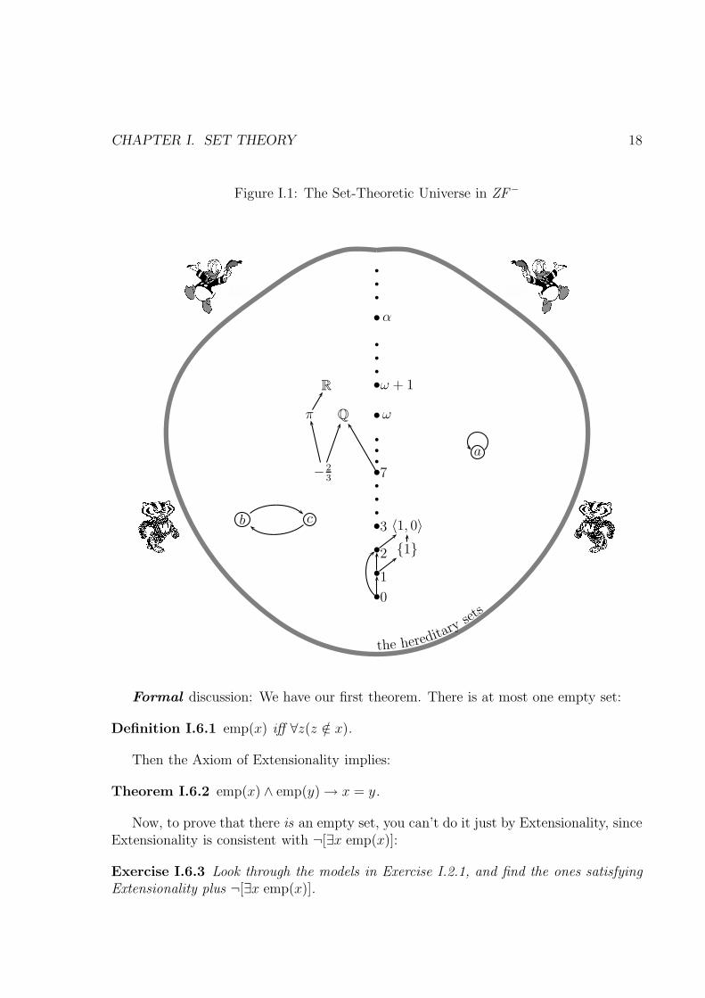
Informal discussion: This says that a set is determined by its members, so that ifx, y are two sets with exactly the same members, then x, y are the same set. Extension-ality also says something about our intended domain of discourse, or universe, which isusually called V (see Figure I.1, page 18). Everything in our universe must be a set,since if we allowed objects x, y which aren’t sets, such as a duck (D) and a badger (B),then they would have no members, so that we would have
∀z[z ∈ B ↔ z ∈ D ↔ z ∈ ∅ ↔ FALSE] ,
whereas B,D, ∅ are all different objects. So, physical objects, such as B,D, are not partof our universe.
Now, informally, one often thinks of sets or collections of physical objects, such as{B,D}, or a set of ducks (see Section I.5), or the set of animals in a zoo. However, thesesets are also not in our mathematical universe. Recall (see Section 0.2) that in writinglogical expressions, it is understood that the variables range only over our universe, sothat a statement such as “∀z · · · · · · ” is an abbreviation for “for all z in our universe· · · · · · ”. So, if we allowed {B} and {D} into our universe, then ∀z(z ∈ {B} ↔ z ∈ {D})would be true (since B,D are not in our universe), whereas {B} 6= {D}.
More generally, if x, y are (sets) in our universe, then all their elements are also inour universe, so that the hypothesis “∀z(z ∈ x↔ z ∈ y)” really means that x, y are setswith exactly the same members, so that Extensionality is justified in concluding thatx = y. So, if x is in our universe, then x must not only be a set, but all elements ofx, all elements of elements of x, etc. must be sets. We say that x is hereditarily a set(if we think of the members of x as the children of x, as in Exercise I.2.1, then we aresaying that x and all its descendents are sets). Examples of such hereditary sets are thenumbers 0, 1, 2, 3 discussed earlier.
So, the quantified variables in the axioms of set theory are intended to range over thestuff inside the blob in Figure I.1 — the hereditary sets. The arrows denote membership(∈). Not all arrows are shown. Extensionality doesn’t exclude sets a, b, c such thata = {a} and c ∈ b ∈ c. These sets are excluded by the Foundation Axiom (see SectionI.14), which implies that the universe is neatly arrayed in levels, with all arrows slopingup. Figure I.1 gives a picture of the universe under ZF−, which is set theory withoutthe Foundation Axiom.
CHAPTER I. SET THEORY 18
Figure I.1: The Set-Theoretic Universe in ZF−
b
b
b
b
b
b
b
b
0
1
2
3
7
ω
ω + 1
α
b
b
b
b
b
b
b
b
b
b
b
b
−23
π Q
R
{1}〈1, 0〉
a
b c
the hereditaryset
s
Formal discussion: We have our first theorem. There is at most one empty set:
Definition I.6.1 emp(x) iff ∀z(z /∈ x).
Then the Axiom of Extensionality implies:
Theorem I.6.2 emp(x) ∧ emp(y)→ x = y.
Now, to prove that there is an empty set, you can’t do it just by Extensionality, sinceExtensionality is consistent with ¬[∃x emp(x)]:
Exercise I.6.3 Look through the models in Exercise I.2.1, and find the ones satisfyingExtensionality plus ¬[∃x emp(x)].

CHAPTER I. SET THEORY 19
The usual proof that there is an empty set uses the Comprehension Axiom. As afirst approximation, we may postulate:
Garbage I.6.4 The Naive Comprehension Axiom (NCA) is the assertion: For everyproperty Q(x) of sets, the set S = {x : Q(x)} exists.
In particular, Q(x) can be something like x 6= x, which is always false, so that S willbe empty.
Unfortunately, there are two problems with NCA:
1. It’s vague.
2. It’s inconsistent.
Regarding Problem 2: Cantor knew that his set theory was inconsistent, and thatyou could get into trouble with sets which are too big. His contradiction (see SectionI.11) was a bit technical, and uses the notion of cardinality, which we haven’t discussedyet. However, Russell (1901) pointed out that one could rephrase Cantor’s paradox toget a really simple contradiction, directly from NCA alone:
Paradox I.6.5 (Russell) Applying NCA, define R = {x : x /∈ x}. Then R ∈ R↔ R /∈R, a contradiction.
Cantor’s advice was to avoid inconsistent sets (see [10]). This avoidance was in-corporated into Zermelo’s statement of the Comprehension Axiom as it is in SectionI.2. Namely, once you have a set z, you can form {x ∈ z : Q(x)}. You can still formR = Rz = {x ∈ z : x /∈ x}, but this only implies that if R ∈ z, then R ∈ R ↔ R /∈ R,which means that R /∈ z – that is,
Theorem I.6.6 There is no universal set: ∀z∃R[R /∈ z].
So, although we talk informally about the universe, V , it’s not really an object ofstudy in our universe of set theory.
Regarding Problem 1: What is a property? Say we have constructed ω, the set ofnatural numbers. In mathematics, we should not expect to form {n ∈ ω : n is stupid}.On a slightly more sophisticated level, so-called “paradoxes” arise from allowing ill-formed definitions. A well-known one is:
Let n be the least number which cannot be defined using fortywords of less. But I’ve just defined n in forty words of less.
Here, Q(x) says that x can be defined in 40 English words or less, and we try to form E ={n ∈ ω : Q(n)}, which is finite, since there are only finitely many possible definitions.Then the least n /∈ E is contradictory.
To avoid Problem 1, we say that a property is something defined by a logical formula,as described in Section 0.2 — that is, an expression made up using ∈, =, propositional

CHAPTER I. SET THEORY 20
(boolean) connectives (and, or, not, etc.), and variables and quantifiers ∀, ∃. So, ourprinciple now becomes: For each logical formula ϕ, we assert:
∀z[∃y∀x(x ∈ y ↔ x ∈ z ∧ ϕ(x))] .
Note that our proof of Theorem I.6.6 was correct, with ϕ(x) the formula x /∈ x. With adifferent ϕ, we get an empty set:
Definition I.6.7 ∅ denotes the (unique) y such that emp(y) (i.e., ∀x[x /∈ y]).
Justification. To prove that ∃y[emp(y)], start with any set z (there is one by Axiom0) and apply Comprehension with ϕ(x) a statement which is always false (for example,x 6= x) to get a y such that ∀x(x ∈ y ↔ FALSE) — i.e., ∀x(x /∈ y). By Theorem I.6.2,there is at most one empty set, so ∃!y emp(y), so we can name this unique object ∅. �
As usual in mathematics, before giving a name to an object satisfying some property(e.g.,
√2 is the unique y > 0 such that y2 = 2), we must prove that that property really
is held by a unique object.In applying Comprehension (along with other axioms), it is often a bit awkward to
refer back to the statement of the axiom, as we did in justifying Definition I.6.7. It willbe simpler to introduce some notation:
Notation I.6.8 For any formula ϕ(x):
☞ If there is a set A such that ∀x[x ∈ A↔ ϕ(x)], then A is unique by Extensionality,and we denote this set by {x : ϕ(x)}, and we say that {x : ϕ(x)} exists.
☞ If there is no such set, then we say that {x : ϕ(x)} doesn’t exist, or forms a properclass.
☞ {x ∈ z : ϕ(x)} abbreviates {x : x ∈ z ∧ ϕ(x)}.
Comprehension asserts that sets of the form {x : x ∈ z ∧ ϕ(x)} always exist. Wehave just seen that the empty set, ∅ = {x : x 6= x}, does exist, whereas a universal set,{x : x = x}, doesn’t exist. It’s sometimes convenient to “think” about this collectionand give it the name V , called the universal class, which is then a proper class. Weshall say more about proper classes later, when we have some more useful examples (seeNotation I.8.4). For now, just remember that the assertion “{x : x = x} doesn’t exist” issimply another way of saying that ¬∃A∀x[x ∈ A]. This is just a notational convention;there is no philosophical problem here, such as “how can we talk about it if it doesn’texist?”. Likewise, there is no logical problem with asserting “Trolls don’t exist”, andthere is no problem with thinking about trolls, whether or not you believe in them.
Three further remarks on Comprehension:1. Some elementary use of logic is needed even to state the axioms, since we need
the notion of “formula”. However, we’re not using logic yet for formal proofs. Once theaxioms are stated, the proofs in this chapter will be informal, as in most of mathematics.

CHAPTER I. SET THEORY 21
2. The Comprehension Axiom is really infinite scheme; we have one assertion foreach logical formula ϕ.
3. The terminology ϕ(x) just emphasizes the dependence of ϕ on x, but ϕ can haveother free variables, for example, when we define intersection and set difference:
Definition I.6.9 Given z, u:
☞ z ∩ u := {x ∈ z : x ∈ u}.☞ z \ u := {x ∈ z : x /∈ u}.
Here, ϕ is, respectively, x ∈ u and x /∈ u. For z ∩ u, the actual instance of Compre-hension used is: ∀u∀z∃y∀x(x ∈ y ↔ x ∈ z∧x ∈ u). To form z∪u, which can be biggerthan z and u, we need another axiom, the Union Axiom, discussed below.
Exercise I.6.10 Look through the models in Exercise I.2.1, and find one which satisfiesExtensionality and Comprehension but doesn’t have pairwise unions — that is, the modelwill contain elements z, u with no w satisfying ∀x[x ∈ w ↔ x ∈ z ∨ x ∈ u].
You have certainly seen ∪ and ∩ before, along with their basic properties; our em-phasis is how to derive what you already know from the axioms. So, for example, youknow that z ∩ u = u ∩ z; this is easily proved from the definition of ∩ (which impliesthat ∀x[x ∈ z ∩ u↔ x ∈ u ∩ z]) plus the Axiom of Extensionality. Likewise, z ∩ u ⊆ z;this is easily proved from the definition of ∩ and ⊆ :
Definition I.6.11 y ⊆ z ⇐⇒ ∀x(x ∈ y → x ∈ z).
In Comprehension, ϕ can even have z free – for example, it’s legitimate to formz∗ = {x ∈ z : ∃u(x ∈ u ∧ u ∈ z)}; so once we have officially defined 2 as {0, 1}, we’llhave 2∗ = {0, 1}∗ = {0}.
The proviso in Section I.2 that ϕ cannot have y free avoids self-referential definitionssuch as the Liar Paradox “This statement is false”: — that is
∃y∀x(x ∈ y ↔ x ∈ z ∧ x /∈ y)] .
is contradictory if z is any non-empty set.Note that ∅ is the only set whose existence we have actually demonstrated, and
Extensionality and Comprehension alone do not let us prove the existence of any non-empty set:
Exercise I.6.12 Look through the models in Exercise I.2.1, and find one which satisfiesExtensionality and Comprehension plus ∀x¬∃y[y ∈ x].

CHAPTER I. SET THEORY 22
We can construct non-empty sets using Pairing:
∀x, y ∃z (x ∈ z ∧ y ∈ z) .
As stated, z could contain other elements as well, but given z, we can always formu = {w ∈ z : w = x∨w = y}. So, u is the (unique by Extensionality) set which containsx, y and nothing else. This justifies the following definition of unordered and orderedpairs:
Definition I.6.13
☛ {x, y} = {w : w = x ∨ w = y}.☛ {x} = {x, x}.☛ 〈x, y〉 = (x, y) = {{x}, {x, y}}.The key fact about ordered pairs is:
Exercise I.6.14〈x, y〉 = 〈x′, y′〉 → x = x′ ∧ y = y′ .
Hint. Split into cases: x = y and x 6= y. �
There are many other definitions of ordered pair which satisfy this exercise. In mostof mathematics, it does not matter which definition was used – it is only important thatx and y are determined uniquely from their ordered pair; in these cases, it is conventionalto use the notation (x, y). We shall use 〈x, y〉 when it is relevant that we are using thisspecific definition.
We can now begin to count:
Definition I.6.15
0 = ∅1 = {0} = {∅}2 = {0, 1} = {∅, {∅}}
Exercise I.6.16 〈0, 1〉 = {1, 2}, and 〈1, 0〉 = {{1}, 2}.The axioms so far let us generate infinitely many different sets: ∅, {∅}, {{∅}}, . . . but
we can’t get any with more than two elements. To do that we use the Union Axiom.That will let us form 3 = 2 ∪ {2} = {0, 1, 2}. One could postulate an axiom which saysthat x∪ y exists for all x, y, but looking ahead, the usual statement of the Union Axiomwill justify infinite unions as well:
∀F ∃A ∀Y ∀x [x ∈ Y ∧ Y ∈ F → x ∈ A] .
That is, for any F (in our universe), view F as a family of sets. This axiom gives us aset A which contains all the members of members of F . We can now take the union ofthe sets in this family:

CHAPTER I. SET THEORY 23
Definition I.6.17 ⋃F =
⋃
Y ∈F
Y = {x : ∃Y ∈ F(x ∈ Y )}
That is, the members of⋃F are the members of members of F . As usual when writing
{x : · · · · · · }, we must justify the existence of this set.
Justification. Let A be as in the Union Axiom, and apply Comprehension to formB = {x ∈ A : ∃Y ∈ F(x ∈ Y )}. Then x ∈ B ↔ ∃Y ∈ F(x ∈ Y ). �
Definition I.6.18 u ∪ v =⋃{u, v}, {x, y, z} = {x, y} ∪ {z}, and {x, y, z, t} = {x, y} ∪
{z, t}.
You already know the basic facts about these notions, and, in line with Remark I.3.2,we shall not actually write out proofs of all these facts from the axioms. As two samples:
Exercise I.6.19 Prove that {x, y, z} = {x, z, y} and u ∩ (v ∪ w) = (u ∩ v) ∪ (u ∩ w).
These can easily be derived from the definitions, using Extensionality. For the secondone, note that an informal proof using a Venn diagram can beviewed as a shorthand for a rigorous proof by cases. For example,to prove that x ∈ u ∩ (v ∪ w) ↔ x ∈ (u ∩ v) ∪ (u ∩ w) for all x,you can consider the eight possible cases: x ∈ u, x ∈ v, x ∈ w,x ∈ u, x ∈ v, x /∈ w, x ∈ u, x /∈ v, x ∈ w, etc. In each case, youverify that the left and right sides of the “↔” are either both trueor both false. To summarize this longwinded proof in a picture,
v w
u
draw the standard Venn diagram of three sets, which breaks the plane into eight regions,and note that if you shade u∩ (v ∪w) or if you shade (u∩ v)∪ (u∩w) you get the samepicture. The shaded set consists of the regions for which the left and right sides of the“↔” are both true.
We can also define the intersection of a family of sets; as with pairwise intersection,this is justified directly from the Comprehension Axiom and requires no additional axiom:
Definition I.6.20 When F 6= ∅,⋂F =
⋂
Y ∈F
Y = {x : ∀Y ∈ F(x ∈ Y )}
Justification. Fix E ∈ F , and form {x ∈ E : ∀Y ∈ F(x ∈ Y )}. �
Note that⋃ ∅ = ∅, while
⋂ ∅ would be the universal class, V , which doesn’t exist.
We can now count a little further:

CHAPTER I. SET THEORY 24
Definition I.6.21 The ordinal successor function, S(x), is x ∪ {x}. Then define:
3 = S(2) = {0, 1, 2}4 = S(3) = {0, 1, 2, 3}5 = S(4) = {0, 1, 2, 3, 4}6 = S(5) = {0, 1, 2, 3, 4, 5}7 = S(6) = {0, 1, 2, 3, 4, 5, 6}
etc. etc. etc.
But, what does “etc” mean? Informally, we can define a natural number, or finiteordinal, to be any set obtained by applying S to 0 a finite number of times. Now, defineN = ω to be the set of all natural numbers. Note that each n ∈ ω is the set of all naturalnumbers < n. The natural numbers are what we count with in elementary school.
Note the “informally”. To understand this formally, you need to understand whata “finite number of times” means. Of course, this means “n times, for some n ∈ ω”,which is fine if you know what ω is. So, the whole thing is circular. We shall breakthe circularity in Section I.8 by formalizing the properties of the order relation on ω,but we need first a bit more about the theory of relations (in particular, orderings andwell-orderings) and functions, which we shall cover in Section I.7. Once the ordinals aredefined formally, it is not hard to show (see Exercise I.8.11) that if x is an ordinal, thenS(x) really is its successor — that is, the next larger ordinal.
If we keep counting past all the natural numbers, we hit the first infinite ordinal.Since each ordinal is the set of all smaller ordinals, this first infinite ordinal is ω, theset of all natural numbers. The next ordinal is S(ω) = ω ∪ {ω} = {0, 1, 2, . . . , ω}, andS(S(ω)) = {0, 1, 2, . . . , ω, S(ω)}. We then have to explain how to add and multiplyordinals. Not surprisingly, S(S(ω)) = ω + 2, so that we shall count:
0 , 1 , 2 , 3 , . . . . . . , ω , ω + 1 , ω + 2 , . . . , ω + ω = ω · 2 , ω · 2 + 1 , . . . . . .
The idea of counting into the transfinite is due to Cantor. This specific representationof the ordinals is due to von Neumann.
I.7 Relations, Functions, Discrete Mathematics
You’ve undoubtedly used relations (such as orderings) and functions in mathematics,but we must explain them within our framework of axiomatic set theory. SubsectionI.7.1 contains the basic facts and definitions, and Subsection I.7.3 contains the theory ofwell-orders, which will be needed when ordinals are discussed in Section I.8.
I.7.1 Basics
Definition I.7.1 R is a (binary) relation iff R is a set of ordered pairs — that is,
∀u ∈ R ∃x, y [u = 〈x, y〉] .

CHAPTER I. SET THEORY 25
xRy abbreviates 〈x, y〉 ∈ R and xR/ y abbreviates 〈x, y〉 /∈ R.
Of course, the abbreviations xRy and xR/ y are meaningful even when R isn’t arelation. For reference, we collect some commonly used properties of relations:
Definition I.7.2
➻ R is transitive on A iff ∀xyz ∈ A [xRy ∧ yRz → xRz].
➻ R is irreflexive on A iff ∀x ∈ A [xR/ x]
➻ R is reflexive on A iff ∀x ∈ A [xRx]
➻ R satisfies trichotomy on A iff ∀xy ∈ A [xRy ∨ yRx ∨ x = y].
➻ R is symmetric on A iff ∀xy ∈ A [xRy ↔ yRx].
➻ R partially orders A strictly iff R is transitive and irreflexive on A.
➻ R totally orders A strictly iff R is transitive and irreflexive on A and satisfiestrichotomy on A.
➻ R is an equivalence relation on A iff R is reflexive, symmetric, and transitive onA.
For example, < on Q is a (strict) total order but ≤ isn’t. For the work we do here,it will be more convenient to take the strict < as the basic order notion and considerx ≤ y to abbreviate x < y ∨ x = y.
Note that Definition I.7.2 is meaningful for any sets R,A. When we use it, R willusually be a relation, but we do not require that R contain only ordered pairs from A.For example, we can partially order Q × Q coordinatewise: (x1, x2)R(y1, y2) iff x1 < y1
and x2 < y2. This does not satisfy trichotomy, since (2, 3)R/ (3, 2) and (3, 2)R/ (2, 3).However, if we restrict the order to a line or curve with positive slope, then R doessatisfy trichotomy, so we can say that R totally orders {(x, 2x) : x ∈ Q}.
Of course, these “examples” are not official yet, since we must first construct Q andQ× Q. Unofficially still, any subset of Q×Q is a relation, and if you project it on thex and y coordinates, you will get its domain and range:
Definition I.7.3 For any set R, define:
dom(R) = {x : ∃y[〈x, y〉 ∈ R]} ran(R) = {y : ∃x[〈x, y〉 ∈ R]} .
Justification. To see that these sets exist, observe that if 〈x, y〉 = {{x}, {x, y}} ∈ R,then {x} and {x, y} are in
⋃R, and then x, y ∈ ⋃⋃
R. Then, by Comprehension, wecan form:
{x ∈⋃⋃
R : ∃y[〈x, y〉 ∈ R]} and {y ∈⋃ ⋃
R : ∃x[〈x, y〉 ∈ R]} .
�
For a proof of the existence of dom(R) and ran(R) which does not rely on our specificdefinition (I.6.13) of ordered pair, see Exercise I.7.16.

CHAPTER I. SET THEORY 26
Definition I.7.4 R ↾ A = {〈x, y〉 ∈ R : x ∈ A}.
This ↾ (restriction) is most often used for functions.
Definition I.7.5 R is a function iff R is a relation and for every x ∈ dom(R), there isa unique y such that 〈x, y〉 ∈ R. In this case, R(x) denotes that unique y.
We can then make the usual definitions of “injection”, “surjection”, and “bijection”:
Definition I.7.6
☛ F : A→ B means that F is a function, dom(F ) = A, and ran(F ) ⊆ B.
☛ F : A−→onto B or F : A ։ B means that F : A → B and ran(F ) = B (F is asurjection or maps A onto B).
☛ F : A−→1−1 B or F : A → B means that F : A→ B and ∀x, x′ ∈ A[F (x) = F (x′)→x = x′] (F is an injection or maps A 1-1 into B).
☛ F : A −→1−1onto B or F : A⇄ B means that both F : A−→1−1 B and F : A−→onto B. (F is a
bijection from A onto B).
For example, with the sine function on the real numbers, the following are all truestatements:
sin : R → Rsin : R → [−1, 1]
sin : R −→onto [−1, 1]
sin ↾ [−π/2, π/2] : [−π/2, π/2] −→1−1 Rsin ↾ [−π/2, π/2] : [−π/2, π/2] −→1−1
onto [−1, 1]
Definition I.7.7 F (A) = F“A = ran(F ↾A).
In most applications of this, F is a function. The F (A) terminology is the more com-mon one in mathematics; for example, we say that sin([0, π/2]) = [0, 1] and sin(π/2) = 1;this never causes confusion because π/2 is a number, while [0, π/2] is a set of num-bers. However, the F (A) could be ambiguous when A may be both a member ofand a subset of the domain of F ; in these situations, we use F“A. For example, ifdom(F ) = 3 = {0, 1, 2}, we use F (2) for the value of F with input 2 and F“2 for{F (0), F (1)}.
The axioms discussed so far don’t allow us to build many relations and functions.You might think that we could start from sets S, T and then define lots of relations assubsets of the cartesian product S × T = {〈s, t〉 : s ∈ S ∧ t ∈ T}, but we need anotheraxiom to prove that S × T exists. Actually, you can’t even prove that {0} × T exists
CHAPTER I. SET THEORY 27
with the axioms given so far, although “obviously” you should be able to write downthis set as {〈0, x〉 : x ∈ T}, and it “should” have the same size as T . Following Fraenkel(1922) (the “F” in ZFC ), we justify such a collection by the Replacement Axiom:
∀x ∈ A ∃!y ϕ(x, y) → ∃B ∀x ∈ A ∃y ∈ B ϕ(x, y)
That is, suppose that for each x ∈ A, there is a unique object y such that ϕ(x, y). Callthis unique object yx. Then we “should” be able to form the set C = {yx : x ∈ A}.Replacement, plus Comprehension, says that indeed we can form it by letting C ={y ∈ B : ∃x ∈ A ϕ(x, y)}.
Definition I.7.8 S × T = {〈s, t〉 : s ∈ S ∧ t ∈ T}.
Justification. This definition is just shorthand for the longer
S × T = {x : ∃s ∈ S ∃t ∈ T [x = 〈s, t〉]} ,
and as usual with this {x : · · · · · · } notation, we must prove that this set really exists.To do so, we use Replacement twice:
First, fix s ∈ S, and form {s}×T = {〈s, x〉 : x ∈ T} by applying Replacement (alongwith Comprehension), as described above, with A = T and ϕ(x, y) the formula whichsays that y = 〈s, x〉.
Next, form D = {{s} × T : s ∈ S} by applying Replacement (along with Com-prehension), as described above, with A = S and ϕ(x, y) the formula which says thaty = {x} × T . Then
⋃D =
⋃s∈S{s} × T contains exactly all pairs 〈s, t〉 with s ∈ S and
t ∈ T . �
Replacement is used to justify the following common way of defining functions:
Lemma I.7.9 Suppose ∀x ∈ A ∃!y ϕ(x, y). Then there is a function f with dom(f) = Asuch that for each x ∈ A, f(x) is the unique y such that ϕ(x, y).
Proof. Fix B as in the Replacement Axiom, and let f = {(x, y) ∈ A×B : ϕ(x, y)}. �For example, for any set A, we have a function f such that dom(f) = A and f(x) =
{{x}} for all x ∈ A.Cartesian products are used frequently in mathematics – for example, once we have
R, we form the plane, R × R. Also, a two-variable function from X to Y is really afunction f : X ×X → Y ; so f ⊆ (X ×X)×Y . It also lets us define inverse of a relationand the composition of functions:
Definition I.7.10 R−1 = {〈y, x〉 : 〈x, y〉 ∈ R}.
Justification. This is a defined subset of ran(R)× dom(R). �
If f is a function, then f−1 is not a function unless f is 1-1. The sin−1 or arcsinfunction in trigonometry is really the function (sin ↾ [−π/2, π/2])−1.

CHAPTER I. SET THEORY 28
Definition I.7.11 G ◦ F = {〈x, z〉 ∈ dom(F )× ran(G) : ∃y[〈x, y〉 ∈ F ∧ 〈y, z〉 ∈ G}].In the case where F,G are functions with ran(F ) ⊆ dom(G), we are simply saying that(G ◦ F )(x) = G(F (x)).
If S and T are ordered sets, we can order their cartesian product S × T lexicograph-ically (i.e., as in the dictionary). That is, we can view elements of S × T as two-letterwords; then, to compare two words, you use their first letters, unless they are the same,in which case you use their second letters:
Definition I.7.12 If < and ≺ are relations, then their lexicographic product on S × Tis the relation ⊳ on S × T defined by:
〈s, t〉 ⊳ 〈s′, t′.〉 ↔ [s < s′ ∨ [s = s′ ∧ t ≺ t′]] .
Exercise I.7.13 If < and ≺ are strict total orders of S, T , respectively, then their lexi-cographic product on S × T is a strict total order of S × T .
Finally, we have the notion of isomorphism:
Definition I.7.14 F is an isomorphism from (A;<) onto (B;⊳) iff F : A −→1−1onto B and
∀x, y ∈ A [x < y ↔ F (x) ⊳ F (y)]. Then, (A;<) and (B;⊳) are isomorphic (in symbols,(A;<) ∼= (B;⊳) ) iff there exists an isomorphism from (A;<) onto (B;⊳).
This definition makes sense regardless of whether < and ⊳ are orderings, but fornow, we plan to use it just for order relations. It is actually a special case of the generalnotion of isomorphism between arbitrary algebraic structures used in model theory (seeDefinition II.8.18).
The Replacement Axiom justifies the usual definition in mathematics of a quotientof a structure by an equivalence relation (see Definition I.7.2):
Definition I.7.15 Let R be an equivalence relation on a set A. For x ∈ A, let [x] ={y ∈ A : yRx}; [x] is called the equivalence class of x. Let A/R = {[x] : x ∈ A}.
Here, forming [x] just requires the Comprehension Axiom, but to justify formingA/R, the set of equivalence classes, we can let f be the function with domain A such thatf(x) = [x] (applying Lemma I.7.9), and then set A/R = ran(f). In most applications,A has some additional structure on it (e.g, it is a group, or a topological space), and onedefines the appropriate structure on the set A/R. This is discussed in books on grouptheory and topology. For a use of quotients in model theory, see Definition II.12.9.
A similar use of Replacement gives us a proof that dom(R) and ran(R) exist (seeDefinition I.7.3) which does not depend on the specific set-theoretic definition of (x, y).
Exercise I.7.16 Say we’ve defined a “pair” [(x, y)] in some way, and assume that wecan prove [(x, y)] = [(x′, y′)] → x = x′ ∧ y = y′. Prove that {x : ∃y[ [(x, y)] ∈ R ]} and{y : ∃x[ [(x, y)] ∈ R ]} exist for all sets R.
Exercise I.7.17 The class of all groups, (G; ·), is a proper class.
Hint. If it were a set, you could get V by elementary set operations. �

CHAPTER I. SET THEORY 29
I.7.2 Foundational Remarks
1. Set theory is the theory of everything, but that doesn’t mean that you couldunderstand this (or any other) presentation of axiomatic set theory if you knew absolutelynothing. You don’t need any knowledge about infinite sets; you could learn about theseas the axioms are being developed; but you do need to have some basic understandingof finite combinatorics even to understand what statements are and are not axioms. Forexample, we have assumed that you can understand our explanation that an instance ofthe Comprehension Axiom is obtained by replacing the ϕ in the Comprehension Schemein Section I.2 by a logical formula. To understand what a logical formula is (as discussedbriefly in Section 0.2 and defined more precisely in Section II.5) you need to understandwhat “finite” means and what finite strings of symbols are.
This basic finitistic reasoning , which we do not analyze formally, is called the metathe-ory . In the metatheory, we explain various notions such as what a formula is and whichformulas are axioms of our formal theory , which here is ZFC.
2. The informal notions of “relation” and “function” receive two distinct represen-tations in the development of set theory: as sets, which are objects of the formal theory,and as abbreviations in the metatheory.
First, consider relations. We have already defined a relation to be a set of orderedpairs, so a relation is a specific kind of set, and we handle these sets within the formaltheory ZFC .
Now, one often speaks informally of ∈, =, and ⊆ as “relations”, but these are notrelations in the above sense – they are a different kind of animal. For example, the subset“relation”, S = {p : ∃x, y[p = 〈x, y〉 ∧ x ⊆ y]} doesn’t exist — i.e., it forms a properclass, in the terminology of Notation I.6.8 (S cannot exist because dom(S) would be theuniversal class V , which doesn’t exist). Rather, we view the symbol ⊆ as an abbreviationin the metatheory; that is, x ⊆ y is an abbreviation for ∀z(z ∈ x → z ∈ y). Likewise,the isomorphism “relation” ∼= is not a set of ordered pairs; rather, the notation (A;<) ∼= (B;⊳) was introduced in Definition I.7.14 as an abbreviation for a more complicatedstatement. Of course, the membership and equality “relations”, ∈ and =, are alreadybasic symbols in the language of set theory.
Note, however, that many definitions of properties of relations, such as those inDefinition I.7.2, make sense also for these “pseudorelations”, since we can just plug thepseudorelation into the definition. For example, we can say that ∈ totally orders theset 3 = {0, 1, 2}; the statement that it is transitive on 3 just abbreviates: ∀xyz ∈ 3[x ∈y∧y ∈ z → x ∈ z]. However, ⊆ is not a (strict) total order on 3 because irreflexivity fails.It even makes sense to say that ⊆ is transitive on the universe, V , as an abbreviationfor the (true) statement ∀xyz[x ⊆ y ∧ y ⊆ z → x ⊆ z]. Likewise, ∈ is not transitive onV because 0 ∈ {0} and {0} ∈ {{0}} but 0 /∈ {{0}}. Likewise, it makes sense to assert:
Exercise I.7.18 ∼= is an equivalence relation.

CHAPTER I. SET THEORY 30
Hint. To prove transitivity, we take isomorphisms F from (A;⊳1) to (B;⊳2) and Gfrom (B;⊳2) to (C;⊳3) and compose them to get an isomorphism G ◦ F : A→ C. �
Note that this discussion of what abbreviates what takes place in the metatheory. Forexample, in the metatheory, we uwind the statement of Exercise I.7.18 to a statementjust involving sets, which is then to be proved from the axioms of ZFC .
A similar discussion holds for functions, which are special kinds of relations. Forexample, f = {(1, 2), (2, 2), (3, 1)} is a function, with dom(f) = {1, 2, 3} and ran(f) ={1, 2}; this f is an object formally defined within ZFC . Informally,
⋃: V → V is
also a function, but V doesn’t exist, and likewise we can’t form the set of ordered pairs⋃= {〈F ,⋃F〉 : F ∈ V } (if we could, then dom(
⋃) would be V ). Rather, we have a
formula ϕ(F , Z) expressing the statement that Z is the union of all the elements of F ;ϕ(F , Z) is
∀x[x ∈ Z ↔ ∃Y ∈ F [x ∈ Y ]] ,
in line with Definition I.6.17. We prove ∀F ∃!Z ϕ(F , Z), and then we use⋃F to “denote”
that Z; formally, the “denote” means that a statement such as⋃F ∈ w abbreviates
∃Z(ϕ(F , Z) ∧ Z ∈ w). See Section II.15 for a more formal discussion of the status ofdefined notions in an axiomatic theory.
As with relations, elementary properties of function make sense when applied to such“pseudofunctions”. For example, we can say that “
⋃is not 1-1”; this just abbreviates
the formula ∃x1, x2, y [ϕ(x1, y) ∧ ϕ(x2, y) ∧ x1 6= x2].In the 1700s and 1800s, as real analysis was being developed, there were debates
about exactly what a function is (see [22, 23]). There was no problem with specific real-valued functions defined by formulas, such as f(x) = x2 + 3x; f ′(x) = 2x+ 3. However,as more and more abstract examples were developed, such as continuous functions whichwere nowhere differentiable, there were questions about exactly what sort of rules sufficeto define a function.
By the early 1900s, with the development of set theory and logic, the “set of orderedpairs” notion of function became universally accepted. Now, a clear distinction is madebetween the notion of an arbitrary real-valued function and one which is definable (amodel-theory notion; see Chapter II), or computable (a recursion-theory notion; seeChapter III). Still, now in the 2000s, elementary calculus texts (see [30], p. 37) oftenconfuse the issue by defining a function to be some sort of “rule” which associates y’s tox’s. This is very misleading, since you can only write down countably many rules, butthere are uncountably many real-valued functions. In analysis, one occasionally uses RR,the set of all functions from R to R; more frequently one uses the subset C(R,R) ⊂ RR
consisting of all continuous functions. Both C(R,R) and RR are uncountable (of sizes2ℵ0 and 22ℵ0 , respectively; see Exercise I.15.8).
However, the “rule” concept survives when we talk about an operation defined on allsets, such as
⋃: V → V . Here, since V and functions on V do not really exist, the only
way to make sense of such notions is to consider each explicit rule (i.e., formula) whichdefines one set as a function of another, as a way of introducing abbreviations in the

CHAPTER I. SET THEORY 31
metatheory. An explicit example of this occurs already in Section I.2, where we definedthe successor “function” by writing an explicit formula to express “y = S(x)”; we thenexplained how to rewrite the Axiom of Infinity, which was originally expressed with thesymbol “S”, into a statement using only the basic symbols “∈” and “=”.
Lemma I.7.9 says that if we have any “rule” function and restrict it to a set A, thenwe get a “set-of-ordered-pairs” function. For example, for any set A, we can always formthe set
⋃↾A = {(x, y) : x ∈ A ∧ y =
⋃x}.
3. One should distinguish between individual sentences and schemes (or rules) inthe metatheory. Each axiom of ZFC other than Comprehension and Replacement forms(an abbeviation of) one sentence in the language of set theory. But the ComprehensionAxiom is a rule in the metatheory for producing axioms; that is whenever you replacethe ϕ in the Comprehension Scheme in Section I.2 by a logical formula, you get an axiomof ZFC ; so really ZFC is an infinite list of axioms. Likewise, the Replacement Axiom isreally an infinite scheme.
A similar remark holds for theorems. Lemma I.7.9 is really a theorem scheme; for-mally, for each formula ϕ(x, y), we can prove in ZFC the theorem:
∀x ∈ A ∃!y ϕ(x, y) → ∃f [f is a function ∧ dom(f) = A ∧ ∀x ∈ Aϕ(s, f(x))] .
But Exercise I.7.18 is just one theorem; that is, it is (the abbeviation of) one sentencewhich is provable from ZFC .
I.7.3 Well-orderings
Definition I.7.19 y ∈ X is R-minimal in X iff
¬∃z(z ∈ X ∧ zRy)) ,
and R-maximal in X iff¬∃z(z ∈ X ∧ yRz)) .
R is well-founded on A iff for all non-empty X ⊆ A, there is a y ∈ X which is R-minimalin X.
This notion occurs very frequently, so we give a picture and some examples of it. Inthe case that A is finite, we can view R as a directed graph, represented by arrows.
1 2 5
3 0 4
6

CHAPTER I. SET THEORY 32
If R = {(0, 2), (0, 3), (1, 2), (1, 3), (2, 5), (4, 0), (5, 6), (6, 4)} and X = 4 = {0, 1, 2, 3}, then0, 1 are both R-minimal in X (they have no arrows into them from elements of X), and2, 3 are both R-maximal in X (they have no arrows from them into elements of X). Itis easily seen that R is well-founded on 6 = {0, 1, 2, 3, 4, 5}, but not well-founded on 7because the cycle C = {0, 2, 5, 6, 4} ⊆ 7 has no R-minimal element.
Exercise I.7.20 If A is finite, then R is well-founded on A iff R is acyclic (has nocycles) on A.
This exercise must be taken to be informal for now, since we have not yet officiallydefined “finite”; the notion of “cycle” (a0Ra1Ra2R · · ·RanRa0) also involves the no-tion of “finite”. This exercise fails for infinite sets. If R is any strict total order relation,it is certainly acyclic, but need not be well-founded; for example the usual < on Q is notwell-founded because Q itself has no <-minimal element.
Definition I.7.19 will occur again in our discussion of Zorn’s Lemma (Section I.12)and the Axiom of Foundation (Section I.14), but for now, we concentrate on the case ofwell-founded total orders:
Definition I.7.21 R well-orders A iff R totally orders A strictly and R is well-foundedon A.
Note that if R is a total order, then X can have at most one minimal element, whichis then the least element of X; so a well-order is a strict total order in which everynon-empty subset has a least element. As usual, this is definition makes sense when Ris a set-of-ordered-pairs relation, as well as when R is a pseudorelation such as ∈.
Informally, the usual order (which is ∈) on ω is a well-order. Well-foundedness justexpresses the least number principle. You’ve seen this used in proofs by induction: Toprove ∀n ∈ ω ϕ(n), you let X = {n ∈ ω : ¬ϕ(n)}, assume X 6= ∅, and derive acontradiction from the least element of X (the first place where the theorem fails).
Formally, well-order is part of the definition of ordinal, so it will be true of ω bydefinition, but we require some more work from the axioms to prove that ω exists. Sofar, we’ve only defined numbers up to 7 (see Definition I.6.21).
First, some informal examples of well-ordered subsets of Q and R, using your knowl-edge of these sets. These will become formal (official) examples as soon as we’ve definedQ and R in ZFC .
Don’t confuse the “least element” in well-order with the greatest lower bound fromcalculus. For example, [0, 1] ⊆ R isn’t well-ordered; (0, 1) has a greatest lower bound,inf(0, 1) = 0, but no least element.
As mentioned, the “least number principle” says that N is well-ordered. Hence, so isevery subset of it by:
Exercise I.7.22 If R well-orders A and X ⊆ A, then R well-orders X.

CHAPTER I. SET THEORY 33
Example I.7.23 Informally, you can use the natural numbers to begin counting anywell-ordered set A. ∅ is well-ordered; but if A is non-empty, then A has a least elementa0. Next, if A 6= {a0}, then A \ {a0} has a least element, a1. If A 6= {a0, a1}, thenA \ {a0, a1} has a least element, a2. Continuing this, we see that if A is infinite, it willbegin with an ω-sequence, a0, a1, a2, . . .. If this does not exhaust A, then A\{an : n ∈ ω}will have a least element, which we may call aω, the ωth element of A. We may continuethis process of listing the elements of A until we have exhausted A, putting A in 1-1correspondence with some initial segment of the ordinals. The fact that this informalprocess works is proved formally in Theorem I.8.19.
To display subsets of Q well-ordered in types longer than ω, we can start with acopy of N compressed into the interval (0, 1). Let A0 = {1 − 2−n : n ∈ ω} ⊆ (0, 1):this is well-ordered (in type ω). Room has been left on top, so that we could formA0∪{1.5, 1.75}, whose ωth element, aω, is 1.5, and the next (and last) element is aω+1 =1.75. Continuing this, we may add a whole block of ω new elements above A0 inside(1, 2). Let Ak = {k + 1− 2−n : n ∈ ω} ⊆ (k, k + 1), for k ∈ N. Then A0 ∪A1 ⊆ (0, 2) iswell-ordered in type ω + ω = ω · 2, and
⋃k∈ω Ak ⊆ Q is well-ordered in type ω2 = ω · ω.
Now, Q is isomorphic to Q ∩ (0, 1), so that we may also find a well-order of type ω2
inside (0, 1), and then add new rationals above that. Continuing this, every countablewell-ordering is embeddable into Q (see Exercise I.11.32).
Exercise I.7.24 If < and ≺ are well-orders of S, T , respectively, then their lexicographicproduct on S × T is a well-order of S × T ; see also Exercise I.7.13.
I.8 Ordinals
Now we break the circularity mentioned at the end of §I.6:
Definition I.8.1 z is a transitive set iff ∀y ∈ z[y ⊆ z].
Definition I.8.2 z is a (von Neumann) ordinal iff z is a transitive set and z is well-ordered by ∈.
Some remarks on “transitive set”: To first approximation, think of this as completelyunrelated to the “transitive” appearing in the definition of total order.
Unlike properties of orderings, the notion of a transitive set doesn’t usually occurin elementary mathematics. For example, is R a transitive set? If y ∈ R, you thinkof y and R as different types of objects, and you probably don’t think of y as a set atall, so you never even ask whether y ⊆ R. But, now, since everything is a set, this isa meaningful question, although still a bit unnatural for R (it will be false if we defineR by Definition I.15.4). However, this question does occur naturally when dealing withthe natural numbers because, by our definitions of them, their elements are also natural

CHAPTER I. SET THEORY 34
numbers. For example, 3 = {0, 1, 2}, is a transitive set – its elements are all subsets of it(e.g., 2 = {0, 1} ⊆ 3). Then, 3 is an ordinal because it is a transitive set and well-orderedby ∈. z = {1, 2, 3} is not an ordinal – although it is ordered by ∈ in the same order type,it isn’t transitive - since 1 ∈ z but 1 6⊆ z (since 0 ∈ 1 but 0 /∈ z). We shall see (LemmaI.8.18) that two distinct ordinals cannot be isomorphic.
One can check directly that 0, 1, 2, 3, 4, 5, 6, 7 are indeed ordinals by our definition.It is more efficient to note that 0 = ∅ is trivially an ordinal, and that the successor of anordinal is an ordinal (Exercise I.8.11), which is easier to prove after a few preliminaries.
First, we remark on the connection between “transitive set” (Definition I.8.1) and“transitive relation” (Definition I.7.2). ∈ is not a transitive relation on the universe –that is, ∀xyz[x ∈ y ∧ y ∈ z → x ∈ z] is false (let x = 0, y = {0}, and z = {{0}}). Butif you fix a specific z, then the statement ∀xy[x ∈ y ∧ y ∈ z → x ∈ z], which simplyasserts that z is a transitive set, may or may not be true. You might call z a “point oftransitivity” of ∈.
Up to now, our informal examples have implicitly assumed that the ordinals them-selves are ordered in a transfinite sequence. The order relation is exactly the membershiprelation, since each ordinal is the set of all smaller ordinals. We shall now make thisinformal concept into a theorem (Theorem I.8.5). Because of this theorem, the followingnotation is convenient:
Notation I.8.3 When discussing ordinals, Greek letters (especially α, β, γ, δ, ζ, η, ξ, µ)“range over the ordinals”; that is, ∀αϕ(α) abbreviates
∀x[x is an ordinal → ϕ(x)] .
Also, α < β means (by definition) α ∈ β, and α ≤ β means α ∈ β ∨ α = β.
Informally we define the class of all ordinals to be ON = {x : x is an ordinal }. Weshall see (Theorem I.8.9) that ON is a proper class – that is it doesn’t exist (see NotationI.6.8); it is a collection which is “too large” to be a set. However, the informal conceptof ON yields some useful terminology:
Notation I.8.4
✈ x ∈ ON abbreviates “x is an ordinal”.
✈ x ⊆ ON abbreviates “ ∀y ∈ x[y is an ordinal ]”.
✈ x ∩ON abbreviates “{y ∈ x : y is an ordinal }”.
The next theorem says that ON is well-ordered by ∈. Since ON doesn’t really exist,we list in the theorem precisely what we are asserting:
Theorem I.8.5 ON is well-ordered by ∈. That is :
1. ∈ is transitive on the ordinals: ∀αβγ[α < β ∧ β < γ → α < γ].

CHAPTER I. SET THEORY 35
2. ∈ is irreflexive on the ordinals: ∀α[α 6< α].
3. ∈ satisfies trichotomy on the ordinals: ∀αβ[α < β ∨ β < α ∨ α = β].
4. ∈ is well-founded on the ordinals: every non-empty set of ordinals has an ∈-leastmember.
Before we prove the theorem, we establish three lemmas. First,
Lemma I.8.6 ON is a transitive class. That is, if α ∈ ON and z ∈ α, then z ∈ ON .
Proof. α is a transitive set, so z ⊆ α. Since ∈ well-orders α, it well-orders every subsetof α (Exercise I.7.22), so ∈ well-orders z, so we need only show that z is a transitive set,that is, x ∈ y ∈ z → x ∈ z. Since z ⊆ α, we have y ∈ α, so, y ⊆ α, and hence x ∈ α.But now that x, y, z ∈ α, we have x ∈ y ∈ z → x ∈ z because the ∈ relation is transitiveon α (this is part of the definition of “ordinal”). �
Because of this lemma, we shall usually use Greek letters for members of α.
Lemma I.8.7 For all ordinals α, β: α ∩ β is an ordinal.
Proof. α ∩ β ⊆ α, so it is well-ordered by ∈ (see Exercise I.7.22), and α ∩ β is atransitive set because the intersection of transitive sets is transitive (this is clear fromthe definition). �
Once Theorem I.8.5 is proved, it will be easy to see that α∩β is actually the smallerof α, β (see Exercise I.8.10).
On the ordinals, < is ∈ by definition. Our third lemma says that ≤ is ⊆; this isobvious from Theorem I.8.5, since each ordinal is the set of all smaller ordinals, butproving it directly, as a lemma to Theorem I.8.5, takes a bit more work:
Lemma I.8.8 For all ordinals α, β: α ⊆ β ↔ α ∈ β ∨ α = β.
Proof. For ←: Just use the fact that β is transitive:For→: Assume α ⊆ β and α 6= β. We show that α ∈ β. Let X = β\α. Then X 6= ∅,
so let ξ be the ∈-least member of X. Then ξ ∈ β, so we are done if we show that ξ = α:If µ ∈ ξ, then µ ∈ β (since β is transitive) and µ /∈ X (since ξ was ∈-least), so µ ∈ α.
Hence, ξ ⊆ α.Now, assume that ξ $ α. Fix µ ∈ α\ξ. Then µ, ξ ∈ β, which is totally ordered by ∈,
so µ /∈ ξ implies that either µ = ξ or ξ ∈ µ. Note that ξ /∈ α (since ξ ∈ X). Then µ = ξis contradictory, since µ ∈ α. But ξ ∈ µ is also contradictory, since ξ ∈ µ ∈ α → ξ ∈ α(since α is a transitive set). �
Proof of Theorem I.8.5. (1) just restates the fact that γ is a transitive set:β ∈ γ → β ⊆ γ. (2) uses the fact that ∈ is irreflexive on α: x /∈ x for all x ∈ α, so α ∈ αwould be a contradiction.
CHAPTER I. SET THEORY 36
For (3), let δ = α ∩ β. Then δ is an ordinal by Lemma I.8.7, and δ ⊆ α and δ ⊆ β,so δ ∈ α or δ = α, and δ ∈ β or δ = β by Lemma I.8.8. If either δ = α or δ = β, we aredone. If not, then δ ∈ α and δ ∈ β, so δ ∈ δ, contradicting (2).
For (4), let X be any non-empty set of ordinals, and fix an α ∈ X. If α is least, we’redone. Otherwise, α ∩X = {ξ ∈ X : ξ < α} 6= ∅, and α ∩X has a least element, ξ, sinceα is well-ordered by ∈. Then ξ is also the least element of X. �
Theorem I.8.9 ON is a proper class; that is, no set contains all the ordinals.
Proof. If all ordinals were in X, then we would have the set of all ordinals, ON ={y ∈ X : y is an ordinal }. By Lemma I.8.6 and Theorem I.8.5, ON is an ordinal, soON ∈ ON , contradicting Theorem I.8.5.2. �
This contradiction is sometimes known as the “Burali-Forti Paradox” (1897). Ofcourse, this paradox predates the von Neumann ordinals (1923), but, working in Cantor’snaive set theory, Burali-Forti put together the set of all well-orderings to construct a well-ordering strictly longer than all well-orderings, including itself, which is a contradiction.
Exercise I.8.10 If α, β are ordinals, then α ∪ β and α ∩ β are ordinals, with α ∪ β =max(α, β) and α ∩ β = min(α, β). If X is a non-empty set of ordinals, then
⋂X and⋃
X are ordinals, with⋂X = min(X) and
⋃X = sup(X).
Hint. We already know that X has a least element, and identifying it with⋂X just
uses the fact that ≤ is ⊆. One can check directly that⋃X is an ordinal. X need not
have a largest element, so⋃X need not be in X. The statement “
⋃X = sup(X)” is
just shorthand for saying that⋃X is the supremum, or least upper bound, of X; that
is,⋃X is the smallest ordinal α such that α ≥ ξ for all ξ ∈ X. �
In Definition I.6.21, we called S(x) = x ∪ {x} the “ordinal successor function”. Wecan now verify that S(α) really is the successor ordinal, or the least ordinal greater thanα:
Exercise I.8.11 If α is any ordinal, then S(α) is an ordinal, α ∈ S(α), and for allordinals γ: γ < S(α) iff γ ≤ α.
Hint. Once you verify that S(α) is an ordinal, the rest is immediate when you replace“<” by “∈” and “≤” by “∈ or =”. �
We partition ON \{0} into successors and limits.
Definition I.8.12 An ordinal β is
✏ a successor ordinal iff β = S(α) for some α.
✏ a limit ordinal iff β 6= 0 and β is not a successor ordinal.
CHAPTER I. SET THEORY 37
✏ a finite ordinal, or natural number, iff every α ≤ β is either 0 or a successor.
So, 5 is finite because each of 5, 4, 3, 2, 1, 0 is either 0 or the successor of some ordinal.The natural numbers form an initial segment of the ordinals:
Exercise I.8.13 If n is a natural number, then S(n) is a natural number and everyelement of n is a natural number.
Informally, ω is the set of all natural numbers, but we haven’t yet proved that thereis such a set.
Theorem I.8.14 (Principle of Ordinary Induction) For any set X, if ∅ ∈ X and∀y ∈ X(S(y) ∈ X), then X contains all natural numbers.
Proof. Suppose that n is a natural number and n /∈ X. Let Y = S(n)\X. Y is a set ofnatural numbers (by Exercise I.8.13), and is non-empty (since n ∈ Y ), so it has a leastelement, k ≤ n (by Theorem I.8.5.4). Since k is a natural number, it is either 0 or asuccessor. But k 6= 0, since 0 ∈ X, so k = S(i) for some i. Then i /∈ Y (since k is least),so i ∈ X, and hence k = S(i) ∈ X, a contradiction. �
The Axiom of Infinity (see Section I.2) says exactly that there exists an X satisfyingthe hypotheses of this theorem. Then X contains all natural numbers, so {n ∈ X :n is a natural number} is the set of all natural numbers, justifying:
Definition I.8.15 ω is the set of all natural numbers.
Our proof of Theorem I.8.14 was a bit ugly. It would have been more elegant to saythat the least element of ω\X would yield a contradiction, so ω ⊆ X, but we could notsay that because Theorem I.8.14 was used in our justification that the set ω exists.
Note that the Axiom of Infinity is equivalent to the assertion that ω exists. We havechosen as the “official” version of Infinity one which requires fewer defined notions tostate — just ∅ and the successor function, not the theory of ordinals.
Induction is often used as a proof method. To prove ∀n ∈ ω ϕ(n), it is sufficient toprove ϕ(0) (the basis) and ∀n ∈ ω[ϕ(n) → ϕ(S(n))] (the induction step); then, applythe Principle of Ordinary Induction to X := {n ∈ ω : ϕ(n)}.
The set of natural numbers, ω, is also the least limit ordinal. To verify that it is anordinal we use:
Lemma I.8.16 Assume that X is a set of ordinals and is an initial segment of ON :
∀β ∈ X∀α < β[α ∈ X] . (∗)
Then X ∈ ON .

CHAPTER I. SET THEORY 38
Proof. Theorem I.8.5 implies that X is well-ordered by ∈, and (∗) just says that everyβ ∈ X is a subset of X, so X is a transitive set. �
Lemma I.8.17 ω is the least limit ordinal.
Proof. ω is an initial segment of ON by Exercise I.8.13, so ω is an ordinal. ω cannot be0 = ∅ (since 0 ∈ ω), and cannot be a successor ordinal by Exercise I.8.13. Every ordinalless than (i.e., in) ω is a natural number, and hence not a limit ordinal. �
In elementary mathematics, there are two basic types of induction used to provea theorem of the form ∀ξ ∈ ω ϕ(ξ). Ordinary Induction is specific to ω. TransfiniteInduction, or the Least Number Principle, looks at the least ξ such that ¬ϕ(ξ), andderives a contradiction. This is justified by the fact that ω is well-ordered, and is thusequally valid if you replace ω by any ordinal α, as we shall do in the proof of LemmaI.8.18. In fact, you can also replace ω by ON (see Theorem I.9.1).
Now that we have ω, we can count a little further:
0 , 1 , 2 , 3 , . . . , S(ω) , S(S(ω)) , S(S(S(ω))) , . . . . . . .
S(S(S(ω))) is usually called ω + 3, although we haven’t defined + yet. Informally, afterwe have counted through the ω+n for n ∈ ω, the next ordinal we reach is ω+ω = ω · 2,so that ω · 2 will be the first ordinal past the sequence
0 , 1 , 2 , . . . , n , . . . ω , ω + 1 , ω + 2 , . . . , ω + n , . . . (n ∈ ω) .
Formally, we need to define + and ·. Actually, · is easier; α · β will be the ordinalisomorphic to β × α given the lexicographic ordering, which is a well-order by ExerciseI.7.24. For example, to get ω ·2, we look at the lexicographic well-ordering on {0, 1}×ω,and count it as we did in Section I.5:
(0, 0) (0, 1) (0, 2) · · · (0, n) · · · (1, 0) (1, 1) (1, 2) · · · (1, n) · · ·0 1 2 · · · n · · · ω ω + 1 ω + 2 · · · ω + n · · ·
In this way, we construct an ordinal γ such that γ (i.e., the set of ordinals less than γ)is well-ordered isomorphically to {0, 1} × ω, and this γ will be called ω · 2.
But now, to justify our intended definition of α · β, we must show (Theorem I.8.19)that every well-ordered set is isomorphic to an ordinal. First, observe:
Lemma I.8.18 If f : α −→1−1onto β is an isomorphism from (α;<) to (β;<) then f is the
identity map and hence α = β.
Proof. Fix ξ ∈ α; then f(ξ) ∈ β. Just thinking of α and β as totally ordered sets, theisomorphism f maps the elements below ξ in α onto the elements below f(ξ) in β, so:
{ν : ν ∈ β ∧ ν < f(ξ)} = {f(µ) : µ ∈ α ∧ µ < ξ} .

CHAPTER I. SET THEORY 39
But since < is membership and α, β are transitive sets, this simplifies to
f(ξ) = {f(µ) : µ ∈ ξ} . (†)
Now, we prove that f(ξ) = ξ by transfinite induction on ξ. That is, let X = {ξ ∈ α :f(ξ) 6= ξ}. If X = ∅, we are done. If X 6= ∅, let ξ be the least element of X. Then µ < ξimplies f(µ) = µ, so then (†) tells us that f(ξ) is {µ : µ ∈ ξ}, which is ξ, contradictingξ ∈ X. �
Note that this lemma applied with α = β implies that the ordering (α;<) has noautomorphisms other than the identity map.
Theorem I.8.19 If R well-orders A, then there is a unique α ∈ ON such that (A;R) ∼=(α;∈).
Proof. Uniqueness is immediate from Lemma I.8.18. Informally, we prove existence bycounting off A, starting from the bottom, as in Example I.7.23. Since we have no formalnotion of “counting”, we proceed in a slightly different way.
If a ∈ A, let a↓ = {x ∈ A : xRa}. Then a↓ is well-ordered by R as well. Call a ∈ Agood iff the theorem holds for a↓— that is, (a↓;R) ∼= (ξ;∈) for some ordinal ξ. Note thatthis ξ is then unique by Lemma I.8.18. Let G be the set of good elements of A. Let f bethe function with domain G such that f(a) is the (unique) ξ such that (a↓;R) ∼= (ξ;∈);this definition is justified by the Replacement Axiom (see Lemma I.7.9). Lemma I.8.18also implies that for a ∈ G, the isomorphism (a↓;R) onto (f(a);∈) is unique; if there weretwo different isomorphisms, h and k, then h ◦ k−1 would be a non-trivial automorphismof (f(a);∈). For a ∈ G, let ha be this unique isomorphism.
For example, suppose that A has at least four elements, with the first four, in order,being a0, a1, a2, a3. Then a3 is good, with f(a3) = 3, because the isomorphism ha3 ={(a0, 0), (a1, 1), (a2, 2)} takes a3↓ onto 3 = {0, 1, 2}. Likewise, a0 is good, with f(a0) = 0,because the empty isomorphism ha0 = ∅ takes a0↓ = ∅ onto 0 = ∅. Likewise, a1 and a2
are good, with f(a1) = 1 and f(a2) = 2. Now note that each isomorphism haiis the
same as f ↾ (ai↓).More generally:
∀a ∈ G ∀c ∈ a↓[c ∈ G ∧ hc = ha ↾ (c↓) ∧ f(c) = ha(c)
]. (❀)
That is, if a ∈ G and cRa, then ha ↾ (c↓) is an isomorphism from c↓ onto ha(c), so thatc ∈ G, with hc the isomorphism ha ↾ (c↓) onto ha(c), which is then f(c).
Hence, the map f : G → ON is order-preserving, that is, cRa → f(c) < f(a), sincef(c) = ha(c) is a member of f(a). Also, ran(f) is an initial segment of ON , because ifξ = f(a) = ran(ha), then any η < ξ must be of the form ha(c) = f(c) for some cRa.Thus, if α = ran(f), then α is an ordinal (by Lemma I.8.16), and f is an isomorphismfrom G onto α.

CHAPTER I. SET THEORY 40
If G = A, we are done. If not, let e be the least element of A\G. Then e↓ = G,because G is an initial segment of A by (❀). Hence, (e↓;R) ∼= (α;∈), so e ∈ G, acontradiction. �
Definition I.8.20 If R well-orders A, then type(A;R) is the unique α ∈ ON such that(A;R) ∼= (α;∈). We also write type(A) (when R is clear from context), or type(R)(when A is clear from context).
For example, we say type{n ∈ ω : n > 0} = ω, if it’s understood that we’re usingthe usual order on the natural numbers. However, if R well-orders ω by putting 0on the top and ordering the positive natural numbers in the usual way, then we writetype(R) = ω + 1, if it’s understood that we’re discussing various ways to well-order ω.
Now, we define ordinal sum and product by:
Definition I.8.21 α · β = type(β × α). α + β = type({0} × α ∪ {1} × β).In both cases, we’re using lexicographic order to compare ordered pairs of ordinals.
For example, ω + ω = ω · 2 = type({0, 1} × ω). This well-ordering consists of a copyof ω followed by a second copy stacked on top of it.
Now that we have an “arithmetic” of ordinals, it is reasonable to ask what propertiesit has. These properties are summarized in Table I.1, p. 41, but it will take a bit ofdiscussion, in this section and the next, to make everything in that table meaningful.After that is done, most of the proofs will be left as exercises.
Observe first that some of the standard facts about arithmetic on the natural numbersextend to the ordinals, but others do not. For example, + and · are both associative,but not commutative, since 1 + ω = ω but ω + 1 = S(ω) > ω. Likewise, 2 · ω = ω butω · 2 = ω + ω > ω.
Now, what exactly is the meaning of the “Recursive Computation” in Table I.1? Thelines for + and · are simply facts about + and · which can easily be verified from thedefinition (I.8.21). Informally, they are also schemes for computing these functions, ifwe view computations as extending through the transfinite. Think of α as being fixed.To compute α + β, we are told that α + 0 = α and we are told how to obtain α + S(β)from α + β, so we may successively compute α + 1, α + 2, . . .. Then, since ω is a limit,at stage ω of this process we know how to compute α + ω as supn<ω(α + n). We maynow proceed to compute α+ (ω + 1), α+ (ω + 2), . . ., and then, at stage ω + ω, we maycompute α+ (ω+ ω). In general, we compute α+ β at stage β of this process. Once weknow how to compute +, the second line tells us how to compute α · β by successivelycomputing α · 0, α · 1, α · 2, . . ., until we get up to β.
Since we already have a perfectly good definition of + and ·, we might be tempted toconsider this discussion of computation to be purely informal. However, there are otherfunctions on ordinals, such as exponentiation (αβ), where the most natural definitionsare by recursion. In Section I.9, we take up recursion more formally, and in particularjustify the definition of exponentiation.

CHAPTER I. SET THEORY 41
Table I.1: Ordinal Arithmetic
Associative Laws(α + β) + γ = α + (β + γ) ; (α · β) · γ = α · (β · γ)
¬ Commutative Laws1 + ω = ω < ω + 1 ; 2 · ω = ω < ω · 2
Left Distributive Law: α · (β + γ) = α · β + α · γ¬ Right Distributive Law: (1 + 1) · ω = ω < ω + ω = 1 · ω + 1 · ω0 and 1
S(α) = α + 1α + 0 = 0 + α = α ; α · 0 = 0 · α = 0 ; α · 1 = 1 · α = αα0 = 1 ; α1 = α ; 1α = 1α > 0→ 0α = 0
Left Cancellationα + β = α + γ → β = γα · β = α · γ ∧ α 6= 0→ β = γ
¬ Right Cancellation1 + ω = 2 + w = 1 · w = 2 · w = ω
Subtractionα ≤ β → ∃!γ (α + γ = β)
Divisionα > 0→ ∃!γδ (α · γ + δ = β ∧ δ < α)
Exponentiationαβ+γ = αβ · αγ ; aβ·γ = (αβ)γ
Logarithmsα > 1 ∧ β > 0→ ∃!γδξ (β = αδ · ξ + γ ∧ ξ < α ∧ γ < αδ ∧ ξ > 0)
For finite ordinals, δ = ⌊logα β⌋Example: 873 = 102 · 8 + 73 ∧ 8 < 10 ∧ 73 < 102
Orderβ < γ → α + β < α + γ ∧ β + α ≤ γ + αβ < γ ∧ α > 0→ α · β < α · γ ∧ β · α ≤ γ · αβ < γ ∧ α > 1→ αβ < αγ ∧ βα ≤ γα
2 < 3 ; 2 + ω = 3 + ω = 2 · ω = 3 · ω = 2ω = 3ω = ωRecursive Computation
α + 0 = α ; α + S(β) = S(α + β) ; α + γ = supβ<γ(α + β) (for γ a limit)α · 0 = 0 ; α · S(β) = α · β + α ; α · γ = supβ<γ(α · β) (for γ a limit)α0 = 1 ; αS(β) = αβ · α ; αγ = supβ<γ(α
β) (for γ a limit)Continuity
The functions α + β, α · β, αβ are continuous in β, but not in α.

CHAPTER I. SET THEORY 42
Using ω and the finite ordinals, we can define lots of ordinals by taking sums andproducts. These will all be countable. For example, ω · ω is isomorphic to ω × ω, andhence in 1-1 correspondence with ω×ω, which is a countable set. We would expect thatafter we have counted past all the countable ordinals, we would reach some uncountableones. The first uncountable ordinal will be called ω1. For details on countable anduncountable ordinals, see Section I.11.
Remark I.8.22 The Replacement Axiom (via the proof of Theorem I.8.19) is neededto prove that the ordinal ω + ω exists. In Zermelo set theory, ZC (defined in SectionI.2), one cannot prove that ω + ω exists (see [20] or Exercise I.14.16), although one canproduce the set 2 × ω and the lexicographic order on it. This did not cause a problemin Zermelo’s day, since he worked before the definition of the von Neumann ordinalsanyway; where we now use the ordinal ω + ω, he would simply use some (any) set, suchas {0, 1} × ω, ordered in this type.
Exercise I.8.23 If R well-orders A and X ⊆ A, then R well-orders X (see ExerciseI.7.22 ) and type(X;R) ≤ type(A;R).
Hint. Aplying Theorem I.8.19, WLOG A is an ordinal, α, and R is <, the usual(membership) relation on the ordinals. Let f be the isomorphism from (X;<) ontosome ordinal, δ = type(X;<), and prove that f(ξ) ≤ ξ by transfinite induction on ξ. �
I.9 Induction and Recursion on the Ordinals
These are related concepts, but they are not the same, although they are sometimesconfused in the popular literature. Induction is a method of proof, whereas recursionis a method of defining functions. On ω, we already have the Principle of OrdinaryInduction (Theorem I.8.14), whereas recursion would be used to justify the definition ofthe factorial (!) function by:
0! = 1 (n+ 1)! = n! · (n + 1) .
First, a few more remarks on induction. Ordinary induction is specific to ω, buttransfinite induction is a generalization of the least number principle, which, as discussedin Section I.8, works on every ordinal. If α is an ordinal, then every non-empty subset ofα has a least element; this is just the definition of well-order. Used as a proof procedure,we prove ∀ξ < αϕ(ξ) by deriving a contradiction from the least ξ < α such that ¬ϕ(ξ).This method is most familiar when α = ω, but we have used it for an arbitrary α inthe proofs of Lemma I.8.18 and Exercise I.8.23. A “proper class” flavor of transfiniteinduction can be used to prove theorems about all the ordinals at once:
Theorem I.9.1 (Transfinite Induction on ON ) For each formula ψ: if ψ(α) holdsfor some ordinal α, then there is a least ordinal ξ such that ψ(ξ).
CHAPTER I. SET THEORY 43
Proof. Fix α such that ψ(α). If α is least, then we are done. If not, then the setX := {ξ < α : ψ(ξ)} is non-empty, and the least ξ in X is the least ξ such that ψ(ξ). �
Note that this is really a theorem scheme, as discussed in subsection I.7.2. Formally,we are making an assertion in the metatheory that for each formula ψ(α), the universalclosure of
∃αψ(α) → ∃α [ψ(α) ∧ ∀ξ < α [¬ψ(ξ)]]
is provable from the axioms of set theory.Now, recursion, like induction, comes in several flavors. In computing, a recursion
is any definition of a function f(x) which requires the evaluation of f(y) for some otherinputs y. This is discussed in more detail in recursion theory (see Chapter III). Inset theory, we only need the special case of this, called primitive recursion, where theevaluation of f(x) may require the evaluation of f(y) for one or more y less than x.For example, everyone recognizes the following definition of the Fibonacci numbers aslegitimate:
f(0) = f(1) = 1 ; f(x) = f(x− 1) + f(x− 2) when x > 1 .
Here the evaluation of f(x) requires knowing two earlier values of the function whenx > 1, and requires knowing zero earlier values when x ≤ 1. Informally, this kind ofdefinition is justified because we can fill out a table of values, working left to right:
x 0 1 2 3 4 5 · · · · · ·f(x) 1 1 2 3 5 8 · · · · · ·
We shall prove a theorem (Theorem I.9.2) stating that definitions of “this generalform” are legitimate, but first we have to state what “this general form” is. Roughly,one defines a function f by the recipe:
f(ξ) = G(f↾ξ) , (∗)where G is a given function. Note that f↾ξ (Definition I.7.4) is the function f restrictedto the set of ordinals less than ξ, and G tells us how to compute f(ξ) from this. Inthe case of the Fibonacci numbers, ξ is always in ω, and we can define Gfib(s) to be 1unless s is a function with domain some natural number x ≥ 2, in which case Gfib(s) =s(x− 1) + s(x− 2). For example, the table above displays f↾6, and Gfib tells us that weshould compute f(6) from the table as f(5) + f(4) = 8 + 5 = 13.
Now, the Fibonacci numbers are defined only on ω, but we may wish to use the samescheme (∗) to define a function on a larger ordinal, or even all the ordinals at once.For example, consider the recursive definition of ordinal exponentiation from Table I.1:α0 = 1; αS(β) = αβ · α; αγ = supβ<γ(α
β) for γ a limit. If we fix α, we may considerthe function Eα(ξ) = αξ to be defined by (∗); that is Eα(ξ) = Gα(Eα↾ξ). Here, we maydefine Gα(s) to be 0 unless s is a function with domain an ordinal, ξ, in which case
Gα(s) =
1 if ξ = 0s(β) · α if ξ = β + 1supβ<ξ s(β) if ξ is a limit

CHAPTER I. SET THEORY 44
Actually, our Theorem I.9.2 talks only about functions such as Eα defined on allthe ordinals at once. To get a function on a specific ordinal, we can just restrict tothat ordinal. For example, if Gfib is defined verbatim as above, the prescription f(ξ) =Gfib(f↾ξ) actually makes sense for all ξ, and makes f(ξ) = 1 when ξ ≥ ω, since then f↾ξis not a function with domain some natural number.
Another well-known example: If h : A → A is a given function, then hn (for n ∈ ω)denotes the function h iterated n times, so h0(a) = a and h3(a) = h(h(h(a))). Thereis no standard meaning given to hξ for an infinite ordinal ξ. Consider h and A tobe fixed, so hn depends on n. If we denote hn by F (n), then we are defining F byrecursion on n. In the recipe (∗), we can let G(s) be the identity function on A (formally,{〈x, y〉 ∈ A×A : x = y}) unless s is a function with domain some natural number x ≥ 1,in which case G(s) = h◦s(x−1). With this specific G, our hξ = F (ξ) will be the identityfunction on A whenever ξ ≥ ω. In practice, these hξ are never used, and we really onlycare about F ↾ω, but we do not need a second theorem to handle the “only care” case;we can just prove one theorem.
Now, since our functions will be defined on all the ordinals, they cannot be consideredsets of ordered pairs, but rather rules, given by formulas (see Subsection I.7.2). Thus,in the formal statement of the theorem, G is defined by a formula ϕ(s, y) as before, andthe defined function F is defined by another formula ψ(ξ, y):
Theorem I.9.2 (Primitive Recursion on ON ) Suppose that ∀s∃!yϕ(s, y), and de-fine G(s) to be the unique y such that ϕ(s, y). Then we can define a formula ψ for whichthe following are provable:
1. ∀x∃!yψ(x, y), so ψ defines a function F , where F (x) is the y such that ψ(x, y).
2. ∀ξ ∈ ON [F (ξ) = G(F ↾ξ)].
Remarks. In our formal statement of the theorem, G(s) is defined for all s, eventhough the computation of F (ξ) only uses G(s) when s is relevant to the computationof a function on the ordinals (i.e., s is a function with domain some ordinal). This is noproblem, since we can always let G(s) take some default value for the “uninteresting” s,as we did with the examples above. Likewise, in the recursion, we are really “thinking”of F as defined only on the ordinals, but (1) says ∀x∃!yψ(x, y), so F (x) defined for allx; this is no problem, since we can let F (x) be some default value, say, 0, when x is notan ordinal.
Although F is not really a set, each F ↾δ = {(η, F (η)) : η ∈ δ} is a set by theReplacement Axiom (see Lemma I.7.9). Thus, in applications where we really only careabout F on δ, our theorem gives us a legitimate set-of-ordered-pairs function F ↾δ.
Formally, this theorem is a scheme in the metatheory, saying that for each suchformula ϕ, we can write another formula ψ and prove (1) and (2).
Proof. For any ordinal δ, let App(δ, h) (h is a δ-approximation to our function) saythat h is a function (in the set-of-ordered-pairs sense), dom(h) = δ, and h(ξ) = G(h↾ξ)
CHAPTER I. SET THEORY 45
for all ξ < δ. Once the theorem is proved, it will be clear that App(δ, h) is equivalent toh = F ↾δ. We shall prove the theorem by using this App(δ, h) to write down the followingdefinition of ψ:
ψ(x, y)⇐⇒[x /∈ ON ∧ y = 0] ∨[x ∈ ON ∧ ∃δ > x∃h [App(δ, h) ∧ h(x) = y]]
We now need to check that this definition works, which will be easy once we have verifiedthe existence and uniqueness of these δ-approximations. Uniqueness means that all theδ-approximations agree wherever they are defined:
δ ≤ δ′ ∧App(δ, h) ∧ App(δ′, h′)→ h = h′↾δ . (U)
In particular, with δ = δ′, this says that for each δ, there is at most one δ-approximation.Then, existence says:
∀δ∃!hApp(δ, h) . (E)
Given (U) and (E), the theorem follows easily: First, we note that they imply that∀x∃!y ψ(x, y), so ψ defines a function, F , as in (1). To verify (2), fix a ξ, and then fix aδ > ξ. Applying (E), let h be the unique function satisfying App(δ, h). By the definitionof ψ and F , we see that F ↾δ = h and hence F ↾ξ = h↾ξ, so that, applying the definitionof App, F (ξ) = h(ξ) = G(h↾ξ) = G(F ↾ξ), which yields (2).
To prove (U), we show by transfinite induction that h(ξ) = h′(ξ) for all ξ < δ. Ifthis fails, let ξ be the least element in {ξ < δ : h(ξ) 6= h′(ξ}. But then, h↾ξ = h′↾ξ, so,applying App(δ, h) and App(δ′, h′), h(ξ) = G(h↾ξ) = G(h′↾ξ) = h′(ξ), a contradiction.
To prove (E), we apply transfinite induction on ON (Theorem I.9.1). Since (U) willgive us uniqueness, it is sufficient to prove that ∀δ∃hApp(δ, h). If this fails, then fixδ ∈ ON to be least such that ¬∃hApp(δ, h). Since δ is least, whenever β < δ, there is aunique (by (U)) function gβ with App(β, gβ). There are now three cases:
Case 1. δ is a successor ordinal: Say δ = β + 1. Let f = gβ ∪ {〈β,G(gβ)〉}. So, f is afunction with dom(f) = β ∪ {β} = δ, and f↾β = gβ. Observe that f(ξ) = G(f↾ξ) holdsfor all ξ < δ: for ξ < β, use App(β, gβ), and for ξ = β, use the definition of f(β). Butthen App(δ, f), contradicting ¬∃hApp(δ, h).
Case 2. δ = 0: Then App(0, ∅).Case 3. δ is a limit ordinal: Let f =
⋃{gβ : β < δ}. Then f is a function (by (U))with dom(f) = δ. Furthermore, observe that App(δ, f); this is proved by exactly thesame argument which we used (above) to conclude the theorem from (U)+(E). But nowagain we contradict ¬∃hApp(δ, h). �
Definition I.9.3 For α ∈ ON , an α–sequence is a function s with domain α, andsξ = s(ξ) for ξ < α.
For example, the “infinite sequences” of real numbers studied in calculus are reallyfunctions s : ω → R, and we usually write sn rather than s(n).

CHAPTER I. SET THEORY 46
Remark I.9.4 Recursive definitions of ω-sequences are common in mathematics, andare formally justified by Theorem I.9.2. For example, we may say: Define a sequence ofreals by s0 = 0.7 and sn+1 = cos(sn). Formally, we are defining a function s : ω → Rby recursion, and the justification of the definition is the same as that of the Fibonaccinumbers discussed above. Then sn is just another notation for s(n). The statementthat the sn converge to a value t ∼ 0.739 such that cos(t) = t is a statement about thefunction s.
In set theory, it is often convenient to iterate the⋃
operator. Given the set x, wecan form the sequence
x =⋃0x ,
⋃x =
⋃1x ,⋃⋃
x =⋃2x , . . .
Note that x is (trivially) the set of members of x,⋃x is the set of members of members
of x,⋃2 x =
⋃ ⋃x is the set of members of members of members of x, and so forth. If
we view ∈ as a directed graph, then z ∈ ⋃n x iff there is a path from z to x of lengthexactly n. There may be multiple paths of different lengths. For example, 2 ∈ 9 andalso 2 ∈ ⋃3 9 because 2 ∈ 4 ∈ 7 ∈ 9.
To justify our notation: Formally, each x, we are defining a function fx on ω byfx(0) = x and fx(n + 1) =
⋃fx(n). Then,
⋃n x is just another notation for fx(n).
Definition I.9.5 Let⋃0 x = x,
⋃1 x =⋃x, and, (recursively)
⋃n+1 x =⋃ ⋃n x.
Then, trcl(x) =⋃{⋃n x : n ∈ ω} is called the transitive closure of x.
So, z ∈ trcl(x) iff there is some finite ∈-path from z to x; as such, the relation“z ∈ trcl(x)” is a special case of the general notion of the transitive closure of a directedgraph. Also, trcl(x) is the least transitive superset of x:
Exercise I.9.6 For any set x:
• x ⊆ trcl(x).
• trcl(x) is transitive.
• If x ⊆ t and t is transitive, then trcl(x) ⊆ t.
• If y ∈ x then trcl(y) ⊆ trcl(x).
I.10 Power Sets
The Power Set Axiom says that for all x, there is a y such that ∀z(z ⊆ x → z ∈ y).Thus, applying comprehension, {z : z ⊆ x} exists, justifying:
Definition I.10.1 The power set of x is P(x) = {z : z ⊆ x}

CHAPTER I. SET THEORY 47
We can now define function spaces. For example, if f : A→ B, then f ∈ P(A× B),which justifies the following definition:
Definition I.10.2 BA = AB is the set of functions f with dom(f) = A and ran(f) ⊆ B.
We shall usually use BA, which is the standard terminology in most of mathematics,but occasionally AB is used when A and B are ordinals. For example, 23 denotes thenumber 8, which is different from 32, which is a set of 8 functions. However, R3 can onlymean the set of functions from 3 = {0, 1, 2} to R. If x ∈ R3, then x is a sequence ofthree reals, x0, x1, x2, as in Definition I.9.3.
Definition I.10.3 A<α = <αA =⋃ξ<αA
ξ.
In particular, if we view A as an alphabet, then A<ω is the set of all “words” (or stringsof finite length) which can be formed from elements of A. We may use σ = (x, y, z, t) todenote a point in R4; formally, this σ is a function from 4 into R, and this notation ismade precise by:
Definition I.10.4 If a0, . . . , am−1 ∈ A, then (a0, . . . , am−1) denotes the σ ∈ Am definedso that σ(i) = ai. If σ ∈ Am and τ ∈ An, then σ⌢τ or στ denotes the concatenationπ ∈ Am+n of σ and τ , defined so that π(i) = σ(i) for i < m and π(m + i) = τ(j) forj < n.
The concatenation of strings is frequently used in the theory of formal languages (seeSections I.15 and II.4). There is a possible ambiguity now in the notation for pairs, since(x, y) could denote a function with domain 2 or the pair 〈x, y〉 = {{x}, {x, y}}. This willnot cause a problem, since both notions of pair determine x, y uniquely, as in ExerciseI.6.14.
Exercise I.10.5 Justify the definitions of A × B and A/R (see Definitions I.7.8 andI.7.15 ) using the Power Set Axiom but not using the Replacement Axiom (i.e., in thetheory Z−; see Section I.2 ).
Hint. Note that A/R ⊆ P(A) and A × B ⊆ P(P(A ∪ B)). This exercise is of somehistorical interest because once the axiom system of Zermelo was introduced in 1908, itwas clear that one could formalize these standard mathematical constructs in set theory,although the Axiom of Replacement was not introduced until 1922 (by Fraenkel). �

CHAPTER I. SET THEORY 48
I.11 Cardinals
Definition I.11.1
1. X 4 Y iff there is a function f : X −→1−1 Y .
2. X ≈ Y iff there is a function f : X −→1−1onto Y .
So X ≈ Y says that X, Y have the same size in the sense that they can be put into1-1 correspondence by some function, whereas X 4 Y means that there is a functionwhich embeds X 1-1 into Y , so the size of X is equal to or less than that of Y .
Lemma I.11.2
1. 4 is transitive and reflexive.
2. X ⊆ Y → X 4 Y .
3. ≈ is an equivalence relation.
Proof. For (2), and in the proof of reflexivity in (1) and (3), use the identity function.To prove transitivity in (1) and (3), compose functions. �
These notions of cardinalities for infinite sets were first studied in detail by Cantor,although the fact that an infinite set can have the same size as a proper subset is due toGalileo, who pointed out in 1638 that ω ≈ {n2 : n ∈ ω} via the map n 7→ n2 (“we mustsay that there are as many squares as there are numbers” [13]).
Exercise I.11.3 Prove that R×R ≈ (0, 1)× (0, 1) 4 (0, 1) ≈ R.
Hint. Of course, you have to use your knowledge of the real numbers here, since wehaven’t formally developed them yet (see Section I.15). The tangent function maps anopen interval onto R. For (0, 1)× (0, 1) 4 (0, 1), represent each x ∈ (0, 1) by an infinitedecimal, say, never ending in an infinite sequence of nines. Then, given x, y, map themto the real z obtained by shuffling the decimal representations of x, y. �
It is often easier to demonstrate injections than bijections. For example, R×R 4 Rby Exercise I.11.3 and R 4 R×R is trivial. The proof of Theorem I.11.4 below tells youhow to write down an explicit definition of a bijection from R onto R× R, but it is notvery “simple”.
Theorem I.11.4 (Schroder and Bernstein) A ≈ B iff A 4 B and B 4 A.
Proof. Given f : A −→1−1onto B, we have A 4 B using f , and B 4 A using f−1.
For the nontrivial direction, we have f : A−→1−1 B and g : B−→1−1 A, and we shall definea bijection h : A −→1−1
onto B.
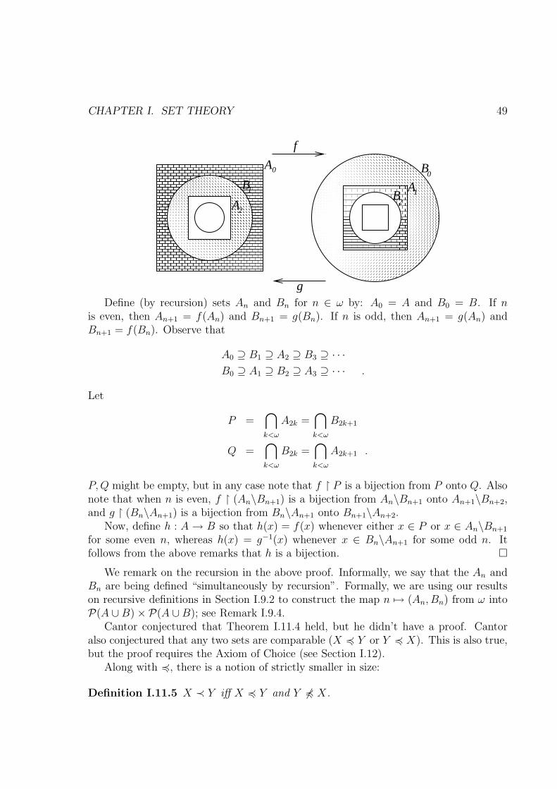
CHAPTER I. SET THEORY 49
��������������������������������������������������������������������������������������������������������������������������������������������������������������������������������������������������������������������������������������������������������������������������������������������������������������������������������������������������������������������������������������������
��������������������������������������������������������������������������������������������������������������������������������������������������������������������������������������������������������������������������������������������������������������������������������������������������������������������������������������������������������������������������������������������
��������������������������������������������������������������������������������������������������������������������������������������������������������������������������������������������������������������������������������������������������������������������������������������������������������������������������������������������������������������������������������������������������������������������������������������������������������������������������������������������������������������������������������������������������������������������������������������������������������������������������������������������������������������������������������������������������������������������������������������������������������������������������������������������������������������������������������������������������������������������������������������������������������������������������������������������������������������������������������������������������������������������������������������������������������������������������������������������������
��������������������������������������������������������������������������������������������������������������������������������������������������������������������������������������������������������������������������������������������������������������������������������������������������������������������������������������������������������������������������������������������������������������������������������������������������������������������������������������������������������������������������������������������������������������������������������������������������������������������������������������������������������������������������������������������������������������������������������������������������������������������������������������������������������������������������������������������������������������������������������������������������������������������������������������������������������������������������������������������������������������������������������������������������������������������������������������������������
�����������������������������������������������������������������������������������������������������������������������������������������������������������������������������������������������������������������������������������������������������������������������������������������������������������������������������������������������������������������������������������������������������������������������������������������������������������������������������������������������������������������������������������������������
�����������������������������������������������������������������������������������������������������������������������������������������������������������������������������������������������������������������������������������������������������������������������������������������������������������������������������������������������������������������������������������������������������������������������������������������������������������������������������������������������������������������������������������������������
������������������������������������������������������������������������������������������������������������������������������������������������������������
������������������������������������������������������������������������������������������������������������������������������������������������������������
f
g
1
A
B
A2
0 B0
A1B2
Define (by recursion) sets An and Bn for n ∈ ω by: A0 = A and B0 = B. If nis even, then An+1 = f(An) and Bn+1 = g(Bn). If n is odd, then An+1 = g(An) andBn+1 = f(Bn). Observe that
A0 ⊇ B1 ⊇ A2 ⊇ B3 ⊇ · · ·B0 ⊇ A1 ⊇ B2 ⊇ A3 ⊇ · · · .
Let
P =⋂
k<ω
A2k =⋂
k<ω
B2k+1
Q =⋂
k<ω
B2k =⋂
k<ω
A2k+1 .
P,Q might be empty, but in any case note that f ↾ P is a bijection from P onto Q. Alsonote that when n is even, f ↾ (An\Bn+1) is a bijection from An\Bn+1 onto An+1\Bn+2,and g ↾ (Bn\An+1) is a bijection from Bn\An+1 onto Bn+1\An+2.
Now, define h : A→ B so that h(x) = f(x) whenever either x ∈ P or x ∈ An\Bn+1
for some even n, whereas h(x) = g−1(x) whenever x ∈ Bn\An+1 for some odd n. Itfollows from the above remarks that h is a bijection. �
We remark on the recursion in the above proof. Informally, we say that the An andBn are being defined “simultaneously by recursion”. Formally, we are using our resultson recursive definitions in Section I.9.2 to construct the map n 7→ (An, Bn) from ω intoP(A ∪B)×P(A ∪B); see Remark I.9.4.
Cantor conjectured that Theorem I.11.4 held, but he didn’t have a proof. Cantoralso conjectured that any two sets are comparable (X 4 Y or Y 4 X). This is also true,but the proof requires the Axiom of Choice (see Section I.12).
Along with 4, there is a notion of strictly smaller in size:
Definition I.11.5 X ≺ Y iff X 4 Y and Y 64 X.
CHAPTER I. SET THEORY 50
In view of the Schroder-Bernstein Theorem, this is the same as saying that X can bemapped 1-1 into Y , but there is no bijection from X onto Y .
A famous theorem of Cantor states that A ≺ P(A). We isolate the key idea of theproof, showing that one cannot map A onto P(A), as:
Lemma I.11.6 (Cantor’s Diagonal Argument) If f is a function, dom(f) = A,and D = {x ∈ A : x /∈ f(x)}, then D /∈ ran(f).
Proof. If D = f(c) for some c ∈ A, then applying the definition of D with x = c wewould have c ∈ D ↔ c /∈ f(c), so c ∈ D ↔ c /∈ D, a contradiction. �
Theorem I.11.7 (Cantor) A ≺ P(A).
Proof. A 4 P(A) because the map x 7→ {x} defines an injection from A to P(A).P(A) 64 A because if P(A) 4 A, then there would be a a bijection from A onto P(A),contradicting Lemma I.11.6. �
Applying this theorem with A = V = {x : x = x}, we get
Paradox I.11.8 (Cantor) V ≺ P(V ); but P(V ) = V , so V ≺ V , a contradiction.
Of course, the upshot of this “contradiction” is that there is no universal set, whichwe already know (Theorem I.6.6), and proved much more simply using Russell’s Paradox.Note that Russell’s Paradox is just a special case of the diagonal argument: If we applythe proof of Lemma I.11.6 with A = V = P(V ) and f the identity function (so D = c),we get D = {x : x /∈ x}, yielding the contradiction D ∈ D ↔ D /∈ D.
The power set operation thus yields larger and larger cardinalities. This is a specialcase of exponentiation.
Lemma I.11.9 A2 ≈ P(A).
Proof. 2 = {0, 1}, so associate a subset of A with its characteristic function. �
It is also easy to see:
Exercise I.11.10 If A 4 B and C 4 D then AC 4 BD. If 2 4 C then A ≺ P(A) 4 AC.
The detailed study of cardinal exponentiation will be taken up in Section I.13, usingthe Axiom of Choice, but without Choice, it is easy to verify the analogs to the familiarlaws of exponentiation for natural numbers: (xy)z = xy·z and x(y+z) = xy · xz.
Lemma I.11.11
1. C(BA) ≈ C×BA
2. (B∪C)A ≈ BA× CA if B,C are disjoint.

CHAPTER I. SET THEORY 51
Proof. For (1), define Φ : C(BA) −→1−1onto
C×BA by saying that Φ(f)(c, b) = (f(c))(b). For(2), define Ψ : (B∪C)A −→1−1
ontoBA × CA by saying that Ψ(f) = (f↾B, f↾C). Of course, for
both Φ,Ψ, one must check that their definitions make sense and that they really arebijections. �
Φ and Ψ are actually “natural” in many settings, where A has some structure on it andexponentiation is defined. For example, if A is a group, and we use the standard groupproduct, then the Φ and Ψ are group isomorphisms. Also, if A is a topological space andwe use the standard (Tychonov) product topology, then Φ and Ψ are homeomorphisms.
Definition I.11.12 A is countable iff A 4 ω. A is finite iff A 4 n for some n ∈ ω.“ infinite” means “not finite”. “ uncountable” means “not countable”. A is countablyinfinite iff A is countable and infinite.
By Theorem I.11.7, P(ω) is uncountable. It is easy to prove that P(ω) ≈ R ≈ C,once R and C have been defined (see Section I.15). We say that the sets P(ω),R,C havesize continuum, since R is sometimes referred to as the continuum of real numbers. Thefollowing continuation of Exercise I.8.23 is useful when dealing with sizes of sets:
Exercise I.11.13
1. B ⊆ α→ type(B;∈) ≤ α.
2. If B 4 α then B ≈ δ for some δ ≤ α.
3. If α ≤ β ≤ γ and α ≈ γ then α ≈ β ≈ γ.
By (3), the ordinals come in blocks of the same size or cardinality. The first ordinalin its block is called a cardinal (or a cardinal number). In English grammar, the words“two, three, four” are called cardinal numbers (denoting magnitudes), whereas the words“second, third, fourth” are called ordinal numbers (and are used in concepts involvingordering or sequences). In set theory, they just become the same 2, 3, 4. However, in theinfinite case, one distinguishes between ordinals and cardinals:
Definition I.11.14 A (von Neumann) cardinal is an ordinal α such that ξ ≺ α for allξ < α.
Since ξ < α → ξ ⊆ α → ξ 4 α, an ordinal α fails to be a cardinal iff there is someξ < α with ξ ≈ α.
Theorem I.11.15
1. Every cardinal ≥ ω is a limit ordinal.
2. Every natural number is a cardinal.
3. If A is a set of cardinals, then sup(A) is a cardinal.
4. ω is a cardinal.
CHAPTER I. SET THEORY 52
Proof. For (1), assume that α ≥ ω and α = δ + 1 (so α > δ ≥ ω). Then α cannotbe a cardinal because we can define a bijection f from α = δ ∪ {δ} onto δ by: f(δ) = 0,f(n) = n+ 1 for n ∈ ω ⊆ δ, and f(ξ) = ξ whenever ω ≤ ξ < δ.
For (2), use ordinary induction (Theorem I.8.14): 0 is a cardinal because DefinitionI.11.14 is vacuous for α = 0. So, we assume that n is a cardinal, and prove that S(n) isa cardinal. If not, fix ξ < S(n) such that ξ ≈ S(n). Let f : ξ −→1−1
onto S(n) = n ∪ {n}. Ifξ = ∅, this is impossible, so let ξ = S(m), where m < n. Then f : m∪{m} −→1−1
onto n∪{n}.If f(m) = n, then f↾m : m −→1−1
onto n, contradicting the assumption that n is a cardinal. Iff(m) = j < n, then fix i < m such that f(i) = n. But then, if we define g : m → n sothat g(x) = f(x) unless x = i, in which case g(x) = j, then g is a bijection, so we havethe same contradiction.
For (3), if supA =⋃A fails to be a cardinal, fix some ξ < supA such that ξ ≈ supA.
Now, fix α ∈ A such that ξ < α. Then ξ ≈ α by Exercise I.11.13, contradicting theassumption that all elements of A are cardinals.
(4) is immediate from (2) and (3), setting A = ω. �
Now, we would like to define |A| to be the cardinal κ such that A ≈ κ. However,to prove that there is such a κ requires well-ordering A, which requires the Axiom ofChoice (AC) (see Section I.12).
Definition I.11.16 A set A is well-orderable iff there is some relation R which well-orders A.
Exercise I.11.17 A can be well-ordered in type α iff there is a bijection f : A −→1−1onto α.
Hence, A is well-orderable iff A ≈ α for some ordinal α.
Definition I.11.18 If A is well-orderable, then |A| is the least ordinal α such that A ≈α.
Clearly, every set of ordinals is well-orderable. In particular, |α| is defined for all α.It is easy to see directly that |ω + ω| = ω; more generally, ordinal arithmetic applied toinfinite ordinals does not raise the cardinality (see Exercise I.11.34).
Exercise I.11.19 If A is well-orderable and f : A−→onto B, then B is well-orderable and|B| ≤ |A|.
Exercise I.11.20 If κ is a cardinal and B is a non-empty set, then B 4 κ iff there isa function f : κ−→onto B.
In particular, with κ = ω, a non-empty B is countable by Definition I.11.12 (i.e.,B 4 ω) iff there is a function f : ω−→onto B; that is, you can count B using the naturalnumbers.
Exercise I.11.21 Assume that A,B are well-orderable. Then:
CHAPTER I. SET THEORY 53
✌ |A| is a cardinal.
✌ A 4 B iff |A| ≤ |B|.✌ A ≈ B iff |A| = |B|.✌ A ≺ B iff |A| < |B|.
Exercise I.11.22 A is finite iff A is well-orderable and |A| < ω
Exercise I.11.23 If A and B are finite, then A ∪B and A× B are finite.
Hint. For m,n < ω, first show m+ n < ω by induction on n, and then show m · n < ωby induction on n. �
We have not yet produced an uncountable cardinal. We have produced uncountablesets, such as P(ω). AC is equivalent to the statement that all sets are well-orderable(see Section I.12), so under AC, the continuum |P(ω)| is an uncountable cardinal. ByCohen [6, 7] (or, see [18]), ZF does not prove that P(ω) is well-orderable. However bythe following argument, one can produce uncountable cardinals without using AC.
Theorem I.11.24 (Hartogs, 1915) For every set A, there is a cardinal κ such thatκ 64 A.
Proof. Let W be the set of pairs (X,R) ∈ P(A)×P(A×A) such that R ⊆ X ×X andR well-orders X. So, W is the set of all well-orderings of all subsets of A. Observe thatα 4 X iff α = type(X;R) for some (X,R) ∈ W (see Exercise I.11.17). Applying theReplacement Axiom, we can set β = sup{type(X,R) + 1 : (X,R) ∈ W}. Then β > αwhenever α 4 A, so β 64 A. Let κ = |β|. Then κ ≈ β, so κ 64 A. �
Definition I.11.25 ℵ(A) is the least cardinal κ such that κ 64 A. For ordinals, α,α+ = ℵ(α).
Exercise I.11.26 For ordinals, α, α+ is the least cardinal greater than α.
Exercise I.11.27 The β occurring in the proof of Theorem I.11.24 is already a cardinal.So, β = κ = ℵ(A), and ℵ(A) is |A|+ 1 when A is finite and |A|+ when A is infinite andwell-orderable.
This ℵ(A) is the Hartogs aleph function. It is used most frequently when working inset theory without the Axiom of Choice. Under AC, |A| is always defined, and ℵ(A) isthe same as |A|+, which is the more standard notation.
Applying transfinite recursion:
Definition I.11.28 The ℵξ = ωξ are defined by recursion on ξ by:
• ℵ0 = ω0 = ω.

CHAPTER I. SET THEORY 54
• ℵξ+1 = ωξ+1 = (ℵξ)+.
• ℵη = ωη = sup{ℵξ : ξ < η} when η is a limit ordinal.
Frequently, “ℵξ” is used when talking about cardinalities and “ωξ” is used whentalking about order types. The ℵξ list the infinite cardinals in increasing order:
Exercise I.11.29 ξ < ζ → ℵξ < ℵζ . κ is an infinite cardinal iff κ = ℵξ for some ξ.
AC is required to get a reasonable theory of cardinals, but some elementary facts canbe proved just in ZF . For example, we already know that α × α can be well-orderedlexicographically. The type is, by definition, α · α, which is greater than α wheneverα ≥ 2. However, the cardinality is the same as that of α whenever α is infinite; inparticular, ω × ω is countably infinite:
Theorem I.11.30 If α ≥ ω then |α × α| = |α|. Hence, if κ ≥ ω is a cardinal, then|κ× κ| = κ.
Proof. It is sufficient to prove the statement for cardinals, since then, with κ = |α|, wewould have α × α ≈ κ × κ ≈ κ ≈ α. Note that κ 4 κ × κ via the map ξ 7→ (ξ, ξ), butwe need to show that |κ× κ| can’t be bigger than κ.
We shall define a relation ⊳ on ON × ON which well-orders ON × ON , and thenprove that it well-orders κ × κ in order type κ whenever κ is an infinite cardinal. Thiswill yield κ× κ ≈ κ.
Define (ξ1, ξ2) ⊳ (η1, η2) to hold iff either max(ξ1, ξ2) < max(η1, η2) or we have bothmax(ξ1, ξ2) = max(η1, η2) and (ξ1, ξ2) precedes (η1, η2) lexicographically. It is easy toverify that ⊳ well-orders ON × ON (in the same sense that ∈ well-orders ON ; seeTheorem I.8.5). If S is a subset of ON × ON , then type(S) denotes type(S,⊳). Forexample, type((ω + 1)× (ω + 1)) = ω · 3 + 1.
We now need to verify that type(κ× κ) = κ whenever κ is an infinite cardinal. Weproceed by transfinite induction (using Theorem I.9.1). So, assume that κ is the leastinfinite cardinal such that δ := type(κ× κ) 6= κ, and we derive a contradiction.
If α < κ is any ordinal, then |α × α| < κ: If α is infinite, this follows because κis least, so type(|α| × |α|) = |α|, and hence |α| × |α| ≈ |α|; since |α| ≈ α, we haveα× α ≈ α < κ. If α is finite, then |α× α| < ω ≤ κ, by Exercise I.11.23.
Now, let F : δ −→1−1onto κ× κ be the isomorphism from (δ;<) to (κ× κ;⊳).
If δ > κ, let (ξ1, ξ2) = F (κ), and let α = max(ξ1, ξ2) + 1. Then α < κ because κ isa limit ordinal (Theorem I.11.15), and F“κ ⊆ α × α by the definition of ⊳, so we haveκ 4 α× α ≺ κ, a contradiction.
If δ < κ, then κ 4 κ×κ ≈ δ ≺ κ (since κ is a cardinal), again a contradiction. Thus,δ = κ. �
Exercise I.11.31 Every countable strict total ordering is isomorphic to a subset of Q.

CHAPTER I. SET THEORY 55
Exercise I.11.32 The following are equivalent for an ordinal α:
1. α is isomorphic to a subset of Q.
2. α is isomorphic to a subset of R.
3. α is countable.
4. α is isomorphic to a subset of Q which is closed as a subset of R.
Hint. Of course, we haven’t officially defined Q, R yet. (4) → (1) → (2) is trivial.(3) → (4) is done by induction on α (see Subsection I.7.3 for α = ω2). (2) → (3) holdsbecause an uncountable well-ordered subset of R would yield an uncountable family ofdisjoint open intervals, which is impossible because Q is countable and dense in R.
Regarding (4), say α ∼= K ⊂ R, where K is closed. If α is a limit ordinal, then Kis unbounded in R, while if α is a successor, then K is bounded, and hence compact.A somewhat harder exercise is to show that if X is any compact Hausdorff space and0 < |X| ≤ ℵ0, then X is homeomorphic to some successor ordinal. �
Exercise I.11.33 Let δ = δ0 be any ordinal, and let δn+1 = ℵδn. Let γ = sup{δn : n ∈ω}. Show that ℵγ = γ. Furthermore, if δ0 = 0, then γ is the least ordinal ξ such thatℵξ = ξ.
Exercise I.11.34 Ordinal arithmetic doesn’t raise cardinality. That is, assume that α, βare ordinals with 2 ≤ min(α, β) and ω ≤ max(α, β). Then prove that |α+ β| = |α · β| =|αβ| = max(|α|, |β|).
Hint. For α + β and α · β, this is easy from Theorem I.11.30 and the definitions of+ and ·. The proof is slightly tricky for exponentiation, since the natural proof byinduction on β seems to use the Axiom of Choice (AC). Here, we take the recursivecomputation in Table I.1 to be the definition of αβ. Now, say we want to prove byinduction on β that αβ is countable whenever α, β are countable. If β is a limit, wehave αβ = supξ<β(αξ) =
⋃ξ<β(αξ) which (applying induction) is a countable union of
countable sets. But the well-known fact that a countable union of countable sets iscountable (Theorem I.12.12) uses AC. To avoid AC, first fix a δ < ω1 and then fix anf : δ−→1−1 ω. Now, we may now define, for α, β < δ, an injection from αβ into ω; thedefinition uses f , and is done by recursion on β; the definition also uses a (fixed) injectionfrom ω × ω into ω.
A similar method of proof shows in ZF that other ordinal arithmetic functions definedby recursion don’t raise cardinality. For example, we may define a hyperexponential func-
tion h so that h(α, 3) = αααα
: h(α, 0) = α ; h(α, S(β)) = αh(α,β) ; h(αγ) = supβ<γ h(α, β)for γ a limit. Then h(α, β) is countable when α, β are countable. �
Exercise I.11.35 Prove within the theory Z− (see Section I.2 ) that there is an uncount-able well-ordered set.

CHAPTER I. SET THEORY 56
Hint. Let A = ω and then form W as in the proof of Theorem I.11.24. Let B = W/∼=,where ∼= is the isomorphism relation, and define an appropriate well-order on B. SeeExercise I.10.5 for some historical remarks, and for how to construct a quotient withoutusing the Axiom of Replacement. Note that Hartogs in 1915 could not have statedTheorem I.11.24 as we did here, since this was before von Neumann ordinals (1923) andthe introduction of the Axiom of Replacement (1922). �
I.12 The Axiom of Choice (AC)
There are many known equivalents to AC. For a detailed discussion, see Howard andRubin [16]. We confine ourselves here to the versions of AC most likely to be useful inmathematics. This boils down to:
Theorem I.12.1 (ZF) The following are equivalent
1. The Axiom of Choice (as in Section I.2 ).
2. Every set has a choice function.
3. Every set can be well-ordered.
4. ∀xy(x 4 y ∨ y 4 x).
5. Tukey’s Lemma.
6. The Hausdorff Maximal Principle.
7. Zorn’s Lemma.
(2) (5) (6) (7) will be defined in this section, and proofs of equivalence given, althoughthe equivalences involving (6) and (7) will be left to the exercises; these two are importantand well-known, but they are never used in this book, except in the exercises.
The form of AC in Section I.2 was used because it requires few definitions to state:
∅ /∈ F ∧ ∀x ∈ F ∀y ∈ F (x 6= y → x ∩ y = ∅) → ∃C ∀x ∈ F (SING(C ∩ x))
That is, whenever F is a disjoint family of non-empty sets, there is a set C such thatC ∩ x is a singleton set for all x ∈ F . C is called a choice set for F because it choosesone element from each set in x. If you draw a picture, this principle will seem “obviouslytrue”, although, since F may be infinite, it needs to be stated as a separate principle (asobserved by Zermelo (1908), and proved by Cohen (1963)).
In practice, this version is not very useful, since one frequently needs to chooseelements from sets which are not disjoint, in which case one must do the choosing by achoice function:
Definition I.12.2 A choice function for a set A is a function g : P(A) \ {∅} → A suchthat g(x) ∈ x for all x ∈ P(A) \ {∅}.
CHAPTER I. SET THEORY 57
Proof of Theorem I.12.1 (1)↔ (2) .For (2) → (1): Given a disjoint family F of non-empty sets: Let A =
⋃F , let g be
a choice function for A, and let C = {g(x) : x ∈ F}.For (1) → (2): Given any set A, let F = {{x} × x : x ∈ P(A) \ {∅}}. By this trick,
we take each non-empty x ⊆ A and form a copy of it, {x} × x = {(x, i) : i ∈ x}. Ifx 6= y, then {x} × x and {y} × y are disjoint. Hence, by (1), there is a choice set C forF . But then C : P(A) \ {∅} → A is a choice function for A. �
A choice function g for A gives you a way to well-order A. Informally, we list A in atransfinite sequence as described in Section I.5:
a0, a1, a2, a3, . . . . . . . . .
Get a0 by choosing some element of A, then choose some a1 different from a0, thenchoose some a2 different from a0, a1, then choose some a3 different from a0, a1, a2, andso on. If A is infinite, this will require an infinite number of choices, and the “choosing”is justified formally by a choice function g:
Proof of Theorem I.12.1 (2)↔ (3)↔ (4) .For (3) → (2): If R well-orders A, we can define a choice function g by letting g(x)
be the R-least element of x.For (2) → (3): Conversely, let g be a choice function for A. Fix κ = ℵ(A). Fix
any S /∈ A. Think of S as signifying “Stop”. Define f : κ → A ∪ {S} so that f(α) =g(A \ {f(ξ) : ξ < α}) if A \ {f(ξ) : ξ < α} is non-empty; otherwise, f(α) = S. Observethat f(ξ) 6= f(α) whenever ξ < α and f(α) 6= S. Since κ 64 A, there can be nof : κ−→1−1 A, so f(α) = S for some α. Now, let α be least such that f(α) = S, and notethat f ↾ α : α −→1−1
onto A; thus, A can be well-ordered in type α (see Exercise I.11.17).For (4) → (3): If κ = ℵ(A), then κ 64 A, so (4) implies that A 4 κ, so A can be
well-ordered (see Exercise I.11.13).For (3) → (4): If x and y can be well-ordered, then |x| and |y| are von Neumann
cardinals, and |x| ≤ |y| or |y| ≤ |x|. �
Note that we have actually shown, for each fixed set A, that A is well-orderable iff Ahas a choice function.
We have now shown the equivalence of (1), (2), (3), (4) of Theorem I.12.1. The otherthree principles are all maximal principles. The most well-known among these is (7),Zorn’s Lemma. This is often quoted, for example, in the proof that every vector spacehas a basis. However, in many of the elementary applications, such as this one, Tukey’sLemma (5) is a more convenient maximal principle to use, so we shall begin with (5),which involves the existence of a maximal set in a family of sets:
Definition I.12.3 If F ⊆ P(A), then X ∈ F is maximal in F iff it is maximal withrespect to the relation $ (see Definition I.7.19 ); that is, X is not a proper subset of anyset in F .

CHAPTER I. SET THEORY 58
Some examples: If F = P(A), then A is maximal in F . If F is the set of finitesubsets of A, and A is infinite, then F has no maximal element. A less trivial exampleis:
Example I.12.4 Let A be any vector space over some field. Define F ⊆ P(A) so thatX ∈ F iff X is linearly independent. Then X is maximal in F iff X is a basis.
The proof of this is an easy exercise in linear algebra, and does not use the Ax-iom of Choice. Note that linearly independent means that there is no set of vectors{x1, . . . , xn} ⊆ X (where 1 ≤ n < ω) and non-zero scalars a1, . . . , an in the field suchthat a1x1 + · · ·+ anxn = 0. If X is linearly independent and is not a basis (that is, failsto span A), then there is some y ∈ A which is not in the linear span of X, which implies(by linear algebra) that X ∪ {y} is also linearly independent, so X is not maximal.
The feature which implies that this particular F has a maximal element is that F isof finite character.
Definition I.12.5 F ⊆ P(A) is of finite character iff for all X ⊆ A: X ∈ F iff everyfinite subset of X is in F .
Exercise I.12.6 If F is of finite character, X ∈ F , and Y ⊆ X, then Y ∈ F .
Definition I.12.7 Tukey’s Lemma is the assertion that whenever F ⊆ P(A) is of finitecharacter and X ∈ F , there is a maximal Y ∈ F such that X ⊆ Y .
The F in Example I.12.4 is of finite character because the notion of “linearly in-dependent” is verified by looking only at finite subsets of X. Hence, Tukey’s Lemmaimplies that every vector space has a basis. Here, as in many applications, X can be∅. Applying Tukey’s Lemma with an arbitrary X shows that every linearly independentset can be expanded to a basis.
This type of proof is common in undergraduate texts. The advantage of it is that youcan follow the proof without having to know about ordinals and transfinite recursion;Tukey’s Lemma or Zorn’s Lemma can be taken as an axiom. The disadvantage is thatthese maximal principles are a bit complicated, and it’s hard to explain why they shouldbe axioms. The standard choice versions of AC, (1) or (2), have a much clearer intuitivemotivation. Of course, once you know about ordinals and recursion, the proof of Tukey’slemma is quite simple:
Proof of Theorem I.12.1 (3)→ (5)→ (1) .For (3) → (5): Fix A,F , X as in Definition I.12.7. Since A can be well-ordered, we
can list A as {xα : α < κ}, where κ = |A|. Recursively define Yβ ⊆ {xξ : ξ < β}, forβ ≤ κ, by:
a. Y0 = X.
b. Yα+1 is Yα ∪ {xα} if Yα ∪ {xα} ∈ F ; otherwise, Yα+1 = Yα.

CHAPTER I. SET THEORY 59
c. Yγ =⋃{Yα : α < γ} if γ is a limit ordinal.
Now, check, inductively, that Yβ ∈ F for each β ≤ κ. For the successor step, use (b).For limit β, use (c) and the fact that F is of finite character. Let Y = Yκ. Then Y ∈ F .To see that Y is maximal, fix xα /∈ Y . Then, by (b), Yα ∪ {xα} /∈ F , so the supersetY ∪ {xα} is also not in F (see Exercise I.12.6).
For (5)→ (1): Let F be any family of disjoint non-empty sets. We need to producea choice set C, which intersects each z ∈ F in a singleton. Let A =
⋃F . Let G be the
set of all partial choice sets for F ; so X ∈ G iff X ∈ P(A) and X ∩ z is either a singletonor empty for all z ∈ F . G is of finite character because if X ⊆ A fails to be in G, thensome two-element subset of X fails to be in G. Also, ∅ ∈ G, so applying Tukey’s Lemma,fix a maximal C ∈ G. If C is not a choice set for F , we can fix a z ∈ F such that C ∩ zis not a singleton, and is hence empty (since C ∈ G). But then, since z 6= ∅, we can fixp ∈ z and note that C $ C ∪ {p} ∈ G, contradicting maximality. �
We have now proved the equivalence of (1), (2), (3), (4), (5), in Theorem I.12.1. Weshall now state (6) and (7), and leave the proofs of equivalence to the exercises. Boththese equivalents involve partial orders. We shall phrase these in terms of strict partialorders < (as in Definition I.7.2); then x ≤ y abbreviates x < y ∨ x = y.
Definition I.12.8 Let < be a strict partial order of a set A. Then C ⊆ A is a chainiff C is totally ordered by <; C is a maximal chain iff in addition, there are no chainsX % C.
Definition I.12.9 The Hausdorff Maximal Principle is the assertion that whenever <is a strict partial order of a set A, there is a maximal chain C ⊆ A.
Definition I.12.10 Zorn’s Lemma is the assertion that whenever < is a strict partialorder of a set A satisfying
(✌) For all chains C ⊆ A there is some b ∈ A such that x ≤ b for all x ∈ C,
then for all a ∈ A, there is a maximal (see Definition I.7.19 ) b ∈ A with b ≥ a.
Exercise I.12.11 Finish the proof of Theorem I.12.1.
Hint. One way to do this is to show (5) → (6) → (7) → (5); this stays within themaximal principles. For (5)→ (6), note that the family of all chains has finite character.For (6)→ (7), fix a maximal chain C containing a; then the b we get in (✌) is a maximalelement. For (7)→ (5), observe that if F is of finite character, then F , partially orderedby $, satisfies the hypothesis (✌) of Zorn’s Lemma. �
In “pure” set theory, the most frequently used forms of the Axiom of Choice are (2),guaranteeing the existence of choice functions, and (3) (the well-ordering principle). Inalgebra, analysis, and model theory, frequent use is made of Zorn’s Lemma (7) and/or
CHAPTER I. SET THEORY 60
Tukey’s Lemma (5) as well. Often, Tukey’s Lemma is easier to apply, since one has afamily which is obviously of finite character, as in Example I.12.4. However, there aresome cases, such as Exercise I.12.14 below, where Zorn’s Lemma is more useful.
Texts in algebra and analysis usually point out the use of AC when they prove thatevery vector space has a basis or that there is a subset of R which is not Lebesguemeasurable. However, some more elementary uses of AC are often glossed over withoutexplicit mention. For example:
1. In elementary calculus, you learn that if 0 is a limit point of a set X of reals,then there is a sequence 〈xn : n ∈ ω〉 from X converging to 0. The usual proof choosesxn ∈ X ∩ (−1/n, 1/n). It is known to be consistent with ZF to have an X dense in Rwith ω 64 X, so all ω-sequences from X are eventually constant.
2. A countable union of countable sets is countable. This is true under AC (seeTheorem I.12.12 below). It is consistent with ZF that R is a countable union of countablesets; it is also consistent that ω1 is a countable union of countable sets; see [19] for moreon consistency results involving ¬AC.
Theorem I.12.12 (AC) Let κ be an infinite cardinal. If F is a family of sets with|F| ≤ κ and |X| ≤ κ for all X ∈ F , then |⋃F| ≤ κ.
Proof. Assume F 6= ∅ (otherwise the result is trivial) and ∅ /∈ F (since removing ∅ fromF does not change the union). Then (see Exercise I.11.20), fix f : κ−→onto F . Likewise, foreach B ∈ F , there are functions g : κ−→onto B. By AC, choose gα : κ−→onto f(α) for all α < κ(to do this, well-order S := κ(
⋃F), and let gα be the least g ∈ S with ran(g) = f(α)).This defines h : κ×κ−→onto
⋃F , where h(α, β) = gf(α)(β). Since |κ×κ| = κ (see TheoremI.11.30), we can map κ onto
⋃F , so |⋃F| ≤ κ (see Exercise I.11.20). �
Informally, it’s “obvious” that if you have a map f : A−→onto B, then A must be atleast as large as B (i.e., B 4 A), but producing a g : B−→1−1 A requires AC. Concretely,ZF does not prove that there is an injection from ω1 into P(ω), but
Exercise I.12.13 Prove, without using AC, that one can map P(ω) onto ω1.
Hint. First, define f : P(ω × ω)−→onto ω1\ω so that f(R) = type(R) whenever R is awell-order of ω. �
Exercise I.12.14 If X, Y are compact Hausdorff spaces, a continuous map f : X → Yis called irreducible iff f : X −→onto Y , but f(H) 6= Y for all proper closed subsets H of X.For example, if Y = [0, 2] ⊂ R and X = [0, 1] × {0} ∪ [1, 2] × {1} ⊂ R × R, then theusual projection map is irreducible. Now, fix any continuous f : X −→onto Y , and prove thatthere is a closed Z ⊆ X such that f↾Z : Z −→onto Y and f↾Z is irreducible.
Hint. Use Zorn’s Lemma and get Z minimal in the set of all closed Z ⊆ X such thatf↾Z is onto. See Engelking’s text [11] for more on the use of irreducible maps in generaltopology. �
CHAPTER I. SET THEORY 61
I.13 Cardinal Arithmetic
In this section, we assume AC throughout. Then, since every set can be well-ordered,|x| is defined for all x. We define cardinal addition, multiplication, and exponentiationby:
Definition I.13.1 If κ, λ are cardinals, then
• κ+ λ = |{0} × κ ∪ {1} × λ|• κ · λ = |κ× λ|• κλ = |λκ|
The boxes are omitted when it is clear from context that cardinal arithmetic is intended.In particular, if a cardinal is listed as “ℵα”, then cardinal arithmetic is intended.
In the literature, boxes are never used, and the reader must determine from contextwhether ordinal or cardinal arithmetic is intended. The context is important becausethere are three possible meanings to “κλ”, and all are used: the ordinal exponent, thecardinal exponent (i.e., κλ ), and the set of functions (i.e., λκ). To avoid too many boxesin our notation, we shall often phrase results by saying in English which operation isintended. This is done in the following two lemmas; the first says that the cardinalfunctions are monotonic in each argument; the second lists some elementary arithmeticfacts which are well-known for finite cardinals.
Lemma I.13.2 If κ, λ, κ′, λ′ are cardinals and κ ≤ κ′ and λ ≤ λ′, then κ+ λ ≤ κ′ + λ′,κ · λ ≤ κ′ · λ′, and κλ ≤ (κ′)λ
′
(unless κ = κ′ = λ = 0), where cardinal arithmetic ismeant throughout.
Proof. For the first two inequalities, use {0} × κ ∪ {1} × λ ⊆ {0} × κ′ ∪ {1} × λ′ and|κ× λ| ⊆ |κ′ × λ′|. For the third, when κ′ > 0, define ϕ : λκ−→1−1 (λ′)(κ′) by: ϕ(f)↾λ = fand (ϕ(f))(ξ) = 0 for λ ≤ ξ < λ′. When κ = κ′ = 0, note that 00 = |00| = |{∅}| = 1(the empty function maps ∅ to ∅), while for λ > 0, 0λ = |λ0| = |∅| = 0. �
Note that 00 = 1 in ordinal exponentiation as well.
Lemma I.13.3 If κ, λ, θ are cardinals, then using cardinal arithmetic throughout:
1. κ+ λ = λ+ κ.
2. κ · λ = λ · κ.
3. (κ+ λ) · θ = κ · θ + λ · θ.
4. κ(λ·θ) = (κλ)θ.
5. κ(λ+θ) = κλ · κθ.

CHAPTER I. SET THEORY 62
Proof. For (1,2,3), note that for any sets A,B,C: A∪B = B ∪A, A×B ≈ B×A, and(A ∪ B)× C = A× B ∪ A× C. For (4,5), apply Lemma I.11.11. �
We still need to use boxes in statements which involving both cardinal and ordinaloperations. An example is the following, which is immediate from the definitions of thecardinal and ordinal sum and product.
Lemma I.13.4 For any ordinals α, β: |α + β| = |α|+ |β| and |α · β| = |α| · |β| .
An example when α = β = ω = |ω|: ω, ω + ω, and ω · ω are three different ordinals,but these three ordinals have the same cardinality. This lemma fails for exponentiation,since (see Exercise I.11.34) ωω is a countable ordinal but ωω = (ℵ0)
ℵ0 = 2ℵ0 (by LemmaI.13.9), which is uncountable.
Lemma I.13.5 If κ, λ are finite cardinals, then κ+ λ = κ + λ, κ · λ = κ · λ, and
κλ = κλ.
Proof. Since finite ordinals are cardinals (by Theorem I.11.15), we have κ+λ = |κ+λ| =κ+ λ by Lemma I.13.4. The same argument works for product.
The fact that we know the lemma for sum and product lets us prove it for exponen-tiation by induction. The λ = 0 and λ = 1 cases are easy because κ0 = 1 and κ1 = κwith both cardinal and ordinal exponentiation. Now, assume we know that κλ = κλ; inparticular, κλ is finite. Now, since we already know that the cardinal and ordinal sumsand products agree for finite ordinals, Lemma I.13.3 gives us κλ+1 = κλ · κ. Since wealso know that κλ+1 = κλ · κ, we can conclude that κλ+1 = κλ+1. �
Lemma I.13.6 If κ, λ are cardinals and at least one of them is infinite, then κ+ λ =max(κ, λ). Also, if neither of them are 0 then κ · λ = max(κ, λ).
Proof. Assume that κ ≤ λ, so λ is infinite. It is clear from the definitions thatλ 4 κ+ λ 4 λ × λ, so use the fact that λ × λ ≈ λ (by Theorem I.11.30). The sameargument works for product when κ 6= 0. �
Because of these lemmas, cardinal sums and products are not very interesting, sincethey reduce to ordinal arithmetic for finite cardinals and they just compute the maxfor infinite cardinals; the sum and product notation is useful mainly for making generalstatements, such as Lemma I.13.3. Cardinal exponentiation, however, is of fundamentalimportance, since it is related to the Continuum Hypothesis. By Lemma I.11.9, andTheorem I.11.7, we have:
Lemma I.13.7 2κ = |P(κ)| for every cardinal κ, and 2ℵα ≥ ℵα+1 for every ordinal α.All exponentiation here is cardinal exponentiation.
CHAPTER I. SET THEORY 63
Definition I.13.8 The Continuum Hypothesis, CH , is the statement 2ℵ0 = ℵ1. TheGeneral Continuum Hypothesis, GCH , is the statement ∀α[2ℵα = ℵα+1]. All exponenti-ation here is cardinal exponentiation.
Knowing values of 2λ for the infinite λ tells us a lot about all the powers κλ. Inparticular, the GCH implies a very simple formula for κλ (see Theorem I.13.14), whichwe shall obtain by examining the possible cases. Of course, 1λ = 1. Also:
Lemma I.13.9 If 2 ≤ κ ≤ 2λ and λ is infinite, then κλ = 2λ. All exponentiation hereis cardinal exponentiation.
Proof. Applying Lemmas I.13.2, I.13.3, and I.13.6, we have 2λ ≤ κλ ≤ (2λ)λ = 2λ·λ = 2λ.�
So, infinite cardinal arithmetic is simpler than finite cardinal arithmetic. However,there are further complexities about κλ when λ < κ. Assuming GCH , Theorem I.13.14will yield (ℵ3)
ℵ0 = ℵ3 and (ℵω1)ℵ0 = ℵω1
, but (ℵω)ℵ0 = ℵω+1. The key feature about ℵωhere is that it has countable cofinality:
Definition I.13.10 If γ is any limit ordinal, then the cofinality of γ is
cf(γ) = min{type(X) : X ⊆ γ ∧ sup(X) = γ} .
γ is regular iff cf(γ) = γ.
For example, consider γ = ω2. There are many X ⊆ γ such that sup(X) = γ (thatis, X is unbounded in γ). ω ∪{ω ·n : n ∈ ω} is unbounded in γ and has order type ω · 2.The set {ω · n : n ∈ ω} is also unbounded in γ, and this one has order type ω. This ω isthe least possible order type since if X ⊆ γ is finite, then X has a largest element, so itcannot be unbounded. Thus, cf(γ) = ω. As an aid to computing cofinalities:
Lemma I.13.11 For any limit ordinal γ:
1. If A ⊆ γ and sup(A) = γ then cf(γ) = cf(type(A)).
2. cf(cf(γ)) = cf(γ), so cf(γ) is regular.
3. If γ is regular then γ is a cardinal.
4. ω ≤ cf(γ) ≤ |γ| ≤ γ
5. If γ = ℵα where α is either 0 or a successor, then γ is regular.
6. If γ = ℵα where α is a limit ordinal, then cf(γ) = cf(α).
Proof.For (1): Let α = type(A). Note that α is a limit ordinal since A is unbounded in
γ. Let f : α −→1−1onto A be the isomorphism from α onto A. To prove that cf(γ) ≤ cf(α),
note that if Y is an unbounded subset of α, then f“Y is an unbounded subset of γ of

CHAPTER I. SET THEORY 64
the same order type; in particular, taking Y to be of type cf(α) produces an unboundedsubset of γ of type cf(α). To prove that cf(α) ≤ cf(γ), fix an unbounded X ⊆ γ oforder type cf(γ). For ξ ∈ X, let h(ξ) be the least element of A which is ≥ ξ. Notethat ξ < η → h(ξ) ≤ h(η). Let X ′ = {η ∈ X : ∀ξ ∈ X ∩ η [h(ξ) < h(η)]}. Thenh↾X ′ : X ′−→1−1 A and h↾X ′ is order preserving. Also, h(X ′) is unbounded in A, whichhas order type α, so cf(α) ≤ type(X ′) ≤ type(X) = cf(γ) (using Exercise I.8.23).
For (2): Let A be an unbounded subset of γ of order type cf(γ), and apply (1).For (3): Suppose κ = |γ| < γ, and let f : κ−→onto γ; we show that cf(γ) ≤ κ. Define
(recursively) a function g : κ → ON so that g(η) = max(f(η), sup{g(ξ) + 1 : ξ < η}).Then ξ < η → g(ξ) < g(η), so g is an isomorphism onto its range. If ran(g) ⊆ γ, thenran(g) is a subset of γ of order type κ, and ran(g) is unbounded (since each g(η) ≥ f(η)),so cf(γ) ≤ κ. If ran(g) 6⊆ γ, let η be the least ordinal such that g(η) ≤ γ. Then η is alimit ordinal, since g(ξ+1) = max(g(ξ)+1, f(ξ+1)). Thus, g“η is an unbounded subsetof γ of order type η, so cf(γ) ≤ η < κ.
In (4), ω ≤ cf(γ) ≤ γ and |γ| ≤ γ are clear from the definitions, and cf(γ) ≤ |γ|follows from (2) and (3)
For (5): ℵ0 = ω is regular by (4). ℵβ+1 is regular because if A ⊆ ℵβ+1 and |A| ≤ ℵβ,then sup(A) =
⋃A is the union of ≤ ℵβ sets (ordinals), each of size ≤ ℵβ, so that
| sup(A)| ≤ ℵβ by Theorem I.12.12For (6): Apply (1), with A = {ℵξ : ξ < α}. �
By (1), cf(α + β) = β (let A = {α + ξ : ξ < β}). By (4), every limit ordinal belowω1 has cofinality ω. Likewise, every limit ordinal below ω2 has cofinality either ω (forexample, ω1 + ω) or ω1 (for example, ω1 + ω1).
By (3), regular ordinals are cardinals. The following fact about unions generalizesTheorem I.12.12 in the case that θ = κ+.
Theorem I.13.12 Let θ be any cardinal.
1. If θ is regular and F is a family of sets with |F| < θ and |S| < θ for all S ∈ F ,then |⋃F| < θ.
2. If cf(θ) = λ < θ, then there is a family F of subsets of θ with |F| = λ and⋃F = θ,
and |S| < θ for all S ∈ F .
Proof. For (1), let X = {|S| : S ∈ F}. Then X ⊆ θ and |X| < θ, so type(X) < θ, andhence sup(X) < θ. Let κ = max(sup(X), |F|) < θ. If κ is infinite, then by TheoremI.12.12, |⋃F| ≤ κ. If κ is finite, then
⋃F is finite. In either case, |⋃F| < θ.For (2), let F be a subset of θ of order type λ such that supF =
⋃F = λ. �
By generalizing Cantor’s diagonal argument for proving 2λ > λ, we get:
Theorem I.13.13 (Konig, 1905) If κ ≥ 2 and λ is infinite, then cf(κλ) > λ.
CHAPTER I. SET THEORY 65
Proof. Let θ = κλ, which must be infinite. Note that θλ = κλ·λ = κλ = θ. List λθ as{fα : α < θ}. If cf(θ) ≤ λ, we can write the ordinal θ as θ =
⋃ξ<λAξ, where |Aξ| < θ.
But now define g : λ → θ so that g(ξ) = min(θ \ {fα(ξ) : α ∈ Aξ}). Then g ∈ λθ and gdiffers from every fα, a contradiction. �
For example, cf(2ℵ0) > ω, so that 2ℵ0 cannot be ℵω. Roughly, it is consistent for 2ℵ0
to be any cardinal of uncountable cofinality, such as ℵ1 (CH ), or ℵ7, or ℵω+1, or ℵω1; see
[6, 7, 18, 20].The following lemma tells how to compute κλ under GCH when at least one of κ, λ
are infinite. It shows that it is the smallest possible value, given Konig’s Theorem. Weomit listing some trivial cases, when one of them is 0 or 1:
Theorem I.13.14 Assume GCH , and let κ, λ be cardinals with max(κ, λ) infinite.
1. If 2 ≤ κ ≤ λ+, then κλ = λ+.
2. If 1 ≤ λ ≤ κ, then κλ is κ if λ < cf(κ) and κ+ if λ ≥ cf(κ).
Proof. Part (1) is immediate from Lemma I.13.9. For (2), we have, applying GCH :κ ≤ λ ≤ κ ≤ κκ = 2κ = κ+, so κλ is either κ or κ+. If λ ≥ cf(κ), then κλ cannot be κby Konig’s Theorem, so it must be κ+. If λ < cf(κ), then every f : λ → κ is bounded,so that λκ =
⋃α<κ
λα. By GCH , each |λα| ≤ (max(|α|, λ))+ ≤ κ, so that |λκ| ≤ κ. �
We remark that (1) and (2) overlap slightly; if κ is either λ or λ+, then either appliesto show that κλ = λ+.
Analogously to Definition I.11.28:
Definition I.13.15 The iξ are defined by recursion on ξ by:
• i0 = ℵ0 = ω.
• iξ+1 = 2iξ.
• iη = sup{iξ : ξ < η} when η is a limit ordinal.
So, CH is equivalent to the statement that i1 = ℵ1 and GCH is equivalent to thestatement that iξ = ℵξ for all ξ.
Definition I.13.16 A cardinal κ is weakly inaccessible iff κ > ω, κ is regular, andκ > λ+ for all λ < κ. κ is strongly inaccessible iff κ > ω, κ is regular, and κ > 2λ forall λ < κ.
It is clear from the definitions that all strong inaccessibles are weak inaccessibles, andthat the two notions are equivalent under GCH . One cannot prove in ZFC that weakinaccessibles exist (see [18, 20]). By modifying Exercise I.11.33:
Exercise I.13.17 If κ is weakly inaccessible, then it is the κth element of {α : α = ℵα}.If κ is strongly inaccessible, then it is the κth element of {α : α = iα}.

CHAPTER I. SET THEORY 66
However, just in ZFC , the method of Exercise I.11.33 yields:
Exercise I.13.18 Prove that there is an α such that α = iα.
Following Erdos, we define:
Definition I.13.19 [A]κ = {x ⊆ A : |x| = κ} and [A]<κ = {x ⊆ A : |x| < κ}.
Exercise I.13.20 If λ is an infinite cardinal and κ ≤ λ is a cardinal, then |[λ]κ| = λκ.If 0 < κ ≤ λ then |[λ]<κ| = sup{λθ : θ = |θ| < κ}. In particular, |[λ]<ω| = λ.
Exercise I.13.21 Let λ be an infinite cardinal. Prove that there is a non-abelian groupof size λ and a field of size λ.
Hint. For example, you could use the free group on λ generators. You need somethinglike |[λ]<ω| = λ to show that this group has size λ. This exercise is trivial if you quotethe Lowenheim–Skolem Theorem (Theorem II.7.16), whose proof uses similar set theory,plus a lot of model theory. �
I.14 The Axiom of Foundation
The Axiom of Foundation was stated in Section I.2 just in terms of ∈ and =. However,it is clearly equivalent to:
∀x[x 6= ∅ → ∃y ∈ x(y ∩ x = ∅)] .
This axiom is completely irrelevant to the development of mathematics within settheory. Thus, it is reasonable to ask: What does it say and why is it on the list?
A brief answer is that it avoids “pathological sets” such as cycles in the ∈ relation.For example, if a ∈ a, then x = {a} is a counter-example to Foundation, since the onlymember of x is a, and x ∩ a = x 6= ∅. More generally, the ∈ relation can have no cycles,since if a1 ∈ a2 ∈ · · · ∈ an ∈ a1, then x = {a1, . . . , an} contradicts Foundation.
The Axiom of Extensionality excluded non-sets, such as badgers and ducks, from theset-theoretic universe under consideration (see Figure I.1, page 18). Then, the Axiomof Foundation excludes sets such that a ∈ a or b ∈ c ∈ b from the set-theoretic universeunder consideration (see Figure I.2, page 68). Neither Extensionality nor Foundationmakes any philosophical comment as to whether badgers or ducks or such sets a, b, creally exist in the “real world”, whatever that is.
Now, it turns out that sets such as these a, b, c never arise in the construction ofmathematical objects, so their existence has the same philosophical status as do ducksand badgers and trolls – they may exist or they may not exist, but their existencedoesn’t affect the mathematics. The purpose of this section is to make the informal “it

CHAPTER I. SET THEORY 67
turns out” into part of the theory. We define a subclass WF of V , the class of well-founded sets, and show that all mathematics takes place within WF . Then, Foundationis equivalent to the statement V = WF (see Theorem I.14.9). Foundation is never usedin the development of mathematics because mathematical objects, such as Q and R, arewell-founded anyway.
Roughly, the well-founded sets are those sets which can be obtained from nothing, ∅,by iterating collection that is, taking a bunch of sets and putting them between brackets,{· · · · · · }. Thinking of this as a construction, we start with ∅ at stage 0. At stage 1, wecan put brackets around it to form {∅} = 1. At stage 2, we already have constructed 0, 1,and we can form any of the four subsets of {0, 1}. Two of these, {0} = 1 and {} = ∅ = 0we already have. The two new ones are the rank 2 sets, shown in Table I.2.
Table I.2: The First Sixteen Sets
rank sets0 ∅ = 01 {∅} = 12 {{∅}} = {1} , {∅, {∅}} = 23 {{1}} , {0, {1}} , {1, {1}} , {0, 1, {1}} ,
{2} , {0, 2} , {1, 2} , {0, 1, 2} = 3 ,{{1}, 2} , {0, {1}, 2} , {1, {1}, 2} , {0, 1, {1}, 2}
At stage 3, we already have constructed 0, 1, 2, {1}, and we can form any of the24 = 16 subsets of {0, 1, 2, {1}}. Four of these we already have, and the 12 new ones arethe rank 3 sets. The 16 sets displayed in Table I.2 make up R(4), the collection of setswhose ranks are 0,1,2, or 3. This construction is generalized by:
Definition I.14.1 By recursion on α ∈ ON , define R(α) by:
1. R(0) = ∅.2. R(α + 1) = P(R(α)).
3. R(γ) =⋃α<γ R(α) for limit ordinals γ.
Then:
4. WF =⋃δ∈ON
R(δ) = the class of all well-founded sets.
5. The set x is well-founded iff ∃δ[x ∈ R(δ)].
6. For x ∈WF : rank(x) is the least α such that x ∈ R(α + 1).
WF is a proper class, since it contains all the ordinals (see Lemma I.14.5). Thus,WF does not really exist, but as with ON , the notation is useful. That is “x ∈WF ” isshorthand for “x is well-founded” and “x ⊆WF ” is shorthand for “∀y ∈ x∃δ[y ∈ R(δ)].Actually, item (6) of Definition I.14.1 needs some justification, given by:

CHAPTER I. SET THEORY 68
Lemma I.14.2 If x ∈WF , the least δ such that x ∈ R(δ) is a successor ordinal.
Proof. δ 6= 0 by item (1) and δ cannot be a limit ordinal by item (3). �
Figure I.2: The Set-Theoretic Universe in ZF
b
b
b
b
b
b
b
b
0
1
2
3
7
ω
ω + 1
α
b
b
b
b
b
b
b
b
b
b
b
b
b
b
−23
π Q
R
{1}
a
b c
the
wel
l-fo
unde
dse
ts
Note that |R(0)| = 0 and R(n + 1) has size 2|R(n)|, since R(n + 1) is the power setof R(n). Thus, |R(1)| = 20 = 1, |R(2)| = 21 = 2, |R(3)| = 22 = 4, |R(4)| = 24 = 16,|R(5)| = 216 = 65536, etc. The four elements of R(3) are the four elements of ranks 0,1 or 2. Of the 16 elements of R(4), four of them occur already in R(3); the other 12 donot, so they have rank 3.
Exercise I.14.3 List the 65520 sets of rank 4; this is easy to do with a computer programimplementing Exercise I.14.12.
Lemma I.14.4
1. Every R(β) is a transitive set.
2. α ≤ β → R(α) ⊆ R(β).

CHAPTER I. SET THEORY 69
3. R(α + 1) \R(α) = {x ∈WF : rank(x) = α}.4. R(α) = {x ∈WF : rank(x) < α}.5. If x ∈ y and y in WF , then x ∈WF and rank(x) < rank(y).
Proof. For (1), induct on β. If β = 0, then R(β) = 0, which is transitive. At limits, usethe fact that any union of transitive sets is transitive. Finally, assume R(β) is transitive;we shall prove that R(β + 1) is transitive. Note that R(β) ⊆ P(R(β)) = R(β + 1) sinceevery element of R(β) is a subset of R(β). Thus, if x ∈ R(β + 1) = P(R(β)), we havex ⊆ R(β) ⊆ R(β + 1), so R(β + 1) is transitive.
For (2), fix α and prove that R(α) ⊆ R(β) by induction on β ≥ α. It is trivial forβ = α, and the successor step follows from the fact that R(β) ⊆ R(β+ 1), which we justproved. If β > α is a limit, then R(β) =
⋃ξ<β R(ξ) ⊇ R(α).
(3) and (4) are immediate from (2) and the definition of rank. (5) is immediate from(3) and (4). �
Some of the elements of WF are shown in Figure I.2. These have been placed at theproper level to indicate their rank, and a few arrows have been inserted to indicate the∈ relation. Lemma I.14.4(5) says that WF is a transitive class and that the ∈–arrowsall slope upwards.
Table I.2 shows that the ordinals 0, 1, 2, 3 have ranks 0, 1, 2, 3, respectively. Thisgeneralizes:
Lemma I.14.5
1. ON ∩R(α) = α for each α ∈ ON .
2. ON ⊆WF
3. rank(α) = α for each α ∈ ON .
Proof. (1) is proved by induction on α. The cases where α is 0 or a limit are easy.Now, assume ON ∩R(α) = α. We show that ON ∩R(α+ 1) = α+ 1 = α∪ {α}. To seethat α∪{α} ⊆ R(α+ 1), note that α ⊆ R(α) ⊆ R(α+ 1) and α ∈ P(R(α)) = R(α+ 1).Now, let δ be any ordinal in R(α+ 1) = P(R(α)). Then δ ⊆ R(α) ∩ON = α, so δ ≤ α.Thus, ON ∩ R(α + 1) = {δ : δ ≤ α} = α + 1.
(1) implies that α ∈ R(α + 1) \R(α), which yields (2) and (3). �
To compute the rank of a set other than an ordinal, the following formula is useful:
Lemma I.14.6 For any set y: y ∈WF ↔ y ⊆WF , in which case:
rank(y) = sup{rank(x) + 1 : x ∈ y}
Proof. If y ∈ WF then y ⊆ WF by (5) of Lemma I.14.4. If y ⊆ WF , then letβ = sup{rank(x) + 1 : x ∈ y}. Then y ⊆ R(β), so y ∈ R(β + 1), so y ∈WF .
CHAPTER I. SET THEORY 70
This also shows that rank(y) ≤ β, and we need to show that rank(y) = β. Assumethat α := rank(y) < β. Then for all x ∈ y we have rank(x) < α (by (5) of LemmaI.14.4), so that rank(x) + 1 ≤ α. Hence, β ≤ α, a contradiction. �
Using this lemma, if you can display a set explicitly, then you can compute itsrank. For example, 2 and 5 are ordinals, so rank(2) = 2 and rank(5) = 5, and thenrank({2, 5}) = max{3, 6} = 6, and rank({2} = 3), so rank(〈2, 5〉) = rank({{2}, {2, 5}})= max{4, 7} = 7. Some more general facts about ranks are given by the next twolemmas. The first is immediate from Lemma I.14.6.
Lemma I.14.7 If z ⊆ y ∈WF then z ∈WF and rank(z) ≤ rank(y).
Lemma I.14.8 Suppose that x, y ∈WF . Then:
1. {x, y} ∈WF and rank({x, y}) = max(rank(x), rank(y)) + 1.
2. 〈x, y〉 ∈WF and rank(〈x, y〉) = max(rank(x), rank(y)) + 2.
3. P(x) ∈WF and rank(P(x)) = rank(x) + 1.
4.⋃x ∈WF and rank(
⋃x) ≤ rank(x).
Proof. (1) and (2) are immediate from Lemma I.14.6. For (3), if x ∈WF , then LemmaI.14.6 implies that all y ⊆ x are in WF , with rank(y) ≤ rank(x). Applying Lemma I.14.6again yields P(x) ∈WF and rank(P(x)) = sup{rank(y) + 1 : y ⊆ x} = rank(x) + 1. (4)is proved by a similar use of Lemma I.14.6. �
We now know that WF contains all the ordinals and is closed under standard set-theoretic operations, such as those given by Lemma I.14.8. It is perhaps not surprisingthen that WF contains everything, which is true assuming the Axiom of Foundation:
Theorem I.14.9 (ZF−) The Axiom of Foundation is equivalent to the assertion thatV = WF .
Proof. For ←, note that if x ∈ WF and x 6= ∅, and y ∈ x has least rank among themembers of x, then y ∩ x = ∅.
For →, assume Foundation and fix x; we prove that x ∈ WF . Let t = trcl(x) (seeExercise I.9.6). Then t is transitive. If t ⊆ WF , then x ⊆ t ⊆ WF , so x ∈ WF byLemma I.14.6. Now, assume t * WF . Then t\WF 6= ∅, so by Foundation, we can fixy ∈ t\WF with y ∩ (t\WF ) = ∅. But y ⊆ t, since t is transitive, so that y ⊆ WF , sothat y ∈WF , a contradiction. �
We note that the occurrence of trcl(x) is natural here. If we view Foundation in-formally as saying that each x is obtained from nothing by a transfinite sequence ofcollections, then trcl(x) traces all the sets constructed in the process of obtaining x.The cardinality of trcl(x) counts how many sets are needed to obtain x. Of particularimportance are the x for which this number is finite:

CHAPTER I. SET THEORY 71
Lemma I.14.10 x ∈ R(ω) iff x ∈WF and trcl(x) is finite.
Proof. For →: If x ∈ R(ω), then x ∈ R(n) for some finite n. Since R(n) is transitive,we have trcl(x) ⊆ R(n), and each R(n) is finite by induction on n.
For←: Apply transfinite induction (Theorem I.9.1). Let E be the class of all α ∈ ONsuch that α = rank(x) for some x ∈ WF with trcl(x) finite. Then the ← direction isequivalent to asserting that E ⊆ ω. If this fails, let α be the least ordinal in E\ω andfix x ∈WF with rank(x) = α and trcl(x) finite. Now
α = rank(x) = sup{rank(y) + 1 : y ∈ x} .
But for each y ∈ x, trcl(y) is finite (by Exercise I.9.6), and rank(y) < rank(x), so thatrank(y) ∈ ω (since α is least). Thus, α is a sup of a finite set of finite ordinals, so α < ω,a contradiction. �
In the ←, we cannot drop the assumption that x ∈WF because it is consistent withZFC− to have a set x such that x = {x}; then x = trcl(x), which is finite, but x /∈WF(since x ∈ x implies rank(x) < rank(x)). As we pointed out in the beginning of thissection, the Axiom of Foundation implies that no x satisfies x ∈ x.
Definition I.14.11 HF = R(ω) is called the set of hereditarily finite sets.
If you think of ∈ as a directed graph and draw a picture of x together with trcl(x),then x is the set of children of x, while trcl(x) is the set of all descendents of x; hencethe name “hereditarily finite”.
Equivalently, HF is the set of all well-founded sets of finite rank. Informally, all offinite mathematics lives in HF . It is clear from Lemma I.14.6 that any set which can bedisplayed explicitly as a finite expression using ∅ and brackets(i.e., {, } ) is in HF . Thisincludes the finite ordinals, plus, e.g., mn whenever m,n ∈ ω, plus anything else in finitecombinatorics. For example, every finite group is isomorphic to one of the form 〈n, ·〉where n ∈ ω and · ⊆ (n × n) × n (since the product, · is a function from n × n → n).The rank of this 〈n, ·〉 is finite (in fact, n+ 4).
Similarly, all mathematics lives in WF . For example, all ordinals are in WF , and itis easily seen that αβ ∈ WF whenever α, β are ordinals. Likewise, (using the Axiom ofChoice), every group is isomorphic to one of the form 〈κ, ·〉 for some cardinal κ, and this〈κ, ·〉 is in WF . By the same reasoning, within WF we have isomorphic copies of everyother kind of abstract algebraic structure. Likewise, concrete objects, such as R and C,are in WF and we can compute their rank (see Section I.15). This also explains why theAxiom of Foundation (V = WF ) is irrelevant for the development of mathematics in settheory; all mathematics lives in WF anyway, so the question of whether or not V \WFis empty has no bearing on the mathematics.
The development of WF is due to von Neumann. He also made these informalremarks into a theorem expressing the consistency of the Axiom of Foundation by using

CHAPTER I. SET THEORY 72
WF as a model. For example, he showed that if ZFC− is consistent, then so is ZFC ,since any proof of a contradiction ϕ∧¬ϕ from ZFC can be translated into a contradictionfrom ZFC− by showing that ϕ is both true and false within the model WF . For details,see a set theory text [18, 20].
Exercise I.14.12 Define E ⊆ ω × ω by: nEm ↔ 2 ∤ ⌊m2−n⌋ (equivalently, there is a1 in place n in the binary representation of m). Prove that (ω;E) ∼= (HF ;∈). Remark.This gives a very explicit enumeration of HF in type ω. The first 16 sets are listed inorder in Table I.2.
Exercise I.14.13 Let K be any class such that for all sets y, if y ⊆ K then y ∈ K.Then WF ⊆ K. Remark. WF has this property by Lemma I.14.6.
Exercise I.14.14 Prove that HF = {x : |trcl(x)| < ℵ0}.
Hint. Prove that trcl(x) is not finite whenever x 6= R(ω). You need Foundation here.In ZFC−, one cannot even prove that HF is a set, since {x : x = {x}} might form aproper class. �
Exercise I.14.15 For any infinite cardinal κ, define H(κ) = {x : |trcl(x)| < κ}. Prove:
1. H(κ) ⊆ R(κ), so that H(κ) is a set.
2. |H(κ)| = 2<κ := sup{2θ : θ < κ}.
Hint. For (2): Show that whenever x 6= y, the ∈ relations on {x} ∪ trcl(x) and on{y} ∪ trcl(y) cannot be isomorphic. Then, when |trcl(x)| = θ, there are at most 2θ
possibilities for the isomorphism type of ∈ on {x} ∪ trcl(x). Note that |H(κ)| ≥ 2<κ iseasy because P(θ) ⊆ H(κ) whenever θ < κ. �
Exercise I.14.16 Prove that R(ω + ω) is a model for ZC (that is, all the ZFC axiomsexcept the Replacement Axiom), and that some instance of the Replacement Axiom isfalse in R(ω + ω).
Exercise I.14.17 Prove that for regular κ > ω, H(κ) is a model for all the ZFC axiomsexcept the possibly the Power Set Axiom, which holds in H(κ) iff κ is strongly inaccessible.Also, HF = H(ω) = R(ω) is a model for all the ZFC axioms except the Axiom of Infinity.
These last two exercises form the beginning of the discussion of models of set theory;this discussion eventually leads to models of ZFC in which statments such as CH areeither true or false; see [18, 20].

CHAPTER I. SET THEORY 73
I.15 Real Numbers and Symbolic Entities
Once one has the set ω of natural numbers, one can construct the sets of rationals (Q),reals (R), and complex numbers (C) in ZF− by standard set-theoretic arguments. Thedetails are a bit tedious (see [21]), since along with these sets, one must also definetheir addition, multiplication, and order, and verify the usual algebraic laws. We onlyoutline the development here. We also explain how to regard symbolic entities, such aspolynomials over a field, within the framework of axiomatic set theory. All the objectswe construct will lie within the well-founded sets, and we shall see what their ranks are(see Section I.14). In particular, all “essentially finite” objects will have finite rank –that is, will be members of HF . These “essentially finite” objects include the kind ofobjects one can (and does) enter into a computer program: natural numbers (we alreadyhave ω ⊆ HF ), as well as rational numbers, polynomials over the rationals, and finiteboolean expressions. We begin with the rationals.
Informally, one can get Q by adding to ω objects such as 2/3 or −2/3 or −7. Oneneed not answer philosophical questions, such as what is the “true essence” of −2/3; onemay view it purely as a “symbolic entity”, which may be represented in set theory asfollows:
Definition I.15.1 Q is the union of ω with the set of all 〈i, 〈m,n〉〉 ∈ ω× (ω× ω) suchthat:
1. m,n ≥ 1
2. i ∈ {0, 1}3. gcd(m,n) = 1
4. If i = 0 then n ≥ 2
With this formalism, 2/3,−2/3,−7 are, respectively, 〈0, 〈2, 3〉〉, 〈1, 〈2, 3〉〉, 〈1, 〈7, 1〉〉.So, the i in 〈i, 〈m,n〉〉 is a sign bit, with 0 signifying + and 1 signifying −. The point of(3) is to avoid multiple representations of the same number. The point of (4) is to avoidentities such as 〈0, 〈7, 1〉〉, which would represent 7, which is already in ω.
Exercise I.15.2 Q ⊆ HF and rank(Q) = ω + 1.
Definition I.15.3 +, ·, and < are defined on Q in the “obvious way”, to make Q intoan ordered field containing ω.
Obviously, this definition must be expanded to fill in the details.Algebraically, it would be more elegant to begin by defining Z, the ring of positive
and negative integers. Then Z is an integral domain and Q is its quotient field. With thisapproach, each element of Q is an equivalence class of pairs of integers. For example, 2/3would be the countably infinite set {〈2, 3〉, 〈4, 6〉, 〈6, 9〉 · · ·}. This definition is preferredin algebra because it is a general construction and does not rely on a special trick for
CHAPTER I. SET THEORY 74
picking representatives of classes, which works only in the case of the integers. On theother hand, with this definition, Q would not be contained in HF . Our Definition I.15.1approximates the finite symbolic expression you would use to enter a rational numberinto a computer program.
Given Q and its order, we define the real and complex numbers by:
Definition I.15.4 R is the set of all x ∈ P(Q) such that x 6= ∅, x 6= Q, x has no largestelement, and
∀p, q ∈ Q[p < q ∈ x→ p ∈ x] . (∗)C = R× R.
Informally, if x ∈ R, then one can define its lower Dedekind cut, Cx = {q ∈ Q : q < x};then Cx is a subset of Q satisfying (∗). Formally, we identify x with Cx and simply defineR to be the collection of all sets satisfying (∗). Of course, we have to define appropriate+, ·, and < on R. Then, a complex number is a pair of reals 〈x, y〉 (representing x+ iy).
Exercise I.15.5 rank(x) = ω for each x ∈ R, and rank(R) = ω + 1. rank(C) = ω + 3.
Of course, real numbers and complex numbers are not “essentially finite” objects,and there is no way to get R ⊆ HF because HF is countable and R is not. The sets oneencounters in elementary mathematics, such as R, C, and Lebesgue measure on R areall in R(ω + ω), a natural model for ZC (see Exercise I.14.16 and [18, 20]).
There are many different ways to construct the real numbers. It is important tonote that these various ways all lead to the same thing, up to isomorphism, so thatmathematicians can talk about the real numbers, without referring to the specific waythey were constructed. To formalize this,
Definition I.15.6 An ordered field (F ; +, ·, <) satisfies the usual rules of manipulationyou used in high school algebra for R and Q. It is Dedekind-complete iff it satisfies theleast upper bound axiom — that is, whenever X ⊆ F is non-empty and bounded above,the least upper bound, supX, exists.
Proposition I.15.7 All Dedekind-complete ordered fields are isomorphic.
Because of this proposition, elementary analysis texts often assume as an axiom thatR forms a Dedekind-complete ordered field, and do not construct R from more basicset-theoretic objects. We shall not prove this proposition here, so we shall not list all theaxioms for ordered fields; besides the field axioms (see Example II.8.23), there are a fewaxioms involving the order, such as the statement that the sum and product of positiveelements are positive.
The sets arising in elementary analyisis are either countable or of sizes 2ℵ0 or 22ℵ0 .These cardinalities are easily computed using basic cardinal arithmetic; for example:

CHAPTER I. SET THEORY 75
Exercise I.15.8 |R| = C(R,R) = 2ℵ0 and RR = 22ℵ0 , where C(R,R) is the set ofall continuous functions in RR. There are 2ℵ0 Borel subsets of R and 22ℵ0 Lebesguemeasurable subsets of R.
Hint. For the collection B of Borel sets: If you define B as the least σ-algbra containingthe open sets, as is often done in analysis texts, then you have no idea what |B| is.Instead, prove that B = Bω1
can be obtained by a transfinite process, where B0 is thefamily of all sets which are either open or closes, Bα+1 is the family of all countableunions and intersections of sets in Bα, and Bγ =
⋃{Bα : α < γ} for limit γ. �
A deeper fact is that every Borel subset of R is either countable or of size 2ℵ0 . Thiswas proved independently around 1915 by Hausdorff and Aleksandrov; hence, as theyboth clearly realized, a counter-example to the Continuum Hypotheses could not comefrom elementary analyisis.
Finally, we consider how to handle symbolic expressions within axiomatic set theory.These expressions occur frequently in mathematics, especially in algebra and logic.
In algebra, consider polynomials. It is important to regard polynomials as symbolicexpressions, not functions. For example, if K is a field, the polynomials x2 + y4 andx4 + y2 always denote distinct polynomials over K, whereas the corresponding functionsmight be the same (when K has 2 or 3 elements).
Another algebra example: in group theory, when we describe the free group F on 2generators, we build it from all the set of all words in two letters, say, x, y. For example,xxxy−1x−1x−1 is such a word. It (or its equivalence class, depending on the exposition)is a member of F .
For both these examples, what are the symbols x and y? In our development of ZFC ,we have not yet encountered any such entity called a “symbol”. These two examplesare handled like the following example from logic, which we shall discuss in more detailsince it is closer to the theme of this book.
Say we want to discuss propositional logic and truth tables. So, our objects areboolean expressions such as ¬[p ∧ q]. Call this expression σ. It is a sequence of sixsymbols. We have already discussed sequences (see Definition I.9.3); σ can be consideredto be a function with domain 6 = {0, 1, 2, 3, 4, 5}, where σ(0) is the symbol ‘¬’, σ(1)is the symbol ‘[’, σ(2) is the symbol ‘p’, etc. But, what is a symbol? Humans usetheir visual processing ability to recognize the symbol ‘¬’ by its shape. However, themathematics of boolean expressions should not depend on psychology or on vision or onwhat the object ‘¬’ really is, as long as this object is well defined. Working in ZF , weonly have sets, so we must define ‘¬’ to be some specific set. To be definite, we shalltake it to be some natural number. If we choose to represent all our symbols as naturalnumbers, than all our syntactical objects will lie within HF , in line with our expectationthat finite mathematics is done within HF .
Definition I.15.9 Pn is the number 2n+2. Let the symbols ], [,¬,∨,∧ be shorthand forthe numbers 1, 3, 5, 7, 9, respectively.

CHAPTER I. SET THEORY 76
In this particular application, we are thinking of P0, P1, . . . as proposition letters orboolean variables. Let A = {1, 3, 5, 7, 9}∪{2n+ 2 : n ∈ ω} ⊆ ω. Then A is our alphabet,which consists of the proposition letters plus the five other “symbols”, ], [,¬,∨,∧.
In the theory of formal languages, we need to discuss strings of symbols and concate-nation of strings. These were defined in Definitions I.10.3 and I.10.4.
Exercise I.15.10 HF<ω ⊆ HF .
Of course, it is not essential that we use positive integers for symbols. It is useful toassume that A ∩ A<ω = ∅, so that no symbol is also a string of symbols. This holds forthe positive integers; we avoid 0 = ∅, which is also the empty sequence:
Exercise I.15.11 If A ⊆ ω\{0}, then A ∩A<ω = ∅.
For example, ϕ := ¬[P2 ∧ P3] is really the sequence ϕ = (5, 3, 6, 9, 8, 1). Let ψ be[P1 ∧ P3], which is really (3, 4, 9, 8, 1). Then [ψ ∧ φ] denotes the concatenation of the “[”symbol, the symbols in ψ, the “∧” symbol, the symbols in ψ, and the “]” symbol, whichis the string (3, 3, 4, 9, 8, 1, 9, 5, 3, 6, 9, 8, 1, 1), or [[P1 ∧ P3] ∧ ¬[P2 ∧ P3]].
Note that our notation “[ψ ∧ φ]” for a concatenation is an example of the following,which is more convenient than the “raw” terminology of Definition I.10.4:
Definition I.15.12 Assume that A ∩ A<ω = ∅, and fix τ0, . . . , τm−1 ∈ A ∪ A<ω. Letσi be τi if τi ∈ A<ω, and the sequence of length 1, (τi), if τi ∈ A. Then τ0, . . . , τm−1
denotes the string σ⌢0 · · ·⌢ σm−1 ∈ A<ω.
This is just the beginning of formal logic. We must now define precisely whichelements of A<ω are well-formed boolean expressions; these well-formed expressions forma formal language; that is, a language defined artificially with mathematically preciserules of syntax. We must also define notions such as “truth table” and “tautology”; forexample, the ψ ∧ ϕ above is logically equivalent to [[P1 ∧ P3] ∧ ¬P2] because the twoexpressions have the same truth table. We also need to extend propositional logic topredicate logic, which has variables and quantifiers along with boolean connectives. Theaxioms of ZFC are written in predicate logic. For details, see Chapter II.
Note that we have been careful to use ] and [ instead of the more common ) and (when discussing the formal language, since we wanted to avoid confusion with the ) and( used in writing sequences of numbers. In Chapter II, as well as in our statement of theZFC axioms in Section I.2, we use ) and ( instead, which is much more common in theliterature.
In any discussion of formal languages, one must distinguish between the symbols ofthe language and meta-variables. For example, we may say:
[p ∨ ¬p] (1)
CHAPTER I. SET THEORY 77
is a tautology. In (1), the four symbols [,∨,¬, ] denote specific symbols of our formallanguage, 3, 1, 7, 5. However, p is meta-variable; it does not denote any specific propo-sition letter; and the assertion that (1) is a tautology is just a convenient shorthand forsaying that for every n ∈ ω, [Pn ∨ ¬Pn] is a tautology. Besides being shorter, this ter-minology yields more easily recognizable statements. The reader may safely forget thatour “official” proposition letters are the Pn = 2n + 2, since this definition is found onlyin this section of this book; other books will use other definitions. However, everyonewill recognize (1).
The same concept is familiar from discussions of computer languages. For examplewe may say that
id1 = sqrt ( id2 ) ; (2)
is an assigment statement in C or C++ or Java whenever id1 and id2 are legal identifiers.The “= sqrt (” and “) ;” are part of the formal language – that is, you literally typethese into your program, whereas the id1 and id2 are meta-variables.
In model theory, one frequently needs to study languages which use uncountablymany symbols; for example, we may wish to have available uncountably many booleanvariables. In that case, we could, for example, let Pα be the ordinal 2 · α + 2; of course,then our boolean expressions will no longer all lie in HF .
As we shall see, some areas of model theory are very set-theoretic and make frequentuse of the material in this chapter. However, there are no further foundational prob-lems. Now that we have explained how to treat symbolic entities within ZF , the rest ofthe subject is developed using the type of “ordinary mathematical reasoning” which isobviously formalizable within ZFC .
Chapter II
Model Theory and Proof Theory
II.1 Plan
At the elementary level of this book, model theory and proof theory are very closelyrelated, and we shall treat these subjects together. In more advanced work, which weshall only mention briefly, the subjects diverge.
II.2 Historical Introduction to Proof Theory
As soon as people became aware that one might base mathematics and other scienceson logical deduction, it became natural to ask whether one could say precisely exactlywhat constitutes a correct deduction. As far as we know, this was first investigated indetail by Aristotle (384 BC – 322 BC), who described various forms of syllogism, suchas:
Ifevery Greek is a person andevery person is mortal
thenevery Greek is mortal.
which we would phrase in modern logic as:
∀x(G(x)→ P (x)) , ∀x(P (x)→ M(x)) ⊢ ∀x(G(x)→M(x)) .
As in Section 0.4, this turnstile symbol “⊢” is read “proves”. Aristotle was aware ofthe axiomatic foundations of geometry, which was studied by Eudoxus (408 BC – 355BC) and others; these foundations were, somewhat after Aristotle, expounded in detailin the famous Elements [12] of Euclid (∼325 BC – ∼265 BC). Scholastic philosophersand theologians in the Middle Ages carried on in the spirit of Aristotle. We realizetoday that syllogistic reasoning captures only a small part of logical deduction. Further
78
CHAPTER II. MODEL THEORY AND PROOF THEORY 79
progress was made by Boole, around 1850, who studied boolean, or propositional logic.Frege’s Begriffsshrift (1879) described a version of full predicate logic, although thesyntax differed quite a bit from that of modern predicate logic.
The subject took on more urgency after Cantor. Previously, one might take theposition that questions about axiomatics and deductions were of interest only in philos-ophy, since one could use physical intuition as a guide when rigor was lacking. Afterall, calculus was developed and applied in physics for about 200 years after its discoveryin the 1600s, before it was finally put on a rigorous basis in the 1800s. However, Can-tor’s set theory led to branches of mathematics which were far removed from physicalreality, so that it became more important to say precisely what is acceptable as correctmathematics.
At the present time, it is conventional to say that mathematics consists of anythingprovable from ZFC . The ZFC axioms were given in Chapter I, and were written there (inSection I.2) using the symbolism of formal logic, but the proofs were presented informally,in ordinary English. As we explained in Section 0.4, to complete the discussion of thefoundations of mathematics, we need to give a formal definition of what a proof is, whichwe shall do in this chapter. Then, we shall define (see Section II.10) the notion Σ ⊢ ϕto mean that there is a proof of ϕ from Σ.
Of course, it is not enough just to write down some definition of ⊢. We must alsoprove some theorems about this notion, saying that it has the properties expected of anotion of provability. The main result in this direction is the Completeness Theorem,which was mentioned in Section 0.4 and which will be proved in Section II.12.
In fact, there are many different approaches to proof theory, and the definition of ⊢that you use will depend on your reason for studying it. We list three possible goals thatyou might have in mind. The first two are mentioned only peripherally in this book;some further remarks are in Section II.17.
Goal 1. Easy transcription of informal mathematics into the formal system. In asense, this motivation goes back to Aristotle, who wanted to show that reasoning couldbe transcribed into syllogisms. At present, this is of interest because the formal proofscan then be input into a computer. In particular, the systems Isabelle/ZF [17] and Mizar[25] work in a form of axiomatic set theory and allow the user to enter theorems andproofs into the computer, which then verifies that the proof is correct. Both systemshave verified a significant body of abstract mathematics. In addition, systems ACL2 [1]and Coq [8] are optimized for verifying theorems about finite objects.
Goal 2. Having the computer discover formal proofs. This is different from Goal 1,since the system must be optimized for efficient search. McCune’s systems OTTER [26]and Prover9 [27] are universally recognized as the state-of-the art here.
Goal 3. Easy development of the theory of the formal system. This theory will includethe basic definitions and the proof of the Completeness Theorem (Theorem II.12.1).This goal is fulfilled very well by using a Hilbert-style (see [15]) proof theory (see SectionII.10). These Hilbert-style systems have an extremely simple definition of ⊢, which makesit easier to prove theorems about the notion. It is also of some philosophical interest
CHAPTER II. MODEL THEORY AND PROOF THEORY 80
that in principle, all uses of language and reasoning in mathematics can be reduced toa few very simple elements. The extreme simplicity of our ⊢ will make it very difficultto display actual formal proofs of any statements of mathematical interest, which makesour ⊢ useless for Goals 1 and 2.
II.3 NON-Historical Introduction to Model Theory
This section outlines the modern view of model theory, not the way it arose historically.If you continue in the spirit of Chapter I, you will work in ZFC and go on to develop
algebra, analysis, and other areas of mathematics. In particular, you will find it usefulto define various classes of structures, such as:
1. groups
2. rings
3. fields
4. ordered fields
5. totally ordered sets
6. well-ordered sets
7. Dedekind-complete ordered fields
8. cyclic groups
All these classes are closed under isomorphism; for example every relation isomorphic (inthe sense of Definition I.7.14) to a well-order is a well-order and every group isomorphicto a cyclic group is cyclic (see Definition II.8.18 for the general definition of isomorphism).
You will then notice that some of these classes are first-order classes. This meansthat they are defined by quantification only over the elements of a structure. Thus, agroup (G; ·) must satisfy the axioms γ1, γ2 described in Section 0.4, which talk only aboutelements of G. For example, γ1 was ∀xyz[x · (y · z) = (x · y) · z], and the meaning of the∀xyz was for all x, y, z in G. Likewise, a total order (A;<) must satisfy the propertiesof Definition I.7.2, all of which refer only to elements of A; for example, the transitivityof < is expressed by ∀xyz[x < y ∧ y < z → x < z], meaning, for all x, y, z in A. Weshall presently make the notion of “first order” more precise, but, roughly, a first-orderclass will be the class of models of a set Σ of axioms in ordinary first-order logic. Thisfirst-order logic was discussed informally in Section 0.2, and was used to state the ZFCaxioms in Section I.2. We shall then see that classes (1)(2)(3)(4)(5) are all first-orderclasses.
However, classes (6)(7)(8) are not first-order. To define the notion of well-order,you have to say that all non-empty subsets have a least element. Likewise, to defineDedekind-complete (see Definition I.15.6), you have to say that all non-empty subsetswhich are bounded above have a least upper bound. So, the definition talks about subsetsof the structure, not just elements of the structure. For (8), the natural definition of

CHAPTER II. MODEL THEORY AND PROOF THEORY 81
“cyclic” says that the group is generated by one element, which you could write as∃x ∈ G ∀y ∈ G ∃n ∈ Z [y = xn], which is not first-order because it refers to the set Z,which is external to the group G.
Of course, we have only explained why the standard definitions of classes (6)(7)(8)are not first-order. Perhaps one might find some other equivalent definitions which arefirst-order. However, we shall see shortly that this is not the case.
This distinction between first-order and non-first-order is important, and not just acuriosity, because many of the basic theorems in model theory apply only to first-orderclasses. These theorems give you some powerful tools, but you can only use them if theclass is first-order, so the tools apply to many, but not all, of the classes of structuresoccurring naturally in mathematics.
One of the basic results of model theory is the Lowenheim–Skolem Theorem (TheoremII.7.16), which states that if set Σ has an infinite model, then Σ has models of all infinitecardinalities. By this theorem, class (8) cannot be first-order, because every infinitecyclic group is countable (and is isomorphic to Z). Likewise, class (7) cannot be first-order, because every Dedekind-complete ordered field has size 2ℵ0 (and is isomorphic toR; see Proposition I.15.7).
Class (6) is also not first-order, although there are well-ordered sets of all cardinalities.To prove that (6) is not first-order, suppose that we had a set Σ of sentences in ordinaryfirst-order logic such that any (A;<) is a model for Σ iff < is a well-order of A. Let Σ+
be Σ with the additional first-order axiom:
∀x(¬∃y(y < x) ∨ ∃z(z < x ∧ ¬∃y(z < y < x))) .
This says that every element x ∈ A is either the first element of the order or has animmediate predecessor. This is true of well-orders of type ω or less, but not of anywell-order of type greater than ω. Thus, Σ+ has a countably infinite model but nouncountable models, contradicting the Lowenheim–Skolem Theorem.
Elementary model theory, as is described here and in basic texts [5, 24], studiesthe mathematical structure of models for first-order theories. However, the structuralproperties themselves are usually not first-order. The most basic structural property of amodel is its cardinality, and this is addressed by the Lowenheim–Skolem Theorem, whichimplies that cardinality is not a first-order property. Other theorems give a more refinedaccount of the structural properties, but before we prove any theorems, we should pauseand do things a bit more rigorously, starting with properties of the formal language.
II.4 Polish Notation
Recall our discussion of goals in Section II.2. The syntax used in ordinary mathematicsis quite complex. If your goal is to be able to type theorems and proofs into a computerprogram, your formal language must be able to handle at least some of this complexity,or your system will not be useful in practice. Thus, the syntax of your formal logic will

CHAPTER II. MODEL THEORY AND PROOF THEORY 82
be fairly complex, and will start to resemble the syntax of a programming language,such as C or Java or Python. It will then be a rather lengthy process to write downa formal definition of the syntax, and even more lengthy to prove non-trivial theoremsabout the logic. Furthermore, at the present time, no formal language captures all ofinformal mathemtical usage, so no matter what formal language you use, you will have tolearn by experience how to translate ordinary mathematical terminology into the formalsystem.
In this book, we take the opposite extreme. We start with standard mathematicalusage and simpify it as much as possible without losing expressive power. This will makeour formal notation look a bit ugly to most mathematicians, but it will also enable usto give fairly short proofs of basic results about the formal logic.
As an example, consider the various ways we write functions of one or two variables.The function symbol can come before the variables (prefix notation, e.g. f(x) or f(x, y)),or afterwards (postfix notation, e.g, x !), or between them (infix notation, e.g., x+y or x ·y). It can also be missing and inferred from context; e.g., xy (written horizontally) meansx · y, whereas xy (written diagonally) denotes the exponential function. To understandmathematical writing, one must also know the standard conventions on precedence; e.g.,x + yz means x+ (y · z), not (x + y) · z.
In Polish Notation (developed by Jan Lukasiewicz in the 1920s), we write everythinguniformly in prefix. For example, we write +xy for x+y, +x·yz for x+(y ·z), and ·+xyzfor (x + y) · z. Note that the meaning of expressions is unambiguous, without requiringeither parentheses or any knowledge of precedence (see Lemma II.4.3 below). However,we do need to know the arity of each symbol. For example, + and · are binary, or havearity 2, meaning they apply to two expressions. The factorial symbol, !, is unary, or hasarity 1. The symbols x, y, z have arity 0. In general, once we have a set of symbols withdesignated arities, we may define the Polish expressions of these symbols, and prove thatour grammar is unambiguous. Polish notation is defined by:
Definition II.4.1 A lexicon for Polish notation is a pair (W, α) where W is a set ofsymbols and α : W → ω. Let Wn = {s ∈ W : α(s) = n}. We say that the symbols inWn have arity n. As in Definition I.10.3, W<ω denotes the set of all finite sequences ofsymbols in W. The (well-formed) expressions of (W, α) are all sequences constructed bythe following rule:
(✩) If s ∈ Wn and τi is an expression for each i < n, then sτ0 · · · τn−1 is an expression.
In the “standard” applications, most of the Wn are empty. For example, we can letW = {x, y, z, !,+, ·}, with W0 = {x, y, z}, W1 = {!}, W2 = {+, ·}. Then the followingshows 9 expressions of this lexicon:
x y z +xy ·yz +xx +x·yz ·+xyz !·+xyz (✌)
For the first 3, note that when n = 0, the rule (✩) says that every element of W0 formsan expression. Also note that the empty sequence is not an expression by our definition.

CHAPTER II. MODEL THEORY AND PROOF THEORY 83
Notation II.4.2 If τ ∈ W<ω, then |τ | denotes the length of τ . If j ≤ |τ | then τ↾j isthe sequence consisting of the first j elements of τ .
For example, if τ is !·+xyz, then |τ | = 6 and τ↾4 is !·+x. This is really just standardset-theoretic notation, since τ as an element of W6 is a function and a set of 6 orderedpairs, and τ↾{0, 1, 2, 3} is the restriction of the function τ to 4.
We remark on the formal meaning of Definition II.4.1 within ZFC , following thecomments in Section I.15. A symbol is really just a set, since everything is a set. Asin Section I.15, we should assume that W ∩W<ω = ∅, and (✩) uses the terminology ofconcatenation from Definition I.15.12. We should also distinguish between the symbolx ∈ W0 and the expression of length 1 consisting of x appearing as the first item in(✌), which is set-theoretically (x) = {〈0, x〉} ∈ W1 = W{0}. Note that the rule (✩)is essentially a recursive definition of a formal language, but such recursions were notactually discussed in Section I.9. To formalize this definition, define a constructionsequence to be a finite sequence (σ0, . . . , σk) such that each σℓ is of the form sτ0 · · · τn−1,where n ≥ 0, s ∈ Wn, and {τi : i < n} ⊆ {σm : m < ℓ}; then, τ is an expression iff τoccurs in some construction sequence. For example, (✌) displays a construction sequenceof length 9.
If σ is an expression and s is the first symbol of σ, then σ must be of the formsτ0 · · · τn−1, where n is the arity of s, since σ must be formed using Rule (✩). It isimportant to know that σ is uniquely of this form. To continue our example withW = {x, y, z, !,+, ·}, suppose that σ is ·+x!y+!zy, which is the Polish way of writing(x + y!) · (z! + y). Then the first symbol is the ·, and τ1 is +x!y and τ2 is +!zy. Ofcourse, one can write σ in different ways in the form ·τ ′1τ ′2; for example, τ ′1 can be +x!and τ ′2 can be y+!zy; but then τ ′1 and τ ′2 will not both be expressions. This uniquereadability (Lemma II.4.3) is important, because it implies that σ has a unique meaning(or semantics). In this algebraic example, the meaning of σ is the numeric value wecompute for it if we assign numbers to x, y, z; we write σ uniquely as ·τ1τ2, compute(recursively) values for τ1, τ2, and then multiply them. In model theory, we shall writelogical formulas in Polish notation, and the semantics will consist of a truth value of theformula in a given structure.
For the example ·+x!y+!zy, unique readability can be verified by inspection. We nowprove it now, together with a related useful fact:
Lemma II.4.3 (unique readability) Let σ be an expression of the lexicon (W, α).Then
1. No proper initial segment of σ is an expression.
2. If σ has first symbol s of arity n, then there exist unique expressions τ0, . . . , τn−1
such that σ is sτ0 · · · τn−1.
Proof. We prove (1)(2) simultaneously by induction on |σ|, so assume that they holdfor all shorter expressions. Also, note, as remarked above, that the existence part of (2)is immediate from the definition of “expression”.

CHAPTER II. MODEL THEORY AND PROOF THEORY 84
Now, let σ′ be any expression which is an initial segment (possibly not proper) of σ.Since the empty string is not an expression, we must have σ′ = sτ ′0 · · · τ ′n−1, where theτ ′i are all expressions. Then τ0 must be the same as τ ′0, since otherwise one would be aproper initial segment of the other, contradicting (1) (applied inductively). Likewise, weprove τi = τ ′i by induction on i: If τj = τ ′j for all j < i, then τi and τ ′i begin with thesame symbol of σ, so τi = τ ′i because otherwise one would be a proper initial segment ofthe other. But now we know that σ′ = σ, and we have established both (1) and (2). �
We shall also need to deal with subexpressions.
Definition II.4.4 If σ is an expression of the lexicon (W, α), then a subexpression ofσ is a consecutive sequence from σ which is also an expression.
For example, say σ is ++xy+zu, which is Polish for (x + y) + (z + u). Then +xyis a subexpression, as is the one-symbol expression x. +xu is not a subexpression; itis an expression taken from the symbols in σ, but it is not consecutive. +xy+ is not asubexpression; it is consecutive, but it is not an expression. In fact, if we focus on thesecond + in σ, we see that +xy is the only subexpression beginning with that +. Moregenerally:
Lemma II.4.5 If σ is an expression of the lexicon (W, α), then every occurrence of asymbol in σ begins a unique subexpression.
Proof. Uniqueness is immediate from Lemma II.4.3, and existence is easily proved byinduction from the definition (II.4.1) of “expression”. �
Definition II.4.6 If σ is an expression of the lexicon (W, α), then the scope of anoccurrence of a symbol in σ is the unique subexpression which it begins.
If σ is ++xy+zu, then the scope of the first + is σ itself, the scope of the second +is +xy, and the scope of the third + is +zu. We remark that formally σ is a functionon a finite ordinal, and the somewhat informal word “occurrence” in the last lemma anddefnition could be made more formal by referring to some σ(i). For example, if σ is++xy+zu, then dom(σ) = 7, and the three + signs are respectively σ(0), σ(1), σ(4).
We conclude this section with a few additional remarks.Working in set theory, the setW of symbols can have arbitrary cardinality, but ifW is
finite or countable, it is conventional to assume thatW ⊆ HF . Then, by Exercise I.15.10,all expressions of (W, α) will lie in HF also, in line with our expectation, expressed inSection I.15, that finite mathematics lives within HF .
A remark on the decidability of parsing Polish notation: Say W is finite, so that wemay enter a string σ ∈ W<ω into a computer program. A parsing algorithm will decidewhether or not σ is an expression, and, if it is, return the unique expressions τ0, . . . , τn−1
such that σ is sτ0 · · · τn−1. The existence of such an algorithm is clear from the definitions:

CHAPTER II. MODEL THEORY AND PROOF THEORY 85
Simply list all possible ways of writing σ as sτ0 · · · τn−1 (with the τi arbitrary non-emptyelements of W<ω), and for each one of these ways, call the algorithm (recursively) todecide whether each τi is an expression. This algorithm is clearly horribly inefficient. Amuch more efficient procedure is given by:
Exercise II.4.7 Given a lexicon (W, α) and σ = (s0, . . . , sk−1) ∈ W<ω, let count(σ) =∑j<k(α(sj) − 1). Let count( () ) = 0, where () is the empty sequence. Then σ is an
expression iff count(σ) = −1 and count(σ↾ℓ) ≥ 0 whenever ℓ < |σ|.
Using this result, we can decide very quickly whether σ is an expression, and then, ifit is, compute where τ0 ends, and then where τ1 ends, and so forth.
Polish notation has some use in computing practice, as does its twin, Reverse PolishNotation (postfix, or RPN), where the symbols are written the end (e.g., ++xy+zuwould be written as xy+zu++). The programming language Lisp is written in a variantof our Polish notation. RPN is used for input to stack machines; in particular a numberof calculators designed by Hewlett-Packard, starting in 1972. If x, y, z, u represent num-bers, you enter the computation in the order xy+zu++. Many compilers translate codeinto RPN as a step before producing machine code, and RPN is used in the languagePostscript, which is used to describe text documents.
Those readers who are familiar with computer languages will realize that the dis-cussion of this section is very primitive. We have chosen Polish notation because wecould easily give a formal mathematical definition of it and a proof of unique read-ability. See a text on compiler design for a discussion of the syntax and parsing ofcomputer languages. In a computer language, the really basic “symbols” are the char-acters, and strings of them are used to form words. For example, we might write(alice + bob) + (bill + mary) in C or Java or Python. Writing this in Polish wouldgive us + + alice bob + bill mary. Note that now we need a space character to sep-arate the words, or tokens ; it is these tokens which form the elements our W, and apreliminary stage of lexical analysis is needed to parse the string of characters into astring of 7 tokens. Then, this string would be sent to a parser for Polish notation, whichwould recognize it as a well-formed expression, assuming that + has arity 2 and thatalice, bob, bill, and mary all have arity 0.
II.5 First-Order Logic Syntax
We begin in the spirit of Section 0.2, which described logical notation as it is usedinformally in mathematics. The distinction between syntax and semantics of formallogic was discussed in Section 0.4. In this section, we give a precise description of logicalsyntax, together with some informal discussion of semantics. Consider three logicalsentences, which we display first in informal mathematical notation and then in the

CHAPTER II. MODEL THEORY AND PROOF THEORY 86
corresponding official Polish:
SQ : ∀x(0 < x→ ∃y(x = y · y)) ∀x→<0x∃y=x·yyEXT : ∀x, y (∀z(z ∈ x↔ z ∈ y)→ x = y) ∀x∀y→∀z↔∈zx∈zy=xy
EM : ∃y∀x(x /∈ y) ∃y∀x¬∈xy
It is part of the syntax to say that these are strings made up of symbols such as theimplication sign →, some variables x, y, some quantifiers ∀, ∃, etc. Also, the syntax willtell us that these strings really are logical sentences, whereas the string xx∀→, which ismade up of some of the same symbols, isn’t a logical sentence. The definition of formalprovability, Σ ⊢ ϕ, is also part of syntax (see Section II.10). For example, we saw inSection I.6 that one can prove in ZF that there is an empty set. Our formal proof theorywill yield ZF ⊢ EM . Of course, EXT is the Extensionality Axiom of ZF .
It is part of the semantics to attach a meaning to logical sentences. For example,SQ has a definite truth value, T or F , in every ordered field. Since it asserts that everypositive element has a square root, it is T in R and F in Q. Later, we shall say precicelyhow the truth value is defined. Exercise I.2.1 provided some informal examples of finitemodels in which EXT and EM had various truth values. However, the string xx∀→ ismeaningless — that is, we do not define a truth value for it.
The reader will see from these examples that the informal notation is much easierto understand than the Polish notation. That will not be a problem in this book; mostof the time, we shall continue to use the informal notation as an abbreviation for theformal notation. Abbreviations are discussed further in Section II.6. For model theory,it is important only to know that there is some way of defining the syntax of a formallanguage so that unique readability holds; and Polish notation yields an easy way ofproviding such a syntax. We are not attempting to rewrite all of mathematics into thisformal notation. As a practical matter, it is quite easy to define a formal grammarin which the informal renditions of SQ ,EXT ,EM are formally correct; one just has tospell out the rules for infix operators and for the use of parentheses. However, it is quitecomplex to design a formal grammar which would allow one to write the ContinuumHypothesis as a formal sentence in the language of set theory. Written just using ∈ and=, CH would be enormously long and incomprehensible, regardless of whether or not weuse Polish notation. Our statement of it in Definition I.13.8 presupposed a long chainof definitions. Computer verification languages such as Isabelle/ZF [17] and Mizar [25]allow the user to build such definitions as part of the formal language (just as one definesfunctions in programming languages), but then it becomes very lengthy to give a precisedefinition of the syntax and semantics of these languages.
Now, to define our syntax, we begin by specifying what the symbols are. They arepartitioned into two types, logical symbols and nonlogical symbols . The logical symbolswill be fixed throughout this entire chapter. The ones occurring in SQ ,EXT ,EM are=, ∀, ∃, x, y,→, but there are others, listed below. The nonlogical symbols vary withcontext. SQ , which uses 0, <, ·, would be appropriate if we’re talking about ordered
CHAPTER II. MODEL THEORY AND PROOF THEORY 87
fields or ordered rings. EXT ,EM use ∈, and might be appropriate if we’re discussingmodels for some of the set theory axioms, as we did in Exercise I.2.1.
Definition II.5.1 Our logical symbols are the eight symbols:
∧ ∨ ¬ → ↔ ∀ ∃ =
together with a countably infinite set VAR of variables. We’ll usually use u, v, w, x, y, z,perhaps with subscripts, for variables.
These symbols will be fixed in this book, but many variations on these occur in otherbooks. On a trivial level, some people use “&” for “and” rather then “∧”. Also, manybooks use infix notation rather than Polish, so that the logical symbols would have toinclude parentheses, to distinguish between (ϕ ∨ ψ) ∧ χ and ϕ ∨ (ψ ∧ χ). In our Polishnotation, these are, respectively, ∧∨ϕψχ and ∨ϕ∧ψχ.
Somewhat less trivially, some authors use other collections of propositional connec-tives. For example, one might use only ∨ and ¬, since other ones may be expressedin terms of these; e.g., →ϕψ is logically equivalent to ∨¬ϕψ. We shall define logicalequivalence precisely later (see Definition II.8.2).
On a more basic level, note that = is a logical symbol. This is the usual conventionin modern mathematical logic, but not in some older works. The effect of this on thesyntax is that sentences just using =, such as ∀x=xx, will always be present regardlessof the nonlogical symbols. The effect of this on the semantics is that the meaning of =will be fixed, so that ∀x=xx will be logically valid (see Definition II.8.1) — that is, truein all models. Thus, as pointed out in Section I.2, this, and other valid statements about=, are not listed when we list the axioms of a theory, such as the axioms for set theoryor for group theory.
Definition II.5.2 A lexicon for predicate logic consists of a set L (of nonlogical sym-bols ), partitioned into disjoint sets L = F ∪P (of function and predicate symbols ). Fand P are further partitioned by arity: F =
⋃n∈ω Fn, and P =
⋃n∈ω Pn. Symbols in Fn
are called n-place or n-ary function symbols. Symbols in Pn are called n-place or n-arypredicate symbols. Symbols in F0 are called constant symbols. Symbols in P0 are calledproposition letters.
In most of the elementary uses of logic, L is finite, so most of the Fn and Pn areempty. For example, in axiomatizing set theory, L = P2 = {∈}, with all the other Fn andPn empty. In axiomatizing group theory, the choice of L varies with the presentation.In Section 0.4, we wrote the axioms as GP = {γ1, γ2}:
γ1. ∀xyz[x · (y · z) = (x · y) · z]γ2. ∃u[∀x[x · u = u · x = x] ∧ ∀x∃y[x · y = y · x = u]]
CHAPTER II. MODEL THEORY AND PROOF THEORY 88
Here, L = F2 = {·}, with all the other Fn and Pn empty. It is easy to rewrite γ1 andγ2 into Polish notation (see Section II.6 on abbreviations). More importantly, note thatmany books will write the axioms as: {γ1, γ2,1, γ2,2}, replacing γ2 by:
γ2,1. ∀x[x · 1 = 1 · x = x]
γ2,2. ∀x[x · i(x) = i(x) · x = 1]]
Now, L has become {·, i, 1}, with F2 = {·}, F1 = {i}, and F0 = {1}. Most peoplewould write the inverse, i(x), as x−1. This is a bigger lexicon, but it makes the axiomssimpler. In particular, with this lexicon, the class of groups forms an equational variety ;that is, it is defined by a list of universally quantified equations. Equational varietiesare a special kind of first-order class which have some additional intersting properties;see Section II.14. The fact that the two ways of axiomatizing groups are “essentiallyequivalent” is taken up in Section II.15; one needs the fact that on the bases of {γ1, γ2},one can prove that inverses exist and are unique, so that it is “harmless” to introducea function symbol denoting inverses. This is related to the fact that it is “harmless” tointroduce defined functions, such as x ∪ y, when we developed ZF .
When discussing abelian groups, it is conventional to write the axioms additively,using L = {+,−, 0}, where F2 = {+}, F1 = {−}, and F0 = {0}. Note that − is unaryhere, in analogy with the inverse i(x) or x−1 in multiplicative groups, so that x − y isreally an abbreviation for x + (−y) (our Polish syntax does not allow a symbol to beboth binary and unary). More on abbreviations in Section II.6. When discussing orderedrings or fields (such as Z,Q,R), one often takes
LOR = {<,+, ·,−, 0, 1} ,
where F2 = {+, ·}, F1 = {−}, F0 = {0, 1}, and P2 = {<}; the sentence SQ is expressedin this lexicon.
In the above examples, we have been using familiar mathematical symbols to denotefamilar algebraic functions and relations. In abstract discussions, we shall often useordinary letters to denote functions and relations. For example, we might write thelogical sentence ∀x(p(x, x) → ∃y q(x, f(y, x), g(f(g(x), g(y))))) (which abbreviates thePolish ∀→pxx∃yqxfyxgfgxgy); this makes some meaningful (perhaps uninteresting)assertion as long as p ∈ P2, q ∈ P3, f ∈ F2, and g ∈ F1.
Before we define the notion of logical sentence, we first define the more elementarynotion of term. Informally, the terms of L denote objects; for example, if f ∈ F2 andg ∈ F1, then gfgxgy will be a term. This is a sequence of 6 symbols. The g, f arenon-logical symbols, and the variables x, y are logical symbols.
Definition II.5.3 Given a lexicon L = F ∪ P =⋃n∈ω Fn ∪
⋃n∈ω Pn, as in Definition
II.5.2:
1. The terms of L are the well-formed expressions of the Polish lexicon F ∪VAR, asdefined in Definition II.4.1, where symbols in V AR have arity 0 and symbols in Fnhave arity n.

CHAPTER II. MODEL THEORY AND PROOF THEORY 89
2. The atomic formulas of L are those sequences of symbols of the form pτ1 · · · τn,where n ≥ 0, τ1, . . . , τn are terms of L, and either p ∈ Pn or p is the symbol = andn = 2.
3. The formulas of L are those sequences of symbols constructed by the rules:
a. All atomic formulas are formulas.b. If ϕ is a formula and x ∈ VAR, then ∀xϕ and ∃xϕ are formulas.c. If ϕ is a formula then so is ¬ϕ.d. If ϕ and ψ are formulas then so are ∨ϕψ, ∧ϕψ, →ϕψ, and ↔ϕψ.
We needed to make a special case for “=” in (2) because “=” is a logical symbol, nota member of P2. Observe that all the formulas and terms are well-formed expressions ofthe Polish lexicon F ∪ P ∪VAR ∪ {∧,∨,¬,→,↔, ∀, ∃,=}, where ¬ has arity 1 and themembers of {∧,∨,→,↔, ∀, ∃,=} have arity 2. However, many well-formed expressionsare neither formulas nor terms (e.g., ∀xy). This means that our unique readabilty LemmaII.4.3 tells us more than what we need, not less. For example, say χ is ∨ϕψ, with ϕ andψ formulas. When we assign a truth value to χ (see Section II.7), it will be importantto know that the same χ cannot be written in a different way, as ∨ϕ′ψ′, with ϕ′ and ψ′
also both formulas. In fact, Lemma II.4.3 says that this is impossible even if ϕ′ and ψ′
are arbitrary well-formed expressions.The discussion of scope for Polish expression (see Definition II.4.6) applies to give us
the definition of free and bound variables. First, observe, by induction,
Lemma II.5.4 In a formula ϕ, the scope of any occurrence in ϕ of any of the symbolsin P ∪ VAR ∪ {∧,∨,¬,→,↔, ∀, ∃,=} is a formula.
This scope is often called a subformula of ϕ.
Definition II.5.5 An occurrence of a variable y in a formula ϕ is bound iff it lies insidethe scope of a ∀ or ∃ acting on (i.e., followed by) y. An occurrence is free iff it is notbound. The formula ϕ is a sentence iff no variable is free in ϕ.
For example, if EXT is the formula ∀x∀y→∀z↔∈zx∈zy=xy described at the begin-ning of this section, then the scope of the first ∀ is all of EXT , the scope of the second∀ is all of EXT except for the beginning “∀x” and the scope of the third ∀ is the sub-formula ∀z↔∈zx∈zy; call this ψ. This third ∀ acts on (i.e., is followed by) z, and thethree occurrences of z in EXT lie inside ψ, so all occurrences of z in EXT are bound.Likewise, all occurrences of x and y in EXT are bound, so that EXT is a sentence. ψ isnot a sentence, since x and y are free in ψ.
In the semantics (to be defined in Section II.7), a sentence will have a definite truthvalue (true or false) in a given model, although this value might depend on the model(for EXT , see Exercise I.2.1). A formula expresses a property of its free variables. Forexample, in the model

CHAPTER II. MODEL THEORY AND PROOF THEORY 90
0 1 2 3
from Exercise I.2.1, EXT is true, and the formula ψ expresses a property of pairs ofelements (which is true iff both elements of the pair are the same).
Axioms of a theory are always sentences. For brevity of notation, these are frequentlydisplayed as formulas with the understanding that the free variables are to be univer-sally quantifed; this same convention is common throughout mathematics. For example,algebra texts will often write the associative law as x · (y · z) = (x · y) · z; call this formulaχ, which is =·x·yz··xyz; it is understood that the axiom is really the sentence γ1 above,namely ∀x∀y∀zχ, which is a universal closure of χ:
Definition II.5.6 If ϕ is a formula, a universal closure of ϕ is any sentence of the form∀x1∀x2 · · · ∀xnϕ, where n ≥ 0.
So, if ϕ is already a sentence, it is a universal closure of ϕ. Note that we are notspecifying any ordering on the variables; this will not matter, since it will be easy tosee (Lemma II.8.3) (once we have defined the semantics) that all universal closures arelogically equivalent anyway. So, the above χ also has ∀z∀y∀xχ, ∀z∀x∀yχ, and even∀x∀z∀x∀y∀yχ as universal closures. In listing the axioms of set theory in Section I.2,we said “Axioms stated with free variables are understood to be universally quantified”,meaning that each of the listed axioms should really be replaced by one of its universalclosures.
Our definition of syntax allows the same variable to occur both free and bound inthe same formula, although some readers might find such usage confusing. For example,with L = {∈}, let ϕ be the formula ∧∃y∈yx∈xy, which say “x is non-empty and x ∈ y”.The first two occurrences of y are inside the subformula ∃y∈yx and are hence bound,whereas the third occurrence of y is free. ϕ is logically equivalent (see Definition II.8.2) tothe formula ϕ′ : ∧∃z∈zx∈xy, obtained by changing the name of the bound (or dummy)variable y to z. Most people would find ϕ′ easier to read than ϕ. The same issue arisesin calculus; for example we could define
f(x, y) = sin(xy) +
∫ 2
1
cos(xy) dy = sin(xy) +
∫ 2
1
cos(xt) dt .
Both forms are correct, but most people would prefer the second form, using t as thedummy (or bound) variable of integration.
Remark. We have been using the term lexicon for the set L of non-logical symbols.In the model theory literature, it is more common to say “the language L”, whereasin works on the theory of formal languages, a language is a set of strings made up ofthe basic symbols (such as the set of formulas of L). Our terminology here is closer tothe common English meaning of “lexicon” as the collection of words of a language; e.g.

CHAPTER II. MODEL THEORY AND PROOF THEORY 91
“cat”, “hat”, etc. whereas a sentence in the English language is a string of these words,such as “The cat wore a hat”.
II.6 Abbreviations
It is always difficult to translate informal mathematics into a formal logical system. Thisis especially true of our Polish notation, which the reader undoubtedly has already founda bit painful to use. Since the goal of formal logic is its applications to mathematics, weneed to introduce some abbreviations so that we may express statements of mathematicalinterest without too much pain. We shall classify such abbreviations roughly as low level,middle level, and high level :
Low Level: The true (unabbreviated) formula or term is determined uniquely bystandard mathematical conventions. This was the case, for example, in the sentencesSQ ,EXT ,EM from Section II.5, where the Polish notation was simply the obvious trans-lation of the more standard notation. The “standard mathematical conventions” includethe usual precedence relations in algebra. For example, x + y · z and x + yz both ab-breviate +x·yz, not ·+xyz because the standard convention is that · binds more tightlythan +, and that the · may be omitted in products. The propositional connectives areusually given the precedence {¬,∧,∨,→,↔}, so, for example, the propostional sentence¬p ∨ q → r abbreviates →∨¬pq. This particular ordering of the connectives is not com-pletely universal in the literature, and we shall frequently insert parentheses if there isa danger of confusion. It is only important to remember that ¬ binds the most tightly,and that both ∧ and ∨ bind more tightly than either → or ↔.
Middle Level: The true (unabbreviated) formula or term is clear only up to logicalequivalence (see Definition II.8.2 for precisely what this means). Here, there is no “stan-dard mathematical convention”, and often ordinary English is mixed in with the logicalnotation. For example, it is important in model theory that for each finite n, one canwrite a sentence δn which says that the universe has size at least n. We might displayδ4 as ∃w, x, y, z[they’re all different]. It never matters which one of a large number oflogically equivalent ways we choose to write this in the formal system. One such way is:
∃w, x, y, z[w 6= x ∧ w 6= y ∧ w 6= z ∧ x 6= y ∧ x 6= z ∧ y 6= z] .
Before you translate this sentence into Polish notation, you will have to decide whether∧ associates left or right (that is, p ∧ q ∧ r might abbreviate ∧∧pqr or ∧p∧qr). It is notnecessary to make a convention here, since both translations are logically equivalent.
High Level: The true (unabbreviated) formula or term is clear only up to equivalencewith respect to some theory (see Definition II.8.4). This is common in algebra. Forexample, say we are using L = {+, ·,−, 0, 1} to discuss rings with a unity (or 1 element).Then, it is important to know that polynomials with integer coefficients “are” termsin our formal logic. Thus, 3x can abbreviate x + (x + x); but it could also abbreviate(x + x) + x. The equivalence ∀x[x + (x + x) = (x + x) + x] is not logically valid, since
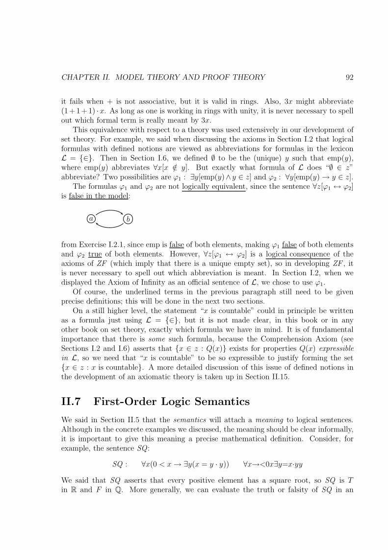
CHAPTER II. MODEL THEORY AND PROOF THEORY 92
it fails when + is not associative, but it is valid in rings. Also, 3x might abbreviate(1 + 1 + 1) ·x. As long as one is working in rings with unity, it is never necessary to spellout which formal term is really meant by 3x.
This equivalence with respect to a theory was used extensively in our development ofset theory. For example, we said when discussing the axioms in Section I.2 that logicalformulas with defined notions are viewed as abbreviations for formulas in the lexiconL = {∈}. Then in Section I.6, we defined ∅ to be the (unique) y such that emp(y),where emp(y) abbreviates ∀x[x /∈ y]. But exactly what formula of L does “∅ ∈ z”abbreviate? Two possibilities are ϕ1 : ∃y[emp(y)∧ y ∈ z] and ϕ2 : ∀y[emp(y)→ y ∈ z].
The formulas ϕ1 and ϕ2 are not logically equivalent, since the sentence ∀z[ϕ1 ↔ ϕ2]is false in the model:
a b
from Exercise I.2.1, since emp is false of both elements, making ϕ1 false of both elementsand ϕ2 true of both elements. However, ∀z[ϕ1 ↔ ϕ2] is a logical consequence of theaxioms of ZF (which imply that there is a unique empty set), so in developing ZF , itis never necessary to spell out which abbreviation is meant. In Section I.2, when wedisplayed the Axiom of Infinity as an official sentence of L, we chose to use ϕ1.
Of course, the underlined terms in the previous paragraph still need to be givenprecise definitions; this will be done in the next two sections.
On a still higher level, the statement “x is countable” could in principle be writtenas a formula just using L = {∈}, but it is not made clear, in this book or in anyother book on set theory, exactly which formula we have in mind. It is of fundamentalimportance that there is some such formula, because the Comprehension Axiom (seeSections I.2 and I.6) asserts that {x ∈ z : Q(x)} exists for properties Q(x) expressiblein L, so we need that “x is countable” to be so expressible to justify forming the set{x ∈ z : x is countable}. A more detailed discussion of this issue of defined notions inthe development of an axiomatic theory is taken up in Section II.15.
II.7 First-Order Logic Semantics
We said in Section II.5 that the semantics will attach a meaning to logical sentences.Although in the concrete examples we discussed, the meaning should be clear informally,it is important to give this meaning a precise mathematical definition. Consider, forexample, the sentence SQ :
SQ : ∀x(0 < x→ ∃y(x = y · y)) ∀x→<0x∃y=x·yy
We said that SQ asserts that every positive element has a square root, so SQ is Tin R and F in Q. More generally, we can evaluate the truth or falsity of SQ in an
CHAPTER II. MODEL THEORY AND PROOF THEORY 93
arbitrary abstract structure A. This structure should consist of a domain of discourseA (a non-empty set over which the variables “range”), together with a binary productoperation ·A, a binary relation <A, and a distinguished element 0A. We shall writeA = (A; ·A, <A, 0A). We are following here the usual convention in model theory ofusing italic letters, A,B,C,D, · · · for the domain of discourse of a structure and thecorresponding gothic or fraktur letters, A,B,C,D, · · · for the full structure. To be reallyformal, this subscripted notation (·A, <A, 0A) indicates the presence of a function whichassigns to symbols of L a semantic entity of the correct type:
Definition II.7.1 Given a lexicon for predicate logic, L = F ∪P =⋃n∈ω Fn ∪
⋃n∈ω Pn
(see Definitions II.5.2 and II.5.3 ), a structure for L is a pair A = (A, I) such that A isa non-empty set and I is a function with domain L with each I(s) a semantic entity ofthe correct type; specifically, writing sA for I(s):
☞ If f ∈ Fn with n > 0, then fA : An → A.
☞ If p ∈ Pn with n > 0, then pA ⊆ An.
☞ If c ∈ F0, then cA ∈ A.
☞ If p ∈ P0, then pA ∈ 2 = {0, 1} = {F, T}.
Note the special case for n = 0. Symbols in F0 are constant symbols, so they donotean element of the universe of the structure. Symbols in P0 are proposition letters, sothey denote a truth value, F or T ; for these, the universe of the structure is irrelevant.We follow the usual convention of using 0 to denote “false” and 1 to denote “true”.
We are also following the usual convention in model theory of requiring A 6= ∅, sinceallowing the empty structure leads to some pathologies later (see Remark II.8.16).
Unless there is danger of confusion, we shall be fairly informal in denoting structures.For example, if L = {p, f} with p ∈ P2 and f ∈ F1, we might say, “let A = (R;<, cos)”,since this makes it clear that pA is the < relation and fA is the cosine function. But ifL = F1 = {f, g}, the definition, “let A = (R; sin, cos)” might be ambiguous, and we needto say, e.g., that fA is the cosine function and gA is the sine function. If L = {+, ·, 0, 1},we might simply say, “let A = R”, since it is usually clear from context that the symbols+, ·, 0, 1 denote the expected addition, multiplication, zero, and one in the real numbers.We are perpetuating here the standard abuse of notation employed in algebra, wherethe same symbols +, · are used to denote the addition and multiplication functions ofsome (any) ring, as well as to denote symbols in formal expressions such as the term(polynomial) x · y + z + 1.
We shall rarely use the “(A, I)” terminology from Definition II.7.1. We gave it mainlyto make it clear what A is set-theoretically; it is also useful in discussing reducts andexpansions (see Definition II.8.14).
We shall next define the notion “A |= ϕ” (ϕ is true in A), where A is a structurefor L and ϕ is a sentence of L. Roughly, this is done by recursion on ϕ. Consider, forexample, the above sentence SQ , where L = {<, 0, ·}, and A = Q (with the usual order,

CHAPTER II. MODEL THEORY AND PROOF THEORY 94
zero, and product understood). That this is false in A will be expressed symbolically inone of the following three equivalent ways:
1. A 6|= SQ 2. A |= ¬SQ 3. valA(SQ) = F
The double turnstile symbol “|=” here is usually read “models” or “satisfies”. Forms (1)and (2) are the more standard terminologies, but we use (3) to emphasize that given A,we are defining a function valA on the sentences of L. Our precise defnition of valA(SQ)will unwind the syntax of SQ ; it begins with a ∀x; informally, the statement isn’t truefor all x ∈ Q, for example,
valA(0 < x→ ∃y(x = y · y)
)[2] = F . (A)
Since the formula 0 < x→ ∃y(x = y ·y) is not a sentence, but has x as a free variable, the“[2]” is needed to say that we are interpreting the x as the rational number 2, whereas
valA(0 < x→ ∃y(x = y · y)
)[4] = T . (B)
The reason for (A) is that 2 is positive but does not have a square root in Q; formally:
valA(0 < x
)[2] = T , (C)
butvalA
(∃y(x = y · y)
)[2] = F , (D)
so that (A) follows by the usual truth table for → (i.e., (T → F ) = F ). We explain(C) and (D) by using, respectively, the meaning of <A and the meaning of ∃. If we usethe official Polish notation, then the way we (recursively) compute the value of valA(ϕ)is determined by the first (leftmost) symbol of ϕ. Because of this, we present the officialdefinition of val (Definitions II.7.4, II.7.6, II.7.8) using the official Polish notation.
Before giving a precise definition, one more remark on the “[2]” terminology: Thisnotation easily extends to formulas with several free variables, but there is a danger ofambiguity. For example, with A = Q, the meaning of valA(y = x · z)[2, 6, 3] is not clear,since it does not specify which of y, x, z get replaced by which of 2, 6, 3. In most cases,this is clear from context (one is either ordering the variables alphabetically or by theirorder of occurrence in the formula), but when it is not, we shall use the notation:
valA(y = x · z
) [x y z2 6 3
]= T valA
(y = x · z
) [y x z2 6 3
]= F .
The array notationh
x y z2 6 3
i
really denotes a function σ whose domain is the set of variablesymbols {x, y, z}, and σ(x) = 2, σ(y) = 6, σ(z) = 3. So, we need to define valA(ϕ)[σ]; fora fixed A, this is a function of ϕ and σ, and will take values in 2 = {0, 1} = {F, T}. Itwill be defined by recursion on ϕ. Now, to compute valA(y = x · z)[σ], we need to usethe function ·A to compute valA(x · z) ∈ A and see if that is the same as σ(y). Moregenerally, before defining the truth value of formulas, we need to define valAτ [σ] ∈ A forterms τ .
CHAPTER II. MODEL THEORY AND PROOF THEORY 95
Definition II.7.2 For terms τ , let V (τ) be the set of variables which occur in τ . Forformulas ϕ, let V (ϕ) be the set of variables which have a free occurrence in ϕ.
Definition II.7.3 If α is either a term or a formula, an assignment for α in A is afunction σ such that V (α) ⊆ dom(σ) ⊆ VAR and ran(σ) ⊆ A.
Definition II.7.4 If A is a structure for L, then we define valA(τ)[σ] ∈ A whenever τis a term of L and σ is an assignment for τ in A as follows:
1. valA(x)[σ] = σ(x) when x ∈ dom(σ).
2. valA(c)[σ] = cA when c ∈ F0.
3. valA(fτ1 · · · τn)[σ] = fA(valA(τ1)[σ], . . . , valA(τn)[σ]) when f ∈ Fn and n > 0.
If V (τ) = ∅, then valA(τ) abbreviates valA(τ)[σ].
Again, with A = Q:
valA(x · y
) [x y2 6
]= valA
(x) [x y2 6
]·A valA
(y) [x y2 6
]= 2 ·A 6 = 12 .
We are using successively clauses (3) and (1) of the definition and the meaning of ·A. Notethat in the definition of “assignment”, we are allowing dom(σ) to be a proper supersetof V (α); otherwise clauses such as (3) would be rather awkward to state. However, oneeasily verifies by induction:
Exercise II.7.5 valA(τ)[σ] only depends on σ↾V (τ); that is, if σ′↾V (τ) = σ↾V (τ) thenvalA(τ)[σ′] = valA(τ)[σ].
In particular, when V (σ) = ∅, the notation valA(τ) for valA(τ)[σ] is unambiguous.Definition II.7.4 was by recursion on the length of terms, while the definition of the
truth value for an atomic formula is explicit:
Definition II.7.6 If A is a structure for L, then we define valA(ϕ)[σ] ∈ {0, 1} = {F, T}whenever ϕ is an atomic formula of L and σ is an assignment for ϕ in A as follows:
1. valA(p)[σ] = pA when p ∈ P0.
2. valA(pτ1 · · · τn)[σ] = T iff (valA(τ1)[σ], . . . , valA(τn)[σ]) ∈ pA when p ∈ Pn andn > 0.
3. valA(=τ1τ2)[σ] = T iff valA(τ1)[σ] = valA(τ2)[σ].
Note that clause (3) is needed because = is a logical symbol, not a symbol L, and A
does not assign a meaning to =; rather, τ1 = τ2 always means that τ1, τ2 are the sameobject.
The following definition will be useful when defining the value of formulas:
CHAPTER II. MODEL THEORY AND PROOF THEORY 96
Definition II.7.7 σ + (y/a) = σ↾(VAR\{y}) ∪ {(y, a)}.
That is, we assign y value a, if necessary discarding the value σ gives to y. For example,[x4
]+ (y/2) =
[x y4 2
] [x y z4 5 6
]+ (y/2) =
[x y z4 2 6
].
The truth value of a formula ϕ is, like the value of a term, computed recursively:
Definition II.7.8 If A is a structure for L, then we define valA(ϕ)[σ] ∈ {0, 1} = {F, T}whenever ϕ is a formula of L and σ is an assignment for ϕ in A as follows:
1. valA(¬ϕ)[σ] = 1− valA(ϕ)[σ].
2. valA(∧ϕψ)[σ], valA(∨ϕψ)[σ], valA(→ϕψ)[σ], and valA(↔ϕψ)[σ], are obtained fromvalA(ϕ)[σ] and valA(ψ)[σ] using the truth tables (Table 1, page 4 ) for ∧,∨,→,↔.
3. valA(∃yϕ)[σ] = T iff valA(ϕ)[σ + (y/a)] = T for some a ∈ A.
4. valA(∀yϕ)[σ] = T iff valA(ϕ)[σ + (y/a)] = T for all a ∈ A.
A |= ϕ[σ] means valA(ϕ)[σ] = T . If V (ϕ) = ∅ (that is, ϕ is a sentence), then valA(ϕ)abbreviates valA(ϕ)[σ], and A |= ϕ means valA(ϕ) = T .
Of course, clause (1) is equivalent to saying that we are using the usual truth table for¬. Definition II.7.7 is needed because σ may give values to variables which are not freein ϕ; then those values are irrelevant, and they may need to be discarded in computingthe truth value of ϕ. For example, in the rationals:
valA(∃y(x = y · y)
) [x y z4 5 6
]= T because valA
(x = y · y
) [x y z4 2 6
]= T .
As with terms, one easily verifies by induction:
Exercise II.7.9 valA(ϕ)[σ] only depends on σ↾V (ϕ); that is, if σ′↾V (ϕ) = σ↾V (ϕ) thenvalA(ϕ)[σ′] = valA(ϕ)[σ].
In particular, when ϕ is a sentence, the notation valA(ϕ) for valA(ϕ)[σ] is unambiguous.We now describe some related semantic notions and then state the two main model
theory results to be proved in this chapter.
Definition II.7.10 If A is a structure for L and Σ is a set of sentences of L, thenA |= Σ iff A |= ϕ for each ϕ ∈ Σ.
The symbols “A |= ϕ” are usually read “A satisfies Σ” or “A is a model for Σ”. Forexample, as we said in Section 0.4, a group is a model for the axioms GP of group theory.
Definition II.7.11 If Σ is a set of sentences of L and ψ is a sentence of L, then Σ |= ψholds iff A |= ψ for all L-structures A such that A |= Σ.
CHAPTER II. MODEL THEORY AND PROOF THEORY 97
In English, we say that ψ is a semantic consequence or logical consequence of Σ. Notethe overloading of the symbol |=; it has been given two different meanings in DefinitionsII.7.10 and II.7.12. This never causes an ambiguity because it is always clear from contextwhether the object on the left side of the |= (A or Σ) is a structure or a set of sentences.In all its uses, the double turnstile |= always refers to semantic notions, whereas thesingle turnstile ⊢ refers to the syntactic notion of provability; Σ ⊢ ψ means that thereis a formal proof of ψ from Σ (to be defined in Section II.10). By the CompletenessTheorem (Theorem II.12.1), Σ ⊢ ψ iff Σ |= ψ.
Definition II.7.12 If Σ is a set of sentences of L then Σ is semantically consistent(Con|=(Σ) )iff there is some A such that A |= Σ. “inconsistent” means “not consistent”.
There is also a syntactic notion Con⊢(Σ), which asserts that Σ cannot prove a con-tradiction in the formal proof theory (see Section II.10). The Completeness Theoremwill also imply that Con⊢(Σ) iff Con|=(Σ). After that, we drop the subscripts and justwrite Con(Σ).
The usual axiomatic theories discussed in algebra texts (e.g., groups, rings, andfields) are clearly consistent, since these axiom sets are usually presented together withsample models of them. It is easy to write down “artificial” examples of inconsistent setsof sentences, but the notion of inconsistency occurs naturally in the following lemma,whose proof is immediate from the definition of |=:
Lemma II.7.13 (reductio ad absurdum) If Σ is a set of sentences of L and ψ is asentence of L, then
a. Σ |= ψ iff Σ ∪ {¬ψ} is semantically inconsistent.
b. Σ |= ¬ψ iff Σ ∪ {ψ} is semantically inconsistent.
The proof theory version of this is also true (see Lemma II.11.4), and correspondsto a common step in informal mathematical reasoning: To prove ψ, we reduce ¬ψ to anabsurdity; that is, we assume that ψ is false and derive a contradiction. The use of Latinin phrases such as “reductio ad absurdum” and “modus ponens” (see Definition II.10.3)originates with the Scholastic philosophers in the Middle Ages, although the conceptsinvolved go back to Aristotle.
Theorem II.7.14 (Compactness Theorem) If Σ is a set of sentences of L:
1. If every finite subset of Σ is semantically consistent, then Σ is semantically con-sistent.
2. If Σ |= ψ, then there is a finite ∆ ⊆ Σ such that ∆ |= ψ.

CHAPTER II. MODEL THEORY AND PROOF THEORY 98
In view of Lemma II.7.13, (1) and (2) are equivalent statements. We shall prove themin Section II.12.
The Compactness Theorem involves only |=, so it is a theorem of “pure model the-ory”, whereas the Completeness Theorem is a result which relates model theory (|=) toproof theory (⊢). We shall actually prove the Completeness Theorem first (see TheoremII.12.1). From this, Compactness is easy, since if one replaces |= by ⊢ in (2), the resultwill follow from the fact that formal proofs are finite.
The Lowenheim-Skolem Theorem is another result of “pure model theory” involvingthe cardinalities of models.
Definition II.7.15 If A is a structure for L with universe A, then |A| denotes |A|.
Likewise, other statements about the size of A really refer to |A|; for example “A isan infinite model” means that |A| is infinite.
Theorem II.7.16 (Lowenheim–Skolem Theorem) Let Σ be a set of sentences of Lsuch that for all finite n, Σ has a (finite or infinite) model of size ≥ n. Then for allκ ≥ max(|L|,ℵ0), Σ has a model of size κ.
Here, |L| means literally the number of nonlogical symbols. In all examples up tonow, this has been finite. As long as |L| ≤ ℵ0, this theorem says, informally, that first-order logic cannot distinguish between infinite cardinalities, since if Σ has an infinitemodel, it has models of all infinite sizes.
If L is uncountable, then we really do need κ ≥ |L| for the theorem to hold. Forexample, suppose L = F0 = {cα : α < λ}, where λ is an infinite cardinal, and Σ ={cα 6= cβ : α < β < κ}. Then Σ has a model of size κ iff κ ≥ λ. This example mayseem a bit artificial, but uncountable languages are useful in model theory; for example,they occur in the proof of the Lowenheim–Skolem Theorem in Section II.12; this proofwill occur after our proof of the Compactness Theorem provides us with a technique forconstructing a model of a desired cardinality.
Note that finite sizes are special. For example, if Σ consists of the one sentence∀x, y, z(x = y ∨ y = z ∨ z = x), then Σ has models of sizes 1 and 2, but no other sizes.
II.8 Further Semantic Notions
We collect here a few auxilliary semantic notions.
Definition II.8.1 If ψ is a formula of L, then ψ is logically valid iff A |= ψ[σ] for allL-structures A and all assignments σ for ψ in A.
A sentence ψ is logically valid iff ∅ |= ψ, where ∅ is the empty set of sentences, sinceDefinition II.7.10 implies that A |= ∅ for all A. The formula x = x and the sentence

CHAPTER II. MODEL THEORY AND PROOF THEORY 99
∀x(x = x) are logically valid because our definition of |= always interprets the logicalsymbol = as true identity. Many formulas, such as ∀xp(x) → ¬∃x¬p(x), are obviouslylogically valid, and many others, such as p(x)→ ∀yp(y), are obviously not logically valid.There are many such trivial examples, but by a famous theorem of Church (see ChapterIII), there is no algorithm which can decide in general which formulas are logicallyvalid. A subset of the logically valid formulas, the propositional tautologies (such asp(x)→ ¬¬p(x) ), is decidable (using truth tables); see Section II.9.
Definition II.8.2 If ϕ, ψ are formulas of L, then ϕ, ψ are logically equivalent iff theformula ϕ↔ ψ is logically valid.
This is the same as saying that A |= ϕ[σ] iff A |= ψ[σ] for all A and all σ. Forexample, p(x) ∨ q(x) and q(x) ∨ p(x) are logically equivalent. All universal closures of aformula (see Definition II.5.6) are logically equivalent:
Lemma II.8.3 If ϕ is a formula, and the sentences ψ and χ are both universal closuresof ϕ, then ψ, χ are logically equivalent.
Proof. Say y1, . . . , yk are the free variables of ϕ, where k ≥ 0. Then ψ is of the form∀x1∀x2 · · · ∀xnϕ, where each yi is listed at least once in x1, x2, . . . , xn. Note that A |= ψiff A |= ϕ[a1, . . . , ak] for all a1, . . . , ak ∈ A. Since the same is also true for χ, we haveA |= ψ iff A |= χ. �
In particular, if ϕ is a sentence, then it is a universal closure of itself and all universalclosures of ϕ are logically equivalent to ϕ. In view of Lemma II.8.3, if ϕ is any formula,we shall usually say “the universal closure of ϕ” to refer to some (any) universial closureof ϕ, since it usually will not matter which one we use.
There is also a relative notion of logical equivalence:
Definition II.8.4 If ϕ, ψ are formulas of L and Σ is a set of sentences of L, then ϕ, ψare equivalent with respect to Σ iff the universal closure of ϕ↔ ψ is true in all modelsof Σ. If τ1 and τ2 are terms, then τ1, τ2 are equivalent with respect to Σ iff for all A |= Σand all assignments σ for τ1, τ2 in A, valA(τ1)[σ] = valA(τ2)[σ].
This notion came up in the discussion of abbreviations (see Section II.6). For example,if Σ contains the associative law, then the terms x · (y · z) and (x · y) · z are equivalentwith respect to Σ, so as long as we are discussing only models of Σ, it is safe to use xyzas an abbreviation, without having to remember which of these two terms it abbreviates.One could define τ1, τ2 to be logically equivalent iff they are equivalent with respect to∅, but this is uninteresting by:
Exercise II.8.5 If valA(τ1)[σ] = valA(τ2)[σ] for all A and σ, then τ1 and τ2 are the sameterm.

CHAPTER II. MODEL THEORY AND PROOF THEORY 100
We now consider the notion of substitution:
Definition II.8.6 If β and τ are terms and x is a variable, then β(x τ) is the termwhich results from β by replacing all free occurrences of x by τ .
Of course, one must verify that β(x τ) really is a term, but this is easily done byinduction on β.
For example, using the language of ordered rings LOR = {<,+, ·,−, 0, 1} as in SectionII.5, if β is the term (polynomial) x ·y then β(x x+z) is (x+z) ·y. The parentheses areneeded here, but in the official Polish, where β is ·xy, one literally replaces x by +xz tosee that β(x x+z) is ·+xzy. This substitution does the “right thing” in the semantics,when we compute the value of terms as in Section II.7. In the rationals,
valA(β(x x + z)
) [x y z1 2 5
]= valA
(β) [x y z6 2 5
]= 12 .
In the second expression, we changed the value of x to 6 = valA(x + z)[1, 5]. Moregenerally, to evaluate β(x τ) given an assignment σ, we change the value of σ(x) tovalA(τ)[σ], and then evaluate β. Using the terminology of Definition II.7.7,
Lemma II.8.7 If A is a structure for L, and σ is both an assignment for β in A andan assignment for τ in A (see Definition II.7.3 ), and a = valA(τ)[σ], then
valA(β(x τ))[σ] = valA(β)[σ + (x/a)] .
Proof. Induct on β. �
There is a similar discussion for formulas:
Definition II.8.8 If ϕ is a formula, x is a variable, and τ is a term, then ϕ(x τ) isthe formula which results from ϕ by replacing all free occurrences of x by τ .
Of course, one must verify that ϕ(x τ) really is a formula, but this is easily doneby induction on ϕ.
Roughly, ϕ(x τ) says about τ what ϕ says about x. For example, again using LOR,if ϕ is the formula ∃y(y · y = x + z), asserting “x + z has a square root”, then ϕ(x 1)is ∃y(y · y = 1 + z) asserting “1 + z has a square root”. But ϕ(y 1) is ϕ; since y is onlya bound (dummy) variable, ϕ doesn’t say anything about y.
One must use some care when τ contains variables. For example, let ϕ be ∃y(x < y).Then ∀xϕ is true in R, so one would expect the univeral closure of each ϕ(x τ) to betrue. For example, if τ is, respectively, 1 and z + z, then ∃y(1 < y) and ∀z∃y(z + z < y)are both true in R. However, if τ is y + 1, then ϕ(x τ) is the sentence ∃y(y + 1 < y),which is false in R. The problem is that the variable y in τ got “captured” by the ∃y,changing its meaning. To make this problem precise,

CHAPTER II. MODEL THEORY AND PROOF THEORY 101
Definition II.8.9 A term τ is free for x in a formula ϕ iff no free occurrence of x isinside the scope of a quantifier ∃y or ∀y where y is a variable which occurs in τ .
If the substitution is free, then it has the intended meaning, made formal by:
Lemma II.8.10 Assume that A is a structure for L, ϕ is a formula of L, τ is a term ofL, and σ is both an assignment for ϕ in A and an assignment for τ in A (see DefinitionII.7.3 ), and a = valA(τ)[σ]. Assume that τ is free for x in ϕ. Then
A |= ϕ(x τ)[σ] iff A |= ϕ[σ + (x/a)] .
Proof. Induct on ϕ. The basis, where ϕ is atomic, uses Lemma II.8.7. Also note thatif x is not free in ϕ, then ϕ(x τ) is ϕ, and the value assigned by σ to x is irrelevant,so the lemma in this case is immediate and does not use the inductive hypothesis. Thepropositional cases for the induction are straightforward. Now, consider the the quantifierstep, where ϕ is ∃yψ or ∀yψ. Assume that x really has a free occurrence in ϕ (otherwisethe result is immediate). Then the variables y and x must be distinct, and x has a freeoccurrence in ψ, so that y cannot occur in τ (since τ is free x in ϕ). The induction is nowstraightforward, using the definition of |= (see Definition II.7.8). This definition requiresthat we consider various σ+(y/b), and we observe that a = valA(τ)[σ] = valA(τ)[σ+(y/b)]because y does not occur in τ . �
We frequently use the following simpler notation for substitution:
Notation II.8.11 ϕ(τ) abbreviates ϕ(x τ) when it is clear from context that it is thevariable x which is being replaced. To that end, one often refers to ϕ as “ϕ(x)” duringthe discussion. Likewise if one refers to ϕ as “ϕ(x1, . . . , xn)”, and τ1, . . . , τn are terms,then ϕ(τ1, . . . , τn) denotes the formula obtained by simultaneously replacing each freeoccurrence of xi in ϕ by τi.
As an example using this convention, we mention that Lemma II.8.10 implies:
Corollary II.8.12 If τ is free for x in ϕ(x), then the formulas ∀xϕ(x) → ϕ(τ) andϕ(τ)→ ∃xϕ(x) are logically valid.
Proof. By Lemma II.8.10 and the definitions (II.8.1 and II.7.8) of “logically valid” and“|=”. �
For another example, say we are talking about the real numbers, using the lexiconL = {+, ·,−, 0, 1}, and we say, “let ϕ(x, y) be x + 1 = y”. Then ϕ(1 + 1, 1 + (1 + 1)) is(1 + 1) + 1 = 1 + (1 + 1), which is true in R, while ϕ(1 + (1 + 1), 1 + 1) is false in R. Thestructure A here is (R; +, ·,−, 0, 1). Note that the two statements, A |= ϕ(1+1, 1+(1+1))and A |= ϕ[2, 3] say essentially the same thing, but are formally different. The first saysthat the sentence ϕ(1+1, 1+(1+1)) is true in A, while the second says that the formulax+ 1 = y is true in A if we assign x value 2 and y value 3. The fact that these have thesame meaning generalizes to:

CHAPTER II. MODEL THEORY AND PROOF THEORY 102
Lemma II.8.13 Assume that A is a structure for L, ϕ(x1, . . . , xn) is a formula of Lwith no variables other than x1, . . . , xn free. and τ1, . . . , τn are terms of L with no freevariables. Let ai = valA(τi). Then A |= ϕ(τ1, . . . , τn) iff A |= ϕ[a1, . . . , an].
Proof.
A |= ϕ(τ1, τ2, . . . , τn) iff A |= ϕ(x1, τ2, . . . , τn)[a1] iff A |= ϕ(x1, x2, . . . , τn)[a1, a2]
iff · · · · · · iff A |= ϕ(x1, x2, . . . , xn)[a1, . . . , an] .
Each of the n ‘iff’s uses Lemma II.8.10. �
So far, the lexicon L has been fixed for each structure under discussion. But onefrequently considers a fixed domain of discourse and varies the language. For example,we may consider the real numbers as a field, A = (R; +, ·,−, 0, 1), so that our language isL1 = {+, ·,−, 0, 1}. But we may also wish to consider R just as an abelian group, usingL0 = {+,−, 0}, and write A↾L0 = (R; +,−, 0). Then we say that A↾L0 is a reduct of A,and that A is an expansion of A↾L0. In the terminology of category theory, we wouldsay that we are describing forgetful functor from the category of fields to the categoryof abelian groups, since in the group A↾L0, we forget about the product operation.
The terminology L0 ⊆ L1 implies that all the symbols have the same types in L0 andL1; we never, in one discussion, use the same name for symbols of different types. We givethe general definition of reduct and expansion following the terminology of DefinitionII.7.1:
Definition II.8.14 If L0 ⊆ L1 and A = (A, I) is a structure for L1 then A↾L0 denotes(A, I↾L0). A↾L0 is called a reduct of A and A is called an expansion of A↾L0.
Note that in Definition II.7.1, I was really a function with domain L1, and we are literallyrestricting this function to L0.
Often, we start with an L0 structure and ask about its expansions. For example, if(A; +,−, 0) is an abelian group, we might ask when it is the additive group of a field.This is really a (fairly easy) algebra question; using our model-theoretic terminolgy,we are asking whether (A; +,−, 0) has an expansion of the form (A; +, ·,−, 0, 1) whichsatisfies the field axioms.
The next lemma shows that notions such as Σ |= ψ (Definition II.7.11) and Con|=(Σ)(Definition II.7.12) do not change if we expand the language. Thus, we did not mentionL explicitly and write something like A |=L ψ or Con|=,L(Σ).
Lemma II.8.15 Suppose that Σ is a set of sentences of L0 and ψ is a sentence of L0
and suppose that L0 ⊆ L1. Then the following are equivalent:
α. A0 |= ψ for all L0-structures A0 such that A0 |= Σ.
β. A1 |= ψ for all L1-structures A1 such that A1 |= Σ.

CHAPTER II. MODEL THEORY AND PROOF THEORY 103
Also, the following are equivalent:
a. There is an L0-structure A0 such that A0 |= Σ.
b. There is an L1-structure A1 such that A1 |= Σ.
Proof. For (b) → (a): If A1 |= Σ then also A1↾L0 |= Σ, since the truth of L0 sentencesis the same in A1 and A1↾L0.
For (a)→ (b): Let A0 be any L0-structure such that A0 |= Σ. Expand A0 arbitrarilyto an L1-structure A1. Then we still have A1 |= Σ.
(α)↔ (β) is similar. �
Remark II.8.16 The above proof is essentially trivial, but it does rely on the fact thatstructures are non-empty by Definition II.7.1. If we allowed the domain of discourse Ato be empty, then all the basic definitions could still be made, but this lemma wouldfail. For example, if ψ is ∀xp(x) → ∃xp(x), then ψ is false in the empty set (where∀xp(x) is true and ∃xp(x) is false), but ψ is true in every other structure. If L0 = {p}and L1 = {p, c} with c a constant symbol, we would have the somewhat pathologicalsituation that {¬ψ} would be consistent as an L0-sentence but not as an L1-sentence.In the proof of (a) → (b), there would be no way to expand the empty structure to anL1-structure because constant symbols must be interpreted as elements of A. This sortof pathology explains why the universe is always assumed to be non-empty in modeltheory.
In reduct/expansion, we fix A and decrease/increase L. This should not be con-fused with submodel/extension, where we fix L and decrease/increase A. The notion ofsubmodel generalizes the notions of subgroup, subring, etc., from algebra:
Definition II.8.17 Suppose that A = (A, I) and B = (B,J ) are structures for L. ThenA ⊆ B means that A ⊆ B and the functions and predicates of A are the restrictions ofthe corresponding functions and predicates of B. Specifically:
☞ If f ∈ Fn with n > 0, then fA = fB↾An.
☞ If p ∈ Pn with n > 0, then pA = pB∩ An.
☞ If c ∈ F0, then cA = cB.
☞ If p ∈ P0, then pA = pB ∈ 2 = {0, 1} = {F, T}.
A is called a submodel of B and B is called an extension of A.
In the case of constants and functions, observe that cA must be an element of A andfA must map into A. So, if we start with B and an arbitrary non-empty A ⊆ B, it isnot true in general that A can be made into a submodel of B. For example, supposeB = (B; ·, i, 1} is a group, where, as in Section II.5, we are taking the language of grouptheory to be L = {·, i, 1}. If A ⊆ B, it cannot be made into a submodel of B unless it

CHAPTER II. MODEL THEORY AND PROOF THEORY 104
is closed under product and inverse and contains 1, that is, unless it is a subgroup. Alsonote that which subsets form submodels changes if we go to reducts or expansions. Forexample, if we reduct to the language L0 = {·}, we can still express the group axioms (asin Section 0.4), but submodels of (B; ·) are subsemigroups; that is, closed under productbut not necessarily inverse.
There is a notion of isomorphism between groups or rings; this generalizes easily toarbitrary structures.
Definition II.8.18 Suppose that A = (A, I) and B = (B,J ) are structures for thesame language L. Φ is an isomorphism from A onto B iff Φ : A −→1−1
onto B and Φ preservesthe structure. Specifically:
☞ If f ∈ Fn with n > 0, then fB(Φ(a1), . . . ,Φ(an)) = Φ(fA(a1, . . . , an)).
☞ If p ∈ Pn with n > 0, then (Φ(a1), . . . ,Φ(an)) ∈ pB iff (a1, . . . , an) ∈ pA.
☞ If c ∈ F0, then cB = Φ(cA).
☞ If p ∈ P0, then pB = pA ∈ 2 = {0, 1} = {F, T}.
A and B are isomorphic ( A ∼= B ) iff there exists an isomorphism from A onto B.
This definition also generalizes Definition I.7.14, which was given for the special caseof ordered structures.
A set of axioms Σ is complete iff it decides all possible statements:
Definition II.8.19 If Σ is a set of sentences of L, then Σ is complete (with respectto L ) iff Σ is semantically consistent and for all sentences ϕ of L, either Σ |= ϕ orΣ |= ¬ϕ.
If we just say “Σ is complete”, it is understood that L is the set of symbols actuallyused in Σ. Σ will usually not be complete with respect to a larger L:
Exercise II.8.20 Suppose that Σ is a set of sentences of L and L′ % L, with L′\Lcontaining at least one predicate symbol. Then Σ cannot be complete with respect to L′.
Hint. Consider ϕ of the form ∃x1, . . . , xn p(x1, . . . , xn). �
A (perhaps artificial) example of a complete Σ is the theory of a given structure.
Definition II.8.21 If A is a structure for L, then the theory of A, Th(A) is the set ofall L-sentences ϕ such that A |= ϕ.
Lemma II.8.22 Th(A) is complete (with respect to L ).

CHAPTER II. MODEL THEORY AND PROOF THEORY 105
Proof. Th(A) is semantically consistent because A |= Th(A), and for all sentences ϕ ofL, either ϕ ∈ Σ or (¬ϕ) ∈ Σ. �
There are many natural examples of complete theories in algebra. We shall describea few in Section II.13. Further examples may be found in model theory texts, such as[5, 24].
The following example from algebra illustrates one additional point about formalizingalgebraic theories.
Example II.8.23 Let L = {0, 1,+, ·,−, i}, where “−” denotes the unary additive in-verse and “i” denotes the unary multiplicative inverse (or reciprocal). Let Σ in L be theaxioms for fields, expressed by:
1. The axioms for groups, written in +, 0,− (see γ1, γ2,1, γ2,2 in Section II.5).
2. The associative and identity laws, written in ·, 1 (see γ1, γ2,1 in Section II.5).
3. The commutative laws: ∀x, y [x · y = y · x] and ∀x, y [x+ y = y + x].
4. The distributive law: ∀x, y, z [x · (y + z) = (x · y) + (x · z)].5. The multiplicative inverse law: ∀x [x 6= 0→ x · i(x) = 1]].
6. i(0) = 0.
7. 0 6= 1.
Axiom (5) states the existence of a reciprocal for every non-zero element. Informally,in algebra, we say “1/0 is undefined”. Formally, since our model theory does not allowfor partially defined function symbols, i(x) is defined for all x, and we just assert thatit denotes the reciprocal of x when the reciprocal exists (i.e., when x 6= 0). The valueof i(0) is “irrelevant”, but we include axiom (6) specifying its value so that the usualnotion of field isomorphism in algebra corresponds to the notion of isomorphism in modeltheory, where Definition II.8.18 requires Φ(iA(0A)) = iB(0B). If we dropped axiom (6),then there would be three non-isomorphic fields of order three; depending on whetheri(0) is 0, 1, or 2. Axiom (7) disallows the “trivial” 1-element field.
II.9 Tautologies
Informally, a propositional tautology (or, just tautology) is a formula whose logical validityis apparant just from the meaning of the propositional connectives, without referenceto the meaning of =, ∀, ∃. For example, p(x) → p(x) is a tautology, whereas ∀xp(x) →∀yp(y) and x = x are not, since you have to understand the meaning of ∀ and =,respectively, to see that they are logically valid.
Definition II.9.1 A formula is basic iff (in its Polish notation) it does not begin witha propositional connective.

CHAPTER II. MODEL THEORY AND PROOF THEORY 106
For example, ∀xp(x)→ ∀yp(y) (i.e. →∀xpx∀ypy) is not basic, but it is an implicationbetween the two basic formulas ∀xpx and ∀ypy. In the definition of “tautology”, weconsider these basic formulas as distinct un-analyzed atoms. Note that every formula isobtained from basic formulas by using propositional connectives.
Definition II.9.2 A truth assignment for L is a function v from the set of basic for-mulas of L into {0, 1} = {F, T}. Given such a v, we define (recursively) v(ϕ) ∈ {F, T}as follows:
1. v(¬ϕ) = 1− v(ϕ).
2. v(∧ϕψ), v(∨ϕψ), v(→ϕψ), and v(↔ϕψ), are obtained from v(ϕ) and v(ψ) usingthe truth tables (Table 1, page 4 ) for ∧,∨,→,↔.
ϕ is a propositional tautology iff v(ϕ) = T for all truth assignments v.
There is a similarity between this definition and Definition II.7.8 (of |=), but herewe are only studying the meaning of the propositional connectives. To test whether ϕis a tautology, you just check all possible assignments of T or F to the basic formulasout of which ϕ is built. For example, if ϕ is ∀xp(x) → ∀yp(y), then one such v hasv(∀xp(x)) = T and v(∀yp(y)) = F ; this is allowed because ∀xp(x) and ∀yp(y) aredistinct formulas (even though they are logically equivalent); this v makes v(ϕ) = F , sothat ϕ is not a tautology. However, p(x) → p(x) is built out of the one basic formulap(x), which v may make either T or F , but in either case v(p(x) → p(x)) = T , so thatp(x)→ p(x) is a tautology.
Comparing Definitions II.9.2 and II.7.8 and the definition (II.8.1) of logical validity,we see:
Exercise II.9.3 Every propositional tautology is logically valid.
II.10 Formal Proofs
We now give a presentation of formal proof theory, as we promised in Sections 0.4 andII.2. As mentioned in Section II.2, we are striving for a system which is easy to defineand analyze mathematically, not one which is easy to use in a practical settings. Someremarks about “practical” proof theories and references to the literature are in SectionII.17.
In this proof theory, we have one rule of inference:
MODUS PONENS:ϕ ϕ→ ψ
ψ
Informally, this means that if we have proved both ϕ and ϕ→ ψ, then we can concludeψ. Formally, Modus Ponens is embedded in our definition (II.10.3) of “formal proof”.First, we single out some “obviously valid” statements and call them “logical axioms”:
CHAPTER II. MODEL THEORY AND PROOF THEORY 107
Definition II.10.1 A logical axiom of L is any sentence of L which is a universalclosure (see Definition II.5.6 ) of a formula of one the types listed below. Here, x, y, z,possibly with subscripts, denote arbitrary variables.
1. propositional tautologies.
2. ϕ→ ∀xϕ, where x is not free in ϕ.
3. ∀x(ϕ→ ψ)→ (∀xϕ→ ∀xψ).
4. ∀xϕ→ ϕ(x τ), where τ is any term which is free for x in ϕ.
5. ϕ(x τ)→ ∃xϕ, where τ is any term which is free for x in ϕ.
6. ∀x¬ϕ↔ ¬∃xϕ.
7. x = x.
8. x = y ↔ y = x.
9. x = y ∧ y = z → x = z.
10. x1 = y1 ∧ . . . ∧ xn = yn → (f(x1 . . . xn) = f(y1 . . . yn)), whenever n > 0 and f isan n-place function symbol of L.
11. x1 = y1 ∧ . . . ∧ xn = yn → (p(x1 . . . xn) ↔ p(y1 . . . yn)), whenever n > 0 and p isan n-place predicate symbol of L.
Exercise II.10.2 All the logical axioms are logically valid.
Hint. The hard ones have already been done. For the tautologies, see Exercise II.9.3.For axioms of types (4),(5), see Corollary II.8.12. �
Definition II.10.3 If Σ is a set of sentences of L, then a formal proof from Σ is afinite, non-empty sequence of sentences of L, ϕ0, . . . , ϕn, such that for each i, eitherϕi ∈ Σ or ϕi is a logical axiom or for some j, k < i, ϕi follows from ϕj, ϕk by ModusPonens (that is, ϕk is (ϕj → ϕi) ).
Definition II.10.4 If Σ is a set of sentences of L, and ϕ is a sentence of L, then Σ ⊢L ϕiff there is a formal proof from Σ whose last sentence is ϕ.
Lemma II.10.5 (Soundness) If Σ ⊢L ϕ then Σ |= ϕ.
Proof. Assume that Σ ⊢L ϕ and A |= Σ. we need to show that A |= ϕ.Let ϕ0, . . . , ϕn be a formal proof of ϕ from Σ; then ϕn is ϕ. By induction on i, show
that A |= ϕi. There are three cases. If ϕi ∈ Σ use A |= Σ. If ϕi is a logical axiom, useExercise II.10.2. These two cases don’t use the inductive hypothesis. If Modus Ponensis used, then note that A |= ϕi follows from A |= ϕj → ϕi and A |= ϕj. �
Note that our definition of formal proof is very simple, except for the list of logicalaxioms. The choice of exactly which statements to put on this list is a bit arbitrary, anddiffers in different texts. There are only three important things about this list:

CHAPTER II. MODEL THEORY AND PROOF THEORY 108
1. Every logical axiom is logically valid, so that Soundness is true.
2. We have listed enough logical axioms to verify Completeness.
3. When L is finite, the set of logical axioms is decidable.
Soundness is Lemma II.10.5 above. Completeness (see Theorem II.12.1), the conversestatement, asserts that if Σ |= ϕ then Σ ⊢L ϕ. When we quoted the CompletenessTheorem before, in Sections 0.4 and II.7, we said that Σ |= ϕ iff Σ ⊢L ϕ, but as we havejust seen, the Soundness direction of this “iff” is very easy. The other direction requiresmuch more work.
When L is finite, we may view syntactic objects as possible inputs into a computer.By (3), a computer can check whether or not a sequence of formulas is a formal proof,and the computer can in principle generate its own formal proofs. In practice, computerprograms which manipulate formal proofs use proof systems which differ significantlyfrom the one described here (see Section II.17).
It might seem more elegant to define the logical axioms to be exactly the set oflogically valid sentences. That would simplify the definition, make (1) obvious, andwould make the proof of (2) somewhat easier, but by Church’s theorem (see ChapterIII) we would lose (3).
We are writing “Σ ⊢L ϕ” rather than “Σ ⊢ ϕ” because conceivably this notion coulddepend on L. Suppose that Σ and ϕ are in L, and L′ ⊃ L. Perhaps Σ ⊢L′ ϕ, and theformal proof uses symbols of L′\L. It is true, but not immediately obvious, that we canalways get another formal proof just using symbols of L, so that Σ ⊢L′ ϕ iff Σ ⊢L ϕ. Adirect proof of this (see Exercise II.11.13) is bit tedious. Our official proof of this (seeLemma II.12.21) will be from the Completeness Theorem, since the notion “Σ |= ϕ”doesn’t depend on L (see Lemma II.8.15).
As we have remarked when listing the axioms of set theory in Section I.2, we arefollowing the usual convention in modern algebra and logic that basic facts about =are logical facts, and need not be stated when axiomatizing a theory. For example,∅ ⊢ ∀x(x = x), since this is a logical axiom of type 7. Also the converse to Extensionalityis a logical fact; ∅ ⊢ ∀x, y (x = y → ∀z(z ∈ x ↔ z ∈ y)); see Exercise II.11.14. Also,∅ ⊢ ∃x(x = x), the universe is non-empty; see Exercise II.10.6; here, we listed thisexplicitly as an axiom of set theory to avoid possible confusion, since in algebra one doessometimes allow an empty structure (e.g., the empty semigroup).
Note that formal proofs only involve sentences, not arbitrary formulas. In informalmathematical reasoning, when you see a free variable (i.e., a letter) in an argument,it is left to the reader to decide from context whether it is universally or existentiallyquantified.
We conclude this section with two examples of formal proofs. To show p ∧ q ⊢ p:
0. p ∧ q → p tautology1. p ∧ q given2. p 0, 1,modus ponens

CHAPTER II. MODEL THEORY AND PROOF THEORY 109
Some remarks. Formally, we are showing Σ ⊢L ϕ where Σ = {p ∧ q} and L containsat least the proposition letters p and q. Note that following Definition II.10.3, the formalproof itself is just the sequence of three sentences, (p ∧ q → p, p ∧ q, p), not thecommentary. Given any sequence of sentences, (ϕ0, . . . , ϕn), without any commentary,it is decidable whether it forms a formal proof, since we may, for each ϕi, check allpossible justifications for ϕi being legitimate.
It is often tedious to write out formal proofs of trivial things. Figure II.1 shows that∀x[p(x) ∧ q(x)] ⊢ ∀y p(y). Deriving ∀x p(x) only requires 5 lines; we use a type 3 axiomto do the modus ponens step from the previous proof inside a universal quantifier. Anadditional 6 lines is required to change the “y” to an “x”.
Figure II.1: ∀x[p(x) ∧ q(x)] ⊢ ∀y p(y)
0. ∀x[p(x) ∧ q(x)→ p(x)] tautology1. ∀x[p(x) ∧ q(x)→ p(x)]→
(∀x[p(x) ∧ q(x)]→ ∀x p(x)
)type 3 axiom
2. ∀x[p(x) ∧ q(x)]→ ∀x p(x) 1, 0,modus ponens3. ∀x[p(x) ∧ q(x)] given4. ∀x p(x) 2, 3,modus ponens5. ∀y[∀x p(x)→ p(y)] type 4 axiom6. ∀y[∀x p(x)→ p(y)]→
(∀y∀x p(x)→ ∀y p(y)
)type 3 axiom
7. ∀y∀x p(x)→ ∀y p(y) 6, 5,modus ponens8. ∀x p(x)→ ∀y∀x p(x) type 2 axiom9. ∀y∀x p(x) 8, 4,modus ponens
10. ∀y p(y) 7, 9,modus ponens
Lines 0 and 5 illustrate the fact that the logical axioms are actually closures of theformulas listed in Definition II.10.1.Informally, one would prove ∀y p(y) from ∀x[p(x) ∧ q(x)] trivially by:
Assume ∀x[p(x) ∧ q(x)]. Fix any object c. Then p(c) ∧ q(c) holds, so p(c)follows tautologically. Since c was arbitrary, we have ∀y p(y).
In Section II.11, we shall introduce some proof rules which will allow one to construct aformal proof directly from this informal proof.
Exercise II.10.6 Write out a formal proof of ∃x(x = x) from ∅. As in the aboveexamples, you may use the standard abbreviations for the sentences occurring in theproof, but don’t skip steps in the proof.
Hint. Observe that ∀x(x = x→ ∃x(x = x)) and ∀x∃x(x = x) → ∃x(x = x) are logicalaxioms of types 5 and 4 respectively. �
CHAPTER II. MODEL THEORY AND PROOF THEORY 110
II.11 Some Strategies for Constructing Proofs
As we have indicated before, our proof theory is really not suited to the task of formalizinglarge bodies of mathematics; see Section II.17 for a description of some proof theorieswhich are better suited. However, we shall, in this section, establish a few generalprinciples which show how informal mathematical arguments can be replicated in theformal proof theory. The results here will be useful later as lemmas in the proof of theCompeteness Theorem.
First, we consider the informal rule that to prove ϕ → ψ, we may assume that ϕ istrue and derive ψ. This becomes:
Lemma II.11.1 (The Deduction Theorem) Σ ⊢L ϕ→ ψ iff Σ ∪ {ϕ} ⊢L ψ.
Proof. For →, just use Modus Ponens. That is, given a proof of ϕ → ψ from Σ, wemay add two lines to get a proof of ϕ→ ψ from Σ ∪ {ϕ}: First write down ϕ, and thenapply Modus Ponens to write down ψ.
For ←, assume that ψ0, . . . , ψn is a formal proof of ψ from Σ ∪ {ϕ}; so ψn is ψ.We shall prove by induction on i that Σ ⊢L ϕ → ψi. So, assume, inductively, thatΣ ⊢L ϕ → ψj . for all j < i. There are now three cases; the first two do not use theinductive hypothesis.
Case 1. ψi is either a logical axiom or in Σ. Then in a proof from Σ, we can justwrite ψi down, so we have a 3-line proof of ϕ→ ψi from Σ:
0. ψi1. ψi → (ϕ→ ψi) tautology2. ϕ→ ψi 1, 0,modus ponens
Case 2. ψi is ϕ, so ϕ→ ψi is a tautology, so it has a 1-line proof.Case 3. For some j, k < i, ψi follows from ψj , ψk by Modus Ponens, so ψk is
(ψj → ψi). Then
0. Σ ⊢L ϕ→ ψj induction1. Σ ⊢L ϕ→ (ψj → ψi) induction2. Σ ⊢L (ϕ→ ψj)→ [[ϕ→ (ψj → ψi)]→ (ϕ→ ψi)] tautology3. Σ ⊢L [ϕ→ (ψj → ψi)]→ (ϕ→ ψi) 2, 0,modus ponens4. Σ ⊢L ϕ→ ψi 3, 1,modus ponens
Note that in Case 1, we have explicitly displayed a formal proof (after one stripsoff the comments and line numbers), whereas in Case 3, we are really showing how toconstruct a formal proof of ϕ→ ψi from formal proofs of ϕ→ ψj and ϕ→ ψk. �
Next, we consider proof by contradiction, or reductio ad absurdum. That is, to proveϕ, we may assume that ϕ is false and derive a contradiction. Before stating this formally,we must say what “contradiction” means in our formal proof theory.
CHAPTER II. MODEL THEORY AND PROOF THEORY 111
Definition II.11.2 If Σ is a set of sentences of L then Σ is syntactically inconsistent(¬Con⊢,L(Σ) )iff there is some sentence ϕ of L such that Σ ⊢L ϕ and Σ ⊢L ¬ϕ. “consis-tent” means “not inconsistent”.
This definition should be compared with Definition II.7.12, which defined a semanticnotion of consistency. We shall soon prove the Completeness Theorem (Theorem II.12.1),which will imply that Con⊢,L(Σ) iff Con|=(Σ) whenever L is any lexicon large enough toinclude all the symbols of Σ. After that, we drop the subscripts and just write Con(Σ).Right now, we point out the equivalence of a minor variant of “consistent”.
Lemma II.11.3 If Σ is a set of sentences of L, then the following are equivalent:
a. ¬Con⊢,L(Σ).
b. Σ ⊢L ψ for all sentences ψ of L
Proof. (b) → (a) is trivial. For (a) → (b), use the fact that ϕ → (¬ϕ → ψ) is atautology, and apply Modus Ponens twice. �
Cantor probably felt that his set theory was only mildly inconsistent, since the para-doxes it derived (see page 50) did not involve “ordinary” sets. But, in formal logic, thereis no notion of “mildly inconsistent”; once we have derived an inconsistency, we canprove everything.
The next lemma is the proof theory version of reductio ad absurdum (see LemmaII.7.13):
Lemma II.11.4 (Proof by Contradiction) If Σ is a set of sentences of L and ϕ isa sentence of L, then
1. Σ ⊢L ϕ iff ¬Con⊢,L(Σ ∪ {¬ϕ}).
2. Σ ⊢L ¬ϕ iff ¬Con⊢,L(Σ ∪ {ϕ}).
Proof. For (1), → is immediate from the definition of “¬Con”. For ←, we haveΣ ∪ {¬ϕ} ⊢L ϕ (applying Lemma II.11.3), so that Σ ⊢L ¬ϕ → ϕ by the DeductionTheorem (Lemma II.11.1). But (¬ϕ → ϕ) → ϕ is a tautology, so Σ ⊢L ϕ by ModusPonens.
(2) is similar and is left as an exercise. �
In this last argument, and a few times earlier, we have written down a tautology andthen appled Modus Ponens. This can be generalized to a statement about tautologicalreasoning (Lemma II.11.6).
Definition II.11.5 ψ follows tautologically from ϕ1, . . . , ϕn iff (ϕ1 ∧ · · · ∧ ϕn) → ψ isa propositional tautology.

CHAPTER II. MODEL THEORY AND PROOF THEORY 112
Lemma II.11.6 (Tautological Reasoning) If ψ, ϕ1, . . . , ϕn are sentence of L and ψfollows tautologically from ϕ1, . . . , ϕn, then {ϕ1, . . . , ϕn} ⊢L ψ.
Proof. Note that ϕ1 → (ϕ2 → (· · · → (ϕn → ψ) · · · )) is a tautology, and use ModusPonens n times. �
This is often used in conjunction with the following fact, which is easily demonstratedby pasting together formal proofs:
Lemma II.11.7 (Transitivity of ⊢) If {ϕ1, . . . , ϕn} ⊢L ψ, and Σ ⊢L ϕi for i =1, . . . , n, then Σ ⊢L ψ.
So, for example, in proving Case 3 of Lemma II.11.1, we could have just said thatfrom Σ ⊢L ϕ → ψj and Σ ⊢L ϕ → (ψj → ψi), we get Σ ⊢L ϕ → ψi because ϕ → ψifollows tautologically from ϕ → (ψj → ψi) and ϕ → ψj (and applying Lemma II.11.6and II.11.7). Note that every use of Modus Ponens can be subsumed under LemmaII.11.6, since ψ follows tautologically from ϕ and ϕ→ ψ.
Next, we come to some rules for handling quantifiers. In informal mathematicalreasoning, quantifiers are often not written explicitly, but they are handled implicitly bythe informal analog of the following:
Lemma II.11.8 (Quantifier Rules)
UI : ∀xϕ(x) ⊢L ϕ(τ) UG :Σ ⊢L′ ϕ(c)
Σ ⊢L ∀xϕ(x)
EI :Σ ∪ {ϕ(c)} ⊢L′ ψ
Σ ∪ {∃xϕ(x)} ⊢L ψEG : ϕ(τ) ⊢L ∃xϕ(x)
Here, Σ is a set of sentences of L, and ϕ(x) is a formula of L with at most the variablex free. In UI and EG, τ is a term of L with no variables, so that ϕ(τ) is a sentence. InUG and EI, c is a constant symbol which is not in L, and L′ = L ∪ {c}. In EI, ψ is asentence of L.
Some explanation, before the proof: “U” stands for “Universal” and “E” stands for“Existential”. “I” stands for “Instantiation” and “G” stands for “Generalization”. TheUI (Universal Instantiation) rule corresponds to the informal step that if a universalstatement ∀xϕ(x) is true, we can conclude a specific instance ϕ(τ). Likewise, EG (Ex-istential Generalization) corresponds to the informal step that if we can prove ϕ holdsof a specific τ , then we know ∃xϕ(x). Informally, UI and EG are “obviously correct”,since ∀xϕ(x)→ ϕ(τ) and ϕ(τ)→ ∃xϕ(x) are logically valid (see Corollary II.8.12).
The horizontal line stands for an “if · · · then · · ·”, so UG (Universal Generalization)asserts that if Σ ⊢L′ ϕ(c) then Σ ⊢L ∀xϕ(x). UG is trickier than UI, since from aninstance ϕ(c) one cannot usually generalize to ∀xϕ(x). UG corresponds to the informal
CHAPTER II. MODEL THEORY AND PROOF THEORY 113
words “but c was arbitrary”. Say we’re talking about real numbers and we want to prove∀xϕ(x), where ϕ(x) is ∃y(y3 = x). We would say: let c be an arbitrary real. Apply theIntermediate Value Theorem to prove that y3 − c has a root, concluding ϕ(c). But cwas arbitrary, so ∀xϕ(x). Because everyone accepts this informal means of proof, yourarely see explicit quantifiers written in an elementary analysis text, although beginningstudents are sometimes confused about which symbols denote “arbitrary” numbers. Notethat in the official statement of the UG rule, we assumed that Σ was in L, so that theaxioms Σ do not mention the constant c. In our informal example, Σ denotes basicfacts about the real numbers which we are assuming to be known already. Most likely,Σ uses the constant 0 and Σ ⊢ 0 + 0 = 0, but we cannot conclude from this thatΣ ⊢ ∀x(x + x = x), since the constant 0 is explicitly mentioned in Σ.
The EI (Existential Instantiation) rule corresponds to the informal words “fix c suchthat · · · · · · ”. To illustrate all four quantifier rules, say we are proving ∃x∀yp(x, y) →∀y∃xp(x, y). Informally, assume that ∃x∀yp(x, y) is true and fix (EI) c such that∀yp(c, y). Consider any object d. Then p(c, d) (UI), so ∃xp(x, d) (EG). But d wasarbitrary (UG), so ∀y∃xp(x, y). When writing out the steps more formally, the order ofapplication of the rules gets permuted:
0. p(c, d) ⊢L′′ p(c, d) tautology1. p(c, d) ⊢L′′ ∃xp(x, d) 0,EG2. ∀yp(c, y) ⊢L′′ ∃xp(x, d) 1,UI3. ∀yp(c, y) ⊢L′ ∀y∃xp(x, y) 2,UG4. ∃x∀yp(x, y) ⊢L ∀y∃xp(x, y) 3,EI5. ∅ ⊢L ∃x∀yp(x, y)→ ∀y∃xp(x, y) 4,Deduction Theorem
Here, L = {p},L′ = {p, c},L′′ = {p, c, d}. In step (2), we are implicitly using the transi-tivity of ⊢. In step (0), we could be quoting Lemma II.11.6, but it is also trivial by thedefinition of ⊢. Lines (0–5) do not constitute a formal proof, but rather a demonstrationthat there is a formal proof. Our justifications for the quantifier rules (see below) andfor the Deduction Theorem (see above) are all constructive, in that they tell you how towrite down an explicit formal proof of ∃x∀yp(x, y)→ ∀y∃xp(x, y), although it will havemany more than 6 lines and will look a bit ugly.
Exercise II.11.9 Write a formal proof of ∃x∀yp(x, y)→ ∀y∃xp(x, y) from ∅.
Natural deduction systems (see Section II.17) let one write something like (0–5) aspart of the formal proof theory. This has the advantage of making it easier to displayreal formal proofs in the system. It has the disadvantage of having a more complexdefinition of what a formal proof is.
Here’s another example. We have ∀x¬ϕ(x) ↔ ¬∃xϕ(x) as a logical axiom (of type6). Similar quantifier manipulation can now be derived from this using Lemma II.11.8:
Example II.11.10 ∅ ⊢L ¬∀xψ(x)→ ∃x¬ψ(x)

CHAPTER II. MODEL THEORY AND PROOF THEORY 114
Proof.1. ∅ ⊢L ∀x¬¬ψ(x) ↔ ¬∃x¬ψ(x) type 6 axiom2. ¬¬ψ(c) ⊢L′ ψ(c) tautology3. ∀x¬¬ψ(x) ⊢L′ ψ(c) 2,UI4. ∀x¬¬ψ(x) ⊢L ∀xψ(x) 3,UG5. ∅ ⊢L ∀x¬¬ψ(x) → ∀xψ(x) 4,Deduction Theorem6. ∅ ⊢L ¬∀xψ(x)→ ∃x¬ψ(x) 1, 5, tautology
L′ is L ∪ {c}. In lines (2) and (6), we are really quoting Lemma II.11.6. �
Proof of Lemma II.11.8. For the UI and EG rules, just use Modus Ponens andthe fact that the sentences ∀xϕ(x) → ϕ(τ) and ϕ(τ) → ∃xϕ(x) are logically axioms (oftypes 4, 5, respectively).
For UG, let ϕ0, . . . , ϕn be a formal proof in L′ of ϕ(c) from Σ; so, ϕn is ϕ(c). Let ybe a variable which does not occur anywhere in the proof, and let ψi(y) be the formulawhich results from ϕi by replacing all occurrences of c by y; so ψn(y) is ϕ(y). We shallprove by induction on i that Σ ⊢L ∀yψi(y); For i = n, our induction will establishΣ ⊢L ∀yϕ(y). We are then done because ∀yϕ(y) ⊢L ∀xϕ(x) by:
0. ∀yϕ(y) given1. ∀x[∀yϕ(y)→ ϕ(x)] type 4 axiom2. ∀x[∀yϕ(y)→ ϕ(x)]→
(∀x∀yϕ(y)→ ∀xϕ(x)
)type 3 axiom
3. ∀x∀yϕ(y)→ ∀xϕ(x) 2, 1,modus ponens4. ∀yϕ(y)→ ∀x∀yϕ(y) type 2 axiom5. ∀x∀yϕ(y) 4, 0,modus ponens6. ∀xϕ(x) 3, 5,modus ponens
Now, for the induction itself there are three cases. Case 1 shows why we required anew variable y here, which necessitated this ugly formal proof. The first two cases donot use the inductive hypothesis.
Case 1. ϕi is a logical axiom. Then it is easily checked that ∀yψi(y) is a logicalaxiom of the same type. In checking this, we use the fact that y does not occur in ϕi.For example, say ϕi is ∀z∃xp(z, x) → ∃xp(c, x), which is a logical axiom of type 4. Thenψi(y) is ∀z∃xp(z, x) → ∃xp(y, x), and ∀yψi(y) is a universal closure of ψi(y), which isalso a logical axiom of type 4. We could not have used the same variable x here; replacingc by x in ϕi yields ∀z∃xp(z, x) → ∃xp(x, x), which is not a logical axiom, and which isnot even logically valid.
Case 2. ϕi ∈ Σ. Then ϕi does not use the constant c, so ψi(y) is just the sentenceϕi, and Σ ⊢L ∀yψi(y) because ϕi → ∀yϕi is alogical axiom of type 2.
Case 3. For some j, k < i, ϕi follows from ϕj , ϕk by Modus Ponens, so ϕk is

CHAPTER II. MODEL THEORY AND PROOF THEORY 115
(ϕj → ϕi). Then
0. Σ ⊢L ∀yψj(y) induction1. Σ ⊢L ∀y(ψj(y)→ ψi(y)) induction2. Σ ⊢L ∀y(ψj(y)→ ψi(y))→ (∀yψj(y)→ ∀yψi(y)) type 3 axiom3. Σ ⊢L ∀yψj(y)→ ∀yψi(y) 2, 1,modus ponens4. Σ ⊢L ∀yψi(y) 3, 0,modus ponens
Finally, we verify the EI rule by translating it to an application of UG. AssumingΣ ∪ {ϕ(c)} ⊢L′ ψ we have ¬Con⊢,L′(Σ ∪ {ϕ(c),¬ψ}), so that by proof by contradiction(Lemma II.11.4), we have Σ ∪ {¬ψ} ⊢L′ ¬ϕ(c). Then, by UG, Σ ∪ {¬ψ} ⊢L ∀x¬ϕ(x).Thus, ¬Con⊢,L(Σ ∪ {¬ψ,¬∀x¬ϕ(x)), so that Σ ∪ {¬∀x¬ϕ(x)} ⊢L ψ (using proof bycontradiction again).
Now, ∀x¬ϕ(x) ↔ ¬∃xϕ(x) is a logical axiom (of type 6), and ¬∀x¬ϕ(x) followstautologically from this axiom and ∃xϕ(x). Thus, using tautological reasoning (LemmaII.11.6) and transitivity of ⊢, we have Σ ∪ {∃xϕ(x)} ⊢L ψ �
When we showed (see Figure II.1, page 109) that ∀x[p(x)∧q(x)] ⊢ ∀y p(y) by explicitlywriting down a formal proof, we remarked informally that we used a type 3 axiom to doa modus ponens step inside a universal quantifier. Now, in the proof of the UG rule, weused a type 3 axiom to justify the modus ponens step in Case 3. Note that, using ourrules, ∀x[p(x) ∧ q(x)] ⊢ ∀y p(y) has become trivial; echoing our informal proof (see page109), we say:
0. p(c) ∧ q(c) ⊢L′ p(c) tautology1. ∀x[p(x) ∧ q(x)] ⊢L′ p(c) 1,UI2. ∀x[p(x) ∧ q(x)] ⊢L ∀y p(y) 2,UG
The UG got used where we said informally “since c was arbitrary”.
Exercise II.11.11 Let L = {·} , and let GP = {γ1, γ2} be the axioms of group theoryas stated in Section 0.4. Show that from GP one can prove the cancellation rule:
GP ⊢L ∀xyz[x · y = x · z → y = z] .
A special case of UG is worth pointing out
Lemma II.11.12 Assume that Σ and ϕ are in L, and L′ = L ∪ {c}, where c is aconstant symbol. Assume that Σ ⊢L′ ϕ. Then Σ ⊢L ϕ.
Proof. UG gives us Σ ⊢L ∀xϕ. But since ϕ is a sentence, ∀xϕ → ϕ is a logical axiomof type 4. �
This can be generalized to:
Exercise II.11.13 Assume that Σ and ϕ are in L, L′ ⊃ L, and Σ ⊢L′ ϕ. Proveconstructively that Σ ⊢L ϕ.

CHAPTER II. MODEL THEORY AND PROOF THEORY 116
Hint. Let ϕ0, . . . , ϕn be a formal proof of ϕ from Σ; so ϕn is ϕ. This proof may use somesymbols in L′\L. Here, “constructively” means that you should give explicit instructionsfor constructing another proof just using the symbols of L. Non-constructively, the resultwill be trivial once the Completeness Theorem is proved (see Lemma II.12.21). There areresults about proofs (such as Con(ZC )) which are easy non-constructively (see ExerciseI.14.16), but are not provable constructively by the Godel Incompleteness Theorem.
It may be simpler to do this in two steps. First, assume that L contains some constantsymbol c. Get ϕ′
i from ϕ by replacing all atomic formulas p(τ1, . . . , τm) with p ∈ L′\Lby ∀x(x = x), and by replacing all terms f(τ1, . . . , τm) with f ∈ L′\L by c. Then ϕ′
n isstill ϕ because ϕ is in L. Then ϕ′
0, . . . , ϕ′n isn’t exactly a correct formal proof, but it is
easy to show by induction that Σ ⊢L ϕ′i.
Now, it is enough to consider the case where L′ = L∪{c}, where one can use LemmaII.11.12. �
We now end our discussion of proof theory. We have done enough to prove theCompleteness Theorem. From the point of view of model theory, a detailed discussionof ⊢ is irrelevant, and facts such as Exercises II.11.13 and II.11.9 are uninteresting, sincethey become trivial when you replace ⊢ by |=. If you are interested in actually generatingformal proofs, perhaps by a computer program, see Section II.17.
Exercise II.11.14 Show that ∅ ⊢ ∀x, y (x = y → ∀z(z ∈ x↔ z ∈ y)).
Hint. ∀xyz [z = z ∧ x = y → (z ∈ x↔ z ∈ y)] is a logical axiom, of type 11 �
Exercise II.11.15 Show that ∅ 6⊢∀y∃xp(x, y)→ ∃x∀yp(x, y).
Hint. Find a two-element model in which the statement is false, and apply Soundness(Lemma II.10.5). �
Remark. We often verify Σ ⊢ ϕ by using some of the above strategies for construct-ing proofs, but verifications of Σ 6 ⊢ϕ are almost always model-theoretic, as in ExerciseII.11.15, not via some combinatorial analysis of the definition of formal proof. Exer-cise II.11.15 only requires finitistic reasoning, since we can refute the conclusion in afinite model. Similarly, the axioms for groups do not prove the statement ∀xy [xy = yx]because there is a (six-element) non-abelian group. In many cases, the verification ofΣ 6 ⊢ϕ requires an infinite model, in which case we must consider the entire argument tobe formalized within ZFC . For example, working in ZFC , we can show that the PowerSet Axiom is not provable from the other axioms of ZFC because the Power Set Axiomis false in the model H(ℵ1), which satisfies all the other axioms (see Exercise I.14.17).
II.12 The Completeness Theorem
This result relates the semantic (|=) notions to the syntactic (⊢) notions. It may beviewed either as a result about consistency, or as a result about provability:

CHAPTER II. MODEL THEORY AND PROOF THEORY 117
Theorem II.12.1 (Completeness Theorem) Let Σ be a set of sentences of L. Then
1. Con|=(Σ) iff Con⊢,L(Σ).
2. For every sentence ϕ of L, Σ |= ϕ iff Σ ⊢L ϕ.
Once this is proved, we can drop the subscripts on the “⊢” and on the “Con”.Actually, the two “iff” statements in Theorem II.12.1 are easily seen to be equivalent,
and we have already proved one direction of them. To focus on what we still need toprove, we state:
Lemma II.12.2 (Main Lemma) Let Σ be a set of sentences of L, and assume thatCon⊢,L(Σ). Then Con|=(Σ).
Lemma II.12.3 Lemma II.12.2 implies Theorem II.12.1.
Proof. We have already proved Σ ⊢L ϕ ⇒ Σ |= ϕ, the soundness direction of (2) (seeLemma II.10.5). This proves the soundness direction of (1), Con|=(Σ) ⇒ Con⊢,L(Σ),since if ¬Con⊢,L(Σ) then there is some ϕ such that Σ ⊢L ϕ and Σ ⊢L ¬ϕ (see DefinitionII.11.2); but then Σ |= ϕ and Σ |= ¬ϕ, so by definition of |= (Definition II.7.11), therecan be no model of Σ, so ¬Con|=(Σ).
Assuming Lemma II.12.2, we have both directions of (1), but then we have (2), since
Σ ⊢L ϕ⇔ ¬Con⊢,L(Σ ∪ {¬ϕ})⇔ ¬Con|=(Σ ∪ {¬ϕ})⇔ Σ |= ϕ .
Here, the first “⇔” uses Lemma II.11.4 (on proof by contradiction), the second “⇔”uses (1), and the third “⇔” is clear from the meaning of |=. �
Now, we turn to the proof of the Main Lemma. The Completeness Theorem wasfirst proved by Godel in 1929. Independently, in 1929, Herbrand described a methodfor constructing models using the terms of L. In 1949, Henkin [14] realized that onemight use Herbrand’s ideas as the basis for an exposition of the Completeness Theorem.Following (roughly) [14], there are three basic steps, which in logical order are:
Step 1. Add witnessing constants.
Step 2. Extend to a maximal consistent set.
Step 3. Write down the Herbrand model and prove that it works.
We shall in fact start with (3), before even explaining what (1) and (2) mean. Onceit is clear what the Herbrand model is, (1) and (2) will arise naturally in an attempt toprove that the Herbrand model works.
To prove the Main Lemma, we are assuming Con⊢,L(Σ), which is a purely syntacticassumption about Σ. We must prove that Con|=(Σ), which means that we must build amodel A |= Σ. Where will our model come from? Since all we are given is syntax, wemust use our syntactic objects to form the model. Thus, our construction generalizes

CHAPTER II. MODEL THEORY AND PROOF THEORY 118
some constructions in algebra, such as free groups and polynomial rings, where a ring orgroup or field is constructed from syntactic objects.
We start by describing the universe of the model. If we had a model, the terms ofthe language would denote elements of the model. Since we don’t have a model yet, it isnatural to let the terms themselves be the objects in the model. Actually, we only usethe terms with no variables, since these denote “fixed” elements of the model:
Definition II.12.4 A term τ of L is closed iff τ contains no variables. Let CT0(L) bethe set of all closed terms of L.
For such a τ , its value valA(τ) depends only on τ and A, not on any variable assign-ment (see Definition II.7.4 and Exercise II.7.5). Since we are not allowing the emptystructure, we can only use CT0(L) as the universe of the model when L has some closedterms; equivalently when F0 6= ∅, where, as in Definition II.5.2, F0 is the set of constantsymbols of L. Then, we build a structure for L in the sense of Definition II.7.1 as follows:
Definition II.12.5 Let Σ be a set of sentences of L and assume that F0 6= ∅. Definethe closed term model A0 = CT0(L,Σ) to be the L-structure whose universe is CT0(L)so that:
☞ If f ∈ Fn with n > 0, and τ1, . . . , τn ∈ CT0(L), then fA0(τ1, . . . , τn) is the closed
term f(τ1, . . . , τn).
☞ If p ∈ Pn with n > 0, and τ1, . . . , τn ∈ CT0(L), then (τ1, . . . , τn) ∈ pA0iff Σ ⊢L
p(τ1, . . . , τn).
☞ If c ∈ F0, then cA0= c.
☞ If p ∈ P0, then pA0= 1(true) iff Σ ⊢L p.
An easy induction shows that the value of a closed term (see Definition II.7.4) isitself:
Lemma II.12.6 If τ ∈ CT0(L) then valCT0(L,Σ)(τ) = τ .
Note that the definition of CT0(L,Σ) makes sense even if Σ is inconsistent, so wecannot possibly claim that CT0(L,Σ) |= Σ in general. Also note that the interpretationsof the functions do not depend on Σ. For example, say L = {+, 0} and Σ containsthe axiom ∀x[x + 0 = x]. The domain CT0(L) is countably infinite, and is formed justusing L, not Σ. The domain contains, for example, the closed terms 0, 0 + 0, 0 + (0 + 0),(0+0)+0, etc. These are all distinct objects, so that, for example, CT0(L,Σ) |= 0+0 6= 0,even though Σ ⊢ 0 + 0 = 0. This example indicates that the elements of our domainshould not really be the closed terms, but rather the equivalence classes of closed terms,where two terms are equivalent iff Σ proves them to be equal.

CHAPTER II. MODEL THEORY AND PROOF THEORY 119
Definition II.12.7 Define a relation ∼ (actually, ∼L,Σ )on CT0(L) by:
τ ∼ σ iff Σ ⊢L τ = σ .
Lemma II.12.8 ∼ is an equivalence relation on CT0(L).
Proof. We must verify that ∼ is reflexive, symmetric, and transitive. (see DefinitionI.7.2). To prove that ∼ is symmetric, we assume that Σ ⊢L τ = σ and we must provethat Σ ⊢L σ = τ . Now, ∀x, y [x = y ↔ y = x] is a logical axiom of type 8, so∅ ⊢L τ = σ ↔ σ = τ by UI (Lemma II.11.8). Thus, Σ ⊢L σ = τ because σ = τ followstautologically from τ = σ and τ = σ ↔ σ = τ (see Lemma II.11.6). The proofs that ∼is reflexive and transitive are similar, using logical axioms of types 7 and 9. �
We can now form the quotient set CT0(L)/∼ (see Definition I.7.15), but we also needto define an appropriate L-structure on it:
Definition II.12.9 . Let Σ be a set of sentences of L and assume that F0 6= ∅. DefineCT(L,Σ) = CT0(L)/∼, and define the Herbrand model A = CT(L,Σ) to be the L-structure whose universe is CT(L,Σ) so that:
☞ If f ∈ Fn with n > 0, and [τ1], . . . , [τn] ∈ CT(L,Σ), then fA([τ1], . . . , [τn]) is theequivalence class [f(τ1, . . . , τn)].
☞ If p ∈ Pn with n > 0, and [τ1], . . . , [τn] ∈ CT(L,Σ), then ([τ1], . . . , [τn]) ∈ pA iffΣ ⊢L p(τ1, . . . , τn).
☞ If c ∈ F0, then cA = [c].
☞ If p ∈ P0, then pA = 1(true) iff Σ ⊢L p.
Justification. When n > 0, we must check that our definitions of fA and pA areindependent of the chosen representatives of the equivalence classes. Specifically, say τi ∼σi for i = 1, . . . , n. Then each [τi] = [σi]. Our definition of fA would be ambiguous unlesswe can check that [f(τ1, . . . , τn)] = [f(σ1, . . . , σn)]; that is, f(τ1, . . . , τn) ∼ f(σ1, . . . , σn).
Now, ∀x1, . . . , xn, y1, . . . , yn[x1 = y1 ∧ . . .∧ xn = yn → (f(x1 . . . xn) = f(y1 . . . yn))] isa logical axiom of type 10, so ∅ ⊢L [τ1 = σ1∧ . . .∧τn = σn → (f(τ1 . . . τn) = f(σ1 . . . σn))]by UI (Lemma II.11.8). Since Σ ⊢L τi = σi for each i by our definition of ∼, we haveΣ ⊢L f(τ1, . . . , τn) = f(σ1, . . . , σn) because it follows follows tautologically (see LemmaII.11.6). Thus, f(τ1, . . . , τn) ∼ f(σ1, . . . , σn).
Likewise, our definition of pA would be ambiguous unless we can check that Σ ⊢Lp(τ1, . . . , τn) iff Σ ⊢L p(σ1, . . . , σn). But this follows by a similar argument, since∀x1, . . . , xn, y1, . . . , yn[x1 = y1 ∧ . . . ∧ xn = yn → (p(x1 . . . xn)↔ p(y1 . . . yn))] is a logicalaxiom of type 11. �
Note that in this proof and the proof of Lemma II.12.8, we “just happened” to havethe required statements in our list of logical axioms. There is nothing magical about this.

CHAPTER II. MODEL THEORY AND PROOF THEORY 120
As we pointed out in Section II.10, the specific list of logical axioms is a bit arbitrary;we chose our list so that our intended proof of the Completeness Theorem would work.
In the quotient structure CT(L,Σ), terms which “should be” equal are equal. Tocontinue the previous example, if L ⊇ {+, 0} and Σ contains ∀x[x + 0 = x], thenCT0(L,Σ) |= 0 + 0 6= 0, but CT(L,Σ) |= 0 + 0 = 0 because [0 + 0] = [0]. More generally,the following lemma spells out the extent to which CT(L,Σ) “works” without furtherrestrictions on Σ:
Lemma II.12.10 Let Σ be a set of sentences of L and assume that F0 6= ∅. Let A =CT(L,Σ). Then
1. If τ is any closed term of L, then valA(τ) = [τ ] (see Definition II.7.4 ).
2. If ϕ is a sentence of L of the form ∀x1, . . . , xn ψ(x1, . . . , xn), then A |= ϕ iffA |= ψ(τ1, . . . , τn) for all closed terms τ1, . . . , τn.
3. If ϕ is an atomic sentence, then Σ ⊢L ϕ iff A |= ϕ.
4. If Σ ⊢L ϕ, where ϕ is a closure of an atomic formula, then A |= ϕ.
Proof. (1) is easily proved by induction on τ . For (2), use (1) plus Lemma II.8.13, plusthe fact that every element of A is of the form [τ ] for some closed term τ .
For (3), there are two cases. If ϕ is p(τ1, . . . , τn), where τ1, . . . , τn are closed terms,then
A |= ϕ ⇔ ([τ1], . . . , [τn]) ∈ pA ⇔ Σ ⊢L p(τ1, . . . , τn) ;
here, we are using the definitions of |= and pA and the fact that each valA(τi) = [τi] by(1). If ϕ is τ1 = τ2, then A |= ϕ iff [τ1] = [τ2] iff Σ ⊢L τ1 = τ2.
For (4), say ϕ is ∀x1, . . . , xkψ(x1, . . . , xk), where ψ is atomic. Then by (2), we needto show A |= ψ(τ1, . . . , τk) for all closed terms τ1, . . . , τk. Since Σ ⊢L ϕ, we have Σ ⊢Lψ(τ1, . . . , τk) by UI (Lemma II.11.8). Since ψ(τ1, . . . , τk) is an atomic sentence, the resultfollows by (3). �
In particular, if all the sentences of Σ happen to be closures of atomic formulas, thenCT(L,Σ) |= Σ. This situation does occur occasionally. For example, say L = {·, i, 1, a, b},where a, b are constant symbols, and Σ is the set of axioms for groups {γ1, γ2,1, γ2,2}on page 88. Then Σ does not mention a, b, but does imply that various closed termsinvolving a, b which “should” be equal are – e.g., by the associative law γ1, and UI,Σ ⊢ a · (b · a) = (a · b) · a. More generally, Lemma II.12.10 implies that CT(L,Σ) is agroup, since the three axioms of Σ are universally quantified equations. It is easily seento be the free group on two generators. Further applications to algebra are described inSection II.14.
In many cases, CT(L,Σ) will fail to be a model for Σ. For a trivial example, Σ mightbe inconsistent, so it proves everything and has no model. Now all closed terms areequivalent, so that CT(L,Σ) is a 1-element model, and all predicates are true of thiselement. As we expect from (3) of Lemma II.12.10, all atomic sentences are true in thismodel.

CHAPTER II. MODEL THEORY AND PROOF THEORY 121
The following less trivial example illustrates the two main reasons that we might haveCT(L,Σ) 6|= Σ when Σ is consistent. Let L = {<, a, b}, where a, b are constant symbols,and let Σ say that < is a strict total order (see Definition I.7.2) with no largest element(∀y∃x(y < x)). Then Σ does not mention a, b. The only closed terms are a and b; anda 6∼ b, since Σ 6 ⊢a = b. Thus, A = CT(L,Σ) has two elements, [a] = {a} and [b] = {b},and <A is the empty relation, since Σ 6 ⊢ τ < σ for any τ, σ in {a, b}.• Problem 1. Σ ⊢ ∃x(b < x), but A 6|= ∃x(b < x).
• Problem 2. Σ contains the total order axiom trichotomy (see Definition I.7.2), soby UI, Σ ⊢ (a < b ∨ b < a ∨ a = b), but this is false in A because <A is empty.
These two problems are cured by Steps 1 and 2 on page 117. In Step 1, we add a new“witnessing constant” to name something that should exist; in this example, we couldadd a constant c plus the axiom b < c. This process must be repeated infinitely manytimes, since any total order with no largest element is infinite. In Step 2, we extend theconsistent Σ to a maximally consistent set; in this example, we wind up choosing one ofthe three disjuncts, a < b, b < a, and a = b, and adding them to Σ. These two steps maybe discussed in either order. We start with Step 2, which is a little quicker to explain:
Definition II.12.11 A set of sentences Σ in L is maximally (⊢,L) consistent iff
1. Con⊢,L(Σ), and
2. There is no set of sentences Π in L such that Con⊢,L(Π) and Σ $ Π.
As mentioned before, once the Completeness Theorem is proved, we shall just writeCon(Σ). Then, one usually just says that Σ is “maximally consistent”, but it is stillimportant that we have a specific L in mind, since every consistent Σ will have propersupersets which are consistent if we are allowed to expand L.
Lemma II.12.12 If ∆ is a set of sentences in L and Con⊢,L(∆), then there is a Σ inL such that Σ ⊇ ∆ and Σ is maximally (⊢,L) consistent.
Proof. Let S be the set of all sentences of L; then ∆ ∈ P(S). Let F = {Π ∈ P(S) :Con⊢,L(Π)}. Then F is of finite character (see Definition I.12.5) because every formalproof from a Π ∈ P(S) only uses finitely many sentences of Π. It follows by Tukey’sLemma (Definition I.12.7) that there is a maximal Σ ∈ F such that Σ ⊇ ∆. �
One could equally well use Zorn’s Lemma or transfinite recursion to prove that Σexists. In the proof of the Completeness Theorem, if we are trying to produce a modelfor ∆, we shall first get a maximal Σ ⊇ ∆ and then get an A |= Σ. Of course, we thenhave A |= ∆. The closed term model CT(L,Σ) will be easier to deal with than CT(L,∆)because of the following properties which follow from maximality:
Lemma II.12.13 Assume that Σ in L is maximally (⊢,L) consistent. Then for anysentence ϕ, ψ of L:

CHAPTER II. MODEL THEORY AND PROOF THEORY 122
1. Σ ⊢L ϕ iff ϕ ∈ Σ.
2. (¬ϕ) ∈ Σ iff ϕ /∈ Σ.
3. (ϕ ∨ ψ) ∈ Σ iff ϕ ∈ Σ or ψ ∈ Σ.
Proof. For (1): ⇐ is clear. For⇒, using Con⊢,L(Σ) and Σ ⊢L ϕ we get Con⊢,L(Σ∪{ϕ});so ϕ ∈ Σ by maximality.
For (2): ⇒ is clear from Con⊢,L(Σ). For ⇐, ϕ /∈ Σ implies ¬Con⊢,L(Σ ∪ {ϕ})by maximality. But then Σ ⊢L ¬ϕ using proof by contradiction (Lemma II.11.4), so(¬ϕ) ∈ Σ by (1).
For (3) ⇐: If Σ contains either ϕ or ψ, then Σ ⊢L ϕ ∨ ψ because ϕ ∨ ψ followstautologically (see Lemma II.11.6). Then (ϕ ∨ ψ) ∈ Σ by (1).
For (3) ⇒: Suppose (ϕ ∨ ψ) ∈ Σ, and ϕ /∈ Σ and ψ /∈ Σ. Then Σ contains ¬ϕ and¬ψ by (2), contradicting Con⊢,L(Σ) �
To continue the above example, where Σ in L = {<, a, b} says that that < is a stricttotal order with no largest element, let Σ′ ⊃ Σ be maximal. Using Σ′, Lemma II.12.13cures Problem 2. That is, now let A = CT(L,Σ′). Σ′ ⊢ (a < b ∨ b < a ∨ a = b), so(a < b∨ b < a∨a = b) ∈ Σ′, so Σ′ contains one of a < b, b < a, a = b; which one dependson Σ′ (the maximal extension is not unique), but here Σ′ cannot contain more than one,since any two of them contradict the strict total order axioms. If Σ′ contains a = b, then[a] = [b] = {a, b}, so A is a 1-element total order, in which <A is empty, as it should be.If Σ contains a < b, then A is a 2-element total order, with a below b.
This example can be generalized; maximally consistent sets handle all sentences whichdo not use quantifiers:
Lemma II.12.14 Let Σ be a set of sentences of L. Assume that F0 6= ∅ and that Σ ismaximally (⊢,L) consistent. Let A = CT(L,Σ). Let ϕ be a sentence of L which doesnot use any quantifiers. Then ϕ ∈ Σ iff A |= ϕ.
Proof. To simplify the notation, recall, from Definition II.7.8, that valA(ϕ) denotes thetruth value (T or F ) of the sentence ϕ in A. Let us now define valΣ(ϕ) to be T iff ϕ ∈ Σand F iff ϕ /∈ Σ (equivalently, iff ¬ϕ ∈ Σ, by Lemma II.12.13). Then Lemma II.12.14may be restated as saying that valA(ϕ) = valΣ(ϕ) whenever ϕ uses no quantifiers.
We now induct on ϕ. Since ϕ uses no quantifiers, it must be obtained from atomicsentences using propositional connectives.
For the basis of the induction, assume that ϕ is an atomic sentence. Then ϕ ∈ Σ iffΣ ⊢L ϕ by Lemma II.12.13, and Σ ⊢L ϕ iff A |= ϕ by Lemma II.12.10.
For the induction step, we assume that the lemma holds for shorter sentences (theinductive hypothesis), and we prove the lemma for ϕ. There are five cases, dependingon how ϕ is constructed from shorter sentences.
If ϕ is ¬ψ, then ¬ψ ∈ Σ iff ψ /∈ Σ iff A 6|= ψ iff A |= ¬ψ. The three “iff”s used,respectively, Lemma II.12.13, the inductive hypothesis, and the definition of |=.

CHAPTER II. MODEL THEORY AND PROOF THEORY 123
For the other four cases, ϕ is ψ ⊙ χ, where ⊙ is one of ∨,∧,→,↔. By DefinitionII.7.8, valA(ϕ) is computed from valA(ψ) and valA(χ) using the truth table for ⊙ (seeTable 1, page 4). Our induction is completed by noting that valΣ(ϕ) is also determinedfrom valΣ(ψ) and valΣ(χ) using the same truth tables. To verify this, we must examinethe four possiblilites for ⊙.
If ⊙ is ∨, this is immediate from Lemma II.12.13. Now, say ⊙ is ↔. If valΣ(ψ) =valΣ(χ), then either {ψ, χ} ⊆ Σ or {¬ψ,¬χ} ⊆ Σ, so Σ ⊢L ϕ (because ϕ followstautologically; see Lemma II.11.6), so ϕ ∈ Σ by Lemma II.12.13, so valΣ(ϕ) = T . IfvalΣ(ψ) 6= valΣ(χ), then either {ψ,¬χ} ⊆ Σ or {¬ψ, χ} ⊆ Σ, so Σ ⊢L ¬ϕ (because ¬ϕfollows tautologically), so ¬ϕ ∈ Σ, so valΣ(ϕ) = F . In all four cases for valΣ(ψ), valΣ(χ),we have valΣ(ϕ) determined from valΣ(ψ) and valΣ(χ) using the truth tables for ↔. Ofcourse, none of this is surprising, since the same truth tables were used to define “followstautologically”. The other two cases for ⊙ are analyzed similarly. �
Now that we have cured Problem 2, we cure Problem 1, which involves sentenceswith quantifiers. As mentioned above, we must make sure that whenever the axiomsimply that something exists, we have a closed term which names it. This is made formalby Definition II.12.16.
Definition II.12.15 An existential sentence is a sentence of the form ∃xϕ(x).
Here, no variable besides x can be free in ϕ, so ϕ(τ) is a sentence for each closedterm τ .
Definition II.12.16 If Σ is a set of sentences of L and ∃xϕ(x) is an existential sen-tence, then τ is a witnessing term for ∃xϕ(x) (with respect to Σ,L ) iff τ ∈ CT0(L) andΣ ⊢L (∃xϕ(x) → ϕ(τ)). Then Σ has witnesses in L iff every existential sentence hassome witnessing term.
Many “natural” sets of axioms have witnessing terms for some existential sentencesand not for others. For example, let Σ be the axioms for fields, expressed in L ={0, 1,+, ·,−, i}, where “−” denotes the unary additive inverse and “i” denotes the unarymultiplicative inverse (or reciprocal); see Example II.8.23. Let ϕ(x) be x + 1 = 0 andlet ψ(x) be (1 + 1) · x = 1. Then −1 is a witnessing term for ∃xϕ(x) and i(1 + 1) is awitnessing term for ∃xψ(x). In the case of ϕ, both ∃xϕ(x) and ϕ(−1) are provable fromΣ. In the case of ψ, neither ∃xψ(x) nor ψ(i(1 + 1)) is provable from Σ (since a fieldmay have characteristic 2), but the implication ∃xψ(x)→ ψ(i(1 + 1)) is provable (usingaxiom (5) of Example II.8.23). However, there is no symbol in the language for
√2, so
if χ(x) is x · x = 1 + 1, then there is no witnessing term for ∃xχ(x); for example, in thefield of real numbers, ∃xχ(x) is true but each closed term τ denote a rational, so χ(τ) isfalse, hence the implication ∃xχ(x) → χ(τ) is false for all closed terms τ . Informally, itwould be consistent to add a new constant symbol c plus the axiom ∃xχ(x)→ χ(c). Thisaxiom does not assert that 2 must have a square root, but only that if it does, then “c”
CHAPTER II. MODEL THEORY AND PROOF THEORY 124
denotes a square root of 2. Thus, informally, not only is this new axiom consistent, butit says essentially nothing new; it actually yields a conservative extension in the sensethat if θ is any statement about fields which does not mention “c”, and θ is provableusing the new axiom, then θ is provable without using the new axiom. This assertionwill be made formal by Lemmas II.12.18 and II.12.20 and Exercise II.12.23, which showthat every consistent Σ can be extended to have witnesses for all existential sentences ifenough constants are added. First, we prove that this really will cure Problem 1:
Lemma II.12.17 Let Σ be a set of sentences of L. Assume that Σ is maximally (⊢,L)consistent and that Σ has witnesses in L. Let A = CT(L,Σ). Then A |= Σ.
Proof. We prove thatϕ ∈ Σ ↔ A |= ϕ (∗)
for every sentence ϕ of L. Let S(ϕ) be the total number of occurrences of the symbols∧,∨,¬,→,↔, ∀, ∃ in ϕ We induct on S(ϕ).
If S(ϕ) = 0 (i.e., ϕ is atomic), then (∗) holds by Lemma II.12.14.Now, assume that S(ϕ) > 0 and that (∗) holds for sentences with smaller S. There
are two main cases to consider.In the propositional cases, ϕ is either of the form ¬ψ or of the form ϕ is ψ⊙χ, where
⊙ is one of ∨,∧,→,↔. We then derive (∗) for ϕ from (∗) for ψ (or (∗) for ψ and χ)exactly as in the proof of Lemma II.12.14.
In the quantifier cases, ϕ is either ∃xψ(x) or ∀xψ(x).If ϕ is ∃xψ(x), then fix a witnessing term τ such that Σ ⊢L (∃xψ(x)→ ψ(τ)). Then
S(ψ(τ)) = S(ϕ) − 1, so (∗) holds for ψ(τ). If ϕ ∈ Σ, then Σ ⊢L ψ(τ), so ψ(τ) ∈ Σ bymaximality (see Lemma II.12.13), so that A |= ψ(τ) and hence A |= ϕ. Conversely, ifA |= ϕ then by definition of “|=”, A |= ψ[a] for some a ∈ A. By definition of CT(L,Σ),this a is of the form [π] for some closed term π, so that A |= ψ(π) (using LemmasII.12.10.1 and II.8.10). By (∗) for ψ(π), we have ψ(π) ∈ Σ, so Σ ⊢L ϕ by EG (LemmaII.11.8), and then ϕ ∈ Σ by maximality.
Note that unlike in the proof of Lemma II.12.14, we cannot induct on the length ofϕ, since ψ(π) could be longer than ϕ.
Finally, say ϕ is ∀xψ(x). If ϕ ∈ Σ, then ψ(π) ∈ Σ for every closed term π (now usingUI plus maximality). Then, as in the ∃ case, we have A |= ψ(π) for all π, so A |= ϕ.Conversely, suppose that ϕ /∈ Σ. Then ¬ϕ ∈ Σ by maximality. Fix a witnessing termτ such that Σ ⊢L (∃x¬ψ(x) → ¬ψ(τ)). Since ∅ ⊢L ¬∀xψ(x) → ∃x¬ψ(x) (see ExampleII.11.10), we have Σ ⊢L ¬ψ(τ) (since it follows tautologically), so ψ(τ) /∈ Σ (since Σ isconsistent), so that A 6|= ψ(τ) by (∗) for ψ(τ), and hence A 6|= ϕ. �
We still need to prove that we can construct sets of sentences with witnesses. Webegin with:
Lemma II.12.18 Assume that Σ is a set of sentences of L, ∃xϕ(x) is an existentialsentence of L, and L′ = L ∪ {c}, where c is a constant symbol and c /∈ L. Let Σ′ =Σ ∪ {∃xϕ(x)→ ϕ(c)}. Assume that Con⊢,L(Σ). Then Con⊢,L′(Σ′).

CHAPTER II. MODEL THEORY AND PROOF THEORY 125
Proof. We use the proof theory facts from Section II.11. Assume that ¬Con⊢,L′(Σ′).Then we get
0. Σ ⊢L′ ¬(∃xϕ(x)→ ϕ(c)) proof by contradiction1. Σ ⊢L′ ∃xϕ(x) 0, tautology2. Σ ⊢L′ ¬ϕ(c) 0, tautology3. Σ ⊢L ∀x¬ϕ(x) 2,UG4. ∅ ⊢L ∀x¬ϕ(x)↔ ¬∃xϕ(x) type 6 axiom5. Σ ⊢L ¬∃xϕ(x) 3, 4, tautology6. Σ ⊢L ∃xϕ(x) 1,Lemma II.11.12
Using (5)(6), we see that ¬Con⊢,L(Σ). In steps (1)(2)(5), we are really quoting TheoremII.11.6. In Step (0), we are quoting Lemma II.11.4. �
We can iterate this lemma and add witnessing constants for several sentences byadding one new constant symbol for each sentence:
Lemma II.12.19 Assume that Σ is a set of sentences of L, κ is any ordinal, ∃xϕα(x)is an existential sentence of L for each α < κ, and Lκ = L ∪ {cα : α < κ}, where the cαare new constant symbols. Let Σκ = Σ ∪ {∃xϕα(x) → ϕ(cα) : α < κ}, and suppose thatCon⊢,L(Σ). Then Con⊢,Lκ
(Σκ).
Proof. Induct on κ. The case κ = 0 is trivial, and the successor case is handled byLemma II.12.18. For limit κ, use the fact that every formal proof from Σκ only usesfinitely many sentences. �
In this lemma, we could let the sentences ∃xϕα(x) enumerate all the existential sen-tences of L, but we could not claim that Σκ has witnesses in Lκ, since there might beexistential sentences of Lκ without witnessing terms. However, if we repeat this proce-dure ω times, we can construct a set of sentences with witnesses. In this construction,all the witnessing terms turn out to be constant symbols:
Lemma II.12.20 Assume that Σ is a set of sentences of L and Con⊢,L(Σ). Let κ =max(|L|,ℵ0). Then there exist Σ′ and L′ such that
1. L′ = L ∪ C, where C is a set of constant symbols.
2. |L′| = |C| = κ.
3. Σ ⊆ Σ′ and Σ′ is a set of sentences of L′.
4. Con⊢,L′(Σ′).
5. Σ′ has witnesses in L′.
Proof. Let C = {cnα : α < κ ∧ n < ω}; so (1) and (2) are clear. Let Σ0 = Σ. LetLn = L ∪ {cjα : α < κ ∧ j < n}, so L0 = L. We shall now get:
Σ0 ⊂ Σ1 ⊂ Σ2 ⊂ · · · · · ·in in in · · · · · ·L0 ⊂ L1 ⊂ L2 ⊂ · · · · · ·
CHAPTER II. MODEL THEORY AND PROOF THEORY 126
There are exactly κ existential sentences of Ln, so we list them all as {∃xϕnα(x) : α < κ}.Then, let Σn+1 = Σn ∪ {∃xϕnα(x) → ϕnα(cnα) : α < κ}. Let L′ =
⋃n<ω Ln and let
Σ′ =⋃n<ω Σn. Each existential sentence of L′ is really in Ln for some n, so (5) holds.
By Lemma II.12.19 and induction, we have Con⊢,Ln(Σn) for each n. Then (4) holdsbecause every formal proof from Σ′ only uses finitely many sentences. �
As noted above (Lemma II.12.3), to prove the Completeness Theorem II.12.1, it isenough to prove the Main Lemma II.12.2, which we now do:
Proof of Lemma II.12.2 and the Completeness Theorem. Let Σ be a set ofsentences of L, and assume that Con⊢,L(Σ). We must show that Σ has a model. To dothis, we follow the three steps listed on page 117.
Step 1: Applying Lemma II.12.20, there are Σ′ and L′ such that Σ′ is a set of sentencesof L′, Con⊢,L′(Σ′), and Σ′ has witnesses in L′.
Step 2: Applying Lemma II.12.12, let Σ∗ ⊇ Σ′ such that Σ∗ is a set of sentencesof L′, and Σ∗ is maximally (⊢,L′) consistent. Since the definition (II.12.16) of “havingwitnesses” just requires that Σ′ contain certain types of sentences, Σ∗ also has witnessesin L′.
Step 3: Now, the Herbrand model, A′ := CT(L′,Σ∗) is a model of Σ∗ by LemmaII.12.17. Of course, A′ is an L′-structure. If A is the reduct, A′↾L, then A is an L-structure and A |= Σ. �
Now that we have proved the Completeness Theorem, we shall drop subscripts onour “Con”, and just write “Con(Σ)”, and for logical consequence, we just write, inter-changebly, Σ |= ϕ or Σ ⊢ ϕ. As mentioned on page 108, we can also drop the uglysubscripts on our ⊢:
Lemma II.12.21 Suppose that Σ is a set of sentences of L0 and ψ is a sentence of L0
and suppose that L0 ⊆ L1. Then Σ ⊢L0ϕ iff Σ ⊢L1
ϕ.
Proof. Both are equivalent to Σ |= ϕ, which does not depend on L (Lemma II.8.15). �
The Compactness Theorem (page 97) is now easy:
Proof of Theorem II.7.14. As pointed out in Section II.7, the two parts of thistheorem are equivalent, so we just prove the second part. We must show that Σ |= ψ,then there is a finite ∆ ⊆ Σ such that ∆ |= ψ. But this is obvious if we replace “|=” by“⊢”, since formal proofs are finite. �
Since we were careful to keep track of the size of the model, we can now prove theLowenheim–Skolem Theorem II.7.16. Our proof of Lemma II.12.2 shows the “downward”part of this theorem, that if Σ has a model, then Σ has a small model:
Lemma II.12.22 Let Σ be a set of sentences of L, and assume that Con(Σ). Let κ =max(|L|,ℵ0). Then Σ has a model A with |A| ≤ κ.

CHAPTER II. MODEL THEORY AND PROOF THEORY 127
Proof. Build a model for Σ as in proof of Lemma II.12.2. First, we got witnesses in anexpanded L′ by applying Lemma II.12.20, which gives us |L′| = κ. We then extended Σ′
to a maximal Σ∗ in the same L′. We then formed the Herbrand model CT(L′,Σ∗) whoseuniverse was CT(L′,Σ) = CT0(L′)/∼. Now CT0(L′), the set of all closed terms, has sizeprecisely |L′| = κ, so that |CT(L′,Σ)| ≤ |CT0(L′)| = κ. �
In this proof, it is possible that |CT(L′,Σ)| < κ. This cannot be avoided, since it ispossible that Σ has only finite models. However, if Σ has infinite models, then we getmodels in any infinite size ≥ |L| by the Lowenheim–Skolem Theorem (page 98), whichwe now prove:
Proof of Theorem II.7.16. Fix κ ≥ max(|L|,ℵ0). We need to produce a model ofΣ of size κ. Let L∗ = L ∪ C, were C = {cα : α < κ} is a set of κ new constant symbols;then |L∗| = κ. Let Σ∗ = Σ ∪ {cα 6= cβ : α < β < κ}. Clearly, every model of Σ∗ has sizeat least κ, and Lemma II.12.22 implies that if Con(Σ∗), then Σ∗ has a model A with|A| ≤ κ, and hence |A| = κ.
So, we are done if we can prove Con(Σ∗). By the Compactness Theorem (II.7.14),Con(Σ∗) follows if we can show Con(∆) for every finite ∆ ⊆ Σ∗. Such a ∆ consistsof some sentences of Σ plus some sentences of the form cα 6= cβ for α, β ∈ F , whereF is a finite subset of κ. Let B be any model of Σ with |B| ≥ |F |. Then B is anL-structure. Expand B to an L∗-structure, B∗, by interpreting the cα for α ∈ F to bedistinct elements of B; the cα for α /∈ F can be interpreted arbitrarily. Then B
∗ |= ∆,so Con(∆). �
The notion of a maximal consistent set of sentences, as obtained in Lemma II.12.12,was of key importance in the proof of the Completeness Theorem. In general, these setsare obtained non-constructively, using the Axiom of Choice. However, there are somenatural examples of maximal sets. First, if A is any structure for L, then the theory ofA, Th(A) (see Definition II.8.21), is maximal. Second, if Σ is complete (see DefinitionII.8.19), then the set of all L-sentences ϕ such that Σ |= ϕ is maximal. A number ofcomplete theories occur naturally in algebra, as we shall explain in the next section.
Exercise II.12.23 Prove that the Σ′ obtained in Lemma II.12.20 is actually a conser-vative extension of Σ; that is, if θ is any sentence of L, then Σ ⊢ θ iff Σ′ ⊢ θ.
Hint. If Σ′ ⊢ θ but Σ 6 ⊢ θ, apply the proof of Lemma II.12.20 starting from Σ∪ {¬θ} toobtain a contradiction. �
II.13 More Model Theory
Now that have the basics of model theory, we indicate briefly some applications tostandard algebraic systems. We begin with the notions of elementary equivalence:

CHAPTER II. MODEL THEORY AND PROOF THEORY 128
Definition II.13.1 If A, B are structures for L, then A ≡ B (A,B are elementarilyequivalent) iff for all L-sentences ϕ: A |= ϕ iff B |= ϕ.
This is equivalent to saying that Th(A) = Th(B) (see Definition II.8.21). We canrephrase the notion of a complete set of axioms (Definition II.8.19) in terms of ≡:
Lemma II.13.2 If Σ is a set of sentences of L, then Σ is complete iff Σ is consistentand A ≡ B whenever A and B are models of Σ.
If A,B are isomorphic (A ∼= B; see Definition II.8.18), then they are “essentially thesame”, so not surprisingly, A ≡ B. Formally, this is proved by:
Lemma II.13.3 If A ∼= B then A ≡ B.
Proof. Let Φ : A −→1−1onto B be an isomorphism. Then, show by induction on all formulas ψ
that A |= ψ[a1, . . . , an] iff B |= ψ[Φ(a1), . . . ,Φ(an)] for all a1, . . . , an ∈ A. Then applyingthis with sentences, where n = 0, we get A ≡ B. �
It is easy to give examples where A 6≡ B. For example, the group (Z; +) is notelementarily equivalent to the group (Q; +) since the sentence ∀x∃y(y + y = x) is truein Q but false in Z. It is harder to give non-trivial specific examples where A ≡ B. Thefollowing two easy lemmas provides many abstract examples:
Lemma II.13.4 If B is infinite, L is countable, and κ ≥ ℵ0, then there is a structureA for L with |A| = κ and A ≡ B.
Proof. Apply the Lowenheim–Skolem Theorem (II.7.16) with Σ = Th(B). �
However, given specific structures, such as the groups (Q; +) and (R; +), it is notalways easy to tell if they are elementarily equvialent. Here, we shall prove (see LemmaII.13.7 below) that (Q; +) ≡ (R; +). To do this, we shall identify a “natural” set ofaxioms Σ such that (Q; +) and (R; +) are both models of Σ, and then prove Σ is complete,so that (Q; +) ≡ (R; +) follows by Lemma II.13.2.
We shall return to this example after describing a method for proving a given Σ iscomplete. One well-known method is called quantifier elimination, one proves “Σ |= ϕ orΣ |= ¬ϕ” by induction on the logical complexity of ϕ; this is described in model theorytexts — e.g., [5, 24]. We shall describe another method, called the Los – Vaught testwhich is easier to apply in some cases. It involves the notion of categoricity, and providesa simple application of the Lowenheim–Skolem Theorem.
Definition II.13.5 Suppose that Σ is a set of sentences of L and κ any cardinal. ThenΣ is κ–categorical iff all models of Σ of size κ are isomorphic.
Theorem II.13.6 ( Los – Vaught test) Let Σ be a set of sentences of L, and assume:

CHAPTER II. MODEL THEORY AND PROOF THEORY 129
1. Σ is consistent.
2. All models of Σ are infinite.
3. L is countable.
4. Σ is κ–categorical for some infinite κ.
Then Σ is complete.
Proof. If Σ is not complete, then there is a sentence ϕ of L such that Σ 6|= ϕ andΣ 6|= ¬ϕ. Fix A,B with A |= Σ ∪ {¬ϕ} and B |= Σ ∪ {ϕ}. Since A,B are infinite (by(2)), apply Lemma II.13.4 to get A′,B′ with A′ ≡ A and B′ ≡ B and |A′| = |B′| = κ.Then A′ ∼= B′ by (4), so A′ ≡ B′ by Lemma II.13.3, but ϕ is true in B′ and false in A′,a contradiction. �
For a trivial example, let L = ∅ and Σ = {ψn : 1 ≤ n < ω} be the theory of infinitesets. Here, ψn says that there are n distinct elements; for example, the sentence ψ3 is∃x, y, z [x 6= y ∧ y 6= z ∧ x 6= z]. Now, structures are just sets, and every bijection is anisomorphism, so Σ is κ–categorical for all infinite κ. It follows that Σ is complete.
To apply model-theoretic methods such as the Los – Vaught test to more interestingalgebraic theories, one must have a detailed knowldge of the algebra. For example, asclaimed above, we show that (Q; +) ≡ (R; +). These are both models of the theory Σ oftorsion-free divisible abelian groups. To obtain the theory of divisible abelian groups, weadd to the theory of abelian groups the axioms ∀x∃y[x = ny] whenever 0 < n ≤ ω; hereny just abbreviates the term y+y+· · ·+y with n copies of y; for example, 4y abbreviatesy + y + y + y. Then we get Σ by adding the further axioms ∀y[y 6= 0 → ny 6= 0] for0 < n ≤ ω. If L is just {+}, rather than {+,−, 0}, we can consider x = 0 to be anabbreviation for x + x = x. Now, (Q; +) ≡ (R; +) follows from:
Lemma II.13.7 The theory of torsion-free divisible abelian groups is κ-categorical forall κ > ℵ0, and hence complete.
Proof. Completeness follows from categoricity by the Los – Vaught test.To prove categoricity, note that if G is a torsion-free divisible abelian group, then we
may regard G as a vector space over the field Q. Here if m/n is a “scalar” in Q, wherem,n ∈ Z and n 6= 0, we can define (m/n)~v to be the unique ~w ∈ G such that n~w = m~v.It is easy to see that this multiplication makes G into a vector space. Then the dimension,dim(G), is the size of a basis. Note that since |Q| = ℵ0, we have |G| = max(dim(G),ℵ0).Thus, if G,H have the same uncountable size κ, they also have dimension κ, and henceare isomorphic. �
A related example:
Exercise II.13.8 Let p be a prime and let Σ be the theory of infinite abelian groups ofexponent p (i.e., satisfying ∀x[xp = 1]). Prove that Σ is κ-categorical for all κ ≥ ℵ0.
CHAPTER II. MODEL THEORY AND PROOF THEORY 130
Hint. View a model of Σ as a vector space over the finite field Zp. Note that it doesn’tmatter here whether we consider L to be {·} or {·, i, 1} or {+} or {+,−, 0}. �
It is also known that the theory of algebraically closed fields of characteristic p (wherep is either zero or a prime) is κ-categorical for all κ ≥ ℵ1 but not for κ = ℵ0. Here,the isomorphism type of such a field K is determined by the size of a transcendencebasis; that is a set B of mutually transcendental elements such that all elements of Kare algebraic over B. If |B| ≤ ℵ0, then |K| = ℵ0 (yielding ℵ0 countable models), whileif |B| = κ ≥ ℵ1, then |K| = κ.
Some further remarks on categoricity: Suppose that Σ in a countable L is consistentand has only infinite models (this is (1)(2)(3) of Theorem II.13.6). By a theorem ofMorley, Σ is κ-categorical for some κ > ℵ0 iff Σ is κ-categorical for all κ > ℵ0; suchΣ are usually called ℵ1-categorical. The previous lemma and exercise show that an ℵ1-categorical Σ may or may not be ℵ0-categorical. Furthermore, by a theorem of Baldwinand Lachlan, if such a Σ fails to be ℵ0-categorical, then it has exactly ℵ0 non-isomorphiccountable models, arranged in a chain of type ω+ 1; for example, in Lemma II.13.7, thecountable models consist of the groups of dimension α for α ≤ ω. Proofs of the Morleyand Baldwin–Lachlan theorems are in the texts [5, 24].
An ℵ0-categorical theory need not be ℵ1-categorical, as we see from the followingexample due to Cantor. A total order < on a set A is called dense (or dense in itself)iff it satisfies ∀x, y [x < y → ∃z [x < z < y]. Four examples of dense total orders aregiven by the intervals (0, 1), (0, 1], [0, 1), [0, 1] in R. These models are not elementarilyequivalent, so that the theory of dense total orders is not complete. However, if wespecify the existence or nonexistence of a least and greatest element, then we get fourcomplete theories. Define ∆[ ) to be the axioms for dense total orders plus the statements∃x∀y [x ≤ y] and ¬∃x∀y [y ≤ x]. Likewise, define ∆( ), ∆( ], and ∆[ ] in the obvious way.
Exercise II.13.9 Each of the four theories, ∆[ ), ∆( ), ∆( ], and ∆[ ] in L = {<} isℵ0-categorical and not ℵ1-categorical.
Hint. To prove, say, that ∆( ) is ℵ0-categorical, fix countable models A,B, and constructan isomorphism f between them. As a set of ordered pairs, f ⊂ A× B, and we’ll havef =
⋃n fn, where fn is a set of n ordered pairs, and fn+1 is fn plus one more pair. So,
f0 = ∅. Make sure that each fn is order-preserving where it is defined. Before starting,list A and B as {ai : i < ω} and {bi : i < ω}. Make sure that ai ∈ dom(f2i+1) andbi ∈ ran(f2i+2).
∆( ) is not 2ℵ0-categorical because R is not isomorphic to the irrationals. To provethat it isn’t ℵ1-categorical without using Morley’s Theorem (or the CH ), note that the“long rationals” (consisiting of ω1 copies of Q) is not isomorphic to its reverse order. �
It follows by the Los – Vaught test that these four theories are complete. So, if ϕ isa sentence of L, either ∆( ) ⊢ ϕ or ∆( ) ⊢ ¬ϕ, and not both. Note that we now have analgorithm to decide whether or not ∆( ) ⊢ ϕ (equivalently, whether or not ϕ is true in

CHAPTER II. MODEL THEORY AND PROOF THEORY 131
R, Q, etc.), but it is horribly inefficient. Namely, our algorithm lists all formal proofsfrom ∆( ) as Π0,Π1,Π2, . . ., and stops when it finds a proof of either ϕ or ¬ϕ; such aproof will be found eventually because ∆( ) is complete. There is no problem in theorywith listing all formal proofs in type ω since we can list all of R(ω) in type ω (ExerciseI.14.12). In practice, this algorithm is not feasible because there are too many formalproofs. A feasible algorithm is provided by the method of quantifier elimination, whichwork by induction on the complexity of ϕ. Roughly, it uses facts about dense orders toreduce a sentence ϕ to an equivalent sentence with one fewer quantifier. This process isrepeated until ϕ is reduced to T or F ; see [5, 24] for details.
Many theories are complete but not κ-categorical for any κ, so the Los – Vaughttest does not apply. An example of such a theory is real-closed fields. Here, L ={0, 1,+, ·,−, i, <}. A real-closed field is an ordered field in which every positive elementhas a square root and every polynomial of odd degree has a root; so R is a model but Qis not. Tarski showed that the theory is complete by quantifier elimination.
A much simpler example of a complete theory which is not κ-categorical for any κ isgiven by the following example of Ehrenfeucht:
Exercise II.13.10 Let L contain < plus constant symbols cn for n ∈ ω. Let Σ be theaxioms for dense total order without endpoints (∆( ) above), together with the axiomscn < cn+1 for each n ∈ ω. Prove that Σ is complete and not κ-categorical for any κ.Furthermore, show that Σ has precisely three models of size ℵ0.
Hint. For completeness, note that the reduct of Σ to {<, c0, c1, . . . , ck} is ℵ0-categoricalfor each k. For the three countable models, identify a countable model with Q. Thensupn cn can be either ∞ or in Q or in R\Q. �
Now, let Σ be any complete theory in a countable L, and let n(Σ) be the numberof countably infinite models of Σ (up to isomorphism). Ehrenfeucht also gave examplesshowing that n(Σ) can be any finite number except 2, and Vaught showed that n(Σ) cannever equal 2. Some examples where n(Σ) = ℵ0 were described above. It is easy to seethat n(Σ) ≤ 2ℵ0, and there are many examples of n(Σ) = 2ℵ0, such as:
Exercise II.13.11 Let L contain < plus constant symbols cq for q ∈ Q. Let Σ be theaxioms for dense total order without endpoints (∆( ) above), together with the axiomscp < cq for each p, q ∈ Q such that p < q. Prove that Σ is complete and that Σ has 2ℵ0
models of size ℵ0.
Vaught’s Conjecture is the statement that for all such Σ, n(Σ) ≥ ℵ1 implies n(Σ) =2ℵ0 . This is trivial under CH , but it is unknown whether the conjecture is provable inZFC . Morley showed that n(Σ) ≥ ℵ2 does imply n(Σ) = 2ℵ0; of course, this is vacuousunless CH is false. See [5, 24] for more details.

CHAPTER II. MODEL THEORY AND PROOF THEORY 132
II.14 Equational Varieties and Horn Theories
In our proof of the Completeness Theorem, we built a model out of the terms of thelanguage. The use of symbolic expressions as objects has its roots in the algebra of the1800s. One familiar example is the ring F [x] of polynomials over a field F , and the use ofthis ring for obtaining algebraic extensions of F . Another familiar example is the notionof a group given by generators and relations; a special case of this, with the empty setof relations, was described on page 120. These example are really special cases of theHerbrand model CT(L,Σ). We now single out the features of these examples which allowus to use CT(L,Σ) without first adding witnesses and extending to a maximal consistentset of axioms.
Definition II.14.1 A positive literal is an atomic formula. A negative literal is thenegation of an atomic formula. A Horn clause is a disjunction of one or more literalssuch that no more than one of them is positive. A set Σ of sentences is universal Horniff every sentence in Σ is a closure of a Horn clause.
These are named after Alfred Horn (1918 – 1988), who first studied this kind ofsentence. Further results on Horn sentences are in Chang–Keisler [5].
A special case of universal Horn theories is:
Definition II.14.2 A set Σ of sentences of L is an equational variety iff L has nopredicate symbols every sentence in Σ is a closure of an equation (of form τ = σ).
For example, the group axioms GP , written in L = {·, i, 1} as on page 88 form anequational variety, and hence are universal Horn. Likewise, the natural axioms for ringsform an equational variety, as do the additional axioms for some common varieties ofrings, such as commutative rings, rings with unity (1), etc.
The axioms for strict partial order (see Definition I.7.2) are logically equivalent toa universal Horn set. Irreflexivity, ∀x¬R(x, x), is the closure of a Horn clause withzero positive literals and one negative literal. Transitivity is equivalent to the statement∀xyz[¬R(x, y)∨¬R(y, z)∨R(x, z)], which is the closure of a Horn clause with one positiveliterals and two negative literals.
However, the axioms for total order include the trichotomy axiom, which has thedisjunction of three positive literals, and hence is not Horn. Also, the axioms for fields(see Example II.8.23) includes the axiom that non-zero elements have inverses. Writtenas a disjunction, ∀x[x = 0∨x·i(x) = 1], it has two positive literals. Of course, conceivablythese axioms could be rewritten in an equivalent way just using univeral Horn sentences,but this is refuted by:
Exercise II.14.3 If A,B are structures for L, then define A × B to be the structurewith universe A× B, with functions and relations defined coordinatewise in the naturalway. Prove that if Σ is univeral Horn, A |= Σ, and B |= Σ, then A×B |= Σ.

CHAPTER II. MODEL THEORY AND PROOF THEORY 133
Since the product of fields is never a field and the product of total orders with morethan one element is never a total order, there is no way to axiomatize fields or totalorders by universal Horn sentences.
Theories involving an order are trivially not equational varieties, since L contains apredicate symbol, but there are natural examples universal Horn theories involving justfunctions which are not equational varieties. For example, let Σ be the group axiomsGP , written in L = {·, i, 1} plus the additional axiom ∀x[x2 = 1 → x = 1] (no elementhas order 2). Then Σ is not an equational variety, but, expressing the implication as adisjunction, we see that Σ is universal Horn. Of course, we again have the possibilitythat there is some equivalent way of axiomatizing Σ which is equational. To see thatthis is in fact not possible, note, switching to additive notation for groups, that Z |= Σ,but its quotient Z2 = Z/2Z is not a model for Σ; then, apply
Exercise II.14.4 Prove that if Σ is an equational variety and A |= Σ, then every ho-momorphic image of A is a model for Σ.
Observe that since L has no predicate symbols, the notion of homomorphic image isdefined almost verbatim as it is defined for groups and rings.
We now consider closed term models.
Exercise II.14.5 Assume that Σ is universal Horn and consistent, and that F0 6= ∅.Prove that CT(L,Σ) |= Σ.
That is, in this case, we don’t need witnesses or maximality. Note that this formalizesin model-theoretic language the standard algebraic construction of a structure presentedby generators and relations. For example, in group theory, with L = {·, i, 1, a, b}, andΣ = GP ∪ {a2 = b3 = 1, aba = b2}, our CT(L,Σ) is the group with 2 generatorsmodulo these relations (which is the 6-element nonabelian group). It is easy to seethat our description of this as CT(L,Σ) is equivalent to the description in group theorytexts (the free group with generators a, b modulo the normal subgroup generated by{a2, b3, abab−2}).
Now, consider polynomials and field extensions. For example, C[z, w] denotes thering of polynomials in two “variables” with complex coefficients. One such polynomial is2πwz3 +6zw+2iw2. Everyone recognizes that 2πwz3 +6zw+2iw2 and 2w(πz3 +3z+iw)are two ways of writing the “same” polynomial, so there is implicitly an equivalencerelation between polynomials here.
To express this notion in our formalism, let L = {0, 1,+, ·,−} be the language ofring theory. Let Σ be the axioms for commutative rings with unity; specifically, axioms(1)(2)(3)(4) in Example II.8.23. Now, L does not contain symbols for i or π, or for 2ℵ0
other elements of C which are legal coefficients for polynomials over C. To express these,we need to add some constant symbols:
Definition II.14.6 For any lexicon L and any set A, LA denotes L augmented by a setof new constant symbols, {ca : a ∈ A}.
CHAPTER II. MODEL THEORY AND PROOF THEORY 134
In practice, the set-theoretic identity of the ca is never important, as long as theyare different from each other and from the other symbols in L and the logical symbols.Often, if it does not cause confusion, we use a itself; this is common, for example, whendiscussing the diagram:
Definition II.14.7 For any lexicon L and any structure A for L, the natural expansionof A is the expansion of A to the LA structure called AA obtained by interpreting thesymbol ca as the element a ∈ A. Then the elemenentary diagram, eDiag(A), is Th(AA);that is, the set of all LA-sentences true in AA, and the diagram, Diag(A), is the set ofall quantifier-free sentences in eDiag(A).
For example, let L = {0, 1,+, ·,−} and let A be C, with the standard interpretationof the symbols of L. Then cπ 6= c2 · c2 is in Diag(A), whereas ∃x [cπ = x · x] is ineDiag(A), but not in Diag(A). In most applications, we would write these sentencessimply as π 6= 2 · 2 and ∃x [π = x · x]. There is a slight danger of confusion here, sinceone should really distinguish between the complex number 1 and the symbol 1 of L,so that c1 + c1 = c2 is not really the same logical sentence as c1 + 1 = c2; but since[c1 = 1] ∈ Diag(A), this abuse of notation rarely causes any confusion in practice; wesimply say that 1 + 1 = 2 is true in C.
Now, to form the coefficients of C[z, w], we use LC. But also, the z, w are reallyconstant symbols, not variables, so that the polynomials are really closed terms:
Definition II.14.8 Let Σ be the axioms for commutative rings with unity, in L ={0, 1,+, ·,−}. Let R = (R; 0, 1,+, ·,−) |= Σ, and fix a positive integer n. Then thering of polynomials R[z1, . . . , zn] is CT(LR∪{z1, . . . , zn},Σ∪Diag(R)), where z1, . . . , znare new constant symbols.
Note that CT(LR ∪ {z1, . . . , zn},Σ ∪ Diag(R)) |= Σ by Exercise II.14.5. Σ remainsunchanged, in the original L.
A polynomial is really an equivalence class. To return to our example with C[z, w],the terms 2πwz3 +6zw+2iw2 and 2w(πz3 +3z+ iw) are different closed terms, but theyare provably equal, so they denote the same equvialence class in the closed term model.The proof uses the commutative ring axioms Σ (such as the distributive law), togetherwith facts from Diag(C), such as 2 · 3 = 6. Of course, to be completely pedantic, the2, 3, 6, π, i should really be c2, c3, c6, cπ, ci; also, “6zw” could mean either c6 · (z · w) or(c6 · z) · w, but these two expressions are provably equal using the associative law fromΣ.
Regarding Σ ∪ Diag(R), note that we are using the axioms of Σ (including the oneswith quantifiers), along with the (quantifier-free) sentences from Diag(R). We do notwant to use the larger set eDiag(R) in forming the polynomial ring. For example, inalgebra, the polynomials z and z3 are always different polynomials, although they mayhappen to denote the same polynomial function over a particular ring; that is, the

CHAPTER II. MODEL THEORY AND PROOF THEORY 135
sentence ∀x[x = x3] may be in eDiag(R) (this happens when R is the 2-element field orthe 3-element field).
The elementary diagram, eDiag(R), is important in the discussion of elementarysubmodels; see Section II.16.
The abstract study of notions such as varieties, free algebras, and quotients is calleduniversal algebra; it is halfway between model theory and conventional algebra. Formore on this subject, see the text of Burris and Sankappanavar [3].
II.15 Extensions by Definitions
We discussed two common ways of presenting the axioms for groups. One, using L = {·}in Section 0.4 had axioms GP = {γ1, γ2}:
γ1. ∀xyz[x · (y · z) = (x · y) · z]γ2. ∃u[∀x[x · u = u · x = x] ∧ ∀x∃y[x · y = y · x = u]]
The other, using L′ = {·, i, 1} in Section II.5, had axioms GP ′ = {γ1, γ2,1, γ2,2}:
γ1. ∀xyz[x · (y · z) = (x · y) · z]γ2,1. ∀x[x · 1 = 1 · x = x]
γ2,2. ∀x[x · i(x) = i(x) · x = 1]]
Although GP ′ is an equational variety while GP is not, there is a sense in which GP andGP ′ are equivalent; we make this sense precise here; we say that GP ′ is an extension bydefinitions of GP .
This discussion is important especially when we have a theory such as ZFC , wherethe development of that theory involves thousands of definitions, not just one or two.That is, any mathematical terminology beyond ∈ and = defined anywhere is an extensionby definitions over ZFC .
Definition II.15.1 Assume that L ⊆ L′ and Σ is a set of sentences of L.If p ∈ L′\L is an n-ary predicate symbol, then a definition of p over L,Σ is a sentence
of the form ∀x1, . . . , xn [p(x1, . . . , xn)↔ θ(x1, . . . , xn)], where θ is a formula of L.If f ∈ L′\L is an n-ary function symbol, then a definition of f over L,Σ is a sentence
of the form ∀x1, . . . , xn [θ(x1, . . . , xn, f(x1, . . . , xn))], where θ is a formula of L and Σ ⊢∀x1, . . . , xn∃!y θ(x1, . . . , xn, y).
A set of sentences Σ′ of L′ is an extension by definitions of Σ iff Σ′ = Σ ∪∆, where∆ = {δs : s ∈ L′\L} and each δs is a definition of s over L,Σ.
Note that in the case of predicate symbols, Σ is irrelevant. Also, the n = 0 case ofthe above definition frequently occurs; here the x1, . . . , xn is missing. A 0-ary functionsymbol is a constant symbol. For example, in developing set theory with L = {∈}, weintroduced (in Section I.6) the constant ∅ by letting θ∅ be the formula emp(y); that is,

CHAPTER II. MODEL THEORY AND PROOF THEORY 136
∀z(z /∈ y). If Σ denotes ZF (or, just the axioms of Extensionality and Comprehension),then we proved from Σ that ∃!y θ∅(y). Then Σ′ = Σ∪ θ(∅) in {∈, ∅} is an extension of Σby definitions. A 0-ary predicate symbol is a proposition letter. An example of this inset theory is CH ; so θCH is a sentence just using ∈ and = which is equivalent to CH . Ofcourse, we have not come close to writing such a sentence. It is better to think of CHas arising from a chain of extensions by definitions, as we describe below.
For the group example, with L = {·} and L′ = {·, i, 1}, we note that GP proves thatthe identity element and the inverses, which exist by γ2, are in fact unique. We may then,as suggested by γ2,1, let θ1(y) be ∀x[x · y = y · x = x]; although θ1(y) could also be justy ·y = y. To define inverse using ·, but not 1, we could let θi(x, y) by y · (x ·x) = x. ThenGP ′ is GP plus the axioms θ1(1) and ∀x θi(x, i(x)). This is easily seen to be equivalentto the axioms {γ1, γ2,1, γ2,2}.
The idea that extensions by definitions add nothing essentially new is made preciseby:
Theorem II.15.2 Assume that L ⊆ L′, Σ is a set of sentences of L, and Σ′ in L′ isan extension by definitions of Σ in the sense of Definition II.15.1. Let ∀∀χ denote someuniversal closure of χ (see Definition II.5.6 and Lemma II.8.3 ). Then
1. If ϕ is any sentence of L, then Σ ⊢ ϕ iff Σ′ ⊢ ϕ.
2. If ϕ is any formula of L′, then there is a formula ϕ of L with the same free variablessuch that Σ′ ⊢ ∀∀ [ϕ↔ ϕ].
3. If τ is any term of L′, then there is a formula ζτ (y) of L using the same variablesas τ plus a new variable y such that Σ ⊢ ∀∀∃!y ζτ (y) and Σ′ ⊢ ∀∀ζτ (τ).
Item (1) alone says that Σ′ is a conservative extension of Σ (see also Exercise II.12.23).In the case of groups, for example, say we are proving cancellation: ∀u, v, w [u·w = v·w→u = v]. It might be somewhat easier to do this within GP ′, since we just multiply on theright by w−1, but then (1) of the theorem says that we may find such a proof within GP .By items (2)(3), Σ′ has no new expressive power — anything that we can express using L′
can be expressed using just L. This is of importance in developing ZFC . We frequentlyapply the Comprehension Axiom to form {x ∈ w : ϕ(x)}, where ϕ involves variousdefined notions. However, in the original statement of the axiom (see the discussion inSection I.6), the formulas used only ∈ and =. This application of Comprehension islegitimate because we may replace ϕ by some equivalent ϕ which uses only ∈ and =.
Proof of Theorem II.15.2. For (1): Σ ⊆ Σ′, so Σ ⊢ ϕ implies Σ′ ⊢ ϕ. Now assumethat we had Σ′ ⊢ ϕ but Σ 6 ⊢ϕ, where ϕ is a sentence of L. Applying the CompletenessTheorem, let A be a structure for L such that A |= Σ and A |= ¬ϕ. Now, we mayexpand A to a structure for L′, where for each symbol s ∈ L′\L, we define sA′ so that itdefinition δs is true. But then A′ |= Σ′ and A′ |= ¬ϕ, contradicting Σ′ ⊢ ϕ.
For (3), we induct on τ . If τ is just a variable, x, let ζτ (y) be y = x. If τ isf(σ1, . . . , σn), where n ≥ 0 and f ∈ L′\L, let ζτ (y) be
∃z1, . . . , zn [δf (z1, . . . , zn, y) ∧ ζσ1(z1) ∧ · · · ∧ ζσn
(zn)] .

CHAPTER II. MODEL THEORY AND PROOF THEORY 137
When f ∈ L, replace the “δf(z1, . . . , zn, y)” by “f(z1, . . . , zn) = y”.For (2), we induct on ϕ, but the induction is essentially trivial except for the basis,
where ϕ is p(σ1, . . . , σn), in which case we use (3). If p ∈ L′\L, let ϕ be
∃z1, . . . , zn [δp(z1, . . . , zn) ∧ ζσ1(z1) ∧ · · · ∧ ζσn
(zn)] .
When p ∈ L, replace the “δp(z1, . . . , zn)” by “p(z1, . . . , zn)”; likewise when p is =. �
In developing an axiomatic theory, we often have a chain of extensions by definitions.For example, in group theory, we frequently use the commutator, defined by [x1, x2] =x−1
1 x−12 x1x2. Of course, the “[x1, x2]” is just syntactic sugar for a 2-ary function symbol
which we could have written c(x1, x2). But now we have L = {·} and L′ = {·, i, 1} andL′′ = {·, i, 1, c}, and GP ′′ = GP ′ ∪ {θc} in L′′ is a definitional extension of GP ′, whichin turn was a definitional extension of GP . The next lemma says that such chains ofdefinitional extensions can always be obtained in one step. We also remark that theintroduction of the new function c(x1, x2) as a composition of old functions is reallyjust a special case of what is described by Definition II.15.1. Here, θc(x1, x2, y) is justy = x−1
1 x−12 x1x2, and in this case the required ∀x1, x2∃!y θc(x1, x2, y) is logically valid,
and hence trivially provable.
Lemma II.15.3 Assume that L ⊆ L′ ⊆ L′′, Σ is a set of sentences of L, Σ′ is a set ofsentences of L′, and Σ′′ is a set of sentences of L′′. Assume that Σ′ is an extension bydefinitions of Σ and Σ′′ is an extension by definitions of Σ′. Then Σ′′ is equivalent to anextension by definitions of Σ.
Proof. Applying Definition II.15.1, Σ′ = Σ∪∆ and Σ′′ = Σ∪∆∪∆′, where ∆ containsa definition for each symbol in L′\L, while ∆′ contains a definition for each symbol inL′′\L′. So, ∆ is in L, while ∆′ = {δs : s ∈ L′′\L′} is a set of sentences in L′. We shall
define ∆′ = {δs : s ∈ L′′\L′}, where δs in L is obtained as follows:If p ∈ L′′\L′ is an n-ary predicate symbol, then δp is some sentence of the form
∀x1, . . . , xn [p(x1, . . . , xn) ↔ θ(x1, . . . , xn)], where θ is a formula of L′. Apply Theorem
II.15.2 to get a formula θ of L such that Σ′ ⊢ ∀∀ [θ ↔ θ], and let δp be the sentence
∀x1, . . . , xn [p(x1, . . . , xn)↔ θ(x1, . . . , xn)].
Likewise, if f ∈ L′′\L′ is an n-ary predicate symbol, we obtain δf by replacing the θ
occurring in the δf by a suitable θ.
Then Σ ∪∆ ∪ ∆′ is an extension of Σ by definitions and is equivalent to Σ′′. �
For the above group example, it is slightly more elegant to take L = {·} and L′′ ={·, i, 1}, with L′ = {·, 1}. Then θ1(y) is as described above, but now θi(x, y) can simplybe the L′ formula x · y = 1.
Lemma II.15.3 is much more important when developing a theory such as ZFC .For example, in defining the proposition letter CH , we would express θCH (formalizing
CHAPTER II. MODEL THEORY AND PROOF THEORY 138
Definition I.13.8) not in the original L = {∈}, but in some L′ which is itself obtained bya long chain of definitions.
The notion of “equational variety” can change if we pass to a definitional extension.For example, the theory of groups is an equational variety if it is expressed using {·, i, 1},but not if it is expressed using {·}. Observe that no definitional extension of the theoryof fields can be an equational variety, or even universal Horn, since we still would nothave closure under products (see Exercise II.14.3).
Exercise II.15.4 Show that the theory of lattices is an equational variety, using L ={∨,∧}.
Hint. Often, a lattice is defined to be a partial order (A;<) in which every two elementsx, y have a least upper bound x∨ y and a greatest lower bound x∧ y; so this way, ∨ and∧ are defined notions. To axiomatize the lattice with L = {∨,∧}, use the equations:
x ∨ (y ∨ z) = (x ∨ y) ∨ z x ∧ (y ∧ z) = (x ∧ y) ∧ zx ∨ y = y ∨ x x ∧ y = y ∧ x
x ∨ x = x x ∧ x = xx ∧ (x ∨ y) = x x ∨ (x ∧ y) = x
Then define x ≤ y to be y = x ∨ y; this is equivalent to x = x ∧ y (as one should checkfrom the axioms); x < y means x ≤ y & x 6= y. Of course, one has to check that <, asdefined in this way, is really a partial order with ∨ and ∧ the corresponding least upperbound and greatest lower bound functions. �
Note that a total order is now a special kind of lattice (in which x∧y is always eitherx or y); there is no way to express this using universal Horn sentences, since closureunder products fails (see Exercise II.14.3).
II.16 Elementary Submodels
Recall (Definition II.8.17) the notion of substructure: A ⊆ B means that A ⊆ B andthe functions and predicates of A are the restrictions of the corresponding functions andpredicates of B. A stronger notion, elementary substructure, requires the same to holdfor all definable properties:
Definition II.16.1 Let A and B be structures for L with A ⊆ B. If ϕ is a formula ofL, then A 4ϕ B means that A |= ϕ[σ] iff B |= ϕ[σ] for all assignments σ into A. A 4 B
(elementary substructure) means that A 4ϕ B for all formulas ϕ of L.
Lemma II.16.2 If A ⊆ B, then A 4ϕ B whenever ϕ is quantifier-free.

CHAPTER II. MODEL THEORY AND PROOF THEORY 139
For example, let L = {<}, and let A = [0, 1] ⊆ B = [0, 2] ⊂ R, and let A,B usethe natural interpretation of <. Then A ∼= B, so that A ≡ B (elementarily equivalent– see Definition II.13.1), so that A 4ϕ B for all sentences ϕ. However, A 64 B becauseA 64ϕ B where ϕ(x) is the formula ∃y [x < y], since B |= ϕ[1] and A |= ¬ϕ[1].
It is true that (0, 1) 4 (0, 2) (with the same L), although this is not obvious, since toprove this one must analyze the meaning of an arbitrary logical formula in these models.In fact, the theory ∆( ) (see Exercise II.13.9) is model-complete; this means that A 4 B
whenever A ⊆ B and A,B are models for ∆( ). The example with [0, 1] ⊆ [0, 2] showsthat ∆[ ] is not model-complete; neither are ∆[ ) or ∆( ] by similar examples.
There are now two basic kinds of results about elementary submodels. First, onemay establish A 4 B using some facts (such as model-completeness) specific to thetheories of A,B. Second, the Lowenheim–Skolem-Tarski Theorem below involves justthe cardinalities of the models; for example, if L is countable and B is arbitrary thenthere is always a countable A with A 4 B. This is related to the Lowenheim–SkolemTheorem, which yields a countable A with A ≡ B (see Lemma II.13.4). The improvementto A 4 B uses the notion of elementary submodel due to Tarski and Vaught. To provethis, we use the following “Tarski–Vaught criterion”, which expresses A 4 B as a closureproperty of A.
Lemma II.16.3 Let A and B be structures for L with A ⊆ B. Then the following areequivalent:
1. A 4 B.
2. For all existential formulas ϕ(~x) of L (so ϕ(~x) is of the form ∃yψ(~x, y)), and all~a ∈ A, if B |= ϕ[~a], then there is some b ∈ A such that B |= ψ[~a, b].
We remark that it is common to use this vector notation ϕ(~x) for the longer notationϕ(x1, . . . , xn), where n ≥ 0 and x1, . . . , xn lists the free variables of ϕ. Then ~a ∈ A meansthat ~a denotes an n–tuple of elements of A. Now, the definition (II.7.8) of B |= ϕ[~a]is that there is some b ∈ B such that B |= ϕ[~a, b]. Item (2) is asserting that we canin fact find b in A. Note that (2), unlike (1), only refers to “B |=”, not “A |=”. If weare given a large B and want to construct a small A 4 B, then we may view (2) as aclosure property of the set A, and we construct a small A to satisfy this property. Untilthe construction is done, we don’t yet have A, so we can’t talk about “A |=”.
Proof of Lemma II.16.3. (1) → (2): If ~a ∈ A, B |= ϕ[~a], then A |= ϕ[~a] byA 4 B, so by the definition of |=, there is some b ∈ A such that A |= ψ[~a, b]. But thenB |= ψ[~a, b] by A 4 B.
(2) → (1): Assume (2), and now prove A 4ϕ B by induction on the number ofquantifiers in ϕ. If ϕ has no quantifiers, then this is Lemma II.16.2. Now, assume thatϕ has one or more quantifiers, and assume the result for formulas with fewer quantifiers.If ϕ begins (in Polish notation) with a propositional connective, then the induction iselementary, so assume that ϕ begins with either an ∃ or a ∀.

CHAPTER II. MODEL THEORY AND PROOF THEORY 140
If ϕ(~x) is ∃yψ(~x, y), then we prove A 4ϕ B by fixing ~a ∈ A and noting:
A |= ϕ[~a] iff ∃b ∈ A[A |= ψ[~a, b]
]iff ∃b ∈ A
[B |= ψ[~a, b]
]iff B |= ϕ[~a] .
The first “iff” used the definition of |= and the second “iff” used (inductively) A 4ψ B.The → of the third “iff” used the definition of |=, while the ← of the third “iff” used(2).
If ϕ is ∀yψ, then ϕ is logically equivalent to ¬∃y¬ψ, and we use the above inductiveargument for ∃. �
Theorem II.16.4 (Downward Lowenheim–Skolem–Tarski Theorem) Let B beany structure for L. Fix κ with max(|L|,ℵ0) ≤ κ ≤ |B|, and then fix S ⊆ B with |S| ≤ κ.Then there is an A 4 B such that S ⊆ A and |A| = κ.
Proof. Following the terminology in Lemma II.16.3, for each existential formula ϕ ofL, choose a Skolem function fϕ as follows: Say ϕ has n free variables, which we list as~x = (x1, . . . , xn) and write ϕ as ϕ(~x). Then ϕ(~x) is of the form ∃yψ(~x, y). Applyingthe Axiom of Choice, let fϕ : Bn → B be such that for ~a ∈ B, if B |= ϕ[~a], thenB |= ψ[~a, fϕ(~a)]. So, if there is a b ∈ B such that B |= ψ[~a, b], then fϕ(~a) chooses onesuch b; if not, then fϕ(~a) can be chosen arbitrarily. Since n = nϕ depends on ϕ, we reallyhave fϕ : Bnϕ → B.
Call A ⊆ B Skolem–closed iff for each existential ϕ of L, fϕ(Anϕ) ⊆ A. Our A willbe of this form.
First, note what the above says when n = nϕ = 0. A function of 0 variables “isessentially” a constant. More formally, ϕ is a sentence, ∃yψ(y). B0 = {∅}, and fϕ(∅) = cϕfor some cϕ ∈ A; if B |= ϕ, then B |= ψ[cϕ]. If A is Skolem–closed, then cϕ = fϕ(∅) ∈ A.In particular, letting ϕ be ∃y[y = y], we see that A 6= ∅.
Next, a Skolem–closed A is closed under all the functions of L. That is, if g ∈ L isan n-ary function symbol, so that gB : Bn → B, then gB(An) ⊆ A. To prove this, letϕ(~x) be ∃y[g(~x) = y], and note that the Skolem function fϕ must be the function gB.
We may now define an L structure A with universe A by declaring that gA is thefunction gB↾A
n whenever g ∈ L is an n-ary function symbol, and pA = pB∩An p ∈ L isan n-ary predicate symbol. In the case of functions, we are using gB(An) ⊆ A to showthat we are defining a legitimate structure; that is, gA : An → A.
In the special case n = 0: If g ∈ L is a constant symbol, then gA = gB, which is in Aby the above closure argument. If p ∈ L is a proposition letter, we let pA = pB ∈ {T, F}.
Now, given any Skolem–closed A, we have a structure A ⊆ B, and then A 4 B isimmediate from Lemma II.16.3. We are thus done if we can construct such an A withS ⊆ A and |A| = κ. Observe first that we may assume that |S| = κ, since if |S| < κ, wemay replace S with a larger superset.
Let E be the set of all existential formulas of L. If T ⊆ B, let T ∗ =⋃ϕ∈E fϕ(T nϕ).
Then T ⊆ T ∗, since if ϕ(x) is ∃y[x = y], then nϕ = 1 and fϕ is the identity function.

CHAPTER II. MODEL THEORY AND PROOF THEORY 141
Also, if |T | = κ, then |T ∗| = κ, since |T ∗| ≤ κ follows from the fact that T ∗ is theunion of |E| ≤ κ sets, and each set is of the form fϕ(T nϕ), which has size no more than|T nϕ| ≤ κ. Now, let S = S0 ⊆ S1 ⊆ S2 ⊆ · · · , where Si+1 = (Si)
∗ for i ∈ ω, and letA =
⋃i Si. Then each |Si| = κ, so that |A| = κ. Furthermore, A is Skolem–closed, since
each ~a ∈ Anϕ lies in some Snϕ
i , so that fϕ(~a) ∈ Si+1 ⊆ A. �
As an example of the above proof, let L = LOR = {<,+, ·,−, 0, 1}, as on page 88,and let B be the real numbers, with the usual interpretations of the symbols of L. Startwith S = ∅, so that we produce a countable A 4 B. Exactly what reals A containswill depend on the choice of the Skolem functions. A must contain all real algebraicnumbers, since each such number is the root of a polynomial with integer coefficients.For example, the cubic polynomial x3 − 3x + 1 has exaclty three real roots; call themp, q, r, with p < q < r. To see that p, q, r ∈ A, let τ(x) be the term x3− 3x+ 1 (which iseasily expressed in L), let ϕ(x, y, z) be [x < y < z ∧ τ(x) = 0 ∧ τ(y) = 0 ∧ τ(z) = 0],and let ψ be ∃x∃y∃z ϕ(x, y, z). Then B |= ψ, so A |= ψ (using A 4 B), so there mustbe a, b, c ∈ A such that A |= ϕ[a, b, c], and then B |= ϕ[a, b, c] (using A 4 B). But thena = p, b = q, c = r, so p, q, r ∈ A.
In the above, we applied the Lowenheim–Skolem–Tarski Theorem, which is a resultof general model theory, to obtain some countable A 4 B. But in fact, in the specificcase where B is the real numbers, a well-known result of Tarski implies that we may takeA to be precisely the real algebraic numbers. One proof of this is to show that the theoryof real-closed fields is model-complete, so A 4 B folows from A ⊆ B. The axioms forreal-closed fields contains the usual axioms for ordered fields, plus the statements thatevery polynomial of odd degree has a root (this is an infinite list of axioms), plus thestatement that every positive element has a square root. The real numbers and the realalgebraic numbers are clearly models for these axioms, but proving model-completenessis non-trivial. The proof uses the fact that the axioms allow us to analyze exactly whichpolynomials have roots; for details, see [5, 24].
As this example illustrates, model theory contains a mixture of general results aboutgeneral axiomatic theories and detailed facts about specific algebraic systems.
Theorem II.16.4 is called the downward Lowenheim–Skolem–Tarski Theorem becauseit produces elementary submodels. The upward theorem, producing elementary exten-sions, is easy by compactness:
Theorem II.16.5 Let B be any infinite structure for L. Fix κ ≥ max(|L|, |B|). Thenthere is a structure C for L with B 4 C and |C| = κ.
Proof. As in Definition II.14.7, let eDiag(B) be the elementary diagram of B, writtenin LB = L ∪ {cb : b ∈ B}. Then eDiag(B) has an infinite model (namely B), andκ ≥ max(|LB|,ℵ0), so the standard Lowenheim–Skolem Theorem (II.7.16) implies thateDiag(B) has a model C of size κ. We may assume that C interprets the constant cb asthe actual object b; then C |= eDiag(B) implies that B 4 C. �

CHAPTER II. MODEL THEORY AND PROOF THEORY 142
In particular, every infinite structure has a proper elementary extension. A simpleapplication of that fact is given in:
Exercise II.16.6 Throughout, L = {<, S} where S is a unary function symbol, andB = (ω;<, S), where S is the successor function.
1. If B 4 C, then ω is an initial segment of C.
2. If B 4 C, define Φ : C → C so that Φ(c) is c if c ∈ ω and S(c) if c /∈ ω. Then Φis an automorphism of C (that is, an isomorphim from C onto C).
3. Let E := {2n : n ∈ ω}. Then E is not definable in B; that is, there is no formulaϕ(x) of L such that B |= ϕ[a] iff a is even.
Hint. For (2), note that every element other than 0 has an immediate predecessor. For(3): Let B 4 C with B 6= C. If there were a ϕ as in (3), then B |= ∀x [ϕ(x)↔ ¬ϕ(S(x))],so the same sentence holds in C. But this yields a contradiction, using the automorphismΦ in (2). �
II.17 Other Proof Theories
This section doesn’t exist yet.

Chapter III
Recursion Theory
This page is under construction.
143

Bibliography
[1] ACL2 Version 2.9 home page, http://www.cs.utexas.edu/~moore/acl2/
[2] J. Barwise, Admissible Sets and Structures, Springer-Verlag, 1975.
[3] S Burris and H. P. Sankappanavar, A Course in Universal Algebra, Springer-Verlag,1981; see also http://www.math.uwaterloo.ca/~snburris/htdocs/ualg.html
[4] A. Cayley, The Collected Mathematical Papers of Arthur Cayley, 13 vols., A. R.Forsyth, ed. The University Press, Cambridge, 1889-1897.
[5] C. C. Chang and H. J. Keisler, Model Theory, Third Edition, North-Holland Pub-lishing Co., 1990.
[6] P. J. Cohen, The independence of the continuum hypothesis, Proc. Nat. Acad. Sci.U.S.A. 50 (1963) 1143-1148.
[7] P. J. Cohen, The independence of the continuum hypothesis, II, Proc. Nat. Acad.Sci. U.S.A. 51 (1964) 105-110.
[8] Coq home page, http://coq.inria.fr/
[9] N. Cutland, Computability, An introduction to recursive function theory, CambridgeUniversity Press, 1980.
[10] J. W. Dauben, Georg Cantor, His Mathematics and Philosophy of the Infinite,Princeton University Press, 1979.
[11] R. Engelking, General Topology, Revised Edition, Heldermann Verlag, 1989.
[12] Euclid, Elements, ∼300 BC; English translation:http://aleph0.clarku.edu/~djoyce/java/elements/elements.html
[13] Galileo Galilei, Dialogue Concerning Two New Sciences, 1638; English translation:http://galileoandeinstein.physics.virginia.edu/tns_draft/index.html
[14] L. Henkin, The completeness of the first-order functional calculus, J. Symbolic Logic14 (1949) 159-166.
144

BIBLIOGRAPHY 145
[15] D. Hilbert and W. Ackermann, Grundzuge der theoretischen Logik, Springer, 1928.
[16] P. Howard and J. E. Rubin, Consequences of the Axiom of Choice, American Math-ematical Society, 1998.
[17] Isabelle home page, http://isabelle.in.tum.de/index.html
[18] T. Jech, Set Theory, 2nd Edition, Springer, 1996.
[19] T. Jech, The Axiom of Choice North-Holland Pub. Co., 1973.
[20] K. Kunen, Set Theory, North-Holland Pub. Co., 1980.
[21] E. Landau, Grundlagen der Analysis (das Rechnen mit ganzen, rationalen, ir-rationalen, komplexen Zahlen), Chelsea Publishing Co., 1960.
[22] N. Luzin, Function, I (Translated by A. Shenitzer), Amer. Math. Monthly 105 (1998)59-67.
[23] N. Luzin, Function, II (Translated by A. Shenitzer), Amer. Math. Monthly 105(1998) 263-270.
[24] D. Marker Model Theory, An Introduction, Springer-Verlag, 2002.
[25] Mizar home page, http://mizar.org/
[26] W. W. McCune, OTTER 3.3 Reference Manual, Argonne National LaboratoryTechnical Memorandum ANL/MCS-TM-263, 2003, available at:http://www.cs.unm.edu/~mccune/otter/
[27] W. W. McCune, Prover9 Manual, available at:http://www.cs.unm.edu/~mccune/prover9/manual/Aug-2007/
[28] RPN, an introduction to reverse polish notation, web site by Hewlett-Packard,http://h41111.www4.hp.com/calculators/uk/en/articles/rpn.html
[29] J. C. Shepherdson and H. E. Sturgis, Computability of recursive functions, J. Assoc.Comput. Mach. 10 (1963) 217-255.
[30] D. Varberg, E. J. Purcell, and S. E. Rigdon, Calculus, Instructor’s Edition, 8th
edition, Prentice Hall, 2000.
[31] R. Zach, Hilbert’s Program, in The Stanford Encyclopedia of Philosophy (Fall 2003Edition), E. N. Zalta editor,http://plato.stanford.edu/archives/fall2003/entries/hilbert-program/
Index
atomic formula, 89axioms
of field theory, 105of group theory, 6, 88of set theory, 10
Axiom of Choice, 11, 56Comprehension Axiom, 11, 19Extensionality Axiom, 10, 17Foundation Axiom, 11, 66Infinity Axiom, 11, 37Pairing Axiom, 11, 22Power Set Axiom, 11, 46Replacement Axiom, 11, 27Union Axiom, 11, 22
bound variable, 89
cardinal, 48arithmetic, 61
cartesian product, 26choice function, 56choice set, 56cofinality, 63complete theory, 104Completeness Theorem, 117–126conservative extension, 124, 127, 136consistent, 97, 111Continuum Hypothesis, 8, 14, 16, 63counting, 15, 22, 23
Dedekind-complete, 74, 80, 81ducks, 15, 17, 66
empty set (∅), 20empty structure, 103equational variety, 88
falsity (in a model), 96field, 105finitistic, 29formal theory, 29formula, 4, 89free variable, 4, 89function, 26, 30
bijection ( −→1−1onto ), 26
composition (G ◦ F ), 28injection (−→1−1 ), 26restriction of (↾), 26surjection (−→onto ), 26
Hartogs, 53Hausdorff Maximal Principle, 59
inaccessible cardinal, 65inconsistent, 97, 111induction
ordinary, 37transfinite, 39, 42
isomorphism, 28, 104
Konig, 64
Lowenheim–Skolem Theorem, 66, 81, 98,126, 127
Lowenheim–Skolem–Tarski Theorem, 7,139, 140
lattice, 138lexicographic order, 28logical consequence (|=), 97logical symbols, 86logically equivalent, 99
maximal, 31
146

INDEX 147
meta-variable, 76, 77metatheory, 29minimal, 31Modus Ponens, 6, 106
nonlogical symbols, 86
ordinal, 16, 33arithmetic, 41limit, 36successor, 36
paradoxBurali-Forti’s, 36Cantor’s, 50Russell’s, 19, 50
Polish notation, 81precedence, 91proper class, 10, 20, 29, 34
recursion, 42relation, 24, 29
equivalence, 25inverse (R−1), 27irreflexive, 25partial order, 25reflexive, 25total order, 25transitive, 25well-founded, 31well-order, 32
Schroder–Bernstein Theorem, 48scope, 84, 89semantic consequence (|=), 97sentence, 4, 89structure, 93substitution, 100–102successor
function, 11, 24ordinal, 36
tautology, 105–106transitive set, 33
truth (in a model), 96truth table, 4Tukey’s Lemma, 58turnstile, 6, 78, 94, 97
unique readability, 83universal closure, 90universal set (V ), 19universe
of a model, 3of set theory (V ), 19
Venn diagram, 23
well-foundedrelation, see relation, well-foundedset, 67
well-order, see relation, well-order
Zorn’s Lemma, 59