Instructions for Zeiss Axiovert 200M Microscope

Basic operation instructions as of 4/3/2009

The Fluorescence Microscope

By Jon Ekman

Start-up--Turn on all Hardware1. Turn MASTER switch ON. This will turn on the stage controller, the Unblitz transmitted light shutter and the Cas-cade 512B B/W camera and the AxioCam HRC color camera. The Axiocam MRm is on by default.

2. Turn ON X-Cite 120 Hg lamp. Must stay ON a minimum of 20 minutes. If you turn it off the internal logic chip will not let the system arc until it is cooled down.

3. Log in to the computer.

4. Load the Axiovision 4.7.1 software. (Shortcut on desktop)

5. Ensure the all cameras are on and answer yes (y) to DOS window question.

Once the software is up:

1. Set save location to E:\workspace\(your user name) by going to Tools > Options > Storage > Image Storage > Folder for “Auto save”

2. Set the default name for your experi-ment images. Go to: Workarea > Multi-dimensional Acquisition > Experiment > Name --type a name for the experiment.

Using the Camera dialogues: (below)

Roper, Axio MONO & Axio COLOR but-tons on the taskbar will help to quickly align the optics to the camera you plan to use.

The “Eyes” button switches the light for viewing the sample through the microscope binoculars. FL Closed will shutter the light coming from the Excite 120 lamp.

BF = Bright Field

All other buttons guide light via filter sets to specific cameras.

Start-up

1 . . . . . . . . . Turn ON Master Switch2 . . . . . . . . Turn ON X-Cite Hg Lamp 3 . . . . . . . . . . Log on to Computer4 . . . . . . . . . . . . . Load Software

Align Optical Components 1 . . . . . . . . . . Koehler Illumination

Acquire Image 1 . . . . . . . . . . . . . Select Camera2 . . . Multiple Label Fluorescent Images3 . . . . . . . . . Fluorescent Image Tiles3 . . . . . . . . . Transmitted Light Tiles

Save Data 1 . . . . . . . . . Save to Local machine2 . . . . . . . . . . . . Save to Network

Shut-down

1 . . . . . . . . . . . . . Quit Software2 . . . . . . . . . . . Log OFF Computer2 . . . . . . . . Turn OFF Master Switch 3 . . . . . . . . Turn OFF X-Cite Hg Lamp

Resources 1 . . . . . . . . . . . Standard Suppliers2 . . . . . . . . . . . . Fluorescent Dyes3 . . . . . . . . . Microscope Reference

Fluorescent ImagingTurn ON X-Cite 120 UV lamp

Note: For Fluorescence imaging: Check the Reflector turret is set to desired excitation/emission

• Zeiss Reflector Turret set to:(1) 350EX/460EM DAPI(2) 470EX/515EM FITC(3) 560EX/620EM Rhodamine(4) C5 640EX/680EM Cy5

• Cycle Fluor Key to allow light to sample.

Transmitted Light Imaging The green switch located on the right side of the microscope base indicates both Micro-scope power and halogen power.

OPEN the Halogen lamp shutter through software by selecting Extra Shutter 1 to allow light to the sample.

Set the Zeiss Reflector Turret to position (5) DIC.

The microscope is configured so the con-denser will change to DIC/Phase contrast de-pending on the objective chosen. This can be overridden in the software. Specific settings can be saved using the Tools > Settings Editor.

Align Optical ComponentsLoad a sample and find focus...1. Load a sample. Tilt the lamp carrier back to allow access to the stage. Lower the objective lens by press-ing the Focus Load Key (7) on lower right of microscope stand. Rotate the preferred objective lens into position beneath the stage using the Objec-tive Keys Forward - Backward (8). Load your sample. Select the Focus Work Key (9) and the scope will raise the objective back to the last highest posi-tion it was in before it was lowered.

2. Select eyes from the Toolbar to direct the light path to the eyepieces. Also, make sure that the Black Rotary Knob under the Binocular Tubes is set to 100% vis.

3. Select Imaging Method:

For widefield fluorescence viewing:

• Choose the appropriate excitation and emission filters for sample.

• Adjust the Incident Iris Stop Slider until light Intensity is adequate.

• Find Focus.

For conventional brightfield viewing:

• Rotate the condenser wheel (4) to the BF position as indicated on the LCD on the scope. (Right side buttons)

• Swing OUT the polarizer located be-tween the condenser and the lamp.

• Align the microscope for Koehler Illumination.

For Nomarski differential-interference contrast microscopy (DIC):

• DIC objectives automatically change the condenser wheel to the appropriate DIC setting for their numerical aperture. (The appropriate condenser setting is determined by the numerical aperture of the objective —see the quick notes.)

• The analyzer is built into the No Filter (DIC) filter cube in the Zeiss Reflector Turret.

• Swing the polarizer into place between the condenser and the lamp.

• Align the microscope for Koehler Il-

lumination (see next page).

• The contrast or “shear” may be adjusted by manipulating the small knob on the Wollaston Prism located just below the objective lens.

For phase contrast microscopy [cur-rently only the 10x or 20x objec-tives]:

• Rotate the condenser wheel to the appropriate setting : 10x = Ph 1; 40x =Ph 2.

• Swing OUT the polarizer located between the condenser and the lamp.

• Align the microscope for Koehler Illumination.

Benefits of Aligning Optics:

• Evenly illuminated image.

• Brilliant image without reflection or glare.

• Minimum heating of specimen.

Koehler IlluminationPROCEDURE: Transmitted Light

1. Focus on specimen with the objective to be used for data collection.

2. Close down lamp field stop [dia-phragm at top (1) ] while viewing.

3. Lower condenser slightly (2) until diaphragm image is in focus.

4. Center image using condenser center-ing screws (3).

5. Open diaphragm (1) to edge of field, fine focus and open further to just clear field.

6. Adjust contrast using condenser diaphragm (4).

7. Remove eyepiece (5) and check to see that 75%-80% of visible aperture is filled with light (more light=better resolution but less contrast).

Extra Shutter

The system has a shutter (Uniblitz) be-tween the transmitted light halogen and the microscope. In the software this is under Microscope > Extra Components > Extra Shutter

Zeiss Axiovert 200MOptical Components

(6) Halogen Voltage Up - Down(7) Focus Load Key(8) Objective Keys Forward - Backward (9) Focus Work Key(10) Course Focus Knob(11) Fine Focus Knob

Acquire Image

1. Select camera PvCam, AxioCam MR, Axiocam HR or Apotome Mode from Acquisition > Camera >

2. Use correct camera dialogue box to align optics to camera chosen. Button are on taskbar: Roper, Axio-MONO & Axio-COLOR.

3. Select Live from Tooolbar this will open up the “Live” Preview window. Nor-mally the Live Properties for the camera selected will pop-up too.

4. Set exposure using the Adjust Tab and the Measure button to help visualize the live image and then focus live image with coarse or fine focus on the micro-scope stand.

Note: In the live image window footer you can select a suitable scaling for the objective you are using from the List of available scalings. By default, software will select the right scaling for the cam-era and objective being used.

5. Check settings on Live Properties and optimize for the camera and experiment. Make changes for the camera settings on the following controls. NOTE: Adjust and General are the two most important tabs.

• Adjust Tab: The Measure button can be used to determine an optimum exposure time. The percent value under exposure represents how much of the CCD’s dynamic range in Intensity will be used by the measure button. (For example: 95% of 255 for 8bit would give a max pixel intensity of 242 when the measure button is used) The Roper camera’s EM gain can only be controlled here (when camera is selected). Be sure to optimize it for the most fluorescent channel.

• The arrow keys and sliders can be used for fine adjustment of the exposure time.

• If you are using a color camera, you need to perform a white balance for the image. If you select the automatic balance (Automatic button), the camera tries to determine an optimum value it-self. If you are using the color camera for

fluorescence imaging, hit 3200K to reset the camera for best color reproduction.

• General Tab: Key points

For PVCAM (Roper Cascade 512B, use a Gain of 2 or 3 for normal imaging; Gain of 1 is for Binning.

Set your black reference and capture a Shading Correction to remove artifacts

Objective List

2 5x Plan-Neofluar1

NA . . . . . . . . . . . . . . . . . 0.075WD(mm) . . . . . . . . . . . . . . . 9.5Coverslip . . . . . . . . . . . . . . .0.17Part # . . . . . . . . . . . . . . . 440310

10x Plan-Neofluar1

NA . . . . . . . . . . . . . . . . . 0.30WD(mm) . . . . . . . . . . . . . . . 5.6Coverslip . . . . . . . . . . . . . . .0.17Phase . . . . . . . . . . . . . . . . Ph-1DIC . . . . . . . . . . . . . . . . . DIC IIPart # . . . . . . . . . . . . . . . 440331

20x Plan-Apochromat3

NA . . . . . . . . . . . . . . . . . 0.80WD(mm) . . . . . . . . . . . . . . 0.55Coverslip . . . . . . . . . . . . . . .0.17DIC . . . . . . . . . . . . . . . . . DIC IIPart # . . . . . . . . . . . . . . . 440640

40x LWD LD Achroplan2

NA . . . . . . . . . . . . . . . . . 0.60WD(mm) . . . . . . . . . . . . . . . 1.8Coverslip . . . . . . . . . . . . . . .0.17DIC . . . . . . . . . . . . . . . . .DIC IIIPart # . . . . . . . . . . . . . . . 440865

63x OIL Plan-Apochromat3

NA . . . . . . . . . . . . . . . . . . 1.4WD(mm) . . . . . . . . . . . . . . .0.19Coverslip . . . . . . . . . . . . . . .0.17DIC . . . . . . . . . . . . . . . . .DIC IIIPart # . . . . . . . . . . . . . . . 440762

100x OIL Plan-Apochromat3

NA . . . . . . . . . . . . . . . . . . 1.4WD(mm) . . . . . . . . . . . . . . .0.17Coverslip . . . . . . . . . . . . . . .0.17DIC . . . . . . . . . . . . . . . . .DIC IIIPart # . . . . . . . . . . . . . . . 440780

Objective Notes:1 ) Plan-Neofluar: very good quality-corrected for spherical aberration and corrected for chro-matic aberration in red and blue wavelengths 2 ) Achroplan: good quality-corrected for ad-equate field flatness (spherical aberration) and chromatic aberration in red and blue wave-lengths to a lesser degree than the Neofluar A compromise for special applications like long working distance 3 ) Plan-Apochromat: excellent quality-correct-ed for spherical aberration and corrected for chromatic aberration in red, blue and green wavelengths

Select Camera

Imaging Continued

from the images caused by electronic noise and dust on the optics.

7. Select Snap to acquire a basic image.

8. Use Multidimensional Acquisition to acquire multi-channel images, Z-stacks, Time Series Saved stage positions and for MosiaX with multiple channels.

9. Basics are select Channel Tab (C), set exposure with “Measure” button and choose “Start” button to acquire image.

Multiple Label Fluorescence Imaging

1. Setup cameras & exposure using Live

2. Name/Load Experiment

Select Multidimensional Acquisition

Select the Experiment Tab

Check modules to use:

To activate, place a check mark in the Work area activating the specific prop-erty pages under Multidimensional Acquisition:

• Multichannel Fluorescence “C”

• Z-Stack -- For Z-stacking

• Time Lapse -- Time series

• Mark&Find -- Saved positions

• MosaiX -- Tiling

3. Select Hardware Settings

Select “C “ Tab: Multichannel Fluores-

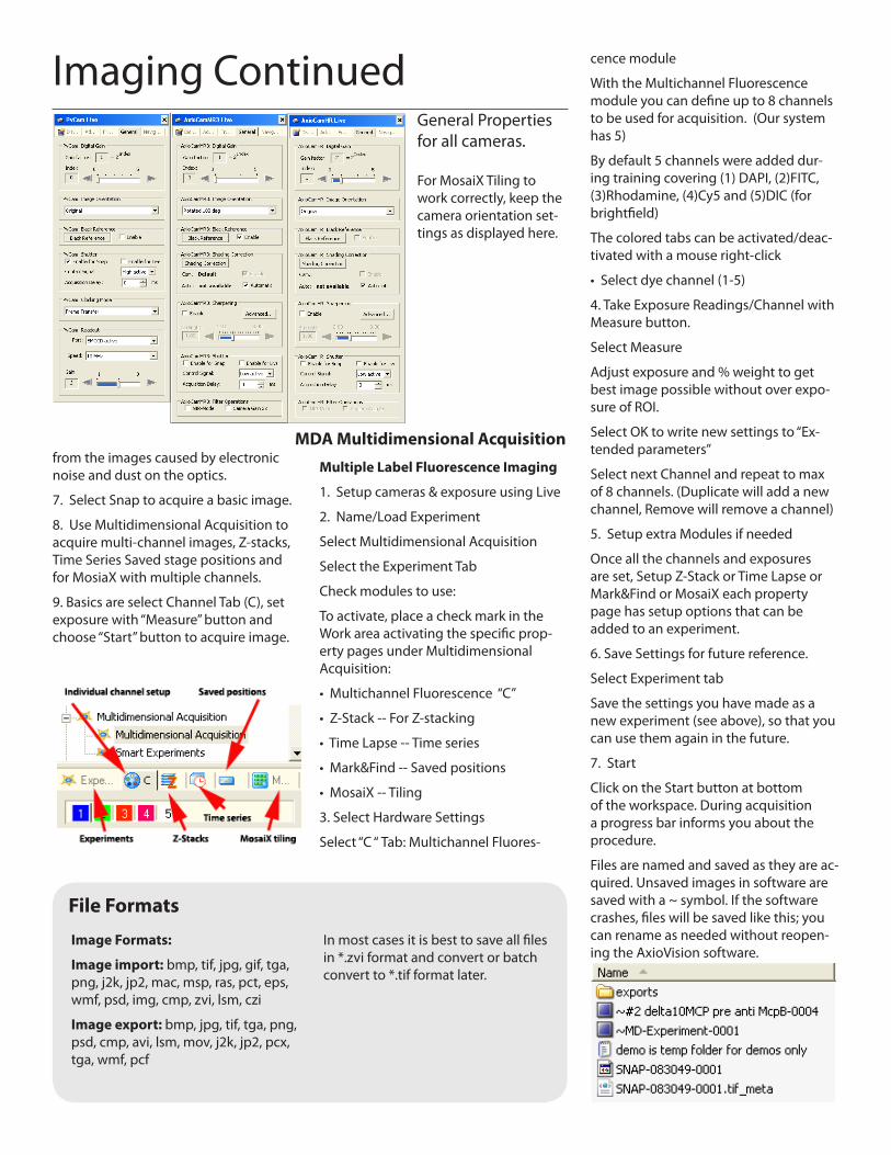
General Properties for all cameras.

For MosaiX Tiling to work correctly, keep the camera orientation set-tings as displayed here.

cence module

With the Multichannel Fluorescence module you can define up to 8 channels to be used for acquisition. (Our system has 5)

By default 5 channels were added dur-ing training covering (1) DAPI, (2)FITC, (3)Rhodamine, (4)Cy5 and (5)DIC (for brightfield)

The colored tabs can be activated/deac-tivated with a mouse right-click

• Select dye channel (1-5)

4. Take Exposure Readings/Channel with Measure button.

Select Measure

Adjust exposure and % weight to get best image possible without over expo-sure of ROI.

Select OK to write new settings to “Ex-tended parameters”

Select next Channel and repeat to max of 8 channels. (Duplicate will add a new channel, Remove will remove a channel)

5. Setup extra Modules if needed

Once all the channels and exposures are set, Setup Z-Stack or Time Lapse or Mark&Find or MosaiX each property page has setup options that can be added to an experiment.

6. Save Settings for future reference.

Select Experiment tab

Save the settings you have made as a new experiment (see above), so that you can use them again in the future.

7. Start

Click on the Start button at bottom of the workspace. During acquisition a progress bar informs you about the procedure.

Files are named and saved as they are ac-quired. Unsaved images in software are saved with a ~ symbol. If the software crashes, files will be saved like this; you can rename as needed without reopen-ing the AxioVision software.

Image Formats:

Image import: bmp, tif, jpg, gif, tga, png, j2k, jp2, mac, msp, ras, pct, eps, wmf, psd, img, cmp, zvi, lsm, czi

Image export: bmp, jpg, tif, tga, png, psd, cmp, avi, lsm, mov, j2k, jp2, pcx, tga, wmf, pcf

In most cases it is best to save all files in *.zvi format and convert or batch convert to *.tif format later.

File Formats

MDA Multidimensional Acquisition

MosaiX TilingSetup Camera

1. Select camera PvCam, AxioCam MR, Axiocam HR or Apotome Mode from Acquisition > Camera >

2. Use correct camera dialogue box to align optics to camera chosen. Button are on taskbar: Roper, Axio-MONO & Axio-COLOR.

3. Select Live from Tooolbar this will open up the “Live” Preview window. Nor-mally the Live Properties for the camera selected will pop-up too.

4. Check Image Orientation

• Select Live > Live Properties > General Tab

5. Set Exposure/Channel

• Select Measure -Measure will auto expose using settings in “extended parameters” area in Multidimensional Acquisition.

Adjust “Exposure” and “% weight” to get best image possible

Select OK to write new settings to “Ex-tended parameters”

Select next Channel and repeat to max of 8 channels. (Duplicate will add a new channel, Remove will remove a channel)

Ensure to “Flat Field” cameras to remove all artifacts present in the optic train. For the Roper camera there is a script to apply shading correction to images. This script needs to be edited individually and saved to be accessed via “extended parameters” “user interaction” submenu to get shading correction applied while running MosaiX.

The AxioCams can all have shading cor-rection applied easily under the General Tab.

Setup MosaiX

MosaiX can be run independent of Mul-tidimensional acquisition or from within it, either way the setup is the same.

1. Set Acquisition Region

MosaiX mode choices: Circular Setting

In MosaiX “Circular” mode, Columns and Rows are centered around the live im-age position at the time of setup or on Mark & Find position lists. Overlap (%) can be a low as 2% to as high as 25% or more depending on sample quality and contrast.

After choosing Rows, Columns & Over-lap(%) you can acquire image

2. Set Acquisition Region continued.

MosaiX choices: Rectangular Setting

• Rectangular allows for large regions to be acquired with focus plain adjust-ments, keeping the sample in focus from one end of the sample to the other.

• Select Live and ensure the light path is set to camera and the scalings are correct

• Select Rectangular

• Select -Setup Acquisition Setup win-

dow appears

• Select the Red X to clear previous Col-umns and Rows

Select the Four Arrows to “Mark” starting point

Move Joystick/Stage X-Y while viewing live image “Mark” ending point. The soft-ware will then calculate number of Tiles based on Overlap(%) selected.

3. Set Focus Correction

Choose a minimum of three “infocus” tiles to create an image plain.

Check focus correction box and select OK.

4. Setup Extra Modes (optional)

Any other parameters like Zstack and Time series can be set now if needed,

Example of Flat Fielding using the BS script for the Roper camera.

under Multidimensional Acquisition.

5. Start MosaiX

Click on the Start button at bottom of the workspace. During acquisition a progress bar informs you about the procedure.

Files are named and saved as they are acquired. Unsave images in software are saved with a ~ symbol.

Note: Tools > Options > (Display & Acquisition --multiple choices) can help tweak performance of the software while acquiring MosaiX tile. See Large Area Tiling.

Stitch Files Together

1. Under MosaiX in Workspace select Stitching

In most cases the default settings for the software will stitch most images

together.

Key parameters are Search Depth and Sobel Size

2. Click on the Start button at bottom of the workspace. During acquisition a progress bar informs you about the procedure.

If images do not stitch well, change the display to Tile View

Then Right click and select edit mode you can then adjust each tile individu-ally.

In many cases subtle tweaks in edit mode and then another stitch run will correct the alignment of the sample.

Reverse a stitch by:

Image = Image to be reset select and choose image.

Stitching Mode = Original positions instead of Stitching positions.

Convert Tiled image

Convert Tiled image to Single file using Convert Tile Images.

Default is the whole image.

Use this to select a region of interest.

Quick Notes

Fluorescent Tiling:

Setup Camera . . . . . . . . . . 1 . . . . . . . . . . . . . . Select Camera2 . . . . . . . . Check Image Orientation3 . . . . . . . . . . . . . . . . Flat Field4 . . . . . . . . . . Set Exposure/Channel

Setup MosaiX . . . . . . . . . . . 1 . . . . . . . . Set Acquisition Region2 . . . . . . . . . Set Focus Correction3 . . . . . . . . . . . Set Extra Modes 3 . . . . . . . . . . . . . Start MosaiX

Stitch Files Together . . . . . . . 1 . . . . . . . . . . Adjust Parameters2 . . . . . . . . . . . . . Select Start

Convert Files . . . . . . . . . . . 1 . . . . . . . . Set Region of Interest2 . . . . . . . . . Set Focus Correction3 . . . . . . . . . . . Set Extra Modes

Save Files . . . . . . . . . . . . . 1 . . . . . . . . Save to local machine2 . . . . . . . . . . Export Files as tiffs3 . . . . . . Save to Files Server (Zeus)

Large Area Tiling:

Setup Camera . . . . . . . . . .

Setup MosaiX . . . . . . . . . . .

Tweak Options Settings . . . . . . 1 . . . . . . . . Turn Off Live Window2 . . . . . . Acquisition Convert to 8bit

3 . . . . . Acquisition Prevent overview4 . . . Display No Fit Image to Window5 . . . . . . . . . . Display No Update

Max File Size . . . . . . . . . . . The maximum file size is 21,000 pixels. The software will crash at acquisitions larger than that.

The Default for the software is 4,000 pix-els but is set by ITG to 10,000 pixels. The image will be converted this maximum size using the MosaiX Convert.

Dropping the camera resolution to 8bit helps to acquire larger areas with higher magnification objectives.

Saving files

Data is saved by selecting the ‘Save As’ button at the top left corner of the AxioVision interface, or by selecting File > Save or File > Save As. Zeiss organizes files two ways: either as a single “Experiment-name file” with a “*.zvi” extension or as an experiment-name folder with grouped “Experiment-name *.zvi files” inside.

Files created with MosaiX and Time Series can get quite large so default saves and acquisitions are set to save to the local machine.

1. Save to Local Machine. --Default

You may save files to Workspace (E:\Workspace\”username”). A folder was created there at login for each user.

2. Before leaving, save to Network Share -- “username” on ‘ITG File Server (zeus.itg.uiuc.edu)’(Z:)

Most users opt to save the data to their network share on our central server (named Zeus). The server share is represented as the ‘Z:\’ drive in the windows environment. ITG is equipped with gigabit ethernet, and saving to the Z:\ drive is relatively fast. Also, this permits easy access to the data from any computer in the world using secure file transfer protocol (sftp). Instructions on accessing your network share remotely are available at http://www.itg.uiuc.edu/help/datahandling/userhelp.htm.

Saving as TIFFs (.tif )

Single images, z-scans, multi-channel images will be saved as a series of TIFF images that can be viewed in other programs (Adobe Photoshop, ImageJ, Analyze, Image Pro Plus etc…). The position in the dataset to which an image belongs is encoded into the name, thus there will be a separate TIFF image for each channel of each z-position of each time point of a dataset (assuming xyzt mode is used).

You may save Overlays, like micron bars, by selecting Burn-in annotations during Save As or Export. A text file which contains the instrument parameter settings for every image in an experiment is saved along with the individual TIFF files making up the dataset in the experiment directory.

Large files can be Batch converted without opening them up using the File > Export command

Before exporting check the Save In: location is set to either your folder in E: work-space or to Zeus

Quick Notes

Present Spatial Calibration:

Roper Cascade 512B Base Port 2.5x Bin 1 . . . . . . . . . . 5.94 mm/pixel10x Bin 1 . . . . . . . . . . 1.56 mm/pixel20x Bin 1 . . . . . . . . . . 0.78 mm/pixel40x Bin 1 . . . . . . . . . . 0.40 mm/pixel63x Bin 1 . . . . . . . . . . 0.25 mm/pixel100x Bin 1 . . . . . . . . . . .0.16 mm/pixel

Zeiss AxioCam MRm Left Port 2.5x Bin 1 . . . . . . . . . . 2.39 mm/pixel10x Bin 1 . . . . . . . . . . 0.63 mm/pixel20x Bin 1 . . . . . . . . . . 0.31 mm/pixel40x Bin 1 . . . . . . . . . . 0.16 mm/pixel63x Bin 1 . . . . . . . . . . 0.10 mm/pixel100x Bin 1 . . . . . . . . . . 0.06 mm/pixel

Zeiss AxioCam HRC Front Port 2.5x Bin 1 . . . . . . . . . . 3.91 mm/pixel10x Bin 1 . . . . . . . . . . 1.02 mm/pixel20x Bin 1 . . . . . . . . . . 0.51 mm/pixel40x Bin 1 . . . . . . . . . . 0.26 mm/pixel63x Bin 1 . . . . . . . . . . 0.16 mm/pixel100x Bin 1 . . . . . . . . . . 0.10 mm/pixel

Default file format for AxioVision is *.ZVI

Files can also be saved as *.tif

Other options are:

Image import: bmp, tif, jpg, gif, tga, png, j2k, jp2, mac, msp, ras, pct, eps, wmf, psd, img, cmp, zvi, lsm, czi

Image export: bmp, jpg, tif, tga, png, psd, cmp, avi, lsm, mov, j2k, jp2, pcx, tga, wmf, pcf

ReferencesCalibration Standards

Calibration Grid Slide from Micro Brightfield:

http://www.mbfbioscience.com

Fluorescent Reference Slides from Micros-copy Education:

http://www.microscopyeducation.com

Zeiss

http://www.zeiss.de/us/micro/home.nsf

--AxioCam HRC color CCD• Complete color information of every image detail

• 1388 x 1040 standard size, 4164x3124 Co Site Sampling

• 6.45 µm x 6.45 µm Pixel Size

• 3x14 Bit color depth and 14 Bit grey value cover-age

• Large 2/3“ CCD sensor

• Dynamic range of 2200:1

• Spectral Sensitivity approx. 400 - 700 nm

--AxioCam MRm Monochrome CCD

• 1388 x 1040 CCD basic resolution

• 6.45 μm x 6.45 μm Pixel size 12 bit

• Dynamic range of 2200:1

• Spectral Sensitivity approx. 350 nm-1000 nm

Photometrics

http://www.photomet.com/

Cascade II 512B Black & White EMCCD• Back Illuminated >90% Quatum efficiency

• 512x512 CCD array

• 16µmx16µm Pixel Size

• Frame transfer CCD

• Spectral Sensitivity approx. 350 - 1000 nm

Commercial anti-fade mounting media

• ProLong Gold Antifade Mountant:

http://www.invitrogen.co.jp/products/pdf/mp36930.pdf

• Vectashield Antifade Mounting Medium:

http://www.vectorlabs.com/VECTASHIELD/ VECTASHIELD.html

• VECTASHIELD HardSet Mounting Medium:

http://www.vectorlabs.com/products.details.asp?prodID=1483

Fluorescence Microscopy Books/Papers

Allan, V., Ed., Protein Localization by Fluo-rescence Microscopy: A Practical Approach, Oxford University Press (1999).

Andreeff, M. and Pinkel, D., Eds., Introduction to Fluorescence In Situ Hybridization: Prin-ciples and Clinical Applications, John Wiley and Sons (1999).

Conn, P.M., Ed., Confocal Microscopy (Meth-ods in Enzymology, Volume 307), Academic Press (1999).

Goldman, R.D. and Spector, D.L., Eds., Live Cell Imaging: A Laboratory Manual, Cold Spring Harbor Laboratory Press (2004).

Herman, B., Fluorescence Microscopy, Second Edition, BIOS Scientific Publishers (1998).

Hibbs, A.R., Confocal Microscopy for Biolo-gists, Springer (2004).

Matsumoto, B., Ed., Cell Biological Applica-tions of Confocal Microscopy, Second Edition (Methods in Cell Biology, Volume 70), Aca-demic Press (2003).

Michalet, X., Kapanidis, A.N., Laurence, T., Pinaud, F., Doose, S., Pflughoefft, M. and Weiss S., “The power and prospects of fluorescence microscopies and spectrosco-pies,” Annu Rev Biophys Biomolec Struct 32, 161–182 (2003).

Murphy, D.B., Fundamentals of Light Micros-copy and Electronic Imaging, John Wiley and Sons (2001). Molecular Probes

Ntziachristos, V., “Fluorescence molecular im-aging,” Annu Rev Biomed Eng 8, 1–32 (2006).

Pawley, J.B., Ed., Handbook of Biological Confocal Microscopy, Third Edition, Springer (2006).

Periasamy, A., Ed., Methods in Cellular Imag-ing, Oxford University Press (2001).

Rizzuto, R., and Fasolato, C., Eds., Imaging Living Cells, Springer-Verlag (1999).

Spector, D.L. and Goldman, R.D., Basic Methods in Microscopy, Cold Spring Harbor Laboratory Press (2005).

Stephens, D., Ed., Cell Imaging (Method Ex-press Series), Scion Publishing (2005).

Yuste, R. and Konnerth, A., Eds., Imaging in Neuroscience and Development: A Labora-tory Manual, Cold Spring Harbor Laboratory Press (2004).

B&W Camera Quantum Efficiency

Imaging Technology Group

Beckman Institute for Advanced Science and Technology

University of Illinois at Urbana-Champaign

405 North Mathews, Urbana IL 61801 USA

Phone: 217.244.0170 FAX: 217.244.6219

Chroma Filter Sets for Axiovert 200M

Starndard set in Axiovert 200M

Default Reflector Turret set to:(1) 350EX/460EM DAPI Chroma Set 31000V2(2) 470EX/515EM FITC Chroma Set 41025(3) 560EX/620EM Rhodamine Chroma Set 41039(4) C5 640EX/680EM Cy5 Chroma Set 31023(5) Transmitted DIC cube

Alternative set for Axiovert 200M

Second Reflector Turret set to:(1) Custum 350EX/565EM Chroma Set 31000V2 with 565 Emitter(2) Qdot 605nm Chroma Set 32007(3) Qdot 655nm Chroma Set 32012(4) Reflected Darkfield cube(5) Reflected Brightfield cube

Filter Cube Box for Axiovert 200M

(1) Custum Zeiss Apotome Calibration Cube(2) 425EX/540EM Lucifer Yellow Chroma Set 31010(3) 780EX/800EM Li-Cor Chroma Set 41037(4) Custum UV blocking 400DCLP & GG400LP EM(5)(6)

Turret Position 1

Turret Position 2

Turret Position 3

Turret Position 4