Embed Size (px)
Citation preview

This content has been downloaded from IOPscience. Please scroll down to see the full text.
Download details:
IP Address: 128.122.253.228
This content was downloaded on 10/10/2014 at 13:58
Please note that terms and conditions apply.
The flavor of the composite pseudo-goldstone Higgs
View the table of contents for this issue, or go to the journal homepage for more
JHEP09(2008)008
(http://iopscience.iop.org/1126-6708/2008/09/008)
Home Search Collections Journals About Contact us My IOPscience

JHEP09(2008)008
Published by Institute of Physics Publishing for SISSA
Received: June 27, 2008
Accepted: August 16, 2008
Published: September 1, 2008
The flavor of the composite pseudo-goldstone Higgs
Csaba Csaki,ab Adam Falkowskicd and Andreas Weilerab
aInstitute for High Energy Phenomenology,
Newman Laboratory of Elementary Particle Physics,
Cornell University, Ithaca, NY 14853, U.S.A.bKavli Institute for Theoretical Physics,
University of California, Santa Barbara, CA 93106, U.S.A.cCERN Theory Division, CH-1211 Geneva 23, SwitzerlanddInstitute of Theoretical Physics, Warsaw University,
Hoza 69, 00-681 Warsaw, Poland
E-mail: [email protected], [email protected],
Abstract: We study the flavor structure of 5D warped models that provide a dual de-
scription of a composite pseudo-Goldstone Higgs. We first carefully re-examine the flavor
constraints on the mass scale of new physics in the standard Randall-Sundrum-type sce-
narios, and find that the KK gluon mass should generically be heavier than about 21 TeV.
We then compare the flavor structure of the composite Higgs models to those in the RS
model. We find new contributions to flavor violation, which while still are suppressed by
the RS-GIM mechanism, will enhance the amplitudes of flavor violations. In particular,
there is a kinetic mixing term among the SM fields which (although parametrically not
enhanced) will make the flavor bounds even more stringent than in RS. This together
with the fact that in the pseudo-Goldstone scenario Yukawa couplings are set by a gauge
coupling implies the KK gluon mass to be at least about 33 TeV. For both the RS and
the composite Higgs models the flavor bounds could be stronger or weaker depending on
the assumption on the value of the gluon boundary kinetic term. These strong bounds
seem to imply that the fully anarchic approach to flavor in warped extra dimensions is
implausible, and there have to be at least some partial flavor symmetries appearing that
eliminate part of the sources for flavor violation. We also present complete expressions for
the radiatively generated Higgs potential of various 5D implementations of the composite
Higgs model, and comment on the 1 − 5 percent level tuning needed in the top sector to
achieve a phenomenologically acceptable vacuum state.
Keywords: Beyond Standard Model, Quark Masses and SM Parameters, Field Theories
in Higher Dimensions, Kaon Physics.
c© SISSA 2008

JHEP09(2008)008
Contents
1. Introduction 1
2. Flavor in RS 3
3. 5D models for pseudo-goldstone Higgs 10
3.1 Spinorial 12
3.2 Fundamental + Adjoint 13
3.3 Four-fundamental 14
4. Higgs potential 15
4.1 Constraints from electroweak precision tests 23
5. Flavor in GHU 25
5.1 Fermion masses and mixing 25
5.2 Flavor constraints 28
5.3 Numerical scan 31
5.4 Fermions in the spinorial 32
5.5 Fermions in four fundamentals 32
6. Conclusion 33
A. KK gluon sums 35
B. SO(5) generators 36
B.1 Spinorial 36
B.2 Fundamental 37
B.3 Adjoint 37
1. Introduction
Warped extra dimensions models were introduced by Randall and Sundrum (RS) [1] as
an attempt to solve the hierarchy problem by making use of the warp factor to lower
the natural scale of particle masses. In the original model, all SM fields were localized
on the TeV brane. By the AdS/CFT duality, this corresponds to a situation where a
strongly coupled 4D conformal field theory spontaneously breaks conformality at the TeV
scale, creates a mass gap (confines), and produces the SM fields as approximately massless
composites. One consequence of this scenario is the CFT cannot be flavor invariant, since it
is supposed to produce the Yukawa couplings among the SM fields. In such a case, however,
– 1 –

JHEP09(2008)008
the CFT is also expected to generate higher-dimensional flavor violating operators with
only a TeV suppression, which would be disastrous from the phenomenological point of
view. Phrased in the 5D language this question is why generic TeV localized four-fermion
operators are suppressed by some high scale, rather than the local cut-off scale which is a
few TeV.
This severe flavor problem can be avoided by instead considering setups with the SM
gauge fields and fermions in the bulk, and only the Higgs sharply localized on the TeV
brane [2 – 4]. In this case the SM fermions can be thought of as mixtures of elementary and
composite fermions. The amount of mixing is determined by the profile of the 5D wave
function of the fermions: the more peaked they are close to the Planck brane, the more
elementary are these fields. This sheds some light on the flavor puzzle as well: Although
the Yukawa couplings generated by the CFT are indeed all O(1) and non-diagonal, the
fermion masses and the CKM angles depend also on the amount of mixing of the elementary
fermions with the CFT that is assumed to be small for the first two generations [3 – 5]. Most
importantly, this implies that flavor violation in the SM is also suppressed by the same
mixing factors - the fact that goes under the name of the RS-GIM mechanism [4, 6, 7],
see also [8, 9]. RS-GIM is successful in suppressing most of the dangerous flavor-changing
neutral currents (FCNC) [6], although it is not enough to sufficiently suppress new physics
contributions to CP violation in the kaon sector [11, 10].
Although the RS set-up explains the origin of the large MPL/TeV hierarchy, there
still remains the little hierarchy problem, which amounts to the question why the Higgs
boson is much lighter than a few TeV. In RS, the Higgs is realized as a scalar field localized
on the TeV brane, of which the 4D dual interpretation is that Higgs a composite state
of the CFT. In that case, its mass would naturally be at the CFT scale of a few TeV,
which would effectively produce a Higgsless model of the sort considered in [12]. One way
to obtain a light composite Higgs is by making it a pseudo-Goldstone boson (pGB) of a
global symmetry [13], similarly as in little Higgs models [14]. The 5D holographic version
of this scenario are the models of gauge-Higgs unification (GHU) [15], where the Higgs
boson is identified with the fifth component of a bulk gauge field (A5) [16]. The Higgs
potential is radiatively generated (with the largest contributions due to the top and gauge
multiplets) and fully calculable. The most promising scenario of this kind is based on the
SO(5) gauge group in the bulk, broken spontaneously to SO(4) on the TeV brane [17], and
with an implementation of a discrete parity symmetry to control corrections to the Zbb
vertex [18]. This is the minimal scenario that passes the stringent electroweak precision
tests.
Thus, GHU provides us with the Higgs sector that allows one to address both the
large and the little hierarchy problem. It is a natural question to ask how this dynamical
realization of the Higgs boson affects the flavor structure and the RS-GIM mechanism.
This is the subject of this paper.
Perhaps not surprisingly, the flavor structure of GHU turns out to be quite similar to
that in RS. However, there are some important differences, that affect the flavor bounds.
The gauge symmetry must be larger than in RS (to include broken generators that give rise
to the pseudo-Goldstone Higgs degrees of freedom), which results in a different embedding
– 2 –

JHEP09(2008)008
of the SM fermion into the bulk representation. In particular, one SM fermion must be
embedded in several bulk multiplets. This induces a new effect not present in RS, namely
that, in the original flavor basis, the various fermionic generations are mixed via kinetic
terms. This kinetic mixing is a new source of flavor violation in GHU which is always non-
zero (as long as the CKM mixing is reproduced). Even though the kinetic mixing respects
the RS-GIM mechanism, it results in an enhancement of the flavor violating operators. As
a consequence, the bounds on the scale of the extra dimensions from flavor physics turn
out to be more stringent compared to the RS case.
This paper is organized as follows: in section 2 we review the flavor structure and
the RS-GIM mechanism of ordinary RS models with gauge and fermions in the bulk and
the Higgs on the TeV brane. We reevaluate the bounds on the mass of the KK gluon
and find it has to be ≥ 22 TeV for anarchic Yukawa couplings. In section 3 we review
the basics of the GHU models and then define three different realizations based on the
SO(5) gauge symmetry in the bulk. Before investigating the flavor structure, we study
the constraints on the parameter space of these models imposed by the requirement of
correct electroweak symmetry breaking. In section 4 we calculate the Higgs potential for
the three SO(5) models. We re-emphasize that one of the parameters of the top sector has
to be tuned at the 1-5 percent level to end up with a realistic scenario, which is a new
guise of the little hierarchy problem specified to GHU models. These relations among the
parameters of the model are then used as an input in our studies of the flavor bounds.
Section 5 contains our main results. There we present the flavor structure of the SO(5)
models under investigation, and pinpoint new sources of flavor violation. We estimate the
magnitude of flavor and CP violation induced by the KK gluon exchange and illustrate our
analytical estimates by numerical scans over the parameter space allowed by electroweak
symmetry breaking. We conclude with some remarks on future directions of GHU in light
of our findings.
2. Flavor in RS
The original motivation for considering warped extra dimension was the solution to the
hierarchy problem of the Higgs sector. It was quickly realized that the set-up also has
the potential to explain simultaneously the SM flavor structure. Starting with completely
anarchic Yukawa coupling of the Higgs and the 5D fermions, the large SM fermion mass
hierarchies can be explained by different localization the SM fermions in the extra dimen-
sion [3, 4, 19], implementing the split fermion scenario of [20]. Small mixing angles of the
CKM matrix are a natural consequence of this scenario [5]. Moreover, this way of gener-
ating flavor mass hierarchies automatically implies a certain amount of suppression of the
dangerous flavor changing, which is referred to as the RS-GIM mechanism. In this section
we will review the flavor bounds on the generic RS models with anarchic flavor structure.
This will provide us with a reference point for our study of the flavor bounds in the GHU
models.
We specify the background metric to be AdS5 space. We parametrize the space-time
– 3 –

JHEP09(2008)008
by the conformal coordinates
ds2 =
(
R
z
)2
(dxµdxνηµν − dz2) , (2.1)
where the AdS curvature is R, and the coordinate z of the extra dimension runs between
R < z < R′, z = R corresponding to the UV (Planck) brane and z = R′ to the IR (TeV)
brane. R′/R ∼ 1016 sets the large hierarchy between the Planck and the TeV scale.
We consider here the standard RS scenario with custodial symmetry [21] (this is always
what we mean when we refer to RS in the following). The bulk gauge group SU(3)C ×SU(2)L × SU(2)R ×U(1)X and the Higgs field transforming as (1, 2, 2)0 is localized on the
TeV brane. The fermionic content includes three copies of Ψiq, i = 1 . . . 3, transforming as
(2, 1)1/6 , and 3 copies each of Ψiu,d in (1, 2)1/6. Each of these fields are 5D bulk Dirac spinors
and have a bulk mass term which is customarily parametrized by using the c-parameters,
(
R
z
)4[
ciqz
ΨiqΨ
iq +
ciuz
ΨiuΨi
u +cidz
ΨidΨ
id
]
. (2.2)
From now on we drop the generation index i; all fermions should always be understood
as three-vectors in the generation space. The boundary conditions on the UV and the IR
brane are chosen as
Ψq =(
q[+,+])
Ψu =
(
uc[−,−]
dc[+,−]
)
Ψd =
(
uc[+,−]
dc[−,−]
)
(2.3)
where [±] denotes the right(left)-chirality of a bulk fermion vanishing on the brane. The SM
quark doublets are realized as zero-modes q, while the singlets up and down-type quarks
are zero modes of uc and dc, respectively. We write it as
q(x, z) → χq(z)qL(x) uc(x, z) → ψu(z)uR(x) dc(x, z) → ψd(z)dR(x) (2.4)
where χq(z) and ψu,d(z) are the zero mode profiles that are obtained by solving the equa-
tions of motion. A normalized left-handed zero-mode profile is given by
χc(z) = R′−1/2( z
R
)2 ( z
R′
)−cf(c), ψc(z) = R′−1/2
( z
R
)2 ( z
R′
)cf(−c) . (2.5)
We have introduced the standard RS flavor function f(c), which is given by
f(c) =
√1 − 2c
[
1 − (R′
R )2c−1]
1
2
. (2.6)
We also introduce 3×3 diagonal matrices fc that are constructed from f(ci) of three genera-
tions, for example fq = diag(f(cq1), f(cq2
), f(cq3)). For the choice of the c-parameters that
reproduce the SM mass hierarchies the matrices fq,−u,−d are exponentially hierarchical.
The masses of the zero modes come from the IR brane-localized Yukawa interactions.
After the Higgs field acquires a vev, the Yukawa terms lead to IR localized mass terms for
the bulk fermions,
Ly = − v√2(R4/R′3)
(
ΨqYuΨu + ΨqYdΨd
)
+ h.c. (2.7)
– 4 –

JHEP09(2008)008
value at 3TeV
mu 0.00075 . . . 0.0015
mc 0.56 ± 0.04
mt 136.2 ± 3.1
md 0.002 . . . 0.004
ms 0.047 ± 0.012
mb 2.4 ± 0.04
Table 1: MS quark masses in GeV at 3 TeV. We have taken the ranges and low-energy values
from PDGLive [22] and used LO renormalization equations with the appropriate number of flavors
for the rescaling. At 30TeV, the masses mi are about 11% smaller.
The brane Yukawa couplings Yu,d are assumed to be anarchic — random matrices with
elements O(1), no hierarchy and O(1) determinant.
Inserting the zero mode profiles into the mass terms in eq. (2.7) we obtain the SM
mass matrices
mSMu =
v√2fqYuf−u,
mSMd =
v√2fqYdf−d, (2.8)
From this point on the usual SM prescription applies. We diagonalize the up and down
mass matrices by mSMu,d = UL u,dmu,dU
†R u,d, where U ’s are unitary and mu,d are diagonal,
and we rotate the zero modes to the mass eigenstate basis, for example dL(x) → UL ddL(x).
The left rotations yield the CKM matrix, VCKM = U †L uUL d.
Even though the Yukawa matrices are anarchical, the hierarchical matrices fc introduce
the hierarchy into the mass matrix elements.
This will result in the hierarchy of the eigenvalues:1
(mu,d)ii ∼v√2Y∗fqi
f−ui,di(2.9)
where Y∗ is the typical amplitude of the entries in the Yukawa matrices. One can also show
that the diagonalization matrices themselves are hierarchical [5]:
|UL ij | ∼fqi
fqj
, |UR ij| ∼f−u,di
f−u,dj
, i ≤ j. (2.10)
We also get that |VCKM|ij ∼ fqi/fqj
, thus the hierarchy in the CKM matrix elements is
purely set by the cq parameters. From experiment we know that the hierarchy of the CKM
matrix is of the form
VCKM ∼
1 − λ2
2 λ λ3
λ 1 − λ2
2 λ2
λ3 λ2 1
(2.11)
1Here and in the following, the quark masses are understood as running masses at the scale at which
the extra dimension is integrated out. We choose the scale of the extra dimension to be 3TeV. In table 1
we collect all input values at this scale.
– 5 –

JHEP09(2008)008
where λ ∼ sin θC ∼ 0.2. This fixes the hierarchy among the fqi’s to be [5]
fq2/fq3
∼ λ2, fq1/fq3
∼ λ3. (2.12)
The values of f−u,−d are then fixed by requiring that the correct fermion mass hierarchy is
reproduced, implying the following relations (assuming f−u3∼ O(1)):
f−d3∼ mb
mt, f−u2
∼ mc
mt
1
λ2, f−d2
∼ ms
mt
1
λ2, f−u1
∼ mu
mt
1
λ3, f−d1
∼ md
mt
1
λ3. (2.13)
Thus, the RS set-up leads to a neat explanation of the SM flavor structure. However, one
potentially worrisome feature of higher-dimensional models is the presence of the new KK
states, whose masses are in the TeV range (as long as the hierarchy problem is addressed).
These new states generically have flavor non-universal couplings and will contribute to
flavor-changing neutral currents.
The largest contribution to flavor changing neutral currents is generated via the ex-
change of heavy gauge bosons, in particular the strongest constraint arises from the ex-
change of the KK gluons. In order to calculate the effective four-Fermi operators we first
need to determine the couplings gx of the zero-modes to the KK gluons,
gijL,uu
iLγµG
µ(1)ujL + gij
L,ddiLγµG
µ(1)djL + (L→ R) (2.14)
Below we discuss the contribution of the lightest KK gluon but, as we show in appendix A,
it is possible to sum up the contribution of the entire gluon KK tower. The profile of the
first KK gluon can be approximated by G(1)(z) ≃√
2J1(x1)
√RR′
zJ1(x1z/R′) with x1 being
the first zero of the Bessel function, J0(x1) = 0. Using this and the zero mode profiles
we can determine the couplings in eq. (2.14). In the original flavor basis the couplings are
diagonal and well approximated by
gx ≈ gs∗
(
− 1
logR′/R+ f2
x γ(cx)
)
. (2.15)
where gs∗ is the bulk SU(3) gauge couplings, and γ(c) =√
2x1
J1(x1)
∫ 10 x
1−2cJ1(x1x)dx ≈√
2x1
J1(x1)0.7
6−4c .2 The couplings would be flavor universal if fx ∼ 13×3. However, this not
the case in the RS scenario where the fx are non-degenerate. This is the main source of
flavor violation in RS. Going to the mass eigenstate basis, we have to rotate the couplings
appropriately,
gL,u,d → U †L u,dgqUL u,d gR,u,d → U †
R u,dg−u,−dUR u,d (2.16)
The rotation introduces non diagonal couplings which lead to tree level contributions to
∆F = 2 processes. Nevertheless, the rotation matrices are hierarchical, with the hierarchy
set by the same fx that controls the SM fermion hierarchies. The off-diagonal KK gluon
couplings are of order
(gL,q)ij ∼ gs∗fqifqj
(gR,u)ij ∼ gs∗f−uif−uj
(gR,d)ij ∼ gs∗f−dif−dj
(2.17)
2The function γ(c) is a correction to the approximation used in [6] which can be sizable, e.g. γ(−0.4) ≈
0.52, γ(0.5) ≈ 1.16, γ(0.7) ≈ 1.52. In numerical calculations we always use the full overlap integral.
– 6 –

JHEP09(2008)008
The off-diagonal couplings of the quark doublets are suppressed by the ratios of the CKM
matrix elements (recall that fq1∼ λ3, fq2
∼ λ2). Similarly, the off-diagonal couplings of the
singlet quarks are suppressed by hierarchically small entries. This suppression is called the
RS-GIM mechanism. It is enough to suppress most of the dangerous ∆F = 2 operators,
though not all, as we will see in a moment.
Integrating out the KK gluon and applying appropriate Fierz identities we obtain the
effective Hamiltonian:
H =1
M2G
[
1
6gijL g
klL (qiα
L γµqjLα) (qkβ
L γµqlLβ)
−gijRg
klL
(
(qiαR q
kLα) (qlβ
L qjRβ) − 1
3(qiα
R qlLβ) (qkβ
L qjRα)
)]
= C1(MG)(qiαL γµq
jLα) (qkβ
L γµqlLβ)
+C4(MG)(qiαR q
kLα) (qlβ
L qjRβ) + C5(MG)(qiα
R qlLβ) (qkβ
L qjRα)
where α, β are color indices. The Wilson coefficients of these operators will directly corre-
spond to the C1,4,5 bounded by the model independent constraints from ∆F = 2 processes
by the UTFit collaboration3 in [11], see table 2.
Note, that the most strongly constrained quantity is the imaginary part of C4K for the
kaon system. Contributions to ǫK coming from C4K are enhanced compared to the ones to
C1K with SM like chirality by
∼ 3
4
(
mK
ms(µL) +md(µL)
)2
η−51 (2.18)
where the first factor ≈ 18 is the chiral enhancement of the hadronic matrix element and
η−51 ≈ 8 is the relative RGE running [23].
We are ready to estimate the flavor bounds of the RS model. Using the expressions for
the orders of magnitudes for the rotation matrices U we approximately find for the Wilson
coefficient at the TeV scale
CRS4K ∼ g2
s∗M2
G
fq1fq2f−d1
f−d2∼ 1
M2G
g2s∗Y 2∗
2mdms
v2. (2.19)
Above, md,ms are the down, strange masses at the TeV scale, see table 1. At tree level
and in absence of boundary kinetic terms, the bulk coupling gs∗ is connected the strong
coupling at the KK scale by gs∗ = gs(MG) log1/2(R′/R) ∼ 6. If arbitrary large Y∗ was
allowed the bounds from C4K could be eliminated completely. However, if Y∗ is too large
one loses perturbative control over the theory. One can estimate the upper bound on Y∗using naive dimensional analysis. The proper brane localized Yukawa coupling Y5D is in our
normalization Y5D = Y∗R′. One-loop corrections to the localized Yukawa coupling would
be proportional to Y5D(Y5DE)2/(16π2), where the energy dependence is inferred from the
dimension −1 of Y5D. In order for this to be smaller than the tree-level term we need to
impose (Y5DE)2/(16π2)<∼ 1. We require that this bound is not violated until we reach the
3We are grateful to Luca Silvestrini for discussions about the proper interpretation of the UTFit bounds.
– 7 –

JHEP09(2008)008
Parameter Limit on ΛF (TeV) Suppression in RS (TeV)
ReC1K 1.0 · 103 ∼ r
√6/(|VtdVts|f2
q3) = 23 · 103
ReC4K 12 · 103 ∼ r(vY∗)/(
√2mdms) = 22 · 103
ReC5K 10 · 103 ∼ r(vY∗)
√3/(
√2mdms) = 38 · 103
ImC1K 15 · 103 ∼ r
√6/(|VtdVts|f2
q3) = 23 · 103
ImC4K 160 · 103 ∼ r(vY∗)/(
√2mdms) = 22 · 103
ImC5K 140 · 103 ∼ r(vY∗)
√3/(
√2mdms) = 38 · 103
|C1D| 1.2 · 103 ∼ r
√6/(|VubVcb|f2
q3) = 25 · 103
|C4D| 3.5 · 103 ∼ r(vY∗)/(
√2mumc) = 12 · 103
|C5D| 1.4 · 103 ∼ r(vY∗)
√3/(
√2mumc) = 21 · 103
|C1Bd
| 0.21 · 103 ∼ r√
6/(|VtbVtd|f2q3
) = 1.2 · 103
|C4Bd
| 1.7 · 103 ∼ r(vY∗)/(√
2mbmd) = 3.1 · 103
|C5Bd
| 1.3 · 103 ∼ r(vY∗)√
3/(√
2mbmd) = 5.4 · 103
|C1Bs
| 30 ∼ r√
6/(|VtbVts|f2q3
) = 270
|C4Bs
| 230 ∼ r(vY∗)/(√
2mbms) = 780
|C5Bs
| 150 ∼ r(vY∗)√
3/(√
2mbms) = 1400
Table 2: Lower bounds on the NP flavor scale ΛF for arbitrary NP flavor structure from [11] and
the effective suppression scale in RS for KK mass with MG = 3 TeV. Since the Wilson coefficients
in [11] are given at the scale ΛF , we have corrected for the renormalization group scaling from
ΛF to 3 TeV using the expressions in [23] when necessary. We have set |Y∗| ∼ 3, fq3= 0.3 and
r = MG/gs∗.
energies N KK modes, E = NKKmKK. Using mKK ∼ 2/R′ we find that Y∗<∼(2π)/NKK. For
the most conservative bound we set NKK = 2, which imposes Y∗<∼3. Thus in our estimates
we assume |Y∗|<∼3. The suppression scale of the four-fermion operator is set by the lightest
KK gluon mass MG. The RS-GIM mechanism effectively raises the suppression scale by
the factor v/√mdms ∼ 104. However, that factor turns out to be an order of magnitude
too small for a ∼ 3TeV KK gluon. One can find that in order for the suppression scale
to match 1.6 · 105 TeV we need MG ∼ (22 ± 6) TeV. Our estimate is less optimistic than
that encountered in the RS literature so far [10, 24, 25]. The quoted error comes from the
uncertainty in the md and ms masses. Including the contributions of the full KK gluon
tower may change our result by less than 10%.
In order to understand the actual flavor bound on the RS model in more detail we
have generated a sample of points with randomly chosen values of 1/R′ and brane Yukawa
– 8 –

JHEP09(2008)008
Figure 1: Scan of the effective suppression scale of ImC4K in the RS model. All the points give the
correct low-energy spectrum but most of the points with mG < 21TeV fail to satisfy the bound of
Λ > 1.6 ·105 TeV. The blue line is a linear fit of the MG dependence. We have taken cq3∈ [0.4, 0.45],
cu3∈ [−0.3,−.05], cd3
= −0.55 and |Y∗| ∈ [1, 3].
couplings of which we selected 500 where the masses, the absolute values of the CKM
elements and the Jarlskog invariant approximately matches the SM prediction. We then
calculate the exact flavor suppression scale for the C4K operator. The result is presented
in figure 1. We can say that, in accordance with our analytical estimates, as long as MG is
below 21 TeV the majority of the generated points violate the flavor bound. This turns the
”coincidence problem” of RS [6] into a fine tuning problem: unless there is some additional
flavor structure one is likely to violate the flavor bounds.
Note, that there is a model dependence that can strengthen or weaken the above
obtained bound: the matching of the bulk gauge coupling to the strong coupling can be
changed by adding localized kinetic terms for the gluon
1
g2s(q)
=logR′/R
g2s∗
+1
g2s,UV (q)
+1
g2s,IR(q)
(2.20)
A positive brane kinetic term would make the KK gluon more strongly coupled, which
would make the flavor bounds more severe. However, the UV brane coupling can be
effectively negative at the TeV scale, if one includes the 1-loop running effects [38],4
1
g2s,UV (q)
=1
g2s,UV (1/R)
− bUV3
8π2log(1/qR) (2.21)
where bUV3 is the QCD beta functions of the zero modes localized around the UV branes.
The running of the IR brane localized kinetic term is cut off at the scale ∼ 1/R′ therefore
it will not involve a large logarithm and we will neglect the IR brane localized terms, and
focus only on the UV brane localized kinetic terms. Assuming that the top is localized on
4We thank Kaustubh Agashe and Roberto Contino for pointing this out.
– 9 –
JHEP09(2008)008
the TeV brane, and all other fields on the UV brane for QCD we find bUV3 = 8. Thus, the
asymptotically free QCD running reduces the magnitude of gs∗ and thus the coefficient of
the operators induced by the KK gluon exchange, while a bare UV brane localized kinetic
term would enhance the effect. Our 21 TeV bound presented above corresponds to a choice
of boundary kinetic terms where the bare UV couplings exactly cancels the contribution
from the running. Another possibility would be to assume no UV boundary kinetic term at
the Planck scale. In that case the coupling of the KK gluon is much weaker, changes from
gs∗ ≈ 6 to gs∗ ≈ 3, and the bound is reduced by a factor of ∼ 2 from 21 TeV to 10.5 TeV.
Yet another possibility is to pick a large bare UV coupling such that the bulk is strongly
coupled, gs∗ ∼ 4π. This would enhance the flavor bound on the KK gluon mass by a factor
of ∼ 2 from 21 TeV to 42 TeV.
In the remainder of this paper we investigate how the flavor bounds are modified in
5D models where the electroweak breaking sector arises dynamically.
3. 5D models for pseudo-goldstone Higgs
In this section we introduce the 5D framework of GHU and define particular models whose
flavor structure we will later study. The basic ingredient of GHU is the presence of a zero
mode along the scalar (Az) direction of the bulk gauge field. This mode is identified with
the SM Higgs boson. The idea of GHU has a long history going back to Manton and
Hosotani [15]. More recently, GHU has been formulated in 5D warped space-time [26, 16,
17] which, among other things, allows one to obtain a heavy enough top quark. Other
important developments are related to electroweak precision observables (EWPO’s). The
S-parameter is within the experimental bounds if the KK scale of the theory is raised to
2-3 TeV [17]. The ρ-parameter can be protected by custodial symmetry, and the discrete
L↔ R symmetry protecting the Zbb vertex can be implemented [28].
The simplest GHU model with custodial symmetry is based on the SO(5) × U(1)X(plus the color group) bulk gauge group which is broken via boundary conditions to the
SM group SU(2)L ×U(1)Y on the UV brane and to SO(4)×U(1)X on the IR brane, where
SO(4) ∼SU(2)L×SU(2)R. The fact that the SO(5)/SO(4) coset generators are broken on
both branes results in four zero modes with the quantum numbers of the SM Higgs doublet.
At tree-level, these modes are massless due to 5D gauge invariance, but at one loop they
develop a potential.
We denote the dimensionful gauge coupling of SO(5) by g∗R1/2. A useful measure of
the magnitude of g∗ is the number of colors of the dual CFT by
NCFT =16π2
g2∗
(3.1)
The 5D description is perturbative as long as NCFT ≫ 1. We also allow for a UV brane
localized gauge kinetic terms for SU(2)L (for simplicity, we set the U(1)Y brane kinetic
term to zero) and parametrize it by 1/g2UV = r2 log(R′/R)/g2
∗ . The SU(2)L coupling is
then related to the 5D parameters by
g =g∗
log1/2(R′/R)√
1 + r2(3.2)
– 10 –

JHEP09(2008)008
For a small brane kinetic term, r ≪ 1, and the Planck-TeV hierarchy, log(R′/R) ∼ 37, we
need the bulk coupling g∗ ≈ 4 (corresponding to NCFT = 10) in order to reproduce the
SM weak coupling. With the brane kinetic term we have to make the bulk more strongly
coupled, in particular for r2 = 4 we go down to NCFT = 2.
The four components ha of the Higgs doublet are embedded into the gauge field A5 as
Az(z) =
√
2
R
z
R′TaCh
a(x) (3.3)
Here, the T aC ’s are the generators of the SO(5)/SO(4) coset. The normalization is chosen
such that ha’s have the canonical kinetic terms in the 4D effective theory. We fix the Higgs
vev along the h4 direction, and we denote 〈h4〉 = v.
The 5D model has two important scales that play a vital role in the dynamics. One is
R′ which sets the KK scale, and the masses of the lightest KK modes of electroweak gauge
bosons are roughly ∼ 2.4R′. Another important quantity is the global symmetry breaking
scale fπ (or the ”Higgs decay constant”) defined by
fπ =2
g∗R′ =2
g√
logR′/R√
1 + r2R′. (3.4)
Because the logarithm is large, fπ < R′ by at least a factor of ∼ 2. The W-mass is
connected to the scale fπ and the Higgs vev via
M2W =
g2f2π
4sin2(v/fπ) (3.5)
For v ≪ fπ, once recovers the SM formula M2W ≈ g2v2/4.
Fixing the gauge group still leaves several options for realizing the fermionic sector of
the theory, depending on how the SM quarks are embedded into SO(5) representations.
In this paper we consider three distinct realizations that have previously appeared in the
literature. Before we move to the detailed description of the model we point a few general
model-building rules that we need follow.
• The SM quarks are identified with the zero modes of 5D quarks. The presence of
zero modes depends on the boundary conditions. There are two possibilities: either
we choose the right-handed chirality of the 5D fermion to vanish on a boundary
(which is denoted as [+]), or the left-handed chirality vanishes (denoted as [−]).
Left-handed zero modes - appropriate for SM doublet quarks - arise whent the right-
handed chirality vanishes on both the UV and the IR brane, the choice denoted as
[++]. The [−−] boundary conditions lead to right-handed zero modes appropriate
for the SU(2)L singlet SM quarks.
• Each of the SM quarks should be embedded in a separate SO(5) multiplet. In principle,
SO(5) multiplets contain fields with the quantum numbers of both doublet and singlet
quarks. However, multiplets that yield both doublet left-handed zero modes and
singlet right-handed zero modes are problematic for the following reason. For the
first two generations, if the left-handed zero mode is localized close to the UV brane,
– 11 –

JHEP09(2008)008
then the right handed zero mode is localized at the IR brane, which leads to problems
with precision measurements. For the third generation, the reason is more subtle and
has to do with the radiative generation of the Higgs potential; we will comment on
that later. Thus, we need at least three SO(5) multiplets for each generation. As a
consequence, the field content of GHU models is necessarily larger than that of RS.
• Apart from the zero mode, the remaining fields in the multiplets should yield only
heavy KK modes. One should take care that the boundary conditions do not lead to
ultra-light KK modes. This may happen for the quarks living in the same multiplet
with UV localized zero modes, depending on the boundary conditions of the remaining
fields. The rule of thumb is that SO(5) partners of [++] fields should be assigned
[−+] boundary conditions, while the partners of [−−] fields should have [+−].
• This zeroth-order picture is modified by the mass terms on the IR brane that mix
different 5D multiplets. These mass terms are necessary to arrive at acceptable
phenomenology. First of all, since the Higgs field is a component of Az, it only
couples 5D quarks from the same bulk multiplet. In order to obtain non-zero quark
masses, at least some of the zero modes should have non-vanishing components in
more than one multiplet. The boundary mass terms play a similar role as the Yukawa
couplings in RS but, as we discuss later, there are some important differences.
• At the end of the day, the boundary conditions to SO(5) multiplets should be such
that SO(5) is broken on both the UV and the IR branes. The Wilson-line breaking is
a non-local effect that is operating only when the gauge symmetry is broken on both
endpoints of the fifth dimension. If either the UV or the IR boundary conditions are
SO(5) symmetric, the Wilson line can be rotated away, and the SM quarks do not
acquire masses.
We move to discussing three specific realizations that satisfy the above requirements.
3.1 Spinorial
The spinor representation 4 is the smallest SO(5) representation. Although models with
the third generation embedded in the spinorial representation have severe problems with
satisfying the precision constraints on the Zbb vertex, we do include it in our study. The
reason is that this model is the simplest (it has the minimal number of bulk fields), and its
flavor structure is most transparent. Furthermore, almost identical flavor structure appears
in the fully realistic models.
We consider 3 bulk SO(5) spinors for a single generation of quarks, Ψq,Ψu,Ψd (recall
that we omit the generation index; all fermionic fields should be read as three-vectors in the
generation space). Under the SU(2)L×SU(2)R subgroup it splits as 4 → (2, 1) + (1, 2), so
that an SO(5) spinor contains both SU(2)L doublets and singlets. Roughly, Ψq will provide
the zero mode for the left-handed quark doublets, while Ψu,Ψd for the right handed up
and down-type quarks. To obtain the SM zero mode spectrum we impose the following
– 12 –

JHEP09(2008)008
boundary conditions
Ψq =
qq[+,+]
ucq[−,+]
dcq[−,+]
Ψu =
qu[+,−]
ucu[−,−]
dcu[+,−]
Ψd =
qd[+,−]
ucd[+,−]
dcd[−,−]
(3.6)
with the notation that the first component is a complete SU(2)L doublet, while the lower
two components are the two components of an SU(2)R doublet, qc = (uc, dc). Our model
is similar to the one in ref. [17], even though we assign different IR boundary conditions
for the SU(2)R doublets.5
We denote the left-handed chirality modes of a Dirac field by χ, while the right-
handed chiralities by ψ. For example χqq stands for the left-handed chirality SU(2)Ldoublet contained in Ψq. The above set of parity assignments ensures the zero modes
with SM quantum numbers in χqq , ψucu
and ψdcd. However, at this point there would be no
Yukawa couplings at all, since the zero modes live in completely different bulk multiplets.
To obtain non-zero Yukawa couplings, at least some of the zero modes should have non-
vanishing components in more than one multiplet. This can be achieved via the following
IR localized mass terms:
LIR = −(
R
R′
)4 [
muχqqψqu +mdχqqψqd+Mu(χuc
qψuc
u+ χdc
qψdc
u)+Md(χuc
qψuc
d+ χdc
qψdc
d)]
(3.7)
Here mu,d, Mu,d are dimensionless 3 by 3 matrices, which will play the similar role as
brane-localized Yukawa couplings in the original RS. All flavor mixing effects in this model
originate from the IR localized mass terms. The effect of mu is to rotate the doublet zero
mode partly into the Ψu field, while md rotates it partly into Ψd. At the same time Mu
will rotate the singlet up-type zero mode partly into Ψq, and similarly Md will rotate the
down-type zero mode into Ψd. The boundary mass terms respect the SU(2)L×SU(2)R of
the IR brane, but they break SO(5). In the limit mu = Mu and md = Md SO(5) invariance
is restored in the IR boundary conditions, and the zero mode quarks become massless.
In the presence of the boundary terms the IR brane boundary conditions will be
modified as
ψqq = −muψqu − mdψqd
χqu = m†uχqq
χqd= m†
dχqq (3.8)
ψQq = −MuψQu − MdψQd
χQu = M †uχQq
χQd= M †
dχQq (3.9)
3.2 Fundamental + Adjoint
As we explain later, the model with fermions in the spinor representation turns out to have
incurable problems: the Higgs mass tends to be too light, and there is a large irreducible
5In particular, Ψq and Ψu alone would be equivalent after interchanging Mu → 1/Mu. With Ψd included,
the two models are not equivalent.
– 13 –

JHEP09(2008)008
correction to the Zbb vertex. The situation is improved in models where the doublet
quarks are embedded in the fundamental representation of SO(5). The original motivation
for considering the fundamental represenation was the realization [18] that it is possible to
greatly reduce the corrections to the Zbb vertex by using an embedding of the SM fermions
into the custodially symmetric SU(2)L×SU(2)R model under which the bL is symmetric
under SU(2)L ↔SU(2)R. The simplest implementation of this Z2 symmetry is when the
left handed quarks are in a bifundamental under SU(2)L×SU(2)R, while tR is a singlet.
In the context of the SO(5) MCH model the minimal model is obtained via introducing
two fundamental (5) and one adjoint (10) representation. This is the model for which the
constraints from electroweak symmetry breaking and electroweak precision constraints have
been investigated in detail in [27]. Under U(1)X all bulk fermion carry charge -2/3. Under
the SO(4) subgroup 5 → (2, 2) + (1, 1), while 10 → (3, 1) + (1, 3) + (2, 2). In order to
protect the Zbb vertex we want qL to be part of (2,2), tR in (1,1) and bR in (1,3). Thus the
fermion content of this model will be 2 × 3 5D quarks in the fundamental representation
and 1 × 3 quarks in the adjoint representation of SO(5). The fives (denoted Ψq, Ψu)
each host three up quarks u, u, uc, one down quark d and one exotic charge 5/3 quark
X. q = (u, d) is hypercharge 1/6 SU(2)L doublet, while q = (X, u) is hypercharge −7/6
SU(2)L doublet. (q, q) is a bidoublet under SU(2)L ×SU(2)R. The tens (denoted Qd) hosts
four up quarks ud, ud, ul, ur, three down quarks dd, dl, dr, and three exotics Xd, X l,
Xr. These quarks are collected into an SU(2)L triplet l = (X l, ul, dl), an SU(2)R triplet
r = (Xr, ur, dr) and a bidoublet qd, qd, where qd = (ud, dd) is hypercharge 1/6 SU(2)Ldoublet, while qd = (Xd, ud) is hypercharge −7/6 SU(2)L doublet. Below we write the
appropriate boundary conditions for the left-handed fields of every component:
Ψq =
(
qq[+,+] qq[−,+]
ucq[−,+]
)
Ψu =
(
qu[+,−] qu[+,−]
ucu[−,−]
)
(3.10)
Ψd =
l[+,−] r =
Xr[+,−]
ur[+,−]
dr[−,−]
qd[+,−] qd[+,−]
(3.11)
With the above parity assignments we can also add IR boundary masses for the
fermions, which are necessary to generate the effective Yukawa couplings. These are given
by
LIR = −(
R
R′
)4[
mu(χqqψqu + χqqψqu) + Muχucqψuc
u+ md(χqqψqd
+ χqqψqd)]
+h.c. (3.12)
Note that the symmetries allow for one less boundary mass matrix than in the spinorial
model. The flavor structure of this model turns out to be identical to that of the spinorial
model with Md = 0.
3.3 Four-fundamental
Another possible implementation of the symmetry protecting the Zbb vertex is to use four
copies of bulk fundamentals for every generation: two for the up-type quarks and two for
– 14 –

JHEP09(2008)008
the down-type quarks [28]. In the up sector one of the fundamental provides a left handed
doublet zero mode (in the bifundamental of the custodial symmetry), and one right handed
up-type singlet zero mode. In order to obtain the correct hypercharges for the SM quarks,
the U(1)X charge of these up-type fundamentals has to be -2/3. To realize the down sector
we need two additional fundamentals, with X charge 1/3, one providing another doublet
zero mode, and the other the down right zero mode. In order to remove the additional
doublet, we must assume that on the Planck brane there is an additional right handed
doublet, which will marry one combination of the two doublet zero modes.
The boundary conditions are given by6
Ψqu =
(
qqu[±,+] qqu[−,+]
uq[−,+]
)
Ψu =
(
qu[+,−] qu[+,−]
uu[−,−]
)
(3.13)
Ψqd=
(
qqd[−,+] qqd
[±,+]
dq[−,+]
)
Ψd =
(
qd[+,−] qd[+,−]
dd[−,−]
)
(3.14)
Here [±] stands for mixed boundary conditions for the electroweak doublets qqu and qqdon
the UV brane:
θχqqu− χqqd
= 0 ψqqu+ θ†ψqqd
= 0 (3.15)
where θ is a 3× 3 matrix that describes which combinations of the fields χqquand χqqd
are
removed on the UV brane.
Then the left handed zero modes from [++] and the right handed zero modes from
[−−] fields are all elementary. We again add the IR boundary mass terms
−(
R
R′
)4[
mu(χqquψqu + χqqu
ψqu) + Muχuqψuu
+md(χqqdψqd
+ χqqdψqd
) + Mdχdqψdd
]
+ h.c. (3.16)
We have four IR matrices, just like in the spinorial model. In this model, however, there is
an additional source of flavor violation - the matrix θ that sets the UV boundary conditions.
4. Higgs potential
In this section we review the computation of the one-loop Higgs potential in the GHU
models considered in this paper. Determining the shape of the potential will allow us
to pinpoint the regions of parameter space that lead to a correct electroweak breaking
vacuum. We will later use this input in our studies of the parameter space allowed by
flavor constraints. This section is more technical and slightly outside the main line of the
paper, yet we include it to keep the paper self-contained. Those readers whose primary
interest is in flavor physics are cordially invited to jump straight to the next section.
6Again, our IR boundary conditions are different than those of ref. [28] but the physical content of the
model is similar. In particular, the up-quark sector alone would be equivalent after replacing Mu with
1/Mu.
– 15 –

JHEP09(2008)008
A radiative Higgs potential is generated at one-loop level because the tree-level KK
mode masses depend on the vev v of the Wilson line. The simplest way to calculate is
to use the so-called spectral function ρ(p2) = det(−p2 +m2n(v)), that is a function of 4D
momenta whose zeros encode the whole KK spectrum in the presence of the electroweak
breaking. With a spectral function at hand, we can compute the Higgs potential from the
Coleman-Weinberg formula,
V (v) =N
(4π)2
∫ ∞
0dpp3 log
(
ρ[−p2])
(4.1)
where N = −4Nc for quark fields and N = +3 for gauge bosons. The spectral function
can be computed by solving the equations of motion and the boundary conditions in the
presence of the Higgs vev.
The leading contribution to the Higgs potential comes from the top quark sector and
the gauge sector. Thus, we can restrict to computing the spectral functions of the top
quark KK tower (ρt), the W boson tower (ρW ) and the Z boson tower (ρZ). For the sake of
this computation we ignore the mixing of the top quark with the first two generations. An
explicit expression for the potential in terms of these spectral functions is (with t = p2):
V (v) =3
32π2
∫ ∞
0dtt [−4 log ρt(−t) + 2 log ρW (−t) + log ρZ(−t)] . (4.2)
The gauge sector is common to all three models. The spectral functions for the SO(5)
GHU model were already given in detail in [29, 31]. For completeness we will summarize
the results below. Of the various SO(5) gauge bosons only the masses of the tower cor-
responding to the W,Z bosons depends on the Higgs VEV. The spectral function has the
form
ρW,Z(−p2) = 1 + fW,Z(−p2) sin2(v/fπ), (4.3)
where the form factors fW,Z do not depend on v. The equations of motion in AdS are
solved in term of the Bessel functions, and the form factors turn out to be complicated
combinations thereof. There is however a way to organize them in a more convenient
form by using the generalized warped-space trigonometric functions introduced in ref. [34].
We define C(z) and S(z) to be the two independent solution of the equations of motion
that satisfy the UV boundary conditions C(R) = 1, C ′(R) = 0, S(R) = 0, S′(R) = m.
Explicitly they read,
C(z) =πmz
2[Y0 (mR) J1 (mz) − J0 (mR)Y1 (mz)]
S(z) =πmz
2[−Y1 (mR)J1 (mz) + J1 (mR)Y1 (mz)] (4.4)
Using this, the form factors can be abbreviated to
fW (m2) =m
2
(
R′
R
)
1
[C ′(R′) − r2mR log(R′/R)S′(R′)]S(R′)
fZ(m2) =m
2
(
R′
R
) 1 + tan2 θW
1+r2
(
1 − r2mR log(R′/R) S′(R′)C′(R′)
)
[C ′(R′) − r2mR log(R′/R)S′(R′)]S(R′)(4.5)
– 16 –
JHEP09(2008)008
where tan θW = g′/g. In the evaluation of the Higgs potential we use the warped trigono-
metric functions at m2 = −p2, e.g.
S(R′) = ipR′ [−I1 (pR)K1
(
pR′)+K1 (pR) I1(
pR′)] . (4.6)
We move to the top sector. Again, the equations of motions can be solved in terms
of the Bessel functions, but there is also a dependence on the bulk mass parameters c. As
for the gauge bosons, it is convenient to introduce the AdS warped trigonometric functions
(here already evaluated for m2 = −p2)
Cc = pR
(
R
R′
)−c−1/2[
Kc−1/2 (pR) Ic+1/2
(
pR′)+ Ic−1/2 (pR)Kc+1/2
(
pR′)]
Sc = pR
(
R
R′
)−c−1/2[
−Ic+1/2 (pR)Kc+1/2
(
pR′)+Kc+1/2 (pR) Ic+1/2
(
pR′)] (4.7)
The form of the spectral function depends on the fermion representations, and we have
to treat each of the three models separately. In the spinorial model, the spectral function
can then be parameterized in terms of the form factors f2,4
ρt(−p2) = 1 + f t2(−p2) sin2(v/2fπ) + f t
4(−p2) sin4(v/2fπ) (4.8)
Note that the spectral depends on sin2(v/2fπ) rather than sin2(v/fπ), which is a peculiarity
of the spinorial representation. The form factors can be written as
f t2 =
F t2
F t0
f t4 =
F t4
F t0
(4.9)
F0(p2) =
[
S−cqCcu + |m2u|S−cuCcq + |m2
d|S−cd
CcuCcq
Ccd
]
×
×[
ScuC−cq + |M2u |ScqC−cu − |M2
d |S−cd
ScuScq
Ccd
]
F2(p2) = −|mu − Mu|2 + (|mu|2 − |Mu|2)(ScqS−cq − ScuS−cu)
−(|md|2 − |Md|2)ScuS−cd
Ccu
Ccd
+ (|md|2|Mu|2 − |mu|2|Md|2)ScqS−cd
Ccq
Ccd
F4(p2) = |mu − Mu|2 (4.10)
The hatted boundary masses are again defined as
mu = (R′/R)cu−cqmu Mu = (R′/R)cu−cqMu (4.11)
md = (R′/R)cd−cqmd Md = (R′/R)cd−cqMd
In the model with fundamentals + adjoint the spectral functions read
ρt(m2) = 1 + f t
2(m2) sin2(v/f) + f t
4 sin4(v/f). (4.12)
– 17 –
JHEP09(2008)008
Note that for the fundamental and adjoint representations the spectrals are expressed in
terms of sin2(v/f), rather than sin2(v/2f) as for the spinors. We write
f t2 =
F t2(m
2)
F t0(m
2)
f t4 =
F t4(m
2)
F t0(m
2)(4.13)
F t0 =
[
S−qCu + |mu|2CqS−u +S−d
Cd|md|2CqCu
]
[
C−qSu + |Mu|2SqC−u
]
F t2 =
1
2
(
− |mu − Mu|2 + (|mu|2 − |Mu|2)(2SqS−q − SuS−u)
−S−d
Cd|md|2(SuCu + 2|Mu|2SqCq)
+|mu|2(|mu|2 − |Mu|2)SqS−u +
S−d
Cd|mu|2|md|2SqCu
C−qCu − |mu|2SqS−u − S−d
Cd|md|2SqCu
)
F t4 =
1
2|mu − Mu|2 (4.14)
Finally, in the model with four fundamental multiplets
ρt(m2) = 1 + f t
2(m2) sin2(v/f) + f t
4 sin4(v/f) (4.15)
f t2 =
F t2(m
2)
F t0(m
2)
f t4 =
F t4(m
2)
F t0(m
2)
F t0(m
2) = F 00 + |θ|2F θ
0
F t2(m
2) = F 02 + |θ|2F θ
2 (4.16)
We find
F 00 =
[
S−quCu + |m2u|CquS−u
]
[
C−quSu + |M2u |SquC−u
]
F θ0 =
[
C−quSu + |M2u |SquC−u
]
[
C−quCu − |m2u|SquS−u
]
×[
S−qdCd + |m2
d|CqdS−d
]
/[
C−qdCd − |m2
d|SqdS−d
]
F 02 =
1
2
(
−|mu − Mu|2 + (|mu|2 − |Mu|2)(2SquS−qu − SuS−u))
+1
2|mu|2(|mu|2 − |Mu|2)SquS−u/
[
C−quCu − |m2u|SquS−u
]
F θ2 = (|mu|2 − |Mu|2)C−quSqu
×[
S−qdCd + |m2
d|CqdS−d
]
/[
C−qdCd − |m2
d|SqdS−d
]
F t4 =
1
2|mu − Mu|2 (4.17)
– 18 –
JHEP09(2008)008
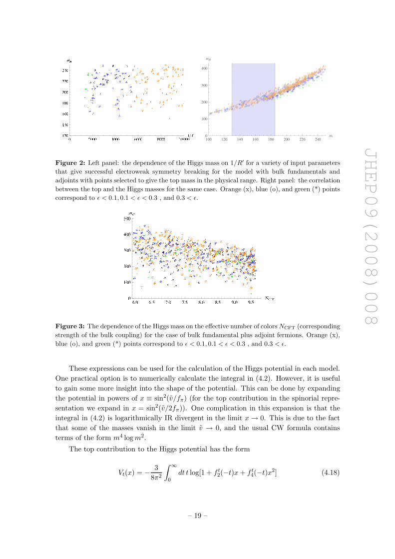
Figure 2: Left panel: the dependence of the Higgs mass on 1/R′ for a variety of input parameters
that give successful electroweak symmetry breaking for the model with bulk fundamentals and
adjoints with points selected to give the top mass in the physical range. Right panel: the correlation
between the top and the Higgs masses for the same case. Orange (x), blue (o), and green (*) points
correspond to ǫ < 0.1, 0.1 < ǫ < 0.3 , and 0.3 < ǫ.
Figure 3: The dependence of the Higgs mass on the effective number of colorsNCFT (corresponding
strength of the bulk coupling) for the case of bulk fundamental plus adjoint fermions. Orange (x),
blue (o), and green (*) points correspond to ǫ < 0.1, 0.1 < ǫ < 0.3 , and 0.3 < ǫ.
These expressions can be used for the calculation of the Higgs potential in each model.
One practical option is to numerically calculate the integral in (4.2). However, it is useful
to gain some more insight into the shape of the potential. This can be done by expanding
the potential in powers of x ≡ sin2(v/fπ) (for the top contribution in the spinorial repre-
sentation we expand in x = sin2(v/2fπ)). One complication in this expansion is that the
integral in (4.2) is logarithmically IR divergent in the limit x→ 0. This is due to the fact
that some of the masses vanish in the limit v → 0, and the usual CW formula contains
terms of the form m4 logm2.
The top contribution to the Higgs potential has the form
Vt(x) = − 3
8π2
∫ ∞
0dt t log[1 + f t
2(−t)x+ f t4(−t)x2] (4.18)
– 19 –

JHEP09(2008)008
For small x this can be expanded as
Vt(x) = at1x+ at
2x2 + nt
2x2 log
2ctx
Λ2+ O(x3) (4.19)
We defined the coefficient ct that captures the IR behavior of the form factors, namely
f t1(−t) ≈ −f t
2(−t) ≈ ct/t for t → 0, and it is related to the SM top quark mass by
m2t ≈ ctx. This coefficient can be read off from the top spectral function by replacing
Cc → 1, Sc → itR′(R′/R)−2cf−2c . We can then show that the general expression for the
coefficients in the expansion should be
at1 = − 3
8π2
∫ ∞
0dt tf t
2
at2 = − 3
16π2
[∫ ∞
0dt t
(
2f t4 − (f t
2)2 +
c2
Λ4 sinh2(t/Λ2)
)
− 3
2c2t
]
nt2 = − 3
16π2c2t (4.20)
The scale Λ is an IR regulator and it may take an arbitrary value. The expansion param-
eters depend on Λ in such a way that the dependence on the IR regulator cancels out at
order x2.
In the cases when the top contribution, dominates the minimum of the potential is
given by the approximate formula:
xm = − at1
2at2 + nt
2 + 2nt2 log(2cxm/Λ2)
(4.21)
In practice, however, the acceptable minimum with xm ≪ 1 occurs only for fine-tuned
values of the parameters such that at1 is much smaller than its natural value ∼ m2
t (R′)2/4π2.
In that case, the W and Z boson contributions can significantly shift the minimum, and
the acceptable EW breaking vacuum occurs for different c-parameters than without the
gauge contributions. The gauge contributions are calculated from
VW (x) =3
16π2
∫ ∞
0dt t log[1 + fW
2 (−t)x]
VZ(x) =3
32π2
∫ ∞
0dt t log[1 + fZ
2 (−t)x] (4.22)
and the expansion can be done analogously as for the top, by setting fW,Z4 = 0. In our
numerical studies we take the gauge contributions into account.
We turn to discussing the main features of the Higgs potential generated by the top,
bottom and gauge loops. We have scanned the parameter space to find self-consistent
combinations leading to realistic EWSB. In the scan we first choose the brane kinetic term
r, the bulk masses cq3and cd3
, the size of the brane masses mu, md, Mu, Md, the KK
scale 1/R′ and keep the hierarchy fixed at R/R′ = 10−16. We then determine v/fπ such
that the mW mass is reproduced and finally choose cu3such that the minimum of the
Coleman-Weinberg potential is really at this value of v/fπ.
– 20 –

JHEP09(2008)008
For the case of fundamental plus adjoint bulk fermions we do find plenty of realistic
values for the Higgs and the top masses, in agreement with the results of [31]. This is
illustrated in figure 2. Note however, that in order to fit the W-mass successfully with
a sufficiently small ǫ one is usually forced to introduce UV localized kinetic terms. The
dependence of the Higgs mass on the UV localized kinetic terms is illustrated in figure 3.
For our analysis of the flavor scales we are only selecting from the points that give a
satisfactory top with low values of ǫ.
However, there is a fine tuning reminiscent of the little hierarchy problem showing up:
if one fixes the mixing parameters mu,d, Mu,d and the bulk masses cq,d, then for given radii
R,R′ and for generic choices of the other parameters we have only a very narrow region in
the parameter cu that produces an ǫ which is phenomenologically acceptable (for example
0.1 < ǫ < 0.45). This suggests that in the interesting region with proper electroweak
symmetry breaking there will be a strong sensitivity of ǫ to the input parameters. This
was first pointed out in [30] and we find it to be a general property of all representations
studied in this paper. To illustrate this we show two examples of the dependence of ǫ on
cu in figure 4. The first one is a randomly chosen point where one has to adjust cu to a
high precision in order to find proper EWSB, while the second one corresponds to the best
case scenario that we could find after searching for regions where the tuning is milder. We
can see that the derivative of ǫ is very large in the first point, and even in the second point
it is still quite sizeable.
In order to quantify the tuning in these models we have calculated the local sensitivity
to the input parameters in the ranges given in section 5.3, for the regions with acceptable
electrowaek symmetry breaking only. We then define the local fine tuning as [32, 35]
t−1 = max
∣
∣
∣
∣
∂ log ǫ
∂ log ai
∣
∣
∣
∣
(4.23)
In this scan we have only included points where EWSB happens with a sufficiently
small S parameter and excluded all other points. The parameters ai were taken to be
cq3, cu3
, mu, Mu. We then estimate the average tuning for given ǫ by fitting the average of
t with a quadratic polynomial in ǫ. The best fit is approximately
t ∼ 1
4ǫ2 (4.24)
which qualitatively agrees with the ǫ2 estimate of [17] but is numerically somewhat stronger.
This implies that the average local tuning is a about half a percent for ǫ = 0.1, while about
5% for ǫ = 0.4. To verify those estimates we extended the parameter space to a large grid
in the parameters cq3, cu3
, mu, Mu and checked that the above fit for t = t(ǫ) remains a
conservative lower bound over all parameter space. These averages are shown as crosses in
figure 5 where each cross contains the average of about 200 points. Note however that one
can find restricted local areas in parameter space where the fine tuning is less severe than
the above quoted average.
For the spinorial representations we find that the bottom KK tower plays an important
role in electroweak symmetry breaking. Without including the bottom tower we could not
– 21 –

JHEP09(2008)008
Figure 4: The plots show the dependence of v/fπ on cu of the third generation for two sets of
parameters in the model with fundamentals and adjoints. The first example on the left shows a
generic point where there are only two narrow regions of cu that lead to an acceptable electroweak
breaking vacuum. The continuous line shows the result of the minimization of the full potential
and the dashed line shows our approximation for regions where sin v/fπ is small. In the left plot
for −0.46 <∼ cu3<∼ 0.46 the minimum of the potential is at v = πfπ/2, while for cu3
<∼ − 0.47 and
cu3>∼ 0.47 the minimum is at v = 0. In the case of v = πfπ/2, electroweak symmetry is maximally
broken mW = gf/2, whereas for v = 0, electroweak symmetry is unbroken (mW = 0). In both
cases there are massless fermions in the spectrum. For −0.47<∼ cu3<∼ − 0.46 and 0.46<∼ cu3
<∼ 0.47
there is a minimum at intermediate values of v/fπ, yet an additional tuning is required to arrive at
v/fπ ≪ 1. For v/fπ < 0.45 we find −0.464 < cu3< −0.462 and 0.464 < cu3
< 0.466. In this case
one needs to tune cu to more than a percent level to get successful electroweak symmetry breaking.
The right plot shows the same for carefully chosen values of the input parameters, where the local
tuning is more modest. In this best case scenario we can have a realistic electroweak symmetry
breaking minimum for the region −0.21 < cu3< −0.13 or 0.22 < cu3
< 0.31. The parameters
chosen for this plot are R′/R = 1016,1/R′ = 1.5TeV and cQ3= 0.42, cd3
= −0.56, mu = 5, md = 1,
Mu = 0, r = 1 (right: cQ3= 0.1, cd3
= −0.56, mu = 1, Mu = −0.5, r = 0.47).
Figure 5: This plot shows the local tuning t for the model with adjoints and fundamentals. The
orange line is a fit to a quadratic polynomial for which we find t ∼ 1
4ǫ2.
– 22 –

JHEP09(2008)008
Figure 6: Left panel: the dependence of the Higgs mass on 1/R′ for a variety of input parameters
in the model with spinors that give successful electroweak symmetry breaking with points selected
to give the top mass in the physical range. Right panel: the correlation between the top and the
Higgs masses. Orange (x), blue (o), and green (*) points correspond to ǫ < 0.3, 0.3 < ǫ < 0.4 , and
0.4 < ǫ.
find any point with a sufficiently heavy Higgs mass. Including the bottom improves the
situation because for the spinorial representation there is also a light KK mode in the
bottom sector.7 However, it is exactly this state that is responsible for the large shift in
the Zbb vertex. The fine tuning in the top sector is somewhat stronger for the spinorial
case than for the fundamental+adjoint discussed above. Once we impose the fine-tuning in
the input parameters of the theory, we still need to make sure that the Higgs is sufficiently
heavy. Most of the time the top is too heavy. The reason behind this is that there is a very
strong correlation between the Higgs and the top masses in this model. These correlations
between the Higgs mass and 1/R′ and mtop are summarized in figure 6.
4.1 Constraints from electroweak precision tests
Apart from yielding the correct electroweak breaking vacuum, phenomenologically accept-
able GHU models must pass stringent electroweak precision tests [35, 27]. Since SO(5)
models are endowed with custodial symmetry, there is no tree-level constraints from the T
parameter. The S parameter however is an issue. The expression for the S parameter (for
vanishing brane kinetic terms) is given by [17]
S = 4πv2
[
(∫ R′
R a)(∫ R′
R a−1)2 −∫ R′
R a(∫ R′
z a−1)2∫ R′
R a−1
]
≈ 3πv2R′2
2(4.25)
Demanding S < .2 yields the bound R′−1 > 1.2TeV. This implies that the lightest gauge
boson KK modes have masses ∼ 2.4R′−1 ∼ 3TeV.
Another potentially dangerous contributions to the electroweak observables are the
corrections to the ZbLbL coupling that is measured with the .25% accuracy. There are
two potential sources of deviations in the Zbb couplings: mixing of the zero mode fermions
7We thank Roberto Contino for discussions on this point.
– 23 –

JHEP09(2008)008
(after EWSB) with KK states of equal electric but different SU(2)L×U(1) charges, and
mixing among the gauge bosons.
We first estimate the contribution of the fermion mixing effect after EW breaking.
Since the b gains a mass after EWSB, in principle one can no longer use the zero mode
wave functions. Most of the time, these corrections are of order (mbR′)2, and so can be
safely ignored. However, in the spinorial model one encounters order (mtR′)2 corrections.
The leading effect of EWSB will be to twist the zero mode wave functions between the L
and R multiplets of a bulk spinor via the Wilson line matrix. The effect of this twisting
(for simplicity, we set Mu = Md = 0) will be that the left handed bottom quark will end
up partly living in the down-type component of χbcu. The reason why there is a component
in χbcu
(but not in χbcq
or χbcd) is that the UV brane boundary conditions only allow a non-
vanishing component in this this mode. This non-vanishing component in χbcu
will give the
leading correction to the Zbb vertex. The coupling of the zero mode of Z (in the limit it
is flat) is given by gZff ∼ (T3L − sin2 θQ). Since the electric charges of all components
that mix are the same the only correction comes from the deviation in the coupling to T3L,
which in our case is due to the fact that the χbcu
component couples to T3R and not to T3L.
So the relative deviation can be estimated to be (where s2 = 1 − c2 = sin2 v2f ).
δgZbL bL
gZbLbL
∼ sin2(v/2f)m2u
f2u
[
1f2
q+ m2
u
f2u
+m2
d
f2
d
] (4.26)
This expression can be related to the formula for the top mass, and so we find
δgZbb
gZbb
∼ (mtopR′)2
f2uf
2−u
∼ (mtopR′)2
(1 − 4c2u)(4.27)
For the range of interest R′ ∼ 1 − 2TeV and |cu| < 1/2 we will find a correction that is
always at least a percent, and cannot be removed. For the other two models the effect does
not occur due to the custodial protection proposed in ref. [18].
We move to the gauge contribution to the Zbb vertex. That correction can be calcu-
lated from the formula
δgZbLbL
gZbLbL
= m2Z
∫ R′
R(z/R)−2cq
−∫ z
Rz′ log(z′/R) +
T 3R − g2
g′2Y
T 3L − g2
g′2Y
(∫ z
Rz′ log(R′/R)
)
(4.28)
We know from the analysis of the Higgs potential that we need cq < 1/2. For generic
left and right quantum numbers of bL, the result is of order m2ZR
′2 log(R′/R), that is
enhanced by the large logarithm. This would lead to more stringent bounds than those
from the S parameter. However, in the models where bL is embedded in the bifundamental
representation with T 3L = T 3
R there is a cancellation of the large logs and the result is given
byδgZbLbL
gZbLbL
≈ m2ZR
′2
4
(
1 − 4
(3 − 2cq)2
)
(4.29)
This is below the experimental sensitivity even for R′ = 1TeV.
– 24 –

JHEP09(2008)008
5. Flavor in GHU
We begin our study of the flavor structure of GHU models. In this section we present a
detailed discussion for the model of section 3.2, with each SM generation embedded in two
fundamental and one adjoint SO(5) multiplet. The other two models lead to a very similar
flavor structure, and we will later comment on the differences.
5.1 Fermion masses and mixing
We start by discussing the zero modes before EW breaking produces their mass terms.
One difference with respect to the standard RS scenario is the presence of the IR boundary
mass terms. These do not give masses to the zero modes, but imply that the zero modes
are embedded in several bulk multiplets. In particular, the zero mode quark doublets qLare embedded in all Ψq,u,d in eq. (3.10), while the up-type quark singlets uR lives in Ψq,u.
On the other hand, the down-type quark singlets dR lives only in Ψd. We write
qq(x, z) → χqq(z)qL(x) qq(x, z) → χqu(z)qL(x) qd(x, z) → χqd(z)qL(x) (5.1)
ucu(x, z) → ψuc
u(z)uR(x) uc
q(x, z) → ψucq(z)uR(x) dr(x, z) → ψdr
(z)dR(x) (5.2)
Recall that we drop the generation index, and qL, uR, dR are understood to be three-
vectors in the generation space. The zero-mode profiles χ(z), ψ(z) are 3x3 matrices χq =
diag(χq1, χq2
, χq3) that determine how much of the zero mode resides in each 5D fermion.
Solving the equations of motion and the boundary conditions we find the left-handed
profiles:
χqq(z) =1√R′
( z
R
)2 ( z
R′
)−cq
fq
χqu(z) =1√R′
( z
R
)2 ( z
R′
)−cu
m†ufq
χqd(z) =
1√R′
( z
R
)2 ( z
R′
)−cd
m†dfq (5.3)
where fq = diag(f(cq1), f(cq2
), f(cq3)) and f(c) were defined in eq. (2.6). Similarly, the
zero mode profiles for the right handed up-type fields are given by
ψucu(z) =
1√R′
( z
R
)2 ( z
R′
)cu
f−u
ψucq(z) = − 1√
R′
( z
R
)2 ( z
R′
)cq
Muf−u, (5.4)
Finally, the down-type zero modes are contained only in the adjoints:
ψdr(z) =
1√R′
( z
R
)2 ( z
R′
)cd
f−d . (5.5)
The overall normalization has been chosen such that we recover the usual normalized zero
modes eq. (2.5) in the limit when the boundary masses are set to zero. In this form, our
profiles closely resemble the corresponding formulae in the standard RS set-up. However,
– 25 –

JHEP09(2008)008
in this basis, the kinetic terms for the zero modes are not diagonal. This kinetic mixing is
parameterized by the Hermitian 3 by 3 matrices
Kq = 1 + fqmuf−2u m†
ufq + fqmdf−2d m†
dfq,
Ku = 1 + f−uM†uf
−2−q Muf−u,
Kd = 1, (5.6)
For example, for the doublet zero modes the kinetic term is given by iqL(x)Kq∂/qL(x). The
kinetic mixing is inevitable in GHU models: since all the SM flavor mixing must originate
from non-diagonal terms in the boundary mass terms, at least the matrix Kq must be
non-diagonal. This is an important difference with respect to the original RS set-up that
will introduce additional contributions to flavor-violating processes.
In GHU, the fermion masses originate from the bulk kinetic terms ΨiDMΓMΨ, where
Dz → ∂z−ig5AazT
a and T a are the SO(5) generators appropriate for a given representation.
When Az acquires a vev it produces a mass term connecting the quarks living in the same
SO(5) multiplet. For the fundamental representation, the Wilson line marries the two up
quarks in the bifundamental to the singlet up quark:
(
R
z
)4 g∗v
2
√2z
R′ uc(u− u) (5.7)
while for the adjoint representation, it couples the triplets to the bifundamental, for exam-
ple(
R
z
)4 g∗v
2
√2z
R′ (dl − dr)dd (5.8)
Plugging in the zero mode profiles we find for the mass matrix (in the basis were the
kinetic terms are not diagonal)
mu =g∗v
2√
2fq(mu − Mu)f−u
md =g∗v
2√
2fqmdf−d (5.9)
To obtain the actual masses and mixing angles one needs to first diagonalize the kinetic
mixing terms and rescale the fields. We decompose Ka = VaNaV†a for a = q, u, d, where
N is a positive diagonal matrix and V a unitary matrix, and we define the corresponding
Hermitian matrix Ha = VaN−1/2a V †
a . The Hermitian rotation of the zero modes, qL →HqqL, uR → HuuR, brings the kinetic terms to the canonical form. The mass matrices
rotate into
mSMu =
g∗v
2√
2Hqfq(mu − Mu)f−uHu
mSMd =
g∗v
2√
2Hqfqmdf−d. (5.10)
In the next step we decompose, as usual, the up and down mass matrices as mSMu,d =
UL u,dmu,dU†R u,d, and we perform a unitary rotation of the zero mode quarks so as to
diagonalize the mass matrix, dL,R → UL,R ddL,R, uL,R → UL,R uuL,R .
– 26 –

JHEP09(2008)008
The flavor structure following from 5.10 is very similar to that of the ordinary RS model
with anarchic flavor structure, cf. (2.8). The main difference between (5.10) and (2.8) is
the appearance of the extra Hermitian matrices Ha that originate from the kinetic mixing.
Note that, since Na the eigenvalues of the kinetic mixing matrices (5.6), all entries of Na
are very close to 1 except maybe for the third generation. For this reason, the hierarchical
structure of the mass matrix will turn out to be very similar to that in RS.
The quark masses that follow from (5.10) are as usual, approximately equal to the
diagonal elements. They can be estimated by
mu ∼ g∗v
2√
2
(mu − M)fqf−u√
(
1 +f2
q m2u
f2u
+f2
q m2
d
f2
d
)
(
1 +f2
−uM2
f2−q
)
md ∼ g∗v
2√
2
mdfqf−d√
(
1 +f2
q m2u
f2u
+f2
q m2
d
f2
d
)
(5.11)
where mu,d, M here denotes the typical amplitude of the entries in the corresponding mass
matrix. As in the standard RS, the mass hierarchies are set by fq, f−u, f−d and g∗/2
plays the similar role to the Yukawa coupling Y∗. The coupling g∗ is however related to
the experimentally measured weak coupling, see eq. (3.2), and cannot be varied, unless
we consider large UV brane kinetic terms. Another difference is the dependence on the
boundary masses that enters both the numerator and the denominator. The latter may be
significantly different than 1 only when fx ∼ 1, which is the case for the third generation.
In that case mu,d, M saturate: further increasing it does not increase the mass.
We turn to discussing the mixing angles and how are they affected by the kinetic
mixing. Consider the doublet mixing matrix Kq. fq is hierarchical, fq1≪ fq2
≪ 1, fq3∼ 1,
while fu,d’s are all of order one (since it is f−u,d that sets the mass hierarchy). Thus,
Kq ∼ δij + m2fqifqj
, where we denote m2 = m2u + m2
d. It follows that Nq ∼ (1, 1, 1 + m2)
and (Vq)12 ∼ m2fq1fq2
, (Vq)13 ∼ m2fq1/(1 + m2), (Vq)23 ∼ m2fq2
/(1 + m2). At the end
of the day, the left hierarchy is set by the matrix fqHq (rather than fq as in RS) whose
diagonal elements are of the form
Hqfq ∼
fq1
fq2
fq3(1 + f2
q3m2)−1/2
, (5.12)
The off-diagonal terms in the above matrix are irrelevant for the following discussion. We
can see that the corrections coming from the kinetic mixing do not change the hierarchy
of fq. There are, of course, O(1) corrections in the actual numerical values of the f ’s that
are required to reproduce the mass and mixing hierarchies, but their orders of magnitude
are unchanged so that implementation of flavor hierarchies is analogous as in RS. The only
parametric difference between fq and eq. (5.12) is that the third eigenvalue gets suppressed
by 1/m as soon as m is larger than 1. We keep track of that effect because, as the study
of the Higgs potential shows, the interesting parameter space with successful electroweak
– 27 –

JHEP09(2008)008
breaking and the large enough top quark mass extends to m ∼ few. This parametric
dependence feeds into the left rotation that diagonalize the SM mass matrix,
(ULu,d)12 ∼ fq1
fq2
(ULu,d)13 ∼ fq1
fq3
(1 + f2q3m2)1/2 (ULu,d)23 ∼ fq2
fq3
(1 + f2q3m2)1/2 (5.13)
The consequence is that the relation between fq and the CKM angles is slightly modified,
(1 + m2)1/2fq1∼ λ3, (1 + m2)1/2fq1
∼ λ2, where λ is the Cabibbo angle.
By the same token,
Huf−u ∼
f−u1
f−u2
f−u3(1 + f2
−u3M2)−1/2
, (5.14)
and the elements of the right rotation matrix for the up-type quark are
(URu)12 ∼ f−u1
f−u2
(URu)13 ∼ f−u1
f−u3
(1 + f2−u3
M2)1/2 (URu)23 ∼ f−u2
f−u3
(1 + f2−u3
M2)1/2
(5.15)
Finally, the elements of the right rotation matrix for the down-type quark are not affected
by the kinetic mixing,
(URd)12 ∼ f−d1/f−d2
(URd)13 ∼ f−d1/f−d3
(URd)23 ∼ f−d2/f−d3
(5.16)
5.2 Flavor constraints
We are ready to evaluate the flavor constraints in the GHU models that originate from a
tree-level exchange of the KK gluons. To this end, we need to compute the couplings of
the SM down-type quarks to the lightest KK gluon,
gijL d
iLγµGµ(1)d
jL + gij
R diRγµGµ(1)d
jR (5.17)
As before, we introduce the diagonal matrix gx ≈ gs∗(− 1log R′/R + γ(cx)f2
x), x = q,−u,−d,that approximate the couplings of quarks in each 5D multiplets to the lightest KK gluon.
The complication inherent to the GHU models is that the zero mode quarks are contained
in several 5D multiplets. This is already one source of off-diagonal couplings. Furthermore,
on top of the unitary rotation that diagonalizes the SM mass matrix, the off-diagonal terms
are affected by the Hermitian rotation that diagonalizes the kinetic terms. At the end of
the day the couplings can be written as
gijL ≈
[
U †L dHq
(
gq + fqmuf−2u gum
†ufq + fqmdf
−2d gdm
†dfq
)
HqUL d
]
ij
gijR ≈
[
U †R dg−dUR d
]
ij(5.18)
Compared to the RS formula (2.16), the doublet quark off-diagonal couplings receive many
additional contributions. In spite of that, the RS-GIM mechanism is still at work, in the
– 28 –

JHEP09(2008)008
sense that the off-diagonal terms are always multiplied by the hierarchical matrix fq. The
flavor-changing couplings are proportional to
gdsL ∼ gs∗(1 + m2)fq1
fq2
gdbL ∼ gs∗
1 + m2
(1 + f2q3m2)1/2
fq1fq3
gsbL ∼ gs∗
1 + m2
(1 + f2q3m2)1/2
fq2fq3
(gR,d)ij ∼ gs∗f−dif−dj
(5.19)
We can now estimate the size of the FCNC four-fermion operators relevant for the for
the Kaon mixing. The LL operator is, just like in RS, suppressed by the CKM matrix
elements,
C1K ∼ 1
6M2G
g2s∗|V ∗
tsVtd|2f4q3
(1 + m2)2
(1 + f2q3m2)2
(5.20)
This bound has almost the same form as in the RS case, except for the last factor that
depends on m. In RS one usually takes fq3∼ 0.3 (that is cq3
close to one half) to further
suppress the LL operator. In the case at hand, using the approximate expression for the
top mass, we can relate (for f−u3∼ 1)
fq3
√
1 + m2
1 + f2q3m2
∼ 2√
2mt
g∗v
√1 + m2
√
1 + M2
mu − M(5.21)
Taking mu,d ∼ M ∼ 1 we can rewrite our estimate as
C1K ∼ 1
(5 · 104 TeV)2
(
3TeV
MG
)2
(5.22)
which shows that a 3TeV KK gluon satisfies the bound listed in table 2.
On the other hand, the LR contribution is
C4K = −3C5
K ∼ 1
M2G
g2s∗g2∗
8mdms
v2
1 + m2
m2d
(5.23)
where this time we related f ’s to down-type quark masses via fqif−di
∼ 2√
2mid/g∗vmd.
Again, this estimate is very similar as in the RS case, with Y∗ replaced by g∗/2. The
new parametric difference is the factor (1 + m2)/m2d, which can be traced back to the
kinetic mixing. This factor may enhance (but never suppress) the coefficient, if md < 1 or
mu > md. In consequence (when boundary kinetic terms are ignored),
C4K ∼ 1
(1.5 · 104 TeV)2
(
3TeV
MG
)2
(5.24)
The numbers refer to the case when the boundary kinetic terms at the TeV scale are small,
so that g∗ ∼ g log1/2(R′/R) ∼ 4, gs∗ ∼ gs log1/2(R′/R) ∼ 6. We can see that ΛImC4
Kis a
– 29 –

JHEP09(2008)008
Figure 7: Scan of the effective suppression scale of ImC1K (left panel) ImC4K (right panel) and in
the scenario with adjoint and fundamental bulk fields. In the left panel points with mu > 3.5 are
red (*) and points with mu < 1.5 are black (+). All the points give the correct low-energy spectrum
but most of the points with mG < 30TeV fail to satisfy the ImC4K bound of Λ > 1.6 · 105 TeV.
The blue line is a linear fit of the MG dependence.
Figure 8: Scan of the effective suppression scale of |C4
Bd| (left panel) |C4
Bs| (right panel) and in
the scenario with adjoint and fundamental bulk fields. All the points give the correct low-energy
spectrum and points with mG > 5TeV mostly satisfy the bounds. The blue lines are linear fits of
the MG dependence.
factor of ∼ 11 too small for a 3TeV KK gluon. To satisfy the bound ΛImC4
K> 16 · 104 TeV
(see table 2) would require a KK scale of about 33 TeV.
As in RS, we can change this estimate by playing with the boundary kinetic terms for
SU(2)L and SU(3)C . Assuming a large bare UV coupling (small brane kinetic term) for
SU(3)c and including the one-loop QCD running we can decrease gs∗, thus relaxing the
bound by a factor of two. On the other hand, we could make the coupling g∗ larger by
adding a large brane kinetic term for SU(2)L, that is to pick r > 1. In the best of all
worlds, assuming gs∗ ∼ 3 and g∗ ∼ 4π (the latter implies lack of perturbative control over
the Higgs sector) we could lower the bound down to 5 TeV. In a calculable framework it is
not possible to lower the bound below 10 TeV. These estimates demonstrate that the GHU
framework with fully anarchic flavor is not a plausible scenario.
– 30 –

JHEP09(2008)008
5.3 Numerical scan
We have verified the above estimates of the flavor bounds by an extensive numerical scan
over the parameter space of the model. Our first aim is to find realistic electro-weak
symmetry breaking minima of the effective potential. We are only interested in points
with a sizable gap between the EW scale and the scale of the KK modes (v/fπ <∼ 0.3).
The parameters related by EWSB are: the bulk masses of the third generation cq3,cu3
,cd3,
the size of the brane masses mu, md, Mu, Md, the KK scale 1/R′. We keep the hierarchy
R/R′ = 10−16 fixed. Contrary to the RS case, we are not free to pick any combination,
since most choices do not lead to EWSB satisfying our criteria. As we have discussed, v/fπ
is very sensitive to qq3, cu3
, see e.g. figure 4. We therefore first randomly generate a set of
parameters with cq3∈ [0.2, 0.48], 1/R′ ∈ [900, 12500] GeV, c−d3
= −0.55, |mu| ∈ [0.5, 5],
|md| ∈ [0.5, 2], and r ∈ [0, 0.8]. (For simplicity, we have set Mu = Md = 0). Knowing
R,R′ and r, we determine v/fπ from the condition to reproduce mW , see (3.5). We then
find a cu3such that the minimum of the potential really is at the value of v/fπ specified
before. Finally, we want the theory to be calculable, which puts an upper bound on the
bulk SO(5) coupling g∗. This can be equivalently expressed as a bound on the number of
colors of the dual CFT, see eq. (3.1), and we require NCFT >∼ 5.
The next step is to calculate the SM masses, mixing angles and KK FCNCs. Given
the size of cq3,cu3
,cd3and of mu and md we can determine the bulk masses of the first
two generations. First, cq1and cq2
are fixed since left rotations (5.13) need to have the
same hierarchy as the CKM. The remaining bulk masses cu1,2,cd1,2
can be fixed using (2.13)
requiring the mass eigenvalues to match the SM at TeV scales.
Now we randomly generate complex 3 × 3 matrices mu, md with eigenvalues approxi-
mately of the size as those used in the calculation of the potential above. Using (5.10) we
then calculate the effective mass matrices mSMu,d . These mass matrices only approximately
reproduce the SM. In order to have a completely realistic set of parameters we need to
parameterize the deviation from the SM and reject those mu,d which deviate too much.
For this purpose we have defined matrix norms that measure the distance between the
generated and the physical values at 3 TeV. We calculate the distance between
• The mass eigenvalues to the the SM running masses at 3TeV, see table. 1.
• The moduli of the generated CKM to
|VCKM| ≈
0.97 0.226 0.0035
0.226 0.97 0.04
0.008 0.04 1
, (5.25)
which we took from a recent tree level determination [36].
• The amount of CP violation to the SM Jarlskog invariant [37]
J ≈ 3 · 10−5 (5.26)
We finally accept only those random matrices mu,d for which the maximal relative distance
of any constraint is below 30%.
– 31 –

JHEP09(2008)008
The results of the scan are displayed in figure 7. Most of the points with mG < 30 TeV
fail to satisfy the ImC4K bound of Λ > 1.6 · 105 TeV, in agreement with our analytical
estimates. Just like in the RS case this bound is somewhat dependent on the assumption
that one makes on the boundary kinetic terms for the gluon. For the two extreme cases
the numerical values for the supression scales are the following. In the worst case when the
theory is barely perturbative, the bound is enhanced to about 54 TeV, while in the best
case, with no bare brane kinetic terms to bound is reduced to about 17 TeV. We conclude
that the flavor constraints on the warped models with a pseudo-Goldstone Higgs are even
stronger that that in the standard RS with a TeV brane localized Higgs.
In the remainder of this section we summarize the flavor constraints for the other two
GHU models considered in this paper. The short summary is that in none of the models
is the RS flavor bound relaxed, but rather strengthened.
5.4 Fermions in the spinorial
For the model with each generation of the SM fermions embedded in 3 SO(5) spinors
the parameter space includes an additional boundary mass matrix Md that introduces the
kinetic mixing also to the d-singlet quark sector. The kinetic mixing matrices are given by
Kq = 1 + fqmuf−2u m†
ufq + fqmdf−2d m†
dfq,
Ku = 1 + f−uM†uf
−2−q Muf−u,
Kd = 1 + f−dM†df
−2−q Mdf−d, (5.27)
The SM up and down mass matrix take the form
mSMu,d =
g∗v
4Hqfq(mu,d − Mu,d)f−u,dHu,d. (5.28)
There is an additional factor of 1/√
2 that is a group theoretical factor of the spinorial
SO(5) representation. The kinetic mixing induced by Md feeds into the right-rotation
unitary matrix for the down quarks
(URd)12 ∼ f−d1
f−d2
(URd)13 ∼ f−d1
f−d3
(1 + f2−d3
M2)1/2 (URd)23 ∼ f−d2
f−d3
(1 + f2−d3
M2)1/2
(5.29)
but the effect is negligible (unless M is very large) because f−d3≪ 1 to account for
mb/mt ≪ 1. The only difference in flavor constraints is the consequence of the 1/√
2 factor
in the SM mass matrix, which makes the LR flavor bounds a factor of√
2 more stringent.
5.5 Fermions in four fundamentals
The model with four fundamental representation per generation contains yet another ma-
trix θ that is a source of flavor violation. The kinetic mixing matrices are given by
Kq = 1 + fqu(R′/R)cqu θ†(R′/R)−cqdf−2qd
(R′/R)−cqd θ(R′/R)cqufqu + fqum†uf
−2u mufqu
+fqu(R′/R)cqu θ†(R′/R)−cqd mdf−2d m†
d(R′/R)−cqd θ(R′/R)cqufqu,
Ku = 1 + f−uM†uf
−2−qu
Muf−u,
Kd = 1 + f−dM†df
−2−qd
Mdf−d, (5.30)
– 32 –

JHEP09(2008)008
while the mass terms are
mSMu =
g∗v
2√
2Hqfqu(mu − Mu)f−uHu
mSMd =
g∗v
2√
2Hqfqu(R′/R)cqu θ†(R′/R)−cqd (md − Md)f−dHd (5.31)
There are several new possible flavor effects here. First of all, the mixing matrix θ shows,
and it is accompanied by the large factor (R′/R)cqu on the outside. This factor perfectly
counteracts the hierarchical suppression generated by the matrix fq. In consequence, as
long as θ is an arbitrary anarchic matrix, we definitely lose the RS hierarchic structure of
the fermion mass matrix. The origin of this is easy to understand. Here we have two copies
of the left handed doublets, and we are removing one combination with an additional right
handed doublet on the UV brane. If the matrix θ is anarchic, then we introduce a large
flavor violating effect into the elementary sector, that is unsuppressed by the mixing of
elementary and composite states.
In order for the UV physics to maintain an SU(3)Q flavor symmetry for the doublets
we need to assume that θ is, to a good approximation, proportional to the unit matrix.
In the following we set θ → Θ13x3 in all expressions, where Θ is a c-number. This is
in fact a similar assumption as the one implicitly makes in RS and the other two GHU
models: the elementary sector is flavor symmetric (that is there are no large flavor violating
kinetic mixing terms on the Planck brane), and only the CFT gives rise to flavor violations.
With this ansatz, the flavor structure becomes very similar to that in the spinorial model.
There is still another new effect, however, which is the presence of two sets of cq. As a
consequence, in the expression for mSMu,d the left hierarchy is not set by the same functions:
for the up-type masses it is set by fcquwhile for the down-type by fcqu
(R′/R)cqu−cqd . This
effect can be used as an alternative way to explain the large isosping breaking in the third
generation. Instead of taking f−d3≪ 1, that is assuming bR is mostly elementary, we can
choose f−d3∼ 1 and cq3
u< cq3
dto obtain mb/mt ≪ 1. Unfortunately, this new avenue does
not seem to lead to suppressing dangerous four-fermion operators. The coefficients C4K can
be estimated as
C4K ∼ (R′/R)
(cq1d−cq1
)+(cq2d−cq2
) 1
M2G
g2s∗g2∗
8mdms
v2
1 + m2
m2d
(5.32)
where cqi= min(cqi
u, cqi
d). For c
q1,2u
< cq1,2d
we are able to enhance the coefficient C4K , but
it’s not exactly what we want.
6. Conclusion
In this paper we studied flavor physics in the framework of 5D warped GHU models that
provide a dual realization of a composite pseudo-Goldstone Higgs. This is an extension of
the standard RS scenario, that makes the electroweak symmetry breaking dynamical and
fully calculable.
The flavor structure of GHU models turns out to be quite similar to that in RS. The
hierarchical structure of the quark masses and the CKM matrix appears as a consequence
– 33 –

JHEP09(2008)008
of different localization of zero modes in the extra dimension. The RS-GIM mechanism
is operating, in the sense that the coefficients of effective four-fermion ∆F = 2 operators
induced by the tree-level KK mode exchange are suppressed by the small off-diagonal CKM
matrix elements (LL operators), or by the light quark masses (LR operators).
The GHU models introduce, however, new contributions to flavor violation that are
of the same order of magnitude as those in RS. The reason is that the larger set of local
symmetries (that is crucial to realize the Higgs as a pseudo-Goldstone boson) imply a
different realization of the zero-mode fermionic sector. In particular, the zero modes must
be embedded in more than one bulk multiplet. We call it the kinetic mixing because in
the original flavor basis in 5D it shows up as the generation mixing via the zero modes
kinetic terms. This effect is controlled by the IR boundary masses - the same Lagrangian
parameters that control also the mass matrix. The kinetic mixing feeds into the effective
four-fermion ∆F = 2 operators, parametrically enhancing its coefficients by a factor of few.
Just like in RS, the strongest bound on the KK scale comes from the imaginary part
of the LR (sd)2 operator, that affects CP violation in the kaon sector. We find that for
anarchic boundary mass matrices, the generic bounds on the lightest KK gluon mass is of
order 30TeV. Such a large KK scale of course undermines the motivations for the GHU
models. This implies that GHU does not make sense without additional flavor symmetries.
There are several ways one could suppress the dangerous FCNC contributions (apart from
assuming accidental cancelations). For example in the models of [39] one imposes a bulk
flavor symmetry, and all mixing originates from Planck brane localized kinetic mixing
terms. As a result one can construct models where all tree-level FCNC’s are absent (a
genuine GIM mechanism), but of course in this case one gives up on the explanation of
the fermion mass hierarchy. A recent proposal suggests to truncate the bulk at a scale
of about 103 TeV which softens the flavor problem by effectively reducing gs∗ [41]. The
obvious price to pay is giving up on an explanation for the hierarchy between weak and
Planck scale. An intermediate solution could be to try to construct flavor models that do
explain both hierarchies, but have some partial flavor symmetries left over [25, 40]. One
possible ansatz that would alleviate the constraints while still giving rise to the hierarchies
would be to assume that the boundary masses in the down sector md, Md are proportional
to the unit matrix, so that all the CKM mixing originate from non-diagonal elements in
mu, Mu. This suppresses the right rotation matrix UR d, so that the LR operator is also
suppressed.
Acknowledgments
We would like to thank Kaustubh Agashe, Roberto Contino, Christophe Grojean, Sebastian
Jager, Gilad Perez, Jose Santiago, Martin Schmaltz, Luca Silvestrini, and Carlos Wagner
for useful discussions. We are grateful to Kaustubh Agashe, Roberto Contino and Gilad
Perez for important comments on the manuscript. The research of C.C. and A.W. is
supported in part by the NSF grant PHY-0355005 at Cornell and PHY05-51164 at the
KITP. A.F. is partially supported by the European Community Contract MRTN-CT-2004-
503369 for the years 2004–2008.
– 34 –

JHEP09(2008)008
A. KK gluon sums
In this appendix we present analytical formulas that allow one to include the contribution of
the entire KK gluon tower to the effective four-fermion operators. We start with couplings
of the n-th KK gluon to the quark eigenstates
gijL,nq
iLγµG
µ(n)qjL + gij
R,nqiRγµG
µ(n)qjR (A.1)
The couplings are given by
gijL,n = gs∗R
1/2
∫ R′
Rfn(z)hij
L (z) gijR,n = gs∗R
1/2
∫ R′
Rfn(z)hij
R(z) (A.2)
Above, a(z) is the warp factor (that we keep arbitrary here), fn(z) is the profile of the
n-th KK gluon, and g5 is the dimensionful bulk coupling of SU(3) color. For vanishing
brane kinetic terms, the SM strong coupling is given by g2s = g2
s∗R/L, where L =∫ R′
R a(z).
The quark bilinear profiles hijL,R(z) are 3x3 matrices in the mass eigenstate basis. They are
related to the fermionic profiles:
hL(z) = a4(z)V †L
∑
a
χ†qa
(z)χqa(z)VL hR(z) = a4(z)V †R
∑
a
ψ†qa
(z)ψqa(z)VR (A.3)
where the sum goes over all bulk multiplets in which the quark eigenstates is embedded,
and VL,R collectively denote all Hermitian or unitary rotations that relate the original
flavor basis to the mass eigenstate basis. By orthogonality, the bilinear profiles satisfy∫ R′
R hijL,R = δij .
The coefficients of the effective four-fermion operators are set by the sums of the form
Σij,klLR =
∞∑
n=1
gijL,ng
klR,n
m2n
(A.4)
Strangely enough, with the help of the methods of ref. [42] the sum can be evaluated for a
general warp factor (even though there is no closed expression for particular mn and gn).
The strategy is to 1) insert the integral expression for the couplings into the sum, 2) use
the integrated equation of motion for fn(z), and 3) use the completeness relation for fn(z).
When the smoke clears, one is left with
Σij,klLR = g2
s
[
L
∫ R′
Ra−1(z)(
∫ z
Rhij
L (z′))(
∫ z
Rhkl
R (z′)) (A.5)
+δij
∫ R′
Rhkl
R (z)
∫ z
Ra−1(z′)
∫ z′
Ra(z′′) + δkl
∫ R′
Rhij
L (z)
∫ z
Ra−1(z′)
∫ z′
Ra(z′′)
]
−g2sδ
ijδkl
[
∫ R′
Ra−1(z′)
∫ z′
Ra(z′′) + L−1
∫ R′
Ra(z)
∫ z
Ra−1(z′)
∫ z′
Ra(z′′)
]
The result is quite complicated, but it simplifies considerably for flavor changing sums,
which are of primary interest here:
Σij,klLR = g2
sL
∫ R′
Ra−1(z)
(
∫ R′
zhij
L (z′)
)(
∫ R′
zhkl
R (z′)
)
i 6= j k 6= l (A.6)
– 35 –
JHEP09(2008)008
Thus, the whole sum is expressed by simple integrals of the warp factor and the fermion
profiles. In particular, for AdS geometry we take a(z) = R/z, and the fermionic profiles
from eq. (2.5). The inverse of the AdS warp factor is sharply peaked towards IR. Therefore
the integrals depend mainly on the IR value of the fermionic profiles, that also sets the
fermion masses and mixing angles. This is the origin of the RS-GIM mechanism.
The coefficients of the operators relevant for the kaon sector are given by
C1K =1
6g2s log(R′/R)
∫ R′
Rz
(
∫ R′
zhsd
L (z′)
)(
∫ R′
zhsd
L (z′)
)
C4K = −g2s log(R′/R)
∫ R′
Rz
(
∫ R′
zhsd
L (z′)
)(
∫ R′
zhsd
R (z′)
)
C5K = −1
3C4K (A.7)
In RS, the bilinear profiles of the down-type quarks are given by
hL,d(z) = R′−1U †L d
(
R′
z
)2cq
f2qUL d
hR,d(z) = R′−1U †R d
(
R′
z
)−2cd
f2−dUR d (A.8)
Here, the non-diagonal elements are only due to the left and right unitary rotations that
diagonalize the SM mass matrix.
For the GHU model with two fundamentals and an adjoint, the right-handed down-
quark bilinear profile remains the same, but the left-handed one becomes more complicated
due to the kinetic mixing:
hL,d(z) = R′−1U †L dHq
[
(
R′
z
)2cq
f2q + fqmu
(
R′
z
)2cu
m†ufq+fqmd
(
R′
z
)2cd
m†dfq
]
HqUL d.
(A.9)
This time there are new sources of off-diagonal terms: the boundary masses m and the
Hermitian rotations H.
B. SO(5) generators
B.1 Spinorial
The smallest SO(5) representation is the 4 spinorial. The generators in a convenient basis:
T aL =
1
2
[
σa 0
0 0
]
T aR =
1
2
[
0 0
0 σa
]
(B.1)
T aC =
i
2√
2
[
0 σa
−σa 0
]
T 4C =
1
2√
2
[
0 1
1 0
]
(B.2)
– 36 –

JHEP09(2008)008
T aL and T a
R generate the SO(4) ≡ SU(2)L×SU(2)R subgroup of SO(5) and T aC are the coset
generators. The T3 generators of the SU(2)L ×SU(2)R subgroup are diagonal in this basis.
This makes transparent how the SU(2)L × SU(2)R quantum numbers are embedded in 4:
Ψ =
q+0
q−0
q0+q0−
4 = (2,1) ⊕ (1,2) (B.3)
where ± stands for ±1/2. The Wilson-line exponential ei√
2hT 4
C rotates q±0 into q0± and
vice-versa:
q±0 → cos(h/2)q±0 + i sin(h/2)q0±
q0± → i sin(h/2)q0± + cos(h/2)q±0 (B.4)
B.2 Fundamental
The 10 generators of the fundamental representation in an inconvenient basis:
T aL,ij = − i
2
[
1
2ǫabc(δb
i δcj − δb
jδci ) + (δa
i δ4j − δa
j δ4i )
]
a = 1 . . . 3
T aR,ij = − i
2
[
1
2ǫabc(δb
i δcj − δb
jδci ) − (δa
i δ4j − δa
j δ4i )
]
a = 1 . . . 3
T aC,ij = − i√
2
[
δai δ
5j − δa
j δ5i )]
a = 1 . . . 4 (B.5)
The generators are normalized as TrTαT β = δαβ . The T3 generators of SU(2)L × SU(2)Rare non-diagonal in this basis. The quantum numbers of the 5-vector components can be
found as:
Q =1√2
q++ + q−−iq++ − iq−−q+− + q−+
iq+− − iq−+√2q00
5 = (2,2) ⊕ (1,1) (B.6)
The Wilson-line transformation exp(i√
2hT 4C) rotates (q+−, q−+, q00) into one another:
q+− → 1 + cos(h)
2q+− +
1 − cos(h)
2q−+ − i
sin(h)√2q00
q−+ → 1 − cos(h)
2q+− +
1 + cos(h)
2q−+ + i
sin(h)√2q00
q00 → −isin(h)√2q+− + i
sin(h)√2q−+ + cos(h)q00 (B.7)
B.3 Adjoint
The antisymmetric tensor Φ transforms as Φ → ΩΦΩT . We can represent the tensor as:
Φ = ΦaLT
aL + Φa
RTaR + Φa
CTac (B.8)
– 37 –

JHEP09(2008)008
where T are SO(5) generators in the fundamental representation. The SO(5) commutation
relations
[T aL, T
bL] = iǫabcT c
L [T aR, T
bR] = iǫabcT c
R [T aL, T
bR] = 0 (B.9)
[T aC , T
bC ] =
i
2ǫabc(T c
L + T cR) [T a
C , T4C ] =
i
2(T a
L − T aR) (B.10)
[T aL,R, T
bC ] =
i
2
(
ǫabcT cC ± δabT 4
C
)
[T aL,R, T
4C ] = ∓ i
2T a
C (B.11)
imply that ΦL is an SU(2)L triplet, ΦR is an SU(2)R triplet and ΦC is an SU(2)L ×SU(2)Rbifundamental, and the embedding of the quantum numbers is
(3,1) : Φ1L ± iΦ2
L → (±1, 0) Φ3L → (0, 0) (B.12)
(1,3) : Φ1R ± iΦ2
R → (0,±1) Φ3R → (0, 0) (B.13)
(2,2) : Φ1C ± iΦ2
C → (±1/2,±1/2) Φ3C ± iΦ4
C → (±1/2,∓1/2) (B.14)
10 = (3,1) ⊕ (1,3) ⊕ (2,2) (B.15)
The Wilson-line transformation rotates the axial combination of the left and right triplets
into the bifundamental
ΦaL + Φa
R√2
→ ΦaL + Φa
R√2
ΦaL − Φa
R√2
→ ΦaL − Φa
R√2
cos(h) + ΦaC sin(h)
ΦaC → −Φa
L − ΦaR√
2sin(h) + Φa
C cos(h) (B.16)
References
[1] L. Randall and R. Sundrum, A large mass hierarchy from a small extra dimension, Phys.
Rev. Lett. 83 (1999) 3370 [hep-ph/9905221].
[2] H. Davoudiasl, J.L. Hewett and T.G. Rizzo, Bulk gauge fields in the Randall-Sundrum model,
Phys. Lett. B 473 (2000) 43 [hep-ph/9911262];
A. Pomarol, Gauge bosons in a five-dimensional theory with localized gravity, Phys. Lett. B
486 (2000) 153 [hep-ph/9911294].
[3] Y. Grossman and M. Neubert, Neutrino masses and mixings in non-factorizable geometry,
Phys. Lett. B 474 (2000) 361 [hep-ph/9912408].
[4] T. Gherghetta and A. Pomarol, Bulk fields and supersymmetry in a slice of AdS, Nucl. Phys.
B 586 (2000) 141 [hep-ph/0003129].
[5] S.J. Huber, Flavor violation and warped geometry, Nucl. Phys. B 666 (2003) 269
[hep-ph/0303183].
[6] K. Agashe, G. Perez and A. Soni, Flavor structure of warped extra dimension models, Phys.
Rev. D 71 (2005) 016002 [hep-ph/0408134].
[7] K. Agashe, M. Papucci, G. Perez and D. Pirjol, Next to minimal flavor violation,
hep-ph/0509117.
– 38 –
JHEP09(2008)008
[8] G. Burdman, Constraints on the bulk standard model in the Randall-Sundrum scenario, Phys.
Rev. D 66 (2002) 076003 [hep-ph/0205329]; Flavor violation in warped extra dimensions and
CP asymmetries in B decays, Phys. Lett. B 590 (2004) 86 [hep-ph/0310144].
[9] S. Davidson, G. Isidori and S. Uhlig, Solving the flavour problem with hierarchical fermion
wave functions, Phys. Lett. B 663 (2008) 73 [arXiv:0711.3376].
[10] K. Agashe et al., LHC signals for warped electroweak neutral gauge bosons, Phys. Rev. D 76
(2007) 115015 [arXiv:0709.0007].
[11] UTfit collaboration, M. Bona et al., Model-independent constraints on ∆F = 2 operators
and the scale of new physics, JHEP 03 (2008) 049 [arXiv:0707.0636].
[12] C. Csaki, C. Grojean, H. Murayama, L. Pilo and J. Terning, Gauge theories on an interval:
unitarity without a Higgs, Phys. Rev. D 69 (2004) 055006 [hep-ph/0305237];
C. Csaki, C. Grojean, L. Pilo and J. Terning, Towards a realistic model of Higgsless
electroweak symmetry breaking, Phys. Rev. Lett. 92 (2004) 101802 [hep-ph/0308038].
[13] D.B. Kaplan and H. Georgi, SU(2) × U(1) breaking by vacuum misalignment, Phys. Lett. B
136 (1984) 183.
[14] N. Arkani-Hamed, A.G. Cohen, E. Katz and A.E. Nelson, The littlest Higgs, JHEP 07 (2002)
034 [hep-ph/0206021].
[15] N.S. Manton, A New Six-Dimensional Approach to the Weinberg-Salam Model, Nucl. Phys.
B 158 (1979) 141;
Y. Hosotani, Dynamical mass generation by compact extra dimensions, Phys. Lett. B 126
(1983) 309; Dynamics of nonintegrable phases and gauge symmetry breaking, Ann. Phys.
(NY) 190 (1989) 233.
[16] R. Contino, Y. Nomura and A. Pomarol, Higgs as a holographic pseudo-Goldstone boson,
Nucl. Phys. B 671 (2003) 148 [hep-ph/0306259].
[17] K. Agashe, R. Contino and A. Pomarol, The minimal composite Higgs model, Nucl. Phys. B
719 (2005) 165 [hep-ph/0412089].
[18] K. Agashe, R. Contino, L. Da Rold and A. Pomarol, A custodial symmetry for Zbb, Phys.
Lett. B 641 (2006) 62 [hep-ph/0605341].
[19] S.J. Huber and Q. Shafi, Fermion masses, mixings and proton decay in a Randall-Sundrum
model, Phys. Lett. B 498 (2001) 256 [hep-ph/0010195].
[20] N. Arkani-Hamed and M. Schmaltz, Hierarchies without symmetries from extra dimensions,
Phys. Rev. D 61 (2000) 033005 [hep-ph/9903417].
[21] K. Agashe, A. Delgado, M.J. May and R. Sundrum, RS1, custodial isospin and precision
tests, JHEP 08 (2003) 050 [hep-ph/0308036].
[22] Particle Data Group collaboration, W.M. Yao et al., Review of particle physics, J. Phys.
G 33 (2006) 1.
[23] J.A. Bagger, K.T. Matchev and R.-J. Zhang, QCD corrections to flavor-changing neutral
currents in the supersymmetric standard model, Phys. Lett. B 412 (1997) 77
[hep-ph/9707225];
M. Ciuchini et al., Next-to-leading order QCD corrections to ∆(F ) = 2 effective hamiltonians,
Nucl. Phys. B 523 (1998) 501 [hep-ph/9711402];
A.J. Buras, S. Jager and J. Urban, Master formulae for ∆(F ) = 2 NLO-QCD factors in the
standard model and beyond, Nucl. Phys. B 605 (2001) 600 [hep-ph/0102316].
– 39 –
JHEP09(2008)008
[24] G. Moreau and J.I. Silva-Marcos, Flavour physics of the RS model with KK masses reachable
at LHC, JHEP 03 (2006) 090 [hep-ph/0602155].
[25] A.L. Fitzpatrick, G. Perez and L. Randall, Flavor from minimal flavor violation & a viable
Randall-Sundrum model, arXiv:0710.1869.
[26] K.-y. Oda and A. Weiler, Wilson lines in warped space: dynamical symmetry breaking and
restoration, Phys. Lett. B 606 (2005) 408 [hep-ph/0410061].
[27] M.S. Carena, E. Ponton, J. Santiago and C.E.M. Wagner, Electroweak constraints on warped
models with custodial symmetry, Phys. Rev. D 76 (2007) 035006 [hep-ph/0701055].
[28] R. Contino, L. Da Rold and A. Pomarol, Light custodians in natural composite Higgs models,
Phys. Rev. D 75 (2007) 055014 [hep-ph/0612048].
[29] A. Falkowski, S. Pokorski and J.P. Roberts, Modelling strong interactions and longitudinally
polarized vector boson scattering, JHEP 12 (2007) 063 [arXiv:0705.4653].
[30] G. Panico, E. Ponton, J. Santiago and M. Serone, Dark matter and electroweak symmetry
breaking in models with warped extra dimensions, Phys. Rev. D 77 (2008) 115012
[arXiv:0801.1645].
[31] A.D. Medina, N.R. Shah and C.E.M. Wagner, Gauge-Higgs unification and radiative
electroweak symmetry breaking in warped extra dimensions, Phys. Rev. D 76 (2007) 095010
[arXiv:0706.1281].
[32] R. Barbieri and G.F. Giudice, Upper bounds on supersymmetric particle masses, Nucl. Phys.
B 306 (1988) 63.
[33] G.W. Anderson and D.J. Castano, Measures of fine tuning, Phys. Lett. B 347 (1995) 300
[hep-ph/9409419].
[34] A. Falkowski, About the holographic pseudo-Goldstone boson, Phys. Rev. D 75 (2007) 025017
[hep-ph/0610336]; Pseudo-goldstone Higgs from five dimensions, arXiv:0710.4050.
[35] K. Agashe and R. Contino, The minimal composite Higgs model and electroweak precision
tests, Nucl. Phys. B 742 (2006) 59 [hep-ph/0510164].
[36] UTfit collaboration, M. Bona et al., The UTfit collaboration report on the unitarity triangle
beyond the standard model: spring 2006, Phys. Rev. Lett. 97 (2006) 151803
[hep-ph/0605213].
[37] C. Jarlskog, Commutator of the quark mass matrices in the standard electroweak model and a
measure of maximal CP-violation, Phys. Rev. Lett. 55 (1985) 1039.
[38] L. Randall and M.D. Schwartz, Quantum field theory and unification in AdS5, JHEP 11
(2001) 003 [hep-th/0108114];
W.D. Goldberger and I.Z. Rothstein, High energy field theory in truncated AdS backgrounds,
Phys. Rev. Lett. 89 (2002) 131601 [hep-th/0204160];
W.D. Goldberger and I.Z. Rothstein, Effective field theory and unification in AdS
backgrounds, Phys. Rev. D 68 (2003) 125011 [hep-th/0208060]; Systematics of coupling
flows in AdS backgrounds, Phys. Rev. D 68 (2003) 125012 [hep-ph/0303158];
K.-W. Choi and I.-W. Kim, One loop gauge couplings in AdS5, Phys. Rev. D 67 (2003)
045005 [hep-th/0208071];
K. Agashe, A. Delgado and R. Sundrum, Gauge coupling renormalization in RS1, Nucl.
Phys. B 643 (2002) 172 [hep-ph/0206099]; Grand unification in RS1, Ann. Phys. (NY) 304
(2003) 145 [hep-ph/0212028];
– 40 –

JHEP09(2008)008
R. Contino, P. Creminelli and E. Trincherini, Holographic evolution of gauge couplings, JHEP
10 (2002) 029 [hep-th/0208002].
[39] G. Cacciapaglia et al., A GIM mechanism from extra dimensions, JHEP 04 (2008) 006
[arXiv:0709.1714].
[40] C. Csaki, Y. Grossman, G. Perez, Z. Surujon and A. Weiler, work in progress.
[41] H. Davoudiasl, G. Perez and A. Soni, The little Randall-Sundrum model at the Large Hadron
Collider, Phys. Lett. B 665 (2008) 67 [arXiv:0802.0203].
[42] J. Hirn and V. Sanz, (Not) summing over Kaluza-Kleins, Phys. Rev. D 76 (2007) 044022
[hep-ph/0702005].
– 41 –
![Higgs Mechanism at Finite Chemical Potential with Type-II Nambu-Goldstone Boson Based on arXiv:1102.4145v2 [hep-ph] Yusuke Hama (Univ. Tokyo) Tetsuo Hatsuda](https://img.dokumen.tips/doc/110x75/56649ed85503460f94be6733/higgs-mechanism-at-finite-chemical-potential-with-type-ii-nambu-goldstone-boson.jpg)


![Higgs Mechanism at Finite Chemical Potential with Type-II ...€¦ · Higgs Mechanism at Finite Chemical Potential with Type-II Nambu-Goldstone Boson Based on arXiv:1102.4145v2 [hep-ph]](https://img.dokumen.tips/doc/110x75/5ec11d8f7d70e4118c52cb65/higgs-mechanism-at-finite-chemical-potential-with-type-ii-higgs-mechanism-at.jpg)


![Goldstone bosons in Higgs in ation arXiv:1104.4897v1 [hep-ph] 26](https://img.dokumen.tips/doc/110x75/61fb59642e268c58cd5d1ec4/goldstone-bosons-in-higgs-in-ation-arxiv11044897v1-hep-ph-26.jpg)

