Embed Size (px)
Citation preview

THE FISCAL THEORY OF THE PRICE LEVEL IN OVERLAPPING GENERATIONS MODELS
NIESR Discussion Paper No. 498
Date: 23 January 2019
Roger E. A. Farmer¹
Pawel Zabczyk²
¹Professor of Economics: University of Warwick, Research Director: National Institute of
Economic and Social Research and Distinguished Emeritus Professor: University of
California Los Angeles
²Senior Financial Sector Expert: Monetary and Macroprudential Policies Division,
Monetary and Capital Markets Department, International Monetary Fund.

About the National Institute of Economic and Social Research
The National Institute of Economic and Social Research is Britain's longest established independent
research institute, founded in 1938. The vision of our founders was to carry out research to improve
understanding of the economic and social forces that affect people’s lives, and the ways in which
policy can bring about change. Eighty years later, this remains central to NIESR’s ethos. We continue
to apply our expertise in both quantitative and qualitative methods and our understanding of
economic and social issues to current debates and to influence policy. The Institute is independent
of all party political interests.
National Institute of Economic and Social Research
2 Dean Trench St
London SW1P 3HE
T: +44 (0)20 7222 7665
niesr.ac.uk
Registered charity no. 306083
This paper was first published in January 2019
© National Institute of Economic and Social Research 2019

1 | [Title] National Institute of Economic and Social Research
THE FISCAL THEORY OF THE PRICE LEVEL IN OVERLAPPING
GENERATIONS MODELS
Roger E. A. Farmer and Pawel Zabczyk
Abstract
We demonstrate that the Fiscal Theory of the Price Level (FTPL) cannot be used to determine the
price level uniquely in the overlapping generations (OLG) model. We provide two examples of OLG
models, one with three 3-period lives and one with 62-period lives. Both examples are calibrated to
an income profile chosen to match the life-cycle earnings process in U.S. data estimated by Guvenen
et al. (2015). In both examples, there exist multiple steady-state equilibria. Our findings challenge
established views about what constitutes a good combination of fiscal and monetary policies. As
long as the primary deficit or the primary surplus is not too large, the fiscal authority can conduct
policies that are unresponsive to endogenous changes in the level of its outstanding debt. Monetary
and fiscal policy can both be active at the same time.
Acknowledgements
The paper's findings, interpretations, and conclusions are entirely those of the authors and do not
necessarily represent the views of the International Monetary Fund, its Executive Directors, or the
countries they represent. We are grateful to Leland E. Farmer, Giovanni Nicoco, Patrick Pintus,
Konstantin Platonov, Herakles, Polemarchakis, Thomas Sargent, Jaume Ventura and Jerzy Zabczyk,
along with conference participants at the Bank of England and University of Warwick, for their
comments and suggestions. Any remaining errors are ours.
Contact details
Roger E. A. Farmer ([email protected]), National Institute of Economic and Social Research, 2
Dean Trench Street, London SW1P 3HE

THE FISCAL THEORY OF THE PRICE LEVEL IN OVERLAPPING
GENERATIONS MODELS∗
ROGER E.A. FARMER† AND PAWEL ZABCZYK‡
This version: January 3, 2019.
Abstract. We demonstrate that the Fiscal Theory of the Price Level (FTPL) cannot beused to determine the price level uniquely in the overlapping generations (OLG) model. Weprovide two examples of OLG models, one with three 3-period lives and one with 62-periodlives. Both examples are calibrated to an income profile chosen to match the life-cycle earningsprocess in U.S. data estimated by Guvenen et al. (2015). In both examples, there exist multiplesteady-state equilibria. Our findings challenge established views about what constitutes a goodcombination of fiscal and monetary policies. As long as the primary deficit or the primarysurplus is not too large, the fiscal authority can conduct policies that are unresponsive toendogenous changes in the level of its outstanding debt. Monetary and fiscal policy can bothbe active at the same time.
1. Introduction
This paper is about the way that monetary policy interacts with fiscal policy to determine
the price level. For macro theory to act as a guide to good policy in the real world, it must
first be understood in a macro model that realistically captures those features of the real world
that we care about. We demonstrate that the overlapping generations (OLG) model has very
different implications from the representative agent (RA) model for the determination of the
price level and for the dynamics of government debt and we argue that the OLG model deserves
serious consideration as an an alternative framework for policy analysis.
In Farmer and Zabczyk (2018) we showed, in a two-generation OLG model, that equilibrium
debt dynamics can be self-stabilizing. In this paper we extend our previous analysis to a
calibrated 62-generation OLG model. In our 62-period calibrated example, a fiscal policy that
does not respond to endogenous fluctuations in debt, can safely be pursued, at least for small
values of the primary deficit, without the fear that a policy of this kind will lead to an exploding
† Farmer: Professor of Economics: University of Warwick, Research Director: National Institute of Economicand Social Research and Distinguished Emeritus Professor: University of California Los Angeles.‡ Zabczyk: Senior Financial Sector Expert: Monetary and Macroprudential Policies Division, Monetary andCapital Markets Department, International Monetary Fund.
∗ The paper’s findings, interpretations, and conclusions are entirely those of the authors and do not nec-essarily represent the views of the International Monetary Fund, its Executive Directors, or the countries theyrepresent. We are grateful to Leland E. Farmer, Giovanni Nicolo, Patrick Pintus, Konstantin Platonov, HeraklesPolemarchakis, Thomas Sargent, Jaume Ventura and Jerzy Zabczyk, along with conference participants at theBank of England and University of Warwick, for their comments and suggestions. Any remaining errors are ours.
1
debt level as a fraction of GDP. Our paper is the first, of which we are aware, to provide a long-
lived example of a calibrated economy with an indeterminate equilibrium when monetary and
fiscal policy are active.
Following a paper by Eric Leeper (1991), it is common to classify monetary and fiscal
policies into active and passive.1 In the New Keynesian (NK) model typically used to study
these issues, uniqueness of equilibrium requires either that monetary policy is active and fiscal
policy is passive, or that monetary policy is passive and fiscal policy is active. The fact that a
passive monetary policy in combination with an active fiscal policy leads to a unique price level
is referred to as the fiscal theory of the price level (FTPL).
It has been known for some time that the price level is indeterminate in rational expecta-
tions models if the monetary authority is not sufficiently aggressive in the way it adjusts the
interest rate in response to observed inflation.2 Advocates of the FTPL claim that the price
level is nevertheless uniquely determined even in the extreme case when the monetary author-
ity sets an interest rate peg. Their argument rests on a reinterpretation of the government’s
debt accumulation equation which is seen, not as a budget constraint, but as a debt valuation
equation. The FTPL argument for price-level uniqueness is typically made in the context of
the infinitely-lived representative RA model. We show that in general equilibrium models with
multiple cohorts and finite lives, the debt-valuation equation has multiple solutions. We con-
clude that some other mechanism must be introduced into these models to completely determine
prices and quantities.
At the heart of our argument is the question: Is government debt net wealth? Government
bonds represent a financial asset to their holders which is offset by a financial liability of present
and future taxpayers. In the special case of the RA model, the taxpayers and the owners of
government liabilities are the same people. As a consequence, government debt is not net
wealth, and the entire path of future real interest rates is independent of the initial level of
government debt. The equivalence of debt and lump-sum taxation in models of this class is
known as Ricardian Equivalence.3
1 If the central bank raises the interest rate more than one-for-one in response to inflation, monetary policyis said to be active. If it raises the interest rate less than one-for-one in response to inflation, monetary policyis passive. If the fiscal authority borrows to finance an arbitrary path of expenditure and taxes, fiscal policy issaid to be active. If the fiscal authority adjusts its expenditures and the tax rate to ensure fiscal solvency for allpossible paths of the real interest rate, fiscal policy is passive.
2Sargent and Wallace (1975); McCallum (1981).3Ricardian Equivalence (Ricardo, 1888) describes the idea that, to a first approximation, a given stream
of government expenditure will have the same impact on the private economy independently of whether it isfinanced by debt or taxes (see also Barro (1974)). O’Driscoll (1977) has argued that Ricardian Equivalence isinconsistent with the actual views of Ricardo and a large body of empirical evidence (Poterba and Summers,1987; Summers et al., 1987) demonstrates that Ricardian Equivalence is violated in data.
2
In the overlapping generations model, Ricardian Equivalence is violated because those
holding government debt are not the same people who repay debt through future taxes. As a
consequence, a higher level of initial debt makes its holders better off by redistributing resources
to current generations from future generations. In OLG models, the real interest rate may adjust
to equilibrate the demand and supply for government bonds and thus provide an automatic
stabilizing mechanism that restores fiscal balance that is absent from Ricardian models. In
Farmer and Zabczyk (2018) we showed how this mechanism works in a two-generation example.
This paper extends our previous analysis to more realistic calibrated examples.
In the remainder of the paper we establish the conditions for price-level and interest rate
determinacy in a general T -generation OLG model and we present two examples of overlapping
generations economies in which the FTPL fails to determine the price level uniquely. In both of
our examples, fiscal policy is active. We derive equilibrium equations that describe the evolution
of the real value of government debt and we show that both examples contain locally stable
and dynamically efficient equilibria in which government debt converges to a positive number
for arbitrary values of the initial price level.4 Our results are established by studying the local
dynamics of a linearized version of our model and they are not driven by global or non-linear
dynamics as in the work of Benhabib et al. (2001, 2002).
2. The Relationship of our Work to Previous Literature
Following the 2008 financial crisis, the Federal Reserve System, the European Central Bank
and the Bank of England, maintained passive interest rate rules with a constant nominal interest
rate peg for more than a decade. When the central bank pegs the interest rate, standard
economic theory predicts that the price level is indeterminate (Sargent and Wallace, 1975;
McCallum, 1981). This is one reason why the Fiscal Theory of the Price Level that began with
seminal papers by Leeper (1991), Sims (1994) and Woodford (1994, 1995, 2001) has received
considerable attention in recent years. But although it has been promoted to replace monetarism
as a determinant of the price level, the theory is not uncontroversial. It has attracted prominent
critics, including Buiter (2002, 2017) and McCallum (1999, 2001, 2003) as well as vocal defenders
(Cochrane, 2005, 2018).
A 2016 conference organized by the Becker Friedman Institute at the University of Chicago
featured presentations, among others, by Eric Leeper, John Cochrane, Christopher Sims and
4An equilibrium is said to be dynamically efficient if the interest rate is greater than or equal to the growthrate.
3
Narayana Kocherlakota.5 Speaking in a conference video, available on YouTube, Eric Leeper
voiced the opinion that:
There are basically two tasks that macro policy has to accomplish before it can
do anything else: it’s got to determine the price level, and the second is, it’s
got to make sure that fiscal policy, debt, is sustainable. Eric Leeper. (Becker
Friedman Institute, 2016)
We concur. But not all researchers agree on the boundaries of discourse as they apply to the
FTPL. For example Bennett McCallum and Edward Nelson, writing in their (2005) survey
paper, restrict attention to economic models where Ricardian Equivalence holds. They point
out, correctly, that overlapping generations models have very different properties from RA
models. We have nothing to add to their discussion of the representative agent case, but we
take a rather more inclusive view of the Fiscal Theory of the Price Level and we agree with
Leeper’s statement. A theory that guides macro policy must explain the price level and it must
explain which fiscal policies are sustainable and which are not.
We take the position that for macro theory to act as a guide to good policy in the real world,
it must first be understood in a macro model that realistically captures those features of the real
world that we care about. Our main argument rests on the fact that overlapping generations
models typically contain multiple steady-state equilibria. Importantly, the local dynamics of
equilibrium price paths close to any given steady state may be indeterminate (Kehoe and Levine,
1985).
Previous examples of indeterminate equilibria in overlapping generations models have been
restricted to two-generation or three-generation models in which indeterminacy was associated
with the absence of money (Samuelson, 1958), negative money (Gale, 1973; Farmer, 1986), or
unrealistic calibrations that were thought to be theoretical curiosities unrelated to the real world
Azariadis (1981); Farmer and Woodford (1997); Kehoe and Levine (1983). Farmer (2018) con-
structs a version of Blanchard’s (1985) perpetual youth model with an indeterminate monetary
steady-state, but he assumes that monetary and fiscal policy are both passive. Our paper is
the first, of which we are aware, to provide a long-lived example of a calibrated economy with
an indeterminate equilibrium when monetary and fiscal policy are active.
An extensive literature uses OLG models to answer questions of political economy (Auer-
bach, 2003; Auerbach and Kotlikoff, 1987; Rıos-Rull, 1996), but almost all of it either ignores
5A YouTube presentation featuring discussions the views of each of these prominent academics can be foundat Becker Friedman Institute (2016).
4

the possibility of indeterminacy or calibrates models to explicitly rule it out. We suspect this
oversight may be related to an influential paper by Aiyagari (1985) who showed that, under
some assumptions, the OLG model becomes close to the RA model as the length of life increases.
Importantly, that result requires the endowments of agents to be bounded away from zero, an
assumption we find to be too strong if one wishes to consider the possibility that people die.
Pietro Reichlin (1992) has shown that, when one drops that assumption, OLG models display
very rich behaviours even when people live potentially forever, but face a probability of death
each period as in the perpetual youth model of Blanchard (1985).
There is an extensive literature that studies the wealth distribution in stochastic overlapping
generations models with and without complete securities markets including work by Rıos-Rull
and Quadrini (1997), Castaneda et al. (2003) and Kubler and Schmedders (2011). Our work is
peripherally related to that literature but we study a different question. A number of authors
have studied the existence of non-fundamental equilibria in overlapping generations models. A
non-exhaustive list, following Tirole’s seminal contribution (Tirole, 1985), would include papers
by Martin and Ventura (2011, 2012) Miao and Wang (2012), Miao et al. (2012) and Azariadis
et al. (2015). Our models contain what Tirole would call ‘bubbly equilibria’ but, unlike these
papers, our core model is the standard complete markets overlapping generations model without
the credit constraints introduced by these authors.
Eggertsson et al. (2019) study a long-lived overlapping generations model with sticky prices
and they show that a calibrated model with 56 generations delivers a steady-state equilibrium
with a negative steady-state real interest rate. Like the Eggertsson et al. (2019) paper, our 62-
generation example contains a dynamically inefficient steady-state equilibrium with a negative
steady-state real interest rate. In contrast to their work, our model has flexible prices and
we focus on dynamic equilibria around a dynamically efficient steady-state. In our 62-period
example, the real interest rate may be negative for decades at a time, even when the steady
state equilibrium is dynamically efficient.
3. The Fiscal Theory of the Price Level
In this section we outline the idea behind the Fiscal Theory of the Price Level and we
explain why it may fail to hold in overlapping generations models.
3.1. The debt accumulation equation. The government purchases gt units of a consumption
good which it finances with dollar-denominated pure discount bonds and lump-sum taxes, τ t.
Let Bt be the quantity of pure-discount bonds each of which promises to pay $1 at date t + 1
5

and let Qt be the date t dollar price of a discount bond. Let pt be the date t dollar price of
a consumption good. Using these definitions, government debt accumulation is represented by
the following equation,
QtBt + ptτ t = Bt−1 + ptgt.
Let it be the net nominal interest rate from period t to period t+ 1, and let Πt+1, be the
gross inflation rate. These variables are defined as follows,
it ≡1
Qt− 1 and, Πt+1 ≡
pt+1
pt.
Further, let
bt ≡Bt−1pt
, (1)
be the real value of government debt maturing in period t and define the real primary deficit as
dt ≡ gt − τ t
where the negative of dt is the real primary surplus. Letting Rt+1 represent the gross real return
from t to t+ 1, which from the Fisher-parity condition equals
Rt+1 ≡1 + itΠt+1
, (2)
we can combine these definitions to rewrite the government budget equation in purely real terms
bt+1 = Rt+1(bt + dt). (3)
Although Equation (3) is expressed in terms of real variables, the debt instrument issued by
the treasury is nominal. It follows that the real value of debt in period 1 is determined by the
period 1 price level through the definition
b1 ≡B0
p1.
Advocates of the FTPL argue that Equation (3) is not a budget equation in the usual
sense; it is a debt valuation equation. To understand their argument, let Qkt ,
Qkt ≡k∏
j=t+1
1
Rj, Qtt = 1,
be the relative price at date t of a commodity for delivery at date k. Now, iterate Equation (3)
forwards to write the current real value of debt outstanding as the present value of all future
6

surpluses,
B0
p1= −
∞∑t=1
Qt1dt + limT→∞
QT1 bT . (4)
By additionally requiring
limT→∞
QT1 bT ≤ 0,
we turn Equation (4) into an inequality that some have interpreted as a budget constraint.
If the government were to be treated in the same way as other agents, Equation (4) would
act as a constraint on feasible paths for the sequence of surpluses, −{dt}∞t=1, that would be
required to hold for all paths of {Qt1}∞t=1 and all initial price levels, p1. We show, in Section
9, that in New-Keynesian models in which the central bank follows a passive monetary policy,
the initial price level would be indeterminate if the government were constrained to balance its
budget in this way.
Advocates of the FTPL argue that government should be treated differently from other
agents in a general equilibrium model. When monetary policy is passive, Equation (4) should,
they claim, be treated as a debt valuation equation that determines the value of p1 as a function
of the specific path of primary surpluses −{dt}∞t=1 chosen by the treasury. All initial price levels,
other than the specific value of p1 that satisfies Equation (4) are infeasible since they lead to
paths of government debt that eventually become unbounded.
In contrast, in the examples we construct in Sections 6 and 7, the real value of debt can
remain bounded for multiple initial values of b1. This multiplicity is possible because under the
equilibrium dynamics of the real interest rate, Equation 3 defines sequences for the real value
of government debt that converge to a well defined number which represents the steady-state
real value of debt. Our examples imply that the logic behind the FTPL cannot be extended to
models that violate Ricardian Equivalence and they suggest that indeterminacy may be more
prevalent in realistically calibrated OLG models than previously believed.
4. Equilibria in an Overlapping Generations Model
Sections 4 and 5 contain our theoretical results. The reader who is interested in the practical
application of our work to calibrated examples is invited to skip ahead to section 6 and 7 where
we provide a 3-generation and a 62-generation model that illustrate our key findings.
To characterize equilibria we derive two sets of equations. The first set, which we refer to
as non-generic equations, characterize market clearing in the first T − 1 periods. The second
set, which we refer to as generic equations, characterize market clearing in all other periods.
7
The first period of the model is populated by a young generic generation who live for T periods
and by T − 1 non-generic generations who live for shorter periods of time. The non-generic
generations have horizons that vary from 1 period to T − 1 periods. They can be thought of as
people born before the initial period.
For example, in the two-generation OLG model there is an initial young person who lives
for 2 periods and an initial old person who lives for 1 period. In this example there is one
non-generic generation: the initial old. In the three-generation OLG model there is an initial
young person who lives for 3 periods, an initial middle-aged person who lives for 2 periods and
an initial old person who lives for 1 period. In this example there are 2 non-generic generations:
the initial middle-aged and the initial old. The T -generation model generalizes this concept and,
in the T -period-lived overlapping generations model, there are T − 1 non-generic generations.
The existence of non-generic generations gives rise to a set of non-generic equations that
characterize equilibrium in the first T − 2 periods. These non-generic equations represent
constraints on the initial state for a vector-valued difference equation that describes the time
path of the real interest rate and the real value of government debt for all periods T − 1 and
later. We refer to the equations that make up this vector-valued difference equation as the
generic equilibrium equations. To describe the generic equilibrium equations we turn first to
the decision problem faced by a generic consumer.
4.1. The Generic Consumer’s Problem. We refer to a person born in period t as generation
t and we use a superscript on a variable to denote generation. A subscript denotes calendar
time. For example, ctτ is consumption of generation t in period τ . We assume endowments are
independent of calendar time and we index them by age. If t is generation, τ is calendar time
and s is age then s is related to t and τ by the identity s ≡ τ − t+ 1.
Generation t has a utility function defined over consumption in periods {t, . . . , t+ T − 1}
and it solves the problem
max{ctt,...,ctt+T−1}
U t(ctt, ctt+1, . . . , c
tt+T−1),
such thatt+T−1∑k=t
Qkt (ctk − ws) ≤ 0, s = 1− t+ k,
where recall that
Qkt ≡k∏
j=t+1
1
Rj, Qtt = 1,
8

are present-value prices.6
The solution to this problem is characterized by a set of T excess demand functions, one
for each period of life;
ctk − ws ≡ xtk(Rt+T−1, Rt+T−2, . . . , Rt+1), for k ∈ {t, . . . , t+ T − 1}.
To smooth their consumption, generation t trade in the asset markets by buying or selling
one-period (nominal) government bonds. Corresponding to the T excess demand functions there
are T − 1 savings functions {stk}t+T−2k=t which are computed recursively from the excess demand
functions using the following expressions,
stt = 0,
stk+1 = Rk+1stk + wk−t+1 − xtk, k = t, . . . , t+ T − 2.
(5)
There are T − 1, rather than T of these savings functions because we assume no bequest
motive and hence the optimal amount to save in the T ’th period of life is zero. We express the
dependence of the savings functions on the sequence of interest factors by the notation,
stk+1(Rt+T−1, Rt+T−2, . . . , Rt+1), k = t, . . . , t+ T − 2. (6)
Next, we turn to the generic equilibrium equations which we derive by adding up the savings
functions of all people alive at date t and equating aggregate asset demand to the real value of
government bonds outstanding.
4.2. The Generic Equilibrium Equations. There are two generic equilibrium equations.
The first generic equilibrium equation is an expression for the private demand for government
bonds that we characterize by a function f(·). This function depends on interest factors in the
past and interest factors in the future. By equating this expression to the supply of government
bonds, ( this equals the real value of maturing debt plus the primary fiscal deficit), we arrive
at the equation.
bt + dt = f(Rt+T−1, Rt+T−2, . . . , Rt−T+4, Rt−T+3). (7)
The function f(·) that appears in Equation (7) represents the sum of savings functions, defined
in Equation (6), of all generations except that of age s = T , which is in the final period of
life and does not participate in asset trade. Those generations that do participate include the
cohort of age s = T − 1 which has 1 more period to live and the generation of age s = 1 which
6To simplify the exposition we assume perfect foresight; this cuts on notation and is without loss of generalityas long as asset markets are complete in the corresponding stochastic setup.
9

has T more periods to live. Asset market participants may be borrowers or lenders depending
on their age, their endowment pattern and their preferences.7
The second generic equilibrium equation is an expression for the evolution of the supply of
government bonds. We met this expression in Section 3.1, Equation (3), where we referred to
it as the debt accumulation equation. We reproduce Equation (3) below for completeness,
bt+1 = Rt+1(bt + dt). (8)
4.3. Steady State Equilibria. The perfect foresight competitive equilibria of a T -generation
OLG model are fully characterized by sequences of interest factors and government debt that
satisfy equations (7) and (8), along with corresponding conditions that are derived from the
behaviour of non-generic generations in the first T − 2 periods. To characterize these sequences
we follow much of the literature by studying the local properties of equilibria around a steady
state.
The steady state equilibria of the model are constant equilibrium sequences of interest
factors and government debt. More precisely, a steady state equilibrium is a non-negative real
number R and a (possibly negative) real number b that solve the steady state equations
b+ d = f(R, R, . . . , R), b (1− R) = R d.
This is a highly non-linear system of equations that generically has at least two solutions.
In the important special case when d = 0 one of these solutions is always given by R = 1 and
the others are solutions to the equation f(R, R, . . . , R) = 0.8
4.4. Local Dynamic Equilibria. Let {R, b} be a steady state equilibrium and let
Rt ≡ Rt − R, and bt ≡ bt − b,
represent deviations of bt and Rt from their steady state values. Define a vector
Xt ≡ [Rt+T−1, Rt+T−2, . . . , Rt−T+4, bt+1]>,
7 Those of age T − 1 were born in period τ = t − T + 2. These people form plans that depend on the realinterest factors from Rt−T+3 to Rt. They have the longest dependence of saving behaviour on the past andthey are responsible for the term Rt−T+3 in the aggregate savings function f(·). Those of age 1 were born inperiod t. These people form plans that depend on the real interest factors from Rt+1 to Rt+T−1. They havethe longest dependence of saving behaviour on the future and they are responsible for the term Rt+T−1 in thesavings function f(·).
8In a classic paper on the overlapping generations model David Gale referred to the first of these solutionsas the golden-rule steady state and the second as a generationally autarkic steady states (Gale, 1973).
10

and a function F (·),
F (Xt, Xt−1) ≡
bt + dt − f(Rt+T−1, Rt+T−2, . . . , Rt−T+3)
bt+1 − Rt+1(bt + dt)
,and let J1 and J2 represent the partial derivatives of this function with respect to Xt and Xt−1.
Using these definitions, consider the following matrix expressions,
J1Xt ≡
J1︷ ︸︸ ︷
−ft+T−1 −ft+T−2 · · · −ft+2 · · · −ft−T+5 −ft−T+4 1
0 1 · · · 0 · · · 0 0 0...
.... . .
......
......
...
0 0 · · · 1 · · · 0 0 0...
......
.... . .
......
...
0 0 · · · 0 · · · 1 0 0
0 0 · · · 0 · · · 0 1 0
0 0 · · · 0 · · · 0 0 1
Xt︷ ︸︸ ︷
Rt+T−1
Rt+T−2...
Rt+2
...
Rt−T+5
Rt−T+4
bt+1
,
J2Xt−1 ≡
J2︷ ︸︸ ︷
0 0 · · · 0 · · · 0 ft−T+3 0
1 0 · · · 0 · · · 0 0 0...
. . ....
......
......
...
0 0 1 · · · · · · 0 0 0...
......
. . ....
......
...
0 0 · · · 0. . .
... 0 0
0 0 · · · 0 · · · 1 0 0
0 0 · · · b+ d · · · 0 0 R
Xt−1︷ ︸︸ ︷
Rt+T−2
Rt+T−3...
Rt+1
...
Rt−T+4
Rt−T+3
bt
.
In these expressions, fk is the partial derivative of the function f with respect to Rk
evaluated at the steady state {R, b}. Using this notation, the local dynamics of equilibrium
{Rt, bt} sequences close to this steady state can be approximated as solutions to the linear
difference equation
J1Xt = J2Xt−1, t = T − 1, . . .
XT−2 = XT−2.(9)
The local stability of these equations depends on the eigenvalues of the matrix
J ≡ J−11 J2.
11
In Section 5 we will show how to derive a set of restrictions on the vector of initial values XT−2
that eliminates the influence of unstable eigenvalues of J on the behaviour of the equilibrium
sequence {Xt} generated by Equation (9). Next, we turn to a description of the problems faced,
in period 1, by the non-generic cohorts.
4.5. The Non-Generic Consumer’s Problem. Let j be an index that runs from 1 to T −1.
We assume that in period 1, government has an outstanding liability of B0 dollars and that
generation 1−j has assets or liabilities of µ1−j dollars. We will also need notation for the initial
real wealth of agent 1− j and for the real value of government liabilities. We use the symbols
ν1−j and b1 for these variables,
ν1−j ≡µ1−jp1
, and b1 ≡B0
p1.
We refer to the vector that characterizes the initial wealth distribution with the symbol N ,
N ≡ {ν0, ν−1, . . . , ν2−T , b1}.
We further assume thatT−1∑j=1
µ1−j = B0, and
T−1∑j=1
ν1−j = b1.
For example, when T = 3, the sum of the dollar denominated assets of the middle-aged and
the old equals the dollar denominated liability of the government and the period 1 real value of
private wealth is equal to the period 1 real value of government debt,
µ0 + µ−1 = B0, ν0 + ν−1 = b1.
Using these definitions we proceed to show how the initial wealth distribution enters the
model by influencing the decision problems of the non-generic generations. These generations
solve the problem,
max{c1−j
1 ,...,c1−j1−j+T−1}
U1−j(c1−j1 , c1−j2 , . . . , c1−j1−j+T−1
),
such that(1−j)+T−1∑
k=1
Qk1(c1−jk − ws) ≤ ν1−j , s = 1− (1− j) + k,
where s is the age of a member of generation 1 − j in period k. The solution to each genera-
tion’s maximization problem is characterized by a set of excess demand functions, one for each
remaining period of their lives. These excess-demand functions depend not just on the sequence
12

of interest factors but also on initial asset positions. In the next section, we explain how the
non-generic equilibrium equations place restrictions on the initial condition of the function F (·).
4.6. The Non-Generic Equilibrium Equations. For each period 1, . . . , T − 2 there are two
sets of non-generic equilibrium equations. The first set are aggregate asset market equilibrium
conditions. The second set are expressions for the government debt accumulation equations.
The debt accumulation equations are the same as those that characterize debt accumulation in
the generic periods. The non-generic aggregate asset demand equations are, however, different
from the generic case.
The non-generic aggregate asset demand equations are characterized by families of functions
gTt+1(·) for t ∈ {1, . . . , T − 2}, one family for each value of T . Unlike the function f(·) that
characterizes the private demand for government bonds in periods T −1 and later, the functions
gTt+1(·) are different for every t. The arguments of these functions are sequences of interest factors
{Rt}2T−3t=2 and initial wealth holdings {ν1−j}2−Tj=1 and the specific elements of these sequences
that enter the functions gTt+1(·) are different for every value of t and T .
For example, when T = 3 there is a single non-generic function g32(·) that characterizes the
private demand for government bonds in period 1,
b1 + d = g32 (R3, R2, ν0) ,
and a single debt accumulation equation
b2 = R2 (b1 + d) .
These two equations place two restrictions on the initial unknowns that we collect together into
a vector Z0,
Z0 ≡ [R3, R2, b2, b1]> ≡ [XT−2, YT−2]
>.
XT−2 is the vector of initial conditions to the difference equation F (Xt, Xt−1) = 0 and YT−2 is
a vector of real values of government debt in the first T − 2 periods. For the case T = 3, YT−2
consists of a single element,
YT−2 = b1 ≡B0
p1.
The variable b1 is an initial condition of the model and although we have stated it in terms of
the real variable b1, it is free to be determined in period 1 by adjustments in the price level, p1.
By stating the initial condition in terms of b1 rather than the nominal variable B0 we are able
13

to model the case when b1 = 0. Choosing p1 as an initial condition would be problematic when
b1 = 0 because p1 ≡ B0b1
is either infinite, if B0 6= 0, or undefined if B0 = 0.
We represent the initial restrictions placed on Z0 by the non-generic equilibrium equations
by defining a function G(·) and equating this function to 0,
G(Z0) ≡
b1 + d − g32 (R3, R2, ν0)
b2 − R2 (b1 + d)
= 0.
When T = 3, the equation G(·) = 0 place 2 restrictions on the four elements of Z0.
Consider next the case when T = 4. The vector Z0 for this example is
Z0 ≡ [R5, R4, R3, R2, b3, b2, b1]> ≡ [XT−2, YT−2]
>,
and YT−2 is the vector
YT−2 ≡ [b2, b1]>.
When T = 4 there are two non-generic asset demand equations and two non-generic debt
accumulation equations, one for each of the two initial periods. These equations are described
by the expression
G(Z0) ≡
b1 + d − g42 (R4, R3, R2, ν0, ν−1)
b2 + d − g43 (R5, R4, R3, R2, ν0)
b2 − R2 (b1 + d)
b3 − R3 (b2 + d)
= 0.
The function g42(·), which appears in the first row of G(·) when T = 4, has additional
arguments to the function g32 because people who live for 3 periods only care about 2 interest
factors, R2 and R3, whereas people who live for 4 periods also care about R4. In addition to
containing an extra interest factor, the function g42 includes an additional initial wealth variable
to the function g32(·). This is because generations 0 and −1 both participate in the period 1
asset market in contrast to the T = 3 model where only generation 0 participates in this market.
When T = 4, the equation G(·) = 0 place 4 restrictions on the 7 elements of Z0.
These examples can be generalized. For the T -generation model, Z0 contains 3T − 5
elements, equal to the sum of the terms in the over-braces of the following expression,
Z0 ≡ [
2T−3︷ ︸︸ ︷R2T−3, R2T−4, . . . , R2, bT−1,
T−2︷ ︸︸ ︷bT−2, . . . , b2, b1]
> ≡ [XT−2, YT−2]>.
14
The function G(·) contains 2T − 4 rows,
G(Z0) ≡
b1 + d − gT2 (R1+T−1, R1+T−2, . . . , R2, ν0, ν−1, . . . , ν3−T )...
...
bT−2 + d − gTT−1 (R2T−3, R2T−4, . . . , R2, ν0)
· · · · · · · · · · · · · · · · · · · · · · · · · · · · · · · · · · · · · · · · · · · · ·
b2 − R2 (b1 + d)...
...
bT−1 − RT−1 (bT−2 + d)
= 0,
and the equation G(·) = 0 places 2T − 4 restrictions on the 3T − 5 elements of the unknown
vector Z0. Subtracting the number of these restrictions from the number of initial variables
leaves T − 1 non-predetermined elements of XT−2. In the following section we describe how
the non-generic equilibrium equations may be combined with the assumption that equilibrium
sequences {Rt, bt}must remain bounded to characterize the determinacy properties of equilibria.
5. The Determinacy Properties of Equilibria
In this section we linearize the function G(Z0) in the neighbourhood of the steady state
{R, b} and we use the linearized function to find a set of linear restrictions on the initial vector
XT−2. We combine these restrictions with a second set of linear restrictions on the vector XT−2
that arise from the assumption that equilibrium sequences of interest factors and government
debt must remain bounded.
5.1. Restrictions on XT−2 from the Non-Generic Equilibrium Equations. The function
G(·) depends not only on XT−2 but also on the initial wealth distribution N . For arbitrary
values ofN there is no guarantee that the restrictions placed onXT−2 by the equationG(Z0) = 0
are consistent with the model remaining in the neighbourhood of the steady state {R, b}. To
ensure that we are indeed close to a steady state, we choose the initial wealth distribution by
selecting
ν1−j = R · s1−j1 (R, R, . . . , R), j = 1, . . . , T − 1,
where s1−j1 is the savings function defined in Equation (6) evaluated at the steady state. This
choice ensures that the initial generation of age s in period 1 starts off with the same wealth as
an arbitrary generation of age s in the steady state equilibrium {R, b}.
Let GX , GY and GN be the Jacobians of the function G(·) with respect to XT−2, YT−2 and
N evaluated at the steady state equilibrium {R, b} and let XT−2, YT2 and N be deviations of
15
these vectors from their steady state values. Using this notation, the predetermined equilibrium
conditions place the following 2T − 4 restrictions on the 3T − 5 unknowns Z0 ≡ [XT−2, YT−2].
GXXT−2 +GY YT−2 +GN N = 0. (10)
By perturbing the vector N we can study the return to the steady state from an arbitrary initial
wealth distribution.
5.2. Restrictions on XT−2 from the Generic Equilibrium Equations. In Section 4.4
we approximated sequences of interest factors and government debt that satisfy the equation
F (·) = 0 by a linear approximation that holds close to the steady state. We reproduce that
approximation below
Xt−1 = JXt−1, t = T − 1, . . . ,∞, (11)
with
XT−2 = XT−2.
If one or more roots of the matrix J is outside the unit circle there is no guarantee that sequences
of interest factors and government debt generated by Equation (11) will remain bounded. To
ensure stability, we must choose initial conditions that place XT−2 in the linear subspace as-
sociated with the stable eigenvalues of J . These restrictions can be expressed theoretically by
exploiting the properties of the Jordan decomposition of J ,
J = QΛQ−1,
where Λ is an upper triangular matrix with the eigenvalues of J on the diagonal and Q is the
matrix of left eigenvectors of J . The restrictions that prevent Xt from becoming unbounded are
found by premultiplying XT−2 by the rows of Q−1 associated with the unstable eigenvalues of
J and equating the product to zero. We refer to the matrix that contains these rows as Q−1u .9
Let K be the number of eigenvalues of J that lie outside the unit circle. The requirement
that equilibrium sequences remain bounded places K linear restrictions on the initial vector
XT−2 which we express with the matrix equation
Q−1u XT−2 = 0.
9In practice, the Jordan decomposition is numerically unstable but there are several good computationalmethods to compute Q−1
u that are implemented in all modern programming languages. The reader is referred toGolub and VanLoan (1996) for a description of the algorithms used to solve problems of this kind. Farmer (1999)provides an accessible introduction to solution methods for rational expectations models with indeterminateequilibria.
16

Qu is a K × 2T − 3 matrix.
The uniqueness of equilibrium then comes down to the question of the number of solutions
to the equations
(2T−4+K)×(3T−5) GX GY
Q−1u 0
(3T−5)×1 XT−2
YT−2
=
(2T−4+K)×(3T−5) −GN
0
(3T−5)×1 N
0
. (12)
It follows immediately that a sufficient condition for the existence of a unique equilibrium is
that the matrix
M≡
GX GY
Q−1u 0
,is square and non singular.
If K > T − 1 then M has more rows than columns and, except for the special case where
the rows of M are linearly dependent, Equation (12) has no solution.
If K = T − 1 thenM is square. IfM also has full row rank, there exists a unique solution
to this equation given by the expression XT−2
YT−2
=M−1 −GN N
0
.Finally, if K ≤ T − 1 then M has fewer rows than columns. In this case we are free to
append a (T −1−K)× (3T −5) matrix of linear restrictions to the Equation (12). For example,
if T − 1−K = 1 we can append a row that sets
b1 = b1.
In words, one degree of indeterminacy allows us to choose an arbitrary initial debt position and
by implication, an arbitrary initial price level. By setting d equal to a constant, (possibly zero),
we have imposed the assumption that fiscal policy is active. It follows that, if the equilibrium
has at least one degree of indeterminacy, we cannot use the fiscal theory of the price level to
pin down the price level.
If the degree of indeterminacy is greater than 1, we are free also to pick an arbitrary
initial real rate of interest from the initial vector R2, R3, . . . , R2T−3. In this case the economy
exhibits both real and nominal indeterminacy. In sections 6 and 7 we will present realistically
17

calibrated economies in which there exist steady state equilibria with both one and two degrees
of indeterminacy. Our discussion can be summarized in the following proposition.10
Proposition 1. Assume that M has full row rank. Let K denote the number of eigenvalues of
J with modulus greater than 1.
• If K > T − 1 there are no bounded sequences that satisfy the non-generic equilibrium
conditions in the neighbourhood of X. In this case equilibrium does not exist.
• If K = T−1 there is a unique bounded sequence that satisfies the non-generic equilibrium
equations. Further, this sequence converge asymptotically to the steady state X. In this
case the steady state equilibrium X is determinate.
• If K ∈ {0, . . . , T − 2} there is T − 1 − K dimensional subspace of initial conditions
that satisfy the non-generic equilibrium equations. All of these initial conditions are
associated with sequences that converges asymptotically to the steady state X. In this
case the steady state equilibrium X is indeterminate with degree of indeterminacy equal
to T − 1−K.
6. A three-generation example
In this section we present a three-generation example of an economy in which the FTPL
breaks down. For the particular calibration we highlight here there are two steady states,
both of which are indeterminate. The first steady state displays one degree of indeterminacy
and steady-state government debt of zero. The second steady state displays two degrees of
indeterminacy and steady-state government debt of 5% of GDP.
6.1. Multiplicity and Determinacy. Our three generation example is inspired by Kehoe and
Levine (1983) who provide a three-generation OLG model with CES preferences, an endowment
profile of [3, 15, 2] and utility weights on the three periods of life of [2, 2, 1]. Their example
displays four steady states, two of which display one degree of indeterminacy, one of which is
determinate and one of which displays second degree indeterminacy.
To see if the Kehoe-Levine example might provide a plausible explanation of a real-world
economy, we tried calibrating the income profile to U.S. data and modifying the preference
weights to allow for a constant rate of discounting. The key features of their example are the
10These are the Blanchard-Kahn conditions, (Blanchard and Kahn, 1980). An updated solution method forrational expectations models that allows either J1 or J2 or both to be singular can be found in Sims (2001).Solution methods for models with indeterminacy are provided in Farmer et al. (2015).
18
hump-shaped income profile and a coefficient of relative risk aversion of 5 which is well within
the bounds of calibrated models in the macro-finance literature.
In our three-generation example, people maximize the utility function,
u(ctt, c
tt+1, c
tt+2
)=
3∑i=1
βi−1(
[ctt+i−1]α − 1
α
).
The period length is 20 years, with the first two periods corresponding to active employment,
ages 20− 39 and ages 40− 60, and the final period, ages 61− 79, representing retirement. We
chose the after-tax endowment profile to be [1, 1.61, 0.08]. The first two of these numbers are
based on the U.S. income profile estimated in Guvenen et al. (2015) and the last is calibrated
to Supplemental Security Income payments.11 We set the annual discount factor equal to 0.9
and a per-period value for β of 0.9 raised to the power 20. The curvature parameter α equals
−4, which implies an elasticity of substitution of 1/(1−α) = 0.2 or a coefficient of relative risk
aversion of 5 which coincides with the Kehoe-Levine example.
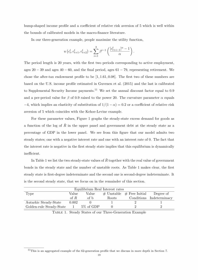
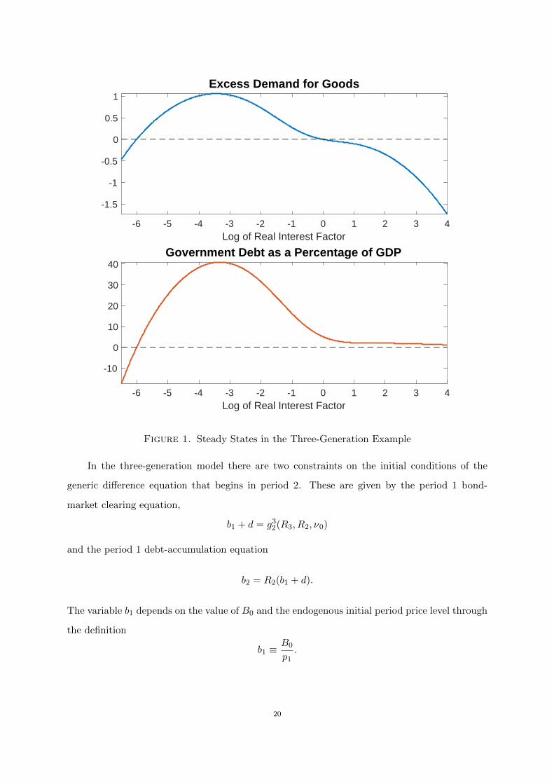
For these parameter values, Figure 1 graphs the steady-state excess demand for goods as
a function of the log of R in the upper panel and government debt at the steady state as a
percentage of GDP in the lower panel. We see from this figure that our model admits two
steady states; one with a negative interest rate and one with an interest rate of 0. The fact that
the interest rate is negative in the first steady state implies that this equilibrium is dynamically
inefficient.
In Table 1 we list the two steady-state values of R together with the real value of government
bonds in the steady state and the number of unstable roots. As Table 1 makes clear, the first
steady state is first-degree indeterminate and the second one is second-degree indeterminate. It
is the second steady state, that we focus on in the remainder of this section.
Equilibrium Real Interest ratesType Value Value # Unstable # Free Initial Degree of
of R of b Roots Conditions IndeterminacyAutarkic Steady-State 0.002 0 1 2 1Golden-rule Steady-State 1 5% of GDP 0 2 2
Table 1. Steady States of our Three-Generation Example
11This is an aggregated example of the 62-generation profile that we discuss in more depth in Section 7.
19
-6 -5 -4 -3 -2 -1 0 1 2 3 4Log of Real Interest Factor
-1.5
-1
-0.5
0
0.5
1Excess Demand for Goods
-6 -5 -4 -3 -2 -1 0 1 2 3 4Log of Real Interest Factor
-10
0
10
20
30
40Government Debt as a Percentage of GDP
Figure 1. Steady States in the Three-Generation Example
In the three-generation model there are two constraints on the initial conditions of the
generic difference equation that begins in period 2. These are given by the period 1 bond-
market clearing equation,
b1 + d = g32(R3, R2, ν0)
and the period 1 debt-accumulation equation
b2 = R2(b1 + d).
The variable b1 depends on the value of B0 and the endogenous initial period price level through
the definition
b1 ≡B0
p1.
20

These equations place two restrictions on the vector
Z0 ≡ [R3, R2, b2, b1] ≡ [XT−2, YT−2] ≡ [X1, Y1],
leaving two of the variables R3, R2, b2 and b1 to be freely chosen. In representative agent
models, the matrix J in the difference equation
Xt = JXt−1,
would have two unstable roots thus providing an additional two initial conditions to completely
determine Z0. In our calibrated example, there are no additional restrictions of this kind since
all of the roots of J are inside the unit circle when evaluated at the steady state R = 1.
Because the monetary steady state of our model displays two degrees of indeterminacy, unlike
its Ricardian counterpart, we cannot appeal to the debt valuation equation to pin down the
initial value of the price level.
6.2. Graphical illustration of the results. In this subsection, we illustrate the properties
of the model by plotting graphs of the paths of debt and real interest rates for two different
initial conditions.
In our first initial condition, we highlight the persistence of the initial period wealth dis-
tribution. We pick the initial real interest rate R2 to equal the steady state value R and we
pick the price level so that the initial real value of debt, b1, is equal to its steady state value b.
Instead of starting off the model in the steady state, we display the paths of the real interest
factor and government debt for a world where the initial middle-aged begin life with wealth that
is 3% greater than their counterpart middle-aged cohort in the steady state. Since b0 is held
constant at its steady-state value this implies that the initial old must start out with wealth
that is 3% less than their counterpart old cohort in the steady state. Specifically, we chose
ν0 ≡ R · s01(R, R, b)× 1.03.
In Figure 2 we illustrate the time paths of the real interest rate and real government debt
for this initial condition. Even though we initialize the model by setting b1 and R2 to their
steady-state values, the deviations in initial asset holdings of the middle-aged, at the expense
of the initial old, have large persistent implications for the path of market-clearing real interest
rates, and for the path of government debt. The figure shows that an initial deviation of the
initial wealth of just 3% from its steady state value causes the real interest rate to fluctuate by
21

20 40 60 80 100 120 140 160 180 200Years
0.99
1
1.01
1.02The Real Interest Factor
20 40 60 80 100 120 140 160 180 200Years
99
100
101
102
Government Debt as a Percentage of GDP
Figure 2. The impact of the initial period debt of the middle-aged exceedingits steady state by 3%
3% twenty years later and still has notable effects after 80 years. Our three-generation model
is capable of generating a very high degree of endogenous persistence in the real interest rate.
For our second experiment we feature the implications of indeterminacy for the failure of
the FTPL. The paths that we plot in the top and bottom panels of Figure 3 correspond to a
deviation in the wealth distribution caused by a 3% deviation in the initial price level. This is
similar to a wealth shock caused by a change in ν0; but instead of holding b0 fixed we allow a
change in the price level to alter the entire vector of initial wealth positions. Importantly, the
equilibrium paths of real interest rates and government debt illustrated in Figure 3 are bounded
and both variables converge back to their steady state values. The boundedness of real debt for
alternative nominal initial conditions implies that we cannot appeal to the FTPL to determine
the initial price level even when fiscal policy is active.
22

20 40 60 80 100 120 140 160 180 200Years
0.99
1
1.01
1.02
The Real Interest Factor
20 40 60 80 100 120 140 160 180 200Years
97
98
99
100
101
102
Government Debt as a Percentage of GDP
Figure 3. The impact of a 3% increase in the initial price level keeping R2 constant
If examples like this are pathological then perhaps they should be dismissed. Perhaps, for
example, risk aversion or intertemporal smoothing parameters taken from quarterly models may
not adequately describe behaviour when the horizon is 20 years? To address these criticisms,
in Section 7 we show that a 62-generation OLG model displays similar features to the three-
generation model illustrated here. Our results suggest that models with indeterminate equilibria
should be taken seriously as potential descriptions of real world phenomena.
7. A Sixty-Two Generation Example
In this section we construct a 62-generation model where each cohort begins its economic
life at age 18 and in which a period corresponds to one year. The representative person receives
an income profile when working that we calibrate to U.S. micro data and an income profile
when retired that we calibrate to U.S. Supplemental Security Income.
23

In our 62-generation example, people maximize the utility function,
u(ctt, . . . , c
tt+61
)=
62∑i=1
βi−1(
[ctt+i−1]α − 1
α
).
Explicit formulas for the excess demand functions and the savings functions for this functional
form and MATLAB code to solve the model are available in an online Technical Appendix.
We graph our calibrated income profile in Figure 4. Our representative cohort enters the
labor force at age 18, retires at age 66, and lives to age 79. We chose the lifespan to correspond
to current U.S. life expectancy at birth and we chose the retirement age to correspond to the age
at which a U.S. adult becomes eligible for social security benefits. For the working-age portion
of this profile we use data from Guvenen et al. (2015) which is available for ages 25 to 60. The
working-age income profiles for ages 18 to 24 and for ages 61 to 66, were extrapolated to earlier
and later years using log-linear interpolation. For the retirement portion we used data from the
U.S. Social Security Administration.
20 30 40 50 60 70Age
0
0.5
1
1.5
2
2.5
3
3.5
4
4.5
5
End
owm
ent
Endowment Profile
Figure 4. Normalized endowment profile. U.S. data in solid red: interpolateddata in dashed blue.
U.S. retirement income comes from three sources; private pensions, government social se-
curity benefits, and Supplemental Security Income. We treat private pensions and government24

social security benefits as perfect substitutes for private savings since the amount received in
retirement is a function of the amount contributed while working. To calibrate the available re-
tirement income that is independent of contributions, we used Supplementary Security Income
which, for the U.S., we estimate at 0.137% of GDP.12
For the remaining parameters of our model we chose an annual discount rate of 0.953 and
an elasticity of substitution of 0.17. This corresponds to α = −5 and a corresponding measure
of Arrow-Pratt risk aversion of 6. For the calibrated income profile depicted in Figure 4 and
for this choice of parameters, our model exhibits four steady state equilbria. In Section 8 we
explore the robustness of the properties of our model to alternative choices for the discount
parameter and for the risk aversion parameter.
In Figure 5 we graph the steady-state equilibria of our model. The upper panel of this
figure plots the logarithm of the gross real interest rate on the horizontal axis and the steady-
state excess demand for goods on the vertical axis. The lower panel plots government debt as
a percentage of GDP at the steady state. We see from the upper panel that the excess demand
function crosses the horizontal axis four times. And we see from the lower panel that three
of these crossings are associated with steady-state equilibria in which steady-state government
debt is equal to zero.
The three equilibria in which steady-state debt equals zero are examples of what Gale (1973)
refers to as autarkic steady-state equilibria: in these equilibria there is no possibility of trade
with future, unborn generations. The fourth steady-state is what Gale refers to as the golden-
rule equilibrium. This equilibrium always exists in OLG models and in models with population
growth it has the property that the real interest rate equals the rate of population growth. But
although the golden-rule equilibrium always exists, it is not true that the golden-rule value of
b is always non-negative.
For our model to provide a realistic theory of the value of money, it must be true that the
golden-rule steady state is associated with a positive value of b. To check that this property
does indeed hold, the reader is invited to compare the upper and lower panels of Figure 5.
The lower panel of this figure depicts the value of steady-state government debt. By inspecting
this panel it is apparent that the golden-rule steady state, which occurs when the logarithm of
12From Table 2 of the March 2018 Social Security Administration Monthly Statistical Snapshot we learn thatthe average monthly Supplemental Security Income for recipients aged 65 or older equalled $447 (with 2,240,000claimants), which implies that total monthly nominal expenditure on Supplemental Security Income equalled$1,003 million. This compares to seasonally adjusted wage and salary disbursements (A576RC1 from FRED) inFebruary 2018 of $8,618,700 million per annum, or $718,225 million per month. Back of the envelope calculationssuggest that Supplemental Security Income in retirement equalled 0.137% of total labor income.
25

-0.6 -0.5 -0.4 -0.3 -0.2 -0.1 0 0.1Log of Real Interest Factor
-50
0
50
100
Excess Demand for Goods
-0.6 -0.5 -0.4 -0.3 -0.2 -0.1 0 0.1Log of Real Interest Factor
-100
0
100
200
300
Government Debt as a Percentage of GDP
Figure 5. Steady States in the 62-Generation Model
the real interest factor equals zero, is indeed associated with positive valued government debt.
Since debt is denominated in dollars, that fact implies that money has positive value in the
golden-rule steady-state.
An equilibrium in which the interest rate is greater than or equal to the growth rate is said
to be dynamically efficient. A steady-state equilibrium in which the interest rate is less than the
growth rate is said to be dynamically inefficient. In the representative agent model, dynamically
inefficient equilbria cannot exist because they imply that the wealth of the representative agent
is unbounded. But in the OLG model, dynamically inefficient equilibria are common and, in
many examples of OLG models, dynamic inefficiency is associated with indeterminacy. In our
62-generation model however, there exist indeterminate equilibria that are dynamically efficient.
26

The values and properties of all four steady-state equilibria are reported in Table 2. We
refer to the autarkic steady states as Steady-State A, Steady-State C and Steady-State D and
to the golden-rule equilibrium as Steady-State B. We see from this table that steady states
B, C and D are associated with a non-negative interest rate and are therefore dynamically
efficient. Steady-State A is associated with a negative interest rate and is therefore dynamically
inefficient.
Equilibrium Discount FactorsType Value Value # Unstable # Free Initial Degree of
of Real Rate of b Roots Conditions IndeterminacySteady-State A -52.5% 0 60 61 1Steady-State B 0% 53.7% of GDP 59 61 2Steady-State C 2.2% 0 60 61 1Steady-State D 13.3% 0 61 61 0
Table 2. Steady States of the 62-generation Model
The 62-generation model with a calibrated income profile is similar in many respects to the
more stylized 3-generation model. In both examples, the golden-rule steady-state equilibrium
displays second degree indeterminacy. And in both examples, the steady-state price level is
positive and the initial price level is indeterminate even when fiscal policy is active. Importantly,
because the monetary steady-state is second-degree indeterminate, indeterminacy of the price
level holds even when both monetary and fiscal policy are active.
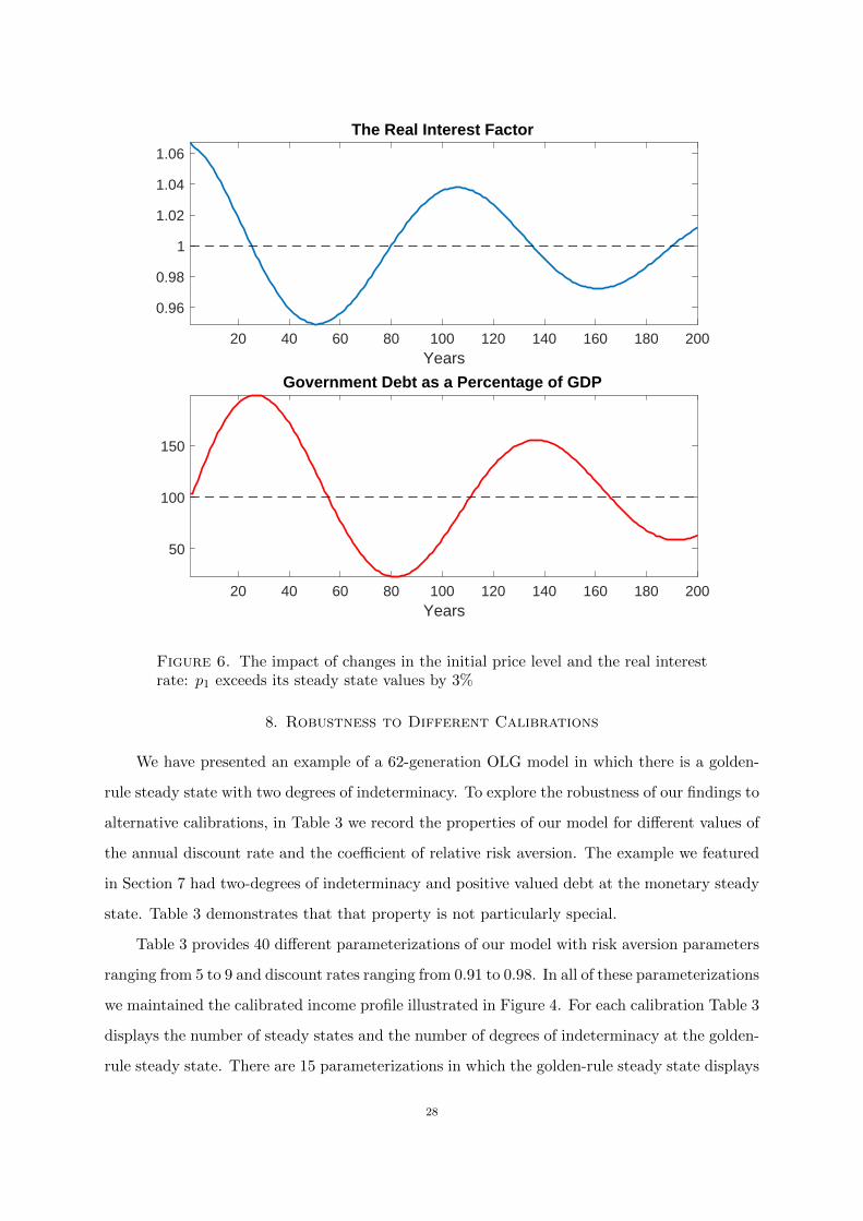
In Figure 6 we show the result of an experiment in which we perturb the initial value of b1
by 3% and we perturb the real value of the initial wealth of all of the non-generic generations by
the same amount. We restrict R2 to equal its steady state value but all other elements of Z0 are
allowed to respond to the shock to keep the path of interest rates and debt on a convergent path
back to the steady state. We refer to this shock as a 3% shock to the initial price level. Figure 6
demonstrates that the 62-generation model preserves the feature from the 3-generation example
that the return to the steady state from an arbitrary initial condition is extremely slow.
We also see from Figure 6 that our model can explain persistent periods of negative real
interest rates. The upper panel of this figure plots the path by which the real interest rate
returns to its steady state value and the lower panel plots the return path of the real value
of government debt expressed as a percentage of GDP. The figure demonstrates that small
deviations of initial conditions from their steady state values may take very long to play out
and, during the adjustment to the steady state, the real interest rate may be negative for periods
well in excess of ten years.
27
20 40 60 80 100 120 140 160 180 200Years
0.96
0.98
1
1.02
1.04
1.06
The Real Interest Factor
20 40 60 80 100 120 140 160 180 200Years
50
100
150
Government Debt as a Percentage of GDP
Figure 6. The impact of changes in the initial price level and the real interestrate: p1 exceeds its steady state values by 3%
8. Robustness to Different Calibrations
We have presented an example of a 62-generation OLG model in which there is a golden-
rule steady state with two degrees of indeterminacy. To explore the robustness of our findings to
alternative calibrations, in Table 3 we record the properties of our model for different values of
the annual discount rate and the coefficient of relative risk aversion. The example we featured
in Section 7 had two-degrees of indeterminacy and positive valued debt at the monetary steady
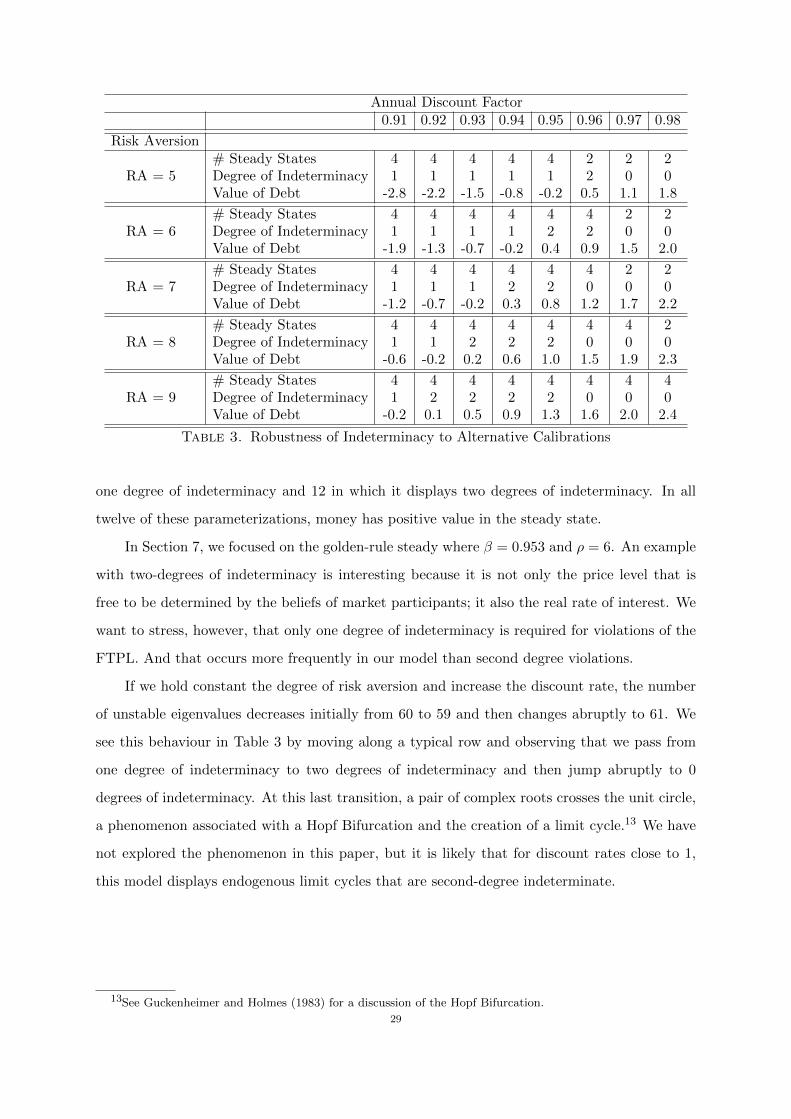
state. Table 3 demonstrates that that property is not particularly special.
Table 3 provides 40 different parameterizations of our model with risk aversion parameters
ranging from 5 to 9 and discount rates ranging from 0.91 to 0.98. In all of these parameterizations
we maintained the calibrated income profile illustrated in Figure 4. For each calibration Table 3
displays the number of steady states and the number of degrees of indeterminacy at the golden-
rule steady state. There are 15 parameterizations in which the golden-rule steady state displays
28
Annual Discount Factor0.91 0.92 0.93 0.94 0.95 0.96 0.97 0.98
Risk Aversion
RA = 5# Steady States 4 4 4 4 4 2 2 2Degree of Indeterminacy 1 1 1 1 1 2 0 0Value of Debt -2.8 -2.2 -1.5 -0.8 -0.2 0.5 1.1 1.8
RA = 6# Steady States 4 4 4 4 4 4 2 2Degree of Indeterminacy 1 1 1 1 2 2 0 0Value of Debt -1.9 -1.3 -0.7 -0.2 0.4 0.9 1.5 2.0
RA = 7# Steady States 4 4 4 4 4 4 2 2Degree of Indeterminacy 1 1 1 2 2 0 0 0Value of Debt -1.2 -0.7 -0.2 0.3 0.8 1.2 1.7 2.2
RA = 8# Steady States 4 4 4 4 4 4 4 2Degree of Indeterminacy 1 1 2 2 2 0 0 0Value of Debt -0.6 -0.2 0.2 0.6 1.0 1.5 1.9 2.3
RA = 9# Steady States 4 4 4 4 4 4 4 4Degree of Indeterminacy 1 2 2 2 2 0 0 0Value of Debt -0.2 0.1 0.5 0.9 1.3 1.6 2.0 2.4
Table 3. Robustness of Indeterminacy to Alternative Calibrations
one degree of indeterminacy and 12 in which it displays two degrees of indeterminacy. In all
twelve of these parameterizations, money has positive value in the steady state.
In Section 7, we focused on the golden-rule steady where β = 0.953 and ρ = 6. An example
with two-degrees of indeterminacy is interesting because it is not only the price level that is
free to be determined by the beliefs of market participants; it also the real rate of interest. We
want to stress, however, that only one degree of indeterminacy is required for violations of the
FTPL. And that occurs more frequently in our model than second degree violations.
If we hold constant the degree of risk aversion and increase the discount rate, the number
of unstable eigenvalues decreases initially from 60 to 59 and then changes abruptly to 61. We
see this behaviour in Table 3 by moving along a typical row and observing that we pass from
one degree of indeterminacy to two degrees of indeterminacy and then jump abruptly to 0
degrees of indeterminacy. At this last transition, a pair of complex roots crosses the unit circle,
a phenomenon associated with a Hopf Bifurcation and the creation of a limit cycle.13 We have
not explored the phenomenon in this paper, but it is likely that for discount rates close to 1,
this model displays endogenous limit cycles that are second-degree indeterminate.
13See Guckenheimer and Holmes (1983) for a discussion of the Hopf Bifurcation.
29

9. Fiscal and Monetary Policy
In the OLG models that we described in Sections 6 and 7, we assumed that fiscal policy
is active and monetary policy is passive. The assumption of an active fiscal policy follows from
our formulation of a debt accumulation equation in which there is an outstanding stock of debt
but no attempt to adjust spending or taxes to ensure that debt is repaid. The assumption
of a passive monetary policy follows from our assumption that nominal treasury liabilities are
willingly held, but that these liabilities pay a zero money interest rate. In this section we discuss
what would happen if we were to relax either of these assumptions.
9.1. Passive Fiscal policy. Consider first what would happen to our model if we were to
assume that fiscal policy is passive. Suppose, for example, that the treasury raises taxes τ t in
proportion to the real value of outstanding debt,
τ t = δbt,
where δ ≥ 0 is a debt repayment parameter. Combining this assumption with the definition of
the government debt accumulation equation leads to the amended debt accumulation equation
bt+1 = [Rt+1 − δ]bt. (13)
For values of [R − δ] < 1 the effect of this switch to a passive from an active fiscal policy is to
introduce an additional stability mechanism that increases the degree of indeterminacy at each
of the four steady states for which δ is large enough. A passive fiscal policy makes indeterminacy
more likely.
9.2. Active Monetary Policy. We model an active Taylor Rule with the equation, (Taylor,
1999),
1 + it = R
(Πt
Π
)ηΠt. (14)
Here, Π is the inflation target, and R is the steady state real interest rate. An active Taylor
rule is represented by η > 0 and a passive rule by η < 0. This rule also encompasses the special
case of an interest-rate peg for which η = −1.
In the T -generation OLG model, we have shown that the equilibrium real interest rate
is independent of the path of the inflation rate. It is fully characterized by the bond market
clearing equations
bt + dt = f(Rt+T−1, Rt+T−2, . . . , Rt−T+4, Rt−T+3),
30

and the debt accumulation equation,
bt+1 = Rt+1(bt + dt).
Conditional on a path for the real interest rate, the equilibrium inflation rate is determined
by combining the Taylor Rule, Equation (14), with the Fisher parity condition, Equation (2),
which we reproduce below,
Rt+1 ≡1 + itΠt+1
.
Combining these equations leads to the following difference equation in inflation,
Πt+1 =
(R
Rt+1
)(Πt
Π
)ηΠt, for all t ≥ 1. (15)
When monetary policy is active, Equation (15) is unstable if solved backwards for Πt+1 as
a function of Πt and Rt+1. But because the initial price level is free to be chosen, the equation
can be solved forwards to find the unique initial inflation rate, Π2, as a function of the future
path of real interest rates. Written in this way, the equation determines the unique initial value
for Π2, consistent with a bounded path for all future inflation rates. If we anchor the first period
Taylor rule by choosing p0 to be an initial condition of the model, the initial value of Π2 also
determines the initial price level, p1.
But although an active monetary policy is consistent with a unique initial price level, even
when fiscal policy is also active, it does not uniquely determine the path of real interest rates.
We have provided two examples of models, each of which display two degrees of indeterminacy
in the neighbourhood of the golden-rule steady state. That fact implies that conditional on a
given value of p1, and therefore an initial value of b1, the model still admits multiple equilibrium
paths for the real rate of interest, all of which converge back to the golden-rule steady state.
These different real rate paths are associated with different inflation paths. Real indeterminacy
implies nominal indeterminacy.
10. Conclusions
We have demonstrated an important difference between an infinitely lived representative
agent model and its overlapping generations counterpart. In the RA model, government debt
is both an asset and a liability of the representative agent. Because these two aspects exactly
offset each other, the representative agent is indifferent about the quantity of debt she holds and
31
in the simplest case the real interest rate in the corresponding model reflects time preferences
and the evolution of the endowment.
In the OLG model, the situation is different. Because the stock of government debt is
unlikely to be fully paid off during the lifetime of any generation, the assets and liabilities of the
treasury do not cancel each other out as they would in the representative agent model. As a
consequence, changes in real interest rates are redistributive across cohorts, and they may lead
to fluctuations in the demand for government bonds that are self-stabilizing.
In our calibrated model the golden-rule steady state equilibrium is both dynamically effi-
cient and second-degree indeterminate. As long as the primary deficit or the primary surplus
is not too large, the fiscal authority can conduct policies that are unresponsive to endogenous
changes in the level of its outstanding debt. Monetary and fiscal policy can both be active at
the same time.
Our findings challenge established views about what constitutes a good combination of fiscal
and monetary policies. Our agents are rational and have rational expectations. Nevertheless,
the price level and the real interest rate are not uniquely determined by what most economists
would recognize as economic fundamentals, even when the central bank and the treasury both
pursue active policies. These features of our model lead to very different conclusions from those
of the RA approach.
If the FTPL holds, a benevolent monetary policy maker who pursues an interest rate peg
might rely on fiscal policy to anchor the price level. In the OLG model we studied here that is
no longer possible. Giving up on active monetary policy implies that the policy maker has also
abandoned the ability of active monetary policy to provide a nominal anchor.
Our model also leads to non-standard advice to fiscal policy makers. In an RA model, the
fiscal policy maker must raise taxes or lower expenditures in response to recessions, however they
are caused. In Farmer and Zabczyk (2018) we showed, in a two-generation OLG model, that
equilibrium debt dynamics can be self-stabilizing. In this paper we have extended our previous
analysis to a calibrated 62-generation OLG model. In our 62-period calibrated example, a fiscal
policy that does not respond to endogenous fluctuations in debt, can safely be pursued, at least
for small values of the primary deficit, without the fear that a policy of this kind will lead to
an exploding debt level as a fraction of GDP.
32

References
Aiyagari, S. R. (1985): “Observational Equivalence of the Overlapping Generations and the
Discounted Dynamic Programming Frameworks for One-sector Growth,” Journal of Eco-
nomic Theory, 35, 202–221.
Auerbach, A. and L. Kotlikoff (1987): Dynamic Fiscal Policy, Cambridge: Cambridge
University Press.
Auerbach, A. J. (2003): “Fiscal Policy, Past and Present,” Brookings Papers on Economic
Activity, 34, 75–138.
Azariadis, C. (1981): “Self-fulfilling Prophecies,” Journal of Economic Theory, 25, 380–396.
Azariadis, C., J. Bullard, A. Singh, and J. Suda (2015): “Optimal Monetary Policy at
the Zero Lower Bound,” Federal Reserve Bank of St Louis WP Series, 1–47.
Barro, R. J. (1974): “Are Government Bonds Net Wealth?” Journal of Political Economy,
82, 1095–1117.
Becker Friedman Institute (2016): “Determining the Value of Money: Next Steps for the
Fiscal Theory of the Price Level,” https://www.youtube.com/watch?v=22RZx9LbFKw.
Benhabib, J., S. Schmitt-Grohe, and M. Uribe (2001): “The Perils of Taylor Rules,”
Journal of Economic Theory, 96, 40–69.
——— (2002): “Avoiding Liquidity Traps,” Journal of Political Economy, 110, 535–563.
Blanchard, O. J. (1985): “Debt, Deficits, and Finite Horizons,” Journal of Political Economy,
93, 223–247.
Blanchard, O. J. and C. M. Kahn (1980): “The Solution of Linear Difference Models
Under Rational Expectations,” Econometrica, 48, 1305–1311.
Buiter, W. H. (2002): “The Fiscal Theory of the Price Level: A Critique,” The Economic
Journal, 112, 459–480.
——— (2017): “The Fallacy of the Fiscal Theory of the Price Level Once More,” CDEP-CGEG
Working Paper Series.
Castaneda, A., J.-D. Gimenez, and J. V. Rıos-Rull (2003): “Accounting for the US
Earnings and Wealth Inequality,” Journal of Political Economy, 111, 818–857.
Cochrane, J. (2005): “Money as Stock,” Journal of Monetary Economics, 52, 501–528.
——— (2018): “Stepping on a Rake: The Fiscal Theory of Monetary Policy,” European Eco-
nomic Review, 101, 354–375.
Eggertsson, G. B., N. R. Mehrota, and J. A. Robbins (2019): “A Model of Secular
Stagnation: Theory and Quantitative Evaluation,” American Economic Journal: Macroeco-
nomics, 11, 1–48.
Farmer, R. E. A. (1986): “Deficits and Cycles,” Journal of Economic Theory, 40, 77–88.
——— (1999): The Macroeconomics of Self-Fulfilling Prophecies, Cambridge, MA: MIT Press,
second ed.
——— (2018): “Pricing Assets in a Perpetual Youth Model,” Review of Economic Dynamics,
30, 446–460.
Farmer, R. E. A., V. Khramov, and G. Nicolo (2015): “Solving and Estimating Indeter-
minate DSGE Models,” Journal of Economic Dynamics and Control., 54, 17–36.
Farmer, R. E. A. and M. Woodford (1997): “Self-fulfilling Prophecies and the Business
Cycle,” Macroeconomic Dynamics, 1, 740–769.
33
Farmer, R. E. A. and P. Zabczyk (2018): “The Household Fallacy,” Economics Letters,
169, 83–86.
Gale, D. (1973): “Pure exchange equilibrium of dynamic economic models,” Journal of Eco-
nomic Theory, 6, 12–36.
Golub, G. H. and C. F. VanLoan (1996): Matrix Computations, Baltimore, Maryland: The
Johns Hopkins University Press, third ed.
Guckenheimer, J. and P. Holmes (1983): Nonlinear Oscillations, Dynamical Systems and
Bifurcations of Vector Fields, Springer.
Guvenen, F., F. Karahan, S. Ozkan, and J. Song (2015): “What Do Data on Millions
of U.S. Workers Reveal about Life-Cycle Earnings Risk?” Working Paper 20913, National
Bureau of Economic Research.
Kehoe, T. J. and D. K. Levine (1983): “Indeterminacy of Relative Prices in Overlapping
Generations Models,” Unpublished MIT Working Paper no. 313.
——— (1985): “Comparative Statics and Perfect Foresight in Infinite Horizon Economies,”
Econometrica, 53, 433–453.
Kubler, F. and K. Schmedders (2011): “Lifecycle Portfolio Choice, the Wealth Distribution
and Asset Prices,” University of Zurich, mimeo.
Leeper, E. M. (1991): “Equilibria Under ‘Active’ and ‘Passive’ Monetary and Fiscal Policies,”
Journal of Monetary Economics, 27, 129–147.
Martin, A. and J. Ventura (2011): “Theoretical Notes on Bubbles and the Current Crisis,”
IMF Economic Review, 59, 6–40.
——— (2012): “Economic Growth with Bubbles,” American Economic Review, 102, 3033–3058.
McCallum, B. T. (1981): “Price Level Determinacy With an Interest Rate Policy Rule and
Rational Expectations,” Journal of Monetary Economics, 8, 319–329.
——— (1999): “Issues in the Design of Monetary Policy Rules,” in Handbook of Macroeco-
nomics, Vol. 1C, ed. by J. B. Taylor and M. Woodford, Amsterdam: Elsevier Science, 1483–
1530.
——— (2001): “Indeterminacy, Bubbles, and the Fiscal Theory of Price Level Determination,”
Journal of Monetary Economics, 47, 19–30.
——— (2003): “Is the Fiscal Theory of the Price Level Learnable?” Scottish Journal of Political
Economy, 50, 634–639.
McCallum, B. T. and E. Nelson (2005): “Monetary and Fiscal Theories of the Price Level:
The Irreconcilable Differences,” Oxford Review of Economic Poicy, 21, 565–583.
Miao, J. and P. Wang (2012): “Bubbles and Total Factor Productivity,” American Economic
Review: Papers and Proceedings, 102, 82–87.
Miao, J., P. Wang, and Z. Xu (2012): “Stock Market Bubbles and Unemployment,” Boston
University mimeo.
O’Driscoll, G. P. J. (1977): “The Ricardian Nonequivalence Theorem,” Journal of Political
Economy, 85, 207–210.
Poterba, J. M. and L. H. Summers (1987): “Finite lifetimes and the effects of budget
deficits on national saving,” Journal of Monetary Economics, 20, 369 – 391.
Reichlin, P. (1992): “Endogenous Cycles with Long-Lived Agents,” Journal of Economic
Dynamics and Control, 16, 243–266.
34

Ricardo, D. (1888): “Essay on the Funding System,” in The Works of David Ricardo. With
a Notice of the Life and Writings of the Author., ed. by J. R. McCulloch, John Murray.
Rıos-Rull, J. V. and V. Quadrini (1997): “Understanding the US Distribution of Wealth,”
Federal Reserve Bank of Minneapolis Quarterly Review, 21, 22–36.
Rıos-Rull, V. (1996): “Life-Cycle Economies and Aggregate Fluctuations,” Review of Eco-
nomic Studies, 63, 465–489.
Samuelson, P. A. (1958): “An Exact Consumption-Loan Model of Interest With or Without
the Social Contrivance of Money,” Journal of Political Economy, 66, 467–482.
Sargent, T. J. and N. Wallace (1975): “’Rational’ Expectations, the Optimal Monetary
Instrument, and the Optimal Money Supply Rule,” Journal of Political Economy, 83, 241–
254.
Sims, C. A. (1994): “A Simple Model for Study of the Determination of the Price Level and
the Interaction of Monetary and Fiscal Policy,” Economic Theory, 4, 381–399.
——— (2001): “Solving Linear Rational Expectations Models,” Journal of Computational Eco-
nomics, 20, 1–20.
Summers, L., C. Carroll, and A. S. Blinder (1987): “Why is U.S. National Saving so
Low?” Brookings Papers on Economic Activity, 1987, 607–642.
Taylor, J. B. (1999): “An Historical Analysis of Monetary Policy Rules,” in Monetary Policy
Rules, ed. by J. B. Taylor, Chicago: University of Chicago Press, 319–341.
Tirole, J. (1985): “Asset Bubbles and Overlapping Generations,” Econometrica, 53, 1499–
1528.
Woodford, M. (1994): “Monetary Policy and Price Level Determinacy in a Cash-in-Advance
Economy,” Economic Theory, 4, 345–380.
——— (1995): “Price-Level Determinacy without Control of a Monetary Aggegrate,” Carnegie-
Rochester Conference Series on Public Policy, 43, 1–46.
——— (2001): “Fiscal Requirements for Price Stability,” Journal of Money, Credit, and Bank-
ing, 33, 669–728.
35