Embed Size (px)
Citation preview

K12048_cover.fhmx 7/25/11 3:11 PM Page 1
C M Y CM MY CY CMY K
ELLIS H. DILL
The Finite ElementMethod for Mechanicsof Solids withANSYS Applications
The Finite Element Method for Mechanicsof Solids with ANSYS Applications
K12048
6000 Broken Sound Parkway, NWSuite 300, Boca Raton, FL 33487711 Third AvenueNew York, NY 100172 Park Square, Milton ParkAbingdon, Oxon OX14 4RN, UK
an informa business
The Finite Element Method for Mechanicsof Solids with ANSYS Applications
DILL
While the finite element method (FEM) has become the standard technique used to solvestatic and dynamic problems associated with structures and machines, ANSYS softwarehas developed into the engineer’s software of choice to model and numerically solvethose problems.An invaluable tool to help engineers master and optimize analysis, The Finite ElementMethod for Mechanics of Solids with ANSYS Applications explains the foundations of FEMin detail, enabling engineers to use it properly to analyze stress and interpret the outputof a finite element computer program such as ANSYS.Illustrating presented theory with a wealth of practical examples, this book covers topicsincluding
• Essential background on solid mechanics (including small- and large-deformationelasticity, plasticity, viscoelasticity) and mathematics
• Advanced finite element theory and associated fundamentals, with examples• Use of ANSYS to derive solutions for problems that deal with vibration, wave
propagation, fracture mechanics, plates and shells, and contact
Totally self-contained, this text presents step-by-step instructions on how to use ANSYSParametric Design Language (APDL) and the ANSYS Workbench to solve problemsinvolving static/dynamic structural analysis (both linear and nonlinear) and heat transfer,among other areas. It will quickly become a welcome addition to any engineering library,equally useful to students and experienced engineers.
Mechanical Engineering
ELLIS H. DILL
The Finite ElementMethod for Mechanicsof Solids withANSYS Applications
Advances in EngineeringAÊSeriesÊofÊReferenceÊBooks,ÊMonographs,ÊandÊTextbooks
Series Editor
Haym BenaroyaDepartment of Mechanical and Aerospace Engineering
Rutgers University
Published Titles:
The Finite Element Method for Mechanics of Solids with ANSYS Applications, Ellis H. Dill
Dynamics of Tethered Space Systems, A. P. Alpatov, V. V. Beletsky, V. I. Dranovskii, V. S. Khoroshilov, A. V. Pirozhenko, H. Troger, and A. E. Zakrzhevskii
Lunar Settlements, Haym Benaroya
Handbook of Space Engineering, Archaeology and Heritage, Ann Darrin and Beth O’Leary
Spatial Variation of Seismic Ground Motions: Modeling and Engineering Applications, Aspasia Zerva
Fundamentals of Rail Vehicle Dynamics: Guidance and Stability, A. H. Wickens
Advances in Nonlinear Dynamics in China: Theory and Applications, Wenhu Huang
Virtual Testing of Mechanical Systems: Theories and Techniques, Ole Ivar Sivertsen
Nonlinear Random Vibration: Analytical Techniques and Applications, Cho W. S. To
Handbook of Vehicle-Road Interaction, David Cebon
Nonlinear Dynamics of Compliant Offshore Structures, Patrick Bar-Avi and Haym Benaroya

The Finite ElementMethod for Mechanicsof Solids withANSYS Applications
ELLIS H. DILL
CRC Press is an imprint of theTaylor & Francis Group, an informa business
Boca Raton London New York

CRC PressTaylor & Francis Group6000 Broken Sound Parkway NW, Suite 300Boca Raton, FL 33487-2742
© 2011 by Taylor & Francis Group, LLCCRC Press is an imprint of Taylor & Francis Group, an Informa business
No claim to original U.S. Government worksVersion Date: 20140602
International Standard Book Number-13: 978-1-4398-4584-4 (eBook - PDF)
This book contains information obtained from authentic and highly regarded sources. Reasonable efforts have been made to publish reliable data and information, but the author and publisher cannot assume responsibility for the validity of all materials or the consequences of their use. The authors and publishers have attempted to trace the copyright holders of all material reproduced in this publication and apologize to copyright holders if permission to publish in this form has not been obtained. If any copyright material has not been acknowledged please write and let us know so we may rectify in any future reprint.
Except as permitted under U.S. Copyright Law, no part of this book may be reprinted, reproduced, transmit-ted, or utilized in any form by any electronic, mechanical, or other means, now known or hereafter invented, including photocopying, microfilming, and recording, or in any information storage or retrieval system, without written permission from the publishers.
For permission to photocopy or use material electronically from this work, please access www.copyright.com (http://www.copyright.com/) or contact the Copyright Clearance Center, Inc. (CCC), 222 Rosewood Drive, Danvers, MA 01923, 978-750-8400. CCC is a not-for-profit organization that provides licenses and registration for a variety of users. For organizations that have been granted a photocopy license by the CCC, a separate system of payment has been arranged.
Trademark Notice: Product or corporate names may be trademarks or registered trademarks, and are used only for identification and explanation without intent to infringe.
Visit the Taylor & Francis Web site athttp://www.taylorandfrancis.com
and the CRC Press Web site athttp://www.crcpress.com

v
ContentsPreface.................................................................................................................... xiiiAuthor ......................................................................................................................xv
1Chapter Finite Element Concepts ......................................................................1
1.1 Introduction ...............................................................................11.2 Direct Stiffness Method ............................................................2
1.2.1 Merging the Element Stiffness Matrices ......................31.2.2 Augmenting the Element Stiffness Matrix ..................51.2.3 Stiffness Matrix Is Banded ..........................................5
1.3 The Energy Method ...................................................................51.4 Truss Example ...........................................................................71.5 Axially Loaded Rod Example ................................................. 13
1.5.1 Augmented Matrices for the Rod ............................... 161.5.2 Merge of Element Matrices for the Rod ..................... 17
1.6 Force Method ........................................................................... 181.7 Other Structural Components .................................................. 21
1.7.1 Space Truss ................................................................. 211.7.2 Beams and Frames ..................................................... 21
1.7.2.1 General Beam Equations ............................241.7.3 Plates and Shells .........................................................261.7.4 Two- or Three-Dimensional Solids ............................26
1.8 Problems ..................................................................................26References ..........................................................................................28Bibliography .......................................................................................28
2Chapter Linear Elasticity .................................................................................29
2.1 Basic Equations .......................................................................292.1.1 Geometry of Deformation ..........................................292.1.2 Balance of Momentum ...............................................302.1.3 Virtual Work ..............................................................302.1.4 Constitutive Relations ................................................. 312.1.5 Boundary Conditions and Initial Conditions ............ 332.1.6 Incompressible Materials ........................................... 332.1.7 Plane Strain ................................................................342.1.8 Plane Stress ................................................................342.1.9 Tensile Test ................................................................. 352.1.10 Pure Shear ..................................................................362.1.11 Pure Bending ..............................................................362.1.12 Bending and Shearing ................................................ 37

vi Contents
2.1.13 Properties of Solutions ............................................... 382.1.14 A Plane Stress Example with a Singularity in
Stress ..........................................................................402.2 Potential Energy ...................................................................... 42
2.2.1 Proof of Minimum Potential Energy ..........................442.3 Matrix Notation ....................................................................... 452.4 Axially Symmetric Deformations ...........................................48
2.4.1 Cylindrical Coordinates .............................................482.4.2 Axial Symmetry ......................................................... 492.4.3 Plane Stress and Plane Strain .....................................50
2.5 Problems ..................................................................................50References .......................................................................................... 51Bibliography ....................................................................................... 52
3Chapter Finite Element Method for Linear Elasticity ..................................... 53
3.1 Finite Element Approximation ................................................543.1.1 Potential Energy ......................................................... 553.1.2 Finite Element Equations ........................................... 573.1.3 Basic Equations in Matrix Notation ........................... 583.1.4 Basic Equations Using Virtual Work ......................... 593.1.5 Underestimate of Displacements ................................603.1.6 Nondimensional Equations ........................................ 613.1.7 Uniaxial Stress ........................................................... 63
3.2 General Equations for an Assembly of Elements ....................663.2.1 Generalized Variational Principle ..............................683.2.2 Potential Energy .........................................................693.2.3 Hybrid Displacement Functional ................................693.2.4 Hybrid Stress and Complementary Energy ................ 703.2.5 Mixed Methods of Analysis ....................................... 72
3.3 Nearly Incompressible Materials ............................................. 753.3.1 Nearly Incompressible Plane Strain ........................... 78
Bibliography ....................................................................................... 79
4Chapter The Triangle and the Tetrahedron ...................................................... 81
4.1 Linear Functions over a Triangular Region ............................. 814.2 Triangular Element for Plane Stress and Plane Strain ............844.3 Plane Quadrilateral from Four Triangles ................................88
4.3.1 Square Element Formed from Four Triangles ..........904.4 Plane Stress Example: Short Beam .........................................93
4.4.1 Extrapolation of the Solution ......................................964.5 Linear Strain Triangles ............................................................974.6 Four-Node Tetrahedron ...........................................................984.7 Ten-Node Tetrahedron .............................................................994.8 Problems ..................................................................................99
Contents vii
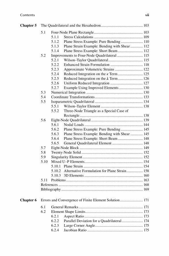
5Chapter The Quadrilateral and the Hexahedron ............................................ 103
5.1 Four-Node Plane Rectangle ................................................... 1035.1.1 Stress Calculations ................................................... 1095.1.2 Plane Stress Example: Pure Bending ....................... 1105.1.3 Plane Strain Example: Bending with Shear ............. 1125.1.4 Plane Stress Example: Short Beam .......................... 112
5.2 Improvements to Four-Node Quadrilateral ........................... 1155.2.1 Wilson–Taylor Quadrilateral .................................... 1155.2.2 Enhanced Strain Formulation .................................. 1185.2.3 Approximate Volumetric Strains ............................. 1225.2.4 Reduced Integration on the κ Term .......................... 1255.2.5 Reduced Integration on the λ Term .......................... 1265.2.6 Uniform Reduced Integration .................................. 1275.2.7 Example Using Improved Elements ......................... 130
5.3 Numerical Integration ........................................................... 1305.4 Coordinate Transformations .................................................. 1335.5 Isoparametric Quadrilateral .................................................. 134
5.5.1 Wilson–Taylor Element ............................................ 1385.5.2 Three-Node Triangle as a Special Case of
Rectangle .................................................................. 1385.6 Eight-Node Quadrilateral ...................................................... 139
5.6.1 Nodal Loads ............................................................. 1445.6.2 Plane Stress Example: Pure Bending ....................... 1455.6.3 Plane Stress Example: Bending with Shear ............. 1455.6.4 Plane Stress Example: Short Beam .......................... 1485.6.5 General Quadrilateral Element ................................ 148
5.7 Eight-Node Block .................................................................. 1495.8 Twenty-Node Solid ................................................................ 1525.9 Singularity Element ............................................................... 1525.10 Mixed U–P Elements............................................................. 154
5.10.1 Plane Strain .............................................................. 1545.10.2 Alternative Formulation for Plane Strain ................. 1585.10.3 3D Elements ............................................................. 160
5.11 Problems ................................................................................ 163References ........................................................................................ 168Bibliography ..................................................................................... 169
6Chapter Errors and Convergence of Finite Element Solution ........................ 171
6.1 General Remarks ................................................................... 1716.2 Element Shape Limits ............................................................ 173
6.2.1 Aspect Ratio ............................................................. 1736.2.2 Parallel Deviation for a Quadrilateral ...................... 1746.2.3 Large Corner Angle.................................................. 1756.2.4 Jacobian Ratio .......................................................... 175

viii Contents
6.3 Patch Test ............................................................................... 1766.3.1 Wilson–Taylor Quadrilateral .................................... 178
References ........................................................................................ 180
7Chapter Heat Conduction in Elastic Solids .................................................... 181
7.1 Differential Equations and Virtual Work .............................. 1817.2 Example Problem: One-Dimensional Transient Heat Flux ... 1857.3 Example: Hollow Cylinder .................................................... 1877.4 Problems ................................................................................ 188
8Chapter Finite Element Method for Plasticity ............................................... 191
8.1 Theory of Plasticity ............................................................... 1918.1.1 Tensile Test ............................................................... 1948.1.2 Plane Stress .............................................................. 1958.1.3 Summary of Plasticity .............................................. 196
8.2 Finite Element Formulation for Plasticity ............................. 1978.2.1 Fundamental Solution .............................................. 1988.2.2 Iteration to Improve the Solution .............................. 199
8.3 Example: Short Beam ............................................................ 2018.4 Problems ................................................................................203Bibliography .....................................................................................204
9Chapter Viscoelasticity ..................................................................................205
9.1 Theory of Linear Viscoelasticity ...........................................2059.1.1 Recurrence Formula for History .............................. 2109.1.2 Viscoelastic Example ............................................... 211
9.2 Finite Element Formulation for Viscoelasticity .................... 2159.2.1 Basic Step-by-Step Solution Method ........................ 2169.2.2 Step-by-Step Calculation with Load Correction ...... 2179.2.3 Plane Strain Example ............................................... 218
9.3 Problems ................................................................................ 219Bibliography .....................................................................................220
1Chapter 0 Dynamic Analyses ........................................................................... 221
10.1 Dynamical Equations ............................................................ 22110.1.1 Lumped Mass ........................................................... 22110.1.2 Consistent Mass ....................................................... 222
10.2 Natural Frequencies ..............................................................22410.2.1 Lumped Mass ...........................................................22410.2.2 Consistent Mass .......................................................225
10.3 Mode Superposition Solution ................................................22510.4 Example: Axially Loaded Rod .............................................. 227

Contents ix
10.4.1 Exact Solution for Axially Loaded Rod ................... 22710.4.2 Finite Element Model ............................................... 229
10.4.2.1 One-Element Model .................................. 22910.4.2.2 Two-Element Model .................................230
10.4.3 Mode Superposition for Continuum Model of the Rod ..................................................................... 232
10.5 Example: Short Beam ............................................................ 23610.6 Dynamic Analysis with Damping ........................................ 237
10.6.1 Viscoelastic Damping .............................................. 23810.6.2 Viscous Body Force ................................................ 23910.6.3 Analysis of Damped Motion by Mode
Superposition ............................................................24010.7 Numerical Solution of Differential Equations ....................... 241
10.7.1 Constant Average Acceleration ................................ 24110.7.2 General Newmark Method ....................................... 24310.7.3 General Methods ......................................................244
10.7.3.1 Implicit Methods in General ....................24410.7.3.2 Explicit Methods in General ....................244
10.7.4 Stability Analysis of Newmark’s Method ................24510.7.5 Convergence, Stability, and Error ............................24610.7.6 Example: Numerical Integration for Axially
Loaded Rod .............................................................. 24710.8 Example: Analysis of Short Beam .........................................24910.9 Problems ................................................................................ 251Bibliography ..................................................................................... 253
1Chapter 1 Linear Elastic Fracture Mechanics .................................................. 255
11.1 Fracture Criterion .................................................................. 25511.1.1 Analysis of Sheet ...................................................... 25711.1.2 Fracture Modes......................................................... 258
11.1.2.1 Mode I ....................................................... 25811.1.2.2 Mode II ..................................................... 25911.1.2.3 Mode III ................................................... 259
11.2 Determination of K by Finite Element Analysis ...................26011.2.1 Crack Opening Displacement Method .....................260
11.3 J-Integral for Plane Regions .................................................. 26311.4 Problems ................................................................................ 267References ........................................................................................268Bibliography .....................................................................................268
1Chapter 2 Plates and Shells ...............................................................................269
12.1 Geometry of Deformation .....................................................26912.2 Equations of Equilibrium ...................................................... 27012.3 Constitutive Relations for an Elastic Material ....................... 271

x Contents
12.4 Virtual Work .......................................................................... 27312.5 Finite Element Relations for Bending ................................... 27612.6 Classical Plate Theory ...........................................................28012.7 Plate Bending Example ......................................................... 28212.8 Problems ................................................................................287References ........................................................................................288Bibliography ..................................................................................... 289
1Chapter 3 Large Deformations.......................................................................... 291
13.1 Theory of Large Deformations .............................................. 29113.1.1 Virtual Work ............................................................29213.1.2 Elastic Materials ....................................................... 29313.1.3 Mooney–Rivlin Model of an Incompressible
Material ....................................................................29713.1.4 Generalized Mooney–Rivlin Model ......................... 29813.1.5 Polynomial Formula ................................................. 30113.1.6 Ogden’s Function ......................................................30313.1.7 Blatz–Ko Model .......................................................30413.1.8 Logarithmic Strain Measure ....................................30613.1.9 Yeoh Model ..............................................................30713.1.10 Fitting Constitutive Relations to
Experimental Data ...................................................30813.1.10.1 Volumetric Data .....................................30813.1.10.2 Tensile Test .............................................30813.1.10.3 Biaxial Test .............................................309
13.2 Finite Elements for Large Displacements .............................30913.2.1 Lagrangian Formulation ........................................... 31113.2.2 Basic Step-by-Step Analysis .................................... 31213.2.3 Iteration Procedure ................................................... 31213.2.4 Updated Reference Configuration ............................ 31313.2.5 Example I ................................................................. 31513.2.6 Example II ................................................................ 315
13.3 Structure of Tangent Modulus ............................................... 31713.4 Stability and Buckling ........................................................... 318
13.4.1 Beam–Column ......................................................... 31913.5 Snap-Through Buckling ........................................................ 319
13.5.1 Shallow Arch ............................................................ 32313.6 Problems ................................................................................ 324References ........................................................................................ 326Bibliography ..................................................................................... 326
1Chapter 4 Constraints and Contact ................................................................... 327
14.1 Application of Constraints ..................................................... 32714.1.1 Lagrange Multipliers ................................................ 327

Contents xi
14.1.2 Perturbed Lagrangian Method ................................. 32914.1.3 Penalty Functions ..................................................... 33114.1.4 Augmented Lagrangian Method .............................. 332
14.2 Contact Problems ................................................................... 33314.2.1 Example: A Truss Contacts a Rigid Foundation ...... 333
14.2.1.1 Load Fy > 0 Is Applied with Fx = 0 ........... 33514.2.1.2 Loads Are Ramped Up Together:
Fx = 27α, Fy = 12.8α .................................. 33614.2.2 Lagrange Multiplier, No Friction Force ................... 337
14.2.2.1 Stick Condition ......................................... 33814.2.2.2 Slip Condition ........................................... 338
14.2.3 Lagrange Multiplier, with Friction ........................... 33814.2.3.1 Stick Condition ......................................... 33914.2.3.2 Slip Condition ........................................... 339
14.2.4 Penalty Method .......................................................34014.2.4.1 Stick Condition ......................................... 34114.2.4.2 Slip Condition ........................................... 341
14.3 Finite Element Analysis......................................................... 34114.3.1 Example: Contact of a Cylinder with a Rigid
Plane ......................................................................... 34214.3.2 Hertz Contact Problem ............................................. 343
14.4 Dynamic Impact ....................................................................34614.5 Problems ................................................................................ 347References ........................................................................................348Bibliography .....................................................................................348
1Chapter 5 ANSYS APDL Examples ................................................................. 349
15.1 ANSYS Instructions .............................................................. 34915.1.1 ANSYS File Names .................................................. 35115.1.2 Graphic Window Controls........................................ 352
15.1.2.1 Graphics Window Logo ............................ 35215.1.2.2 Display of Model ...................................... 35215.1.2.3 Display of Deformed and Undeformed
Shape White on White .............................. 35215.1.2.4 Adjusting Graph Colors ............................ 35215.1.2.5 Printing from Windows Version of
ANSYS ..................................................... 35315.1.2.6 Some Useful Notes ................................... 353
15.2 ANSYS Elements SURF153, SURF154 ................................ 35315.3 Truss Example ....................................................................... 35415.4 Beam Bending ....................................................................... 35715.5 Beam with a Distributed Load ..............................................36015.6 One Triangle .......................................................................... 36115.7 Plane Stress Example Using Triangles ..................................36415.8 Cantilever Beam Modeled as Plane Stress ............................366
xii Contents
15.9 Plane Stress: Pure Bending ................................................... 36915.10 Plane Strain Bending Example .............................................. 37115.11 Plane Stress Example: Short Beam ....................................... 37615.12 Sheet with a Hole ................................................................... 379
15.12.1 Solution Procedure ................................................... 37915.13 Plasticity Example ................................................................. 38115.14 Viscoelasticity Creep Test ..................................................... 38715.15 Viscoelasticity Example ........................................................ 39115.16 Mode Shapes and Frequencies of a Rod ................................ 39415.17 Mode Shapes and Frequencies of a Short Beam ................... 39715.18 Transient Analysis of Short Beam ......................................... 39815.19 Stress Intensity Factor by Crack Opening Displacement ......40015.20 Stress Intensity Factor by J-Integral ......................................40215.21 Stretching of a Nonlinear Elastic Sheet.................................40515.22 Nonlinear Elasticity: Tensile Test ..........................................40815.23 Column Buckling .................................................................. 41215.24 Column Post-Buckling .......................................................... 41515.25 Snap-Through ........................................................................ 41715.26 Plate Bending Example ......................................................... 42015.27 Clamped Plate........................................................................ 42315.28 Gravity Load on a Cylindrical Shell ..................................... 42515.29 Plate Buckling ....................................................................... 42915.30 Heated Rectangular Rod ....................................................... 43215.31 Heated Cylindrical Rod ......................................................... 43415.32 Heated Disk ........................................................................... 43815.33 Truss Contacting a Rigid Foundation ....................................44215.34 Compression of a Rubber Cylinder between Rigid Plates.....44615.35 Hertz Contact Problem .......................................................... 45115.36 Elastic Rod Impacting a Rigid Wall ...................................... 45615.37 Curve Fit for Nonlinear Elasticity Using Blatz–Ko Model ...46015.38 Curve Fit for Nonlinear Elasticity Using Polynomial Model....464Bibliography .....................................................................................469
1Chapter 6 ANSYS Workbench .......................................................................... 471
16.1 Two- and Three-Dimensional Geometry .............................. 47116.2 Stress Analysis ....................................................................... 47216.3 Short Beam Example ............................................................. 473
16.3.1 Short Beam Geometry .............................................. 47316.3.2 Short Beam, Static Loading ..................................... 47416.3.3 Short Beam, Transient Analysis ............................... 476
16.4 Filleted Bar Example ............................................................. 47716.5 Sheet with a Hole ...................................................................480Bibliography ..................................................................................... 482
Index ...................................................................................................................... 483

xiii
PrefaceThe purpose of this book is to explain application of the finite element method to problems in the mechanics of solids. It is intended for practicing engineers who use the finite element method for stress analysis and for graduate students in engi-neering who want to understand the finite element method for their research. It is also designed as a textbook for a graduate course in engineering. Application of the finite element method is illustrated by using the ANSYS computer program. Step-by-step instructions for the use of ANSYS Parametric Design Language (APDL) and ANSYS Workbench in more than 40 examples are included.
The required background material in the mechanics of solids is provided so that the work is self-contained for the knowledgeable reader. A more complete treat-ment of solid mechanics is provided in the book Continuum Mechanics: Elasticity, Plasticity, Viscoelasticity by Ellis H. Dill (CRC Press, 2007). References to that book are noted in this book on an applicable page by a footnote (Dill: specific r eferral detail).
This book is not intended as a detailed reference book on the use of the ANSYS system. However, Chapters 15 and 16 contain detailed steps for the application of ANSYS in numerous examples, which will enable the user to become fairly profi-cient in the use of this software. The new user should begin with one of the tutorials provided by ANSYS or with one of the elementary books listed in the bibliogra-phy in Chapters 15 and 16. This book was written using Version 12.1. However, the examples in Chapters 15 and 16 can be executed using either Version 12 or Version 13. I do not pretend to present a detailed analysis of finite element as implemented by ANSYS. I do not have access to their computer coding. I believe that the elements they are using are essentially the same as those presented here, although they may differ in some details.
I have attempted to cover only the essentials of the subject and to provide the tools necessary for comprehension of the technical literature and the commercial finite element programs. I apologize in advance to all of the originators of this material who are not referenced. I have long ago forgotten where I learned the theory.
BoCheng Jin helped with the preparation of the manuscript and provided many corrections to it. Of course, any remaining errors are mine alone.
ANSYS, ANSYS Workbench, and ANSYS APDL are trademarks of ANSYS, Inc. The software was used for examples, and the results cited, by special permission from ANSYS, Inc.


xv
AuthorEllis H. Dill obtained his BS, MS, and PhD from the University of California (Berkeley) in civil engineering. He taught aeronautical engineering at the University of Washington (Seattle) from 1956 to 1977. He was dean of engineering at Rutgers, the State University of New Jersey, from 1977 to 1998. Dr. Dill is currently a univer-sity professor at Rutgers, teaching mechanical and aerospace engineering. His prin-cipal research areas include aircraft structures, analysis of plates and shells, solid mechanics, and the finite element method of stress analysis. He can be reached by email at [email protected].


1
1 Finite Element Concepts
1.1 IntroductIon
The finite element method (FEM) has developed along two paths. From the math-ematical point of view, it is a method of constructing a function that makes the potential energy a minimum. From the engineering point of view, it is a method of assembling structural elements, which can be separately analyzed, into a global equation of equilibrium for the structure. The mathematical point of view makes the FEM a special form of the Rayleigh–Ritz method, which has a long history. The modern FEM may be said to have begun with Courant in 1943.1 His paper had little impact because the method was not practical until the development of digital com-puters in the 1950s. This approach has now been extensively explored by mathemati-cians and placed on a sound mathematical basis. Precise studies of error analysis and convergence proofs are available.2–5 However, the study of the mathematical founda-tions, involving Sobolev spaces, is beyond the scope of this book.
The emphasis in this book is on the direct stiffness method in which the unknowns are the displacements of particular points, and to a lesser degree on the mixed (U-P) method, in which the mean stress is a primary variable. However, Chapter 3 con-tains the fundamental variational theorems underlying the general mixed and hybrid methods that seemed to show great promise but have not achieved prominence in practical engineering analysis. The most significant omission is the new meshless method of analysis that has been recently developed.6
The analysis of structures by dividing them into elements, such as beams, string-ers, shear panels, and so forth, which can be separately analyzed, has been devel-oped over the past hundred years into a standard method of engineering analysis. Organization of the calculations using matrix algebra was widely developed, from about 1950 onward, as computers became available that made such computational methods practical.7 A landmark paper on the application of the direct stiffness for-mulation to continuum problems was published by Turner, Clough, Martin, and Topp in 1956.8 The method was later named “finite element” method by Clough,9 in con-trast to the finite difference method that was widely used for solution of continuum problems at that time.
From the viewpoint of the structural engineer, the analysis of a structure is accom-plished by writing equations for the assembly of structural elements that describe
(1) Compatibility or continuity of the deformations (2) Equilibrium of the contact forces at joints (3) Force–deformation relations for the elements
In the direct stiffness method, from which the FEM evolved, continuity of the dis-placements (and rotations) is achieved by expressing all of the elements and joint

2 The Finite Element Method for Mechanics of Solids with ANSYS Applications
displacements in a single global coordinate system and then equating the displace-ments where elements are joined. The equilibrium of forces acting on the joints is then easily expressed by using the same global coordinate system for the con-tact forces from the joined structural elements. The force–deformation relation is a relation expressing the forces acting on an element as a linear function of the joint displacements. The coefficient matrix is called the element stiffness matrix for the element. Elimination of the element forces from the equilibrium equations leads to a single linear algebraic equation for the external forces in terms of the joint displace-ments. The coefficient matrix is called the global stiffness matrix.
In this book, the emphasis will be on FEM as a systematic method for construct-ing a function that makes the potential energy a minimum. However, the concepts that have arisen from matrix formulations of structural analysis will also be used. For example, the direct addition, or merge, of element stiffness matrices will be an important concept.
I will first summarize the direct stiffness method of structural analysis in more detail from the viewpoint of the structural engineer.
1.2 dIrect StIffneSS Method
A structure can be modeled as an assembly of elements that are joined at discrete points called nodes. For example, a truss consists of axial force elements joined at their ends. A frame consists of beam elements. An airplane consists of frames, stringers, spars, and shear panels. A mechanical component can be modeled as an assembly of solid elements joined at the corners.
We can introduce a global rectangular Cartesian coordinate system for compo-nents of displacement of the joints and the external forces applied to the joint. The term “displacements” includes rotations, which are considered to be “generalized dis-placements.” All elements connected to a common joint share the displacements of that joint. Let us denote the components of joint displacement in the global Cartesian coordinate system by D1, D2, D3, etc., and the corresponding components of external force by F1, F2, F3, etc. The forces may be either reactions or given external loads. The subscripts can be assigned in any order, but each component is given a distinct label and the indices range consecutively from 1 to N, with N being the total number of components of joint displacements for the structure. We call each displacement component Di a degree of freedom (DOF).
For each element, we must establish a relation between the internal forces exerted by the joints on the element and the displacements of the joints to which the ele-ment is attached. This is accomplished by a stress analysis of the element that is done before we began to analyze the articulated structure. For example, for a truss member in the elastic range, the axial force is proportional to the elongation. For a beam element in the elastic range, the joint forces consist of forces and moments that are linearly related to the displacements and rotations of the ends of the beam. The moments are regarded as “generalized forces.” For an element m, which behaves elastically and has only small displacements, the relation between joint displace-ments and element forces (components in the global Cartesian system) is expressed by a linear equation:
Finite Element Concepts 3
f k D i jim
ijm
j m
j
= ∈∑ , , .I
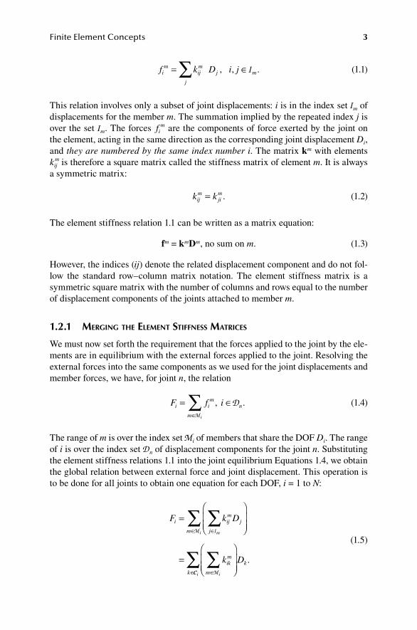
(1.1)
This relation involves only a subset of joint displacements: i is in the index set Im of displacements for the member m. The summation implied by the repeated index j is over the set Im. The forces fi
m are the components of force exerted by the joint on the element, acting in the same direction as the corresponding joint displacement Di, and they are numbered by the same index number i. The matrix km with elements kij
m is therefore a square matrix called the stiffness matrix of element m. It is always a symmetric matrix:
k kij
mjim= .
(1.2)
The element stiffness relation 1.1 can be written as a matrix equation:
fm = kmDm, no sum on m. (1.3)
However, the indices (ij) denote the related displacement component and do not fol-low the standard row–column matrix notation. The element stiffness matrix is a symmetric square matrix with the number of columns and rows equal to the number of displacement components of the joints attached to member m.
1.2.1 Merging the eleMent StiffneSS MatriceS
We must now set forth the requirement that the forces applied to the joint by the ele-ments are in equilibrium with the external forces applied to the joint. Resolving the external forces into the same components as we used for the joint displacements and member forces, we have, for joint n, the relation
F f ii im
n
m i
= ∈∈
∑ , .DM
(1.4)
The range of m is over the index set Mi of members that share the DOF Di. The range of i is over the index set Dn of displacement components for the joint n. Substituting the element stiffness relations 1.1 into the joint equilibrium Equations 1.4, we obtain the global relation between external force and joint displacement. This operation is to be done for all joints to obtain one equation for each DOF, i = 1 to N:
F k D
k
i ijm
j
jm
ikm
mk
mi
i
=
=
∈∈
∈∈
∑∑
∑
IM
MCCi
Dk∑ .
(1.5)

4 The Finite Element Method for Mechanics of Solids with ANSYS Applications
The summation on k in the second term is over the set Ci of those DOFs that are con-nected to the ith DOF by some member, that is, the connectivity of the structure. By definition, no two joints share the same Fi or Di, and the total number of such force and displacement components is N, that is, i = 1 to N.
The summation on k in the last term can be extended to the full range of displacements,
F K Di ik k
k
N
==
∑1
,
(1.6)
by defining Kik = 0 for those k such that Di and Dk are not connected by any member:
Kk k
kik
ikm
i
m
i
i=∈
∉
∈∑ for
for
C
C
M
,
.0
(1.7)
Then, in matrix notation,
F = KD (1.8)
This summation of the element stiffness matrices is called merging of the matrices to form the global stiffness matrix. In the global N × N stiffness matrix K with terms Kik, the index i becomes the row number and the index k becomes the column num-ber of the term.
In Equation 1.7, we are merely adding together all of the terms with common indices from each of the element matrices. We can start by setting all of the terms in the global stiffness matrix K to zero. We then take any one element and add all of the terms from the element stiffness matrix directly into the global stiffness matrix at the appropriate location. Then we go to the next element and repeat the addition of terms from the element stiffness matrix into the global stiffness matrix. This is the process that gave rise to the terminology “merging the stiff-ness matrices.” It is an efficient numerical method for forming the global stiffness matrix. Henceforth, when we indicate a summation of element stiffness matrices, the summation will be understood to mean that element stiffness matrices are merged.
The external forces F consist of the externally applied loads and reactions and the inertial forces. If we approximate the inertial forces by lumping the mass at the joints, the inertial force is (–miDi), no sum on i, for each DOF. The general form of Equation 1.8 including inertial forces is
F MD KD− = (1.9)
where M is a diagonal matrix with the lumped masses mi on the diagonal.
Finite Element Concepts 5
1.2.2 augMenting the eleMent StiffneSS Matrix
It is sometimes helpful to visualize geometrically the process of forming the global stiffness matrix K from the element stiffness matrices. One can imagine that each element stiffness matrix is increased in size to match the global stiffness by inserting zero terms for all terms, other than those terms corresponding to the indices i and j occurring in the element array kij
m, to obtain an N × N element matrix k̂ijm. Equation
1.7 then expresses the ordinary matrix addition:
K k= ∑ ˆ ,m
m
(1.10)
where the summation is over the totality of elements and k̂m is the element matrix augmented by zeros. This has several advantages conceptually. One may think of each element stiffness matrix as written on a sheet of paper with the terms kij
m entered into the row and column of the global array as dictated by indices i and j. The sheets of paper are laid on top of one another and the elements are added that lie in the same position. However, this is not a good plan for computations because it involves manipulating a lot of zeros.
1.2.3 StiffneSS Matrix iS Banded
The geometrical concept of merging the element stiffness matrices is also helpful in understanding the banded nature of the global stiffness matrix. If we are forming the row of K corresponding to say F1, then the only elements that will contribute terms to this row are those attached to the joint having the DOF D1, and the only terms that those elements can contribute to K will be those for the columns corresponding to the displacements of the other DOFs associated with those elements. Consequently, only those terms in that row that are contributed by the elements sharing the DOF D1 can be nonzero. Beyond a certain column number, all of the remaining terms of the row F1 are zero. Thus, the nonzero terms are confined to a band emanating from the diagonal elements of K. By numbering the joint displacements judiciously, we can minimize the width of this band and confine the nonzero terms to a relatively small band around the diagonal of K.
1.3 the energy Method
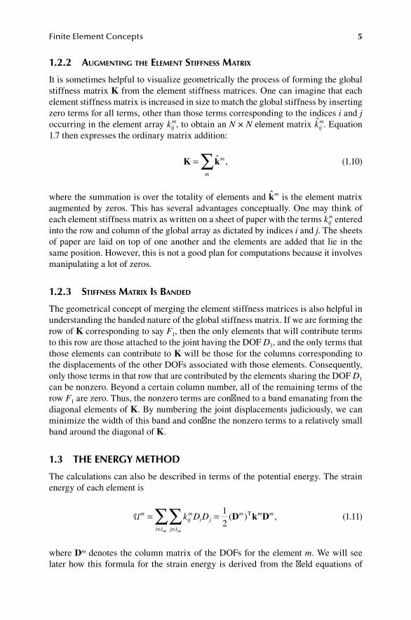
The calculations can also be described in terms of the potential energy. The strain energy of each element is
UII
mijm
i jm m m
ji
k D D
mm
= =∈∈
∑∑ 12
( ) ,D k DT
(1.11)
where Dm denotes the column matrix of the DOFs for the element m. We will see later how this formula for the strain energy is derived from the field equations of
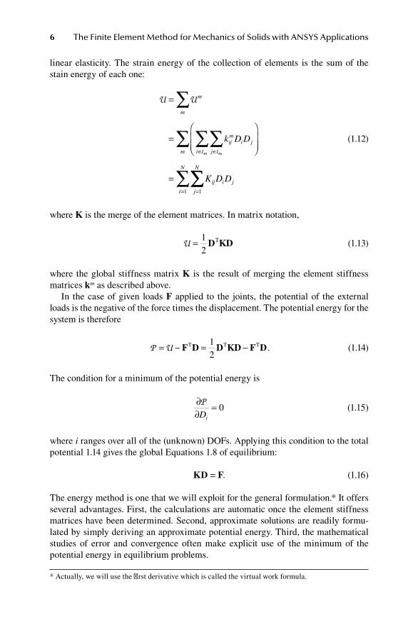
6 The Finite Element Method for Mechanics of Solids with ANSYS Applications
linear elasticity. The strain energy of the collection of elements is the sum of the stain energy of each one:
U U
II
=
=
=
∑
∑∑∑∈∈
=
m
m
ijm
i j
jim
ij i j
j
N
k D D
K D D
mm
1
∑∑∑=i
N
1
(1.12)
where K is the merge of the element matrices. In matrix notation,
U = 1
2D KDT
(1.13)
where the global stiffness matrix K is the result of merging the element stiffness matrices km as described above.
In the case of given loads F applied to the joints, the potential of the external loads is the negative of the force times the displacement. The potential energy for the system is therefore
P U= − = −F D D KD F DT T T1
2.
(1.14)
The condition for a minimum of the potential energy is
∂∂
PDi
= 0
(1.15)
where i ranges over all of the (unknown) DOFs. Applying this condition to the total potential 1.14 gives the global Equations 1.8 of equilibrium:
KD = F. (1.16)
The energy method is one that we will exploit for the general formulation.* It offers several advantages. First, the calculations are automatic once the element stiffness matrices have been determined. Second, approximate solutions are readily formu-lated by simply deriving an approximate potential energy. Third, the mathematical studies of error and convergence often make explicit use of the minimum of the potential energy in equilibrium problems.
* Actually, we will use the first derivative which is called the virtual work formula.

Finite Element Concepts 7
The energy method can be extended to explicitly include the inertial forces by introducing the kinetic energy. If the mass is lumped at a node point (joint), the kinetic energy associated with Dj is
Tj j j jm D D= 1
2 , ( ).no sum
(1.17)
The total kinetic energy of the system is the sum over the number of DOFs:
T T= ∑ j
j
.
(1.18)
Combining 1.17 and 1.18, we find
T = 1
2 D MDT , (1.19)
where the global mass matrix is the result just a diagonal matrix consisting of the individual lumped masses. The equations of motion can be derived from Lagrange’s equations
ddt D D Dj j j
∂∂
∂∂
∂∂
T T P
− = − .
(1.20)
this leads to the general equations of motion for the discrete system:
MD KD F + = (1.21)
This is a set of linear ordinary differential equations that can be solved by standard methods. However, because of the banded nature of M and K, special techniques can be used to reduce the computational effort.
1.4 truSS exaMple
A truss is a collection of axial force members that are joined at the ends in such a way that there is no restraint on the relative rotation of the members at the joint. Each member can be considered an element. The joints are the nodes. The components of displacement of the joints are the degrees of freedom of the structure.
Let us consider the truss shown in Figure 1.1, which has three elements and four nodes numbered as shown. The DOFs are labeled as shown in Figure 1.2. In this case, the total number of DOFs is N = 8. The forces exerted on the elements by the nodes are shown in Figure 1.3, with positive directions as shown.

8 The Finite Element Method for Mechanics of Solids with ANSYS Applications
The force–displacement relations for member 1 are
f k D k D k D k D
i
i i i i i1
11
1 21
2 71
7 81
8
1 1 1 2
= + + +
∈ =
,
, ( , ,I I 77 8, ),
(1.22)
or
f k Di ij j
j
1 1
1
=∈
∑I
.
(1.23)
4L
4
2
3
3
y
x
2
1
1
3L 4L
fIgure 1.1 Truss example.
D4
D1
D2
D7
D8
D5D3
D6
1
123
32 4
y
x
fIgure 1.2 Degrees of freedom for truss.
f81
f11
f21
f12
f52
f62
f33
f43
f22
f13
f23
f71
12
111
43
32
yx
fIgure 1.3 Element forces.

Finite Element Concepts 9
For member 2:
f k D ii ij j
j
2 22
2
1 2 5 6= ∈ =∈
∑ , , ( , , , ).I
I I2
(1.24)
For member 3:
f k D ii ij j
j
3 33
3
1 2 3 4= ∈ =∈
∑ , , ( , , , ).I
I I3
(1.25)
The forces exerted by the external world and by the elements on the nodes are shown in Figure 1.4. The sign convention is that fi
m is in the positive coordinate direction on the element and therefore in the negative coordinate direction on the joint. The equilibrium of forces for node 1 requires that
F f f f f ii i i i im= + + = ∈ = =1 2 3
1 11 2 1 2 3, , ( , ), ( , , ).D D M1
mm∈∑
M1
(1.26)
The equilibrium of forces for node 2 requires that
F f ii im
m
= ∈ = =∈
∑ , , ( ), ( , ).D M DM
2 2 23 3 42
(1.27)
The equilibrium of forces for node 3 requires that
F f ii im
m
= ∈ = =∈
∑ , , ( ), ( , ).D M DM
3 3 32 5 63
(1.28)
The equilibrium of forces for node 4 requires that
432
1
F4 F6 F8
F7
F5
F1
F2
F3
43
33 5
2
62 7
1
81
11
212
2
12
13
23
fIgure 1.4 Forces on nodes.

10 The Finite Element Method for Mechanics of Solids with ANSYS Applications
F f ii im
m
= ∈ = =∈
∑ , , ( ), ( , ).D M DM
4 4 41 7 84
(1.29)
Substitution of the force–displacement relations for the elements provides the force–displacement relations for the assembled structure. For example,
F k D k D k D k D
k D k D k
1 111
1 121
2 171
7 181
8
112
1 122
2 1
= + + +
+ + + 552
5 162
6
113
1 123
2 133
3 143
4
D k D
k D k D k D k D
+
+ + + + .
(1.30)
Adding the common factors for each DOF (merging the stiffness matrices) gives eight force–displacement relations. For the first DOF,
F1 = K11D1 + K12D2 + K13D3 + K14D4 + K15D5 + K16D6 + K17D7 + K18D8, (1.31)
where
K k k k
K k k k
K k
K
11 111
112
113
12 121
122
123
13 133
14
= + +
= + +
=
==
=
=
=
=
k
K k
K k
K k
K k
143
15 152
16 162
17 171
18 181 .
(1.32)
For the third DOF, occurring at node 2,
F f k D k D K D k D3 33
313
1 323
2 333
3 343
4= = + + + . (1.33)
The connectivity sets for the DOFs are
C C1 21 2 3 4 5 6 7 8 1 2 3 4 5= =( , , , , , , , ), ( , , , , , 66 7 8 1 2 3 4 1 2 3 4
1
3 4
5
, , ), ( , , , ), ( , , , ),
(
C C
C
= =
= ,, , , ), ( , , , ), ( , , , ),2 5 6 1 2 5 6 1 2 7 86 7 8C C C= = = (( , , , ).1 2 7 8 (1.34)

Finite Element Concepts 11
In particular, there is no element connecting DOFs 3 and 4 to DOFs 5, 6, 7, and 8. Therefore, K35 = K36 = K37 = K38 = 0, and so forth.
We still have to analyze the truss element in order to determine the element stiff-ness matrices. Each member may be inclined to the x-axis by an angle θ as shown in Figure 1.5. For end a, let Xa and Ya be the components of the member force fa. Let Ua and Va denote the components of axial displacement Da. A similar notation is used at end b.
Let α = cosθ and β = sinθ. Then, Xa = α fa and Ya=β fa. The axial displacement of end a is Da = αUa + βVa. A similar notation is used for end b. Using Equations 1.44 and 1.45, we find the stiffness relation for the element*:
X
Y
X
Y
AEl
a
a
b
b
=
− −− −
−
αα αβ αα αβαβ ββ αβ ββ
ααα αβ αα αβαβ ββ αβ ββ
−− −
U
V
U
V
a
a
b
b
.
(1.35)
For the truss shown in Figure 1.1, Equation 1.35 applies to each member with the appropriate values of α and β. Remember that angle θ is measured counterclockwise from the x-axis in each case. For the case when A and E are the same for all elements, the element stiffness matrices are as follows:
k1 =
+ + − −+ + − −− − + +− − + +
AE
L8 2
1 1 1 11 1 1 11 1 1 11 1 1 1
D D D D1 2 7 8
.
(1.36)
* ANSYS element LINK1.
Ya, Va
Yb, Vb
Xb, Ub
Xa, Ua
a
b
θ
fIgure 1.5 Truss element.

12 The Finite Element Method for Mechanics of Solids with ANSYS Applications
k2 = + −
− +
AEL
D D D D
4
0 0 0 00 1 0 10 0 0 00 1 0 1
1 2 5 6
..
(1.37)
k3 =
+ − − +− + + −
− + + −+ −
AEL125
9 12 9 1212 16 12 16
9 12 9 1212 16 −− +
12 16
1 2 3 4D D D D
.
(1.38)
Merging the three element stiffness matrices gives the global stiffness matrix:
K =
+ − + − − −
−
AE
L
9125
1
8 2
12125
1
8 2
9125
12125
0 01
8 2
1
8 2
121225
1
8 2
16125
14
1
8 2
12125
16125
014
1
8 2
1
8 2
9125
+ + + − − − −
− 112125
9125
12125
0 0 0 0
12125
16125
12125
16125
0 0 0 0
0
−
− −
00 0 0 0 0 0 0
014
0 0 014
0 0
1
8 2
1
8 20 0 0 0
1
8 2
1
8 2
1
8 2
1
8 20 0
−
− −
− − 00 01
8 2
1
8 2
D D D D D D D D1 2 3 4 5 6 7 8
.
(1.39)
The global stiffness matrix has zero determinant so Equation 1.8 does not have a unique solution for given loads F. This is to be expected because the unsupported structure allows rigid translation and rotation and sometimes collapse as a mecha-nism. If the supported structure can act as a mechanism, it is said to be kinematically unstable.
Using the condition of zero displacement at nodes 2, 3, and 4, we find the equilib-rium equations for the supported structure:

Finite Element Concepts 13
AEL
1
8 2
9125
1
8 2
12125
1
8 2
12125
1
8 2
14
16125
+ −
− + +
=
U
V
X
Y1
1
1
1
.
(1.40)
The coefficient matrix is called the reduced stiffness matrix.The joint displacement can now be calculated for given external forces X1 and Y1
by solving Equation 1.40. For Y1 = 0,
U
X LAE
VX LAE1
11
16 2397 101835= =. , . .
(1.41)
This example may be used as a test problem (Section 15.3).
1.5 axIally loaded rod exaMple
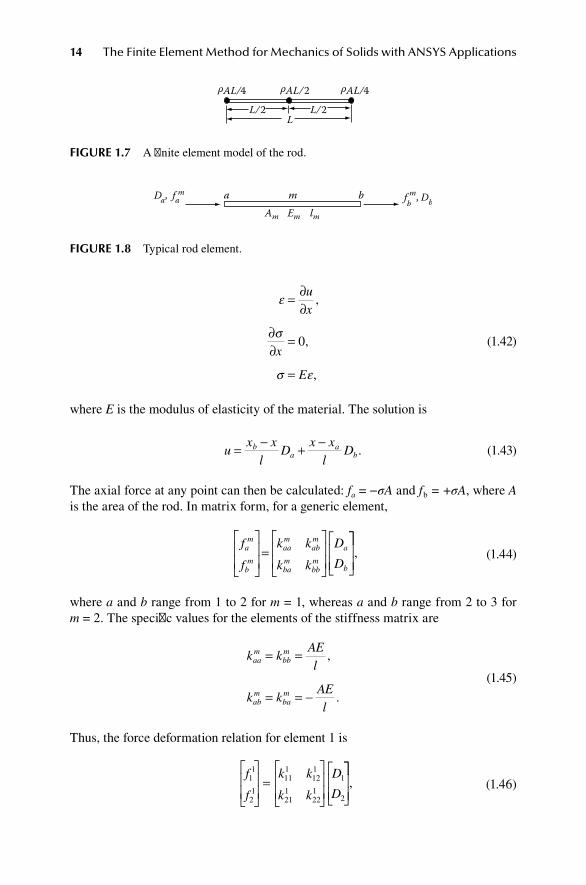
Next, let us consider another simple example that illustrates the ideas of the direct stiffness formulation. A straight rod is loaded by a force applied to one end and supported at the other end (Figure 1.6). The solution of the static problem is trivial, but the matrix formulation may still be useful if additional loads are applied at various points along the rod, or if the material properties vary along the rod. The problem is not so trivial if the loads vary with time and inertial forces are included.
We will formulate approximate equations governing the motion of the rod by using a finite element model. To this end, we divide the rod into of a number of ele-ments. Suppose, for example, we use two elements that are joined at the midpoint of the rod (Figure 1.7). One-half of the mass of each element is lumped at the joint at the end of the element as a first approximation for the inertial forces. For a more accurate solution, one simply increases the number of elements, tending to the exact solution as the number of elements tends to infinity.
The axial (x direction) displacement at each point is denoted by Di, i = 1, 2, 3. The contact forces on element n are denoted by fi
n, where i takes on the values of the joint numbers bounding the element (Figure 1.8). The element properties are approxi-mated as uniform over each element. This may require a larger number of elements for a satisfactory analysis if the properties are varying rapidly.
We can analyze the stress state for each massless element. The equations of linear elasticity for the element are
x
L
P A, E, ρ
fIgure 1.6 Axial force applied to a rod.
14 The Finite Element Method for Mechanics of Solids with ANSYS Applications
ε
σ
σ ε
= ∂∂
∂∂
=
=
ux
x
E
,
,
,
0
(1.42)
where E is the modulus of elasticity of the material. The solution is
u
x xl
Dx x
lDb
aa
b= − + −.
(1.43)
The axial force at any point can then be calculated: fa = −σA and fb = +σA, where A is the area of the rod. In matrix form, for a generic element,
f
f
k k
k k
D
Dam
bm
aam
abm
bam
bbm
a
b
=
,
(1.44)
where a and b range from 1 to 2 for m = 1, whereas a and b range from 2 to 3 for m = 2. The specific values for the elements of the stiffness matrix are
k kAEl
k kAEl
aam
bbm
abm
bam
= =
= = −
,
.
(1.45)
Thus, the force deformation relation for element 1 is
f
f
k k
k k
D
D11
21
111
121
211
221
1
2
=
,
(1.46)
ρAL/4
L/2L
L/2
ρAL/4 ρAL/2
fIgure 1.7 A finite element model of the rod.
a bm fbm, Db
Da, fam
lmAm Em
fIgure 1.8 Typical rod element.

Finite Element Concepts 15
and for element 2,
f
f
k k
k k
D
D22
32
222
232
322
332
2
3
=
,
(1.47)
with the terms kabm defined as stated above. Notice that no element index is required
for the displacement components because they are the displacements of the joint to which the element is attached. And the indices on kab
m match the displacement and force components, not the location in the element stiffness matrix.
The equilibrium of forces for the joint j is expressed by
F m D fj j j jm
m
− = ∑ , (no sum on j), (1.48)
where Fj is the external load acting on the joint, mj is the mass that has been lumped at the joint, a superposed dot indicates the time derivative, and the summation extends over the elements that are connected to the joint j. Substitution of the force–deforma-tion relations 1.46 and 1.47 into the equilibrium relation 1.48 with l = L/2 leads to the global equation of equilibrium, relating the external loads to the joint displacements:
ρ
ρ
ρ
AL
AL
AL
D
D
D
40 0
02
0
0 04
1
2
33
2 2 0
2 4 2
0 2 2
+
−
− −
−
AEL
AEL
AEL
AEL
AEL
AEL
AEEL
D
D
D
F
F
F
=
1
2
3
1
2
3
.
(1.49)
Alternatively, using 1.33, 1.14, and 1.20, we obtain once more the governing Equations 1.49 by the energy method. In matrix notation,
MD KD F + = . (1.50)
At each joint, either Fj or Dj is given and the equations have to be solved for the other quantity. In the particular case shown in Figure 1.6, D3 = 0. There are therefore three equations in three unknowns (D1, D2, F3), where F3 is the reaction at the support. It is convenient to divide the relations into two sets. First, solve for the unknown displace-ments corresponding to the given forces:
ρ
ρ
AL
AL
D
D
AEL
AE4
0
02
2 21
2
+−
LLAEL
AEL
D
DP
−
=
2 4 01
2
. (1.51)
16 The Finite Element Method for Mechanics of Solids with ANSYS Applications
Then, solve for the reactions at the joints with zero displacement:
0 0 021
2
1
2
+ −
D
DAEL
D
D
= [ ]F3 . (1.52)
The zero terms are shown for completeness. If the inertial loads are neglected ( D1 0= , D2 0= ), then the solution to Equation 1.51 is
D
D
PLAE
1
2 221
=
. (1.53)
We will consider methods of solution of the equations later. At this time, we sim-ply note that the problem is reduced to a set of linear ordinary differential equa-tions in time, or to a set of linear algebraic equations if the inertial forces are neglected.
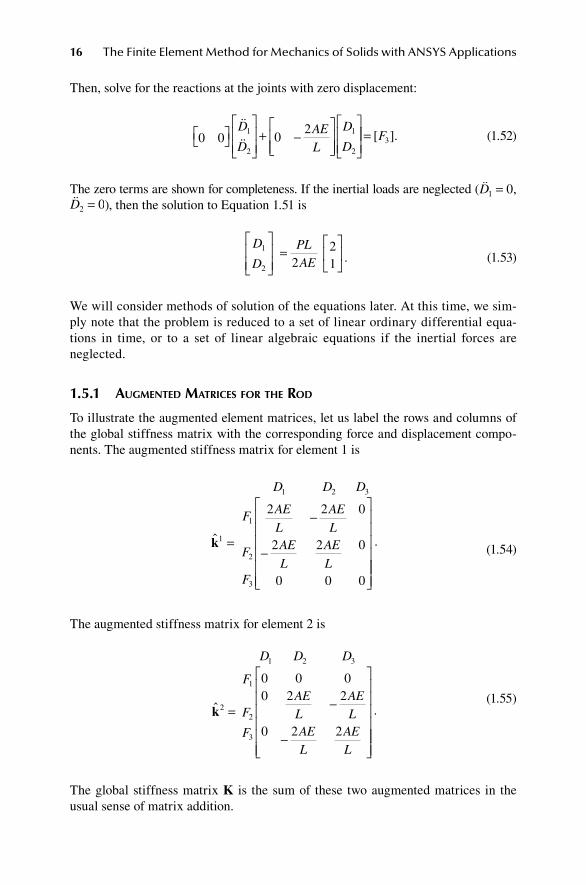
1.5.1 augMented MatriceS for the rod
To illustrate the augmented element matrices, let us label the rows and columns of the global stiffness matrix with the corresponding force and displacement compo-nents. The augmented stiffness matrix for element 1 is
k̂1
1
2
3
2 2 0
2 2 0
0 0 0
=
−
−
F
F
F
AE
L
AE
LAE
L
AE
L
D D D1 2 3
.
(1.54)
The augmented stiffness matrix for element 2 is
k̂2
1
2
3
0 0 00 2 2
0 2 2
= −
−
F
F
F
AEL
AEL
AEL
AEL
D D D1 2 3
.
(1.55)
The global stiffness matrix K is the sum of these two augmented matrices in the usual sense of matrix addition.

Finite Element Concepts 17
K k= ∑ ˆ m
m
.
(1.56)
However, I emphasize again that this is not a practical method for real engineering problems because of the large number of zeros that must be handled.
1.5.2 Merge of eleMent MatriceS for the rod
We will now illustrate the process of forming the global stiffness matrix by merging the element matrices:
K k= ∑ m
m
.
(1.57)
First, construct the global stiffness matrix with all terms equal to zero:
K =
FF
F
D D D
1
2
3
1 2 3
0 0 00 0 00 0 0
.
(1.58)
After merging the stiffness matrix of element 1, the global stiffness matrix is
K =
−
−
F
F
F
AEL
AEL
AEL
AEL
1
2
3
2 20
2 20
0 0 0
DD D D1 2 3
.
(1.59)
After merging the stiffness matrix of element 2 to this matrix, the final global stiff-ness matrix is
K =
−
− −
−
F
F
F
AEL
AEL
AEL
AEL
AEL
AEL
AEL
1
2
3
2 20
2 4 2
02 2
D D D1 2 3
.
(1.60)

18 The Finite Element Method for Mechanics of Solids with ANSYS Applications
The symbols Di and Fi are written along side of the columns and rows in order to identify the related component of force and displacement. They are only labels to assist in the merge process. A computer program will always assume that the third row corresponds to F3 for example, without any labels. If we are forming the row of K corresponding to say F1, then the only elements that will contribute terms to this row are those attached to joint 1, and the only terms that they can contribute will be those for the columns corresponding to the displacements of the other end of the element. In this simple example, only element number one can contribute to the row for F1, and it is connected only to joints 1 and 2, so the only entries will be to the columns for D1 and D2, regardless of the number of elements used to model the rod. There is no contribution to the term (F1, D3), or any column beyond D3, which are therefore zero, even if there were more elements. Starting with the diagonal element and counting to the right, there will be only two nonzero elements in each row. This is the called the half bandwidth of K.
1.6 force Method
In the preceding formulation, the joint displacements are the fundamental unknowns. Before stored-program digital computers became available, it was more common to think of the element forces as fundamental unknowns. For any assemblage of rods, the resultant axial for each rod was regarded as the fundamental unknown. The difference in view point can be made clear by an example. Let us consider, for example, the truss shown Figure 1.9. All members have area A and modulus E.
Let D1 and D2 denote the displacements in the direction of the applied forces F1 and F2. Let εi denote the increment in length of element i. Let Si denote the tensile force for element i. The equilibrium relations for the loaded joint are
−
− − −
=
1
2
0 35
1
2
1 45
1
2
3
S
S
S
FF
F1
2
or BS = F. (1.61)
4L
FXFY
4L3L
123
fIgure 1.9 Statically indeterminate truss.

Finite Element Concepts 19
The geometric relations between extensions of the elements and the joint displace-ments are
ε
ε
ε
1
2
3
1
2
1
2
0 135
45
=
− −
−
−
D
D1
2
or ε = AD. (1.62)
The constitutive relations between the extensions of the elements and the axial forces are
ε
ε
ε
1
2
3
4 2 0 0
0 4 0
0 0 5
=
LAE
LAE
LAE
S
S
S
1
2
3
or ε = fS (1.63)
where f is the flexibility matrix of the structure.The theorem of virtual work that we will develop later states that the internal
work equals the external work, STε = FTD, for every equilibrium system (S, F) and every compatible system (ε, D). That is, STAD = STBTD for every S and D. Therefore, A = BT, as the explicit example shows.
In general, there will be s stress parameters and d displacement parameters. The matrix B is d × s. If s = d, the equilibrium equations can be solved for S unless the det B = 0. If the determinant is zero, the system is kinematically unstable. If d > s, then S is overdetermined. This implies the existence of displacement fields with zero generalized strains, and the structure is unstable. If d < s, as in the example, the equi-librium Equations 1.61 have more unknowns Si than equations, and the structure is said to be statically indeterminate. The general solution to 1.61 is then of the form
S = b0F + b1R. (1.64)
The elements of R are s – d = r in number and are called redundant forces. In this example, there is one redundant force R1. We can choose the force in member 3 as the redundant (or any other member): S3 = R1. Then, we find from 1.61 that
b b0 1
2 0
1 10 0
3 2 5
7 51
=−
−
= −
,/
/ .
(1.65)

20 The Finite Element Method for Mechanics of Solids with ANSYS Applications
The coefficient matrices are such that
Bb0 = 1 (1.66)
and
Bb1 0= . (1.67)
Since A = BT, we have from 1.62 and 1.67 the compatibility relation
b1T 0εε = . (1.68)
Substituting 1.63 into 1.68,
c0F + c1R = 0 (1.69)
where
c b fb c b fb0 1 0 1 1 1= =T T, . (1.70)
Therefore,
R c c F= − −11
0 . (1.71)
Substituting 1.71 into 1.64 yields the formula for solution by the redundant force method:
S = bF, (1.72)
where
b b b c c= − −0 1 1
10. (1.73)
There exists standard algorithms for constructing the solution 1.64 of the equi-librium equations, and the redundant force method is a viable procedure for stress analysis provided someone has developed a computer code to automate the calculations.
It may be noticed that the stiffness method, which was introduced first, avoided altogether the question of redundant forces. The two methods are, however, equiva-lent for the same structural model. The stiffness formulation can be recovered by eliminating S and ε from Equations 1.61 to 1.63:
KD = F (1.74)

Finite Element Concepts 21
where
K = Bf –1BT. (1.75)
This K is the reduced stiffness matrix that one obtains after applying the displace-ment boundary conditions.
1.7 other Structural coMponentS
1.7.1 Space truSS
In general, elements of the truss may have any spatial orientation with respect to the global coordinate system. The axial displacement at each end is then resolved into components along the three coordinate axes, so there are 3 DOFs at each end.
If the numbering scheme follows that of Figure 1.10, the DOFs associated with node i will be DT = [D3i−2D3i−1D3i] as shown in Figure 1.10. The corresponding ele-ment and nodal forces are numbered in the same manner: FT = [F3i−2F3i−1F3i]. For element m that connects nodes 1 and 2, we have the force–displacement relation:
f
f
f
f
f
f
A EL
m
m
m
m
m
m
m m
m
1
2
3
4
5
6
=
αα αβ αγ α αβ αγ
αβ β βγ αβ β βγ
αγ βγ γ αγ βγ γ
2 2
2 2
2 2
− − −− − −− − −
−αα αβ αγ α αβ αγ
αβ β βγ αβ β βγ
αγ βγ γ αγ βγ γ
2 2
2 2
2 2
− −− − −− − −
D
D
D
D
D
D
1
2
3
4
5
6
, (1.76)
where α, β, and γ are the direction cosines of the rod. An assembly of such elements is a three-dimensional truss. Each joint is a node with 3 DOFs.
1.7.2 BeaMS and fraMeS
In general, a rod element may be subject to bending and twist as well as axial defor-mations and may be called a rod, beam, or beam–column element. We will suppose
D3i-2D3i-1
D3i
i
x1x2
x3D1
D2
D3
D4
D5
D6
m
1
2
fIgure 1.10 Space truss element.
22 The Finite Element Method for Mechanics of Solids with ANSYS Applications
here that all loads are applied at the ends of the beam element. There are 6 DOFs at each end: 3 components of displacement and 3 components of rotation. The first three being components of displacement along the coordinate axes, and the second three being rotations about the axes. By elementary mechanics of materials, we can establish the relation between the generalized forces on the ends of the rod and the generalized displacements of the ends of the rod. An assembly of such elements is a three-dimensional space frame. Each joint is a node with 6 DOFs.
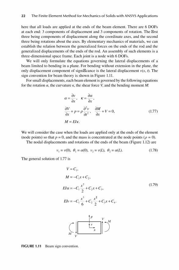
We will only formulate the equations governing the lateral displacements of a beam limited to bending in a plane. For bending without extension in the plane, the only displacement component of significance is the lateral displacement v(x, t). The sign convention for beam theory is shown in Figure 1.11.
For small displacements, each beam element is governed by the following equations for the rotation α, the curvature κ, the shear force V, and the bending moment M:
αα
ρ
κ
κ= ∂∂
= ∂∂
∂∂
+ = ∂∂
∂∂
+ =
=
vx x
Vx
pv
t
Mx
V
M EI
, ,
, ,
.
2
20
(1.77)
We will consider the case when the loads are applied only at the ends of the element (node points) so that p = 0, and the mass is concentrated at the node points (ρ = 0).
The nodal displacements and rotations of the ends of the beam (Figure 1.12) are
v1 = v(0), θ1 = α(0), v2 = v(L), θ2 = α(L). (1.78)
The general solution of 1.77 is
V C
M C x C
EI Cx
C x C
EIv Cx
Cx
=
= − +
= − + +
= − +
1
1 2
1
2
2 3
1
3
2
2
6
,
,
,α
22
3 42+ +C x C .
(1.79)
Mp
v
xM
V
V
fIgure 1.11 Beam sign convention.

Finite Element Concepts 23
Therefore,
C EIv
C EI
CEI
Lv
EIL
EI
Lv
EIL
4 1
3 1
2 2 1 1 2 26 4 6 2
=
=
= − − + −
,
,θ
θ θθ
θ θ
2
1 3 1 2 1 3 2 2 212 6 12 6
CEI
Lv
EI
L
EI
Lv
EI
L= − − + − .
(1.80)
The ends of the beam element are nodes in the finite element analysis. The sign convention for nodal forces is shown in Figure 1.13. The forces and moments on the ends of the rod are
f1 = –V(0), m1 = –M(0), f2 = V(L), m2 = M(L). (1.81)
Therefore,
f
m
f
m
EI
L
EI
L
EI
L
EI
L1
1
2
2
3 2 3 2
12 6 12 6
6
=
−
EEI
L
EIL
EI
L
EIL
EI
L
EI
L
EI
L
EI
LEI
2 2
3 2 3 2
4 6 2
12 6 12 6
6
−
− − −
LL
EIL
EI
L
EIL
v
v
2 2
1
1
2
2 6 4−
θ
θθ2
. (1.82)
θ2θ1
2
v2v1
EI
L
1
y
x
fIgure 1.12 Definition of nodal DOF.
m2
2
f2f1
1
m1y
x
fIgure 1.13 Generalized forces on a beam element.
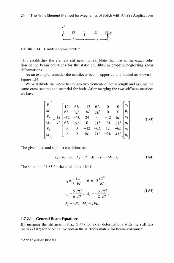
24 The Finite Element Method for Mechanics of Solids with ANSYS Applications
This establishes the element stiffness matrix. Note that this is the exact solu-tion of the beam equations for the static equilibrium problem neglecting shear deformations.
As an example, consider the cantilever beam supported and loaded as shown in Figure 1.14.
We will divide the whole beam into two elements of equal length and assume the same cross section and material for both. After merging the two stiffness matrices we have
F
M
F
M
F
M
EI
L
L L1
1
2
2
3
3
3
12 6 12 6 0
=
− 006 4 6 2 0 0
12 6 24 0 12 66 2 0 8 6 20 0
2 2
2 2 2
L L L LL L
L L L L L
−− − −
−−112 6 12 6
0 0 6 2 6 42 2
1
1
– L LL L L L
v
v
−−
θ
22
2
3
3
θ
θ
v
.
(1.83)
The given load and support conditions are
v3 = θ3 = 0, F1 = P, M1 = F2 = M2 = 0. (1.84)
The solution of 1.83 for the conditions 1.84 is
vPLEI
PLEI
vPLEI
PLEI
F
1
3
1
2
2
3
2
2
3
83
2
56
32
= = −
= = −
, ,
, ,
θ
θ
== − =P M PL, .3 2
(1.85)
1.7.2.1 general Beam equationsBy merging the stiffness matrix (1.44) for axial deformations with the stiffness matrix (1.82) for bending, we obtain the stiffness matrix for beam–columns*:
* ANSYS element BEAM3.
P
1 EI 2 EI 3
LL
fIgure 1.14 Cantilever beam problem.
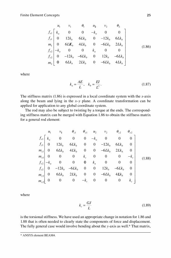
Finite Element Concepts 25
f
f
m
f
f
m
k k
k Lk k Lk
L
x
y
x
y
a a
b b b b
1
1
1
2
2
2
0 0 0 0
0 12 6 0 12 6
0 6
−−
KK Lk Lk Lk
k k
k Lk k Lk
b b b b
a a
b b b b
4 0 6 2
0 0 0 0
0 12 6 0 12 6
−−
− − −00 6 2 0 6 4
1 1 1
Lk Lk Lk Lk
u v u
b b b b−
θ 22 2 2v θ
(1.86)
where
k
AEL
kEI
La b= =, .
3
(1.87)
The stiffness matrix (1.86) is expressed in a local coordinate system with the x-axis along the beam and lying in the x–y plane. A coordinate transformation can be applied for application to any global coordinate system.
The rod may also be subject to twisting by a torque at the ends. The correspond-ing stiffness matrix can be merged with Equation 1.86 to obtain the stiffness matrix for a general rod element:
f
f
m
m
f
f
m
m
k k
k Lk
x
y
z
x
x
y
z
x
a a
b b
1
1
1
1
2
2
2
2
0 0 0 0 0 0
0 12 6 0 0
−−112 6 0
0 6 4 0 0 6 2 0
0 0 0 0 0 0
0 0
k Lk
Lk Lk Lk Lk
k k
k
b b
b b b b
c c
a
−−
− 00 0 0 0
0 12 6 0 0 12 6 0
0 6 2 0 0 6 4
k
k Lk k Lk
Lk Lk Lk
a
b b b b
b b b
− − −− LLk
k k
u v
b
c c
0
0 0 0 0 0 0
1
−
11 1 1 2 2 2 2θ θ θ θz x z xu v
(1.88)
where
k
GJLc =
(1.89)
is the torsional stiffness. We have used an appropriate change in notation for 1.86 and 1.88 that is often needed to clearly state the components of force and displacement. The fully general case would involve bending about the y-axis as well.* That matrix,
* ANSYS element BEAM4.
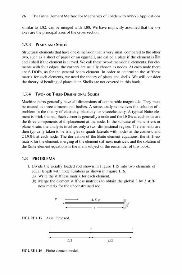
26 The Finite Element Method for Mechanics of Solids with ANSYS Applications
similar to 1.82, can be merged with 1.88. We have implicitly assumed that the x–y axes are the principal axes of the cross section.
1.7.3 plateS and ShellS
Structural elements that have one dimension that is very small compared to the other two, such as a sheet of paper or an eggshell, are called a plate if the element is flat and a shell if the element is curved. We call these two-dimensional elements. For ele-ments with four edges, the corners are usually chosen as nodes. At each node there are 6 DOFs, as for the general beam element. In order to determine the stiffness matrix for such elements, we need the theory of plates and shells. We will consider the theory of bending of plates later. Shells are not covered in this book.
1.7.4 two- or three-diMenSional SolidS
Machine parts generally have all dimensions of comparable magnitude. They must be treated as three-dimensional bodies. A stress analysis involves the solution of a problem in the theory of elasticity, plasticity, or viscoelasticity. A typical finite ele-ment is brick shaped. Each corner is generally a node and the DOFs at each node are the three components of displacement at the node. In the subcase of plane stress or plane strain, the analysis involves only a two-dimensional region. The elements are then typically taken to be triangles or quadrilaterals with nodes at the corners, and 2 DOFs at each node. The derivation of the finite element equations, the stiffness matrix for the element, merging of the element stiffness matrices, and the solution of the finite element equations is the main subject of the remainder of this book.
1.8 proBleMS
1. Divide the axially loaded rod shown in Figure 1.15 into two elements of equal length with node numbers as shown in Figure 1.16. (a) Write the stiffness matrix for each element.(b) Merge the element stiffness matrices to obtain the global 3 by 3 stiff-
ness matrix for the unconstrained rod.
x
L
P A, E, ρ
fIgure 1.15 Axial force rod.
1 2 3
L/2 L/2
fIgure 1.16 Finite element model.

Finite Element Concepts 27
2. Divide the axially loaded rod shown in Figure 1.15 into three elements of equal length. (a) Write the stiffness matrix for each element showing relevant displace-
ment and force numbers.(b) Merge the element stiffness matrices to obtain the global 4 by 4 stiff-
ness matrix for the unconstrained rod. 3. Divide the axially loaded rod (Figure 1.15) into three elements of equal
length.(a) Form the global stiffness matrix, the global mass matrix, and the global
force matrix.(b) Apply the boundary conditions and determine the reduced set of equa-
tions to be solved for displacements, but do not solve the resulting set of equations.
4. The truss shown in Figure 1.17 has A = 1, L = 1, E = 30 × 106, X1 = 100, Y1 = 0. Solve for the nodal displacements using ANSYS and compare with the exact solution. (See Section 15.3.)
5. Consider the bending of a cantilever beam modeled with two elements (Figure 1.18).(a) Determine the global stiffness matrix K by merging the element
matrices.(b) Apply the support conditions to determine the reduced stiffness matrix
K0. 6. The cantilever beam shown Figure 1.18 has a square cross section, h = 2,
w = 1, A = 2, I = 2/3, E = 1000, L = 5, P = 1. Solve the following beam bend-ing problem using ANSYS (see Section 15.4).(a) Print list of UY at each node.(b) Submit list of moments at the right end of each element from an Element
Data Table.
Y1
X1
4L3L
123
2 3 4
1
4L
fIgure 1.17 Truss configuration.
P
1 EI EI
LL
2 3
fIgure 1.18 Bending of a beam.

28 The Finite Element Method for Mechanics of Solids with ANSYS Applications
(c) Submit list of bending stress at the right end of each element from an Element Data Table.
(d) Compare with numerical solution with the exact solution.
referenceS
1. Courant, R., Variational methods for the solution of problems of equilibrium and vibra-tion, Bull. Am. Math. Soc., 49, 1–43, 1943.
2. Strang, G., and G. J. Fix, An Analysis of the Finite Element Method, Prentice-Hall, Inc., Englewood Cliffs, NJ, 1973.
3. Oden, J. T., and J. N. Reddy, An introduction to the Mathematical Theory of Finite Elements, John Wiley, New York, 1976.
4. Oden, J. T., and G. F. Carey, Finite Elements: Mathematical Aspects, Prentice-Hall, Englewood Cliffs, NJ, 1983.
5. Brenner, S. C., and L. R. Scott, The Mathematical Theory of Finite Element Methods, Springer, New York, 3rd ed. 2008.
6. Atluri, S. A., The Meshless Method (MLPG) for Domain & BIE Discretizations, Tech Science Press, Forsyth, GA, 2004.
7. Argyris, J., and S. Kelsey, Energy Theorems and Structural Analysis, Butterworth Scientific Publications, London, 1960.
8. Turner, M. J., R. Clough, H. Martin, and L. Topp, Stiffness and Deflection Analysis of Complex Structures, J. Aero. Sci., 23, no. 9, Sept., 1956, pp. 805–823.
9. Clough, R., The finite element in plane stress, Proc. 2nd ASCE Conf. on Electronic Computation, Pittsburgh, PA, Sept. 1960.
BIBlIography
Cook, R. D., Concepts and Applications of Finite Element Analysis, John Wiley, New York, 1974.
Gallagher, R. H., Finite Element Analysis, Prentice-Hall, Englewood Cliffs, NJ, 1975.Martin, H. C., Introduction to Matrix Methods of Structural Analysis, McGraw-Hill, New York,
1966.Przemieniecki, J. S., Theory of Matrix Structural Analysis, McGraw-Hill, New York, 1968.Zienkiewicz, O. C., The Finite Element Method in Structural and Continuum Mechanics,
McGraw-Hill, London, 1967.

29
2 Linear Elasticity
2.1 BaSIc equatIonS
In this chapter we will summarize the set of differential equations that govern the motion of elastic bodies experiencing small deformations. This set of differential equations, together with the boundary and initial conditions, is a well-posed math-ematical problem that we wish to solve via numerical methods. It is assumed that the reader is familiar with the derivation and use of these relations. They are presented here in rectangular Cartesian components without derivation. Index notation with summation convention is used. English letter indices have the range (1, 2, 3) and Greek letter indices have the range (1, 2).
2.1.1 geoMetry of deforMation
We consider a material body that occupies a region V of space with a boundary S. A particle of material has coordinates xk = (x,y,z) (before deformation) and experi-ences a displacement vector with components uk = (u,v,w) that are functions of the coordinates xk and time t. Extensions and shears of material fibers are determined by the strain tensor, which has components εkm that are related to the components of the displacement vector by
ε km
k
m
m
kk m
ux
ux
u= ∂∂
+ ∂∂
≡12 ( , ).
(2.1)
We will also use the alternate notation:
ε ε ε γ
ε ε ε γ
ε ε ε γ
11 12
22 23
33 31
2
2
2
= =
= =
= =
x xy
y yz
z zx
, ,
, ,
, ..
(2.2)
The extension (normal strain) of a material fiber that is initially along the x1 axis is ε11. The shear (shear strain) of a pair of fibers that are initially along the x1 and x2 axis is γxy = 2ε12. That is, the physical shear is twice the tensor component. Each component ui of the displacement vector is a continuous function of the coordinates xi and the function is continuously differentiable except possibly at isolated points, lines, or surfaces. Any continuous displacement field together with the strain tensor determined by Equation 2.1 is called a compatible system.

30 The Finite Element Method for Mechanics of Solids with ANSYS Applications
2.1.2 Balance of MoMentuM
The state of stress is characterized by the stress tensor with components τkm. The components τkm are functions of the coordinates xk and time t. At each time t the functions are continuous and differentiable in V except possibly at isolated points, lines, or surfaces. The balance of linear momentum is expressed by
∂∂
τρij
ji ix
b u+ = .
(2.3)
The balance of angular momentum is expressed by
τij = τji. (2.4)
We will also use the alternate notation:
τ τ σ τ τ
τ τ σ τ τ
τ τ σ
11 12
22 23
33
= = =
= = =
= =
xx x xy
yy y yz
zz
, ,
, ,
zz zx, .τ τ31 =
(2.5)
Now, consider a closed surface bounding all or part of the material. Let ni denote the components of the unit vector normal to the surface and directed toward the exterior of the body. The components of the force per unit area Ti exerted on the body at the bounding surface by the surrounding material, or by the exterior world, is related to the stress tensor at each point on the surface by
Ti = τijnj. (2.6)
The vector with components Ti is called the stress vector or traction vector. The stress vector is continuous across each interior surface. A smooth stress field τij together with the surface tractions Ti determined by 2.6 is called an equilibrium system.
2.1.3 Virtual work
An alternative statement of the balance of momentum is provided the theorem, or principle, of virtual work. This relation can be derived as follows.
Let ui and εij denote any compatible system. Multiplying 2.3 by ui, summing on i, and integrating by parts gives
Tu A b u u V Vi i i i i ij ijd d dS V V∫ ∫ ∫+ − =( ) .ρ τ ε
(2.7)
Linear Elasticity 31
We have used τij = τji and Ti = τijnj. Equation 2.7 has a physical interpretation: The first term is the work of surface tractions Ti moving through displacements ui and the second is the work of the total body forces. The right side expresses the work of the internal stresses τij, which are in equilibrium with the surface tractions Ti and the total body force. That is, the external work equals internal work for a body in equilibrium. Since the functions ui need not be the actual displacements of the material body, they are called virtual displacements and Equation 2.7 expresses the theorem of virtual work.
We have just proved that any equilibrium system satisfies relation 2.7 for every compatible system. The reverse is also true. Smooth functions τij = τji satisfy the equilibrium equations 2.3 if and only if Equation 2.7 of virtual work holds for all smooth functions.
2.1.4 conStitutiVe relationS
For any stress analysis problem, we must supply a mathematical characterization of the material by specification of the relation between the stress and the strain. The classical theories of materials are elasticity, plasticity, and viscoelasticity. We will consider the theory of elasticity in this chapter. For elastic materials, the stress and strain tensors are related by
τεij
ij
= ∂∂A( )
,εε
(2.8)
where
A( ) .εε = +1
2c lijkm ij km ij ijε ε ε
(2.9)
The term lij = lji is a function of temperature change and the constants cijkm satisfy the following symmetry conditions:
cijkm = cjikm = cijmk = ckmij. (2.10)
Thus,
τij = lij + cijkmεkm. (2.11)
For an isotropic material with linear thermal expansion,
A( ) ( ) ,εε = + −µε ε
λε β εkm km kk kkT
22
(2.12)
and 2.11 simplifies to
τkm = –βTδkm + 2μεkm + λεiiδkm. (2.13)

32 The Finite Element Method for Mechanics of Solids with ANSYS Applications
That is,
lij = –βTδij, (2.14)
and
cijkm = μ(δikδjm + δimδjk) + λδijδkm, (2.15)
where β, μ, and λ are material constants and T is the temperature change. In terms of the shear modulus G, the modulus of elasticity E, the Poisson ratio ν, and the co efficient of linear thermal expansion α,
µν
λν
νβ
αν
λλ µ
ν µ λµ
= =+
=−
=−
+= + =
GE G E
2 12
1 2 1 2
2 2 32
( ), , ,
,(( )
, .1
1 22 2
+−
+ =νν
λ µ ν
(2.16)
The constitutive relations for an isotropic material are simplified if we introduce the deviatoric components of the tensors, which are defined as follows:
s
e
km km ii km
km km ii km
= −
= −
τ τ δ
ε ε δ
13
13
,
.
(2.17)
The constitutive relation 2.13 then becomes
s e
T
km km
kk kk
=
= − +
µ
τ β κε
2
13
,
,
(2.18)
where κ is the bulk modulus,
κ λ µ
ν= + =
−23 3 1 2
E( )
.
(2.19)
The deviatoric components of strain are measures of distortion (γ12 = 2e12 is the shear of the x–y fibers), and the first equation in 2.18 is therefore the constitutive relation for distortion. The quantity εkk is the volumetric strain, and the second equa-tion in 2.18 is the constitutive relation for dilatation relating the mean stress τkk/3 to the volumetric strain. The two relations in 2.18 are equivalent to the single equation 2.13. Constitutive relations for small deformations of isotropic materials that are not

Linear Elasticity 33
elastic can be derived by replacing the simple proportionality in 2.18 with more complicated relations. We will consider two possibilities later when we study vis-coelastic materials and the theory of plasticity.
2.1.5 Boundary conditionS and initial conditionS
Now, consider a closed surface bounding all of the material. Let ni denote the compo-nents of the unit vector normal to the surface and directed toward the exterior of the body. The force per unit area Ti exerted on the body at the surface by the surrounding material, or by the exterior world, is related to the stress tensor at a point on the surface by 2.6:
Ti = τijnj. (2.20)
The external surface of the body consists of two sets of points ST and Su, where the stress vector or the displacement vector must be specified:
T Ti i T= o on S , (2.21)
u ui i u= o on S . (2.22)
For dynamical problems, one must also specify initial conditions:
u u ti iand given in at V = 0. (2.23)
The exact solution to the elasticity problem for a given temperature is a set of func-tions τij, εij, and ui satisfying the differential equations 2.1, 2.3, and 2.11, the bound-ary conditions 2.21 and 2.22, and the initial conditions 2.23.
2.1.6 incoMpreSSiBle MaterialS
If the bulk modulus is very large compared to the shear modulus, a satisfactory solution of the elasticity equations can often be obtained by neglecting the volume change. The mean stress is then determined by the differential equations and the boundary conditions and not by the constitutive relations. The fundamental equa-tions (no temperature change) are
ε ε
τρ
kmk
m
m
kkk
ij
ji
ux
ux
xb u
= +
=
+ =
12
0∂∂
∂∂
∂∂
, ,
ii
km km km ii kmp
,
.τ δ µε λε δ= − + +2
(2.24)
There is one additional equation (εkk = 0) and one additional unknown (p).
34 The Finite Element Method for Mechanics of Solids with ANSYS Applications
2.1.7 plane Strain
There are two very important special cases in which the number of spatial coordi-nates that need to be considered can be reduced from three to two: plane stress and plane strain. For plane strain, εk3 = 0 and all quantities are independent of the x3 coordinate. Then, from 2.13,
τ13 = 0, τ23 = 0, τ33 = –βT + λεθθ, (2.25)
τ β δ µε
νµν
ε δαβ αβ αβ θθ αβ= − + +−
T 221 2
.
(2.26)
From 2.1,
εαβα
β
β
α
= +
12
∂∂
∂∂
ux
u
x.
(2.27)
From 2.3,
∂∂
+ =τ
ραβ
βα αx
b u ,
(2.28)
since the derivatives with respect to x3 are zero.Equations 2.26–2.28 are a set of eight equations in eight unknowns (u1, u2, τ11,
τ22, τ12, ε11, ε22, ε12) that are called the equations of plane strain for an isotropic mate-rial. Such relations can often be used to adequately characterize the deformations of cylindrical bodies with loads and temperature changes that do not vary along the length of the cylinder and where the ends of the cylinder are prevented from under-going axial displacement (ε33 ≡ 0).
The constitutive relations 2.26 can be expressed in the form 2.8 if we redefine A and lαβ as follows.
A( ) ( ) ,εε = +
−+µε ε
νµν
ε εαβ αβ θθ αβ αβ1 22 l
(2.29)
with
lαβ = βTδαβ (2.30)
for plane strain.
2.1.8 plane StreSS
For plane stress, τk3 = 0 and all quantities are independent of x3. From 2.13, it follows that
ε
νµ ν
βν
νεθθ33
1 22 1 1
= −−
−−
( )( )
,T
(2.31)
Linear Elasticity 35
τν
νβ δ µε
µνν
ε δ
ν
αβ αβ αβ θθ αβ= − −−
+ +−
= − −
( )
( )
1 21
221
1 21
T
−−+ + +
−
ν
β δ µ δ δ δ δµν
νδ δ εαβ αθ βφ αφ βθ αβ θφ θφT ( )
21
..
(2.32)
From 2.1,
εαβα
β
β
α
= +
12
∂∂
∂∂
ux
u
x.
(2.33)
From 2.3,
∂∂
τραβ
βα αx
b u+ = .
(2.34)
Equations 2.32–2.34 are, again, a set of eight equations in eight unknowns that are called the equations of plane stress for an isotropic material. Such relations can often be used to adequately characterize the deformations of thin sheets that are loaded only on the edges.
The full equations of elasticity are only approximately satisfied by the plane stress assumptions because there is no solution to the geometric relations 2.1 for u3 cor-responding to the plane stress conditions. The stress and displacement should be viewed as the mean value over the thickness of the sheet. This is often referred to as generalized plane stress.1
The constitutive relations 2.32 can be expressed in form 2.8 if we redefine A and lαβ as follows.
A( ) ( ) , ( )εε = +
−+µε ε
µνν
ε εαβ αβ θθ αβ αβ12 l plane stress
(2.35)
l Tαβ αβ
νν
β δ= − −−
( ). ( )
1 21
plane stress
(2.36)
The equations of plane stress and plane strain have a formal similarity. Keeping μ the same, the plane strain equations 2.26 are transformed into the plane stress relations 2.32 if ν is replaced by ν/(1 + ν) and β by β(1 − 2ν)/(1 − ν). E is defined in each case by the values of ν and μ: E = 2μ(1 + ν),
2.1.9 tenSile teSt
Let us consider the case when the body is a (possibly noncircular) cylinder and the x1 axis is directed along the axis of the cylinder. At the ends x1 = 0 and x1 = L, there

36 The Finite Element Method for Mechanics of Solids with ANSYS Applications
is a uniform normal stress τ11 = p applied. The other surface tractions are zero. The material is isotropic and there is no temperature change. The solution to the elasticity equations is then
τ τ
ε ε ε νε
11
11 22 33 11
1
0= =
= = = −
p
pE
u L
ij, ,
, ,
( )
otherwise
−− =upLE1 0( ) .
(2.37)
We will use this as a test for the finite element program.
2.1.10 pure Shear
A rectangular sheet of unit thickness is loaded by uniform shear stress along each edge (Figure 2.1). If the origin has zero displacement and the displacement v = 0 at point (a, 0), the solution is
τ τ
γ ε ε
12
12 11 22
0
0
0
= =
= = =
= =
p
pG
u vpG
x
ij, ,
, ,
,
otherwise
..
(2.38)
This can be used as a test problem for the finite element analysis.
2.1.11 pure Bending
A rectangular sheet of unit thickness is loaded by linearly varying normal stress along each edge, Figure 2.2. If the origin has zero displacement and the displacement v = 0 at point (a, 0), the solution is
bp
pa
yx
p
p
fIgure 2.1 Pure shear.
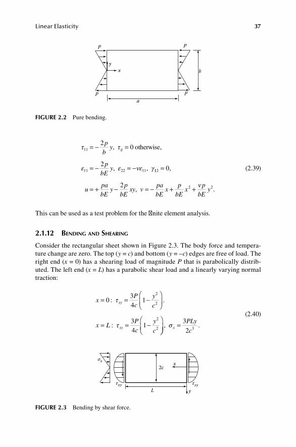
Linear Elasticity 37
τ τ
ε ε νε γ
11
11 22 11
20
2
= − =
= − = −
pb
y
pbE
y
ij, ,
, ,
otherwise
112
2 2
0
2
=
= + − = − + +
,
, .upabE
yp
bExy v
pabE
xp
bEx
pbE
yν
(2.39)
This can be used as a test problem for the finite element analysis.
2.1.12 Bending and Shearing
Consider the rectangular sheet shown in Figure 2.3. The body force and tempera-ture change are zero. The top (y = c) and bottom (y = –c) edges are free of load. The right end (x = 0) has a shearing load of magnitude P that is parabolically distrib-uted. The left end (x = L) has a parabolic shear load and a linearly varying normal traction:
xPc
y
c
x LPc
y
c
xy
xy
= = −
= = −
034
1
34
1
2
2
2
2
: .
:
τ
τ
=, .σ x
PLy
c
3
2 3
(2.40)
b
p
pa
p
xy
p
fIgure 2.2 Pure bending.
L
2cσx
τxyτxy
x
y
fIgure 2.3 Bending by shear force.

38 The Finite Element Method for Mechanics of Solids with ANSYS Applications
An exact solution is readily found by expressing u and v as polynomials in x and y. For plane stress,
σ
σ
τ
x
y
xy
Pxy
c
Pc
y
c
=
=
= −
3
2
0
34
1
3
2
2
,
,
,
(2.41)
and
uPx y
c E
Py
c E
Py
c G
Pyc
c Gey g
v
= + − + + +
= −
3
4 4 4
3
8
2
3
3
3
3
3
2
3
ν,
νν3
4 4
3
8
2
3
3
3
2
3
Pxy
c E
Px
c E
Pxc
c Gex h− + − + .
(2.42)
The constants e, g, and h represent rigid translation and rotation, and have to be determined from appropriate support conditions. For the case u(L,0) = 0, v(L,0) = 0, u(L,±c) = 0,
g
hPL
c E
c
L
ePL
c E
Pc
=
= − + +
= − −
0
21
4 52
3
4
3
3
2
2
2
3
,
,ν
ν 22
34 8c E
PcG
− .
(2.43)
The displacement at the origin is then
vPL
c E
c
L( , ) .0 0
21
4 52
3
3
2
2= − + +
ν
(2.44)
The first term is the displacement according to the elementary beam theory and the second is the additional displacement due to the shear that is neglected in the beam theory. For plane strain, replace ν by ν/(1 – ν) and E by E/(1 – ν2).
2.1.13 propertieS of SolutionS
Let us consider an equilibrium problem in the theory of elasticity for an isotro-pic material. The problem consists of determining the displacements, strains, and stresses that satisfy the partial differential equations of equilibrium,

Linear Elasticity 39
∂∂
τ ij
jix
b+ = 0,
(2.45)
the constitutive relations,
τkm = 2μεkm + λεiiδkm, (2.46)
the geometric equations,
ε km
k
m
m
k
ux
ux
= +
12
∂∂
∂∂
,
(2.47)
the boundary conditions on load,
τ ij j i Tn T= o on S ,
(2.48)
and the support conditions,
u ui i u= o on S . (2.49)
For plane stress or plane strain, there are corresponding equations in two dimensions.
Roughly speaking, a unique solution exists if the boundary of the body is smooth, the loads and support conditions are smooth, the support conditions prohibit rigid body displacements, and the material properties are smoothly distributed. The dis-placements, strains, and stresses are then continuous and finite throughout the body. However, problems for which there is a discontinuity in boundary, load, or support conditions are common. In such cases, the solution may have discontinuities or singularities.
One example of an isolated singularity is the apparently simple concept of a con-centrated force. A concentrated force F applied at a point x0 on the external surface is mathematically characterized by the requirements:
T FdA =∫∫S
(2.50)
for all parts S of the surface that contain x0, and
T u x F u x⋅ = ⋅∫∫ ( ) )d (A 0
S
(2.51)
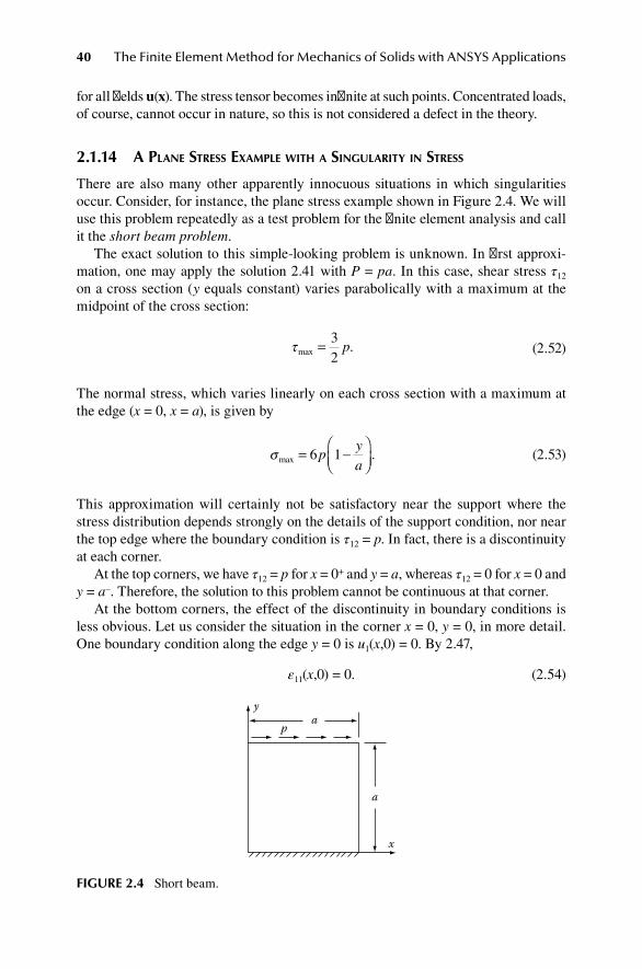
40 The Finite Element Method for Mechanics of Solids with ANSYS Applications
for all fields u(x). The stress tensor becomes infinite at such points. Concentrated loads, of course, cannot occur in nature, so this is not considered a defect in the theory.
2.1.14 a plane StreSS exaMple with a Singularity in StreSS
There are also many other apparently innocuous situations in which singularities occur. Consider, for instance, the plane stress example shown in Figure 2.4. We will use this problem repeatedly as a test problem for the finite element analysis and call it the short beam problem.
The exact solution to this simple-looking problem is unknown. In first approxi-mation, one may apply the solution 2.41 with P = pa. In this case, shear stress τ12 on a cross section (y equals constant) varies parabolically with a maximum at the midpoint of the cross section:
τ max = 3
2p.
(2.52)
The normal stress, which varies linearly on each cross section with a maximum at the edge (x = 0, x = a), is given by
σ max = −
6 1pya
.
(2.53)
This approximation will certainly not be satisfactory near the support where the stress distribution depends strongly on the details of the support condition, nor near the top edge where the boundary condition is τ12 = p. In fact, there is a discontinuity at each corner.
At the top corners, we have τ12 = p for x = 0+ and y = a, whereas τ12 = 0 for x = 0 and y = a–. Therefore, the solution to this problem cannot be continuous at that corner.
At the bottom corners, the effect of the discontinuity in boundary conditions is less obvious. Let us consider the situation in the corner x = 0, y = 0, in more detail. One boundary condition along the edge y = 0 is u1(x,0) = 0. By 2.47,
ε11(x,0) = 0. (2.54)
x
a
ap
y
fIgure 2.4 Short beam.

Linear Elasticity 41
On the other hand, one boundary condition along the edge x = 0 is τ11 = 0. From stress strain relation 2.46, we find that
ε ν
τ11
220 0( , )yE
= − ≠ .
(2.55)
From 2.54 and 2.55, we find the contradictory statements
ε
ε
11
11
0 0 0 0 0
0 0 0 0
( , ) ,
( , )
= → =
≠ →
for along
along
x y
y xfor == 0.
(2.56)
The mathematical consequence of this contradictory requirement is a singularity (infinite stress) at the corners where the free and fixed boundaries join.
The details of such a singularity are revealed by the solution of the problem for the infinite quarter plane (x ≥ 0, y ≥ 0) with zero displacements along the edge y = 0 and zero tractions along the edge x = 0. Using polar coordinates (r,θ), a solution has been found to be as follows2:
Eu r A B
k
kθ ν α αθ αβ
ν ν
= + +
+ + − −
+1 1
1 2 1
[( ) ( cos sin )
( ( ) ( ))(CC k D k
Eu r A Brk
cos sin )].
[( ) ( sin cos )
θ θ
ν α αθ αβ
+
= + −+1 1
++ + + −( ( ) )( sin cos )].k C k D k1 4ν θ θ
(2.57)
σ α α αθ αθ
α θ
rkr A B
k C k D k
= − +
+ − +
[( )( cos sin )
( )( cos sin
2
2 θθ
σ α α αθ αθ
θ θ
τ
θ
)] .
( )( cos sin
cos sin ).
= − +
+ +
r A B
C k D k
k 2
rrkr A B
k C k D k
θ α α αθ αθ
θ θ
= − −
+ −
( )[ ( sin cos )
( sin cos )].
1
(2.58)
The constant α = k + 2. The constants A, B, C, and D are determined by the four boundary conditions on the edges θ = 0 and θ = π/2. The solution depends on the Poisson ratio. For ν = 0.32, one finds a particular solution with k = –1/4. The displace-ments are finite at the corner (r = 0) but the stress components are infinite because of the negative exponent of r.
42 The Finite Element Method for Mechanics of Solids with ANSYS Applications
The numerical solutions that we will accomplish by the finite element method are approximations of the true solution to the field equations. The infinite stresses at a point are of course never found by numerical analysis, which deals only with finite real numbers. For each finer element mesh, one simply finds higher and higher stresses near the corners.
Another common situation where singularities occur is in the analysis of cracks that are modeled as a line or surface across which there is no contact force transmit-ted. In such problems, there is a singularity at the crack tip. A numerical method that introduces only continuous displacement fields cannot reproduce the exact solution. It is, however, possible to introduce special elements with built-in singularities in order to incorporate the crack tip singularities into the finite element model. This matter will be discussed later.
2.2 potentIal energy
Instead of seeking for the solution of the elasticity problem by solving the differential equations, we can seek those functions that make an appropriate operator stationary. First, let us consider the potential energy defined by
P A= − −∫ ∫[ ( ) ] ,εε b u V T u Ak k k k
T
d dV S
0
(2.59)
where ST is the part of the boundary on which the traction vector has the given value Tk
0. The strain tensor is defined by the kinematical relations 2.1, which is repeated here:
εkm = u(k,m). (2.60)
The stress tensor is regarded as defined by 2.8, which is repeated here:
τ
εkmkm
= ∂∂
A.
(2.61)
The potential energy is defined for all continuous functions uk with piecewise contin-uous first derivatives and which satisfy the boundary conditions on displacement:
u uk k u= o on S . (2.62)
For each set of functions uk, the integrals over the given region can be evaluated for a given material and a numerical value for P obtained. Imagine that this is done for all possible admissible functions and the values of P so obtained are compared. One would find that the true solution is the one that gives P a minimum value.

Linear Elasticity 43
To prove this assertion, suppose that vector u denotes the displacement vector for which P is a minimum. A necessary condition that P is a minimum is that the derivative of P is zero at point u. This condition is equivalent to the requirement that, for all vectors u,
∂ +∂
==
P( ).
u uαα
α 0
0
(2.63)
In carrying out this calculation for P defined by 2.59, note that
A A( ) ( ),u u+ = +α αεε εε (2.64)
where
εkm k mu= ( , ).
(2.65)
Therefore,
∂ +∂
= ∂∂=
A( ).
εε εεαα ε
εα 0
A
kmkm
(2.66)
Then, one obtains from 2.63 the following condition
{ } .( , )τ km k m k k k ku b u V T u A
TV S∫ ∫− − =d d0 0
(2.67)
Note that 2.67 is identical to the virtual work expression for the compatible system (ui ij, ε ) and ui = 0 on Su. Upon integrating the first term by parts, one finds
− + + − =∫ ∫( ) ( ) .,τ τkm m k k km m k kb u V n T u A
T
d dV S
0 0
(2.68)
Since this relation must hold for arbitrarily selected values of u, each of the expres-sions in parentheses must be zero in the indicated region. Thus, the condition that the first derivative of P is a zero at u, together with 2.2 and 2.3, is equivalent to the requirement that the differential equations and boundary conditions 2.45 to 2.49 are satisfied.
The procedure used in this section is called the “calculus of variations” in the older literature. It developed before the modern concepts of abstract operator and

44 The Finite Element Method for Mechanics of Solids with ANSYS Applications
abstract derivative. Calculation of the functional derivation of P is equivalent to cal-culation of “the first variation of P.”
We have not shown that P is a minimum at the true solution. The preceding calculations only show that the first derivative is zero at the true solution and vice versa. This is a necessary condition for a minimum, but it is not sufficient. Thus far, one can only say that the potential energy is stationary at the true solu-tion, and it might be a maximum or a minimum or something like a point of inflection.
2.2.1 proof of MiniMuM potential energy
We will now prove that the potential energy is indeed a minimum at the true solution in the case of isothermal deformations. The proof hinges on the following property of the strain energy A. It is easy to see for the isotropic material that A(ε) is non-negative for every tensor ε since it is the sum of squares of the components of ε. It is zero only when all components of the strain tensor are zero. We assume that the strain energy always has this property.
Let ui* be any set of smooth functions that satisfy the displacement boundary
conditions:
u ui i u* .= o on S (2.69)
Let εij* be the set of functions derived from ui
* by the strain–displacement equations:
εij i ju* * .( , )=
(2.70)
Let τ ij* be the set of functions derived from εij
* by the constitutive relations:
τ εij ijkm kmc* * .=
(2.71)
These stresses need not satisfy the equilibrium equations or the boundary conditions on load. If those relations are satisfied, then the system (u*, ε*, τ*) is the actual solu-tion. We wish to consider the case when it is not the true solution.
Suppose the actual solution to the given boundary value problem is denoted by u, ε, τ. We first note that
τ ε ε ε ε ε τ εij ij ijkm km ij kmij km ij km kmc c* * * *= = =
(2.72)
because of the symmetry of cijkm. Now, consider the expression

Linear Elasticity 45
12
12
( * )( * ) ( * )( *τ τ ε ε ε ε ε εij ij ij ij ijkm ij ij kmc− − = − − kkm ) ( * )= − >A εε εε 0.
(2.73)
Using relations 2.72 and 2.73, it follows that
2( * ) * * *( * )τ τ ε τ ε τ ε τ ε ε εij ij ij ij ij ij ij ij ij ij− = − − − − iij ij ij
ij ij ij ij ij ij ij
( *)
* * ( * )( *
τ τ
τ ε τ ε τ τ ε ε
−
= − − − − iij
ij ij ij ij
)
* * .< −τ ε τ ε
(2.74)
Consequently, using 2.72,
12
( * * ) ( * ).τ ε τ ε τ ε εij ij ij ij km km km− > −
(2.75)
By the virtual work formula,
( * ) ( * ) ( * )ε ε τij ij ij i i i
S
i i i
V
V u u T A u u b V− = − + −∫ ∫d d d
F
0 ∫∫ ,
(2.76)
since u u ui i i= =* 0 on Su. Integrating expression 2.75 over the body, using 2.76, and rearranging the terms, we find
12
12
0τ ε τ εij ij
V
i i
S
i i
V
ij ijV u T A u b V V* * * *d d d d
F
∫ ∫ ∫− − > ∫∫ ∫ ∫− −u T A u b Vi i
S
i i
V
0 d d
F
.
(2.77)
Thus, the potential energy of any compatible system is greater than the potential energy of the actual solution:
P(u*) > P(u). (2.78)
That is, the potential energy is a minimum for the actual solution. Among all the displacement fields that satisfy the support conditions, the solution for the given load condition is the displacement field that makes the potential energy a minimum.
2.3 MatrIx notatIon
We will often use matrix notation instead of the component notation. Each notation has certain advantages. In matrix notation, the components of the stress and strain tensors will be arranged in a column matrix. For the plane problems,
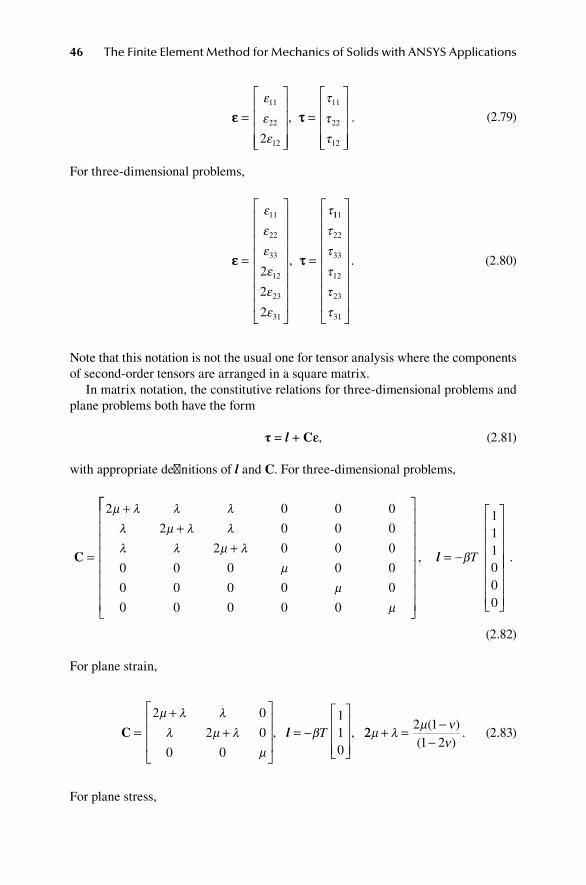
46 The Finite Element Method for Mechanics of Solids with ANSYS Applications
εε ττ=
=
ε
ε
ε
τ
τ
τ
11
22
12
11
22
122
,
.
(2.79)
For three-dimensional problems,
εε ττ=
=
ε
ε
ε
ε
ε
ε
τ11
22
33
12
23
31
2
2
2
,
111
22
33
12
23
31
τ
τ
τ
τ
τ
.
(2.80)
Note that this notation is not the usual one for tensor analysis where the components of second-order tensors are arranged in a square matrix.
In matrix notation, the constitutive relations for three-dimensional problems and plane problems both have the form
τ = l + Cε, (2.81)
with appropriate definitions of l and C. For three-dimensional problems,
C =
++
+
2 0 0 0
2 0 0 0
2 0 0 0
0 0 0 0 0
0 0 0 0 0
0 0 0 0 0
µ λ λ λλ µ λ λλ λ µ λ
µµ
µ
= −
, l βT
111000
.
(2.82)
For plane strain,
C =+
+
= −
2 0
2 0
0 0
110
µ λ λλ µ λ
µβ, ,l T 22
2 11 2
µ λµ ν
ν+ = −
−( )
( ).
(2.83)
For plane stress,

Linear Elasticity 47
C =− −
= − −−
ET
1
1 01 0
0 01
2
1 21
110
2ν
νν
νβ
νν
, l
.
(2.84)
In practical applications, materials are usually orthotropic at most and data are usu-ally stated for the inverse of C:ε = C–1τ. For orthotropic materials, C–1 has the form:
C− =
− −
− −
− −1
10 0 0
10 0 0
E E E
E E E
E
x
xy
y
xz
z
yx
x y
yz
z
zx
x
ν ν
ν ν
ν νν zy
y z
xy
yz
xz
E E
G
G
G
10 0 0
0 0 01
0 0
0 0 0 01
0
0 0 0 0 01
=
,
ν νxy
y
yx
xE E
νν ν
ν ν
xz
z
zx
x
yz
z
zy
y
E E
E E
=
=
.
(2.85)
The components of the vectors Ti, bi, and ui are arranged in column matrices in the usual manner: the index indicates the row number. The virtual work formula then takes the form:
u T u bT T Td d dA V VS V V∫ ∫ ∫+ = εε ττ .
(2.86)
For isothermal deformations, the strain energy becomes
A( ) .εε ττ εε= = =1
212
12
cijkm ij km ij ijε ε τ ε T
(2.87)
The potential energy then becomes
PV S
= −
−∫ ∫1
2d dT T Tττ εε b u V A
T
( ) .T u0
(2.88)
The form for plane problems is analogous.
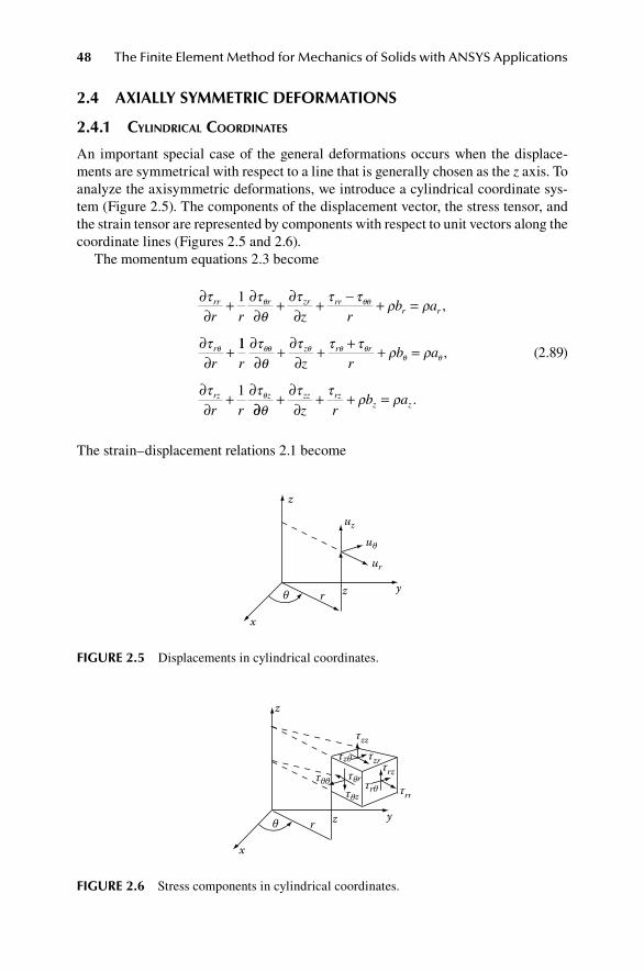
48 The Finite Element Method for Mechanics of Solids with ANSYS Applications
2.4 axIally SyMMetrIc deforMatIonS
2.4.1 cylindrical coordinateS
An important special case of the general deformations occurs when the displace-ments are symmetrical with respect to a line that is generally chosen as the z axis. To analyze the axisymmetric deformations, we introduce a cylindrical coordinate sys-tem (Figure 2.5). The components of the displacement vector, the stress tensor, and the strain tensor are represented by components with respect to unit vectors along the coordinate lines (Figures 2.5 and 2.6).
The momentum equations 2.3 become
∂∂
+ ∂∂
+ ∂∂
+ − + =
∂∂
+
τ τθ
τ τ τρ ρ
τ
θ θθ
θ
rr r zr rrr r
r
r r z rb a
r
1,
11
1
r z rb a
r r
z r r
rz z
∂∂
+ ∂∂
+ + + =
∂∂
+ ∂
τθ
τ τ τρ ρ
τ τ
θθ θ θ θθ θ
θ
,
∂∂+ ∂
∂+ + =
θτ τ
ρ ρzz rzz zz r
b a .
(2.89)
The strain–displacement relations 2.1 become
z
uz
ur
uθ
θ zr
x
y
fIgure 2.5 Displacements in cylindrical coordinates.
z
τzz
τθθτθz
τzθτθr τrθ
τzr
τrr
τrz
yzr
x
θ
fIgure 2.6 Stress components in cylindrical coordinates.
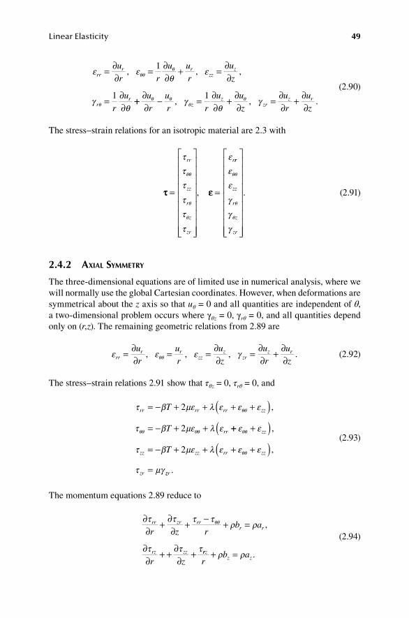
Linear Elasticity 49
ε εθ
ε
γθ
θθθ
θ
rrr r
zzz
rr
ur r
u ur
u
z
ru
= ∂∂
= ∂∂
+ = ∂∂
= ∂∂
, , ,1
1 ++ ∂∂
− = ∂∂
+ ∂∂
= ∂∂
+ ∂∂
ur
ur r
u uz
u
ruzz
zzr
z rθ θθ
θγθ
γ, , .1
(2.90)
The stress–strain relations for an isotropic material are 2.3 with
ττ εε=
=
τ
τ
τ
τ
τ
τ
ε
θθ
θ
θ
rr
zz
r
z
zr
r
,
rr
zz
r
z
zr
ε
ε
γ
γ
γ
θθ
θ
θ
.
(2.91)
2.4.2 axial SyMMetry
The three-dimensional equations are of limited use in numerical analysis, where we will normally use the global Cartesian coordinates. However, when deformations are symmetrical about the z axis so that uθ = 0 and all quantities are independent of θ, a two-dimensional problem occurs where γθz = 0, γrθ = 0, and all quantities depend only on (r,z). The remaining geometric relations from 2.89 are
ε ε ε γθθrr
r rzz
zzr
z rur
ur
u
z
u
ruz
= ∂∂
= = ∂∂
= ∂∂
+ ∂∂
, , , .
(2.92)
The stress–strain relations 2.91 show that τθz = 0, τrθ = 0, and
τ β µε λ ε ε ε
τ β µε λ ε
θθ
θθ θθ
rr rr rr zz
rr
T
T
= − + + + +( )= − + +
2
2
,
++ +( )= − + + + +( )=
ε ε
τ β µε λ ε ε ε
τ µγ
θθ
θθ
zz
zz zz rr zz
zr
T
,
,2
zzr .
(2.93)
The momentum equations 2.89 reduce to
∂∂
+ ∂∂
+ − + =
∂∂
+ + ∂∂
+
τ τ τ τρ ρ
τ τ τ
θθrr zr rrr r
rz zz
r z rb a
r z
,
rrzz zr
b a+ =ρ ρ .
(2.94)

50 The Finite Element Method for Mechanics of Solids with ANSYS Applications
The axisymmetric equations are usually applied to a circular cylinder with the gen-erator along the z axis and surface loads and supports symmetrical about the z axis.
2.4.3 plane StreSS and plane Strain
The cylindrical coordinates are often useful for the analytical formulation and solu-tion of plane problems where the region is a cross section of a circular cylinder. In this case, τzr = 0, τzθ = 0, and all quantities depend only on (r,θ). The balance of momentum 2.89 gives
∂∂
+ ∂∂
+ − + =
∂∂
+ ∂∂
τ τθ
τ τρ ρ
τ τ
θ θθ
θ θθ
rr r rrr r
r
r r rb a
r r
1
1
,
θθτ τ
ρ ρθ θθ θ+ + + =r r
rb a .
(2.95)
The geometric relations 2.90 give
ε ε
θγ
θθθθ
θθ θ
rrr r
rru
r ru u
r ru u
rur
= ∂∂
= ∂∂
+ = ∂∂
+ ∂∂
−, ,1 1
..
(2.96)
The stress–strain relations for an isotropic material are 2.83 and 2.84 with
ττ εε=
=
τ
τ
τ
ε
ε
γθθ
θ
θθ
θ
rr
r
rr
r
, ..
(2.97)
2.5 proBleMS
1. For an isotropic material, prove that s e T Bkm km kk kk= = − +µ τ β ε213
and .
2. For an isotropic material, prove that εν
τν
τ δ α δkm km ii km kmE ET= + − +1
.
3. Determine the substitution for ν that transforms the plane stress equations into plane strain equations.
4. For an isotropic material, (a) calculate the components of the strain tensor and the stress tensor for the following set of given displacements for an isotropic material:
u
Ex u
Ex u
Ex1 1 2 2 3 3= = − = −σ
νσ
νσ
, , ,

Linear Elasticity 51
where σ is a constant. (b) Check the equilibrium equations to see if they are satisfied for zero body forces. (c) Show the edge tractions on a diagram of the body 0 ≤ x1 ≤ L, 0 ≤ x2 ≤ a, 0 ≤ x3 ≤ b.
5. A rectangular sheet of unit thickness is loaded by uniform shear stress along each edge (see Figure 2.1). If the origin has zero displacement and the dis-placement v = 0 at point (a, 0), the proposed solution is given by 2.38. Check the equations of linear elasticity for an isotropic material to see if this pro-posed solution is correct for zero body forces and zero acceleration.
6. Consider the plane stress problem diagrammed in Figure 2.2. The origin has zero displacement and v = 0 at point (a,0). Check the proposed solution 2.39 for zero body force and zero inertial force.
7. The plane stress problem of Figure 2.4 is to be analyzed using only the left half (0 ≤ x ≥ a/2) and symmetry/antisymmetry. Determine the boundary conditions to be applied to the line x = a/2.
8. The plane stress problem in Figure 2.3 is to be analyzed using only the upper half (0 ≤ y ≥ c) and symmetry/antisymmetry. Determine the boundary conditions to be applied to line y = 0.
9. The plane stress problem of stretching of a sheet with a hole shown in Figure 2.7 is to be solved using only the upper right quarter. Determine the boundary conditions to be applied to the lines x = 0 and y = 0.
10. A solid cylinder of radius R and length L is loaded by a uniformly distrib-uted tensile load on each end: τzz = σ for z = 0 and z = L. Assume for a trial solution that the deformations are axisymmetric and uz = c1z and ur = c2r, where c1 and c2 are constants. Show that the elasticity equations and bound-ary conditions on load can be satisfied and determine the required values of constants c1 and c2.
referenceS
1. Sololnikoff, I. S., Mathematical Theory of Elasticity, McGraw-Hill, New York, 1956, 67. 2. Williams, M. L., Stress singularities resulting from various boundary conditions in
angular corners of plates in extension, J. Appl. Mech. 19, 526, 1952.
S S2b
y
ax
fIgure 2.7 Sheet with a hole.

52 The Finite Element Method for Mechanics of Solids with ANSYS Applications
BIBlIography
Dill, E. H., Continuum Mechanics: Elasticity, Plasticity, Viscoelasticity, CRC Press, Boca Raton, FL, 2007.
Malvern, L. E., Introduction to the Mechanics of Continuous Media, Prentice-Hall, Englewood Cliffs, NJ, 1969.
Sololnikoff, I. S., Mathematical Theory of Elasticity, McGraw-Hill, New York, 1956.Timoshenko, S., and J. N. Goodier, Theory of Elasticity, McGraw-Hill, New York, 1951.Washizu, K., Variational methods in elasticity and plasticity, 2nd ed., Pergamon Press, New
York, 1974.
53
3 Finite Element Method for Linear Elasticity
A linear elastic analysis is the basis of most engineering designs. However, exact solutions to the differential equations of linear elasticity are known for only the sim-plest loadings on the simplest configurations. One needs a way to construct solutions for any configuration and all load and support conditions. The finite element method is well suited for this purpose. We are concerned with a procedure for obtaining an accurate numerical solution to the exact equations.
However, the engineer should not forget that the theory of linear elasticity is an imperfect model of material behavior. Its usefulness in engineering design is limited by the simplicity of the model, and because the exact mathematical solutions of boundary value problems are sometimes physically unrealistic. Consequently, the effort to obtain extremely accurate numerical solutions may not be worthwhile in some cases. The limits on applicability of the model to the physical situation must be kept in mind when the solution of the elasticity problem is used in an engineering application.
The finite element method was developed in detail in Chapter 1 for naturally artic-ulated structures. We now investigate the method for two- and three-dimensional solids. The fundamental idea is to divide the body into small pieces that we call ele-ments. The displacement field is then approximated in each element by interpolating between the values of the displacement at specific points on the element that we call nodes. The displacement field generated in this manner is substituted into the expres-sion for the potential energy, which then depends only on the nodal displacements. The condition that P is a minimum generates a set of linear algebraic equations for the nodal displacements.
In the derivation of the theorem of minimum potential energy in Chapter 2, we assumed that the displacement field is continuous. We should therefore choose the expressions for the displacements within an element in such a way that the global displacement field is continuous for any and all nodal displacements. If this is done, the elements are said to be conforming. Nonconforming elements may be satisfac-tory in certain cases, which we will discuss later.
We number the elements consecutively from 1, 2, 3, …, M and also number the components of unknown nodal displacement throughout the body consecutively from 1, 2, 3, …, N. For three dimensions, N is three times the number of nodes. For plane stress or plane strain, N is two times the number of nodes.
In the following discussion of the finite element method, we will assume that the boundary of the body coincides with the boundary of the finite element model. This eliminates the geometric error resulting from the approximation for curved bound-aries by polygonal elements. In practical applications, that is often not the case and

54 The Finite Element Method for Mechanics of Solids with ANSYS Applications
there will be a geometric error; but, of course, we suppose that error tends to zero as the size of the elements tends to zero.
3.1 fInIte eleMent approxIMatIon
Let us consider one particular element and one component ui of displacement within that element. The component ui will depend on the nodal displacements DK for that element, but only on the displacements at nodes falling within that element or on its boundary, and not on the displacement of a node that does not fall within that ele-ment. We will only use an interpolation process for which the relation is linear:
u N Di iK K
K m
( ) ( ) ,x x=∈
∑I
(3.1)
where Im is the set of nodal displacements for the mth element. In this chapter, we will apply the summation convention only to the lower-case indices. The index i has the range (1, 2) for the plane problem and the range (1, 2, 3) for the three-dimensional problem. The interpolation functions NiK are called shape functions for the element. Different shape functions could be used for each element but we will usually use the same ones for all elements. Furthermore, each component of displacement will depend only on the nodal values of that same component.
The shape functions must be such that a continuous displacement field is gener-ated that is capable of approximating the true solution with an error that tends to zero as the size of each element tends to zero. In particular, we must have the following conditions:
(1) Continuity along element boundaries for arbitrary nodal displacements. (2) Shape functions must be able to exactly represent a state of constant strain. (3) If ui(xJ) = DM, then
N D DiK J K
K
M
m
( )x∈
∑ =I
.
(3.2)
The second condition will be satisfied if a polynomial is used that contains the con-stant and linear terms. We will consider the choice of shape functions in more detail in subsequent chapters.
Given the shape functions, the strains are calculated by Equation 2.1:
εij ijK K
K
A D
m
=∈
∑I
,
(3.3)
where
ANx
N
xijKiK
j
jK
i
= +
12
∂∂
∂∂
.
(3.4)

Finite Element Method for Linear Elasticity 55
The stress, calculated by 2.11, has the form
τ ij ij ijK K
K
l B D
m
= +∈
∑I
,
(3.5)
where
BijK = cijkmAkmK. (3.6)
The values of cijkm and lij depend on whether the problem is plane stress or plane strain or three dimensional. From 2.9, for each element
A
I
( )εε = +
=∈∈
∑
12
12
c l
A B D D
ijkm ij km ij ij
ijK ijM K M
MK m
ε ε ε
II Im m
l A Dij
K
ijK K∑ ∑+∈
.
(3.7)
Indices K and M range over the index set for the particular element.
3.1.1 potential energy
The elements partition the region V into subregions Vm. Let Sm denote the part, if any, of the boundary of the subregion Vm that lies on the exterior surface. We will ini-tially regard the entire exterior surface as having specified loads. Then, the potential energy 2.59 is the sum of the potential energy of each element:
P P==
∑ m
m
M
1
,
(3.8)
and
P AV S
m i i i ib u V T u A
m m
= − −∫ ∫[ ( ) ] .εε d do
(3.9)
For plane stress or plane strain, the volume integrals reduce to integrals over the two-dimensional region of the element and the bounding surface of the body is a curve. Next, substitute expression 3.1 for the displacement field of an element, and expression 3.7 for the strain energy, into expression 3.9 for the potential energy of the element. This gives
P
I I
m
I J
IJm
I J Im
I
I
m m
k D D f D= −∈ ∈
∑ ∑12
,
,
(3.10)

56 The Finite Element Method for Mechanics of Solids with ANSYS Applications
where
k B A VIJm
kiI kiJ
m
= ∫ dV
,
(3.11)
f l A V b N V T N AIm
ki kiI k kI k kI
m m m
= − + +∫ ∫ ∫d d do
V V S
.
(3.12)
Expression 3.8 for the total potential energy of the body is now a summation of the corresponding terms in 3.10. All of the coefficients of a particular pair, DI,DJ, I,J = 1 to N, are added together. If a pair does not appear in 3.10, the coefficient is zero. Thus,
P = −== =
∑∑ ∑12
11 1
K D D F DIJ I J
J
N
I
N
J J
J
N
,
(3.13)
where
K kIJ IJm
m
M
==
∑1
,
(3.14)
F fI Im
m
M
==
∑1
.
(3.15)
For three dimensions, the range N of (I,J) is from one to three times the number of nodes. For the plane problem, the sum is twice the number of nodes. The matrix of elements KIJ is called the global stiffness matrix. The matrix with elements FI is called the global force matrix. The matrix K has N rows and columns. The matrix F has N rows. The total number of displacement components N is called the degree of freedom of the unsupported body.
The summation in 3.14 and 3.15 is in the sense of a merge of the element matrices as detailed in Chapter 1. Since the range of I and J in 3.10 depends on the element m, we can view the merge in two ways.
First, in order to carry out the sum on m, we can extend the summation in 3.10 to all displacement parameters by defining kIJ
m to be zero for all I and J that are not in the set Im. Then the merge of element matrices is a simple addition of all element matrices with like indices. This is the method of augmented matrices detailed in Chapter 1. Alternatively, we can set KIJ = 0 initially, and then, for each element, we add kIJ
m to the KIJ term with matching indices. This is the process of direct merge of the element matrices.

Finite Element Method for Linear Elasticity 57
The stiffness matrix for the unsupported structure has a zero determinant since the displacements can be determined only to within a rigid translation and rotation.
The components of the force matrix satisfy the identity
F D T u A b u V l VJ J i i
J
i i ij ij≡ + −∫∑ ∫ ∫d d dS V V
ε .
(3.16)
That is, each FI is energy equivalent to a concentrated force corresponding to the displacement component DI. Loads satisfying 3.16 are called consistent with the energy formulation.
3.1.2 finite eleMent equationS
Expression 3.13 for the potential energy is now a quadratic algebraic form with vari-ables DI. The condition that P be a minimum is
∂ =P∂DI
0.
(3.17)
Applying this condition yields a set of N linear algebraic equations in N unknowns:
K D FIJ J
J
N
I
=∑ =
1
.
(3.18)
These equations must be solved numerically for the unknown nodal displacements DJ. The displacement, strain, and stress fields for an element can then be calculated from 3.1 to 3.5.
Since we have supposed the entire exterior surface to have specified loads and no specified displacements, the body can experience rigid translations and rotations. The solution to 3.18 for the unsupported structure is therefore not unique (in the absence of inertial forces). In fact, the determinant of K will be zero.
If, instead, the displacement is given over a part Su of the boundary, the func-tions ui must satisfy those displacement boundary conditions. Therefore, the nodal displacements DI must have values that make ui satisfy the conditions on Su, at least approximately. If a node falls on a portion of the boundary, the value of a component of nodal displacement is known, and the corresponding component of nodal force is an unknown reaction. We apply a displacement boundary condition by substitut-ing the given value of DI in 3.18 and use the corresponding Ith equation to evaluate the reaction FI. Therefore, if there are any displacement boundary conditions, the number N of unknown degrees of freedom of the supported body will be less than three times the number of nodes and the number of equations is similarly reduced. If the specified displacements are sufficient to prevent rigid translation and rotation, the determinate of K will be nonzero, and a unique solution to 3.18 will exist for the unspecified nodal displacements.
58 The Finite Element Method for Mechanics of Solids with ANSYS Applications
3.1.3 BaSic equationS in Matrix notation
The preceding relations can be written more concisely if the various arrays are arranged into matrices. Let us put the displacement components ui in a column matrix u. There will be three rows for the three-dimensional bodies and two rows for the 2D problems. Let us also put the parameters DK in a column matrix D. Then Equation 3.1, which applies to each element, becomes
u = ND (3.19)
where the shape functions NiK are arranged in a rectangular matrix. The number of rows in matrix D is equal to the number of displacement parameters for the element. If we use the scheme in 2.79 or 2.80 to arrange the components of the strain tensor in a column matrix, then Equation 3.3 becomes
ε = AD (3.20)
where functions AijK have been arranged in a rectangular matrix. The constitutive relations have the form 2.81, which is repeated here:
τ = l + Cε. (3.21)
Equation 3.5 then becomes
τ = l + BD (3.22)
where
B = CA, (3.23)
all expressed as rectangular matrices. The element stiffness matrices in 3.11 are rectangular matrices given by
k B Am V
m
= ∫ T d .V
(3.24)
The nodal forces contributed by the mth element (3.12) are given by
f N T N b Am
m m m
A V V= + −∫ ∫ ∫T T Td d d0
S V V
l .
(3.25)
The element matrices km and fm are merged to obtain the global stiffness matrix K and global force matrix F, and the final equations to be solved (3.18) can be writ-ten as
Finite Element Method for Linear Elasticity 59
KD = F. (3.26)
Matrix D now includes the full list of N unknown displacement parameters for the whole body, and force matrix F has an equal number of rows. The global stiffness matrix K is a symmetric and banded square matrix with N rows and N columns, where N is the number of unknown displacements.
3.1.4 BaSic equationS uSing Virtual work
Instead of using the theorem of minimum potential energy to establish the equilib-rium equations, one may use the virtual work theorem that is expressed in matrix form by 2.86. Applied to the assemble of finite elements, we have
u uT T Td d dT bA V V
mm
M
m
M
m
M
S V V∫∑ ∫∑ ∫∑
= = =
+ =1 1 1
m m
εε ττ .
(3.27)
Surface Sm is that part of the surface of element m that is a part of the exterior surface of the body (if any).
The shape functions 3.1 used to approximate the actual displacements can also be used to generate a compatible displacement field:
u ND= , (3.28)
where D is the column matrix of nodal displacements of the compatible system, the so-called virtual displacements. Virtual displacements are numbered in the same manner as the actual nodal displacement. The compatible strains are then deter-mined by the strain–displacement equations as in 3.3:
εε = AD. (3.29)
That is, the same coefficient matrix A occurs. Substituting 3.28 and 3.29 into 3.27, and merging the element matrices, we have
D N T N b D AT T T T Td d dA V V
mm
M
m
M
S V V∫∑ ∫∑
= =
+
=1 1
m m
ττ∫∫∑=
m
M
1
.
(3.30)
Since this relation must hold for every compatible system, it must hold for arbitrary D. Therefore, a necessary condition for equilibrium of the finite element approxima-tion of the stress state is
N T N b AT T Td d dA V V
m m mm
M
m
M
m
M
S V V∫∑ ∫∑ ∫∑
= = =
+ =1 1 1
ττ .
(3.31)

60 The Finite Element Method for Mechanics of Solids with ANSYS Applications
Note that this relation is true for any material body, whether elastic or not. It simply expresses the balance of the external applied nodal forces and the internal resisting nodal forces, F = f, where the external applied nodal forces are
F N T N b= +∫∑ ∫∑= =
T Td dA V
m mm
M
m
M
S V1 1
,
(3.32)
and the internal resisting nodal forces are
f A= ∫∑=
T dττ Vm
M
Vm
.1
(3.33)
This is the virtual work formula for the finite element approximation. Note that f here is not the same as fm in Equation 3.25. The summation is in the sense of merge of the element matrices. Substituting formula 3.22 for the stress in each element, we find
f A B D KD=
=∫∑=
T dVm
M
Vm1
(3.34)
for an elastic material. Therefore,
F = KD, (3.35)
where F is, again, given by merging the element force matrices 3.12 and K is deter-mined by merging the element stiffness matrices 3.11.
3.1.5 undereStiMate of diSplaceMentS
We will now show that the displacements calculated by the finite element approximation to the potential energy are always “smaller” than the actual displacements. In matrix notation, the finite element approximation 3.13 to the potential energy becomes
P* .= −1
2D KD D FT T
(3.36)
Since KD = F, it follows that, for the solution set, P* is given by
P* .= − 1
2F DT
(3.37)
Since the strains are derived from a continuous displacement field by the geomet-ric relations and the stresses are derived from that strain field by the constitutive
Finite Element Method for Linear Elasticity 61
equations, the finite element solution is an example of a compatible system provided that the displacement boundary conditions are exactly satisfied. The potential energy of such a compatible system is greater than the potential energy of the actual solu-tion, which is a minimum.
Suppose that there is no temperature change so that 2A = τijεij; then, using the virtual work formula 2.7, the potential energy (2.59) of the actual solution is
PS V S
( ) ,u = − −∫ ∫ ∫12
12
0T u A b u V T u Ai i i i i i
T
d d d
(3.38)
where S = ST + Su. If the displacement boundary conditions are ui = 0 on Su, then the potential energy of the actual solution becomes
PS V
( ) .u = − −∫ ∫12
12
0T u A b u Vi i i i
T
d d
(3.39)
Since the potential of the true solution is a minimum,
P* > P. (3.40)
Therefore, from 3.37 and 3.39,
F DT o d d< +∫ ∫T u A b u Vi i i i
TS V
.
(3.41)
That is, the work FTD of the nodal forces for the calculated displacements is less than the work of the given loads. A more precise result is obtained if the applied load is a single concentrated force. Suppose, for example, that the only load is a concentrated unit force in the x direction at the node n. Then, FI = 0 except for the x component at node n, which is equal to 1. Let Un denote the x displacement at node n, then 3.41 yields
Un < u1(Xn), (3.42)
where Xn is the position of node n, that is, the calculated nodal displacement is less than the actual displacement at that point.
3.1.6 nondiMenSional equationS
In the numerical examples, we will usually solve the equations using any conve-nient values for the dimensions, material properties, and loads. The solution for any other units can be deduced from the following nondimensional equations of elasticity.

62 The Finite Element Method for Mechanics of Solids with ANSYS Applications
Let p have the units of stress and a have the units of length. Define nondimen-sional coordinates, displacements, stress, and strain by
ˆ , ˆ , ˆ , ˆ , ˆ , ˆ ,xx
u u TT== ττ ττ εε εε ==
aEpa p
Ep p
tE
at= = = =0 0 0
2ρ
(3.43)
where a, p, and E0 are any convenient scale factors for the length scale, load mag-nitude, and material modulus, respectively. The new variables are then nondimen-sional. The basic equations of elasticity for zero body force and neglecting inertial forces are
∂∂
= ∂∂
= ∂∂
+∂∂
ˆ
ˆ
ˆˆ
ˆ,
ˆˆ
ˆ
ˆ
τ
ε
ij
j
i
iji
j
j
i
xu
t
ux
u
x
2
2
12
=+
++ −
,
( )( ),ˆ ˆ ˆ
ˆ
τν
ενν ν
ε δij ij kk ij
E E E E/ /0 0
1 1 1 2
ττ ij j in T= ˆ .
(3.44)
Note that the actual value of Poison’s ratio must be used since it cannot be factored out of the equations. In the finite element relations, define nondimensional quantities by
ˆ , ˆ , ˆ , ˆ , ˆ .D D A A K K C C F F= = = = =Epa
aaE E pa
0
0 02
1 1 1
(3.45)
The finite element relations are then
ˆ ˆ ,
ˆ ˆ ˆ,
ˆ ˆ ˆ ,
ˆ ˆ ˆ ˆ ˆ ,
ˆ ˆ ˆ .
u ND=
=
=
=
∫
ττ == εε
εε
C
AD
K A CA
KD F
T dVV
(3.46)
Having redefined the variables, we can then drop the ̂ in 3.46. We will use nondimen-sional quantities in most examples. A problem is solved for any convenient values of a, p, E0, and ρ. The actual stress and displacement can then be calculated using 3.43.
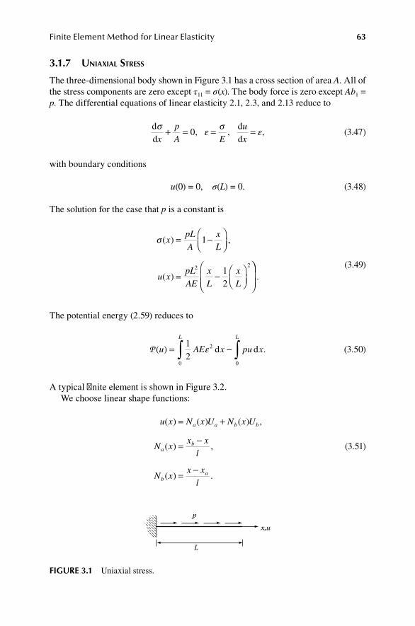
Finite Element Method for Linear Elasticity 63
3.1.7 uniaxial StreSS
The three-dimensional body shown in Figure 3.1 has a cross section of area A. All of the stress components are zero except τ11 = σ(x). The body force is zero except Ab1 = p. The differential equations of linear elasticity 2.1, 2.3, and 2.13 reduce to
dd
dd
σε
σε
xpA E
ux
+ = = =0, , ,
(3.47)
with boundary conditions
u(0) = 0, σ(L) = 0. (3.48)
The solution for the case that p is a constant is
σ ( ) ,
( )
xpLA
xL
u xpLAE
xL
xL
= −
= −
1
12
2 2
.
(3.49)
The potential energy (2.59) reduces to
P( ) .u AE x pu x
L L
= −∫ ∫12
2
0 0
ε d d
(3.50)
A typical finite element is shown in Figure 3.2.We choose linear shape functions:
u x N x U N x U
N xx x
l
N xx x
l
a a b b
ab
ba
( ) ( ) ( ) ,
( ) ,
( ) .
= +
= −
= −
(3.51)
x,u
p
L
fIgure 3.1 Uniaxial stress.
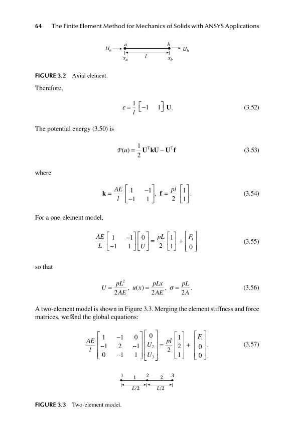
64 The Finite Element Method for Mechanics of Solids with ANSYS Applications
Therefore,
ε = −
11 1
lU.
(3.52)
The potential energy (3.50) is
P( )u = −1
2U kU U fT T
(3.53)
where
k f= −−
=
AE
l
pl1 11 1 2
11
, .
(3.54)
For a one-element model,
AEL U
pL F1 11 1
02
11 0
1−−
=
+
(3.55)
so that
U
pLAE
u xpLxAE
pLA
= = =2
2 2 2, ( ) , .σ
(3.56)
A two-element model is shown in Figure 3.3. Merging the element stiffness and force matrices, we find the global equations:
AEl
U
U
p1 1 01 2 1
0 1 1
0
2
122
3
−− −
−
= l
1100
1
+
F.
(3.57)
Ub
xblxa
Uaa b
fIgure 3.2 Axial element.
L/2
1
L/2
1 2 2 3
fIgure 3.3 Two-element model.

Finite Element Method for Linear Elasticity 65
Therefore,
U
pLAE
UpLAE2
2
3
238
12
= =, .
(3.58)
For element 1,
u x
xl
UEl
UplA
( ) , .= = =2 232
σ
(3.59)
For element 2,
u x
L xl
Ux l
lU
El
U UpL
A( )
( ) (, .= − + − = −( ) =2 3 3 2 4
)σ
(3.60)
The results are compared with the exact solution in Figures 3.4 and 3.5 for non-
dimensional variables 2
2
AE
pLu u
ApL
S→ →, σ . The displacement is uniformly too
small. The stress is too large at some points and too small at others. The energy measure 3.41 for the two-element model is as follows:
F DT =
=pLU
U
p LAE4
1 2 10
5162
3
2 3
.
(3.61)
1
0.9
0.8
0.7
0.6
0.5
0.4
0.3
0.2
0.1
00 0.5 1
xU one element
two elements
u
fIgure 3.4 Displacement.
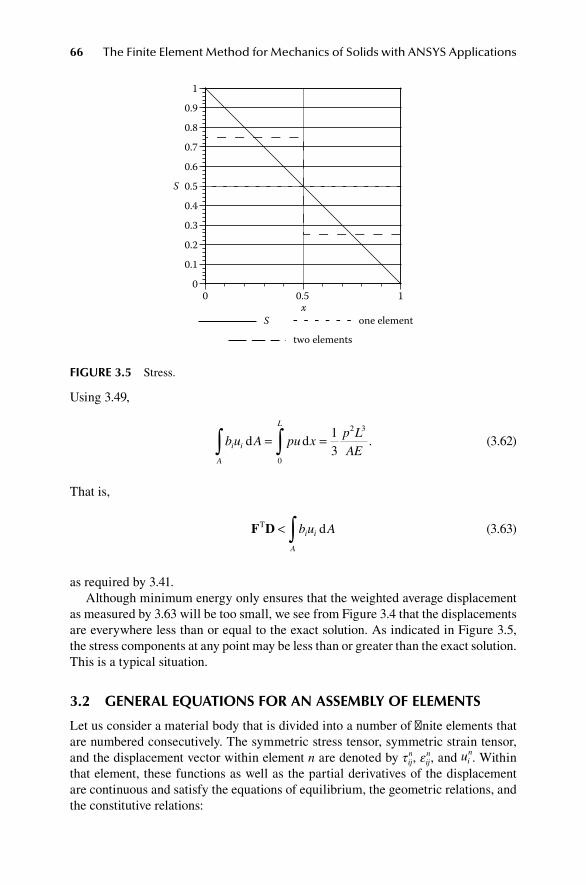
66 The Finite Element Method for Mechanics of Solids with ANSYS Applications
Using 3.49,
b u A pu xp LAEi i
A
L
d d∫ ∫= =0
2 313
.
(3.62)
That is,
F DT d< ∫ b u Ai i
A
(3.63)
as required by 3.41.Although minimum energy only ensures that the weighted average displacement
as measured by 3.63 will be too small, we see from Figure 3.4 that the displacements are everywhere less than or equal to the exact solution. As indicated in Figure 3.5, the stress components at any point may be less than or greater than the exact solution. This is a typical situation.
3.2 general equatIonS for an aSSeMBly of eleMentS
Let us consider a material body that is divided into a number of finite elements that are numbered consecutively. The symmetric stress tensor, symmetric strain tensor, and the displacement vector within element n are denoted by τ ij
n, εijn, and ui
n. Within that element, these functions as well as the partial derivatives of the displacement are continuous and satisfy the equations of equilibrium, the geometric relations, and the constitutive relations:
1
0.9
0.8
0.7
0.6
0.5
0.4
0.3
0.2
0.1
00 0.5 1
x
S
S one element
two elements
fIgure 3.5 Stress.

Finite Element Method for Linear Elasticity 67
τ ij
nj i
nb, + = 0 in V n. (3.64)
εij
nijnu= in V n. (3.65)
τε
ετ
τ εijn
ijn ij
n
ijn ij ij= ∂
∂= ∂
∂+ =A B
A B( )
,( )
,εε ττ
, in V n. (3.66)
A comma denotes the partial derivative with respect to the indicated coordinate and let uij ≡ (ui,j + uj,i)/2.
If a part STn of the boundary ∂V n is an exterior boundary on which tractions are
specified, then τ ijn must satisfy the following boundary conditions:
τ ij
njn
i Tnn T= 0 on S , (3.67)
If a part Sun of ∂V n is an exterior boundary on which displacements are specified,
then uin must satisfy the following boundary conditions:
u uin
i un= 0 on S . (3.68)
The remaining (interior) part of the boundary of element n is Sn. We assume here for simplicity that the parts of the surface are distinct: ∂ = + +V S S Sn
Tn
un n . The traction
vector on the boundary of element n is
τ ijn
jn
in n
unn T= on andS S . (3.69)
Two contiguous elements share the interior boundary Sn and they must have a com-mon displacement Ui on that surface:
u Uin
in= on S . (3.70)
Also, the stress vectors from the two adjacent elements must balance any tractions applied to that surface and we will assume for simplicity that there are none:
T Tin
in n+ =+ 0 on S . (3.71)
We will need to use integration by parts within an element where the functions are required to be continuous:
τ τ τ
τ
ijn
ijn
ijn
in
j ijn
j in
in
u V u u V
u
n n
d d
V V
∫ ∫= ( ) −{ }=
, ,
iijn
jn
ijn
j inn A u V
n n
d d
∂∫ ∫−V V
τ ,
(3.72)
for any smooth function uin .

68 The Finite Element Method for Mechanics of Solids with ANSYS Applications
3.2.1 generalized Variational principle
All differential equations and boundary conditions can be replaced by a single varia-tional principle. Let us define a function W of the fields u U and Ti
nijn
ijn
i in, , , ,ε τ :
W A
V
= n nijn
ijn
ijn
ijn
in
inu b u V
n
( )εε − + −
∫ ε τ τ d
nn
in
in
i in
in
i i inT u U A T u u A T u
nun
∑
∫ ∫− −( ) − −( ) −d d d
S S
0 0 AA
TnS
∫
.
(3.73)
Note that uin
ijn
ijn, ,ε τand are not required to be continuous between elements. Also,
note that each surface Sn is shared by two elements, so the integral over each Sn occurs twice in the summation. The functional W is known as the generalized Hu–Washizu functional. We now show that the functions making the first deriva-tive of W zero will satisfy the basic equations of elasticity 3.64 to 3.71. The con-dition that the first derivative (first variation) of W is zero is therefore equivalent to the differential equations, boundary conditions, and continuity conditions of linear elasticity.
To calculate the derivative of W, we replace u U Tin
ijn
ijn
i in, , , ,ε τ and by u ui
nin+ α ,
ε αε τ ατ α αijn
ijn
ijn
ijn
i i in
inU U T T+ + + +, , , and , and then calculate the ordinary derivative
with respect to the real variable α, evaluated at α = 0. We find
DWA
=∂
∂−
+ −( ) −( )e
ετ ε ε τ τ
ijn ij
nijn
ijn
ijn
ijn
iu jjn
j in
in
n
in
i in
b u V
u U T
n
,
)
+( )
− − +
∫∑V
d
( (( )T n u T U A
u u T T
in
ijn
jn
in
in
i
in
i in
n
− −
− −( ) +
∫ τ d
S
0iin
ijn
jn
in
i ijn
jn
in
n u A
T n u A
un
T
−( )
− −( )
∫ τ
τ
d
d
S
S
0
nn
∫
.
(3.74)
We now require that DW = 0 for all functions u U Tin
ijn
ijn
i in, , , ,ε τ and . We obtain 3.64
to 3.70 immediately. Furthermore, for adjacent elements, the integrals over their common boundary segment can be combined to obtain

Finite Element Method for Linear Elasticity 69
T U A T U A T T U Ain
i in
i in
in
i
n n n
d d d
S S S
∫ ∫ ∫+ = + =+ +
+
( ) 0, (3.75)
from which 3.71 follows. Thus, all equations of elasticity are conditions for the van-ishing of the first derivative of W, and instead of solving those equations directly, we could seek functions such that DW = 0. We next consider the special cases when the functions u U Ti
nijn
ijn
i in, , , ,ε τ and are related by one or more of Equations
3.64 to 3.66.
3.2.2 potential energy
Let the strain tensor be defined by the geometric relations 3.65, let the displacements satisfy the displacement boundary conditions 3.68, and let the displacements be con-tinuous between elements so that 3.70 is satisfied. Then, the general functional 3.73 reduces to a function of the displacements that is called the potential energy:
P =( ) ( )u A
V S
n nin
in
i inb u V T u A
nTn
εε − −
∫ ∫d d0
∑
n
.
(3.76)
The stress tensor no longer occurs in the functional. It is defined by the constitutive relations 3.66 and the stress vector is defined by 3.69. The derivative of the potential energy is
DP
V S
= − + + ∫ ( , )τ τijn
j in
in
ijn
jn
inb u V n u A
n n
d d∫∫ ∫∑ − −
( ) .T n u Ai ij
njn
in
nTn
0 τ d
S (3.77)
The condition that DP is zero for all functions u satisfying the displacement bound-ary conditions implies the equilibrium equations 3.64 and 3.71, and the stress bound-ary conditions 3.67. This functional is the basis for the displacement method of finite element analysis, which we have heretofore followed.
3.2.3 hyBrid diSplaceMent functional
Let the strain tensor be defined by geometric relations 3.65 and let the displacements satisfy displacement boundary conditions 3.68, but retain the possibility that the dis-placements are not continuous between elements. In this case, the general functional 3.73 reduces to a functional of the displacements u in V n and the displacements U and stress vector T on the internal element boundaries Sn:

70 The Finite Element Method for Mechanics of Solids with ANSYS Applications
W A
V
HD d d( , , ) ( )u U T = n nin
in
in
in
ib u V T u U An
εε − − −( )∫SS Sn
Tn
T u Ai in
n∫ ∫∑ −
0 d .
(3.78)
The stress tensor does not occur in the functional. It is defined by the constitutive relations 3.66. The derivative of the functional is
DW
V
HD d
(
= − +
− −
∫∑ ( , )
)
τ ijn
j in
in
n
in
i
b u V
u U T
n
iin
in
ijn
jn
in
in
i
ijn
jn
in
T n u T U A
n u
n
+ − −
−
∫ ( )τ
τ
d
d
S
AA T n u A
un
Tn
i ijn
jn
in
S S
∫ ∫− −
( ) .0 τ d
(3.79)
The condition that DWHD is zero for all functions u satisfying the displacement bound-ary conditions, all U, and all T implies Equations 3.64, 3.67, 3.69, 3.70, and 3.71. This functional is the basis for the so-called hybrid displacement methods. It can be used for a rational formulation of the finite element method using nonconforming elements.
3.2.4 hyBrid StreSS and coMpleMentary energy
Let the strain tensor be determined by constitutive relations 3.66. Let the stress vec-tor be defined by 3.69 and require the stress tensor to satisfy the equilibrium equa-tions 3.64. The general functional reduces to
W B
V
HS d= − + − − −(∫ n nijn
ijn
in
in
in
in
iu b u V T u Un
( )ττ τ ))
− −( ) −
∫∑
∫ ∫
d
d d
A
T u u A T u A
n
un
Tn
n
in
in
i i in
S
S S
0 0
.
(3.80)
Applying formula 3.72 for integrating by parts, we obtain
W B
V S S
HS d d d( , ) ( )U ττ ττ= − + +∫ ∫n nin
i in
iV T U A T u An n
u
0
nnTn
T T U Ai i in
n∫ ∫∑ + −
( ) .0 d
S (3.81)

Finite Element Method for Linear Elasticity 71
Since u occurs only on the boundary, we have replaced it by U. The functional is defined only for those stress systems that satisfy the equilibrium equations. Before calculating the derivative, we can extend the definition to include all smooth functions τij via Lagrangian multipliers ui applied to the subsidiary condi-tions 3.64:
W B
V
HS d d( , ) ( ) ( , )U ττ ττ= − − + +∫ n nijn
j in
i in
ib u V T Un
τ AA
T u A T T U A
n
un
Tn
n
in
i i i in
S
S S
∫∑
∫ ∫
+ + −
0 0d d( )
.
(3.82)
The derivative of this functional is
DW
V
HS d= − − +
∫ ( ) ( , )u b u Vij
nijn
ijn
ijn
j in
in
n
ε τ τ
− − −
− −
∑
∫n
in
i in
in
i
in
i in
u U T T U A
u u T
n
( d
(
)
)
S
0
− − + −
∫
∫
d
( d
A
T T U u U T A
un
Tn
i i i in
i in
S
S
( ) )0
.
(3.83)
As the notation suggests, the Lagrangian multipliers are the displacement compo-nents and vanishing of the derivative is equivalent to Equations 3.65, 3.67, 3.68, 3.70, and 3.71. The functional WHS( , )U ττ is the basis for the hybrid stress method of finite element analysis. Shape functions must be selected for the stress tensor that satisfy the equations of equilibrium, and shape functions must be specified for the interele-ment displacements.
If we further restrict the stress tensor to satisfy the stress boundary conditions 3.67 and the interelement equilibrium conditions 3.71, the function reduces to the complementary energy:
C B
SV
( ) ( ) .ττ ττ= n nin
i
n
V T u A
unn
−
∫∫∑ d d0
(3.84)
72 The Finite Element Method for Mechanics of Solids with ANSYS Applications
In this case, the stress tensor and the stress vector must satisfy conditions 3.64, 3.67, 3.69, and 3.71. The strain tensor is defined by 3.66. Vanishing of the derivative of C ensures the existence of displacements satisfying 3.65, 3.68, and 3.70, that is, the compatibility conditions and support conditions are satisfied.
3.2.5 Mixed MethodS of analySiS
Let us now modify the general functional by using the constitutive relations 3.66 to eliminate the strain tensor and also define the stress vector by 3.69. The result is called the generalized Hellinger–Reissner function:
R B
V
( , , ) ( )u U ττ ττ= − + −
−
∫∑ τ ijn
ijn
in
in
n
u b u Vn
d
TT u U A T u u A T u Ain
in
i in
in
i i in
nun
T
−( ) − −( ) −∫ ∫d d d
S S S
0 0
nn
∫
.
(3.85)
The derivative of R is
DR
V
= − − +
∫ ( ) ( , )u b u Vij
nijn
ijn
ijn
j in
in
n
ε τ τ d
− − −
− −
∑ ∫n
in
i in
in
i
in
i in
u U T T U A
u u T A
n
( d
( d
)
)
S
S
0
uun
Tn
T T u Ai i in∫ ∫− −
( ) .0 d
S (3.86)
Vanishing of the derivative is equivalent to the remaining equations, 3.64, 3.65, 3.67, 3.68, 3.70, and 3.71. The functional R depends on the functions τ and u defined within each element and the functions U defined on the boundaries between ele-ments. The displacement field need not be continuous, nor does the stress field need to satisfy the equilibrium equations. If we do require continuous displacement fields so that 3.70 is satisfied, the functional reduces to the Reissner function:
R
S
( , ) ( )u ττ ττ= Bτ εijn
ijn n
in
in
i inb u V T u A
Tn
− − − ∫d d0
VV nn∫∑
.
(3.87)
This function is the basis for the so-called mixed methods of finite element analysis in which shape functions are specified for both stress and displacement.

Finite Element Method for Linear Elasticity 73
In the displacement method, we described the displacement within each element by shape functions and used the potential energy function. In the mixed method, we describe both the displacement and the stress in the elements by shape functions, and use the Reissner function and choose continuous displacements that satisfy the displacement boundary conditions.
Let the displacement in an element be described by shape functions N and dis-placement parameters D:
u N D u A Di
niKn
Kn
ijn
ijKn
Kn= =, .
(3.88)
In this section, the summation convention applies to repeated subscripts and sum-mation is over the appropriate range, a range that is different for each alpha-bet. The shape functions N must be such that the displacements are continuous between elements for all values of the parameters D. This can be accomplished by using the same shape functions as for the displacement method. Second, let the stress in an element be described by shape functions H and stress param-eters S:
τ α αij
nijn nH S= .
(3.89)
The complementary strain energy density B is then
B = =1
212
τ τ α α β βijn
ijkmn
kmn
ijkmn
ijn n
kmn nc c H S H S . (3.90)
Substituting into the Reissner functional gives
R = − −
∑ S Q D S f S F DnK
nKn n n n
Kn
Kn
n
α α α αβ β
12
, (3.91)
where
B H A VKn
ijn
ijKn
n
α α= ∫ d
V
, (3.92)
f c H H Vnijkmn
ijn
kmn
n
αβ α β= ∫ d
V
. (3.93)
F T N A b N VKn
i iKn
i iKn
Tn n
= +∫ ∫0 d d
S V
. (3.94)
74 The Finite Element Method for Mechanics of Solids with ANSYS Applications
Merging the element matrices for all elements that share displacement parameters and/or stress parameters, we find in matrix notation that
R ( , )S D S B D S fS F S= − −T T T T1
2.
(3.95)
The condition that the first derivative of R be zero implies that the partial derivative with respect to each of the algebraic parameters is zero. This provides two sets of equations:
BS = F, (3.96)
and
BTD = fS. (3.97)
The first is the equilibrium equation. The left-hand side of the second is a formula for the generalized strains as derived from the geometry of deformation, and the right-hand side is a formula for the generalized strains as derived from the constitutive relations in terms of the symmetric flexibility matrix f. This leads to the redundant force method described in Section 1.6 (Chapter 1).
There will be s stress parameters and d displacement parameters. The matrix B is d × s. If s = d, the equilibrium equations can be solved for S unless the det B = 0. If the determinant is zero, the system is typically kinematically unstable. If d > s, then S is overdetermined and usually no solution exists to the equilibrium equations. This implies the existence of displacement fields with zero generalized strains, so-called spu-rious kinematical modes. In general then, d < s and the equilibrium equations 3.96 have more unknowns Sα than equations. The general solution to 3.96 is then of the form
S = b0F + b1X. (3.98)
The parameters X are s – d = r in number and are called redundant forces. The coef-ficient matrices are such that
Bb0 = 1 (3.99)
and
Bb1 = 0. (3.100)
Multiplying 3.97 by b1T provides the compatibility condition
b fS 01T = .
(3.101)
Substituting 3.98 into 3.101 yields the basic equations of the redundant force method:
Finite Element Method for Linear Elasticity 75
S = bF, (3.102)
where
b b b c c
c b fb
c b fb
= −
=
=
−0 1 1
10
0 1 0
1 1
T
1T
,
.
(3.103)
There exists standard algorithms for construction of solution 3.98 of the equilib-rium equations, and the mixed method is a perfectly workable procedure for stress analysis provided someone has developed a computer code to automate the cal-culations. The truss example in Section 1.6 is an example of the redundant force calculations.
Alternatively, the stiffness formulation can be recovered from Equations 3.96 and 3.97:
KD = F (3.104)
where
K = Bf–1BT. (3.105)
Since the displacements allowed in the Reissner functional are required to satisfy the displacement boundary conditions, this K is the reduced stiffness matrix obtained after applying the support conditions.
3.3 nearly IncoMpreSSIBle MaterIalS
As the Poisson ratio approaches ½, the material constant λ and the bulk modulus become infinite, that is, the volumetric strain approaches zero. The solution to the elasticity equations becomes strongly dependent on the Poisson ratio and the finite element equations may be poorly conditioned for numerical solution. In such cases, a mixed method, which we will now develop, may be necessary.
We first recast the elasticity equations so that they hold in the limit as the Poisson ratio approaches ½. The deviatoric stress, deviatoric strain, volumetric strain, and mean pressure are defined as follows.
e
s p p
ij ij ij kk
ij ij ij kk
= − =
= + = −
ε εδ ε ε
τ δ τ
13
13
, ,
, .
(3.106)

76 The Finite Element Method for Mechanics of Solids with ANSYS Applications
The constitutive relations for an isotropic material can be expressed as
s e
p
ij ij=
= −
2µ
εκ
,
,
(3.107)
where κ is the bulk modulus. These relations are then well behaved as the Poisson ratio approaches ½ and κ → ∞.
With displacements and mean pressure as the fundamental unknowns, the equa-tions of elasticity that have to be solved are
2 0
0
µ
εκ
∂∂
− ∂∂
+ =
+ =
e
xpx
b
p
ij
j ii ,
,
(3.108)
where
ε
δ
= ∂∂
= ∂∂
+∂∂
− ∂
∂
ux
eux
u
xux
k
k
iji
j
j
i
k
kij
,
.12
13
(3.109)
The corresponding virtual work formula can be discovered by multiplying Equations 3.108 by virtual displacements ui and virtual pressure p and integrating over the vol-ume. After integration by parts, we find
2µ δ ε εκ
e pp
p V Tu Aij ij ij i i
A
−( ) − +
=d d∫∫ ∫∫ + b u Vi i
VV
d ,
(3.110)
where
Ti = njτij (3.111)
is the surface traction vector. Substituting
eij ij ij= −ε εδ
13
(3.112)
into 3.110, we find
2µ ε εκ
e e pp
p V Tu A bij ij i i
A
i− − +
= +∫d d uu Vi
VV
d∫∫ .
(3.113)

Finite Element Method for Linear Elasticity 77
Equation 3.113 is equivalent to the stationary value of the functional
M
V
( , ) ( )u p e e p p b u Vij ij i i= −
− −
12
21 2µκ
ε dnn
Tn
T u Ai i∫ ∫− 0 d
S
(3.114)
defined for those displacements that satisfy the displacement boundary conditions. The conditions for a zero first derivative are the equilibrium equations, the boundary conditions on stress, and the constitutive equation for volume change. Formula 3.114 could also be derived from the general mixed formula 3.87 by using 3.106.
The finite element formulations for the displacements are as set forth in 3.1:
u N D u N Di iK K
K
i iK K
Km m
( ) ( ) , ( ) ( ) .x x x xI I
= =∈ ∈
∑ ∑
(3.115)
From 3.3,
ε εij ijK K
K
ij ijK K
K
A D A D
m m
= =∈ ∈
∑ ∑I I
, .
(3.116)
Therefore,
ε
ε
=
=
= −
∈
∈
∑
∑
A D
A D
e A A
iiK
K
K
iiK
K
K
ij ijK iiK
m
m
I
I
,
,
13
=
=
∈ ∈
∈
∑ ∑
∑K
K
K
K
ij
K
K
m
ijK
m
ijK
m
D A D
e A D
I I
I
D
D
,
.
(3.117)
In addition, we need finite element representations for p and p. In general, we use different shape functions:
p H P p H P= =α α α α, . (3.118)
Then, substituting into 3.113 and merging the element matrices, we find
K D D K P D
K D P K
KM
M
M K
K
K K
K
M
M
M
11 12
21 22
∑∑ ∑∑
∑∑
+
+ +
β β
β
α
α
α αβ
ββ
β α
α
∑∑ ∑=P P F DK K
K
,
(3.119)

78 The Finite Element Method for Mechanics of Solids with ANSYS Applications
where
K A A V
K A H V
K
KM ijKD
ijMD
K iiKV
M
11
12
21
=
= −
=
∫∫
2V
µ
β β
α
d
d
,
,
−−
= −
∫∫
H A V
K H H V
iiMV
V
α
αβ α β
d
d
,
.22
(3.120)
Equation 3.119 must hold identically for all virtual parameters. Therefore,
K11D + K12P = F, (3.121)
and
K21D + K22P = 0. (3.122)
3.3.1 nearly incoMpreSSiBle plane Strain
In the case of plane strain, the constitutive relations with mean stress as a separate unknown have the form
τ µ δ
εκ
αβ αβ αβ
θθ
= −
= −
2 e p
p
,
.
(3.123)
The equations to be solved for displacements uα and mean pressure p are
2 0
0
µ
εκ
αβ
β ββ
∂∂
− ∂∂
+ =
+ =
e
xpx
b
p
,
,
(3.124)
where
ε
δ
θθθ
θ
αβα
β
β
α
θ
θα
= ∂∂
= ∂∂
+∂∂
− ∂
∂
ux
eux
u
xux
,
12
13 ββ .
(3.125)
Finite Element Method for Linear Elasticity 79
Multiply Equations 3.123 by virtual displacements uα and virtual pressure p and integrating over the area. After integration by parts, we find
2µ ε καβα
β
α
αααe
u
xp
u
x
pp A
∂∂
− ∂∂
− +
∫ dA
== +∫ ∫T u s b u Aα α α αd dC A
.
(3.126)
Other choices of parameters are possible. For example, in place of 3.123 we can write
τ µε β δ
εκ
αβ αβ αβ
θθ
= −
= −
2 p
p
,
,
(3.127)
where
β
λκ
νν
= =+31
.
(3.128)
The virtual work formula 3.126 can then be put in the form
2µε εκ
βαβα
β
α
αααβ∂
∂− ∂
∂− +
u
xp
ux
pp Ad
AA C A∫ ∫ ∫= +T u s b u Aα α α αd d .
(3.129)
where the virtual pressure is taken as β p in order to preserve symmetry of the expres-sion with respect to the pressure terms.
BIBlIography
Bathe, K. J., Finite Element Procedures, Prentice-Hall, Englewood Cliffs, NJ, 1996.Brenner, S. C., and L. Ridgway Scott, The Mathematical Theory of Finite Element Methods,
Springer, New York, 2008.Brezzi, F., and M. Fortin, Mixed and Hybrid Finite Element Methods, Springer-Verlag, New
York, 1991.Hughes, T. J. R., The Finite Element Method: Linear Static and Dynamic Finite Element
Analysis, Dover Publications, Mineola, NY, 2000.Pian, T. H. H., and P. Tong, Basis of finite element methods for solid continua, Int. J. Numer.
Meth. Eng., 1, 3–28, 1969.Pian, T. H. H., and P. Tong, Mixed and hybrid finite-element methods, In Finite Element
Handbook, Part 2, Chapter 5, H. Kardestuncer and D. H. Norrie, eds., McGraw-Hill, New York, 1987.
Wunderlich, W., Ein verallgemeinertes Variationsverfahren zur volen oder teilweisen Diskretisierung mehrdimensionaler Elastizitätsprobleme, Ingenieur-Archiv, 9, 230–247, 1970.
Zienkiewicz, O. C., R. L. Taylor, and J. Z. Zhu, The Finite Element Method: Its Basis and Fundamentals, 6th ed., Elsevier Butterworth-Heinemann, Burlington, MA, 2005.
Zienkiewicz, O. C., and R. L. Taylor, The Finite Element Method for Solid and Structural Mechanics, 6th ed., Elsevier Butterworth-Heinemann, Burlington, MA, 2005.

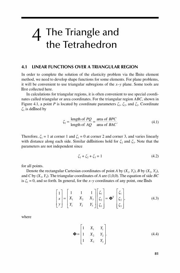
81
4 The Triangle and the Tetrahedron
4.1 lInear functIonS over a trIangular regIon
In order to complete the solution of the elasticity problem via the finite element method, we need to develop shape functions for some elements. For plane problems, it will be convenient to use triangular subregions of the x–y plane. Some tools are first collected here.
In calculations for triangular regions, it is often convenient to use special coordi-nates called triangular or area coordinates. For the triangular region ABC, shown in Figure 4.1, a point P is located by coordinate parameters ζ1, ζ2, and ζ3. Coordinate ζ1 is defined by
ζ1 = =length of
length ofarea ofarea of
PQAQ
BPCBAC
.
(4.1)
Therefore, ζ1 = 1 at corner 1 and ζ1 = 0 at corner 2 and corner 3, and varies linearly with distance along each side. Similar definitions hold for ζ2 and ζ3. Note that the parameters are not independent since
ζ1 + ζ2 + ζ3 = 1 (4.2)
for all points.Denote the rectangular Cartesian coordinates of point A by (X1, Y1), B by (X2, Y2),
and C by (X3, Y3). The triangular coordinates of A are (1,0,0). The equation of side BC is ζ1 = 0, and so forth. In general, for the x–y coordinates of any point, one finds
1 1 1 1
1 2 3
1 2 3
1
2
3
xy
X X X
Y Y Y
=
ζ
ζ
ζ
=
ΦΦT
ζ
ζ
ζ
1
2
3
,
(4.3)
where
ΦΦ =
1
1
1
1 1
2 2
3 3
X Y
X Y
X Y
.
(4.4)

82 The Finite Element Method for Mechanics of Solids with ANSYS Applications
The inverse transformation is
ζ
ζ
ζ
1
2
3
1
=
−( ) .ΦΦ 1 T xy
(4.5)
The inverse of the matrix Φ is
ΦΦ− =
1
1 2 3
1 2 3
1 2 3
12
2 2 2
a
A A A
a a a
b b b
,
(4.6)
where
2 2 21 2 3 3 2 2 3 1 1 3 3 1 2 2 1
1 2
A X Y X Y A X Y X Y A X Y X Y
a Y
= − = − = −=
, , ,
−− = − = −= − = − = −
Y a Y Y a Y Y
b X X b X X b X3 2 3 1 3 1 2
1 3 2 2 1 3 3 2
, , ,
, , XX1,
(4.7)
and
a
X Y
X Y
X Y
= 12
1
1
1
1 1
2 2
3 3
.
(4.8)
The determinant is positive if the nodes are numbered counterclockwise, and a is the area of the triangle. The matrix Φ–1 depends only on the geometry of the triangle. Once the shape of the triangle is specified, Φ–1 can be calculated. It does not depend on the absolute position in space since only the differences in the nodal coordinates occur in 4.7.
y
x
P
AB
C
Q
fIgure 4.1 Triangular coordinates.

The Triangle and the Tetrahedron 83
One major importance of triangular coordinates is the identity
ζ ζ ζ1 2 3 2
2m n p Am n p
m n pad∫∫ =
+ + +! ! !
( )!,
(4.9)
where m, n, and p are exponents, not indices. This makes integration of polynomials over the triangular region an easy task.
Now, consider the general linear function
f x y c c x c y x y ci( , ) { }= + + =
1 2 3 1 .
(4.10)
The values of f at points A, B, and C are
f
f
f
X Y
X Y
X Y
c1
2
3
1 1
2 2
3 3
1
1
1
=
11
2
3
c
c
f ci i
=or { } { }.ΦΦ
(4.11)
Therefore,
{ci} = Φ–1{fi}. (4.12)
Thus, function 4.10 can be expressed in terms of its values at the corners:
f(x,y) = [1 x y]Φ–1{fi}. (4.13)
In the area coordinates, by 4.5,
f(x,y) = ζ1f1 + ζ2f2 + ζ3f3. (4.14)
Thus, the general linear function f(x,y) is expressed in a very simple way in terms of its values at the nodes by using the triangular coordinates.
We automatically achieve the task of constructing a continuous displacement field. To show this, let us consider a pair of triangles (Figure 4.2) and a general linear function over each one. Along side BC of triangle 1, we have ζ1 = 0 and
AB
C
D
2
1
fIgure 4.2 Two adjacent triangles.

84 The Finite Element Method for Mechanics of Solids with ANSYS Applications
f(0,ζ2,ζ3) = ζ2 f2 + ζ3 f3 = ζ2 f2 + (1 – ζ2)f3. (4.15)
Thus, f(x,y) varies linearly along the edge BC and values of f along the side depends only on values of f at the nodes lying on that side. If we consider another linear func-tion defined in a similar manner over triangle 2 that shares the edge BC with triangle 1, we again find that f varies linearly from B to C and depends only on values at B and C. The two functions must be equal along line BC because both are linear and have the same values at B and C. Function f is therefore continuous across the element boundary, that is, ζi are shape functions for the three-node triangle.
By dividing any region into a number of such triangles, we can construct a continu-ous piecewise linear function over the region. Graphically, this function is an assembly of inclined planes joined above the edge of the triangles. In the limit, as the size of each triangle tends to zero, we can approximate any continuous function over the region as closely as we like by such piecewise linear functions. We can therefore use this repre-sentation to approximate each component of displacement in the plane problem. The fundamental unknowns then become the nodal values rather than the entire function. Instead of solving for a function, we have only to find a finite number of real numbers.
4.2 trIangular eleMent for plane StreSS and plane StraIn
The triangle has three corner nodes (Figure 4.3) with displacement components (Ui,Vi). The components u1 and u2 of displacement can be represented within a typi-cal element by linear function 4.13:
u x y U U U
u x y V
11
1 1 2 2 3 3
21
1 1
1
1
= = + +
= = +
−
−
[ ] ,
[ ]
ΦΦ
ΦΦ
U
V
ζ ζ ζ
ζ ζ22 2 3 3V V+ ζ , (4.16)
where
U
V
=
=
U U U
V V V
1 2 3
1 2 3
T
T
,
.
(4.17)
U2
U1
U3
V2V1
V3y
x
3
21
fIgure 4.3 Triangular element with three nodes.

The Triangle and the Tetrahedron 85
Differentiating with respect to x and y gives
u
aa a a1 1
11 2 30 1 0
12, [ ] ,= =
−ΦΦ U U
(4.18)
u
ab b b1 2
11 2 30 0 1
12, [ ] ,= =
−ΦΦ U U
(4.19)
u
aa a a2 1
11 2 30 1 0
12, [ ] ,= =
−ΦΦ V V
(4.20)
u
ab b b2 2
11 2 30 0 1
12, [ ] .= =
−ΦΦ V V
(4.21)
Uk and Vk are the x and y components of displacement of the kth node. From 2.27 using 4.18 to 4.21 and 4.4, with γ12 = 2ε12,
ε = AD (4.22)
where
εε =
=
ε
ε
γ
11
22
12
, ,D UV
(4.23)
and
A =
=12
0 0 0
0 0 011
1
2
2
3
3
1
1
2
2
3
3
a
a
b
a
b
a
b
b
a
b
a
b
a22a
a
b
b a
k
k
k k
0
0 ,
(4.24)
where ai and bi are given by 4.7.For an isotropic material with no temperature change, from 2.81,
τ = Cε, (4.25)
where
ττ =
τ
τ
τ
11
22
12
.
(4.26)
86 The Finite Element Method for Mechanics of Solids with ANSYS Applications
For plane strain,
C =+
+
2 0
2 0
0 0
µ λ λλ µ λ
µ.
(4.27)
For plane stress,
C =−
−
21
1 01 0
0 0 1 2
µν
νν
ν( )
.
/
(4.28)
For the isotropic material in plane stress or plane strain, C has the form
C =
C C
C C
C
11 12
12 11
33
0
0
0 0
.
(4.29)
From 4.22 and 4.25,
τ = BD, (4.30)
where
B = CA. (4.31)
From 3.24, applied to two dimensions, the element stiffness matrix is
k B A= ∫ T daR
.
(4.32)
Since A and B are constant, one finds
k = aATCA (4.33)
where a is the area of the element. In this case, k is a 6 × 6 matrix:
U V
k k kk k
=
uu uv
vu vv
(4.34)
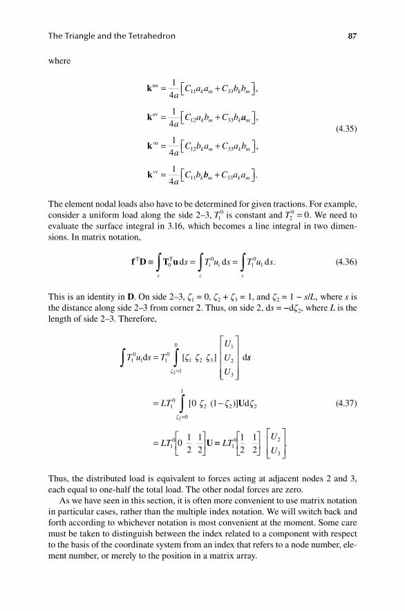
The Triangle and the Tetrahedron 87
where
k
k
uuk m k m
uvk m k
aC a a C b b
aC a b C b
= +
= +
14
14
11 33
12 33
,
aa
aC b a C a b
aC b
m
vuk m k m
vvk
= +
=
,
,k
k
14
14
12 33
11 bb C a am k m+ 33 .
(4.35)
The element nodal loads also have to be determined for given tractions. For example, consider a uniform load along the side 2–3, T1
0 is constant and T20 0= . We need to
evaluate the surface integral in 3.16, which becomes a line integral in two dimen-sions. In matrix notation,
f D T uT T d d d≡ = =∫ ∫ ∫00
10
1s T u s T u si i
c c c
.
(4.36)
This is an identity in D. On side 2–3, ζ1 = 0, ζ2 + ζ3 = 1, and ζ2 = 1 − s/L, where s is the distance along side 2–3 from corner 2. Thus, on side 2, ds = −dζ2, where L is the length of side 2–3. Therefore,
T u s T
U
U
U10
1 10
1 2 3
1
0 1
2
32
∫ ∫=
=
d d[ ]ζ ζ ζζ
ss
LT
LT
= −
=
=∫1
02
0
1
2 2
10
0 1
012
12
2
[ ( )] dζ ζ ζζ
U
U ==
LTU
U10 2
3
12
12
.
(4.37)
Thus, the distributed load is equivalent to forces acting at adjacent nodes 2 and 3, each equal to one-half the total load. The other nodal forces are zero.
As we have seen in this section, it is often more convenient to use matrix notation in particular cases, rather than the multiple index notation. We will switch back and forth according to whichever notation is most convenient at the moment. Some care must be taken to distinguish between the index related to a component with respect to the basis of the coordinate system from an index that refers to a node number, ele-ment number, or merely to the position in a matrix array.

88 The Finite Element Method for Mechanics of Solids with ANSYS Applications
In the notation of 3.19, the shape functions corresponding to 4.16 and 4.17 are
Na
A a x b y N
N Na
A a x
11 1 1 1 21
12 22 1 1
12
2 0
01
22
= + + =
= = +
( ),
, ( ++
= + + =
= =
b y
Na
A a x b y N
N Na
1
13 2 2 2 23
14 24
12
2 0
01
2
),
( ), ,
, (( ),
( ), ,
2
12
2 0
0
2 2 2
15 3 3 3 25
16
A a x b y
Na
A a x b y N
N
+ +
= + + =
= ,, ( ),Na
A a x b y26 3 3 3
12
2= + +
(4.38)
The geometric factors Aαβk defined by 3.4 can be read off from 4.38 as elements from matrix A. The coefficients cαβγδ are elements of matrix C. The coefficients Bαβk are elements of matrix B. Elements of matrix k are exactly the kIJ
m of 3.11, except that the explicit indication of element number by the index m has been omitted in this section.
4.3 plane quadrIlateral froM four trIangleS
A quadrilateral element is readily formed from four triangles with a common node at the centroid of the quadrilateral. The common node can then be eliminated if there is no body force.
Consider a typical quadrilateral region subdivided into four triangles as shown in Figure 4.4. Node number 5 can be placed at any interior point, but it is usually placed at the centroid of the quadrilateral and the coordinates (X5,Y5) are calculated from the coordinates of nodes 1–4.
The stiffness matrix for each triangle is given by 4.33. The 10 × 10 stiffness matrix of the complete quadrilateral is then formed by merging the element matrices as described in Section 4.4. Let us suppose that there are no forces associated with node 5. Then, Equation 3.18 for the quadrilateral becomes
y
x2
34
1
5
fIgure 4.4 Four-triangle assembly.

The Triangle and the Tetrahedron 89
k k
k k11 12
21 22
1
1
2
2
3
3
4
4
5
5
U
V
U
V
U
V
U
V
U
V
=
FX
FY
FX
FY
FX
FY
1
1
2
2
3
3
FFX
FY4
4
00
,
(4.39)
where FXk and FYk are the node forces, and the stiffness matrix for the quadrilat-eral has been partitioned into four submatrices. The submatrix k22 is 2 × 2 and so forth. The last two equations can be used to solve for the displacements (U5, V5) of node 5:
U
V5
5221
21
= − −k k D,
(4.40)
where the fundamental nodal displacements and nodal forces are
D
F
=
=
U V U V U V U V
FX FY FX FY FX FY FX
1 1 2 2 3 3 4 4
1 1 2 2 3 3 4
T
,
FFY4
T
.
(4.41)
Next, use 4.40 to eliminate (U5, V5) from the first eight equations of 4.39 to obtain
KD = F, (4.42)
where
K k k k k= − −11 12 22
121. (4.43)
and F is the column matrix of forces acting at nodes 1 to 4. K, an 8 × 8 matrix, is the stiffness matrix of the quadrilateral shown in Figure 4.5.
One may now use the quadrilateral as a basic finite element with a stiffness matrix given by 4.43. The region is divided into quadrilaterals (and possibly tri-angles also) and the global stiffness matrix is formed by merging the element

90 The Finite Element Method for Mechanics of Solids with ANSYS Applications
matrices. Note that the stress is still approximated as constant within each trian-gular subregion.
This process of elimination of unloaded internal nodes to obtain a stiffness matrix for a patch of elements is called static condensation. The patch of elements can then be used as a building block for a finite element model, just as one uses a single element.
Static condensation may be used in other ways. For example, shape functions are sometimes used in conjunction with parameters that are not interpreted as nodal val-ues of the displacement. Such nodeless parameters may then be eliminated by static condensation to obtain the stiffness matrix for the element.
4.3.1 Square eleMent forMed froM four triangleS
The nodes and elements are numbered as shown in Figure 4.6. The nodal coor-dinates for each element to be used in Equation 4.7 are shown in Table 4.1. The area of each element is h2/4. The geometric parameters in 4.24 are shown in Table 4.2.
For ν = 1/3, μ = 3E/8, from 4.28 the matrix C for plane stress is
C =
µ3 1 01 3 00 0 1
.
(4.44)
The stiffness matrix for each element is calculated from 4.33:
y4
3
21x
fIgure 4.5 Quadrilateral formed from four triangles.
x
4 33
45 2
21
1
y
h
h
fIgure 4.6 Square from four triangles.

The Triangle and the Tetrahedron 91
U V U V U V1 1 2 2 5 5
1
4
4 2 2 0 2 22 4 0 2 2 62 0 4 2 2 20 2 2
k =
− − −− −
− − −−
µ44 2 6
2 2 2 2 4 02 6 2 6 0 12
−− − −− − −
,
U V U V U V3 3 4 4 5 5
3
4
4 2 2 0 2 22 4 0 2 2 62 0 4 2 2 20 2 2
k =
− − −− −
− − −−
µ44 2 6
2 2 2 2 4 02 6 2 6 0 12
−− − −− − −
,
(4.45)
U V U V U V2 2 3 3 5 5
2
4
4 2 2 0 6 22 4 0 2 2 22 0 4 2 6 20 2 2 4
k =
− −− − −
− −−
µ−− −
− − −− − −
2 26 2 6 2 12 02 2 2 2 0 4
,
U V U V U V4 4 1 1 5 5
4
4
4 2 2 0 6 22 4 0 2 2 22 0 4 2 6 20 2 2 4
k =
− −− − −
− −−
µ−− −
− − −− − −
2 26 2 6 2 12 02 2 2 2 0 4
.
(4.46)
taBle 4.1element geometry
element nodes X1/h X2/h X3/h Y1/h Y2/h Y3/h
1 1–2–5 0 1 1/2 0 0 1/2
2 2–3–5 1 1 1/2 0 1 1/2
3 3–4–5 1 0 1/2 1 1 1/2
4 4–1–5 0 0 1/2 1 0 1/2
taBle 4.2element parameters
element nodes a1/h a2/h a3/h b1/h b2/h b3/h
1 1–2–5 −1/2 +1/2 0 −1/2 −1/2 +1
2 2–3–5 +1/2 +1/2 −1 −1/2 +1/2 0
3 3–4–5 +1/2 −1/2 0 +1/2 +1/2 −1
4 4–1–5 −1/2 −1/2 +1 +1/2 −1/2 0
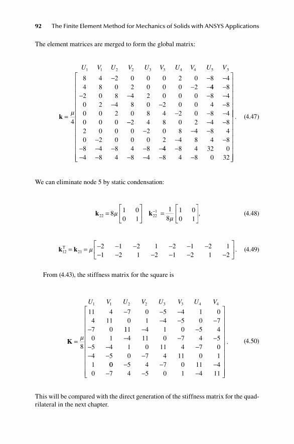
92 The Finite Element Method for Mechanics of Solids with ANSYS Applications
The element matrices are merged to form the global matrix:
U V U V U V U V U V1 1 2 2 3 3 4 4 5 5
4
8 4 2 0 0 0 2 0 8 44 8 0 2 0 0 0 2
k =
− − −− −
µ
44 82 0 8 4 2 0 0 0 8 40 2 4 8 0 2 0 0 4 80 0 2 0 8 4 2 0 8 40 0 0
−− − − −
− − −− − −
−− − −− − −
− − −− − − − −
2 4 8 0 2 4 82 0 0 0 2 0 8 4 8 40 2 0 0 0 2 4 8 4 88 4 8 4 8 44 8 4 32 04 8 4 8 4 8 4 8 0 32
−− − − − − −
.
(4.47)
We can eliminate node 5 by static condensation:
k k22 2218 1 0
0 1
18
1 00 1
=
=
−µ
µ, (4.48)
k k12 212 1 2 1 2 1 2 11 2 1 2 1 2 1 2
T = = − − − − − −− − − − − −
µ . (4.49)
From (4.43), the stiffness matrix for the square is
U V U V U V U V1 1 2 2 3 3 4 4
8
11 4 7 0 5 4 1 04 11 0 1 4 5 0 77 0
K =
− − −− − −
−µ
111 4 1 0 5 40 1 4 11 0 7 4 55 4 1 0 11 4 7 04 5 0 7 4 11 0 11
− −− − −
− − −− − −
00 5 4 7 0 11 40 7 4 5 0 1 4 11
− − −− − −
.
(4.50)
This will be compared with the direct generation of the stiffness matrix for the quad-rilateral in the next chapter.
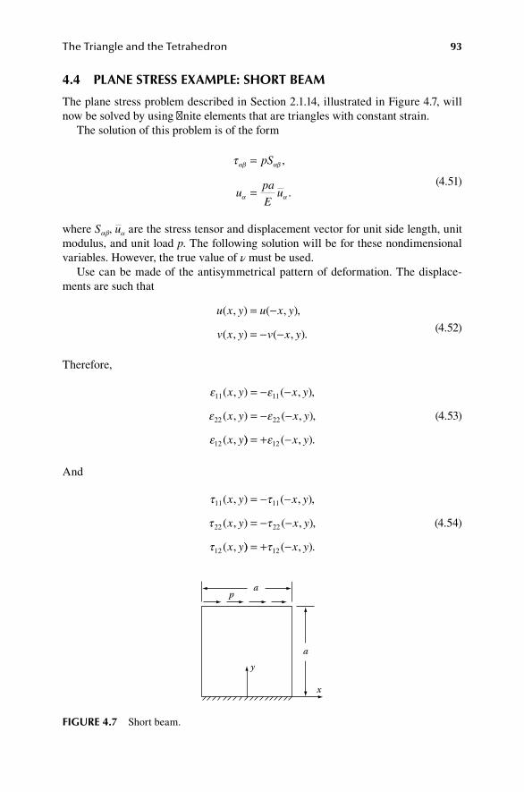
The Triangle and the Tetrahedron 93
4.4 plane StreSS exaMple: Short BeaM
The plane stress problem described in Section 2.1.14, illustrated in Figure 4.7, will now be solved by using finite elements that are triangles with constant strain.
The solution of this problem is of the form
τ αβ αβ
α α
=
=
pS
upa
Eu
,
.
(4.51)
where Sαβ, uα are the stress tensor and displacement vector for unit side length, unit modulus, and unit load p. The following solution will be for these nondimensional variables. However, the true value of ν must be used.
Use can be made of the antisymmetrical pattern of deformation. The displace-ments are such that
u x y u x y
v x y v x y
( , ) ( , ),
( , ) ( , ).
= −
= − − (4.52)
Therefore,
ε ε
ε ε
ε
11 11
22 22
12
( , ) ( , ),
( , ) ( , ),
( ,
x y x y
x y x y
x y
= − −
= − −
)) ( , ).= + −ε12 x y
(4.53)
And
τ τ
τ τ
τ
11 11
22 22
12
( , ) ( , ),
( , ) ( , ),
( ,
x y x y
x y x y
x y
= − −
= − −
)) ( , ).= + −τ12 x y
(4.54)
x
y
a
ap
fIgure 4.7 Short beam.

94 The Finite Element Method for Mechanics of Solids with ANSYS Applications
Along the line x = 0, we have the antisymmetry conditions: u2 = 0, τ11 = τ22 = 0. Therefore, we only need to consider one-half of the region and use the symmetry conditions as boundary conditions. However, in the following example analysis, the entire region is retained for illustration.
A typical element layout is shown in Figure 4.8. In general, there are N segments per side. The nodes on the bottom edge have zero displacement. The generalized forces for nodes on the top edge are (0, 1/N), except for the corner nodes where they are 1/2 as much. Other generalized forces are zero. The calculated x displacement of corner C is shown in Table 4.2 for ν = 1/3.
The calculated displacement is always too small but increases monotonically to the true solution as the number of elements increases. Figure 4.9 shows the calcu-lated displacement as a function of the number of divisions in this layout.
The stress varies smoothly in the exact solution. However, in the finite element model, the strains and therefore the stresses are constant throughout each triangle. Some interpolation of the calculated values is therefore necessary. A common method of interpreting the finite element analysis is to take the calculated values to
7.5
7
6.5
6
5.5
5
4.5
40 5 10 15 20 25
Disp
lace
men
t
Divisions
fIgure 4.9 Convergence toward the exact solution.
1/81/41/41/41/8C
fIgure 4.8 Element layout.

The Triangle and the Tetrahedron 95
be the stress state at the centroid of the triangle. Figures 4.10 through 4.13 show the results for 1600 triangles using that interpretation.
The exact solution to this simple-looking problem is unknown. The stress state distant from the top and bottom edges was estimated in Section 2.1.14, Equations 2.52 and 2.53. Looking at Figure 4.10, one sees very good agreement with this ele-mentary theory on the interior of the region.
As expected, Figure 4.11 shows that the elementary theory is not satisfactory near the support where the stress distribution depends strongly on the details of the sup-port condition. Figure 4.12 shows that the elementary theory is also not satisfactory near the loaded edge, where the stress distribution depends strongly on the details of the load distribution.
We have analyzed the situation in the corner x = 0, y = 0, as given by 2.58. We expect a singularity (infinite stress) at the corners where the free and fixed boundaries join. The effect of the singularity can be seen in Figures 4.11 and 4.13. The infinite stresses at those points are, of course, never found via a numerical analysis. For each finer element mesh, one simply finds higher and higher stresses near the corners.
3
2
1
0
–1
–2
–3
0 0.2 0.4 0.6 0.8 10.1 0.3 0.5 0.7 0.9
SY
SX
SXY
fIgure 4.10 Stress at y = 0.5083.
0 0.20.1 0.4 0.6 10.3 0.5 0.7 0.8 0.9
8
6
4
2
0
–2
–4
–6
–8SY
SX
SXY
fIgure 4.11 Stress at y = 0.0083.
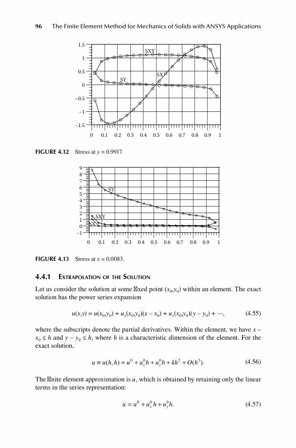
96 The Finite Element Method for Mechanics of Solids with ANSYS Applications
4.4.1 extrapolation of the Solution
Let us consider the solution at some fixed point (x0,y0) within an element. The exact solution has the power series expansion
u(x,y) = u(x0,y0) + ux(x0,y0)(x – x0) + uy(x0,y0)(y – y0) + ⋯, (4.55)
where the subscripts denote the partial derivatives. Within the element, we have x – x0 ≤ h and y – y0 ≤ h, where h is a characteristic dimension of the element. For the exact solution,
u u h h u u h u h kh O hx y≡ = + + + +( , ) ( ).0 0 0 2 3 (4.56)
The finite element approximation is u, which is obtained by retaining only the linear terms in the series representation:
u u u h u hx y= + +0 0 0 . (4.57)
9876543210
–1
0 .1 0.2 0.4 0.6 0.8 10 0.3 0.5 0.7 0.9
SXSXY
SY
fIgure 4.13 Stress at x = 0.0083.
1.5
1
0.5
0
–0.5
–1
–1.5
0 0.2 0.4 0.6 0.8 10.1 0.3 0.5 0.7 0.9
SXY
SYSX
fIgure 4.12 Stress at y = 0.9917.

The Triangle and the Tetrahedron 97
The finite element approximation therefore differs from the exact solution by
u u kh O h− = +2 3( ). (4.58)
Let h be a small number and denote the finite element solution for some value h1 by u1, and by u2 for h2. Neglecting the higher-order terms,
u u
u u
h
h
−−
=2
1
2 2
1
α α, .
(4.59)
Thus,
u
u u
22
121
−−
αα
.
(4.60)
This formula can be used to estimate the exact solution from the finite element cal-culations. From the data in Table 4.3, we have the following estimate for u2 7 372= . , u1 7 350= . , and α = 20/25 = 0.8 is
u
7 372 0 8 7 350
1 0 87 41
2
2
. ( . ) .
( . ).
−−
= .
(4.61)
We will see later from a more detailed finite element solution that the exact answer is still larger.
4.5 lInear StraIn trIangleS
We have seen in Section 4.1 how a general linear expression for displacement led naturally to a triangular with three corner nodes. The strains in that triangle are con-stant. Let us now consider a general quadratic expression for displacement. We will see that the quadratic expression leads naturally to a six-node triangle.
taBle 4.3convergence
Segments per Side no. of nodes
no. of triangles
no. of rectangles
corner displacement
1 5 4 1 4.444
2 13 16 4 5.785
4 41 64 16 6.735
10 221 400 100 7.223
20 841 1600 400 7.350
25 1301 2500 625 7.372
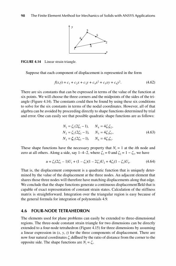
98 The Finite Element Method for Mechanics of Solids with ANSYS Applications
Suppose that each component of displacement is represented in the form
f(x,y) = c1 + c2x + c3y + c4x2 + c5xy + c6y2. (4.62)
There are six constants that can be expressed in terms of the value of the function at six points. We will choose the three corners and the midpoints of the sides of the tri-angle (Figure 4.14). The constants could then be found by using these six conditions to solve for the six constants in terms of the nodal coordinates. However, all of that algebra can be avoided by proceeding directly to shape functions determined by trial and error. One can easily see that possible quadratic shape functions are as follows:
N N
N N
N
1 1 1 4 1 2
2 2 2 5 2 3
3
2 1 4
2 1 4
= − == − ==
ζ ζ ζ ζ
ζ ζ ζ ζ
( ), ,
( ), ,
ζζ ζ ζ ζ3 3 6 3 12 1 4( ), .− =N
(4.63)
These shape functions have the necessary property that Ni = 1 at the ith node and zero at all others. Along a side, say 1–4–2, where ζ3 = 0 and ζ2 = 1 − ζ1, we have
u = ζ1(2ζ1 – 1)U1 + (1 – ζ1)(1 – 2ζ1)U2 + 4ζ1(1 – ζ1)U4. (4.64)
That is, the displacement component is a quadratic function that is uniquely deter-mined by the value of the displacement at the three nodes. An adjacent element that shares those three nodes will therefore have matching displacements along that edge. We conclude that the shape functions generate a continuous displacement field that is capable of exact representation of constant strain states. Calculation of the stiffness matrix is straightforward. Integration over the triangular region is easy because of the general formula for integration of polynomials 4.9.
4.6 four-node tetrahedron
The elements used for plane problems can easily be extended to three-dimensional regions. The three-node constant strain triangle for two dimensions can be directly extended to a four-node tetrahedron (Figure 4.15) for three dimensions by assuming a linear expression in (x, y, z) for the three components of displacement. There are now four natural coordinates ζi defined by the ratio of distance from the corner to the opposite side. The shape functions are Ni = ζi.
x
24
1
6
35
y
fIgure 4.14 Linear strain triangle.

The Triangle and the Tetrahedron 99
4.7 ten-node tetrahedron
The 2D triangle with mid-side nodes becomes the 10-node tetrahedron in three dimensions (Figure 4.16).
The shape functions are easily generated:
nodes 1, 2, 3, 4: Ni = ζi(2ζi – 1) nodes 5, 6, 7: N5 = ζ1ζ2, N6 = ζ2ζ3, N7 = ζ3ζ1
nodes 8.9.10: N8 = ζ1ζ4, N9 = ζ2ζ4, N10 = ζ3ζ4
See ANSYS elements Solid 92 and 187.
4.8 proBleMS
1. For the example problem shown in Figure 4.8, determine the force matrix F for a layout of triangles with N = 3 segments per side. You can label the elements and nodes in any convenient way.
2. Derive the nodal forces for a uniform body force b1 = 1 for a three-node triangular element in plane stress. Show your answer on a diagram.
3. For the triangle element with linearly varying load T1 as shown in Figure 4.17, determine the element force matrix.
4. Consider the layout of triangular elements for plane stress with eight ele-ments and nine nodes as shown in Figure 4.18.
Mark an X for the terms that may be nonzero and a 0 for the terms that must be zero in the first row of the global stiffness matrix.
4
3
2
1
fIgure 4.15 The four-node tetrahedron.
3
6
251
8
7
9
104
fIgure 4.16 The 10-node tetrahedron.
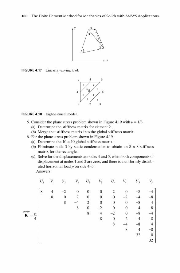
100 The Finite Element Method for Mechanics of Solids with ANSYS Applications
5. Consider the plane stress problem shown in Figure 4.19 with ν = 1/3.(a) Determine the stiffness matrix for element 2.(b) Merge that stiffness matrix into the global stiffness matrix.
6. For the plane stress problem shown in Figure 4.19,(a) Determine the 10 × 10 global stiffness matrix.(b) Eliminate node 3 by static condensation to obtain an 8 × 8 stiffness
matrix for the rectangle.(c) Solve for the displacements at nodes 4 and 5, when both components of
displacement at nodes 1 and 2 are zero, and there is a uniformly distrib-uted horizontal load p on side 4–5.
Answers:
U V U V U V U V U V1 1 2 2 3 3 4 4 5 5
10 10
4
8 4 2 0 0 0 2 0 8 48 0 2 0 0
K×
=
− − −
µ
00 2 4 88 4 2 0 0 0 8 4
8 0 2 0 0 4 88 4 2 0 8 4
8 0 2 4 88 4
− − −− −
− −− − −
− −− −88 4
8 4 832 0
32
−
1 2 3
4 5 6
7 8 9
1 2
3 4
5 67 8
fIgure 4.18 Eight-element model.
x
y q
3
12
fIgure 4.17 Linearly varying load.
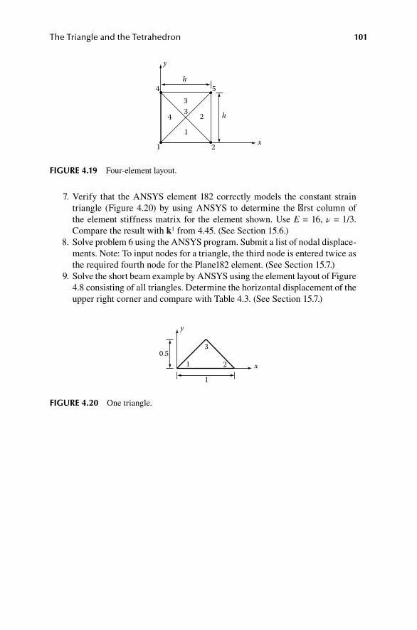
The Triangle and the Tetrahedron 101
7. Verify that the ANSYS element 182 correctly models the constant strain triangle (Figure 4.20) by using ANSYS to determine the first column of the element stiffness matrix for the element shown. Use E = 16, ν = 1/3. Compare the result with k1 from 4.45. (See Section 15.6.)
8. Solve problem 6 using the ANSYS program. Submit a list of nodal displace-ments. Note: To input nodes for a triangle, the third node is entered twice as the required fourth node for the Plane182 element. (See Section 15.7.)
9. Solve the short beam example by ANSYS using the element layout of Figure 4.8 consisting of all triangles. Determine the horizontal displacement of the upper right corner and compare with Table 4.3. (See Section 15.7.)
x21
h
h54
3
43
2
1
y
fIgure 4.19 Four-element layout.
x
y
3
21
1
0.5
fIgure 4.20 One triangle.

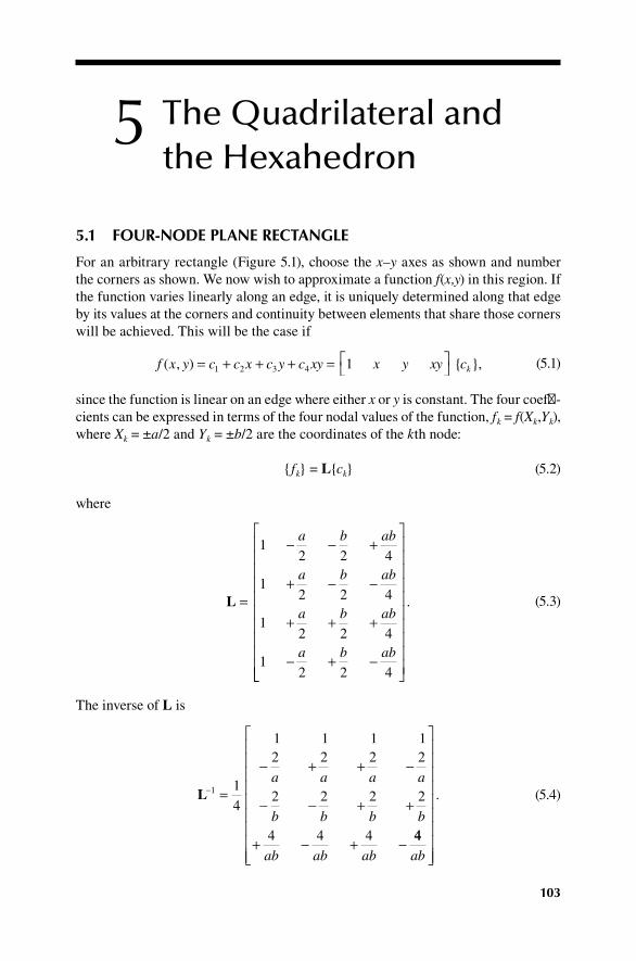
103
5 The Quadrilateral and the Hexahedron
5.1 four-node plane rectangle
For an arbitrary rectangle (Figure 5.1), choose the x–y axes as shown and number the corners as shown. We now wish to approximate a function f(x,y) in this region. If the function varies linearly along an edge, it is uniquely determined along that edge by its values at the corners and continuity between elements that share those corners will be achieved. This will be the case if
f x y c c x c y c xy x y xy ck( , ) { },= + + + =
1 2 3 4 1
(5.1)
since the function is linear on an edge where either x or y is constant. The four coeffi-cients can be expressed in terms of the four nodal values of the function, fk = f(Xk,Yk), where Xk = ±a/2 and Yk = ±b/2 are the coordinates of the kth node:
{fk} = L{ck} (5.2)
where
L =
− − +
+ − −
+ + +
− + −
1
2 2 4
12 2 4
12 2 4
12 2 4
a b ab
a b ab
a b ab
a b ab
.
(5.3)
The inverse of L is
L− =
− + + −
− − + +
+ − + −
1 14
1 1 1 12 2 2 2
2 2 2 2
4 4 4
a a a a
b b b b
ab ab ab
44ab
.
(5.4)

104 The Finite Element Method for Mechanics of Solids with ANSYS Applications
Therefore,
f x y x y xy f fk k( , ) { } { }=
=−1 1L N
(5.5)
where
N =
− − +
+ − −
+ + +
14
12 2 4
12 2 4
12 2 4
x
a
y
b
xy
abx
a
y
b
xy
abx
a
y
b
xy
aabx
a
y
b
xy
ab1
2 2 4− + −
.
(5.6)
It is convenient to use the nondimensional coordinates
ξ η ξ η= = − ≤ ≤ − ≤ ≤2 2
1 1 1 1x
a
y
b, , , .
(5.7)
Then,
N N
N
1 2
3
14
1 114
1 1
14
1 1
≡ − − ≡ + −
≡ + +
( )( ), ( )( ),
( )( )
ξ η ξ η
ξ η ,, ( )( ),N4
14
1 1≡ − +ξ η
(5.8)
and
f x y N f N f N f N f( , ) ( , ) ( , ) ( , ) ( , )= + + + =1 1 2 2 3 3 4 4ξ η ξ η ξ η ξ η NN fk k
k=∑
1
4
. (5.9)
121
34
2
2
2 2 1 1
1ƞ
ξb
b
a a
yx
fIgure 5.1 Four-node element.

The Quadrilateral and the Hexahedron 105
The formulas for Nk can be written concisely as
Nk k k= + +1
41 1( )( )ξ ξ η η
(5.10)
where ξk and ηk are the coordinates of the nodes in the ξ – η system. The functions Nk are called shape functions or interpolation functions. They have the property
Nk(ξm,ηm) = δkm. (5.11)
The functions in 5.10 are known as the serendipity functions because they could have been easily found by trial and error. Recall that any functions that satisfy the following three requirements may be used as shape functions:
(1) The shape function for a degree of freedom (DOF) must have the value of 1 for that DOF and 0 for all others: Nk(ξm,ηm) = δkm.
(2) The displacement field generated by the shape functions must be continuous between elements.
(3) The representation of displacement within an element must contain the lower-order terms of the power series representation for the function so that arbitrary constant strain states can be represented.
It does not matter how we discover the functions. We will subsequently generate other elements by a judicious choice of the shape functions.
We will need the derivatives of the shape functions:
∂∂
= + ∂∂
= +N Nkk k
kk kξ
ξ η ηη
η ξ ξ14
114
1( ), ( ).
(5.12)
Hence,
∂∂
= ∂∂
= + ≡
∂∂
= ∂∂
N
x
N
x aA
N
y
N
k kk k k
k k
ξξ
ξ η η
ηη
dd
dd
12
1 1( ) ,
yy bAk k k= + ≡1
21 2η ξ ξ( ) .
(5.13)
Therefore,
∂∂
= ∂∂
= + = { }
∂
= =∑ ∑f
x
N
xf
af f
f
kk
k
k k k
k
k
1
4
1
4
1
12
1ξ η η( ) ,A
∂∂= ∂
∂= + = { }
= =∑ ∑y
N
yf
bf fk
k
k
k k k k
k1
4
2
1
41
21η ξ ξ( ) ,A
(5.14)

106 The Finite Element Method for Mechanics of Solids with ANSYS Applications
where
A
A
11
22
12
1
12
= = +
= =
Aa
Ab
k k k
k k
ξ η η
η
( ) ,
(11 +
ξ ξk ) .
(5.15)
For a plane region, we approximate u(x,y) and v(x,y) by 5.9:
u N U v N Vk k
k
k k
k
= == =
∑ ∑1
4
1
4
, ,
(5.16)
where Uk denotes the value of u(x,y) at corner k, whereas Vk denotes the value of v(x,y) at corner k. That is,
u = ND (5.17)
where
u N0
0D=
=
=
u
v
N
N
U
V
k
k
k
k, ,
.
(5.18)
From 2.1, 5.14, and 5.16,
εε ==ε
ε
γ
11
22
12
= AD
(5.19)
where
A
A 0
0 A
A A
A A=
=
=
1
2
2 1
11
22, , .A Ak k
(5.20)
Equation 5.19 is of the same form as 4.22, but here A is a 3 × 8 matrix since there are eight displacement parameters, and the components of A are not constant. From 3.24, the stiffness matrix for the plane rectangle is
k A CA A CA= =∫∫ ∫∫=−=−
T Td d d dx yab
41
1
1
1
ξ ηηξ
.
(5.21)
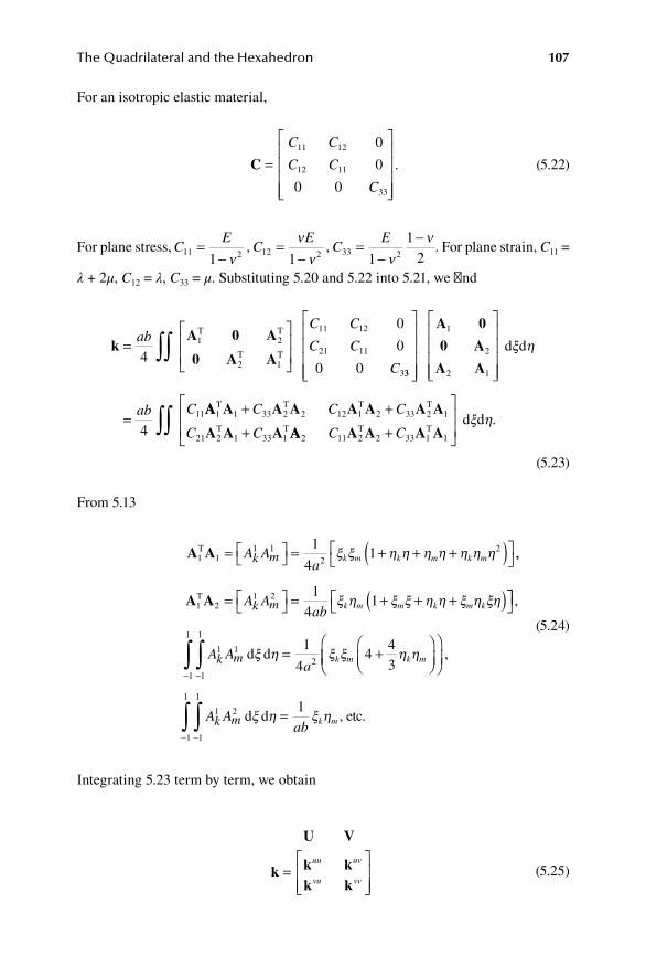
The Quadrilateral and the Hexahedron 107
For an isotropic elastic material,
C =
C C
C C
C
11 12
12 11
33
0
0
0 0
.
(5.22)
For plane stress, CE
CE
CE
11 2 12 2 33 21 1 1
12
=−
=−
=−
−ν
νν ν
ν, , . For plane strain, C11 =
λ + 2μ, C12 = λ, C33 = μ. Substituting 5.20 and 5.22 into 5.21, we find
kA 0 A
0 A A=
∫∫ab
C C
C C
C4
0
0
0 0
1 2
2 1
11 12
21 11
3
T T
T T
33
1
2
2 1
11
4
=
A 0
0 A
A A
d dξ η
ab C AA A A A A A A A
A A A1 1 33 2 2 12 1 2 33 2 1
21 2 1 33 1
T T T T
T T
+ +
+
C C C
C C AA A A A A2 11 2 2 33 1 1C CT Td d
+
∫∫ ξ η.
(5.23)
From 5.13
A A1 11 1
221
41T = = + + +( )
A A
ak m k m k m k mξ ξ η η η η η η η ,,
A A1 21 2 1
41T = = + + +( )A A
abk m k m m k m kξ η ξ ξ η η ξ η ξη
= +
−−∫∫
,
A Aak m k m k m
1 1
1
1
1
1
2
1
44
43
d dξ η ξ ξ η η
=−−∫∫
,
,A Aabk m k m
1 2
1
1
1
11
d d etc.ξ η ξ η
(5.24)
Integrating 5.23 term by term, we obtain
U V
k k kk k
=
uu uv
vu vv
(5.25)
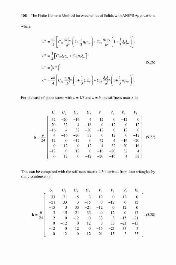
108 The Finite Element Method for Mechanics of Solids with ANSYS Applications
where
kuu k mk m
k mk
abC
aC
b= +
+ +4
113
11311 2 33 2
ξ ξη η
η ηξ ξmm
uvk m k m
vu u
C C
= +
=
,
,k
k k
14 12 33ξ η η ξ
vv
vv k mk m
k mabC
bC
a
( )= +
+
T,
k4
113
122 2 33 2
η ηξ ξ
ξ ξ ++
13
η ηk m .
(5.26)
For the case of plane stress with ν = 1/3 and a = b, the stiffness matrix is:
U U U U V V V V1 2 3 4 1 2 3 4
24
32 20 16 4 12 0 12 020 32 4 16 0
k =
− − −− −
µ
−−− − −
− − −−
12 0 1216 4 32 20 12 0 12 04 16 20 32 0 12 0 12
12 0 12 0 322 4 16 200 12 0 12 4 32 20 16
12 0 12 0 16 20 32 40 12 0 1
− −− − −
− − −− 22 20 16 4 32− −
. (5.27)
This can be compared with the stiffness matrix 4.50 derived from four triangles by static condensation:
U U U U V V V V1 2 3 4 1 2 3 4
24
33 21 15 3 12 0 12 021 33 3 15 0
k =
− − −− −
µ
−−− − −
− − −−
12 0 1215 3 33 21 12 0 12 03 15 21 33 0 12 0 12
12 0 12 0 333 3 15 210 12 0 12 3 33 21 15
12 0 12 0 15 21 33 30 12 0 1
− −− − −
− − −− 22 21 15 3 33− −
. (5.28)
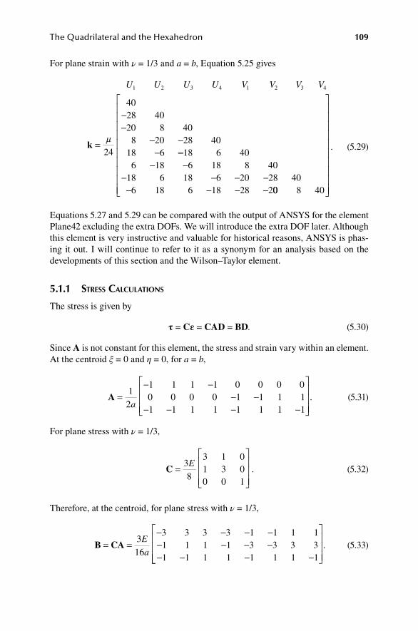
The Quadrilateral and the Hexahedron 109
For plane strain with ν = 1/3 and a = b, Equation 5.25 gives
U U U U V V V V1 2 3 4 1 2 3 4
24
4028 4020 8 40
8 20 28 4018 6
k =
−−
− −−
µ−−
− −− − − −
− − − −
18 6 406 18 6 18 8 40
18 6 18 6 20 28 406 18 6 18 28 200 8 40
. (5.29)
Equations 5.27 and 5.29 can be compared with the output of ANSYS for the element Plane42 excluding the extra DOFs. We will introduce the extra DOF later. Although this element is very instructive and valuable for historical reasons, ANSYS is phas-ing it out. I will continue to refer to it as a synonym for an analysis based on the developments of this section and the Wilson–Taylor element.
5.1.1 StreSS calculationS
The stress is given by
τ = Cε = CAD = BD. (5.30)
Since A is not constant for this element, the stress and strain vary within an element. At the centroid ξ = 0 and η = 0, for a = b,
A =− −
− −− − − −
12
1 1 1 1 0 0 0 00 0 0 0 1 1 1 11 1 1 1 1 1 1 1
a. (5.31)
For plane stress with ν = 1/3,
C =
38
3 1 01 3 00 0 1
E.
(5.32)
Therefore, at the centroid, for plane stress with ν = 1/3,
B CA= =− − − −− − − −− − − −
316
3 3 3 3 1 1 1 11 1 1 1 3 3 3 31 1 1 1 1 1 1 1
E
a
.
(5.33)

110 The Finite Element Method for Mechanics of Solids with ANSYS Applications
For node 3, ξ = 1 and η = 1. For a = b,
A =−
−− −
10 0 1 1 0 0 0 00 0 0 0 0 1 1 00 1 1 0 0 0 1 1
a. (5.34)
Therefore, at node 3, for plane stress with ν = 1/3,
B =− −− −
− −
38
0 0 3 3 0 1 1 00 0 1 1 0 3 3 00 1 1 0 0 0 1 1
E
a. (5.35)
For the Plane42 element, by default, ANSYS provides the stress evaluated at the nodes in the element listing and the stress at the centroid in the Element Table (ETABLE). Stress at the integration points (IPs), which will be defined below, is available in the element listing and the nodal stress listing if ERESX = No, Solution > Load Step Options > Output Ctrls > Integration Point. The IP stresses are then copied to the nodal points, while the element table still has the stress at the centroid.
For the Plane182 element, by default, ANSYS provides the stress evaluated at the nodes in the element listing. Stress at the IP is available in the element listing and the nodal stress listing if ERESX = No; the IP stresses are then copied to the nodal points. There is no ETABLE for stress.
The components of stress are generally not continuous across element boundaries, so the value at a node may be different for all elements sharing that node. The stress at the node as reported by ANSYS is the average of values for all elements sharing the node.
5.1.2 plane StreSS exaMple: pure Bending
The support conditions (Figure 5.2) are zero displacement of the origin and v(a,0) = 0. There is symmetry (S: u = 0, τxy = 0) about the centerline (x = a/2) and antisym-metry (A: u = 0, τyy = 0) about the x axis, so we need only analyze one-quarter of the
p
p p
p
b
a
yx
fIgure 5.2 Pure bending.

The Quadrilateral and the Hexahedron 111
region with zero displacement at the origin (Figure 5.3). The region can be divided into square elements by N divisions on an edge to produce N 2 elements and (N + 1)2 nodes. For a = b = 2, p = 1, E = 1, ν = 0.3, the solution is shown in Table 5.1.
In this case, the actual distribution of displacement is close to that of the shape functions so relatively few elements are needed for a close answer. Let us investigate the case N = 2, shown in Figure 5.4 in more detail. From 5.14, we see that the stress components will vary linearly in y when x is constant. The element output for ele-ment 2 is τxx = 0.51426 at node 5. The element output for element 4 is τxx = 0.46632 at node 5. The stress tensor is not continuous between elements and the data have to be smoothed in some fashion in order to obtain a reasonable estimate of the stress at the element boundary. ANSYS does that by averaging the values from all ele-ments connected to a node. The reported stress at node 5 is therefore τxx = (0.51426 + 0.46632)/2 = 0.49029.
b/2
a/2
p
yx A
S
fIgure 5.3 Bending with symmetry.
taBle 5.1nodal values
N v(1,0) τxx(1,1)
1 0.44608 0.93627
2 0.48528 0.98985
4 0.49643 1.0039
8 0.49911 1.0041
16 0.49978 1.0026
32 0.49994 1.0014
64 0.49999 1.0007
Exact 0.5 1
22
31
1
83
6 7 44
9 5
yx
fIgure 5.4 A 2 × 2 element layout.

112 The Finite Element Method for Mechanics of Solids with ANSYS Applications
5.1.3 plane Strain exaMple: Bending with Shear
The exact solution for the plane strain of a rectangular region loaded by parabolic shear stress on one end (Figure 5.5) is given in Section 2.1.12. We will now apply the finite element method (FEM) using the four-node element to obtain an approximate solution for the case c = 2, L = 16, P = 32, E = 8192, ν = 0.3. Symmetry about the x axis can be used. The mesh chosen has N divisions along the y axis and M divisions along the x axis. A 4 × 8 mesh for the upper half is shown (Figure 5.6). The coordi-nate axes have been shifted for computational convenience.
The edge y = 0 has ux = 0 by symmetry. To prevent rigid body motion, we will fix the origin and set ux = 0 at the upper left corner (x = 0, y = c). The exact solution for the vertical displacement at the center of the right edge is
uPL
Ec
c
Ly = − + +
−
3 2
3
2
2
1
21
42 1
( ) ( )( )
ν νν
.
(5.36)
Table 5.2 shows the FEM solution obtained from ANSYS using the Plane42 ele-ment without extra DOF. From 5.36, the exact displacement is 0.9537 for ν = 0.3 and 0.8037 for ν = 0.499. Note the relatively poor solution for the Poisson ratio near 0.5 when the bulk modulus is very large compared to the shear modulus.
5.1.4 plane StreSS exaMple: Short BeaM
The same plane stress problem that was analyzed in Section 4.4 using constant strain triangles will be analyzed by using the four-node rectangular elements. The strains, and therefore the stresses, vary linearly within each element in this case. The finite element layout is shown in Figure 5.7. There are N segments per side, N 2 rectangles,
σx
τxy τxy
2c
L
fIgure 5.5 Plane strain bending with shear.
σ = 96y
y
x
τ = 12 – 3y2 τ = 12 – 3y2
fIgure 5.6 Bending with shear: element layout.

The Quadrilateral and the Hexahedron 113
and (N + 1)2 nodes. The nodes along the bottom have zero displacement and the nodes along the top have generalized forces as shown.
The displacement of the corner is listed in Table 5.3 for several mesh sizes, for ν = 1/3. The stress distribution for the case of 2500 rectangles is presented in Figures 5.8 through 5.10. The element stress is calculated at the centroid of the element using 5.33.
taBle 5.2displacements for different poisson ratio
N × M ν uy feM/exact
4 × 8 0.3 0.847 0.888
8 × 32 0.3 0.940 0.986
16 × 64 0.3 0.950 0.996
4 × 8 0.499 0.264 0.328
8 × 32 0.499 0.529 0.658
16 × 64 0.499 0.703 0.875
1/8 1/81/4 1/4 1/4
fIgure 5.7 Short beam: element layout.
taBle 5.3convergence
Segments per Side no. of nodes no. of rectangles x displacement of the corner
1 4 1 4.667
2 9 4 5.908
4 25 16 6.792
10 121 100 7.240
20 441 400 7.355
46 2,209 2,216 7.409
50 2,601 2,500 7.412
60 3,721 3,600 7.417
70 5,041 4,900 7.421
80 6,561 6,400 7.424
90 8,281 8,100 7.426
100 1,020 10,000 7.428
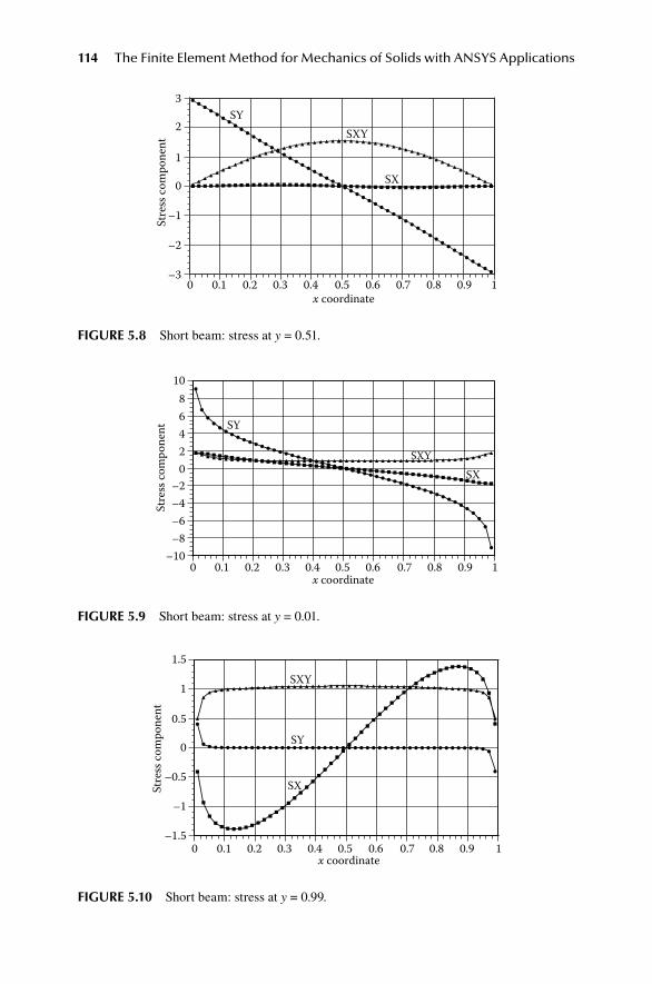
114 The Finite Element Method for Mechanics of Solids with ANSYS Applications
3
2
1
0
–1
–2
–30 0.2 0.4 0.5 0.6 0.7 0.8 0.9 10.1 0.3
x coordinate
Stre
ss c
ompo
nent
SY
SX
SXY
fIgure 5.8 Short beam: stress at y = 0.51.
0 0.1 0.2 0.3 0.4 0.5 0.6 0.7 0.8 0.9 1x coordinate
Stre
ss c
ompo
nent
1086420
–2–4–6–8
–10
SY
SXY
SX
fIgure 5.9 Short beam: stress at y = 0.01.
0
Stre
ss c
ompo
nent
1.5
1
0.5
0
–0.5
–1
–1.50.1 0.2 0.3 0.4 0.5
x coordinate0.6 0.7 0.8 0.9 1
SX
SY
SXY
fIgure 5.10 Short beam: stress at y = 0.99.
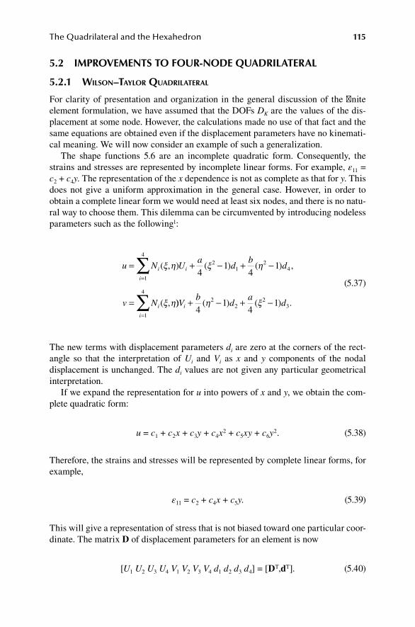
The Quadrilateral and the Hexahedron 115
5.2 IMproveMentS to four-node quadrIlateral
5.2.1 wilSon–taylor quadrilateral
For clarity of presentation and organization in the general discussion of the finite element formulation, we have assumed that the DOFs DK are the values of the dis-placement at some node. However, the calculations made no use of that fact and the same equations are obtained even if the displacement parameters have no kinemati-cal meaning. We will now consider an example of such a generalization.
The shape functions 5.6 are an incomplete quadratic form. Consequently, the strains and stresses are represented by incomplete linear forms. For example, ε11 = c2 + c4y. The representation of the x dependence is not as complete as that for y. This does not give a uniform approximation in the general case. However, in order to obtain a complete linear form we would need at least six nodes, and there is no natu-ral way to choose them. This dilemma can be circumvented by introducing nodeless parameters such as the following1:
u N Ua
db
d
v N
i i
i
i
= + − + −
=
=∑ ( , ) ( ) ( ) ,
( ,
ξ η ξ η
ξ η
1
42
12
441
41
)) ( ) ( ) .Vb
da
di
i=∑ + − + −
1
42
22
341
41η ξ
(5.37)
The new terms with displacement parameters di are zero at the corners of the rect-angle so that the interpretation of Ui and Vi as x and y components of the nodal displacement is unchanged. The di values are not given any particular geometrical interpretation.
If we expand the representation for u into powers of x and y, we obtain the com-plete quadratic form:
u = c1 + c2x + c3y + c4x2 + c5xy + c6y2. (5.38)
Therefore, the strains and stresses will be represented by complete linear forms, for example,
ε11 = c2 + c4x + c5y. (5.39)
This will give a representation of stress that is not biased toward one particular coor-dinate. The matrix D of displacement parameters for an element is now
[U1 U2 U3 U4 V1 V2 V3 V4 d1 d2 d3 d4] = [DT,dT]. (5.40)
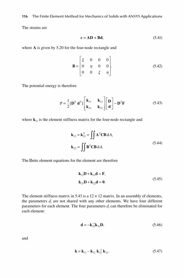
116 The Finite Element Method for Mechanics of Solids with ANSYS Applications
The strains are
ε = AD + Bd, (5.41)
where A is given by 5.20 for the four-node rectangle and
B =
ξ
ηξ η
0 0 0
0 0 0
0 0
.
(5.42)
The potential energy is therefore
P =
−1
211 12
21 22
[ ]D dk k
k kDd
D FT T T
(5.43)
where k11 is the element stiffness matrix for the four-node rectangle and
k k A CB
k B CB
12 21
22
= =
=
∫∫∫∫
T T
T
d
d
A
A
,
.
(5.44)
The finite element equations for the element are therefore
k D k d F
k D k d 0
11 12
21 22
+ =
+ =
,
. (5.45)
The element stiffness matrix in 5.43 is a 12 × 12 matrix. In an assembly of elements, the parameters di are not shared with any other elements. We have four different parameters for each element. The four parameters di can therefore be eliminated for each element:
d k k D= − −221
21 , (5.46)
and
k k k k k= − −11 12 22
121. (5.47)

The Quadrilateral and the Hexahedron 117
This process is called static condensation. The result 5.47 is an 8 × 8 element stiff-ness matrix that may be used in place of the four-node serendipity element. This new matrix will give improved displacements and stresses for a given number of rect-angles. The results for the short beam example are shown in Figure 5.11. The results are significantly improved for a small number of elements, and the result appears to converge to the same result as for the four-node rectangles.
For a = b and ν = 1/3, the first row is
U U U U V V V V
k i
1 2 3 4 1 2 3 4
1 3654 36 36 18 27 9 27 9[ ] = − − − −
µpplane strain.
p[ ] k i1 3644 26 28 10 18 0 18 0= − − −
µllane stress.
(5.48)
This agrees with ANSYS element Plane42 with extra DOFs.If we investigate the displacement field for an assembly of nonrectangular ele-
ments, we find that representation 5.37 does not generate a continuous displacement field. Because of the ξ2 and η2 terms, the displacement is not varying linearly along a side unless di = 0. This violates the assumptions in the derivation of the finite element equations from the potential energy.
Elements that do not generate continuous displacement fields when they are assembled are called incompatible or nonconforming. We will see later that this particular nonconforming element is acceptable as long as the element is rectan-gular, or the corresponding isoparametric element is a parallelogram. A modified integration scheme has been invented that removes the restriction to parallelograms.2
Disp
lace
men
t
Number of segments1
8
7
6
5
46 11 16 21
without extra DOFswith extra DOFs
fIgure 5.11 Comparison with extra DOF.

118 The Finite Element Method for Mechanics of Solids with ANSYS Applications
It is presented in Section 6.3.1. The Wilson–Taylor element is a special case of the following enhanced strain element.
5.2.2 enhanced Strain forMulation
A potential energy function for the Wilson–Taylor element can be established by regarding the extra strain resulting from the nodeless parameters as an independent variable that is not derived from the displacements.3 Let us consider the modified potential energy function
P AV V
( , , ) ( )u ττ εε εε εε= + −( ) − −∫ ∫τ εij ij i i i iV b u V T ud d 0 ddA
TS∫ , (5.49)
where ε is derived from u by the strain–displacement relations and εε is a parameter called the enhanced strain tensor. Continuity is required for the displacement u but not for the stress τ nor the enhanced strain εε. If εε = 0, 5.49 reduces to the potential energy formula. For linear elasticity,
A( )εε εε+ = +( ) +( )
12
cijkm ij ij km kmε εε ε , (5.50)
with cijkm = cjikm = cijmk = ckmij. The derivative of P is
δ δε ε τ ε ε δτPV V
= +( ) − −∫ c V Vijkm km km ij ij ij ij d d∫∫
∫ ∫+ +( ) − −c V b u V T uijkm km km ij i i i iε ε εδ δ δ d dV V
0 ddA
TS∫ .
(5.51)
Integrating by parts, subject to the condition that u is as continuous function and δu = 0 on Su,
D c V Vijkm km km ij ij ij ijPV V
= +( ) − −∫ ε ε τ ε ε τδ δ d d∫∫
∫− +( )( ) +
+
c b u V
n c
ijkm km km j i i
j ijkm km
ε ε
ε
δ , dV
++( ) − ∫ ε δkm i iT u A
T
0 dS
.
(5.52)

The Quadrilateral and the Hexahedron 119
Thus, DP = 0 is equivalent to
ε
τ ε ε
τ
ij
ij ijkm km km
ij j i
c
b
=
= +( )+ =
0
0
,
,
, ,
(5.53)
in V, and
n Tj ij iτ = 0
(5.54)
on ST. These are the equations of linear elasticity.We can now apply FEM to formulate a solution procedure. In matrix form, using
5.51, DP = 0 gives
δ
δ
δ
εε εε εε ττ
ττ εε
εε εε εε
T
T
T
d
d
C C
C C
+ − =
=
+
∫
∫
V
V
V
V
0
0
,
,
= +∫ ∫ ∫d d dT TV V A
TV V S
δ δu b u T .
(5.55)
We introduce shape functions for the three fields:
u ND AD S Gd= = =, , , .εε ττ σσ εε == (5.56)
Both d and σ are nodeless parameters for each element and are not shared by other elements. Matrix A is determined by N through the strain–displacement relations. Substituting into 5.55 and merging the element equations, we find from the second equation that
S G dT d .VV∫ = 0
(5.57)
Therefore, we will require that the shape functions are such that
S GT dVV∫ = 0.
(5.58)
The first and third equations in 5.55 then reduce to
k11D + k12d = F, (5.59)

120 The Finite Element Method for Mechanics of Solids with ANSYS Applications
and
k21D + k22d = 0, (5.60)
where
k A
k k G
k G
11
12 21
22
=
= =
=
∫
∫
∫
T
T T
T
d
d
d
CA
CA
CG
V
V
V
V
V
V
,
,
.
(5.61)
The force matrix is the same as for the pure displacement formulation and is not affected by the introduction of the enhanced strain. Since the parameters d are not shared by elements, they can be eliminated at the element level by static condensation:
d k k D= − −221
21 , (5.62)
to obtain the element stiffness matrix
k k k k k= − −11 12 22
121. (5.63)
Wilson–Taylor Element. Let us now treat the plane problem using the four-node element with nodeless parameters and treat the nodeless parameters as generating the enhanced strain:
G =
ξ
ηξ η
0 0 0
0 0 0
0 0
.
(5.64)
In order to satisfy 5.58, we can chose
S =
1 0 0 0
0 1 0 0
0 0 1 0 0
ηξ .
(5.65)
For plane strain with ν = 1/3,
C =
µ4 2 02 4 00 0 1
.
(5.66)

The Quadrilateral and the Hexahedron 121
For a square element,
k22 3
4 0 0 00 4 0 00 0 1 00 0 0 1
=
abµ,
(5.67)
and
k21 6
0 2 0 2 0 2 0 22 0 2 0 2 0 2 01 0 1 0 1 0 1 00 1 0 1 0 1 0 1
=
− −− −− −
− −
µa
.
(5.68)
Therefore,
U V U V U V U V1 1 2 2 3 3 4 4
12 221
21 6
10 11 0 10 1 0 11 0 1 0
k k k− =
−−
−µ
110 1 0 1 0 11 0 1 0 1 0 10 1 0 1 0 1 0 1
−− −
− −
. (5.69)
Combined with 5.27, we find that the element stiffness matrix for plane strain is
U U U U V V V V1 2 3 4 1 2 3 4
24
3624 3624 12 3612 24 24 3618
k =
−−
− −µ−− −
− −− − − −
− − −
6 18 6 366 18 6 8 12 36
18 6 18 6 24 24 366 18 6 18 24 −−
24 12 36
. (5.70)
This is the same as for ANSYS Plane42 element with extra DOF and the ANSYS Plane182 element with enhanced strain.

122 The Finite Element Method for Mechanics of Solids with ANSYS Applications
5.2.3 approxiMate VoluMetric StrainS
We see from Table 5.2 that the solution when the Poisson ration is near 0.5 is poor for any mesh. The basic serendipity element is apparently giving too much weight to the volume change relative to the distortion because of the large bulk modulus, that is, the element is too stiff in volume change. The performance can be improved by using a lower-order integration on the volumetric terms. We will explore that option in this and the next two sections.
For the plane problem γxz = γyz = 0 and
σ
σ
τ
σ
ε
ε
γ
ε
x
y
xy
z
x
y
xy
z
=
C
(5.71)
where
C =
++
+
2 0
2 0
0 0 0
0 2
µ λ λ λλ µ λ λ
µλ λ µ λ
(5.72)
and
ε νν
ε εz
x y
=−
−+( )
0 for plane strain.
1for plane stresss.
(5.73)
The total strains can be expressed in terms of the deviatoric strains and the volumet-ric strain
ε
ε
γ
ε
γ
x
y
xy
z
x
y
xy
z
e
e
e
=
++
13 0
ε
ε
ε
v
v
v
.
(5.74)
From 5.19,
εx = A1U, εy = A2V, γxy = A2U + A1V. (5.75)

The Quadrilateral and the Hexahedron 123
For plane strain,
ε ε εv x y= + =
A A U
V1 2 .
(5.76)
Therefore, for plane strain,
e
e
e
x
y
xy
z
γ
=
A 0
0 A
A A
0 0
1
2
2 1
−
UV
A A
A A
0 0A A
UV
13
1 2
1 2
1 2
=
−
−
− −
23
13
13
23
13
13
A B
A B
B A
A B
UV
.
(5.77)
Define
A
A A
A A
0 0A A
( )dil =
13
1 2
1 2
1 2
(5.78)
and
A
A A
A A
A A
A A
( )dev =
−
−
− −
23
13
13
23
13
13
1 2
1 2
2 1
1 2
. (5.79)
Thus,
ε
ε
γ
ε
x
y
xy
z
=
+A U
VA U
V( ) ( )dev dil
. (5.80)
We now approximate the dilatational term by evaluating matrix A(dil) at the centroid (ξ = η = 0) of the element. This procedure is known as the B method.4 Then,
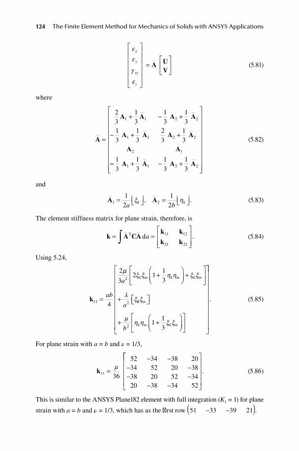
124 The Finite Element Method for Mechanics of Solids with ANSYS Applications
ε
ε
γ
ε
x
y
xy
z
=
A U
V
(5.81)
where
A
A A A A
A A A A
A A=
+ − +
− + +
23
13
13
13
13
13
23
13
1 1 2 2
1 1 2 2
2 1
−− + − +
13
13
13
131 1 2 2A A A A
(5.82)
and
A A1 2
12
12
= = a bk kξ η, .
(5.83)
The element stiffness matrix for plane strain, therefore, is
k A CAk k
k k= =
∫ T da 11 12
21 22
. (5.84)
Using 5.24,
k11
2
24
2
32 1
13
=
+
+
+ab
a
a
k m k m k m
µξ ξ η η ξ ξ
λξkk m
k m k mb
ξ
µη η ξ ξ
+ +
2
113
. (5.85)
For plane strain with a = b and ν = 1/3,
k11 36
52 34 38 2034 52 20 3838 20 52 3420 38 34 52
=
− −− −− −
− −
µ
. (5.86)
This is similar to the ANSYS Plane182 element with full integration (K1 = 1) for plane
strain with a = b and ν = 1/3, which has as the first row 51 33 39 21− −( ).
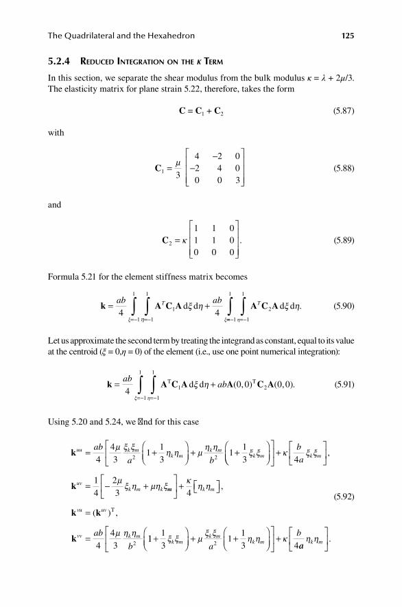
The Quadrilateral and the Hexahedron 125
5.2.4 reduced integration on the k terM
In this section, we separate the shear modulus from the bulk modulus κ = λ + 2μ/3. The elasticity matrix for plane strain 5.22, therefore, takes the form
C = C1 + C2 (5.87)
with
C1 3
4 2 02 4 00 0 3
=−
−
µ
(5.88)
and
C2
1 1 01 1 00 0 0
=
κ . (5.89)
Formula 5.21 for the element stiffness matrix becomes
k A C A A C A= +=−=− =−∫∫ ∫ab abT T
4 41
1
1
1
1
2
1
1
d d d dξ η ξ ηηξ ηξ
.==−∫
1
1
(5.90)
Let us approximate the second term by treating the integrand as constant, equal to its value at the centroid (ξ = 0,η = 0) of the element (i.e., use one point numerical integration):
k A C A A C A= +=−=−∫∫ab
ab4
0 0 0 01 2
1
1
1
1
T Td dξ ηηξ
( , ) ( , ).
(5.91)
Using 5.20 and 5.24, we find for this case
kuu k mk m
k mk m
ab
a b= +
+ +
443
113
1132 2
µ ξ ξη η µ
η ηξ ξ
+
= − +
κ ξ ξ
µξ η µη ξ
b
a k m
uvk m k
4
14
23
,
k mm k m
vu uv
vv k mab
b
+
=
=
κη η
µ η η
4
443 2
,
( ) ,k k
k
T
1113
113 42
+
+ +
+ξ ξ µ
ξ ξη η κk m
k mk m
a
b
aa k mη η
.
(5.92)

126 The Finite Element Method for Mechanics of Solids with ANSYS Applications
For a = b and ν = 1/3,
U U U U V V V V
k i
1 2 3 4 1 2 3 4
1 3652 34 38 20 27 9 27 9[ ] = − − − −
µ
(5.93)
in agreement with 5.86.
5.2.5 reduced integration on the λ terM
In this section, we separate the dependence on μ and λ = 2μν/(1 – 2ν) since λ is large for ν near 0.5. For plane strain,
C = C1 + C2, (5.94)
where
C1
2 0 00 2 00 0 1
=
µ
(5.95)
and
C2
1 1 01 1 00 0 0
=
λ .
(5.96)
Formula 5.21 for the element stiffness matrix then becomes
k A C A A C A= +=−=− =−=∫∫ ∫ab ab
4 41
1
1
1
1
2
1
1
T Td d d dξ η ξ ηηξ ηξ −−
∫1
1
.
(5.97)
Let us approximate the second term by treating the integrand as constant, equal to its value at the centroid (ξ = 0,η = 0) of the element (i.e., use one-point numerical integration):
k A C A A C A= +=−=−∫∫ab
ab4
0 0 0 01 2
1
1
1
1
T Td dξ ηηξ
( , ) ( , ).
(5.98)

The Quadrilateral and the Hexahedron 127
Using 5.20, 5.95, and 5.96,
kA A A A A A
A A A A A A=
+
+
ab
4
2
2
1 1 2 2 2 1
1 2 2 2 1 1
µT T T
T T T
+
=−=−∫∫ d d
T T
ξ η
λ
ηξ 1
1
1
1
1 1 1 2
2
0 0 0 0ab
A A A A
A
( ) ( ) ( ) ( )
(00 0 0 01 2 2) ( ) ( ) ( ).
T TA A A
(5.99)
For a square element with ν = 1/3, λ = 2μ, for plane strain,
U U U U V V V V1 2 3 4 1 2 3 4
8
12 8 8 4 6 2 6 28 12 4 8 2 6 2 6
k =
− − − −− − − −−
µ88 4 12 8 6 2 6 24 8 8 12 2 6 2 66 2 6 2 12 4 8 82 6 2 6 4 1
− − −− − − −− − − −− − 22 8 8
6 2 6 2 8 8 12 42 6 2 6 8 8 4 12
− −− − − −− − − −
. (5.100)
This matrix agrees with the enhanced strain matrix 5.70.
5.2.6 uniforM reduced integration
Since the reduced integration of the λ terms results in such significant improvement, especially for a Poisson ratio near 0.5, one is tempted to try a reduced integration on both integrals. In such a case, formula 5.21 for the element stiffness matrix simplifies to
U V
k A CA k kk k
= =
abuu uv
vu vv( , ) ( , )0 0 0 0T .
(5.101)
From 5.14, 5.20, and 5.22, for an isotropic material,
k Cb
aC
a
b
k C
kmuu
k m k m
kmuv
k
= +
=
14
14
11 33
12
ξ ξ η η
ξ
,
ηη η ξ
η η
m k m
kmvu
mkuv
kmvv
k m
C
k k
k Ca
bC
+
=
= +
33
22
14
,
,
333
b
a k mξ ξ
.
(5.102)
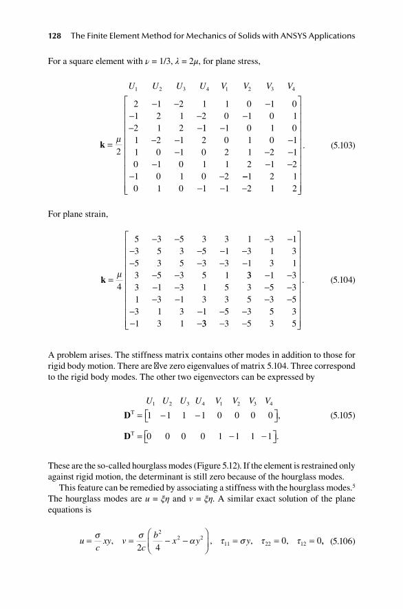
128 The Finite Element Method for Mechanics of Solids with ANSYS Applications
For a square element with ν = 1/3, λ = 2μ, for plane stress,
U U U U V V V V1 2 3 4 1 2 3 4
2
2 1 1 01 2 1 2 0 1 0 12 1 2
k =
− − −− − −− −
µ
2 1 1 0
11 1 0 1 02 1 2 0 1 0 10 1 0 2 1 2 11 0 1 1 2 1 2
1 0 1 0 2
−− − −
− − −− − −
− −
110
−−− − −
1 2 11 1 2 1 20 1 0
. (5.103)
For plane strain,
k =
− − − −− − − −− − − −
− −µ4
5 3 5 3 3 3 13 5 3 5 1 3 1 35 3 5 3 3 1 3 1
5 3 5 1
1
3 33 1 31 3 1 5 3 5 33 1 3 3 5 3 5
3 1 3 1 5 3 5 31 3 1
− −− − − −− − − −
− − − −− −
31
33 3 5 3 5− −
. (5.104)
A problem arises. The stiffness matrix contains other modes in addition to those for rigid body motion. There are five zero eigenvalues of matrix 5.104. Three correspond to the rigid body modes. The other two eigenvectors can be expressed by
U U U U V V V V1 2 3 4 1 2 3 4
1 1 1 1 0TD = − − 0 0 0
0 0 0 0T
=
,
D 1 1 1 1− − .
(5.105)
These are the so-called hourglass modes (Figure 5.12). If the element is restrained only against rigid motion, the determinant is still zero because of the hourglass modes.
This feature can be remedied by associating a stiffness with the hourglass modes.5 The hourglass modes are u = ξη and v = ξη. A similar exact solution of the plane equations is
uc
xy vc
bx y y= = − −
= = =σ σ
α τ σ τ τ, , , ,2 4
0 02
2 211 22 12 ,,
(5.106)
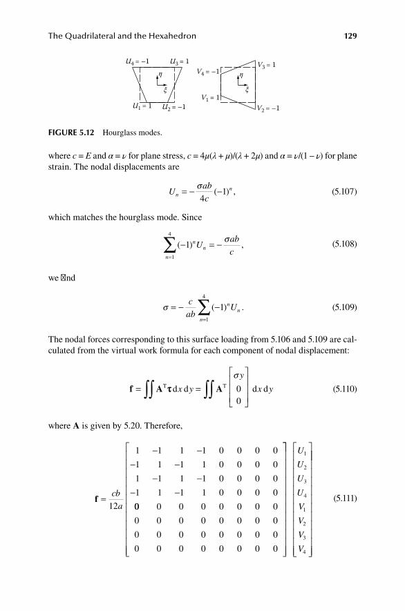
The Quadrilateral and the Hexahedron 129
where c = E and α = ν for plane stress, c = 4μ(λ + μ)/(λ + 2μ) and α = ν/(1 – ν) for plane strain. The nodal displacements are
U
ab
cnn= − −σ
41( ) ,
(5.107)
which matches the hourglass mode. Since
( )− = −=
∑ 11
4n
n
n
Uab
c
σ,
(5.108)
we find
σ = − −=
∑c
abUn
n
n
( )11
4
.
(5.109)
The nodal forces corresponding to this surface loading from 5.106 and 5.109 are cal-culated from the virtual work formula for each component of nodal displacement:
f A A= =
∫∫ ∫∫T Td d d dττ x y
y
x y
σ
00
(5.110)
where A is given by 5.20. Therefore,
f =
− −− −
− −− −cb
a12
1 1 1 1 0 0 0 0
1 1 1 1 0 0 0 0
1 1 1 1 0 0 0 0
1 1 1 1 0 0 0 0
00 0 0 0 0 0 0 0
0 0 0 0 0 0 0 0
0 0 0 0 0 0 0 0
0 0 0 0 0 0 0 0
U
U
U
U
V
V
V
V
1
2
3
4
1
2
3
4
(5.111)
U4 = –1
U1 = 1 U2 = –1
U3 = 1 V3 = 1
V2 = –1V1 = 1
V4 = –1ƞ ƞ
ξ ξ
fIgure 5.12 Hourglass modes.

130 The Finite Element Method for Mechanics of Solids with ANSYS Applications
for the first hourglass mode. For the second mode,
f =−
cb
a12
0 0 0 0 0 0 0 0
0 0 0 0 0 0 0 0
0 0 0 0 0 0 0 0
0 0 0 0 0 0 0 0
0 0 0 0 1 1 1 −−− −
− −− −
1
0 0 0 0 1 1 1 1
0 0 0 0 1 1 1 1
0 0 0 0 1 1 1 1
U
U
U
U
V
V
V
V
1
2
3
4
1
2
3
4
. (5.112)
Adding the results for the two modes, we find the associated hourglass stiffness
k =
− −− −
− −− −cb
a12
1 1 1 1 0 0 0 01 1 1 1 0 0 0 01 1 1 1 0 0 0 01 1 1 1 0 0 0 000 0 0 0 1 1 1 10 0 0 0 1 1 1 10 0 0 0 1 1 1 10 0 0 0 1 1 1 1
− −− −
− −− −
. (5.113)
A very small fraction of this stiffness is added to the singular element stiffness 5.103 to stabilize the hourglass modes without contributing significantly to the calculated displacements. ANSYS allows control of this factor by the parameter HGSTF. If the entire hourglass correction is added back, the stiffness matrix agrees with matrix 5.100 obtained by reduced integration on the λ terms. If the element is not rectangu-lar, the definition of the hourglass modes must be altered.6
5.2.7 exaMple uSing iMproVed eleMentS
The plane strain problem illustrated in Section 5.1.3 is analyzed using a 16 × 64 mesh using the Plane182 element of ANSYS. The result is shown in Table 5.4. This shows considerable improvement over the basic element as shown in Table 5.2 for ν near 0.5.
5.3 nuMerIcal IntegratIon
Evaluation of the stiffness matrix involves integration over the region. This can be complicated for an arbitrary shape. It is therefore common to use numerical integra-tion to obtain an approximate evaluation of the area and volume integrals.

The Quadrilateral and the Hexahedron 131
In order to evaluate the integral
f x xa
b
( ) d∫ , (5.114)
we choose several points xi within the interval (a, b) and let f(xk) be denoted by fk (Figure 5.13). We can approximate f(x) in terms of the intermediate values fk by some convenient curve fitting technique that makes integration easy. Then,
f x x W fa
b
n n
n
N
( ) .d∫ ∑==1
(5.115)
The numerical coefficients Wn have been tabulated in reference works on numerical analysis for various choices of points xk and interpolation functions. For multiple integrals, proceed by iterated integrals:
f x y x y f X y W y
W W f
a
b
c
d
n n
n
N
c
d
n
m
N
m
( , ) ( , )d d d∫∫ ∑∫
∑
=
=
=
=
1
1
(( , ).X Yn m
n
N
=∑
1
(5.116)
taBle 5.4comparison of Integration Methods
element option ν uy feM/exact
Full Integration (B) 0.3 0.951 0.997
Enhanced Strain 0.3 0.952 0.998
Reduced Integration 0.3 0.954 1.000
Full Integration (B) 0.499 0.802 0.998
Enhanced Strain 0.499 0.802 0.998
Reduced Integration 0.499 0.804 1.000
xa bx1
f1f2
f3
x2 x3
f(x)
fIgure 5.13 Numerical integration.

132 The Finite Element Method for Mechanics of Solids with ANSYS Applications
The most commonly used method of numerical integration for finite element applica-tions is Gauss quadratures. In this method, the points xn and coefficients Wn are cho-sen so that an exact result is obtained when f(x) is a polynomial equal to 1, x, x2, …, x2N−l. This gives 2N conditions with which to determine the 2N quantities Wn and xn.
For example, consider the case N = 2 and –1 ≤ x ≤ 1:
c c x c x c x x W f x W f x1 2 32
43
1
1
1 1 2 2+ + +( ) ≡ +−∫ d ( ) ( ).
(5.117)
From which,
2
231 3 1 1 2 1 3 1
24 1
32 1 2 2 3 2c c W c c x c x c x W c c x c x+ ≡ + + +( ) + + + 22
4 23+( )c x . (5.118)
It follows that
W W x x1 2 1 21
1
3
1
3= = = − = +, , .
(5.119)
For any function, we have the approximate formula:
f x x W f x W f x f f( ) ( ) ( ) ( . ) ( . ).d−∫ = + = − + +1
1
1 1 2 2 0 577 0 577
(5.120)
The factors have been tabulated7 for a large number of choices of N. The results for one-, two-, three-, and four-point approximations for a = −1 and b = +1 are shown in Table 5.5. Note that the one-point integration is equivalent to taking the integrand as a constant equal to its value at the centroid.
taBle 5.5Weighting factors
N = 1 X1 = 0 W1 = 2
N = 2 X1 = −0.57735027 W1 = 1
X2 = +0.57735027 W2 = 1
N = 3 X1 = −0.77459 W1 = 0.55555
X2 = 0 W2 = 0.88888
X3 = +0.77459 W3 = 0.55555
N = 4 X1 = −0.86113 W1 = 0.34785
X2 = −0.33998 W2 = 0.65214
X3 = +0.33998 W3 = 0.65214
X4 = +0.86113 W4 = 0.34785

The Quadrilateral and the Hexahedron 133
5.4 coordInate tranSforMatIonS
To extend the previous results for rectangles, we need to introduce local coordinates for the element that are appropriate to the actual shape of the element. We gather here the formulas for transformation from the global rectangular Cartesian coordinates to local coordinates.
Consider a plane region covered by a rectangular Cartesian coordinate system (x,y) = (x1,x2). Let us introduce a new (curvilinear) coordinate system by expressing xα in terms of new parameters (ξ,η) ≡ (ξ1,ξ2) by xα = xα(ξ1,ξ2). We always choose a transformation that can be inverted: ξα = ξα(x1, x2). Let
∂∂x
Jα
βαβξ
= ,
(5.121)
and keep in mind that Jαβ is a function of (ξ,η). Furthermore, let
∂∂
ξα
βαβx
J= * .
(5.122)
We then have (the summation convention applies to repeated indices):
∂∂
∂∂
∂∂
x
x
x
xα
φ
φ
β
α
βαβξ
ξδ= = .
(5.123)
Thus,
J Jαφ φβ αβδ* .=
(5.124)
In matrix notation
JJ* = 1. (5.125)
The coordinate transformation is required to be invertible and therefore the determi-nant of J is nonzero:
J = det J ≠ 0. (5.126)
Integration over a region of the plane can be expressed in terms of the rectangular Cartesian system or the curvilinear coordinate system. For the rectangular Cartesian system, da = dxdy. For the curvilinear system, da = Jdξdη. Therefore,
f x y x y f a fJ f
R R R R
( , ) ( , ) .d d d d d d d∫∫ ∫∫ ∫∫ ∫∫= = =ξ η ξ η ξ η
(5.127)

134 The Finite Element Method for Mechanics of Solids with ANSYS Applications
If the coordinate transformation maps the region onto the square –1 ≤ ξ ≤ 1, –1 ≤ η ≤ 1, then integration formula 5.116 can be used:
f W W fR
n
m
N
m n m
n
N
( , ) ( , ).ξ η ξ η ξ ηd d∫∫ ∑∑=== 11
(5.128)
5.5 ISoparaMetrIc quadrIlateral
Consider a general plane quadrilateral (Figure 5.14). Let us introduce a coordinate transformation such that the equation of the boundary segments has the simple form that ξ is constant or η is constant:
x N Xk k
k
α αξ η==
∑ ( , ) ,1
4
(5.129)
where (X1k,X2k) ≡ (Xk,Yk) are the (x,y) coordinates of node k. One such coordinate transformation is determined by the shape functions 5.10. We have, for example, when ξ = +1,
x X X
y Y Y
= − + +
= − + +
12
1 12
1
12
1 12
1
2 3
2 3
( ) ( ) ,
( ) ( ) ,
η η
η η
(5.130)
which is the equation of the line 2–3. We must now find suitable shape functions as for the displacements within the quadrilateral. We will represent the components of dis-placement (u,v) ≡ (u1,v2) in terms of their values (U1k,U2k) ≡ (Uk,Vk) at the four corners:
u N Uk
k
kα αξ η==
∑1
4
( , ) .
(5.131)
ξ1
11
1 2
33
21
44
1
η
η=+1
η=–1
ξ=–1
ξ=+1
ηξ
x
y
fIgure 5.14 General quadrilateral.

The Quadrilateral and the Hexahedron 135
Note that uα and Uαk are components on the (x,y) system, not the (ξ,η) system. In matrix form,
U U U U U U U U
U V U V U V U V
D D D D
11 21 12 22 13 23 14 24
1 1 2 2 3 3 4 4
1 2 3 44 5 6 7 8
1
2
1 2 3 4
1 2 3 4
0 0 0 0
0 0 0 0
D D D D
u
u
N N N N
N N N N
=
D
(5.132)
or
u = ND. (5.133)
This curvilinear coordinate system is the natural choice that will simplify the task of finding suitable shape functions Nk. To achieve a continuous displacement field, it is only necessary to have uα varying linearly with distance along an edge, and
Nk(ξm,ηm) = δkm. (5.134)
Let us investigate the shape functions 5.10. Condition 5.134 is satisfied by this choice. It remains to be determined if the formula for uα is linear along an edge. Along ξ = 1, for example,
u U U
v V V
= − + +
= − + +
12
112
1
12
112
1
2 3
2 3
( ) ( ) ,
( ) ( ) .
η η
η η
(5.135)
We see that u and v do vary linearly along the edge. Similar results hold for the other edges. Therefore, this choice of shape functions will generate a continuous displace-ment field for an assembly of quadrilaterals. When the same functions are used in the coordinate transformation 5.129 and the approximation for displacements 5.131, this procedure is known as the isoparametric formulation.8
We can now proceed to calculate the corresponding element stiffness matrix. From 5.131 and 5.122,
uu
x
u
xN J Uk k
k
α βα
β
α
φ
φ
βφ
φ
φβ αξξ
,* ,≡ = = ∑∑∂
∂∂∂
∂∂
(5.136)

136 The Finite Element Method for Mechanics of Solids with ANSYS Applications
where the derivatives
N
Nk
kα
αξ≡ ∂
∂ (5.137)
are determined from 5.12. From 2.27,
2ε
δ
αβ φ φβ α φ φα β
φ
φ φβ θα
= +
=
∑ N J U N J U
N J
k k k k
k
k
* *
*
,
UU N J U
N J N J
k k k
k
k k
θ φ φα θβ θ
φ θ
φ φβ θα φ φ
δ
δ
+
= +
∑ *
*
, ,
αα θβ θ
φ θ
αβθ θ
θ
δ*
,
, ,
.
=
∑
∑
U
A U
k
k
k k
k
(5.138)
where
A N J N Jk k
k
kαβθ φ φβ θα
φ
φ φα θβδ δ= +∑ ( * * ),
. (5.139)
In matrix form,
U U U U U U U U
U V U V U V U V
D D D D
11 21 12 22 13 23 14 24
1 1 2 2 3 3 4 4
1 2 3 44 5 6 7 8
11
22
12
1111 1121 1112
D D D D
A A Aε
ε
γ
=AA A A A A
A A A A A1122 1113 1123 1114 1124
2211 2221 2212 2222 22213 12223 2214 2224
1211 2111
A A A
A A+
etc.
[ ].Dn
(5.140)
In matrix notation,
ε = AD. (5.141)
By 3.23 and 3.24, the stiffness matrix for the element is
k A CA= ∫ T daR
.
(5.142)

The Quadrilateral and the Hexahedron 137
We need the Jacobian Jαβ = ∂xα/∂ξβ:
Jx x N
X X
J
kk
k
k k k
k
111
1
22
14
1= ∂∂
= ∂∂
= ∂∂
= +
= ∂
∑ ∑ξ ξ ξξ η η( ),
xx y NY Y
J X
kk
k
k k k
k
k
2
2
12
14
1
14
∂= ∂
∂= ∂
∂= +
=
∑ ∑ξ η ηη ξ ξ
η
( ),
kk k
k
k k k
k
J Y
( ),
( ),
1
14
121
+
= +
∑
∑
ξ ξ
ξ η η
(5.143)
where ξk and ηk are nodal coordinates. Thus, Jαβ is a polynomial, but Jαβ* is not, and
the integration is complicated. Numerical integration is therefore used. The integral over the general quadrilateral is accomplished by using the coordinate transforma-tion to (ξ,η) as in 5.127 and using numerical integration as in 5.128.
k f f= =∫∫ ∑∑( , ) ( , )ξ η ξ η ξ ηd d i j i j
ji
W W ,
(5.144)
where ξk and ηk are coordinates of the IPs.The foregoing relations are expressed in the usual matrix form with the follow-
ing correspondence (the numbering is chosen to match the FORTRAN storage convention):
D
D
D
U
V
U
U1
2
3
1
1
2
11
: :
=
= UU
U21
12
:
.
(5.145)
The procedures used in this section to find a stiffness matrix for the quadrilateral as soon as one is known for the rectangle, provide a general method that can be used for other types of elements:
(1) Find the shape functions for the rectangle. (2) Introduce natural coordinates (ξ, η) for the quadrilateral as the inverse of
the coordinate transformation 5.129. (3) Shape functions for the displacements within the quadrilateral are given by
5.131.

138 The Finite Element Method for Mechanics of Solids with ANSYS Applications
(4) Use the general relations to obtain the stiffness matrix for the quadrilateral that involves the integral over the quadrilateral region.
(5) Use numerical integration to evaluate the integral.
5.5.1 wilSon–taylor eleMent
For this element, 5.131 is replaced by
u N U N dk
k
k a a
a
α α αξ η= += =
∑ ∑1
4
1
4
( , ) ext
(5.146)
where
N N
N N
11 212
12 222
1
1
ext ext
ext ext
= = −
= = −
ξ
η
,
.
(5.147)
Equation 5.138 is replaced by
21
4
εαβ αβθ θ
θ
αβ= +∑ ∑=
A U B dk k
k
a a
a.
, (5.148)
where
B
N
x
N
x
NJ
Na
a a a aαβ
α
β
β
α
α
θθ
β
ξ β= ∂∂
+∂
∂= ∂
∂∗ +
∂ext ext ext exxt
∂∗
ξθθαJ . (5.149)
This expression is simplified by evaluating the Jacobean terms Jαβ∗ at the centroid. It
is shown below that the patch test will then be satisfied by the element.
5.5.2 three-node triangle aS a Special caSe of rectangle
The constant strain triangle can be obtained from the four-node quadrilateral as the special case when two nodes coincide (Figure 5.15). Collapsing node 4 onto node 1, the coordinate transformation 5.129 with X1 = X4 and Y1 = Y4 becomes
x X X X
y
= −( ) + +( ) −( ) + +( ) +( )
=
12
114
1 114
1 1
12
1
1 2 3ξ ξ η ξ η ,
−−( ) + +( ) −( ) + +( ) +( )ξ ξ η ξ ηY Y Y1 2 3
14
1 114
1 1 .
(5.150)

The Quadrilateral and the Hexahedron 139
This induces shape functions for the triangle:
N N N1 2 3
12
114
1 114
1 1= −( ) = +( ) −( ) = +( ) +( )ξ ξ η ξ η, , .
(5.151)
Note that
N1 + N2 + N3 = 1. (5.152)
That is, the shape functions satisfy the relation
1 1 1 1
1 2 3
1 2 3
1
2
3
xy
X X X
Y Y Y
N
N
N
=
.
(5.153)
Therefore, by 4.4,
N
N
N
xy
1
2
3
11
2
3
1
=
=
−( )ΦΦ T
ζ
ζ
ζ
(5.154)
where ζi represents the triangular coordinates. These are the shape functions for the constant strain triangle.
5.6 eIght-node quadrIlateral
The shape functions for the four-node rectangle described in Section 5.1 can be extended to an eight-note rectangle in which the additional nodes are placed at the midpoints of the sides, as in Figure 5.16. The natural coordinates (ξ,η) as defined in Section 5.1 will be used here. The formulas for the x and y components of displace-ments in the element have the form
3
2
1
4
3
2
1
xx
yy
fIgure 5.15 Collapse into a triangle.

140 The Finite Element Method for Mechanics of Solids with ANSYS Applications
u N U
v N V
i i
i
i i
i
=
=
=
=
∑
∑
( , ) ,
( , ) .
ξ η
ξ η
1
8
1
8
(5.155)
The shape functions for the corners must be modified so that they are zero at the side nodes, and additional shape functions must be found for the side nodes. Suitable shape functions that can be found by trial and error are as follows.
N i
N
i i i i i
i
= + + + − =
=
14
1 1 1 1 2 3 4( )( )( ), , , , .ξ ξ η η ξ ξ η η
112
1 1 5 7
12
1 1 6 8
2
2
−( ) + =
= + −( ) =
ξ η η
ξ ξ η
( ), , .
( ) , ,
i
i i
i
N i ..
(5.156)
One can see by inspection that the shape functions have the property,
Ni(ξj,ηj) = δij, (5.157)
as required. The continuity between elements now has to be investigated. On the side ξ = 1, for example,
u U U U= − +( ) + +( ) + −( )1
212
122
23
26η η η η η .
(5.158)
That is, u is a quadratic function. Since a quadratic function is uniquely determined by its value at three points, two elements sharing the three nodes on that side will have matching displacements along that side. Similar calculations along the other sides show that continuity between elements is achieved for these shape functions. If one expands the representation for u, the result is of the form
u = c1 + c2ξ + c3η + c4ξ2 + c5ξη + c6η2 + c7ξ2η + c8η2ξ, (5.159)
where coefficients ci are combinations of the nodal values. That is, the representation of u is an incomplete cubic polynomial that utilizes the bold-face terms in Table 5.6.
121 5
34
8 6
7
2
2
2 2 1 1
1η
ξb
b
a a
yx
fIgure 5.16 Eight-node rectangle.

The Quadrilateral and the Hexahedron 141
The important thing is that all of the linear terms are present so that constant strain can be represented exactly. In fact, the displacements are complete in the sec ond-order terms, so that the representation for the strains is complete in the linear terms. The strains for an element are given by
εξ ξ11
1
82 2= ∂
∂= ∂
∂
{ }
=∑a
NU
a
NUk
k
k
kk .
(5.160)
εη η22
1
82 2= ∂
∂= ∂
∂
{ }
=∑b
NV
b
NVk
k
k
kk .
(5.161)
γ
η ξ12
2 2= ∂∂
{ } + ∂
∂
{ }
b
NU
a
NVk
kk
k .
(5.162)
Thus,
U V
A
0
0=
∂∂
∂∂
∂∂
∂
2ab
bN
aN
aN
b
k
k
k
ξ
η
ηNNk
∂
ξ
.
(5.163)
Using 2 × 2 numerical integration, the stiffness matrix of the element is
k A CA f f= = =∫∫ ∫∫−− =
T d d daab ab
i i
i4 4
1
1
1
1
1
( , ) ( , )ξ η ξ η ξ η44
∑
(5.164)
where f = ATCA and ( , ) ( , )ξ ηi i = ± ±1 3 1 3/ / are the coordinates of the IPs. The resulting matrix for a = b and ν = 1/3 is
taBle 5.6polynomial terms
1 ξ ξ2 ξ3
η ξη ξ2η ξ3ηη2 ξη2 ξ2η2 ξ3ηη3 ξη3 ξ2η3 ξ3η3

142 The Finite Element Method for Mechanics of Solids with ANSYS Applications
U V
KK K
K K=
uu uv
uv vvT
(5.165)
where
Kuu =
− − −
209
1 000 0 525 0 500 0 375 1 150 0 350 0 650
µ
. . . . . . . −−− − − −
0 2501 000 0 375 0 500 1 150 0 250 0 650 0 350
1
.. . . . . . .
.. . . . . .. .
000 0 525 0 650 0 250 1 150 0 3501 000 0 650 0
− − − −− − .. . .
. .. .
.
350 1 150 0 2502 600 0 1 000 0
1 400 0 0 200
0 2
− −
−Sym
6600 01 400.
,
(5.166)
K vv =
− − − −
209
1 000 0 375 0 500 0 525 0 250 0 650 0 350
µ
. . . . . . . 11 1501 000 0 525 0 500 0 250 1 150 0 350 0 650
1
.. . . . . . .
.− − − −
0000 0 375 0 350 1 150 0 250 0 6501 000 0 350 0
. . . . .
. . .− − − −− − 6650 0 250 1 150
1 400 0 0 200 02 600 0 1 000
1 40
− −−
. .. .
. .
.
Sym
00 02 600.
,
(5.167)
Kuv =
− − − −−
20
9
0 425 0 0 175 0 0 200 0 100 0 100 0 200
0 0
µ
. . . . . .
.. . . . . .
. . .
425 0 0 175 0 200 0 200 0 100 0 100
0 175 0 0 425 0 0
−− 1100 0 200 0 200 0 100
0 0 175 0 0 425 0 100 0 100 0
− − −− −
. . .
. . . . .. .
. . . . . .
200 0 200
0 200 0 200 0 100 0 100 0 0 400 0 0 400
0
− − −− .. . . . . .
. .
100 0 200 0 200 0 100 0 400 0 0 400 0
0 100 0 100 0
− −− − .. . . .
. . . . .
200 0 200 0 0 400 0 0 400
0 200 0 100 0 100 0 200 0
−− − 4400 0 0 400 0−
.
.
(5.168)
This agrees with the matrix for ANSYS element Plane183.

The Quadrilateral and the Hexahedron 143
In order to have a further check on the implementation code, let us evaluate the stress matrices for a single element. Let a = 1, b = 1, μ = 1, ν = 1/3, E = 8/3. For plane stress,
τ
τ
τ
ε
ε11
22
12
11
22
3 1 01 3 00 0 1
=
γγ 12
.
(5.169)
The strains are expressed by 5.160–5.162. At the centroid, ξ = 0, η = 0,
ε
ε
γ
11
22
12
0 0 0 0 0 1 0 1
0 0 0 0 1 0 1 0
= −
= −
{ },
{ },
U
V
k
k
== −
+ −
0 0 0 0 1 0 1 0
0 0 0 0 0 1 0 1
{ }
{ }.
U
V
k
k
(5.170)
The stress at the centroid is therefore given by
τ
τ
τ
11
22
12
0 3 0 3 1 0 1 00 1 0 1 3 0 3 01 0 1 0 0
=− −− −
11 0 1
5
6
7
8
5
6
7
8
U
U
U
U
V
V
V
V
.
(5.171)
At node 3, ξ = 1, η = 1,
ε
ε
γ
11
22
12
0 0 3 1 0 4 0 0
0 1 3 0 0 0 4 0
= −
= −
{ },
{ },
U
V
k
k
== −
+ −
0 1 3 0 0 0 4 0
0 0 3 1 0 4 0 0
{ }
{ }.
U
V
k
k
(5.172)
At the IPs, ξ = ±1 3/ , η = ±1 3/ , for U1 = 1 and the remaining DOF zero, the stresses are listed in Table 5.7.
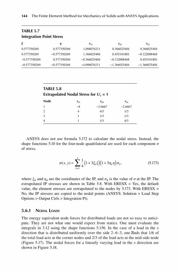
144 The Finite Element Method for Mechanics of Solids with ANSYS Applications
ANSYS does not use formula 5.172 to calculate the nodal stress. Instead, the shape functions 5.10 for the four-node quadrilateral are used for each component σ of stress,
σ ξ ξ η η σ( , )x y k k k
k
= +( ) +( )=
∑ 14
1 3 1 31
4
,
(5.173)
where ξK and ηK are the coordinates of the IP, and σK is the value of σ at the IP. The extrapolated IP stresses are shown in Table 5.8. With ERESX = Yes, the default value, the element stresses are extrapolated to the nodes by 5.173. With ERESX = No, the IP stresses are copied to the nodal points (ANSYS: Solution > Load Step Options > Output Ctrls > Integration Pt).
5.6.1 nodal loadS
The energy equivalent node forces for distributed loads are not so easy to antici-pate. They are not what one would expect from statics. One must evaluate the integrals in 3.12 using the shape functions 5.156. In the case of a load in the x direction that is distributed uniformly over the side 2–6–3, one finds that 1/6 of the total load acts at the corner nodes and 2/3 of the load acts at the mid-side node (Figure 5.17). The nodal forces for a linearly varying load in the x direction are shown in Figure 5.18.
taBle 5.8extrapolated nodal Stress for U1 = 1
node τ11 τ22 τ12
1 −8 −2.6667 −2.6667
2 4 4/3 1/3
3 1 1/3 1/3
4 1 1/3 4/3
taBle 5.7Integration point Stress
ξ η τ11 τ22 τ12
0.577350269 0.577350269 1.098076211 0.366025404 0.366025404
0.577350269 −0.577350269 1.366025404 0.455341801 −0.122008468
−0.577350269 0.577350269 −0.366025404 −0.122008468 0.455341801
−0.577350269 −0.577350269 −4.098076211 −1.366025404 −1.366025404

The Quadrilateral and the Hexahedron 145
5.6.2 plane StreSS exaMple: pure Bending
In order to test a finite element implementation, we need a nontrivial problem for which the exact solution is known. The problem diagrammed in Figure 5.19 has the following solution and can be used as a test problem.
u x ypxy
E
v x yp
Ex y
py
( , ) ,
( , ) ,
,
,
= −
= +( )= −
=
2
0
2 2
11
22
ν
τ
τ
τ112 0= .
(5.174)
Since the element displacement field (5.6.5) is complete in second-order terms, a one-element model will provide an exact solution if exact integration is used. Two-point integration also gives an exact result.
5.6.3 plane StreSS exaMple: Bending with Shear
A second example (Figure 5.20) for which the exact solution is known was analyzed in Section 5.1.3 using the four-node element. The exact solution 2.41 for plane stress or plane strain is
1 2
34
b
5
6
7
8
Actual load FE conforming
p
pb6
pb6
2pb3
η
ξ
fIgure 5.17 Node forces for a uniform load.
Actual loading FE conforming
p
p
b
pb
pb
6
6
0
fIgure 5.18 Nodal forces for linear load.

146 The Finite Element Method for Mechanics of Solids with ANSYS Applications
σ
σ
τ
x
y
xy
Pxy
c
Pc
y
c
=
=
= −
3
2
0
34
1
3
2
2
,
,
.
(5.175)
The displacements for plane stress are given in 2.42.We will now solve this problem using the eight-node element. The finite element
solution is not exact in this case because of the cubic variation in displacements as shown in 2.142. Since there is antisymmetry about the x axis, we only need to con-sider the upper half of the body and the antisymmetry conditions on the x axis as shown in Figure 5.21. Note the change in coordinates between Figures 5.20 and 5.21. For c = 1, L = 10, P = 20, the loads are as shown. The antisymmetry conditions require that the x displacement and the normal stress vector are zero along the x axis. To pre-vent rigid body displacement, we can set the y displacement to zero at the origin and set the x displacement to zero at the upper left corner. With these support conditions, the displacement at the centerline of the free end (x = L, y = 0) is given by 2.44:
v LPL
EI
c
L( , )
( ).0
31
4 52
1 02833 2
2= + +
=ν
(5.176)
for E = 10,000, ν = 1/3. Using a 50 (wide) by 10 (high) mesh of 500 eight-node ele-ments, we obtain a displacement of 1.0243, an error of 0.39%. The calculated nodal stress is shown in Figures 5.22 and 5.23. The maximum σx = 291, an error of 3%. The maximum τxy = 15.01, an error of 0.07%. The distribution closely follows the exact solution 5.175 except near the corner where the particular support condition used perturbs the numerical solution.
u(0,y) = 0
v(0,0) = 0
yx
τ11 = –py
fIgure 5.19 Plane stress bending.
σx
τxy τxy
2c x
y
L
fIgure 5.20 Plane stress bending with shear.

The Quadrilateral and the Hexahedron 147
σ = 300y
y
x
τ = 15 – 15y2 τ = 15 – 15y2
fIgure 5.21 Bending with shear: finite element model.
0
300
250
200
150
100
50
00.1 0.2 0.3 0.4 0.5
y0.6 0.7 0.8 0.9 1
σx
fIgure 5.22 Bending with shear: σx at supported end.
0
16
14
12
10
8
6
4
2
0
–2
–40.1 0.2 0.3 0.4 0.5
y0.6 0.7 0.8 0.9 1
τxy
fIgure 5.23 Bending with shear: τxy at supported end.
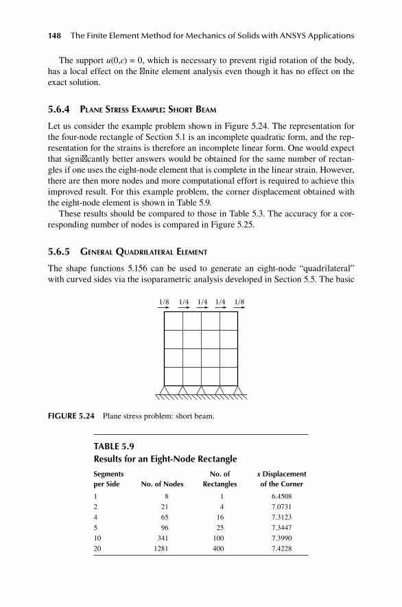
148 The Finite Element Method for Mechanics of Solids with ANSYS Applications
The support u(0,c) = 0, which is necessary to prevent rigid rotation of the body, has a local effect on the finite element analysis even though it has no effect on the exact solution.
5.6.4 plane StreSS exaMple: Short BeaM
Let us consider the example problem shown in Figure 5.24. The representation for the four-node rectangle of Section 5.1 is an incomplete quadratic form, and the rep-resentation for the strains is therefore an incomplete linear form. One would expect that significantly better answers would be obtained for the same number of rectan-gles if one uses the eight-node element that is complete in the linear strain. However, there are then more nodes and more computational effort is required to achieve this improved result. For this example problem, the corner displacement obtained with the eight-node element is shown in Table 5.9.
These results should be compared to those in Table 5.3. The accuracy for a cor-responding number of nodes is compared in Figure 5.25.
5.6.5 general quadrilateral eleMent
The shape functions 5.156 can be used to generate an eight-node “quadrilateral” with curved sides via the isoparametric analysis developed in Section 5.5. The basic
1/81/8 1/4 1/4 1/4
fIgure 5.24 Plane stress problem: short beam.
taBle 5.9results for an eight-node rectangle
Segments per Side no. of nodes
no. of rectangles
x displacement of the corner
1 8 1 6.4508
2 21 4 7.0731
4 65 16 7.3123
5 96 25 7.3447
10 341 100 7.3990
20 1281 400 7.4228

The Quadrilateral and the Hexahedron 149
equations have the same form as in Chapter 15, but with the range of summation for the node index being 8 in place of 4.
The natural coordinate system (ξ,η) defined by the inverse of relation 5.155 is truly a curved system and numerical integration is a necessity. The order of inte-gration must be high enough to provide accuracy without being too costly in com-puting time. Integration of order two in ξ and η, four IPs, is most commonly used: ξ = ±1 3/ ,η = ±1 3/ .
The sides of the general element are curved. Consider, for example, the edge 2–6–3, where ξ = 1. The mapping defined by the shape functions becomes
x X X X
y Y
= − − + −( ) + +
= − −
12
1 112
1
12
1
22
6 3
2
( ) ( ) ,
( )
η η η η η
η η ++ −( ) + +112
126 3η η ηY Y( ) .
(5.177)
Since the coordinates of points 2, 3, and 6 can be chosen independently, we see that the side 2–6–3 is in general a quadratic curve determined by the coordinates of the three nodes. This offers some advantage in fitting curved boundaries with a small number of elements, but there is a cost in increased complexity of the model.
5.7 eIght-node Block
The 3D extension of the four-node rectangle is an eight-node brick element (Figure 5.26). The side lengths and local rectangular Cartesian coordinates are
− ≤ ≤ − ≤ ≤ − ≤ ≤a
xa b
yb c
zc
2 2 2 2 2 2, , .
(5.178)
Log nodes
Disp
lace
men
t
8-Node Rect.
4-Node Rect.
0
8
7.5
7
6.5
6
5.5
5
4.5
40.5 1.5 2 2.5 3.531
fIgure 5.25 Convergence for short beam.
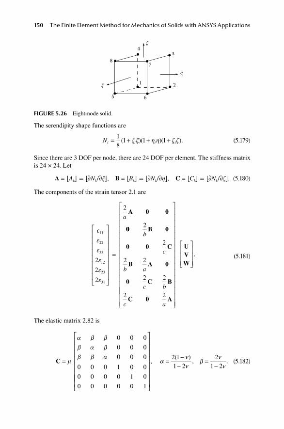
150 The Finite Element Method for Mechanics of Solids with ANSYS Applications
The serendipity shape functions are
Ni i i i= + + +1
81 1 1( )( )( )ξ ξ η η ζ ζ .
(5.179)
Since there are 3 DOF per node, there are 24 DOF per element. The stiffness matrix is 24 × 24. Let
A = ⌊Ak⌋ = ⌊∂Nk/∂ξ⌋, B = ⌊Bk⌋ = ⌊∂Nk/∂η⌋, C = ⌊Ck⌋ = ⌊∂Nk/∂ζ⌋. (5.180)
The components of the strain tensor 2.1 are
ε
ε
ε
ε
ε
ε
11
22
33
12
23
31
2
2
2
2
=
aA 0 0
00 B 0
0 0 C
B A 0
0 C B
C 0 A
2
2
2 2
2 2
2 2
b
c
b a
c b
c a
UVW
.
(5.181)
The elastic matrix 2.82 is
C =
µ
α β ββ α ββ β α
0 0 0
0 0 0
0 0 0
0 0 0 1 0 0
0 0 0 0 1 0
0 0 0 0 0 1
= −−
=−
,( )
, .ανν
βν
ν2 11 2
21 2
(5.182)
3
2
7
4
8
5 6
1ξ
ζ
ɳ
fIgure 5.26 Eight-node solid.

The Quadrilateral and the Hexahedron 151
The stiffness matrix 3.24 is therefore
U V W
k
A A A
A=
+ +
µ β
α
αabca b c
ab2
1 12 11 2 22 2 33
21
symmetric
bb c a
ab ab c a
2 22 2 33 2 11
31 32 2 33 2 1
1 1
1
A A A
A A A A
+ +
+
β β α
11 2 221+
,
bA
(5.183)
where
A A A
A
11
22
172
3 3= = + + ∫∫∫ T d d dξ η ζ ξ ξ η η ζ ζk m k m k m( )( )
== = + +
=
∫∫∫ B
A C
T d d dB ξ η ζ η η ζ ζ ξ ξ172
3 3
33
k m k m k m( )( )
TT d d dC
A A
ξ η ζ ζ ζ ξ ξ η η= + +
=
∫∫∫ 172
3 3
12 21
k m k m k m( )( )
TTk m k m
T
= = +
= =
∫∫∫ A B
A A B C
T
T
d d dξ η ζ ξ η ζ ζ124
3
23 32
( )
dd d d
d d dT
ξ η ζ η ζ ξ ξ
ξ η
∫∫∫ = +
= =
124
3
31 13
k m k m
T
( )
A A C A ζζ ζ ξ η η∫∫∫ = + 124
3k m k m( ) .
(5.184)
For the case a = b = c = 2, ν = 1/3, α = 4, β = 2, the first column of the element stiff-ness matrix is
[ ]FXk =
−−
−−
µ24
32161288
1280
=
−−
−−
, [ ]FYk
µ24
124
1246262
=−
−−−
, [ ]FZk
µ24
124264
1262
.
(5.185)

152 The Finite Element Method for Mechanics of Solids with ANSYS Applications
This agrees with ANSYS element SOLID45 without extra DOFs. Although this ele-ment is very instructive and valuable for historical reasons, ANSYS is phasing it out. I will continue to refer to it as a synonym for an analysis based on the developments of this section.
5.8 tWenty-node SolId
The eight-node quadrilateral becomes a 20-node solid (Figure 5.27). The shape functions are as follows.
Nodes 1 8:− = + + + + +Ni i i i i i
18
1 1 1( )( )( )(ξ ξ η η ζ ζ ξ ξ η η ζ ii
i iN
ζ
ξ ξ η
−
= + −
2
14
1 1 2
).
( )( )(Nodes 9,11,13,15: 11
14
1 1
+
= + +
ζ ζ
ξ ξ η
i
i i iN
).
( )(Nodes 10,12,14,16: ηη ζ
ξ η
)( ).
( )(
1
14
1 1
2
2
−
= − +Nodes 17,18,19, 20: Ni ii iη ζ ζ)( ).1 +
(5.186)
This is the basis for the ANSYS element 186.Many other elements have been developed for both two and three dimensions.9
Those included here are the most commonly used.
5.9 SIngularIty eleMent
We have seen that singularities in the solution to boundary value problems may occur when there are discontinuities in the boundary conditions. The solution for stress near the singularity is not very good if we use standard elements. The solution can be improved by using elements with the theoretical singularity built into them. As an example, let us consider a six-node rectangle for which two of the side nodes
10
3
2
η
11ζ
197
14
18
9
6135
16
820
4
1512
117ξ
fIgure 5.27 Twenty-node solid.

The Quadrilateral and the Hexahedron 153
are placed at the quarter point of a side rather than at the midpoint. This will result in a singularity in strain at the selected special corner.
We first generate a six-node triangle by collapsing the eight-node rectangle shown in Figure 5.16 into a six-node triangle (Figure 5.28). The mapping from the (ξ,η) plane onto the (x,y) plane for the rectangle is
x N X y N Yi i i i= =∑ ∑1
8
1
8
, ,
(5.187)
where the shape functions are defined by 5.156. Note that the mapping can be used even if the side nodes are not at the mid-point of the side. Now, collapse nodes 4 and 8 onto node 1: X4 = X8 = X1 and Y4 = Y8 = Y1 and renumber the remaining nodes as in Figure 5.28. We have
x X X= − −( ) + +( ) −( ) − −( ) + +( ) +(12
114
1 1 114
1 11 2ξ ξ ξ η ξ η ξ η )) + −( )
+ −( ) −( ) + +( ) −( ) +
ξ η
ξ η ξ η
1
12
1 112
1 112
1
3
24
24
X
X X −−( ) +( )ξ η261 X .
(5.188)
The formula for y is similar. This induces shape functions for the triangle:
N N
N
1 2
3
12
114
1 1 1
14
1 1
= − −( ) = +( ) −( ) − −( )
= +( )
ξ ξ ξ η ξ η
ξ
, ,
++( ) + −( ) = −( ) −( )
= +( ) −( )
η ξ η ξ η
ξ η
112
1 1
12
1 1
42
52
, ,
,
N
N NN621
21 1= −( ) +( )ξ η .
(5.189)
l
l
x
23hh44
4
5
3
16
y
fIgure 5.28 Singularity triangle.

154 The Finite Element Method for Mechanics of Solids with ANSYS Applications
For the symmetric geometry shown in Figure 5.28, we find
x h y
l= + = +( )( ) , .1 44
12 2ξ η ξ/
(5.190)
The lines for which η is constant are radial lines through node 1. The lines for which ξ is constant are the lines x is constant. The displacements are
u N U N U N U N U N U N U
v N V N V N V
= + + + + +
= + +
1 1 2 2 3 3 4 4 5 5 6 6
1 1 2 2 3
,
33 4 4 5 5 6 6+ + +N V N V N V . (5.191)
Calculation of the displacement gradients shows a 1 / r singularity, where r is the radial distance from node 1. For example, consider the line y = 0, η = 0, and x = r; we then find
u U U U U U U= − −( ) + + − −( ) + + + −1
41 2 2 2
12
112
121 2 3 4 6 5ξ ξ ξ( ) ( )) .U1
(5.192)
Using 5.190, we find the 1/ r singularity in the displacement gradient:
∂∂
= +u
xc
c
r1
2 .
(5.193)
Similar results are found for the other derivatives. This element is useful for the analysis of structures with crack surfaces.
5.10 MIxed u–p eleMentS
For nearly incompressible materials, we can introduce the mean stress as a separate unknown. The appropriate virtual work formulas are 3.113 for three dimensions and 3.21 or 3.24 for plane strain. Shape functions are required for the displacements and for the mean pressure, and they need not be the same functions.
5.10.1 plane Strain
For plane strain, the virtual work formula is 3.126:
2µ εκαβ
α
β
α
αααe
ux
pux
pp A
∂∂
− ∂∂
− +
∫ dA
== +∫ ∫T u s b u Aα α α αd dC A
. (5.194)
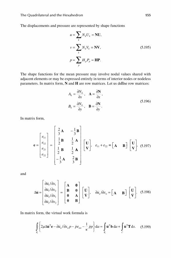
The Quadrilateral and the Hexahedron 155
The displacements and pressure are represented by shape functions
u N U
v N V
p H P
k k
k
k k
k
p p
p
= =
= =
= =
∑∑∑
NU
NV
HP
,
,
.
(5.195)
The shape functions for the mean pressure may involve nodal values shared with adjacent elements or may be expressed entirely in terms of interior nodes or nodeless parameters. In matrix form, N and H are row matrices. Let us define row matrices:
AN
x x
BN
y y
kk
kk
= ∂∂
= ∂∂
= ∂∂
= ∂∂
, ,
, .
AN
BN
(5.196)
In matrix form,
e
A B
B A
B=
=
−e
e
e
e
11
12
21
22
23
13
12
12
12
12
AA
A B
UV
−
+
13
23
11 22, ε ε ==
A B
UV
,
(5.197)
and
∆u
A
=
∂ ∂∂ ∂∂ ∂∂ ∂
=
u x
u x
u x
u x
1 1
1 2
2 1
2 2
/
/
/
/
00B 00 A0 B
UV
A BUV
∂ ∂ =
, u xα α/
. (5.198)
In matrix form, the virtual work formula is
21
µ εκα α αα∆u e u b uT T/ d d− ∂ ∂ − −
= +∫ ∫u x p p pp a aT
R R
TT dsC∫ .
(5.199)

156 The Finite Element Method for Mechanics of Solids with ANSYS Applications
Substitution of (5.195)–(5.198) gives
U V K UV
K P P K UV
T T T
+
+
uu up pu +
≡K P U V Fpp [ ] ,T T
(5.200)
where
KA A B B B A A B
A B B A B Buu =
+ −
− +2
23
12
12
13
12
13
23
12
µ
T T T T
T T T AA AT
d
∫ aR
,
(5.201)
K K AB
Hpu up aTT
Td= = −
∫
R
.
(5.202)
K H Hpp a= − ∫ 1κ
T dR
.
(5.203)
Equating the coefficients of the virtual displacements, we find the fundamental rela-tions for the element:
K K
K KDP
F0
uu up
pu pp
=
.
(5.204)
There are now two possible models. If the interpolation for p uses nodes that are shared with adjacent elements, the element stiffness matrix defined by 5.204 must be merged into the global stiffness matrix. The pressure parameters P are then determined along with the displacement parameters by solving the global equations.
However, if the interpolation for p uses nodeless parameters or internal nodal parameters, then the pressure parameters P can be eliminated at the element level by static condensation. Partitioning 5.204 gives
K D K P F
K D K P 0
uu up
pu pp
+ =
+ =
,
. (5.205)

The Quadrilateral and the Hexahedron 157
Eliminating P gives
KD = F, (5.206)
where
K K K K K= − −
uu up pp pu1 .
(5.207)
The analysis then proceeds as in the pure displacement model but using the stiffness matrix defined by 5.207.
In practice, if the material is nearly incompressible the model is typically too stiff and may “lock” unless the interpolation or the integration of the pressure terms is of lower order than for the displacement terms. The simplest usable case is the following four-node element. The displacements are interpolated using the serendipity functions 5.10 that are linear in (x,y). The pressure is interpolated by one order lower, that is, by a constant pressure in each element. In this case, we have the following results.
A B H= +
= +
=1
21
12
1 1a bk k k kξ η η η ξ ξ( ) , ( ) , [ ]..
(5.208)
For the rectangular element, the integration can be easily done. We find the stiffness matrix K defined by 5.207 to be as follows.
KK K
K K=
11 12
21 22
,
(5.209)
where each submatrix is 4 × 4 with elements:
K11 364 3 3 3
4= + + +
+µξ ξ η η η η ξ ξ
κb
a
a
bk m k m k m k m( ) ( )bb
a k mξ ξ
,
(5.210)
K22 364 3 3 3
4= + + +
+µη η ξ ξ ξ ξ η η
κa
b
b
ak m k m k m k m( ) ( )aa
b k mη η
,
(5.211)
K K12 21 12
3 24
T = = − +
µξ η η ξ
κη ξ( ) .k m k m k m
(5.212)
In the case where a = b, ν = 1/3, κ = 8μ/3,
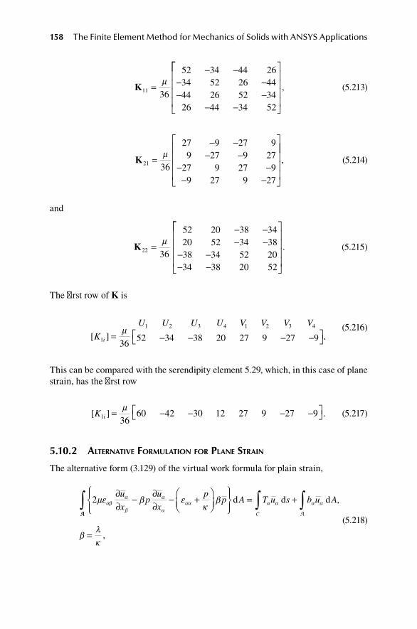
158 The Finite Element Method for Mechanics of Solids with ANSYS Applications
K11 36
52 34 44 2634 52 26 4444 26 52 3426 44 34 52
=
− −− −− −
− −
µ
,
(5.213)
K21 36
27 9 27 99 27 9 27
27 9 27 99 27 9 27
=
− −− −
− −− −
µ
,
(5.214)
and
K22 36
52 20 38 3420 52 34 3838 34 52 2034 38 20 52
=
− −− −
− −− −
µ
. (5.215)
The first row of K is
U U U U V V V V
K i
1 2 3 4 1 2 3 4
1 3652 34 38 20 27 9 27 9[ ] = − − − −
µ.. (5.216)
This can be compared with the serendipity element 5.29, which, in this case of plane strain, has the first row
[ ] .K i1 36
60 42 30 12 27 9 27 9= − − − − µ
(5.217)
5.10.2 alternatiVe forMulation for plane Strain
The alternative form (3.129) of the virtual work formula for plain strain,
2µε β εκ
βαβα
β
α
ααα
∂∂
− ∂∂
− +
u
xp
u
x
pp Ad
AA C A∫ ∫ ∫= +
=
T u s b u Aα α α α
βλκ
d d ,
,
(5.218)
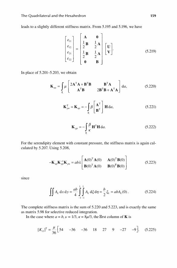
The Quadrilateral and the Hexahedron 159
leads to a slightly different stiffness matrix. From 5.195 and 5.196, we have
ε
ε
ε
ε
11
12
21
22
12
12
12
12
=
A 0
B A
B A
0 B
UV
.
(5.219)
In place of 5.201–5.203, we obtain
K A A B B B AA B B B A A
uu a= ++
∫ µ 2
2
T T T
T T Td
R
,
(5.220)
K K AB
Hpu up aTT
Td= = −
∫ β
R
,
(5.221)
K H Hpp a= − ∫ βκ
T dR
.
(5.222)
For the serendipity element with constant pressure, the stiffness matrix is again cal-culated by 5.207. Using 5.208,
− =−K K KA A A B
B A Bup pp pu ab1 0 0 0 0
0 0 0λ
( ) ( ) ( ) ( )
( ) ( ) ( )
T T
T TT B( )0
(5.223)
since
A x yab
Ab
abAk k k kd d d d∫∫ ∫∫= = =−−
4 20
1
1
1
1
ξ η ξ ( ) . (5.224)
The complete stiffness matrix is the sum of 5.220 and 5.223, and is exactly the same as matrix 5.98 for selective reduced integration.
In the case where a = b, ν = 1/3, κ = 8μ/3, the first column of K is
[ ] .Ki1 36
54 36 36 18 27 9 27 9T = − − − − µ
(5.225)

160 The Finite Element Method for Mechanics of Solids with ANSYS Applications
This agrees with ANSYS element Plane182 mixed U/P method with the Enhanced Strain option.
5.10.3 3d eleMentS
The modified virtual work formula 3.110 is
2µ δ ε εκ
e pp
p V T uij ij ij i i−( ) − +
=∫ d d
V
AA b u Vi i+∫ ∫A V
d ,
(5.226)
The displacements are represented by shape functions
u N U v N V
w N W p H P
k k
k
k k
k
k k
k
p p
p
= = = =
= = = =
∑ ∑∑ ∑
NU NV
NW HP
, ,
, ..
(5.227)
We define row matrices:
AN
x x
BN
y y
CN
y y
kk
kk
kk
= ∂∂
= ∂∂
= ∂∂
= ∂∂
= ∂∂
= ∂∂
, ,
, ,
,
AN
BN
CN..
(5.228)
The deviatoric strains and volumetric strain are then
e
e
e
e
e
e
11
22
33
12
23
31
23
13
=
− −A B 113
13
23
13
13
13
23
12
1212
12
12
12
C
A B C
A B C
B A 0
0 C B
C 0 A
− −
− −
UVW
, εεii =
A B CUVW
.
(5.229)
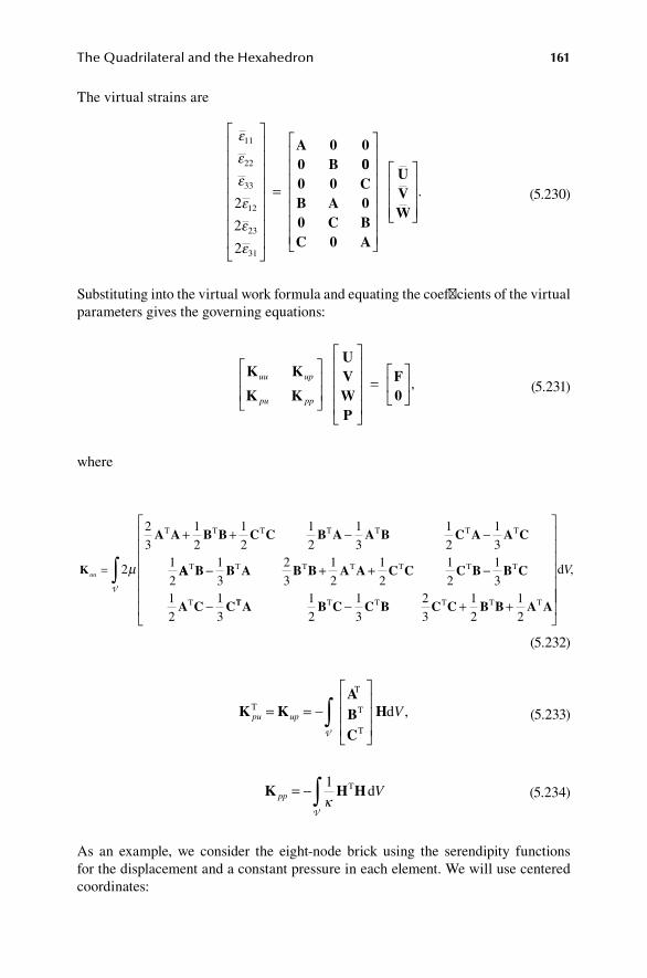
The Quadrilateral and the Hexahedron 161
The virtual strains are
ε
ε
ε
ε
ε
ε
11
22
33
12
23
31
2
2
2
=
A 0 00 B 000 0 CB A 00 C BC 0 A
UVW
.
(5.230)
Substituting into the virtual work formula and equating the coefficients of the virtual parameters gives the governing equations:
K K
K K
UVWP
F0
uu up
pu pp
=
,
(5.231)
where
K
A A B B C C B A A B C A A C
uu =
+ + − −
2
2
3
1
2
1
2
1
2
1
3
1
2
1
31
2µ
T T T T T T T
AA B B A B B A A C C C B B C
A C C
T T T T T T T
T
− + + −
−
1
3
2
3
1
2
1
2
1
2
1
31
2
1
3TT T T T T TA B C C B C C B B A A
1
2
1
3
2
3
1
2
1
2− + +
∫ dV,V
(5.232)
K KABC
Hpu up VT
T
T
T
d= = −
∫V
,
(5.233)
K H Hpp V= − ∫ 1κ
T dV
(5.234)
As an example, we consider the eight-node brick using the serendipity functions for the displacement and a constant pressure in each element. We will use centered coordinates:

162 The Finite Element Method for Mechanics of Solids with ANSYS Applications
− ≤ ≤ − ≤ ≤ − ≤ ≤a
xa b
yb c
zc
2 2 2 2 2 2, , .
(5.235)
The serendipity shape functions for the displacements are
Ni i i i= + + +1
81 1 1( )( )( )ξ ξ η η ζ ζ .
(5.236)
Therefore,
A
B
= ∂ ∂ = + +
= ∂ ∂
2 21 1
2
aN
a
bN
k k k k
k
/
/
ξ ξ η η ζ ζ( )( ) ,
ηη η ζ ζ ξ ξ
ζ
= + +
= ∂ ∂ =
21 1
2 2
b
cN
c
k k k
k
( )( ) ,
C / ζζ ξ ξ η ηk k k( )( ) .1 1+ +
(5.237)
Therefore,
A A
A B
T
T
d
d
Vabc
a
V
k m k m k m
V
V
∫ = + + 1443 3
2ξ ξ η η ζ ζ( )( ) ,
∫∫ = + abc
ab k m k m483ξ η ζ ζ( ) .
(5.238)
The other factors can be written down by cyclic permutation of (ξ,η,ζ) and (a,b,c). For constant pressure in each element, H = [1].
For the case a = b = c = 2, ν = 1/3, κ = 8μ/3, the first column of the element stiff-ness matrix is
[ ]
.
.
FXk =−−−−
µ27
29105
101114 51414 5
=
−−
−−
, [ ]
.
.
.
.
.
.
FYk
µ27
10 51 55 259 751 5
10 59..
.
, [ ]
.
755 25
27
10 59
=FZk
µ
..
.
.
.
.
.
.
755 251 51 55 259 75
10 5
−−
−−
.
(5.239)
This can be compared with ANSYS element SOLID185, U–P method, Full Integration.

The Quadrilateral and the Hexahedron 163
5.11 proBleMS
1. Given: The stiffness matrix for a plane stress square element of Figure 5.29 is given by
k =
− − − −
− − − −
− −
6 1 5 3 1 5 3 1 5 0 1 5
6 1 5 0 1 5 3 1 5 3
6 1 5 0 1
. . . .
. . .
. .. .
. .
. .
.
.
5 3 1 5
6 1 5 3 1 5 3
6 1 5 3 1 5
6 1 5 0
6 1 5
6
−
− −
− −
−
U
V
U
V
U
V
U
V
1
1
2
2
3
3
4
4
.
(5.240)
A plane stress problem is modeled by two elements as shown in Figure 5.30. Determine the global stiffness matrix K for the unrestrained body. Answer: Stiffness matrix for element 1 with nodes 1–2–5–6:
D D D D D D D D1 2 3 4 9 10 11 12
1
6 1 5 3 1 5 3 1 5 0 1 5
6 1 5 0
k =
− − − −. . . .
. −− − − −
− − −
− −
− −
1 5 3 1 5 3
6 1 5 0 1 5 3 1 5
6 1 5 3 1 5 3
6 1 5 3 1
. .
. . .
. .
. ..
.
.
5
6 1 5 0
6 1 5
6
−
F11
2
3
4
9
10
11
12
F
F
F
F
F
F
F
.
x
2
y
1
34
1
1
fIgure 5.29 Four-node element.

164 The Finite Element Method for Mechanics of Solids with ANSYS Applications
Stiffness matrix for element 2 with nodes 2–3–4–5:
D D D D D D D D3 4 5 6 7 8 9 10
2
6 1 5 3 1 5 3 1 5 0 1 5
6 1 5 0 1
k =
− − − −
−
. . . .
. .. .
. . .
. .
. .
5 3 1 5 3
6 1 5 0 1 5 3 1 5
6 1 5 3 1 5 3
6 1 5 3 1 5
− − −
− − −
− −
− −
66 1 5 0
6 1 5
6
3
.
.−
F
F44
5
6
7
8
9
10
F
F
F
F
F
F
.
Global stiffness matrix after merging element 1:
D D D D D D D D D D D D1 2 3 4 5 6 7 8 9 10 11 12
6 1 5 3
.
K =
− −11 5 3 1 5 0 1 5
6 1 5 0 1 5 3 1 5 3
6 1 5 0 1 5 3 1 5
6
. . .
. . .
. . .
− −
− − − −
− − −
11 5 3 1 5 3
6 1 5 3 1 5
6 1 5 0
6 1 5
6
. .
. .
.
.
− −
− −
−
F
F
F
F
F
F
F
1
2
3
4
5
6
77
8
9
10
11
12
F
F
F
F
F
.
6
x
y
32
1
1
1
4 5
1
fIgure 5.30 Two-element model (a).
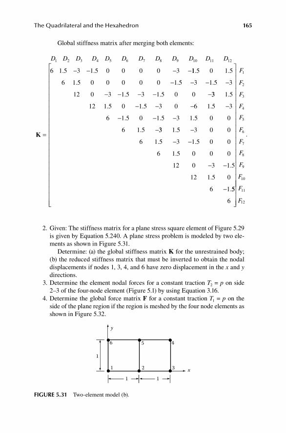
The Quadrilateral and the Hexahedron 165
Global stiffness matrix after merging both elements:
D D D D D D D D D D D D1 2 3 4 5 6 7 8 9 10 11 12
6 1 5 3 1 5 0 0 0 0 3
. .
K =
− − − −11 5 0 1 5
6 1 5 0 0 0 0 0 1 5 3 1 5 3
12 0 3 1 5 3 1 5 0 0
. .
. . .
. .
− − − −
− − − − −33 1 5
12 1 5 0 1 5 3 0 6 1 5 3
6 1 5 0 1 5 3 1 5 0 0
6 1 5
.
. . .
. . .
.
− − − −
− − −
−33 1 5 3 0 0
6 1 5 3 1 5 0 0
6 1 5 0 0 0
12 0 3 1 5
12 1 5 0
6 1
.
. .
.
.
.
.
−
− −
− −
− 55
6
F
F
F
F
F
F
F
F
F
F
F
F
1
2
3
4
5
6
7
8
9
10
11
12
.
2. Given: The stiffness matrix for a plane stress square element of Figure 5.29 is given by Equation 5.240. A plane stress problem is modeled by two ele-ments as shown in Figure 5.31.
Determine: (a) the global stiffness matrix K for the unrestrained body; (b) the reduced stiffness matrix that must be inverted to obtain the nodal displacements if nodes 1, 3, 4, and 6 have zero displacement in the x and y directions.
3. Determine the element nodal forces for a constant traction T2 = p on side 2–3 of the four-node element (Figure 5.1) by using Equation 3.16.
4. Determine the global force matrix F for a constant traction T1 = p on the side of the plane region if the region is meshed by the four node elements as shown in Figure 5.32.
4
x
y
32
1
1
1
6 5
1
fIgure 5.31 Two-element model (b).

166 The Finite Element Method for Mechanics of Solids with ANSYS Applications
5. Solve the plane stress problem diagrammed in Figure 5.33 for the corner displacement using one 4-node square element numbered as shown in Figure 5.29 without using ANSYS.
Answers:
K =
−−
− −− − −
µ24
3212 3220 0 320 4 12 32
16 12 4 0 3212 16 0 20 12 3224 0 16 12 20 0 320 20 12 16 0 4 12 32
− −− − −
,
U
pa
EV
pa
E= =
14
32, .
6. Use ANSYS to solve the plane stress problem shown in Figure 5.33 for a = 1, p = 1, E = 100, ν = 0.3, using 16 equal-size four-node rectangles. Input the nodal forces by hand. Submit a list of nodal displacements. (See Section 15.7.)
a
p
a
22
31
1 xy
8
63
7 44
9 5
fIgure 5.32 Four-element model.
x
p
by
a
fIgure 5.33 Short beam problem.

The Quadrilateral and the Hexahedron 167
7. Derive the generalized nodal forces for a uniform body force b1 = 1 over a four-node rectangular element in plane stress.
8. Consider the plane stress problem shown in Figure 5.34. Given: a = 10, b = 2, p = 1, E = 1, ν = 0.3. The origin has zero displace-
ment and ν = 0 at point (a,0). (a) Solve this problem using ANSYS with element Plane182 and square elements of dimension 1/2. (b) Compare the displacement UY and the stress SX along line x = 5 with the exact solution discussed in Section 2.1.11. (See Section 15.9.)
9. Solve problem 8 using the eight-node element Plane183. Submit the nodal displacements and nodal stress along line x = 5, and compare the result with the exact solution.
10. Given the shape functions for the four-node rectangle (5.10), obtain the shape functions for a right triangle by setting X1 = X4, Y1 = Y4, U1 = U4, and V1 = V4. Show that these shape functions agree with those for the three-node triangle if ξ = 2ζ2 + 2ζ3 – 1 and η = (ζ3 – ζ2)/(ζ3 + ζ2).
11. Determine the nodal forces for T1 = constant, on the side ξ = 1 of the eight-node rectangle (Figure 5.16).
12. Solve the plane strain bending problem (Section 5.1.3) using the Plane183 element and a 4 × 8 mesh for c = 2, L = 16, i = 8192, ν = 0.3. Compare the displacement with that for Plane182 elements (Table 5.2) and with the exact result. (See Section 15.10.)
13. Solve the plane strain bending problem (Section 5.1.3) using the Plane182 element with the U–P formulation (OPTIONS > K8 = MIXED U/P) and a
pp
b
pp
a
xy
fIgure 5.34 Plane stress problem.
S
2a
y
rx2b
fIgure 5.35 Sheet with a hole.

168 The Finite Element Method for Mechanics of Solids with ANSYS Applications
4 × 8 mesh for c = 2, L = 16, E = 8192, ν = 0.499. Compare the y displace-ment with that for Plane42 elements (Table 5.2) and with the exact result.
14. Solve problem 6 by ANSYS using SURF153 to apply the distributed load. (See Section 15.11.)
15. Show that the displacement along an edge of the eight-node rectangle varies quadratically and is therefore uniquely determined by the values at the three nodes on the edge. (This ensures continuity between elements by matching nodal displacements.)
16. Determine shape functions for a triangle with mid-side nodes from the eight-node quadrilateral by collapsing nodes 1, 4, and 8 together.
17. A sheet with a central hole (see Figure 5.35) is stretched by a uniform edge stress S resulting in a stress concentration at the hole. In nondimensional variables: S = 100, a = 20, b = 10, r = 5, E = 1, ν = 0.3. Use ANSYS with element Plane182 to investigate the stress concentration (see Section 15.12). Use 1/4 of the sheet and symmetry conditions (Figure 5.36).
18. Solve problem 17 using element Plane183. Plot stress SX along x = 0.
19. Evaluate A AA
2 1T da∫ for the four-node rectangle (Section 5.1).
20. For the reduced integration on the λ term, evaluate fully the λ part of the element stiffness matrix: k2 = abA(0,0)TC2A(0,0).
21. Calculate all components of the consistent element force matrix for a uni-formly distributed load p in the x direction on side ξ = 1 of the eight-node rectangle.
22. Determine matrix B for the Wilson–Taylor four-node rectangle (see Section 5.2.1).
referenceS
1. Wilson, E. L. et al., Incompatible displacement models, Numerical and Computer Methods in Structural Mechanics, ed. S. J. Fenves et al., 43–57, Academic Press, New York, 1973.
2. Taylor, R. L., P. J. Beresford, and E. L. Wilson, A non-conforming element for stress analysis, Int. J. Numer. Meth. Eng., 10, 1211–1219, 1976.
UY = 0
R = 2
x
y
UX
= 0
SX =
100
10
10
fIgure 5.36 Plane stress: sheet with a hole
The Quadrilateral and the Hexahedron 169
3. Simo, J. C., and M. S. Rifai, A class of mixed assumed strain methods and the method of incompatible modes, Int. J. Numer. Meth. Eng., 29, 1595–1638, 1990.
4. Hughes, T. J. R., Generalization of selective integration procedures to anisotropic and nonlinear media, Int. J. Numer. Meth. Eng., 15, 1413–1418, 1980.
5. Kosloff, D., and G. A. Frazier, Treatment of hourglass patterns in low order finite ele-ment codes, Int. J. Numer. Anal. Meth. Geomech., 2, 57–72, 1978.
6. Flanagan, D. P., and T. Belytschko, A uniform strain hexahedron and quadrilateral with orthogonal hourglass control, Int. J. Numer. Meth. Eng., 17, 679–706, 1981.
7. Kardestuncer, H., and D. H. Norrie, eds., Finite Element Handbook, 2.103, McGraw-Hill, New York, 1987.
8. Irons, B. M., Engineering applications of numerical integration in stiffness methods, AIAA J., 4, 2035–2037, 1966.
9. Kardestuncer, H., and D. H. Norrie, eds., Finite Element Handbook, 2.121–2.131, McGraw-Hill, New York, 1987.
BIBlIography
Bathe, K. J., Finite Element Procedures, Prentice-Hall, Englewood Cliffs, NJ, 1996.Hughes, T. J. R., The Finite Element Method: Linear Static and Dynamic Finite Element
Analysis, Dover Publications, Mineola, NY, 2000.Zienkiewicz, O. C., R. L. Taylor, and J. Z. Zhu, The Finite Element Method: Its Basis and
Fundamentals, Elsevier Butterworth-Heinemann, Burlington, MA, 6th ed., 2005.Zienkiewicz, O. C., and R. L. Taylor, The Finite Element Method for Solid and Structural
Mechanics, Elsevier Butterworth-Heinemann, Burlington, MA, 6th ed., 2005.

171
6 Errors and Convergence of Finite Element Solution
6.1 general reMarkS
From the engineer’s viewpoint, the objective in the finite element method is to estab-lish an approximate solution to the boundary value problem that is sufficiently accu-rate for engineering design. That is, one hopes that the error can be made reasonably small by an analysis using the number of elements that can be handled by the avail-able computer. From the mathematician’s viewpoint, the objective is to establish a numerical procedure that ensures that any prescribed measure of error can be made as small as desired by taking enough elements, even if such calculations cannot actually be performed, that is, the mathematician seeks proof of convergence. The engineer seeks to achieve small error within the available capacity of the computer.
Error in the calculation has several sources. First of these is the simple inaccuracy of all real numerical calculations. Each machine is capable of only a finite number of digits in the representation of real numbers. Every multiplication or division there-fore introduces a round-off error. Such errors can be large if the stiffness matrix is poorly conditioned. This can happen, for example, when one portion of the body is very stiff compared with the remainder. In this case, too many nodes are being used to describe what is essentially a rigid motion.
Another source of error is approximation of boundary conditions. The conditions on the trial functions for minimizing the potential may be violated because the finite ele-ment approximation fails to exactly satisfy the boundary condition on displacement at every point. The element boundaries may not exactly match the actual boundary. Even when the shapes match, the displacements are specified only at the node points and the element may be such that the displacement boundary conditions are not exactly satisfied at all points between the nodes. This kind of error does not generally prohibit conver-gence, provided that the boundaries do match in the limit of vanishing element size.
Numerical integration will also introduce an error. It is usually a compensat-ing error because numerical integration effectively makes the model more flexible. Using a number of integration points that are less than that required for an exact inte-gration over the region can yield a better answer than is obtained by exact integration of the energy over the element. Convergence still occurs if this error vanishes with decreasing element size.
The error in calculation of the displacement or stress is, of course, greatest where those quantities vary most rapidly. For the best results with the same number of elements, one should not use a uniform element size. Smaller elements should be used where the stress is varying rapidly. As shown in the short beam example in Section 5.1.4, smaller elements should be used near the corners. The ideal element distribution is one in which

172 The Finite Element Method for Mechanics of Solids with ANSYS Applications
the error in the strain energy of an element is the same for all elements. This can be achieved by making a sequence of calculations, beginning with a uniform coarse mesh of elements, and placing more elements in regions where high displacement gradients are found. In this way, the mesh is adapted to suit the problem. There are, in fact, several computer programs that offer adaptive mesh generation.
Proof of convergence is a complicated mathematical problem in the theory of numerical analysis.1 Roughly, convergence will occur if the finite element model generates a continuous displacement field (continuity requirement), and the linear terms in a power series representation of displacement within an element are present (completeness requirement). Convergence to the true solution may occur in other cases but this must be separately established.
Theoretical studies of converge only establish that the error in displacements van-ishes with the element size. The actual magnitude of the error for any finite number of elements cannot be established. As a practical matter, the magnitude of the error is estimated by doing a series of calculations with increasingly larger numbers of ele-ments and plotting the results to see if there is an apparent limit. However, care must be taken in the interpretation of the stress calculation. Singularities can occur so that the calculated stress does not approach a limit, but just becomes larger and larger for each element subdivision without a limiting value. We have seen that such a singular-ity exists in the corner for the short beam as discussed in Section 2.1.14.
Such calculations for the displacement of the short beam example using the trian-gular element and the four-node rectangle are plotted in Figure 4.9 and Figure 5.25. The displacement does appear to be monotonically converging to a definite limit that we take to be the true solution. There is no guarantee, however, that the limit will be evident with any finite number of elements. We are forced to rely on experience and comparison to the exact solution in a few cases where the exact solution is known. In practice, one must be satisfied when the incremental improvement in displacement is a small fraction of the last calculated value. It is also possible to extrapolate the solution as described in Section 4.4.1.
Since the true solution makes the potential energy a minimum, the finite element approximation gives a larger potential energy and, in the sense that has been described in Section 3.1.5, the calculated displacements are always too small. If the elements are chosen appropriately, the numerical solution coincides with the true solution in the limit of vanishing element size. In the process of choosing increasing numbers of elements, if each successive subdivision includes the previous one as a special case, the poten-tial energy will become monotonically smaller, and the calculated displacements will become monotonically larger, that is, the finite element solution will exhibit monotonic convergence from below. This is the situation for the analysis illustrated in Figure 5.25.
In the derivation of the potential energy, it has been assumed that displacement components are continuous functions of space variables and the strains derived from displacement are continuous, except possibly for a finite number of simple jump dis-continuities. If the finite element model has this property, the elements are said to be conforming or compatible. Nonconforming elements violate the continuity require-ment at element boundaries. Cases are known where convergence occurs even for a nonconforming element, but in other cases the solution does not converge, or con-verges to a function that is not the true solution.

Errors and Convergence of Finite Element Solution 173
Nevertheless, nonconforming elements are sometimes used. In some cases, the nonconforming elements are used to obtain a more reasonable approximation to the actual state of stress. In other cases, such as for plates and shells, they may be an attempt to simplify the formulation when it is difficult to use shape functions for conforming elements, or none have been found, or the conforming elements lead to numerical difficulties.
Nonconforming elements often yield better answers for a small number of ele-ments than the more theoretically sound conforming elements. The conforming ele-ment provides a model of the structure that is always too stiff. The nonconforming element provides a means of relaxing the excessive constraints of the conforming element and therefore may achieve a better approximation—that is, the nonconform-ing element introduces a compensating error. Monotonic convergence may be lost as a result of relaxing the constraints, and the approximation provided by the noncon-forming element may sometimes give displacements that are too large.
Caution is necessary in using nonconforming elements. In the literature, some elements have been proposed that do not provide convergence, or for which conver-gence is to the wrong answer, or for which convergence depends on the shape of the elements. Nonconforming elements have a place in finite element analysis, but one must proceed carefully. Nonconforming elements are most useful for plates and shells, where continuity of first derivatives of displacement must be maintained for a conforming element, and that requirement leads to complicated formulations.
6.2 eleMent Shape lIMItS
Cubic elements in 3D and square elements or equilateral triangles in 2D generally result in equations that are well conditioned. If the element shape is greatly distorted from these ideal shapes, numerical difficulties can occur. Consequently, ANSYS has built-in checks on element shapes in the array of finite elements.2 Such highly distorted elements may occur when the free mapping algorithm is used for meshing. They can be avoided by using mapped meshing
A warning will be generated if the element shape appears distorted. After a warning, you have the option to proceed with the analysis or to alter the element grid. An error message is generated and the calculation aborted if the element is so distorted that excessive numerical errors are likely. For 2D elements, ANSYS checks the aspect ratio, deviation from parallel sides for quadrilaterals, maximum corner angle, and the ratio of the Jacobian within quadrilaterals. Automatically gen-erated meshes often result in warnings, and one has to decide whether to continue the analysis.
6.2.1 aSpect ratio
For a triangle, Figure 6.1, the aspect ratio R for node n is defined by
R
h
ann
n
=2
3,
(6.1)

174 The Finite Element Method for Mechanics of Solids with ANSYS Applications
which has a value of 1 for an equilateral triangle. The aspect ratio for the element is the largest of the three possible ratios.
For the quadrilateral element (Figure 6.2), the aspect ratio is the ratio of the sides of a rectangle prescribed by the midpoints (A, B, C, D) of the sides:
r
X X
Y YR r rB A
D C
= −−
= −, ( , ).max 1
(6.2)
Badly distorted elements are shown in Figure 6.3.Warnings are issue for R > 20 although they may not preclude satisfactory results.
An error is issued for R > 106 because round-off errors are likely. Round-off errors may occur for some computers even for R = 103.
6.2.2 parallel deViation for a quadrilateral
The deviation from parallel opposite sides is measured by the angle between the sides (Figure 6.4). The maximum of the two angles is used as the measure of parallel deviation. Calculations may be degraded by highly distorted elements having a large parallel deviation (Figure 6.5).
ANSYS issues a warning if θ ≥ 70° for elements without mid-side nodes and if θ ≥ 100° for elements with mid-side nodes. Error statements are issued for angles greater than 150° or 170°, respectively.
an
hn
n
fIgure 6.1 Aspect ratio for a triangle.
D
B
C
A
x
y
fIgure 6.2 Quadrilateral element.
fIgure 6.3 Badly distorted elements.
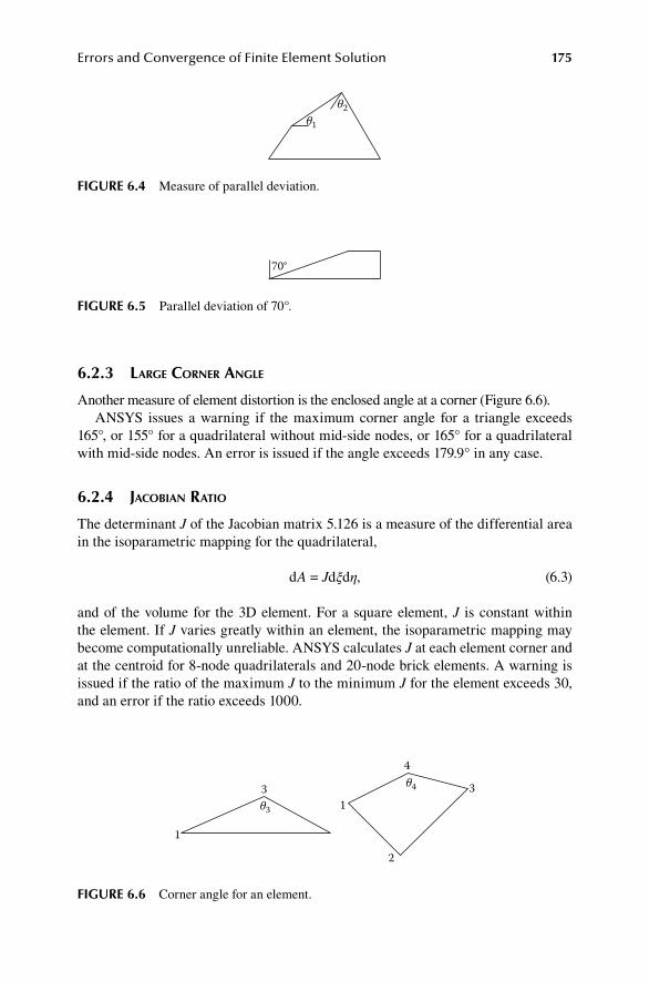
Errors and Convergence of Finite Element Solution 175
6.2.3 large corner angle
Another measure of element distortion is the enclosed angle at a corner (Figure 6.6).ANSYS issues a warning if the maximum corner angle for a triangle exceeds
165°, or 155° for a quadrilateral without mid-side nodes, or 165° for a quadrilateral with mid-side nodes. An error is issued if the angle exceeds 179.9° in any case.
6.2.4 JacoBian ratio
The determinant J of the Jacobian matrix 5.126 is a measure of the differential area in the isoparametric mapping for the quadrilateral,
dA = Jdξdη, (6.3)
and of the volume for the 3D element. For a square element, J is constant within the element. If J varies greatly within an element, the isoparametric mapping may become computationally unreliable. ANSYS calculates J at each element corner and at the centroid for 8-node quadrilaterals and 20-node brick elements. A warning is issued if the ratio of the maximum J to the minimum J for the element exceeds 30, and an error if the ratio exceeds 1000.
θ2θ1
fIgure 6.4 Measure of parallel deviation.
70°
fIgure 6.5 Parallel deviation of 70°.
3
1
θ3
θ4 3
4
2
1
fIgure 6.6 Corner angle for an element.

176 The Finite Element Method for Mechanics of Solids with ANSYS Applications
6.3 patch teSt
It is generally thought that convergence to the correct answer will occur if every patch of elements correctly models a constant strain condition. This is called the patch test, and should be applied to any element before using it.3
Consider any collection of contiguous elements, called a patch. Let ui ij ijc c c, , ,ε τ
denote the fields of displacement, strain, and stress for a case of constant strain. We can calculate the nodal displacements DK
c for the constant strain field from uic by
substituting the nodal coordinates. The nodal forces for the finite element of an analysis can be calculated in two
ways. First, using the stiffness matrix and the given nodal displacements DKc , we find
the corresponding nodal forces:
F = KDc. (6.4)
Second, we can calculate the nodal forces that correspond to the boundary trac-tions Ti
c, which are in equilibrium with the stress field τ ijc. Using the tractions Ti
c, the applied nodal forces should be:
F T N AK i iK
nTn
c c d= ∫∑S
.
(6.5)
If the patch of elements correctly models the state of constant strain, the two calcula-tions of nodal force must yield the same result: F = Fc.
There are other equivalent forms of the patch test. One can specify the displacements only on the edge of the patch and calculate the nodal displacement at interior nodes, where F = 0, and see if the interior nodes have displacements matching those gener-ated by ui
c. Alternatively, one could specify the nodal forces by F = Fc and use the finite element equations to calculate D, which is then compared to Dc. This last procedure is often easier, since the finite element code is always programmed to accept loads as input. Naturally, one has to impose displacement boundary conditions that are sufficient to pre-vent rigid motion in order to solve the equations when the forces are given.
The patch test can be carried out by actually doing the calculations on the computer, or we can investigate the formulation of the problem to predict the result in the following way. The finite element equation is derived from the virtual work relation:
τ εij ij i i i iV T u A b u V
n Tn n
d d dV S V∫∑ ∫∑ ∫∑= +0 , (6.6)
for every set of virtual nodal displacements DI, with εij and ui generated by the shape functions:
u N D e A Di iI I ij ijI
II
I= = ∑∑ , . (6.7)

Errors and Convergence of Finite Element Solution 177
For a constant strain field, bi = 0 and T Ti i= c , so the right-hand side of 6.4 is equal to F DK K
c∑ . The question now is whether the left-hand side gives that value for the chosen finite element model. The left-hand side of 6.6 can be integrated by parts over a region in which τ ij ju is continuous by using the virtual work formula. We wish to include the non-conforming elements in this analysis and, for them, ui is not continuous across element boundaries. Continuity will hold within each element so that, for each element, we have
τ ε τij ij i i ij j iV Tu A u V
m m m
d d dV V V∫ ∫ ∫= −
∂
, .
(6.8)
The integrals over the boundaries of the elements can be divided into the integral over the part that lies on the exterior boundary, if any, and the integral over the interior element boundary. Integrals over the common interior boundaries Snm of the elements n and m can then be combined to obtain the following result
τ εij ij
m
in
in
im
im
i iV T u T u A Tu A
m Tnm
d d dV SS∫∑ ∫∫∑= + + −( ) ττ ij j iu V, ,d
V∫
(6.9)
where we have used ui = 0 on any part Su of the exterior boundary. Given τ τij ij= c
and T Ti i= c, the last term is zero and the next to the last term is equal to FK Kcδ∑ .
Therefore,
τ δij ij
m
K KK
e V F
m
c cdV∫∑ ∑= ,
(6.10)
and the patch test is satisfied if the first term on the right-hand side is zero. That is,
( )T u T u Ain
in
im
im
nm
+ =∫∑ dS
0
(6.11)
is a necessary condition for satisfying the patch test.Let us next investigate this condition for conforming elements:
u u uin
im
i nm= = on S . (6.12)
In this case, the integrand of the term is zero if
T Tin
im
nm+ = 0 on S . (6.13)
Since the unit normals to the boundaries of adjacent elements are oppositely directed, this is the condition for equilibrium of tractions across element boundaries and is there-fore satisfied when τ τij ij= c . The conforming elements will therefore pass the patch test.

178 The Finite Element Method for Mechanics of Solids with ANSYS Applications
We see that 6.11 reduces to the condition for equilibrium of tractions at ele-ment boundaries if the displacements are continuous across the element bound-aries. However, this reduction does not occur if the displacements are not continuous across the element boundary as is the case for nonconforming elements, and the term may not be zero for the constant strain state. We must explicitly evaluate this term.
If every element is given the stress and strain associated with a constant strain field, the differential equations of equilibrium and the stress boundary conditions will be satis-fied, and the tractions Ti are constant for a given plane surface, having the same value for every element. Thus, if the element boundaries are plane, the integrals in 6.11 reduce to
( ) ( ) .T u T u A T u u Ain
in
im
im
in
in
im
nm nm
+ = −∑∫ ∫d d
S
(6.14)
Hence, the term will be zero if
( )u u Ain
im
nm
− =∫ dS
0
(6.15)
for every interior element boundary. This integral has to be investigated for a non-conforming element.
Even if 6.15 is not exactly satisfied, the finite element solution may still converge to the correct solution if the integrals tend to zero with the size of the element. Of course, the terms must be zero for the actual loading, not just for constant strain. However, as the element size tends to zero, the actual state of strain can be approxi-mated locally by a constant strain. Therefore, the test of a patch of elements in con-stant strain is thought to be a sufficient test for convergence.
6.3.1 wilSon–taylor quadrilateral
Let us consider, for example, the element discussed in Section 5.2.1—a rectangle with four nodeless parameters d.4 If the nodeless parameters are nonzero for an isoparametric element, the displacements are not linear along an edge and continuity is lost. However, if d is zero in a particular case, then continuity is achieved. For each element, d is given by 5.46. Hence, d is zero if
k D B CAD21 0= =∫∫ T dA .
(6.16)
For the patch test, the nodal coordinates D are given the values such that AD is a matrix of constant strain. Since CAD is then a matrix of constant stress, it can be factored outside the integral sign and d will be zero if
B BT Td d dA J∫∫ ∫∫= =ξ η 0.
(6.17)

Errors and Convergence of Finite Element Solution 179
For the rectangle, matrix B is given by 5.42 and contains only terms that are to the first power in ξ or η. Consequently, the integral 6.17 is indeed zero in this case. The displacement field is therefore continuous and the patch test will be satisfied.
If the shape functions are used to generate an isoparametric quadrilateral follow-ing the methods discussed in Section 5.5 with exact integration, the patch test fails unless the element is a parallelogram. However, it is possible to select the method of numerical integration so as to make d = 0 for a constant strain field. For the general case, 5.37 has the form
u N D N dk k
k
a
a
aα α α= += =
∑ ∑1
4
1
4ext
(6.18)
where
N N
N N
11 212
12 222
1
1
ext ext
ext ext
= = −
= = −
ξ
η
,
,
(6.19)
and
εαβ αβ αβ= += =
∑ ∑A D B dk k
k
a a
a1
8
1
4
,
(6.20)
where
JBJ N
x
N
x
J N
aa a
a
αβα
β
β
α
α
ξ
= ∂∂
+∂
∂
= ∂∂
2
2
ext ext
ext
θθ
θ
β
β
θ
θ
α
α
θθ
ξξ
ξ
ξ
∂∂
+∂
∂∂∂
= ∂∂
x
N
x
NJJ
a
a
ext
ext12 ββ
β
θθαξ
* *+∂
∂
NJJa
ext
,
(6.21)
∂∂
= ∂∂
=N a N11
1
11
220
ext ext
etcξ
ξξ
, , .
(6.22)
The terms ∂ ∂N aα θξext / are linear in (ξ,η), as are the terms JJθβ* . Their product is qua-
dratic and therefore the integral of B over the area of the element may not be zero.

180 The Finite Element Method for Mechanics of Solids with ANSYS Applications
For the Wilson–Taylor element, the Jacobean terms JJθβ* are evaluated at the cen-
troid and are therefore constant. The components of JB are then homogeneous linear functions of (ξ,η). The integral 6.17 will then integrate to zero and the patch test is satis fied. This modification is made in integration of all auxiliary matrices (5.44).
referenceS
1. Strang, G., and G. J. Fix, An Analysis of the Finite Element Method, Prentice-Hall, Englewood Cliffs, NJ, 1973.
2. ANSYS Theory Reference Manual, Section 13.7. 3. Bazeley, G. P., Y. K. Cheung, B. M. Irons, and O. C. Zienkiewicz, Triangular elements
in plate bending–conforming and nonconforming solutions, Proceedings of the First Conference on Matrix Methods in Structural Mechanics, Wright-Patterson AFB, Ohio, 1965. See also Irons, B. M., E. A. de Oliveira, and O. C. Zienkiewicz, Comments on the paper: Theoretical foundations of the finite element method, by Int. J. Solids Struct., 6, 695–697, 1970.
4. Taylor, R. L., P. J. Beresford, and E. L. Wilson, A non-conforming element for stress analysis, Int. J. Numer. Meth. Eng., 10, 1211–1219, 1976.

181
7 Heat Conduction in Elastic Solids
7.1 dIfferentIal equatIonS and vIrtual Work
In this chapter, we will only consider small deformations and small temperature changes. Let T denote the change in temperature of a material particle from a reference tempera-ture T0. That is, the absolute temperature of the particle is T + T0. For an elastic material with small temperature change, the stress–strain relation in matrix form is*
ττ εε ββ
εε ττ αα
ββ αα
= −
= +
=
−
C
C
C
T
T
,
,
.
1
(7.1)
α is the matrix of coefficients of linear expansion for the material. For an isotropic material αT = α[1 1 1 0 0 0] and β = β[1 1 1 0 0 0], β = (2μ + 3λ)α. The balance of energy provides the equation governing heart conduction at a material particle†
ρ ρc
T
tT r T
t
∂∂
= ∇ ∇ + − ∂∂
T Tκκ ββ εε0
(7.2)
where c is the specific heat at constant strain, κ is the matrix of thermal conductivi-ties, ρ is the mass density, and r is the energy supply at the element per unit mass. For an isotropic material, κij = κδij.
The gradient operator ∇ is a column matrix. In rectangular Cartesian coordinates,
∇ = ∂∂
∂∂
∂∂
T
x y z.
(7.3)
In cylindrical coordinates,
∇ = ∂∂
∂∂
∂∂
T
r r z
1θ
. (7.4)
* Dill: Section 2.10. Refer to Preface.† Dill: Equation 2.10.17. Refer to Preface.

182 The Finite Element Method for Mechanics of Solids with ANSYS Applications
The equivalent virtual work formula is generated by multiplying 7.2 by arbitrary functions T (i.e., a virtual temperature variation δT T= ), integrating over the vol-ume, and applying integration by parts to obtain
ρcTTt
V T T V T Tt
V Tq AV V V S
∂∂
+ ∇ ∇ + ∂∂
= − +∫ ∫ ∫ ∫d d d dT T( ) κκ ββ εε0 TT r V
V
ρ d∫ ,
(7.5)
where
q = –nTκ∇T (7.6)
is the heat flux into the body across the surface with outward normal n.After dividing the volume into finite elements, we introduce shape functions for
each element:
u = ND, ε = AD, T = ST, ∇T = BT, (7.7)
where T is the column matrix of nodal temperatures. Using the same shape functions to generate the virtual temperature variations yields the finite element form of the virtual work:
C T K T Q C Dtt tt tu + = − , (7.8)
where
K B Btt
V
V= ∫∑ T
elements
dκκ , (7.9)
C S Stt
V
c V= ∫∑ ρ T
elements
d , (7.10)
C S Atu
V
T V= ∫∑ 0T T
elements
dββ , (7.11)
Q S S= − +∫∑ ∫∑T
elements
T
elements
d dq A r VS V
ρ .
(7.12)
In the last equation, the surface integral includes only those segments of the surface that lie on the exterior boundary. Boundary conditions may provide nodal values of temperature T, or the given surface heat transfer q = qini. If the heat transfer at the surface is by convective exchange with a surrounding fluid, then
q = –h(Tf – T), (7.13)

Heat Conduction in Elastic Solids 183
where h is the film coefficient and Tf is the temperature of the fluid above the ref-erence temperature of the element. The surface integral in 7.12 then includes the unknown nodal temperatures:
S K T S
K S
T
elements
T
elements
q A h T A
h
S
tc
S
tc
d df∫∑ ∫∑= −
=
,
TT
elements
dS AS∫∑ .
(7.14)
The matrix Ktc can be added to the matrix Ktt.The complete heat conduction equations are coupled to the equations for the dis-
placements by the last term in 7.8. The displacement equations are coupled to the temperature equations by the thermal stress τ = –βT in 7.1, which contributes inter-nal nodal forces Fth according to 3.33. The mechanical equations including inertial and thermal forces are then
MD C D K D F F + + = −uu uu th , (7.15)
where
F K T
K A S
th ut
ut
V
V
=
= − ∫∑,
.T
elements
dββ
(7.16)
The coupled equations, 7.8 and 7.15, are
M DT
CC C
DT
00 0
0
+
uu
tu tt
+
=
K KK
DT
FQ
uu ut
tt0.
(7.17)
They must be solved simultaneously or by iteration. ANSYS provides elements SOLID5, PLANE13, AND SOLID98 for analysis of the transient thermoelastic coupled equations.
However, the coupling can often be neglected. Consider, for example, an isotropic material with constant κ so that the heat conduction equation (7.2) without radiation becomes
ρ κ µ λ αε
cT
tT T
tkk∂
∂= ∇ − + ∂
∂2
0 2 3( ) . (7.18)

184 The Finite Element Method for Mechanics of Solids with ANSYS Applications
Suppose that the body expands freely (τ = 0), the stress–strain relation 7.1 gives εkk = 3αT, and the heat conduction equation becomes
1
2 3 3
2
02
+( ) ∂∂
= ∇
= +
fT
t cT
fT
c
κρ
µ λ αρ
,
( ).
(7.19)
The nondimensional factor f is small for engineering materials. For a steel with
ρ = 8030 kg/m3, c = 503 J/kg °K,
α = 17.82 × 10⁻⁶/°K, κ = 16.3 J/s m °K,
E = 193 GPa, ν = 0.29, T0 = 293°K,
we find that f = 0.03. Consequently, the coupling of the equations through the strain in 7.2 can be neglected. The uncoupled equations can then be solved separately.
The temperature is first determined by the heat conduction equation:
C T K T Qtt tt + = . (7.20)
The deformations are then subsequently determined by the thermoelastic equations:
MD C D K D F F + + = −uu uu th. (7.21)
ANSYS provides elements Plane55, Plane 77, Solid70, and Solid90 for the tempera-ture calculations. The temperatures are saved for later stress analysis by
Load Step Options > Solution Printout,
which creates a file, jobname.rth. After the temperature analysis, the elements are switched to matching structural elements Plane 182, Plane 183, Solid185, or Solid186 for the thermal-stress analysis by the ETCHG command or
Element Type > Switch Element Type > Thermal to Structural.
The temperature is read into the displacement formulation by the LDREAD com-mand or
Define Loads > Apply > Structural > Temperature > From Thermal Analysis.
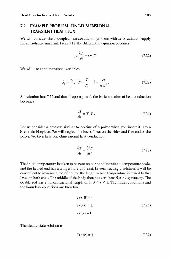
Heat Conduction in Elastic Solids 185
7.2 exaMple proBleM: one-dIMenSIonal tranSIent heat flux
We will consider the uncoupled heat conduction problem with zero radiation supply for an isotropic material. From 7.18, the differential equation becomes
ρ κc
T
tT
∂∂
= ∇2
(7.22)
We will use nondimensional variables:
ˆ , ˆ , ˆ .x
x
aT
T
Tt
t
cai
i= = =0
2
κρ
(7.23)
Substitution into 7.22 and then dropping the ^, the basic equation of heat conduction becomes
∂∂
= ∇T
tT2 .
(7.24)
Let us consider a problem similar to heating of a poker when you insert it into a fire in the fireplace. We will neglect the loss of heat on the sides and free end of the poker. We then have one-dimensional heat conduction:
∂∂
= ∂∂
T
t
T
x
2
2.
(7.25)
The initial temperature is taken to be zero on our nondimensional temperature scale, and the heated end has a temperature of 1 unit. In constructing a solution, it will be convenient to imagine a rod of double the length whose temperature is raised to that level on both ends. The middle of the body then has zero heat flux by symmetry. The double rod has a nondimensional length of 1: 0 ≤ x ≤ 1. The initial conditions and the boundary conditions are therefore
T x
T t
T t
( , ) ,
( , ) ,
( , ) .
0 0
0 1
1 1
=
=
=
(7.26)
The steady-state solution is
T(x,∞) = 1. (7.27)

186 The Finite Element Method for Mechanics of Solids with ANSYS Applications
The transient part is
θ(x,t) = T(x,t) – 1. (7.28)
The equations to be solved are
∂∂
= ∂∂
= −
=
=
θ θ
θ
θ
θ
t x
x
t
t
2
2
0 1
0 0
1 0
,
( , ) ,
( , ) ,
( , ) .
(7.29)
The solution is easily determined by separation of variables to be
θ ππ( , ) sin( )x t t n xn
n
= − −∑22 2
eodd
. (7.30)
The temperature at the free end of the original poker (x = 0.5) is
T t tn
nn
n
n
12
14
2
1
2 2
, sin
= −
= −
−
−
∑ e
e
odd
π
ππ
22 2 41 1 2π
πt
nn
n
( ) .( )/− −∑odd
(7.31)
For the finite element analysis (see Section 15.30), the rod is represented as a plane rectangle of thickness 0.1 and unit length, meshed by 10 four-node thermal elements (QUAD 4 node 55). Nominal values of the nondimensional material properties are used: κ = 1, ρ = 1, and c = 1. The exponential function decays rapidly and the temperature reaches 99% of steady state after the nondimensional time is 0.5. A comparison of the exact solution from 7.31 with the numerical solution for ∆t = 0.01 is shown in Tables 7.1 and 7.2. Note that the temperature is actually ramped up in the first numerical step so the theoretical instant step change in temperature is only approximated. One could take a very short first step then continue with larger steps.
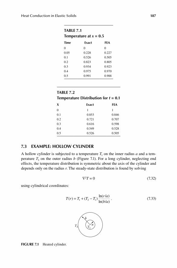
Heat Conduction in Elastic Solids 187
7.3 exaMple: holloW cylInder
A hollow cylinder is subjected to a temperature T1 on the inner radius a and a tem-perature T2 on the outer radius b (Figure 7.1). For a long cylinder, neglecting end effects, the temperature distribution is symmetric about the axis of the cylinder and depends only on the radius r. The steady-state distribution is found by solving
∇2T = 0 (7.32)
using cylindrical coordinates:
T r T T T
r a
b a( ) ( )
ln( )ln( )
= + −1 2 1
//
.
(7.33)
b
aT2 T1
fIgure 7.1 Heated cylinder.
taBle 7.2 temperature distribution for t = 0.1
x exact fea
0 1 1
0.1 0.853 0.846
0.2 0.721 0.707
0.3 0.616 0.598
0.4 0.549 0.528
0.5 0.526 0.505
taBle 7.1 temperature at x = 0.5
time exact fea
0 0 0
0.05 0.228 0.227
0.1 0.526 0.505
0.2 0.823 0.805
0.3 0.934 0.923
0.4 0.975 0.970
0.5 0.991 0.988
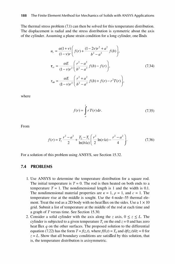
188 The Finite Element Method for Mechanics of Solids with ANSYS Applications
The thermal stress problem (7.1) can then be solved for this temperature distribution. The displacement is radial and the stress distribution is symmetric about the axis of the cylinder. Assuming a plane strain condition for a long cylinder, one finds
ur
f rr a
b af br = +
−+ − +
−
α ν
νν( )
( )( )
( )( ) ,
11
1 2 2 2
2 2
ττα
ν
τα
θθ
rr
E
r
r a
b af b f r
E
=−
−−
−
=
( )( ) ( ) ,
(
1 2
2 2
2 2
11 2
2 2
2 22
−+−
+ −
ν)( ) ( ) ( ) ,
r
r a
b af b f r r T r
(7.34)
where
f r r T r ra
r
( ) ( ) .= ∫ d
(7.35)
From
f r Tr a T T
b a
rr a
r a( )
ln( )ln( )= − + − − −
1
2 22 1
2 2 2
2 2 4//
.
(7.36)
For a solution of this problem using ANSYS, see Section 15.32.
7.4 proBleMS
1. Use ANSYS to determine the temperature distribution for a square rod. The initial temperature is T = 0. The rod is then heated on both ends to a temperature T = 1. The nondimensional length is 1 and the width is 0.1. The nondimensional material properties are κ = 1, ρ = 1, and c = 1. The temperature rise at the middle is sought. Use the 4-node–55 thermal ele-ment. Treat the rod as a 2D body with no heat flux on the sides. Use a 1 × 10 grid. Submit a list of temperature at the middle of the rod at each time and a graph of T versus time. See Section 15.30.
2. Consider a solid cylinder with the axis along the z axis, 0 ≤ z ≤ L. The cylinder is subjected to a given temperature T1 on the end z = 0 and has zero heat flux q on the other surfaces. The proposed solution to the differential equation (7.22) has the form T = f(z,t), where f(0,t) = T0 and ∂f(z,t)/∂z = 0 for z = L. Show that all boundary conditions are satisfied by this solution, that is, the temperature distribution is axisymmetric.

Heat Conduction in Elastic Solids 189
3. An unrestrained cylindrical rod with initial temperature T = 0 is heated on one end to a temperature T = 1. The nondimensional radius is 0.1, the non-dimensional length is 1, and the nondimensional material properties are E = 1, ν = 0.3, α = 1, κ = 1, ρ = 1, and c = 1. Heat loss on the exterior is neglected.(a) Determine the temperature distribution (0 ≤ t ≤ 1).(b) Determine the normal stress along the centerline at t = 0.4.
Use the four-node thermal element Plane 55 for transient temperature calculation. The Plane 182 element is then automatically used for the ther-mal stress. See Section 15.31.
4. Solve the problem described in Section 7.3 using the finite element method. Determine the maximum value of τθθ and the location, and compare the result with the exact solution from 7.34. Use actual dimensions and mate-rial properties: a = 5 in., T1 = 480°, T2 = 75°F, E = 2.9 × 10⁷ psi, ν = 0.3, ρ = 0.284 lb/in.3, α = 6.67 × 10⁻⁶/°F, κ = 8.092 × 10⁻⁴ BTU/in.2 °F, c = 0.1036 BTU/lb°F. Use ¼ of the disk with zero circumferential heat flux (Figure 7.2). See Section 15.32.
b
a
T1
T2
q =
0
q = 0
fIgure 7.2 Heated disk.


191
8 Finite Element Method for Plasticity
8.1 theory of plaStIcIty
The theory of plasticity describes the relation between load and deformation for many metals at higher stresses. The theory is rate independent: the same strains and stresses are obtained if the same loads are applied more rapidly (as long as inertial forces are negligible). The role of time in the constitutive equations is merely as a convenient bookkeeping parameter, and the occurrence of time derivatives does not indicate that such things as creep or relaxation can occur. The following is a sum-mary of the basic equations.*
The material is initially elastic:
τ ε ε τ( ) ( ) , ( ) ( ) .t c t t c tkm kmrs rs km kmrs rs= = −1
(8.1)
For an isotropic material,
cijkm = μ(δikδjm + δimδjk) + λδijδkm (8.2)
and
c
E Eijkm ik jm im jk ij km− = + + −1 1
2ν
δ δ δ δν
δ δ( ) .
(8.3)
When the stress—or equivalently, the strain—reaches a critical magnitude, the material yields and incremental deformations may be inelastic. If the magnitude of the stress then decreases, the incremental deformations are elastic. If the magnitude of the stress increases, the magnitude of the strain increases with apparently reduced moduli in a rate-independent manner. The additional strain,
ε ε τP( ) ( ) ( )t t c tij ij ijkm km= − −1
(8.4)
is called the plastic strain. Experiments on metals show that the volume change is elastic to a high degree of approximation, so that
εiiP = 0, (8.5)
* Dill: Chapter 4. Refer to Preface.

192 The Finite Element Method for Mechanics of Solids with ANSYS Applications
and we will consider only this case. Typical criteria for yielding have the form
f(τ(t),εP(t),β(t),κ(t)) ≤ 0 (8.6)
where the tensor β is called the back stress and the scalar κ is called the hardening parameter. Both parameters depend on the history of plastic strain. The yield func-tion f is normalized so that it is negative before yield, and yield occurs when f = 0. For fixed εP, β, and κ, the condition f = 0 defines a surface in stress space, which is called the yield surface. Experimental evidence shows that this surface is closed and convex, and we will also assume that it is smooth. The tensor
ητij
ij
f= ∂∂
(8.7)
is an outward normal to the yield surface. Suppose the material is at the point of yield so that f(t) = 0. An increment of stress inward from the yield surface reduces the magnitude of f and so an elastic increment in strain occurs. An increment in stress that is outward from the surface expands the yield surface and plastic strains occur. Let us define
f̂ ij ij= η τ .
(8.8)
At yield, f = 0, we have three possibilities:
(1) Elastic unloading: f̂ < 0 and therefore εεP = 0. (2) Plastic loading: f̂ > 0 and therefore εεP ≠ 0. (3) A neutral process: f̂ = 0 and εεP = 0.
For elastic unloading and the neutral process the incremental strain is elastic. Typical constitutive relations for the back stress and the hardening have the form
ββ == ττ εε ββ
== ττ
( ) ( ( ), ( ), ( ), ( )) ˆ( ),
( ) ( (
t t t t t f t
t k
b P κ
κ tt t t t f t), ( ), ( ), ( )) ˆ( ).εε ββP κ
(8.9)
The plastic strain increment during plastic loading is determined by
ε ηij ij
f
GP =
ˆ
2 (8.10)
where G is a plastic modulus that depends on the history of plastic straining. Using 8.4, we find for plastic loading that
ε η η τ( ) ( )t c
Gtij ijkm ij km km= +
−1 12 .
(8.11)

Finite Element Method for Plasticity 193
This equation can be inverted to obtain
τ εij ijkm kmc=
(8.12)
where the tangent modulus tensor is
c cg
c c
g G c
ijkm ijkm ijrs rs pq pqkm
ijrs i
= −
= +
12
2 2
µη η
µ η
,
jj rsη .
(8.13)
For an isotropic material,
c cg
g G
ijkm ijkm ij km
ij ij
= −
= +
2
2 2 2
µη η
µ µη η
,
.
(8.14)
A commonly used set of specific constitutive relations is the following
f t t t t t t
s sij i
( ( ), ( ), ( ), ( )) ( ) ( ),ττ εε ββP κ σ κ
σ
= −
= + 32 jj
ij ij
H
,
,
( ),
.
ββ == 0
23
κ ε
ε ε ε
=
= +
P
P P P
(8.15)
This is called the von Mises yield criterion with isotropic strain hardening, where σ is the effective stress, which is also called the von Mises stress, and ε P is the effective plastic strain. The tensor s is the deviatoric stress:
sij ij kk ij= −τ τ δ
13 .
(8.16)
In this case,
η
ση ηij
ijij ij
s= =3
232
, .and
(8.17)
From 8.8,
f̂
sij ij= 32
τσ .
(8.18)
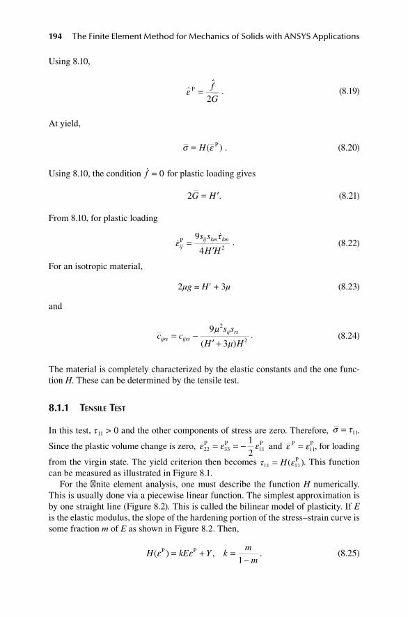
194 The Finite Element Method for Mechanics of Solids with ANSYS Applications
Using 8.10,
ε P = f̂
G2.
(8.19)
At yield,
σ ε= H( )P . (8.20)
Using 8.10, the condition f = 0 for plastic loading gives
2G H= ′. (8.21)
From 8.10, for plastic loading
ετ
ijij km kms s
H HP =
′9
4 2. (8.22)
For an isotropic material,
2μg = H′ + 3μ (8.23)
and
c c
s s
H Hijrs ijrs
ij rs= −′ +
9
3
2
2
µ
µ( ).
(8.24)
The material is completely characterized by the elastic constants and the one func-tion H. These can be determined by the tensile test.
8.1.1 tenSile teSt
In this test, τ11 > 0 and the other components of stress are zero. Therefore, σ τ= 11.
Since the plastic volume change is zero, ε ε ε22 33 11
12
P P P= = − and ε εP P= 11, for loading
from the virgin state. The yield criterion then becomes τ ε11 11= H( )P . This function can be measured as illustrated in Figure 8.1.
For the finite element analysis, one must describe the function H numerically. This is usually done via a piecewise linear function. The simplest approximation is by one straight line (Figure 8.2). This is called the bilinear model of plasticity. If E is the elastic modulus, the slope of the hardening portion of the stress–strain curve is some fraction m of E as shown in Figure 8.2. Then,
H kE Y km
m( ) , .ε εP P= + =
−1 (8.25)
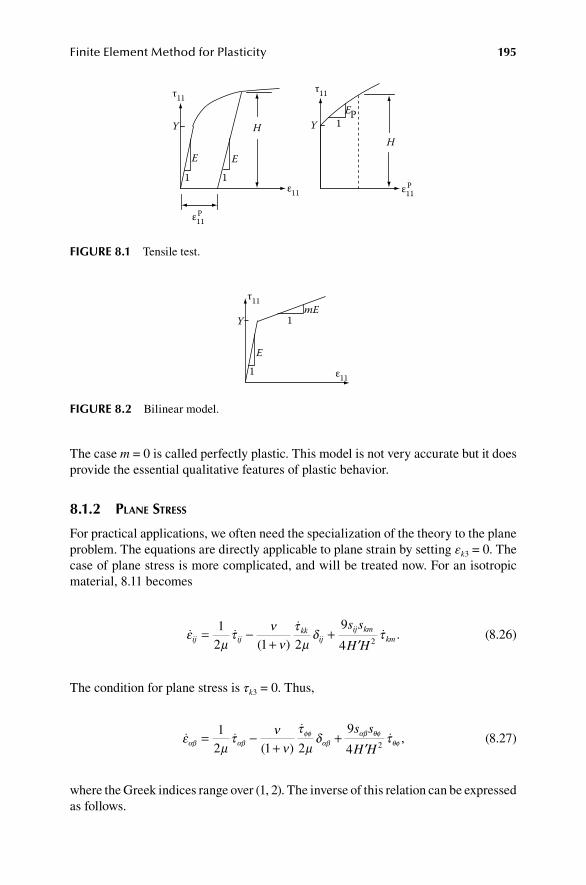
Finite Element Method for Plasticity 195
The case m = 0 is called perfectly plastic. This model is not very accurate but it does provide the essential qualitative features of plastic behavior.
8.1.2 plane StreSS
For practical applications, we often need the specialization of the theory to the plane problem. The equations are directly applicable to plane strain by setting εk3 = 0. The case of plane stress is more complicated, and will be treated now. For an isotropic material, 8.11 becomes
εµ
τν
ντ
µδ τij ij
kkij
ij kmkm
s s
H H= −
++
′1
2 1 2
9
4 2( ).
(8.26)
The condition for plane stress is τk3 = 0. Thus,
εµ
τν
ντ
µδ ταβ αβ
φφαβ
αβ θφθφ= −
++
′1
2 1 2
9
4 2( ),
s s
H H (8.27)
where the Greek indices range over (1, 2). The inverse of this relation can be expressed as follows.
YEP
1
HE E
Y
1 1
H
τ11τ11
Pε11
Pε11
ε11
fIgure 8.1 Tensile test.
ε11
E
Y
τ11mE
1
1
fIgure 8.2 Bilinear model.
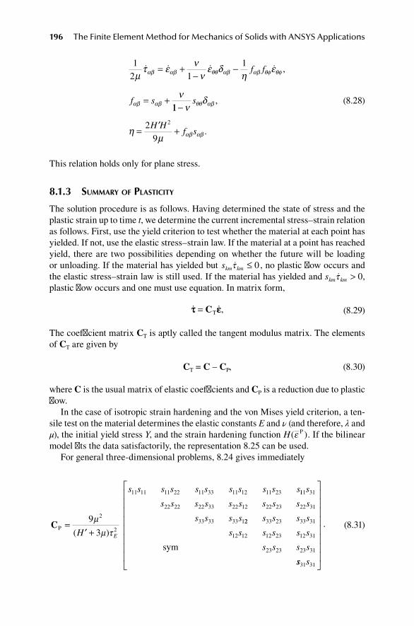
196 The Finite Element Method for Mechanics of Solids with ANSYS Applications
12 1
1µ
τ ε νν
ε δη
ε
ν
αβ αβ θθ αβ αβ θφ θφ
αβ αβ
= +−
−
= +
f f
f s
,
11
29
2
−
= ′ +
νδ
ηµ
θθ αβ
αβ αβ
s
H Hf s
,
.
(8.28)
This relation holds only for plane stress.
8.1.3 SuMMary of plaSticity
The solution procedure is as follows. Having determined the state of stress and the plastic strain up to time t, we determine the current incremental stress–strain relation as follows. First, use the yield criterion to test whether the material at each point has yielded. If not, use the elastic stress–strain law. If the material at a point has reached yield, there are two possibilities depending on whether the future will be loading or unloading. If the material has yielded but skm kmτ ≤ 0 , no plastic flow occurs and the elastic stress–strain law is still used. If the material has yielded and skm kmτ > 0, plastic flow occurs and one must use equation. In matrix form,
ττ εε= CT , (8.29)
The coefficient matrix CT is aptly called the tangent modulus matrix. The elements of CT are given by
CT = C – CP, (8.30)
where C is the usual matrix of elastic coefficients and CP is a reduction due to plastic flow.
In the case of isotropic strain hardening and the von Mises yield criterion, a ten-sile test on the material determines the elastic constants E and ν (and therefore, λ and μ), the initial yield stress Y, and the strain hardening function H( )ε P . If the bilinear model fits the data satisfactorily, the representation 8.25 can be used.
For general three-dimensional problems, 8.24 gives immediately
CP =′ +9
3
2
2
11 11 11 22 11 33 11 12 11 23
µµ τ( )H
s s s s s s s s s s s
E
111 31
22 22 22 33 22 12 22 23 22 31
33 33 33 1
s
s s s s s s s s s s
s s s s 22 33 23 33 31
12 12 12 23 12 31
23 23 23 31
s s s s
s s s s s s
s s s ssym
ss s31 31
.
(8.31)

Finite Element Method for Plasticity 197
In this case of plane strain, this formula reduces to
CP =′ +9
3
2
2
11 11 11 22 11 12
22 11 22 22
µµ τ( )H
s s s s s s
s s s s sE
222 12
12 11 12 22 12 12
s
s s s s s s
.
(8.32)
For plane stress, from (8.1.28),
CP = 211 11 11 22 11 12
22 11 22 22 22 12
12 1
µη
f f f f f f
f f f f f f
f f 11 12 22 12 12f f f f
.
(8.33)
The plastic modulus CP = 0 if the stress level is below yield. Once yielding occurs, CP depends on the history of plastic strain. The constitutive relation determines only the rate of change in stress, so one must integrate over the history to obtain the total stress. In practice, we only know the direction of the external loads at time t. We may not know whether loading or unloading will occur for every point of the body. It is often necessary to proceed by trial and error: make an assumption at each point of loading or unloading, do the calculations of the incremental stress, and check to see if the assumption was correct.
8.2 fInIte eleMent forMulatIon for plaStIcIty
The fundamental problem is to find the displacement field such that the stress deter-mined by the constitutive relations will satisfy the equations of equilibrium and the load conditions at all times. We will proceed step by step to trace the history of deformation for a given sequence of loads. We will use matrix notation.
The displacement field within each element is described with the aid of shape functions in the same way as for elasticity:
u = ND. (8.34)
The strain field is still determined by the gradient of displacement so that
ε = AD. (8.35)
The shape functions N and the geometric matrix A are characteristics of the finite element model and are independent of the history of deformation.
The theorem of minimum potential energy does not apply in the theory of plas-ticity because of the path-dependent nature of the constitutive relations. However, the theorem of virtual work does apply since that theorem is independent of the constitutive assumption. The governing equations for the rate of displacement are

198 The Finite Element Method for Mechanics of Solids with ANSYS Applications
easily found by direct use of the virtual work formula. In matrix notation, with S the boundary of V,
εε ττT T T dd dV A VV S V∫ ∫ ∫= +u T u b .
(8.36)
This relation must hold for every compatible system of displacements u and strains εε. Compatible systems can be generated by using relations 8.34 and 8.35 where the nodal displacements are given arbitrary values: u ND= and εε = AD. Substituting these relations in 8.36 and requiring that the equation holds for arbitrary nodal dis-placements D gives the following simple balance of forces for the finite element model:
f = F, (8.37)
where
F N T N b= +∫∑ ∫∑T Td dA V
n nn nS V
, (8.38)
and
f A= ∫∑ T dττ V
nn V
.
(8.39)
The force matrix F is the matrix of nodal loads (and reactions) at any instant cal-culated from the surface tractions and body force in the usual manner: The surface integral extends over that part of the element that forms the exterior boundary, if any. Matrix f is the matrix of resisting nodal forces due to the internal stress state. Equation 8.37 merely states that the internal nodal forces balance the external nodal forces when the stresses are in equilibrium. The only time-dependent quantities in the formulas for f and F are the stress τ, the tractions T and possibly the body force b.
8.2.1 fundaMental Solution
The balance of forces (8.37) holds at every instant, but a direct solution is not pos-sible because we do not have a constitutive relation for the total stress. The constitu-tive relation for plasticity only determines the rate of stress:
ττ εε= CT . (8.40)
It is necessary to proceed step by step in time to trace the history of deformation. This is unavoidable whenever we have inelastic or nonlinear material behavior.

Finite Element Method for Plasticity 199
If the displacements and stresses are known at time tn, the solution can be marched forward by the approximation
D(tn+1) = D(tn) + D(tn)dt (8.41)
ττ ττ ττ( ) ( ) ( ) ,t t t tn n n+ = +1 d (8.42)
where dt = tn+1 – tn. Therefore, we proceed to develop a solution procedure for deter-mining the increments. The basic relation governing the increments is just the time derivative of the balance of forces (8.37). The value of F is the given time rate of loading. The value of f is found via the time derivative of 8.39 with ττ given by 8.40 and εε determined via the time derivative of 8.35 for each element. The result is f K D= T . Thus,
K DT = F , (8.43)
where the stiffness matrix is the merge of the element matrices given by
K A C ATT
T d= ∫V
V .
(8.44)
These element stiffness matrices depend on the history of strain through the tangent modulus CT. In the case of plane stress or plane strain, the volume integral reduces to the integral over the area.
This step-by-step solution can be made as accurate as desired by decreasing the step size (up to the limit imposed by the finite element idealization and the numeri-cal errors). However, each step requires that the stiffness matrix be reformed and the equilibrium equations 8.43 must be solved.
In this fundamental procedure, CP is corrected only at the end of each step, and the elements that yield in that step will have been assigned a stiffness that is too large (or too small for unloading). The error accumulates with each step and the final solu-tion will have a significant error unless the error in each time step is very small. One either has to use a very large number of time steps (very small increment in load) or else the solution for each step has to be improved over the accuracy obtained with the simple formula, 8.41.
8.2.2 iteration to iMproVe the Solution
The accuracy of each step can be improved, and therefore the need for small steps reduced, by iteration within each step. The general idea is an extension of the Newton–Raphson method of solution of a nonlinear algebraic equation. For any increments in stress and strain, to first order, we have
dτ = CTdε. (8.45)

200 The Finite Element Method for Mechanics of Solids with ANSYS Applications
Suppose that some approximation Di to the solution up to a particular time t has been found. We now wish to improve the solution by finding improved displacements Di+1 = Di + dDi. For the increment dDi in nodal displacements, the strains in an ele-ment will be changed according to formula 8.35,
dεi = AdDi, (8.46)
and the stress will be changed by 8.45. Thus,
d d dT Tττ εεi i i i i= =C C A D , (8.47)
where the tangent modulus is evaluated for the stress τi corresponding to the defor-mation history up to Di. The internal node forces for the ith iteration are given by 8.39 using the stress τi. The change in internal node forces for the i and i + 1 approxi-mations is therefore
d d dTf f f Ai i i i V
n
= − =+ ∫∑1 ττV
.
(8.48)
After calculating the internal nodal forces f i for the ith iteration, we seek a correc-tion such that the internal node forces f i+1 are equal to the applied loads F. Using 8.47, we see that the right-hand side of 8.48 is the tangent stiffness matrix times the incremental displacements. Thus,
K D F fTdi i i= − . (8.49)
The superscript i means that the term is evaluated for the ith iteration. The right-hand side is the unbalanced node force. F is the total applied load at the instant for which the iteration is taking place. The internal resisting node forces f i are given by
f AV
i i V
n
= ∫∑ T dττ .
(8.50)
The process is started by using the fundamental step-by-step process to generate a first approximation D1 for the displacements at time t + dt. Equation 8.49 is then solved for dD1 and so forth. The displacement
Di+1 = Di + dDi (8.51)
is an improved approximation.

Finite Element Method for Plasticity 201
Equation 8.49 describes the fundamental procedure. The stiffness matrix is reformed and the equilibrium equations are then solved at each iteration. One may, however, approximate KT
i by the tangent stiffness matrix for some particular time, say K KT T
i t= ( ), and keep it fixed throughout the iteration, or it may be corrected (updated) only after some fixed number of iterations. The process is a form of the modified Newton–Raphson method.
8.3 exaMple: Short BeaM
The plane stress problem examined in Section 2.1.14 and shown in Figure 8.3, will be solved for the case of the bilinear material model with the following material properties.
E = 30 × 103 ksi, ν = 1/3, Y = 30 ksi, k = 0.1
The four-node rectangle is used with 50 segments per side. That gives 2500 elements and 2601 nodes. In the actual analysis, the symmetry about the mid-plane x = 0.5 is used so that the actual number of elements is reduced by one-half (see Section 15.13).
In this problem, the singularity at the built-in corner means that the yield limit will be immediately exceeded at the corner for any nonzero load. However, the plas-tic zone is very localized for small loads. The finite element analysis for any finite number of elements gives a finite approximate solution for the maximum stress in the corner, and the calculated behavior is elastic until that stress reaches the yield point.
After an element reaches the yield stress, one must proceed step by step, or by iteration, for the subsequent loading. Up to five iterations were used in each subse-quent step, as needed to achieve the set error level. The calculated corner displace-ment is shown in Figure 8.4 for a monotonically increasing load.
As the load exceeds 5 ksi, increasing softening due to plastic flow can be seen. The corner element reaches the yield stress first, then the adjacent elements yield, and as the load increases the region of yielding grows outward from the corner. The
x
a
y ap
fIgure 8.3 Plane stress: short beam.

202 The Finite Element Method for Mechanics of Solids with ANSYS Applications
stresses at the integration points nearest the fixed boundary are shown in Figures 8.5 to 8.7 for the initial yield and two subsequent higher loads. The shoulder in the curve for σx occurs at the boundary of the yielded region. Since this material has nonzero strain hardening, the stress in the yielded region increases toward the boundary. However, the stresses in the yielded region grow more slowly because of the soften-ing of the yielded material. Very near the corner, the stress increases rapidly as it does near the singularity in the elasticity problem.
0 0.05
Stre
ss in
KSI
0.1 0.15 0.2
35
30
25
20
15
10
5
00.25
x0.3 0.35 0.4 0.45 0.5
τxy
σx
σy
fIgure 8.5 Short beam: stress at y = 0.004 for a load of 2.9 ksi.
Displacement × 1000
Shea
r loa
d (k
si)
14
12
10
8
6
4
2
00 1 2 3 4 5 6 7 8 9 10
fIgure 8.4 Plane stress example: short beam.

Finite Element Method for Plasticity 203
8.4 proBleMS
1. In a tensile test, τ11 = σ and the other stress components are zero. Show this for the case of loading of a material with a von Mises yield criterion and isotropic strain hardening.
2. For the bilinear plasticity model (Figure 8.8), show that the hardening law is
Stre
ss in
KSI
45
40
35
30
25
20
15
10
5
00 0.05 0.1 0.15 0.2 0.25
x0.3 0.35 0.4 0.45 0.5
τxy
σx
σy
fIgure 8.7 Short beam: stress at y = 0.004 for a load of 7 ksi.
Stre
ss in
KSI
40
35
30
25
20
15
10
5
00 0.05 0.1 0.15 0.2 0.25
x0.3 0.35 0.4 0.45 0.5
τxy
σx
σy
fIgure 8.6 Short beam: stress at y = 0.004 for a load of 5 ksi.

204 The Finite Element Method for Mechanics of Solids with ANSYS Applications
H kE Y k
m
m( ) , .ε εP P= + =
−1
3. Solve the plane stress problem shown in Figure 8.9 for an elastic–plastic material with von Mises yield and isotropic hardening with a bilinear model a = 1, p = 10,000, E = 30 × 106, ν = 1/3, Y = 30,000, ET = 2.727 × 10⁶. Use a 20 by 20 grid of 400 elements (see Section 15.13). Apply the load in 10 steps (0 ≤ t ≤ 1). Then remove the load (1 ≤ t ≤ 2). Submit:(a) A list of UX at the corner for each time step 0 ≤ t ≤ 2.(b) A plot of the normal stress along the base at maximum load (t = 1).(c) A plot of the residual normal stress along the base after unloading (t = 2).
Note: Be sure to adjust the colors to get a white background on your graphs. 4. Consider small deformations of a nonlinearly elastic material: τ = f(ε). Derive
the finite element equations for solution of the small displacement equations by the iterative procedure for a general element and shape functions.
5. Consider small deformations of a material such that τij = aijkmεkm + bijkmrsεkmεrs. Derive a solution procedure by the finite element method for a general ele-ment and shape functions.
BIBlIography
Khan, A. S., and Huang, S., Continuum Theory of Plasticity, John Wiley & Sons, New York, 1995.
Lubliner, J., Plasticity Theory, Macmillan Publ. Co., New York, 1990.Lubarda, V. A., Elastoplasticity Theory, CRC Press, New York, 2002.
x
a
y ap
fIgure 8.9 Short beam.
ε11
E
Y
τ11mE
1
1
fIgure 8.8 Bilinear model.

205
9 Viscoelasticity
9.1 theory of lInear vIScoelaStIcIty
Elastic materials are those for which stress is proportional to strain. A typical exam-ple of elastic behavior is provided by the ideal spring for which force (stress) is pro-portional to displacement (strain). The ideal spring can be used to model the general behavior of elastic materials in the following manner.
We have seen that an isotropic material is completely characterized by separately giving the constitutive law for volumetric strain and for distortion. For a linear elastic isotropic material, from 2.18,
skm = μ2ekm, (9.1)
13
τ κεkk kk= ,
(9.2)
where
κ λ µ= + 2
3.
(9.3)
These relations can also be obtained by applying the spring model (Figure 9.1) to each mode of deformation. The distortional strain is 2e and the corresponding spring constant is μ. The mean stress is τkk/3, the volumetric strain is εkk, and the spring constant for dilatation is κ. The two equations can then be combined by using the definition of the deviatoric components to obtain the single constitutive relation of the linear elastic isotropic material:
τkm = 2μεkm + λεiiδkm. (9.4)
Viscous fluids, on the other hand, have a part of the stress that is proportional to the rate of strain. A typical example of a mechanism exhibiting such behavior is the shock absorber or damper mechanism (Figure 9.2), for which force (stress) is propor-tional to velocity (strain rate).
When the distortion is modeled by a damper, we have in place of 9.1,
skm km= 2ηe , (9.5)
where η is called the shear viscosity.More complicated mechanical behavior is observed in polymers, metals at
higher temperatures, and other materials where simultaneous elastic and viscous
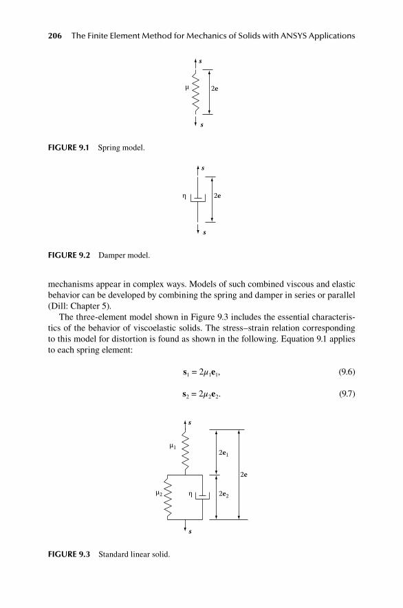
206 The Finite Element Method for Mechanics of Solids with ANSYS Applications
mechanisms appear in complex ways. Models of such combined viscous and elastic behavior can be developed by combining the spring and damper in series or parallel (Dill: Chapter 5).
The three-element model shown in Figure 9.3 includes the essential characteris-tics of the behavior of viscoelastic solids. The stress–strain relation corresponding to this model for distortion is found as shown in the following. Equation 9.1 applies to each spring element:
s1 = 2μ1e1, (9.6)
s2 = 2μ2e2. (9.7)
s
µ 2e
s
fIgure 9.1 Spring model.
s
2e
s
η
fIgure 9.2 Damper model.
2e1
2e2
2e
η
µ1
µ2
s
s
fIgure 9.3 Standard linear solid.

Viscoelasticity 207
Equation 9.5 applies to the damper:
s e3 32= η . (9.8)
The elements in parallel have a common strain and the total stress is the sum of that on each part:
e3 = e2, (9.9)
s2 + s3 = s. (9.10)
The units in series have a common stress and the total strain is the sum of that of each part:
s1 = s, (9.11)
e1 + e2 = e. (9.12)
The six quantities s1, s2, s3, e1, e2, and e3 are now eliminated from the seven equa-tions, 9.6–9.12, to obtain one stress–strain relation for distortion:
s s e e+ + = +µ µ
ηµ
µ µη
1 21
1 222
.
(9.13)
In addition to the model for distortion, the behavior in dilatation must also be speci-fied. Dilatation is often adequately modeled as elastic so that 9.2 applies. In this case, the complete set of constitutive equations comprises 9.2 and 9.13, which can be rewritten as follows:
τkk = 3κεkk, (9.14)
s e hkm km km= +2 1µ , (9.15)
where hkm is defined by
h e skm km km= − +2 1 2 1 2µ µ
ηµ µ
η.
(9.16)
Equations 9.14 and 9.15 yield the following constitutive relation for the three element model of distortion with elastic volume change:
τ µ ε λ ε δkm km ii km kmh= + +2 1 1 , (9.17)

208 The Finite Element Method for Mechanics of Solids with ANSYS Applications
where λ1 = κ – 2μ1/3. The material constants occurring in the constitutive relations can be determined by subjecting a rod to a uniaxial stress and measuring both the elongation and the lateral contraction. We will show below that 9.17 holds true for viscoelastic materials in general, but a general expression for hkm is needed.
A viscoelastic model based on an assembly of springs and dampers leads to a constitutive equation in the form of a differential equation such as 9.17. To determine the stress at time t for a given history of strain before time t, one must solve the dif-ferential equation. The order of the differential equation depends on the number of spring–damper elements to be used to construct the model, but in all cases one is led to a linear differential equation with constant coefficients. The form of the general solution to such an equation is known. For an isotropic material, the general form of the constitutive relation for a material that is unstrained up to t = 0 is
τ µ τ ε τ λ τ ε τ δ τkm km ii km
t
t t t( ) ( ) ( ) ( ) ( ) .= − + −{ }∫ 20
d
(9.18)
Note that we are using the letter τ as a dummy variable of integration and not to denote stress. The context should make the use clear.
The functions μ(t) and λ(t) are called the relaxation moduli and are determined by solving the differential equations provided by the model for a step change in strain at t = 0. These functions are given by
µ( ) e ,t A Anant
n
N
= + −
=∑0
1
(9.19)
κ
λ κ µ
( ) e ,
( ) ( ) ( ),
t B B
t t t
mbmt
m
M
= +
= −
−
=∑0
1
23
(9.20)
the so-called Prony or Dirichlet series. The constants A0, An, an, B0, Bn, and bn depend on the stiffness and viscosities of the spring–damper mechanisms. The number of exponential terms is equal to the number of dampers. In practice, the relaxation moduli are directly measured by experimental means for a particular material and the Prony series is numerically fitted to the data.
The constitutive equation 9.18 can be simplified by integration by parts. Note that
dd
dd
dd
ddτ
µ τµ
τµ
µ µ τ( ( ))( ) ( )
( ) ( )ss
s
s s
ss t= = − = − = − − ,,
(9.21)

Viscoelasticity 209
where s = t – τ. Note that we are using the letter s as a dummy variable of integration and not to denote stress s. Therefore,
ddτ
µ τ ε τ µ τ ε τ µ τ ε τ( ) ( ) ( ) ( ) ( ) ( ).t t t−{ } = − − −
(9.22)
Consequently, integration of 9.18 by parts yields
τ µ ε λ ε δ
µ τ ε τ
km km ii km
km
t t t
t
( ) ( ) ( ) ( ) ( )
( ) ( )
= +
+ −
2 0 0
2 dd dτ λ τ ε τ δ τ0 0
t
ii km
t
t∫ ∫+ −( ) ( ) ,
(9.23)
where we have used the initial conditions εkm(0) = 0.To determine a formula for the incremental stress, let us differentiate 9.23 with
respect to t. Recall that
dd
d dt
f t f t tf t
t
t t
( , ) ( , )( , )
.τ ττ
τ0 0∫ ∫= + ∂
∂
(9.24)
Thus, the general constitutive equation of an isotropic linearly viscoelastic material is
τ µ ε λ ε δkm km ii km kmt t t h( ) ( ) ( ) ( ) ( ) ,= + +2 0 0 (9.25)
where
h t t
t
km km ii km
km
= +
+ −
2 0 0
2
µ ε λ ε δ
µ τ ε τ
( ) ( ) ( ) ( )
( ) ( ) dd dτ λ τ ε τ δ τ0 0
t
ii km
t
t∫ ∫+ −( ) ( ) .
(9.26)
The general equation 9.25 has the same form as 9.17, but hkm is given by 9.26.One can see from 9.23 that stress is determined by the history of strain. The
essential computational difference between plasticity and viscoelasticity can be seen in the formulas for the rate of change in stress. In plasticity, the tangent modulus depends on the history of strain and the direction of the strain increment, but there is no memory term hkm. For viscoelasticity, the tangent modulus is constant but there is a memory term hkm(t).
From the point of view of the theory of material behavior, a viscoelastic material is one for which the stress has a memory of the history of strain, but it is a fading memory. Recent strain has a greater effect on current stress than events that occurred at an earlier time. The material exhibits creep and relaxation, and the stress required
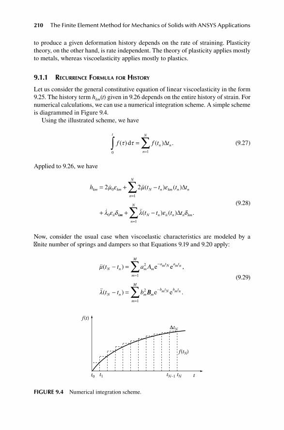
210 The Finite Element Method for Mechanics of Solids with ANSYS Applications
to produce a given deformation history depends on the rate of straining. Plasticity theory, on the other hand, is rate independent. The theory of plasticity applies mostly to metals, whereas viscoelasticity applies mostly to plastics.
9.1.1 recurrence forMula for hiStory
Let us consider the general constitutive equation of linear viscoelasticity in the form 9.25. The history term hkm(t) given in 9.26 depends on the entire history of strain. For numerical calculations, we can use a numerical integration scheme. A simple scheme is diagrammed in Figure 9.4.
Using the illustrated scheme, we have
f f t t
t
n n
n
N
( ) ( ) .τ τd0 1∫ ∑=
=
∆
(9.27)
Applied to 9.26, we have
h t t t tkm km N n km n n
n
N
ii k
= + −
+
=∑2 20
1
0
µ ε µ ε
λ ε δ
( ) ( )∆
mm N n ii n n km
n
N
t t t t+ −=
∑ λ ε δ( ) ( ) .∆1
(9.28)
Now, consider the usual case when viscoelastic characteristics are modeled by a finite number of springs and dampers so that Equations 9.19 and 9.20 apply:
µ
λ
( ) ,
( )
t t a A
t t b
N n m mamtN amtn
m
M
N n m
− =
− =
−
=∑ 2
1
2
e e
BBmbmtN bmtn
m
M
e e−
=∑
1
.
(9.29)
ttNtN–1t0 t1
f (tN)
f (t)
ΔtN
fIgure 9.4 Numerical integration scheme.

Viscoelasticity 211
Substituting these expressions into 9.28 gives
h a A
b B
km km p p kmp
p
M
ii km p p p km
= +
+ +
=∑2 0
2
1
02
µ ε α
λ ε δ β δpp
M
=∑
1
,
(9.30)
where, at time t = tN,
α ε
β
kmp
aptN aptn
n
N
km n n
p
bptN bptn
t t=
=
−
=
−
∑21
e
e e
e ( ) ,∆
nn
N
ii n nt t=
∑1
ε ( ) .∆
(9.31)
It follows from 9.31 that αkmp(tN) and βp(tN) may be calculated by the following recur-rence formulas.
α ε α
β ε
kmp N km N N
ap tNkmp N
p N
t t t t
t
( ) ( ) e ( ),
( )
= +
=
−−2 1∆
∆
iii N N
bp tNp Nt t t( ) ( ),∆
∆+
−−e β 1
(9.32)
with
α
β
kmp
p
( ) ,
( ) .
0 0
0 0
=
=
(9.33)
We have seen that the term hkm depends on the strains at all past times. However, it can now be seen from 9.30 to 9.33 that hkm can be calculated if the strain at the present time and the immediately previous values of αkmp and βp are saved in storage. Since the number of dampers M, which are needed to obtain a practical description of a material, will be much smaller than the number N of time steps, there is a con-siderable saving of computer memory for storage of history data.
9.1.2 ViScoelaStic exaMple
The plane strain problem shown in Figure 9.5 will be solved numerically. The con-stant load is applied suddenly at time t = 0. The three-element model shown in Figure 9.3 will be used for distortion and elastic volume change will be used to
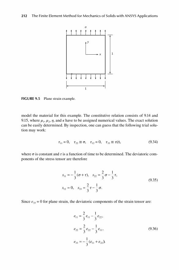
212 The Finite Element Method for Mechanics of Solids with ANSYS Applications
model the material for this example. The constitutive relation consists of 9.14 and 9.15, where μ1, μ2, η, and κ have to be assigned numerical values. The exact solution can be easily determined. By inspection, one can guess that the following trial solu-tion may work:
τ11 = 0, τ22 ≡ σ, τ12 = 0, τ33 ≡ τ(t), (9.34)
where σ is constant and τ is a function of time to be determined. The deviatoric com-ponents of the stress tensor are therefore
s s
s s
11 22
12 33
13
23
13
023
13
= − + = −
= = −
( ), ,
, .
σ τ σ τ
τ σ
(9.35)
Since ε33 = 0 for plane strain, the deviatoric components of the strain tensor are:
e
e
e
11 11 22
22 22 11
33 11 22
23
13
23
13
13
= −
= −
= − +
ε ε
ε ε
ε ε
,
,
( )).
(9.36)
1
1
y
x
σ
fIgure 9.5 Plane strain example.
Viscoelasticity 213
A constant ν = (3κ – 2μ1)/(2μ1 + 6κ) analogous to the Poisson ratio of elasticity can be introduced to obtain
τ
µ νν
εkk kk= +−
2 11 2
1( )( )
.
(9.37)
Since ε33 = 0, using 9.34, this relation becomes
ε εν
µ νσ τ11 22
1
1 22 1
+ = −+
+( )( )
( ). (9.38)
Next, set k and m equal to 3 in the constitutive relation 9.15 for distortion, obtaining
s e s e33 1 33
1 233
1 2332
2= − + +µµ µ
ηµ µ
η.
(9.39)
Using 9.35, 9.36, and 9.38, one finds for σ = 0 that
τ τ σ+ =A B , (9.40)
where
A = + +
13
2 1 31 2ηµ ν µ( ) ,
(9.41)
B = + +
13
1 31 2ηµ ν νµ( ) .
(9.42)
The solution of 9.40 is
τ τ σ σ( ) ( ) e .t
B
AAt B
A= −
+−0
(9.43)
Now, return to the relations 9.13, from which
s s s s e e11 22
1 222 11 1 11 22
1 222− = + − + − +µ µ
ηµ
µ µη
( ) ( ) (( ).e e11 22−
(9.44)
Using 9.35, 9.36, and 9.38 with σ = 0 , one finds
ε ε
µη
ε εµ µ
µ ησ11 22
211 22
1 2
12− + − = − +
( ) ,
(9.45)
214 The Finite Element Method for Mechanics of Solids with ANSYS Applications
The solution of this differential equation is
ε ε ε ε
µ µµ µ
σ µ η11 22 11 22
1 2
1 2
20 02
− = − + +
−−( ) ( ) e t / µµ µ
µ µσ1 2
1 22+
.
(9.46)
From 9.38 and 9.46,
εν
µ ντ
νν
µµ
σµ22
1
1
2 1
1 24 1
1 21
14
1
( )( )
t = −+
+ −+
+ +
−22
0 0211 221 2
1 2
2ε εµ µ
µ µσ µ η( ) ( ) e .− + +
− t /
(9.47)
The initial values of strain still have to be calculated. The load is applied suddenly, with a jump in stress at t = 0, but no jump in the strain of the damper is allowed. For the initial jump, 9.17 gives
τkm(0) = 2μ1εkm(0) + λ1εii(0)δkm, (9.48)
or, with ε33 = 0,
2μ1εαβ(0) = ταβ(0) – ντγγ(0)δαβ. (9.49)
Using 9.38, one finds
2 0
2 0 1
01 22
1 11
1 22
1
1
µ ε νσ
µ ε ν σ
τλ ν
µ
( ) ,
( ) ( ) ,
( )( )
= −
= −
= −σσ νσ= .
(9.50)
Using these values for the initial conditions, from 9.43,
τσ
α α ν β( )( ) e
t t= − − − ,
(9.51)
and from 9.47,
µ εσ
ν νν
νν
τσ
1 22 1 2 14 1
1 24 1
( ) ( )( )
( )( )
( ) (t k t= − + ++
+ −+
− 114
+ − −k tν)e , (9.52)
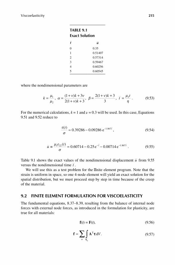
Viscoelasticity 215
where the nondimensional parameters are
k
k
k
kt
t= = + ++ +
= + + =µµ
αν ν
νβ
ν µη
1
2
21 32 1 3
2 1 33
,( )
( ),
( ), .
(9.53)
For the numerical calculations, k = 1 and ν = 0.3 will be used. In this case, Equations 9.51 and 9.52 reduce to
τσ( )
,t t= − −0 0.39286 .09286 e 1.867
(9.54)
u
t t t≡ = − −− −µ εσ
1 22 1 8670 60714 0 25 0 00714( )
. . e . e . . (9.55)
Table 9.1 shows the exact values of the nondimensional displacement u from 9.55 versus the nondimensional time t .
We will use this as a test problem for the finite element program. Note that the strain is uniform in space, so one 4-node element will yield an exact solution for the spatial distribution, but we must proceed step by step in time because of the creep of the material.
9.2 fInIte eleMent forMulatIon for vIScoelaStIcIty
The fundamental equations, 8.37–8.39, resulting from the balance of internal node forces with external node forces, as introduced in the formulation for plasticity, are true for all materials:
f (t) = F(t), (9.56)
f AV
= ∫∑ T dττ V
nn
.
(9.57)
taBle 9.1 exact Solution
t u
0 0.35
1 0.51407
2 0.57314
3 0.59467
4 0.60256
5 0.60545

216 The Finite Element Method for Mechanics of Solids with ANSYS Applications
F(t) is the matrix of given external node forces and reactions. The only difference in the formulation for various different materials is the constitutive relation for stress as a function of the history of strain. The constitutive equation (9.25) of a viscoelastic material, in matrix form, is
ττ εε= +C h, (9.58)
where τ, ε, and h denote column matrices, C is the matrix of instantaneous elasticity, and h is the memory term. For the plane problem,
ττ == εε ==τ
τ
τ
ε
ε
ε
11
22
12
11
22
122
,
=
, .h
h
h
h
11
22
12
(9.59)
The coefficient matrix C is the matrix of elastic constants with μ and λ replaced by μ(0) and λ(0), respectively. The matrix h is determined from 9.26 in general, or from 9.16 when the three-element model with elastic volume change is used. In the latter case,
h
h
h
e
e
e
11
22
12
1 2
11
22
12
2
=
µ µη
− +
µ µη
1 2
11
22
12
s
s
s
.
(9.60)
The elastic volume change 9.14 is used to find τ33 in plane strain or ε33 in the case of plane stress.
9.2.1 BaSic Step-By-Step Solution Method
From 8.35, 9.57, and 9.58,
f KD H( ) ( ) ( )t t t= + , (9.61)
where
K A CAV
= ∫∑ T dV
nn
(9.62)
is the stiffness matrix for the instantaneous elasticity, and
H A hV
( ) ( )t t V
nn
= ∫∑ T d
(9.63)

Viscoelasticity 217
is the memory load. The balance of external and internal nodal forces 9.56 leads to the equation for D as follows:
KD F H ( ) ( ) ( )t t t= − . (9.64)
Note that the stiffness matrix is constant for viscoelastic materials, but the right-hand side contains the memory load as well as the external nodal forces. We can now proceed in a step-by-step manner to construct the solution as a function of time. The fundamental procedure is to use the lower-order terms of the power series representation to march the solution forward. That is, having determined the solu-tion up to time tn, so that D(tn ) and τ(tn ) are known, the solution at time tn+1 is deter-mined by
D D D( ) ( ) ( ) ,t t t tn n n+ = +1 ∆ (9.65)
ττ ττ ττ( ) ( ) ( ) .t t t tn n n+ = +1 ∆ (9.66)
Any finite element code for thermoelastic stress analysis is easily extended to assem-ble and solve Equation 9.64. Note that K needs be formed and inverted only once. Equation 9.64 forms a set of linear ordinary differential equations in time. The solu-tion procedure can be improved by using the solution methods for dynamical prob-lems, which will be discussed in the next chapter.
9.2.2 Step-By-Step calculation with load correction
The basic step-by-step method can be improved if we take into account that f(tn ) is only approximately equal to F(tn ). The incremental load then consists of the memory load and the unbalanced node forces as follows. Having determined the solution up to time t, we seek the solution at time t + dt for which
f AV
( ) ( )t t t t V
nn
+ = +∫∑∆ ∆T dττ .
(9.67)
Writing τ(t + Δt) = τ(t) + Δτ, we have
f f AV
( ) ( ) .t t t V
nn
+ = + ∫∑∆ ∆T dττ
(9.68)
Since
Δτ = CΔε + hΔt (9.69)

218 The Finite Element Method for Mechanics of Solids with ANSYS Applications
and
Δε = AΔD, (9.70)
we have
f(t + Δt) = f(t) + KΔD + ΔH, (9.71)
where
∆ ∆H A h= ∫∑ T dt V
nn V
.
(9.72)
We seek a solution for which f (t + Δt) = F(t + Δt). Therefore, 9.71 becomes
KΔD(t) = F(t + Δt) – f(t) – ΔH(t). (9.73)
The finite element program is used to solve for ΔD and the solution is marched for-ward as before.
9.2.3 plane Strain exaMple
The example problem, for which the exact solution is given in Section 9.1.2, was solved using one 4-node square element. Since the strains are uniform in the exact solution, no approximation is introduced by the finite element idealization and one element provides an exact representation. The only error here is due to the numerical integration in time. The results using the basic step-by-step formula 9.64 are shown in Figure 9.6. As the exact solution 9.55 shows, the solution to this particular problem
∆t = 0.04∆t = 0.20∆t = 0.4
0 10.2 0.4 0.6 0.8 1.2 1.4 1.6 1.8 2Time
Disp
lace
men
t
0.65
0.6
0.55
0.5
0.45
0.4
0.35
fIgure 9.6 Basic step-by-step solution.
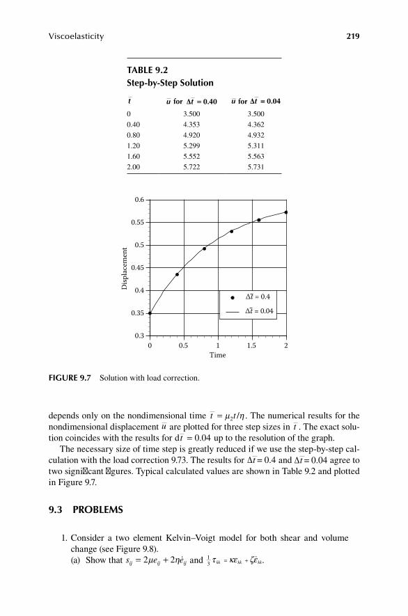
Viscoelasticity 219
depends only on the nondimensional time t t= µ η2 / . The numerical results for the nondimensional displacement u are plotted for three step sizes in t . The exact solu-tion coincides with the results for dt = 0 04. up to the resolution of the graph.
The necessary size of time step is greatly reduced if we use the step-by-step cal-culation with the load correction 9.73. The results for ∆t = 0.4 and ∆t = 0.04 agree to two significant figures. Typical calculated values are shown in Table 9.2 and plotted in Figure 9.7.
9.3 proBleMS
1. Consider a two element Kelvin–Voigt model for both shear and volume change (see Figure 9.8).(a) Show that s e eij ij ij= +2 2µ η and 13 τ κε ζεkk kk kk= + .
taBle 9.2 Step-by-Step Solution
t u for ∆t == 0.40 u for ∆t == 0.04
0 3.500 3.500
0.40 4.353 4.362
0.80 4.920 4.932
1.20 5.299 5.311
1.60 5.552 5.563
2.00 5.722 5.731
0 0.5 1 1.5 2
Disp
lace
men
t
Time
∆t = 0.4
∆t = 0.04
0.6
0.55
0.5
0.45
0.4
0.35
0.3
fIgure 9.7 Solution with load correction.

220 The Finite Element Method for Mechanics of Solids with ANSYS Applications
(b) Show that these equations are equivalent to the single constitutive
equation τ µε λε δ ηε λ ε δkm km ii km km ii km= + + +2 2 D where λ µ λ ζ η= − = −b23
23
, .D
λ µ λ ζ η= − = −b23
23
, .D
2. Given the standard linear solid model for distortion (Figure 9.3), determine the creep compliance.
Answer: 2 1 1 112
12 1 2 22
e t
st
( )exp( )= + − −
µ µ µ
µ η/
3. In matrix form, the constitutive relation for the Kelvin–Voigt material is ττ εε εε= +C CD .
Derive the finite element form of the equilibrium equations for this mate-rial model.
4. Determine the creep compliance for the tensile test of a material modeled by an elastic volume change and the three-element model in shear.
5. Analyze the creep test by the finite element method from the given relax-ation modulus and compare with the results of problem 5. See Section 15.14.
6. Solve the example illustrated in Figure 9.5 using ANSYS (see Section 15.15). Use G(0) = 100, G(∞) = 50, K(0) = K(∞) = 650/3. There is one dash-pot with G1 = G(0) – G(∞) and a relaxation time of 0.5. The load σ = 1 is constant (step) in time. Submit:(a) A list of UY at the corner for each time step 0 < t ≤ 3.(b) A plot of UY(t).
BIBlIography
Bland, D. R., The Theory of Linear Viscoelasticity, Pergamon Press, Oxford, England, 1960.Christensen, R. M., Theory of Viscoelasticity, 2nd ed., Academic Press, New York, 1982.Leitman, M. J., and G. M. Fisher, The linear theory of viscoelasticity, in Encyclopedia of
Physics, Vol. VIa/3, ed. S. Flügge, Springer-Verlag, New York, 1973.Lockett, F. J., Nonlinear Viscoelastic Solids, Academic Press, New York, 1972.
τkk13
τkk
εkk
13
ζb2e
s
ηµ
s
fIgure 9.8 Kelvin–Voigt model.

221
10 Dynamic Analyses
10.1 dynaMIcal equatIonS
In this section, we shall formulate finite element equations that include the inertial forces that have been neglected up to now.
10.1.1 luMped MaSS
The most direct way of discovering suitable equations governing motion is to con-centrate the total mass at node points and apply d’Alembert’s principle. Consider, for example, the solution of the plane problem using the rectangular elements (Section 5.1.4). A typical node arrangement is shown in Figure 10.1. The total mass of the material surrounding a node, shown by dashed lines, is treated as a point mass at that node.
Suppose the node spacing is uniformly “a by b” and the mass density of a unit slice of material is ρ. At an interior point, the lumped mass is ρab. At a corner the lumped mass is 1/4 ρab, and at a side point the lumped mass is 1/2 ρab. The effect of inertia is then to exert at each node a force “−mD”. At an interior node, for example, the x and y components of inertial force are ( , )− −ρ ρabU abV . For the entire body, the inertial forces have the form
F MDI = − , (10.1)
where M is a diagonal matrix continuing the list of lumped masses as shown in Figure 10.1. The complete equations of motion are then obtained from static formu-lation by adding these inertial forces to any applied external loads:
KD F MD= − , (10.2)
where F denotes the matrix of external loads. Recall that rigid translation and rotation are allowed by 10.2 if no boundary conditions on displacement have been imposed.
Equation 10.2 has the form of the usual dynamical equations of discrete systems. We may think of Equation 10.2 as representing N masses connected by “springs” and proceed to solve them in the usual fashion. From that point of view, the finite element procedure merely determines the effective spring constants.
In the lumped mass approach, the finite element idealization is not directly con-nected with the dynamical idealization, other than to indicate an appropriate set of points for the lumped masses. The distribution of mass between the nodes, as just described, is a rather arbitrary choice, but it has been found to work well in practice as long as all mass is accounted for. However, one can proceed in a more rational manner, as we shall now present.
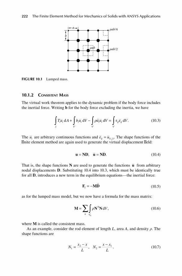
222 The Finite Element Method for Mechanics of Solids with ANSYS Applications
10.1.2 conSiStent MaSS
The virtual work theorem applies to the dynamic problem if the body force includes the inertial force. Writing b for the body force excluding the inertia, we have
Tu A b u V u u V Vi i i i i i ij ijd d d dS V V V∫ ∫ ∫ ∫+ − =ρ τ ε . (10.3)
The ui are arbitrary continuous functions and εij i ju= ( , ). The shape functions of the finite element method are again used to generate the virtual displacement field:
u ND u ND= =, . (10.4)
That is, the shape functions N are used to generate the functions u from arbitrary nodal displacements D. Substituting 10.4 into 10.3, which must be identically true for all D, introduces a new term in the equilibrium equations—the inertial force:
F MDI = − (10.5)
as for the lumped mass model, but we now have a formula for the mass matrix:
M N= ∫∑ ρ T dN VVn
n
,
(10.6)
where M is called the consistent mass.As an example, consider the rod element of length L, area A, and density ρ. The
shape functions are
N
x x
LN
x x
L12
21= − = −
, .
(10.7)
a
b
ρab/4
ρab/2ρab
fIgure 10.1 Lumped mass.

Dynamic Analyses 223
The consistent mass matrix is
M =
=
∫ ρ
ρN
NN N A x
AL
x
x
1
21 2
1
2
62 11 2
d .
(10.8)
Let us next consider the rectangular element described in Section 5.1. If we order the list of nodes by grouping all x components followed by all y components, DT = [UT,VT], the shape functions are
U V
N0
0=
= + +N
NN
k
k
k k k, ( )(14
1 1ξ ξ η η)) .
(10.9)
Using 10.6, one finds
U V
MM
M=
1
1
0
0,
(10.10)
where
M N N
N N
1
1
1
1
1
4
36
42 4
1 2
=
=
=
∫∫
∫∫−
+
−
+
T
T
d
d d
sym
ρ
ρ ζ
ρ
η
A
ab
ab
442 1 2 4
.
(10.11)
As a third example, let us consider the triangular element discussed in Section 4.2. Again, grouping the nodes by component, the shape functions from 4.16 are
N =
ζ ζ ζ
ζ ζ ζ1 2 3
1 2 3
0 0 0
0 0 0,
(10.12)
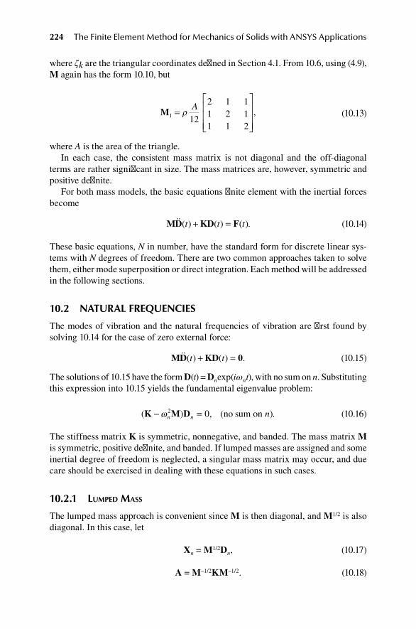
224 The Finite Element Method for Mechanics of Solids with ANSYS Applications
where ζk are the triangular coordinates defined in Section 4.1. From 10.6, using (4.9), M again has the form 10.10, but
M1 12
2 1 11 2 11 1 2
=
ρA
,
(10.13)
where A is the area of the triangle.In each case, the consistent mass matrix is not diagonal and the off-diagonal
terms are rather significant in size. The mass matrices are, however, symmetric and positive definite.
For both mass models, the basic equations finite element with the inertial forces become
MD KD F( ) ( ) ( ).t t t+ = (10.14)
These basic equations, N in number, have the standard form for discrete linear sys-tems with N degrees of freedom. There are two common approaches taken to solve them, either mode superposition or direct integration. Each method will be addressed in the following sections.
10.2 natural frequencIeS
The modes of vibration and the natural frequencies of vibration are first found by solving 10.14 for the case of zero external force:
MD KD 0( ) ( ) .t t+ = (10.15)
The solutions of 10.15 have the form D(t) = Dnexp(iωnt), with no sum on n. Substituting this expression into 10.15 yields the fundamental eigenvalue problem:
( ) , ( ).K M D− =ω n n n2 0 no sum on (10.16)
The stiffness matrix K is symmetric, nonnegative, and banded. The mass matrix M is symmetric, positive definite, and banded. If lumped masses are assigned and some inertial degree of freedom is neglected, a singular mass matrix may occur, and due care should be exercised in dealing with these equations in such cases.
10.2.1 luMped MaSS
The lumped mass approach is convenient since M is then diagonal, and M1/2 is also diagonal. In this case, let
Xn = M1/2Dn, (10.17)
A = M–1/2KM–1/2. (10.18)

Dynamic Analyses 225
The eigenvalue problem 10.16 becomes
( )A I X− =ω n n2 0, (10.19)
with A symmetric. This equation is a standard problem in numerical analysis, and many effective solution algorithms are available. Once solution vectors Xn are known, the mode shapes are calculated by 10.17: Dn = M–1/2Xn.
10.2.2 conSiStent MaSS
In the general case, when M is not a diagonal matrix but is symmetric positive defi-nite, we can proceed as follows in order to reduce the eigenvalue problem to the standard form. There exists triangular matrices L such that
M = LLT. (10.20)
The matrix L is easily inverted. There is a standard procedure for calculating L known as the Choleski decomposition. Now, define
A = L–1K(L–1)T, (10.21)
Xn = LTDn, (10.22)
and the standard eigenvalue problem 10.19 results.
10.3 Mode SuperpoSItIon SolutIon
It is now assumed that the N solutions of 10.16 have been found. The modal vectors satisfy the orthogonality conditions (n ≠ m):
(Dn)TKDm = 0, (10.23)
(Dn)TMDm = 0. (10.24)
The solution D(t) of the complete equations 10.15 can be expressed as a linear com-bination of the mode shapes:
D D T q
T q
( ) ( ) [ ]{ ( )},
[ ] [ ], { ( )} { (
t q t t
D t q t
n
n
n
in n
= =
= =
∑))},
(10.25)
where T is a square matrix whose columns are the mode shape vectors. Substituting 10.25 into 10.15, and using 10.23 and 10.24, one finds the set of uncoupled equations:

226 The Finite Element Method for Mechanics of Solids with ANSYS Applications
q q
P
Mnn n n
n
n
+ =ω 2 , ,no sum on
(10.26)
where
M
K M
P
n n n
n n n n n
n n
=
= =
=
( ) ,
( ) ,
( ) .
D MD
D KD
D F
T
T
T
ω 2
(10.27)
The modal equations 10.26 have the solution
qM
P tM
P tnn n
n n
t
n nn
t
= − = −∫ ∫1 1
0 0ω
τ ω τ τω
τ( ) sin ( ) (d )) sin .ω τ τn( ) d
(10.28)
If Pn is constant, that is, a step function at t = 0, then
q
P
Ktn
n
nn= −( cos( )).1 ω
(10.29)
If Pn is ramped up to a constant value as shown in Figure 10.2, then
q tP
K
t
t
t
tt tn
n
( )sin( )
, ,= −
≤ ≤0
1 110
ωω
(10.30)
q tP
K
t
tt t tn
n
( )sin( )
cos( ) , ,= −
≤0 1
111
2
2
ωω
ω/
/
(10.31)
where t t t= − 1 2/ .
t1
P0
Pn(t)
t
fIgure 10.2 Ramped load.
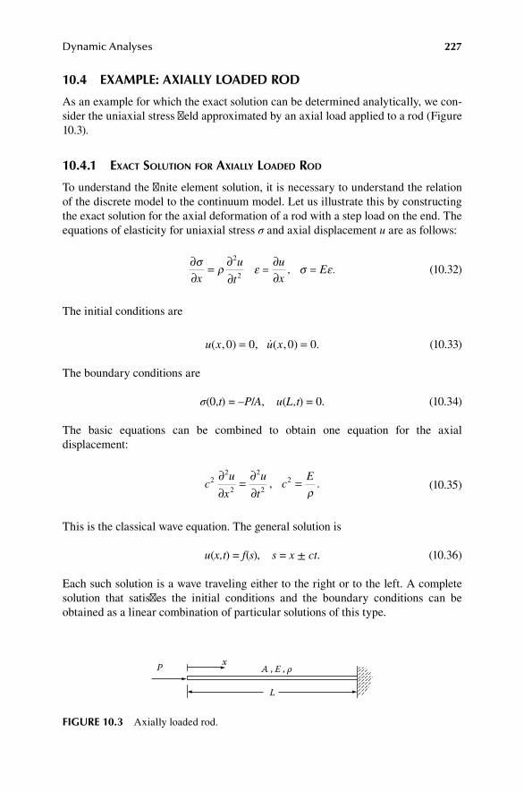
Dynamic Analyses 227
10.4 exaMple: axIally loaded rod
As an example for which the exact solution can be determined analytically, we con-sider the uniaxial stress field approximated by an axial load applied to a rod (Figure 10.3).
10.4.1 exact Solution for axially loaded rod
To understand the finite element solution, it is necessary to understand the relation of the discrete model to the continuum model. Let us illustrate this by constructing the exact solution for the axial deformation of a rod with a step load on the end. The equations of elasticity for uniaxial stress σ and axial displacement u are as follows:
∂∂
= ∂∂
∂∂
= =σ
ρ ε σ εx
u
t
u
xE
2
2, .
(10.32)
The initial conditions are
u x u x( , ) , ( , ) .0 0 0 0= = (10.33)
The boundary conditions are
σ(0,t) = –P/A, u(L,t) = 0. (10.34)
The basic equations can be combined to obtain one equation for the axial displacement:
c
u
x
u
tc
E22
2
2
22∂
∂= ∂
∂=, .
ρ (10.35)
This is the classical wave equation. The general solution is
u(x,t) = f(s), s = x ± ct. (10.36)
Each such solution is a wave traveling either to the right or to the left. A complete solution that satisfies the initial conditions and the boundary conditions can be obtained as a linear combination of particular solutions of this type.
x
L
P A , E , ρ
fIgure 10.3 Axially loaded rod.

228 The Finite Element Method for Mechanics of Solids with ANSYS Applications
For 0 ≤ ct ≤ L, in order to satisfy the initial conditions and the boundary condi-tions, we must take s = x – ct and
u x tP
AEs x ct
x ct
( , ), ,
, .=
− ≤
>
for
for0
(10.37)
σ ( , ), ,
, .x t
P
Ax ct
x ct
=− ≤
>
for
for0
(10.38)
For ct > L, this solution violates the boundary condition at the fixed end. A second solution must be added that counteracts the first one in order to satisfy the boundary condition at x = L. Then, a third solution is added to correct the boundary condition at x = 0, and so forth.
Let us introduce nondimensional variables:
x
x
Lt
ct
Lu
AEu
PL
A
P= = = =, , , .σ
σ
(10.39)
The complete wave solution is shown in Figures 10.4 and 10.5. Figure 10.4 shows the displacement at the loaded end and the displacement of the midpoint versus time. Figure 10.5 shows the stress and displacement versus x at various times.
When a load is suddenly applied to the end of the rod, it causes a stress wave to propagate along the rod. The wave is reflected from the fixed end, doubling the magnitude of the stress. The wave is again reflected when it returns to the loaded end, reducing the stress to the initial value, and so on. There is no displacement of a particle of the rod until the wave reaches it; then the displacement commences and can be calculated from the known uniform strain of the portion of the rod that has
been covered by the wave. The speed of propagation of the wave is c E= /ρ .
.5
1 2 3 4
1.5 3.52.5 4.5
u(0,t )
u(1/2,t )
t = ct/L
t = ct/L
2
1
fIgure 10.4 Exact displacements.

Dynamic Analyses 229
10.4.2 finite eleMent Model
10.4.2.1 one-element ModelFor one-element models with a lumped mass at each end, the finite element equation is
mD t kD t P t( ) ( ) ( )+ = (10.40)
where
m
ALk
AE
L
k
m= = =ρ
ω2
2, , .
(10.41)
For a step load at t = 0,
D t
P
kt( ) ( cos( ))= −1 ω .
(10.42)
ct = L/21 1/2
1ct = L
1
ct = 4L
1ct = 3L/2
21
3/2
2
ct = 2L2 2
1ct = 5L/2
21
3/2
1ct = 3L
1
ct = 7L/21 1/2
uσ
1
0
0
L/2 L L/2 L0
0
x =
t
fIgure 10.5 Exact stress and displacement.
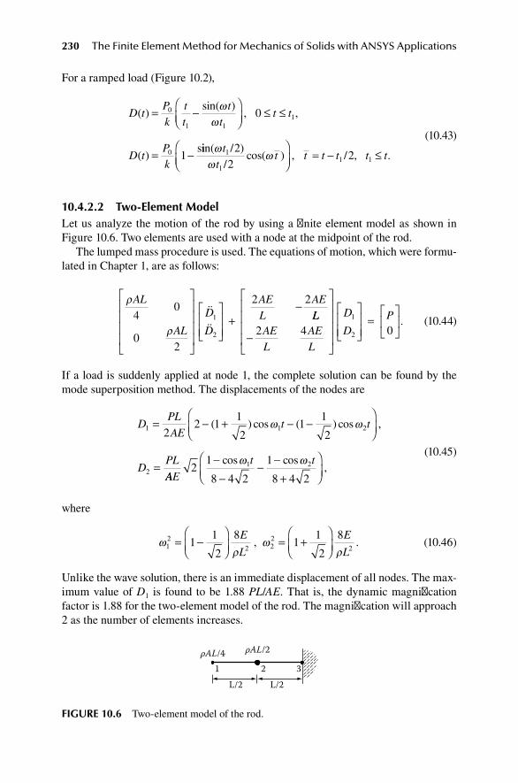
230 The Finite Element Method for Mechanics of Solids with ANSYS Applications
For a ramped load (Figure 10.2),
D tPk
tt
tt
t t
D tPk
( )sin( )
, ,
( )s
= −
≤ ≤
= −
0
1 11
0
0
1
ωω
iin( )cos( ) , / , .
ωω
ωt
tt t t t t t1
11 1
22
2/
/
= − ≤
(10.43)
10.4.2.2 two-element ModelLet us analyze the motion of the rod by using a finite element model as shown in Figure 10.6. Two elements are used with a node at the midpoint of the rod.
The lumped mass procedure is used. The equations of motion, which were formu-lated in Chapter 1, are as follows:
ρ
ρ
AL
AL
D
D
AEL
AE4
0
02
2 2
1
2
+−
LLAEL
AEL
D
DP
−
=
2 4 01
2
.
(10.44)
If a load is suddenly applied at node 1, the complete solution can be found by the mode superposition method. The displacements of the nodes are
DPL
AEt t
DPL
1 1 2
2
22 1
1
21
1
2= − + − −
=
( ) cos ( ) cos ,ω ω
AAE
t t2
1
8 4 2
1
8 4 21 2−
−− −
+
cos cos
,ω ω
(10.45)
where
ωρ
ωρ
12
2 22
21
1
2
81
1
2
8= −
= +
E
L
E
L, .
(10.46)
Unlike the wave solution, there is an immediate displacement of all nodes. The max-imum value of D1 is found to be 1.88 PL/AE. That is, the dynamic magnification factor is 1.88 for the two-element model of the rod. The magnification will approach 2 as the number of elements increases.
ρAL/4 ρAL/2
1 2 3
L/2L/2
fIgure 10.6 Two-element model of the rod.

Dynamic Analyses 231
The solution (10.45) for the two-element model is compared with the exact wave
solution in Figure 10.7 for ρL
E
L
c
2 2
28 81= = . The normalized displacement D(t)/D0,
DPL
AE0 = , is plotted as a function of nondimensional time t ct L= / . The value D(t)/
D0 = 1 is the static solution.
Figure 10.8 is a plot of D2/(PL/AE) versus t showing both the two-element finite element analysis and the wave solution.
0
0.5
1
1.5
2
2.5
0 1 2 3 4 5 6 7 8 9 10ct/L
D1D0
fIgure 10.7 Exact solution for continuum and two-element model.
–0.2
0
0.2
0.4
0.6
0.8
1
1.2
0 1 2 3 4 5 6 7 8 9 10
FEA Wave
D2/D0
ct/L
fIgure 10.8 Displacement of node 2 of two-element model.
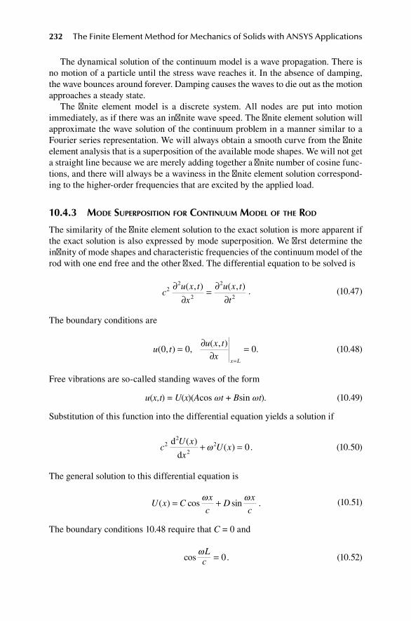
232 The Finite Element Method for Mechanics of Solids with ANSYS Applications
The dynamical solution of the continuum model is a wave propagation. There is no motion of a particle until the stress wave reaches it. In the absence of damping, the wave bounces around forever. Damping causes the waves to die out as the motion approaches a steady state.
The finite element model is a discrete system. All nodes are put into motion immediately, as if there was an infinite wave speed. The finite element solution will approximate the wave solution of the continuum problem in a manner similar to a Fourier series representation. We will always obtain a smooth curve from the finite element analysis that is a superposition of the available mode shapes. We will not get a straight line because we are merely adding together a finite number of cosine func-tions, and there will always be a waviness in the finite element solution correspond-ing to the higher-order frequencies that are excited by the applied load.
10.4.3 Mode SuperpoSition for continuuM Model of the rod
The similarity of the finite element solution to the exact solution is more apparent if the exact solution is also expressed by mode superposition. We first determine the infinity of mode shapes and characteristic frequencies of the continuum model of the rod with one end free and the other fixed. The differential equation to be solved is
c
u x t
x
u x t
t2
2
2
2
2
∂∂
= ∂∂
( , ) ( , ) .
(10.47)
The boundary conditions are
u tu x t
xx L
( , ) ,( , )
.0 0 0= ∂∂
==
(10.48)
Free vibrations are so-called standing waves of the form
u(x,t) = U(x)(Acos ωt + Bsin ωt). (10.49)
Substitution of this function into the differential equation yields a solution if
c
U x
xU x2
2
22 0
d
d
( )( )+ =ω .
(10.50)
The general solution to this differential equation is
U x C
x
cD
x
c( ) cos sin= +ω ω
.
(10.51)
The boundary conditions 10.48 require that C = 0 and
cosω Lc = 0 . (10.52)

Dynamic Analyses 233
This yields the characteristic frequencies:
ω
π= n c
Ln
2, .odd
(10.53)
The family of mode shapes is therefore
U x
xcnn( ) sin= ω
.
(10.54)
This exact solution for the natural frequencies 10.53 is compared to the approxi-mate solution obtained by the finite element analysis using the lumped mass and consistent mass in Table 10.1. Convergence toward the first frequency is shown in
taBle 10.1 finite element analysis
number of elements
exact2πω1L/c
fealumped Mass
feaconsistent Mass
1 0.25 0.22508 0.27566
2 0.25 0.243624 0.256465
0.75 0.588160 0.895931
3 0.25 0.247154 0.252865
0.75 0.675237 0.826993
1.25 0.922391 1.50029
4 0.25 0.248397 0.251609
0.75 0.707374 0.793737
1.25 1.05886 1.44185
1.75 1.24877 2.0804
5 0.25 0.248973 0.251029
0.75 0.722548 0.777971
1.25 1.12540 1.37832
1.75 1.41808 2.06686
2.25 1.57195 2.65843
10 0.25 0.249753 0.250257
0.75 0.743080 0.756957
1.25 1.21812 1.28232
1.75 1.66316 1.83891
2.25 2.06726 2.43830
100 0.25 0.249997 0.250003
0.75 0.749931 0.750069
1.25 1.24968 1.25032
1.75 1.74912 1.75088
2.25 2.24813 2.25187
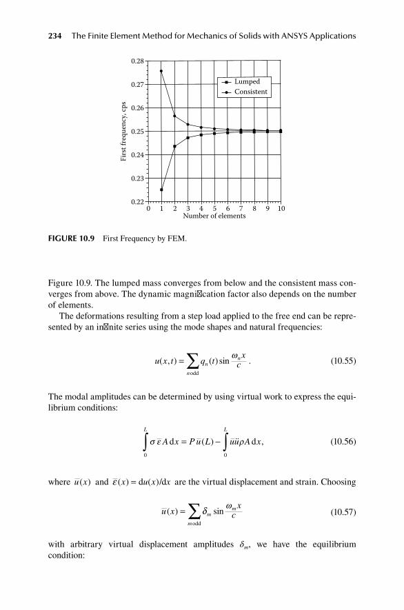
234 The Finite Element Method for Mechanics of Solids with ANSYS Applications
Figure 10.9. The lumped mass converges from below and the consistent mass con-verges from above. The dynamic magnification factor also depends on the number of elements.
The deformations resulting from a step load applied to the free end can be repre-sented by an infinite series using the mode shapes and natural frequencies:
u x t q tx
cnn
n
( , ) ( ) sin= ∑ ω
odd
.
(10.55)
The modal amplitudes can be determined by using virtual work to express the equi-librium conditions:
σ ε ρA x P u L uu A x
L L
d d0 0∫ ∫= −( ) ,
(10.56)
where u x( ) and ε ( ) ( )x u x x= d /d are the virtual displacement and strain. Choosing
u xx
cmm
m
( ) sin= ∑ δ ω
odd
(10.57)
with arbitrary virtual displacement amplitudes δm, we have the equilibrium condition:
0.22
0.23
0.24
0.25
0.26
0.27
0.28
0 1 2 3 4 5 6 7 8 9 10
Firs
t fre
quen
cy, c
ps
Number of elements
LumpedConsistent
fIgure 10.9 First Frequency by FEM.

Dynamic Analyses 235
AE qnm
L
n xL
m xL
x
Pm
n m
L
mn
m
δπ π π
δπ
0
2
24 2 2∫∑∑
=
cos cos d
sin22 2 2
0m
n m
L
mn
A qn x
Lm x
Lx∑ ∫∑∑− ρ δ
π πsin .sin d
(10.58)
The sums are on odd integers. Since
sin2
sin2
d for , sinn x
Lm x
Lx n m
n xL
π π π= ≠∫ 02
0LL
xL
n m
n xL
m xL
x
L
L
= =∫
∫
2
0
0
2
2 2
d for
cos cos d
,
π π == ≠
=∫02 2
2
0
for , d forn mn x
Lx
Ln
L
cosπ == m,
(10.59)
we find
δρ π π
m m m
m
ALq
AEm
Lq P
m
2 8 20
2 2
+ −
=∑ sin .
(10.60)
This relation must hold identically for all δm. Therefore,
q
m c
Lq
P
AL
mm m+ =
2 2 2
24
22
π πρ
sin . (10.61)
The solution for zero initial conditions is
q t
PL
AE
m
mtm m( )
( )( )= −8 21
2 2
sin /cos
ππ
ω .
(10.62)
The displacement of the free end (x = L) is
u L tPL
AE mtm
m
( , ) ( )= −∑ 81
2 2πωcos
odd
.
(10.63)
The maximum occurs when t = 2L/c or ωmt = mπ:

236 The Finite Element Method for Mechanics of Solids with ANSYS Applications
max ( , )u L tPL
AE mn
= ∑16 12 2π
odd
.
(10.64)
Since
182
2
mn odd
∑ = π
(10.65)
we find
max ( , )u L tPL
AE= 2 . (10.66)
That is, the dynamic displacement due to the step load is twice the static value, a dynamic magnification factor of 2. However, the series 10.65 converges slowly, so the magnification factor computed using any partial number of modes is much less than 2 as shown in Table 10.2.
We are able to find the exact solution to the continuum model of the rod (1D), but it is generally not possible to do so for 2D or 3D continuum models. The wave pattern is so complex that only numerical methods are feasible. In this case, the finite element model can provide a satisfactory approximation if properly interpreted.
10.5 exaMple: Short BeaM
In Section 5.6.4, the short cantilever beam was analyzed as a plane stress problem using rectangular elements. The same layout (see Figure 10.10) will now be used for the determination of the lower frequencies and mode shapes.
For N unsupported nodes, there are 2N equations and therefore 2N natural fre-quencies. These frequencies approximate the lower natural frequencies of the body, which has of course infinitely many natural frequencies. Table 10.3 shows the results using the consistent mass matrix and the results using the lumped mass matrix together with the four-node rectangle (Section 15.17). The values are for ν is 1/3. The exact solution is unknown for this example.
taBle 10.2 Magnification factor
number of Modes 1 2 3 4
Magnification factor 1.621 1.801 1.866 1.899

Dynamic Analyses 237
10.6 dynaMIc analySIS WIth daMpIng
Damping was not included in the preceding analysis, but motions of real bodies are always damped. This damping is of little importance over a short time scale, but is essential for the analysis of the steady-state response. Damping arises from many dissipative processes accompanying the motion, the details of which are often not known. Damping is generally modeled by including a damping force proportional to velocities. The general equation 10.14 then becomes
MD VD KD F + + = . (10.67)
The damping matrix V is not generally determined by merging element matrices because the details of the damping mechanisms are not known. A typical assumption is*
V M K K= + + ∑α β βi i
i
(10.68)
* The symbol α also occurs in the following formulation of numerical integration. To make it clear which alpha is meant, we may write alphad and betad for the damping coefficients.
taBle 10.3 Short Beam
number of elements
lumped Mass lumped Mass consistent Mass consistent Mass
ωω ρρ12a E/ ωω ρρ2
2a E/ ωω ρρ12a E/ ωω ρρ2
2a E/
1 0.59043 1.35962 0.77648 1.74559
16 0.66181 1.57645 0.67676 1.60033
100 0.65754 1.58141 0.65992 1.58531
256 0.65634 1.58154 0.65728 1.58311
10,000 0.65515 1.58123 0.65515 1.58129
1
1
fIgure 10.10 Lumped mass model.

238 The Finite Element Method for Mechanics of Solids with ANSYS Applications
where Ki is the part of the stiffness matrix due to material i. This is called Rayleigh damping or proportional damping. The coefficients are determined directly by experiments that measure the decay in amplitude of free vibrations. Proportional damping has some basis in theory, which we will now demonstrate.
10.6.1 ViScoelaStic daMping
One damping mechanism is the internal dissipation of the material due to inelastic behavior. If the viscous loss is small and as there are no jumps in strain when inertia is included, the material may be adequately modeled by a two element Kelvin–Voigt model for both shearing and volume change:
s e e= +2 2µ η, (10.69)
13
τ κε ζεkk kk kk= + . (10.70)
Since skm = τkm – τiiδkm and ekm = εkm – εiiδkm, Equations 10.69 and 10.70 are equivalent to the single constitutive equation
τ µε λε δ ηε λ ε δkm km ii km km ii km= + + +2 2 D , (10.71)
where
λ κ µ λ ζ η= − = −2
323
, .D
(10.72)
There are four independent material constants: two elasticities and two viscosities. In matrix form, 10.71 is
ττ εε εε= +C CD , (10.73)
where C and CD have the same form as in the elasticity problem if we define artificial Poisson ratios:
νλ
λ µν
λλ η
=+
=+2 2 2 2
, .DD
D
(10.74)
The global equations of dynamical equilibrium are
A F MDT dττVn
Vn
∫∑ = − ,
(10.75)
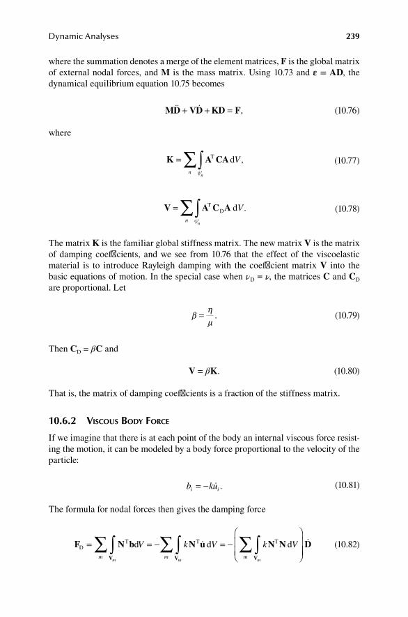
Dynamic Analyses 239
where the summation denotes a merge of the element matrices, F is the global matrix of external nodal forces, and M is the mass matrix. Using 10.73 and ε = AD, the dynamical equilibrium equation 10.75 becomes
MD VD KD F + + = , (10.76)
where
K A CA= ∫∑ T dV
nn V
,
(10.77)
V A C A= ∫∑ TD d
Vn
Vn
.
(10.78)
The matrix K is the familiar global stiffness matrix. The new matrix V is the matrix of damping coefficients, and we see from 10.76 that the effect of the viscoelastic material is to introduce Rayleigh damping with the coefficient matrix V into the basic equations of motion. In the special case when νD = ν, the matrices C and CD are proportional. Let
β
ηµ
= .
(10.79)
Then CD = βC and
V = βK. (10.80)
That is, the matrix of damping coefficients is a fraction of the stiffness matrix.
10.6.2 ViScouS Body force
If we imagine that there is at each point of the body an internal viscous force resist-ing the motion, it can be modeled by a body force proportional to the velocity of the particle:
b kui i= − . (10.81)
The formula for nodal forces then gives the damping force
F N b N u N NV V V
DT T Td d d= = − = −
∫∑ ∫∑ ∫∑V k V k V
m m mm m m
D
(10.82)
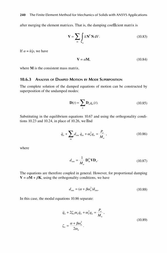
240 The Finite Element Method for Mechanics of Solids with ANSYS Applications
after merging the element matrices. That is, the damping coefficient matrix is
V N NV
= ∫∑ k V
mm
T d .
(10.83)
If α = k/ρ, we have
V = αM, (10.84)
where M is the consistent mass matrix.
10.6.3 analySiS of daMped Motion By Mode SuperpoSition
The complete solution of the damped equations of motion can be constructed by superposition of the undamped modes:
D D( ) ( )t q tn
n
n= ∑ .
(10.85)
Substituting in the equilibrium equations 10.67 and using the orthogonality condi-tions 10.23 and 10.24, in place of 10.26, we find
q d q qP
Mn nm m
m
n nn
n
+ + =∑ ω 2 ,
(10.86)
where
d
Mnmn
m n= 1D VDT .
(10.87)
The equations are therefore coupled in general. However, for proportional damping V = αM + βK, using the orthogonality conditions, we have
dnm n nm= +( )α βω δ2 . (10.88)
In this case, the modal equations 10.86 separate:
q q qP
Mn n n n n nn
n
nn
n
+ + =
= +
2
2
2
2
ζ ω ω
ζα βω
ω
,
.
(10.89)
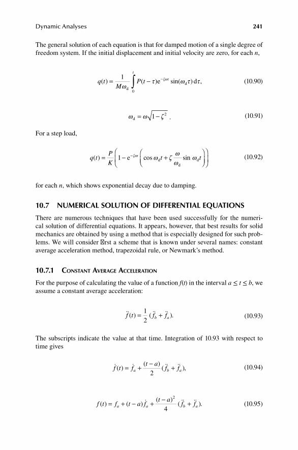
Dynamic Analyses 241
The general solution of each equation is that for damped motion of a single degree of freedom system. If the initial displacement and initial velocity are zero, for each n,
q tM
P t
t
( ) ( ) sin( )= − −∫1
0ω
τ ω τ τζωτ
dde d ,
(10.90)
ω ω ζd = −1 2 . (10.91)
For a step load,
q tP
Kt tt( ) = − +
−1 e cos sind
dd
ζω ω ζω
ωω
(10.92)
for each n, which shows exponential decay due to damping.
10.7 nuMerIcal SolutIon of dIfferentIal equatIonS
There are numerous techniques that have been used successfully for the numeri-cal solution of differential equations. It appears, however, that best results for solid mechanics are obtained by using a method that is especially designed for such prob-lems. We will consider first a scheme that is known under several names: constant average acceleration method, trapezoidal rule, or Newmark’s method.
10.7.1 conStant aVerage acceleration
For the purpose of calculating the value of a function f(t) in the interval a ≤ t ≤ b, we assume a constant average acceleration:
f t f fb a( ) ( ).= +1
2 (10.93)
The subscripts indicate the value at that time. Integration of 10.93 with respect to time gives
f t f
t af fa b a( )
( )( ),= + − +
2 (10.94)
f t f t a ft a
f fa a b a( ) ( )( )
( ).= + − + − +
2
4 (10.95)
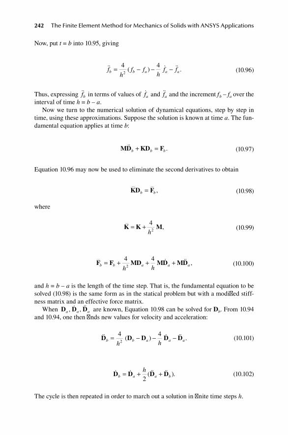
242 The Finite Element Method for Mechanics of Solids with ANSYS Applications
Now, put t = b into 10.95, giving
f
hf f
hf fb b a a a= − − −4 4
2( ) .
(10.96)
Thus, expressing fb in terms of values of fa and fa and the increment fb – fa over the interval of time h = b – a.
Now we turn to the numerical solution of dynamical equations, step by step in time, using these approximations. Suppose the solution is known at time a. The fun-damental equation applies at time b:
MD KD F
b b b+ = . (10.97)
Equation 10.96 may now be used to eliminate the second derivatives to obtain
KD Fb b= , (10.98)
where
K K M= + 4
2h,
(10.99)
F F MD MD MDb b a a a
h h= + + +4 4
2 ,
(10.100)
and h = b – a is the length of the time step. That is, the fundamental equation to be solved (10.98) is the same form as in the statical problem but with a modified stiff-ness matrix and an effective force matrix.
When D D Da a a, , are known, Equation 10.98 can be solved for Db. From 10.94 and 10.94, one then finds new values for velocity and acceleration:
D D D D Db b a a a
h h= − − −4 4
2( ) .
(10.101)
D D D Db a a b
h= + +2( ).
(10.102)
The cycle is then repeated in order to march out a solution in finite time steps h.

Dynamic Analyses 243
10.7.2 general newMark Method
Instead of using the average acceleration, the method can be improved by taking some value that better approximates the first integration over the interval. Let us consider first, in place of 10.94 and 10.95, the mathematical identities:
f f f t tb a
a
b
= + ∫ ( ) d ,
(10.103)
f f hf b t f t tb a a
a
b
= + + −∫ ( ) ( ) d .
(10.104)
Instead of constant acceleration, we can use the approximate integration formula
f t t W f W fa
b
a b( ) d∫ = +1 2 .
(10.105)
The weighting numbers Wi are determined by requiring that the integration formula yield the exact result in case f is constant; this gives W1 + W2 = h, or in the usual notation
W2 = δh, W1 = (1 – δ)h. (10.106)
In the same way, we find
( ) ( )b t f t t h f h fa
b
a b− = −
+∫
d12
2 2α α .
(10.107)
Therefore, 10.103 and 10.104 give the fundamental approximations
f hf f hfb b a a= + + −δ ( )1 δ , (10.108)
f h f f hf h fb b a a a= + + + −
α α2 212
,
(10.109)

244 The Finite Element Method for Mechanics of Solids with ANSYS Applications
in place of 10.96. The constant average acceleration formulas are the special case when δ = 1/2 and α = 1/4.*
10.7.3 general MethodS
The Newmark scheme is only one way of marching the solution forward in time. A great many other systems have been worked out and analyzed. A general form of the relations is as follows:
f h f L f f f
f hf L f
b b a a a
b b a
= +
= +
α
δ
20
1
( , ),
( ,
,
ffa ),
(10.110)
where L0 and L1 are linear combinations of the indicated arguments and possibly of the values at other prior times, and α and δ are constants.
10.7.3.1 Implicit Methods in general If α and δ are not zero, the system is called implicit because the value at time b is not explicitly determined by the state at time a. In this case, we can solve 10.110 for fb as was carried out above. Substitution of the result into 10.97 again yields 10.98 with
K K M
F F M D D D
= +
= +
1
1
2
2 0
α
α
h
hLb b a a a
,
( , , ).
(10.111)
Solution of 10.98 gives fb, and then 10.110 determines fb and fb .
10.7.3.2 explicit Methods in general If α and δ are zero, the scheme 10.110 is called explicit because the value of the func-tion at time b is explicitly determined by the state at time a. In this case, we substitute 10.110 into 10.97 to obtain a formula for the second derivatives:
D M F K D D Db b a a aL= −−10[ ( , , )]. (10.112)
Equations 10.110 with α = 0 determine Db and Db.
D L D D
D L D D D
b a a
b a a a
=
=
1
0
( , ),
( , , ).
(10.113)
* ANSYS input δ γ α λ= + = +1
2
1
41 2, ( ) , default γ = 0.005.

Dynamic Analyses 245
Note that the stiffness matrix does not have to be inverted in the explicit method. Instead, the mass matrix is inverted. This is a trivial matter when M is diagonal as in the lumped mass model. We will not develop the solution by explicit methods in this book.
10.7.4 StaBility analySiS of newMark’S Method
Let us consider the free vibration of the 1 degree of freedom system:
f f+ =ω 2 0.
(10.114)
The exact solution is f(t) = Ceiωt. At time b, fb = Ceiωb. At time a, fa = Ceiωa. Thus, fb = eiωhfa, h = b – a. We seek a numerical solution of the same character but with pos-sibly varying amplitude and somewhat different frequency: f t c t i t( ) ( )= e ω . For this
numerical solution, fcc fb
b
a
i ha= e ω . That is,
fb = λfa (10.115)
where λ is a complex number. At time b, from 10.114, f fb b+ =ω 2 0. Using 10.109, we find
f f hf h f h fb a a a b− − − −
+ =
12
02 2 2α α ω .
(10.116)
Using 10.114 for t = a to eliminate fa , we have
( )1 112
2 2 2+ = − −
+βαω α ωf h f hfb a a .
(10.117)
Using 10.114 to eliminate the second derivatives in 10.108, we have
δ ω δ ωh f f h f fb b a a2 21+ = − − + ( ) . (10.118)
Equations 10.117 and 10.118 have the form
Aua = Bub, (10.119)
where
u =
f
f,
A =− −
− −
112
1 1
2 2
2
α ω
δ ω
h h
h( )
,
B = +
( )1 0
1
2 2
2
α ω
δ ω
h
h.
(10.120)
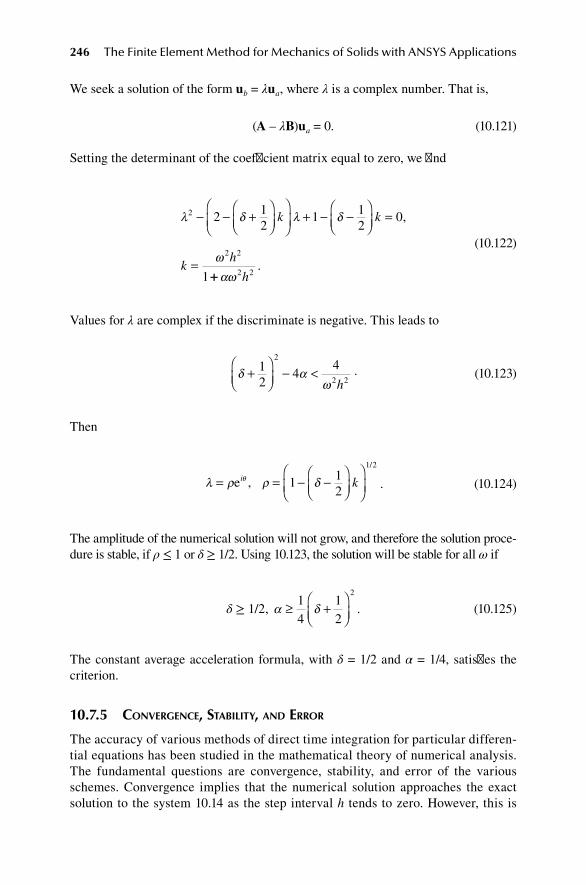
246 The Finite Element Method for Mechanics of Solids with ANSYS Applications
We seek a solution of the form ub = λua, where λ is a complex number. That is,
(A – λB)ua = 0. (10.121)
Setting the determinant of the coefficient matrix equal to zero, we find
λ δ λ δ
ω
2
2 2
2 12
1 12
0
1
− − +
+ − −
=
=
k k
kh
,
++ αω 2 2h.
(10.122)
Values for λ are complex if the discriminate is negative. This leads to
δ α
ω+
− <12
44
2
2 2h.
(10.123)
Then
λ ρ ρ δθ= = − −
ei k,
/
1 12
1 2
.
(10.124)
The amplitude of the numerical solution will not grow, and therefore the solution proce-dure is stable, if ρ ≤ 1 or δ ≥ 1/2. Using 10.123, the solution will be stable for all ω if
δ ≥ 1/2, α δ≥ +
14
12
2
. (10.125)
The constant average acceleration formula, with δ = 1/2 and α = 1/4, satisfies the criterion.
10.7.5 conVergence, StaBility, and error
The accuracy of various methods of direct time integration for particular differen-tial equations has been studied in the mathematical theory of numerical analysis. The fundamental questions are convergence, stability, and error of the various schemes. Convergence implies that the numerical solution approaches the exact solution to the system 10.14 as the step interval h tends to zero. However, this is
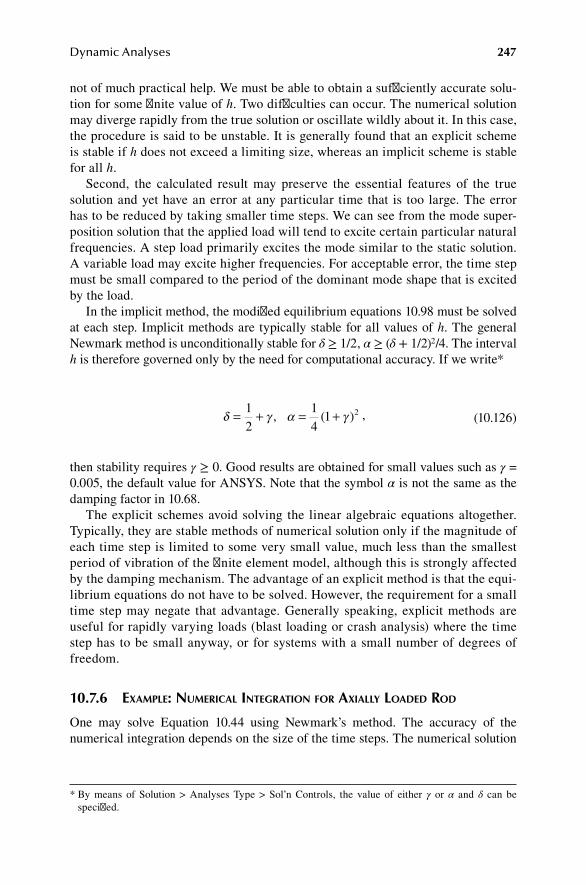
Dynamic Analyses 247
not of much practical help. We must be able to obtain a sufficiently accurate solu-tion for some finite value of h. Two difficulties can occur. The numerical solution may diverge rapidly from the true solution or oscillate wildly about it. In this case, the procedure is said to be unstable. It is generally found that an explicit scheme is stable if h does not exceed a limiting size, whereas an implicit scheme is stable for all h.
Second, the calculated result may preserve the essential features of the true solution and yet have an error at any particular time that is too large. The error has to be reduced by taking smaller time steps. We can see from the mode super-position solution that the applied load will tend to excite certain particular natural frequencies. A step load primarily excites the mode similar to the static solution. A variable load may excite higher frequencies. For acceptable error, the time step must be small compared to the period of the dominant mode shape that is excited by the load.
In the implicit method, the modified equilibrium equations 10.98 must be solved at each step. Implicit methods are typically stable for all values of h. The general Newmark method is unconditionally stable for δ ≥ 1/2, α ≥ (δ + 1/2)2/4. The interval h is therefore governed only by the need for computational accuracy. If we write*
δ γ α γ= + = +1
214
1 2, ( ) ,
(10.126)
then stability requires γ ≥ 0. Good results are obtained for small values such as γ = 0.005, the default value for ANSYS. Note that the symbol α is not the same as the damping factor in 10.68.
The explicit schemes avoid solving the linear algebraic equations altogether. Typically, they are stable methods of numerical solution only if the magnitude of each time step is limited to some very small value, much less than the smallest period of vibration of the finite element model, although this is strongly affected by the damping mechanism. The advantage of an explicit method is that the equi-librium equations do not have to be solved. However, the requirement for a small time step may negate that advantage. Generally speaking, explicit methods are useful for rapidly varying loads (blast loading or crash analysis) where the time step has to be small anyway, or for systems with a small number of degrees of freedom.
10.7.6 exaMple: nuMerical integration for axially loaded rod
One may solve Equation 10.44 using Newmark’s method. The accuracy of the numerical integration depends on the size of the time steps. The numerical solution
* By means of Solution > Analyses Type > Sol’n Controls, the value of either γ or α and δ can be specified.
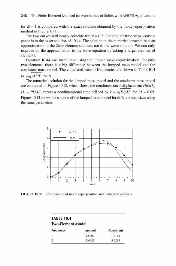
248 The Finite Element Method for Mechanics of Solids with ANSYS Applications
for dt = 1 is compared with the exact solution obtained by the mode superposition method in Figure 10.11.
The two curves will nearly coincide for dt = 0.2. For smaller time steps, conver-gence is to the exact solution of 10.44. The solution in the numerical procedure is an approximation to the finite element solution, not to the wave solution. We can only improve on the approximation to the wave equation by taking a larger number of elements.
Equation 10.44 was formulated using the lumped mass approximation. For only two elements, there is a big difference between the lumped mass model and the consistent mass model. The calculated natural frequencies are shown in Table 10.4
as ω ρL E2 / rad/s.The numerical solution for the lumped mass model and the consistent mass model
are compared in Figure 10.12, which shows the nondimensional displacement D(t)/D0,
D0 = PL/AE, versus a nondimensional time defined by t t E L= /ρ 2 for ∆t = 0 05. .
Figure 10.13 shows the solution of the lumped mass model for different step sizes using the same parameters.
taBle 10.4 two-element Model
frequency lumped consistent
1 1.5307 1.6114
2 3.6955 5.6293
0
1
2
3
4
5
0 1 2 3 4 5 6 7 8 9 10
Disp
lace
men
t
Time
dt = 1
exact
fIgure 10.11 Comparison of mode superposition and numerical analysis.

Dynamic Analyses 249
10.8 exaMple: analySIS of Short BeaM
Let us again consider the plane stress problem shown in Figure 10.14 and use the rectangular elements with lumped mass (Figure 10.10). We will use nondimensional values a = 1, b = 1, p = 1, ρ = 1, E = 1, ν = 1/3. The element layout used was a 10 × 10 grid of 100 elements. The body is initially at rest and a step load p is applied. The calculated displacement of the corner without damping, using a time step h = 0.1, is plotted in Figure 10.15.
0
0.2
0.4
0.6
0.8
1
1.2
1.4
1.6
1.8
2
0 1 2 3 4 5 6 7 8 9 10
Consistent Lumped
Time
Disp
lace
men
t
fIgure 10.12 Lumped mass and consistent mass.
dt = 0.5 dt = 0.1
0 1 2 3 4 5 6 7 8 9 10Time
0
0.2
0.4
0.6
0.8
1
1.2
1.4
1.6
1.8
2
Disp
lace
men
t
fIgure 10.13 Lumped mass model.
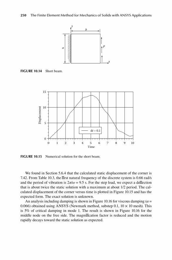
250 The Finite Element Method for Mechanics of Solids with ANSYS Applications
We found in Section 5.6.4 that the calculated static displacement of the corner is 7.42. From Table 10.3, the first natural frequency of the discrete system is 0.66 rad/s and the period of vibration is 2π/ω = 9.5 s. For the step load, we expect a deflection that is about twice the static solution with a maximum at about 1/2 period. The cal-culated displacement of the corner versus time is plotted in Figure 10.15 and has the expected form. The exact solution is unknown.
An analysis including damping is shown in Figure 10.16 for viscous damping (α = 0.066) obtained using ANSYS (Newmark method, substep 0.1, 10 × 10 mesh). This is 5% of critical damping in mode 1. The result is shown in Figure 10.16 for the middle node on the free side. The magnification factor is reduced and the motion rapidly decays toward the static solution as expected.
yb
p
x
a
fIgure 10.14 Short beam.
0
5
10
15
0 1 2 3 4 5 6 7 8 9 10
Disp
lace
men
t
Time
dt = 0.1
fIgure 10.15 Numerical solution for the short beam.

Dynamic Analyses 251
10.9 proBleMS
1. Determine the mode shapes and frequencies for the rod shown in Figure 10.17 using two elements by solving the differential equation. Normalize the mode shapes so that Mn = 1.
2. Determine the mode shapes and frequencies for the rod shown in Figure 10.17 for two elements by using ANSYS and compare with the solution of problem 1. See Section 15.16. Note that ANSYS reports the frequencies in cps.
3. Consider a rod that is loaded at the end x = 0 and fixed at the end x = L (see Figure 10.17). Divide the rod into two finite elements by a node at the center and use the lumped mass approach. For A = 1, E = 1, ρ = 1.(a) Solve by hand for the mode shapes and frequencies. Normalize the
mode shapes so that the generalized mass is 1 for each mode.(b) Solve using ANSYS and compare results. See Section 15.16. Note that
ANSYS reports frequencies in cps.
0
2
4
6
8
10
12
14
0 5 10 15 20 25 30 35 40 45 50
Disp
lace
men
t
Time
fIgure 10.16 Damped motion.
x
L
P A , E , ρ
fIgure 10.17 Axially loaded rod.

252 The Finite Element Method for Mechanics of Solids with ANSYS Applications
4. Consider a rod that is loaded at the end x = 0 and fixed at the end x = L (see Figure 10.17). Divide the rod into two finite elements by a node at the center and use the lumped mass approach to derive the equations of motion.(a) Calculate the two natural frequencies of vibration.(b) Determine the nodal displacements for the case of a constant load sud-
denly applied to the end x = 0 at time t = 0.(c) Compare the finite element solution for the displacement at node 1
with the wave propagation analysis by plotting the displacement versus time.
5. Given the axially loaded rod shown in Figure 10.17 with A = 1, L = 1, E = 100, ρ = 2. The load is ramped up as shown in Figure 10.2 with P0 = 3 and t1 = 1. Use ANSYS to determine the displacement of the end for 0 ≤ t ≤ 2. Use one element with lumped mass and numerical integration. Compare the maximum displacement with the exact solution (10.3.8)–(10.3.9).
6. Use ANSYS to determine the first two mode shapes and natural frequen-cies for the plane stress problem shown in Figure 10.18 for a = b = 1, E = 1, ν = 1/3, ρ = 1. Use the four-node Plane 182 element and a 10 × 10 mesh. Determine the lowest two frequencies and view the mode shapes. See Section 15.17. (A printable list can be obtained via Utility Menu > List > Results > Load Step Summary.) Record the x component of displacements of nodes on the loaded edge for each mode for use in problem 7.
a
yb
p
x
fIgure 10.18 Plane stress extension.
yb
p
x
a
fIgure 10.19 Plane stress bending.

Dynamic Analyses 253
7. Use the results of problem 6 to calculate the x displacement of the corner for step load p = 10 uniformly distributed over the edge x = 1 using only the first two modes.
8. Given the plane stress problem shown in Figure 10.19 with a = b = 1, E = 1, ν = 1/3, ρ = 1, p = 1. Solve by ANSYS for a step load by the Newmark method 0 < t ≤ 50 using dt = 0.1 including damping with α = 0.066. Use the four-node element without extra degree of freedom, and a 10 × 10 mesh. See Section 15.8. Submit a graph of UY at the center of the loaded side versus time (after adjusting colors to obtain black lines on a white background).
9. The finite element equations for dynamics with damping are MD VD KD F + + = . Determine the modified stiffness matrix K and the modified force matrix F when the Newmark method is used to solve these equations.
BIBlIography
Baruh, H., Analytical Dynamics. WCB/McGraw-Hill, New York, 1999.Benaroya, H., and M. L. Nagurka, Mechanical Vibration, 3rd ed., CRC Press, Boca Raton,
FL, 2010.Bottega, W. J., Engineering Vibrations, CRC Press, Boca Raton, FL, 2006.

255
11 Linear Elastic Fracture Mechanics
11.1 fracture crIterIon
If a crack has developed in a structure, the crack may propagate catastrophically when the stress intensity and the crack length combine to reach a critical situation. The basic formulation of the continuum theory of initiation of crack propagation will now be reviewed.*
Let us first consider an elastic sheet of thickness t with a plane crack of length L = 2a through the sheet (Figure 11.1). The sheet is loaded in uniaxial tension S. After applying the load, there is a strain energy U stored in the body that depends on the magnitude of the load, the material properties, and the geometry of the body. In particular, U depends on the crack length L. If, at some load, the crack extends by amount dL, there is a release of the stored strain energy:
d dU = ∂
∂UL
L. (11.1)
At the same time, energy of amount dE is expended to fracture the material and cre-ate a new free surface dA = 2tdL:
dE = GdA, (11.2)
where G is the energy of crack growth per unit area. The fundamental assumption is that G is a material constant that has to be determined by materials testing. This is known as the Griffith hypothesis.
The energy balance for the crack extension requires that strain energy release rate must provide the energy needed for crack growth. Therefore, crack initiation can only occur if
∂∂U
GL
t= 2 . (11.3)
The theory can be put in a more compact form if we define a so-called stress inten-sity factor K by
K
E
t L= ∂
∂U
(11.4)
* For a more complete treatment, see Dill: Chapter 6. Refer to Preface.

256 The Finite Element Method for Mechanics of Solids with ANSYS Applications
and let
K Ec = 2 G .
(11.5)
Then the condition for crack propagation becomes
K = Kc. (11.6)
The critical stress intensity factor Kc is a material property to be determined by materials testing.
To determine K, we must perform a stress analysis of the body. The situation near the crack tip is certainly not modeled accurately by linear elasticity. The continuum model itself is probably not sufficient to describe the material behavior near the crack tip. However, a reasonably accurate prediction of strain energy release rate that is useful in engineering fracture mechanics results from this model.
Once the elasticity problem has been solved, the stored energy can be calculated. The strain energy per unit volume U of the material is such that
τε
µε λ ε ε ε δijij
ij ij
U= = + + +∂∂
2 11 22 33( ) .
(11.7)
Therefore,
U km km kk mm
mk
km km
mk
= +( ) = ( )∑∑ ∑∑12
212
µε ε λε ε τ ε .
(11.8)
The total stored energy is
U = ∫∫∫ U Vd .
(11.9)
Integrating by parts and using the divergence theorem, neglecting the body force and the inertial force, we find that
U = ⋅∫∫1
2T u dA.
(11.10)
This equation will be used to calculate the stored energy.
S 2l
xy
2a 2b
S
fIgure 11.1 Cracked sheet in tension.

Linear Elastic Fracture Mechanics 257
11.1.1 analySiS of Sheet
The sheet is loaded in uniform tension in the y direction. The body is approximately in a state of plane stress (τk3 = 0). The complete solution is conveniently divided into two parts: the solution with no crack and the solution that removes the stress along the crack face. The solution for no crack is uniaxial tension:
τxx = 0, τyy = S, τxy = 0. (11.11)
This solution leaves a tensile stress τyy = S on each crack face. We therefore need to construct a solution for τyy = –S on each crack face (and no other loads) so that the combined solution will have zero tractions on the crack face. This second solution is known as the crack opening problem.
The exact solution of the crack opening problem for a body of finite extent is unknown, but if the crack is small, the solution for a body of infinite extend is a good approximation. This solution is known. The displacement of the crack surface is*
u
S
Ea xy = −2 2 2 .
(11.12)
The stress vector on the upper crack face is T = Sj. The stored energy is therefore
U = −
=∫412
24
0
2 22 2
SS
Ea x t x
L S t
E
a
dπ
, (11.13)
where the crack length L = 2a. The total stored energy of the sheet is therefore
U U= +0
π L S t
E
2 2
4 (11.14)
where the first term is the energy for zero crack length. From this expression, we find
K S a= π . (11.15)
The solution for a body of finite dimensions has the form
K S a= α π , (11.16)
where α > 1 is a numerical factor that depends on the actual dimensions. The finite element method will be used to determine the factor α.
Crack growth initiates when S and crack length L reach critical levels such that
K = Kc. (11.17)
* Dill, p. 243. Refer to Preface.
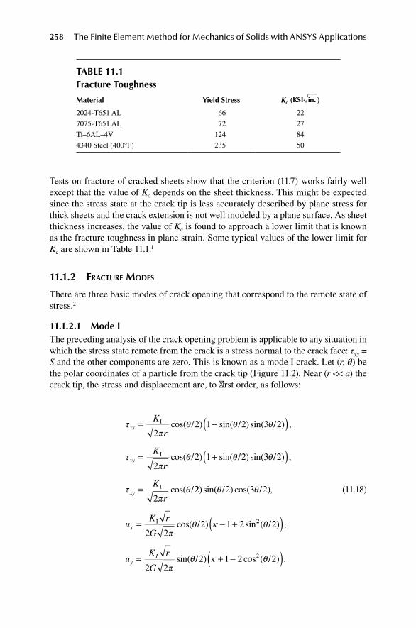
258 The Finite Element Method for Mechanics of Solids with ANSYS Applications
Tests on fracture of cracked sheets show that the criterion (11.7) works fairly well except that the value of Kc depends on the sheet thickness. This might be expected since the stress state at the crack tip is less accurately described by plane stress for thick sheets and the crack extension is not well modeled by a plane surface. As sheet thickness increases, the value of Kc is found to approach a lower limit that is known as the fracture toughness in plane strain. Some typical values of the lower limit for Kc are shown in Table 11.1.1
11.1.2 fracture ModeS
There are three basic modes of crack opening that correspond to the remote state of stress.2
11.1.2.1 Mode IThe preceding analysis of the crack opening problem is applicable to any situation in which the stress state remote from the crack is a stress normal to the crack face: τyy = S and the other components are zero. This is known as a mode I crack. Let (r, θ) be the polar coordinates of a particle from the crack tip (Figure 11.2). Near (r << a) the crack tip, the stress and displacement are, to first order, as follows:
τπ
θ θ θ
τπ
xx
yy
K
r
K
= −( )
=
I
I
/ / /2
2 1 2 3 2
2
cos( ) sin( ) sin( ) ,
rr
K
rxy
cos( ) sin( ) sin( ) ,
cos(
θ θ θ
τπ
θ
/ / /
/I
2 1 2 3 2
2
+( )
= 22 2 3 2
2 22 1 2
)sin( ) cos( ),
cos( ) sin
θ θ
πθ κ
/ /
/IuK r
Gx = − + 22
2
2
2 22 1 2 2
( ) ,
sin( ) cos ( ) .
θ
πθ κ θ
/
/ /
( )
= + −( )uK r
Gy
I
(11.18)
taBle 11.1 fracture toughness
Material yield Stress Kc (KSI in. )
2024-T651 AL 66 22
7075-T651 AL 72 27
Ti–6AL–4V 124 84
4340 Steel (400°F) 235 50

Linear Elastic Fracture Mechanics 259
where K r yy rI lim= = →( | )2 0 0π τ θ and κ = (3 – ν)/(1 + ν), 1 + κ = 4/(1 + ν). This is the stress intensity factor for a mode I crack. For plane strain, κ = 3 – 4ν and 1 + κ = 4(1 – ν).
11.1.2.2 Mode IIThe case when the stress remote from the crack is τxy = S and the other components are zero (a simple shear in the direction of the crack) is called mode II. In this, case the stress near the crack tip is
τπ
θ θ θ
τ
xx
yy
K
r
K
= − +( )
=
II
I
/ / /2
2 2 2 3 2sin( ) cos( ) cos( ) ,
II
II
/ / /
/
22 2 3 2
2
πθ θ θ
τπ
θ
r
K
rxy
sin( ) cos( ) cos( ),
cos(= 22 1 2 3 2
2 22 1
) sin( ) sin( ) ,
sin( )
−( )
= +
θ θ
πθ κ
/ /
/IIuK r
Gx ++( )
= − − −
2 2
2 22 1 2
2
2
cos ( ) ,
cos( ) sin (
θ
πθ κ θ
/
/ /IIuK r
Gy 22) ,( )
(11.19)
where K r xy rII lim= = →( | )2 0 0π τ θ . This is the stress intensity factor for a mode II crack.
11.1.2.3 Mode III The case when the stress remote from the crack is τyz = S and the other components are zero (a shear in the direction normal to the face of the sheet) is called mode III. In this case, the stress near the crack tip is
τπ
θ
τπ
θ
xz
yz
z
K
r
K
r
uK
= −
= +
=
III
III
/
/
22
22
2
sin( ),
cos( ),
IIII /r
G 22
πθsin( ),
(11.20)
crack
y
rxθ
fIgure 11.2 Local coordinates at crack tip.
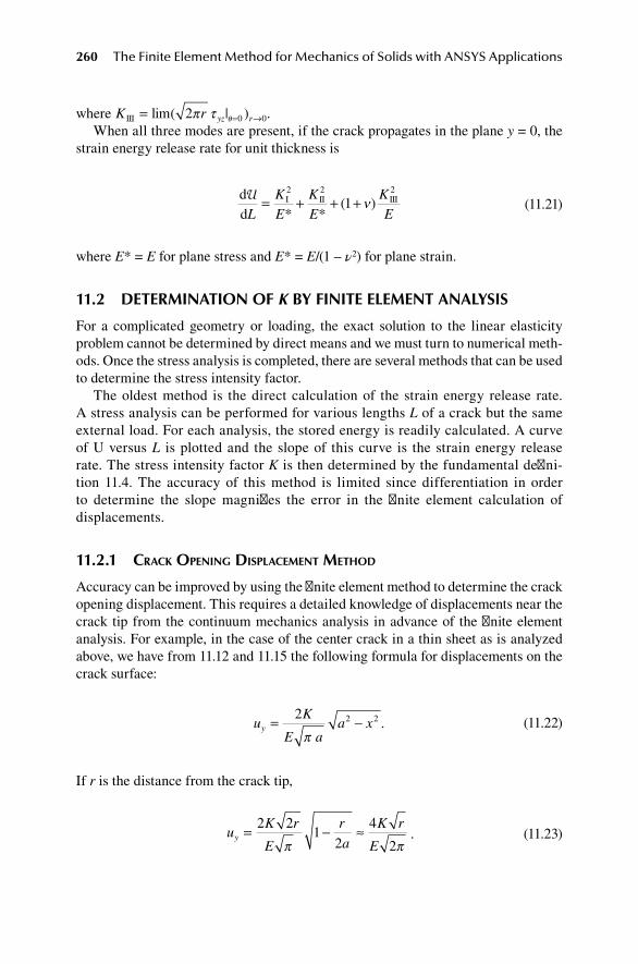
260 The Finite Element Method for Mechanics of Solids with ANSYS Applications
where K r yz rIII lim= = →( | )2 0 0π τ θ .When all three modes are present, if the crack propagates in the plane y = 0, the
strain energy release rate for unit thickness is
dd
I II IIIUL
KE
KE
KE
= + + +2 2 2
1* *
( )ν
(11.21)
where E* = E for plane stress and E* = E/(1 – ν2) for plane strain.
11.2 deterMInatIon of K By fInIte eleMent analySIS
For a complicated geometry or loading, the exact solution to the linear elasticity problem cannot be determined by direct means and we must turn to numerical meth-ods. Once the stress analysis is completed, there are several methods that can be used to determine the stress intensity factor.
The oldest method is the direct calculation of the strain energy release rate. A stress analysis can be performed for various lengths L of a crack but the same external load. For each analysis, the stored energy is readily calculated. A curve of U versus L is plotted and the slope of this curve is the strain energy release rate. The stress intensity factor K is then determined by the fundamental defini-tion 11.4. The accuracy of this method is limited since differentiation in order to determine the slope magnifies the error in the finite element calculation of displacements.
11.2.1 crack opening diSplaceMent Method
Accuracy can be improved by using the finite element method to determine the crack opening displacement. This requires a detailed knowledge of displacements near the crack tip from the continuum mechanics analysis in advance of the finite element analysis. For example, in the case of the center crack in a thin sheet as is analyzed above, we have from 11.12 and 11.15 the following formula for displacements on the crack surface:
uK
E aa xy = −2 2 2
π.
(11.22)
If r is the distance from the crack tip,
u
K r
E
r
a
K r
Ey = − ≈2 2
12
4
2π π. (11.23)
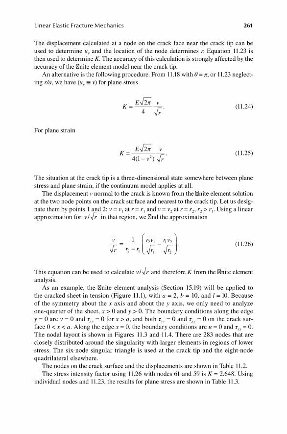
Linear Elastic Fracture Mechanics 261
The displacement calculated at a node on the crack face near the crack tip can be used to determine uy and the location of the node determines r. Equation 11.23 is then used to determine K. The accuracy of this calculation is strongly affected by the accuracy of the finite element model near the crack tip.
An alternative is the following procedure. From 11.18 with θ = π, or 11.23 neglect-ing r/a, we have (uy ≡ v) for plane stress
K
E
r
v= 24
π.
(11.24)
For plane strain
K
E
r
v=−2
4 1 2
πν( )
.
(11.25)
The situation at the crack tip is a three-dimensional state somewhere between plane stress and plane strain, if the continuum model applies at all.
The displacement v normal to the crack is known from the finite element solution at the two node points on the crack surface and nearest to the crack tip. Let us desig-nate them by points 1 and 2: v = v1 at r = r1 and v = v2 at r = r2, r2 > r1. Using a linear approximation for v r/ in that region, we find the approximation
v
r r r
r v
r
r v
r=
−−
1
2 1
2 1
1
1 2
2
.
(11.26)
This equation can be used to calculate v r/ and therefore K from the finite element analysis.
As an example, the finite element analysis (Section 15.19) will be applied to the cracked sheet in tension (Figure 11.1), with a = 2, b = 10, and l = l0. Because of the symmetry about the x axis and about the y axis, we only need to analyze one-quarter of the sheet, x > 0 and y > 0. The boundary conditions along the edge y = 0 are v = 0 and τxy = 0 for x > a, and both τyy = 0 and τxy = 0 on the crack sur-face 0 < x < a. Along the edge x = 0, the boundary conditions are u = 0 and τyx = 0. The nodal layout is shown in Figures 11.3 and 11.4. There are 283 nodes that are closely distributed around the singularity with larger elements in regions of lower stress. The six-node singular triangle is used at the crack tip and the eight-node quadrilateral elsewhere.
The nodes on the crack surface and the displacements are shown in Table 11.2.The stress intensity factor using 11.26 with nodes 61 and 59 is K = 2.648. Using
individual nodes and 11.23, the results for plane stress are shown in Table 11.3.

262 The Finite Element Method for Mechanics of Solids with ANSYS Applications
28 30 20 22 24 26 14
34 76 8185
80
75
18
36 8694
96
99
102126
128
38 90100
108
110
112
125
127 129 16
40 92 103113
115
117
42 93 106114
118
123
124122
74
44 91 104 111116
119
120
121
12 2
46 87 101 109107
98
95
79
10
48 8297 105
50 77 88 8984
736
32 53
83 78
55 57 598
fIgure 11.3 FEA nodes (corners only).
1 3 4 5 659 60 61 62
68
69
70
71
72
63
64 6566
67
fIgure 11.4 Nodes near the crack tip (node 1).
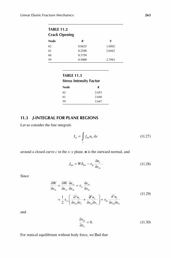
Linear Elastic Fracture Mechanics 263
11.3 J-Integral for plane regIonS
Let us consider the line integrals
I f n sm km k
c
= ∫ d
(11.27)
around a closed curve c in the x–y plane, n is the outward normal, and
f W
u
xkm km kjj
m
= −∂∂
δ τ .
(11.28)
Since
∂∂
= ∂∂
∂∂
= ∂∂
= ∂∂ ∂
+
W
x
W
x x
u
x x
m rs
rs
mrs
rs
m
rsr
m s
εε
τε
τ12
2 ∂∂∂ ∂
=
∂∂ ∂
2 2u
x x
u
x xs
m rkj
j
m k
τ
(11.29)
and
∂∂
=τ kj
kx0. (11.30)
For statical equilibrium without body force, we find that
taBle 11.2crack opening
node R V
62 0.0625 1.0502
61 0.2500 2.0442
60 0.3750
59 0.5000 2.7943
taBle 11.3 Stress Intensity factor
node K
62 2.653
61 2.646
59 2.647
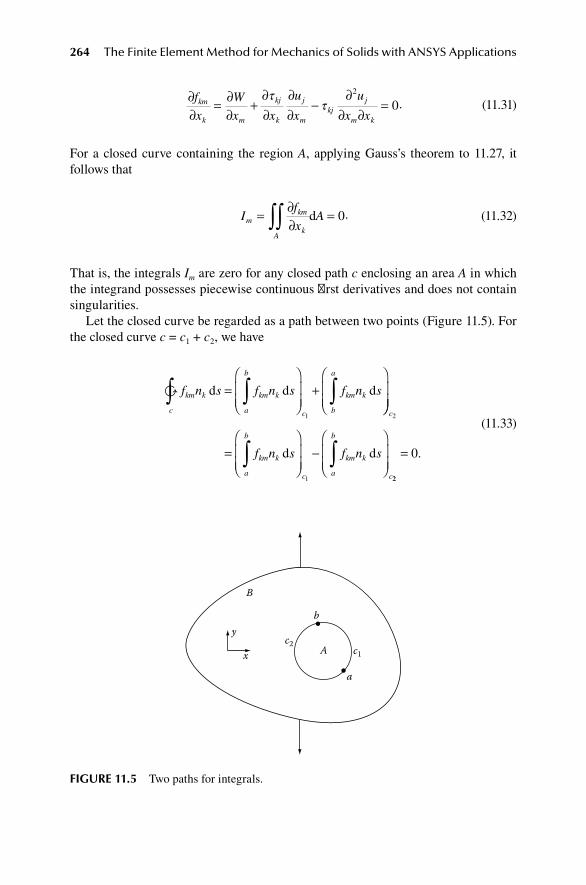
264 The Finite Element Method for Mechanics of Solids with ANSYS Applications
∂∂
= ∂∂
+∂∂
∂∂
−∂
∂ ∂=f
x
W
x x
u
x
u
x xkm
k m
kj
k
j
mkj
j
m k
ττ
2
0.
(11.31)
For a closed curve containing the region A, applying Gauss’s theorem to 11.27, it follows that
If
xAm
km
kA
= ∂∂
=∫∫ d 0.
(11.32)
That is, the integrals Im are zero for any closed path c enclosing an area A in which the integrand possesses piecewise continuous first derivatives and does not contain singularities.
Let the closed curve be regarded as a path between two points (Figure 11.5). For the closed curve c = c1 + c2, we have
f n s f n s f n skm k
c
km k
a
b
c
km k
b
a
d d d∫ ∫ ∫=
+
1
=
−
∫ ∫
c
km k
a
b
c
km k
a
b
c
f n s f n s
2
1
d d
22
0= .
(11.33)
x
y
B
c2c1A
a
b
fIgure 11.5 Two paths for integrals.

Linear Elastic Fracture Mechanics 265
Consequently,
f n s f n skm k
a
b
c
km k
a
b
c
d d∫ ∫
=
1 2
. (11.34)
That is, the integrals between two points are independent of the path between the points.
For an existing crack in plane stress or plane strain, we can choose the x axis parallel to the crack, and chose a path Γ starting and ending on the crack faces and enclosing a crack tip (Figure 11.6). The integral J = I1 is called the J-integral:3
J f n s
f Wu
x
k k
k k kjj
=
= −∂∂
∫ dΓ
,
δ τ11
.
(11.35)
We will show that J determines the energy release rate and therefore the stress inten-sity factors.
Recall that the integral is independent of the path. As a special case, we can choose the path Γ to be a circle of radius r about the crack tip and evaluate the J-integral as r → 0. In the limit, only the singular terms in stress and strain formulas for the stress near the crack tip will contribute to the expression for J. After lengthy calculations using Mathematica, one finds
cracky
B
L Γx
n
s
fIgure 11.6 J-integral path.

266 The Finite Element Method for Mechanics of Solids with ANSYS Applications
J
KE
KE
KE
= + + +I2
II III
* *( )
2 2
1 ν .
(11.36)
From 11.21, the J-integral is equal to the strain energy release rate:
J
L= ddU
. (11.37)
Numerical calculation of the J-integral from 11.35 requires one to identify a path, calculate U, Tk, and ∂uk/∂x along the path, and then integrate over the path. This is cumbersome in the context of the finite element analysis, and so a method has been devised to replace the line integral by integration over an area.4
Given a path Γ, construct a new path c surrounding it (Figure 11.7). Connect the two curves by paths along the crack surface, c+ and c–. For any smooth function q(x,y),
fqx
ax
qf qfx
a qf m skk
Ak
kk
kA
k k
∂∂
= ∂∂
− ∂∂
=∫ ∫d d d( )∂∂∫ ∫− ∂
∂A
k
kA
qfx
a
d ,
(11.38)
where m is the outward unit normal to A. First, we note that
∂∂
=f
xk
k
0. (11.39)
Next, the arbitrary function q(x,y) is given the values q = 1on Γ and q = 0 on c1. On c+ and c–, fk mk = 0. Finally, on Γ, m = –n. Thus,
B
y
xc+ c1c–
nm
nm Γ A
fIgure 11.7 Area integral method.

Linear Elastic Fracture Mechanics 267
fqx
a qf n s Jkk
A
k k
∂∂
= − = −∫ ∫d dΓ
(11.40)
or
J Wu
x
q
xak kj
j
kA
= − −∂∂
∂
∂∫ δ τ11
d .
(11.41)
The integral is evaluated over several element paths around the crack tip: J1 uses the first ring of elements (Figure 11.8), J2 uses the second ring, J3 uses the third ring, etc. Because of the finite element approximation, the value of J is different for each path. The first path for J1 is best discarded since it contains the singularity as a boundary. The true value for J is usually estimated as the average of the remaining paths.
J
nJ J Jn=
−+ + +1
1 2 3
(11.42)
11.4 proBleMS
1. Determine shape functions for a triangle with mid-side nodes from the eight-node quadrilateral by collapsing nodes 1, 4, and 8 together.
2. Given the shape functions for the four-node rectangle, obtain the shape functions for a right triangle by setting X1 = X4, Y1 = Y4, U1 = U4, and V1 = V4. Show that these shape functions agree with those for the three-node triangle if ξ = 2ζ2 + 2ζ3 – 1 and η = (ζ3 – ζ2)/(ζ3 + ζ2).
88
7868
69
5957
70
89
84
71
6665
6463
61674
72
61
path 1 path 2
8
path 3
7
fIgure 11.8 Element paths for J-integral evaluation.

268 The Finite Element Method for Mechanics of Solids with ANSYS Applications
3. For the singularity element (Section 5.9), given the shape functions 5.189
and the mapping 5.187, prove that yl= +4
1 2η ξ( ) for the triangular element
with quarter-point nodes (Figure 5.28). 4. Use ANSYS to determine the stress intensity factor for a center crack (a = 2)
in a 20 by 20 sheet assuming plane stress with E = 1, ν = 0.3, by the crack opening method. See Section 15.19.
5. Determine the stress intensity factor for problem 4 using the J-integral method. See Section 15.20.
referenceS
1. Tapley, B. D. (ed.), Eshback’s Handbook of Engineering Fundamentals, p. 478, Wiley, New York, 1990.
2. Liebowitz, H. (ed.) Fracture, Volume II, Mathematical Fundamentals, Academic Press, New York, 1968.
3. Rice, J. R., A path independent integral and the approximate analysis of strain concen-tration by notches and cracks, J. Appl. Mech., 35, 379–386, 1968.
4. Shih, C. F., B. Moran, and T. Nakamura, Energy release rate along a three-dimensional crack front in a thermally stressed body, Int. J. Fract., 30, 2, 79–102, 1986.
BIBlIography
Gdoutos, E. E., Fracture Mechanics, Springer, New York, 2005.Kanninen, M. F., and C. H. Popelar, Advanced Fracture Mechanics, Oxford Univ. Press,
London, 1985.
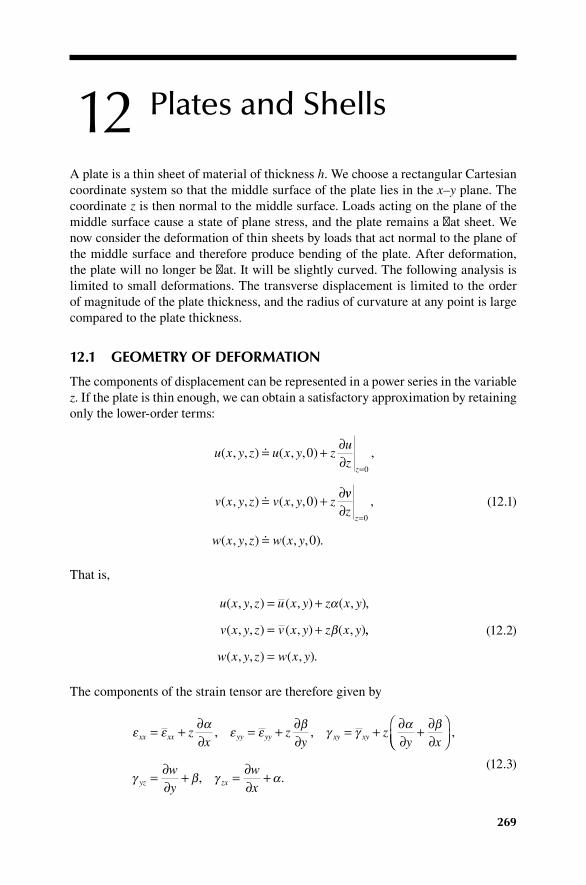
269
12 Plates and Shells
A plate is a thin sheet of material of thickness h. We choose a rectangular Cartesian coordinate system so that the middle surface of the plate lies in the x–y plane. The coordinate z is then normal to the middle surface. Loads acting on the plane of the middle surface cause a state of plane stress, and the plate remains a flat sheet. We now consider the deformation of thin sheets by loads that act normal to the plane of the middle surface and therefore produce bending of the plate. After deformation, the plate will no longer be flat. It will be slightly curved. The following analysis is limited to small deformations. The transverse displacement is limited to the order of magnitude of the plate thickness, and the radius of curvature at any point is large compared to the plate thickness.
12.1 geoMetry of deforMatIon
The components of displacement can be represented in a power series in the variable z. If the plate is thin enough, we can obtain a satisfactory approximation by retaining only the lower-order terms:
u x y z u x y zuz
v x y z v x y z
z
( , , ) ( , , ) ,
( , , ) ( , , )
0
0
0
+ ∂∂
+ ∂
=
vvz
w x y z w x y
z∂ =0
0
,
( , , ) ( , , ).
(12.1)
That is,
u x y z u x y z x y
v x y z v x y z x y
( , , ) ( , ) ( , ),
( , , ) ( , ) ( , )
= +
= +
α
β ,,
( , , ) ( , ).w x y z w x y=
(12.2)
The components of the strain tensor are therefore given by
ε εα
ε εβ
γ γα β
xx xx yy yy xy xyzx
zy
zy x
= + ∂∂
= + ∂∂
= + ∂∂
+ ∂∂
, ,
= ∂∂
+ = ∂∂
+
,
, .γ β γ αyz zx
wy
wx
(12.3)

270 The Finite Element Method for Mechanics of Solids with ANSYS Applications
The in-plane strains for z = 0 are
ε ε γxx yy xy
ux
vy
uy
vx
= ∂∂
= ∂∂
= ∂∂
+ ∂∂
, , .
(12.4)
The approximate expression 12.2 cannot be used to calculate εzz.
12.2 equatIonS of equIlIBrIuM
We will first calculate the stress resultants on cross sections of the plate along the coordinate lines.
The sign convention is shown in Figure 12.1. On the cross section normal to the x axis, the resultant forces and resultant moments about the axes per unit edge length are
N z N zx xx
h
h
xy xy
h
h
= =−
+
−
+
∫ ∫τ τd d/
/
/
/
2
2
2
2
, .
(12.5)
Q z M z z M z zx xz
h
h
x xx
h
h
xy xy= = =−
+
−
+
∫ ∫τ τ τd d d/
/
/
/
2
2
2
2
, ,−−
+
∫h
h
/
/
2
2
.
(12.6)
On the cross section normal to the y axis the resultant forces and resultant moments about the axes per unit edge length are
N z N zy yy
h
h
xy xy
h
h
= =−
+
−
+
∫ ∫τ τd d/
/
/
/
2
2
2
2
, .
(12.7)
Q z M z z M z zy yz
h
h
y yy
h
h
yx xy= = =−
+
−
+
∫ ∫τ τ τd d d/
/
/
/
2
2
2
2
, ,−−
+
∫h
h
/
/
2
2
.
(12.8)
x
z
y
Mxy
Mxy
My
Mx
QyQx
pz
fIgure 12.1 Plate sign convention.

Plates and Shells 271
The condition of equilibrium of an infinitesimal segment dx by dy of the plate evi-dently requires the stress resultants to satisfy the following differential equations. From a summation of forces in the x and y directions, we find
∂∂
+∂
∂+ =
∂∂
+∂
∂+ =
N
x
N
yp
N
y
N
xp
x xyx
y xyy
0
0
,
.
(12.9)
From a summation of forces in the z direction and a summation of moments about the x and y axes, we find
∂∂
+∂
∂+ =
∂∂
+∂
∂− =
∂∂
+∂
∂
Qx
Q
yp
Mx
M
yQ
M
y
M
x
x yz
x xyx
y xy
0
0
,
,
−− =Qy 0.
(12.10)
The applied loads per unit of plate area are px, py, and pz. The set 12.9 is the inte-grated equations of the theory of plane stress for in-plane loading of the sheet. The system 12.10 is associated with the bending of the plate.
12.3 conStItutIve relatIonS for an elaStIc MaterIal
Since the plate is thin, the stress component τzz is of the order of magnitude of the load-ing on the exterior surfaces of the sheet and much smaller than the primary stresses in bending τxx and τyy. It can be neglected in the stress–strain relations, so that
ε τ ντ ε τ ντxx xx yy yy yy xxE E
1 1( ), ( ).− −
(12.11)
Therefore,
τν
ε νε τν
ε νε τxx xx yy yy yy xx xy
E E E=−
+ =−
+ =1 1 22 2
( ), ( ),(11
2 1 2 1
+
=+
=+
νγ
τν
γ τν
γ
),
( ),
( ).
xy
yz yz zx zx
E E
(12.12)
From 12.3, 12.5, 12.7, and 12.12, the in-plane stress resultants have the constitutive relations:
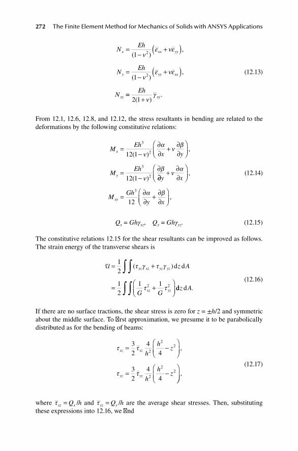
272 The Finite Element Method for Mechanics of Solids with ANSYS Applications
NEh
NEh
N
x xx yy
y yy xx
xy
=−
+( )
=−
+( )( )
,
( ),
1
1
2
2
νε νε
νε νε
==+
Ehxy2 1( )
.ν
γ
(12.13)
From 12.1, 12.6, 12.8, and 12.12, the stress resultants in bending are related to the deformations by the following constitutive relations:
MEh
x y
MEh
x
y
=−
∂∂
+ ∂∂
=−
∂
3
2
3
2
12 1
12 1
( ),
( )
να
νβ
νβ
∂∂+ ∂
∂
= ∂∂
+ ∂∂
y x
MGh
y xxy
να
α β
,
,3
12
(12.14)
Qx = Ghγxz, Qy = Ghγyz. (12.15)
The constitutive relations 12.15 for the shear resultants can be improved as follows. The strain energy of the transverse shears is
U = +
= +
∫∫12
12
1 12 2
( )τ γ τ γ
τ τ
xz xz yz yz
xz yz
z A
G G
d d
dd dz A∫∫ .
(12.16)
If there are no surface tractions, the shear stress is zero for z = ±h/2 and symmetric about the middle surface. To first approximation, we presume it to be parabolically distributed as for the bending of beams:
τ τ
τ τ
xz xz
yz yz
h
hz
h
hz
= −
= −
32
44
32
44
2
22
2
22
,
,
(12.17)
where τ xz xQ h= / and τ yz yQ h= / are the average shear stresses. Then, substituting these expressions into 12.16, we find

Plates and Shells 273
U = +
∫1
265
65
2 2hG
hG
Axz yzτ τ d .
(12.18)
We now require that the strain energy of the plate be accurately given by expression 12.16 but using the average shear stress and the strains at z = 0:
U = +( )
= +( )∫∫1
2
12
τ γ τ
τ γ τ γ
γxz xz yz yz
xz xz yz yz
z A
h h A
d d
d∫∫ .
(12.19)
This formula will agree with 12.18 if
τ γ τ γxz xz yz yzkG kG k= = =, , .
56
(12.20)
Therefore, the constitutive relations 12.15 become
Qx = kGhγxz, Qx = kGhγxz, (12.21)
where k is a shear correction factor, approximately 5/6. These relations are used in place of 12.15.
12.4 vIrtual Work
The complete set of equations for the bending part consists of the geometric relations from 12.3 combined with the constitutive relations 12.14 and 12.21,
Q kGhwx
Q kGhwy
MEh
x
y
x
= ∂∂
+
= ∂∂
+
=
α
β
,
,
(
3
12 11
12 1
2
3
2
−∂∂
+ ∂∂
=−
∂∂
+ ∂∂
να
νβ
νβ
να
),
( )
x y
MEh
y xy
=+
∂∂
+ ∂∂
,
( ),M
Ehy xxy
3
24 1 να β
(12.22)

274 The Finite Element Method for Mechanics of Solids with ANSYS Applications
and the equilibrium equations 12.10,
∂∂
+∂
∂+ =
∂∂
+∂
∂− =
∂∂
+∂
∂
Q
x
Q
yp
M
x
M
yQ
M
y
M
x
x yz
x xyx
y xy
0
0
,
,
−− =Qy 0,
(12.23)
where we drop the bar over the middle surface displacement w so that the bar can be used for virtual displacements.
The theorem of virtual work can be obtained by multiplying each equilibrium equation by a virtual displacement w and virtual rotations α and β and integrating over the area of the plate:
∂∂
+∂
∂+
+ ∂
∂+
∂∂
−
+
∂Qx
Q
yp w
Mx
M
yQ
Mx yz
x xyx α yy xy
yy
M
xQ A
∂+
∂∂
−
=∫ β d 0.
(12.24)
Integrating by parts gives
Qwx
Qwy
Mx
Myx y x xy
∂∂
+
+ ∂∂
+
+ ∂∂
+ ∂∂
+ ∂α β
α α β∂∂
+ ∂∂
= + +
∫
∫
xM
yA
p w A Q n Q n
y
A
z
A
x x y
βd
d yy x x xy y xy x y y
C
w M n M n M n M n s( ) + + + +{ }∫ ( ) ( )α β d .
(12.25)
The left-hand side is the internal virtual work of the stress resultants and the right-hand side is the external virtual work of the edge loads.
The virtual work formula shows that α is a rotation in the direction of Mx and β is a rotation in the direction of My. The positive directions are shown in Figure 12.1. Let θx = ROTX and θy = ROTY denote rotations about the respective axes with positive directions determined by the right-hand rule, then
θ β
θ α
x
y
= −
= +
,
.
(12.26)
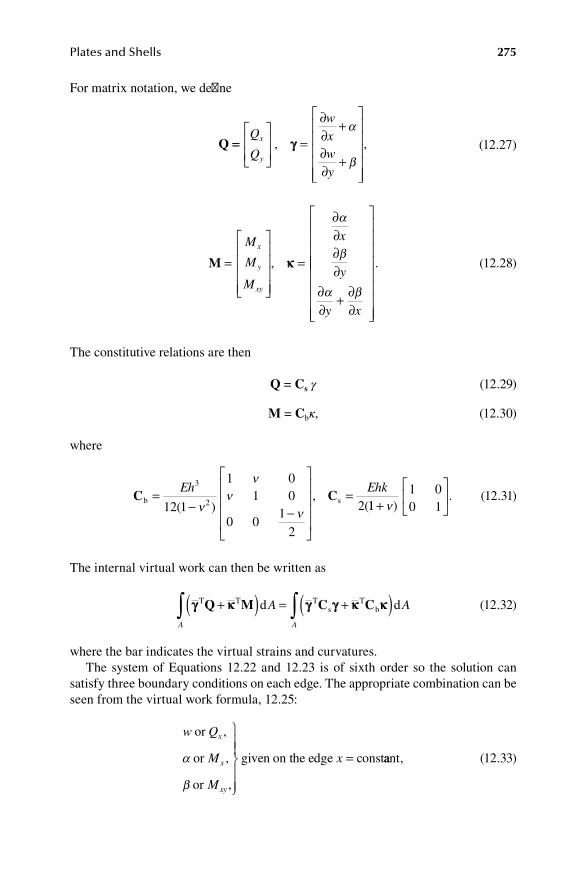
Plates and Shells 275
For matrix notation, we define
Q == γγQ
Q
wxwy
x
y
=
∂∂
+
∂∂
+
, ,α
β
(12.27)
M =
=
∂∂∂∂
∂∂
+ ∂∂
M
M
M
x
y
y x
x
y
xy
, .κκ
α
β
α β
(12.28)
The constitutive relations are then
Q = Cs γ (12.29)
M = Cbκ, (12.30)
where
C Cb s=− −
=Eh Ehk3
212 1
1 01 0
0 01
2
2( ),
(ν
νν
ν 111 00 1+
ν).
(12.31)
The internal virtual work can then be written as
γγ κκ γγ γγ κκ κκT T Ts
Tbd dQ M C C+( ) = +( )∫ ∫A A
A A
(12.32)
where the bar indicates the virtual strains and curvatures.The system of Equations 12.22 and 12.23 is of sixth order so the solution can
satisfy three boundary conditions on each edge. The appropriate combination can be seen from the virtual work formula, 12.25:
w Q
M
M
x
x
x
xy
or
or
or
given on the edge const
,
,
,
α
β
= aant,
(12.33)
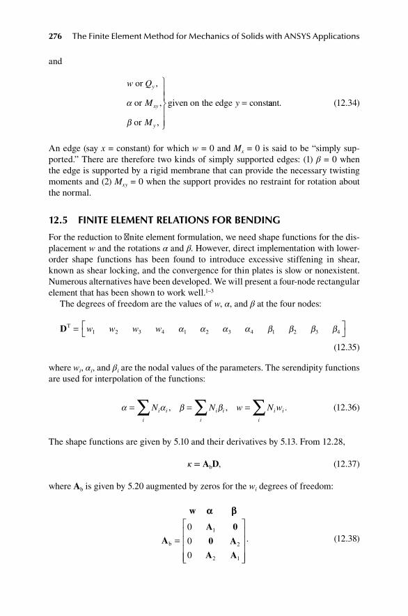
276 The Finite Element Method for Mechanics of Solids with ANSYS Applications
and
w Q
M
M
y
y
xy
y
or
or
or
given on the edge const
,
,
,
α
β
= aant.
(12.34)
An edge (say x = constant) for which w = 0 and Mx = 0 is said to be “simply sup-ported.” There are therefore two kinds of simply supported edges: (1) β = 0 when the edge is supported by a rigid membrane that can provide the necessary twisting moments and (2) Mxy = 0 when the support provides no restraint for rotation about the normal.
12.5 fInIte eleMent relatIonS for BendIng
For the reduction to finite element formulation, we need shape functions for the dis-placement w and the rotations α and β. However, direct implementation with lower- order shape functions has been found to introduce excessive stiffening in shear, known as shear locking, and the convergence for thin plates is slow or nonexistent. Numerous alternatives have been developed. We will present a four-node rectangular element that has been shown to work well.1–3
The degrees of freedom are the values of w, α, and β at the four nodes:
DT =
w w w w1 2 3 4 1 2 3 4 1 2 3 4α α α α β β β β
(12.35)
where wi, αi, and βi are the nodal values of the parameters. The serendipity functions are used for interpolation of the functions:
α α β β= = =∑ ∑ ∑N N w N wi i
i
i i
i
i i
i
, , .
(12.36)
The shape functions are given by 5.10 and their derivatives by 5.13. From 12.28,
κ = AbD, (12.37)
where Ab is given by 5.20 augmented by zeros for the wi degrees of freedom:
w
A
A 0
0 A
A A
αα ββ
b =
0
0
0
1
2
2 1
.
(12.38)
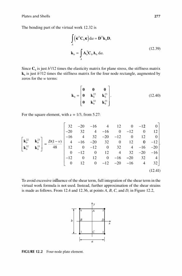
Plates and Shells 277
The bending part of the virtual work 12.32 is
κκ κκTb
Tb
b bT
b b
d
d
C D k D
k A C A
( ) =
=
∫
∫
a
a
A
A
,
.
(12.39)
Since Cb is just h3/12 times the elasticity matrix for plane stress, the stiffness matrix kb is just h3/12 times the stiffness matrix for the four node rectangle, augmented by zeros for the w terms:
k0 0 00 k k
0 k kb b b
b b
=
22 23
32 33
. (12.40)
For the square element, with ν = 1/3, from 5.27:
k k
k kb b
b b
D22 23
32 33
148
32 20 16 4 12 0 1
= −
− − −
( )ν
22 020 32 4 16 0 12 0 1216 4 32 20 12 0 12 04 16 20 32 0 12
− − −− − −
− − 00 1212 0 12 0 32 4 16 200 12 0 12 4 32 20 16
12 0 12 0 16
−− − −
− − −− − −−
− − −
20 32 40 12 0 12 20 16 4 32
.
(12.41)
To avoid excessive influence of the shear term, full integration of the shear term in the virtual work formula is not used. Instead, further approximation of the shear strains is made as follows. From 12.4 and 12.36, at points A, B, C, and D, in Figure 12.2,
1 2
34
x
y
a
b
A
B
C
D
fIgure 12.2 Four-node plate element.

278 The Finite Element Method for Mechanics of Solids with ANSYS Applications
γα α
γα α
γ
xzA
xzC
yzD
w w
a
w w
a
w w
= − + +
= − + +
= −
3 4 3 4
2 1 2 1
3
2
2
,
,
22 3 2
4 1 4 1
2
2
b
w w
byzB
+ +
= − + +
β β
γβ β
,
.
(12.42)
The shear for the element is now interpolated linearly between the two opposite points:
γ η γ η γ
γ ξ γ
xz xzA
xzC
yz yzD
= + + −
= + +
12
112
1
12
112
( ) ( ) ,
( ) (11 − ξ γ) .yzB
(12.43)
Combining these formulas, we have the representation for the shears:
γ = AsD, (12.44)
where
AsT =
− − − −+ − − ++ + +
12
1 1
1 1
1 1
ab
b a
b a
b a
( ) ( )
( ( )
( ) (
)
η ξ
η ξ
η ++− + + −
−
−
+
ξ
η ξ
η
η
η
)
( ) ( )
( )
( )
( )
b a
ab
ab
ab
ab
1 1
21 0
21 0
21 0
221 0
02
1
02
1
02
1
02
1
( )
( )
( )
( )
( )
+
−
+
+
−
η
ξ
ξ
ξ
ξ
ab
ab
ab
ab
w
w
w
w
1
2
3
4
1
2
3
4
1
2
3
4
α
α
α
α
β
β
β
β
.
(12.45)

Plates and Shells 279
The same interpolations are used for the virtual displacements. From the virtual work formula 12.32, the shear part of the stiffness matrix for the element is given by
k A C A
w
k k k
k k k
k
s sT
s s
s s s
s s s
s
d d=
=
∫ x yA
αα ββ11 12 13
21 22 23
311 32 33k ks s
,
(12.46)
where
ks11
2 2 2 2 2 2 2 2
48 1
8 8 4 8 4 4 8 4
=+
+ − − − − +Ehk
ab
a b a b a b a b
( )ν44 8 8 8 8 4 4 4
4 4 8 4
2 2 2 2 2 2 2 2
2 2 2 2
a b a b a b a b
a b a b
− + − + − −− − − + 88 8 4 8
8 4 4 4 4 8 8 8
2 2 2 2
2 2 2 2 2 2 2 2
a b a b
a b a b a b a b
+ −− + − − − +
,
(12.47)
ks21
48 1
4 4 2 24 4 2 22 2 4 42 2 4 4
=+
− −− −− −− −
Ehkb
( )ν
= ( )ksT12 , (12.48)
ks21
48 1
4 4 2 24 4 2 22 2 4 42 2 4 4
=+
− −− −− −− −
Ehkb
( )ν
= ( )ks
T12 , (12.49)
ks31
48 1
4 2 2 42 4 4 22 4 4 24 2 2 4
=+
− −− −− −− −
Ehka
( )ν
= ( )ksT13 , (12.50)
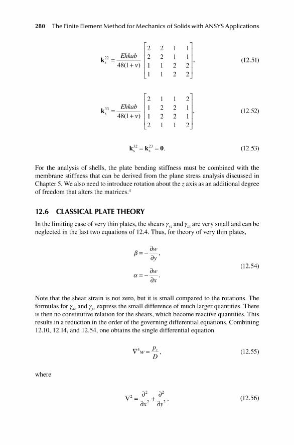
280 The Finite Element Method for Mechanics of Solids with ANSYS Applications
ks22
48 1
2 2 1 12 2 1 11 1 2 21 1 2 2
=+
Ehkab
( )ν, (12.51)
ks33
48 1
2 1 1 21 2 2 11 2 2 12 1 1 2
=+
Ehkab
( )ν, (12.52)
k k 0s s32 23= = . (12.53)
For the analysis of shells, the plate bending stiffness must be combined with the membrane stiffness that can be derived from the plane stress analysis discussed in Chapter 5. We also need to introduce rotation about the z axis as an additional degree of freedom that alters the matrices.4
12.6 claSSIcal plate theory
In the limiting case of very thin plates, the shears γyz and γzx are very small and can be neglected in the last two equations of 12.4. Thus, for theory of very thin plates,
β
α
= − ∂∂
= − ∂∂
wy
wx
,
.
(12.54)
Note that the shear strain is not zero, but it is small compared to the rotations. The formulas for γxz and γyz express the small difference of much larger quantities. There is then no constitutive relation for the shears, which become reactive quantities. This results in a reduction in the order of the governing differential equations. Combining 12.10, 12.14, and 12.54, one obtains the single differential equation
∇ =4w
p
Dz ,
(12.55)
where
∇ = ∂
∂+ ∂
∂2
2
2
2
2x y.
(12.56)

Plates and Shells 281
Since 12.55 is a fourth-order partial differential equation, the solution can satisfy only two boundary conditions on each edge. The appropriate conditions can be found from the virtual work formula. Using 12.54, from 12.25 the virtual work of the edge forces is
Q n Q n w M n M nwx
M n M nwyx x y y x x xy y xy x y y+( ) − + ∂
∂− + ∂
∂
( ) ( )
∫ ds
C
.
(12.57)
On the side where x is constant, ny = 0, nx = 1, ds = dy, the virtual work of the edge forces is
Q w Mwx
Mwy
y
Q w Mwx y
M
x x xy
y
y
x x
a
b
− ∂∂
− ∂∂
= − ∂∂
− ∂∂
∫ d
xxyxy
y
y
xxy
wM
yw y
QM
y
a
b
( ) +∂
∂
= +∂
∂
∫ d
ww Mwx
y M wx
y
y
xy y
y
a
b
a
b− ∂∂
− ∫ d .
(12.58)
Therefore, the appropriate boundary conditions are
w V QMxy
y
wx
M
x x
x
or
and
or
given on the ed
≡ + ∂∂
∂∂
gge constantx = , (12.59)
and
w V QMxy
x
wy
M
y y
y
or
and
or
given on the ed
≡ + ∂∂
∂∂
gge constanty = .
(12.60)
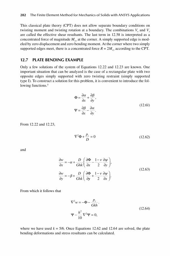
282 The Finite Element Method for Mechanics of Solids with ANSYS Applications
This classical plate theory (CPT) does not allow separate boundary conditions on twisting moment and twisting rotation at a boundary. The combinations Vx and Vy are called the effective shear resultants. The last term in 12.58 is interpreted as a concentrated force of magnitude Mxy at the corner. A simply supported edge is mod-eled by zero displacement and zero bending moment. At the corner where two simply supported edges meet, there is a concentrated force R = 2Mxy according to the CPT.
12.7 plate BendIng exaMple
Only a few solutions of the system of Equations 12.22 and 12.23 are known. One important situation that can be analyzed is the case of a rectangular plate with two opposite edges simply supported with zero twisting restraint (simply supported type I). To construct a solution for this problem, it is convenient to introduce the fol-lowing functions.5
Φ
Ψ
= ∂∂
+ ∂∂
= ∂∂
− ∂∂
α β
β α
x y
x y
,
.
(12.61)
From 12.22 and 12.23,
∇ + =2 0Φ p
Dz
(12.62)
and
∂∂
= − + ∂∂
− − ∂∂
∂∂
= − + ∂∂
wx
DGhk x y
wy
DGhk
αν ψ
β
Φ
Φ
12
,
yy x+ − ∂
∂
12
ν ψ.
(12.63)
From which it follows that
∇ = − −
− ∇ =
2
22
100
wp
Gkh
h
zΦ
Ψ Ψ
.
,
(12.64)
where we have used k = 5/6. Once Equations 12.62 and 12.64 are solved, the plate bending deformations and stress resultants can be calculated.

Plates and Shells 283
As an example, we consider a uniform load p on the rectangular plate with edge conditions as shown in Figure 12.3:
w
M
x
x
=
=
=
=
0
0
0
,
,
,
,β on the edge constant
(12.65)
and
w
M
M
yy
xy
=
=
=
=
0
0
0
,
,
,
,on the edge constant
(12.66)
corresponding to the two sets of conditions that may be called simply supported.The uniform load of magnitude p can be represented by a Fourier sine series in
the x direction:
p p x p
pn
naz n
n
n= = =∑ sin( ), , .ωπ
ω π4
(12.67)
Then, a solution can be constructed by series expansions:
w = 0
w = 0
w = 0
My = 0
Mx = 0
My = 0
Mxy = 0
Mxy = 0
a
β = 0
w = 0Mx = 0β = 0
b
y
x
fIgure 12.3 Plate with mixed boundary conditions.

284 The Finite Element Method for Mechanics of Solids with ANSYS Applications
w x y W y x
x y F y x
x
n
n
n
n
( , ) ( )sin( ),
( , ) ( )sin( ),
(
=
=
∑∑
ω
ωΦ
Ψ ,, ) ( )cos( ).y G y xn
n
= ∑ ω
(12.68)
Omitting the subscript n, we easily find a solution for each component of the load in terms of hyperbolic functions:
F c y c yp
D
W c y c yc
n= + +
= + −
1 2 2
3 4
Ch Sh
Ch Sh
( ) ( ) ,
( ) ( )
ω ωα
ω ω 11 24
2 2
2 21
5 1ωω
ωω
ωω
νy y
cy y
p
D
hnSh Ch( ) ( )( )
− + +−
,,
( ) ( ), .G c y c yh
= + = +
5 6
2 22 2
110
Ch Shγ γ γ ωω
(12.69)
Because of the symmetry about the x axis, we need to retain only the following terms:
F c yp
D
W c yc
y yp
D
n
n
= +
= − + +
1 2
31
421
Ch
Ch Sh
( ) ,
( ) ( )
ωω
ωω
ωω
ωων
γ
2 2
6
5 1h
G c y
( ),
( ).
−
= Sh
(12.70)
The three constants are determined by the conditions on y = 0. The expressions are rather lengthy so I will not reproduce them here.
This problem was solved for a = b by finite element method (FEM) (Section 15.26). We only need to use one-quarter of the plate with support conditions as shown in Figure 12.4. A uniform 20 × 20 mesh for the one-quarter was used. The calculated displacement at the center of the plate for h/a = 0.1, compared to the thin-plate approximation (CPT) and the exact solution of the shear the-ory using 400 terms in the series expansion, is shown in Table 12.1. The sup-port reaction qx/(pa) on the edge x = 0 is shown in Figure 12.5. The support

Plates and Shells 285
reaction qy/(pa) on the edge y = 0, compared to the exact solution, is shown in Figure 12.6.
The finite element results are for the centroid of the element (y/a = 0.0125) and the exact solution is for y = 0. Note there is a large negative Qy force near the cor-ner. This is the accurate description of the reaction represented by the concentrated corner force in the CPT. In addition to the force Qy, the support mechanism at this edge must provide a twisting moment Mxy/(pa2) as shown in Figure 12.7. The CPT
ROTX = 0
ROTY= 0
ROTY = 0
p = 1w = 0Mxy = 0
w = 0
yx
fIgure 12.4 One-quarter of a plate with mixed boundary conditions.
taBle 12.1 center displacement
exact feM cpt
wD
pa4610× 4456 4450 4060
0
0.05
0.1
0.15
0.2
0.25
0.3
0.35
0.4
0 0.05 0.1 0.15 0.2 0.25 0.3 0.35 0.4 0.45 0.5
Qx/
pa
Y/a
FEAexact
fIgure 12.5 Shear resultant along edge with zero twisting moment.

286 The Finite Element Method for Mechanics of Solids with ANSYS Applications
resolves this combination of reactions into the effective shear reaction Vy and the corner reaction R.
Version 12 of ANSYS recommends the four-node element SHELL181 and the eight-node element SHELL281, which allow large deformations, plasticity, and vis-coelasticity. Older versions of ANSYS offer several plate bending elements (43, 63, 93, 143). Table 12.2 shows the results using element SHELL181 for h/a =0.1 and a 20 × 20 mesh over one-quarter of the plate. Values of the stress resultants are at the element centroid. Maximum values are shown, except for the negative value of shear near the corner on the side with zero twisting rotation. SHELL181a uses the full integration option with incompatible modes. SHELL181b uses the reduced integra-tion option.
–1.2
–1
–0.8
–0.6
–0.4
–0.2
0
0.2
0.4
0 0.05 0.1 0.15 0.2 0.25 0.3 0.35 0.4 0.45 0.5
Qy/
pa
X/a
FEAQy/pa
fIgure 12.6 Shear resultant along edge with zero rotation.
00.5
11.5
22.5
33.5
44.5
5
0 0.05 0.1 0.15 0.2 0.25 0.3 0.35 0.4 0.45 0.5X/a
FEAMxy/pa2
Mxy
/pa2
fIgure 12.7 Twisting moment along edge with zero rotation.

Plates and Shells 287
12.8 proBleMS
1. Derive the virtual work formula 12.25 for bending of plates. Note that
∂∂
= ∂∂
=∫ ∫ ∫ ∫fx
a fn sfy
a fn sA
x
c A
y
c
d d d d,
.
(12.71)
2. Use ANSYS, SHELL281, to determine the deflection at the center for a uni-formly loaded square plate with clamped edges for a = b = 20, h = 1, ν = 0.3, D = 100, so that E = 10.92. Use 1/4 of the plate and symmetry conditions. Submit element layout, maximum deflection, maximum and minimum val-ues of moments and shears, and plot of QY for the clamped edge y = 0. See Section 15.27.
3. Solve the plate bending problem shown in Figure 12.8 using a 10 × 10 grid over one-quarter of the plate and symmetry conditions. See Section 15.26. Use a = b = 10, h = 1, ν = 0.3, D = 1, so that E = 10.92. Submit:(a) Maximum UZ and the (x,y) location.(b) Maximum and minimum values of QY and (x,y) location.(c) Graph of QY along line y = 0.
4. Use ANSYS to analyze a cylindrical shell roof under gravity loading (Figure 12.9).
taBle 12.2comparison of plate elements
Shell181aat centroid
Shell181bat centroid
exactat the edge
wD
pa4610×
4,451 4,450 4,456
M
pax2
510×4,909 4,908 4,919
M
pay
2510×
4,971 4,970
M
paxy
2510×
2,968 2,967
Qpa
x ×1043,740 3,740
Q
pay ×104
+3,331−7,108
+3,331−7,108
+3,455−10,700
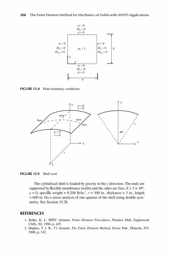
288 The Finite Element Method for Mechanics of Solids with ANSYS Applications
The cylindrical shell is loaded by gravity in the y direction. The ends are supported by flexible membranes (walls) and the sides are free, E = 3 × 10⁶, ν = 0, specific weight = 0.208 lb/in.3, r = 300 in., thickness = 3 in., length = 600 in. Do a stress analysis of one-quarter of the shell using double sym-metry. See Section 15.28.
referenceS
1. Bathe, K. J., MITC element, Finite Element Procedures, Prentice Hall, Englewood Cliffs, NJ, 1996, p. 425.
2. Hughes, T. J. R., T1 element, The Finite Element Method, Dover Pub., Mineola, NY, 2000, p. 342.
x
r
40°
y
x
y
z
L
v = 0u = 0
v = 0u = 0
symsymfree
free
fIgure 12.9 Shell roof.
w = 0pz = 1
w = 0
Mx = 0
My = 0
Mxy = 0
w = 0Mx = 0
Mxy = 0b
α = 0
w = 0My = 0α = 0
a
x
y
fIgure 12.8 Plate boundary conditions.

Plates and Shells 289
3. Zienkiewicz, O. C., and R. L. Taylor, The Finite Element Method for Solid and Structural Mechanics, Elsevier, New York, 2005, 6th ed., p. 397.
4. MacNeal, R. H., and R. L. Harder, A refined four-noded membrane element with rota-tional degrees of freedom, Comput. Struct., 28 (1), 75–84, 1988.
5. Marguerre, K., and H.-T. Woernle, Elastic Plates, Blaisdell Pub. Co., New York, 1969.
BIBlIography
Bathe, K. J., Finite Element Procedures, Prentice-Hall, Englewood Cliffs, NJ, 1996.Cook, R. D., D. S. Malkus, M. E. Plesha, and R. J. Witt, Concepts and Applications of Finite
Element Analysis, 4th ed., John Wiley & Sons, New York, 2002.

291
13 Large Deformations
13.1 theory of large deforMatIonS
Let us select one known configuration of the body as a reference configuration in which the body occupies a known region R of space.* This can be the configuration at any time. We will use a single rectangular Cartesian coordinate system. Let Xk denote the position of a particle in the reference configuration. In a deformed con-figuration r(t) at time t, this particle occupies a position xk. The motion relative to the fixed reference configuration is described by the mapping:
xk = xk(X,t). (13.1)
The velocity of a particle is
v
xtk
k= ∂∂
.
(13.2)
The acceleration of a particle is
a
vtk
k= ∂∂
.
(13.3)
The tensor G with components
G
xXkm
k
m
= ∂∂
(13.4)
is called the deformation gradient.† The law of conservation of mass is
ρρ0 = =G Jij .
(13.5)
The balance of momentum applied to an element of the deformed body gives‡
* For a complete treatment of the general theory, see Dill: Chapter 2. Refer to Preface.† We use here G for gradient in place of the more common F, which is reserved for force.‡ Throughout this section, the summation convention applies to repeated indices and their range is
1, 2, 3.
292 The Finite Element Method for Mechanics of Solids with ANSYS Applications
∂∂Tx
b a T Tkm
km m km mk+ = =ρ ρ , , (13.6)
where Tij are the components of the true (Cauchy) stress tensor. This formulation is not convenient for finite element calculations since the independent variables are the unknown coordinates xk of a particle in the unknown deformed position. A change of variables leads to the more convenient form of balance of momentum:
∂∂P
Xb amk
km m+ =ρ ρ0 0 , (13.7)
where
P G T T G Pji ik kj rm ri mi= =−ρ
ρρ
ρ0
0
1 , . (13.8)
The new tensor P is usually called the first Piola–Kirchhoff tensor.* Note that the derivatives are now with respect to the coordinates of position in the reference con-figuration, which are known quantities.
13.1.1 Virtual work
If we multiply 13.7 by arbitrary functions ϕm(X), called virtual displacements, and integrate over the reference configuration, we have†
∂∂PX
b a Vmk
km m m+ −
=∫ ρ ρ φ0 o dR
0.
(13.9)
Integration by parts yields
PX
V p A b a Vmkm
km m m m m
∂∂
= + −∫ ∫ ∫∂
φφ ρ ρ φd d d0 0
R R R
( ) , (13.10)
where the vector
pm = PmkNk (13.11)
is the surface traction per unit area of the reference configuration and N is the unit normal to the reference surface. This gives a physical interpretation for the Piola ten-
* P is the transpose of the Piola tensor in my book on continuum mechanics.† The more usual notation is ϕm = δxm.

Large Deformations 293
sor P: Pij is the jth component of the traction per unit undeformed area acting on the deformed surface that was the ith coordinate surface in the undeformed body.
Equation 13.10 is the virtual work formula for large deformations. The balance of momentum is satisfied if and only if this relation holds for all smooth functions ϕm(X). In order to complete the theory, we need the specific constitutive relation for the material. We will consider here only elastic materials at uniform temperature.
13.1.2 elaStic MaterialS
An elastic material is one for which the stress in the deformed configuration depends only on the local deformation in that configuration and not on the history of deforma-tion. Let the reference configuration be unstressed. The relation between stress and deformation must be such that the body remains stress-free in a rigid body motion. The general representation of such a relation is
T G f Gij ik km jm= ρ
ρ0
)(C , (13.12)
where
Cij = GkiGkj (13.13)
is the deformation tensor. Let us introduce the new tensor
S P G JG T G P G Sij mi jm ik km jm ki kj ij= = =− − −1 1 1, , (13.14)
which I will call the Kirchhoff tensor.* The constitutive relation then has a simple form
Sij = f(C)ij . (13.15)
Each function f defines a particular elastic material. We can show from thermo-dynamic considerations that f is the derivative of the strain energy with respect to the strain tensor E:
2Eij = Cij – δij, (13.16)
and†
S
WE
Wij
ij ij
= ∂∂
= ∂∂
( ) ( ).
C C2
C (13.17)
* S is what is often called the second Piola–Kirchhoff tensor; see Dill, p. 22. Refer to Preface.† Since Eij = Eji, the variables are not independent and care must be taken in evaluating the partial
derivatives; see Dill, p. 321. Refer to Preface.
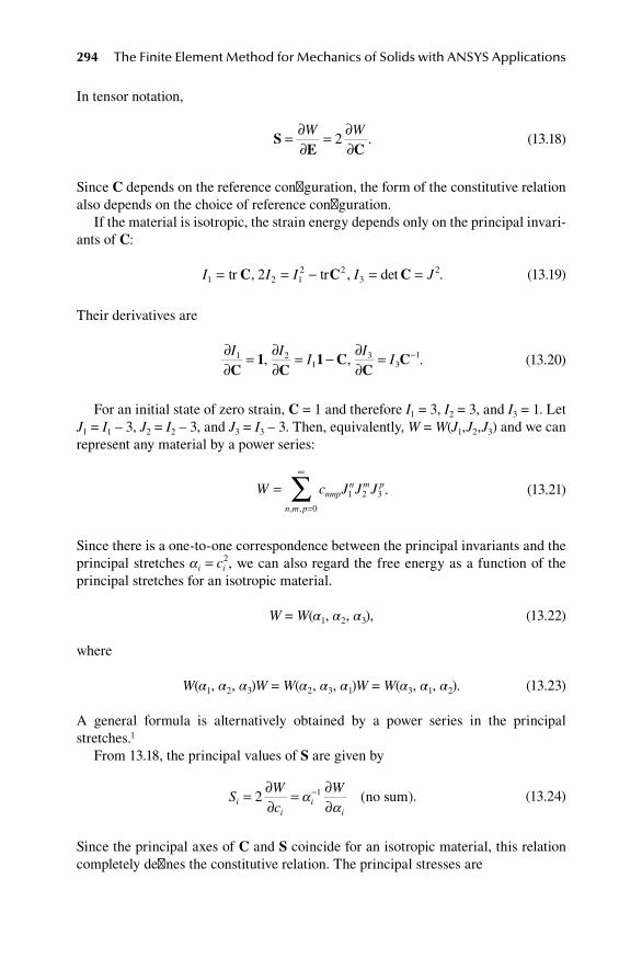
294 The Finite Element Method for Mechanics of Solids with ANSYS Applications
In tensor notation,
S
E C= ∂
∂= ∂
∂W W
2 . (13.18)
Since C depends on the reference configuration, the form of the constitutive relation also depends on the choice of reference configuration.
If the material is isotropic, the strain energy depends only on the principal invari-ants of C:
I I I I J1 2 12 2
322= = − = =tr trC C C, , det . (13.19)
Their derivatives are
∂∂
= ∂∂
= − ∂∂
= −I II
II1 2
13
31
C1
C1 C
CC, , . (13.20)
For an initial state of zero strain, C = 1 and therefore I1 = 3, I2 = 3, and I3 = 1. Let J1 = I1 – 3, J2 = I2 – 3, and J3 = I3 – 3. Then, equivalently, W = W(J1,J2,J3) and we can represent any material by a power series:
W c J J Jnmpn m p
n m p
==
∞
∑ 1 2 3
0, ,
. (13.21)
Since there is a one-to-one correspondence between the principal invariants and the principal stretches α i ic= 2, we can also regard the free energy as a function of the principal stretches for an isotropic material.
W = W(α1, α2, α3), (13.22)
where
W(α1, α2, α3)W = W(α2, α3, α1)W = W(α3, α1, α2). (13.23)
A general formula is alternatively obtained by a power series in the principal stretches.1
From 13.18, the principal values of S are given by
S
Wc
Wi
ii
i
= ∂∂
= ∂∂
−2 1αα
( )no sum . (13.24)
Since the principal axes of C and S coincide for an isotropic material, this relation completely defines the constitutive relation. The principal stresses are
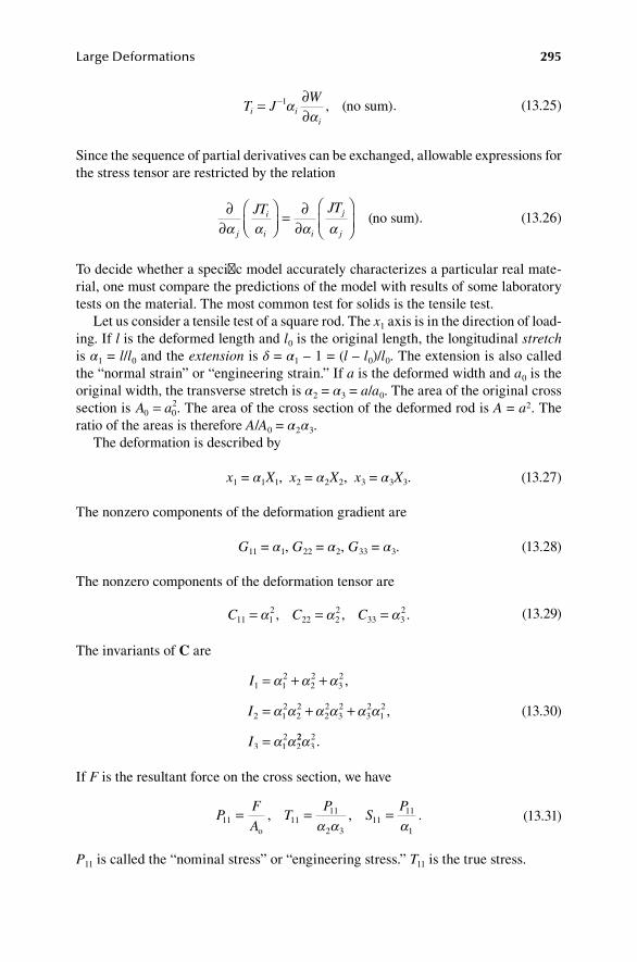
Large Deformations 295
T J
Wi i
i
= ∂∂
−1αα
, (no sum). (13.25)
Since the sequence of partial derivatives can be exchanged, allowable expressions for the stress tensor are restricted by the relation
∂∂
= ∂∂
α α α αj
i
i i
j
j
JT JT(no sum). (13.26)
To decide whether a specific model accurately characterizes a particular real mate-rial, one must compare the predictions of the model with results of some laboratory tests on the material. The most common test for solids is the tensile test.
Let us consider a tensile test of a square rod. The x1 axis is in the direction of load-ing. If l is the deformed length and l0 is the original length, the longitudinal stretch is α1 = l/l0 and the extension is δ = α1 – 1 = (l – l0)/l0. The extension is also called the “normal strain” or “engineering strain.” If a is the deformed width and a0 is the original width, the transverse stretch is α2 = α3 = a/a0. The area of the original cross section is A a0 0
2= . The area of the cross section of the deformed rod is A = a2. The ratio of the areas is therefore A/A0 = α2α3.
The deformation is described by
x1 = α1X1, x2 = α2X2, x3 = α3X3. (13.27)
The nonzero components of the deformation gradient are
G11 = α1, G22 = α2, G33 = α3. (13.28)
The nonzero components of the deformation tensor are
C C C11 12
22 22
33 32= = =α α α, , . (13.29)
The invariants of C are
I
I
I
1 12
22
32
2 12
22
22
32
32
12
3 12
2
= + +
= + +
=
α α α
α α α α α α
α α
,
,
2232α .
(13.30)
If F is the resultant force on the cross section, we have
P
F
AT
PS
P11 11
11
2 311
11
1
= = =o
, , .α α α
(13.31)
P11 is called the “nominal stress” or “engineering stress.” T11 is the true stress.
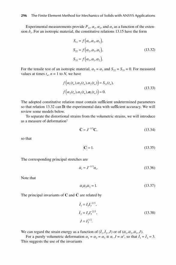
296 The Finite Element Method for Mechanics of Solids with ANSYS Applications
Experimental measurements provide P11, α1, α2, and α3 as a function of the exten-sion δ1. For an isotropic material, the constitutive relations 13.15 have the form
S f
S f
S f
11 1 2 3
22 2 3 1
33 3 1 2
= ( )= ( )= ( )
α α α
α α α
α α α
, , ,
, , ,
, , ..
(13.32)
For the tensile test of an isotropic material, α2 = α3 and S22 = S33 = 0. For measured values at times tn, n = 1 to N, we have
f t t t S t
f t t
n n n n
n n
α α α
α α
1 2 2 11
2 2
( ), ( ), ( ) ( ),
( ), ( ),
( ) =
αα1 0( ) .tn( ) =
(13.33)
The adopted constitutive relation must contain sufficient undetermined parameters so that relation 13.32 can fit the experimental data with sufficient accuracy. We will review some models below.
To separate the distortional strains from the volumetric strains, we will introduce as a measure of deformation2
C C= −J 1 3/ , (13.34)
so that
C = 1. (13.35)
The corresponding principal stretches are
α αi iJ= −1 3/ . (13.36)
Note that
α α α1 2 3 1= . (13.37)
The principal invariants of C and C are related by
I I I
I I I
J I
1 1 31 3
2 2 32 3
31 2
=
=
=
−
−
/
/
/
,
,
.
(13.38)
We can regard the strain energy as a function of ( , , )I I J1 2 or of ( , , , )α α α1 2 3 J .For a purely volumetric deformation α1 = α2 = α3 ≡ α, J = α3, so that I I1 2 3= = .
This suggests the use of the invariants

Large Deformations 297
J I J I J J1 1 2 2 33 3 1= − = − = −, , , (13.39)
and expressing
W W J J J= ( , , )1 2 3 . (13.40)
Examples are given below.Any relation that applies to large deformations must also apply to small deforma-
tion gradients. From 13.4, we find*
G = 1 + H (13.41)
where H is the displacement gradient. For small deformations
H = O( )ε (13.42)
where ε << 1. The small strain tensor is defined by
εε == 1
2H H+( )T .
(13.43)
Up to first order,
C 1
E C 1
P S T
+
= −
2
12
εε
εε
,
( )
.
,
(13.44)
For the tensile test, αi = 1 + εi, where εi << 1, α εi i2 1 2 + , etc. The invariants of C
are approximately
I1 ≐ 3 + 2tr ε, I2 ≐ 3 + 4tr ε, I3 ≐ 1 + 2tr ε. (13.45)
And tr ε = ε1 + ε2 + ε3 is the volumetric strain.
13.1.3 Mooney–riVlin Model of an incoMpreSSiBle Material
In this case, the material is modeled as incompressible, that is, ρ = ρ0 and the mean stress is determined by that constraint, rather than a constitutive relation. The Mooney–Rivlin relation is most compactly stated directly in terms of the true stress tensor. With respect to a stress-free reference configuration,
* We use here the standard matrix notation: for example, G = [Gkm], where k is the row index and m is the column index.
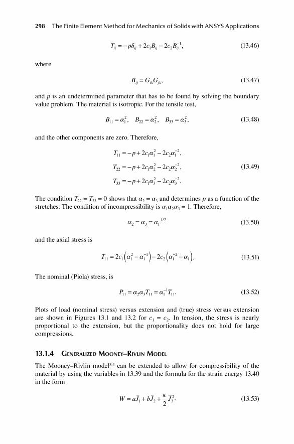
298 The Finite Element Method for Mechanics of Solids with ANSYS Applications
T p c B c Bij ij ij ij= − + − −δ 2 21 21, (13.46)
where
Bij = GikGjk, (13.47)
and p is an undetermined parameter that has to be found by solving the boundary value problem. The material is isotropic. For the tensile test,
B B B11 12
22 22
33 32= = =α α α, , , (13.48)
and the other components are zero. Therefore,
T p c c
T p c c
T
11 1 12
2 12
22 1 22
2 22
33
2 2
2 2
= − + −
= − + −
−
−
α α
α α
,
,
== − + − −p c c2 21 32
2 32α α .
(13.49)
The condition T22 = T33 = 0 shows that α2 = α3 and determines p as a function of the stretches. The condition of incompressibility is α1α2α3 = 1. Therefore,
α α α2 3 11 2= = − /
(13.50)
and the axial stress is
T c c11 1 1
211
2 12
12 2= −( ) − −( )− −α α α α . (13.51)
The nominal (Piola) stress, is
P T T11 2 3 11 11
11= = −α α α . (13.52)
Plots of load (nominal stress) versus extension and (true) stress versus extension are shown in Figures 13.1 and 13.2 for c1 = c2. In tension, the stress is nearly proportional to the extension, but the proportionality does not hold for large compressions.
13.1.4 generalized Mooney–riVlin Model
The Mooney–Rivlin model3,4 can be extended to allow for compressibility of the material by using the variables in 13.39 and the formula for the strain energy 13.40 in the form
W aJ bJ J= + +1 2 3
2
2κ .
(13.53)

Large Deformations 299
From 13.17,
S = aA1 + bA2 + κ(J – 1)JC–1 (13.54)
where
AC
1 C
AC
11 2 3
11
22 2
2 213
2 2
= ∂∂
= −
= ∂∂
=
− −
−
IJ I
IJ
/
/
,
331 2
123
I I1 C C− −
− .
(13.55)
–6
–4
–2
0
2
4
6
–0.6 –0.4 –0.2 0 0.2 0.4 0.6 0.8 1
Load
Extension
fIgure 13.1 Load extension for tensile test of a Mooney–Rivlin material.
–6
–4
–2
0
2
4
6
–0.6 –0.4 –0.2 0 0.2 0.4 0.6 0.8 1
Stre
ss
Extension
fIgure 13.2 Stress extension for tensile test of a Mooney–Rivlin material.

300 The Finite Element Method for Mechanics of Solids with ANSYS Applications
The stress tensor is given by
J a b J J aI bIT B B 1= − + − − +
−2 2 113
213
211 2κ ( ) , (13.56)
where
B B= −J 2 3/ . (13.57)
If the material is incompressible, J = 1 and the stress–strain relation reduces to the incompressible form 13.46.
The principal stresses are
JT a I a I Jk k k= −
− −
+ −−2 1
32 1
311
21 2
22α α κ ( ). (13.58)
The volume change is modeled by the simple relation
p J≡ = −1
31tr ( )T κ . (13.59)
For the tensile test, loading along the x1 axis, α α2 3= and condition 13.37 gives
α α2 11 2= − / . From 13.58,
JT a b1 1
211
1 122 2= −( ) + −( )− −α α α α .
(13.60)
Equations 13.59 and 13.60 determine α1 and α2 for a given T1. For a = b = 25 and κ = 500, the solution is given in Table 13.1.
Figure 13.3 shows the stress–strain curve for the nominal stress, P1/a, versus the extension α1 – 1.
taBle 13.1Mooney–rivlin Model
T1 α1 α2 P1 J αα1
10 1.0364 0.9855 9.713 1.00667 1.03411
20 1.0744 0.9711 18.862 1.01333 1.06973
30 1.1141 0.9568 27.465 1.02000 1.10680
40 1.1554 0.9427 35.545 1.02667 1.14527
50 1.1980 0.9287 43.126 1.03333 1.18502
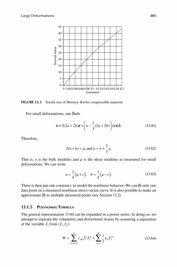
Large Deformations 301
For small deformations, one finds
ττ == εε εε2 2 2
13
2 2( ) ( ) ( )a b a b+ + − +
κ tr 1 . (13.61)
Therefore,
2
23
( ) ,a b+ = = +µ κ λ µand . (13.62)
That is, κ is the bulk modulus and μ is the shear modulus as measured for small deformations. We can write
a c b c= +( ) = −( )1
414
µ µ, .
(13.63)
There is then just one constant c to model the nonlinear behavior. We can fit only one data point on a measured nonlinear stress–strain curve. It is also possible to make an approximate fit to multiple measured points (see Section 13.2).
13.1.5 polynoMial forMula
The general representation 13.40 can be expanded in a power series. In doing so, we attempt to separate the volumetric and distortional strains by assuming a separation of the variable J3 from ( , )J J1 2 :
W c J J Jnm
n m
n m
N
nn
n
M
= += = =∑ ∑1 2
0
32
1
12
κ .
(13.64)
0
5
10
15
20
25
30
35
40
45
0 0.02 0.04 0.06 0.08 0.1 0.12 0.14 0.16 0.18 0.2Extension
Nor
mal
stre
ss
fIgure 13.3 Tensile test of Mooney–Rivlin compressible material.
302 The Finite Element Method for Mechanics of Solids with ANSYS Applications
From 13.18,
S A A= +
+
−
=
−
=
−
∑ ∑c nJ c nJ
c nJ J
nn
n
N
nn
n
N
nmn
0 11
1
1
0 21
2
1
11
2mm n m
m
N
n
N
nn
n
M
mJ J
n J J
A A
C
1 1 21
2
11
32 1 1
1
+( )
+
−
==
− −
=
∑∑
∑ κ ,,
(13.65)
where A1 and A2 are defined by 13.55. For N = 3 and M = 1,
S A= + + + + +( )+
c c J c J c J c J J c J10 11 2 20 1 30 12
21 1 2 12 22
12 3 2
cc c J c J c J c J J c J01 11 1 02 2 03 22
12 1 2 21 12
22 3 2+ + + + +( )+
A
κ JJ J−( ) −1 1C .
(13.66)
From 13.14, the true stress is
J c nJ c nJ
c nJ J
nn
n
N
nn
n
N
nmn
T A A= +
+
−
=
−
=
−
∑ ∑0 11
1
1
0 21
2
1
11
22 1 1 21
2
11
32 1
1
m n m
m
N
n
N
nn
n
M
mJ J
n J J
A A
1
+( )
+
−
==
−
=
∑∑
∑ κ ,
(13.67)
where
A B 1 B B
A B 1
12 3
21
2
223
223
= − =
= − +
−
−
, ,
.
J
I
/
(13.68)
For a purely volumetric strain: α1 = α2 = α3 = α, J = α3, J J1 2 0= = . In this case, from 13.67,
13
1 2 1
1
tr n Jnn
n
M
T = − −
=∑ κ ( ) . (13.69)

Large Deformations 303
The principal stress and principal stretches are related by
ˆ ˆT T c nJ c nJnn
n
N
nn
1 2 0 11
12
22
1
0 21
222 2− = −( ) +−
=
− −∑ α α α −−( )
+ −( ) +
−
=
− −
∑ α
α α α
12
1
11
2 12
12
1 212
n
N
nmn m n mc nJ J mJ J 22
21
2
11
− −
==
−( )( )∑∑ αm
N
n
N
,
(13.70)
ˆ ˆT T c nJ c nJnn
n
N
nn
2 3 0 11
22
32
1
0 21
322 2− = −( ) +−
=
− −∑ α α α −−( )
+ −( ) +
−
=
− −
∑ α
α α α
22
1
11
2 22
32
1 212
n
N
nmn m n mc nJ J mJ J 33
22
2
11
− −
==
−( )( )∑∑ αm
N
n
N
,
(13.71)
α α α1 2 3 1= . (13.72)
where T̂ T= J is the weighted, or Kirchhoff, stress measure.In terms of the constants cnm, the case N = 1 is known as the two-element model,
N = 2 as the five-element model, and N = 3 as the nine-element model. The two-element model with one volume term is identical to the compressible Mooney–Rivlin model (13.53). For the two-element model,
13
1tr JT = −κ ( )
(13.73)
for volumetric strain, and
ˆ ˆ ,T T c c1 2 10 1
222
01 22
122 2− = −( ) + −( )− −α α α α
(13.74)
ˆ ˆ ,T T c c2 3 10 2
232
01 32
222 2− = −( ) + −( )− −α α α α
(13.75)
for distortion.
13.1.6 ogden’S function
Using the reduced principal stretches 13.36, a possible polynomial expansion is Ogden’s potential:
W
aJi
i
a a a
i
N
k k
k
N
i i i= + + −( ) + −( )= =
∑ ∑µα α α
κ1 2 3
1
2
1
32
1
(13.76)

304 The Finite Element Method for Mechanics of Solids with ANSYS Applications
where μi, ai, and κk are the experimentally determined material constants. Applying this relation to the case of small deformations, we find that the shear modulus
µ µ==∑ ai i
i
N
1 and κ1 is the bulk modulus. The case a1 = 2 and a2 = –2 leads back to
the Mooney–Rivlin model. Since α α α1 2 3 1= ,
I2 1 2 2 3 3 1 12
22
32= + + = + +− − −α α α α α α α α α . (13.77)
Using only the first two terms of the series and one volume term, 13.25 gives
T J I J I Ik k k= −( ) − −( ) +− − − −µ α µ α κ1
5 3 21 2
1 3 22 3
11
13
13
/ / (JJ − 1). (13.78)
The small deformation shear modulus μ = μ1 + μ2 and κ1 is the bulk modulus.
13.1.7 Blatz–ko Model
The following constitutive relation for isothermal deformations of an isotropic elas-tic material was originally devised from experiments on polyurethane foam.5,6 The formula for the strain energy is
W
II
I= + −
µ2
2 52
33 .
(13.79)
Using 13.20, the stress–strain relations is found to be
S 1 C C= − + −
−µ
II I
III
1
3 33
2
3
11.
(13.80)
For small deformations, using 13.45 and S ≐ τ, the stress–strain relation is
τ = 2με + μ(tr ε)1. (13.81)
We see that μ is the shear modulus and the Poisson ratio is ν = 1/4, that is, λ = μ.To illustrate the behavior of this material, let us consider the tensile test. Using
13.29,
S I I I Ii i i i= − − +( )− − −µ α α α3
11
22
233 2 2/ . (13.82)
For a tensile test along the x axis, S2 = S3 = 0, and we find that
α α α α2 3 24
11= = −, . (13.83)

Large Deformations 305
It then follows that
S1 1
3 21
4= −( )− −µ α α/ . (13.84)
The true stress is
T11 1
5 21= −( )−µ α / .
(13.85)
The nominal stress (Piola tensor) is
P11 1
1 213= −( )− −µ α α/ .
(13.86)
Some calculated values are shown in Table 13.2.The results are plotted in Figure 13.4, where G denotes the shear modulus μ. The
material is not stable for large stretch: dS11/dα1 = 0 at α1 = 1.48. The model cannot
taBle 13.2Blatz–ko tensile test
α1 – 1 P11/μ
0 0
0.1 0.20215
0.2 0.33417
0.3 0.42189
0
0.1
0.2
0.3
0.4
0.5
0.6
0.7
0.8
0.9
1
1 1.5 2 2.5 3 3.5
Stre
ss m
easu
re
Stretch
T/G
S/G
P/G
fIgure 13.4 Stress vs. stretch for tensile test of Blatz–Ko model.

306 The Finite Element Method for Mechanics of Solids with ANSYS Applications
apply to a real material for greater stretches, and one can expect computational dif-ficulties if the Piola (nominal) stress approaches one-half of the shear modulus, or any stretch ratio approaches 1.5.
13.1.8 logarithMic Strain MeaSure
The logarithmic strain measure is defined as
e V n n= ==
∑ln( ) ( )ln α i i i
i 1
3
(13.87)
where (αi,ni) are the eigenvalues and eigenvectors of the left stretch tensor V = GGT. The constitutive relation
T = 2μe + λ tr(e)1 (13.88)
satisfies objectivity and describes an isotropic material. For a tensile test with true stress T11 = σ and extension α – 1,
σ/E = ln(α). (13.89)
This relation is linear up to three significant figures for 0 ≤ σ/E < 0.001. The rela-tion is nearly linear even for much larger extensions (Figure 13.5). This constitutive relation is used by ANSYS when the material model is specified as linear elastic isotropic and large displacement effects are enabled (NLGEOM ON).
0
0.1
0.2
0.3
0.4
0.5
0.6
0 0.1 0.2 0.3 0.4 0.5 0.6 0.7 0.8 0.9 1Extension
σ/E
fIgure 13.5 True stress vs. logarithmic strain.

Large Deformations 307
13.1.9 yeoh Model
Let us consider the series representation 13.64 but retain only the lower-order terms in I1:
W = a1(I1 – 3) + a2(I1 – 3)2 + a3(I1 – 3)3. (13.90)
An incompressible model with this strain energy function has been found to provide fit data on carbon black–filled rubber vulcanizates.7 In this case,
T 1 B= − + ∂
∂p
WI
21
.
(13.91)
In a simple shearing motion,
B = 1 + k(e1e2 + e2e1) + k2e1e1. (13.92)
The corresponding shear stress is
T12 = 2a1k + 4a2k3 + 6a3k5. (13.93)
For small deformations k is the shear strain, so the shear modulus is μ = 2a1. For filled rubber, the constant a2 is typically negative and the constant a3 is a small frac-tion of the shear modulus.
For the tensile test,
B e e e e e e= + +α α α12
1 1 22
2 2 32
3 3. (13.94)
The principal stresses are
T p a a I a Ii i= − + + − + −( )2 2 3 3 32
1 2 1 3 12α ( ) ( ) . (13.95)
Since α α α2 3 11 2= = − / for the incompressible model, we find from T2 = 0 that
T a a I a I1 1
21
11 2 1 3 1
22 2 3 3 3= − + − + −( )−( ) ( ) ( )α α . (13.96)
The Yeoh model can be extended to compressible materials by introducing the modified invariant I1 in place of I1 and choosing a model for volumetric strain such as
W a I b Jn
n
n
nn
n
= − + −∑ ∑( ) ( ) .123 1 (13.97)

308 The Finite Element Method for Mechanics of Solids with ANSYS Applications
From 13.18,
S 1 C= + − −
+ −
− −2 223
2 3
12 3
12
1 11
1
a J b J J I a
na In
/ ( )
( )) ( ) ( )n
n
nn
nnJ nb J J na I I− −
=
− −∑ + − − −1 2 3
2
2 11
112 1
23
3/ 1
=
−∑n 2
1C .
(13.98)
For small deformations J ≐ 1 + tr ε, I1 ≐ 3 + 2tr ε, I1 3 , C–1 ≐ 1 – 2ε,
S 1= + −
4 223
21 1 1a b aεε .
(13.99)
Therefore, the shear modulus μ = 2a1 and the bulk modulus κ = 2b1.
13.1.10 fitting conStitutiVe relationS to experiMental data
In practice, we begin with the results of material testing and we have to adjust the coefficients in the constitutive model to fit the measured data with adequate accu-racy. In principle, the polynomial formula 13.21 can fit any experiment, but in prac-tice we must truncate the series at some point and the determination of the remaining coefficients from the experimental data is difficult. ANSYS provides for direct input of experimental data and determination of the material parameters of the model to fit the data by a linear or nonlinear regression analysis. The minimum experimental test data needed to characterize the material are those from a tensile test and a volu-metric deformation.
13.1.10.1 volumetric dataThe measured data consist of the mean pressure p = –tr T/3 and the ratio J of deformed volume to undeformed volume. For example, for the polynomial model, from 13.73,
p n Jnn
n
M
= − − −
=∑ κ ( ) .1 2 1
1 (13.100)
The material constants κn are determined by fitting this formula to the measured curve of p versus J.
13.1.10.2 tensile testSuppose the x axis is the loaded direction; for an isotropic material, the coordinate axes are principal axes of stress and strain. The true stress is T1. The transverse stretches are equal, α2 = α3, and the ratio of deformed volume to initial volume is J = α α1 2
2. The
Large Deformations 309
nominal stress P1 is the load divided by the original area, P T J T1 22
1 11
1= = −α α and the Kirchhoff stress measure is T̂ JT1 1= . One measures α2, α1, and P1. This determines the stress–strain curve ˆ ( )T1 1 1versus α − . For example, for the polynomial model, from 13.70 with T̂2 0= and α α2 1
1 2= − / ,
T̂ c nJ c nJnn
n
N
nn
1 0 11
12
11
1
0 21
1 122 2= −( ) + −− −
=
− −∑ α α α α(( )
+ −( ) + −
=
− − −
∑n
N
nmn m n mc nJ J mJ J
1
11
2 12
11
1 21
1 12 α α α α −−
==
( )( )∑∑ 2
11 m
N
n
N
.
(13.101)
A curve fit to the tensile test data determines the material constants cnm.
13.1.10.3 Biaxial testA thin sheet is loaded by tension in two orthogonal directions in the plane of the sheet: T1 = T2, T3 = 0, α2 = α1. From 13.70–13.72 with α α1
23 1= ,
T̂ c c1 10 1
21
401 1
41
22 2= −( ) + −( )− − −α α α α . (13.102)
This test can be used in place of the tensile test or in addition to it.Examples are provided in Sections 15.37 and 15.38. If no volume data are entered,
ANSYS assumes an incompressible material (except for the Blatz–Ko model). The ANSYS program sometimes returns unrealistic values and must be used only as a starting point and with caution.
13.2 fInIte eleMentS for large dISplaceMentS
The equilibrium condition is expressed by the virtual work formula 13.10:
PX
V p A b Viji
ji i i i
∂∂
= +∫ ∫ ∫φφ ρ φd d d0
R R R∂
.
(13.103)
Integration is over the chosen reference configuration. In this section, the reference configuration is the unstressed initial body. We divide that configuration into finite elements and generate the variational function ϕ by using the shape functions for the elements:
φ φi iK K
K
i iK KN D N D= { } { } =∑ == ,, φφ ND,
(13.104)
where D denotes arbitrary (virtual) nodal displacements. The gradients of ϕ are

310 The Finite Element Method for Mechanics of Solids with ANSYS Applications
∂∂
= = ∂∂∑φi
jijK K
K
ijKiK
jXA D A
NX
, , (13.105)
or, arranging the gradient in a column matrix using the FORTRAN ordering,
∂∂
=
φ
φ
φ
φm
kX
1 1
2 1
3 1
,
,
,
.
.
.
= { } = = = + −A D A A i jK K K ijKα α αAD, , ( ).3 1
(13.106)
Since the virtual work formula 13.103 must hold for arbitrary DK, we find the follow-ing finite element version of the virtual work formula in matrix notation:
A P N p N bT T T0d d dV A V
m m mm m mR R R
∫∑ ∫∑ ∫∑= +∂ ∂
ρ , (13.107)
where the components of the Piola tensor P, the surface traction p per unit un deformed area, and the body force b per unit mass, are put into column matrices using the FORTRAN ordering: P = {Pα}, Pα = Pij, α = i + 3( j – 1).
The right-hand side of 13.107 is the usual matrix of given external nodal F forces at any time t. The left-hand side is the matrix of internal nodal forces f due to stresses that balance the external forces. Equation 13.107 therefore simply states that
f(t) = F(t), (13.108)
where
f A P( ) ( ) ,
( )
t t V
f A P t dV.
m
m
m
K ijK ij
m
=
=
∫∑
∫∑
T dR
R
(13.109)
The basic equations for large displacements are nonlinear. In order to solve them, one must resort to step-by-step or to iterative procedures. For each step in time, we have
d d dTf A P= ∫∑ V
mm R
. (13.110)

Large Deformations 311
The reference configuration is arbitrary but the Piola tensor depends on the choice of reference configuration.
13.2.1 lagrangian forMulation
Let us first suppose that the reference configuration is the initial configuration of the body, which is also the unstressed configuration. The reference configuration is fixed throughout the calculation. Whatever the actual form of the constitutive relation of elasticity, we see from 13.14 and 13.15, that P is a nonlinear function of G:
P G= F ( ). (13.111)
Hence,
d d
d d
T
T
P C G=
=
,
,P C Gij ijkm km (13.112)
where CT is the matrix of derivatives of F with respect to G that we will call the tangent modulus matrix: CT = CT(G). Thus, 13.110 becomes
d d dTTf A C G= ( )∫∑ V
mm R
.
(13.113)
From 13.4, if dx is the incremental change in position vector,
d dG
Xxkm
mk= ∂
∂.
(13.114)
We can use the finite element shape functions to approximate the incremental posi-tion vector dx in each element
d d
d d
x N D=
=
,
,x N Dk kM M (13.115)
where dD is the incremental change in nodal displacements for a step change in time. Note that N depends only on X and not on time t since the reference configuration is fixed. Then,
dG = AdD (13.116)
for each element, and formula 13.113 for change in internal nodal forces becomes
df = KTdD, (13.117)

312 The Finite Element Method for Mechanics of Solids with ANSYS Applications
where
K A C ATT
T
RST T
d
d
=
=
∫∑
∫∑
( ) ,
,
V
K A C A V
m
m
m
ijR ijkm kmS
m
R
R
(13.118)
is the tangent stiffness matrix formed by merging the tangent stiffness matrix for each element. We will prove below that CT is symmetric (C Cijkm kmij
T T= ) so that KT is symmetric.
13.2.2 BaSic Step-By-Step analySiS
The solution can now be constructed via step-by-step or iteration procedures. For the basic step-by-step procedure,
f(t + dt) = f(t) + df(t) (13.119)
and we seek the incremental nodal displacement such that
f(t + dt) = F(t + dt). (13.120)
Using 13.117,
KT(t)dD(t) = F(t + dt) – f(t). (13.121)
F is given and f is determined by 13.109. Given the solution up to time t, we calcu-late the incremental displacement dD(t) and march the solution forward in the usual manner:
D(t + dt) = D(t) + dD(t). (13.122)
This procedure requires a load correction in each step. It is sometimes sufficiently accurate to set F(t + dt) = F(t) + dF(t) and f(t) = F(t). Then, the equations to be formed and solved simplify to
KT(t)dD(t) = dF(t) (13.123)
for each step. The steps will, of course, have to be smaller than if 13.121 is used.
13.2.3 iteration procedure
As the basic step-by-step procedure proceeds, there is an increasing error that pro-duces an imbalance between the internal and external node forces. We can use the

Large Deformations 313
fundamental relation 13.117 to determine corrections to the node displacements, and therefore to the stresses, which will correct the unbalanced nodal forces. At any fixed load F, having some approximation f i for the internal node forces, we seek correc-tions such that
f i + df i = F. (13.124)
Using 13.117, we have
K D R F fTdi i i i= ≡ − (13.125)
where tangent stiffness is constructed from the existing approximation for stress and deformation. It can be updated after each iteration or not. From the calculated improve-ment dDi in nodal displacement, we calculate the improvement in displacement gra-dient by 13.116, in stress from 13.111, and in internal node forces f by 13.110. This process is repeated until the unbalanced node forces Ri = F – f i are sufficiently small.
13.2.4 updated reference configuration
The procedure described above, where the calculations are referred to as a single unstressed reference configuration, is called the Lagrangian procedure, or the total Lagrangian procedure, in the finite element literature. Note that the external trac-tions are the loads per unit area of the reference configuration.
It is also possible to change the reference configuration before any step in the cal-culation. If it is changed to the current configuration, the procedure is known as the updated Lagrangian method. If the loads are specified relative to the deformed con-figuration, the updated Lagrangian method can handle the surface tractions directly, whereas the Lagrangian formulation cannot.
The Piola tensor 13.8 depends on the reference configuration. If the reference con-figuration is changed in the virtual work formulation 13.10, it is necessary to intro-duce the Piola tensor with respect to that new reference configuration. Let
Xk denote the coordinates of a material particle in the updated configuration (Table 13.3).
Define the respective deformation gradients by
G
xX
GXX
Gx
Xkmk
mkm
k
mkm
k
k
= ∂∂
= ∂∂
= ∂∂
, , .o
(13.126)
taBle 13.3reference configurations
position density
X ρ0
X
ρX ρ
314 The Finite Element Method for Mechanics of Solids with ANSYS Applications
Note that
G G Gkm ki im=
o . (13.127)
The Piola tensor with respect to the updated configuration is
P G Tjm mi ij= −ρρ
1 .
(13.128)
Using 13.8, we find that
P G Pjm mk jk= ρρ0
o .
(13.129)
For the step-by-step or iteration analysis, we also need the relation of the increment of
P to the increment of
G:
d d
P c Gjm mjri ri= . (13.130)
From 13.112, 13.127, and 13.129, we find
d d
0
o o
P G G c Gjm mk is kjrs ri= ρρ
.
(13.131)
Thus,
c G G cmjri mk is kjrs= ρρ0
o o .
(13.132)
With respect to the updated configuration
R , the internal resisting nodal forces are
f A P( )t V
mm
= ∫∑
T dR
(13.133)
in place of 13.109. Using 13.130, we have
d dTf K D=
(13.134)
in place of 13.117, with
K A C ATT
T d
m
= ∫∑ ( ) Vm R
. (13.135)
The element matrices
A can be determined from an entirely new element layout for each configuration, but in the updated Lagrangian procedure one typically generates the new element configuration by using the original element layout with updated nodal coordinates.

Large Deformations 315
The external nodal forces with respect to the updated configuration are
F N p N b= +∂∫∑ ∫∑
T Td d
m m
A Vm mR R
ρ ,
(13.136)
and
p is the traction per unit area of the configuration
R.The solution now proceeds using the step-by-step formula or the iteration formula.
Note, however, that the solution to elasticity problems with large displacements may not be unique and a single-step solution may locate an unexpected equilibrium con-figuration. Thus, it is generally best to trace the solution step by step and use iteration within the step to refine the solution. This is especially true if buckling is possible in any situation.
13.2.5 exaMple i
Table 13.4 shows the analysis of the tensile test using ANSYS for the incompressible Mooney–Rivlin material for the case c1 = c2. The “load” is P11/c1 and the stretch is α1. This is a 3D analysis using the element Solid185 for which one-element models the tensile test exactly. The total load was applied in 10 steps with program-chosen iterations in each step using the default convergence criterion (L2 norm on force with a tolerance of 0.001). This resulted in two iterations in step 1 and increased to 20 iterations in step 10. The results agree with the exact formula 13.52 to five decimal places.
13.2.6 exaMple ii
As a second example, let us consider a sheet of rubber that is bonded to a rigid support along one side and extended by a uniform tension along the opposite side.
taBle 13.4tensile test of Mooney–rivlin Material
P11/c1 by fea α1 P11/c1 by (28.47)
0 1 0
0.4 1.03508 0.40000
0.8 1.07403 0.80000
1.2 1.11746 1.20000
1.6 1.16609 1.60000
2 1.22074 2.00000
2.4 1.28235 2.40000
2.8 1.35190 2.80000
3.2 1.43041 3.20000
3.6 1.51887 3.60000
4.0 1.61803 4.00000
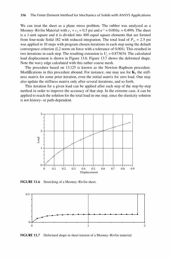
316 The Finite Element Method for Mechanics of Solids with ANSYS Applications
We can treat the sheet as a plane stress problem. The rubber was analyzed as a Mooney–Rivlin Material with c1 = c2 = 0.5 psi and κ–1 = 0.001(ν = 0.499). The sheet is a 1-unit square and it is divided into 400 equal square elements that are formed from four-node Solid 182 with reduced integration. The total load of P11 = 2.5 psi was applied in 10 steps with program chosen iterations in each step using the default convergence criterion (L2 norm on force with a tolerance of 0.001). This resulted in two iterations in each step. The resulting extension is Ux = 0.873634. The calculated load displacement is shown in Figure 13.6. Figure 13.7 shows the deformed shape. Note the wavy edge calculated with this rather coarse mesh.
The procedure based on 13.125 is known as the Newton–Raphson procedure. Modifications in this procedure abound. For instance, one may use for KT the stiff-ness matrix for some prior iteration, even the initial matrix for zero load. One may also update the stiffness matrix only after several iterations, and so forth.
This iteration for a given load can be applied after each step of the step-by-step method in order to improve the accuracy of that step. In the extreme case, it can be applied to reach the solution for the total load in one step, since the elasticity solution is not history- or path-dependent.
0
1
2
3
0 0.1 0.2 0.3 0.4 0.5 0.6 0.7 0.8 0.9
Load
Displacement
fIgure 13.6 Stretching of a Mooney–Rivlin sheet.
0.5
00 1 2
fIgure 13.7 Deformed shape in sheet tension of a Mooney–Rivlin material.
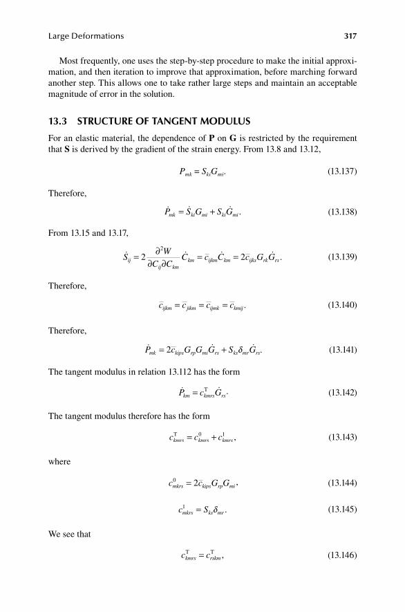
Large Deformations 317
Most frequently, one uses the step-by-step procedure to make the initial approxi-mation, and then iteration to improve that approximation, before marching forward another step. This allows one to take rather large steps and maintain an acceptable magnitude of error in the solution.
13.3 Structure of tangent ModuluS
For an elastic material, the dependence of P on G is restricted by the requirement that S is derived by the gradient of the strain energy. From 13.8 and 13.12,
Pmk = SkiGmi. (13.137)
Therefore,
P S G S Gmk ki mi ki mi= + . (13.138)
From 13.15 and 13.17,
SW
C CC c C c G Gij
ij kmkm ijkm km ijks rk rs= ∂
∂ ∂= =2 2
2
.
(13.139)
Therefore,
c c c cijkm jikm ijmk kmij= = = . (13.140)
Therefore,
P c G G G S Gmk kips rp mi rs ks mr rs= +2 δ . (13.141)
The tangent modulus in relation 13.112 has the form
P c Gkm kmrs rs= T . (13.142)
The tangent modulus therefore has the form
c c ckmrs kmrs kmrsT = +0 1 , (13.143)
where
c c G Gmkrs kips rp mi0 2= , (13.144)
c Smkrs ks mr1 = δ . (13.145)
We see that
c ckmrs rskmT T= , (13.146)

318 The Finite Element Method for Mechanics of Solids with ANSYS Applications
which proves that the tangent modulus is symmetric.Substituting 13.143 into 13.118, one finds that the stiffness matrix has the form
KT = K0 + K1, (13.147)
with an obvious notation. The part K0 of the tangent stiffness matrix is similar to the stiffness of the linear theory but corrected for large displacements. The matrix K1 is the correction for the direction of components of the internal stress in balancing the nodal forces. If the internal stresses are tension, this produces a stress stiffening. If the internal stresses are compressive, this correction can actually add to the effective external loads to produce additional displacements, and if the current stresses are large enough negatively so that
det(K0 + K1) = 0, (13.148)
and buckling occurs. The solution can then be stepped further only when inertial forces are included.
The significance of the terms K0 and K1 is more apparent if the current configura-tion is chosen as the reference configuration for the next step in the calculations. In this case,
Gkm km= δ and G Gkm km0 = . From 13.132, 13.143, and 13.145:
c G G c G G Sijrk im ks mjrs im ks ms jr= +ρρ
ρρ
δ0 0
0 .
(13.149)
By 13.14, the last term depends only on the current stress*:
c G G c Tijrk im ks mjrs ik jr= +ρρ
ρρ
δ0 0
0 .
(13.150)
That is, K1 depends on the current stress.Buckling problems often involve small displacements before buckling occurs. For
small deformations, Gij ≈ δij and ρ ≈ ρ0, and Equation 13.150 reduces to
c c Tijrk ijrk ik jr= + δ , (13.151)
where the first term represents the elasticity coefficients for small strains. This leads to formulation of buckling as an eigenvalue problem.†
13.4 StaBIlIty and BucklIng
In the nonlinear theory, some interesting features can occur that do not occur in the linear theory. In particular, all of the various kinds of buckling phenomena (bifurca-tion or snap-through) may be encountered.
* ANSYS activates the first term by NLGEOM ON and the second term by SSTIFF ON.† ANSYS adds the second term by PRESTRESS ON.
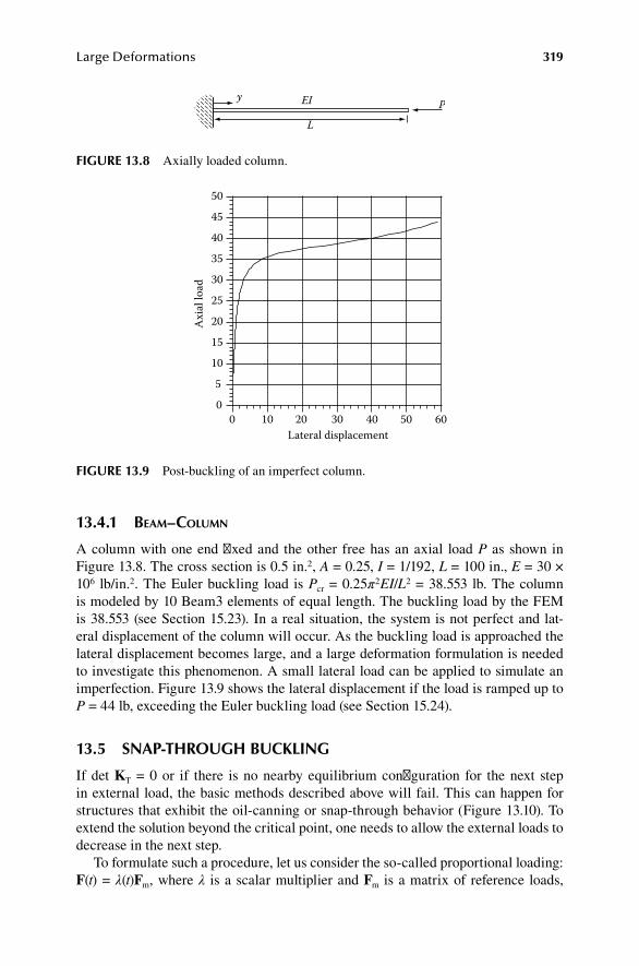
Large Deformations 319
13.4.1 BeaM–coluMn
A column with one end fixed and the other free has an axial load P as shown in Figure 13.8. The cross section is 0.5 in.2, A = 0.25, I = 1/192, L = 100 in., E = 30 × 106 lb/in.2. The Euler buckling load is Pcr = 0.25π2EI/L2 = 38.553 lb. The column is modeled by 10 Beam3 elements of equal length. The buckling load by the FEM is 38.553 (see Section 15.23). In a real situation, the system is not perfect and lat-eral displacement of the column will occur. As the buckling load is approached the lateral displacement becomes large, and a large deformation formulation is needed to investigate this phenomenon. A small lateral load can be applied to simulate an imperfection. Figure 13.9 shows the lateral displacement if the load is ramped up to P = 44 lb, exceeding the Euler buckling load (see Section 15.24).
13.5 Snap-through BucklIng
If det KT = 0 or if there is no nearby equilibrium configuration for the next step in external load, the basic methods described above will fail. This can happen for structures that exhibit the oil-canning or snap-through behavior (Figure 13.10). To extend the solution beyond the critical point, one needs to allow the external loads to decrease in the next step.
To formulate such a procedure, let us consider the so-called proportional loading: F(t) = λ(t)Fm, where λ is a scalar multiplier and Fm is a matrix of reference loads,
L
Py EI
fIgure 13.8 Axially loaded column.
0
5
10
15
20
25
30
35
40
45
50
Lateral displacement20 30 40 50 60100
Axi
al lo
ad
fIgure 13.9 Post-buckling of an imperfect column.

320 The Finite Element Method for Mechanics of Solids with ANSYS Applications
typically the maximum loads to be applied in the analysis. The balance of internal and external node forces becomes
λ(t)Fm = f(t). (13.152)
For a step Δt, we have
F f
F f K D
K
( ) ( ),
( ( ) ) ( ) ( ) ,
( )
t t t t
t t t
t
+ = +
+ = +
∆ ∆
∆ ∆
∆
λ λ m T
T DD F f= + −( ( ) ) ( ).λ λt t∆ m
(13.153)
We now suppose that a solution, λa and Da, has been established for some load-ing, and seek an extension of the solution to a nearby configuration by the iteration scheme
KTΔDi = (λi + Δλi)Fm – f i. (13.154)
The solution of this relation has the form
∆ ∆ ∆Di i i= +λ D Dm , (13.155)
where
KTDm = Fm, (13.156)
K D F fT m∆ i i i= −λ . (13.157)
–20
–10
0
10
20
30
40
50
60
70
80
0 0.5 1 1.5 2 2.5
Forc
e
Displacement
fIgure 13.10 Snap-through buckling.

Large Deformations 321
We need a method for determination of Δλi. The arc length method8–10 can be used.
A step change in D and λ has length s given by (using nondimensional variables)
s D Di
Ki
Ka
K
2 2 2= − + −∑( ) ( )λ λa . (13.158)
This is illustrated in Figure 13.11 for a single degree of freedom system. We choose the first step so that s is small and hold s constant for subsequent itera-tions. This allows the load parameter λ to decrease if necessary while the magni-tude of displacement increases. The derivative of 13.158 provides the constraint relation:
( ) ( ) .λ λ λi i
Ki
Ka
Ki
K
D D D− + − =∑a ∆ ∆ 0 (13.159)
Using 13.155, we find
∆∆
λλ λ
iKi
Ka
Ki
K
iKi
Ka
Km
K
D D D
D D D=
− −
− + −
∑∑( )
( )a
. (13.160)
The increment in displacement can now be calculated from 13.155. The tangent stiff-ness can be unchanged in each iteration or updated as corrections are made to the updated reference configuration.
The finite steps calculated by 13.159 will result in small increases in arc length s defined by 13.158 as shown in Figure 13.11. For a single degree of freedom, let
ti = (Di – Da)e1 + (λi – λa)e2, (13.161)
ni = ΔDie1 + Δλie2. (13.162)
Da Di
λa
λi∆Di
∆λi
s
fIgure 13.11 Arc length method.

322 The Finite Element Method for Mechanics of Solids with ANSYS Applications
The condition ∣ti∣ = s and condition 13.159 are equivalent to the condition ti ∙ ni = 0, that ti and ni are orthogonal. Each iteration to ti+1 = ti + ni will therefore increase the arc length slightly to a = ∣ti+1∣:
a2 = s2 + (Δλi)2 + (ΔDi)2. (13.163)
A simple correction can be made to preserve the arc length.11 The vector
r ti ia s
a= − − +1
(13.164)
is the correction needed to preserve the arc length. From the geometry of the right triangle in Figure 13.11, we find
t r t ti i i ia s
aa s s
a⋅ = − − ⋅ = − −+1
2( ). (13.165)
The corrected step mi = ni + ri is not orthogonal to ti. Let
R
a s sa
i i i i i= ⋅ = ⋅ = − −t m t r
( ) 2
. (13.166)
The corrected increments Δλi and ΔDi are given by
mi = ΔDie1 + Δλie2. (13.167)
Using 13.155 and inserting into 13.166, we find the formula for the corrected load step:
∆
∆λ
λ λi
i ia
i
i ia m
R D D D
D D D= − −
− + −( )
( ).
a
(13.168)
The modified procedure for multiple degrees of freedom is as follows:
1. ∆∆
λλ λ
iKi
Ka
Ki
K
iKi
Ka
Km
K
D D D
D D D=
− −
− + −
∑∑( )
( )a
(causes growth in arc length)
2. ∆ ∆ ∆D D Di im
i= +λ
3. a s Di i2 2 22
= + +( )∆ ∆λ (increased arc length)
4. Ra s s
ai = − −( ) 2
(correction factor)
5. ∆∆
λλ λ
i
iKi
Ka
Ki
K
iKi
Ka
Km
K
R D D D
D D D=
− −
− + −
∑∑
( )
( )a
(correction to load factor)
6. ∆ ∆ ∆Di im
i= +λ D D (using corrected load factor)
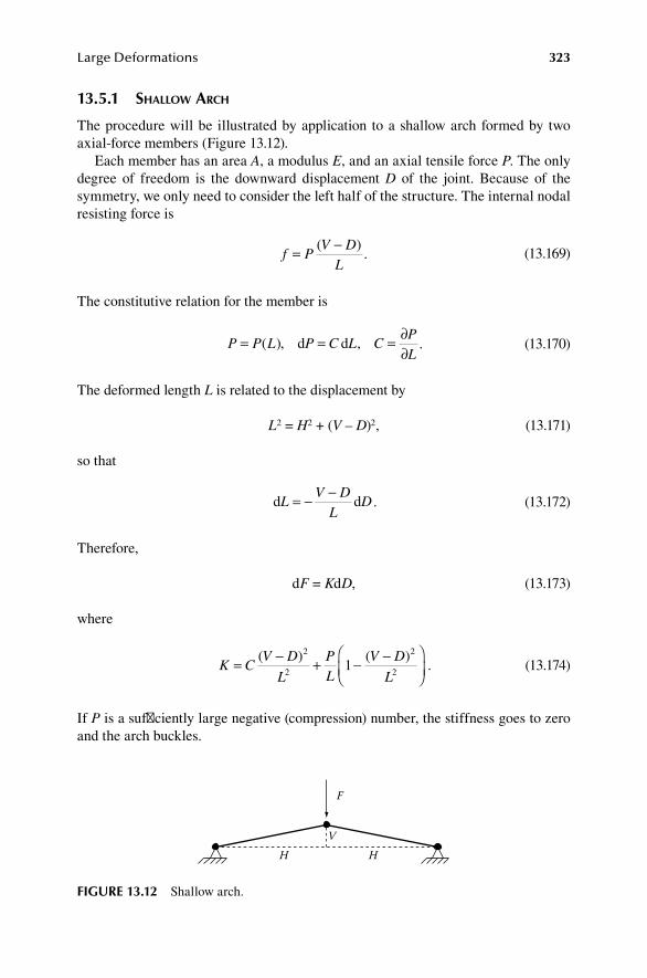
Large Deformations 323
13.5.1 Shallow arch
The procedure will be illustrated by application to a shallow arch formed by two axial-force members (Figure 13.12).
Each member has an area A, a modulus E, and an axial tensile force P. The only degree of freedom is the downward displacement D of the joint. Because of the symmetry, we only need to consider the left half of the structure. The internal nodal resisting force is
f P
V DL
= −( ).
(13.169)
The constitutive relation for the member is
P P L P C L C
PL
= = = ∂∂
( ), ,d d . (13.170)
The deformed length L is related to the displacement by
L2 = H2 + (V – D)2, (13.171)
so that
d dL
V DL
D= − −. (13.172)
Therefore,
dF = KdD, (13.173)
where
K C
V D
L
PL
V D
L= − + − −
( ) ( )2
2
2
21 . (13.174)
If P is a sufficiently large negative (compression) number, the stiffness goes to zero and the arch buckles.
F
VHH
fIgure 13.12 Shallow arch.
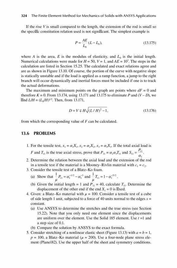
324 The Finite Element Method for Mechanics of Solids with ANSYS Applications
If the rise V is small compared to the length, the extension of the rod is small so the specific constitution relation used is not significant. The simplest example is
P
AEL
L L= −0
0( ),
(13.175)
where A is the area, E is the modulus of elasticity, and L0 is the initial length. Numerical calculations were made for H = 50, V = 1, and AE = 107. The steps in the calculation are listed in Section 15.25. The calculated and exact relations agree and are as shown in Figure 13.10. Of course, the portion of the curve with negative slope is statically unstable and if the load is applied as a ramp function, a jump to the right branch will occur dynamically and inertial forces must be included if one is to track the actual deformations.
The maximum and minimum points on the graph are points where dF = 0 and therefore K = 0. From 13.174, using 13.171 and 13.175 to eliminate P and (V – D), we find L/H = (L0/H)1/3. Then, from 13.171,
D V H L H= − ( / ) ,2 1 (13.176)
from which the corresponding value of F can be calculated.
13.6 proBleMS
1. For the tensile test, x1 = α1X1, x2 = α2X2, x3 = α3X3. If the total axial load is
F and T11 is the true axial stress, prove that P11 = α2α3T11 and SP
1111
1
=α
.
2. Determine the relation between the axial load and the extension of the rod in a tensile test if the material is a Mooney–Rivlin material with c1 = c2.
3. Consider the tensile test of a Blatz–Ko foam.
(a) Show that 1
11 11 2
13
µα αP = −− −/ and
1111 1
5 2
µαT = − − / .
(b) Given the initial length = 1 and P11 = 40, calculate T11. Determine the displacement of the other end if the end X1 = 0 is fixed.
4. Given: a Blatz–Ko material with μ = 100. Consider a tensile test of a cube of side length 1 unit, subjected to a force of 40 units normal to the edges x = constant.(a) Use ANSYS to determine the stretches and the true stress (see Section
15.22). Note that you only need one element since the displacements are uniform over the element. Use the Solid 185 element. Use t =1 and a step size of 0.1.
(b) Compare the solution by ANSYS to the exact formula. 5. Consider stretching of a nonlinear elastic sheet (Figure 13.13) with a = b = 1,
p = 100, a Blatz–Ko material (μ = 200). Use a four-node plane stress ele-ment (Plane182). Use the upper half of the sheet and symmetry conditions.
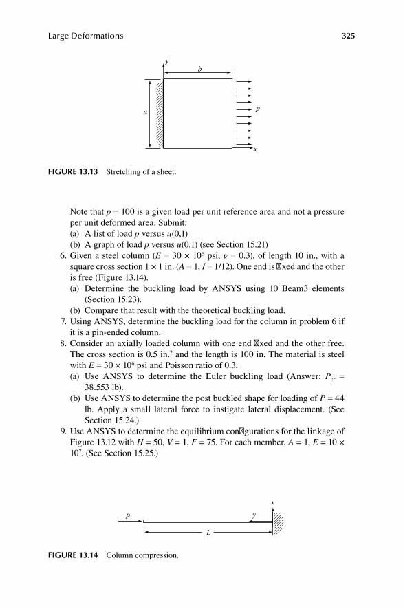
Large Deformations 325
Note that p = 100 is a given load per unit reference area and not a pressure per unit deformed area. Submit:(a) A list of load p versus u(0,1)(b) A graph of load p versus u(0,1) (see Section 15.21)
6. Given a steel column (E = 30 × 106 psi, ν = 0.3), of length 10 in., with a square cross section 1 × 1 in. (A = 1, I = 1/12). One end is fixed and the other is free (Figure 13.14).(a) Determine the buckling load by ANSYS using 10 Beam3 elements
(Section 15.23).(b) Compare that result with the theoretical buckling load.
7. Using ANSYS, determine the buckling load for the column in problem 6 if it is a pin-ended column.
8. Consider an axially loaded column with one end fixed and the other free. The cross section is 0.5 in.2 and the length is 100 in. The material is steel with E = 30 × 106 psi and Poisson ratio of 0.3.(a) Use ANSYS to determine the Euler buckling load (Answer: Pcr =
38.553 lb).(b) Use ANSYS to determine the post buckled shape for loading of P = 44
lb. Apply a small lateral force to instigate lateral displacement. (See Section 15.24.)
9. Use ANSYS to determine the equilibrium configurations for the linkage of Figure 13.12 with H = 50, V = 1, F = 75. For each member, A = 1, E = 10 × 107. (See Section 15.25.)
p
x
by
a
fIgure 13.13 Stretching of a sheet.
L
P y
x
fIgure 13.14 Column compression.

326 The Finite Element Method for Mechanics of Solids with ANSYS Applications
referenceS
1. Ogden, R. W., Non-linear Elastic Deformations, 219, Dover Publications, New York, 1997.
2. Simo, J. C., and T. J. R. Hughes, Computational Inelasticity, Springer-Verlag, New York, 1998.
3. Mooney, M., A theory of large elastic deformation, J. Appl. Phys., 6, 582–592, 1940. 4. Rivlin, R. S., Forty years of nonlinear continuum mechanics, Proceedings of the IX
International Congress on Rheology, Mexico, pp. 1–29, 1984. 5. Blatz, P. J., and W. L. Ko, Application of finite elastic theory to the deformation of rub-
bery materials, Trans. Soc. Rheol., 6, 223–251, 1962. 6. Kao, B. G., and L. Razgunas, On the determination of strain energy functions of rub-
bers, Proceedings of the VI International Conference on Vehicle Structural Mechanics, Detroit, MI, pp. 145–154, 1986.
7. Yeoh, O. H., Characterization of elastic properties of carbon-black-filled rubber vulca-nizates, Rubber Chem. Technol., 63, 792, 1990.
8. Wempner, G. A., Discrete approximations related to nonlinear theories of solids, Int. J. Solids Struct., 7, 1581–1599, 1971.
9. Riks, E., The application of Newton’s method to the problem of elastic stability, J. Appl. Mech., 39, 1581–1599, 1972.
10. E. Riks, An incremental approach to the solution of snapping and buckling problems, Int. J. Solids Struct., 15, 529–551, 1979.
11. Forde, B. W. R., and S. F. Stiemer, Improved arc length orthogonality methods for non-linear finite element analysis, Comput. Struct., 27, 625–630, 1987.
BIBlIography
Bathe, K. J., Finite Element Procedures, Prentice-Hall, Englewood Cliffs, NJ, 1996.Dill, E. H., Continuum Mechanics: Elasticity, Plasticity, Viscoelasticity, CRC Press, Boca
Raton, FL, 2007.Holzapfel, G. A., Nonlinear Solid Mechanics, Wiley, New York, 2000.Ogden, R. W., Non-Linear Elastic Deformations, Dover Pub., Mineola, NY, 1997.

327
14 Constraints and Contact
14.1 applIcatIon of conStraIntS
We often encounter situations in which the degrees of freedom D are not indepen-dent or they are limited in range. This is often expressible as a constraint of the form of n linear equations:
CD – Q = 0, (14.1)
where matrices C and Q are constant. For example, consider the axially loaded rod in which one element is modeled as a rigid body (Figure 14.1). This condition can be applied as a constraint on the nodal displacements:
u1 – u2 = 0. (14.2)
The constraints could be applied directly to the assembled finite element equations to reduce the number of independent variables. However, it is more convenient to incorporate the constraints 14.1 indirectly in order to provide for the general situa-tion. There are two commonly used methods to do this: Lagrange multipliers and the penalty method.
14.1.1 lagrange MultiplierS
In the Lagrange multiplier method, the potential energy of the unconstrained struc-ture with a nonrigid element is modified to include the constraints. For constraints of the form 14.1, set
d = CD – Q. (14.3)
The potential energy of the unconstrained structure is
Π0
12
= −D KD D FT T .
(14.4)
This includes the members that are to be constrained. That is, member 1–2 in Figure 14.1 is to be included as an elastic element.
The potential energy is augmented by
Πc = λTd. (14.5)
The matrix λ is a diagonal matrix of parameters λi, which are additional independent variables called Lagrange multipliers.
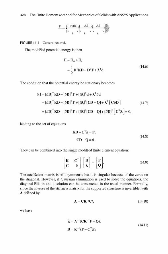
328 The Finite Element Method for Mechanics of Solids with ANSYS Applications
The modified potential energy is then
Π Π Π= +
= − +
0
12
c
T T TD KD D F dλλ .
(14.6)
The condition that the potential energy be stationary becomes
δ δ δ δ δ
δ δ δ
Π = − + +
= − +
[ ] [ ] [
[ ] [ ] [
D KD D F d d
D KD D F
T T T T
T T
λλ]] λλ
λλλλ]] λλ
λλ]]
T T
T T T
[ ]
[ ] [ ] [ [ ]
CD Q C D
D KD D F CD Q
− +
= − + −
δ
δ δ δ ++ =[ ] ,δ D CT Tλλ 0
(14.7)
leading to the set of equations
KD C F
CD Q 0
+
− =
Tλλ == ,
.
(14.8)
They can be combined into the single modified finite element equation:
K CC 0
D FQ
T
=
λλ.
(14.9)
The coefficient matrix is still symmetric but it is singular because of the zeros on the diagonal. However, if Gaussian elimination is used to solve the equations, the diagonal fills in and a solution can be constructed in the usual manner. Formally, since the inverse of the stiffness matrix for the supported structure is invertible, with A defined by
A = CK–1CT, (14.10)
we have
λλ
λλ))
= −
= −
− −
−
A CK F Q
D K F C
1 1
1
( ),
( T .
(14.11)
P 1 rigid 2 AE AE3
L L L
fIgure 14.1 Constrained rod.

Constraints and Contact 329
In the example shown in Figure 14.1, ignoring the constraints, and assigning the same AE to element 1–2,
K D=−
− −−
=
k kk k k
k k
u
u
u
02
0 2
1
2
3
,
=
, .FP00
(14.12)
The rigid constraint of member 1–2 is expressed by
C Q 0= − =1 1 0 , . (14.13)
The modified finite element equations 14.8 are therefore
k kk k k
k k
u
u
u
−− − −
−−
0 12 1
0 2 01 1 0 0
1
2
3
λ
=
P000
.
(14.14)
The solution by Gaussian elimination is
λ
λ
=
=
= + =
= − + =
P
uPk
uPk
uPk
uPk k
u u
,
,
,
.
3
2 3
1 2 2
2
(14.15)
Note that the Lagrange multiplier can be interpreted as the reactive force due to the imposed constraint. This is also evident from the potential energy expression 14.6, where the term λTd can be regarded as the potential for the “forces” λ, or from the virtual work expression 14.7 by the term λTδd.
14.1.2 perturBed lagrangian Method
The zero diagonal element in the Lagrange multiplier method can be removed by the perturbed Lagrangian method. In this method, the potential (14.5) for the constraint is altered as follows.

330 The Finite Element Method for Mechanics of Solids with ANSYS Applications
Πc
T T= +λλ λλ λλd12κ
.
(14.16)
Then,
δ δ δ δ δΠ == − + − + −[ ] [ ] [ [ ] [ ] [D KD F CD Q D CT T T Tλλ]] λλ λλ]]1
κTT λλ.
(14.17)
For the example shown in Figure 14.1, when the last term is merged into 14.14 we have
k kk k k
k k
u
u
u
−− − −
−
−
0 12 1
0 2 0
1 1 01
1
2
3
κ λλ
=
P000
.
(14.18)
The last equation can now be used to eliminate the Lagrange multiplier,
λ = κ(u2 – u1), (14.19)
and the remaining equations are
k kk k k
k k
u
u
u
− − +− + − −
−
κ κκ κ
02
0 2
1
2
3
=
P00
.
(14.20)
The solution is
uPk
u u u u
k
k3 2 3 1 221
32
1= = =
−
−, , .κ
κ
(14.21)
For infinite κ, the exact result is obtained. For κ = k × (10)3, we obtain an approximate solution:
u1 = 0.9994995 u2 (14.22)
The zero on the diagonal has been removed, but the solution is now only approximate.

Constraints and Contact 331
14.1.3 penalty functionS
In this method, the addition to the potential energy is
Πp
T= 12
d dαα ,
(14.23)
where α is a diagonal matrix of constants αi called penalty numbers. The modified potential energy is
Π = − +1
212
D KD D F d dT T Tαα .
(14.24)
The condition that the potential energy is stationary becomes
δ δ δ δ
δ δ δ
Π = − +
= − +
[ ] [ ] [ ]
[ ] [ ] [ ]
D KD D F d d
D KD D F C D
T T T
T T T
αα
αααα
αα −− −− αα ]] == 00
[ ]
[ ] [
CD Q
D KD C CD F C Q
−
= +δ T T T .
(14.25)
Therefore,
[K + CT αC]D = [F + CT αQ]. (14.26)
The solution of this equation for very large α provides an approximate solution to the constrained finite element equations.
For the example presented in Figure 14.1, we have
C CTαα == α α110
1 1 01 1 01 1 00 0 0
−
− =−
−
.
(14.27)
The penalized equations 14.26 become
k kk k k
k k
u
u
u
+ − −− − + −
−
α αα α
02
0 2
1
2
3
=
P00
.
(14.28)
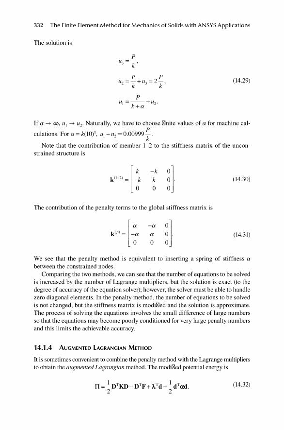
332 The Finite Element Method for Mechanics of Solids with ANSYS Applications
The solution is
uPk
uPk
uPk
uP
ku
3
2 3
1 2
2
=
= + =
=+
+
,
,
.α
(14.29)
If α → ∞, u1 → u2. Naturally, we have to choose finite values of α for machine cal-
culations. For α = k(10)3, u uPk1 2 0 00999− = . .
Note that the contribution of member 1–2 to the stiffness matrix of the uncon-strained structure is
k( )1 2
00
0 0 0
− =−
−
k kk k .
(14.30)
The contribution of the penalty terms to the global stiffness matrix is
k( ) .p =−
−
α αα α
00
0 0 0
(14.31)
We see that the penalty method is equivalent to inserting a spring of stiffness α between the constrained nodes.
Comparing the two methods, we can see that the number of equations to be solved is increased by the number of Lagrange multipliers, but the solution is exact (to the degree of accuracy of the equation solver); however, the solver must be able to handle zero diagonal elements. In the penalty method, the number of equations to be solved is not changed, but the stiffness matrix is modified and the solution is approximate. The process of solving the equations involves the small difference of large numbers so that the equations may become poorly conditioned for very large penalty numbers and this limits the achievable accuracy.
14.1.4 augMented lagrangian Method
It is sometimes convenient to combine the penalty method with the Lagrange multipliers to obtain the augmented Lagrangian method. The modified potential energy is
Π = − + +1
212
D KD D F d d dT T T Tλλ αα .
(14.32)

Constraints and Contact 333
Combining 14.14 and 14.28, we obtain the following equations for the example (Figure 14.1):
k kk k k
k k
u
u+ − −
− − + − −−−
α αα α
0 12 1
0 2 01 1 0 0
1
22
3
000
u
P
λ
=
.
(14.33)
The solution is
λ = = = =P u u u
Pk
, .1 2 32 2
(14.34)
In this example, there is no advantage. The penalty number α drops out and the exact solution is obtained.
14.2 contact proBleMS
Problems involving the contact between two bodies, such as an automobile tire upon the pavement or the bearing of a bolt against the bolt hole, are far more complicated than the single body problems so far considered. The actual contact surface is usually not known in advance, and the boundary conditions on this unknown surface involve tractions and displacements that are not known in advance. Consequently, the contact problem is gov-erned by a system of inequalities and one must proceed in a step-by-step or an iterative manner. The formulation will again make use of the Lagrange multiplier method and the penalty method. In this chapter, we will only introduce the basic concepts of the analysis. ANSYS provides the option of a pure penalty method, a pure Lagrangian method, the augmented Lagrangian method, or the Lagrangian multiplier on the contact normal and the penalty factor on the frictional direction.
14.2.1 exaMple: a truSS contactS a rigid foundation
This class of problems is illustrated by the deformation of the truss (Figure 14.2) that comes into contact with a rigid foundation when the load is large enough.
The constraint condition is
g – V ≥ 0. (14.35)
We will analyze the case when the member stiffness AE/L is 25 for member 1 and 50 for member 2. The finite element equation for the supported structure is
K UV
F
Fx
y
=
(14.36)

334 The Finite Element Method for Mechanics of Solids with ANSYS Applications
with
K = −−
27 1212 48
.
(14.37)
Before contact with the rigid foundation,
UF F
VF F
x y
x y
= +
= +
24 96
96
3
128
,
.
(14.38)
Figure 14.3 shows the nodal forces before contact. After contact at U = Uc and V = g, with increasing loads, the node may stick or it may slide on the foundation. The foun-dation provides a force p resisting penetration and a force f resisting sliding (Figure 14.4). The equilibrium equations are
F f U g
F p U g
x
y
− = −
− = − +
27 12
12 48
,
.
(14.39)
3L 3L
4L12
x
y
Fy ,VFx ,U
g
fIgure 14.2 Truss and foundation.
27U – 12V
–12U + 48V
Fy
Fx
fIgure 14.3 Equilibrium before contact.

Constraints and Contact 335
For the stick condition, U = Uc so that p and f are determined by the equilibrium equations for given loads that are large enough to maintain contact. The load and displacement at contact depends on the load path. We will consider two examples.
14.2.1.1 load Fy > 0 Is applied with Fx = 0Contact (V = g) occurs for
F
gFy = ≡128
3 c
(14.40)
at
U g U= ≡4
9 c.
(14.41)
If Fx = 0 after contact, any additional load in the y direction is transmitted directly to the foundation without deformation of the structure. Figure 14.5 shows the nodal forces in this case: Fy > Fc and Fx = 0. The foundation exerts a reaction force p = Fy – Fc and f = 0. If Fy = Fc after contact, a load in the x direction cannot increase the V displacement. The structure may stick to the target (no additional U displace-ment); or, if Fx is large enough, it may slip along the support (U > 0). The foundation may resist the slip (U displacement) by friction between the structure and the rigid foundation, and then a formula for f is required. We will only consider the so-called Coulomb friction: f = μp. Figure 14.6 shows the nodal forces for Fy = Fc and Fx > 0 for slip with no friction. The nodal forces for slip including a friction force f = μp are shown in Figure 14.7. In this case, Fx = (27 + 12μ)(U – Uc).
27U – 12g
–12U + 48g
f pFy
Fx
fIgure 14.4 Equilibrium after contact.
1283
3
g
g128p = Fy –Fy
fIgure 14.5 After contact Fy > Fc.

336 The Finite Element Method for Mechanics of Solids with ANSYS Applications
14.2.1.2 loads are ramped up together: Fx = 27α, Fy = 12.8αContact occurs for
α =
=
=
=
1 7204
46 4516
22 0215
2 1649
. ,
. ,
. ,
. .
g
F g
F g
U g
x
y
(14.42)
After contact, the node may stick without further deformation and additional loads are reacted by the foundation. Or the node may slip along the foundation. If the loads are increased in the same ratio with no resistance to slip ( f = 0), the equilibrium equations 14.39 give
UF g
p F U g
x
y
= +
= + −
1227
12 48
,
.
(14.43)
If there is a resistance to slip for which f = μp, the equilibrium equations 14.39 yield
UF F g
p F U g
x y
y
=− + +
+
= + −
µ µµ
( ),
.
12 48
27 12
12 48
(14.44)
We will now formulate the problem using Lagrange multipliers and penalty func-tions to impose the constraint.
–12U + 48g
27U – 12g
p = 12(U – Uc) = 49
Fx
Fc Fx
fIgure 14.6 Slip without friction.
–12U + 48g
27U – 12g
p = 12(U – Uc)
Fx
Fc
pf = µ
fIgure 14.7 Slip with friction force.

Constraints and Contact 337
14.2.2 lagrange Multiplier, no friction force
After contact, the constraint on the normal displacement is
gn = g – V = 0 (14.45)
and the addition to the potential energy of the unconstrained structure is
Πc = λngn = λ(g – V). (14.46)
The first variation provides the additions to the virtual work:
δΠc = δλ(g – V) + λ(–δV). (14.47)
The modified finite element relation 14.36 is therefore
27 12 012 48 10 1 0
−− −
−
=
−
UV
F
F
g
x
y
λ
.
(14.48)
The equations are to be solved subject to the condition
λ(g – V) = 0. (14.49)
That is, for g – V < 0 we have λ = 0, and for g – V = 0 we have to find λ by solving the matrix equation. Before contact, given Fx = 0 and Fy > 0, the solution is
λ = = =0
96
3
128, , ,U
FV
Fy y
(14.50)
as in 14.38. At initial contact,
λ = = = = =0
49
1283
, , , ,V g U g F g Fy c
(14.51)
as in 14.40 and 14.41. If the loads are ramped up, Fx = 27α, Fy = 12.8α, after contact V = g and we have
UF g
F U g
x
y
= +
= + −
1227
12 48
,
.λ
(14.52)

338 The Finite Element Method for Mechanics of Solids with ANSYS Applications
This agrees exactly with 14.43 and shows λ = p. Initial contact occurs at λ = 0, which leads to the result 14.42. The solution for this case is set forth in Section 15.32.
14.2.2.1 Stick conditionGiven Fx = 0 and Fy > Fc, the solution is
U g
V g
F gy
=
=
= − −
<
49
1283
0
,
,
.λ
(14.53)
Comparing this result with Figure 14.5, we identify the Lagrange multiplier as the reaction force of the foundation on the structure: λ = –p.
14.2.2.2 Slip condition
Given Fx > 0 and F gy = 1283
, the solution is
V g
UF
g
U g F
x
x
=
= +
= − −
= −
,
,
,
2749
1249
1227
λ
(14.54)
as shown in Figure 14.6. The Lagrange multiplier provides the reaction force pre-venting penetration of the support during slip: λ = –p.
14.2.3 lagrange Multiplier, with friction
The amount of slip is
g U U U gt c c= − =, .
49
(14.55)
The addition to the potential energy is
Πc = λngn + λtgt (14.56)
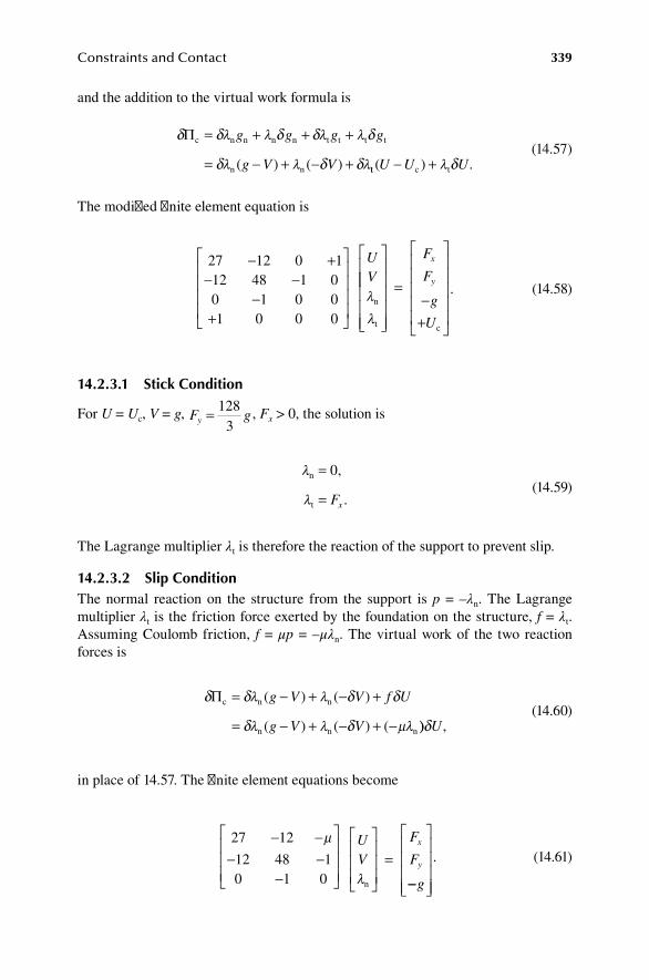
Constraints and Contact 339
and the addition to the virtual work formula is
δ δ δ δ δ
δ δ δ
Πc n n n n t t t t
n n
= + + +
= − + − +
λ λ λ λ
λ λ λ
g g g g
g V V( ) ( ) tt c t( ) .U U U− + λ δ
(14.57)
The modified finite element equation is
27 12 0 112 48 1 00 1 0 01 0 0 0
− +− −
−+
UVλ
λn
t
=−
+
F
F
g
U
x
y
c
.
(14.58)
14.2.3.1 Stick condition
For U = Uc, V = g, F gy = 1283
, Fx > 0, the solution is
λ
λ
n
t
=
=
0,
.Fx (14.59)
The Lagrange multiplier λt is therefore the reaction of the support to prevent slip.
14.2.3.2 Slip conditionThe normal reaction on the structure from the support is p = –λn. The Lagrange multiplier λt is the friction force exerted by the foundation on the structure, f = λt. Assuming Coulomb friction, f = μp = –μλn. The virtual work of the two reaction forces is
δ δ δ δ
δ δ
Πc n n
n n n
= − + − +
= − + − + −
λ λ
λ λ µλ
( ) ( )
( ) ( ) (
g V V f U
g V V )) ,δU
(14.60)
in place of 14.57. The finite element equations become
27 12
12 48 10 1 0
− −− −
−
=µ
λ
UV
F
Fx
y
n −−
g
.
(14.61)
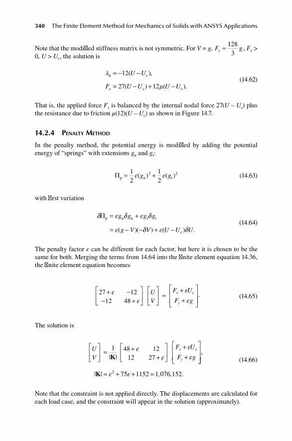
340 The Finite Element Method for Mechanics of Solids with ANSYS Applications
Note that the modified stiffness matrix is not symmetric. For V = g, F gy = 1283
, Fx > 0, U > Uc, the solution is
λ
µ
n c
c c
= − −
= − + −
12
27 12
( ),
( ) ( ).
U U
F U U U Ux
(14.62)
That is, the applied force Fx is balanced by the internal nodal force 27(U – Uc) plus the resistance due to friction μ(12)(U – Uc) as shown in Figure 14.7.
14.2.4 penalty Method
In the penalty method, the potential energy is modified by adding the potential energy of “springs” with extensions gn and gt:
Πp n t= +1
212
2 2ε ε( ) ( )g g
(14.63)
with first variation
δ δ δ
δ δ
Πp n n t t
c
= +
= − − + −
ε ε
ε ε
g g g g
g V V U U U( )( ) ( ) .
(14.64)
The penalty factor ε can be different for each factor, but here it is chosen to be the same for both. Merging the terms from 14.64 into the finite element equation 14.36, the finite element equation becomes
27 1212 48+ −
− +
=
++
ε
ε
ε
εUV
F U
F gx
y
c
.
(14.65)
The solution is
UV
F U
F gx
y
= +
+
++
1 48 1212 27| |
c
Kε
ε
ε
ε
= + + =
,
, , .| |K ε ε2 75 1152 1 076 152
(14.66)
Note that the constraint is not applied directly. The displacements are calculated for each load case, and the constraint will appear in the solution (approximately).

Constraints and Contact 341
14.2.4.1 Stick conditionFor the load case Fx = 0 and Fy > Fc, choosing ε = 1000, the solution is
V g F F
U U F F
y
y
= + −
= + −
0 0009543
0 00001115
. ( ),
. ( ).
c
c c
(14.67)
Naturally, because of round-off error the first terms will not be returned exactly by the computer. We see that constraint V = g and contact point U = Uc are only approxi-mated. There is some penetration of the target, as shown by the second term. The value of ε is arbitrary but must be large enough so that the penetration is negligible.
14.2.4.2 Slip conditionIf there is a resistance to slip due to Coulomb friction, the virtual work expression 14.64 must be altered to express the work of the friction force f = μp = –μεgn:
δ δ δ
δ δ
Πp n n t= +
= − − − −
ε
ε µε
g g f g
g V V g V U( )( ) ( ) .
(14.68)
Merging with the equation for the unconstrained structure, we have
27 12
12 48
− +− +
=
++
µεε
µε
εUV
F g
F gx
y
. (14.69)
Note that the modified stiffness is not symmetric because of the friction force. The solution for ε = (10)4 and μ = 0.5 is
V g U U F F
F Fx
= + − + −
−
0 001194 0 0000995
0 9928
. ( ) . ( ),
. (
c c
µ −− = − + −F U U U Uc c c) ( ) . ( ).27 11 914µ
(14.70)
The exact solution from 14.38 is
V g
F F F U U U Ux
=
− − = − + −
,
( ) ( ) ( )µ µc c c27 12 . (14.71)
14.3 fInIte eleMent analySIS
The contact problem is complicated because the topology of the system changes upon contact. The equilibrium equations before contact, for example, 14.38, are the stan-dard finite element equations. The equilibrium equations after contact, for example,

342 The Finite Element Method for Mechanics of Solids with ANSYS Applications
14.39, are completely different and contain new unknowns. One must specify “stick” or “slip” conditions and a constitutive relation for the slip reaction f.
The solution procedure is necessarily incremental. After each load step, one must determine whether the bodies are in contact. A procedure must be devised to calcu-late the gap from information available in the finite element analysis. In the general case of two- or three-dimensional bodies, multiple nodes can come into contact with the finite elements forming the boundary of the target. Furthermore, after contact a node may continue in contact or it may move away, thereby creating a new gap. Because each load step is finite, initial contact occurs as a penetration of one body into another. Iteration is the necessary factor within the load step to reduce the pen-etration to an allowable magnitude. ANSYS treats the problem of calculating the contact of surfaces by overlaying on the given bodies, a pair of contact surfaces that interact with each other to prevent penetration and to allow calculation of the required pressures. One surface is regarded as the target and the other as the contact-ing surface. The contact pair must cover the potential contact region.
14.3.1 exaMple: contact of a cylinder with a rigid plane
Let us consider a long elastic cylinder compressed between two rigid clamps (Figure 14.8). The body is analyzed as a plane strain, which will apply to a long cylinder except near the ends.
The solution to this problem is known.1 The half-contact width b is given by
b
FR2 2 1
( ).
− νπµ
(14.72)
The contact pressure is
p
Fb
x b= −21 2
π( ) ./
(14.73)
The displacement of a rigid clamp is
dF= −
−
( )
.1 4 1
2ν
πµln
Rb
(14.74)
2R–2d
F
F
2bR
yx
fIgure 14.8 Compressed cylinder.
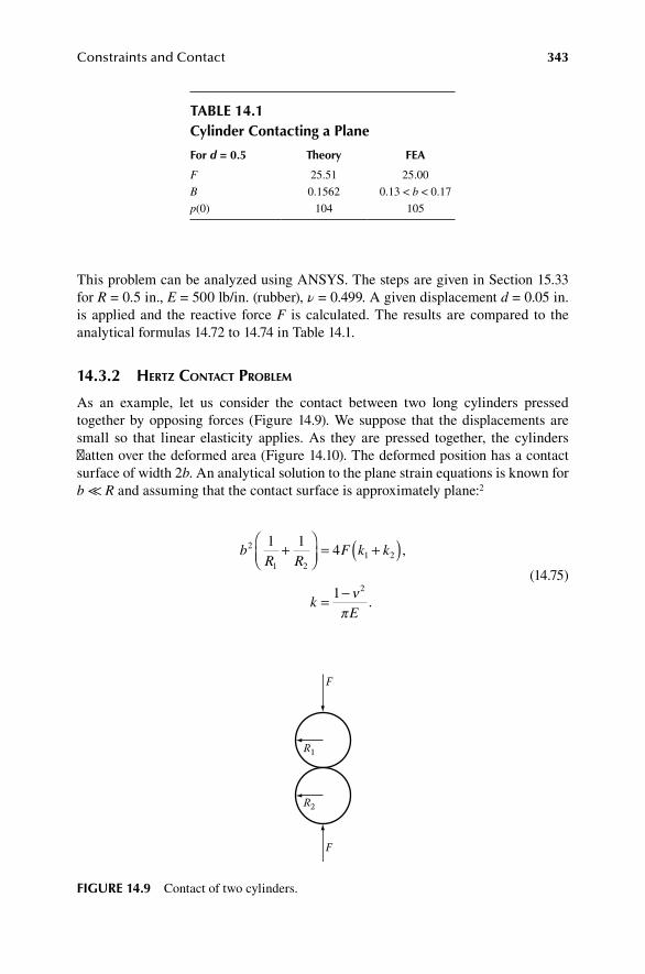
Constraints and Contact 343
This problem can be analyzed using ANSYS. The steps are given in Section 15.33 for R = 0.5 in., E = 500 lb/in. (rubber), ν = 0.499. A given displacement d = 0.05 in. is applied and the reactive force F is calculated. The results are compared to the analytical formulas 14.72 to 14.74 in Table 14.1.
14.3.2 hertz contact proBleM
As an example, let us consider the contact between two long cylinders pressed together by opposing forces (Figure 14.9). We suppose that the displacements are small so that linear elasticity applies. As they are pressed together, the cylinders flatten over the deformed area (Figure 14.10). The deformed position has a contact surface of width 2b. An analytical solution to the plane strain equations is known for b ≪ R and assuming that the contact surface is approximately plane:2
bR R
F k k
kE
2
1 21 2
2
1 14
1
+
= +( )
= −
,
.ν
π
(14.75)
taBle 14.1cylinder contacting a plane
for d = 0.5 theory fea
F 25.51 25.00
B 0.1562 0.13 < b < 0.17
p(0) 104 105
F
F
R1
R2
fIgure 14.9 Contact of two cylinders.
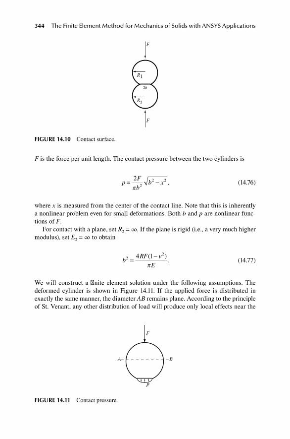
344 The Finite Element Method for Mechanics of Solids with ANSYS Applications
F is the force per unit length. The contact pressure between the two cylinders is
p
F
bb x= −2
22 2
π,
(14.76)
where x is measured from the center of the contact line. Note that this is inherently a nonlinear problem even for small deformations. Both b and p are nonlinear func-tions of F.
For contact with a plane, set R2 = ∞. If the plane is rigid (i.e., a very much higher modulus), set E2 = ∞ to obtain
b
RFE
224 1= −( )ν
π.
(14.77)
We will construct a finite element solution under the following assumptions. The deformed cylinder is shown in Figure 14.11. If the applied force is distributed in exactly the same manner, the diameter AB remains plane. According to the principle of St. Venant, any other distribution of load will produce only local effects near the
F
F
R1
R2
2b
fIgure 14.10 Contact surface.
A B
F
p
fIgure 14.11 Contact pressure.

Constraints and Contact 345
load. We will therefore assume that AB remains straight. We will then have double symmetry and can restrict the analysis to one-quarter of each sphere as shown in Figure 14.12. It is also easier to specify a displacement of line AB rather than force F. The magnitude of the force is then a reaction. If the displacement is not specified, there is no initial constraint on translation in the y direction. Consequently, the initial stiffness matrix for each cylinder has zero determinant because of the possible rigid body motion.
If the force is to be specified instead of the displacement, the analysis can proceed in two steps: (1) apply a very small displacement to create contact and (2) apply load F to the assembly.
ANSYS treats the problem of calculating the contact of surfaces by overlaying on the given bodies a pair of contact surfaces that interact with each other to prevent penetration and allow calculation of the required pressures. One surface is regarded as the target and the other as the contacting surface. The contact pair must cover the potential contact region (Figure 14.13).
ux = 0
uy = 0
uy = d
x
y
fIgure14.12 Reduction by symmetry.
contact surface
target surface
uy = 0
ux = 0
uy = d
x
ν2
ν1
α2
α1
R2
R1
E2
E1
y
fIgure 14.13 Contact pair model.

346 The Finite Element Method for Mechanics of Solids with ANSYS Applications
A possible calculation is given in Section 15.34 for R1 = 10 mm, R2 = 13 mm, E1 = E2 = 30,000 N/mm2, ν1 = ν2 = 0.25. The calculated values are F = 628 N/mm, p = 731 N/mm2, 0.419 < b < 0.558. Given F, the expected values for p and b from 14.75 and 14.76 are b = 0.532 and p = 752, respectively.
14.4 dynaMIc IMpact
Typical crash problems involve dynamic impact and rebound of two objects. These problems are difficult and very computationally intense. We will demonstrate the computation by a simple example: An elastic rod moving a given velocity impacts a rigid wall (Figure 14.14). The rod is made of steel: A = 1 in.2, E = 2.92 × 10⁷ lb/in.2, ρ = 0.73 × 10⁻³ lbf-s2/in.4. The rod (link element) approaches the wall with initial velocity V = 200 in./s2 from a gap of 0.01 in.
The exact solution is shown in Figure 14.15. The shock wave created from impact travels as a compression wave through the rod. During this time, the rod remains in contact with the rigid wall. The compression wave is then reflected as a dilatational wave upon reaching the free end of the rod and travels back to the contact surface. The rod gets separated from the rigid wall once the dilatational wave reaches the contact surface. The analysis uses node to surface contact, contact element 175, tar-get element 169, using the default augmented Lagrangian method with increased contact stiffness FKN. The calculated result is shown in Figure 14.16. The steps in the analysis are listed in Section 15.36.
A, E, ρRigidwall
0.0110
V
fIgure 14.14 Rod impacting wall.
UXg
1
00.5 1.5 2.0
104 * t
fIgure 14.15 Exact solution for impact.
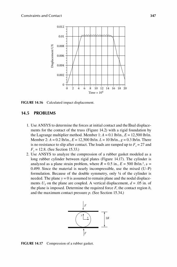
Constraints and Contact 347
14.5 proBleMS
1. Use ANSYS to determine the forces at initial contact and the final displace-ments for the contact of the truss (Figure 14.2) with a rigid foundation by the Lagrange multiplier method. Member 1: A = 0.1 lb/in., E = 12,500 lb/in. Member 2: A = 0.2 lb/in., E = 12,500 lb/in. L = 10 lb/in., g = 0.3 lb/in. There is no resistance to slip after contact. The loads are ramped up to Fx = 27 and Fy = 12.8. (See Section 15.33.)
2. Use ANSYS to analyze the compression of a rubber gasket modeled as a long rubber cylinder between rigid plates (Figure 14.17). The cylinder is analyzed as a plane strain problem, where R = 0.5 in., E = 500 lb/in.2, ν = 0.499. Since the material is nearly incompressible, use the mixed (U–P) formulation. Because of the double symmetry, only ¼ of the cylinder is needed. The plane y = 0 is assumed to remain plane and the nodal displace-ments UY on the plane are coupled. A vertical displacement, d = .05 in. of the plane is imposed. Determine the required force F, the contact region b, and the maximum contact pressure p. (See Section 15.34.)
0
0.002
0.004
0.006
0.008
0.01
0.012
Time × 1040 2 4 6 8 10 12 14 16 18 20
Disp
lace
men
t UX
fIgure 14.16 Calculated impact displacement.
2R
F
F
xy
fIgure 14.17 Compression of a rubber gasket.

348 The Finite Element Method for Mechanics of Solids with ANSYS Applications
3. Use ANSYS to solve the Hertz contact problem (Figure 14.9). The contact between the two long cylinders is analyzed by assuming double symmetry, Figure 14.13, for R1 = 10 mm, R2 = 13 mm, E1 = E2 = 30,000 N/mm2, ν1 = ν2 = 0.25. The angle defining the potential contact region is α1 = α2 = 8°. Apply d = 0.1 and determine the total force, the maximum contact pressure, and the contact region. (See Section 15.35.)
referenceS
1. Gladwell, G. M. L., Contact Problems in the Classical Theory of Elasticity, p. 1394, Sijthoff & Noordhoff, The Netherlands, 1980.
2. Timoshenko, S., and J. N. Goodier, Theory of Elasticity, 2nd ed., pp. 381–382, McGraw-Hill, New York, 1951.
BIBlIography
Kikuchi, N., and J. T. Oden, Contact problems in elasticity, A Study of Variational Inequalities and Finite Element Methods, SIAM, Philadelphia, PA, 1988.
Wriggers, P., Computational Contact Mechanics, McGraw-Hill, New York, 1951, 2nd ed., Springer-Verlag, Berlin, 2006.

349
15 ANSYS APDL Examples
15.1 anSyS InStructIonS
The instructions and examples in this chapter pertain are for version 12.1 but they are compatible with version 13. One can expect some changes with each new ver-sion. In the following instructions, C means click with the left mouse button and T means type in data, ® means ENTER. Click SAVE_DB frequently so that you can RESUM_DB if you make some unrecoverable error. Other examples of solutions using ANSYS are provided online by the HELP > ANSYS TUTORIALS button on the top toolbar.
Start the ANSYS program at your workstation. The procedure will depend on the installation on your computer system, but will be something like:
START > PROGRAMS > ANSYS 12.1 > ANSYS
A graphics window will appear as shown on the next page. A second window labeled ANSYS Output Window also appears and provides feedback throughout the analy-sis. It may be hidden behind the graphics window.
Actions by ANSYS are specified by specially formatted Commands as described in the Commands Reference Manual. These commands can be input from a file, typed on the command line above the graphics window, or by using the Graphics User Interface (GUI). The GUI makes it possible to select the required action by clicking on a menu item and entering the required data. Most items are adequately explained in the menus without reference to the help manuals. The general procedure in a stress analysis problem is as follows.
Preprocessor. The preprocessor module is used to create the geometric figure that is to be analyzed, and to mesh that body with prescribed element types and mate-rial properties. The elements are automatically merged to formulate the global stiff-ness matrix. Geometric models can also be imported from those created with CAD software such as CATIA, Parasolid, Pro/ENGINEER, SAT/ACIS, NX, SolidWorks, AutoCAD, Mechanical Desktop, and Solid Designer. The import procedure is explained in the Connection User’s Guide.
Solution. The solution module is used to apply loads and support conditions, and then solve the finite element equations directly, or by iteration, or step by step in time.
Postprocessors. A postprocessor module is used to display selected results from the solution to the finite element equations such as the components of the stress ten-sor within an element or the components of displacement of the nodes. ANSYS pro-vides two postprocessors. The General Postprocessor is used to examine the spatial solution at each step of the calculation. The Time History Postprocessor is used to display the time history of a variable such as the displacement of a node as a func-tion of time. The results can be provided in text form or as a graph. Everything that

350 The Finite Element Method for Mechanics of Solids with ANSYS Applications
appears in the graphics window can be printed, and everything that is presented as a list can be printed.
The computer program only works with numbers. It is up to the user to input the numbers in a consistent system of units. You can use any system you like. Units are mostly not mentioned in the examples in this chapter. The examples may be regarded as dealing with a nondimensional formulation.
The ANSYS software has evolved from the work of John Swanson, who established Swanson Analysis Systems in 1970. In those days, one had to use punched cards to communicate with the computer. So the input for what became the ANSYS system was a list of instructions that contained the needed information for formulated and execut-ing the finite element analysis—in effect, a special computer language that continues to underlay the formulation of problems by the computer mouse and the GUI. When you set up a problem today using the GUI, you are really generating a list of those special statements called commands. A list of commands can be seen in the Log file for each job, and ANSYS retains the option of input of the list of commands from a file or typ-ing each command on the Command Line of the GUI. In order to really understand the actions within ANSYS, one must understand the ANSYS Commands.
The classic ANSYS program has been renamed to Mechanical APDL (ANSYS Parametric Design Language) application within the Workbench environment. Extensive and detailed manuals are also accessed by the HELP menu: HELP > HELP TOPICS > CONTENTS provides a list of document sets that are available. Click on MECHANICAL APDL to see a list of manuals pertaining to mechanical analysis and a brief description of each manual. The list is alphabetical and not in the order that one would normally use the manual. Of particular interest are the fol-lowing manuals.
Basic Analysis Guide. This manual describes general tasks that apply to any type of analysis, including applying loads to a model, obtaining a solution, and using the ANSYS program’s graphics capabilities to review results.
Theory Reference for the Mechanical APDL and Mechanical Applications. This manual provides the theoretical basis for calculations in the ANSYS program, such as elements, solvers and results formulations, material models, and analysis meth-ods. By understanding the underlying theory, you can make better use of ANSYS capabilities while being aware of assumptions and limitations.
Element Reference. This manual describes all ANSYS elements in numerical order. It is the primary reference for the correct element type, input and output infor-mation, and comprehensive descriptions for every option for an element. It includes a pictorial catalog of the characteristics of each ANSYS element.
Command Reference. This manual describes all ANSYS commands in alphabeti-cal order. It is the definitive reference for correct command usage, associated GUI menu paths, product applicability, and usage notes.
Structural Analysis Guide. This reference guide describes how to perform the following structural analyses: static, modal, harmonic, transient, spectrum, buck-ling, nonlinear, material curve fitting, gasket joint simulation, fracture, composite, fatigue, p method, beams, and shells.
Modeling and Meshing Guide. This reference manual explains how to build a finite element model and mesh it.
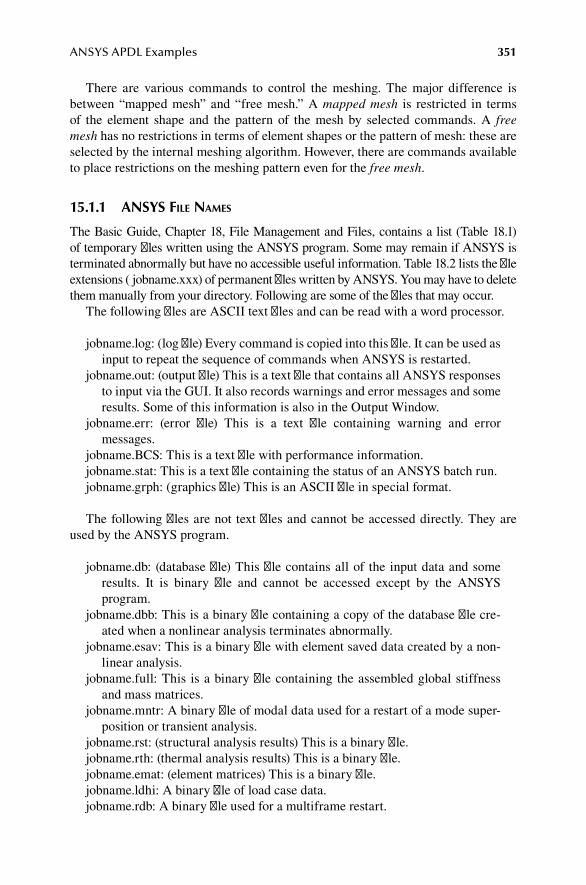
ANSYS APDL Examples 351
There are various commands to control the meshing. The major difference is between “mapped mesh” and “free mesh.” A mapped mesh is restricted in terms of the element shape and the pattern of the mesh by selected commands. A free mesh has no restrictions in terms of element shapes or the pattern of mesh: these are selected by the internal meshing algorithm. However, there are commands available to place restrictions on the meshing pattern even for the free mesh.
15.1.1 anSyS file naMeS
The Basic Guide, Chapter 18, File Management and Files, contains a list (Table 18.1) of temporary files written using the ANSYS program. Some may remain if ANSYS is terminated abnormally but have no accessible useful information. Table 18.2 lists the file extensions ( jobname.xxx) of permanent files written by ANSYS. You may have to delete them manually from your directory. Following are some of the files that may occur.
The following files are ASCII text files and can be read with a word processor.
jobname.log: (log file) Every command is copied into this file. It can be used as input to repeat the sequence of commands when ANSYS is restarted.
jobname.out: (output file) This is a text file that contains all ANSYS responses to input via the GUI. It also records warnings and error messages and some results. Some of this information is also in the Output Window.
jobname.err: (error file) This is a text file containing warning and error messages.
jobname.BCS: This is a text file with performance information.jobname.stat: This is a text file containing the status of an ANSYS batch run.jobname.grph: (graphics file) This is an ASCII file in special format.
The following files are not text files and cannot be accessed directly. They are used by the ANSYS program.
jobname.db: (database file) This file contains all of the input data and some results. It is binary file and cannot be accessed except by the ANSYS program.
jobname.dbb: This is a binary file containing a copy of the database file cre-ated when a nonlinear analysis terminates abnormally.
jobname.esav: This is a binary file with element saved data created by a non-linear analysis.
jobname.full: This is a binary file containing the assembled global stiffness and mass matrices.
jobname.mntr: A binary file of modal data used for a restart of a mode super-position or transient analysis.
jobname.rst: (structural analysis results) This is a binary file.jobname.rth: (thermal analysis results) This is a binary file.jobname.emat: (element matrices) This is a binary file.jobname.ldhi: A binary file of load case data.jobname.rdb: A binary file used for a multiframe restart.

352 The Finite Element Method for Mechanics of Solids with ANSYS Applications
15.1.2 graphic window controlS
15.1.2.1 graphics Window logoIf the ANSYS logo gets in the way, it can be removed:
PlotCtrls > Window Controls > Window Options set LOGO = Txt in Legend
15.1.2.2 display of ModelTo change the background to white background and gray elements:
PlotCtrls > Style > Colorsselect Reverse VideoPlotCtrls > Numbering >Node Numbers ON/NUM set to Numbers Only
To change to white elements with a black outline
PlotCtrls > Style > ColorsPicked Entity ColorsClab set to WHITELab set to ElementsOKPick AllPlot Ctrls > Numbering/NUM = Numbers and Colors
15.1.2.3 display of deformed and undeformed Shape White on White
Plot Ctrls >Style > Colorscheck Reverse VideoPlotCtrls > Numbering >Elem/Attrib = Element numbers/NUM = Colors and NumbersPlotCtrls > Style > ColorsEntity ColorsColor Assignment = User SpecifiedSelect ElementsSelect User Specified Color = WHITESet Entity Range = All (in first box)
15.1.2.4 adjusting graph colors
PLOT CTRLS > STYLE > COLORS > GRAPH COLORSSelect colors for curve number 1, etc.
ANSYS APDL Examples 353
15.1.2.5 printing from Windows version of anSyS
Method 1: Printing is reverse video (gray elements on a black background print as gray elements on a white background)C PRINTER LOGO (select printer)C OK (capture to printer)
Method 2: Printing is reverse videoPLOT CTRLS > CAPTURE IMAGEFILE > PRINT (select printer)C PRINT
Method 3: Printing is reverse videoPLOT CTRLS > HARD COPY > TO PRINTER (select printer)C PRINT
Method 4: Maximum flexibilityPLOT CTRLS > HARD COPY > TO FILE
This brings up a menu where you can select a file name, file type (e.g., JPEG) and options including reverse video. The file is saved in your directory.
Print the file from your directory, not from ANSYS.
15.1.2.6 Some useful notesTo get white elements and black numbers on a white background for a report, you can create black elements and white numbers on a black background and then use print method 1 or method 2.
Sometimes one needs to find get node number at a particular location. There is a way to do this without scrolling through a long list of nodes. ANSYS has a function that maps coordinates to node numbers:
C UTILITY MENU > PARAMETERS > SCALAR PARAMETERS
nodenum = node(x,y,z) [enter in selection box with actual coordi-nate values x,y,z]
C ACCEPT [under items, the value of nodenum appears]
You can enter either the node number or the parameter “nodenum” on the picking menu.
Sometimes one would like to capture a snapshot of the current screen for a report. You can press the “Print Screen” button next to the right of the F12 key and then open WORD and paste the picture into a document.
15.2 anSyS eleMentS Surf153, Surf154
ANSYS does not provide for direct input of tangential loads to solid elements. One has to make use of their surface effect elements: SURF153 for 2D problems and SURF154 for 3D problems. These elements have a variety of other uses including
354 The Finite Element Method for Mechanics of Solids with ANSYS Applications
modeling of surface tension. A description of them can be found in the Theory Reference manual. They can be viewed as a thin skin glued to the solid body that adds terms into the force stiffness and mass matrices.
SURF 153 is laid on the edge of the plane figure and is therefore a line element with the shape functions for a line element. SURF 154 is laid on the surface of a 3D element and is therefore a 2D element with the shape functions used for plane elements.
ANSYS calculates and merges the stiffness and force matrices derived from the following formulas.
K N N= ∫k Af T d ,
(15.1)
where kf is intended to represent the stiffness of an elastic support and is input as the parameter EFS in the Real Constants menu (default is zero).
M NN NN= +∫ ∫ρ t A A Ah
Td
Td d ,
(15.2)
where ρ is the surface element density and is input as a material property set, th is the thickness of the surface element input in the Real Constants menu (default zero), and Ad provides added surface mass, input as ADMSUA in the Real Constants menu (default zero).
F N p= ∫ T dA.
(15.3)
The “pressure” load p is directed in the local (x,y,z) directions according to the value of the parameter LKEY on the pressure load menu. LKEY = 2 denotes a load along x-axis, LKEY = 3 denotes load along y-axis, and LKEY = 1 denotes a load along z-axis (normal). Refer to the manual for other options for the load and for a damping matrix.
15.3 truSS exaMple
In this example, the nodes and elements are created by direct input of coordinates and node numbers.
For the truss shown in Figure 15.1, given A = 1, L = 1, E = 1, FX1 = 1, FY1 = 0, we will calculate the displacements of node 1.
a. Set job name and preferences.Login and start ANSYS APDL [wait for graphics window]C FILE > CHANGE JOBNAME [top menu bar]T a job name [in place of “file”]Select NEW LOG YesOK
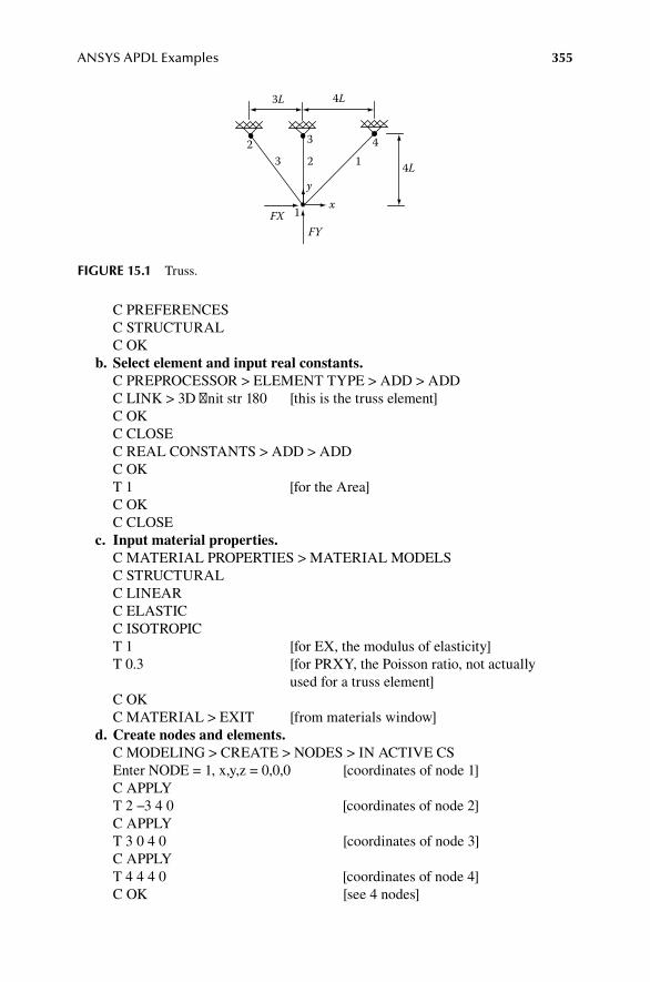
ANSYS APDL Examples 355
C PREFERENCESC STRUCTURALC OK
b. Select element and input real constants.C PREPROCESSOR > ELEMENT TYPE > ADD > ADDC LINK > 3D finit str 180 [this is the truss element]C OKC CLOSEC REAL CONSTANTS > ADD > ADDC OKT 1 [for the Area]C OKC CLOSE
c. Input material properties.C MATERIAL PROPERTIES > MATERIAL MODELSC STRUCTURALC LINEARC ELASTICC ISOTROPICT 1 [for EX, the modulus of elasticity]T 0.3 [for PRXY, the Poisson ratio, not actually
used for a truss element]C OKC MATERIAL > EXIT [from materials window]
d. Create nodes and elements.C MODELING > CREATE > NODES > IN ACTIVE CSEnter NODE = 1, x,y,z = 0,0,0 [coordinates of node 1]C APPLYT 2 −3 4 0 [coordinates of node 2]C APPLYT 3 0 4 0 [coordinates of node 3]C APPLYT 4 4 4 0 [coordinates of node 4]C OK [see 4 nodes]
4L
FXFY
4L3L
123
1
2 3
xy
4
fIgure 15.1 Truss.

356 The Finite Element Method for Mechanics of Solids with ANSYS Applications
C LIST > NODES [on top menu bar]C OKC FILE > CLOSE [if nodes are correct]C CREATE > ELEMENTSAUTO NUMBERED > THRU NODES [picking menu appears]C on nodes 1 and 4 [element 1]C APPLY [in picking window]C on nodes 1 and 3 [element 2]C APPLYC on nodes 1 and 2 [element 3]C OK [see three elements]C LIST > ELEMENTS > NODES + [top menu bar]ATTRIBUTESC FILE > CLOSE [if elements are correct]
e. Input loads and supports.C LOADS > DEFINE LOADS > APPLY > STRUCTURALC FORCE > ON NODESC on node 1C OK [in picking window]Select LAB = FX [should already be selected]Enter VALUE = 1C OK [see load vector]C STRUCTURAL DISPLACEMENT > ON NODESC on nodes 2,3,4C OKC ALL DOFEnter VALUE = 0C OK [see supports]
f. Solve equations.C SOLUTION > SOLVE > CURRENT LSCLOSE status windowC OK in solve windowCLOSE “solution is done” window
g. Examine results.C GENERAL POST PROCESSORC LIST RESULTS > NODAL SOLUTION > DOF SOLUTION > X-COMP
DISPLC OK [see UX = 6.2397; this file can be printed for the record]C CLOSEC LIST RESULTS > NODAL SOLUTION > DOF SOLUTION > Y-COMP
DISPLC OK [see UY = 0.10183; this file can be printed for the record]C FILE > CLOSEC LIST RESULTS > REACTION SOLU [ALL ITEMS selected]C OK [see list of reactions at nodes 2,3,4; this file can be printed
for the record]

ANSYS APDL Examples 357
C FILE > CLOSEC QUIT [middle menu bar]C OK
15.4 BeaM BendIng
In this example, the element data table is used to extract the element stress.Consider a cantilever beam with an end load (Figure 15.2). The beam has a rect-
angular cross section: h = 2, w = 1, A = 2, I = 2/3, E = 1000, L = 5, P = 1. Use two ele-ments as shown in Figure 15.2 to calculate the displacements, moments, and bending stress.
a. Activate ANSYS and set preferences. [default job name is “file”]See example 15.3.
b. Choose elements and materials.C PREPROCESSORenter ET,1,BEAM3 on command line [BEAM3 Element]enter KEYOPT,1,6,1 on command line [of data on member forces
and moments]enter R,1,2,2/3,2 on command line for Area, IZZ, and hC PREPROCESSOR > MATERIAL PROPS > MATERIAL MODELSC STRUCTURALC LINEARC ELASTICC ISOTROPICEnter 1000 for EX parameterC in NPRXY boxEnter 0.3 for PRXY parameter [the Poisson ratio is actually not
used]C OKC MATERIAL > EXIT
c. Create keypoints at the ends and connect them by a line.C PLOT CTRLS > NUMBERINGC box after Node numbers to turn them ONSelect Element Numbers from the ELEM/ATTRIB numbering menuC OKC PREPROCESSOR > MODELING > CREATE > KEYPOINTS > IN
ACTIVE CSEnter POINT 1 at 0,0,0
P
1 EI 2 EI 3
LL
fIgure 15.2 Bending of a beam.
358 The Finite Element Method for Mechanics of Solids with ANSYS Applications
C APPLYEnter POINT 2 at 10,0,0C OKC PREPROCESSOR > MODELING > CREATE > LINES > LINESC STRAIGHT LINEC on keypointsC OK in picking menu
d. Mesh the line.C PREPROCESSOR > MESHINGC SIZE CONTROLSC MANUAL SIZEC GLOBAL > SIZESet NDIV = 2C OKC MESHC LINESPick lineC OK [see line with two elements and three nodes]
e. Apply support conditions and loads.C SOLUTION > DEFINE LOADS > APPLY > STRUCTURALC DISPLACEMENT > ON NODESC node 2 [right end]C OKC ALL DOFC on box for VALUEST 0 for the value of the displacements and rotationOKC SOLUTION > DEFINE LOADS > APPLY > STRUCTURALC FORCE/MOMENTC ON NODESC node 1 [left end]C OKSelect FY [for LAB]C on VALUE boxT value for FY = 1C OK [force shown on the node]
f. Set solution parameters and sole equations.C UNABRIDGED MENUC SOLUTION > LOAD STEP OPTIONS > OUTPUT CONTROLSC SOLUTION PRINT OUT [to store data on element
forces]C ALL ITEMS [from Item Menu]C LAST SUBSTEPC OKC SOLUTION > SOLVE > CURRENT LSC FILE > CLOSE status window

ANSYS APDL Examples 359
C OK in solve windowC CLOSE solution window [Solution is done]
g. View results.C GENERAL POSTPROCESSORC LIST RESULTSC NODAL SOLUTIONC DOF SOLUTIONSelect Y-COMP of DisplacementC OK [see list of node displacements:
UY = 0.5 at node 1]C FILE > CLOSEC LIST RESULTSC NODAL SOLUTIONC DOF SOLUTIONSelect Z-COMP of rotationC OK [see list of rotations at each
node: −0.075 at node 1]C FILE > CLOSEC GENERAL POSTPROCESSORC ELEMENT TABLEC DEFINE TABLEC ADDEnter user label = MSelect ITEM = BY SEQ NO [scroll down to find this choice]Select SMISCEnter SMISC, 12 [this is a code number for
moment at the right end of the element]
C OK [see the element reference man-ual for the codes for BEAM3]
C CLOSEC GENERAL POSTPROCESSOR > LIST RESULTSC ELEM TABLE DATASelect MC OK [see M = 5 for element 1 and M = 10
for element 2]C FILE > CLOSEC GENERAL POSTPROCESSOR > ELEMENT TABLE > DEFINE
TABLEC ADDEnter user label = SSelect ITEM = BY SEQ NO [scroll down to find this choice]Select LSEnter LS,6 [this is a code number for bend-
ing stress at the right end of the element]

360 The Finite Element Method for Mechanics of Solids with ANSYS Applications
C OKC CLOSEC GENERAL POSTPROCESSOR > LIST RESULTSC ELEM DATA TABLE [deselect M]Select SC OK [see S = 15 for element 2]C FILE > CLOSEC QUITC OK
15.5 BeaM WIth a dIStrIButed load
In this example, a nonuniform pressure load is introduced.A cantilever beam with a linearly varying load (Figure 15.3) and a rectangular
cross section has the following dimensions: h = 1, w = 1, A = 1, I = 1/12, E = 30 × 106, L = 10, p = 1. We are to calculate the displacements. One element gives the exact
solution: UY = = × −11120
1130
104
4pL
EI downward at the end.
a. Activate ANSYS and set preferences.See example 15.3.
b. Choose elements and materials.C PREPROCESSORenter ET,1,BEAM3 on command line [BEAM3 Element]enter R,1,1,1/12,1 on command line for Area, IZZ, and hC PREPROCESSOR > MATERIAL PROPS > MATERIAL MODELSC STRUCTURALC LINEARC ELASTICC ISOTROPICEnter 30e6 for EX parameter C in NPRXY boxEnter 0.3 for PRXY parameter [the Poisson ratio is actually not used]C OKC MATERIAL > EXIT
c. Create nodes and elements.C PREPROCESSOR > MODELING > CREATE > NODES > IN ACTIVE CSEnter POINT 1 at 0,0,0
p
LEI
fIgure 15.3 Bending of a beam with distributed load.

ANSYS APDL Examples 361
C APPLYEnter POINT 2 at 10,0,0C OKC PREPROCESSOR > MODELING > CREATE > ELEMENTSC AUTO-NUMBERED > THRU NODESC on node 1 then node 2 [beam element: I = 1, J = 2]C OK in picking menu
d. Apply support conditions and loads.C SOLUTION > DEFINE LOADS > APPLY > STRUCTURALC DISPLACEMENT > ON NODESC node 1 [left end, or Type 1 in box on pick-
ing menu]C OKC ALL DOFC on box for VALUEST 0 [for the value of the displacements and rotation]OKC SOLUTION > DEFINE LOADS > APPLY > STRUCTURALC PRESSURE > ON BEAMSC on beam element [or Type 1 in box on picking menu]C OK [load menu appears]Enter LKEY = 1, VALI = 0, [load varies linearly from node I to VALJ = 1 node J]C OK [representative force shown on the
element]e. Solve the equations.
C SOLUTION > SOLVE > CURRENT LSC CLOSE status windowC OK in solve windowC CLOSE solution window [solution is done]
f. Extract results.C GENERAL POSTPROCESSORC LIST RESULTSC NODAL SOLUTIONC DOF SOLUTIONSelect Y-COMP of DisplacementC OK [see list of node displacements:
UY = −0.36667 × 10⁻³ at node 2]C FILE > CLOSEC QUITC OK
15.6 one trIangle
In this example, nodes are created by specifying coordinates and elements are cre-ated by picking nodes.

362 The Finite Element Method for Mechanics of Solids with ANSYS Applications
The analysis is to check the element stiffness matrix for a plane stress triangle (Figure 15.4) as generated by the Plane 182 element. In nondimensional units, E = 16, ν = 1/3, μ = 6.
a. Activate ANSYS and set preferences.See example 15.3.
b. Select element and material properties.C PREPROCESSOR > ELEMENT TYPE > ADDC ADD in the new windowC SOLID C 4 NODE 182 [the triangle is a special case of
this element]C OKC CLOSE C PREPROCESSOR > MATERIAL PROPS > MATERIAL MODELSC STRUCTURALC LINEARC ELASTICC ISOTROPICT 16 for EX parameterC in PRXY boxT 1/3 for PRXY parameter [ANSYS converts this to five sig-
nificant figures]C OK [μ = 6]C MATERIAL > EXIT
c. Create nodes and elements.C PLOT CTRLS > NUMBERING [top line menu]C box after Node numbers to turn them ONC OKC PREPROCESSOR > MODELING > CREATE > NODES > IN ACTIVE
CST node = 1, x = 0, y = 0C APPLYT node = 2, x = 1, y = 0C APPLY
1.0
x1
y
2
3
0.5
fIgure 15.4 Plane stress triangle.

ANSYS APDL Examples 363
T node = 3, x = 0.5, y = 0.5C OK C PREPROCESSOR > MODELING > CREATE > ELEMENT > C AUTO NUMBERED > THRU NODESC nodes 1,2,3 [specifying only three nodes implies
a triangle]C OK
d. Apply boundary conditions.C SOLUTION > DEFINE LOADS > APPLY > STRUCTURAL C DISPLACEMENT > ON NODESC nodes 2 and 3C APPLYC ALL DOF if it is not selected alreadyC on box for VALUEST 0 for the value of the displacement componentsC APPLYC node 1APPLYC UY [deselect ALL DOF]C APPLYC node 1OKC UY [to deselect UY]C UXC on VALUE boxT value for UX of 1C OKC LIST > LOADS > DOF CONSTRAINTS [Utility menu at top]C ON ALL LINES [check boundary
conditions]C FILE > CLOSE
e. Solve for displacements and stresses.C SOLUTION > SOLVE > CURRENT LSC CLOSE information windowC OK in Solve window C YES in warning window [ANSYS suggests reduced
integration]C CLOSE on information window [solution is done]
f. Display results.C GENERAL POST PROC > LIST RESULTS > REACTION SOLUC OK to get a list of nodal forces that [this can be compared
comprise column one of the stiffness with column 1 of k1, matrix. Equation 4.45]
C FILE > CLOSEC QUITC OK

364 The Finite Element Method for Mechanics of Solids with ANSYS Applications
15.7 plane StreSS exaMple uSIng trIangleS
This example illustrates the use of the COPY command to create nodes and elements and the box method in the picking menu.
The given problem is the short beam (Figure 15.5). The solution for the corner displacement is tabulated in Table 4.3. In nondimensional units: a = 1, p = 1, E = 1, ν = 1/3.
a. Activate ANSYS and set preferences.See example 15.3.
b. Choose element and material.C PREPROCESSOR > ELEMENT TYPE > ADDC ADD in the new windowC SOLID C 4 NODE 182 [PLANE182 element]C OK [the constant strain triangle is a special case
this element]C CLOSE C PREPROCESSOR > MATERIAL PROPS > MATERIAL MODELSC STRUCTURALC LINEARC ELASTICC ISOTROPICT 1 for EX parameter [nondimensional parameters]C in PRXY boxT 1/3 for PRXY parameter [PR is Poisson ratio]C OKC MATERIAL > EXIT
c. Create nodes and elements.C PREPROCESSOR > MODELING > CREATEC NODES > IN ACTIVE CST 1 0 0 0 [for Node,X,Y,Z]C APPLY
1/8 1/81/4 1/4 1/4
C
fIgure 15.5 Short beam, 64 triangles.

ANSYS APDL Examples 365
T 2 0.25 0 0 [for Node,X,Y,Z]C APPLYT 11 0.25 0.25 0 [for Node,X,Y,Z]C APPLYT 10 0 0.25 0 [for Node,X,Y,Z]C APPLYT 6 0.125 0.125 0 [note the numbering, chosen for the copy
command]C OKC PREPROCESSOR > MODELING > CREATEC ELEMENTS > AUTO NUMBERED > THRU NODESC nodes 1 then 2 then 6 [specifying three nodes implies a triangle]APPLYC nodes 2 then 11 then 6APPLYC nodes 11 then 10 then 6APPLYC nodes 10 then 1 then 6OKC PREPROCESSOR > MODELING > COPYC ELEMENTS > AUTO NUMBEREDC PICK ALLT 4 for ITIME [leave NINC = 1]T 0.25 for DX [creating bottom row of elements]C OKC PREPROCESSOR > MODELING > COPYC ELEMENTS > AUTO NUMBEREDC PICK ALLT 4 for ITIMET 9 for NINCT 0 for DXT 0.25 for DYC OK [creating columns of
elements]C PLOT CTRLS > NUMBERING [top line menu]C box after Node numbers to turn them ONC OK
d. Apply boundary conditions.C PREPROCESSOR > LOADS > DEFINE LOADS > APPLYC STRUCTURAL > DISPLACEMENT > ON NODESC BOX [on picking menu]DRAW A BOX AROUND THE BOTTOM NODES BY CLICK AND
DRAGC OKC ALL DOF [if it is not selected already]C on box for VALUES
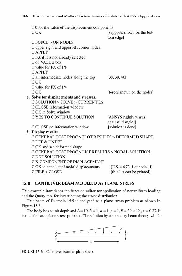
366 The Finite Element Method for Mechanics of Solids with ANSYS Applications
T 0 for the value of the displacement componentsC OK [supports shown on the bot-
tom edge]C FORCE > ON NODESC upper right and upper left corner nodesC APPLYC FX if it is not already selectedC on VALUE boxT value for FX of 1/8C APPLYC all intermediate nodes along the top [38, 39, 40]C OKT value for FX of 1/4 C OK [forces shown on the nodes]
e. Solve for displacements and stresses.C SOLUTION > SOLVE > CURRENT LSC CLOSE information windowC OK in Solve windowC YES TO CONTINUE SOLUTION [ANSYS rightly warns
against triangles]C CLOSE on information window [solution is done]
f. Display results.C GENERAL POST PROC > PLOT RESULTS > DEFORMED SHAPEC DEF & UNDEF C OK and see deformed shapeC GENERAL POST PROC > LIST RESULTS > NODAL SOLUTIONC DOF SOLUTIONC X-COMPONENT OF DISPLACEMENTC OK to get a list of nodal displacements [UX = 6.7341 at node 41]C FILE > CLOSE [this list can be printed]
15.8 cantIlever BeaM Modeled aS plane StreSS
This example introduces the function editor for application of nonuniform loading and the Query tool for investigating the stress distribution.
This beam of Example 15.5 is analyzed as a plane stress problem as shown in Figure 15.6.
The body has a unit depth and L = 10, h = 1, w = 1, p = 1, E = 30 × 106, ν = 0.27. It is modeled as a plane stress problem. The solution by elementary beam theory, which
L
p
h
fIgure 15.6 Cantilever beam as plane stress.

ANSYS APDL Examples 367
neglects shear deformations, is a tip displacement with value 11pL4/120 EI = 0.367 × 10⁻³ and a maximum bending stress of Mc/I = 2pL2/wh2 = 200.
a. LOGIN and launch ANSYS.See example 15.3.
b. Define elements and materials.C PREPROCESSOR > ELEMENT TYPE > ADDC ADD in the new windowC SOLID Select 8 NODE 183 [PLANE183 element]C OK [plane stress is the default]C CLOSE C PREPROCESSOR > MATERIAL PROPS > MATERIAL MODELSC STRUCTURALC LINEARC ELASTICC ISOTROPICT 30e6 for EX parameterC in PRXY boxT 0.27 for PRXY parameter [PR is Poisson ratio]C OKC MATERIAL > EXIT
c. Create geometric figure.C PREPROCESSOR > MODELING > CREATEC AREAS > RECTANGLE > BY DIMENSIONST 0 10 0 1 for X1,X2,Y1,Y2C OK and the region appears
d. Mesh figure.C PLOT CTRLS > NUMBERING [top line menu]C box after Node numbers to turn them ONC OKC PREPROCESSOR > MESHING > MESH > AREAS > FREEC PICK ALL [mesh using default size]
[2 high by 15 wide mesh appears with node numbers]
e. Define load distribution function.C PARAMETERS > FUNCTIONS > [on top utility menu] DEFINE/EDITC 0.1*Select X in the drop menu currently [Result = 0.1*{X}] showing TIMEC GRAPH [click INV if GRAPH is not a cur-
rent label in the gray buttons]Enter X-Axis Range: 0 to 10C GRAPH [see graph of function]C CLOSE Plot Information window [may be behind graphics window]

368 The Finite Element Method for Mechanics of Solids with ANSYS Applications
C FILE > SAVE [in Function Editor window]Enter File name PSR [saved as PSR.func]C SAVEC FILE > CLOSEC PARAMETERS > FUNCTIONS > READ FROM FILEEnter PSR.funcC OPENEnter Table parameter name = PRESSC OKC PLOT > ELEMENTS
f. Apply boundary conditions.C SOLUTION > DEFINE LOADS > APPLY > STRUCTURALC DISPLACEMENT > ON LINESC left edge of the modelC OKC ALL DOF if it is not selected alreadyC on box for VALUEST 0 for the value of the displacement componentsC OK [supports shown on the left edge]C SOLUTION > DEFINE LOADS > APPLY > STRUCTURAL C PRESSURE > ON LINESC top line [Y = 1]C OKSelect EXISTING TABLE from SFL menuOKSelect PRESSOK [arrow appears to indicated pressure load]
g. Solve finite element equations.C SOLUTION > SOLVE > CURRENT LSC CLOSE information windowC OK in Solve window C FILE > CLOSE on information window [solution is done]
h. Display results.C GENERAL POST PROC > PLOT RESULTS > DEFORMED SHAPEC DEF & UNDEFC OK and see deformed shapeC PLOT > ELEMENTSC GENERAL POST PROC > LIST RESULTS > NODAL SOLUTIONC DOF SOLUTIONC Y-COMPONENTC OK to get a list of nodal displacements [UX = −0.36893 × 10⁻³ at
node 34]C FILE > CLOSEC GENERAL POST PROC > QUERY RESULTS > SUBGRID SOLUC STRESSC X-DIRECTION

ANSYS APDL Examples 369
C OKC node 36 [maximum bending
stress = 202.57]C OK [not accurate with this few
elements]
15.9 plane StreSS: pure BendIng
In this example, the use of symmetry and antisymmetry to apply boundary condi-tions is introduced.
The problem diagrammed in Figure 15.7. One-quarter of the body is analyzed using symmetry conditions. In nondimensional units: a = 2, b = 2, p = 1, E = 1, ν = 0.3. To prevent rigid displacement we set u(0,0) = v(0,0) = 0. An approximate solution is obtained by using a four-node element as described in Section 5.1.2.
a. Activate ANSYS and set the job name and preferences.See example 15.3.
b. Choose element and material.C PREPROCESSOR > ELEMENT TYPE > ADDC ADD in the new windowC SOLIDC 4 NODE 182 [Plane182
element]C OKC CLOSEC PREPROCESSOR > MATERIAL PROPS > MATERIAL MODELSC STRUCTURALC LINEARC ELASTICC ISOTROPICT 1 for EX parameterC in PRXY boxT 0.3 for PRXY parameterC OKC MATERIAL > EXIT
p
yx A
S b/2
a/2
fIgure 15.7 Plane stress: pure bending.

370 The Finite Element Method for Mechanics of Solids with ANSYS Applications
c. Create geometric figure.C PREPROCESSOR > MODELING > CREATEC AREAS > RECTANGLE > BY DIMENSIONST 0 1 0 1 for X1,X2,Y1,Y2C OK and the region appears
d. Mesh figure.C PLOT CTRLS > NUMBERING [top line menu]C box after Node numbers to turn them ONC ELEMENT NUMBERS from Elem pull-down menuC NUMBERS ONLY from /NUM pull-down menuC OKC PREPROCESSOR > MESHING > SIZE CONTROLSC MANUAL SIZE > LINES > PICKED LINESPick top and bottomC APPLYC box for NDIVT 2 in NDIV box to mesh with 2 divisions per sideC APPLYPick left and right endsC OKT 2 in NDIV box to mesh with 2 divisions per sideC OKC PREPROCESSOR > MESHING > MESH > AREAS > FREEC PICK ALL [2 × 2 grid of
square elements]e. Define load distribution functions.
C PARAMETERS > FUNCTIONS > DEFINE/EDIT [on top utility menu]
C 1*Select Y in the drop menu currently [Result = 1*{Y}]showing TIMEC FILE > SAVE [in Function Editor
window]Enter File name: SIGX [saved as SIGX.func]C SAVEC FILE > CLOSEC PARAMETERS > FUNCTIONS > READ FROM FILESelect SIGX.funcC OPENEnter Table parameter name = SIGXC OK
f. Apply boundary conditions.C SOLUTION > DEFINE LOADS > APPLY > STRUCTURALC DISPLACEMENT > ON NODESC on node at the originC OK

ANSYS APDL Examples 371
Select ALL DOF [UX = 0 and UY = 0 at the origin]
C on box for VALUEST 0 for the value of the displacement componentsC OKC SOLUTION > DEFINE LOADS > APPLY > STRUCTURAL C SYMMETRY B.C. > ON LINESC RIGHT EDGEC OKC ANTISYMM B.C. > ON LINESC BOTTOM EDGEC OKSOLUTION > DEFINE LOADS > APPLY > STRUCTURALPRESSURE > ON LINESC on the left edgeC OKSelect EXISTING TABLE from SFE drop down menuC OK [check that SIGX is selected]C OK [pressure equals a compres-
sive stress] [you can check on the loads by
LIST > LOADS > SURFACE > ON ALL LINES]
g. Get solution.C SOLUTION > SOLVE > CURRENT LSC FILE > CLOSE status windowC OK in Solve window C CLOSE on information window [solution is done]
h. Display results.C GENERAL POST PROC > LIST RESULTS > NODAL SOLUTIONC STRESSC X-COMPONENTC OK [SX = −0.98985 at node 4, SX = −0.49029
at node 5]C FILE > CLOSEC QUITC OK
15.10 plane StraIn BendIng exaMple
The SURF element is introduced for application of shear loads. A change in material properties without repeating the entire analysis is also demonstrated.
This example is a solution of the problem described in Section 5.1.3. The com-plete structure is shown in Figure 15.8, but the analysis uses only the upper half and antisymmetry on the line y = 0. In nondimensional terms: c = 2, L = 16, P = 32, E = 8192, ν = 0.3.
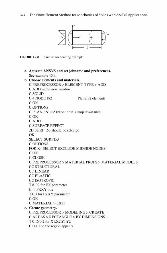
372 The Finite Element Method for Mechanics of Solids with ANSYS Applications
a. Activate ANSYS and set jobname and preferences.See example 15.3.
b. Choose elements and materials.C PREPROCESSOR > ELEMENT TYPE > ADDC ADD in the new windowC SOLID C 4 NODE 182 [Plane182 element]C OKC OPTIONSC PLANE STRAIN on the K3 drop down menuC OKC ADDC SURFACE EFFECT 2D SURF 153 should be selectedOKSELECT SURF153C OPTIONSFOR K4 SELECT EXCLUDE MIDSIDE NODESC OKC CLOSE C PREPROCESSOR > MATERIAL PROPS > MATERIAL MODELSCC STRUCTURALCC LINEARCC ELASTICCC ISOTROPICT 8192 for EX parameterC in PRXY boxT 0.3 for PRXY parameter C OKC MATERIAL > EXIT
c. Create geometry.C PREPROCESSOR > MODELING > CREATEC AREAS > RECTANGLE > BY DIMENSIONST 0 16 0 2 for X1,X2,Y1,Y2C OK and the region appears
τxy
τxy
L
c
cx
y
σx
fIgure 15.8 Plane strain bending example.

ANSYS APDL Examples 373
d. Mesh figure.C PLOT CTRLS > NUMBERING [top line menu]C box after Node numbers to turn them ONSelect ELEMENT NUMBERSSelect NUMBERS ONLYC OKC PREPROCESSOR > MESHING > SIZE CONTROLSC MANUAL SIZE > LINES > PICKED LINESPick top and bottomC APPLYC box for NDIVT 8 in NDIV box to mesh with 8 divisions per sideC APPLYPick left and right endsC OKT 4 in NDIV box to mesh with 4 divisions per sideC OKPREPROCESSOR > MESHING > MESH > AREAS > FREEC PICK ALL [creates 4 × 8 mesh]MODELING > CREATE > ELEMENTS > ELEM ATTRIBUTESSelect TYPE = 2 SURF 153C OKSURF/CONTACT > SURF TO SURFC OK (Tlab = Top surface)C BOX [on picking menu]Draw box around nodes on RIGHT edge by holding down mouse button
and draggingC APPLYC OKC BOXDraw box around nodes on LEFT edge by holding down the mouse button
and draggingC OKLIST > ELEMENTS > NODESCheck the I and J nodes of new elements of type 2 [down on the
right and up on the left]
CLOSEe. Define load distribution functions.
PARAMETERS > FUNCTIONS > DEFINE/EDIT [on top utility menu]
C 96*Select Y in the drop menu currently showing TIME [Result = 96*{Y}]FILE > SAVE [in Function
Editor window]
374 The Finite Element Method for Mechanics of Solids with ANSYS Applications
Enter File name: MOMENT [saved as MOMENT.func]
SAVEFILE > CLOSEPARAMETERS > FUNCTIONS > READ FROM FILESelect MOMENT.funcOPENEnter Table parameter name = MOMENTOKPARAMETERS > FUNCTIONS > DEFINE/EDIT [on top utility menu]C − 12 + 3 * [note minus sign]Select Y in the drop menu currently showing TIMEC *Again, select Y in the drop menu [Result =
>12+3*{Y}*{Y}]]C FILE > SAVE [in Function
Editor window]Enter File name = SHEAR [saved as SHEAR.
func]C SAVEC FILE > CLOSEC PARAMETERS > FUNCTIONS > READ FROM FILESelect SHEAR.funcC OPENEnter Table parameter name = shearC OK
f. Apply boundary conditions.C SOLUTION > DEFINE LOADS > APPLY > STRUCTURALC DISPLACEMENT > ON LINESC bottom edge of the modelC OKSelect UXC on box for VALUEST 0 for the value of the displacement componentsC OKC DISPLACEMENT > ON NODESPick node in lower left cornerC APPLYSelect UYT value = 0C APPLYPick node in upper left cornerC OKSelect UX [deselect UY]C OKC SOLUTION > DEFINE LOADS > APPLY > STRUCTURAL
ANSYS APDL Examples 375
C PRESSURE > ON ELEMENTSC BOX (on picking menu)Draw a box around the surface elements on the right edgeC OKSET LKEY = 2 [tangential load on the element]Select EXISTING TABLE from SFE drop down menuC OKSelect SHEARC OK [no indication of loading]C SOLUTION > DEFINE LOADS > APPLY > STRUCTURALC PRESSURE > ON ELEMENTSC BOX (on picking menu)Draw a box around the surface elements on the left edgeC OKSET LKEY = 2 [tangential load on the element]Select EXISTING TABLE from SFE drop down menuC OKSelect SHEARC OKC SOLUTION > DEFINE LOADS > APPLY > STRUCTURALC PRESSURE > ON ELEMENTSC BOX (on picking menu)Draw a box around the surface elements on the left edgeC OKSET LKEY = 1 [pressure load on the element]Select EXISTING TABLE from SFL drop down menuC OKSelect MOMENTC OK
[you can check on the loads by LIST > LOADS > SURFACE > ON ELEMENTS]
g. Get solution.C SOLUTION > SOLVE > CURRENT LSC CLOSE information windowC OK in Solve window C CLOSE on information window [solution is done]
h. Display results.C GENERAL POST PROC > PLOT RESULTS > DEFORMED SHAPEC OK and check deformed shapeC GENERAL POST PROC > LIST RESULTS > NODAL SOLUTIONC DOF SOLUTIONC Y-COMPONENTC OK to get a list of nodal displacements [UY = 0.85774 at lower
right corner]
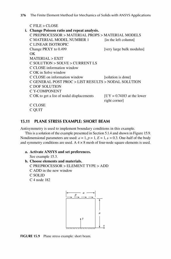
376 The Finite Element Method for Mechanics of Solids with ANSYS Applications
C FILE > CLOSEi. Change Poisson ratio and repeat analysis.
C PREPROCESSOR > MATERIAL PROPS > MATERIAL MODELSC MATERIAL MODEL NUMBER 1 [in the left column]C LINEAR ISOTROPICChange PRXY to 0.499 [very large bulk modulus]OKMATERIAL > EXITC SOLUTION > SOLVE > CURRENT LSC CLOSE information windowC OK in Solve window C CLOSE on information window [solution is done]C GENERAL POST PROC > LIST RESULTS > NODAL SOLUTIONC DOF SOLUTIONC Y-COMPONENTC OK to get a list of nodal displacements [UY = 0.74183 at the lower
right corner]C CLOSEC QUIT
15.11 plane StreSS exaMple: Short BeaM
Antisymmetry is used to implement boundary conditions in this example.This is a solution of the example presented in Section 5.1.4 and shown in Figure 15.9.
Nondimensional parameters are used: a = 1, p = 1, E = 1, ν = 0.3. One-half of the body and symmetry conditions are used. A 4 × 8 mesh of four-node square elements is used.
a. Activate ANSYS and set preferences.See example 15.3.
b. Choose elements and materials.C PREPROCESSOR > ELEMENT TYPE > ADDC ADD in the new windowC SOLID C 4 node 182
y
x
a
ap
fIgure 15.9 Plane stress example: short beam.
ANSYS APDL Examples 377
C OKC ADDC SURFACE EFFECT 2D SURF 153 should be selectedOKSELECT SURF153C OPTIONSFOR K4 SELECT EXCLUDE MIDSIDE NODESC OKC CLOSE C PREPROCESSOR > MATERIAL PROPS > MATERIAL MODELSC STRUCTURALC LINEARC ELASTICC ISOTROPICT 1 for EX parameterC in PRXY boxT 0.3 for PRXY parameter C OKC MATERIAL > EXIT
c. Create geometry.C PREPROCESSOR > MODELING > CREATEC AREAS > RECTANGLE > BY DIMENSIONST 0 0.5 0 1 for X1,X2,Y1,Y2C OK and the region appears
d. Mesh figure.C PLOT CTRLS > NUMBERING [top line menu]C box after Node numbers to turn them ONC OKC PREPROCESSOR > MESHING > SIZE CONTROLSC MANUAL SIZE > GLOBAL > SIZEC box for NDIVT 0.125 in SIZE box to control element sizeC OKPREPROCESSOR > MESHING > MESH > AREAS > FREEC PICK ALL [4 × 8 square mesh appears with
node numbers]C PREPROCESSOR > MODELING > CREATE > ELEMENTSC ELEMENT ATTRIBUTESSelect 2 SURF 153 on TYPE menuOKC SURF / CONTACT > SURF TO SURFC OK [accept TLAB = TopSurface]C BOX on picking menuUse cursor to draw a box around the top edgeC OK in picking menu

378 The Finite Element Method for Mechanics of Solids with ANSYS Applications
e. Apply boundary conditions.C SOLUTION > DEFINE LOADS > APPLY > STRUCTURALC DISPLACEMENT > ON LINESC bottom edge of the modelC OKC ALL DOF if it is not selected alreadyC on box for VALUEST 0 for the value of the displacement componentsC OK [supports shown on the bottom
edge]C SOLUTION > DEFINE LOADS > APPLY > STRUCTURALC ANTI-SYMM > ON LINESC left edge of the modelC OKC SOLUTION > DEFINE LOADS > APPLY > STRUCTURAL C PRESSURE > ON ELEMENTSC BOX in picking menuC draw around top edge C OKEnter LKEY = 2Enter VALUE = 1C OK [close Warning window]
f. Solve for displacements and stresses.C SOLUTION > SOLVE > CURRENT LSC CLOSE information windowC OK in Solve windowC CLOSE on information window [solution is done]
g. Display results.C GENERAL POST PROC > PLOT RESULTS > DEFORMED SHAPEC DEF & UNDEF C OK and see deformed shapeC GENERAL POST PROC > LIST RESULTS > NODAL SOLUTIONC DOF SOLUTIONC X-COMPONENTC OK to get a list of nodal displacements [UX = 7.1207 at node 6]C CLOSEC GENERAL POST PROC > LIST RESULTS > NODAL SOLUTIONC STRESSC Y-COMPONENTC OK to get a list of stress components [SY = −7.3741 at node 2]
extrapolated to each node C CLOSE [remember that there is
actually a singularity at node 2]
C QUITC OK

ANSYS APDL Examples 379
15.12 Sheet WIth a hole
Use of the Boolean operator to subtract areas, use of the Mesh Tool, and Refinement of the Mesh are introduced.
A sheet with a central hole (Figure 15.10) is stretched by a uniform edge stress S resulting in a stress concentration at the hole. In nondimensional variables: S = 100, a = 20, b = 10, r = 5, E = 1, ν = 0.3.
15.12.1 Solution procedure
a. Activate ANSYS, change job name, and set preferences to structural.See example 15.3.
b. Choose element and material.C PREPROCESSOR > ELEMENT TYPE > ADDC ADD in the new windowC SOLID C 4 node 182 C OKC CLOSE C PREPROCESSOR > MATERIAL PROPS > MATERIAL MODELSC STRUCTURALC LINEARC ELASTICC ISOTROPICT 1 for EX parameterC in PRXY boxT 0.3 for PRXY parameter C OKC MATERIAL > EXIT
c. Create the body by first creating a rectangle then subtracting the circu-lar area.C PREPROCESSOR > MODELING > CREATEC AREAS > RECTANGLE > BY 2 CORNERS
2a
y
xr
S2b
fIgure 15.10 Sheet with a hole.

380 The Finite Element Method for Mechanics of Solids with ANSYS Applications
Enter WP X = 0, WP Y = 0 [this establishes the origin of the working plane]
Enter Width = 20, Height = 10 [dimensions of the rectangle]C OK and the rectangular region appearsC PREPROCESSOR > MODELING > CREATEC AREAS > CIRCLE > SOLID CIRCLEEnter WP X = 0, WP Y = 0 [center of the circular area]Enter Radius = 5C OK [circular area appears]C PLOT CTRLS > NUMBERING [top line menu]C AREA NUMBERING [rectangle is A1, circle is A2]C OKC PREPROCESSOR > MODELING > OPERATE > BOOLEANS C SUBTRACT > AREASPICK RECTANGULAR AREAC OKPICK CIRCLULAR AREAC OK [body appears as area A3]
d. Mesh the body.C PREPROCESSOR > [mesh tool menu appears]
MESHING > MESH TOOLSelect Smart Size [note: slider sets at 6 by default]C MESH [near the bottom of mesh tool
menu]C Pick All [coarse mesh appears]C REFINE [Refine at Elements selected]Pick elements along the arc of the circleOK [level 1 selected]OK [refined mesh appears]
e. Apply boundary conditions.C SOLUTION > DEFINE LOADS > APPLY > STRUCTURAL >
DISPLACEMENTC SYMMETRY > ON LINESC bottom edge and the left edge of the model C OKC SOLUTION > DEFINE LOADS > APPLY > STRUCTURAL C PRESSURE > ON LINESC RIGHT EDGE C OKC on VALUE boxT −100 for the value [negative pressure is
tension]C OK
f. Solve for displacements and stresses.C SOLUTION > SOLVE > CURRENT LSC CLOSE information window
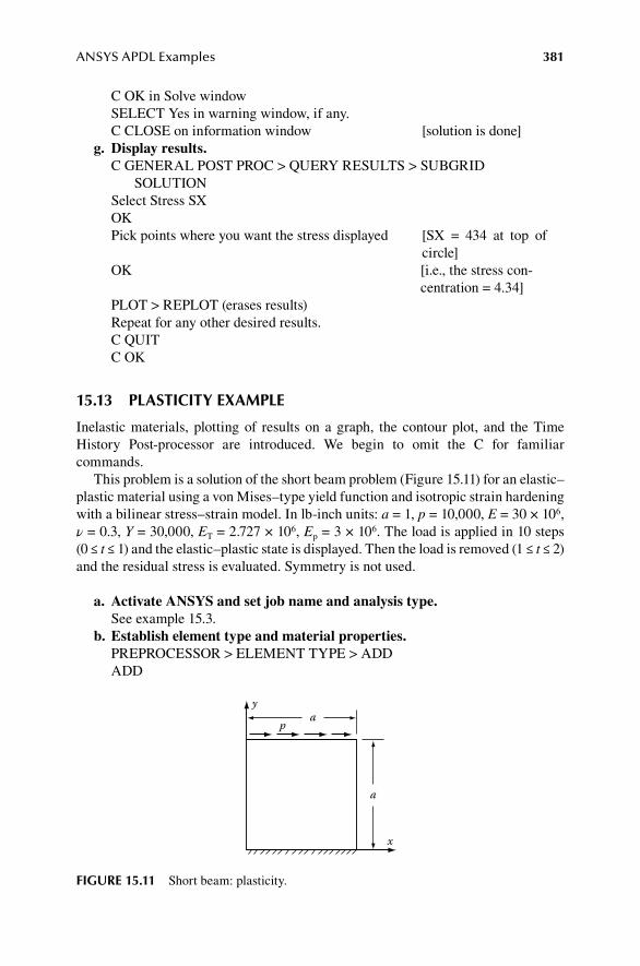
ANSYS APDL Examples 381
C OK in Solve window SELECT Yes in warning window, if any.C CLOSE on information window [solution is done]
g. Display results.C GENERAL POST PROC > QUERY RESULTS > SUBGRID
SOLUTIONSelect Stress SXOKPick points where you want the stress displayed [SX = 434 at top of
circle]OK [i.e., the stress con-
centration = 4.34]PLOT > REPLOT (erases results)Repeat for any other desired results.C QUITC OK
15.13 plaStIcIty exaMple
Inelastic materials, plotting of results on a graph, the contour plot, and the Time History Post-processor are introduced. We begin to omit the C for familiar commands.
This problem is a solution of the short beam problem (Figure 15.11) for an elastic–plastic material using a von Mises–type yield function and isotropic strain hardening with a bilinear stress–strain model. In lb-inch units: a = 1, p = 10,000, E = 30 × 106, ν = 0.3, Y = 30,000, ET = 2.727 × 10⁶, Ep = 3 × 10⁶. The load is applied in 10 steps (0 ≤ t ≤ 1) and the elastic–plastic state is displayed. Then the load is removed (1 ≤ t ≤ 2) and the residual stress is evaluated. Symmetry is not used.
a. Activate ANSYS and set job name and analysis type.See example 15.3.
b. Establish element type and material properties.PREPROCESSOR > ELEMENT TYPE > ADDADD
y
pa
a
x
fIgure 15.11 Short beam: plasticity.

382 The Finite Element Method for Mechanics of Solids with ANSYS Applications
SOLIDQUAD 4node 182APPLYSURFACE EFFECT > 2D STRUCTURAL 153OKC SURF 153OPTIONSFOR K4 SELECT EXCLUDE MIDSIDE NODESOKCLOSEPREPROCESSOR > MATERIAL PROP > MATERIAL MODELSSTRUCTURALNONLINEARINELASTICRATE INDEPENDENTISOTROPIC HARDENING PLASTICITYMISES PLASTICITYBILINEAR [request for elastic properties
appears]OKEnter 30e6 for EX parameterEnter 0.3 for PRXY parameterOKEnter 30000 for the Yield StrsEnter 2.727e6 for the Tang ModOKMATERIAL > EXITPLOT on the top menuDATA TABLESOK [plots stress–strain diagram]
c. Create geometry.PREPROCESSOR > MODELING > CREATEAREAS > RECTANGLE > BY DIMENSIONSEnter 0 1 0 1 for X1,X2,Y1,Y2OK and the region appears
d. Mesh body.PLOT CTRLS > NUMBERING [top line menu]C box after Node numbers to turn them ONOKPREPROCESSOR > MESHING > MESHTOOLSMART SIZESet slider to 4 [produces a 17 × 17 element mesh]MESH [at the bottom of mesh tool menu] PICK ALL [the coarse mesh appears]C REFINE at Elements on mesh tool [it may be hidden behind graphics
window]
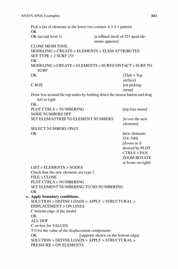
ANSYS APDL Examples 383
Pick a fan of elements at the lower two corners 4-3-2-1 patternOKOK (accept level 1) [a refined mesh of 523 quad ele-
ments appears]CLOSE MESH TOOLMODELING > CREATE > ELEMENTS > ELEM ATTRIBUTESSET TYPE = 2 SURF 153OKMODELING > CREATE > ELEMENTS > SURF/CONTACT > SURF TO
SURFOK [Tlab = Top
surface]C BOX [on picking
menu]Draw box around the top nodes by holding down the mouse button and drag
left to rightOKPLOT CTRLS > NUMBERING [top line menu]NODE NUMBERS OFFSET ELEM/ATTRIB TO ELEMENT NUMBERS [to see the new
elements]SELECT NUMBERS ONLYOK [new elements
524–540] [Zoom in if
desired by PLOT CTRLS > PAN ZOOM ROTATE or Icons on right]
LIST > ELEMENTS > NODESCheck that the new elements are type 2FILE > CLOSEPLOT CTRLS > NUMBERING SET ELEMENT NUMBERING TO NO NUMBERING OK
e. Apply boundary conditions.SOLUTION > DEFINE LOADS > APPLY > STRUCTURAL >DISPLACEMENT > ON LINESC bottom edge of the modelOKALL DOF C on box for VALUEST 0 for the value of the displacement componentsOK [supports shown on the bottom edge]SOLUTION > DEFINE LOADS > APPLY > STRUCTURAL >PRESSURE > ON ELEMENTS
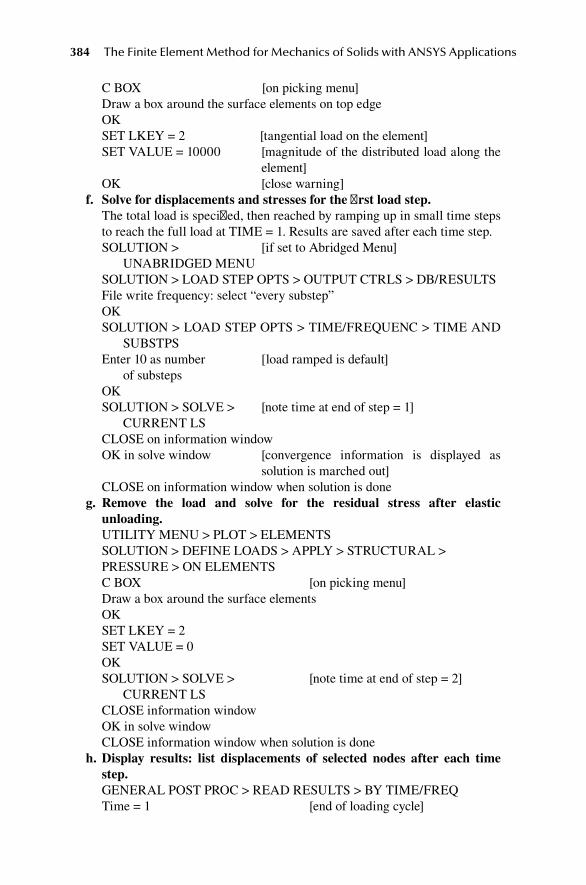
384 The Finite Element Method for Mechanics of Solids with ANSYS Applications
C BOX [on picking menu]Draw a box around the surface elements on top edgeOKSET LKEY = 2 [tangential load on the element]SET VALUE = 10000 [magnitude of the distributed load along the
element]OK [close warning]
f. Solve for displacements and stresses for the first load step. The total load is specified, then reached by ramping up in small time steps
to reach the full load at TIME = 1. Results are saved after each time step.SOLUTION > [if set to Abridged Menu]
UNABRIDGED MENUSOLUTION > LOAD STEP OPTS > OUTPUT CTRLS > DB/RESULTSFile write frequency: select “every substep”OKSOLUTION > LOAD STEP OPTS > TIME/FREQUENC > TIME AND
SUBSTPSEnter 10 as number [load ramped is default]
of substepsOKSOLUTION > SOLVE > [note time at end of step = 1]
CURRENT LSCLOSE on information windowOK in solve window [convergence information is displayed as
solution is marched out]CLOSE on information window when solution is done
g. Remove the load and solve for the residual stress after elastic unloading.UTILITY MENU > PLOT > ELEMENTSSOLUTION > DEFINE LOADS > APPLY > STRUCTURAL >PRESSURE > ON ELEMENTSC BOX [on picking menu]Draw a box around the surface elementsOKSET LKEY = 2 SET VALUE = 0 OK SOLUTION > SOLVE > [note time at end of step = 2]
CURRENT LSCLOSE information windowOK in solve windowCLOSE information window when solution is done
h. Display results: list displacements of selected nodes after each time step.GENERAL POST PROC > READ RESULTS > BY TIME/FREQTime = 1 [end of loading cycle]

ANSYS APDL Examples 385
OKGENERAL POST PROC > PLOT RESULTS > DEFORMED SHAPEC DEF & UNDEF OK and see deformed shapeUTILITY MENU > PLOT > ELEMENTSGENERAL POST PROC > QUERY RESULTS > SUBGRID SOLUTIONSTRESS SYOK [picking menu appears]Pick a node to see the value of SY [SY = 69,601 at lower-left corner]OKPLOT RESULTS > CONTOUR PLOT > NODAL SOLUTIONSTRESS > von Mises stressOK [note yielded region of S > 30,000]UTILITY MENU > PLOT > ELEMENTSTIME HIST POSTPROC [close information window FILE >
CLOSE]DEFINE VARIABLES [note that variable 1 is TIME,
which is a magnitude of load]ADD [click on the background to see the
body]Select Nodal DOF ResultOKPick upper right corner node (node 3)OKEnter name: U3Select Translation UXOK [variable 2 is UX at node 3]Close [you may have to move windows to
see the Defined Variables window]TIME HIST POSTPROC > LIST VARIABLESFor 1st variable to list: enter 2OK [list UX at corner for each time step]CLOSE
i. Plot stress distribution along a selected path after loading.Utility Menu > PLOT > ELEMENTSGENERAL POSTPROC > PATH OPERATIONS > DEFINE PATH > ON WORKING PLANEOKPick nodes at lower left then [zoom in as needed]
right corners
OKEnter path name: Baseenter nDiv = 50 [number of data points]OKFILE > CLOSE
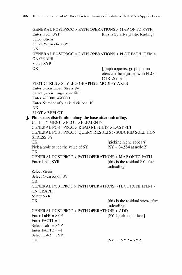
386 The Finite Element Method for Mechanics of Solids with ANSYS Applications
GENERAL POSTPROC > PATH OPERATIONS > MAP ONTO PATHEnter label: SYP [this is Sy after plastic loading]Select StressSelect Y-direction SYOKGENERAL POSTPROC > PATH OPERATIONS > PLOT PATH ITEM > ON GRAPHSelect SYPOK [graph appears, graph param-
eters can be adjusted with PLOT CTRLS menu]
PLOT CTRLS > STYLE > GRAPHS > MODIFY AXESEnter y-axis label: Stress SySelect y-axis range: specifiedEnter −70000, +70000Enter Number of y-axis divisions: 10OKPLOT > REPLOT
j. Plot stress distribution along the base after unloading.UTILITY MENU > PLOT > ELEMENTSGENERAL POST PROC > READ RESULTS > LAST SETGENERAL POST PROC > QUERY RESULTS > SUBGRID SOLUTIONSTRESS SYOK [picking menu appears]Pick a node to see the value of SY [SY = 34,584 at node 2]OKGENERAL POSTPROC > PATH OPERATIONS > MAP ONTO PATHEnter label: SYR [this is the residual SY after
unloading]Select StressSelect Y-direction SYOKGENERAL POSTPROC > PATH OPERATIONS > PLOT PATH ITEM > ON GRAPHSelect SYROK [this is the residual stress after
unloading]GENERAL POSTPROC > PATH OPERATIONS > ADDEnter LabR = SYE [SY for elastic unload]Enter FACT1 = 1Select Lab1 = SYPEnter FACT2 = −1Select Lab2 = SYROK [SYE = SYP − SYR]

ANSYS APDL Examples 387
GENERAL POSTPROC > PATH OPERATIONS > PLOT PATH ITEM > ON GRAPHSelect SYP, SYR, and SYEOK
15.14 vIScoelaStIcIty creep teSt
Viscoelastic materials are introduced. A step load is approximated by a very short time step. The Restart command is used to extend the solution.
This is a solution of the creep test for the standard linear solid model in shear with elastic volume change (Equation 9.17). The model for shear is as shown in Figure 15.12. In nondimensional units: μ1 = μ2 = η = 100. G(0) = 100, G(∞) = 0.5, G1 = 50, τ1 = 0.5. The volume change is elastic with bulk modulus κ = 650/3. Thus, E0 = 260, ν0 = 0.3. One element in plane stress provides the exact spatial distribution since the strain and stress are uniform.
a. Activate ANSYS and set analysis type.See example 15.3.
b. Establish element type and material properties.PREPROCESSOR > ELEMENT TYPE > ADDADDStructural SolidC 8 node 183 [this is element Plane183]OK [plane stress is the default]CLOSEPREPROCESSOR > MATERIAL PROP > MATERIAL MODELSSTRUCTURAL LINEAR > ELASTIC > ISOTROPICEX = 260 [E(0)]
μ1
μ2
s
2e
2e1
2e2
s
η
fIgure 15.12 Viscoelastic model for shear.
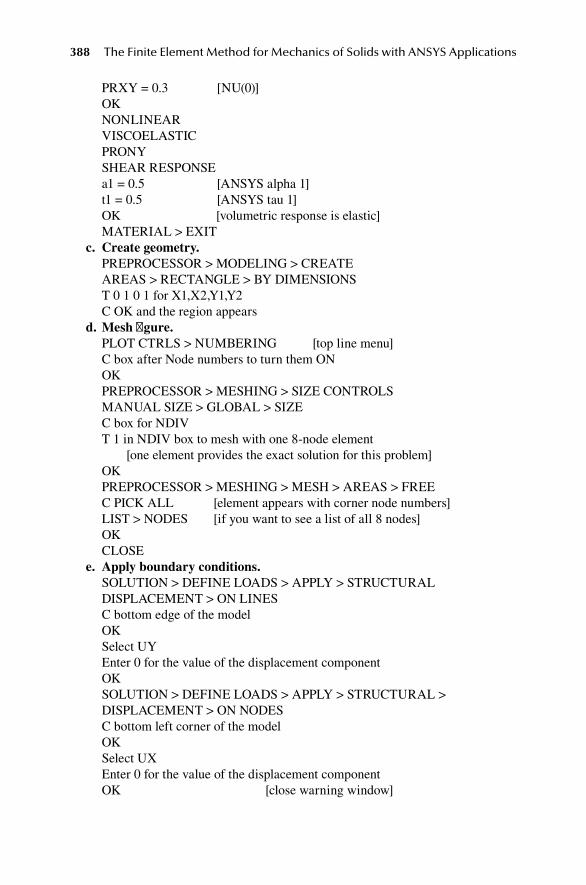
388 The Finite Element Method for Mechanics of Solids with ANSYS Applications
PRXY = 0.3 [NU(0)]OKNONLINEARVISCOELASTICPRONYSHEAR RESPONSEa1 = 0.5 [ANSYS alpha 1]t1 = 0.5 [ANSYS tau 1]OK [volumetric response is elastic]MATERIAL > EXIT
c. Create geometry.PREPROCESSOR > MODELING > CREATEAREAS > RECTANGLE > BY DIMENSIONST 0 1 0 1 for X1,X2,Y1,Y2C OK and the region appears
d. Mesh figure.PLOT CTRLS > NUMBERING [top line menu]C box after Node numbers to turn them ONOKPREPROCESSOR > MESHING > SIZE CONTROLSMANUAL SIZE > GLOBAL > SIZEC box for NDIVT 1 in NDIV box to mesh with one 8-node element [one element provides the exact solution for this problem]OKPREPROCESSOR > MESHING > MESH > AREAS > FREEC PICK ALL [element appears with corner node numbers]LIST > NODES [if you want to see a list of all 8 nodes]OKCLOSE
e. Apply boundary conditions.SOLUTION > DEFINE LOADS > APPLY > STRUCTURALDISPLACEMENT > ON LINESC bottom edge of the modelOKSelect UYEnter 0 for the value of the displacement componentOKSOLUTION > DEFINE LOADS > APPLY > STRUCTURAL > DISPLACEMENT > ON NODESC bottom left corner of the modelOKSelect UXEnter 0 for the value of the displacement componentOK [close warning window]
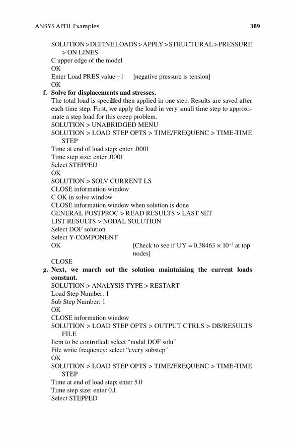
ANSYS APDL Examples 389
SOLUTION > DEFINE LOADS > APPLY > STRUCTURAL > PRESSURE > ON LINES
C upper edge of the modelOKEnter Load PRES value −1 [negative pressure is tension]OK
f. Solve for displacements and stresses. The total load is specified then applied in one step. Results are saved after
each time step. First, we apply the load in very small time step to approxi-mate a step load for this creep problem.SOLUTION > UNABRIDGED MENUSOLUTION > LOAD STEP OPTS > TIME/FREQUENC > TIME-TIME
STEPTime at end of load step: enter .0001Time step size: enter .0001Select STEPPEDOKSOLUTION > SOLV CURRENT LSCLOSE information windowC OK in solve windowCLOSE information window when solution is doneGENERAL POSTPROC > READ RESULTS > LAST SETLIST RESULTS > NODAL SOLUTIONSelect DOF solutionSelect Y-COMPONENTOK [Check to see if UY = 0.38463 × 10⁻² at top nodes]CLOSE
g. Next, we march out the solution maintaining the current loads constant.SOLUTION > ANALYSIS TYPE > RESTARTLoad Step Number: 1Sub Step Number: 1OKCLOSE information windowSOLUTION > LOAD STEP OPTS > OUTPUT CTRLS > DB/RESULTS
FILEItem to be controlled: select “nodal DOF solu”File write frequency: select “every substep”OKSOLUTION > LOAD STEP OPTS > TIME/FREQUENC > TIME-TIME
STEPTime at end of load step: enter 5.0Time step size: enter 0.1Select STEPPED

390 The Finite Element Method for Mechanics of Solids with ANSYS Applications
DELTIM minimum = 0.01DELTIM maximum = 0.1OKSOLUTION > SOLV CURRENT LSOK [close warning] [convergence information is displayed as solution is marched out]CLOSE information window when solution is done
h. Display results: list displacements of selected nodes after each time step.GENERAL POST PROC > READ RESULTS > LAST SETGENERAL POST PROC > PLOT RESULTS > DEFORMED SHAPEC DEF & UNDEF C OK and see deformed shapeTIME HIST POSTPROC [close information window]DEFINE VARIABLES [new window appears showing variable 1 is
the time]AddSelect Nodal DOF ResultOKPick corner node 6 [move window to see model]OKEnter name: DISPSelect Translation UY [variable 2 is UY]OKClose information windowTIME HIST POSTPROC > LIST VARIABLESFor 1st variable to list: enter 2OK [list UY at corner for each time step, UY =
0.0060546 at t = 5]FILE > PRINT [if desired]CLOSE
i. Plot results: plot the displacement at each time.Utility Menu: PLOT CTRLS > STYLE > GRAPHS > MODIFY AXESEnter x-axis label: TIMEEnter y-axis label: DISPSELECT: SPECIFIED Y-RANGEENTER Y-RANGE OF 0 TO 0.01OKTIME HIST POSTPROC > SETTINGS > GRAPHx-Axis variable: select Single VariableSingle variable: enter 1 [time on x-axis]OKTIME HIST POSTPROC > GRAPH VARIABLESFor 1st variable, enter 2 [displacement on y-axis]OK

ANSYS APDL Examples 391
15.15 vIScoelaStIcIty exaMple
This is a solution of the plane strain problem solved in Section 9.1.2 that is diagrammed in Figure 15.13. Material properties are as in Section 15.14, and the constant load is σ = 1. In nondimensional units: μ1 = μ2 = η =100. G(0) = 100, G(∞) = 0.5, G1 = 50, τ1 = 0.5. The volume change is elastic with bulk modulus κ = 650/3. Thus, E0 = 260, ν0 = 0.3. Support conditions are added to prevent rigid displacement without con-stricting the model.
a. Activate ANSYS and set analysis type.See example 15.3.
b. Establish element type and material properties.PREPROCESSOR > ELEMENT TYPE > ADDADDStructural SolidC 8 node 183 [this is element Plane183]OKOPTIONSSelect K3 = plane strainOKCLOSEPREPROCESSOR > MATERIAL PROP > MATERIAL MODELSSTRUCTURAL LINEAR > ELASTIC > ISOTROPICEX = 260 [E(0)]PRXY = 0.3 [NU(0)]OKNONLINEARVISCOELASTIC
1
1
y
x
σ
fIgure 15.13 Viscoelastic: plane strain.
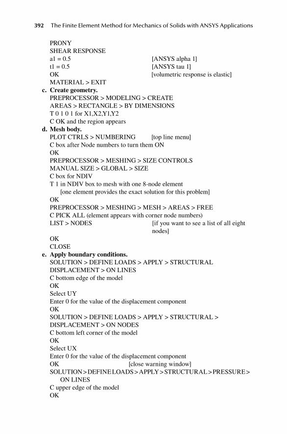
392 The Finite Element Method for Mechanics of Solids with ANSYS Applications
PRONYSHEAR RESPONSEa1 = 0.5 [ANSYS alpha 1]t1 = 0.5 [ANSYS tau 1]OK [volumetric response is elastic]MATERIAL > EXIT
c. Create geometry.PREPROCESSOR > MODELING > CREATEAREAS > RECTANGLE > BY DIMENSIONST 0 1 0 1 for X1,X2,Y1,Y2C OK and the region appears
d. Mesh body.PLOT CTRLS > NUMBERING [top line menu]C box after Node numbers to turn them ONOKPREPROCESSOR > MESHING > SIZE CONTROLSMANUAL SIZE > GLOBAL > SIZEC box for NDIVT 1 in NDIV box to mesh with one 8-node element [one element provides the exact solution for this problem]OKPREPROCESSOR > MESHING > MESH > AREAS > FREEC PICK ALL (element appears with corner node numbers)LIST > NODES [if you want to see a list of all eight
nodes]OKCLOSE
e. Apply boundary conditions.SOLUTION > DEFINE LOADS > APPLY > STRUCTURALDISPLACEMENT > ON LINESC bottom edge of the modelOKSelect UYEnter 0 for the value of the displacement componentOKSOLUTION > DEFINE LOADS > APPLY > STRUCTURAL > DISPLACEMENT > ON NODESC bottom left corner of the modelOKSelect UXEnter 0 for the value of the displacement componentOK [close warning window]SOLUTION > DEFINE LOADS > APPLY > STRUCTURAL > PRESSURE >
ON LINESC upper edge of the modelOK
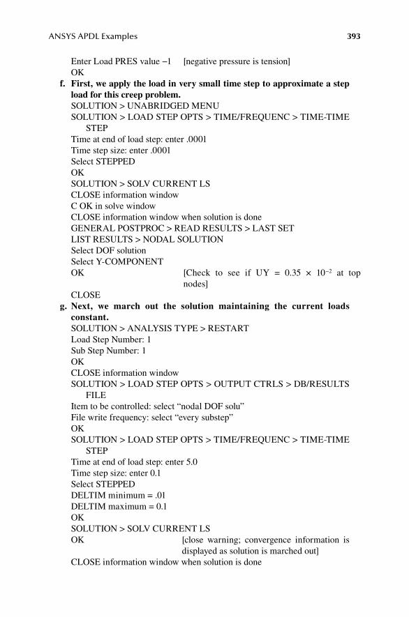
ANSYS APDL Examples 393
Enter Load PRES value −1 [negative pressure is tension]OK
f. First, we apply the load in very small time step to approximate a step load for this creep problem.SOLUTION > UNABRIDGED MENUSOLUTION > LOAD STEP OPTS > TIME/FREQUENC > TIME-TIME
STEPTime at end of load step: enter .0001Time step size: enter .0001Select STEPPEDOKSOLUTION > SOLV CURRENT LSCLOSE information windowC OK in solve windowCLOSE information window when solution is doneGENERAL POSTPROC > READ RESULTS > LAST SETLIST RESULTS > NODAL SOLUTIONSelect DOF solutionSelect Y-COMPONENTOK [Check to see if UY = 0.35 × 10⁻² at top
nodes]CLOSE
g. Next, we march out the solution maintaining the current loads constant.SOLUTION > ANALYSIS TYPE > RESTARTLoad Step Number: 1Sub Step Number: 1OKCLOSE information windowSOLUTION > LOAD STEP OPTS > OUTPUT CTRLS > DB/RESULTS
FILEItem to be controlled: select “nodal DOF solu”File write frequency: select “every substep”OKSOLUTION > LOAD STEP OPTS > TIME/FREQUENC > TIME-TIME
STEPTime at end of load step: enter 5.0Time step size: enter 0.1Select STEPPEDDELTIM minimum = .01DELTIM maximum = 0.1OKSOLUTION > SOLV CURRENT LSOK [close warning; convergence information is
displayed as solution is marched out]CLOSE information window when solution is done

394 The Finite Element Method for Mechanics of Solids with ANSYS Applications
h. Display results: list displacements of selected nodes after each time step.GENERAL POST PROC > READ RESULTS > LAST SETGENERAL POST PROC > PLOT RESULTS > DEFORMED SHAPEC DEF & UNDEF C OK and see deformed shapeTIME HIST POSTPROC [close information window]DEFINE VARIABLES [new window appears showing variable 1 is
the time]AddSelect Nodal DOF ResultOKPick corner node 6 [move window to see model]OKEnter name: DISPSelect Translation UY [variable 2 is UY]OKClose information windowTIME HIST POSTPROC > LIST VARIABLESFor 1st variable to list: enter 2OK [list UY at corner for each time step,
UY = 0.0060546 at t = 5]FILE > PRINT [if desired]CLOSE
i. Plot results: plot the displacement at each time.Utility Menu: PLOT CTRLS > STYLE > GRAPHS > MODIFY AXESEnter x-axis label: TIMEEnter y-axis label: DISPSELECT: SPECIFIED Y-RANGEENTER Y > RANGE OF 0 TO 0.01OKTIME HIST POSTPROC > SETTINGS > GRAPHx-Axis variable: select Single VariableSingle variable: enter 1 [time on x-axis]OKTIME HIST POSTPROC > GRAPH VARIABLESFor 1st variable, enter 2 [displacement on y-axis]OK
15.16 Mode ShapeS and frequencIeS of a rod
In this example, the determination of natural frequencies and mode shapes for the finite element model is introduced.
This is the solution to the problem analyzed in Section 10.4.2. The rod is mod-eled by two elements using lumped mass (Figure 15.14). The natural frequencies and

ANSYS APDL Examples 395
mode shapes for axial displacement are determined. In nondimensional units: A = 1, E = 1, ρ = 1, L = 1.
a. Activate ANSYS with structural preference.See example 15.3.
b. Choose elements and material. Use LINK1 element, enter the area in the Real Constants menu.
Linear, elastic, isotropic material model with E = 1, NUXY is not used. Density = 1. PREPROCESSOR > ELEMENT TYPE > ADD > ADDC 3D finit str 180OKCLOSEREAL CONSTANTS > ADD > ADDOKEnter AREA = 1OKCLOSEMATERIAL PROPERTIES > MATERIAL MODELSSTRUCTURALLINEARELASTICISOTROPICEnter EX = 1Enter PRXY = 0.3 [Poisson ratio, not used]OKDENSITYEnter 1OKMATERIAL > EXIT
c. Create nodes and elements.MODELING > CREATE > NODES > IN ACTIVE CSEnter NODE = 1, x,y,z = 0,0,0APPLYEnter 2 0.5 0 0APPLYEnter 3 1 0 0OK
0.50.5
1 2 31 2x
fIgure 15.14 Axial deformation of a rod.

396 The Finite Element Method for Mechanics of Solids with ANSYS Applications
ELEMENTS > AUTO NUMBERED > THRU NODESC on nodes 1 then 2 APPLYC on nodes 2 then 3OK
d. Apply loads and support conditions.SOLUTION > DEFINE LOADS > APPLY STRUCTURAL > DISPLACEMENT > ON NODESSELECT NODE 1 AND NODE 2APPLYSET UY = 0APPLYSELECT NODE 3OKSET ALL DOF = 0OK
e. Specify analysis type and options and solve.SOLUTION > ANALYSIS TYPE > NEW ANALYSISC MODALOKSOLUTION > ANALYSIS TYPE > ANALYSIS OPTIONSEnter 2 for No. of nodes to be extractedEnter 2 for No. of modes to expandSet LUMPM = YES [to use lumped mass]OK (Lanczos options window appears)OK to accept defaults [note: modes normalized to the mass
matrix]SOLUTION > SOLVE > CURRENT LSCLOSE (in Stat window)OK (To begin solution)CLOSE (solution is done)
f. List natural frequencies and mode shapes.GENERAL POSTPROC > RESULTS SUMMARY(list of natural frequencies in CPS appears)CLOSE windowGENERAL POSTPROC > READ RESULTS > FIRST SETLIST RESULTS > NODAL SOLUTION > DOF SOLUTIONSELECT X COMPONENTOK [see displacements for mode 1]CLOSEGENERAL POSTPROC > READ RESULTS > NEXT SETLIST RESULTS > NODAL SOLUTION > DOF SOLUTIONSELECT X COMPONENTOK [see displacements for mode 2]CLOSE
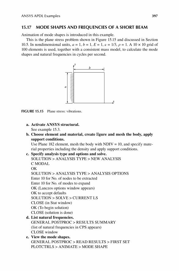
ANSYS APDL Examples 397
15.17 Mode ShapeS and frequencIeS of a Short BeaM
Animation of mode shapes is introduced in this example.This is the plane stress problem shown in Figure 15.15 and discussed in Section
10.5. In nondimensional units, a = 1, b = 1, E = 1, ν = 1/3, ρ = 1. A 10 × 10 grid of 100 elements is used, together with a consistent mass model, to calculate the mode shapes and natural frequencies in cycles per second.
a. Activate ANSYS structural.See example 15.3.
b. Choose element and material, create figure and mesh the body, apply support conditions.
Use Plane 182 element, mesh the body with NDIV = 10, and specify mate-rial properties including the density and apply support conditions.
c. Specify analysis type and options and solve.SOLUTION > ANALYSIS TYPE > NEW ANALYSISC MODALOKSOLUTION > ANALYSIS TYPE > ANALYSIS OPTIONSEnter 10 for No. of nodes to be extractedEnter 10 for No. of modes to expandOK (Lanczos options window appears)OK to accept defaultsSOLUTION > SOLVE > CURRENT LSCLOSE (in Stat window)OK (To begin solution)CLOSE (solution is done)
d. List natural frequencies.GENERAL POSTPROC > RESULTS SUMMARY(list of natural frequencies in CPS appears)CLOSE window
e. View the mode shapes.GENERAL POSTPROC > READ RESULTS > FIRST SETPLOTCTRLS > ANIMATE > MODE SHAPE
b
a
x
y
fIgure 15.15 Plane stress: vibrations.
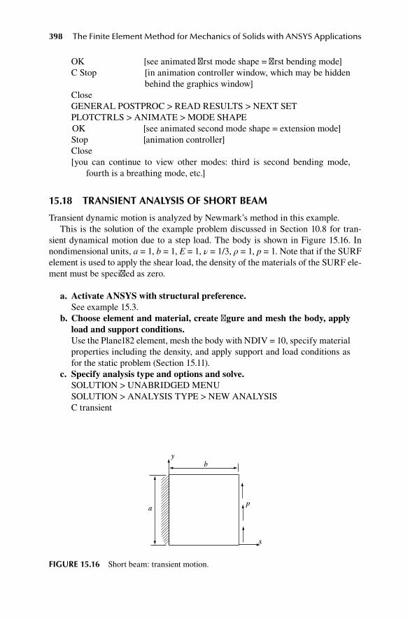
398 The Finite Element Method for Mechanics of Solids with ANSYS Applications
OK [see animated first mode shape = first bending mode]C Stop [in animation controller window, which may be hidden
behind the graphics window] CloseGENERAL POSTPROC > READ RESULTS > NEXT SETPLOTCTRLS > ANIMATE > MODE SHAPEOK [see animated second mode shape = extension mode]Stop [animation controller]Close[you can continue to view other modes: third is second bending mode,
fourth is a breathing mode, etc.]
15.18 tranSIent analySIS of Short BeaM
Transient dynamic motion is analyzed by Newmark’s method in this example.This is the solution of the example problem discussed in Section 10.8 for tran-
sient dynamical motion due to a step load. The body is shown in Figure 15.16. In nondimensional units, a = 1, b = 1, E = 1, ν = 1/3, ρ = 1, p = 1. Note that if the SURF element is used to apply the shear load, the density of the materials of the SURF ele-ment must be specified as zero.
a. Activate ANSYS with structural preference.See example 15.3.
b. Choose element and material, create figure and mesh the body, apply load and support conditions.
Use the Plane182 element, mesh the body with NDIV = 10, specify material properties including the density, and apply support and load conditions as for the static problem (Section 15.11).
c. Specify analysis type and options and solve.SOLUTION > UNABRIDGED MENUSOLUTION > ANALYSIS TYPE > NEW ANALYSISC transient
a
yb
x
p
fIgure 15.16 Short beam: transient motion.

ANSYS APDL Examples 399
OK [the options box appears]OK [i.e., use Full]SOLUTION > LOAD STEP OPTS > OUTPUT CTRLS > DB/RESULTS FILE [unabridged menu]Item to be controlled: select “nodal DOF solu”File write frequency: select “every substep”OKSOLUTION > LOAD STEP OPTS > TIME/FREQUENC > TIME/TIME
STEPTime at end of load step: enter 10Time step size: enter 0.1Select STEPPED [i.e., load is ramped up in first step]OKC SOLUTION > SOLV CURRENT LSC CLOSE on information windowC OK in solve windowC CLOSE on information window when solution is done
d. List results.TIME HIST POSTPROC Close information windowDEFINE VARIABLESADDSelect Nodal DOF ResultOKPick corner nodeOKEnter name: DISPLACEMENTSelect Translation Component UYOKCloseTIME HIST POSTPROC > LIST VARIABLESFor 1st variable to list: enter 2OKCLOSE
e. Plot results.Utility Menu: PLOT CTRLS > STYLE > GRAPHS > MODIFY AXESEnter x-axis label: TIMEEnter y-axis label: DISPLACEMENTSelect: specified x-rangeEnter x-range of 0 to 10Select: specified y-rangeEnter y-range of 0 to 15OKTIME HIST POSTPROC > GRAPH VARIABLESFor 1st variable, enter 2OK
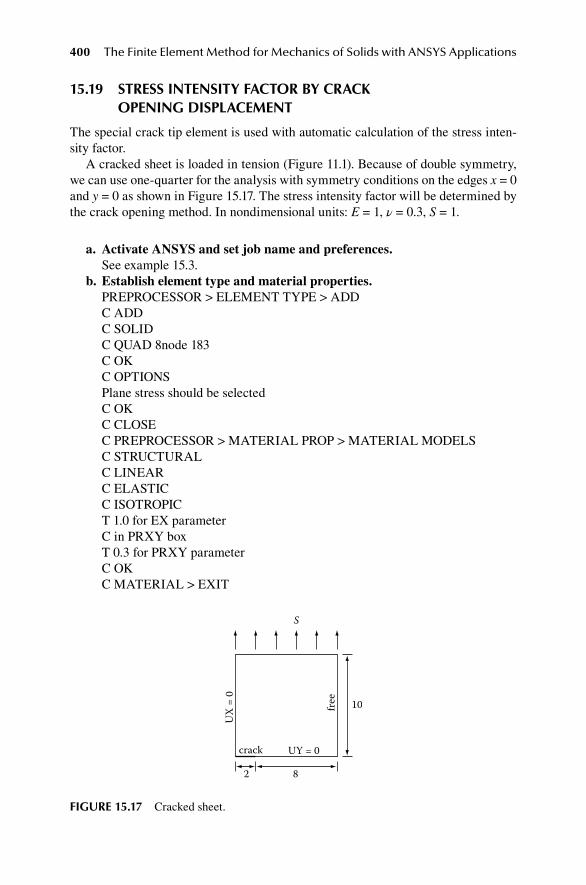
400 The Finite Element Method for Mechanics of Solids with ANSYS Applications
15.19 StreSS IntenSIty factor By crack openIng dISplaceMent
The special crack tip element is used with automatic calculation of the stress inten-sity factor.
A cracked sheet is loaded in tension (Figure 11.1). Because of double symmetry, we can use one-quarter for the analysis with symmetry conditions on the edges x = 0 and y = 0 as shown in Figure 15.17. The stress intensity factor will be determined by the crack opening method. In nondimensional units: E = 1, ν = 0.3, S = 1.
a. Activate ANSYS and set job name and preferences.See example 15.3.
b. Establish element type and material properties.PREPROCESSOR > ELEMENT TYPE > ADDC ADDC SOLIDC QUAD 8node 183C OKC OPTIONSPlane stress should be selectedC OKC CLOSE C PREPROCESSOR > MATERIAL PROP > MATERIAL MODELSC STRUCTURALC LINEARC ELASTICC ISOTROPICT 1.0 for EX parameterC in PRXY boxT 0.3 for PRXY parameterC OKC MATERIAL > EXIT
UX
= 0
crack UY = 0
82
free 10
S
fIgure 15.17 Cracked sheet.

ANSYS APDL Examples 401
c. Establish geometry and mesh the object. The upper right quarter of the cracked sheet is used. The origin as a
KEYPOINT is placed at the crack tip by using two rectangles and then combining them into one material body. The origin must be at the crack tip.C PREPROCESSOR > MODELING > CREATE > AREAS >C RECTANGLE > BY DIMENSIONST −2 0 0 10 for X1,X2,Y1,Y2 [note the minus sign]C APPLY and the first rectangle appearsT 0 8 0 10 for X1,X2,Y1,Y2C OK and the second rectangle appears [this ensures a keypoint at
the origin]PLOT CTRLS > NUMBERINGC box after Keypoint Numbers to turn them ONC box after Line Numbers to turn them ONC box after Area Numbers to turn them ONC box after Node numbers to turn them ONC OK (see all features numbered)C PREPROCESSOR > MODELING > OPERATE > BOOLEANS > ADD
> AREASC PICK ALL [this combines the two areas
into one area A3]C PREPROCESSOR > MESHING > SIZE CONTROLSC CONCENTRATE KPs > CREATEPICK crack tip at the originC OK (menu appears)Enter .25 for radius of first row of elementsEnter 1 for ratio of second row to firstEnter 6 for no. of elements around circum.Select SKEWED 1/4 PT from menu for KCTIPC OKC PREPROCESSOR > MESHING > MESH > AREAS > FREEC PICK ALL [close warning message]
d. Apply boundary conditions and solve for displacements and stresses.PLOT > LINESSOLUTION > DEFINE LOADS > APPLY > STRUCTURAL >
DISPLACEMENT > ON LINESC bottom right edge of the model (L9)C APPLYC UYEnter 0 for the value of the displacement componentsC APPLYC left edge of the model (L4)C OKC UX

402 The Finite Element Method for Mechanics of Solids with ANSYS Applications
Enter 0 for the value of the displacement components (Symmetry Condition)C OKC SOLUTION > DEFINE LOADS > APPLY > STRUCTURAL >
PRESSURE > ON LINESC top edge of both of the original two elements (L3 and L10)C OKEnter −1 for Load Pressure value [negative for tension]C OK C SOLUTION > SOLV CURRENT LSC CLOSE on information windowC OK in SOLVE windowC YES in warning windowCLOSE on information that solution is complete
e. Display results and calculate stress intensity factor. The active origin must be at the crack tip and a path of three nodes for cal-
culation of K must be defined.C GENERAL POST PROC > PLOT RESULTS > DEFORMED SHAPEC OK and see deformed shapeC UTILITY MENU > PLOT CTRLS > PAN,ZOOM,ROTATE Use circle and arrows to zoom in on crack tip regionC GENERAL POSTPROC > PATH OPERATIONS > DEFINE PATH >
BY NODESPICK crack tip and next two nodes on the crack surface (1, 61, 59) C OKEnter CRACK for path name.C OKC CLOSE listC GENERAL POST PROC > NODAL CALCS > STRESS INT FACTRSelect PLANE STRESS from the menu for KPLANSelect HALF-SYMM B.C. from the menu for KCSYMC OK produces listing showing KI = 2.6478CLOSE
15.20 StreSS IntenSIty factor By J-Integral
The Select command and use of the Command Line for typed commands are introduced.
A cracked sheet is loaded in tension (Figure 11.1). Because of double symmetry, we can use one-quarter for the analysis with symmetry conditions on the edges x = 0 and y = 0 as shown in Figure 15.17. The stress intensity factor will be determined by the J-integral method. In nondimensional units: E = 1, ν = 0.3, S = 1. The GUI is not available for the J-integral. The commands must be entered manually on the Command Line.
a. Activate ANSYS and set job name and preferences.See example 15.3.
b. Establish element type and material properties.

ANSYS APDL Examples 403
PREPROCESSOR > ELEMENT TYPE > ADDC ADDC SOLIDC QUAD 8node 183C OKC CLOSE C PREPROCESSOR > MATERIAL PROP > MATERIAL MODELSC STRUCTURALC LINEARC ELASTICC ISOTROPICT 1.0 for EX parameterC in PRXY boxT 0.3 for PRXY parameterC OKC MATERIAL > EXIT
c. Establish geometry and mesh the object. The upper right quarter of the cracked sheet is used. The origin as a KEYPOINT
is placed at the crack tip by using two rectangles and then combining them into one material body. The origin must be at the crack tip.C PREPROCESSOR > MODELING > CREATE > AREAS >RECTANGLE > BY DIMENSIONST −2 0 for X1,X2 and 0 10 for Y1,Y2 [note the minus sign]C APPLY and the first rectangle appearsT 0 8 for X1,X2 and 0 10 for Y1,Y2 C OK and the second rectangle appearsC PLOT CTRLS > NUMBERINGC box after Keypoint Numbers to turn them ONC box after Line Numbers to turn them ONC box after Area Numbers to turn them ONC box after Node numbers to turn them ONC OK (see all features numbered)C PREPROCESSOR > MODELING > OPERATE > BOOLEANS >
ADD > AREASC PICK ALL (this combines the two areas into one area A3)C PREPROCESSOR > MESHING > SIZE CONTROLSC CONCENTRATE KPs > CREATEPICK crack tip at the originC OK (menu appears)Enter .25 for radius of first row of elementsEnter 1 for ratio of second row to firstEnter 6 for no. of elements around circum.Select SKEWED 1/4 PT from menu for KCTIPOKC PREPROCESSOR > MESHING > MESH > AREAS > FREEC PICK ALL [close warning message]

404 The Finite Element Method for Mechanics of Solids with ANSYS Applications
d. Apply boundary conditions.C PLOT > LINESC LOADS > DEFINE LOADS > APPLY > STRUCTURAL >
DISPLACEMENT >ON LINESC bottom right edge of the model (L9)C APPLYC UYEnter 0 for the value of the displacement componentsC APPLYC left edge of the model (L4)C OKC UXOKC APPLY > STRUCTURAL > PRESSURE > ON LINESC top edge of both of the original two elements (L3 and L10)C OKEnter −1 for Load Pressure value [negative for tension]C OK
e. Create J-integral parameters.C PLOT > ELEMENTS [Utility menu]C SECLECT > ENTITIES [nodes by num/pick selected]C OKPick node at origin [zoom in to be sure you pick the
origin]C OKC SELECT > COMP/ASSEMBLY > CREATE COMPONENTEnter CRACK1 for CnameC OKC SELECT > EVERYTHING[type the following commands on the command line followed by ENTER]OUTRES,CINT,ALL [output J-integral results]CINT,NEW,1 [new contour integral with ID = 1]CINT,NAME,CRACK1 [node for path 1]CINT,NCON,3 [do for three contours]CINT,SYMM,ON [symmetric about crack line]CINT,NORM,0,2 [crack normal is y-axis]CINT,LIST [lists parameters in Output
Window]f. Solve equations.
C SOLUTION > SOLV CURRENT LSC CLOSE on information windowC OK in SOLVE windowC YES in warning window C CLOSE on information window that solution is complete
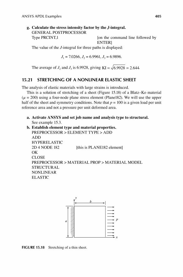
ANSYS APDL Examples 405
g. Calculate the stress intensity factor by the J-integral.GENERAL POSTPROCESSORType PRCINT,1 [on the command line followed by
ENTER]The value of the J-integral for three paths is displayed:
J1 = 7.0266, J2 = 6.9961, J3 = 6.9896.
The average of J2 and J3 is 6.9928, giving KI = =6 9928 2 644. . .
15.21 StretchIng of a nonlInear elaStIc Sheet
The analysis of elastic materials with large strains is introduced.This is a solution of stretching of a sheet (Figure 15.18) of a Blatz–Ko material
(μ = 200) using a four-node plane stress element (Plane182). We will use the upper half of the sheet and symmetry conditions. Note that p = 100 is a given load per unit reference area and not a pressure per unit deformed area.
a. Activate ANSYS and set job name and analysis type to structural.See example 15.3.
b. Establish element type and material properties.PREPROCESSOR > ELEMENT TYPE > ADDADDHYPERELASTIC2D 4 NODE 182 [this is PLANE182 element]OKCLOSEPREPROCESSOR > MATERIAL PROP > MATERIAL MODELSTRUCTURALNONLINEARELASTIC
by
a p
x
fIgure 15.18 Stretching of a thin sheet.
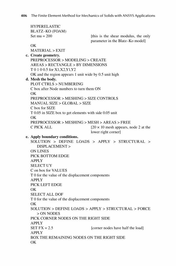
406 The Finite Element Method for Mechanics of Solids with ANSYS Applications
HYPERELASTICBLATZ–KO (FOAM)Set mu = 200 [this is the shear modulus, the only
parameter in the Blatz–Ko model]OKMATERIAL > EXIT
c. Create geometry.PREPROCESSOR > MODELING > CREATEAREAS > RECTANGLE > BY DIMENSIONST 0 1 0 0.5 for X1,X2,Y1,Y2OK and the region appears 1 unit wide by 0.5 unit high
d. Mesh the body.PLOT CTRLS > NUMBERINGC box after Node numbers to turn them ONOKPREPROCESSOR > MESHING > SIZE CONTROLSMANUAL SIZE > GLOBAL > SIZEC box for SIZET 0.05 in SIZE box to get elements with side 0.05 unitOKPREPROCESSOR > MESHING > MESH > AREAS > FREEC PICK ALL [20 × 10 mesh appears, node 2 at the
lower right corner]e. Apply boundary conditions.
SOLUTION > DEFINE LOADS > APPLY > STRUCTURAL > DISPLACEMENT >
ON LINESPICK BOTTOM EDGEAPPLYSELECT UYC on box for VALUEST 0 for the value of the displacement componentsAPPLYPICK LEFT EDGEOKSELECT ALL DOFT 0 for the value of the displacement componentsOKSOLUTION > DEFINE LOADS > APPLY > STRUCTURAL > FORCE
> ON NODESPICK CORNER NODES ON THE RIGHT SIDEAPPLYSET FX = 2.5 [corner nodes have half the load]APPLYBOX THE REMAINING NODES ON THE RIGHT SIDEOK

ANSYS APDL Examples 407
SET FX = 5 OK [Close Warning]
f. Solve for displacements and stresses. The total load is specified, then reached by ramping up in small time steps.
Results are saved after each time step.SOLUTION > UNABRIDGED MENUSOLUTION > ANALYSIS TYPE > ANALYSIS OPTIONS Set NLGEOM ON [this is for K0]Set Stress Stiff ON (SSTIF at [this is for K1]
the bottom)OKSOLUTION > LOAD STEP OPTS > OUTPUT CTRLS > DB/RESULTS
FILEFile write frequency: select “every substep”OKSOLUTION > LOAD STEP OPTS > TIME/FREQUENC > TIME/TIME
STEPTime at end of load step: enter 1Time step size: enter 0.1Select RAMPEDAutomatic time step: ONMinimum time step: enter 0.05Maximum time step: enter 0.1OKSOLUTION > SOLV > CURRENT LSCLOSE information windowOK in solve window(Convergence information is displayed as solution is marched out.)CLOSE information window when solution is done
g. Display results: list displacements of selected nodes after each time step.GENERAL POST PROC > PLOT RESULTS > DEFORMED SHAPEDEF & UNDEFOK and see deformed shapeGENERAL POST PROC > LIST RESULTSNODAL SOLUTIONDOF SOLUTION > X-ComponentOK [you should have UX = 0.4339 at
node 2]CLOSEGENERAL POST PROC > LIST RESULTSNODAL SOLUTIONSTRESS > X-COMPONENTOK [you should have SX = 120.19 at
node 2; this is the true stress T11]CLOSE
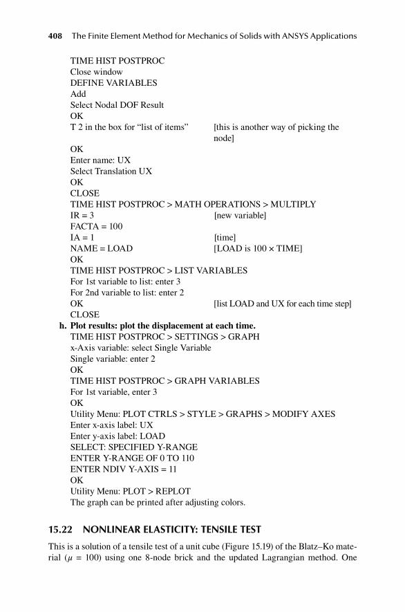
408 The Finite Element Method for Mechanics of Solids with ANSYS Applications
TIME HIST POSTPROC Close windowDEFINE VARIABLESAddSelect Nodal DOF ResultOKT 2 in the box for “list of items” [this is another way of picking the
node]OKEnter name: UXSelect Translation UXOKCLOSETIME HIST POSTPROC > MATH OPERATIONS > MULTIPLYIR = 3 [new variable]FACTA = 100IA = 1 [time]NAME = LOAD [LOAD is 100 × TIME]OKTIME HIST POSTPROC > LIST VARIABLESFor 1st variable to list: enter 3For 2nd variable to list: enter 2OK [list LOAD and UX for each time step]CLOSE
h. Plot results: plot the displacement at each time.TIME HIST POSTPROC > SETTINGS > GRAPHx-Axis variable: select Single VariableSingle variable: enter 2OKTIME HIST POSTPROC > GRAPH VARIABLESFor 1st variable, enter 3OKUtility Menu: PLOT CTRLS > STYLE > GRAPHS > MODIFY AXESEnter x-axis label: UXEnter y-axis label: LOADSELECT: SPECIFIED Y-RANGEENTER Y-RANGE OF 0 TO 110ENTER NDIV Y-AXIS = 11OKUtility Menu: PLOT > REPLOTThe graph can be printed after adjusting colors.
15.22 nonlInear elaStIcIty: tenSIle teSt
This is a solution of a tensile test of a unit cube (Figure 15.19) of the Blatz–Ko mate-rial (μ = 100) using one 8-node brick and the updated Lagrangian method. One

ANSYS APDL Examples 409
element is an exact model of the tensile test. The axial load is ramped up to P11 = 40. Minimum supports are imposed to prevent rigid displacement.
a. Activate ANSYS and set analysis type to structural.See example 15.3.
b. Establish element type and material properties.PREPROCESSOR > ELEMENT TYPE > ADDADDHYPERELASTICC 3D 8 NODE 185 [this is SOLID185 element]OKCLOSEPREPROCESSOR > MATERIAL PROP > MATERIAL MODELSTRUCTURALNONLINEARELASTICHYPERELASTICBLATZ–KO (FOAM)Set mu = 100 [this is the shear modulus, the only parameter in the
Blatz–Ko model]OKMATERIAL > EXIT
c. Create figure.PREPROCESSOR > MODELING > CREATE > VOLUMES > BLOCKBY DIMENSIONST 0 1 0 1 0 1 for X1,X2,Y1,Y2, Z1,Z2C OK and the region appears showing the x–y plane
d. Mesh body.PLOT CTRLS > NUMBERINGC box after Node numbers to turn them ONC OKPREPROCESSOR > MESHING > MESH TOOLC SIZE CONTROLS: GLOBL > SETC box for NDIVT 1 in NDIV box [one element is exact for the uniform extension]C OK
103
10
1010
465
UX = UY = UZ = 0 x2z
y
7UX = UZ = 0 1
UX = UY = 0
8UX = 0
fIgure 15.19 3D Tensile test.

410 The Finite Element Method for Mechanics of Solids with ANSYS Applications
C SHAPE: HEX [this forces a brick instead of the default tetrahedron]C MESHC PICK ALL [node numbers appear]C CLOSE [Mesh Tool]
e. Apply boundary conditions. First, rotate the element so that you can see the base (x = 0) with nodes 1-2-
5-8. This can be done in the dynamic model mode, which is interactive: on the right-hand side is a menu with 3D pictures of a block. Click on the but-ton at the end of the list that shows two elements (Dynamic Model Mode). The cursor changes to a rotation symbol. Hold down the right mouse button to rotate the element interactively until you can see the face 1-2-5-8.SOLUTION > DEFINE LOADS > APPLY > STRUCTURAL >
DISPLACEMENT > ON NODESC on node 2 (at the origin)APPLYC ALL DOFC on box for VALUEST 0 for the value of the displacement componentsAPPLYREPEAT THIS PROCESS TO SET UX AND UZ TO ZERO AT NODE 1REPEAT THIS PROCESS TO SET UX AND UY TO ZERO AT NODE 5REPEAT THIS PROCESS TO SET UX TO ZERO AT NODE 8[This prevents rigid body motion and keeps the base in the Y–Z plane, but
allows contraction.]ROTATE THE ELEMENT so that you can see the face x = 1 with nodes
3-4-6-7SOLUTION > DEFINE LOADS > APPLY > STRUCTURAL > FORCE
> ON NODESC ON EACH NODE 3-4-6-7OKSELECT FXT 10 for the VALUE of FX [this fixes the maximum load P11 = 40]C OK
f. Solve finite element equations.SOLUTION > UNABRIDGED MENUSOLUTION > ANALYSIS TYPE > ANALYSIS OPTIONSSet NLGEOM ON [this is for K0]Set Stress Stiff ON (SSTIF at the bottom) [this is for K1]OKSOLUTION > LOAD STEP OPTS > OUTPUT CTRLS > DB/RESULTS
FILEFile write frequency: select “every substep”OKSOLUTION > LOAD STEP OPTS > TIME/FREQUENC > TIME/TIME
STEP

ANSYS APDL Examples 411
Time at end of load step: enter 1Time step size: enter 0.1Select RAMPEDAutomatic time step: ONMinimum time step: enter 0.05Maximum time step: enter 0.1OKSOLUTION > SOLV CURRENT LSCLOSE information windowOK in solve window(Convergence information is displayed as solution is marched out.)CLOSE information window when solution is done
g. Display results: list displacements of selected nodes after each time step.GENERAL POST PROC > PLOT RESULTS > DEFORMED SHAPEDEF & UNDEF OK and see deformed shapeGENERAL POST PROC > LIST RESULTSNODAL SOLUTIONDOF SOLUTION > X-ComponentOK [you should have UX = 0.27104 at node 4]CLOSEGENERAL POST PROC > LIST RESULTSNODAL SOLUTIONSTRESS > X-COMPONENTOK [you should have SX = 45.096; this
is the true stress T11]CLOSETIME HIST POSTPROC CLOSE windowDEFINE VARIABLESADDSelect Nodal DOF ResultOKT 4 in the box for “list of items” [this is another way of picking the
node]OKEnter name: UXSelect Translation UXOKADDELEMENT RESULTSOKT 1 for the list of items [this is the element number]OKT 4 for the list of items [this is the node number for stress
output]

412 The Finite Element Method for Mechanics of Solids with ANSYS Applications
OKEnter name SX Select Stress Component SXOK CLOSE [variable 2 is UX and variable 3 is
SX] TIME HIST POSTPROC > LIST VARIABLESFor 1st variable to list: enter 3For 2nd variable to list: enter 2OK [lists SX and UX for each time
step]CLOSE
h. Plot results: plot the displacement at each time.TIME HIST POSTPROC > SETTINGS > GRAPHx-Axis variable: select Single VariableSingle variable: enter 2OKTIME HIST POSTPROC > GRAPH VARIABLESFor 1st variable, enter 3OKUtility Menu: PLOT CTRLS > STYLE > GRAPHS > MODIFY AXESEnter x-axis label: UXEnter y-axis label: SXSELECT: SPECIFIED Y-RANGEENTER Y-RANGE OF 0 TO 50SELECT: SPECIFIED X-RANGEENTER Y-RANGE OF 0 TO 0.3OKUtility Menu: PLOT > REPLOTThis graph can be printed for a report after adjusting colors
15.23 coluMn BucklIng
This example introduces the FILL command to generate intermediate nodes, the COPY ELEMENT command to proliferate elements, and the PRESTRESS com-mand to save the pre-buckling stress.
A column with one end fixed and the other free has an axial load P as shown in Figure 15.20. The cross section is 0.5 in.2: A = 0.25, I = 1/192, L = 100 in., E = 30 × 106 lb/in.2 The value of the buckling load is to be calculated. Ten elements of equal length are used.
L
PEIy
fIgure 15.20 Column buckling.
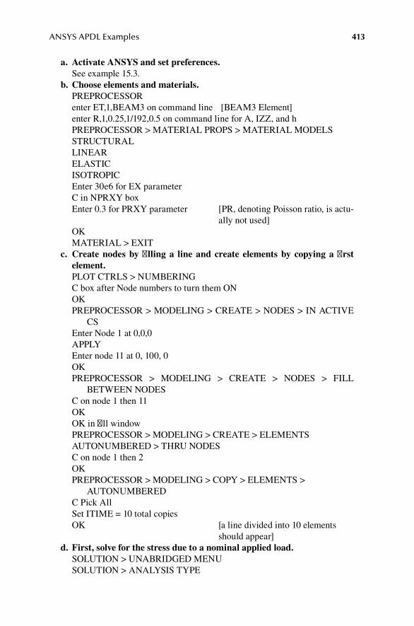
ANSYS APDL Examples 413
a. Activate ANSYS and set preferences.See example 15.3.
b. Choose elements and materials.PREPROCESSORenter ET,1,BEAM3 on command line [BEAM3 Element]enter R,1,0.25,1/192,0.5 on command line for A, IZZ, and hPREPROCESSOR > MATERIAL PROPS > MATERIAL MODELSSTRUCTURALLINEARELASTICISOTROPICEnter 30e6 for EX parameter C in NPRXY boxEnter 0.3 for PRXY parameter [PR, denoting Poisson ratio, is actu-
ally not used]OKMATERIAL > EXIT
c. Create nodes by filling a line and create elements by copying a first element.PLOT CTRLS > NUMBERING C box after Node numbers to turn them ONOKPREPROCESSOR > MODELING > CREATE > NODES > IN ACTIVE
CSEnter Node 1 at 0,0,0APPLYEnter node 11 at 0, 100, 0OKPREPROCESSOR > MODELING > CREATE > NODES > FILL
BETWEEN NODESC on node 1 then 11OKOK in fill windowPREPROCESSOR > MODELING > CREATE > ELEMENTSAUTONUMBERED > THRU NODESC on node 1 then 2OKPREPROCESSOR > MODELING > COPY > ELEMENTS >
AUTONUMBEREDC Pick AllSet ITIME = 10 total copiesOK [a line divided into 10 elements
should appear]d. First, solve for the stress due to a nominal applied load.
SOLUTION > UNABRIDGED MENUSOLUTION > ANALYSIS TYPE

414 The Finite Element Method for Mechanics of Solids with ANSYS Applications
ANALYSIS OPTIONS > PRESTRESS ON [near the bottom] OK [this saves the stress state for the
eigenvalue calculation]SOLUTION > DEFINE LOADS > APPLY > STRUCTURAL DISPLACEMENT > ON NODESC node 1OKC ALL DOF C on box for VALUEST 0 for the value of the displacements and rotationOK SOLUTION > DEFINE LOADS > APPLY > STRUCTURAL FORCE > ON NODESC node 11OKC FY C on VALUE boxT value for FY = −1 [negative for compressive force]OK [force shown on the node]SOLUTION > SOLVE > CURRENT LSCLOSE information window [check: Prestress Effects Calculated
is YES]C OK in solve windowCLOSE information window [solution is done]
e. Solve for the multiple of the applied load that produces a zero determi-nant for the total stiffness matrix.SOLUTION > ANALYSIS TYPE > NEW ANALYSISSelect EIGEN BUCKLINGOK [Close Warning If Any]SOLUTION > ANALYSIS OPTIONSEnter 1 mode to be extracted [NMODE]OK in options windowSOLUTION > SOLVE > CURRENT LSCLOSE information windowOK in solve windowCLOSE information window
f. Display results.GENERAL POST PROCESSOR > RESULTS SUMMARY[TIME/FREQ is the factor multiplying the nominal load to get the buckling
load, 38.553]CLOSEC GENERAL POST PROC > READ RESULTS > FIRST SETPLOT RESULTS > DEFORMED SHAPEC DEF & UNDEF C OK and see buckled mode shape

ANSYS APDL Examples 415
15.24 coluMn poSt-BucklIng
A column with one end fixed and the other free has an axial load P as shown in Figure 15.20. The cross section is 0.5 in.2: A = 0.25, I = 1/192, L = 100 in., E = 30 × 106 lb/in.2 The value of the buckling load has been calculated as Pcr = 38.553 lb. The post-buckling displacement is to be determined if the load is increased to P = 44. The column is placed so that the top is 1 in. out of alignment in order to simulate an imperfection.
a. Activate ANSYS, change job name and set preferences.See example 15.3.
b. Choose elements and materials.See section 15.23.
c. Create nodes by filling a line and create elements by copying a first element.PLOT CTRLS > NUMBERING C box after Node numbers to turn them ONOKPREPROCESSOR > MODELING > CREATE > NODES > IN ACTIVE
CSEnter Node 1 at 0,0,0APPLYEnter node 11 at 1, 100, 0 [note x = 1 off-set]OKFILL BETWEEN NODESC on node 1 then 11OKOK in fill windowPREPROCESSOR > MODELING > CREATE > ELEMENTSAUTONUMBERED > THRU NODESC on nodes 1 then 2OKPREPROCESSOR > MODELING > COPY > ELEMENTS >
AUTONUMBEREDC Pick AllSet ITIME = 10 total copiesOK
d. Apply boundary conditions.PREPROCESSOR > LOADS > DEFINE LOADS > APPLY >
STRUCTURAL DISPLACEMENT > ON NODESC node 1OKC ALL DOF C on box for VALUEST 0 for the value of the displacements and rotationOK
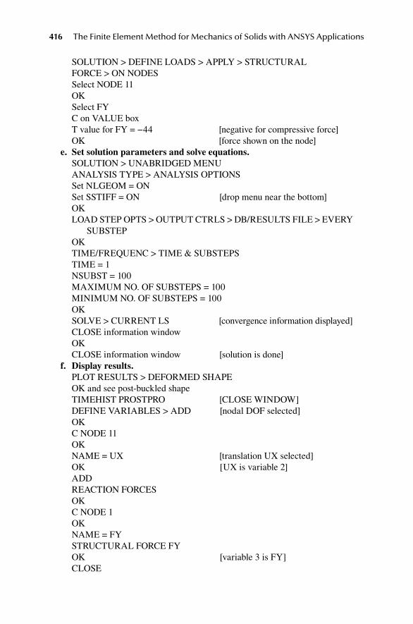
416 The Finite Element Method for Mechanics of Solids with ANSYS Applications
SOLUTION > DEFINE LOADS > APPLY > STRUCTURAL FORCE > ON NODESSelect NODE 11OKSelect FY C on VALUE boxT value for FY = −44 [negative for compressive force]OK [force shown on the node]
e. Set solution parameters and solve equations.SOLUTION > UNABRIDGED MENUANALYSIS TYPE > ANALYSIS OPTIONSSet NLGEOM = ONSet SSTIFF = ON [drop menu near the bottom]OKLOAD STEP OPTS > OUTPUT CTRLS > DB/RESULTS FILE > EVERY
SUBSTEPOKTIME/FREQUENC > TIME & SUBSTEPS TIME = 1NSUBST = 100MAXIMUM NO. OF SUBSTEPS = 100MINIMUM NO. OF SUBSTEPS = 100OKSOLVE > CURRENT LS [convergence information displayed]CLOSE information windowOKCLOSE information window [solution is done]
f. Display results.PLOT RESULTS > DEFORMED SHAPEOK and see post-buckled shapeTIMEHIST PROSTPRO [CLOSE WINDOW]DEFINE VARIABLES > ADD [nodal DOF selected]OKC NODE 11OKNAME = UX [translation UX selected]OK [UX is variable 2]ADDREACTION FORCESOKC NODE 1OKNAME = FYSTRUCTURAL FORCE FYOK [variable 3 is FY]CLOSE
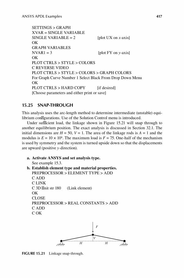
ANSYS APDL Examples 417
SETTINGS > GRAPHXVAR = SINGLE VARIABLESINGLE VARIABLE = 2 [plot UX on x-axis]OKGRAPH VARIABLESNVAR1 = 3 [plot FY on y-axis]OKPLOT CTRLS > STYLE > COLORS C REVERSE VIDEOPLOT CTRLS > STYLE > COLORS > GRAPH COLORSFor Graph Curve Number 1 Select Black From Drop Down MenuOK PLOT CTRLS > HARD COPY [if desired][Choose parameters and either print or save]
15.25 Snap-through
This analysis uses the arc-length method to determine intermediate (unstable) equi-librium configurations. Use of the Solution Control menu is introduced.
Under sufficient load, the linkage shown in Figure 15.21 will snap through to another equilibrium position. The exact analysis is discussed in Section 32.1. The initial dimensions are H = 50, V = 1. The area of the linkage rods is A = 1 and the modulus is E = 10 × 106. The maximum load is F = 75. One-half of the mechanism is used by symmetry and the system is turned upside down so that the displacements are upward (positive y-direction).
a. Activate ANSYS and set analysis type.See example 15.3.
b. Establish element type and material properties.PREPROCESSOR > ELEMENT TYPE > ADDC ADDC LINKC 3D finit str 180 (Link element)OKCLOSEPREPROCESSOR > REAL CONSTANTS > ADDC ADDC OK
F
HHV
fIgure 15.21 Linkage snap-through.

418 The Finite Element Method for Mechanics of Solids with ANSYS Applications
C in the AREA boxT 1.0 for areaC OKC CLOSEPREPROCESSOR > MATERIAL PROPS > MATERIAL MODELSC STRUCTURALC LINEARC ELASTICC ISOTROPICT 1e7 for EX parameterOK (PRXY is not used)MATERIAL > EXIT
c. Create a line and mesh it as one element.PREPROCESSOR > MODELING > CREATE > KEYPOINTS > IN
ACTIVE CSNPT = 1X,Y = 0,0C APPLYNPT = 2X,Y = 50, −1OKPREPROCESSOR > MODELING > CREATE > LINES > LINES >
STRAIGHT LINEPICK KP1PICK KP2OKPLOT CTRLS > NUMBERING [top line menu]C box after Node numbers to turn them ONOKPREPROCESSOR > MESHING > SIZE CONTROLSMANUAL SIZE > GLOBAL > SIZEC box for NDIVT 1 in NDIV box to mesh with one truss elementOKPREPROCESSOR > MESHING > MESH > LINESC PICK ALL [element appears with node and element
numbers]d. Apply boundary conditions.
SOLUTION > DEFINE LOADS > APPLY > STRUCTURALDISPLACEMENT > ON NODESPICK NODE 1OKC ALL DOFC on box for VALUEST 0 for the value of the displacement componentOK

ANSYS APDL Examples 419
SOLUTION > DEFINE LOADS > APPLY > STRUCTURAL > DISPLACEMENT > ON NODESPICK NODE 2OKSelect UX [be sure that only UX is highlighted]T 0 for the value of the displacement component [symmetry
condition]OK SOLUTION > DEFINE LOADS > APPLY > STRUCTURAL > FORCE
> ON NODESPICK NODE 2OKSELECT FYVALUE = 75 [this will be the maximum load]OK
e. Solve for displacements and stresses. The total load is specified and applied in one step. Results are saved after
each substep.SOLUTION > ANALYSIS TYPE > SOL’N CONTROLS > BASICSelect Analysis Option: Large Displacement Static [NLGEOM ON]Number of Substeps selectedEnter Number of substeps = 50Select Frequency: Write Every SubstepC ADVANCED NONLINEARC Activate Arc-Length MethodT Max Multiplier = +1T Min Multiplier = −1OKSOLUTION > SOLVE > CURRENT LSCLOSE blue information windowC OK in information window [“time” is actually the
load multiplier]CLOSE information window when solution is done
f. Display results: list displacements of selected nodes after each time step.GENERAL POST PROC > PLOT RESULTS > DEFORMED SHAPEC DEF & UNDEF C OK and see deformed shapeTIME HIST POSTPROC [close information
window]DEFINE VARIABLES [variable 1 labeled
time is actually the load multiplier]
Add Select Nodal DOF ResultOK

420 The Finite Element Method for Mechanics of Solids with ANSYS Applications
Pick node 2 [move window to see model]
OKEnter name: DISPLACEMENTSelect Translation UY [variable 2 is set to
UY]OKClose information windowTIME HIST POSTPROC > LIST VARIABLES [Time = Load
Multiplier]For NVAR2 enter 2 [displacement]OKCLOSE
g. Plot results: plot the displacement at each time.Utility Menu: PLOT CTRLS > STYLE > GRAPHS > MODIFY AXESEnter x-axis label: DISPLACEMENTEnter y-axis label: LOAD FACTORSELECT SPECIFIED X-RANGEENTER X-RANGE OF 0 TO 2.5SELECT: SPECIFIED Y-RANGEENTER Y-RANGE OF −1 TO +1OKTIME HIST POSTPROC > SETTINGS > GRAPHx-Axis variable: select Single VariableSingle variable: enter 2 [displacement on x-axis]OKTIME HIST POSTPROC > GRAPH VARIABLESFor 1st variable, enter 1 [load multiplier on y-axis]OK
15.26 plate BendIng exaMple
The Element Table is used to extract the moments and shears.This example is a solution of bending of a square plate by a uniform load. Two
opposite sides are simply supported with zero twisting moment and the other two opposite sides are simply supported with zero twisting rotation. One-quarter of the plate is modeled with symmetry conditions (Figure 15.22). In nondimensional units: a = b = 10, h = 1, ν = 0.3, D = 1, so that E = 10.92. This is a thick plate since a/h = 10.
a. Activate ANSYS and set job name and analysis type structural.See example 15.3.
b. Establish element type and material properties.PREPROCESSOR > ELEMENT TYPE > ADDADDSHELL
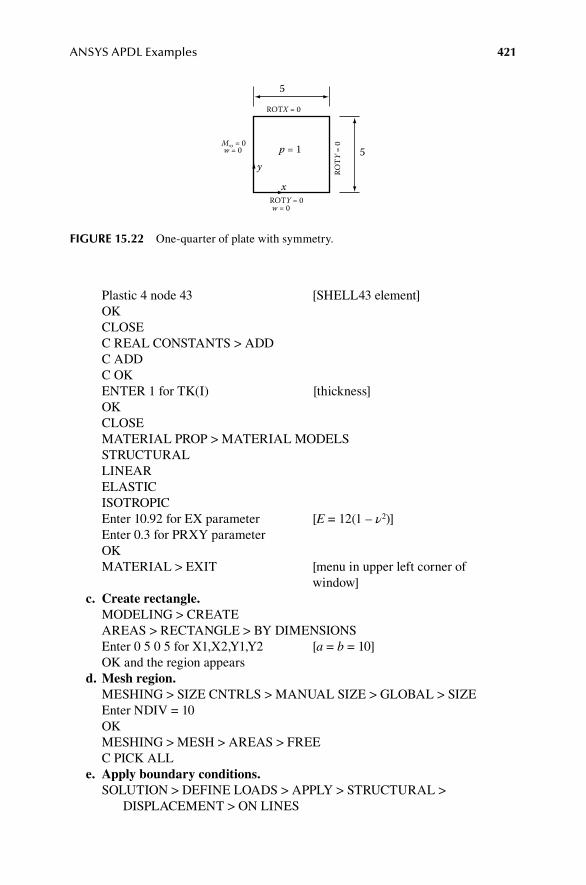
ANSYS APDL Examples 421
Plastic 4 node 43 [SHELL43 element]OKCLOSEC REAL CONSTANTS > ADDC ADDC OKENTER 1 for TK(I) [thickness]OKCLOSEMATERIAL PROP > MATERIAL MODELSSTRUCTURAL LINEARELASTICISOTROPICEnter 10.92 for EX parameter [E = 12(1 – ν2)]Enter 0.3 for PRXY parameter OKMATERIAL > EXIT [menu in upper left corner of
window]c. Create rectangle.
MODELING > CREATEAREAS > RECTANGLE > BY DIMENSIONSEnter 0 5 0 5 for X1,X2,Y1,Y2 [a = b = 10]OK and the region appears
d. Mesh region.MESHING > SIZE CNTRLS > MANUAL SIZE > GLOBAL > SIZEEnter NDIV = 10OKMESHING > MESH > AREAS > FREEC PICK ALL
e. Apply boundary conditions.SOLUTION > DEFINE LOADS > APPLY > STRUCTURAL > DISPLACEMENT > ON LINES
ROTX = 0
p = 1y
xROTY = 0w = 0
Mxy = 0w = 0
ROT
Y =
0
5
5
fIgure 15.22 One-quarter of plate with symmetry.
422 The Finite Element Method for Mechanics of Solids with ANSYS Applications
C bottom AND left edge of the modelAPPLYC UZ C on box for VALUEST 0 for the value of the displacement componentsAPPLY C bottom AND right edge of the modelAPPLYC ROTY APPLYC top edgeOKC ROTXOKDEFINE LOADS > APPLY > STRUCTURAL > PRESSURE > ON
AREASC PICK ALLEnter VALUE = 1 [default LKEY = 1]C OK [uniform load in positive z-direction]
f. Solve for displacements and stresses.SOLVE > CURRENT LSOKCLOSECLOSE
g. Display results: list displacements of selected nodes after each time step.PLOT CTRLS > NUMBERINGC NODE numbers ONSelect Elem/Attrib numbering = Element NumbersSelect /NUM = Numbers onlyOKGENERAL POST PROC > LIST RESULTS > NODAL SOLUTIONDOF SOLUTION > Z-COMPONENT OF DISPLACEMENT OK [w = 44.379 at the center]CLOSEELEMENT TABLE > DEFINE TABLE > ADDEnter Lab = MXC item by sequence numberEnter for SMISC, 4APPLYRepeat for MY 5, MXY 6, QX 7. and QY 8OKCLOSELIST ELEM TABLESELECT MX, MY, MXY, QX, QY

ANSYS APDL Examples 423
OK [see list of stress resultants at center of each element]
h. Graph results.PATH OPERATIONS > DEFINE PATH > BY NODESPick nodes along the base Y = 0 from the left to the centerOKEnter BASE for the nameOKCLOSEMAP ONTO PATHEnter LAB = QYC Elem Table ItemEnter for ETAB, QYOK [ANSYS extrapolates to the boundary]PLOT PATH ITEM>ON GRAPHSelect QYOKPLOT CTRLS > STYLE > GRAPHS > MODIFY AXESC Y-axis range specifiedEnter YMIN, YMAX as −5 to + 5OKPLOT > REPLOT
15.27 claMped plate
This is a solution of bending of a square plate by a uniform load. The edges of the plate are clamped (all DOFs are zero). The lateral load is uniformly distributed. Symmetry is not used. In nondimensional units: a = b = 20, h = 1, ν = 0.3, D = 100, so that E = 1092. This is a thick plate since a/h = 20.
a. Activate ANSYS and set job name and analysis type structural.See Example 15.3.
b. Establish element type and material properties.PREPROCESSOR > ELEMENT TYPE > ADDADDSHELLElastic 8 node 281 [SHELL281 element]OKCLOSEC REAL CONSTANTS > ADDC ADDC OKENTER 1 for TK(I) [thickness]OKCLOSE

424 The Finite Element Method for Mechanics of Solids with ANSYS Applications
MATERIAL PROP > MATERIAL MODELSSTRUCTURAL LINEARELASTICISOTROPIC Enter 1092 for EX parameter [D = 100]Enter 0.3 for PRXY parameter OKMATERIAL > EXIT
c. Create rectangle.MODELING > CREATEAREAS > RECTANGLE > BY DIMENSIONSEnter 0 20 0 20 for X1,X2,Y1,Y2 [a = b = 20]OK and the region appears
d. Mesh region.MESHING > SIZE CNTRLS > MANUAL SIZE > GLOBAL > SIZEEnter NDIV = 20OKMESHING > MESH > AREAS > FREEC PICK ALL
e. Apply boundary conditions.SOLUTION > DEFINE LOADS > APPLY > STRUCTURAL > DISPLACEMENT > ON LINESC all four edges OKC ALL DOFC on box for VALUEST 0 for the value of the displacement componentsOKDEFINE LOADS > APPLY > STRUCTURAL > PRESSURE > ON
AREASC PICK ALLEnter VALUE = 1 [default LKEY = 1]C OK [uniform load in the positive z-direction]
f. Solve for displacements and stresses.SOLVE > CURRENT LSOKCLOSECLOSE
g. View results.GENERASL POSTPROCQUERY RESULTSSUBGRID SOLUDOF SOLUTION > UZPick center nodeOK [see 2.1236, thin plate theory = 2.016]

ANSYS APDL Examples 425
15.28 gravIty load on a cylIndrIcal Shell
In this example, the command Select > Entities is used to select a set of noses. The use of stored parameters instead of directly entered data, cylindrical coordinates as the active coordinate system, and mapped meshing are introduced.
The cylindrical shell (Figure 15.23) is loaded by gravity in the y-direction. The curved shell is approximated by flat plate elements. The ends are supported by flex-ible membranes and the sides are free. E = 3 × 10⁶ lb/in.2, ν = 0, and the specific weight is 0.208 pci, r = 300 in., thickness = 3 in., length = 600 in. Double symmetry will be used.
a. Activate ANSYS and set analysis type.FILE > CHANGE JOBNAMET a job name [this is the internal job name, e.g., Shell]OKFILE > CHANGE TITLET a project name [this is the name on reports, e.g., Shell Roof]OKPREFERENCESC box before structuralOK
b. Establish element type and material properties.PREPROCESSOR > ELEMENT TYPE > ADDC ADDC SHELLC Elastic 4 node 181 [Shell181]OK
L
z
x
v = 0u = 0
v = 0u = 0
free
symsym
free
y y
x
r
40°
fIgure 15.23 Cylindrical shell.

426 The Finite Element Method for Mechanics of Solids with ANSYS Applications
CLOSEPREPROCESSOR > REAL CONSTANTS > ADDC ADDC OKTK(I) = 3 C OKC CLOSEPREPROCESSOR > MATERIAL PROPS > MATERIAL MODELSSTRUCTURALLINEARELASTICISOTROPICEX = 3e6 NUXY = 0.OK DENSITYDENS = .208OK MATERIAL > EXIT
c. Enter the value of some parameters for later use. The name of the parameter and its value or a formula is entered into the
selection box.UTILITY MENU > PARAMETRS > SCALAR PARAMETEREnter r = 300ACCEPTEnter z = 300 [length of one-half of shell]ACCEPTCLOSE
d. Change to cylindrical coordinates and create the surface. We are analyzing one-quarter of the shell and using symmetry conditions.
UTILITY MENU > WORK PLANE > CHANGE ACTIVE CS > GLOBAL CYLINDRICAL [cylindrical coordinates X → r, Y →
θ (in deg.)]PREPROCESSOR > MODELING > CREATE > KEYPOINTS > IN
ACTIVE CSNPT = 1X,Y,Z = r,50,0 [the values of parameter r will be used]C APPLYNPT = 2X,Y,Z = r,90,0C APPLYNPT = 3X,Y,Z = r,90,zC APPLYNPT = 4X,Y,Z = r,50,z
ANSYS APDL Examples 427
OKC ISOMETRIC VIEW [top icon on the right side menu]PREPROCESSOR > MODELING > CREATE AREAS > ARBITRARY > THROUGH KPsPICK KP1PICK KP2PICK KP3PICK KP4OK [area appears: this is a curved sur-
face in cylindrical coordinates]e. Mesh the surface.
PREPROCESSOR > MESHING > SIZE CONTROLSMANUAL SIZE > GLOBAL > SIZEC box for NDIVT 20 in NDIV box OKPREPROCESSOR > MESHING > MESH > AREASMAPPED > 3 OR 4 SIDEDC PICK ALL [20 × 20 mesh appears]
f. Apply boundary conditions using symmetry conditions.C TOP VIEW [right side menu]UTILITY MENU > SELECT > ENTITIESOK [to select nodes, picking menu
appears]C BOX Select nodes by drawing a box around the nodes on the left edge (global
X = 0) with mouse OKSOLUTION > DEFINE LOADS > APPLY > STRUCTURAL >
DISPLACEMENTSYMMETRY B.C. > ON NODES [menu appears]Norml = Y-axis [actually θ = 90° plane]KCN = 1 [global cylindrical coordinate
system]OK [support symbols appear]UTILITY MENU > SELECT > ENTITIESOK C BOX Select nodes by drawing a box around the nodes on the bottom edge
(Z = 300) OKSOLUTION > DEFINE LOADS > APPLY > STRUCTURAL >
DISPLACEMENTSYMMETRY B.C. > ON NODES Norml = Z-axis KCN = 1
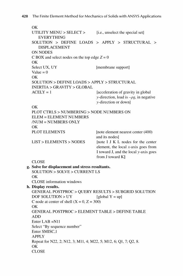
428 The Finite Element Method for Mechanics of Solids with ANSYS Applications
OKUTILITY MENU > SELECT > [i.e., unselect the special set]
EVERYTHINGSOLUTION > DEFINE LOADS > APPLY > STRUCTURAL >
DISPLACEMENTON NODESC BOX and select nodes on the top edge Z = 0OKSelect UX, UY [membrane support]Value = 0OKSOLUTION > DEFINE LOADS > APPLY > STRUCTURALINERTIA > GRAVITY > GLOBALACELY = 1 [acceleration of gravity in global
y-direction, load is –ρg, in negative y-direction or down]
OKPLOT CTRLS > NUMBERING > NODE NUMBERS ONELEM = ELEMENT NUMBERS /NUM = NUMBERS ONLY OKPLOT ELEMENTS [note element nearest center (400)
and its nodes]LIST > ELEMENTS > NODES [note I J K L nodes for the center
element, the local x-axis goes from I toward J, and the local y-axis goes from J toward K]
CLOSEg. Solve for displacement and stress resultants.
SOLUTION > SOLVE > CURRENT LSOKCLOSE information windows
h. Display results.GENERAL POSTPROC > QUERY RESULTS > SUBGRID SOLUTIONDOF SOLUTION > UY [global Y = up]C node at center of shell (X = 0, Z = 300)OK GENERAL POSTPROC > ELEMENT TABLE > DEFINE TABLEADDEnter LAB =N11Select “By sequence number”Enter SMISC,1APPLYRepeat for N22, 2; N12, 3; M11, 4; M22, 5; M12, 6; Q1, 7; Q2, 8.OKCLOSE

ANSYS APDL Examples 429
GENERAL POSTPROC > ELEMENT TABLE > LIST ELEM TABLESelect N11, N22, N12, M11, M22, M12Y, Q1, Q2 [values are at the
centroid]OKCLOSE
i. Plot results.GENERAL POSTPROC > PATH OPERATIONS > DEFINE PATH > BY
NODESSelect node 22 (z = 300, θ = 90) and then node 42 (z = 300, θ = 50).OKEnter path name Z = 300OKCLOSEGENERAL POSTPROC > PATH OPERATIONS > MAP ONTO PATHEnter LAB = UY [vertical displacement]Select UYOKGENERAL POSTPROC > PATH OPERATIONS > PLOT PATH ITEM >
ON GRAPHSelect UYOK [UY vs. arc length from the top]
15.29 plate BucklIng
A simply supported plate is loaded along one edge by in-plane loads (Figure 15.24). The buckling load is calculated. Use zero rotation about the normal to the edge for the simply supported condition. Use a = b = 100, E = 30 × 106, ν = 0.3. Use a 20 × 20 mesh of Shell 281 elements. Use a nominal load of p = 1000 and calculate the load factor for buckling.
a. Activate ANSYS and set preferences.See example 15.3.
a ROTX = 0UZ = 0
ROTY = 0UZ = 0
ROTY = 0UZ = 0
ROTX = 0UZ = 0
yb
p
x
fIgure 15.24 Plate buckling.
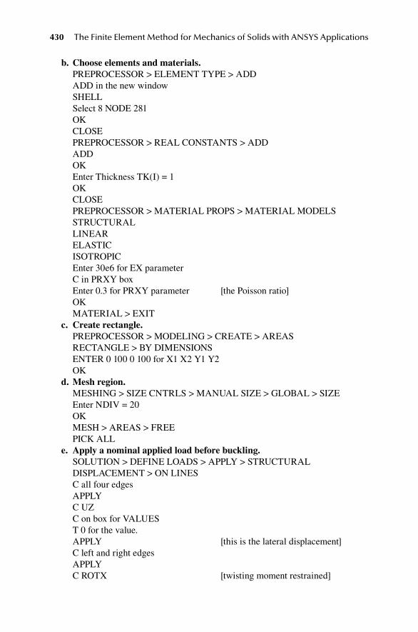
430 The Finite Element Method for Mechanics of Solids with ANSYS Applications
b. Choose elements and materials.PREPROCESSOR > ELEMENT TYPE > ADDADD in the new windowSHELLSelect 8 NODE 281 OKCLOSE PREPROCESSOR > REAL CONSTANTS > ADDADDOKEnter Thickness TK(I) = 1OKCLOSEPREPROCESSOR > MATERIAL PROPS > MATERIAL MODELSSTRUCTURALLINEARELASTICISOTROPICEnter 30e6 for EX parameter C in PRXY boxEnter 0.3 for PRXY parameter [the Poisson ratio]OKMATERIAL > EXIT
c. Create rectangle.PREPROCESSOR > MODELING > CREATE > AREASRECTANGLE > BY DIMENSIONSENTER 0 100 0 100 for X1 X2 Y1 Y2OK
d. Mesh region.MESHING > SIZE CNTRLS > MANUAL SIZE > GLOBAL > SIZEEnter NDIV = 20OKMESH > AREAS > FREEPICK ALL
e. Apply a nominal applied load before buckling.SOLUTION > DEFINE LOADS > APPLY > STRUCTURAL DISPLACEMENT > ON LINESC all four edgesAPPLYC UZ C on box for VALUEST 0 for the value.APPLY [this is the lateral displacement]C left and right edgesAPPLYC ROTX [twisting moment restrained]
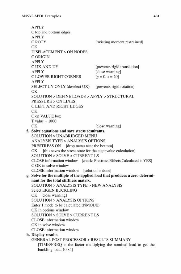
ANSYS APDL Examples 431
APPLYC top and bottom edgesAPPLYC ROTY [twisting moment restrained]OKDISPLACEMENT > ON NODESC ORIGINAPPLYC UX AND UY [prevents rigid translation]APPLY [close warning]C LOWER RIGHT CORNER [y = 0, x = 20]APPLYSELECT UY ONLY (deselect UX) [prevents rigid rotation]OK SOLUTION > DEFINE LOADS > APPLY > STRUCTURAL PRESSURE > ON LINESC LEFT AND RIGHT EDGESOKC on VALUE boxT value = 1000 OK [close warning]
f. Solve equations and save stress resultants.SOLUTION > UNABRIDGED MENUANALYSIS TYPE > ANALYSIS OPTIONS PRESTRESS ON [drop menu near the bottom] OK [this saves the stress state for the eigenvalue calculation]SOLUTION > SOLVE > CURRENT LSCLOSE information window [check: Prestress Effects Calculated is YES]C OK in solve windowCLOSE information window [solution is done]
g. Solve for the multiple of the applied load that produces a zero determi-nant for the total stiffness matrix.SOLUTION > ANALYSIS TYPE > NEW ANALYSISSelect EIGEN BUCKLINGOK [close warning]SOLUTION > ANALYSIS OPTIONSEnter 1 mode to be calculated (NMODE)OK in options windowSOLUTION > SOLVE > CURRENT LSCLOSE information windowOK in solve windowCLOSE information window
h. Display results.GENERAL POST PROCESSOR > RESULTS SUMMARY [TIME/FREQ is the factor multiplying the nominal load to get the
buckling load, 10.84]

432 The Finite Element Method for Mechanics of Solids with ANSYS Applications
CLOSEC GENERAL POST PROC > READ RESULTS > FIRST SETC GENERAL POST PROC > PLOT RESULTS > DEFORMED SHAPEC DEF & UNDEF C OK Rotate around the x-axis to see buckled mode shape using the Pan–Zoom–
Rotate tool or the icons on the right side.
15.30 heated rectangular rod
A square rod with initial temperature T = 0 is heated on both ends to a temperature T = 1. The nondimensional length is 1 and the nondimensional material properties are κ = 1, ρ = 1, and c = 1. The temperature rise at the middle is sought. The four-node thermal element Plane55 is used.
a. Activate ANSYS and set preferences.FILE > CHANGE JOBNAMEEnter job30 as job nameNew Log = YESOKPREFERENCESTHERMALOK
b. Choose element and material.PREPROCESSORELEMENT TYPE > ADDADDTHERMAL SOLID > QUAD 4NODE 55 [plane55 element]OKCLOSEMATERIAL PROPS > TEMPERATURE UNITSSelect CELSIUSOKMATERIAL PROPS > MATERIAL MODELSTHERMALCONDUCTIVITY > ISOTROPICEnter KXX = 1 [nondimensional parameters]OKSPECIFIC HEATEnter C = 1OKDENSITYEnter DENS = 1OKMATERIAL > EXIT

ANSYS APDL Examples 433
c. Create geometry.MODELING > CREATE > AREAS > RECTANGLE > BY
DIMENSIONSEnter X1 = 0, X2 = 1, Y1 = 0, Y2 = 0.1OK
d. Mesh region.MESHING > SIZE CNTRLS > MANUAL SIZE > GLOBAL > SIZEEnter SIZE = 0.05OKMESH > AREAS > FREEPICK ALL [2 × 20 grid of elements]
e. Apply boundary and initial conditions.LOADS > DEFINE LOADS > SETTINGS > UNIFORM TEMPEnter TUNIF = 0 [initial condition]OKAPPLY > THERMAL > TEMPERATURE > ON LINESPick the LINES at X = 0 and X = 1 [right and left ends]OKSelect TEMP and enter VALUE = 1OKHEAT FLUX > ON LINESSelect lines Y = 0, and Y = 0.1 [top and bottom]OKEnter VALI = 0OK
f. Solve for temperature history.SOLUTIONANALYSIS TYPE > NEW ANALYSISSelect TRANSIENTOKOK [to accept FULL]LOAD STEP OPTSOUTPUT CTRLS > DB/RESULTS FILESelect EVERY SUBSTEPOKTIME/FREQUENCY > TIME AND SUBSTPSEnter TIME = 0.5 NSUBST = 50 [small steps to approximate the
exponential]Select STEPPED [ANSYS actually ramps load up in
the first step]MAX STEPS = 50MIN STEPS = 50OKSOLVE > CURRENT LS

434 The Finite Element Method for Mechanics of Solids with ANSYS Applications
Close information windowOK in solve windowClose done window
g. Contour plot of temperature.GENERAL POSTPROCOR > READ RESULTS > BY TIME/FREQEnter TIME = 0.1OKPLOT RESULTS > CONTOUR PLOT > NODAL SOLU DOF SOLUTION > NODAL TEMPERATUREOK [note that the temperature varies only lengthwise]
h. View temperature history.PLOT ELEMENTSTIMEHIST POSTPROClose variable information windowDEFINE VARIABLESADDOK [for Nodal DOF result]PICK NODE AT X = 0.5 [the middle]OKEnter NAME = TOK [note that variable 2 is temp T at selected node]CLOSE windowLIST VARIABLESEnter NVAR1 = 2OK [temperature at each time is listed]Close windowGRAPH VARIABLESEnter NVAR1 = 2OK [graph of T vs. time appears]
15.31 heated cylIndrIcal rod
An unrestrained cylindrical rod with initial temperature T = 0 is heated on one end to a temperature T = 1. The nondimensional radius is 0.1, the nondimensional length is 1, and the nondimensional material properties are E = 1, ν = 0.3, α = 1, κ = 1, ρ = 1, and c = 1. Heat loss on the exterior is neglected. The temperature distribution and the deformations are axisymmetric. The four-node thermal element Plane 55 is used for the temperature calculation and the Plane 182 element is then automatically used for the thermal stress.
a. Activate ANSYS and set preferences.FILE > CHANGE JOBNAMEEnter job31 as the job nameSelect New Log = YESOKPREFERENCES

ANSYS APDL Examples 435
STRUCTURALTHERMALOK
b. Choose thermal element and thermal properties.PREPROCESSORELEMENT TYPE > ADDADDTHERMAL SOLID [QUAD 4NODE 55 selected]OKOPTIONSK3 = AXISYMMETRIC [X becomes radial (r), Y become longitudi-
nal (z)]OKCLOSEMATERIAL PROPS > TEMPERATURE UNITSSelect CELSIUSOKMATERIAL PROPS > MATERIAL MODELSTHERMAL CONDUCTIVITY > ISOTROPICEnter KXX = 1 [nondimensional parameters]OKSPECIFIC HEATEnter C = 1OKDENSITYEnter DENS = 1OKMATERIAL > EXIT
c. Create geometry.MODELING > CREATE > AREAS > RECTANGLE > BY DIMENSIONSEnter X1 = 0, X2 = 0.1, Y1 = 0, Y2 = 1OK
d. Mesh region.MESHING > SIZE CNTRLS > MANUAL SIZE > GLOBAL > SIZEEnter SIZE = 0.02OKMESH > AREAS > FREEPICK ALL [5 × 50 grid of elements]
e. Apply boundary and initial conditions.LOADS > DEFINE LOADS > SETTINGS > UNIFORM TEMPEnter TUNIF = 0 [initial condition]OKAPPLY > THERMAL > TEMPERATURE > ON LINESPick the LINE at Y = 0 [bottom end]OK
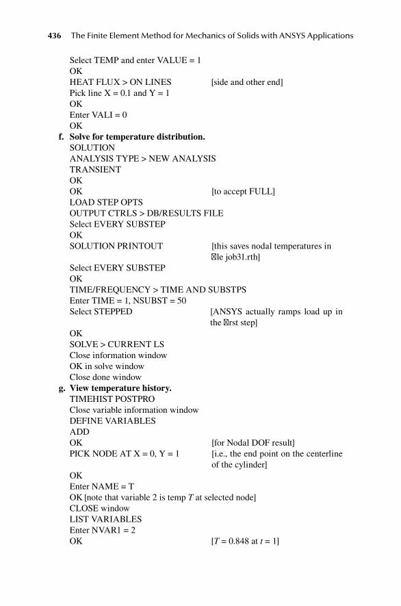
436 The Finite Element Method for Mechanics of Solids with ANSYS Applications
Select TEMP and enter VALUE = 1OKHEAT FLUX > ON LINES [side and other end]Pick line X = 0.1 and Y = 1OKEnter VALI = 0OK
f. Solve for temperature distribution.SOLUTIONANALYSIS TYPE > NEW ANALYSISTRANSIENTOKOK [to accept FULL]LOAD STEP OPTSOUTPUT CTRLS > DB/RESULTS FILESelect EVERY SUBSTEPOKSOLUTION PRINTOUT [this saves nodal temperatures in
file job31.rth]Select EVERY SUBSTEP OKTIME/FREQUENCY > TIME AND SUBSTPSEnter TIME = 1, NSUBST = 50 Select STEPPED [ANSYS actually ramps load up in
the first step]OKSOLVE > CURRENT LSClose information windowOK in solve windowClose done window
g. View temperature history.TIMEHIST POSTPROClose variable information windowDEFINE VARIABLESADDOK [for Nodal DOF result]PICK NODE AT X = 0, Y = 1 [i.e., the end point on the centerline
of the cylinder]OKEnter NAME = TOK [note that variable 2 is temp T at selected node]CLOSE windowLIST VARIABLESEnter NVAR1 = 2OK [T = 0.848 at t = 1]
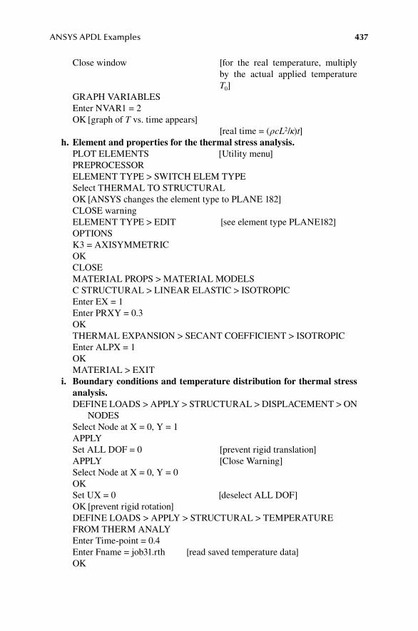
ANSYS APDL Examples 437
Close window [for the real temperature, multiply by the actual applied temperature T0]
GRAPH VARIABLESEnter NVAR1 = 2OK [graph of T vs. time appears]
[real time = (ρcL2/κ)t]h. Element and properties for the thermal stress analysis.
PLOT ELEMENTS [Utility menu]PREPROCESSORELEMENT TYPE > SWITCH ELEM TYPESelect THERMAL TO STRUCTURALOK [ANSYS changes the element type to PLANE 182]CLOSE warningELEMENT TYPE > EDIT [see element type PLANE182]OPTIONSK3 = AXISYMMETRICOKCLOSEMATERIAL PROPS > MATERIAL MODELSC STRUCTURAL > LINEAR ELASTIC > ISOTROPICEnter EX = 1Enter PRXY = 0.3OKTHERMAL EXPANSION > SECANT COEFFICIENT > ISOTROPICEnter ALPX = 1OKMATERIAL > EXIT
i. Boundary conditions and temperature distribution for thermal stress analysis.DEFINE LOADS > APPLY > STRUCTURAL > DISPLACEMENT > ON
NODESSelect Node at X = 0, Y = 1APPLYSet ALL DOF = 0 [prevent rigid translation]APPLY [Close Warning]Select Node at X = 0, Y = 0OK Set UX = 0 [deselect ALL DOF]OK [prevent rigid rotation]DEFINE LOADS > APPLY > STRUCTURAL > TEMPERATURE FROM THERM ANALYEnter Time-point = 0.4Enter Fname = job31.rth [read saved temperature data]OK

438 The Finite Element Method for Mechanics of Solids with ANSYS Applications
j. Solve for thermal stress.SOLUTIONANALYSIS TYPE > NEW ANALYSIS STATIC OKSOLVE > CURRENT LSClose Status windowOK solve windowClose solution done
k. View Results.GENERAL POSTPROCPLOT RESULTS > CONTOUR PLOT > NODAL SOLUTIONSTRESS > Y-COMPONENT [thermal stress]OKLIST RESULTS > NODAL SOLUTION > STRESS > Y-COMPONENTOK [for the real stress, multiply by EαT0]CLOSE
15.32 heated dISk
An unrestrained hollow cylinder rod with an internal radius of 5 in. and an outer radius of 10 in. is heated to a steady state. The temperature on the inner radius is 480°F and 75°F on the outer radius. Material properties: E = 2.9 × 10⁷ lb/in., ν = 0.3, ρ = 0.284 lbm/in.3, α = 6.67 × 10⁻⁶ 1/°F, κ = 8.092 10–4 BTU/s. in. °F, c = 0.1036 BTU/lbm. °F. Temperature distribution and thermal stress are to be determined. The four-node thermal element Plane 55 is used for the temperature calculation and the Plane 182 element is then automatically used to calculate the thermal stress. For a very long or very short cylinder, this problem is one-dimensional, but a ¼ cross section is maintained for clarity (Figure 15.25). The body is analyzed as a plane strain.
a. Activate ANSYS and set preferences.FILE > CHANGE JOBNAMEEnter job32 as job nameSelect NEW LOG = YESOKPREFERENCES
a
b
q = 0
q =
0 T2
T1
fIgure 15.25 Heated disk.

ANSYS APDL Examples 439
STRUCTURALTHERMALOK
b. Choose thermal element and thermal properties.PREPROCESSORELEMENT TYPE > ADDADDTHERMAL SOLID [QUAD 4NODE 55 selected]OKCLOSEMATERIAL PROPS > TEMPERATURE UNITSSelect FAHRENHEITOKMATERIAL PROPS > MATERIAL MODELSTHERMALCONDUCTIVITY > ISOTROPICEnter KXX = 8.092e – 4OKSPECIFIC HEATEnter C = 0.1036OKDENSITYEnter DENS = 0.284OKMATERIAL > EXIT
c. Create geometry.MODELING > CREATE > KEYPOINTS > IN ACTIVE CSEnter 1 at 5, 0APPLYEnter 2 at 10, 0APPLYEnter 3 at 0, 10APPLYEnter 4 at 0, 5OKWORKPLANE > CHANGE ACTIVE CS > TO GLOBAL
CYLINDRICALCREATE > LINES > LINES > IN ACTIVE CSPick KP 1 then 2Pick KP 1 then 4 [arc in cylindrical system]Pick KP 2 then 3 [arc in cylindrical system]Pick KP3 then 4OKCREATE > AREAS > ARBITRARY > BY LINESPick the lines sequentiallyOK

440 The Finite Element Method for Mechanics of Solids with ANSYS Applications
d. Mesh region.MESHING > SIZE CNTRLS > MANUAL > LINES > ALL
LINESEnter NDIV = 20OKMESH > AREAS > FREEPICK ALL [uniform 20 × 20 mesh]
e. Apply boundary conditions on temperature.LOADS > DEFINE LOADS > APPLY > THERMAL > TEMPERATURE >
ON LINESPick the inner arc APPLYSelect TEMP and enter VALUE = 480APPLYPick the outer arc OKEnter VALUE = 75OKAPPLY > THERMAL > HEAT FLUX > ON LINESPick the lines X = 0 and Y = 0OKVALUI = 0OK
f. Solve for temperature distribution and save results.SOLUTION [steady-state is the default]LOAD STEP OPTSOUTPUT CTRLSSOLU PRINTOUT [this saves nodal temperatures in file job32.
rth]Select LAST SUBSTEP OKSOLVE > CURRENT LS Close information windowOK in solve windowClose done window
g. View temperature distribution.GENERAL POSTPROC > PLOT RESULTSCONTOUR PLOT > NODAL SOLUDOF SOLUTION > NODAL TEMPERATUREOK [Contour plot shows axisymmetric
temperature]h. Change element for stress analysis.
PLOT ELEMENTS [Utility menu]PREPROCESSORELEMENT TYPE > SWITCH ELEM TYPESelect THERMAL TO STRUCTURAL

ANSYS APDL Examples 441
OK [ANSYS changes the element type to PLANE 182]
CLOSE warningELEMENT TYPE > EDIT > OPTIONSK3 = PLANE STRAINOKCLOSE
i. Mechanical properties.MATERIAL PROPS > MATERIAL MODELSC STRUCTURAL > LINEAR > ELASTIC > ISOTROPICEnter EX = 2.9e7Enter PRXY = 0.3OKTHERMAL EXPANSION > SECANT COEFFICIENT > ISOTROPICEnter ALPX = 6.67e−6MATERIAL > EXIT
j. Mechanical boundary conditions and thermal load.SOLUTION DEFINE LOADS > APPLY > STRUCTURAL > DISPLACEMENT > ON
LINESSelect Line Y = 0APPLYSet UY = 0 [symmetry]APPLY [Close Warning]Select Line X = 0OKSet UX = 0 [symmetry]OKDEFINE LOADS > APPLY > STRUCTURAL > TEMPERATURE FROM THERM ANALYEnter Time-point = 1Enter Fname = job32.rth [read saved temperature data]OK
k. Solve for thermal stress.SOLVE > CURRENT LSClose Status windowOK solve windowClose solution done
l. View results.GENERAL POSTPROCQUERY RESULTS > SUBGRID SOLUSTRESS > SXOKPick node at X = 0, Y = 5 τθθ = –70,678 lb/in.2
Pick node at X = 0, Y = 10 τθθ = 45,236 lb/in.2
OK

442 The Finite Element Method for Mechanics of Solids with ANSYS Applications
15.33 truSS contactIng a rIgId foundatIon
The truss is forced into contact with a rigid foundation (Figure 15.26) with L = 10, g = 0.3. Member 1 has A = 0.1 and E = 12,500. Member 2 has A = 0.2 and E = 12,500. There is no resistance to slip after contact. The loads are ramped up to Fx = 27 and Fy = 12.8. Equation 14.28 shows that the simultaneous loading causes contact at Fx = 13.94, Fy = 6.61, U = 0.6495. This is a node to surface contact. Use Contact Element 175, Target Element 169, and the Lagrange multiplier method with default parameters.
a. Activate ANSYS and select preferences.See example 15.3.
b. Set up parameters.PARAMETERS > SCALAR PARAMETERS >G = 0.3 [gap size]ACCEPTMU = 0 [friction factor]ACCEPTCLOSE
c. Element types, real constants, material properties.PREPROCESSORELEMENT TYPEADDADDLINK > 3D finit str 180 OKADDCONTACT > 2D TARGET 169OKADDPT-TO-SURF 175OKSelect TYPE 3 CONTA175
3L 3L
4L
gFx ,U Fy ,V
12
fIgure 15.26 Truss contact problem.

ANSYS APDL Examples 443
OPTIONSK2 = LAGRANGE METHODOKCLOSEREAL CONSTANTS > ADDADDCONTA175OKOK [accept defaults]ADDLINK1OKAREA = 0.1 [set 2]OKADDLINK1OKAREA = 0.2 [set 3]OKCLOSEMATERIAL PROPS > MATERIAL MODELSC STRUCTURAL > LINEAR > ELASTIC > ISOTROPICEX = 12500 [material 1]PRXY = 0.3 [not used]OKC FRICTION COEFFICIENTMU = 0OKMATERIAL > EXIT
d. Create nodes and elements.MODELING > CREATE NODES > IN ACTIVE CSNODE = 1X,Y,Z = 0,0,0APPLYNODE = 2X,Y,Z = 30,40,0APPLYNODE = 3X,Y,Z = −30,40,0OKELEMENTS > ELEM ATTRIBUTESTYPE = LINK1MAT = 1REAL = 2OK

444 The Finite Element Method for Mechanics of Solids with ANSYS Applications
AUTO/NUMBERED > THRU NODESPICK 1 AND 2OKELEMENTS > ELEM ATTRIBUTESTYPE = LINK1MAT = 1REAL = 3OKAUTO/NUMBERED > THRU NODESPICK 1 AND 3OKELEMENTS > ELEM ATTRIBUTESTYPE = CONTA175MAT = 1REAL = 1OKSURF / CONTACTNODE TO SURFOKPICK NODE 1OKMODELING > CREATE KEYPOINTS > IN ACTIVE CSNPT = 10X,Y,Z = +30,−g,0APPLYNPT = 11X,Y,Z = −30,−g,0OKLINES > LINES > IN ACTIVE CSPICK 10 THEN 11 IN THAT ORDER [so that the normal will have
the proper direction]OKMESHING > MESH ATTRIBUTES > DEFAULT ATTRIBSTYPE = TARGET169REAL = 1OKMESH > LINESPICK LINEOK [a target not overlaid is rigid]
e. Apply boundary conditions.LOADS > DEFINE LOADS > APPLY STRUCTURAL > DISPLACEMENT > ON NODESPICK NODES 2 AND 3OK

ANSYS APDL Examples 445
ALL DOFVALUE = 0OKFORCE/MOMENT > ON NODESPICK NODE 1OKAPPLYLAB = FXVALUE = −27 [i.e., to the left]APPLYPICK NODE 1OKLAB = FYVALUE = −12.8 [i.e., downward]OK
f. Solve for displacements.SOLUTIONUNABRIDGED MENULOAD STEP OPTSOUTPUT CONTROLS > DB RESULTS FILESELECT EVERY SUBSTEPOKTIME/FREQUENCY > TIME AND SUBSTEPSTIME = 1NSUBST = 50MINIMUM NO. = 50MAXIMUM NO. = 50OKSOLVE > CURRENT LSCLOSE INFO WINDOWOK IN SOLVE WINDOW [see graph of convergence]CLOSE SOLUTION IS DONE WINDOW
g. View results.GENERAL POSTPROCREAD RESULTSLAST SETPLOT RESULTS > DEFORMED SHAPEDEF + UNDEFORMED [displacement is magnified so thatOK the node appears to penetrate the
surface]LIST RESULTS > NODAL SOLUTIONCONTACT > STATUSOK [STAT = 2 indicates contact]CONTACT > PENETRATION [PENE = 0.0000, i.e., no
penetration]

446 The Finite Element Method for Mechanics of Solids with ANSYS Applications
CONTACT > PRESSURE [PRES = 12.000]CLOSELIST RESULTS > NODAL SOLUTIONDOF SOLUTION > X-COMPONENT OF DISPLACEMENTOK [UX = −1.1333]CLOSELIST RESULTS > NODAL SOLUTIONDOF SOLUTION > Y-COMPONENT OF DISPLACEMENTOK [UY = −0.3, i.e., gap closed]CLOSE
h. View time history.TIME HIST POSTPROC CLOSE INFO WINDOWDEFINE VARIABLES > ADD > NODAL DOF RESULTOKPICK NODE 1OKNAME = UXOK [variable 2 is UX]ADD > NODAL DOF RESULTOKPICK NODE 1OKNAME = UYSELECT UYOK [variable 3 is UY]CLOSELIST VARIABLESNVAR1 = 2NVAR2 = 3OK [note contact UY = −0.3, 0.629 ≤ UX ≤ −0.653 at
≤0.52 of total load]CLOSE
15.34 coMpreSSIon of a ruBBer cylInder BetWeen rIgId plateS
Coupling of nodes is introduced and subregions are used to control meshing.A long rubber cylinder is compressed between rigid plates (Figures 15.27 and
15.28). The cylinder is analyzed as a plane strain problem with R = 0.5 in., E = 500 lb/in.2 (rubber), ν = 0.499. Since the material is nearly incompressible, the mixed (U–P) formulation is used. Because of the double symmetry, only ¼ of the cylinder is modeled. The plane y = 0 is assumed to remain plane and the nodal displacements UY on the plane are coupled. A vertical displacement, d = 0.05 in. of the plane is imposed. The required force F and the contact region b are calculated. The expected results are given in Section 14.3.1.

ANSYS APDL Examples 447
a. Activate ANSYS and set analysis type to structural.See example 15.3.
b. Establish element type and material properties.PREPROCESSOR > ELEMENT TYPE > ADDC ADDC SOLID > 4 NODE 182 OKOPTIONSSET K3 TO PLANE STRAINSET K6 TO MIXED U/POKADDCONTACT > 2D TARGET 169 [surface-to-surface contact pair]OKADD2 ND SURF 171OKC TYPE 3 CONTA 171OPTIONS [accept defaults]OKCLOSE [Real Constants > add > add > CONTA171
could be used here to adjust contact parameters]PREPROCESSOR > MATERIAL PROP > MATERIAL MODELC STRUCTURAL > LINEAR > ELASTIC > ISOTOPIC
F
F
2Rxy
fIgure 15.27 Compressed cylinder.
KP 1
KP 2
UX
= 0
3
7
y
x 6
5
4
UY = – 0.05
fIgure 15.28 Subregions for one-quarter.
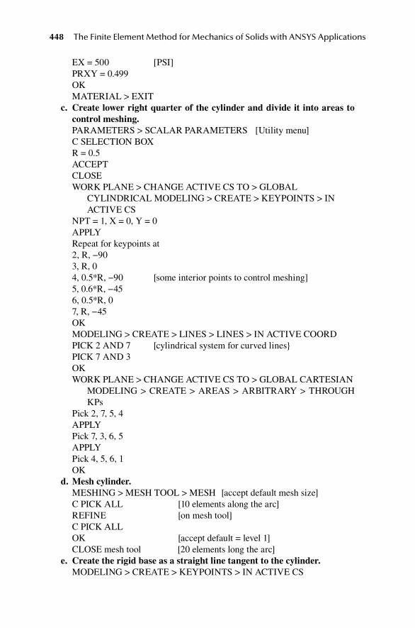
448 The Finite Element Method for Mechanics of Solids with ANSYS Applications
EX = 500 [PSI]PRXY = 0.499OKMATERIAL > EXIT
c. Create lower right quarter of the cylinder and divide it into areas to control meshing.PARAMETERS > SCALAR PARAMETERS [Utility menu]C SELECTION BOXR = 0.5ACCEPTCLOSEWORK PLANE > CHANGE ACTIVE CS TO > GLOBAL
CYLINDRICAL MODELING > CREATE > KEYPOINTS > IN ACTIVE CS
NPT = 1, X = 0, Y = 0APPLYRepeat for keypoints at2, R, −903, R, 04, 0.5*R, −90 [some interior points to control meshing]5, 0.6*R, −456, 0.5*R, 07, R, −45OKMODELING > CREATE > LINES > LINES > IN ACTIVE COORDPICK 2 AND 7 [cylindrical system for curved lines}PICK 7 AND 3OKWORK PLANE > CHANGE ACTIVE CS TO > GLOBAL CARTESIAN MODELING > CREATE > AREAS > ARBITRARY > THROUGH
KPsPick 2, 7, 5, 4APPLYPick 7, 3, 6, 5APPLYPick 4, 5, 6, 1OK
d. Mesh cylinder.MESHING > MESH TOOL > MESH [accept default mesh size]C PICK ALL [10 elements along the arc]REFINE [on mesh tool]C PICK ALLOK [accept default = level 1]CLOSE mesh tool [20 elements long the arc]
e. Create the rigid base as a straight line tangent to the cylinder.MODELING > CREATE > KEYPOINTS > IN ACTIVE CS

ANSYS APDL Examples 449
NPT = 10, X = +2 * R, Y = −RAPPLYNPT = 11, X = −2 * R, Y = −ROKMODELING > CREATE > LINES > LINES > IN ACTIVE COORDPick KP 10 then 11 [must pick in this order to get correct
normal]OK
f. Mesh rigid base.MESHING > MESH ATTRIBUTES > DEFAULT ATTRIBSTYPE = TARGE169OKPLOT > LINESMESH > LINES PICK the rigid base [defaults to one element]OK
g. Overlay contact elements on the surface of the cylinder.MODELING > CREATE > ELEMENTS > ELEM ATTRIBUTESTYPE = CONTA171OKSURF / CONTACT > SURF TO SURFOK [accept top surface]Pick about 10 nodes along the arc surface of the cylinder up from the
bottomOK [note outward normal to the elements on the
curved edge as required]h. Restrict the nodes on the plane of symmetry (Y = 0) to a common UY.
PREPROCESSOR > COUPLING > COUPLE DOFsPick nodes along the plane y = 0 by box [along the top]OKNSET = 1LAB = UY [makes the UY component the same]OK
i. Apply boundary conditions.LOADS > DEFINE LOADS > APPLY > STRUCTURAL > DISPLACEMENT > ON NODESPICK nodes along center line (x = 0) by boxOKUX = 0 [symmetry condition]OKDEFINE LOADS > APPLY > STRUCTURAL > DISPLACEMENT > ON
NODESPICK top right corner node (27) on symmetry line y = 0OK UY = −0.05 [note negative sign]OK

450 The Finite Element Method for Mechanics of Solids with ANSYS Applications
j. Solve problem step by step.SOLUTION > ANALYSIS TYPE > SOL’N CONTROLS Time at end of load step = 1Number of substeps = 10OKSOLUTION > SOLVE > CURRENT LSCLOSE information windowOK in solve window(Convergence information is displayed as solution is marched out.) CLOSE information window when solution is done
k. Display results.PLOT CTRLS > STYLE > DISPLACEMENT SCALING Select 1.0 [no magnification]OKPLOT CTRLS > NUMBERINGNode Numbers = ON [zoom in as required]GENERAL POST PROC > READ RESULTS > LAST SETGENERAL POST PROC > PLOT RESULTS > DEFORMED SHAPEOK and see deformed shape [apparent contact by nodes 1-3-4-5]GENERAL POST PROC > LIST RESULTS REACTION SOLUTION > FYOKRecord FY at node 27 [FY = −12.507]CLOSEGENERAL POST PROC > LIST RESULTS > NODAL SOLUTIONCONTACT > CONTACT STATUSOK [status = 2 for nodes 1-3-4-5 indicates
contact] [status = 1 for node 6 indicates near contact]CONTACT > CONTACT [p = 104.67 at node 1]
PRESSURECLOSE LIST > NODES [Utility menu]OKRecord X coordinates for nodes 5 and 6 [X5 = 0.12751, X6 =
0.16705]CLOSEGENERAL POST PROC > LIST RESULTS > NODAL SOLUTIONDOF SOLUTION > X COMPONENTOKRecord UX5 and UX6 [UX5 = 0.00291, UX6 = 0.00629] [deformed X-position of node 5 is X5 + UX5 =
0.13042] [deformed X-position of node 6 is X6 + UX6 =
0.17334]CLOSE [contact boundary at 0.13 < x < 0.17]

ANSYS APDL Examples 451
15.35 hertz contact proBleM
Use of local coordinate systems is introduced. A contact pair is created using the Contact Wizard of the ANSYS Contact Manager.
The contact between two long cylinders is analyzed by assuming double sym-metry (Figure 15.29). The following sample instructions are for R1 = 10 mm, R2 = 13 mm, ν1 = ν2 = 0.25, E1 = E2 = 30,000 N/mm2. The angle defining the potential contact region is α1 = α2 = 8°. Apply a displacement d = 0.1 and determine the total force, the maximum contact pressure, and the contact region. The theory is dis-cussed in Section 14.3.2.
a. Activate ANSYS and set preferences.See example 15.3.
b. Element types, real constants, material properties.PREPROCESSORELEMENT TYPEADDADDSOLID4 NODE 182 [PLANE 182 element]OKOPTIONSSet K3 to PLANE STRAINOKCLOSEMATERIAL PROPS > MATERIAL MODELSC STRUCTURAL > LINEAR > ELASTIC > ISOTROPIC
Contact surface
Target surface
xuy = 0
ux = 0
uy = d
α2
α1
y
E2ν2R2
E1ν1
Rt
fIgure 15.29 Contact between cylinders.

452 The Finite Element Method for Mechanics of Solids with ANSYS Applications
EX = 30000PRXY = 0.25OKMATERIAL > EXIT
c. Create the target (large cylinder) and mesh it. WORKPLANE [Utility menu]CHANGE ACTIVE CS TO > GLOBAL CYLINDRICALMODELING > CREATE KEYPOINTS > IN ACTIVE CS [for large cylinder]NPT = 1X,Y,Z = 0,0,0APPLYNPT = 2X,Y,Z = 13,0,0APPLYNPT = 3X,Y,Z = 13,82,0APPLYNPT = 4X,Y,Z = 13,90,0APPLYNPT = 5X,Y,Z = 11,90,0OKLINES > LINES > IN ACTIVE CSPICK 1 AND 5PICK 1 AND 2PICK 2 AND 3 [circular arc]PICK 3 AND 4PICK 4 AND 5OKWORKPLANE > LOCAL COORDINATE SYSTEMSCREATE LOCAL CS > AT SPECIFIED LOCPICK KP 4 (X,Y,Z) = 0,13,0OKKCS = CYLINDRICALOK [local cylindrical coordinate system
11 at KP 4]LINES > IN ACTIVE CSPICK 3 AND 5 [csys 11 necessary to get concave arc]OKWORKPLANE [Utility menu]CHANGE ACTIVE CS TO > GLOBAL CYLINDRICALAREAS > ARBITRARY > THROUGH KPsPICK 1,2,3,5APPLY

ANSYS APDL Examples 453
PICK 5, 3, 4OKMESHING > MESH TOOLSIZE CONTROLS GLOBL SETNDIV = 10OKMESH [in Mesh tool]PICK ALLCLOSE [mesh tool]PLOT CTRLS > NUMBERING > NODE NUMBERS ONOK
d. Create small cylinder and mesh it.WORKPLANE > CHANGE ACTIVE CS TO > GLOBAL CARTESIANWORKPLANE > LOCAL COORDINATE SYSTEMSCREATE LOCAL CS > AT SPECIFIED LOCEnter coordinates 0, 23, 0 [center of small cyl]OKKCN = 12 [new active CS]THXY = −90 [rotate X-axis downward]OK MODELING > CREATE KEYPOINTS > IN ACTIVE CS [for small cylinder]NPT = 11X,Y,Z = 0,0,0APPLYNPT = 12X,Y,Z = 10,0,0APPLYNPT = 13X,Y,Z = 10,8,0APPLYNPT = 14X,Y,Z = 10,90,0APPLYNPT = 15X,Y,Z = 8,0,0OKLINES > LINES > IN ACTIVE CSEnter 12,13 [on picking menu]APPLYEnter 13,14 [circular arc]APPLYEnter 14,11APPLYEnter 11,15APPLY

454 The Finite Element Method for Mechanics of Solids with ANSYS Applications
Enter 15,12OKWORKPLANE > CHANGE ACTIVE CS TO > SPECIFIED COORD SYSKCN = 11OKLINES > IN ACTIVE CSEnter 13,15 [csys 11 necessary to get
arc concave]OKWORKPLANE > CHANGE ACTIVE CS TO > SPECIFIED COORD SYSKCN = 12 [back to local coords for
small cyl]OKAREAS > ARBITRARY > THROUGH KPsEnter 12,13,15APPLYEnter 15,13,14,11OKMESHING > MESH TOOLSIZE CONTROLS GLOBL SETNDIV = 10OKMESH PICK AREAS 3 AND 4 [small cylinder]OK [zoom in and note nodes on
target surface: 202 to 212]CLOSE [mesh tool]
e. Create contact surfaces.PLOT CTRLS > NUMBERINGLINE NUMBERS ONPLOT > LINESZOOM IN ON CONTACT REGIONMODELING > CREATE > CONTACT PAIR [contact manager]WIZARD (LEFT MOST ICON) [lines and flexibility
selected]PICK TARGETSELECT CONTACT LINE ON [L4]
LOWER CYLINDEROKNEXT [lines and surface-to-
surface selected]PICK CONTACTSELECT CONTACT LINE ON UPPER [L7]
CYLINDEROKNEXT

ANSYS APDL Examples 455
CREATE [note: normals outward from each cylinder]
FINISH [note description of con-tact pair]
CLOSE CONTACT MANAGER [C on X] f. Apply supports.
WORKPLANE > CHANGE ACTIVE CS TO > GLOBAL CARTESIANZOOM TO FIT [logo on right]COUPLING/CEQN > COUPLE DOFsPICK NODES ON TOP EDGE BY BOX [of small cylinder]OKNSET = 1LAB = UYOKPLOT LINESLOADS > DEFINE LOADS > APPLY > STRUCTURAL DISPLACEMENT > ON LINESPICK BOTTOM LINE (Y = 0)APPLYUY VALUE = 0APPLYPICK FOUR VERTICAL LINES (X = 0)OKUXVALUE = 0OK
g. Apply displacement on upper plane.PLOT > ELEMENTSLOADS > DEFINE LOADS > APPLY > STRUCTURAL > DISPLACEMENT > ON NODESPICK UPPER RIGHT CORNER [node 293]OKUYVALUE = −0.1 [note the minus sign]OKSOLUTIONUNABRIDGED MENULOAD STEP OPTSTIME/FREQUENCY > TIME AND SUBSTEPSTIME = 1NSUBST = 10OK
h. Solve for displacement and stress.SOLUTION > SOLVE > CURRENT LSCLOSE INFO WINDOW

456 The Finite Element Method for Mechanics of Solids with ANSYS Applications
OK CLOSE solution is done
i. View results.PLOT CTRLS > STYLE > DISPLACEMENT SCALINGSelect 1.0OKGENERAL POSTPROCPLOT RESULTS > DEFORMED SHAPEOKPLOT CTRLS > NODE NUMERS ONZoom in to see contact nodes: last one is 206 or 207LIST RESULTS > REACTION SOLUTIONOK [FY = −314 at node 293]CLOSELIST RESULTS > NODAL SOLUTION CONTACT > STATUS [STAT = 2 indicates contact at
node 206]OK [STAT = 1.5 indicates near con-
tact at node 207]Note pressure at center node [731 at node 202]Note furthest node in contact [node 206]Note location of next node [node 207]LIST NODES OKNote x-coordinate of last contact node [0.41876 at node 206]Note x-coordinate of next node [0.55822 at node 207]CLOSELIST RESULTS > NODAL SOLUTIONDOF SOLUTION > X COMPONENTOKRecord UX5 and UX6 [UX206 = −0.00534, UX207 =
−0.00589] [deformed X-position of node
206 is X + UX = 0.41342] [deformed X-position of node
207 is X + UX = 0.55233]CLOSE [contact boundary at 0.413 < x <
0.552]
15.36 elaStIc rod IMpactIng a rIgId Wall
This example demonstrates the use of the Solution Controls menu for transient analy-sis. The analysis uses node to surface contact, contact element 175, target element 169, using the default Augmented Lagrangian method with increased contact stiff-ness FKN. The rod (Figure 15.30) is made of steel: A = 1 in.2, E = 2.92 × 10⁷ lb/in.2,

ANSYS APDL Examples 457
ρ = 0.73 × 10⁻³ lbf-s2/in.4 The rod (Link element) approaches the wall with initial velocity V = 200 in./s2 from a gap of 0.01 in.
a. Activate ANSYS and set preferences.See example 15.3.
b. Element types, real constants, material properties.PREPROCESSORELEMENT TYPEADDADDLINK > 2D SPAR 1 OKADDCONTACT > 2D TARGET 169OKADDPT-TO-SURF 175OKSelect TYPE 3 CONTA175OPTIONSOK [accept augmented Lagrangian method]CLOSEREAL CONSTANTS > ADDADDLINK180OKAREA = 1 [set 1]OKADDCONTA175OK [set 2]FKN = 10 [increase contact stiffness to reduce penetration]OKCLOSEMATERIAL PROPS > MATERIAL MODELSC STRUCTURAL > LINEAR > ELASTIC > ISOTROPICEX = 2.92E7
Rigidwall
0.0110
V
A, E, ρ
fIgure 15.30 Rod impacts wall.

458 The Finite Element Method for Mechanics of Solids with ANSYS Applications
PRXY = 0.3 [not used]OKC DENSITYDENS = 0.73e−3OKMATERIAL > EXITPARAMETERS > SCALAR PARAMETERS G = 0.01 [gap size]ACCEPTCLOSE
c. Create line and mesh it.MODELING > CREATE KEYPOINTS > IN ACTIVE CSNPT = 1X,Y,Z = −10−G,0,0 [end of the rod]APPLYNPT = 2X,Y,Z = −G,0,0 [end of the rod]OKMODELING > CREATE > LINES > LINES > IN ACTIVE CSPick KP1 AND KP2OKMESHING > SIZE CNTRLS > MANUAL SIZE > GLOBAL >
SIZENDIV = 20 OKMESH > LINESPICK ALLPLOT CTRLS > WINDOW CONTROLS > WINDOW OPTIONS/TRIAD = AT BOTTOM LEFTOK [moves axis symbols out of the way]
d. Add contact elements.MODELING > CREATE > ELEMENTSELEM ATTRIBUTESTYPE = CONTA175REAL = 2OKSURF / CONTACTNODE TO SURFOKPICK NODE ON RIGHT END (2)OKMODELING > CREATE > KEYPOINTS > IN ACTIVE CSNPT = 10X,Y,Z = 0,2,0

ANSYS APDL Examples 459
APPLYNPT = 11X,Y,Z = 0,−2,0OKLINES > LINES > IN ACTIVE CSPICK 10 THEN 11 IN THAT ORDER [to get the correct normal]OKMESHING > MESH ATTRIBUTES > DEFAULT ATTRIBSTYPE = TARGET169OK REAL = 2 selected]MESH > LINESPICK LINE FROM KP10 TO KP11OK
e. Apply boundary and initial conditions.LOADS > DEFINE LOADS > APPLY
STRUCTURAL > DISPLACEMENT > ON NODESPICK NODES ON THE ROD BY A BOXOKUYVALUE = 0OKAPPLY > INITIAL CONDIT’N > DEFINEPICK NODES ON ROD BY BOXOKLab = UXVALUE2 = 200 [initial velocity]OK
f. Solve for displacements.SOLUTIONANALYSIS TYPE > NEW ANALYSIS > TRANSIENTOKLUMPM = YESOKSOL’N CONTROLS [Small Displacement Transient
selected]Time at end of loadstep = 2e−4Number of substeps = 100Max no. of substeps = 100Min no. of substeps = 100Write Items to Results File = All Solution ItemsFrequency = Write Every SubstepOKSOLVE > CURRENT LSCLOSE INFO WINDOW

460 The Finite Element Method for Mechanics of Solids with ANSYS Applications
OK IN SOLVE WINDOWCLOSE SOLUTION IS DONE WINDOW
g. View history of displacement.TIME HIST POSTPROC CLOSE INFO WINDOWDEFINE VARIABLES > ADD > NODAL DOF RESULTOKPICK RIGHT END NODE 2OKNAME = UOK [variable 2 is UX at node 2]CLOSEGRAPH VARIABLESNVAR1 = 2OK [print if desired]
15.37 curve fIt for nonlInear elaStIcIty uSIng Blatz–ko Model
The ANSYS curve fit for hyperelastic materials is used to interpret test data.The problem is an analysis of a tensile test (unit cube) using “test data” and the
ANSYS Curve Fit to determine the constant in the Blatz–Ko material model. One eight-node brick is used with unit side lengths since one element is an exact model of the tensile test (Figure 15.31).
The experimental data for a tensile test must be entered manually or placed in a text file. The first column must be the extension (α1 – 1) and the second column, separated by a space or comma, must be the nominal stress (P11). In the following example, the file BK.txt has a content that was calculated using the Blata–Ko model with μ = 100 as follows:
0 00.1 20.220.2 33.420.3 42.19
103
10
1010
465
UX = UY = UZ = 0 x2z
y
7UX = UZ = 0 1
UX = UY = 0
8UX = 0
fIgure 15.31 3D tensile test: fixed load.

ANSYS APDL Examples 461
The axial load is ramped up to P11 = 40. Minimum supports are imposed to prevent rigid displacement.
a. Activate ANSYS and set analysis type to structural.See example 15.3.
b. Establish element type, material properties, and mesh the object.PREPROCESSOR > ELEMENT TYPE > ADDADDHYPERELASTIC3D 8 NODE 185 [this is SOLID185 element]OKCLOSEPREPROCESSOR > MATERIAL PROP > MATERIAL MODELSTRUCTURALNONLINEARELASTICHYPERELASTICCURVE FITTING [define material behavior window]READ FROM FILE [directory listing]C BK.txt [file containing tensile test data]OPEN [data are read in]NEXTCURVE FITSHYPERELASTICBLATZ–KO (FOAM)SOLVE [returns μ = 100.01]OK [curve fit done]PLOT [stress–strain curve]SAVE AND CLOSE [material constant for the model]MATERIAL > EXITPREPROCESSOR > MODELING > CREATE > VOLUMESBLOCK > BY DIMENSIONST 0 1, 0 1, 0 1 for X1, X2, Y1, Y2, Z1, Z2C OK and the region appears showing the x–y planePLOT CTRLS > NUMBERINGC box after Node numbers to turn them ONOKPREPROCESSOR > MESHING > MESH TOOLC SIZE CONTROLS: GLOBAL > SETC box for NDIVT 1 in NDIV box [one element is exact for the uniform
extension]OKC SHAPE: HEX [this forces a brick instead of the default
tetrahedron]MESH

462 The Finite Element Method for Mechanics of Solids with ANSYS Applications
PICK ALL (node numbers appear)CLOSE (Mesh Tool)
c. Apply boundary conditions. First, rotate the element so that you can see the base (x = 0) with nodes 1-2-
5-8. This can be done in the dynamic model mode, which is inter active: on the right-hand side is a menu with 3D pictures of a block. Click on the but-ton at the end of the list that shows two elements (Dynamic Model Mode). The cursor changes to a rotation symbol. Hold down the right mouse button to rotate the element interactively until you can see the face 1-2-5-8.LOADS > DEFINE LOADS > APPLY > STRUCTURAL DISPLACEMENT > ON NODESC on node 2 (at the origin)APPLYALL DOFC on box for VALUEST 0 for the value of the displacement componentsAPPLYREPEAT THIS PROCESS TO SET UX AND UZ TO ZERO AT NODE 1REPEAT THIS PROCESS TO SET UX AND UY TO ZERO AT NODE 5REPEAT THIS PROCESS TO SET UX TO ZERO AT NODE 8[This prevents rigid body motion and keeps the base in the Y−Z plane, but
allows contraction.]ROTATE THE ELEMENT so that you can see the face x = 1 with nodes
3-4-6-7DEFINE LOADS > APPLY > STRUCTURAL > FORCE > ON NODESC ON EACH NODE 3-4-6-7 OKT 10 for the value of FX [P11 = 40]OK
d. Solve for displacements and stresses. The total load is specified, then reached by ramping up in small time steps.
Results are saved after each time step.SOLUTION > UNABRIDGED MENUANALYSIS TYPE > ANALYSIS OPTIONS Set NLGEOM ON [this is for K0]Set Stress Stiff ON (SSTIF at the bottom) [this is for K1]OKSOLUTION > LOAD STEP OPTS > OUTPUT CTRLS > DB/RESULTS
FILEFile write frequency: select “every substep”OKSOLUTION > LOAD STEP OPTS > TIME/FREQUENC > TIME/TIME
STEPTime at end of load step: enter 1Time step size: enter 0.1Select RAMPED

ANSYS APDL Examples 463
Automatic time stepping: ONMinimum time step size: enter 0.05Maximum time step size: enter 0.1OKSOLUTION > SOLV CURRENT LSCLOSE information windowC OK in solve window(Convergence information is displayed as solution is marched out.)CLOSE information window when solution is done
e. Display results: List displacements of selected nodes after each time step.GENERAL POST PROC > PLOT RESULTS > DEFORMED SHAPEDEF & UNDEF OK and see deformed shapeGENERAL POST PROC > LIST RESULTSNODAL SOLUTIONDOF SOLUTION > X-Component of displacementOK [you should have UX = 0.271 at
node 4]CLOSEELEMENT SOLUTIONSTRESS > X-COMPONENT OF STRESSOK [you should have SX = 45.1; this is
the true stress T11]CLOSETIME HIST POSTPROCClose windowDEFINE VARIABLESADDSelect Nodal DOF ResultOKT 4 in the box for “list of items” [this is another way of picking the
node]OKEnter name: UXSelect Translation UXOK TIME HIST POSTPROC > DEFINE VARIABLESADDELEMENT RESULTSOKT 1 for the list of items (this is the element number)OKT 4 for the list of items (this is the node number for stress
output)OKEnter name SX
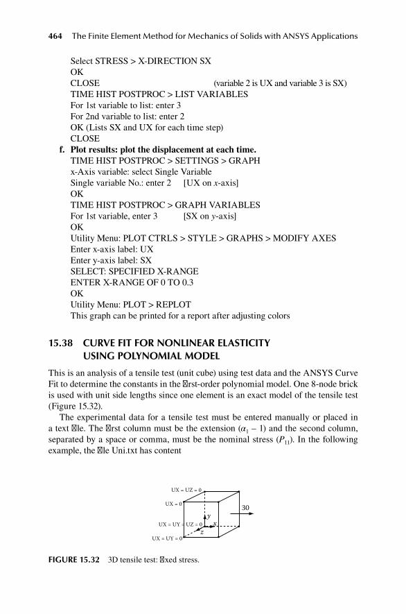
464 The Finite Element Method for Mechanics of Solids with ANSYS Applications
Select STRESS > X-DIRECTION SXOK CLOSE (variable 2 is UX and variable 3 is SX)TIME HIST POSTPROC > LIST VARIABLESFor 1st variable to list: enter 3For 2nd variable to list: enter 2OK (Lists SX and UX for each time step)CLOSE
f. Plot results: plot the displacement at each time.TIME HIST POSTPROC > SETTINGS > GRAPHx-Axis variable: select Single VariableSingle variable No.: enter 2 [UX on x-axis]OKTIME HIST POSTPROC > GRAPH VARIABLESFor 1st variable, enter 3 [SX on y-axis]OKUtility Menu: PLOT CTRLS > STYLE > GRAPHS > MODIFY AXESEnter x-axis label: UXEnter y-axis label: SXSELECT: SPECIFIED X-RANGEENTER X-RANGE OF 0 TO 0.3OKUtility Menu: PLOT > REPLOTThis graph can be printed for a report after adjusting colors
15.38 curve fIt for nonlInear elaStIcIty uSIng polynoMIal Model
This is an analysis of a tensile test (unit cube) using test data and the ANSYS Curve Fit to determine the constants in the first-order polynomial model. One 8-node brick is used with unit side lengths since one element is an exact model of the tensile test (Figure 15.32).
The experimental data for a tensile test must be entered manually or placed in a text file. The first column must be the extension (α1 – 1) and the second column, separated by a space or comma, must be the nominal stress (P11). In the following example, the file Uni.txt has content
30
UX = UY = UZ = 0 xz
y
UX = UZ = 0
UX = UY = 0
UX = 0
fIgure 15.32 3D tensile test: fixed stress.

ANSYS APDL Examples 465
0 00.0341 9.710.0697 18.860.1068 27.460.1453 35.550.1850 43.13
These data are taken from Table 13.1.Experimental data for volumetric strain must list the volume ratio (J) in the first
column and the mean pressure (p) in the second column. If no volumetric strain data are entered, the model is assumed to be incompressible. The file Vol.txt has the content
0.98 100.96 200.94 30
which is the exact values for κ = 500 or d = 0.004.The axial stress is ramped up to T11 = 30. Minimum supports are imposed to pre-
vent rigid displacement.
a. Activate ANSYS and set analysis type to structural.See example 15.3.
b. Establish element type.PREPROCESSOR > ELEMENT TYPE > ADDADDHYPERELASTICC 3D 8 NODE 185 [this is SOLID185 element]OKCLOSE
c. Material properties by a curve fit.PREPROCESSOR > MATERIAL PROP > MATERIAL MODELSTRUCTURALNONLINEARELASTICHYPERELASTICCURVE FITTING [define material behavior window]READ FROM FILE [directory listing]C Uni.txt [file containing tensile test data]OPEN [data are read in]NEXT [table for biaxial data appears]NEXTOK [no biaxial data warning]NEXT [table for shear data appears]OK [no shear data]NEXT [table for simple shear data appears]

466 The Finite Element Method for Mechanics of Solids with ANSYS Applications
OK [no data for simple shear]NEXT [table for volumetric test data appears]READ FROM FILEC Vol.TXT [file containing volumetric data]OPENNEXTHYPERELASTICPOLYNOMIALC 1st ORDERSOLVE [returns C10 = 21.9, C01 = 28.1, d = 0.004]OK [curve fit done]PLOT [stress–strain curves]SAVE AND CLOSE [material constants for the model]MATERIAL > EXIT
d. Create geometry.PREPROCESSOR > MODELING > CREATE > VOLUMES > BLOCK >
BY DIMENSIONST 0 1, 0 1, 0 1 for X1,X2,Y1,Y2, Z1,Z2C OK and the region appears showing the x–y planePLOT CTRLS > NUMBERINGC box after Node numbers to turn them ONOK
e. Mesh as one element.PREPROCESSOR > MESHING > MESH TOOLSIZE CONTROLS > GLOBAL > SETC box for NDIVT 1 in NDIV box [one element is exact for the uniform extension]OKSHAPE: HEX [this forces a brick instead of the default tetrahedron]MESHPICK ALL (node numbers appear)CLOSE (Mesh Tool)
f. Apply boundary conditions. First, rotate the element so that you can see the base (x = 0) with nodes
1-2-5-8. This can be done in the dynamic model mode, which is interac-tive: on the right-hand side is a menu with 3D pictures of a block. Click on the button at the end of the list that shows two elements (Dynamic Model Mode). The cursor changes to a rotation symbol. Hold down the right mouse button to rotate the element interactively until you can see the face 1-2-5-8.LOADS > DEFINE LOADS > APPLY > STRUCTURALDISPLACEMENT > ON NODESC on node 2 (at the origin)APPLYC ALL DOFC on box for VALUES

ANSYS APDL Examples 467
T 0 for the value of the displacement componentsC APPLYREPEAT THIS PROCESS TO SET UX AND UZ TO ZERO AT NODE 1REPEAT THIS PROCESS TO SET UX AND UY TO ZERO AT NODE 5REPEAT THIS PROCESS TO SET UX TO ZERO AT NODE 8[This prevents rigid body motion and keeps the base in the Y–Z plane, but
allows contraction.]ROTATE THE ELEMENT so that you can see the face x = 1 with nodes
3-4-6-7DEFINE LOADS > APPLY > STRUCTURAL > PRESSURE > ON
AREASC ON THE FACE 3-4-6-7 OKT −30 for the value [T11 = 30, negative pressure]C OK [close warning window]
g. Solve for displacements and stresses. The total load is specified, then reached by ramping up in small time steps.
Results are saved after each time step.SOLUTION > UNABRIDGED MENUANALYSIS TYPE > ANALYSIS OPTIONSSet NLGEOM ON [this is for K0]Set Stress Stiff ON (SSTIF at the bottom) [this is for K1]OKSOLUTION > LOAD STEP OPTS > OUTPUT CTRLS > DB/RESULTS
FILEFile write frequency: select “every substep”OKSOLUTION > LOAD STEP OPTS > TIME/FREQUENC > TIME/TIME
STEPTime at end of load step: enter 1Time step size: enter 0.1Select RAMPEDAutomatic time stepping: ONMinimum time step size: enter 0.05Maximum time step size: enter 0.1OKSOLUTION > SOLV CURRENT LSCLOSE information windowC OK in solve window(Convergence information is displayed as solution is marched out.)CLOSE information window when solution is done
h. Display results: List displacements of selected nodes after each time step.GENERAL POST PROC > PLOT RESULTS > DEFORMED SHAPEDEF & UNDEF OK and see deformed shapeGENERAL POST PROC > LIST RESULTS

468 The Finite Element Method for Mechanics of Solids with ANSYS Applications
NODAL SOLUTIONDOF SOLUTION > X-Component of displacementOK [you should have UX =
0.1149 at node 4]CLOSEELEMENT SOLUTIONSTRESS > X-COMPONENT OF STRESSOK [you should have SX = 30.00;
this is the true stress T11]CLOSETIME HIST POSTPROC Close windowDEFINE VARIABLESADDSelect Nodal DOF ResultOKT 4 in the box for “list [this is another way of picking the node]
of items”OKEnter name: UXSelect Translation UXOK TIME HIST POSTPROC > DEFINE VARIABLESADDELEMENT RESULTSOKT 1 for the list of items (this is the element number)OKT 4 for the list of items (this is the node number for stress output)OKEnter name SXSelect STRESS > X-DIRECTION SXOK CLOSE (variable 2 is UX and variable 3 is SX) TIME HIST POSTPROC > LIST VARIABLESFor 1st variable to list: enter 3For 2nd variable to list: enter 2OK (Lists SX and UX for each time step)CLOSE
i. Plot results: plot the displacement at each time.TIME HIST POSTPROC > SETTINGS > GRAPHx-Axis variable: select Single VariableSingle variable no.: enter 2 [UX on x-axis]OKTIME HIST POSTPROC > GRAPH VARIABLES

ANSYS APDL Examples 469
For 1st variable, enter 3 [SX on y-axis]OKUtility Menu: PLOT CTRLS > STYLE > GRAPHS > MODIFY AXESEnter x-axis label: UXEnter y-axis label: SXSELECT: SPECIFIED Y-RANGEENTER Y-RANGE OF 0 TO 50SELECT: SPECIFIED X-RANGEENTER X-RANGE OF 0 TO 0.2OKUtility Menu: PLOT > REPLOTThis graph can be printed for a report after adjusting colors
BIBlIography
Alawadhi, E. M., Finite Element Simulations Using ANSYS, CRC Press, Boca Raton, FL, 2010.
Madenci, E., and I. Guven, The Finite Element Method and Applications in Engineering Using ANSYS, Springer, New York, 2006.
Moaveni, S., Finite Element Analysis, Theory and Applications with ANSYS, 3rd ed., Prentice Hall, Upper Saddle River, NJ, 2008.
Stolarski, T. A., Y. Nakasone, and S. Yoshimoto, Engineering Analysis with ANSYS Software, Elsevier, New York, 2006.

471
16 ANSYS Workbench
This book is mainly about understanding the foundations of finite element analysis. But the ultimate goal is, of course, to apply the finite element method (FEM) to real material bodies. This means application to complex geometries. Workbench provides the means.
Workbench is a fully developed Computer Aided Engineering package. The exam-ples in Chapter 15 use the original ANSYS program that has been renamed ANSYS APDL. The tools for constructing the geometry of the material body using APDL are somewhat rudimentary. For complicated figures, you can use a CAD program to draw the figure and then import the geometry to ANSYS. Workbench eliminates that step. It has all of the tools of a CAD program and will automatically interface with the finite element analysis.
Workbench is especially useful for analyses that involve interaction of solid mechanics, heat transfer, fluid mechanics, and electrodynamics of materials, so called multiphysics problems. However, we will only consider here solid mechanics and heat conduction.
Product demonstrations, animated tutorials, and training materials are provided by ANSYS for existing customers through the Customer Portal: http://www1.ansys .com/customer/. This is a good place to start, but the instructions are not very detailed. New users should utilize one of the sources listed in the appended bibliography.
16.1 tWo- and three-dIMenSIonal geoMetry
The basic mouse operations are as follows. The left mouse button is used to click a single selection; click and hold to sweep for a continuous selection, or combine with the control key for multiple selection. The middle button is used for a rotation by click and hold, or a scroll wheel can be used to zoom in or out. The right mouse but-ton is clicked to obtain a context menu, or used to click and drag for a box zoom.
The program is initiated by
Start > All Programs > Ansys 12.1 > Workbench
After awhile the Workbench window appears with menu bars along the top, a graphics window (project schematic window) on the right, and a toolbox menu on the left.
Click on the + Sign to Expand the Component System Menu Double Click Component Systems > Geometry
This introduces into the project schematic window a schedule of tasks. In this case, the only task is to create a geometric figure.
Double Click on the Geometry task (not the Geometry heading)
472 The Finite Element Method for Mechanics of Solids with ANSYS Applications
This starts the software package called the Design Modeler within which the 2D or 3D body can be constructed. A menu appears in which one must select the units to be used for the drawing. Select the units and click OK. Then click Sketching in the lower left menu box to get the Sketching toolbox menu with submenus for Draw, Modify, Dimensions, Constraints, and Settings. Each menu has icons and names that are more or less self-explanatory. Their use will be demonstrated in the following examples. The most commonly used Draw Tools are the Line Tool for straight lines, and the Polyline Tool for open or closed polygonal figures. Click on a point for each apex, but do not drag out the line by holding down the mouse button. A rough figure is sketched with the Draw Tools without concern for the dimensions.
The Constraints Toolbox contains tools for restricting Symmetry of figures, iden-tifying Parallel Lines, lines of Equal Length, and so forth. Certain constraints are automatic: An H will appear if the line is horizontal; a V will appear if a line is verti-cal; a C will appear if the selected point falls on an existing line; a P will appear if a selected point is coincident with an existing point; etc.
The Dimensions Toolbox is used to impose the desired dimensions on the figure. The figure is drawn approximately. Next, one typically picks a line or a point for the origin of a dimension and then another point for the end of the dimension, then a point for the location of the dimension line. The value of the dimension is entered in the Detail Box, and the size of the figure is automatically adjusted. The Modify Toolbox can be used to insert fillets at corners, trim away extra construction lines, extend the drawing by Replicate of parts, and so forth.
A three-dimensional drawing is typically constructed by Extrude, Revolve, or Sweep of a 2D sketch. For plane stress, plane strain, plate, or shell analysis, it is nec-essary to first associate a surface with the 2D sketch of the body.
16.2 StreSS analySIS
In the startup toolbox, the Analysis Systems menu contains a list of tasks that can be executed using Workbench. If one double clicks on Static Structural (ANSYS), for example, a menu of subtasks to be performed appears in the Project Schematic (Graphics) window:
Static Structural (ANSYS) Engineering Data Geometry Model Setup Solution Results
The Engineering Data task includes the selection of a material.If a geometric figure has been previously constructed, this task is opened first and
then associated with the stress analysis by dragging the geometry to the Geometry task. A double click on Model starts the Mechanical task in which the finite element analysis is formulated. The desired output is set up in the Solution task.

ANSYS Workbench 473
The choice of element type and the mesh layout can be automatically generated by using default parameters of Workbench. The element type used and other solution information is available by clicking the
Solution > Solution Information box
after completing the solution phase.The element types used are as follows:
Plane Stress, Plane Strain, Axisymmetric: Plane 182, Plane 183. 3D Solid Bodies: Solid95, Solid186, Solid92 (tetrahedral), Solid187 (tetrahedral). Plates and Shells: Shell181. Beam and Column: Beam188.
The default mesh can be changed in a number of ways with available menus. Workbench will also do the work of improving the mesh for you by automatically refining the mesh in regions of high strain and repeating the analysis until a conver-gence criterion is satisfied.
16.3 Short BeaM exaMple
A thin rectangular sheet is to be analyzed as a plane stress problem (Figure 16.1): a = 100 mm, b = 100 mm, t = 1 mm.
16.3.1 Short BeaM geoMetry
In preparation for the analysis, we will sketch the region and create a 2D model.
START > ALL PROGRAMS > ANSYS 12.1 > [wait for window] WORKBENCHC COMPONENT SYSTEMS [on the + sign to
expand the menu]
p
x
by
a
fIgure 16.1 Short beam.

474 The Finite Element Method for Mechanics of Solids with ANSYS Applications
CC GEOMETRY [start Project A]CC GEOMETRY [on the ? mark, to start Design
Modeler]Select UNITS = MILLIMETERC OKC SKETCHING [left side below tree outline]C LOOK AT FACE PLANE [right most logo on menu bar]C DRAW to get menu [in sketching toolbox, if
needed]C RECTANGLEClick on the origin and the approximate
location of the upper right cornerC DIMENSIONS [to get menu, General is
selected]C top edge and location for dimensionC left edge and location for dimensionEnter dimensions in the Details View [100 for each then ENTER]C CONCEPT > SURFACES FROM SKETCH
[top menu bar]
EXPAND XYPLANE [click on the + next to x–y plane in the tree]
C SKETCH1C APPLY for base object [first click yellow region if
necessary]Enter THICKNESS = 1C GENERATE [body is then shaded]C ZOOM TO FIT [logo bar]C FILE > CLOSE DESIGN MODELER [project schematic is visible]C FILE > SAVE [choose a file name, e.g.,
sheet]T sheetC SAVE [project saved as sheet.wbpj]C FILE > EXIT
16.3.2 Short BeaM, Static loading
A thin rectangular sheet is to be analyzed as a linear elastic plane stress problem (Figure 16.1): a = 100 mm, b = 100 mm, t = 1 mm, p = 1 MPa. The material is struc-tural steel: E = 2 × 10⁵ MPa, ν = 0.3. These are the default values in Workbench. The geometry has been stored in a file with name “sheet.”
a. Start Workbench and retrieve stored geometry file.START > ALL PROGRAMS > ANSYS 12.1 > [wait for window]WORKBENCHFILE > OPEN

ANSYS Workbench 475
C sheet [or the file name from 16.3.1]C OPEN [the geometry appears as project A]RC GEOMETRYC PROPERTIES [if a short menu appears close prop-
erties and repeat this step]Set ANALYSIS TYPE = 2D [on pull down menu]CLOSE PROPERTIES WINDOW
[X in upper right corner]
CC STATIC STRUCTURAL [appears as project B]C GEOMETRY(A) and DRAG
onto GEOMETRY(B)[a link appears]
b. Apply loads and supports for 2D analysis.
CC MODEL [mechanical starts]C UNITS [choose mm,kg,N]C STATIC STRUCTURAL [project tree]C SUPPORTS > FIXED SUPPORT [menu bar for Supports]C EDGE SELECTION LOGO [logo bar]C LEFT EDGEC APPLY [details menu, tag appears]C LOADS > FORCE [menu bar for Loads]C RIGHT EDGE [for uniformly distributed load]C APPLY [details menu, tag appears]C DEFINE BYC COMPONENTS [vector drop menu]C Y-COMPONENT [drop menu]ENTER 100® [F = pat = 106 × 10–1 × 10–3 N =
100 N]C STATIC STRUCTURAL in Tree
to see loads and supports
c. Specify the desired output and solve using the default mesh.
C SOLUTION [in tree outline]C DEFORMATION > DIRECTIONAL [menu bar for Displacement]C ORIENTATION [details menu]Select Y AXIS on details menu [drop down menu]C SOLVE [contour plot appears of UY]C PROBE [menu bar][zoom in as necessary]C upper right corner [Note maximum UY =
0.00369 mm]C EDGES > SHOW ELEMENTS [logo bar, to see FE grid]C SOLUTION INFORMATION in tree [to see info on element type
and nodes]C FILE > CLOSE MECHANICALC FILE > EXIT

476 The Finite Element Method for Mechanics of Solids with ANSYS Applications
16.3.3 Short BeaM, tranSient analySiS
A thin rectangular sheet is to be analyzed as a linear elastic plane stress problem (Figure 16.1): a = 100 mm, b = 100 mm, t = 1 mm, p = 1 MPa. The material is struc-tural steel: E = 2 × 10⁵ MPa, ν = 0.3, ρ = 7850 kg/m3. The load is applied as a step load. The geometry has been stored in a file with name “sheet.”
a. Start Workbench and retrieve geometry.START > ALL PROGRAMS > [wait for window]ANSYS 12.1 > WORKBENCHC FILE > OPENC sheet [file with saved geometry]C OPEN
b. Start transient structural analysis project.CC TRANSIENT STRUCTURAL [analysis systems toolbox]Drag Geometry A to Geometry box of Transient Structural schematic B [a link line appears]
c. Specify 2D analysis.RC GEOMETRY [for new project]C PROPERTIESSet ANALYSIS TYPE = 2D [on pull down menu]CLOSE PROPERTIES WINDOW [X in upper right corner]
d. Specify material properties.CC ENGINEERING DATAC STRUCTURAL STEEL [if properties not displayed]C VIEW > PROPERTIES if not displayed [top menu bar]
[Note that the density, modulus, and Poisson ratio have the desired values]
C RETURN TO PROJECT [menu bar]e. Add support and load conditions.
CC MODEL [mechanical starts]C UNITS [choose mm,kg,N]C TRANSIENT [project tree]C SUPPORTS > FIXED SUPPORT [menu bar]C EDGE SELECTION LOGO [menu bar]C LEFT EDGEC APPLY [details menu, tag appears]C LOADS > FORCE [menu bar]C RIGHT EDGEC APPLY [details menu, tag appears]C DEFINE BYC COMPONENTS [vector drop menu]C Y COMPONENTENTER 100® [F = pat = 106 × 10–1 ×
10–3 N]
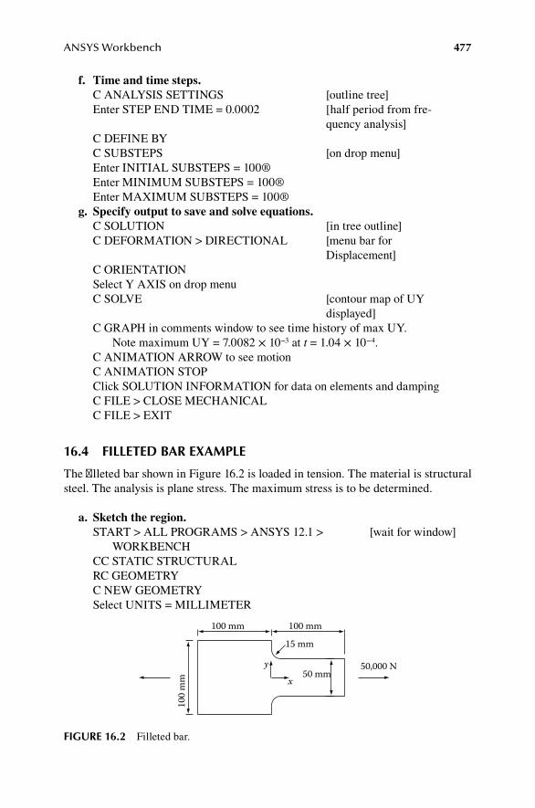
ANSYS Workbench 477
f. Time and time steps.C ANALYSIS SETTINGS [outline tree]Enter STEP END TIME = 0.0002 [half period from fre-
quency analysis]C DEFINE BYC SUBSTEPS [on drop menu]Enter INITIAL SUBSTEPS = 100®Enter MINIMUM SUBSTEPS = 100®Enter MAXIMUM SUBSTEPS = 100®
g. Specify output to save and solve equations.C SOLUTION [in tree outline]C DEFORMATION > DIRECTIONAL [menu bar for
Displacement]C ORIENTATIONSelect Y AXIS on drop menuC SOLVE [contour map of UY
displayed]C GRAPH in comments window to see time history of max UY. Note maximum UY = 7.0082 × 10⁻³ at t = 1.04 × 10−4.C ANIMATION ARROW to see motionC ANIMATION STOPClick SOLUTION INFORMATION for data on elements and dampingC FILE > CLOSE MECHANICALC FILE > EXIT
16.4 fIlleted Bar exaMple
The filleted bar shown in Figure 16.2 is loaded in tension. The material is structural steel. The analysis is plane stress. The maximum stress is to be determined.
a. Sketch the region.START > ALL PROGRAMS > ANSYS 12.1 > [wait for window] WORKBENCHCC STATIC STRUCTURALRC GEOMETRYC NEW GEOMETRYSelect UNITS = MILLIMETER
50,000 N50 mm
15 mm
100 mm100 mm
100
mm
y
x
fIgure 16.2 Filleted bar.

478 The Finite Element Method for Mechanics of Solids with ANSYS Applications
C OKC SKETCHING [left side below tree outline]C LOOK AT FACE PLANE [right most logo on menu bar]C DRAW to get menu [sketching toolbox]C POLYLINEClick on approximate location of each of the eight corners of the object
(before fillets) in sequence. Do not click on the starting point again. Be sure that an H appears for horizontal lines and a V for vertical lines.
RC after the last corner to get a menu and then selectC CLOSED ENDC CONSTRAINTS [sketching toolbox]C EQUAL LENGTHC PAIRS OF LINES that are required to have equal length [repeat these two steps for
each pair, two pairs of hori-zontal lines and one pair of vertical lines]
C SYMMETRY [constraint menu]C X-AXIS [axis of symmetry]C a top and bottom pair of linesC DIMENSIONS to get menu [general is default]C on a line and the location for the [for each dimension] dimensionENTER dimensions in details menuC ZOOM TO FIT LOGO [if necessary]C DISPLAY [dimensions menu]C to deselect NAME and VALUE is [to display actual values] selected automaticallyC MODIFY [sketching toolbox]C FILLETEnter Radius = 15®C pairs of lines to create a fillets [C edge filter if necessary]C DIMENSIONS > RADIUSC on a fillet and drag dimension line [shows R = 15] normal to the fillet
b. Create a surface body.C CONCEPT > SURFACES [detail window appears]FROM SKETCHEnter THICKNESS = 10®EXPAND XY PLANE [click on the + next to x–y
plane in the tree]C SKETCH1C BASE OBJECT NOT SELECTED [Apply option appears]C APPLY [Base Object = 1 sketch]C GENERATE [lightning logo—body is then
shaded]

ANSYS Workbench 479
C FILE > CLOSE DESIGN MODELER [project schematic is visible]RC GEOMETRY [wait]C PROPERTIESSet ANALYSIS TYPE = 2D [on details menu]CLOSE PROPERTIES WINDOW
c. Apply loads and supports.CC MODEL [wait for Mechanical to start]C UNITSC mm,kg,NRC STATIC STRUCTURALC INSERTC FRICTIONLESS SUPPORTC EDGE SELECTION LOGOC LEFT EDGEC APPLY [details menu, tag appears]RC STATIC STRUCTURALC INSERTC FORCE [for uniformly distributed
load]C DEFINE BY [details menu]C COMPONENTS [vector drop menu]C X-COMPONENT to select itEnter MAGNITUDE = 50000®C RIGHT EDGEC Yellow area by GEOMETRY in details window if necessaryC APPLY [tag appears]C STATIC STRUCTURAL in Tree to see loads and supports [Rigid motion constraints
will be automatically added]
d. Specify the desired output.RC SOLUTION [in tree outline]C INSERTC STRESS > MAXIMUM PRINCIPAL
e. Mesh the body.C MESH in the tree outline to highlight itC MESH CONTROL > SIZINGC on bodyC APPLY on geometry detailC ELEMENT SIZEEnter 10® [in place of “default”]C MESH CONTROL > METHOD [menu bar]C ANYWHERE ON THE BODYC APPLY on geometry detail [geometry = 1 body]C METHOD [details menu]

480 The Finite Element Method for Mechanics of Solids with ANSYS Applications
Select TRIANGLES from drop menu [tree shows “All Triangles Method”]
RC ALL TRIANGLES METHOD [in tree]C GENERATE MESHC MESH [too see mesh]EXPAND SATISTICS to see the number of elements
f. Solve and view results.C SOLVE [lightning logo on
menu bar][Note warning that rigid motion has been prevented by weak springs]C MAXIMUM PRINCIPAL STRESS [in solve tree to see
contour plot][Note maximum is σ1 = 147 MPa on fillet][Use BOX ZOOM to expand the region of high stress and Probe if desired]FILE > CLOSE MECHANICALFILE > EXIT
16.5 Sheet WIth a hole
A sheet with a central hole (Figure 16.3) is stretched by a uniform edge stress S resulting in a stress concentration at the hole. Symmetry is used so that only the upper-right quadrant is retained. This demonstrates automatic mesh refinement to improve result. In any convenient system of units: S = 100, a = 20, b = 10, r = 5, structural steel. The stress concentration is sought.
a. Sketch the region.START > ALL PROGRAMS > ANSYS 12.1 > [wait for window]WORKBENCHCC STATIC STRUCTURALCC GEOMETRY [to start Design
Modeler]Select UNITS = MILLIMETER [or your choice]C OK
Sxr
y
2a
2b
fIgure 16.3 Sheet with a hole.

ANSYS Workbench 481
C SKETCHING [left side below tree outline]C LOOK AT FACE PLANE [right most logo on menu
bar]C DRAW to get menu [sketching toolbox]C RECTANGLEClick on the origin and the approximate location of the upper right cornerC CIRCLEC the origin and the approximate location of a point on the circleC DIMENSIONS [to get menu, General is
selected]C top edge and location for dimensionC right edge and location for dimensionC RADIUSC on circle and location for dimensionEnter dimensions in the Details ViewC MODIFYC TRIM > IGNORE AXISClick on each line segment (circle and two enclosed line segments) to trim away [we now have the upper-
right quadrant sketched]b. Create a surface body.
C CONCEPT > SURFACES FROM [detail window appears]SKETCHEnter THICKNESS = 1® [arbitrary choice (area = 10)]EXPAND XYPLANE [click on the + next to x–y
plane in the tree]C SKETCH1C APPLY [first click yellow region if
necessary]C GENERATE [body is then shaded]C FILE > CLOSE DESIGN MODELER [project schematic is visible]RC GEOMETRY [WAIT]C PROPERTIESSet ANALYSIS TYPE = 2D [on pull down menu]CLOSE PROPERTIES WINDOW [X in upper right corner]
c. Apply loads and supports.CC MODEL [Wait for the model to
appear]]C UNITS [choose mm,kg,N, or your
choice]C STATIC STRUCTURALC SUPPORTS > FRICTIONLESS [menu bar] SUPPORTC EDGE SELECTION LOGO [menu bar]C LEFT EDGEC APPLY [tag appears]
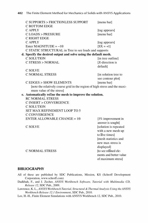
482 The Finite Element Method for Mechanics of Solids with ANSYS Applications
C SUPPORTS > FRICTIONLESS SUPPORT [menu bar]C BOTTOM EDGEC APPLY [tag appears]C LOADS > PRESSURE [menu bar]C RIGHT EDGEC APPLY [tag appears]Enter MAGNITUDE = −1® [SX = +1]C STATIC STRUCTURAL in Tree to see loads and supports
d. Specify the desired output and solve using the default mesh.C SOLUTION [in tree outline]C STRESS > NORMAL [X-direction is
default]C SOLVEC NORMAL STRESS [in solution tree to
see contour plot]C EDGES > SHOW ELEMENTS [menu bar] [note the relatively coarse grid in the region of high stress and the maxi-
mum value of the stress]e. Automatically refine the mesh to improve the solution.
RC NORMAL STRESSC INSERT > CONVERGENCEC SOLUTIONSET MAX REFINEMENT LOOP TO 5C CONVERGENCEENTER ALLOWABLE CHANGE = 1® [1% improvement in
answer is sought]C SOLVE [solution is repeated
with a new mesh up to five times]
[mesh statistics and new max stress is displayed]
C NORMAL STRESS [to see refined ele-ments and better value of maximum stress]
BIBlIography
All of these are published by SDC Publications, Mission, KS (Schroff Development Corporation, www . schroff.com)
Dadkhah, F., and J. Zecher, ANSYS Workbench Software, Tutorial with Multimedia CD, Release 12, SDC Pub., 2009.
Lawrence, K. L., ANSYS Workbench Tutorial, Structural & Thermal Analysis Using the ANSYS Workbench Release 12.1 Environment, SDC Pub., 2010.
Lee, H.-H., Finite Element Simulations with ANSYS Workbench 12, SDC Pub., 2010.

K12048_cover.fhmx 7/25/11 3:11 PM Page 1
C M Y CM MY CY CMY K
ELLIS H. DILL
The Finite ElementMethod for Mechanicsof Solids withANSYS Applications
The Finite Element Method for Mechanicsof Solids with ANSYS Applications
K12048
6000 Broken Sound Parkway, NWSuite 300, Boca Raton, FL 33487711 Third AvenueNew York, NY 100172 Park Square, Milton ParkAbingdon, Oxon OX14 4RN, UK
an informa business
The Finite Element Method for Mechanicsof Solids with ANSYS Applications
DILL
While the finite element method (FEM) has become the standard technique used to solvestatic and dynamic problems associated with structures and machines, ANSYS softwarehas developed into the engineer’s software of choice to model and numerically solvethose problems.An invaluable tool to help engineers master and optimize analysis, The Finite ElementMethod for Mechanics of Solids with ANSYS Applications explains the foundations of FEMin detail, enabling engineers to use it properly to analyze stress and interpret the outputof a finite element computer program such as ANSYS.Illustrating presented theory with a wealth of practical examples, this book covers topicsincluding
• Essential background on solid mechanics (including small- and large-deformationelasticity, plasticity, viscoelasticity) and mathematics
• Advanced finite element theory and associated fundamentals, with examples• Use of ANSYS to derive solutions for problems that deal with vibration, wave
propagation, fracture mechanics, plates and shells, and contact
Totally self-contained, this text presents step-by-step instructions on how to use ANSYSParametric Design Language (APDL) and the ANSYS Workbench to solve problemsinvolving static/dynamic structural analysis (both linear and nonlinear) and heat transfer,among other areas. It will quickly become a welcome addition to any engineering library,equally useful to students and experienced engineers.
Mechanical Engineering
ELLIS H. DILL


![Mechanics of Solids [3 1 0 4] CIE 101 / 102 First Year B.E ...icasfiles.com/mechanics of solids/notes/slides/1... · Mechanics of Solids PART-I PART-II Mechanics of Deformable Bodies](https://img.dokumen.tips/doc/110x75/60e4e466746b7501e128b225/mechanics-of-solids-3-1-0-4-cie-101-102-first-year-be-of-solidsnotesslides1.jpg)