Embed Size (px)
Citation preview
Pergamon
PII:S0360-1285(9"/)00025-7
Prog. Energy Combust. SoL Vol, 24, pp. 89-124, 1998 © 1998 El~vier Science Ltd
Printed in Great Britain. All rights re . f red 0360-1285/98 $19.00
THE FAST-RESPONSE FLAME IONIZATION DETECTOR
Wai K. Cheng *t, Tim Summers* and Nick Collings* *Sloan Automotive Lab, Massachusetts Institute of Technology, Cambridge, MA 02139, U.S.A.
*Engineering Department, Cambridge University, Cambridge CB2 IPZ, U.K.
Abstract--The fast-response flame ionization detector has become a widely used instrument for time-resolved hydrocarbon measurements in internal combustion engines. The characteristics of and working experience with the instrument are reviewed. In particular, the sampling system and its performance for isolating the pressure pulsation in in-cylinder and in engine exhaust measurements are described. Results from different applications are given to illustrate the utilities of the instrument. © 1998 Elsevier Science Ltd. All rights reserved.
Keywnrds: hydrocarbon, emissions, instrumentation, engine.
CONTENTS
I. Introduction 89 2. The Flame lonization Detector 90
2.1. Detector Characteristics: Linearity, Dynamic Range, Response Time 90 2.2. Response to Different Compounds 91 2.3. Oxygen Interference 92
3. The Fast-Response Flame Ionization Detector 93 3.1. Origins 93 3.2. Development for Automotive Use 93 3.3. Operating Principle of Sampling System 93 3.4. Deviations from Ideal Behavior 94 3.5. Sampling system performance 96
3.5.1. Transit time 96 3.5.2. Time constant 99
4. Working Experience with the Fast-Response Flame Ionization Detector 101 4. I. Pressure Fluctuation Isolation 101 4.2. Condensation Problems 102 4.3. Calibration 103
4.3.1. Calibration techniques 105 4.4. Typical FFID Setting 106 4.5. FFID Signal Compensation 106 4.6. In-cylinder Sampling at High Engine Speeds 106
5. Measurements with the FFID 108 5.1. Intake Flow Measurements 108
5.1.1. Capturing the intake flow processes 108 5.1.2. Measurement in intake manifold with port-fuel injection 109
5.2. In-cylinder Measurements 111 5.2.1. In-cylinder measurement of air/fuel ratio 112 5.2.2. Measurement of residual gas fraction 114 5.2.3. Study of in-cylinder HC sources 115
5.3. Exhaust Measurements in Spark Ignition Engines 116 5.3.1. Nature of the FFID signal in exhaust sampling 117 5.3.2. Calculation of HC emissions per cycle from the FFID signal in exhaust sampling 118 5.3.3. Examples of exhaust flow FFID measurements 119
5.4. Diesel Exhaust Measurements Using the FFID 121 6. Concluding Remarks 122 7. Acknowledgments 122 Nomenclature 122 References 122 Appendix A 123 Appendix B 124
I. INTRODUCTION
The fast-response flame ionization detector (FFID) was developed in response to the demand for time- resolved hydrocarbon (HC) measurements in internal
*Corresponding author: 31-165, MIT, Cambridge, MA 02139, U.S.A.
combustion engine research. This demand is motivated by the emissions regulations that require substantial reduction in passenger ears HC emissions; for example, by the US Federal Tier I and Tier II Standards and by the California Air Resources Board series of Low Emissions Vehicles standards (from Transition Low Emissions to Ultra Low Emissions)) To achieve low HC emissions, fundamental understanding of the HC
89
90 W.K. Cheng et al.
emission mechanisms is needed. The FFID facilitates this understanding by providing two types of informa- tion: crank angle-resolved data within one engine cycle to elucidate the detailed HC mechanisms in the engine process, and cycle-resolved data which connect the emissions to the overall engine operation. Examples of the latter are the assessment of the mixture preparation process in which the current cycle event is influenced by the events of the previous cycles, and the evaluation of catalyst performance in warm-up and in acceleration/ deceleration transients.
Over the past decade, the FFID has matured from a laboratory research item to a standard instrument for engine research and development. It was developed from a conventional flame ionization detector; the major innovation was the creation of a sampling system which isolates the pressure fluctuation at the sampling point so that there is a constant mass flow of the sampled gas into the detector. With appropriate sizing of the flow components, a response time of the order of a millisecond can be achieved. This response is in contrast to the conventional device which typically has a response time of the order of a second.
In this review, the principle and properties of the basic flame ionization detector are summarized first. Then the sampling system which is crucial to the FFID and its performance are described. Finally practical working experience with the instrument and application examples are given. The purpose of this review is to give a tutorial on the FFID so that users can obtain a comprehensive understanding of the instrument and assess its performance and limitations.*
2. THE FLAME IONIZATION DETECTOR
The flame ionization detector (FID) has been widely used for detecting hydrocarbons since the early 1960s. An excellent review of the behavior of the detector can be found in Ref. 2. In the following, the pertinent properties of the detector are briefly reviewed in connection to the FFID.
2.1. Detector Characteristics: Linearity, Dynamic Range, Response Time
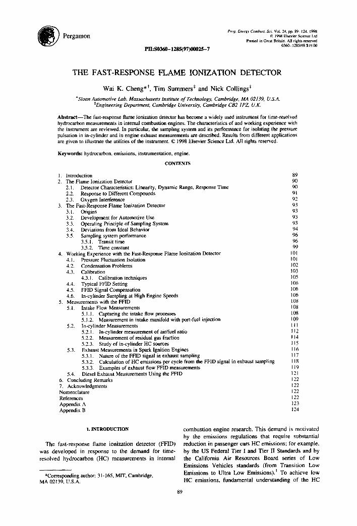
The first successful quantitative flame ionization detector was built by McWilliam and Dewar 3 for measuring the eluted hydrocarbons in gas chromatography. (The FID is still the predominant detector for gas chromatography.) The basic design (Fig. 1 (a)) has not changed over the years (although the
* It should be noted that this article is virtually entirely con- cerned with the FFID instrument manufactured by Cambustion Ltd. Other instruments are available with nearly comparable reponse times. However, the overwhelming majority of the work done to date with FFID has used this instrOment, and many of the application issues are common to all fast systems based around the sampling principle.
McWilliam and Dewar detector used two FIDs in a differential arrangement). A diffusion flame is established with hydrogen (sometimes diluted with helium or nitrogen) as the fuel in a slow co-flowing air stream. Typical burner 2 ID is - 0 . 5 mm with a fuel flow velocity of - 1 0 m s -l and an air flow velocity of 0.05 m s -t, the flow is laminar (the jet Reynolds number is below 50- - the value depends on the operating pressure). There is negligible ionization in the flame until hydrocarbon species are introduced. The flame ions are collected by an electrode negatively biased at 150- 200 volts with respect to the burner and located at - 1 cm above the burner.
The ion pair production process is complex. It is generally accepted 2'4-6 that thermal ionization is negligible in such flames and the charge production is a chemi-ionization process involving reactions such as
C H + O ~ CHO + + e - (1)
The overall reaction is approximately thermally neutral. 5
The yield is ~2.5 × 10 -6 ion/electron pairs per aliphatic
carbon atom, or 0.245coulombs/g-atomC. 2'7 (The
response to various hydrocarbon molecules will be
discussed in the next section.) The positive ions change
- 1 8 0 V
A i r
10 2
+T
Charge Collector
~ _ Hydrogen FF --'1--~ Sample flow
(a)
. . . . . . . '1 . . . . . . . . I . . . . . . . . I . . . . . . . . I . . . . . . ~.
10
.-= ! tt)
10.1
6O
10"2
i , i i l l t i l i , t l i l l i l i , i l t l i , [ I l l i l l i i l I i } i l
10"10.9 10-8 10-7 10-6 10-5 10-4
Sample introduction rate (g-atom C/s)
(b)
Fig. 1. (a) A typical flame ionization detector; (b) linearity of FID output using propane as the test hydrocarbon. 2 The
deviation from Eq. (4) is within __. 1.5%.
The fast-response flame ionization detector 91
identity constantly, particularly by proton transfer, and
the process creates a complex ion spectrum. The
recombination is dominated through the hydronium
ion, H3 O+ which results from charge transfer processes made favorable by the large amount of water vapor
present:
CHO + + H 2 0 - ' * H 3 O+ + C O (2)
H3 O+ -k-e- ---, 2H + O H (3)
If all the charges are collected by the electrode, then for a
hydrocarbon with molecular formula CnHm, the current
collected by the electrode, i(A), is given by:
i = r[CnH,,]Q (4)
where [C,H,,,] is the molar concentration (mol cm3-~),
and Q is the sample volume flow rate (cm 3 s -1) through
the detector. For aliphatic hydrocarbons, the response
function, r, is proportional to n, the number of carbon
atoms in the molecule:
r = tun (5)
The proportional constant is ot = 0.245 coulombs/
g-atom C. The linearity of the instrument to the HC mole
concentration given by Eq. (4) depends on the assump- tion that all (or a fixed fraction) of the charge is captured by the electrode. In reality the charge collection process is in competition with the recombination process. Charge collection is incomplete at high fuel jet velocities at which charges are blown out of the high electric field region, or at high charge density when the electric field cannot effectively penetrate the space between the electrodes and the charge collection process is impeded.
Another possible cause of non-linearity is charge multiplication if the electric field is too high. For typical collector geometry with sharp edges avoided, there is negligible electron multiplication when the bias voltage is under 200 V.
Good linearity over an extensive range can be achieved with a properly designed FID. For example, the data in Fig. l(b) for propane have a scatter within -+ 1.5% over four decades. The noise current in a clean
hydrogen flame is predominantly due to the shot noise associated with background ionization. For the particular detector 2 used in generating the data in Fig. l(b), the noise current is -10-14 A xHz-l. Using this figure, the lower limit of detection (at twice the noise level and at 1 kHz bandwidth) would be at - 6 × 10 -13 A. Using the highest point of Fig. 1 (at - 16 .uA) as the upper limit, the dynamic range of the detector is of the order of 1 0 7 .
Further linearity tests with different compounds as the test gas are listed in Ref. 2. Of course linearity suffers if the sample flow becomes a significant proportion of the fuel f low--a maximum sample flow rate of --3% of the fuel flow was suggested in that reference.
The response time of the FID to a HC sample depends on the following processes:
1. diffusion during the flow time of the HC to the reaction zone of the flame;
2. kinetics of the cracking of HC into fragments of reactive species such as CH, CH2 etc.;
3. kinetics of the chemi-ionization process such as Eq. (1);
4. charge transport time; 5. charge amplifier bandwidth, which may be
suppressed to reduce noise. Added to the above is the sampling system transport
time, which will be discussed in a later section. For most applications, (5) is not a limiting factor. Rate estimates for processes (2), 7 (3) 8 and (4) 6 can be made, though the chemistry is very fast. The precise values, however, depend much on the operating conditions: HC concen- tration, pressure, temperature, details of the mixing rate of the diffusion flame, geometry of the electric field, etc. In practice, the response time of a well designed FID (excluding the sampling system) is well below 1 ms.
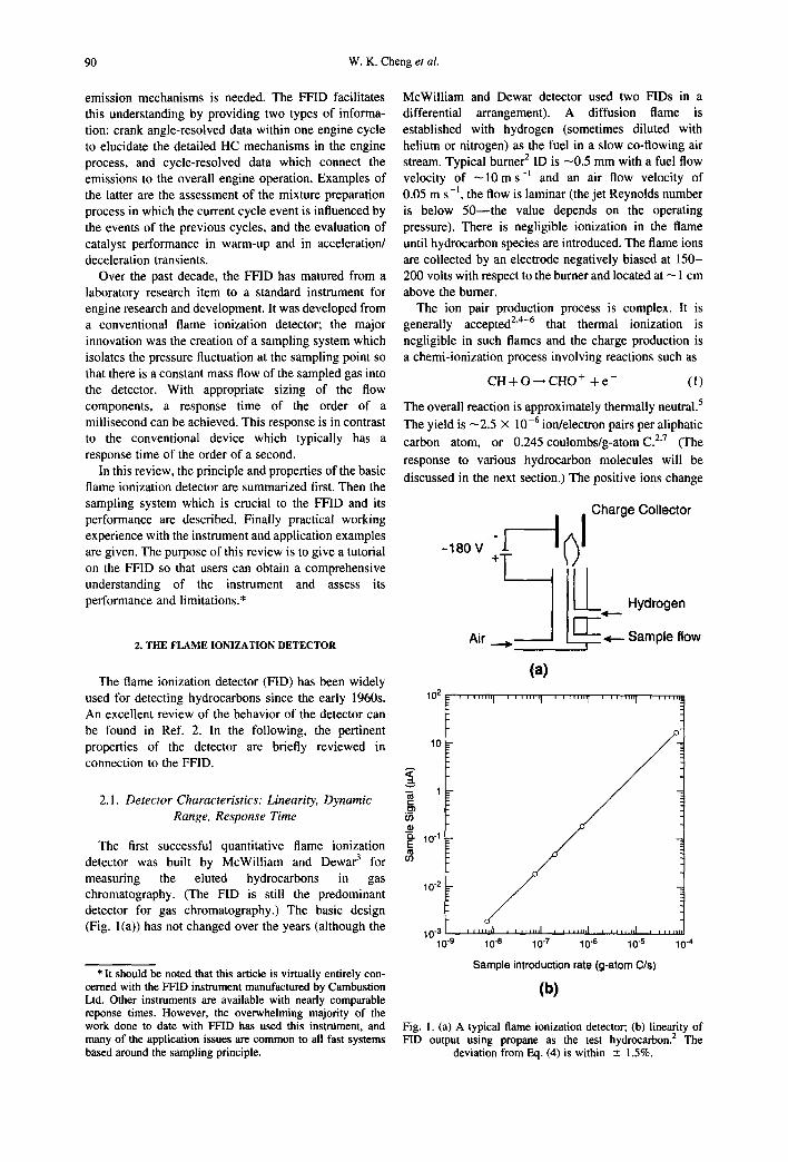
2.2. Response to Different Compounds
The response of the FID to different compounds was researched extensively. 2'9 ~ The response functions, r, defined in Eq. (4) and normalized by defining the value for n-heptane --- 7, for alkanes, cyclo-alkanes, alkenes, alkynes and aromatics are shown in Fig. 2. The remarkable proportionality of the response to the number of C atoms in each molecule in these families of compounds (with the exception of acetylene, which has a response of --30% higher), and the linearity of the instrument (see Fig. 1 ) lead to the general conception that the FID is a carbon counting device for hydrocarbons.
The response function for other carbon containing
1 2 4 ' ' ' 1 . . . . I . . . . I . . . . i , , , , i , , r-~
t 0 © Alkanes <> Cyclo-alkanes
a ® Alkenes [] Alkynes
"5 8 A Aromatics
° ( ~ 6
> / 4 / 6
-_/U
0 2 4 6 8 10 12
No. of C atoms in molecule
Fig. 2. Relative FID response of alkanes, cyclo-alkanes, alkenes, alkynes, and aromatics (response of n-heptane ----= 7). Data listed
2 9 1 0 in Appendix A. ' ' Dashed line represents y values = x values.
/ /
92 W.K. Cheng et aL
compounds are different. It is well known that the FID does not respond to carbonyl carbons. For example, CO2 and CO produce negligible ionization. The carbonyl carbons in aldehydes, ketones and esters behave similarly (Fig. 3). A proposed explanation 2 is that it is ' the exothermic reactions associated with the formation of the carbon-oxygen bond from reduced forms of carbon that provide the high energy states which may lead to ionization. Where a carbon is already oxidized in the starting sample, an oxidized carbon fragment is split out in the endothermic cracking stage of the reactions, and this oxidized carbon fragment is incapable of producing ionization in the flame.' The data on ether (Fig. 3) further support this explanation, since the bond
~ ' ' ' ' I ' ' ' ' I ' ' ' ' I ' ' ' ' I ' ' ' ' I/~/~
1 0 ~ A Esters / . ~ ¢ Aldehydes and ketones / A¢"
f II Ethers / / ~ / "~ 8 / / " .
/ / .m >~
o V L , x , h , , , I ~ , , , I , , , , I . . . . I , , 0 2 4 6 8 10
No. of C atoms in molecule
Fig. 3. Relative FID response of esters, aldehydes and ketones, and ethers (response of n-heptane --= 7). Data listed in Appendix A. 2'9 Dashed line represents y values = x values - I.
10, . . . . I . . . . I . . . . I . . . . I ' ' ' ~ / 1
o primary alcohols / . / ~ • Secondary alcohols / / /
8 ~ Terti a ,'7
• 6 u) c- O
u) .= • 4 ._>
2
0 / , , , I . . . . I , , t ~ l n , L J l ~ , , ~ 0 2 4 6 8 10
NO. of C atoms in molecule
Fig. 4. Relative FID response of alcohols (response of n-heptane --- 7). Data listed in Appendix A. 2'° Dashed line represents y
values = x values - 1/2.
rupture process tends to leave the O in the ether in one of the C atoms.
For alcohols, the C bonded to O in the R - O - H group (R stands for an alkyl) contributes to a FID response of a fraction of a C atom (Fig. 4). The fractional contribution may be attributed to whether the bond rupture process is dehydrogenation (removal of H) or dehydration (removal of OH); the former would not contribute to the production of ions. The difference in response between the primary, secondary and tertiary alcohols supports this explanation: the secondary alcohols, which are most easily dehydrogenated into carbonyl com- pounds show the lowest response. The tertiary alcohols, which are most easily dehydrated, show the highest response. The primary alcohols are in between.
The contributions to the FID response effective carbon number for the various bonds are summarized in Table 1.
2.3. Oxygen Interference
When the sample flow contains oxygen, there are changes in the flame temperature, in the geometry of the flame, in the geometry of the ion generation region, and in the competition between formation of flame ions and oxidation of the hydrocarbon fragments. As a result, the FID signal is sensitive to the sample flow oxygen content, which usually leads to a decrease of the response function. (This effect is often termed oxygen synergism.)
The oxygen interference on the FID signal 2A2 depends on the details of the FID design and operating conditions: the operating pressure; the fuel flow rate; the amount of diluent in the fuel (hydrogen) flow. Typical examples are shown in Figs 5 and 6. The errors introduced because of oxygen synergism are significantly reduced by the use of a fuel gas consisting of a helium/hydrogen mixture (typically 60/40 mix), and this is almost universally used in the traditional 'slow' instruments. The operating range of the FFID, however, can be enhanced significantly by the use of pure hydrogen as the fuel gas.
In automotive applications, there is a substantial difference in the oxygen content of the burned and unburned gas. In practice, the FID is a calibrated
Table 1. Effective carbon number contribution to FID response 2
Atom Bonding type Effective contribution to C No.
C Aliphbatic 1.0 C Aromatic 1.0 C Olefinic 0.95 C Carbonyl 0.0 C Nitrile 0.3 O Ether - 1.0 O Primary alcohol -0.6 O Secondary alcohol -0.75 O Tertiary alcohol -0.25 CI Two or more single -0.12 each
aliphatic C CI On olefinic C +0.05 N In amines Similar to O in
corresponding alcohols
The fast-response flame ionization detector 93
1.0
o.sJ t- ~ 0.6
LL 0 . 4 - -
0.2
' I ' ' ' = I . . . . I ' ' "
/ /
- - no 0 2 in samp le gas - - - - - 4 cc /min 0 2 in samp le gas
o , , L J I , , J , I J , , , I , , 0 20 40 60
H y d r o g e n f l o w ra te ( c c / m i n )
Fig. 5. Sample flow oxygen effect on FID response. 2 Fixed sample of 4.13 x 10 -8 mol s -~ of n-heptane in an argon carder of 60cmJmin-~; air flow of 800cmtmin-~; various fuel (hydrogen) flow rates. Y axis normalized so that peak of the
solid curve is unity.
o~ a i O~ 0 t -
e- c- I:~ -8 x 0 9. ~ -12 -i 121
~ -16
m -20
-24 0
==
-rcr ~ ~ ~ Xi._~ "~ 14.6 4.0
7.7
_ ~ x o 4 . 6 12.7
\ , . . "b 2 9 . 2 2 O
. . . . I . . . . I . . . . I . . . . I , , , , t ' . , , ,
2 4 6 8 10
O x y g e n C o n c e n t r a t i o n in S a m p l e , V o l . %
12
Fig. 6. The effect of oxygen concentration and analyzer operating conditions on oxygen interferenceJ 2 (Perkin-Elmer flame-ionization analyzer; airflow rate: 175 ml min-~; fuel: hydrogen, fuel flow rate 6-38 ml min-I; sample: 100, 303 and 1010 ppm n-hexane in nitrogen diluted with various amounts of
oxygen; sample flow rate 3 ml min-~.)
instrument, and the span gas used for calibration thus depends on the application. For burned gas measure- ment, the span gas used is typically a propane/nitrogen mixture of known composition. For unburned gas measurement, the span gas used is typically a propane/ air mixture. Although the ratio of oxygen to nitrogen in air may not match that of the oxygen to inert (nitrogen
plus the residual gas, which is often present) in the unburned gas, the difference is usually overlooked because the proportion of residual gas in the unburned mixture is often not known. For measurements involving a mixture of burned and unburned gases, there could be substantial uncertainty because an educated guess (or an independent measurement) must be made of the oxygen concentration, and the instrument needs to be calibrated at different sample gas oxygen levels.
3. THE FAST-RESPONSE FLAME IONIZATION DETECTOR
3.1. Origins
The first fast-response flame ionization detector (FFID) was described in a article by FackrellJ 3 who modified a standard FID in order to study rapid concentration fluctuations (using methane or propane as tracer) in a (essentially constant pressure) wind tunnel experiment. Automotive applications such as measure- ments of the HC in the exhaust ]4 and in-cylinder ]5 were first done at Cambridge University in the late 1980s. A commercial instrument, based on the Cambridge work appeared in production in 1990. The instrument has since been used in a wide range of automotive applications.
3.2. Development for Automotive Use
Crucial to the automotive use of the FFID is its sampling system. Unlike the traditional 'quasi-steady' FID design in which the sample flow is premixed with the fuel, the sample is drawn directly into the flame without mixing with the fuel so as to minimize mixing processes deleterious to good frequency response, and to minimize the sample transit time. An important con- sideration is that the signal from the FID is proportional to both the HC concentration and the sample flow rate (see Eq. (4)). Therefore for meaningful interpretation of the signal in terms of HC concentration, a constant sample flow rate is required. In most automotive applications, however, the sample inlet is exposed to a fluctuating pressure; for example when sampling from the exhaust or from the cylinder of an SI engine. In the former, pressures may fluctuate by significant fractions of a bar, in the latter, from 0.5 bar to over 50 bar. If a sampling tube were to be connected directly to FID, the sample flow rate would have varied significantly. Therefore an effective pressure isolation system is essential to the successful operation of the FFID.
In the following, the operating principle of the sampling system is first described. The system behavior in terms of the transit time and the sample dispersion which determines the frequency response of the instrument are then discussed.
3.3. Operating Principle of the Sampling System
A method to provide a constant mass flow to the FID is the use of a constant pressure chamber between the
94 W.K. Cheng et al.
VACUUM
BLEED TYPICAL DIMENSIONS (ram) FLOW Length Diameter
(A)Transfer tube 100 0.2 (B)Settling tube 25 0.8 (C)Connecting tube 30 0.15 (D)Ballast chamber Volume ~ lcc
Fig. 7. Sampling system of FFID, as applied to in-cylinder sampling in an IC engine. =7
sampling inlet and the FID detector itselfJ 6 The configuration is shown in Fig. 7. Referring to the figure, a sample is drawn through a small diameter Transfer Tube A which is connected to a larger tube (the Settling Tube B*) that terminates in the Ballast Chamber D, which is usually held at a significant (and constant) vacuum level below ambient. The ballast chamber acts as a capacitor, which, together with the resistance of the tubes A and B, maintains a very nearly constant pressure at D, despite flow changes due to sample pressure changes. Thus the chamber D is often referred to as the Constant-Pressure (CP) Chamber. The sample to the FID is taken at the end of the Settling Tube B in a 'T ' arrangement by the Connecting Tube C, which delivers the HC sample directly to the hydrogen flame in the FID. The principle is to maintain a constant pressure across tube C so that a constant flow rate is delivered to the FID.
The FID detector receives, via tube C, a sample of the flow in the Transfer Tube, i.e. it receives a sample of the sample flow entering the sampling system, and most of the total sample flow discharges into the CP chamber. The 'tee' arrangement at inlet to tube C (the 'FID' tube), is designed as a variation on the principle of a static pressure tapping, (that is a tapping which indicates the static pressure independent of the velocity of the gas crossing the face of the tapping). In the situation here, a small flow, the FID sample, is allowed along the tube; the pressure gradient associated with the stream line curvature of this small entrance flow is negligible. The pressure at entry to the FID tube is thus constant because the pressure there is independent of the flow velocity across it, and because the streamlines exiting into the CP chamber are parallel. The only difference will be caused by the very small amount of friction pressure drop in the
* In earlier papers, the Seuling Tube has been referred to as the Expansion tube, which is a misnomer. The cross-section of the jet flow from the Transfer Tube exit expands, but thermodynamically, the process is the reverse of expansion.
short length of tube approximately 1 mm, between the FID tube tapping and exit into the CP chamber.
The only situation in which the pervious arguments will be in error is when the exit flow into the CP chamber becomes choked, in which case the pressure in the CP chamber and that at entry to the FID tube may be very different. This is why the Settling length B is included-- it ensures that if choking occurs it will be at the exit of tube A, and that the FID inlet remains at CP pressure.
The average pressures in the CP chamber and the FID chamber are maintained by a system of bleed flow and vacuum lines. Typically a differential pressure regulator is used to keep the pressure difference across the Connecting Tube C constant. The practical arrangement will be discussed in Section 4.
3.4. Deviations f rom Ideal Behavior
While the DC level of the CP chamber is maintained by the bleed and vacuum flow system, the pressure fluctuation caused by the variation of the Transfer Tube mass flow over an engine cycle is damped by the first order filtering of the (non-linear) Transfer Tube flow resistance and the capacitance of the CP chamber volume. It should be noted that though the ballast chamber volume as drawn in Fig. 7 is quite small (--1 cm3), the effective volume for the CP chamber is very substantially larger due to the volume of the vacuum lines and the other pressure regulating devices. (For example, a 5 mm ID line of l m length adds - 2 0 c m 3 to the volume.) For a typical system, the effective CP chamber volume is ~ 100 cm 3 or larger.
To calculate the damping factor caused by the transfer line and the CP chamber, quasi-steady isothermal flow in the tube is assumed. (For the capillaries used, isothermal flow is an excellent approximation, except very close to the exit of the Transfer Tube if the flow is choked, or very nearly so.) Then for an inlet pressure of Pi, mass
The fast-response flame ionization detector 95
flow rate rh in the Transfer Tube isiS:
rn 2RT ~2(+--~-n pP_~i ) (6)
(See nomenclature section for definition of symbols.) If
the flow is choked, then the value of Pc in the above
formula is replaced by P*, the downstream choking
pressure. (The choking phenomenon will be discussed
and values of P* will be given in Section 3.5.) It
should be noted that Eq. (6) is implicit in th; this is
b e c a u s e f = f ( R e ) and the Reynolds number is given by
4rn Re = (7)
wd#
Note also that for an isothermal flow the viscosity # is
constant (since it is virtually only a function of temper-
ature), and thus in steady flow the values of Re and f a r e
constant along the tube. To estimate the variation in the
CP chamber pressure &Pc in one engine cycle, the
pressure pulsation at the sampling inlet may be repre-
sented by a triangular pulse of mass flow with the peak
value equal to the flow rate at the peak sample inlet
pressure and with duration equal to 1/4 of a (four stroke)
engine cycle. (In other applications, suitable other
criterion could be applied.) Then, for a CP chamber
volume V,
15 RT &Pc = R--~rhpc~k T - (8)
Values for ~Pc as a function of the sample inlet peak
pressure are shown in Fig. 8 for V = 100cm 3 and a
Transfer Tube of 0.2 mm diameter and I00 mm length.
1 0 . 2
r - o
o
~ 10.3 (D
Q .
E i -
~ 10-4 Laminar Turbulent
= t J l J l I I t ~ l l l I J L = i I
1 1 0 1 0 2
Variation of peak sample inlet pressure (bar)
Fig. 8. Estimated constant-pressure chamber pressure fluctua- tion as a function of sample inlet peak pressure variation; CP chamber volume = 100cm3; engine at 1000rpm; 0.2mm
diameter Transfer Tube of length 100 mm at 120 C.
Typical pressure difference between the CP chamber and
the FID is - 0 . I bar. To maintain a FID sample flow
variation of -< 1%, the value of &Pc should be - 1 x
10-3bar. Thus, according to Fig. 8, the system is
adequate for sampling in the exhaust and intake mani-
fold. For in-cylinder sampling, however, either the
volume of the CP chamber or the Transfer Tube flow
resistance has to be increased substantially. Equations (6)-(8) may be used to assess the scaling
relationship of the CP chamber pressure fluctuation, &Pc, to the system parameters. The friction factor for a smooth pipe* is given by:
f = 64~Re Laminar flow (9a)
f=O.316Re-1 /4 Turbulent flow (9b)
If the log term in Eq. (6) can be omitted, significant
simplifications result in the analysis. This term arises
from the difference in the inlet and outlet momentum,
and in most cases, this contribution to the pressure drop
along the capillary is much smaller than the friction term.
Only when the pressure ratio is very high, as in the case
of in-cylinder sampling, are the terms of comparable
magnitude. If then we ignore the In(Pi/Pc) term, we find from Eqs
(6)-(9a,b) that:
d 4 tSp c c< Laminar flow (10a)
V.L
d2.71 t3P c ~ V.LO.57 Turbulent flow (10b)
These equations may be used to scale the results in Fig. 8
to other system sizes. Equations (8) and (10a,b) were
verified by measuring the values of &Pc when different
diameter Transfer Tubes and different size ballast
chambers were used in the FFID. 19 The results are
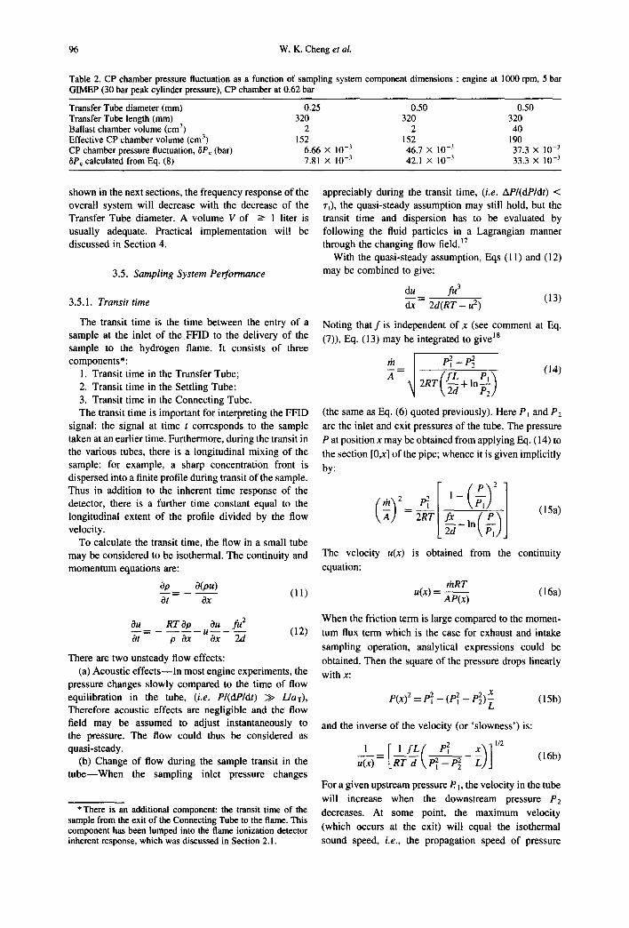
shown in Table 2. In Table 2, the 'parasitic' volume, which was added to
the ballast volume to form the effective CP volume, was calculated by comparing the &Pc values when the two different size ballast chambers were used; its value was 150 cm 3. When the tube diameter was increased by a factor of two, the ratio of &Pc was 46.7/6.66 = 7.0. This value compares favorably with the scaling of Eq. (10): 227~ = 6.54. Further, the values of &Pc calculated from Eq. (8) agree well with the observed values in spite of the simplicity of the model.
In practice, though the flow resistance is sensitive to the tube diameter, it is preferable to reduce the CP pressure variations by increasing V. This is because (a) it is difficult hardware-wise to use tubing of diameter much less than 0.2 mm, and more importantly, (b) as will be
* The roughness of the internal surface of typical tubes used in the FFID was measured to be ~ 1.4 #m. ~9 Therefore, for tube diameters of the order of a fraction of a ram, the smooth pipe correlation could be used up to Re~ 105.
96 W.K. Cheng et al.
Table 2. CP chamber pressure fluctuation as a function of sampling system component dimensions : engine at 1000 rpm, 5 bar GIMEP (30 bar peak cylinder pressure), CP chamber at 0.62 bar
Transfer Tube diameter (mm) Transfer Tube length (mm) Ballast chamber volume (cm 3) Effective CP chamber volume (cm 3) CP chamber pressure fluctuation, 6Pc (bar) ~SP c calculated from Eq. (8)
0.25 0.50 0.50 320 320 320
2 2 40 152 152 190
6.66 × 10 -3 46.7 × 10 -3 37.3 × 10 -3
7.81 × 10 -3 42.1 × 10 -3 33.3 X 10 -3
shown in the next sections, the frequency response of the overall system will decrease with the decrease of the Transfer Tube diameter. A volume V of ----- 1 liter is usually adequate. Practical implementation will be discussed in Section 4.
3.5. Sampling System Performance
3.5.1. Transit time
The transit time is the time between the entry of a sample at the inlet of the FFID to the delivery of the sample to the hydrogen flame. It consists of three components*:
1. Transit time in the Transfer Tube; 2. Transit time in the Settling Tube; 3. Transit time in the Connecting Tube. The transit time is important for interpreting the FFID
signal: the signal at time t corresponds to the sample taken at an earlier time. Furthermore, during the transit in the various tubes, there is a longitudinal mixing of the sample: for example, a sharp concentration front is dispersed into a finite profile during transit of the sample. Thus in addition to the inherent time response of the detector, there is a further time constant equal to the longitudinal extent of the profile divided by the flow velocity.
To calculate the transit time, the flow in a small tube may be considered to be isothermal. The continuity and momentum equations are:
~p O(ou) ,gt Ox (11)
Ou RT Op Ou fu 2 - - = u ( 1 2 ) Ot p Ox Ox 2d
There are two unsteady flow effects: (a) Acoustic effects--In most engine experiments, the
pressure changes slowly compared to the time of flow equilibration in the tube, (i.e. Pl(dPIdt) >> LlaT), Therefore acoustic effects are negligible and the flow field may be assumed to adjust instantaneously to the pressure. The flow could thus be considered as quasi-steady.
(b) Change of flow during the sample transit in the tube- -When the sampling inlet pressure changes
* There is an additional component: the transit time of the sample from the exit of the Connecting Tube to the flame. This component has been lumped into the flame ionization detector inherent response, which was discussed in Section 2.1.
appreciably during the transit time, (i.e. AP/(dPIdt) < rt), the quasi-steady assumption may still hold, but the transit time and dispersion has to be evaluated by following the fluid particles in a Lagrangian manner through the changing flow field. 17
With the quasi-steady assumption, Eqs (11) and (12) may be combined to give:
du fu 3 ~ = 2d(RT - u 2) (13)
Noting that f is independent of x (see comment at Eq. (7)), Eq. (13) may be integrated to give 18
A-- I 2 R T ( ~ d + l n ~ ) (14)
(the same as Eq. (6) quoted previously). Here Pi and P2 are the inlet and exit pressures of the tube. The pressure P at position x may be obtained from applying Eq. (14) to the section [0,x] of the pipe; whence it is given implicitly by:
(;) ( A ) ----2-~ f x - (15a)
The velocity u(x) is obtained from the continuity equation:
rnRT u(x) = (16a)
AP(x)
When the friction term is large compared to the momen- tum flux term which is the case for exhaust and intake sampling operation, analytical expressions could be obtained. Then the square of the pressure drops linearly with x:
X P(x) = - - Z
and the inverse of the velocity (or 'slowness') is:
u(x) = 2---- z Pt - P2
(15b)
(16b)
For a given upstream pressure P.i, the velocity in the tube will increase when the downstream pressure P2 decreases. At some point, the maximum velocity (which occurs at the exit) will equal the isothermal sound speed, i.e., the propagation speed of pressure
The fast-response flame ionization detector 97
wave under isothermal condition*. Then, according to
Eq. (13), du/dx will be infinite. The flow is said to be
choked: when P2 is decreased further, the flow field is
independent of the downstream pressure P2. The velocity
at the exit remains sonic (at the isothermal sound speed
aT) with a corresponding pressure P*. The flow adjusts to
the pressure P2 outside the tube. The value of P* as a function of P ~ may be calculated
from Eq. (14) by replacing P2 with P* and setting the mass flux equal to aT AP*IRT. The resulting equation is
(p , )2 (~**) fL (17a) ~-~ - 21n - l = - ~ -
Note that f is a function of rh, hence of P*, and the
equation has to be solved implicitly. The results are
shown in Fig. 9 for a tubing of diameter d = 0.2 mm,
at various L/d. Since the absolute value of d only enters
in the Reynolds number in evaluating f, and that when
the flow is choked, it is usually in the turbulent regime
w h e r e f ~ d TM, the result is not sensitive to the value ofd.
The value of P* is approximately proportional to PI. (It
would have be exactly proportional if f were not a func-
tion of Re. In the turbulent regime, the dependence is weak; f~Re -1/4.)
If the friction term dominates, Eq. (17) reduces to:
PI P* - (I 7b)
When choking occurs, the isothermal assumption cannot
hold, as it would require infinite heat transfer at the sonic
point. Nevertheless, for the majority part of the tubing (at
which the velocity is low, and which has the biggest
contribution to the transit time), the isothermal assump-
tion is still good. The flow field could thus be solved
from Eq. (14) with P* replacing the downstream
pressure P2. The error in mass flow when making the isothermal
approximation was assessed by a ID numerical simula- tion with finite heat transfer rate. E° There are three effects: the variation of the temperature along the tube; the difference between the adiabatic and isothermal criterion in choking; the use of isothermal rather than adiabatic sound speed in the evaluation of the choking point. The maximum mass flow error was found not to be significant (~ 1.5%).
When the FFID is used in exhaust or intake manifold sampling in a naturally aspirated engine, the sampling inlet pressure is low (approximately equal to or less than atmospheric) and the flow throughout the sampling system is usually unchoked. In in-cylinder sampling, however, the Transfer Tube will choke sometime in the
*Under isothermal condition, the sound speed aT is x(dp /dp)T =- x(RT). In normal sound propagation, the process is assumed to be isentropic; thus the normal sound speed is x(dp/dp)s = ~(~RT).
compression process. The relaxation of the Transfer Tube exit pressure P* to the CP chamber pressure Pc is complex. When P* is just slightly above Pc, the Settling Tube acts as a diffuser (not a very efficient one because of the step change in area from the Transfer Tube to the Settling Tube). At higher values of P*, the sonic jet may expand to be supersonic and relaxes to Pc through a series of shock diamonds or through a normal shock. 2j At very high sample inlet pressure, the Transfer Tube may become unchoked; instead the flow chokes at the exit of the settling chamber. In practice, this condition is usually avoided by choosing the size of the Settling Tube appropriately.
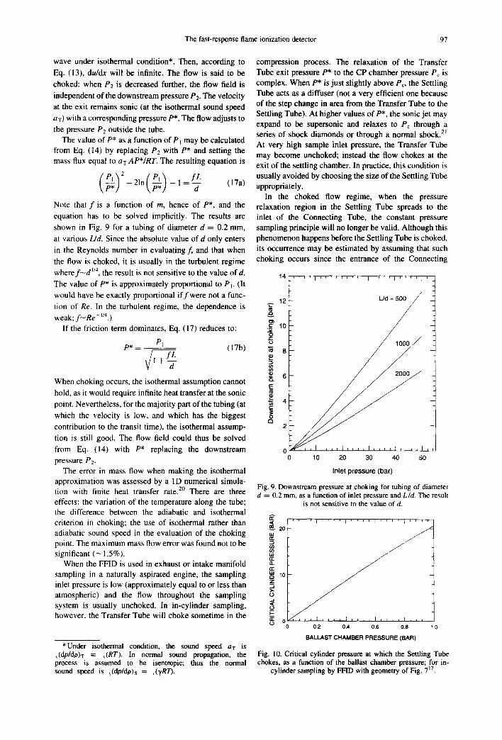
In the choked flow regime, when the pressure relaxation region in the Settling Tube spreads to the inlet of the Connecting Tube, the constant pressure sampling principle will no longer be valid. Although this phenomenon happens before the Settling Tube is choked, its occurrence may be estimated by assuming that such choking occurs since the entrance of the Connecting
. . . . I . . . . [ . . . . I . . . . I . . . . I
,.~m 12 L / d /
10
e~
-
~ 4
O
a 2
o . . . . . . . . . . . . . i 0 10 20 30 40 50
Inlet pressure (bar)
Fig. 9. Downstream pressure at choking for tubing of diameter d = 0.2 mm, as a function of inlet pressure and L/d. The result
is not sensitive to the value of d.
E" oO 20
8
O 0.2 0.4 0.6 0.8 1.0
BALLAST CHAMBER PRESSURE (BAR)
Fig. 10. Critical cylinder pressure at which the Settling Tube chokes, as a function of the ballast chamber pressure; for in-
cylinder sampling by FF[D with geometry of Fig. 717.
14
98 W.K. Cheng et al.
Tube is very close to the exit of the Settling Tube. Then Eq. (13) could be integrated backwards from the exit of the Settling Tube to the entrance of the Transfer Tube to obtain the critical cylinder pressure at which the Settling Tube becomes choked. The result is shown in Fig. 10 for the FFID geometry of Fig. 7. For example, the compression pressure just before ignition for a naturally aspirated engine at WOT is ~8 bar. Therefore if the ballast chamber pressure is above ~0.4 bar, choking at the Settling Tube would not occur until sometime into the combustion period.
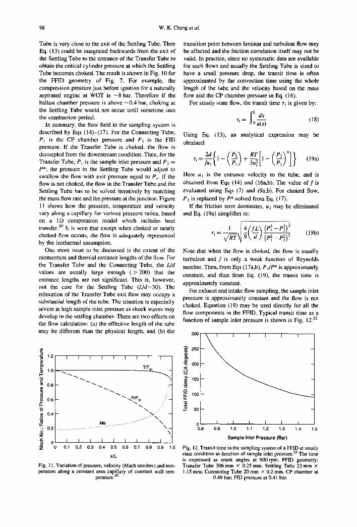
In summary, the flow field in the sampling system is described by Eqs (14)-(17). For the Connecting Tube, PI is the CP chamber pressure and P2 is the FID pressure. If the Transfer Tube is choked, the flow is decoupled from the downstream condition. Then, for the Transfer Tube, P~ is the sample inlet pressure and P2 = P*; the pressure in the Settling Tube would adjust to swallow the flow with exit pressure equal to PC. If the flow is not choked, the flow in the Transfer Tube and the Settling Tube has to be solved iteratively by matching the mass flow rate and the pressure at the junction. Figure 11 shows how the pressure, temperature and velocity vary along a capillary for various pressure ratios, based on a 1D computation model which includes heat transfer. 2° It is seen that except when choked or nearly choked flow occurs, the flow is adequately represented by the isothermal assumption.
One more issue to be discussed is the extent of the momentum and thermal entrance lengths of the flow. For the Transfer Tube and the Connecting Tube, the /-/d values are usually large enough ( > 200) that the entrance lengths are not significant. This is, however, not the case for the Settling Tube (L/d~30). The relaxation of the Transfer Tube exit flow may occupy a substantial length of the tube. The situation is especially severe at high sample inlet pressure as shock waves may develop in the settling chamber. There are two effects on the flow calculation: (a) the effective length of the tube may be different than the physical length, and (b) the
¢)
*~ 1.2
E 1.0 I-
t~ 0 ,8
~ 0,6
tn 0.4 o
r r "r 0.2 o Z
o
I f I I I I I I i
Trr~..........~
"~" ~ ~ "~" \ \ \ \P/Pin ::: ~ ' ~ . ...."'
. . . . , " " ~ Ma .......... \
I I I I I I I I I 0.1 0.2 0.3 0.4 0.5 0.6 0.7 0.8 0.9 1.0
x/L
Fig. 11. Variation of pressure, velocity (Mach number) and tem- perature along a constant area capillaz 3, of constant wall tem-
perature. 2°
transition point between laminar and turbulent flow may be affected and the friction correlation itself may not be valid. In practice, since no systematic data are available for such flows and usually the Settling Tube is sized to have a small pressure drop, the transit time is often approximated by the convection time using the whole length of the tube and the velocity based on the mass flow and the CP chamber pressure in Eq. (16).
For steady state flow, the transit time rt is given by:
fL x r t = ( 1 8 )
j o u(x)
(13), an analytical expression may be Using Eq.
obtained:
rt fu, I. -(P~-)+'~'ul2L \P~l./ . ] } (19a)
Here u~ is the entrance velocity to the tube, and is
obtained from Eqs (14) and (16a,b). The value o f f is
evaluated using Eqs (7) and (9a, b). For choked flow,
P2 is replaced by P* solved from Eq. (17). If the friction term dominates, u i may be eliminated
and Eq. (19a) simplifies to:
L 4 ( f L ~ (PI3 - P3) 2 (19b) • , =
Note that when the flow is choked, the flow is usually turbulent and f is only a weak function of Reynolds
number. Then, from Eqs (17a,b), P l/P* is approximately
constant, and thus from Eq. (19), the transit time is
approximately constant. For exhaust and intake flow sampling, the sample inlet
pressure is approximately constant and the flow is not choked. Equation (19) may be used directly for all the flow components in the FFID. Typical transit time as a function of sample inlet pressure is shown in Fig. 12. 22
3OO
i 250
"o 200 <
150 "O t:3 1"7 100 LL
5 0 - -
0 0 .8
I I I I I I 0.9 1.0 1.1 1.2 1.3 1.4 1.5
S a m p l e Inlet P r e s s u r e ( B a r )
Fig. 12. Transit time in the sampling system of a FFID at steady state condition as function of sample inlet pressure. 22 The time is expressed as crank angles at 900 rpm. FFID geometry: Transfer Tube 306 mm × 0.25 ram; Settling Tube 23 mm × 1.15 mm; Connecting Tube 20 mm × 0.2 mm. CP chamber at
0.49 bar; FID pressure at 0.41 bar.
The fast-response flame ionization detector 99
For in-cylinder sampling, the inlet pressure varies substantially during the transit time of the sample (Ap/ (dP/dt) << 7"0. Because the pressure in the CP chamber and the FID are kept constant, the flow in the Connecting Tube is steady and Eq. (19) applies. The flow in the Transfer Tube and the Settling Tube, however, follows the inlet pressure in a quasi-steady manner (acoustic effects are negligible since P/(dP/dt) >> L/aT). Then the transit time is determined by integrating Eq. (18) in a Lagrangian manner with the velocity field u=u(x,t) adjusting instantaneously to the inlet pressure. Such calculations were performed for the compression stroke in connection with the sampling of mixture before ignition,17 and for the complete cycle. 22
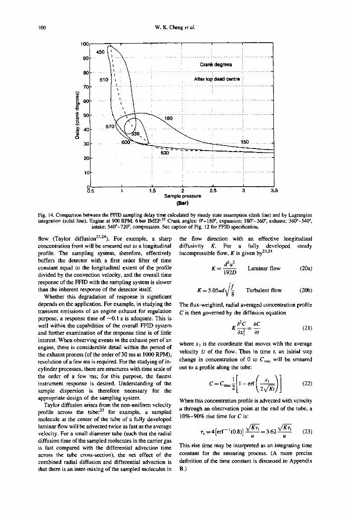
The behavior of the sampling system of Fig. 7 when used in in-cylinder sampling is shown in Fig. 13. In this figure, the horizontal axis is the crank angle at which the sample arrives and is detected by the detector. For example, at - 20°ATC, the total sampling delay time is
15 °. The FID signal at - 20°CA would thus read the HC concentration at the inlet at - 35°CA.
In Fig. 13, the total transit time which is expressed as the total delay crank angle in the figure, comprises three part: the Connecting Tube delay, the Settling Tube delay. and the Transfer Tube delay. The Connecting Tube delay is constant. In the early part of the compression process, the inlet pressure and thus the velocity are low; the delay is substantial. The major part of the delay is in the Settling Tube because the slow velocity there more than offset for the shorter length. The first 'kink' in the delay curve at - - 78 ° is caused by the laminar-to-turbulent flow transition. The second 'kink' at ~ - 70 ° is caused by the acoustic effect associated with the transition to choking in the Transfer Tube. Note that the delay in the Transfer Tube becomes approximately constant after it is choked.
It is preferable to operate the instrument in a window where the transit time is not excessive and approximately constant. This is because of the intermixing of sample
E 90
g,<
,'7"
8O
7O
60
5O
4O
3o
2O
10
0 -180
' /
(A) Transfer Tu~e Delay ~ Volume Flow Rate,,,~/
(C) Connecting 3~ Tube Delay t ,
-160 -140 -120 -100 -80 -60 -40 -20
Sample Arrival Crank Angle (deg. ATC)
8 ~
4 "6
2 ~ r r ,
Fig. 13. Behavior of the sampling system in Fig. 7 for in- cylinder sampling with engine running at 1000 RPM, 4.5 bar
~7 IMEP. The CP pressure was at 0.3 bar; the F1D pressure at 0.2 bar. The horizontal axis is the crank angle at which the sample arrives and is detected by the detector; 0 ° is defined as TDC compression. The plots terminate when the exit of the
Settling Tube is choked.
along the tube during the transit. If the transit time is long, the sample will be smeared out longitudinally and the time response of the instrument will be poor. With a time-varying transit time such as that which occurs during the early part of compression, the sample will be unevenly stacked in the sample line and it will be difficult to account for the extent of longitudinal mixing. This window depends on the engine operating condition and the sizing of the sampling system. The condition is more favorable at low rpm and high load so that the transit time is small. With a properly designed system. successful sampling could be done from prior to ignition through the power stroke, z2
The mass flow rate (traced back to the inlet) of the arrived sample is also shown in Fig. 13 (dotted line). At peak cylinder pressure, the flow is -270 /zg ms ~ (not shown in the figure). For comparison, the charge mass of a typical engine (of displacement of - 5 0 0 cm3/cylinder, and operating at the condition as described in the caption of Fig. 13) is - 6 0 0 mg. The period of high sample flow lasts only for a few milliseconds. Thus the sample flow would cause negligible perturbation of the combustion chamber condition.
The mass flow rate may be converted into a volume flow rate using the charge density at the time of entry of the sample (dash line in Fig. 13). For example, at ignition (at - 25°CA which, when a transit delay of --20 ° is added, corresponds to an arrival time of - 5°CA), the volume flow rate is - 6 m m 3 m s -~. If the overall integration time of the FFID is 2 ms, the sample volume would be - 1 2 m m 3. This volume would correspond to a hemisphere of --2 mm radius.
The comparison between the total transit time (the signal delay of the instrument) calculated by the steady state flow assumption Eq. (19) and by the Lagranian integration process is shown in Fig. 14 as a function of the cylinder pressure. With the steady flow assumption, the transit times are uniquely determined by the sample inlet pressure (i.e. the cylinder pressure) for a given FID configuration (dash line in Fig. 14). For unsteady flow, the transit time obtained by the Lagrangian integration is a function of the cylinder pressure history. The 'trajectory' of the transit times at different cylinder pressure levels from the expansion stroke to the compression stroke in a 4-stroke engine cycle is shown as the solid line in Fig. 14. The crank angle at the different parts of the cycle are marked on the trajectory. At high inlet pressure, there is not a big difference between the two calculations because of the earlier remark that the transit time is approximately constant after the flow in the Transfer Tube is choked. Thus the steady state transit time calculation is adequate for the high pressure part of the cycle. For the intake and the exhaust process, however, there are substantial differences between the two calculations.
3.5.2. Time constant
When a fluid sample flows through a small tube, there will be intermixing of the fluid in the direction of the
100 W.K. Cheng et al.
100
, .=)
90
80 ' 1
70
~¢ 6G ¢D
"O
"~ 50
40 a
30 . . . . . . . .
20
10
! Crank degrees
! i After top dead centre
I
1.5 2 2.5 3 3.5 Sample pressure
(Bar)
Fig. 14. Comparison between the FFID sampling delay time calculated by steady state assumption (dash line) and by Lagrangian 2 2 o o o o o integration (solid line), Engine at 900 RPM. 6 bar IMEP. Crank angles: 0 -180 °, expansion; i 80 -360, exhaust; 360 -540,
intake; 5400-720 °, compression. See caption of Fig. 12 for FFID specification.
flow (Taylor diffusion23'24). For example, a sharp concentration front will be smeared out to a longitudinal profile. The sampling system, therefore, effectively buffers the detector with a first order filter of time constant equal to the longitudinal extent of the profile divided by the convection velocity, and the overall time response of the FFID with the sampling system is slower than the inherent response of the detector itself.
Whether this degradation of response is significant depends on the application. For example, in studying the transient emissions of an engine exhaust for regulation purpose, a response time of -0.1 s is adequate. This is well within the capabilities of the overall FFID system and further examination of the response time is of little interest. When observing events in the exhaust port of an engine, there is considerable detail within the period of the exhaust process (of the order of 30 ms at 1000 RPM); resolution of a few ms is required. For the studying of in- cylinder processes, there are structures with time scale of the order of a few ms; for this purpose, the fastest instrument response is desired. Understanding of the sample dispersion is therefore necessary for the appropriate design of the sampling system.
Taylor diffusion arises from the non-uniform velocity profile across the tube: 23 for example, a sampled molecule at the center of the tube of a fully developed laminar flow will be advected twice as fast as the average velocity. For a small diameter tube (such that the radial diffusion time of the sampled molecules in the carder gas is fast compared with the differential advection time across the tube cross-section), the net effect of the combined radial diffusion and differential advection is that there is an inter-mixing of the sampled molecules in
the flow direction with an effective longitudinal diffusivity K. For a fully developed steady incompressible flow, K is given by 23"24
d2u 2 K = 192D Laminar flow (20a)
K = 5.05ud~/~ Turbulent flow (20b)
The flux-weighted, radial averaged concentration profile C is then governed by the diffusion equation
a2C 0C K 0x 2 = O~- (21)
where X l is the coordinate that moves with the average velocity U of the flow. Thus in time t, an initial step change in concentration of 0 to Cmax will be smeared out to a profile along the tube:
When this concentration profile is advected with velocity u through an observation point at the end of the tube, a 10%-90% rise time for C is:
rc = 4 [eft- '(0.8)] V ' ~ t = 3.62 V/-~t (23) U U
This rise time may be interpreted as an integrating time constant for the smearing process. (A more precise definition of the time constant is discussed in Appendix B.)
The fast-response flame ionization detector 101
The above incompressible flow results, however, could not be applied to the tubes of the FFID system where the velocity and density change substantially along the tube. The isothermal laminar compressible case was analyzed by S m i t h y For an isothermal laminar flow, the time constant rc is:
/P~+P~ (Laminar flow) (24a) 1.48 L
For hydrocarbon in air, the value of 1/Sc is in the range of 0.6-0.8; an average value of 0.7 may be taken. Hence, for laminar isothermal flow in a tube,
/p2+p2 (Laminar flow) (24b) L r e= 1 . 2 4 - ~ V ~-i~ - - p2
Note that the result is independent of the tube diameter. For turbulent isothermal flow, the above result is not
applicable because the radial velocity profile is different and because the concentration diffusion across the radius due to turbulence is different from the laminar case. A time constant, however, may be derived on an ad-hoc basis by noting that if Eq. (23) is written in a differential form as
~ x = (3.62) 2 . (25)
with K defined by Eq. (20), then the results of Eq. (24) follows. Assuming that i f the turbulent value of K (Eq.
(20)) is used, Eq. (25) also applies to a turbulent isother- mal flow; then*
L rc -- 1.44Re- 31,6 ~ ' ~ 1
P~ g R T V i
(Turbulent flow)
(26)
Because of the weak Re dependence, rc in Eq. (26) is not
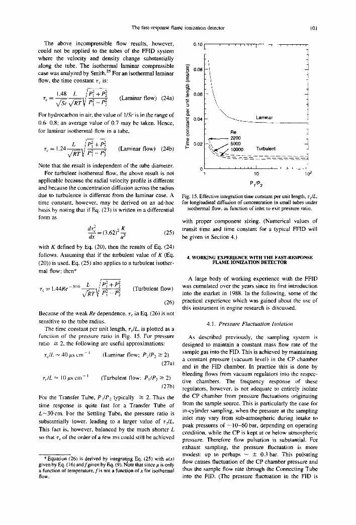
sensitive to the tube radius. The time constant per unit length, re~L, is plotted as a
function of the pressure ratio in Fig. 15. For pressure ratio --> 2, the following are useful approximations:
r~/L ~ 40 p.s cm - i (Laminar flow; Pt/P 2 >- 2)
(27a)
rc/L -~ 10 p.s c m - I (Turbulent flow; PI/P2 >- 2)
(27b)
For the Transfer Tube, PiP2 typically -> 2. Thus the
time response is quite fast for a Transfer Tube of
L--30 cm. For the Settling Tube, the pressure ratio is
substantially lower, leading to a larger value of rdL.
This fact is, however, balanced by the much shorter L
so that rc of the order of a few ms could still be achieved
* Equation (26) is derived by integrating Eq. (25) with u(x) given by Eq. (16) andfgiven by Eq. (9). Note that since t~ is only a function of temperature, f is not a function ofx for isothermal flow.
0.10
E" 0.08
g ¢-
_~ 0.06
e~
0.04
.E_ 0.02 I-
' ' ' 1 ' ' ' ' ' '
Re 2200
- - - 5000 loooo
- > . ~ - = _ _ . . . .
lO
P1/P 2
Laminar
Turbulent t . . . .
] I =
1 0 2
Fig. 15. Effective integration time constant per umt length, re~L, for longitudinal diffusion of concentration in small tubes under
isothermal flow, as function of inlet to exit pressure ratio.
with proper component sizing. (Numerical values of
transit time and time constant for a typical FFID will
be given in Section 4.)
4. WORKING EXPERIENCE WITH THE FAST-RESPONSE F L A M E I O N I Z A T I O N D E T E C T O R
A large body of working experience with the FFID was cumulated over the years since its first introduction into the market in 1988. In the following, some of the practical experience which was gained about the use of this instrument in engine research is discussed.
4.1. Pressure Fluctuation Isolation
As described previously, the sampling system is designed to maintain a constant mass flow rate of the sample gas into the FID. This is achieved by maintaining a constant pressure (vacuum level) in the CP chamber and in the FID chamber. In practice this is done by bleeding flows from vacuum regulators into the respec- tive chambers. The frequency response of these regulators, however, is not adequate to entirely isolate the CP chamber from pressure fluctuations originating from the sample source. This is particularly the case for in-cylinder sampling, when the pressure at the sampling inlet may vary from sub-atmospheric during intake to peak pressures of - 1 0 - 6 0 bar, depending on operating condition, while the CP is kept at or below atmospheric pressure. Therefore flow pulsation is substantial. For exhaust sampling, the pressure fluctuation is more modest: up to perhaps - --. 0.3 bar. This pulsating flow causes fluctuation of the CP chamber pressure and thus the sample flow rate through the Connecting Tube into the FID. (The pressure fluctuation in the FID is
102 W.K. Cheng et al.
usually negligible because the flow from the CP to the FID is small compared to the fuel and air flow rates, and to a first order of approximation, it does not change.)
In Section 3.4 it was shown what conditions need to be avoided, or what measures may be taken (in particular increasing the CP chamber volume) in order to reduce this effect to acceptable levels. It is worth adding here a few more details of the arguments involved. Typically the CP-FID pressure difference (APFIo) is --0.1 bar. A significantly higher value of APFID might:
I. lead to too high a flow into the FID chamber and disrupt the flame;
2. be unobtainable because of limitations on vacuum capacity;
3. lead to such a low FID chamber pressure that the flame is unstable or is unlightable.
A lower APFI D may be undesirable because: I. the'signal level may be too small; or 2. the percentage effect of any CP pressure variation
on the FID tube flow will be more serious. Thus if the FID sample flow (and hence signal)
variation is to be less than 1%, the variation of APFID should be less than 10 -3 bar.
For intake and exhaust measurements in which the flow pulsation is small, usually the effective CP chamber volume (actual volume plus the volume of the vacuum lines, typically - 1 0 0 cm 3) is sufficient to damp the CP pressure variation to acceptable level (see Section 3.4).
For in-cylinder measurements, several approaches are used to achieve an acceptable variation in CP pressure. The most obvious one is to increase the volume of the CP, which serves as a capacitor, and, together with the flow resistance of the Transfer Tube, acts as a first order filter. It was shown in Section 3.4 that for a typical
sampling arrangement with reasonable Transfer Tube working length (~300 mm) and diameter (0.2-0.5 mm), the necessary volume is ~ i ! for in-cylinder sampling applications. Usually an auxiliary ballast chamber is connected to the CP for this purpose. The connection may be conveniently done via tubing of reasonable diameter and length such that the flow resistance of the connection is much less than that of the Transfer Tube.
For sampling inlet pressures above atmospheric (for example, for in-cylinder sampling during the com- pression stroke), an effectively infinite CP chamber volume may be achieved easily by opening up the chamber to atmosphere. Operation in this mode is described in Ref. 26.
The other way to increase damping is to increase the flow resistance in the Transfer Tube. This method is less preferable because (a) it is difficult hardware-wise to use a tube diameter less than 0,2 mm, (b) small tubes tend to foul easily during operation, and (c) the frequency response of the sampling system suffers with a high flow resistance.
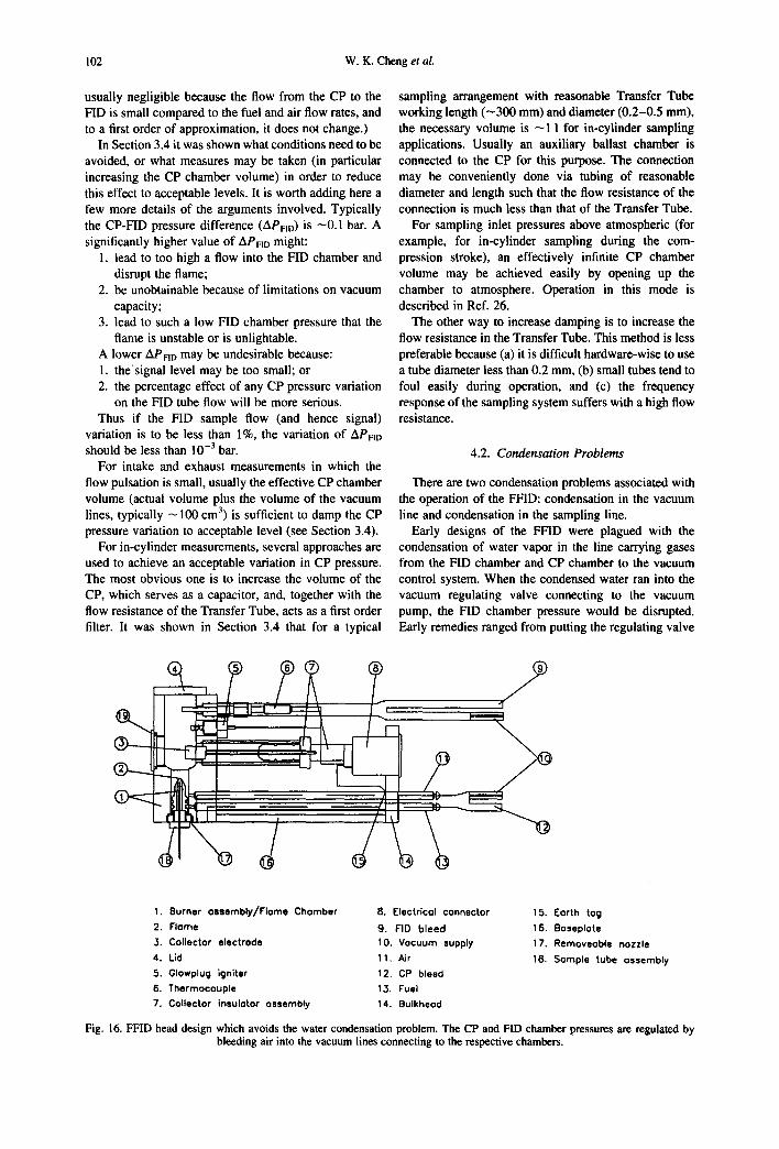
4.2. Condensat ion Problems
There are two condensation problems associated with the operation of the FFID: condensation in the vacuum line and condensation in the sampling line.
Early designs of the FFID were plagued with the condensation of water vapor in the line carrying gases from the FID chamber and CP chamber to the vacuum control system. When the condensed water ran into the vacuum regulating valve connecting to the vacuum pump, the FID chamber pressure would be disrupted. Early remedies ranged from putting the regulating valve
- . _ _ / , \ ,_ . ~ ~ - - L ~ ' .- , , / ' I
[ r
1. Burner assembly/Rome Chamber
2. Flame
3. Collector electrode 4. Lid
b. Glowplug igniter 6. Thermocouple 7. Collector ineulotor ossembly
8. Electrical connector
9. FID bleed 10. Vacuum supply 11. Air
12. CP bleed 1 ,,3. Fuel
14. Bulkhead
15. Earth tog
16. Boseplote 17. Removeoble nozzle 18. Sample tube assembly
Fig. 16. FFID head design which avoids the water condensation problem. The CP and F1D chamber pressures arc regulated by bleeding air into the vacuum lines connecting to the respective chambers.
The fast-response flame ionization detector 103
~ $ t e e l
Fig. 17. Heated sample line design to prevent liquid fuel condensation. Power is applied from the mid section of the sampling tube to ground (which is the engine chassis). Thus there are two branches oftbe electric current, respectively flowing towards the tip (at the
right side of the drawing) and towards the FFID connector (at the left side of the drawing).
close to the FFID and using heating tapes to keep both the vacuum line and the valve hot, to putting in a cold trap for the water in the vacuum line. This condensation problem was finally solved by a design shown in Fig. 16. Instead of regulating the FID pressure by a throttle valve before the vacuum pump, a valve regulating a bleed flow of ambient air to the vacuum line is used. In this way: (a) only air flows through the valve, and (b) the vacuum line receives the exhaust sample and FID chamber exhaust as well as a large quantity of ambient air, which raises the dew point of the gases in the vacuum line. Then, only when testing at sub-zero temperatures and at very high ambient humidity is trace heating of the vacuum lines necessary.
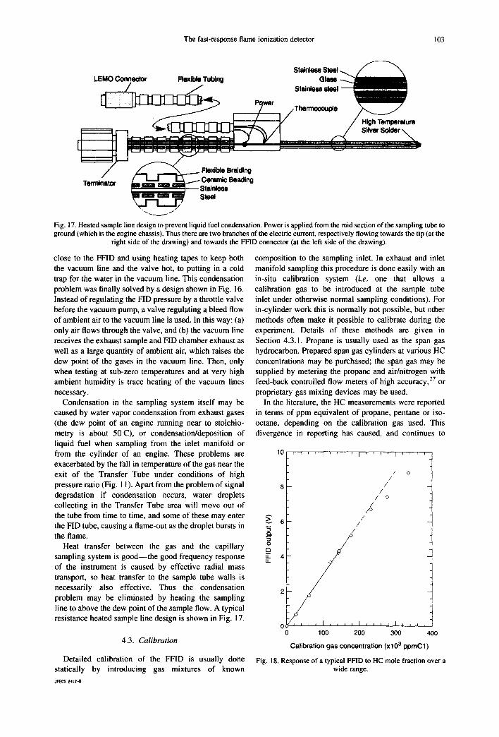
Condensation in the sampling system itself may be caused by water vapor condensation from exhaust gases (the dew point of an engine running near to stoichio- metry is about 50 C), or condensation/deposition of liquid fuel when sampling from the inlet manifold or from the cylinder of an engine. These problems are exacerbated by the fall in temperature of the gas near the exit of the Transfer Tube under conditions of high pressure ratio (Fig. i 1). Apart from the problem of signal degradation if condensation occurs, water droplets collecting in the Transfer Tube area will move out of the tube from time to time, and some of these may enter the FID tube, causing a flame-out as the droplet bursts in the flame.
Heat transfer between the gas and the capillary sampling system is good- - the good frequency response of the instrument is caused by effective radial mass transport, so heat transfer to the sample tube walls is necessarily also effective. Thus the condensation problem may be eliminated by heating the sampling line to above the dew point of the sample flow. A typical resistance heated sample line design is shown in Fig. ! 7.
4.3. Calibration
Detailed calibration of the FFID is usually done statically by introducing gas mixtures of known
JPECS 24:2-B
composition to the sampling inlet. In exhaust and inlet manifold sampling this procedure is done easily with an in-situ calibration system (i.e. one that allows a calibration gas to be introduced at the sample tube inlet under otherwise normal sampling conditions). For in-cylinder work this is normally not possible, but other methods often make it possible to calibrate during the experiment. Details of these methods are given in Section 4.3.1. Propane is usually used as the span gas hydrocarbon. Prepared span gas cylinders at various HC concentrations may be purchased; the span gas may be supplied by metering the propane and air/nitrogen with feed-back controlled flow meters of high accuracy, 27 or proprietary gas mixing devices may be used.
In the literature, the HC measurements were reported in terms of ppm equivalent of propane, pentane or iso- octane, depending on the calibration gas used. This divergence in reporting has caused, and continues to
10 ' ' ' ' I . . . . r ' ' ' ' I . . . .
/ 8 / /
/ o /
P /
--I
O a ,'r 4
2
0 , , , I . . . . I . . . . I i J l i
0 1 O0 2 0 0 3 0 0 4 0 0
Calibration gas c o n c e n t r a t i o n (x 1 0 3 p p m C 1 )
Fig. 18. Response of a typical FFID to HC mole fraction over a wide range.
104 W.K. Cheng et al.
cause substantial confusion. Since the FID is essentially a 'carbon counting' device (see Section 2.1), it would be reasonable to report the results in terms of ppmCl equivalent. Another misnomer is to refer to the ppm value as a concentration. Strictly speaking it is a mole fraction. It seems unlikely, however, that these unfortu- nate usages will change in the near future.
In an internal combustion engine, the values of the HC mole fraction (X~c) vary over a very broad dynamic range. The unburned gas may be rich, with a Xac of the order of 160000 ppmC1. The burned gas, on the other hand, may have XHC--100 ppmCl. A properly operating
FFID should be linear over the whole range. For very high values of XHC, however, the behavior may deviate from linear because the HC from the sample flow may affect the flame. This effect is illustrated in Fig. 18 for a typical FFID. Note that the region of non-linearity is for XHc > 2 × l05 ppmCl which is substantially above that of a stoichiometric mixture (--1.3 × l0 s ppmCl).
To calibrate the instrument against drift during an experiment, an in-situ procedure is often used. Usually a single point in-situ calibration is performed several times during the course of an experiment to tie down the complete calibration curve which is obtained off-line.
Sampling probe with build-in calibration
Span, Zero or Purge Air ~ ~ l / V a c u u m
to FID
Measure Mode Calibration and Purge Mode
Fig. 19. In-situ calibration arrangement for exhaust gas FFID measurements.
Sample Flow to FID
V A C U U M
' W A T E R ' ~ _ _ ~ - - - - - ] P = 0 . 9 5 FID
D.-~ 1 CALIBRATION B ~ L I G A S F L O W
I SAMPLE
A T M O S P H E R E
LENGTH DIA. TRANSIT [mini [mm] ~ [im~]
I (A)TRANSFER TUBE 100 0.3 1
(B) RESTRICTION 20 0.15 0.1
(C) EXPANSION TUBE 20 1.0 0.3
(D) CONNECTING TUBE 30 0.3 1.5
TOTAL 19
(E) BALLAST CHAMBER V~5 CC
Fig. 20. In-situ calibration arrangement for in-cylinder FFID measurements. 26
The fast-response flame ionization detector 105
4.3.1. Calibration techniques
For exhaust flow measurements, an in-situ calibration arrangement is shown in Fig. 19. The sampling inlet is surrounded by a jacket which is connected by a solenoid valve to the calibration gas. During normal operation, the FFID samples the exhaust gas. When calibration is needed, the solenoid valve is activated to send a jet of span gas to the exhaust. Then the FFID samples the span gas within the jet core which is not mixed with the exhaust gas. The amount of span gas introduced in the calibration process is small compared to the exhaust flow; thus in-situ calibration may be done without interrupting the engine operation.
The same procedure may be used for intake flow measurements. An additional benefit is that for measure- ments in port-fuel-injection engine, the same device could be used to provide a shroud of purge air around the sampling inlet during fuel injection so that ingestion of liquid droplets into the sampling line could be minimized.
The set-up for in-situ calibration of in-cylinder FFID measurements in every engine cycle is shown in Fig. 20. 26 Referring to the figure, the calibration method involves the passage of a span gas of a known HC mole fraction into the constant pressure (CP) chamber (E) of the detector. The CP chamber is kept at
atmospheric pressure in the experiment by venting it to the ambient. Whenever the sample flow rate is insufficient to displace the span gas at the inlet of the Connecting Tube (D), the pressure difference between the CP chamber and the FID chamber drives the span gas into the FID. For a naturally aspirated engine, this happens during the intake stroke when the cylinder pressure is sub-atmospheric. The signal in this period thus provides an in-situ calibration level for the HC measurement in the cycle.
Figure 2126 shows the typical FFID signal obtained in a firing engine with the sampling system shown in Fig. 20. The cylinder pressure trace is also shown. Because of the finite transit time from the sample line inlet to the detector, the actual FID signal has a phase lag with respect to the pressure trace. This transit time is a function of the cylinder pressure and the configuration of the sampling system. The FID signal in Fig. 21 was adjusted for this lag time. Starting from the LHS of this figure (at 0°CA), the FID sees only the span gas, which serves as a calibration for the HC measurement of the cycle. The detector signal drops during the initial stage of compression because the burned gas from the previous cycle which remains in the sample line is displaced into the detector as the line is purged by the fresh content of the cylinder. The blip in the signal at -100°CA is the result of the acoustic effect associated with the sonic
M
B
0
. . . . I . . . . I . . . . I ' F I I D ~ ] . ~ v d
• I~-C~md~r HC L ~ d
/ N \ x .
- ~ - , - - ~ - - r ~ ' ~ , , ~ , , ,
, 50
40
0 ' rO 0 100 200 300
k
2o | ¢.
I0
Degrees Crankaagle
Fig. 21. FFID signal from in-cylinder sampling with setup as shown in Fig. 20.
Table 3. Typical FFID characteristics for in-cylinder sampling
Pressure settings: Inlet = 5 bar CP = 0.547 bar FID = 0.480 bar Total transit time 3.7 ms Cumulative time constant 1.13 ms
Transfer Tube Settling Tube Connecting Tube
Tube diameter (mm) 0.51 1.52 0.30 Length (mm) 350 23 20 Temperature (°C) 150 150 150 Mass flow (mg s -I) 62.4 62.4 1.24 Reynolds No. 6582 2193 218 Transit time (ms) 2.94 0.31 0.50 Component time constant (ms) 0.17 1.08 0.28
106 W.K. Cheng et al.
transition at the exit of the Transfer Tube. Then the signal rises as fresh mixture of the current cycle is transported to the FID and the leveling out of the signal indicates that this purging process is completed.
4.4. Typical FFID Setting
The typical FFID operating characteristics are shown in Tables 3 -5 for in-cylinder, intake, and exhaust measurements. The FFID component dimensions are representative of common usage. The results are calculated based on steady isothermal flow through the sampling system. As discussed in Section 3, the calculations are adequate for assessing the performance of the sampling system.
The quantities of interest in these tables are the transit times, the cumulative time constants (which are the results of the Taylor longitudinal diffusion in the sampling system), and the mass flows. For each component (Transfer Tube, expansion tube and Con- necting Tube) the time constants are calculated by Eq. (24). Using the analogy between diffusion and the random walk problem, the cumulative time constant is the square root of the sum-of-squares of the component time constants.
The transit times are used to correct for the time delay of the instrument response. The time constant is a measure of the effective time resolution of the sampling system. Note that for in-cylinder sampling, the mass flow is quite substantial, and a correspondingly large pumping capacity is needed. Often a smaller diameter Transfer Tube (0.2 instead of 0.5 mm diameter) is used to lower the pumping requirement. For intake flow sampling,
there is a large transit time and time constant because of the small pressure differential across the Transfer Tube.
4.5. FFID Signal compensation
If the frequency response of the FFID system is known, a digital filter may be constructed to process the signal to compensate for the response time. An estimate of the frequency response may be obtained by assuming the instrument to be a first order system with a time constant given by the Taylor diffusion effect in the quasi- steady calculation. For in-cylinder sampling, the time constant, and thus the elements of the digital filter changes as a function of the cylinder pressure. For exhaust and intake measurements, this time constant is unchanged and a fixed filter could be used. A typical signal reconstruction is shown in Fig. 22. 28 Compared with the uncompensated signal (Fig. 22(a)), the recon- structed signal (Fig. 22(b)) shows much more detailed features: for example, the HC peak at EVO (at time -0 .012 s in the figure), which corresponds to the HC caused by valve leakage effect, is much more detectable in the reconstructed signal.
4.6. In-cylinder Sampling at Higher Engine Speeds
It is often desired to use the FFID to measure the in- cylinder unburned mixture equivalence ratio to assess the engine behavior. At high speed, because of the finite time response of the FFID (especially during the low cylinder pressure part of the cycle), the signal may not rise to the level representative of the unburned mixture. This fact is illustrated in Fig. 23. The data in this figure
Table 4. Typical FFID characteristics for intake sampling
Pressure settings Inlet = 0,5 bar CP = 0.3 bar FID = 0.25 bar Total transit time 27 ms Cumulative time constant 6.22 ms
Transfer Tube Settling Tube Connecting Tube
Tube diameter (mm) 0.51 1.52 0.30 Length (mm) 350 23 20 Temperature (°C) 150 150 150 Mass flow (mg s -I) 1.3 1.3 0.50 Reynolds No. 136 46 88 Transit time (ms) 18.5 7.9 0.66 Component time constant (ms) 2.89 5.50 0.32
Table 5. Typical FFID characteristics for exhaust sampling
Pressure settings: Inlet = 1.1 bar CP = 0.547 bar FID = 0.480 bar Total transit time 9.9 ms Cumulative time constant 3.9 ms
Transfer Tube Settling Tube Connecting Tube
Tube diameter (mm) 0.51 1.52 0.30 Length (mm) 350 23 20 Temperature (°C) 150 150 150 Mass flow (mg s i) 7.2 7.2 1.24 Reynolds No. 763 255 220 Transit time (ms) 6.83 2.61 0.50 Component time constant (ms) 2.20 3.18 0.28
The fast-response flame ionization detector 107
0.25
g ,
0.2
i0 .15 o
0.1 0
! , i
Ca) i
i J I 0.01 0.02 0.03 0.04 0.05 0.06
0.25 ! , ,
g i (b)
0.2 2
~0.15 0 ..r-
I I I I I
0"10 0.01 0.02 0.03 0.04 0.05 0.06 Time (s)
Fig. 22. Frequency response compensation for exhaust FFID measurement; engine at 2000 rpm under part load, sampling point very close to the exhaust valve; 2s (a) uncompensated signal; (b) signal compensated for by digital filtering.
were obtained from an engine operating at 1500 rpm and intake pressure of 0.4 bar. The sample inlet was at the ground electrode of the spark plug. Note that for the normal burning cycles (Trace (a)), the signal at flame arrival did not reach a plateau value that was indicative of the 'true' unburned mixture HC mole fraction (see Fig. 21 for comparison). A plateau was reached for a slow-burn cycle (Trace (b)) for which the flame arrived at a later time in the cycle. To obtai6 the proper signal, a technique of skip-firing one out of every 10 cycles were used: 29 only the 'flat' part of the FFID signal of the skip-fired cycle (Trace (c)) was used to determine the in-cylinder HC level.
ts00 n ~ 0 . ~ 21 °
M O ' I ' O I ~ G T I O t O [
e.e~ t
O.Ot
MINE CA Ccloa.) Fig. 23. Typical L~-'ID signal at low load and high spe l l (Pin~ke = 0.4 bar, 1500 rpm): Ca) traces of 4 normal cycles; (b) trace of a slow-burn cycle; (c) trace of skip firing cycle. 29 (Dip in trace (c) at --140*CA was an artifact because the CP chamber pressure
was not set low enough.)
The previous situation is most severe at high engine speed and low load, for which the transit time is long and thus the dispersion in the sampling system is significant, and for when the sample is taken from the vicinity of the spark plug because then the flame arrives quickly at the sample inlet. The situation could be improved by sampling at a position far from the spark plug so that flame arrival is delayed as much as possible, 3° or by shortening the sample line length to reduce the sampling system time constant. (Note that the time constant is almost independent of the tube diameters; see Eqs (24a,b) and (26).) Usually measurement is difficult for an engine speed higher than ~2000 rpm. If a measurement is only to be taken at steady state engine operating condition, the skip-firing technique is the most robust method and it could be used at significantly higher rpm.
There are many cases in which sampling at the vicinity of the spark plug is essential and the skip-firing technique cannot be used, for example, in the assessment of the A/F at ignition during an engine transient. This situation is evaluated by Crawford and Wallace 31. The peak of the signal (which does not show a plateau part) obtained from sampling from the vicinity of the spark plug is compared to the 'plateau' value of the signal obtained in the same cycle from sampling at a location at the maximum distance from the spark. The latter value is taken as the 'true' HC mole fraction of the unburned charge. The ratio of the two values (which is defined as the peak agreement in the paper) is shown in Fig. 24 as a function of engine speed. The engine was a CFR engine with a low compression ratio of 7.74 and was operating close to idle condition; thus the test condition was deliberately set to be adverse. Over the speed range of 900-1650rpm, the average of the ratios is ~97%
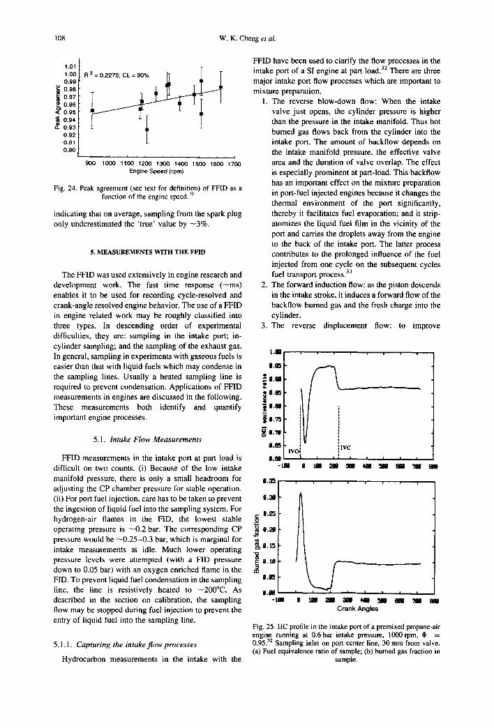
108 W.K. Cheng et al.
1.01 t .00 0.99
e~0.98 0.97 0.96 0.95
"~ 0.94 ~. 0,93
0.92 0.91 0.90
R2=0'2275;CL=90% ~ ~ I I
900 1000 1100 1200 1300 1400 1500 1600 1700 Engine Speed (rpm)
Fig. 24. Peak agreement (see text for definition) of FFID as a function of the engine speed. 31
indicating that on average, sampling from the spark plug only underestimated the 'true' value by - 3 % .
5. MEASUREMENTS WITH THE FFID
The FFID was used extensively in engine research and development work. The fast time response ( - m s ) enables it to be used for recording cycle-resolved and crank-angle resolved engine behavior. The use of a FFID in engine related work may be roughly classified into three types. In descending order of experimental difficulties, they are: sampling in the intake port; in- cylinder sampling; and the sampling of the exhaust gas. In general, sampling in experiments with gaseous fuels is easier than that with liquid fuels which may condense in the sampling lines. Usually a heated sampling line is required to prevent condensation. Applications of FFID measurements in engines are discussed in the following. These measurements both identify and quantify important engine processes.
5.1. Intake Flow Measurements
FFID measurements in the intake port at part load is difficult on two counts. (i) Because of the low intake manifold pressure, there is only a small headroom for e.a~ adjusting the CP chamber pressure for stable operation. (ii) For port fuel injection, care has to be taken to prevent 0.a0 the ingestion of liquid fuel into the sampling system. For il.25 hydrogen-air flames in the FID, the lowest stable .~ operating pressure is ~0.2 bar. The corresponding CP ~ 0 .~ pressure would be -0 .25 -0 .3 bar, which is marginal for intake measurements at idle. Much lower operating ~ e.t5
" U
pressure levels were attempted (with a FID pressure =~ 0.t0 down to 0.05 bar) with an oxygen enriched flame in the t~ FID. To prevent liquid fuel condensation in the sampling 0 .~ line, the line is resistively heated to --200°C. As described in the section on calibration, the sampling flow may be stopped during fuel injection to prevent the entry of liquid fuel into the sampling line.
5.1.1. Capturing the intake flow processes
Hydrocarbon measurements in the intake with the
FFID have been used to clarify the flow processes in the intake port of a SI engine at part load. 32 There are three major intake port flow processes which are important to mixture preparation.
1. The reverse blow-down flow: When the intake valve just opens, the cylinder pressure is higher than the pressure in the intake manifold. Thus hot burned gas flows back from the cylinder into the intake port. The amount of backflow depends on the intake manifold pressure, the effective valve area and the duration of valve overlap. The effect is especially prominent at part-load. This backflow has an important effect on the mixture preparation in port-fuel injected engines because it changes the thermal environment of the port significantly, thereby it facilitates fuel evaporation; and it strip- atomizes the liquid fuel film in the vicinity of the port and carries the droplets away from the engine to the back of the intake port. The latter process contributes to the prolonged influence of the fuel injected from one cycle on the subsequent cycles fuel transport process. 33
2. The forward induction flow: as the piston descends in the intake stroke, it induces a forward flow of the backflow burned gas and the fresh charge into the cylinder.
3. The reverse displacement flow: to improve
t.lO
| . ~
o
~. | . M ~ | . ~
~. 11.711
| . ~ O.W IvGI
-Ira O
O . J I I I
Crank Angles
i ivc i
i i t i t t i
Fig. 25. HC profile in the intake port of a premixed propane-air engine running at 0.6bar intake pressure, 1000rpm, ~ = 0.95. 32 Sampling inlet on port center line, 30 mm from valve. (a) Fuel equivalence ratio of sample; (b) burned gas fraction in
sample.
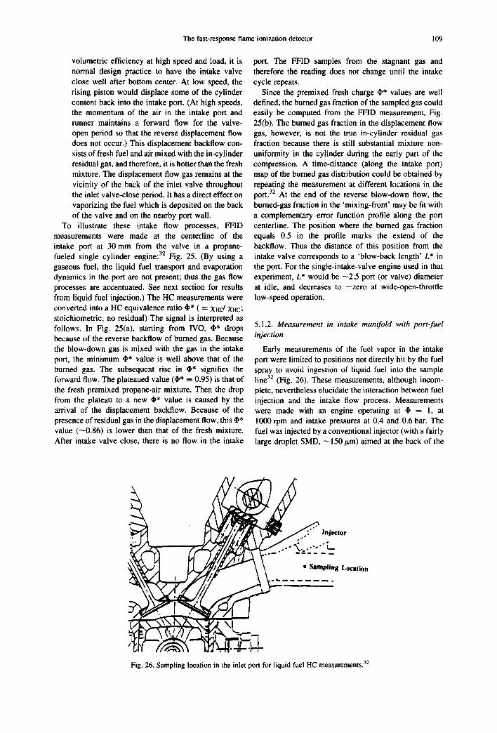
The fast-response flame ionization detector 109
volumetric efficiency at high speed and load, it is normal design practice to have the intake valve close well after bottom center. At low speed, the rising piston would displace some of the cylinder content back into the intake port. (At high speeds, the momentum of the air in the intake port and runner maintains a forward flow for the valve- open period so that the reverse displacement flow does not occur.) This displacement backflow con- sists of fresh fuel and air mixed with the in-cylinder residual gas, and therefore, it is hotter than the fresh mixture. The displacement flow gas remains at the vicinity of the back of the inlet valve throughout the inlet valve-close period. It has a direct effect on vaporizing the fuel which is deposited on the back of the valve and on the nearby port wall.
To illustrate these intake flow processes, FFID measurements were made at the centerline of the intake port at 30 mm from the valve in a propane- fueled single cylinder engine; 32 Fig. 25. (By using a gaseous fuel, the liquid fuel transport and evaporation dynamics in the port are not present; thus the gas flow processes are accentuated. See next section for results from liquid fuel injection.) The HC measurements were converted into a HC equivalence ratio #~* ( = xHc/Xsc; stoichiometric, no residual) The signal is interpreted as follows. In Fig. 25(a), starting from IVO, q~* drops because of the reverse backflow of burned gas. Because the blow-down gas is mixed with the gas in the intake port, the minimum cI,* value is well above that of the burned gas. The subsequent rise in q,* signifies the forward flow. The plateaued value (q~* = 0.95) is that of the fresh premixed propane-air mixture. Then the drop from the plateau to a new ~* value is caused by the arrival of the displacement backflow. Because of the presence of residual gas in the displacement flow, this q,* value (-0.86) is lower than that of the fresh mixture. After intake valve close, there is no flow in the intake
port. The FFID samples from the stagnant gas and therefore the reading does not change until the intake cycle repeats.
Since the premixed fresh charge ~* values are well defined, the burned gas fraction of the sampled gas could easily be computed from the FFID measurement, Fig. 25(b). The burned gas fraction in the displacement flow gas, however, is not the true in-cylinder residual gas fraction because there is still substantial mixture non- uniformity in the cylinder during the early part of the compression. A time-distance (along the intake port) map of the burned gas distribution could be obtained by repeating the measurement at different locations in the port. 32 At the end of the reverse blow-down flow, the burned-gas fraction in the 'mixing-front' may he fit with a complementary error function profile along the port centerline. The position where the burned gas fraction equals 0.5 in the profile marks the extend of the hackflow. Thus the distance of this position from the intake valve corresponds to a 'blow-back length' L* in the port. For the single-intake-valve engine used in that experiment, L* would be -2.5 port (or valve) diameter at idle, and decreases to -zero at wide-open-throttle low-speed operation.
5.1.2. Measurement in intake manifold with port-fuel injection
Early measurements of the fuel vapor in the intake port were limited to positions not directly hit by the fuel spray to avoid ingestion of liquid fuel into the sample line 32 (Fig. 26). These measurements, although incom- plete, nevertheless elucidate the interaction between fuel injection and the intake flow process. Measurements were made with an engine operating at q, = l, at 1000 rpm and intake pressures at 0.4 and 0.6 bar. The fuel was injected by a conventional injector (with a fairly large droplet SMD, - 150 ttm) aimed at the back of the
. " i
! •
I n j e c t o r
. .-" ..-.. _ _ ~
• S a m p l i n g L o c a t i o n
2 . . : - - - - - . . . .
Fig. 26. Sampling location in the inlet port for liquid fuel HC measurements. 32
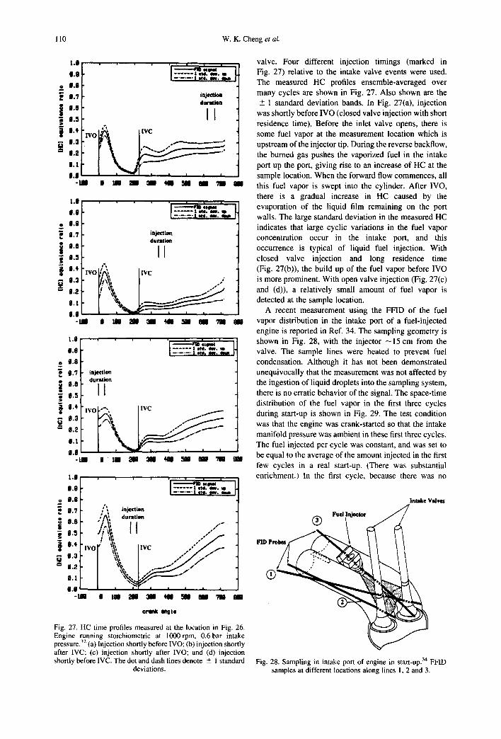
110 W.K. Cheng et al.
t.I ° I I
I ~ .wu l / I , I I . . . . . . I ~mJ. ~ . m I,
o 0 . 0 ~ 1 1.7 i inj~.tI~l
dwitlon I.el
i,.5 It
_-_J"' -opt,.., I w / ° ,
- , . , r \
I . I I I I -I I I I I | I I I I
L.I
I . I
o I . I !
I . ?
i I .O
! i , t
- - 1 . 3
- - 1 , 2
O.l l . I
o I
• I I I
. . . . . . 1 I l l . I .
injectlo~ durutlon
II l V ° t ~ ' I IvC ...
I
t . I , I I I
i . . . . . . I e t O . 4 1 t o MID 1.8 I . . . . . . t oTd. m*. o 6.8
0/7 injection duration
i ° " il i 0 . 5
! °'* , I 0.3 I
r "-:- - 0.I~ / j . 1
-I I I I I 41I I I ?II I
* . I
I .O
o 0.8
valve. Four different injection timings (marked in Fig. 27) relative to the intake valve events were used. The measured HC profiles ensemble-averaged over many cycles are shown in Fig. 27. Also shown are the --- 1 standard deviation bands. In Fig. 27(a), injection
was shortly before IVO (closed valve injection with short residence time). Before the inlet valve opens, there is some fuel vapor at the measurement location which is upstream of the injector tip. During the reverse backflow, the burned gas pushes the vaporized fuel in the intake port up the port, giving rise to an increase of HC at the sample location. When the forward flow commences, all this fuel vapor is swept into the cylinder. After IVO, there is a gradual increase in HC caused by the evaporation of the liquid film remaining on the port walls. The large standard deviation in the measured HC indicates that large cyclic variations in the fuel vapor concentration occur in the intake port, and this occurrence is typical of liquid fuel injection. With closed valve injection and long residence time (Fig. 27(b)), the build up of the fuel vapor before IVO is more prominent. With open valve injection (Fig. 27(c) and (d)), a relatively small amount of fuel vapor is detected at the sample location.
A recent measurement using the FFID of the fuel vapor distribution in the intake port of a fuel-injected engine is reported in Ref. 34. The sampling geometry is shown in Fig. 28, with the injector ~15 cm from the valve. The sample lines were heated to prevent fuel condensation. Although it has not been demonstrated unequivocally that the measurement was not affected by the ingestion of liquid droplets into the sampling system, there is no erratic behavior of the signal. The space-time distribution of the fuel vapor in the first three cycles during start-up is shown in Fig. 29. The test condition was that the engine was crank-started so that the intake manifold pressure was ambient in these first three cycles. The fuel injected per cycle was constant, and was set to be equal to the average of the amount injected in the first few cycles in a real start-up. (There was substantial enrichment.) In the first cycle, because there was no
Intake Valves
- " . . 4 , ~ Fuel Injector
II i 1 . 5 / / '
i IVO lVC o.~
/
| i | i i i I •
l J - I ° I I I I HO ! MB ' ; U I
Fig. 27. HC time profiles measured at the location in Fig. 26. Engine running stoichiometric at 1000rpm, 0.6bar intake pressure. 32 (a) Injection shortly before IVO; (b) injection shortly after IVC; (c) injection shortly after IVO; and (d) injection shortly before IVC. The dot and dash lines denote _+ I standard Fig. 28. Sampling in intake port of engine in start-up. 34 FFID
deviations, samples at different locations along lines I, 2 and 3.
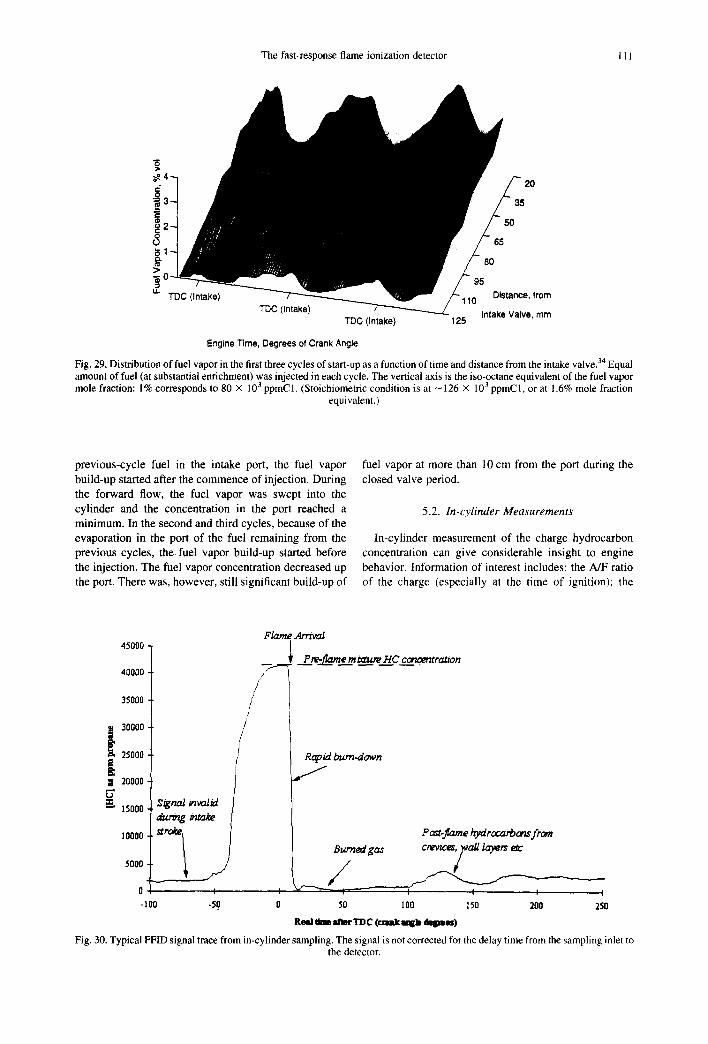
The fast-response flame ionization detector 111
TDC (Intake)
Engine Time, Degrees of Crank Angle
20
5
:e, from
, , , , ~ . ~ , v e , m m 125
Fig. 29. Distribution of fuel vapor in the first three cycles of start-up as a function of time and distance from the intake valve. 34 Equal amount of fuel (at substantial enrichment) was injected in each cycle. The vertical axis is the iso-octane equivalent of the fuel vapor mole fraction: 1% corresponds to 80 × 103 ppmC1. (Stoichiometric condition is at -126 × 103 ppmC1, or at 1.6% mole fraction
equivalent.)
previous-cycle fuel in the intake port, the fuel vapor build-up started after the commence of injection. During the forward flow, the fuel vapor was swept into the cylinder and the concentration in the port reached a minimum. In the second and third cycles, because of the evaporation in the port of the fuel remaining from the previous cycles, the fuel vapor build-up started before the injection. The fuel vapor concentration decreased up the port. There was, however, still significant build-up of
fuel vapor at more than 10 cm from the port during the closed valve period.
5.2. In-cylinder Measurements
In-cylinder measurement of the charge hydrocarbon concentration can give considerable insight to engine behavior. Information of interest includes: the A/F ratio of the charge (especially at the time of ignition); the
45000 -
4 0 0 0 0 -
35000 -
30000 -
25000
I 2oooo U'
m. ~5ooo Stgna2 mval/d
I0000 s~ro~e
5000
0
-lO0 -50
/ / /
/
/
Flame An~ol
~ . . _C~eCm ~ua~ HC cencentraUon
Rapid bum-down . f t
Bw'n~l ga¢
50
p ost-fl.ame hyarocaeoans frorn crevr.es/wa# layers
I I I I
100 150 200 250
g w l ttme afmr TDC (mink aagb da~. - )
Fig. 30. Typical FFID signal trace from in-cylinder sampling. The signal is not corrected for the delay time from the sampling inlet to the detector.
112 W.K. Cbeng et al.
variation of this ratio spatially within one cycle and temporally from cycle to cycle; the residual gas fraction of the charge. The post-flame HC signal signature can also be used to elucidate the in-cylinder storage and release HC mechanisms. 35
A typical FFID signal trace from in-cylinder sampling is shown in Fig. 30. The signal was not corrected for the delay time between the sample inlet and the detector. Starting from the left hand side of the trace, the signal is low because of the burned gas left over from the previous cycle. As fresh charge comes in and mixes with the residual gas, the signal rises gradually. Meaningful deduction, however, could not be made from this part of the signal because during this period the FFID response is slow (due to the low sample inlet pressure during the intake process). As the cylinder pressure rises in compression, the FFID response improves. At some point in the compression stroke, the signal reaches a plateau level which signifies the pre-flame HC mole fraction. This HC mole fraction is lower than that of the air/fuel mixture because of the presence of residual gas. Then there is an abrupt drop in the signal when the flame arrives. The fall-time could be interpreted as the response time of the FFID since the flame traverse time across the sample inlet is negligible ( --< 0.1 ms). The signal remains close to zero when the sample inlet is exposed to burned gas. In the later part of the cycle, however, the FFID detects post-flame hydrocarbons which are released from crevices and oil layer. The signature of the FFID signal here depends on the location of the sample inlet, and it could be used to confirm features of the in-cylinder HC mechanisms such as the out-gassing from crevices and the roll up of the HC layer on the liner into a vortex as the piston ascends.
5.2. I. In-cylinder measurement o f air~fuel ratio
One of the first uses to which the FFID was put was to measure charge inhomogeneity and cyclic variability. Using a propane fueled single cylinder research engine,
,
Air
FID w~age.
l t
Fig. 31, Various signals recorded during a fast throttle opening at 2000 RPM which increased engine torque from 5 to 98 Nm. ~9 Mixture strength just before transient is stoichiometric. Engine
management compensation strategy was disabled.
0 ~ 40 ~ N
= I . . . . ' . . . . ' ~ i ' . . . . " "
~ ° • I . "
2
o ~ 400 ~ 0
Cycle Number
) $ 10 15 20
~Z "~ l~ • "I
;I I' ' J ! I I I l ' " , ,J 7 0 , , , ~ ; l l t l l , l ' ; e l l . . . . I , , ; , I , , , , I , , , i 1 0
25 50 75 100 ~ 150
Cycle Number
Fig. 32. In-cylinder HC mole fraction and gross IMEP as a function of cycle number and time since start of injection. 26 Engine speed kept constant at 900 RPM; MAP = 0.5 bar; ¢ = 1.0 (based on the amount of fuel injected and the steady state air flow rate); spark timing fixed at 20°BTC; initial engine temperature ~20°C. Top: 720 cycles of data; bottom:
first 150 cycles of data in an expanded scale.
20 ' ' ' I ' ' ' ' i . . . . I . . . . / I ' '
0 First Firing Cycle / " 500/ ~. / /
¢ in i = 1 0 / / 4 0 °/~, " ~ . ° \ //-- 0
,-= x'//~//// ;0o~ ~ 3 0 0 / "
._o 10 " / f/ / - ,, \ I / /
CD / / ' ~ .~- ]. *~ 5 . i -
0 , - i , , I . . . . I . . . . I . . . . I i = 0 I0 20 30 40
Cycle Number
Fig. 33. 'Unaccounted-for' fuel accumulation (normalized by the amount of one injection): 35 900 RPM; MAP = 0.5 bar; spark timing @20°BTC; initial engine temperature ~20°C. The circle on each trace marks the first cycle of significant positive IMEP. The dash lines represent the amount if a fixed
percentage of the injected fuel was not 'accounted-for'.
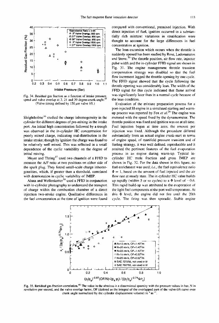
The fast-response flame ionization detector 113
40
35
c 30 .9
25: LL o~ 20
"~ 15
"N 10 I I
5 i
o 0.2
o 0
Equivalence Ratio = 0.95 3 o Valve Overlap; 900 rpm
A 2 1 ° Valve Ovedap; 900 rpm O 3 9 ° Valve Ovedap; 900 rpm O 30 Valve Ovedap;1500 rpm
0 x 21 ° Valve Overlap;1500 rpm
O A t~
<>
n
0.3 0.4 0.5 0.6 0.7 0.8 0.9 1.0 1.1
Intake Pressure (Bar)
Fig. 34. Residual gas fraction as a function of intake pressure, speed and valve overlap at 3, 21 and 39 degree-crank-angle. 29
(Valve timing defined by 150/zm valve lift.)
Sleightholme 36 studied the charge inhomogeneity in the cylinder for different degrees of pre-mixing in the intake port. An initial high concentration followed by a trough was observed in the in-cylinder HC concentration for poorly mixed charge, indicating mal-distribution in the intake stroke; though by ignition the charge was found to be relatively well mixed. This was reflected in a small dependence of the cyclic variability on the degree of initial mixing.
Meyer and Thring 37 used two channels of a FFID to measure the A/F ratio at two positions on either side of the spark plug. They found small-scale charge inhomo- geneities, which, if greater than a threshold, correlated with deterioration in cyclic variability of IMEP.
Abata and Wellenkotter 3s used a FFID in conjunction with in-cylinder photography to understand the transport of charge within the combustion chamber of a direct injection two-stroke engine. Qualitative differences in the fuel concentration at the time of ignition were found
compared with conventional, premixed injection. With direct injection of fuel, ignition occurred in a substan- tially rich mixture: variations in stratification were thought to account for the large differences in fuel concentration at ignition.
The lean excursion which occurs when the throttle is suddenly opened has been studied by Rose, Ladommatos and Stone. 39 The throttle position, air flow rate, injector pulse width and the in-cylinder FFID signal are shown in Fig. 31. The engine management throttle transient compensation strategy was disabled so that the fuel flow increment lagged the throttle opening by one cycle. The FFID signal showed that the cycle following the throttle opening was considerably lean. The width of the FFID signal for this cycle indicated that flame arrival was significantly later than in a normal cycle because of the lean condition.
Evaluation of the mixture preparation process for a port-injected SI engine in a simulated starting and warm- up process was reported by Fox et al. 26 The engine was motored with the speed fixed by the dynamometer. The throttle position was fixed and ignition was on at all time. Fuel injection began at time zero; the amount per injection was fixed. Although the procedure differed substantially from an actual engine crank-start in terms of engine speed, of manifold pressure transient and of fueling strategy, it was well defined, reproducible and it retained the pertinent features of the fuel evaporation process in an engine during warm-up. Typical in- cylinder HC mole fraction and gross IMEP are shown in Fig. 32. For the data shown in this figure, no fuel enrichment was used; i.e., the fuel equivalence ratio ¢I, = 1, based on the amount of fuel injected and the air flow rate at steady state. The in-cylinder HC value builds up rapidly (within 5 or so cycles) to a • level of -0 .6 . This rapid build-up was attributed to the evaporation of the light fuel components at the port wall temperature. At this (I) level, the engine did not fire until the 20th cycle. The firing was then sporadic. Stable engine
1.5
9" 1.0 e~ -I x~ 0.5
o o
' ' ' ' I ' ' ' ' I ' ' ' ' I . . . . I " / ~
J
o , ~ : ~ '@ @ @
~ : @ m ° ~ @ A N = 1 5 r e v / s , OF=1.43°/m
, ~k @ @ • N=20 rev/s, OF=1.43°/m • N=25 rev/s, OF=1.43e/m /~ N=15 rev/s, OF=0.52°/m o N=25 rev/s, OF=0.52°/m
SAE 720256, not used in fit @ SAE 760765, not used in fit
i i i I I i i , , i i , I i I I I I I I i I
0.2 0.4 0.6 0.8
(pi/Pe)°87(OF/N),J(pe-Pi) / [(pi/pe)°74(:l)/rc ]
4O Fig. 35. Residual gas fraction correlation. The value in the abscissa is a dimensional quantity with the pressure values in bar, N in revolution per second, and the valve overlap factor, OF (defined as the integral of the overlapped part of the valve-lift curve over
crank angle normalized by the cylinder displacement volume) in ° m-L
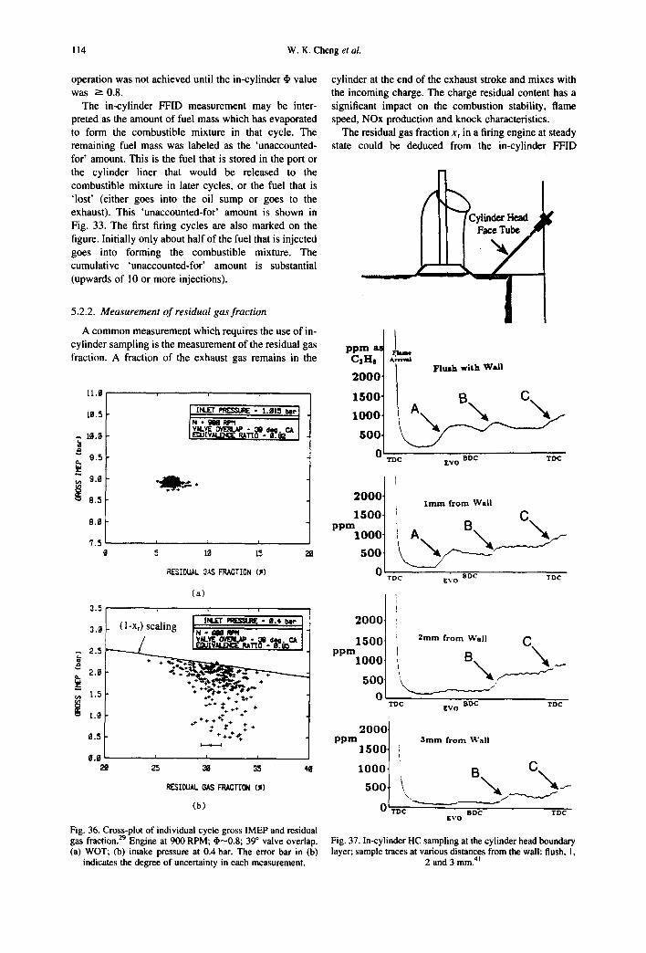
114 W.K. Cheng et al.
operation was not achieved until the in-cylinder 4, value was --> 0.8.
The in-cylinder FFID measurement may be inter- preted as the amount of fuel mass which has evaporated to form the combustible mixture in that cycle. The remaining fuel mass was labeled as the 'unaccounted- for' amount. This is the fuel that is stored in the port or the cylinder liner that would be released to the combustible mixture in later cycles, or the fuel that is ' lost ' (either goes into the oil sump or goes to the exhaust). This 'unaccounted-for ' amount is shown in Fig. 33. The first firing cycles are also marked on the figure. Initially only about half of the fuel that is injected goes into forming the combustible mixture. The cumulative 'unaccounted-for' amount is substantial (upwards of 10 or more injections).
5.2.2. Measurement of residual gas fraction
A common measurement which requires the use of in- cylinder sampling is the measurement of the residual gas fraction. A fraction of the exhaust gas remains in the
l l .~
tg.5
-- i@.~
~ 9.5
~ 9A!
~ 8.5
7.5
J INI.ET v~,~'~-~E • I.~15 0er 1 N - 9U V~ I VAI.VE - 09 d q CA
r i
5 IQ5 15 2~
~SIDUAL 3AS FRACTION (~)
3.5
3.ff
2.5
2.8
t.5
t.8
8.5
oa
(a)
J-Xrl scanng IN we ~ ] "J
°% * ** t+ "
+ +
I I f
25 3g 35
RESIDUAL GAS FRACTION (~)
(b)
Fig. 36. Cross-plot of individual cycle gross IMEP and residual 29 gas fraction. Engine at 900 RPM; ¢~0.8; 39 ° valve overlap.
(a) WOT; (b) intake pressure at 0.4 bar. The error bar in (b) indicates the degree of uncertainty in each measurement.
cylinder at the end of the exhaust stroke and mixes with the incoming charge. The charge residual content has a significant impact on the combustion stability, flame speed, NOx production and knock characteristics.
The residual gas fraction Xr in a firing engine at steady state could be deduced from the in-cylinder FFID
T
-I p p m al
C : H s
2 0 0 0
1 5 0 0 '
1 0 0 0
5 0 0
0
Am,~ l
Flush with Wall
B D C T D C T D C E V O
2 0 0 0
1 5 0 0
p p m l o 0 0
5 0 0
0
2 0 0 0
1 5 0 0 p p m
1000.
500 0
Imm f rom Wall
I A. B \ C'x,,,a ~_
TDC EDC TDC E V O
2ram from Wall C
T D C B O C T D C g V O
2ooo4 I p p m / i 3ram from Wall
C lOOO] oo ' B,,,,, 0 TDC • B D C ' T D C
E V O
Fig. 37. In-cylinder HC sampling at the cylinder head boundary layer; sample traces at various distances from the wall: flush, I,
2 and 3 ram. 'tn
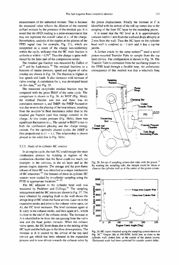
The fast-response flame ionization detector 115
measurement of the unburned mixture. This is because the measured value reflects the dilution of the metered air/fuel mixture by the presence of the residual gas. It is noted that the FFID reading is a point-measurement that may not represent the overall value of Xr of the charge. Nevertheless, analysis of the ripples at the plateau of the FFID signal (see for example, Fig. 21), which are interpreted as a result of the charge non-uniformity within the cycle, indicates that the HC mole fraction is uniform to within - 12% 9. Thus the charge is quite well- mixed by the later part of the compression stroke.
The residual gas fraction was measured by Galliot et al. 29 and by Ladomatos. 3° The residual fractions as a function of intake pressure, speed and degree of valve overlap are shown in Fig. 34. The fraction is highest at low speeds and loads. It also increases with increase of valve overlap. A correlation for Xr was developed based on this data, 4° see Fig. 35.
The measured in-cylinder residual fraction may be compared with the gross IMEP of the same cycle. The comparison is shown in Fig. 36. At WOT (Fig. 36(a)), the residual fraction was low and there was no correlation between Xr and IMEP: the IMEP fluctuation was due more to the phasing of the heat release, resulting from the in-cylin~'er fluid mechanics rather than to the residual gas fraction (and thus energy content) in the charge. At low intake pressure (Fig. 36(b)), there was significant fluctuation in xr. The spread in IMEP is due to both the combustion phasing and the charge energy content. For the optimally phased cycles, the IMEP is thus proportional to (1 - x0. This relationship is shown plotted as the solid line in Fig. 36(b).
5.2.3. Study o f in-o'linder HC sources
In an engine cycle, the fuel HC could escape the main combustion process by residing in regions of the combustion chamber that the flame could not reach; for example: in the crevices, in the oil layer and in the porous engine deposits. The storage and the post-flame release of these HC was identified as a major mechanism of HC emissions. 35 The features of these in-cylinder HC sources were studied by in-cylinder sampling using the FFID at appropriate locations. 4~-43
The HC adjacent to the cylinder head wall was measured by Peckham and Collings. 4j The sampling arrangement and the HC traces are shown in Fig. 37. The trace obtained by sampling flush to the wall shows the abrupt drop of HC when the flame arrives. Later on in the expansion stroke and prior to the exhaust valve open, (at A), the HC level increases. The level increases again at B, early in the exhaust stroke, and then again at C, which is close to the end of the exhaust stroke. The increase at A is identified to be from the out-gassing from the valve seat and the head gasket crevices. When the exhaust valve opens, the HC level drops due to the mixing of the HC layer and the bulk gas in the blow-down process. The increase at B is caused by the arrival of the top land crevice gas which has been released in the expansion process and is now driven towards the exhaust valve by
the piston displacement. Finally the increase at C is identified with the arrival of the roll-up vortex due to the scraping of the liner HC layer by the ascending piston.
It is noted that the HC level at A is approximately constant within 1 mm from the wall and drops abruptly at 2 mm from the wall. Thus the HC layer on the cylinder head wall is confined to --1 mm and it has a top-hat profile.
A further article by the same authors 43 used a novel piston-mounted Transfer Tube to sample from the top land crevice. The configuration is shown in Fig. 38. The Transfer Tube is connected from the oscillating piston to the FFID head through a flexible loop. An unfortunate consequence of this method was that a relatively long
S,mpti~S
- - - -v \ F \ \ I [ 1 . / ~D r
Fig. 38. Set-up of sampling system that rides with the piston. 43 By rotating the sampling tube, the sample could be taken at close to the cylinder wall or at the center of the piston crown.
8oo0
7 0 0 0 !
~ 6000
~5ooo ,ooo
1ooo
i l - - O~mm from C'/li~ller W ~
i A ........... 2 ~ from Cyl~der WaU
~'~
!! c
0 5 0 1 (30 150 200 250
~ s i ~ Croak A~S~ t ~ g ]
Fig. 39.43HC traces, obtained, using the sampling system shown m Fig. 38. " Engine tdle at 500 RPM. Solid line: at close to the cylinder wall; dotted line: at the center of the piston crown. Horizontal scale had been corrected for sample system delay.
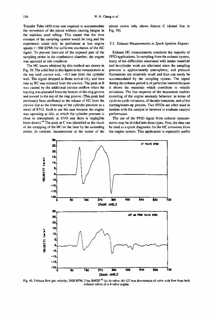
116 W.K. Cheng et al.
Transfer Tube (450 mm) was required to accommodate the movement of the piston without causing fatigue in the stainless steel tubing. This meant that the time constant of the sampling system would be long and the experiment could only be performed at low engine speeds (~500 RPM) for sufficient resolution of the HC signal. To prevent burn-out of the exposed part of the sampling probe in the combustion chamber, the engine was operated at idle condition.
The HC traces obtained by this method are shown in Fig. 39. The solid line in this figure is the measurement at the top land crevice exit, --0.5 mm from the cylinder wall. The signal dropped at flame arrival (A); and then rose as HC was released from the crevice. The peak at B was caused by the additional crevice outflow when the top ring was unseated from the bottom of the ring groove and moved to the top of the ring groove. (This peak had previously been attributed to the release of HC from the crevice due to the lowering of the cylinder pressure as a result of EVO. Such is not the case because the engine was operating at idle, at which the cylinder pressure is close to atmospheric at EVO and there is negligible blow-down). 44 The peak at C was identified as the result of the scrapping of the HC on the liner by the ascending piston. In contrast, measurement at the center of the
piston crown only shows feature C (dotted line in Fig. 39).
5.3. Exhaust Measurements in Spark Ignition Engines
Exhaust HC measurements constitute the majority of FFID applications. In sampling from the exhaust system, many of the difficulties associated with intake manifold and in-cylinder work are alleviated since the sampling pressure is approximately atmospheric, and pressure fluctuations are relatively small and thus can easily be accommodated by the sampling system. The signal during the exhaust period is of particular interest because it shows the materials which contribute to vehicle emissions. The fast response of the instrument enables recording of the engine unsteady behavior: in terms of cycle-to-cycle variations, of throttle transients, and of the starting/warm-up process. Two FFIDs are often used in tandem with the catalyst in between to evaluate catalyst performance.
The use of the FFID signal from exhaust measure- ments may be divided into three types. First, the data can be used as a quick diagnostic for the HC emissions from the engine system. This application is especially useful
1s,
i 10.
0
-10,
- 20 o
I0. S. °-
-IO. -15.
-20
f AT ¥,4t.VWE STB¢
CRANK ANGLE
${r/ m ~ V~W{LVE
20
C~I*NK. ANGLE
Fig. 40. Exhaust flow gas velocity; 2000 RPM, 2 bar BMEP. 45 (a) At valve; (b) 127 mm downstream of valve with flow from both exhaust valves of a 4-valve engine.
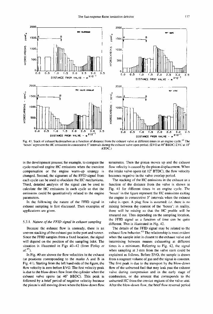
The fast-response flame ionization detector 117
2000 2000 _ l
lmC BLOUI~tN | Sin"
1500. B G A
c~ 500. o ~: ~_ 5oo.
I
0 . . . . 0 .0 0 . 5 .0 .5 .0 2 . 5 3 . 0 .5 0' .0 0 ' .5 1'.0 .5 2 ' .0 2 ' .5 3' .0 .5
DISTANCE FROM VALVE - m X l O - 1 DISTANCE FROM VALVE - mX10-1
2000 . . . . 2000
VALV£ OVlEIU..~ 90" ATI~
1500. B ,~ ~ 5oo a B ¼ i
o tip o
< : <
~ T
0 . 0 0 ' .5 1 ' .0 1 .5 2 ' .0 2 ' .5 3 ' .0 3 . 5 O 0 . 0 0 . 5 I .0 1 .5 2 . 0 2 ' .5 3' .0 3 . 5 DISTANCE FROII VALVE - m x I O - I DISTANCE FROM VALVE - m X I O - I
Fig. 41. Stack of exhaust hydrocarbon as a function of distance from the exhaust valve at different times in an engine cycle. 45 The 'boxes' represent the HC emissions in consecutive 5 ° intervals during the exhaust valve open period. (EVO at 46 ° BBDC; EVC at 18 °
ATDC.)
in the development process; for example, to compare the cycle-resolved engine HC emissions when the transient compensation or the engine warm-up strategy is changed. Second, the signature of the FFID signal from each cycle can be used to elucidate the HC mechanisms. Third, detailed analysis of the signal can be used to calculate the HC emissions in each cycle so that the emissions could be quantitatively related to the engine parameters.
In the following the nature of the FFID signal in exhaust sampling is first discussed. Then examples of applications are given.
5.3.1. Nature of the FFID signal in exhaust sampling
Because the exhaust flow is unsteady, there is an uneven stacking of the exhaust gas in the port and runner. Since the FFID samples from a fixed location, the signal will depend on the position of the sampling inlet. The situation is illustrated in Figs 40-42 (from Finlay et a l 45).
In Fig. 40 are shown the flow velocities in the exhaust (at positions corresponding to the marks A and B in Fig. 41 ). Starting from the left hand side of the figure, the flow velocity is zero before EVO. The first velocity peak is due to the blow-down flow from the cylinder when the exhaust valve opens (at 46 ° BBDC). This peak is followed by a brief period of negative velocity because the piston is still moving down when the blow-down flow
terminates. Then the piston moves up and the exhaust flow velocity is caused by the piston displacement. When the intake valve opens (at 12 ° BTDC), the flow velocity becomes negative in the valve overlap period.
The stacking of the HC emissions in the exhaust as a function of the distance from the valve is shown in Fig. 41 for different times in an engine cycle. The 'boxes' in the figure represent the HC emissions exiting the engine in consecutive 5 ° intervals when the exhaust valve is open. A plug flow is assumed: i.e. there is no mixing between the content of the 'boxes'; in reality, there will be mixing so that the HC profile will be smeared out. Thus depending on the sampling location, the FFID signal as a function of time can be quite different. This is illustrated in Fig. 42.
The details of the FFID signal may be related to the exllaust flow behavior. 45 The relationship is most evident when the sample inlet is closest to the exhaust valve and intermixing between masses exhausting at different times is a minimum. Referring to Fig. 42, the signal when sampling at 3 mm from the valve stem could be explained as follows. Before EVO, the sample is drawn from a stagnant volume of gas and the signal is constant. The first peak is due to the transport by the blow-down flow of the unburned fuel that may leak past the exhaust valve during compression and in the early stage of combustion, or the amount that corresponds to the unburned HC from the crevice regions of the valve seat. After the blow-down flow, the brief flow reversal period
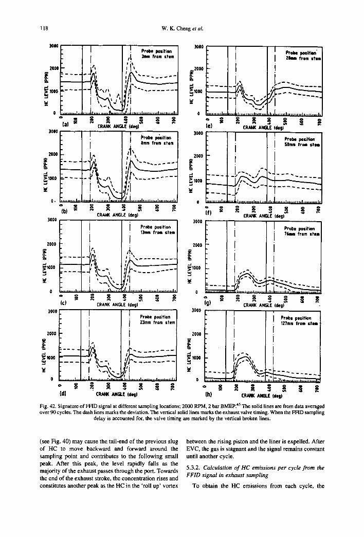
118 W.K. Cheng et al.
3000
2000 el
~1ooo
• I
I
i ""\~
! Probe position rL 3ira from stem
F'!4" ~, IL lllllhlllU,t lhllllu uh
O
Ca) ~ ]0o0 . I
i 2000 i,i,
~ 1000 , -
0~ 7 . . . . . . . . , . . . . . . . . . . . . . . . . ~ . . . . .
(b) "
3000
2000
1000 ~ ~ , . . . , . . j - - - - ~ t
( t )
CRAM( ANGLE Idogl I
I=robe position '. atom from stem
I . %
,.t!i ...... , ......... , ......... ,,,
CRANK ANGL! Ideg)
i i Probe position 13ram from stem
i I
:1~" . . . . . . . . . .
. / . . [ . . . . . . t . . . . . . . . .e . . . . . . . . . , .
3000 i
I
_2000 l = i L
..>.1000 - " ~ , , -- q t s
0 . . . . . . . . . , . . . . . . . l , . . . . . . . . . Z . . . .
3000
2000 ~2 a. ..-!. ~ I000
3000
2000
a.
~1ooo - - I
CRANK ANGLE (degl ?g)
l Probe position i 2)ram from stem
i
-_._-=_
Ii .|,11 Ii *l.*llh* *i hlllll1111 *
I Pr~lle position'-- i 20ml from stem
i
I h l [ l U l l l | l l l l h l l l l l l l l l l U l l l
3000: I
i 2000 i
~ P S. _
~ 1ooo - ~e
0 ~ . . . . . . . . , . . . e. . ~ . ** ~ ca)
° ~ (e)
i
Tf) *
i !
CRANK ANGLE Idql
I I position ! i Probe
I I so.,. fr,m stem I
CRANK ANGLE Idegl m
:rob~ ,~::~ tiX. .
I
i i I
O
( R N ~ ANGLE Ideg) (h) CRNqK ANGLE Idyll
CRANK ANGLE (deg)
I Probe position i 127mm from stem
i i
Fig. 42. Signature of FFID signal at different sampling locations; 2000 RPM, 2 bar 42 . BMEP. " The sohd lines are from data averaged over 90 cycles. The dash lines marks the deviation. The vertical solid lines marks the exhaust valve timing. When the FFID sampling
delay is accounted for, the valve timing are marked by the vertical broken lines.
(see Fig. 40) may cause the tail-end of the previous slug of HC to move backward and forward around the sampling point and contributes to the following small peak. After this peak, the level rapidly falls as the majority of the exhaust passes through the port. Towards the end of the exhaust stroke, the concentration rises and constitutes another peak as the HC in the 'roll up' vortex
between the rising piston and the liner is expelled. After EVC, the gas is stagnant and the signal remains constant until another cycle.
5.3.2. Calculation of HC emissions per cycle from the FFID signal in exhaust sampling
To obtain the HC emissions from each cycle, the
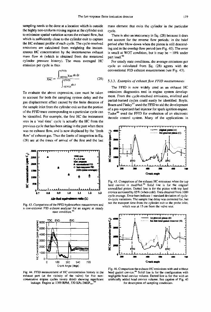
The fast-response flame ionization detector 119
sampling needs to be done at a location which is outside the highly non-uniform mixing region at the cylinder exit to minimize spatial variation across the exhaust flow, but which is sufficiently close to the cylinder exit to capture the HC exhaust profile of each cycle. The cycle-resolved emissions are calculated from weighting the instant- aneous HC concentration by the instantaneous exhaust mass flow rh (which is obtained from the measured cylinder pressure history). The mass averaged HC emission per cycle is thus
I t ( I V O )
t(EVO)XHcm dt XHC = ft(IVO) . (28)
J t(Evo)m t
To evaluate the above expression, care must be taken
to account for both the sampling system delay and the
gas displacement effect caused by the finite distance of
the sample inlet from the cylinder exit so that the portion
of the FHD trace corresponding to a particular cycle can
be identified. For example, the first HC the instrument
sees in a 'real time' cycle is actually the HC from the
previous cycle that has been sitting in the port when there
was no exhaust flow, and is now displaced by the 'fresh
flow' of exhaust gas. Thus the limits of integration in Eq.
(28) are at the times of arrival of the first and the last
3000 ' ' ' I . . . . I . . . . I . . . . I . . . . I . . . . . . .~
2300 •
" ° - ' o II=
: . . . . I , , , . I . . , , I , , , , I . . . . I , , . 0 0.7 0.8 0.9 1.0 1.1 1.2 1.3
,,,J)-f~ ~ nmo 0.)
Fig. 43. Comparison of the FFID hydrocarbon measurement and a conventional FID exhaust analyzer for an engine at steady
state condition. 46
mass element that exits the cylinder in the particular
cycle. There is also an inaccuracy in Eq. (28) because it does
not account for the reverse flow periods: in the brief period after blow-down when the piston is still descend- ing and in the overlap flow period (see Fig. 40). The error is small at WOT condition, but it may be - 1 0 % under part load. 46
For steady state conditions, the average emissions per cycle as calculated from Eq. (28) agrees with the conventional FID exhaust measurement (see Fig. 43).
~ 6000.:
t 5000.::
~ 4000.::
3000":
,ooo,: 0
I I
I
5.3.3. Examples of exhaust flow FFID measurements
The FFID is now widely used as an exhaust HC emissions diagnostics tool in engine system develop- ment. From the cycle-resolved emissions, misfired and partial-burned cycles could easily be identified. Boyle, Boam and Finlay 47 used the FFID to aid the development of a pre-vaporized fuel injector for spark ignition engine. Tudor 48 used the FFID for evaluation of an electronic throttle control system. Many of the applications in
( a c , , ~ W ) -
6 • 6
EVC
I I
I
) 180 360 540 720
Crank Angle (degs)
Fig. 44. FFtD measurement of HC concentration history in the exhaust port (at the vicinity of the valve) for five non- consecutive engine cycles (every third) showing significant
leakage. Engine at 1300 RPM, 330 KPa IMEP,et. 49
- i . , , , i , , , , i , , , , i , , , , i , , , , .
" od~m tC, moa (A) - ~,.a ~ ~ (c) -
, . . , I t . . . . i . . . . , . . L . f . , , ,
200 300 400 SN 600 ?O0
Cnmk
Fig. 45. Comparison of the exhaust HC emissions when the top land crevice is modified. ~ Solid line is for the original unmodified piston. Dotted line is for the piston with top land crevice increased by 85% (when cold). Data obtained from 1000 cycle average. Error bars indicate l standard deviation of cycle- to-cycle variations. The sample line delay was corrected for, but not the transport time from the cylinder exit to the probe inlet,
which was at 15 cm from the valve seat.
~ 4 0 N
L__
i- 1ooe
'1 ' ' ' ' I ' ' ' ' I ' ' ' " I . . . . I ' ' ' '
~ i t , , poovod i~=ao 0S) . . . . . . . . l ' o l l ~ s e l a m d p ~ r e m o v e d ( H )
i , , , [ i . . . . i . . . . i , , L , i . . . . 300 300 ~ dill0 6 O O
CnLuk a=Ele
Fig. 46. Comparison the exhaust HC emissions with and without head gasket crevice. 46 Solid line is for the configuration with negligible head crevice volume. Dotted line is for that with an artificially added head crevice volume. See caption of Fig. 45
for description of sampling conditions.
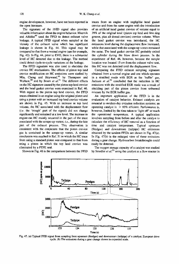
120 W.K. Cheng et al.
engine development, however, have not been reported in the open literature.
The signature of the FFID signal also provides valuable information about the engine behavior. Meernik and Alkidas 49 used the FFID to detect exhaust valve leakage. A typical FFID signal when sampled at the vicinity of the exhaust valve which has significant leakage is shown in Fig. 44. This signal may be compared to that from a normal engine (see for example, Fig. 42). In Fig. 44, prior to EVO, there is a substantial level of HC detected due to the leakage. The method could detect cycle-to-cycle variations of the leakage.
The FFID signature was also used to elucidate the crevice HC mechanisms. The effects of piston top land crevice modification on HC emissions were studied by Min, Cheng and Heywood, 46 by Thompson and Wallace, 5° and by Boam et al. 51 The different effects on the HC signature caused by the piston top land crevice and the head gasket crevice were examined in Ref. 46. With regard to the piston top land crevice, the FFID traces obtained in an engine using the original piston and using a piston with an increased top land crevice volume are shown in Fig. 45. With an increase in top land volume, the HC associated with the displacement flow (i.e. the 'trough' part of the signal) did not change significantly and remained at a low level. The increase in engine-out HC mainly occurred in the part of the trace associated with the scrape-up vortex; i.e., during the late part of the exhaust process. This observation is consistent with the conjecture that the piston crevice gas is contained in the scrape-up vortex. A similar conclusion was reached in Ref. 51 in which the HC trace from using a standard piston was compared to that from using a piston in which the top land crevice was eliminated by a PTFE seal.
Shown in Fig. 46 is the comparison between the FFID
traces from an engine with negligible head gasket crevice and from the same engine with the introduction of an artificial head gasket crevice of volume equal to 39% of the original total (piston top land and first ring groove, plus all thread crevices) crevice volume. When the head gasket crevice was introduced, the HC emissions level during the displacement flow increased, while that associated with the scrape-up vortex remained the same. The head gasket crevice HC probably exited the cylinder during the blow down process. In the experiment of Ref. 46, however, because the sample location was located 15 cm from the exhaust valve seat, this HC was not detected until the displacement flow.
Comparing the FFID exhaust sampling signature obtained from a normal engine and one which operates in a stratified mode with EGR as the 'buffer' gas, Jackson et al. s2 concluded that the reduction in HC emissions with the stratified EGR mode was a result of shielding part of the piston crevice from unburned mixture by the EGR buffer gas.
An important application of the FFID is in the evaluation of catalyst behavior. Exhaust catalysts are essential to modern-day emission reduction systems; an operating catalyst is > 95% efficient. Performance is, however, limited by the time taken to 'light off' or reach the operational temperature. A typical application involves sampling from before and after the catalyst to calculate the efficiency of HC removal as a function of time and catalyst temperature. Typical upstream (feedgas) and downstream (tailpipe) HC emissions obtained by the tandem FFIDs are shown in Fig. 47(a). In Fig. 47(b) is the enlarged view of these emissions during a gear change. Hydrocarbon breakthroughs could easily be detected.
The oxygen storage capacity of a catalyst was studied by Smedler et al. 53 using the catalyst as a flow reactor in
~ 10000
0 . . . .
0 40 80 120 160 200 Time (s) . . . . . . . .
- - 2000
133 134 135 136 137
Time (s)
Fig. 47. (a) Typical FF[D signal from sampling from upstream (feedgas) and downstream (tailpipe) of a catalyst; European drive cycle. (b) The emissions during a gear change shown in expanded scale.
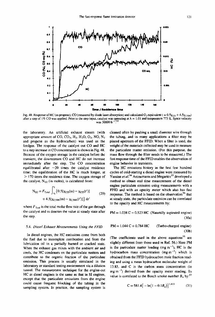
The fast-response flame ionization detector 121
I 0 . 0 ~
t1.9
0.11 11111
0.~
(~O.l O.Oll
O.d 0.0 I o u
0.1
0.~ O.a~l,
0.!
0 10 d4 04 O0 I N In IdO I40
l l m o I Jles idence l ime
Fig. 48. Response of HC (as propene), CO (measured by diode laser absorption) and calculated O2 equivalent ( = 0.5Xco + 4-SXc3r16) after a step of 1% CO was applied. Prior to the step input, catalyst was operating at X = 1.01 and temperature 773 K. Space velocity
was 30000 h-lk*
the laboratory. An artificial exhaust stream (with appropriate amount of CO, CO2, H2, H20, 02, NO, N2 and propene as the hydrocarbon) was used as the feedgas. The response of the catalyst out CO and HC to a step increase in CO concentration is shown in Fig. 48. Because of the oxygen storage in the catalyst before the transient, the downstream CO and HC do not increase immediately after the step. The CO concentration equilibrated after - 2 0 times the catalyst residence time; the equilibration of the HC is much longer, at > 170 times the residence time. The oxygen storage of
the catalyst, No2 (in moles), is calculated from:
No2 = FTotaJ f'ti, { O.5[Xco(SS)- Xco(t') ] (29)
+ 4.5[Xc3H6(SS ) -- XC3H6(/')] }d t '
where FTotal iS the total molar flow rate of the gas through the catalyst and ss denotes the value at steady state after the step.
cleaned often by pushing a small diameter wire through the tubing, and in many applications a filter may be placed upstream of the FFID. When a filter is used, the weight of the materials collected may be used to measure the particulate matter emission. (For this purpose, the mass flow through the filter needs to be measured.) The fast response time of the FFID enables the observation of engine behavior in transients.
The HC emissions history in the first few hundred cycles of cold-starting a diesel engine were measured by Yassine et al. 54 Arcoumanis and Megaritis 55 developed a method to obtain real time measurement of the diesel engine particulate emission using measurements with a FFID and with an opacity meter which also has fast response. The method is based on the observation 56 that at steady state, the particulate emission can be correlated to the opacity and HC measurements by:
PM = i.038 C + 0.523 HC (Naturally aspirated engine)
(30a)
5.4. Diesel Exhaust Measurements Using the FFID
In diesel engines, the HC emissions come from both the fuel due to incomplete combustion and from the lubrication oil in a partially burned or cracked state. When the exhaust gas mixes with the ambient air and cools, the HC condenses on the particulate matters and contribute to the organic fraction of the particulate emission. This process is usually simulated in the laboratory or standard testing environment via a dilution tunnel. The measurement technique for the engine-out HC in diesel engines is the same as that in SI engines, except that the particulate emissions from the engine could cause frequent blocking of the tubing in the sampling system. In practice, the sampling system is
PM = !.044 C + 0.784 HC (Turbo-charged engine)
(30b)
(The coefficients used in the above equations 55 are
slightly different from those used in Ref. 56.) Here PM is the particulate matter loading (mg m-3), HC is the hydrocarbon mass concentration (mg m -3) which is
obtained from the FFID hydrocarbon mole fraction read- ing and using a mean hydrocarbon molecular weight of 13.85, and C is the carbon mass concentration (in mg m -3) derived from the opacity meter reading. Its value is correlated to the Bosch smoke number Bn by: 57
C = 5 8 1 . 4 [ - I n ( l - 0. lBn)] 1'413 (31)
122 W.K. Cheng et al.
The relationship between Bosch number and opacity
meter reading is given in Ref. 58. Arcoumanis and Megaritis 55 applied the steady state
correlation (Eq. (30)) to the instantaneous FFID and opacity meter data for step transients in speed and load in a diesel engine. They compared the cumulative particu- late emissions calculated from these data and the amount collected on a filter in the diluted exhaust. The agreement was within 20% for all the test cases; thus the comparison lends support to the validity of using steady state correlation of Eq. (30) for the transient data.
6. C O N C L U D I N G REMARKS
The fast-response flame ionization detector (FFID) was in use for almost a decade and has become an important diagnostic tool for analyzing hydrocarbon emissions from internal combustion engines. The fast response of the instrument (time constant of a few millisecond) enables it to be used in the studying of the unsteady engine processes both within a cycle and from cycle to cycle. This review summarizes the principle and properties of the FFID, especially the sampling system which isolates the pressure pulsation at the sample inlet from the ionization detector so that an unambiguous hydrocarbon measurement could be made. Then prac- tical working experience and application examples are given to illustrate the versatility of the instrument. The scope of the review was limited to engine applications so that other important usage of the instrument is not covered; for example, in using the FFID as a detector of hydrocarbon released as a tracer to study the dispersion and transport process in the atmosphere or in piping systems. The purpose of the review is to give a tutorial on the FFID and to document its behavior so that the users can obtain a comprehensive understanding of the instrument. Though the FFID is a complex device, we expect that with increasing usage, the users will gain sufficient familiarity with it to regard it as a 'standard' piece of equipment.
Acknowledgements--In writing this article, W.C. was partially supported by an Industrial Consortium on Engine and Fuels Research; the member companies are" Chrysler Corp., Ford Motor Co., GM Corp., Peugeot S.A., Regie Nationale des Usines Renault, Shell Development Co., Shell Research Ltd., and the Volvo Car Corp. T.S. was partially supported by the Engineering and Physical Sciences Research Council, U.K., Ford Motor Co., U.K, and Darwin College, Cambridge University. N.C. was partially supported by Ford Mortor Co., U.K., Cambustion, Ltd.
N O M E N C L A T U R E
A Tube cross-section area ( = ~rd2/4) aT Isothermal sound speed ( = ~(RT)) Bn Bosch smoke number C Concentration d Tube diameter
D Molecular diffusivity f Pipe flow friction factor; see Eq. (9) HC Hydrocarbons K Effective longitudinal diffusivity for Taylor
diffusion L Tube length L* Extent of backflow of burned gas into the intake
port rh Mass flow rate OF Valve overlap factor; see caption of Fig. 35 for
definition P Pressure Pc ' Pressure at the constant-pressure chamber Pi Sample inlet pressure of FFID PM Particulate matter 6Pc Fluctuation of CP chamber pressure z~P Pressure difference across the tube P* Downstream pressure at choking R Gas constant Re Reynolds number based on the tube diameter RPM Revolution per minute rc Compression ratio s Entropy Sc Schmidt number ( = D/I~)
t Time T Temperature u Velocity, mass averaged over flow cross-section u 1 Entrance velocity V CP chamber volume x distance Xr Residual gas fraction p Density o Parameter describing the width (in time) of the
weighting function for signal averaging by laminar Taylor diffusion; see Appendix B.
¢ Fuel/air equivalence ratio
¢* HC equivalence ratio; = XHC/XHC; stoichiometric, no
residual)
rc Integrating time constant as a result of Taylor diffusion along the tube
rt Transit time t~ Viscosity Xco Carbon monoxide mole fraction XHC Hydrocarbon mole fraction
REFERENCES
1. The Federal Clean Air Act, Title II, Public Law 101-549, amended November, 1990; the Low Emissions Vehicle/ Clean Fuels Program, approved by the California Air Resources Board, September 1990.
2. Sternberg, J.C., Gallaway, W.S. and Jones, D.T., The Mechanism of Response of Flame Ionization Detectors, in Gas Chromatography, eds N. Brenner, J.E. Callen and M.D. Weiss, Academic Press, New York, pp. 231-267 (1962).
3. McWilliam, I.G. and Dewar, R.A., Nature, 1958, 181,760. 4. Calcote, H.F., 8th Symposium (Int.) on Combustion, pp.
184-199 (1960). 5. Miller, W., 14th Symposium (Int.) on Combustion, pp. 307-
320 (1976). 6. Lawton, J. and Weinberg, F., Electrical Aspect on
Combustion, Clarendon Press, Oxford (1969).
The fast-response flame ionization detector 123
7. Baulch, D.L., Cobos, C.J., Cox, R.A., Frank, P., Hayman, G., Just, Th., Kerr, J.A., Murrells, T., Pilling, M.J., Troe, J., Walker, R.W. and Warnatz, J., Combustion and Flame, 1994, 98, 59-79.
8. Green, J.A. and Sugden, T.M., 9th Symposium (int.) on Combustion, pp. 607-621 (1962).
9. Perkins, G. Jr., Rouayheb, G.M., Lively, L.D. and Hamilton, W.C., Response of the gas chromatographic flame ionization detector to different functional groups, in Gas Chromatography, eds N. Brenner, J.E. Callen and M.D. Weiss, Academic Press, New York, pp. 231-267 (1962).
10. Ettre, LS., Relative response of hydrocarbons on the ionization detectors, in Gas Chromatography, eds N. Brenner, J.E. Callen and M.D. Weiss, Academic Press, New York, pp. 231-267 (1962).
11. Ettre, L.S., J. Chromatog., 1962, 8, 525-530. 12. Jackson, M.W., J. APCA, 1966, 16 (12), 697-702. 13. Fackrell, J.E., J. of Physics E, 1980, 13, 888-893. 14. Collings, N., SAE Paper 871691 (1987). 15. Collings, N., SAE Paper 880316 (1988). 16. Collings, N., SAE Paper 880517 (1988). 17. Cheng, W.K., Galliot, F. and Collings, N., SAE Trans-
action, 98, No.3, Paper 890579, pp. 1083-1090 (1989). 18. White, F., Fluid Mechanics, 2nd Ed., McGraw-Hill (1986). 19. Summers, T., Fast-response FID measurement of SI engine
residual gas hydrocarbon concentration, Ph.D. Thesis, Engineering Dept., Cambridge University, Cambridge, U.K. (1996).
20. Peckham, M.S., Study of engine wall layer hydrocarbons with a fast response FID, Ph.D. Thesis, Engineering Dept., Cambridge University, UK (1993).
21. Crocco, L., One dimensional treatment of steady gas dynamics, in Fundamentals of Gas Dynamics, Vol. 3 of High Speed Aerodynamics and Jet Propulsion, Princeton University Press (1958).
22. Summers, T. and Collings, N., SAE Transaction, 104, No. 3, Paper 950160, pp. 99-113 (1995).
23. Taylor, G.I., Proceed. of the Royal Soc. of London, 1954, 219, 186-203.
24. Taylor, G.I., Proceed. of the Royal Soc. of London, 1954, 223, 446-468.
25. Smith, R., J. Fluid Mech., 1989, 208, 25-43. 26. Fox, J.W., Min, K.D., Cheng, W.K. and Heywood, J.B.,
SAE Transaction, 101, No. 4, Paper 922170, pp. 1088- 1099 (1992).
27. Ginesi, D., Grebe, G., Chemical Engineering, June, 103 (1987).
28. Summers, T. and Collings, N., SAE Transaction, 104, No. 4, Paper 952541, pp. 2479-2495 (1995).
29. Galliot, F., Cheng, W.K., Cheng, C.O., Sztenderowicz, M., Heywood, J.B. and Collings, N., SAE Transaction, 99, No. 3, Paper 900485, pp. 1144-1150 (1990).
30. Ladommatos, N., J. Inst. of Energy, 1992, 65, 94-101. 31. Crawford, J.G. and Wallace, J.S., SAE Paper 961201
(1996). 32. Cheng, C.O., Cheng, W.K., Heywood, J.B., Maroteaux, D,
and Collings, N., SAE Transaction, 100, No. 3, Paper 912401, pp. 1839-1851 (1991).
33. Shin, Y., Min, K. and Cheng, W.K., SAE Transaction, 104, No. 3, Paper 952481, pp. 1544-1553 (1995).
34. Schurov, S. and Collings, N., SAE Transaction, 104, No. 3, Paper 952485, pp. 1554-1563 (1995).
35. Cheng, W.K., Hamrin, D., Heywood, J.B., Hochgreb, S., Min, K. and Norris, M., SAE Transaction, 102, Paper 932708, pp. 1207-1220 (1993).
36. Sleightmore, G.R., SAE Transaction, 99, No. 3, Paper 900484, pp. 1124-1143 (1990).
37. Meyer, R.C. and Thring, R.H., SAE Paper 950069 (1995). 38. Abata, D. and Wellenkotter, K., SAE Paper 920423 (1992). 39. Rose, D., Ladommatos, N. and Stone, R., SAE Transaction,
103, No. 3, Paper 940382, pp. 506-519 (1994). 40. Fox, J.W., Cheng, W.K. and Heywood, J.B., SAE
Transaction, 102, No.3, Paper 931025, pp. 1538-1544 (1993).
41. Peekham, M. and Collings, N., SAE Paper 922237 (1992). 42. Peckham, M. and Collings, N., SAE Paper 932642 (1992). 43. Peckham, M. and Collings, N., SAE Paper 932643 (1992). 44. Green, R., SAE Paper 970823 (1997). 45. Finlay, I.C., Boam, D.J., Bingham, J.F. and Clark, T.A.,
SAE Paper 902165 (1990). 46. Min, K., Cheng, W.K. and Heywood, J.B., SAE Trans-
action, 103, No. 3, Paper 940306, pp. 371-385 (1994). 47. Boyle, R.J., Boam, D.J. and Finlay, I.C., SAE Transaction,
102, No. 3, Paper 930710, pp. 949-957 (1993). 48. Tudor, R.J., SAE Paper 930939 (1993). 49. Meemik, P.R. and AIkidas, A.C., SAE Transaction, 102,
No. 4, Paper 932752 pp. 1470-1478 (1993). 50. Thompson, N. and Wallace, J.C., SAE Paper 940480
(1994). 51. Boam, D.J., Finlay, I.C., Biddulph, T.W., Ma, T., Lee, R.,
Richardson, S.H., Bloomfield, J., Green, J.A., Wallace, S., Woods, W.A. and Brown, P., Proc. L Mech. E., C448/064 (1992).
52. Jackson, N.S., Stokes, J., Lake, T.H., Sapsfor, S.M., Heikal, M. and Denbratt, I., SAE Paper 960837 (1996).
53. Smedler, G., Eriksson, S., Lindblad, M., Bernier, H, Lundgren, S. and Jobson, E., SAE Transaction, 102, No. 4, Paper 930944, pp. 671-682 (1993).
54. Yassine, M.K., Tagomori, M.K., Henein, N.A. and Bryzik, W., SAE Paper 960249 (1996).
55. Arcoumanis, C. and Megaritis, A., SAE Transaction, 101, No. 4, Paper 922390, pp. 1966-1976 (1992).
56. Green, G. and Wang, C.H.T., SAE Paper 810260 (1981). 57. Alkidas, A., SAE Transaction, 93, Paper 840412 (1984). 58. Green, G.L. and Wallace, D., SAE Transaction 89(4), Paper
801373 (1980).
APPENDIX A
Response of flame ionization detector to different
compounds; response normalized using n-heptane ----
7.0. Data from Refs. 2, 9 and 10. Repeated values are
from different sources.
Family Compound Carbon atoms Normalized in molecule response
Alkanes methane 1 1.02 methane 1 0.9 ethane 2 1.98 ethane 2 1.89 propane 3 2.98 propane 3 2.84 n-butane 4 3.78 2-M propane 4 3.78 n-pentane 5 4.94 n-pentane 5 5.24 2-M butane 5 5.29 iso-pentane 5 4.69 n-hexane 6 5.98 n-hexane 6 6.20 2-3-dM butane 6 6.20 2-2-dM-butane 6 6.13 3-M-pentane 6 6.26 2-M-pentane 6 6.32 n-heptane 7 7.00 2-3-dM-pentane 7 6.93 2-M-hexane 7 7.14 3-M-hexane 7 7.14 2,2-dM pentane 7 7.14 2,4-dM pentane 7 7.14 3,3-dM pentane 7 7.21
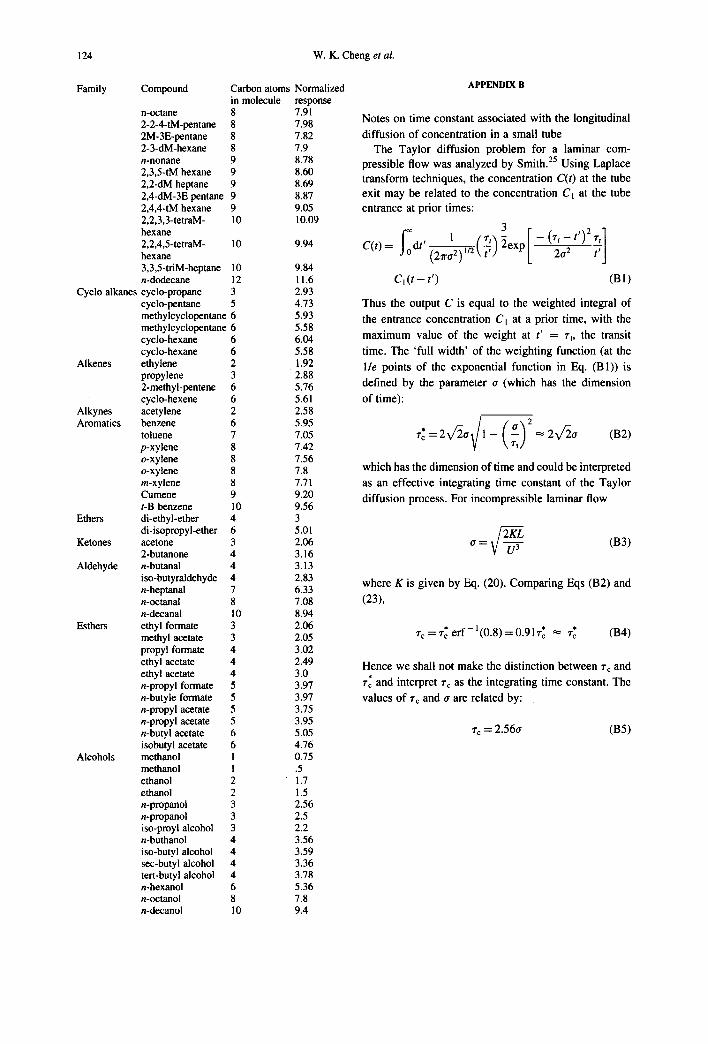
124 W.K. Cheng et aL
Family Compound Carbon atoms Normalized in molecule response
n-octane 8 7.91 2-2-4-tM-pentane 8 7.98 2M-3E-pentane 8 7.82 2-3-dM-hexane 8 7.9 n-nonane 9 8.78 2,3,5-tM bexane 9 8.60 2,2-dM heptane 9 8.69 2,4-dM-3E pentane 9 8.87 2,4,4-tM hexane 9 9.05 2,2,3,3-tetraM- 10 10.09 hexane 2,2,4,5-tetraM- 10 9.94 hexane 3,3,5-triM-heptane 10 9.84 n-dodecane 12 11.6
Cyclo alkanes cyclo-propane 3 2.93 cyclo-pentane 5 4.73 methylcyclopentane 6 5.93 methylcyclopentane 6 5.58 cyclo-hexane 6 6.04 cyclo-hexane 6 5.58
Alkenes ethylene 2 1.92 propylene 3 2.88 2-methyl-pentene 6 5.76 cyclo-hexene 6 5.61
Alkynes acetylene 2 2.58 Aromatics benzene 6 5.95
toluene 7 7.05 p-xylene 8 7.42 o-xytene 8 7.56 o-xylene 8 7.8 m-xylene 8 7.71 Cumene 9 9.20 t-B benzene 10 9.56
Ethers di-ethyl-ether 4 3 di-isopropyl-ether 6 5.01
Ketones acetone 3 2.06 2-butanone 4 3.16
Aldehyde n-butanal 4 3.13 iso-butyraldehyde 4 2.83 n-heptanal 7 6.33 n-octanal 8 7.08 n-decanal 10 8.94
Esthers ethyl formate 3 2.06 methyl acetate 3 2.05 propyl formate 4 3.02 ethyl acetate 4 2.49 ethyl acetate 4 3.0 n-propyl formate 5 3.97 n-butyle formate 5 3.97 n-propyl acetate 5 3.75 n-propyl acetate 5 3.95 n-butyl acetate 6 5.05 isobutyl acetate 6 4.76
Alcohols methanol 1 0.75 methanol 1 .5 ethanol 2 1.7 ethanol 2 1.5 n-pmpanol 3 2.56 n-propanol 3 2.5 iso-proyl alcohol 3 2.2 n-buthanol 4 3.56 iso-butyl alcohol 4 3.59 sec-butyl alcohol 4 3.36 tert-butyl alcohol 4 3.78 n-bexanol 6 5.36 n-octanol 8 7.8 n-decanol 10 9.4
APPENDIX B
Notes on time constant associated with the longitudinal
diffusion of concentration in a small tube The Taylor diffusion problem for a laminar com-
pressible flow was analyzed by Smith. 25 Using Laplace transform techniques, the concentration C(t) at the tube exit may be related to the concentration C~ at the tube entrance at prior times:
3
1 2exp I C(t) = I0d t ' (21ra2) ~ 7 J
C l ( t - t ' ) (BI)
Thus the output C is equal to the weighted integral of
the entrance concentration C~ at a prior time, with the
maximum value of the weight at t' = rt, the transit
time. The 'full width' of the weighting function (at the
lie points of the exponential function in Eq. (B1)) is
defined by the parameter ~r (which has the dimension
of time):
rc = 2X/~o 1 - = 2X/2o (B2)
which has the dimension of time and could be interpreted
as an effective integrating time constant of the Taylor
diffusion process. For incompressible laminar flow
2 ~ (B3) ° = w U 3
where K is given by Eq. (20). Comparing Eqs (B2) and
(23),
* - - 1 * * rc = re eft (0.8) = 0.91 rc ~-- rc (B4)
Hence we shall not make the distinction between rc and
r~ and interpret rc as the integrating time constant. The
values of rc and o are related by:
re = 2.560 (B5)