THE FAMA-MACBETH APPROACH REVISITED - Ross School of Business

1

THE FAMA-MACBETH APPROACH REVISITED

By

Paolo Pasquariello

Ph-D Candidate – New York University – Stern School of Business

Summary The three-step approach devised by Fama and MacBeth (1973) survived most of the empirical results of their paper to become a standard methodology in the financial literature for its undeniable merits of simplicity and clarity. Nonetheless, their procedure fails to properly account for estimation errors and lack of independence among cross-sectional residuals. This uncertainty may lead to false inference, when simple t-statistics are calculated to empirically validate or disprove hypothesis based on the estimated parameters. In this paper we propose a multi-step econometric methodology that attempts to control for the main drawbacks of the FM technology and mitigates the sensitivity of any analysis of CAPM implications to the choice of a proxy for the market portfolio, as suggested by Kandel & Stambaugh (1995). The procedure is based on the work by McElroy & Burmeister (1988) and is developed around a Bilinear version of the CAPM following the early contribution of Brown & Weinstein (1983). We apply two versions of the new approach to the same set of data originally employed by Fama and MacBeth in their analysis of the two-parameter Sharpe-Lintner model. The new resulting empirical evidence leads us to the conclusion that, although there seems to be on average a positive trade-off between return and risk over the time frame 1926-1968, nonlinearities and non-beta measures of risk play a very important and apparently systematic role in explaining the cross-sectional variability of excess returns. [This version, August 1999]

2

1. Introduction

Fama-MacBeth (FM) (1973) represents a landmark contribution toward the empirical

validation or refusal of the basic implications of the Capital Asset Pricing Model. A

relevant portion of the available financial literature, see for example the remarkable work

by Roll (1977), devoted its attention to the issue of determining the mean-variance

efficiency of the market portfolio. FM first interpreted the CAPM as implying a basic

linear relationship between stock returns and market betas which should completely

explain the cross-section of returns at a specific point in time.

In order to test the effectiveness of the CAPM in justifying that observed cross-sectional

variability of returns, FM designed and implemented a basic two-step regression

methodology that eventually survived the first set of empirical results that it generated, to

become a standard approach in the field.

In this paper, we attempt to provide detailed answers to three main questions arising from

the analysis of FM’s work. First, are the model specification they adopted and the two-

step estimation technique they elaborated exempt from statistical and economic critique?

Second, if the answer to the first question is negative, is it possible to attack the general

FM problem with different tools whose results are immune from some of the flaws of

their procedure? Last, but not least, do the estimates obtained with new and apparently

more reliable econometric work confirm or deny some of the general conclusions of their

analysis?

The next paragraph describes briefly the FM paradigm, and provides a replication of their

main empirical findings. Paragraph 3 focuses on the problems in the FM technique that

the current financial literature has identified as affecting the statistical reliability of their

results, and provides a (partially) new methodology to account for them. Paragraph 4

presents an application of this approach to the same set of data originally used by Fama

and MacBeth. Paragraph 5 concludes.

2. Fama-MacBeth: a Replication

The basic theoretical claim described in FM and resulting from the Sharpe-Lintner

version of the CAPM simply states that variability in market betas accounts for a

significant portion of the cross-sectional variability of stock returns at a certain point in

3

time, or for a specified sample period. In order to make this proposition empirically

testable the authors describe the following stochastic model for returns:

Assuming that the betas are known, equation [1] and [2] are generalized into:

where S(i) represents the standard deviation of residual returns ε(i) for security i, for i =

1,…..,n. From equation [3] FM are able to test some of the major implications of the

CAPM simply through basic statistical analysis of the estimates for the various γs, under

the assumption that both the returns and (consequently) the parameters describing their

stochastic process are normally distributed and temporally IID. Indeed, this assumption

allows the construction of simple t-test for the following set of hypothesis:

Hypothesis C1 to C3 specify, to paraphrase FM, the general expected return implications

of the two-parameter model described in equations [1] and [2], as they suggest that

investors hold efficient portfolios and the market portfolio itself is efficient. The SL

hypothesis is simply an attempt to verify whether a very specific two-parameter model

describing market equilibrium is consistent with the empirical data. As such, its refusal

does not affect any of the more general, hence more interesting, assumptions regarding

[ ]R R

E R E R E R E Rit i mt it

i f i m f

= + +

= + −

γ β ε

β0 [ 1 ]

[ 2 ]( ) ( ) ( ) ( )

R Sit t t i t i t i it= + + + +γ γ β γ β γ η0 1 22

3 [ 3 ]

[ ]

[ ]

[ ] [ ] [ ][ ]

C1 - Linearity C2 - No Systematic Effect

of Non - Beta Risk C3 - Positive Expected

Return - Risk Trade - off

SL - Sharpe - Lintner CAPM ME - Market Efficiency all the stochastic coefficients and the disturbances are " fair games"

H E

H E

H E E R E R

H E R

t

t

t mt ft

t ft

it

0 2

0 3

0 1

0 0

0

0

0

: �

: �

: �

: �

�

γ

γ

γ

γ

η

=

=

= − >

=

4

the asserted validity of the CAPM in explaining the cross-section variability of equity

returns. ME is a “not-strong” form proposition of capital markets’ efficiency, and

originates from the CAPM assumption that markets are perfect, in the sense that stock

prices reflect all publicly available information at any specific point in time. This in turn

implies that the observation of past values of the estimated parameters γs should not lead

to non-zero future estimates of the risk premium, the impact of non-linearities and the

return disturbances. Nonetheless, this argument does not appear to be convincing, and it

did not receive additional attention from the subsequent literature, for it ignores the fact

that serial correlation for the resulting estimates may result from the way the estimators

are constructed and the stock return data are collected, and not from presumed market

inefficiencies. Moreover, the impact of those effects is by itself not easily quantifiable.

Consequently, in this paper we focus on C1-C3 as the main object of FM analysis and of

our subsequent empirical investigation.

The empirical implementation of this approach involves the following three-step

procedure:

Step 1

Equation [1] is estimated for each of the stocks in the sample;

Step 2

Assuming that the betas resulting from step 1 are given, cross-sectional OLS regressions

[3] are run for each of the available dates, and time series of the parameters’ estimates are

consequently generated;

Step 3

The time series for the γs are analyzed and tests for C1-C3 are performed using simple t-

test statistics.

5

The data utilized by FM for this study are monthly percentage returns1 for all common

stocks traded on the New York Stock Exchange (NYSE) during the period going from

January 1926 to June 1968, as recorded by the Center for Research in Security Prices of

the University of Chicago.

The Market return Rm(t) is the “Fisher’s Arithmetic Index”, i.e. an equally weighted

average of the returns on all stocks listed on the NYSE in month t. The risk-free rate Rf(t)

is calculated from the average Street Convention quoted yield reported in the Fama-Bliss

Database for 1-month Treasury Bills from January 1926 to June 1968, according to the

following formula:

As stated in step 2, the cross-sectional regressions of equation [3] run under the strong

assumption that the estimated betas deriving from step 1 correspond to the true and

unknown market betas. This choice unavoidably introduces an “error-in-variable”

complication: the efficiency and consistency of the resulting estimates for the parameters

are going to be negatively affected by the degree of uncertainty related to the

supposedly known regressors in [3].

FM cope with this issue by aggregating the available stocks into beta-portfolios in order

to increase the precision of the resulting beta estimates. The sample period 1926-1968 is

divided into 9 subsets, as described in Table 1. Each subset is in turn segmented into

three non-overlapping sub-periods. Individual stocks’ betas are estimated during the first

one, and stocks are subsequently ranked according to those estimates. Then, 20 portfolios

are created by grouping the stocks by the beta ranking. Portfolio betas are calculated for

each month of the second (“estimation”) sub-period. Finally, cross-sectional regression

1 Including dividends and capital gains, with the appropriate adjustment for capital changes, such as splits

and stock dividends. In the appendix, we report the sample Fortran code used to retrieve the needed data.

PD

R

RP D

R R

t AVG tStreet

ftAnnual

t

ft ftAnnual

100360

1001

365

1 1112

, D = duration, in days

6

equations [3] are estimated and time-series for the resulting parameter-estimates are

derived for every month of the final sub-period.

The attached formula sheets in the appendix describe precisely all the procedures and the

formulas adopted for the derivation of the γs. Table 2 reports the betas and related sample

statistics resulting from four selected estimation periods. As evident from the last row of

each of the sub-period tables, the standard errors of the portfolio betas are one-third to

one-seventh the standard errors of the individual betas. The gain in precision seems

evident2.

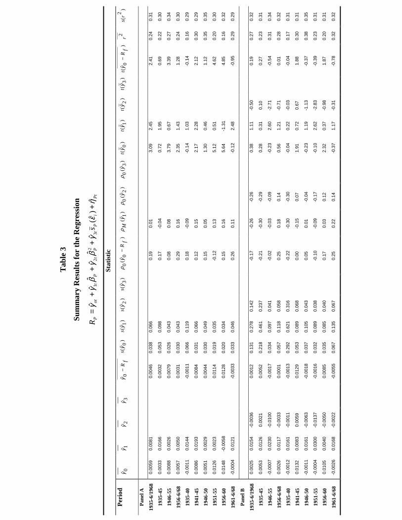
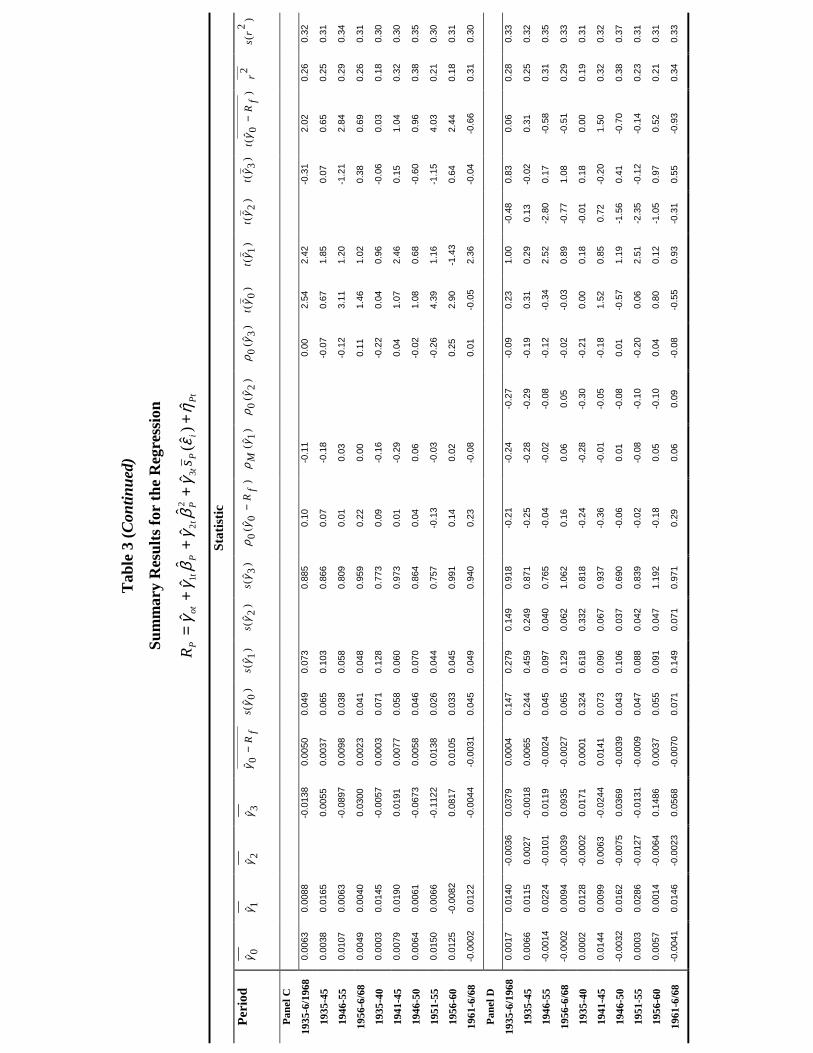
Table 3 reports summary results and test statistics for each of the following four panels

for the cross-sectional regressions:

The last panel, D, corresponds to equation [3]. Table 3 contains the major tests of the

implications of the two-parameter models. Results are there presented for 10 periods, the

overall sample 1926-1968, three long sub-periods, 1935-1945, 1946-1955, 1956-1968,

and six short subperiods which, with the exception of the first, cover 5 years each. The

estimates from panel B and D do not seem to reject the hypothesis formulated in C1 that

the relationship between expected return and beta is linear. The t-statistics reported for

the coefficient γ2 leads us to the conclusion that the estimated parameter is not

significantly different from zero in a statistical sense. The values of t(γ2) for the overall

period 1935-1968 in panels B and D are just –0.50 and –0.48 respectively, and remain

“small” for significance levels above 75% for most of the considered sub-samples. For

the long subset 1946-1955 the t-statistics are instead –2.71 and –2.80. However, this

seems to be resulting from a specific time-period, 1951-1955, where in fact the t-values

are again significant.

2 Evident but not sufficient, as we will emphasize and explore more carefully in the next paragraph.

PANEL A

PANEL B

PANEL C

PANEL D

R

R

R S

R S

Pt t t Pt Pt

Pt t t Pt t Pt Pt

Pt t t Pt t P i Pt

Pt t t Pt t Pt t P i Pt

= + +

= + + +

= + + +

= + + + +

� � � �

� � � � � �

� � � � ( � ) �

� � � � � � ( � ) �

γ γ β η

γ γ β γ β η

γ γ β γ ε η

γ γ β γ β γ ε η

0 1

0 1 22

0 1 3

0 1 22

3

7

The statistic t(γ3) in Panels C and D in table 3 also allows us not to reject C2: the devised

measure of risk, in addition to beta, does not affect expected returns in any of the sub-

periods there examined, for the values of the t-test are small and randomly positive and

negative.

Although satisfactorily for the two-parameter model, the results obtained so far would be

vain if the most critical hypothesis still to analyze, C3, had to be rejected. This would in

turn imply that the available data do not sustain the fundamental assumption that there is

on average a positive trade-off between risk and return. Fortunately for the believers of

the CAPM, this seems to be the case, at least for panels A and C. The results are

somehow mixed for panels B and D, where the model offers a statistically meaningful

representation of the data for just some of the sub-samples considered in the analysis. FM

claim that small t-statistics for most of those sub-periods reflect the <<……substantial

month-to-month variability of the parameters of the risk-return regressions… >>3. We

argue instead, as it will be explained more precisely in the next paragraph, that the

estimators resulting from their three-step approach are consistent but not efficient. It is

this lack of efficiency, materializing in higher standard errors of the resulting estimates,

not simply the variability of the estimates of the model of equation [1], to generate

smaller t-statistics for the hypothesis we are testing.

The behavior of the time series for the estimated γ1, γ2, and γ3 is consistent with the ME

hypothesis that the capital markets are efficient. As evident from the ρ columns in table

3, the serial correlations for each of the three parameters are generally low both in terms

of explanatory power and statistical significance.

Table 4 offers a perspective on the behavior of the market during each of the sub-periods

under examination, and on the empirical validation of the two-parameter Sharpe-Lintner

model. If their version of the CAPM were correct, then we would expect the estimated

value for the average γ0 to be statistically close to the expected return on any zero-beta

security or portfolio, and the excess market return to be statistically close to γ1. However,

just in two of the considered samples, 1935-1940 and 1961-1968, Rm(t) – Rf(t) is similar

to the corresponding γ1. This appears to be a consequence of the average risk-free rate

3 Fama-MacBeth (1973), page 624.

8

being smaller than the average γ0. FM observe that the most efficient test for the SL

hypothesis is provided by the results of panel A, as the standard error of the resulting

estimates for the constant coefficient of the cross-sectional regressions of equation [3] are

substantially lower than their counterparts in panels B to D. Nonetheless, except for the

earliest and the latest periods (1935-45 and 1961-1968), the values of t(γ0 - Rf) are large,

thus leading us to reject the Sharpe-Lintner version of the CAPM4.

Finally, Table 5 reports an attempt by FM to account for the proportion of the variability

of the values obtained for the γs that is potentially explained by estimation errors, or in

other words by lack of precision of the coefficient estimates used to analyze the two-

parameter model, rather than by the variability of the underlying and unobserved true

parameters. The authors construct an F-test for the null hypothesis that the estimation

error is big, i.e. that the sample variance of the month-by-month estimated γs is equal to

the variance of the estimation error. The resulting F values listed in table 5 for each of the

four panels are generally small (except for panel A). This suggests that the reliability of

the estimates for the γs declines considerably when non-linearity and non-beta risk

factors are included in the cross-sectional regressions of equation [3].

In short, given the assumption that the adopted proxy for the market portfolio is efficient,

FM’s results appear to support the hypothesis that the pricing of securities in the sample

period 1935-1968 is in line with most of the implications of the two-parameter model for

expected returns. Specifically, the data confirm the existence of a positive trade-off

between risk and return, that on average nonlinearity effects are zero and that non-beta

risk factors do not have additional explanatory power for the cross-sectional variability of

returns, when beta has been properly accounted for. More ambiguous are the results for

the specific Sharpe-Lintner version of the CAPM adopted as basic theoretical framework.

Nonetheless, the issue of determining the precision of the estimates for the parameters of

interest in the model proposed by Fama and MacBeth affects the conclusions we derive

4 It is interesting to observe that the SL version of the CAPM seems to hold for the quadratic model of

panel B and the enlarged version of panel D. However, this last case appears to be largely influenced by the

presence of the quadratic term and not by the non-beta risk term, for which the rejection of the SL

hypothesis is strong in panel C. These considerations make the testing of the two-parameter approach more

ambiguous.

9

from the analysis of their major results. Can we devise an estimation procedure that

attempts to control for and maximizes the degree of precision involved in the cross-

sectional regressions for panels A to D by generating efficient estimates of the parameters

of interest? The next paragraph is devoted to provide a satisfactory answer to this

compelling question.

3. A Multi-Step approach to Gamma Estimation

The Fama-MacBeth methodology has become a standard for the estimation and testing of

different versions of the CAPM and the APT model of Ross. Their three-step sequence

for the estimation of factor-loadings and factor-prices revealed to be especially effective

for multi-factor models, as it can easily be modified to accommodate additional non-beta

measures of risk. Nonetheless, as briefly emphasized in paragraph 2, the FM approach is

affected by three major problems, that eventually weaken many of the conclusions that

may result from its practical application to financial data:

a) Errors-In-Variable Problem: the cross-sectional regressions defined in

equation [3] are based on the assumption that the betas are given, i.e. that the

betas resulting from the basic model of equation [1] correspond to the true and

unobservable market betas. The resulting and unavoidable errors in generating

the needed beta-risk factor affect the precision by which the parameters of the

cross-sectional regressions are estimated, hence the validity of the conclusions

that may be derived from those estimates.

b) Cross-Sectional Independence Problem: in estimating the cross-sectional

model of panels A to D through OLS, FM implicitly assume that the variance-

covariance matrix of the residuals η at each point in time t is proportional to a

diagonal matrix. This choice, when not adequately supported by the actual

data, makes the resulting estimates for γs consistent but not efficient.

Consequently, the t-statistics for these parameters may lead to false inference

about the hypothesis under examination.

c) The Roll Critique: the true market portfolio is unobservable, and the proxy

used for the market return is not necessarily mean-variance efficient. If this is

10

the case, then, as masterly emphasized by Roll (1977) and Roll and Ross

(1994), evidence of the lack of a relation (or instead of a strong relation)

between expected return and beta may be resulting from the adoption of the

wrong proxy, rather then from the validity of the underlying theory. This

happens because, if the true market portfolio is mean-variance efficient, the

cross-sectional relationship between expected returns and betas reveals to be

very sensitive to even small deviations of the true market portfolio from the

proxy adopted for the empirical estimation of the model.

Fama and MacBeth explicitly recognize the existence of the Errors-In-Variable issue in

their procedure: the beta-grouping of step 1 is an early attempt to increase the precision

of the beta estimates by running the cross-sectional regressions described in equation [3]

for portfolio of stocks, rather than for individual stocks. Shanken (1992) argues that,

although the FM approach reduces the measurement error for the betas, especially in

small samples of the available data, the resulting estimation error for the gammas cannot

be ignored, even in large samples. He finds that the FM procedure for computing

standard errors keeps overstating the precision of the gamma estimates, and devises a

two-pass methodology, originally proposed by Litzenberger and Ramaswamy (1979), to

explicitly correct for the variability in the factors and generate asymptotically valid

confidence intervals for the parameters of interest.

Two versions of the correction algorithm are provided here. The first one, from Shanken

(1992), adjusts the t-statistics estimated through the FM three-step approach by a

coefficient c that, in a single-factor portfolio, simply corresponds to the squared value of

the well-know Sharpe ratio, according to the following formula:

Table 6 presents the FM t-statistics corrected by the factor c for each of the modules

described in paragraph 2.

cS R

i tt

cit

m

FM

= � � = =+

�

( ), , , *

γ 0 1 2 3

1

11

A second version is provided by Campbell-Lo-MacKinlay (1997) and more explicitly

adjusts the standard errors of the gammas with the observed mean and standard deviation

for the excess market return:

Table 7 reports the adjusted t-statistics for the Campbell-Lo-MacKinlay algorithm for

each of the four panels and each of the ten sub-periods of interest.

As evident from the analysis of the modified t-stats, both the proposed refinements do not

generate a significant impact on the results of FM, hence on the corresponding inference.

Although this evidence may lead us to the conclusion that the portfolio-grouping

algorithm corrects for most of the Error-In-Variable effect and that each of the suggested

corrections eliminates any residual estimation bias, in fact none of the proposed solutions

accounts for the possibility that, as a result of the unobservability of the true beta, other

variables, like non-beta risk factors and non-linearity factors, enter spuriously in the

cross-sectional regressions of model [3]. Moreover, none of the mechanisms described

above attempts to control for the consequences of the cross-sectional independence

problem and the Roll critique.

In order to cope with all of the issues described above, we propose a multi-step

application of the pioneering work by McElroy and Burmeister (1988), based on the

bilinear paradigm described in Brown and Weinstein (1983), that:

I) explicitly accounts for the Error-In-Variable problem,

II) assumes a non-diagonal Variance-Covariance matrix for the cross-sectional

residuals, and

III) mitigates the sensitivity of the relationship between expected return and beta to

the assumed proxy for the market portfolio, along the lines of Kandel and

Stambaugh (1995).

Z R R

t

mt mt ft

m

m

i

i i

i

= −

= ⋅ +−

� �

=

σ σµ γ

σγ

σ

γ γ

γ

2 2 021'

( � � )�

'�

'

12

The methodology we devised assumes that the portfolio partitions suggested by FM and

the estimates of the risk-prices generated by their OLS cross-sectional regressions

represent just a first step toward Efficient and Full-Information Maximum Likelihood

Estimators of both the market betas and the parameters of interest. The gammas and the

betas resulting from the simple three-step approach permit us to provide initial values for

the estimation of a bilinear version of the Sharpe-Lintner CAPM and an initial covariance

matrix for an Iterated Non-Linear GLS estimation of the coefficients of the specified

model for the expected returns. NLGLS allows us to reduce the sensitivity of the results

of the cross-sectional analysis to the proxy we choose for the market portfolio, as

suggested by Kandel and Stambaugh (1995), and at the same time to account for potential

non-independence in the cross-sectional residuals. Two different approaches are here

designed to generate an efficient estimate for the Variance-Covariance matrix from which

to start the GLS estimation5. In the first case (Method I), the residuals are initially

assumed to be cross-sectionally independent. Using the FM estimates as starting values,

an Iterated NLOLS generates new coefficient values and an estimated Covariance Matrix

of residuals. That matrix and those estimates then represent the starting point for the

Iterated NLGLS procedure. In the second case (Method II), the FM estimates for gammas

and betas are utilized to generate time series of residuals for each of the N grouped

portfolios. Then, an N by N Covariance matrix is calculated and an Iterated NLGLS

regression is run.

The following stochastic generalization for a model describing excess returns is devised:

, where S(t-1) is the new non-beta risk component we consider for the analysis.

We suggest a Bilinear version of the model in equation [4] as the empirical analog to be

estimated:

5 The need to provide an efficient estimate for the true Variance-Covariance matrix Σ and the difficulty in

generating such an estimate has until now limited the adoption of the Kendal-Stambaugh suggestion.

R R

R S tS t R R R

it it i mt it

it ft i i i

i i t f t i m t

= + +

= + + + −

− = − −− − −

µ β εµ γ β γ β γ

β1 2

23

1 1 1

1

1

( )

( ) ( )( ) ( ) ( )

[ 4 ]

13

The estimation of different versions of equation [5] corresponding to the four panels A to

D described in FM proceeds according to a series of successive steps conceived to select

the most appropriate initial values for both the coefficients of interest and the Covariance

Matrix for the cross-section of residuals.

• = Method 1: The multi-step procedure is articulated as follows:

Step 1 The three-steps FM approach is applied to the available set of data in order

to provide initial estimates for the gamma and the beta parameters.

Step 2 The covariance matrix for the cross-sectional estimated residuals of

equation [5], Σ, is assumed to be proportional to a N by N identity matrix,

and Iterated Non-Linear OLS6 is run over the following adjusted panels:

Step 3 NLOLS betas and gammas are used to calculate an empirical Covariance

matrix for the cross-sectional residuals. As such, the resulting Σ has not to

be diagonal7.

6 Iterated NLOLS and NLGLS algorithms use a straightforward multi-level iteration. At entry, initial values

for the parameters and Σ are provided. A first set of parameter estimates is obtained, conditioned on those

initial values. The parameters are then used to recompute Σ. Then a new regression generates new sets of

parameters and Σ. Convergence is assessed in terms of the log determinant of the estimated Covariance

matrix for the cross-sectional residuals. If the change is less then 0.00001, the procedure exits, otherwise it

continues, for a maximum of 100 iterations.

( ) ( )R R S t R

Z R R R R R R

it ft i i i i mt it

it it ft i mt i i t f t i m t it

= + + + − + +

= − = + + + − − +− − −

γ β γ β γ β ε

β γ γ β γ β ε

1 22

3

1 22

3 1 1 1

1( )

( ) ( ) ( ) [ 5 ]

( )( )( ) ( )( )

PANEL A

PANEL B

PANEL C

PANEL D

Z R R R

Z R R R

Z R R R R R R

Z R R R R R R

Pt Pt ft P mt Pt

Pt Pt ft P mt P Pt

Pt Pt ft P mt P t f t P m t Pt

Pt Pt ft P mt P P t f t P m t

= − = + +

= − = + + +

= − = + + − − +

= − = + + + − −

− − −

− − −

β γ η

β γ γ β η

β γ γ β η

β γ γ β γ β

1

1 22

1 3 1 1 1

1 22

3 1 1

( ) ( ) ( )

( ) ( ) (( )1) +ηPt

14

Step 4 NLOLS betas, gammas and empirical Σ become the starting estimates for

an Iterated NLGLS regression for each of the panels described above.

Step 5 NLGLS estimators for gammas are then used to test hypothesis C1 to C3

of Fama-MacBeth with the usual t-statistics.

• = Method II : In this case, the original estimates for gammas and betas resulting from

the simple FM three-step approach (and not the NLOLS parameters) are used to

generate an initial empirical Covariance matrix for the cross-sectional residuals.

Then, step 4 and 5 follow.

The econometric procedures proposed in this paper generate strongly consistent and

asymptotically normal estimators, even if the error distribution departs from normality. If

this is not the case, then both the techniques we described above yield Full-Information

Maximum Likelihood Estimators, the basis for classical asymptotic hypothesis testing.

In the next paragraph we provide for an application of our two empirical methods to the

same sample of data described by Fama and MacBeth, and test the validity of their

conclusions with a more efficient set of parameters’ estimates.

4. A New Analysis of the Fama-MacBeth data sample

The results of the replication exercise we presented in paragraph 2 are here used as a

starting point for an application8 of the two multi-step Non-Linear Regression approaches

devised in this paper for the same data sample originally analyzed by Fama and MacBeth.

Table 8 reports the Full-Information MLEs for γ1, γ2, and γ3, the corresponding t-statistic

and McElroy’s R-squared measure9 for each of the two methods and each of the four

system-panels A to D. The same 10 sub-periods as in FM are considered.

7 Indeed, the empirical Σs we estimated in paragraph 4 appeared to be highly not-diagonal. 8 The empirical analysis described in this paragraph has been implemented via the latest version (2.0) of the

widely praised Limdep 7.0 Econometric package of prof. William Greene. In the appendix, coding samples

for each of the two methods and the four panels are reported. 9 This measure is computed as:

15

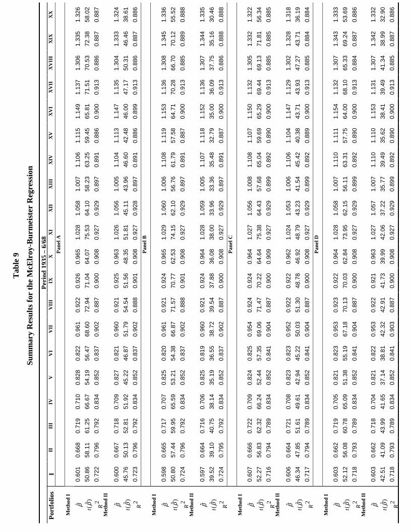
Before approaching the problem of hypothesis testing, Table 9 offers us a very interesting

perspective on the size of the improvement in the degree of precision in parameter

estimation resulting from our procedure. Table 9 in fact shows the beta estimates derived

from the two multi-step regression for the overall sample 1935-196810 and the

corresponding t-statistics. The standard errors for the beta estimates are at least two to

three times smaller than the ones obtained from the simple portfolio grouping procedure

and reported in table 2. Consequently, the t-statistics for our Full-Information MLEs are

two to three times bigger than in the FM results. The reduction in estimation uncertainty

is even more impressive for the gamma parameters, where the standard errors implied by

both Methods 1 and 2 (not reported here but available on request) are generally more than

ten times smaller than their counterparts in Fama-MacBeth11. These results lead to more

precise, although somehow surprising inference in tests for the validation of hypothesis

C1 to C3.

Let’s start with C1, i.e. linearity of the relationship between expected excess return and

beta-measures of risk. Contrary to the early conclusions based on the results of FM

replication, the t-values of table 8 for panels B to D and for Methods 1 and 2 direct us to

reject the null hypothesis. Same is the case when non-beta measures of risk are

considered, as for panels C and D, and t(γ3) is examined. In just two of the 10 subsets of

the data, 1946-1950 and 1956-1960, the evidence supports the assertion that beta is

sufficient to explain a significant portion of the cross-sectional variability of portfolio

returns. Finally, we consider the important null hypothesis C3, i.e. that the expected

excess return-risk trade-off is positive, as argued by any general interpretation of the

Capital Asset Pricing Model. Fortunately again for CAPM lovers, this seems to be the

RN

Z Z Z Z tr VMc i jj

ki i kj j Zk

N

i

2 1

1

1= − − = −

=σ , ( ) ( )( ) ( )Σ , where Vz is the sample covariance

matrix for the portfolio excess returns. 10 The same tables for each of the other nine subsets of the original data are available from the author on

request. 11 As expected, the gain in precision is slightly more significant for Method 1. Nonetheless, Method 2 leads

us to the interesting conclusion that even the estimated Covariance matrix resulting from the pure FM

approach may lead to a huge reduction of estimation uncertainty, when Iterated NLGLS is used.

16

case, for the sample period 1926-1968. Values for t(γ1) are statistically significant, and γ1

positive for most of the subsets considered in the analysis, although still different from

the average excess market returns listed in table 4. In short, we cannot reject the

hypothesis that the pricing of securities listed in the NYSE between 1926 and 1968 is

consistent with the attempts by risk-averse investors to hold efficient portfolios, as

postulated by the CAPM.

5. A Brief Conclusion

The three-step approach devised by Fama and MacBeth survived most of the empirical

results of their paper to become a standard methodology in the financial literature for its

undeniable merits of simplicity and clarity. Nonetheless, their procedure fails to properly

account for estimation errors and lack of independence among cross-sectional residuals.

This uncertainty may lead to false inference, when simple t-statistics are calculated to

empirically validate or disprove hypothesis based on the estimated parameters. In this

paper we proposed a multi-step econometric methodology that attempts to control for the

main drawbacks of the FM technology and mitigates the sensitivity of any analysis of

CAPM implications to the choice of a proxy for the market portfolio.

We applied two versions of the new approach to the same set of data originally employed

by Fama and MacBeth in their analysis of the two-parameter Sharpe-Lintner model.

The new resulting empirical evidence leads us to the conclusion that, although there

seems to be on average a positive trade-off between return and risk over the time frame

1926-1968, nonlinearities and non-beta measures of risk play a very important and

apparently systematic role in explaining the cross-sectional variability of excess returns.

17

Bibliography

Brown S., Weinstein M., A New Approach to Testing Asset Pricing Models: The Bilinear

Paradigm, 1983, Journal of Finance, Vol. XXXVIII, No. 3, pp. 711-743.

Campbell J., Lo A., MacKinlay A., The Econometrics of Financial Markets, 1997,

Princeton University Press.

Fama E., MacBeth J., Risk, Return, and Equilibrium: Empirical Tests, 1973, Journal of

Political Economy, Vol. 81, Issue 3, pp. 607-636.

Kandel S., Stambaugh R., Portfolio Inefficiency and the Cross-Section of Expected

Returns, 1995, Journal of Finance, Vol. 50, pp. 157-184.

Limdep – Version 7.0 – User’s Manual, by William H. Greene, 1998.

McElroy M., Burmeister E., Arbitrage Pricing Theory as a Restricted Nonlinear

Multivariate Regression Model, 1988, Journal of Business & Economic Statistics, Vol. 6,

No. 1, pp. 29-42.

Roll R., A Critique of the Asset Pricing Theory’s Tests: Part I, 1977, Journal of Financial

Economics, Vol. 4, pp. 129-176.

Roll R., Ross S., On the Cross-Sectional Relation between Expected Returns and Betas,

1994, Journal of Finance, Vol. 49, pp. 101-122.

Shanken J., On the Estimation of Beta-Pricing Models, 1992, Review of Financial

Studies, Vol. 5, No. 1, pp. 1-33.

Tab

le 1

Port

folio

For

mat

ion,

Est

imat

ion,

and

Tes

ting

Peri

ods

Perio

ds

1

2 3

4 5

6 7

8 9

Port

folio

For

mat

ion

Peri

od

1926

-192

9 19

27-1

933

1931

-193

7 19

35-1

941

1939

-194

5 19

43-1

949

1947

-195

3 19

51-1

957

1955

-196

1

Initi

al E

stim

atio

n Pe

riod

19

30-1

934

1934

-193

8 19

38-1

942

1942

-194

6 19

46-1

950

1950

-195

4 19

54-1

958

1958

-196

2 19

62-1

966

Test

ing

Peri

od

1935

-193

8 19

39-1

942

1943

-194

6 19

47-1

950

1951

-195

4 19

55-1

958

1959

-196

2 19

63-1

966

1967

-196

8

No.

of s

ecur

ities

ava

ilabl

e 68

0 74

2 76

6 86

7 96

4 10

03

1015

12

81

1405

No.

of s

ecur

ities

mee

ting

data

req

uire

men

ts

390

557

579

672

714

770

814

819

807

Table 2

Sample Statistics for Four Selected Estimation Periods

Statistic I II III IV V VI VII VIII IX XPortfolios for Estimation Period 1934-1938

1,ˆ

−tPβ 0.325 0.619 0.561 0.687 0.843 0.644 0.880 0.955 0.979 0.895

)ˆ( 1, −tPs β 0.024 0.027 0.025 0.028 0.024 0.023 0.037 0.029 0.035 0.025

2),( mP RRr 0.737 0.869 0.864 0.881 0.922 0.898 0.874 0.916 0.900 0.923

)( PRs 0.041 0.071 0.064 0.077 0.093 0.072 0.100 0.106 0.110 0.099

)ˆ(1, itPs ε− 0.074 0.079 0.076 0.089 0.096 0.073 0.116 0.112 0.112 0.094

)ˆ( Ps ε 0.021 0.026 0.024 0.026 0.026 0.023 0.035 0.031 0.035 0.027

)ˆ()ˆ( 1, itPP ss εε −0.287 0.324 0.311 0.298 0.273 0.317 0.306 0.274 0.311 0.292

Portfolios for Estimation Period 1942-1946

1,ˆ

−tPβ 0.462 0.539 0.588 0.595 0.710 0.712 0.776 0.778 0.739 0.854

)ˆ( 1, −tPs β 0.044 0.039 0.043 0.034 0.032 0.033 0.033 0.031 0.037 0.036

2),( mP RRr 0.630 0.741 0.740 0.812 0.866 0.860 0.874 0.887 0.844 0.878

)( PRs 0.035 0.037 0.041 0.040 0.046 0.046 0.050 0.050 0.048 0.055

)ˆ(1, itPs ε− 0.054 0.054 0.063 0.054 0.059 0.063 0.063 0.062 0.059 0.067

)ˆ( Ps ε 0.021 0.019 0.021 0.017 0.017 0.017 0.018 0.017 0.019 0.019

)ˆ()ˆ( 1, itPP ss εε −0.389 0.355 0.330 0.317 0.286 0.274 0.280 0.270 0.322 0.286


1,ˆ

−tPβ 0.418 0.559 0.707 0.737 0.780 0.773 0.887 0.966 0.984 0.959

)ˆ( 1, −tPs β 0.040 0.049 0.048 0.036 0.037 0.040 0.048 0.038 0.034 0.033

2),( mP RRr 0.635 0.666 0.763 0.849 0.856 0.839 0.826 0.887 0.903 0.905

)( PRs 0.019 0.025 0.029 0.029 0.031 0.031 0.035 0.037 0.038 0.037

)ˆ(1, itPs ε− 0.040 0.044 0.046 0.048 0.049 0.050 0.053 0.053 0.058 0.052

)ˆ( Ps ε 0.011 0.014 0.014 0.011 0.012 0.012 0.015 0.013 0.012 0.011

)ˆ()ˆ( 1, itPP ss εε −0.286 0.326 0.307 0.233 0.235 0.245 0.279 0.234 0.202 0.216


1,ˆ

−tPβ 0.636 0.608 0.698 0.751 0.820 0.851 0.939 0.912 0.995 0.927

)ˆ( 1, −tPs β 0.043 0.050 0.041 0.045 0.050 0.032 0.034 0.037 0.042 0.037

2),( mP RRr 0.759 0.693 0.806 0.801 0.798 0.892 0.896 0.881 0.876 0.886

)( PRs 0.031 0.031 0.033 0.036 0.039 0.038 0.042 0.042 0.045 0.042

)ˆ(1, itPs ε− 0.049 0.050 0.055 0.057 0.065 0.058 0.068 0.067 0.069 0.064

)ˆ( Ps ε 0.015 0.017 0.015 0.016 0.018 0.013 0.014 0.014 0.016 0.014

)ˆ()ˆ( 1, itPP ss εε −0.309 0.344 0.266 0.282 0.273 0.218 0.202 0.213 0.232 0.222

Table 2 (Continued)

Sample Statistics for Four Selected Estimation Periods

Statistic XI XII XIII XIV XV XVI XVI XVI XIX XXPortfolios for Estimation Period 1934-1938

1,ˆ

−tPβ 1.029 1.109 1.128 1.114 1.235 1.157 1.312 1.315 1.354 1.408

)ˆ( 1, −tPs β 0.028 0.026 0.033 0.032 0.030 0.028 0.032 0.031 0.042 0.044

2),( mP RRr 0.928 0.936 0.920 0.922 0.935 0.935 0.933 0.936 0.915 0.915

)( PRs 0.114 0.122 0.125 0.123 0.136 0.127 0.144 0.145 0.151 0.157

)ˆ(1, itPs ε− 0.094 0.122 0.134 0.118 0.133 0.112 0.139 0.129 0.135 0.153

)ˆ( Ps ε 0.030 0.031 0.035 0.034 0.035 0.032 0.037 0.037 0.044 0.046

)ˆ()ˆ( 1, itPP ss εε −0.326 0.253 0.262 0.291 0.261 0.289 0.268 0.284 0.325 0.300


1,ˆ

−tPβ 0.963 0.984 0.964 1.007 1.365 1.148 1.337 1.295 1.584 1.634

)ˆ( 1, −tPs β 0.030 0.030 0.036 0.035 0.053 0.033 0.038 0.047 0.068 0.082

2),( mP RRr 0.914 0.919 0.896 0.904 0.887 0.921 0.924 0.899 0.872 0.842

)( PRs 0.060 0.062 0.061 0.063 0.087 0.072 0.083 0.082 0.102 0.107

)ˆ(1, itPs ε− 0.074 0.073 0.075 0.080 0.101 0.088 0.086 0.088 0.113 0.120

)ˆ( Ps ε 0.018 0.018 0.020 0.020 0.029 0.020 0.023 0.026 0.036 0.042

)ˆ()ˆ( 1, itPP ss εε −0.241 0.244 0.265 0.246 0.288 0.227 0.267 0.298 0.321 0.354


1,ˆ

−tPβ 1.080 1.100 1.145 1.170 1.086 1.260 1.200 1.292 1.392 1.523

)ˆ( 1, −tPs β 0.026 0.048 0.034 0.050 0.044 0.043 0.044 0.046 0.061 0.082

2),( mP RRr 0.936 0.870 0.918 0.873 0.881 0.905 0.898 0.901 0.871 0.826

)( PRs 0.040 0.043 0.043 0.045 0.042 0.048 0.046 0.049 0.054 0.061

)ˆ(1, itPs ε− 0.058 0.061 0.060 0.064 0.065 0.062 0.065 0.068 0.072 0.090

)ˆ( Ps ε 0.010 0.015 0.012 0.016 0.014 0.015 0.015 0.015 0.019 0.025

)ˆ()ˆ( 1, itPP ss εε −0.178 0.251 0.207 0.251 0.222 0.237 0.227 0.228 0.269 0.281


1,ˆ

−tPβ 0.973 1.002 1.012 1.049 1.031 1.054 1.069 1.086 1.218 1.356

)ˆ( 1, −tPs β 0.040 0.037 0.035 0.036 0.034 0.042 0.040 0.040 0.048 0.067

2),( mP RRr 0.882 0.897 0.904 0.906 0.910 0.885 0.893 0.895 0.887 0.849

)( PRs 0.044 0.045 0.046 0.047 0.046 0.048 0.048 0.049 0.055 0.064

)ˆ(1, itPs ε− 0.069 0.066 0.065 0.069 0.061 0.068 0.074 0.071 0.069 0.075

)ˆ( Ps ε 0.015 0.015 0.014 0.014 0.014 0.016 0.016 0.016 0.019 0.025

)ˆ()ˆ( 1, itPP ss εε −0.220 0.222 0.218 0.209 0.228 0.239 0.213 0.224 0.269 0.329

Tab

le 3

Sum

mar

y R

esul

ts fo

r th

e R

egre

ssio

n Pti

Pt

Pt

Pt

otP

sR

ηε

γβ

γβ

γγ

ˆ)

ˆ (ˆ

ˆˆ

ˆˆ

ˆ3

22

1+

++

+=

Stat

istic

Peri

od

0γ̂

1γ̂

2γ̂

3γ̂

fR

−0γ̂

)0ˆ (γs

) 1ˆ (γs )

2ˆ (γs

)3ˆ (γs

)

0ˆ (0

fR

−γ

ρ

) 1ˆ (γρ

M

)2ˆ (

0γ

ρ

)3ˆ (

0γ

ρ

)0ˆ (γt

) 1ˆ (γt

)

2ˆ (γt

)3ˆ (γt

)

0ˆ (f

Rt

−γ

2 r

)2

(rs

Pane

l A

1935

-6/1

968

0.00

59

0.00

81

0.00

46

0.03

8 0.

066

0.19

0.

01

3.09

2.

45

2.41

0.

24

0.31

1935

-45

0.00

33

0.01

66

0.00

32

0.05

3 0.

098

0.17

-0

.04

0.72

1.

95

0.69

0.

22

0.30

1946

-55

0.00

88

0.00

26

0.00

79

0.02

6 0.

043

0.08

0.

08

3.79

0.

67

3.39

0.

27

0.34

1956

-6/6

8 0.

0057

0.

0050

0.

0031

0.

030

0.04

3

0.

29

0.16

2.

35

1.43

1.

28

0.24

0.

30

1935

-40

-0.0

011

0.01

44

-0.0

011

0.06

6 0.

119

0.18

-0

.09

-0.1

4 1.

03

-0.1

4 0.

16

0.29

1941

-45

0.00

86

0.01

93

0.00

84

0.03

1 0.

066

0.12

0.

15

2.17

2.

28

2.12

0.

30

0.29

1946

-50

0.00

51

0.00

29

0.00

44

0.03

0 0.

049

0.15

0.

05

1.30

0.

46

1.12

0.

35

0.35

1951

-55

0.01

26

0.00

23

0.01

14

0.01

9 0.

035

-0.1

2 0.

13

5.12

0.

51

4.62

0.

20

0.30

1956

-60

0.01

48

-0.0

058

0.01

28

0.02

0 0.

034

0.15

0.

16

5.64

-1

.31

4.85

0.

16

0.32

1961

-6/6

8 -0

.000

4 0.

0121

-0

.003

3 0.

033

0.04

6

0.

26

0.11

-0

.12

2.48

-0

.95

0.29

0.

29

Pane

l B

1935

-6/1

968

0.00

25

0.01

54

-0.0

036

0.

0012

0.

131

0.27

8 0.

142

-0

.17

-0.2

6 -0

.26

0.

38

1.11

-0

.50

0.

19

0.27

0.

32

1935

-45

0.00

53

0.01

26

0.00

21

0.

0052

0.

218

0.46

1 0.

237

-0

.21

-0.3

0 -0

.29

0.

28

0.31

0.

10

0.

27

0.23

0.

31

1946

-55

-0.0

007

0.02

30

-0.0

100

-0

.001

7 0.

034

0.09

7 0.

041

-0

.02

-0.0

3 -0

.09

-0

.23

2.60

-2

.71

-0

.54

0.31

0.

34

1956

-6/6

8 0.

0026

0.

0117

-0

.003

3

0.00

01

0.05

7 0.

118

0.05

8

0.25

0.

18

0.14

0.56

1.

21

-0.7

1

0.01

0.

28

0.32

1935

-40

-0.0

012

0.01

61

-0.0

011

-0

.001

3 0.

292

0.62

1 0.

316

-0

.22

-0.3

0 -0

.30

-0

.04

0.22

-0

.03

-0

.04

0.17

0.

31

1941

-45

0.01

32

0.00

83

0.00

59

0.

0129

0.

053

0.08

9 0.

068

0.

00

-0.1

5 0.

07

1.

91

0.72

0.

67

1.

88

0.30

0.

31

1946

-50

-0.0

011

0.01

61

-0.0

063

-0

.001

8 0.

037

0.10

5 0.

043

0.

05

0.01

-0

.04

-0

.23

1.19

-1

.13

-0

.37

0.38

0.

35

1951

-55

-0.0

004

0.03

00

-0.0

137

-0

.001

6 0.

032

0.08

9 0.

038

-0

.10

-0.0

9 -0

.17

-0

.10

2.62

-2

.83

-0

.39

0.23

0.

31

1956

-60

0.01

05

0.00

40

-0.0

050

0.

0085

0.

035

0.08

5 0.

040

0.

17

0.03

0.

12

2.

32

0.37

-0

.98

1.

87

0.20

0.

31

1961

-6/6

8 -0

.002

6 0.

0168

-0

.002

2

-0.0

055

0.06

7 0.

135

0.06

7

0.25

0.

22

0.14

-0.3

7 1.

17

-0.3

1

-0.7

8 0.

32

0.32

Tab

le 3

(Con

tinue

d)

Sum

mar

y R

esul

ts fo

r th

e R

egre

ssio

n Pti

Pt

Pt

Pt

otP

sR

ηε

γβ

γβ

γγ

ˆ)

ˆ (ˆ

ˆˆ

ˆˆ

ˆ3

22

1+

++

+=

Stat

istic

Peri

od

0γ̂

1γ̂

2γ̂

3γ̂

fR

−0γ̂

)0ˆ (γs

) 1ˆ (γs )

2ˆ (γs

)3ˆ (γs

)

0ˆ (0

fR

−γ

ρ

) 1ˆ (γρ

M

)2ˆ (

0γ

ρ

)3ˆ (

0γ

ρ

)0ˆ (γt

) 1ˆ (γt

)

2ˆ (γt

)3ˆ (γt

)

0ˆ (f

Rt

−γ

2 r

)2

(rs

Pane

l C

1935

-6/1

968

0.00

63

0.00

88

-0

.013

8 0.

0050

0.

049

0.07

3

0.88

5 0.

10

-0.1

1

0.00

2.

54

2.42

-0.3

1 2.

02

0.26

0.

32

1935

-45

0.00

38

0.01

65

0.

0055

0.

0037

0.

065

0.10

3

0.86

6 0.

07

-0.1

8

-0.0

7 0.

67

1.85

0.07

0.

65

0.25

0.

31

1946

-55

0.01

07

0.00

63

-0

.089

7 0.

0098

0.

038

0.05

8

0.80

9 0.

01

0.03

-0.1

2 3.

11

1.20

-1.2

1 2.

84

0.29

0.

34

1956

-6/6

8 0.

0049

0.

0040

0.03

00

0.00

23

0.04

1 0.

048

0.

959

0.22

0.

00

0.

11

1.46

1.

02

0.

38

0.69

0.

26

0.31

1935

-40

0.00

03

0.01

45

-0

.005

7 0.

0003

0.

071

0.12

8

0.77

3 0.

09

-0.1

6

-0.2

2 0.

04

0.96

-0.0

6 0.

03

0.18

0.

30

1941

-45

0.00

79

0.01

90

0.

0191

0.

0077

0.

058

0.06

0

0.97

3 0.

01

-0.2

9

0.04

1.

07

2.46

0.15

1.

04

0.32

0.

30

1946

-50

0.00

64

0.00

61

-0

.067

3 0.

0058

0.

046

0.07

0

0.86

4 0.

04

0.06

-0.0

2 1.

08

0.68

-0.6

0 0.

96

0.38

0.

35

1951

-55

0.01

50

0.00

66

-0

.112

2 0.

0138

0.

026

0.04

4

0.75

7 -0

.13

-0.0

3

-0.2

6 4.

39

1.16

-1.1

5 4.

03

0.21

0.

30

1956

-60

0.01

25

-0.0

082

0.

0817

0.

0105

0.

033

0.04

5

0.99

1 0.

14

0.02

0.25

2.

90

-1.4

3

0.64

2.

44

0.18

0.

31

1961

-6/6

8 -0

.000

2 0.

0122

-0.0

044

-0.0

031

0.04

5 0.

049

0.

940

0.23

-0

.08

0.

01

-0.0

5 2.

36

-0

.04

-0.6

6 0.

31

0.30

Pane

l D

1935

-6/1

968

0.00

17

0.01

40

-0.0

036

0.03

79

0.00

04

0.14

7 0.

279

0.14

9 0.

918

-0.2

1 -0

.24

-0.2

7 -0

.09

0.23

1.

00

-0.4

8 0.

83

0.06

0.

28

0.33

1935

-45

0.00

66

0.01

15

0.00

27

-0.0

018

0.00

65

0.24

4 0.

459

0.24

9 0.

871

-0.2

5 -0

.28

-0.2

9 -0

.19

0.31

0.

29

0.13

-0

.02

0.31

0.

25

0.32

1946

-55

-0.0

014

0.02

24

-0.0

101

0.01

19

-0.0

024

0.04

5 0.

097

0.04

0 0.

765

-0.0

4 -0

.02

-0.0

8 -0

.12

-0.3

4 2.

52

-2.8

0 0.

17

-0.5

8 0.

31

0.35

1956

-6/6

8 -0

.000

2 0.

0094

-0

.003

9 0.

0935

-0

.002

7 0.

065

0.12

9 0.

062

1.06

2 0.

16

0.06

0.

05

-0.0

2 -0

.03

0.89

-0

.77

1.08

-0

.51

0.29

0.

33

1935

-40

0.00

02

0.01

28

-0.0

002

0.01

71

0.00

01

0.32

4 0.

618

0.33

2 0.

818

-0.2

4 -0

.28

-0.3

0 -0

.21

0.00

0.

18

-0.0

1 0.

18

0.00

0.

19

0.31

1941

-45

0.01

44

0.00

99

0.00

63

-0.0

244

0.01

41

0.07

3 0.

090

0.06

7 0.

937

-0.3

6 -0

.01

-0.0

5 -0

.18

1.52

0.

85

0.72

-0

.20

1.50

0.

32

0.32

1946

-50

-0.0

032

0.01

62

-0.0

075

0.03

69

-0.0

039

0.04

3 0.

106

0.03

7 0.

690

-0.0

6 0.

01

-0.0

8 0.

01

-0.5

7 1.

19

-1.5

6 0.

41

-0.7

0 0.

38

0.37

1951

-55

0.00

03

0.02

86

-0.0

127

-0.0

131

-0.0

009

0.04

7 0.

088

0.04

2 0.

839

-0.0

2 -0

.08

-0.1

0 -0

.20

0.06

2.

51

-2.3

5 -0

.12

-0.1

4 0.

23

0.31

1956

-60

0.00

57

0.00

14

-0.0

064

0.14

86

0.00

37

0.05

5 0.

091

0.04

7 1.

192

-0.1

8 0.

05

-0.1

0 0.

04

0.80

0.

12

-1.0

5 0.

97

0.52

0.

21

0.31

1961

-6/6

8 -0

.004

1 0.

0146

-0

.002

3 0.

0568

-0

.007

0 0.

071

0.14

9 0.

071

0.97

1 0.

29

0.06

0.

09

-0.0

8 -0

.55

0.93

-0

.31

0.55

-0

.93

0.34

0.

33

Table 4

The Behavior of the Market

Statistic

Period m

R fR

mR −

1γ̂

0γ̂

fR

)(m

Rsf

Rm

R −

)(1ˆ

mRs

γ

)(m

Rs )1

ˆ(γs

1935-6/1968 0.0144 0.0131 0.0081 0.0059 0.0046 0.2148 0.1325 0.061 0.066 1935-45 0.0199 0.0197 0.0166 0.0033 0.0032 0.2225 0.1876 0.089 0.098 1946-55 0.0112 0.0103 0.0026 0.0088 0.0079 0.2375 0.0603 0.043 0.043

1956-6/68 0.0121 0.0096 0.0050 0.0057 0.0031 0.2402 0.1245 0.040 0.043 1935-40 0.0137 0.0136 0.0144 -0.0011 -0.0011 0.1260 0.1336 0.108 0.119 1941-45 0.0273 0.0271 0.0193 0.0086 0.0084 0.4702 0.3345 0.058 0.066 1946-50 0.0077 0.0070 0.0029 0.0051 0.0044 0.1350 0.0561 0.052 0.049 1951-55 0.0148 0.0136 0.0023 0.0126 0.0114 0.4163 0.0708 0.033 0.035 1956-60 0.0091 0.0071 -0.0058 0.0148 0.0128 0.2095 -0.1703 0.034 0.034

1961-6/68 0.0141 0.0112 0.0121 -0.0004 -0.0033 0.2583 0.2786 0.043 0.046

Table 4 (Continued)

The Behavior of the Market

Statistic

Period )0

ˆ(γs )(f

Rs )(m

Rt )(f

Rm

Rt − )1ˆ(γt )

0ˆ(γt

)(m

RMρ

)( fRmRM −ρ

)1ˆ(γρ M

)0ˆ(γρ M

)(

fRMρ

1935-6/1968 0.038 0.0012 4.73 4.30 2.45 3.09 -0.01 -0.01 0.01 0.19 0.99

1935-45 0.053 0.0001 2.57 2.56 1.95 0.72 -0.07 -0.07 -0.04 0.17 0.92 1946-55 0.026 0.0004 2.84 2.60 0.67 3.79 0.09 0.09 0.08 0.08 0.95

1956-6/68 0.030 0.0008 3.73 2.94 1.43 2.35 0.14 0.14 0.16 0.28 0.94 1935-40 0.066 0.0001 1.07 1.07 1.03 -0.14 -0.13 -0.13 -0.09 0.18 0.86 1941-45 0.031 0.0001 3.67 3.64 2.28 2.17 0.16 0.16 0.15 0.12 0.93 1946-50 0.030 0.0003 1.15 1.05 0.46 1.30 0.10 0.10 0.05 0.15 0.96 1951-55 0.019 0.0004 3.51 3.21 0.51 5.12 0.05 0.05 0.13 -0.13 0.88 1956-60 0.020 0.0006 2.08 1.61 -1.31 5.64 0.11 0.12 0.16 0.15 0.81

1961-6/68 0.033 0.0007 3.09 2.45 2.48 -0.12 0.14 0.14 0.11 0.26 0.97

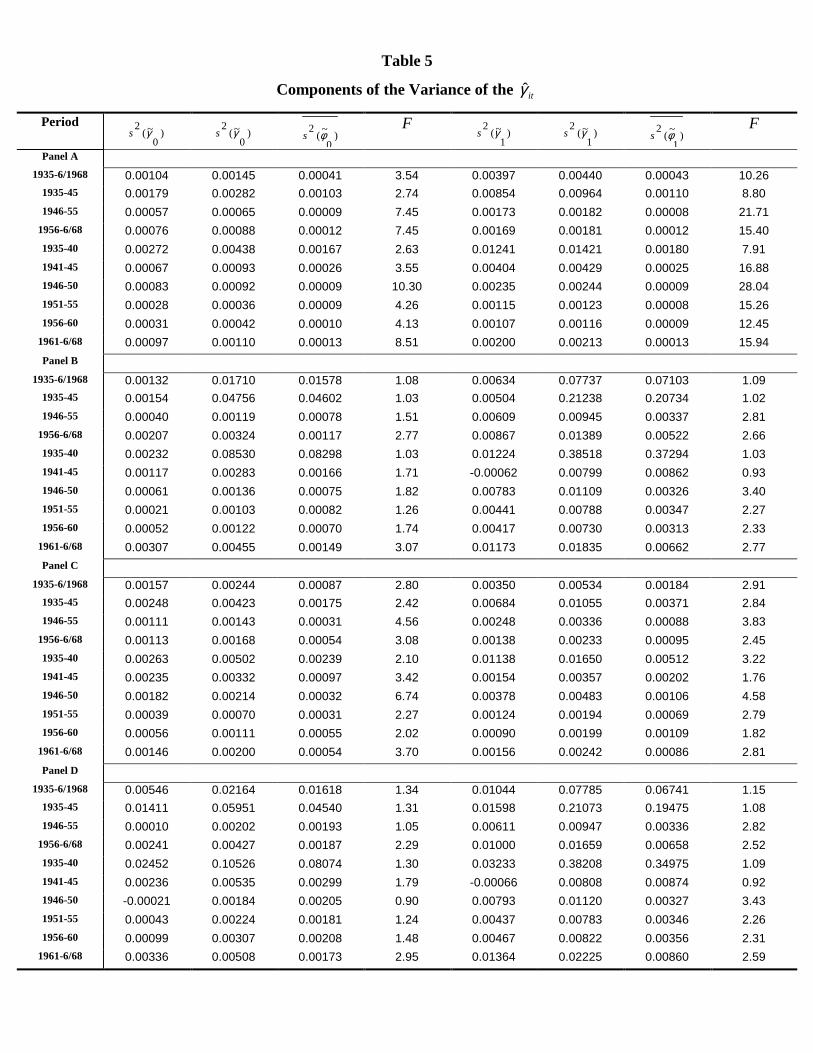
Table 5

Components of the Variance of the itγ̂

Period )

0~(

2 γs )0

~(2 γs )

0~(

2 φs F

)1

~(2 γs )

1~(

2 γs )1

~(2 φs

F

Panel A

1935-6/1968 0.00104 0.00145 0.00041 3.54 0.00397 0.00440 0.00043 10.26 1935-45 0.00179 0.00282 0.00103 2.74 0.00854 0.00964 0.00110 8.80 1946-55 0.00057 0.00065 0.00009 7.45 0.00173 0.00182 0.00008 21.71

1956-6/68 0.00076 0.00088 0.00012 7.45 0.00169 0.00181 0.00012 15.40 1935-40 0.00272 0.00438 0.00167 2.63 0.01241 0.01421 0.00180 7.91 1941-45 0.00067 0.00093 0.00026 3.55 0.00404 0.00429 0.00025 16.88 1946-50 0.00083 0.00092 0.00009 10.30 0.00235 0.00244 0.00009 28.04 1951-55 0.00028 0.00036 0.00009 4.26 0.00115 0.00123 0.00008 15.26 1956-60 0.00031 0.00042 0.00010 4.13 0.00107 0.00116 0.00009 12.45

1961-6/68 0.00097 0.00110 0.00013 8.51 0.00200 0.00213 0.00013 15.94 Panel B

1935-6/1968 0.00132 0.01710 0.01578 1.08 0.00634 0.07737 0.07103 1.09 1935-45 0.00154 0.04756 0.04602 1.03 0.00504 0.21238 0.20734 1.02 1946-55 0.00040 0.00119 0.00078 1.51 0.00609 0.00945 0.00337 2.81

1956-6/68 0.00207 0.00324 0.00117 2.77 0.00867 0.01389 0.00522 2.66 1935-40 0.00232 0.08530 0.08298 1.03 0.01224 0.38518 0.37294 1.03 1941-45 0.00117 0.00283 0.00166 1.71 -0.00062 0.00799 0.00862 0.93 1946-50 0.00061 0.00136 0.00075 1.82 0.00783 0.01109 0.00326 3.40 1951-55 0.00021 0.00103 0.00082 1.26 0.00441 0.00788 0.00347 2.27 1956-60 0.00052 0.00122 0.00070 1.74 0.00417 0.00730 0.00313 2.33

1961-6/68 0.00307 0.00455 0.00149 3.07 0.01173 0.01835 0.00662 2.77 Panel C

1935-6/1968 0.00157 0.00244 0.00087 2.80 0.00350 0.00534 0.00184 2.91 1935-45 0.00248 0.00423 0.00175 2.42 0.00684 0.01055 0.00371 2.84 1946-55 0.00111 0.00143 0.00031 4.56 0.00248 0.00336 0.00088 3.83

1956-6/68 0.00113 0.00168 0.00054 3.08 0.00138 0.00233 0.00095 2.45 1935-40 0.00263 0.00502 0.00239 2.10 0.01138 0.01650 0.00512 3.22 1941-45 0.00235 0.00332 0.00097 3.42 0.00154 0.00357 0.00202 1.76 1946-50 0.00182 0.00214 0.00032 6.74 0.00378 0.00483 0.00106 4.58 1951-55 0.00039 0.00070 0.00031 2.27 0.00124 0.00194 0.00069 2.79 1956-60 0.00056 0.00111 0.00055 2.02 0.00090 0.00199 0.00109 1.82

1961-6/68 0.00146 0.00200 0.00054 3.70 0.00156 0.00242 0.00086 2.81 Panel D

1935-6/1968 0.00546 0.02164 0.01618 1.34 0.01044 0.07785 0.06741 1.15 1935-45 0.01411 0.05951 0.04540 1.31 0.01598 0.21073 0.19475 1.08 1946-55 0.00010 0.00202 0.00193 1.05 0.00611 0.00947 0.00336 2.82

1956-6/68 0.00241 0.00427 0.00187 2.29 0.01000 0.01659 0.00658 2.52 1935-40 0.02452 0.10526 0.08074 1.30 0.03233 0.38208 0.34975 1.09 1941-45 0.00236 0.00535 0.00299 1.79 -0.00066 0.00808 0.00874 0.92 1946-50 -0.00021 0.00184 0.00205 0.90 0.00793 0.01120 0.00327 3.43 1951-55 0.00043 0.00224 0.00181 1.24 0.00437 0.00783 0.00346 2.26 1956-60 0.00099 0.00307 0.00208 1.48 0.00467 0.00822 0.00356 2.31

1961-6/68 0.00336 0.00508 0.00173 2.95 0.01364 0.02225 0.00860 2.59

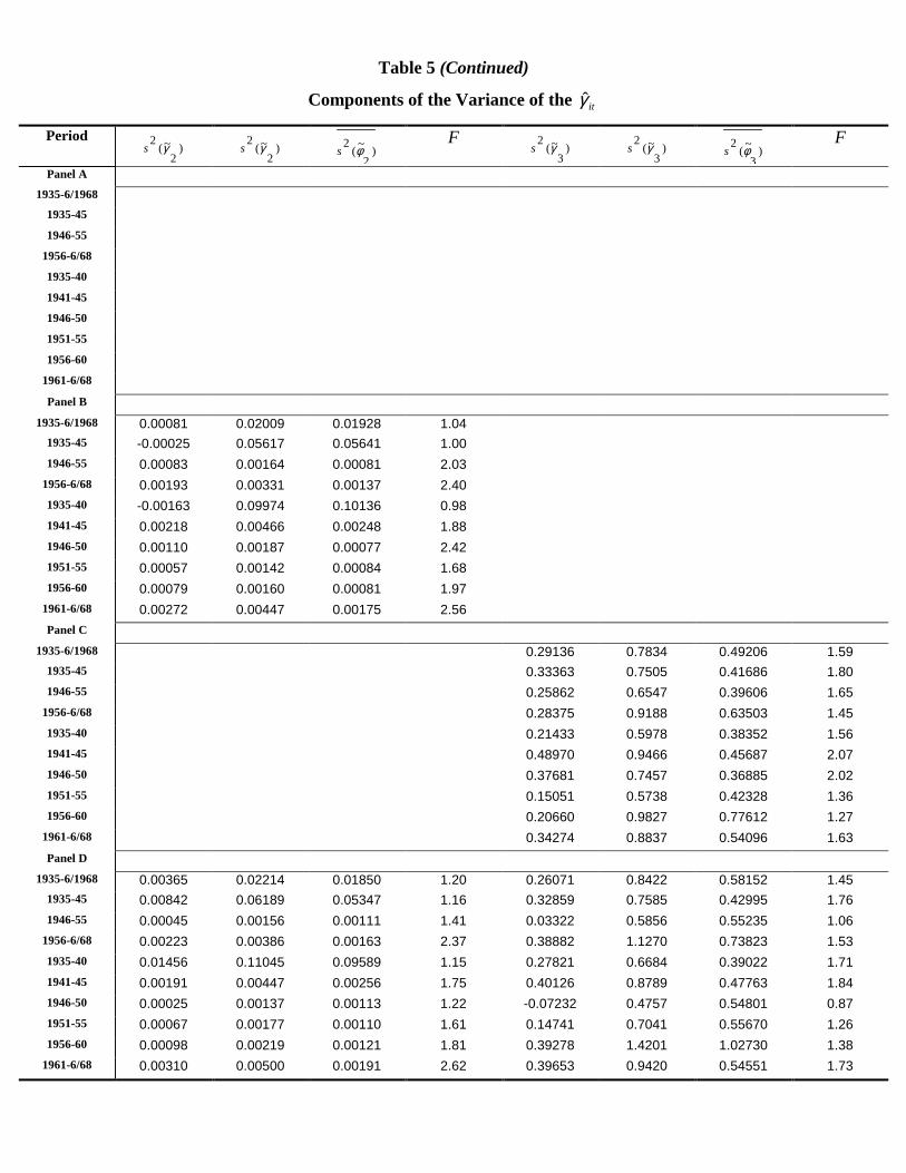
Table 5 (Continued)

Components of the Variance of the itγ̂

Period )

2~(

2 γs )2

~(2 γs )

2~(

2 φs F

)3

~(2 γs )

3~(

2 γs )3

~(2 φs

F

Panel A

1935-6/1968 1935-45 1946-55

1956-6/68 1935-40 1941-45 1946-50 1951-55 1956-60

1961-6/68 Panel B

1935-6/1968 0.00081 0.02009 0.01928 1.04 1935-45 -0.00025 0.05617 0.05641 1.00 1946-55 0.00083 0.00164 0.00081 2.03

1956-6/68 0.00193 0.00331 0.00137 2.40 1935-40 -0.00163 0.09974 0.10136 0.98 1941-45 0.00218 0.00466 0.00248 1.88 1946-50 0.00110 0.00187 0.00077 2.42 1951-55 0.00057 0.00142 0.00084 1.68 1956-60 0.00079 0.00160 0.00081 1.97

1961-6/68 0.00272 0.00447 0.00175 2.56 Panel C

1935-6/1968 0.29136 0.7834 0.49206 1.59 1935-45 0.33363 0.7505 0.41686 1.80 1946-55 0.25862 0.6547 0.39606 1.65

1956-6/68 0.28375 0.9188 0.63503 1.45 1935-40 0.21433 0.5978 0.38352 1.56 1941-45 0.48970 0.9466 0.45687 2.07 1946-50 0.37681 0.7457 0.36885 2.02 1951-55 0.15051 0.5738 0.42328 1.36 1956-60 0.20660 0.9827 0.77612 1.27

1961-6/68 0.34274 0.8837 0.54096 1.63 Panel D

1935-6/1968 0.00365 0.02214 0.01850 1.20 0.26071 0.8422 0.58152 1.45 1935-45 0.00842 0.06189 0.05347 1.16 0.32859 0.7585 0.42995 1.76 1946-55 0.00045 0.00156 0.00111 1.41 0.03322 0.5856 0.55235 1.06

1956-6/68 0.00223 0.00386 0.00163 2.37 0.38882 1.1270 0.73823 1.53 1935-40 0.01456 0.11045 0.09589 1.15 0.27821 0.6684 0.39022 1.71 1941-45 0.00191 0.00447 0.00256 1.75 0.40126 0.8789 0.47763 1.84 1946-50 0.00025 0.00137 0.00113 1.22 -0.07232 0.4757 0.54801 0.87 1951-55 0.00067 0.00177 0.00110 1.61 0.14741 0.7041 0.55670 1.26 1956-60 0.00098 0.00219 0.00121 1.81 0.39278 1.4201 1.02730 1.38

1961-6/68 0.00310 0.00500 0.00191 2.62 0.39653 0.9420 0.54551 1.73

Table 6

Shanken (1992) Adjustment 2))(( ii sc γγ=

Period )(m

Rs )( 0γ̂c )( 1γ̂c )( 2γ̂c )( 3γ̂c )0ˆ( fRc −γ *)0ˆ(γt *)1ˆ(γt *)2ˆ(γt *)3ˆ(γt *)0ˆ( fRt −γ

Panel A

1935-6/1968 0.061 0.009 0.018 0.006 3.07 2.43 2.40 1935-45 0.089 0.001 0.035 0.001 0.72 1.91 0.69 1946-55 0.043 0.042 0.004 0.033 3.72 0.67 3.33

1956-6/68 0.040 0.020 0.015 0.006 2.33 1.42 1.28 1935-40 0.108 0.000 0.018 0.000 -0.14 1.02 -0.14 1941-45 0.058 0.022 0.112 0.021 2.15 2.16 2.10 1946-50 0.052 0.010 0.003 0.007 1.29 0.46 1.12 1951-55 0.033 0.149 0.005 0.122 4.77 0.51 4.36 1956-60 0.034 0.193 0.029 0.144 5.16 -1.29 4.53

1961-6/68 0.043 0.000 0.078 0.006 -0.12 2.39 -0.95 Panel B

1935-6/1968 0.061 0.002 0.063 0.003 0.000 0.38 1.07 -0.50 0.19 1935-45 0.089 0.004 0.020 0.001 0.003 0.28 0.31 0.10 0.27 1946-55 0.043 0.000 0.283 0.054 0.002 -0.23 2.29 -2.64 -0.54

1956-6/68 0.040 0.004 0.086 0.007 0.000 0.56 1.16 -0.71 0.01 1935-40 0.108 0.000 0.022 0.000 0.000 -0.04 0.22 -0.03 -0.04 1941-45 0.058 0.052 0.021 0.010 0.050 1.87 0.71 0.66 1.84 1946-50 0.052 0.000 0.096 0.015 0.001 -0.23 1.13 -1.13 -0.37 1951-55 0.033 0.000 0.846 0.177 0.002 -0.10 1.93 -2.61 -0.39 1956-60 0.034 0.096 0.014 0.022 0.063 2.22 0.36 -0.97 1.81

1961-6/68 0.043 0.004 0.149 0.003 0.016 -0.37 1.10 -0.31 -0.77 Panel C

1935-6/1968 0.061 0.011 0.021 0.05 0.007 2.53 2.40 -0.30 2.01 1935-45 0.089 0.002 0.035 0.00 0.002 0.67 1.82 0.07 0.65 1946-55 0.043 0.061 0.021 4.28 0.051 3.02 1.19 -0.53 2.77

1956-6/68 0.040 0.015 0.010 0.56 0.003 1.45 1.02 0.31 0.69 1935-40 0.108 0.000 0.018 0.00 0.000 0.04 0.95 -0.06 0.03 1941-45 0.058 0.019 0.108 0.10 0.018 1.06 2.34 0.14 1.03 1946-50 0.052 0.015 0.014 1.67 0.012 1.07 0.68 -0.37 0.96 1951-55 0.033 0.212 0.041 11.8 0.179 3.99 1.13 -0.32 3.71 1956-60 0.034 0.137 0.060 5.84 0.096 2.72 -1.39 0.24 2.33

1961-6/68 0.043 0.000 0.079 0.01 0.005 -0.05 2.27 -0.04 -0.66 Panel D

1935-6/1968 0.061 0.001 0.052 0.003 0.38 0.000 0.23 0.98 -0.48 0.70 0.06 1935-45 0.089 0.006 0.017 0.001 0.00 0.005 0.31 0.29 0.13 -0.02 0.30 1946-55 0.043 0.001 0.267 0.054 0.07 0.003 -0.34 2.24 -2.73 0.16 -0.57

1956-6/68 0.040 0.000 0.055 0.010 5.52 0.005 -0.03 0.87 -0.77 0.42 -0.51 1935-40 0.108 0.000 0.014 0.000 0.02 0.000 0.00 0.17 -0.01 0.18 0.00 1941-45 0.058 0.062 0.029 0.012 0.17 0.060 1.48 0.84 0.72 -0.19 1.45 1946-50 0.052 0.004 0.097 0.021 0.50 0.006 -0.57 1.13 -1.55 0.34 -0.70 1951-55 0.033 0.000 0.771 0.153 0.16 0.001 0.06 1.88 -2.19 -0.11 -0.14 1956-60 0.034 0.029 0.002 0.035 19.3 0.012 0.79 0.12 -1.03 0.21 0.52

1961-6/68 0.043 0.009 0.114 0.003 1.71 0.026 -0.54 0.88 -0.30 0.34 -0.92

Table 7

Shanken (1992) & Campbell-Lo-MacKinlay Adjustment

[ ] ftmtmtmm RRZii

−=−+⋅= ˆ)ˆˆ(1' 220

22 σγµσσ γγ

Period )(m

Zs mZ )(γc

)'( 0γ̂s )'( 1γ̂s )'( 2γ̂s )'( 3γ̂s )'0ˆ( fRs −γ )'0ˆ(γt )'1ˆ(γt )'2ˆ(γt )'3ˆ(γt )'0ˆ( fRt −γ

Panel A

1935-6/1968 0.061 0.013 1.014 0.038 0.067 0.038 3.06 2.43 2.39 1935-45 0.089 0.020 1.034 0.054 0.100 0.054 0.71 1.91 0.68

1946-55 0.043 0.010 1.001 0.026 0.043 0.026 3.79 0.67 3.39

1956-6/68 0.040 0.010 1.009 0.030 0.043 0.030 2.34 1.42 1.28

1935-40 0.108 0.014 1.018 0.067 0.120 0.067 -0.13 1.02 -0.14

1941-45 0.058 0.027 1.103 0.032 0.069 0.032 2.07 2.17 2.02

1946-50 0.052 0.007 1.001 0.030 0.049 0.030 1.30 0.46 1.12

1951-55 0.033 0.014 1.001 0.019 0.035 0.019 5.12 0.51 4.61

1956-60 0.034 0.007 1.052 0.021 0.035 0.021 5.50 -1.27 4.73

1961-6/68 0.043 0.011 1.072 0.034 0.048 0.034 -0.11 2.40 -0.92

Panel B

1935-6/1968 0.061 0.013 1.030 0.133 0.282 0.144 0.133 0.38 1.09 -0.50 0.18 1935-45 0.089 0.020 1.026 0.221 0.467 0.240 0.221 0.28 0.31 0.10 0.27

1946-55 0.043 0.010 1.065 0.036 0.100 0.042 0.036 -0.23 2.52 -2.63 -0.52

1956-6/68 0.040 0.010 1.030 0.058 0.120 0.058 0.058 0.56 1.20 -0.70 0.01

1935-40 0.108 0.014 1.019 0.295 0.626 0.319 0.295 -0.04 0.22 -0.03 -0.04

1941-45 0.058 0.027 1.059 0.055 0.092 0.070 0.055 1.86 0.70 0.65 1.83

1946-50 0.052 0.007 1.024 0.037 0.107 0.044 0.037 -0.22 1.17 -1.12 -0.37

1951-55 0.033 0.014 1.182 0.035 0.097 0.041 0.035 -0.09 2.41 -2.60 -0.36

1956-60 0.034 0.007 1.010 0.035 0.086 0.040 0.035 2.31 0.37 -0.97 1.86

1961-6/68 0.043 0.011 1.102 0.071 0.142 0.070 0.071 -0.35 1.12 -0.30 -0.74

Panel C

1935-6/1968 0.061 0.013 1.013 0.050 0.074 0.891 0.050 2.53 2.41 -0.31 2.01 1935-45 0.089 0.020 1.032 0.066 0.104 0.880 0.066 0.66 1.82 0.07 0.64

1946-55 0.043 0.010 1.000 0.038 0.058 0.809 0.038 3.11 1.20 -1.21 2.84

1956-6/68 0.040 0.010 1.014 0.041 0.049 0.965 0.041 1.45 1.02 0.38 0.69

1935-40 0.108 0.014 1.015 0.071 0.129 0.779 0.071 0.04 0.95 -0.06 0.03

1941-45 0.058 0.027 1.111 0.061 0.063 1.025 0.061 1.01 2.33 0.14 0.98

1946-50 0.052 0.007 1.000 0.046 0.070 0.864 0.046 1.08 0.68 -0.60 0.96

1951-55 0.033 0.014 1.002 0.026 0.044 0.758 0.027 4.39 1.15 -1.15 4.03

1956-60 0.034 0.007 1.025 0.034 0.045 1.004 0.034 2.87 -1.41 0.63 2.40

1961-6/68 0.043 0.011 1.069 0.046 0.051 0.972 0.046 -0.04 2.28 -0.04 -0.64

Panel D

1935-6/1968 0.061 0.013 1.035 0.150 0.284 0.151 0.934 0.150 0.23 0.99 -0.47 0.81 0.05 1935-45 0.089 0.020 1.022 0.247 0.464 0.251 0.880 0.247 0.31 0.28 0.12 -0.02 0.30

1946-55 0.043 0.010 1.073 0.047 0.101 0.041 0.793 0.047 -0.33 2.44 -2.70 0.16 -0.56

1956-6/68 0.040 0.010 1.060 0.067 0.133 0.064 1.093 0.067 -0.03 0.86 -0.75 1.05 -0.49

1935-40 0.108 0.014 1.016 0.327 0.623 0.335 0.824 0.327 0.00 0.17 -0.01 0.18 0.00

1941-45 0.058 0.027 1.049 0.075 0.092 0.068 0.960 0.075 1.48 0.83 0.71 -0.20 1.46

1946-50 0.052 0.007 1.038 0.044 0.108 0.038 0.703 0.044 -0.56 1.16 -1.53 0.41 -0.68

1951-55 0.033 0.014 1.163 0.051 0.095 0.045 0.905 0.051 0.05 2.32 -2.18 -0.11 -0.13

1956-60 0.034 0.007 1.002 0.055 0.091 0.047 1.193 0.055 0.80 0.12 -1.05 0.97 0.52

1961-6/68 0.043 0.011 1.125 0.076 0.158 0.075 1.029 0.076 -0.51 0.88 -0.29 0.52 -0.88

Table 8

McElroy-Burmeister Approach to Gamma Estimation

1γ̂ 2γ̂ 3γ̂ )ˆ( 1γt

)ˆ( 2γt

)ˆ( 3γt 2

s McElroy'

R 1γ̂ 2γ̂ 3γ̂ )ˆ( 1γt

)ˆ( 2γt

)ˆ( 3γt 2

s McElroy'

R

Period METHOD 1 METHOD 2

Panel A

1935-6/1968 -0.0017 -1.92 0.6323 -0.0012 -0.81 0.4816 1935-45 -0.0009 -2.04 0.9521 0.0003 0.07 0.5829

1946-55 -0.0010 -5.43 0.9653 -0.0004 -0.55 0.8759

1956-6/68 -0.0024 -1.22 0.2661 -0.0008 -0.37 0.1961

1935-40 -0.0010 -1.43 0.9592 0.0012 0.24 0.7192

1941-45 -0.0012 -3.29 0.9727 0.0021 0.41 0.3636

1946-50 -0.0005 -1.92 0.9789 0.0005 0.61 0.9214

1951-55 -0.0013 -5.38 0.9642 0.0001 0.11 0.8760

1956-60 -0.0021 -6.80 0.9552 -0.0035 -4.41 0.8304

1961-6/68 -0.0035 -1.43 0.2674 -0.0006 -0.14 0.1224

Panel B

1935-6/1968 0.0044 -0.0060 1.79 -2.64 0.6326 0.0047 -0.0059 1.61 -2.54 0.3920 1935-45 0.0055 -0.0060 1.02 -1.21 0.9522 0.0064 -0.0060 1.09 -1.13 0.6368

1946-55 0.0064 -0.0069 1.90 -2.20 0.9658 0.0077 -0.0060 1.25 -1.42 0.3851

1956-6/68 0.0012 -0.0038 0.28 -1.00 0.2660 0.0026 -0.0033 0.57 -0.81 0.1589

1935-40 0.0012 -0.0021 0.14 -0.27 0.9593 0.0039 -0.0026 0.38 -0.33 0.7057

1941-45 0.0051 -0.0055 1.20 -1.46 0.9739 0.0049 -0.0034 1.11 -0.66 0.5349

1946-50 -0.0007 0.0002 -0.14 0.04 0.9791 0.0014 0.0010 0.18 0.17 0.6791

1951-55 0.0089 -0.0095 3.41 -3.84 0.9711 0.0131 -0.0103 1.13 -1.12 0.1869

1956-60 0.0119 -0.0130 3.23 -3.76 0.9616 0.0085 -0.0096 2.28 -2.73 0.9600

1961-6/68 -0.0093 0.0070 -1.77 1.12 0.2677 -0.0044 0.0053 -0.62 0.76 0.0985

Panel C

1935-6/1968 -0.0019 -0.0893 -2.03 -11.00 0.6311 -0.0013 -0.0941 -0.80 -10.47 0.4645 1935-45 -0.0010 -0.1177 -2.17 -5.23 0.9518 0.0002 -0.1097 0.05 -4.88 0.5858

1946-55 -0.0011 -0.0566 -5.69 -2.39 0.9653 0.0006 -0.0763 0.44 -3.08 0.6985

1956-6/68 -0.0024 -0.0492 -1.22 -2.64 0.2642 -0.0010 -0.0501 -0.46 -2.60 0.2038

1935-40 -0.0010 -0.1283 -1.45 -3.46 0.9586 0.0012 -0.1074 0.24 -3.00 0.7197

1941-45 -0.0013 -0.1085 -3.53 -2.23 0.9726 0.0022 -0.0861 0.42 -1.90 0.3676

1946-50 -0.0005 -0.0367 -1.95 -0.86 0.9788 0.0017 -0.0644 1.14 -1.39 0.8141

1951-55 -0.0014 -0.0749 -5.36 -1.49 0.9624 0.0019 -0.1061 1.47 -2.22 0.6450

1956-60 -0.0021 0.0007 -6.24 0.02 0.9565 -0.0045 -0.0036 -3.14 -0.09 0.6515

1961-6/68 -0.0037 -0.0657 -1.48 -2.53 0.2668 -0.0005 -0.0686 -0.13 -2.61 0.1216

Panel D

1935-6/1968 0.0047 -0.0064 -0.0900 1.89 -2.80 -11.02 0.6314 0.0050 -0.0064 -0.0903 1.75 -2.74 -9.77 0.4247 1935-45 0.0060 -0.0065 -0.1184 1.08 -1.28 -5.27 0.9519 0.0067 -0.0065 -0.1119 1.13 -1.21 -4.98 0.6488

1946-55 0.0069 -0.0074 -0.0599 2.04 -2.36 -2.52 0.9658 0.0080 -0.0064 -0.0587 1.30 -1.51 -2.35 0.4115

1956-6/68 0.0011 -0.0038 -0.0490 0.26 -1.00 -2.62 0.2642 0.0023 -0.0036 -0.0410 0.52 -0.91 -2.12 0.1821

1935-40 0.0001 -0.0011 -0.1282 0.01 -0.13 -3.46 0.9587 0.0029 -0.0020 -0.1007 0.29 -0.25 -2.81 0.7590

1941-45 0.0059 -0.0063 -0.1162 1.41 -1.69 -2.39 0.9739 0.0057 -0.0038 -0.1036 1.25 -0.67 -2.27 0.4787

1946-50 -0.0008 0.0003 -0.0374 -0.16 0.06 -0.85 0.9790 0.0014 0.0006 -0.0270 0.18 0.10 -0.58 0.7275

1951-55 0.0097 -0.0103 -0.0924 3.84 -4.28 -1.75 0.9692 0.0139 -0.0109 -0.0825 1.20 -1.17 -1.62 0.1943

1956-60 0.0122 -0.0133 -0.0262 3.28 -3.83 -0.59 0.9618 0.0090 -0.0111 0.0091 1.94 -2.83 0.21 0.7997

1961-6/68 -0.0103 0.0080 -0.0678 -1.88 1.22 -2.53 0.2672 -0.0058 0.0063 -0.0570 -0.82 0.87 -2.10 0.1110

Tab

le 9

Sum

mar

y R

esul

ts fo

r th

e M

cElr

oy-B

urm

eist

er R

egre

ssio

n

Peri

od19

35–

6/68

Port

folio

s I

II

III

IV

V

VI

VII

V

III

IX

X

XI

XII

X

III

XIV

X

V

XV

I X

VII

X

VII

I X

IX

XX

Pane

l A

Met

hod

I

β̂

0.60

1 0.

668

0.71

9 0.

710

0.82

8 0.

822

0.96

1 0.

922

0.92

6 0.

965

1.02

8 1.

058

1.00

7 1.

106

1.11

5 1.

149

1.13

7 1.

306

1.33

5 1.

326

)ˆ(βt

50

.86

58.1

1 61

.25

66.6

7 54

.19

56.4

7 68

.60

72.9

4 71

.04

64.0

7 75

.53

64.1

0 58

.23

63.2

5 59

.45

65.8

1 71

.51

70.5

3 72

.38

58.0

2 2

R

0.72

2 0.

796

0.79

2 0.

834

0.85

2 0.

837

0.90

2 0.

887

0.90

0 0.

908

0.92

7 0.

929

0.89

7 0.

891

0.88

6 0.

900

0.91

3 0.

886

0.88

7 0.

887

Met

hod

II

β̂

0.60

0 0.

667

0.71

8 0.

709

0.82

7 0.

821

0.96

0 0.

921

0.92

5 0.

963

1.02

6 1.

056

1.00

5 1.

104

1.11

3 1.

147

1.13

5 1.

304

1.33

3 1.

324

)ˆ(βt

45

.76

50.1

3 52

.81

51.9

2 45

.22

46.8

7 51

.79

54.5

4 51

.56

48.3

5 51

.81

45.1

1 43

.96

46.6

0 42

.48

46.0

0 47

.17

50.3

1 46

.46

38.6

1 2

R

0.72

3 0.

796

0.79

2 0.

834

0.85

2 0.

837

0.90

2 0.

888

0.90

1 0.

908

0.92

7 0.

928

0.89

7 0.

891

0.88

6 0.

899

0.91

3 0.

886

0.88

7 0.

886

Pa

nel B

Met

hod

I

β̂

0.59

8 0.

665

0.71

7 0.

707

0.82

5 0.

820

0.96

1 0.

921

0.92

4 0.

965

1.02

9 1.

060

1.00

6 1.

108

1.11

9 1.

153

1.13

6 1.

308

1.34

5 1.

336

)ˆ(βt

50

.80

57.4

4 59

.95

65.5

9 53

.21

54.3

8 66

.87

71.5

7 70

.77

62.5

3 74

.15

62.1

0 56

.76

61.7

9 57

.58

64.7

1 70

.28

66.7

0 70

.12

55.5

2 2

R

0.72

4 0.

796

0.79

2 0.

834

0.85

2 0.

837

0.90

2 0.

888

0.90

1 0.

908

0.92

7 0.

929

0.89

7 0.

891

0.88

7 0.

900

0.91

3 0.

885

0.88

9 0.

888

Met

hod

II

β̂

0.59

7 0.

664

0.71

6 0.

706

0.82

5 0.

819

0.96

0 0.

921

0.92

4 0.

964

1.02

8 1.

059

1.00

5 1.

107

1.11

8 1.

152

1.13

6 1.

307

1.34

4 1.

335

)ˆ(βt

39

.52

39.1

0 40

.75

38.1

4 35

.19

36.5

5 38

.72

39.5

4 37

.88

36.0

8 38

.00

33.9

6 33

.36

35.4

8 32

.79

35.0

0 36

.09

37.7

5 35

.16

30.4

6 2

R

0.72

4 0.

795

0.79

2 0.

834

0.85

2 0.

837

0.90

2 0.

887

0.90

0 0.

908

0.92

7 0.

929

0.89

7 0.

891

0.88

7 0.

900

0.91

3 0.

886

0.88

8 0.

888

Pa

nel C

Met

hod

I

β̂

0.60

7 0.

666

0.72

2 0.

709

0.82

4 0.

825

0.95

4 0.

924

0.92

4 0.

964

1.02

7 1.

056

1.00

8 1.

108

1.10

7 1.

150

1.13

2 1.

305

1.33

2 1.

322

)ˆ(βt

52

.27

56.8

3 62

.32

66.2

4 52

.44

57.3

5 69

.06

71.4

7 70

.22

64.6

4 75

.38

64.4

3 57

.68

65.0

4 59

.69

65.2

9 69

.44

69.1

3 71

.81

56.3

4 2

R

0.71

6 0.

794

0.78

9 0.

834

0.85

2 0.

841

0.90

4 0.

887

0.90

0 0.

909

0.92

7 0.

929

0.89

9 0.

892

0.89

0 0.

900

0.91

3 0.

885

0.88

5 0.

885

Met

hod

II

β̂

0.60

6 0.

664

0.72

1 0.

708

0.82

3 0.

823

0.95

2 0.

922

0.92

2 0.

962

1.02

4 1.

053

1.00

6 1.

106

1.10

4 1.

147

1.12

9 1.

302

1.32

8 1.

318

)ˆ(βt

46

.34

47.8

5 51

.61

49.6

1 42

.94

45.2

2 50

.03

51.3

0 48

.78

46.9

2 48

.79

43.2

3 41

.54

45.4

2 40

.38

43.7

1 43

.93

47.2

7 43

.71

36.1

9 2

R

0.71

7 0.

794

0.78

9 0.

834

0.85

2 0.

841

0.90

4 0.

887

0.90

0 0.

908

0.92

7 0.

929

0.89

9 0.

892

0.88

9 0.

900

0.91

3 0.

885

0.88

4 0.

884

Pa

nel D

Met

hod

I

β̂

0.60

3 0.

662

0.71

9 0.

705

0.82

1 0.

823

0.95

3 0.

923

0.92

2 0.

964

1.02

8 1.

058

1.00

7 1.

110

1.11

1 1.

154

1.13

2 1.

307

1.34

3 1.

333

)ˆ(βt

52

.12

56.0

8 60

.78

65.0

9 51

.38

55.1

9 67

.18

70.1

3 70

.03

62.8

4 73

.95

62.1

5 56

.11

63.3

1 57

.75

64.0

0 68

.10

65.3

3 69

.24

53.6

9 2

R

0.71

8 0.

793

0.78

9 0.

834

0.85

2 0.

841

0.90

4 0.

887

0.90

0 0.

908

0.92

7 0.

929

0.89

9 0.

892

0.89

0 0.

900

0.91

3 0.

884

0.88

7 0.

886

Met

hod

II

β̂

0.60

3 0.

662

0.71

8 0.

704

0.82

1 0.

822

0.95

3 0.

922

0.92

1 0.

963

1.02

7 1.

057

1.00

7 1.

110

1.11

0 1.

153

1.13

1 1.

307

1.34

2 1.

332

)ˆ(βt

42

.51

41.0

9 43

.99

41.6

5 37

.14

38.8

1 42

.32

42.9

1 41

.73

39.9

9 42

.06

37.2

2 35

.77

39.4

9 35

.62

38.4

1 39

.49

41.3

4 38

.99

32.9

0 2

R

0.71

8 0.

793

0.78

9 0.

834

0.85

2 0.

841

0.90

3 0.

887

0.90

0 0.

908

0.92

7 0.

929

0.89

9 0.

892

0.89

0 0.

900

0.91

3 0.

885

0.88

7 0.

886

************************************************************************ * PROGRAM: access.f - Sample program to read crsp daily and monthly stock * files using random access programming * * DESCRIPTION: This program takes CRSP perm numbers from a user-created file * called perms.dat. Retrieved information for each security * found is written to an output file called outperm.dat. * * Perm numbers should be entered one to a line in the file * perms.dat in columns 1-5. * * All securities with data in the monthly and daily databases * are listed in the files: * * /dbases/crsp/doc/monthly-stock.listing * /dbases/crsp/doc/daily-stock.listing * * These files can be used to locate perm numbers from the ticker

symbol or the name of a security. * To search the files use the Unix "grep" command. * For example: * * grep FORD /dbases/crsp/doc/monthly-stock.listing | more * * This will print to the screen all companies with "FORD" * in their name. * * USAGE: Change udopen to umopen and udclose to umclose for monthly * data where specified. * * Add code for desired extraction or processing where * specified. See the "Stock File User's Guide" and "Stock * File Programmer's Guide" for assistance. These are * available as Microsoft Word documents in the /dbases/crsp/doc * directory. * * Then, compile the program as follows: f77crsp access.f * * Then run the executable "a.out" generated from the compile * step by simply typing: a.out * ***********************************************************************

program access1 include '/dbases/crsp/include/us.txt' integer kperm open (unit=10,file='perms53.dat',status='old') open (unit=11,file='outperm.dat',status='unknown') c----------------------------------------------------------------------------- call umopen(nyseamex) call umcal(nyse) 100 read (10,1000,end=900) kperm 1000 format(i5) call usgetper(1,kperm,infos+returns,*900) if (kperm. ne . permno) goto 100 call usgetper(1,permno,infos+returns,*900) c ********************************************* c *** *** c *** Insert your processing code here *** c *** *** c *** For example, the following do loop *** c *** writes the cusip, calendar date and *** c *** price for each date that the security *** c *** has price data in the database. *** c ********************************************* do j=350,541 write(11,9001) permno,caldt(j),ret(j),ewretd(j) end do 9001 format (i5,x,i8,x,f11.6,x,f11.6) c ********************************************* c *** End of user inserted code *** c *********************************************

goto 100 ! get another perm number c----------------------------------------------------------------------------- 900 call umclose c----------------------------------------------------------------------------- close(unit=10) close(unit=11) stop end

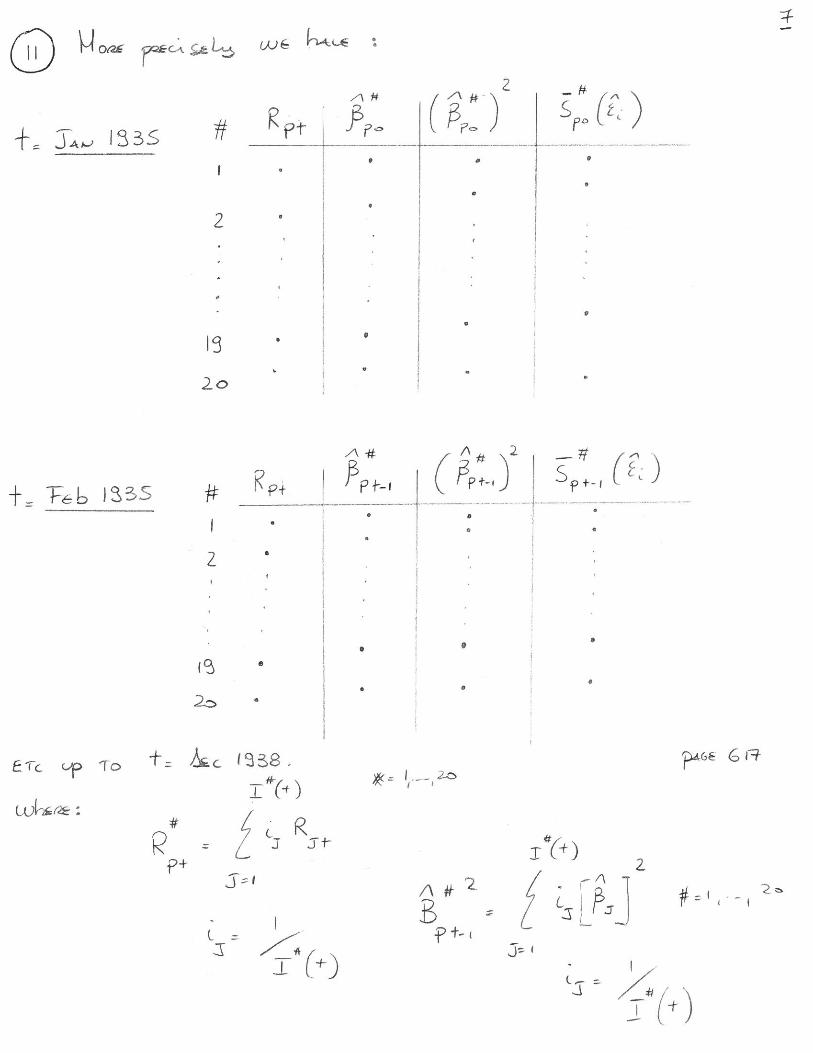
LatestBrownA.lim Page 1

FIRST TRY: FAMA-McBeth is used for the initial values of NLOLS. Then a ITNLGLS is performed-------------------------------------------------------------------------------------------PANEL A ********************************************************************

ok!!!!

calc;T=90;NCF=21;FROM=313;TO=402$read;Nobs=1000;Nvar=22;file=a:/panelA35-68.wks;format=wks$samp;1-NCF$matr;BEGIN=x31$samp;FROM-TO$NLSUR;Lhs=x1,x2,x3,x4,x5,x6,x7,x8,x9,x10,x11,x12,x13,x14,x15,x16,x17,x18,x19,x20 ;start=BEGIN ;Labels=gamma1,20_beta ;Fn1=beta1*(gamma1+x21) ;Fn2=beta2*(gamma1+x21) ;Fn3=beta3*(gamma1+x21) ;Fn4=beta4*(gamma1+x21) ;Fn5=beta5*(gamma1+x21) ;Fn6=beta6*(gamma1+x21) ;Fn7=beta7*(gamma1+x21) ;Fn8=beta8*(gamma1+x21) ;Fn9=beta9*(gamma1+x21) ;Fn10=beta10*(gamma1+x21) ;Fn11=beta11*(gamma1+x21) ;Fn12=beta12*(gamma1+x21) ;Fn13=beta13*(gamma1+x21) ;Fn14=beta14*(gamma1+x21) ;Fn15=beta15*(gamma1+x21) ;Fn16=beta16*(gamma1+x21) ;Fn17=beta17*(gamma1+x21) ;Fn18=beta18*(gamma1+x21) ;Fn19=beta19*(gamma1+x21) ;Fn20=beta20*(gamma1+x21) ;SIGMA=I$matr;EX=[B(1)]+x21$matr;E1=Init(T,1,0);E1=x1-EX*B(2)$matr;E2=Init(T,1,0);E2=x2-EX*B(3)$matr;E3=Init(T,1,0);E3=x3-EX*B(4)$matr;E4=Init(T,1,0);E4=x4-EX*B(5)$matr;E5=Init(T,1,0);E5=x5-EX*B(6)$matr;E6=Init(T,1,0);E6=x6-EX*B(7)$matr;E7=Init(T,1,0);E7=x7-EX*B(8)$matr;E8=Init(T,1,0);E8=x8-EX*B(9)$matr;E9=Init(T,1,0);E9=x9-EX*B(10)$matr;E10=Init(T,1,0);E10=x10-EX*B(11)$matr;E11=Init(T,1,0);E11=x11-EX*B(12)$matr;E12=Init(T,1,0);E12=x12-EX*B(13)$matr;E13=Init(T,1,0);E13=x13-EX*B(14)$matr;E14=Init(T,1,0);E14=x14-EX*B(15)$matr;E15=Init(T,1,0);E15=x15-EX*B(16)$matr;E16=Init(T,1,0);E16=x16-EX*B(17)$matr;E17=Init(T,1,0);E17=x17-EX*B(18)$matr;E18=Init(T,1,0);E18=x18-EX*B(19)$matr;E19=Init(T,1,0);E19=x19-EX*B(20)$matr;E20=Init(T,1,0);E20=x20-EX*B(21)$matr;BIGE1=[E1,E2,E3,E4,E5,E6,E7,E8,E9,E10]$matr;BIGE2=[E11,E12,E13,E14,E15,E16,E17,E18,E19,E20]$matr;BIGE=[BIGE1,BIGE2]$matr;SIGMA1=BIGE'BIGE*<T>$


samp;1-NCF$matr;BEGIN2=B$samp;FROM-TO$NLSUR;Lhs=x1,x2,x3,x4,x5,x6,x7,x8,x9,x10,x11,x12,x13,x14,x15,x16,x17,x18,x19,x20 ;start=BEGIN2 ;Labels=gamma1,20_beta ;Fn1=beta1*(gamma1+x21) ;Fn2=beta2*(gamma1+x21) ;Fn3=beta3*(gamma1+x21) ;Fn4=beta4*(gamma1+x21) ;Fn5=beta5*(gamma1+x21) ;Fn6=beta6*(gamma1+x21) ;Fn7=beta7*(gamma1+x21) ;Fn8=beta8*(gamma1+x21) ;Fn9=beta9*(gamma1+x21) ;Fn10=beta10*(gamma1+x21) ;Fn11=beta11*(gamma1+x21) ;Fn12=beta12*(gamma1+x21) ;Fn13=beta13*(gamma1+x21) ;Fn14=beta14*(gamma1+x21) ;Fn15=beta15*(gamma1+x21) ;Fn16=beta16*(gamma1+x21) ;Fn17=beta17*(gamma1+x21) ;Fn18=beta18*(gamma1+x21) ;Fn19=beta19*(gamma1+x21) ;Fn20=beta20*(gamma1+x21) ;SIGMA=SIGMA1$crea;Paolo=B$matr;VARI=[VARB(1,1)/VARB(2,2)/VARB(3,3)/VARB(4,4)/VARB(5,5)/VARB(6,6)/VARB(7,7)/VARB(8,8)/VARB(9,9)/VARB(10,10)]$matr;VARII=[VARB(11,11)/VARB(12,12)/VARB(13,13)/VARB(14,14)/VARB(15,15)/VARB(16,16)/VARB(17,17)/VARB(18,18)/VARB(19,19)/VARB(20,20)]$matr;VARIII=[VARB(21,21)]$matr;VARIV=[VARI/VARII/VARIII]$crea;Pasqua=VARIV$writ;Paolo,Pasqua;File=a:\outputA61-68.wks;format=wks$

************************************************************************METHOD II

calc;T=90;NCF=21;FROM=313;TO=402$read;Nobs=1000;Nvar=31;file=a:/panelA35-68.wks;format=wks$samp;1-NCF$matr;B1=x31$samp;FROM-TO$matr;EX=[B1(1)]+x21$matr;E1=Init(T,1,0);E1=x1-EX*B1(2)$matr;E2=Init(T,1,0);E2=x2-EX*B1(3)$matr;E3=Init(T,1,0);E3=x3-EX*B1(4)$matr;E4=Init(T,1,0);E4=x4-EX*B1(5)$matr;E5=Init(T,1,0);E5=x5-EX*B1(6)$matr;E6=Init(T,1,0);E6=x6-EX*B1(7)$matr;E7=Init(T,1,0);E7=x7-EX*B1(8)$matr;E8=Init(T,1,0);E8=x8-EX*B1(9)$matr;E9=Init(T,1,0);E9=x9-EX*B1(10)$matr;E10=Init(T,1,0);E10=x10-EX*B1(11)$matr;E11=Init(T,1,0);E11=x11-EX*B1(12)$


matr;E12=Init(T,1,0);E12=x12-EX*B1(13)$matr;E13=Init(T,1,0);E13=x13-EX*B1(14)$matr;E14=Init(T,1,0);E14=x14-EX*B1(15)$matr;E15=Init(T,1,0);E15=x15-EX*B1(16)$matr;E16=Init(T,1,0);E16=x16-EX*B1(17)$matr;E17=Init(T,1,0);E17=x17-EX*B1(18)$matr;E18=Init(T,1,0);E18=x18-EX*B1(19)$matr;E19=Init(T,1,0);E19=x19-EX*B1(20)$matr;E20=Init(T,1,0);E20=x20-EX*B1(21)$matr;BIGEI=[E1,E2,E3,E4,E5,E6,E7,E8,E9,E10];BIGEII=[E11,E12,E13,E14,E15,E16,E17,E18,E19,E20];BIGE=[BIGEI,BIGEII];SIGMA1=BIGE'BIGE*<T>$matr;BEGIN2=B1$samp;FROM-TO$NLSUR;Lhs=x1,x2,x3,x4,x5,x6,x7,x8,x9,x10,x11,x12,x13,x14,x15,x16,x17,x18,x19,x20 ;start=BEGIN2 ;Labels=gamma1,20_beta ;Fn1=beta1*(gamma1+x21) ;Fn2=beta2*(gamma1+x21) ;Fn3=beta3*(gamma1+x21) ;Fn4=beta4*(gamma1+x21) ;Fn5=beta5*(gamma1+x21) ;Fn6=beta6*(gamma1+x21) ;Fn7=beta7*(gamma1+x21) ;Fn8=beta8*(gamma1+x21) ;Fn9=beta9*(gamma1+x21) ;Fn10=beta10*(gamma1+x21) ;Fn11=beta11*(gamma1+x21) ;Fn12=beta12*(gamma1+x21) ;Fn13=beta13*(gamma1+x21) ;Fn14=beta14*(gamma1+x21) ;Fn15=beta15*(gamma1+x21) ;Fn16=beta16*(gamma1+x21) ;Fn17=beta17*(gamma1+x21) ;Fn18=beta18*(gamma1+x21) ;Fn19=beta19*(gamma1+x21) ;Fn20=beta20*(gamma1+x21) ;SIGMA=SIGMA1$crea;Paolo=B$matr;VARI=[VARB(1,1)/VARB(2,2)/VARB(3,3)/VARB(4,4)/VARB(5,5)/VARB(6,6)/VARB(7,7)/VARB(8,8)/VARB(9,9)/VARB(10,10)]$matr;VARII=[VARB(11,11)/VARB(12,12)/VARB(13,13)/VARB(14,14)/VARB(15,15)/VARB(16,16)/VARB(17,17)/VARB(18,18)/VARB(19,19)/VARB(20,20)]$matr;VARIII=[VARB(21,21)]$matr;VARIV=[VARI/VARII/VARIII]$crea;Pasqua=VARIV$writ;Paolo,Pasqua;File=a:\outputA261-68.wks;format=wks$

*************************************************************************************************

LatestBrownB.lim Page 1

FIRST TRY: FAMA-McBeth is used for the initial values of NLOLS. Then a ITNLGLS is performed-------------------------------------------------------------------------------------------PANEL B ********************************************************************

ok!!!!

calc;T=60;NCF=22;FROM=253;TO=312$read;Nobs=1000;Nvar=31;file=a:/panelB35-68.wks;format=wks$samp;1-NCF$matr;BEGIN=x30$samp;FROM-TO$NLSUR;Lhs=x1,x2,x3,x4,x5,x6,x7,x8,x9,x10,x11,x12,x13,x14,x15,x16,x17,x18,x19,x20 ;start=BEGIN ;Labels=gamma1,gamma2,20_beta ;Fn1=beta1*(gamma1+x21)+gamma2*(beta1^2) ;Fn2=beta2*(gamma1+x21)+gamma2*(beta2^2) ;Fn3=beta3*(gamma1+x21)+gamma2*(beta3^2) ;Fn4=beta4*(gamma1+x21)+gamma2*(beta4^2) ;Fn5=beta5*(gamma1+x21)+gamma2*(beta5^2) ;Fn6=beta6*(gamma1+x21)+gamma2*(beta6^2) ;Fn7=beta7*(gamma1+x21)+gamma2*(beta7^2) ;Fn8=beta8*(gamma1+x21)+gamma2*(beta8^2) ;Fn9=beta9*(gamma1+x21)+gamma2*(beta9^2) ;Fn10=beta10*(gamma1+x21)+gamma2*(beta10^2) ;Fn11=beta11*(gamma1+x21)+gamma2*(beta11^2) ;Fn12=beta12*(gamma1+x21)+gamma2*(beta12^2) ;Fn13=beta13*(gamma1+x21)+gamma2*(beta13^2) ;Fn14=beta14*(gamma1+x21)+gamma2*(beta14^2) ;Fn15=beta15*(gamma1+x21)+gamma2*(beta15^2) ;Fn16=beta16*(gamma1+x21)+gamma2*(beta16^2) ;Fn17=beta17*(gamma1+x21)+gamma2*(beta17^2) ;Fn18=beta18*(gamma1+x21)+gamma2*(beta18^2) ;Fn19=beta19*(gamma1+x21)+gamma2*(beta19^2) ;Fn20=beta20*(gamma1+x21)+gamma2*(beta20^2) ;SIGMA=I$samp;1-NCF$matr;BI=Diag(B)$matr;BISQ=BI^{2}$matr;BSQ=BISQ*ONE$samp;FROM-TO$matr;NEWB=B(1)*ONE$matr;EX=Msum(NEWB,x21)$matr;BSQ1=ONE*BSQ(3);EX1=[EX,BSQ1]$matr;BSQ1=ONE*BSQ(4);EX2=[EX,BSQ1]$matr;BSQ1=ONE*BSQ(5);EX3=[EX,BSQ1]$matr;BSQ1=ONE*BSQ(6);EX4=[EX,BSQ1]$matr;BSQ1=ONE*BSQ(7);EX5=[EX,BSQ1]$matr;BSQ1=ONE*BSQ(8);EX6=[EX,BSQ1]$matr;BSQ1=ONE*BSQ(9);EX7=[EX,BSQ1]$matr;BSQ1=ONE*BSQ(10);EX8=[EX,BSQ1]$matr;BSQ1=ONE*BSQ(11);EX9=[EX,BSQ1]$matr;BSQ1=ONE*BSQ(12);EX10=[EX,BSQ1]$matr;BSQ1=ONE*BSQ(13);EX11=[EX,BSQ1]$matr;BSQ1=ONE*BSQ(14);EX12=[EX,BSQ1]$matr;BSQ1=ONE*BSQ(15);EX13=[EX,BSQ1]$matr;BSQ1=ONE*BSQ(16);EX14=[EX,BSQ1]$matr;BSQ1=ONE*BSQ(17);EX15=[EX,BSQ1]$matr;BSQ1=ONE*BSQ(18);EX16=[EX,BSQ1]$matr;BSQ1=ONE*BSQ(19);EX17=[EX,BSQ1]$matr;BSQ1=ONE*BSQ(20);EX18=[EX,BSQ1]$


matr;BSQ1=ONE*BSQ(21);EX19=[EX,BSQ1]$matr;BSQ1=ONE*BSQ(22);EX20=[EX,BSQ1]$samp;FROM-TO$matr;R1=x1;R2=x2;R3=x3;R4=x4;R5=x5;R6=x6;R7=x7;R8=x8;R9=x9;R10=x10$matr;R11=x11;R12=x12;R13=x13;R14=x14;R15=x15;R16=x16;R17=x17;R18=x18;R19=x19;R20=x20$matr;RM=x21$matr;E1=Init(T,1,0);CF1=[B(3),B(2)];E1=R1-EX1*CF1'$matr;E2=Init(T,1,0);CF1=[B(4),B(2)];E2=R2-EX2*CF1'$matr;E3=Init(T,1,0);CF1=[B(5),B(2)];E3=R3-EX3*CF1'$matr;E4=Init(T,1,0);CF1=[B(6),B(2)];E4=R4-EX4*CF1'$matr;E5=Init(T,1,0);CF1=[B(7),B(2)];E5=R5-EX5*CF1'$matr;E6=Init(T,1,0);CF1=[B(8),B(2)];E6=R6-EX6*CF1'$matr;E7=Init(T,1,0);CF1=[B(9),B(2)];E7=R7-EX7*CF1'$matr;E8=Init(T,1,0);CF1=[B(10),B(2)];E8=R8-EX8*CF1'$matr;E9=Init(T,1,0);CF1=[B(11),B(2)];E9=R9-EX9*CF1'$matr;E10=Init(T,1,0);CF1=[B(12),B(2)];E10=R10-EX10*CF1'$matr;E11=Init(T,1,0);CF1=[B(13),B(2)];E11=R11-EX11*CF1'$matr;E12=Init(T,1,0);CF1=[B(14),B(2)];E12=R12-EX12*CF1'$matr;E13=Init(T,1,0);CF1=[B(15),B(2)];E13=R13-EX13*CF1'$matr;E14=Init(T,1,0);CF1=[B(16),B(2)];E14=R14-EX14*CF1'$matr;E15=Init(T,1,0);CF1=[B(17),B(2)];E15=R15-EX15*CF1'$matr;E16=Init(T,1,0);CF1=[B(18),B(2)];E16=R16-EX16*CF1'$matr;E17=Init(T,1,0);CF1=[B(19),B(2)];E17=R17-EX17*CF1'$matr;E18=Init(T,1,0);CF1=[B(20),B(2)];E18=R18-EX18*CF1'$matr;E19=Init(T,1,0);CF1=[B(21),B(2)];E19=R19-EX19*CF1'$matr;E20=Init(T,1,0);CF1=[B(22),B(2)];E20=R20-EX20*CF1'$matr;BIGE1=[E1,E2,E3,E4,E5,E6,E7,E8,E9,E10]$matr;BIGE2=[E11,E12,E13,E14,E15,E16,E17,E18,E19,E20]$matr;BIGE=[BIGE1,BIGE2]$matr;SIGMA1=BIGE'BIGE*<T>$samp;1-NCF$matr;BEGIN2=B$samp;FROM-TO$NLSUR;Lhs=x1,x2,x3,x4,x5,x6,x7,x8,x9,x10,x11,x12,x13,x14,x15,x16,x17,x18,x19,x20 ;start=BEGIN2 ;Labels=gamma1,gamma2,20_beta ;Fn1=beta1*(gamma1+x21)+gamma2*(beta1^2) ;Fn2=beta2*(gamma1+x21)+gamma2*(beta2^2) ;Fn3=beta3*(gamma1+x21)+gamma2*(beta3^2) ;Fn4=beta4*(gamma1+x21)+gamma2*(beta4^2) ;Fn5=beta5*(gamma1+x21)+gamma2*(beta5^2) ;Fn6=beta6*(gamma1+x21)+gamma2*(beta6^2) ;Fn7=beta7*(gamma1+x21)+gamma2*(beta7^2) ;Fn8=beta8*(gamma1+x21)+gamma2*(beta8^2) ;Fn9=beta9*(gamma1+x21)+gamma2*(beta9^2) ;Fn10=beta10*(gamma1+x21)+gamma2*(beta10^2) ;Fn11=beta11*(gamma1+x21)+gamma2*(beta11^2) ;Fn12=beta12*(gamma1+x21)+gamma2*(beta12^2) ;Fn13=beta13*(gamma1+x21)+gamma2*(beta13^2) ;Fn14=beta14*(gamma1+x21)+gamma2*(beta14^2) ;Fn15=beta15*(gamma1+x21)+gamma2*(beta15^2) ;Fn16=beta16*(gamma1+x21)+gamma2*(beta16^2) ;Fn17=beta17*(gamma1+x21)+gamma2*(beta17^2) ;Fn18=beta18*(gamma1+x21)+gamma2*(beta18^2) ;Fn19=beta19*(gamma1+x21)+gamma2*(beta19^2) ;Fn20=beta20*(gamma1+x21)+gamma2*(beta20^2) ;SIGMA=SIGMA1;Tlg=1.D-4$crea;Paolo=B$matr;VARI=[VARB(1,1)/VARB(2,2)/VARB(3,3)/VARB(4,4)/VARB(5,5)/VARB(6,6)/VARB(7,7)/VARB(8,8)/VARB(9,9)/VARB(10,10)]$matr;VARII=[VARB(11,11)/VARB(12,12)/VARB(13,13)/VARB(14,14)/VARB(15,15)/VARB


(16,16)/VARB(17,17)/VARB(18,18)/VARB(19,19)/VARB(20,20)]$matr;VARIII=[VARB(21,21)/VARB(22,22)]$matr;VARIV=[VARI/VARII/VARIII]$crea;Pasqua=VARIV$writ;Paolo,Pasqua;File=a:\outputB56-60.wks;format=wks$

SECOND TRY: FMcBeth is used to generate the initial SIGMA-------------------------------------------------------------------------------------------PANEL B ********************************************************************

calc;T=60;NCF=22;FROM=253;TO=312$read;Nobs=1000;Nvar=31;file=a:/panelB35-68.wks;format=wks$samp;1-NCF$matr;B1=x30$matr;B1I=Diag(B1)$matr;B1ISQ=B1I^{2}$matr;B1SQ=B1ISQ*ONE$samp;FROM-TO$matr;NEWB1=B1(1)*ONE$matr;EX=Msum(NEWB1,x21)$matr;B1SQ1=ONE*B1SQ(3);EX1=[EX,B1SQ1]$matr;B1SQ1=ONE*B1SQ(4);EX2=[EX,B1SQ1]$matr;B1SQ1=ONE*B1SQ(5);EX3=[EX,B1SQ1]$matr;B1SQ1=ONE*B1SQ(6);EX4=[EX,B1SQ1]$matr;B1SQ1=ONE*B1SQ(7);EX5=[EX,B1SQ1]$matr;B1SQ1=ONE*B1SQ(8);EX6=[EX,B1SQ1]$matr;B1SQ1=ONE*B1SQ(9);EX7=[EX,B1SQ1]$matr;B1SQ1=ONE*B1SQ(10);EX8=[EX,B1SQ1]$matr;B1SQ1=ONE*B1SQ(11);EX9=[EX,B1SQ1]$matr;B1SQ1=ONE*B1SQ(12);EX10=[EX,B1SQ1]$matr;B1SQ1=ONE*B1SQ(13);EX11=[EX,B1SQ1]$matr;B1SQ1=ONE*B1SQ(14);EX12=[EX,B1SQ1]$matr;B1SQ1=ONE*B1SQ(15);EX13=[EX,B1SQ1]$matr;B1SQ1=ONE*B1SQ(16);EX14=[EX,B1SQ1]$matr;B1SQ1=ONE*B1SQ(17);EX15=[EX,B1SQ1]$matr;B1SQ1=ONE*B1SQ(18);EX16=[EX,B1SQ1]$matr;B1SQ1=ONE*B1SQ(19);EX17=[EX,B1SQ1]$matr;B1SQ1=ONE*B1SQ(20);EX18=[EX,B1SQ1]$matr;B1SQ1=ONE*B1SQ(21);EX19=[EX,B1SQ1]$matr;B1SQ1=ONE*B1SQ(22);EX20=[EX,B1SQ1]$samp;FROM-TO$matr;R1=x1;R2=x2;R3=x3;R4=x4;R5=x5;R6=x6;R7=x7;R8=x8;R9=x9;R10=x10$matr;R11=x11;R12=x12;R13=x13;R14=x14;R15=x15;R16=x16;R17=x17;R18=x18;R19=x19;R20=x20$matr;RM=x21$matr;E1=Init(T,1,0);CF1=[B1(3),B1(2)];E1=R1-EX1*CF1'$matr;E2=Init(T,1,0);CF1=[B1(4),B1(2)];E2=R2-EX2*CF1'$matr;E3=Init(T,1,0);CF1=[B1(5),B1(2)];E3=R3-EX3*CF1'$matr;E4=Init(T,1,0);CF1=[B1(6),B1(2)];E4=R4-EX4*CF1'$matr;E5=Init(T,1,0);CF1=[B1(7),B1(2)];E5=R5-EX5*CF1'$matr;E6=Init(T,1,0);CF1=[B1(8),B1(2)];E6=R6-EX6*CF1'$matr;E7=Init(T,1,0);CF1=[B1(9),B1(2)];E7=R7-EX7*CF1'$matr;E8=Init(T,1,0);CF1=[B1(10),B1(2)];E8=R8-EX8*CF1'$matr;E9=Init(T,1,0);CF1=[B1(11),B1(2)];E9=R9-EX9*CF1'$matr;E10=Init(T,1,0);CF1=[B1(12),B1(2)];E10=R10-EX10*CF1'$matr;E11=Init(T,1,0);CF1=[B1(13),B1(2)];E11=R11-EX11*CF1'$matr;E12=Init(T,1,0);CF1=[B1(14),B1(2)];E12=R12-EX12*CF1'$matr;E13=Init(T,1,0);CF1=[B1(15),B1(2)];E13=R13-EX13*CF1'$matr;E14=Init(T,1,0);CF1=[B1(16),B1(2)];E14=R14-EX14*CF1'$


matr;E15=Init(T,1,0);CF1=[B1(17),B1(2)];E15=R15-EX15*CF1'$matr;E16=Init(T,1,0);CF1=[B1(18),B1(2)];E16=R16-EX16*CF1'$matr;E17=Init(T,1,0);CF1=[B1(19),B1(2)];E17=R17-EX17*CF1'$matr;E18=Init(T,1,0);CF1=[B1(20),B1(2)];E18=R18-EX18*CF1'$matr;E19=Init(T,1,0);CF1=[B1(21),B1(2)];E19=R19-EX19*CF1'$matr;E20=Init(T,1,0);CF1=[B1(22),B1(2)];E20=R20-EX20*CF1'$matr;BIGE1=[E1,E2,E3,E4,E5,E6,E7,E8,E9,E10]$matr;BIGE2=[E11,E12,E13,E14,E15,E16,E17,E18,E19,E20]$matr;BIGE=[BIGE1,BIGE2]$matr;SIGMA1=BIGE'BIGE*<T>$samp;1-NCF$matr;BEGIN2=B1$samp;FROM-TO$NLSUR;Lhs=x1,x2,x3,x4,x5,x6,x7,x8,x9,x10,x11,x12,x13,x14,x15,x16,x17,x18,x19,x20 ;start=BEGIN2 ;Labels=gamma1,gamma2,20_beta ;Fn1=beta1*(gamma1+x21)+gamma2*(beta1^2) ;Fn2=beta2*(gamma1+x21)+gamma2*(beta2^2) ;Fn3=beta3*(gamma1+x21)+gamma2*(beta3^2) ;Fn4=beta4*(gamma1+x21)+gamma2*(beta4^2) ;Fn5=beta5*(gamma1+x21)+gamma2*(beta5^2) ;Fn6=beta6*(gamma1+x21)+gamma2*(beta6^2) ;Fn7=beta7*(gamma1+x21)+gamma2*(beta7^2) ;Fn8=beta8*(gamma1+x21)+gamma2*(beta8^2) ;Fn9=beta9*(gamma1+x21)+gamma2*(beta9^2) ;Fn10=beta10*(gamma1+x21)+gamma2*(beta10^2) ;Fn11=beta11*(gamma1+x21)+gamma2*(beta11^2) ;Fn12=beta12*(gamma1+x21)+gamma2*(beta12^2) ;Fn13=beta13*(gamma1+x21)+gamma2*(beta13^2) ;Fn14=beta14*(gamma1+x21)+gamma2*(beta14^2) ;Fn15=beta15*(gamma1+x21)+gamma2*(beta15^2) ;Fn16=beta16*(gamma1+x21)+gamma2*(beta16^2) ;Fn17=beta17*(gamma1+x21)+gamma2*(beta17^2) ;Fn18=beta18*(gamma1+x21)+gamma2*(beta18^2) ;Fn19=beta19*(gamma1+x21)+gamma2*(beta19^2) ;Fn20=beta20*(gamma1+x21)+gamma2*(beta20^2) ;SIGMA=SIGMA1$crea;Paolo=B$matr;VARI=[VARB(1,1)/VARB(2,2)/VARB(3,3)/VARB(4,4)/VARB(5,5)/VARB(6,6)/VARB(7,7)/VARB(8,8)/VARB(9,9)/VARB(10,10)]$matr;VARII=[VARB(11,11)/VARB(12,12)/VARB(13,13)/VARB(14,14)/VARB(15,15)/VARB(16,16)/VARB(17,17)/VARB(18,18)/VARB(19,19)/VARB(20,20)]$matr;VARIII=[VARB(21,21)/VARB(22,22)]$matr;VARIV=[VARI/VARII/VARIII]$crea;Pasqua=VARIV$writ;Paolo,Pasqua;File=a:\outputB256-60.wks;format=wks$

*************************************************************************************************

LatestBrownC.lim Page 1

FIRST TRY: FAMA-McBeth is used for the initial values of NLOLS. Then a ITNLGLS is performed-------------------------------------------------------------------------------------------PANEL C ********************************************************************

ok!!!!

calc;T=60;NCF=22;FROM=252;TO=311$read;Nobs=1000;Nvar=52;file=a:/panelC2-35-68.wks;format=wks$samp;1-NCF$matr;BEGIN=x30$samp;FROM-TO$NLSUR;Lhs=x1,x2,x3,x4,x5,x6,x7,x8,x9,x10,x11,x12,x13,x14,x15,x16,x17,x18,x19,x20 ;start=BEGIN ;Labels=gamma1,gamma3,20_beta ;Fn1=beta1*(gamma1+x21)+gamma3*(x32-beta1*x52) ;Fn2=beta2*(gamma1+x21)+gamma3*(x33-beta2*x52) ;Fn3=beta3*(gamma1+x21)+gamma3*(x34-beta3*x52) ;Fn4=beta4*(gamma1+x21)+gamma3*(x35-beta4*x52) ;Fn5=beta5*(gamma1+x21)+gamma3*(x36-beta5*x52) ;Fn6=beta6*(gamma1+x21)+gamma3*(x37-beta6*x52) ;Fn7=beta7*(gamma1+x21)+gamma3*(x38-beta7*x52) ;Fn8=beta8*(gamma1+x21)+gamma3*(x39-beta8*x52) ;Fn9=beta9*(gamma1+x21)+gamma3*(x40-beta9*x52) ;Fn10=beta10*(gamma1+x21)+gamma3*(x41-beta10*x52) ;Fn11=beta11*(gamma1+x21)+gamma3*(x42-beta11*x52) ;Fn12=beta12*(gamma1+x21)+gamma3*(x43-beta12*x52) ;Fn13=beta13*(gamma1+x21)+gamma3*(x44-beta13*x52) ;Fn14=beta14*(gamma1+x21)+gamma3*(x45-beta14*x52) ;Fn15=beta15*(gamma1+x21)+gamma3*(x46-beta15*x52) ;Fn16=beta16*(gamma1+x21)+gamma3*(x47-beta16*x52) ;Fn17=beta17*(gamma1+x21)+gamma3*(x48-beta17*x52) ;Fn18=beta18*(gamma1+x21)+gamma3*(x49-beta18*x52) ;Fn19=beta19*(gamma1+x21)+gamma3*(x50-beta19*x52) ;Fn20=beta20*(gamma1+x21)+gamma3*(x51-beta20*x52) ;SIGMA=I$samp;FROM-TO$matr;NEWB=B(1)*ONE$matr;EX=Msum(NEWB,x21)$matr;EXX1=x32-B(3)*x52;EX1=[EX,EXX1]$matr;EXX1=x33-B(4)*x52;EX2=[EX,EXX1]$matr;EXX1=x34-B(5)*x52;EX3=[EX,EXX1]$matr;EXX1=x35-B(6)*x52;EX4=[EX,EXX1]$matr;EXX1=x36-B(7)*x52;EX5=[EX,EXX1]$matr;EXX1=x37-B(8)*x52;EX6=[EX,EXX1]$matr;EXX1=x38-B(9)*x52;EX7=[EX,EXX1]$matr;EXX1=x39-B(10)*x52;EX8=[EX,EXX1]$matr;EXX1=x40-B(11)*x52;EX9=[EX,EXX1]$matr;EXX1=x41-B(12)*x52;EX10=[EX,EXX1]$matr;EXX1=x42-B(13)*x52;EX11=[EX,EXX1]$matr;EXX1=x43-B(14)*x52;EX12=[EX,EXX1]$matr;EXX1=x44-B(15)*x52;EX13=[EX,EXX1]$matr;EXX1=x45-B(16)*x52;EX14=[EX,EXX1]$matr;EXX1=x46-B(17)*x52;EX15=[EX,EXX1]$matr;EXX1=x47-B(18)*x52;EX16=[EX,EXX1]$matr;EXX1=x48-B(19)*x52;EX17=[EX,EXX1]$matr;EXX1=x49-B(20)*x52;EX18=[EX,EXX1]$matr;EXX1=x50-B(21)*x52;EX19=[EX,EXX1]$matr;EXX1=x51-B(22)*x52;EX20=[EX,EXX1]$samp;FROM-TO$matr;R1=x1;R2=x2;R3=x3;R4=x4;R5=x5;R6=x6;R7=x7;R8=x8;R9=x9;R10=x10$


matr;R11=x11;R12=x12;R13=x13;R14=x14;R15=x15;R16=x16;R17=x17;R18=x18;R19=x19;R20=x20$matr;RM=x21$matr;E1=Init(T,1,0);CF1=[B(3),B(2)];E1=R1-EX1*CF1'$matr;E2=Init(T,1,0);CF1=[B(4),B(2)];E2=R2-EX2*CF1'$matr;E3=Init(T,1,0);CF1=[B(5),B(2)];E3=R3-EX3*CF1'$matr;E4=Init(T,1,0);CF1=[B(6),B(2)];E4=R4-EX4*CF1'$matr;E5=Init(T,1,0);CF1=[B(7),B(2)];E5=R5-EX5*CF1'$matr;E6=Init(T,1,0);CF1=[B(8),B(2)];E6=R6-EX6*CF1'$matr;E7=Init(T,1,0);CF1=[B(9),B(2)];E7=R7-EX7*CF1'$matr;E8=Init(T,1,0);CF1=[B(10),B(2)];E8=R8-EX8*CF1'$matr;E9=Init(T,1,0);CF1=[B(11),B(2)];E9=R9-EX9*CF1'$matr;E10=Init(T,1,0);CF1=[B(12),B(2)];E10=R10-EX10*CF1'$matr;E11=Init(T,1,0);CF1=[B(13),B(2)];E11=R11-EX11*CF1'$matr;E12=Init(T,1,0);CF1=[B(14),B(2)];E12=R12-EX12*CF1'$matr;E13=Init(T,1,0);CF1=[B(15),B(2)];E13=R13-EX13*CF1'$matr;E14=Init(T,1,0);CF1=[B(16),B(2)];E14=R14-EX14*CF1'$matr;E15=Init(T,1,0);CF1=[B(17),B(2)];E15=R15-EX15*CF1'$matr;E16=Init(T,1,0);CF1=[B(18),B(2)];E16=R16-EX16*CF1'$matr;E17=Init(T,1,0);CF1=[B(19),B(2)];E17=R17-EX17*CF1'$matr;E18=Init(T,1,0);CF1=[B(20),B(2)];E18=R18-EX18*CF1'$matr;E19=Init(T,1,0);CF1=[B(21),B(2)];E19=R19-EX19*CF1'$matr;E20=Init(T,1,0);CF1=[B(22),B(2)];E20=R20-EX20*CF1'$matr;BIGE1=[E1,E2,E3,E4,E5,E6,E7,E8,E9,E10]$matr;BIGE2=[E11,E12,E13,E14,E15,E16,E17,E18,E19,E20]$matr;BIGE=[BIGE1,BIGE2]$matr;SIGMA1=BIGE'BIGE*<T>$samp;1-NCF$matr;BEGIN2=B$samp;FROM-TO$NLSUR;Lhs=x1,x2,x3,x4,x5,x6,x7,x8,x9,x10,x11,x12,x13,x14,x15,x16,x17,x18,x19,x20 ;start=BEGIN2 ;Labels=gamma1,gamma3,20_beta ;Fn1=beta1*(gamma1+x21)+gamma3*(x32-beta1*x52) ;Fn2=beta2*(gamma1+x21)+gamma3*(x33-beta2*x52) ;Fn3=beta3*(gamma1+x21)+gamma3*(x34-beta3*x52) ;Fn4=beta4*(gamma1+x21)+gamma3*(x35-beta4*x52) ;Fn5=beta5*(gamma1+x21)+gamma3*(x36-beta5*x52) ;Fn6=beta6*(gamma1+x21)+gamma3*(x37-beta6*x52) ;Fn7=beta7*(gamma1+x21)+gamma3*(x38-beta7*x52) ;Fn8=beta8*(gamma1+x21)+gamma3*(x39-beta8*x52) ;Fn9=beta9*(gamma1+x21)+gamma3*(x40-beta9*x52) ;Fn10=beta10*(gamma1+x21)+gamma3*(x41-beta10*x52) ;Fn11=beta11*(gamma1+x21)+gamma3*(x42-beta11*x52) ;Fn12=beta12*(gamma1+x21)+gamma3*(x43-beta12*x52) ;Fn13=beta13*(gamma1+x21)+gamma3*(x44-beta13*x52) ;Fn14=beta14*(gamma1+x21)+gamma3*(x45-beta14*x52) ;Fn15=beta15*(gamma1+x21)+gamma3*(x46-beta15*x52) ;Fn16=beta16*(gamma1+x21)+gamma3*(x47-beta16*x52) ;Fn17=beta17*(gamma1+x21)+gamma3*(x48-beta17*x52) ;Fn18=beta18*(gamma1+x21)+gamma3*(x49-beta18*x52) ;Fn19=beta19*(gamma1+x21)+gamma3*(x50-beta19*x52) ;Fn20=beta20*(gamma1+x21)+gamma3*(x51-beta20*x52) ;SIGMA=SIGMA1;Tlg=1.D-4$crea;Paolo=B$matr;VARI=[VARB(1,1)/VARB(2,2)/VARB(3,3)/VARB(4,4)/VARB(5,5)/VARB(6,6)/VARB(7,7)/VARB(8,8)/VARB(9,9)/VARB(10,10)]$matr;VARII=[VARB(11,11)/VARB(12,12)/VARB(13,13)/VARB(14,14)/VARB(15,15)/VARB(16,16)/VARB(17,17)/VARB(18,18)/VARB(19,19)/VARB(20,20)]$matr;VARIII=[VARB(21,21)/VARB(22,22)]$matr;VARIV=[VARI/VARII/VARIII]$crea;Pasqua=VARIV$


writ;Paolo,Pasqua;File=a:\outputC56-60.wks;format=wks$


calc;T=60;NCF=22;FROM=252;TO=311$read;Nobs=1000;Nvar=52;file=a:/panelC2-35-68.wks;format=wks$samp;1-NCF$matr;B1=x30$samp;FROM-TO$matr;NEWB1=B1(1)*ONE$matr;EX=Msum(NEWB1,x21)$matr;EXX1=x32-B1(3)*x52;EX1=[EX,EXX1]$matr;EXX1=x33-B1(4)*x52;EX2=[EX,EXX1]$matr;EXX1=x34-B1(5)*x52;EX3=[EX,EXX1]$matr;EXX1=x35-B1(6)*x52;EX4=[EX,EXX1]$matr;EXX1=x36-B1(7)*x52;EX5=[EX,EXX1]$matr;EXX1=x37-B1(8)*x52;EX6=[EX,EXX1]$matr;EXX1=x38-B1(9)*x52;EX7=[EX,EXX1]$matr;EXX1=x39-B1(10)*x52;EX8=[EX,EXX1]$matr;EXX1=x40-B1(11)*x52;EX9=[EX,EXX1]$matr;EXX1=x41-B1(12)*x52;EX10=[EX,EXX1]$matr;EXX1=x42-B1(13)*x52;EX11=[EX,EXX1]$matr;EXX1=x43-B1(14)*x52;EX12=[EX,EXX1]$matr;EXX1=x44-B1(15)*x52;EX13=[EX,EXX1]$matr;EXX1=x45-B1(16)*x52;EX14=[EX,EXX1]$matr;EXX1=x46-B1(17)*x52;EX15=[EX,EXX1]$matr;EXX1=x47-B1(18)*x52;EX16=[EX,EXX1]$matr;EXX1=x48-B1(19)*x52;EX17=[EX,EXX1]$matr;EXX1=x49-B1(20)*x52;EX18=[EX,EXX1]$matr;EXX1=x50-B1(21)*x52;EX19=[EX,EXX1]$matr;EXX1=x51-B1(22)*x52;EX20=[EX,EXX1]$samp;FROM-TO$matr;R1=x1;R2=x2;R3=x3;R4=x4;R5=x5;R6=x6;R7=x7;R8=x8;R9=x9;R10=x10$matr;R11=x11;R12=x12;R13=x13;R14=x14;R15=x15;R16=x16;R17=x17;R18=x18;R19=x19;R20=x20$matr;RM=x21$matr;E1=Init(T,1,0);CF1=[B1(3),B1(2)];E1=R1-EX1*CF1'$matr;E2=Init(T,1,0);CF1=[B1(4),B1(2)];E2=R2-EX2*CF1'$matr;E3=Init(T,1,0);CF1=[B1(5),B1(2)];E3=R3-EX3*CF1'$matr;E4=Init(T,1,0);CF1=[B1(6),B1(2)];E4=R4-EX4*CF1'$matr;E5=Init(T,1,0);CF1=[B1(7),B1(2)];E5=R5-EX5*CF1'$matr;E6=Init(T,1,0);CF1=[B1(8),B1(2)];E6=R6-EX6*CF1'$matr;E7=Init(T,1,0);CF1=[B1(9),B1(2)];E7=R7-EX7*CF1'$matr;E8=Init(T,1,0);CF1=[B1(10),B1(2)];E8=R8-EX8*CF1'$matr;E9=Init(T,1,0);CF1=[B1(11),B1(2)];E9=R9-EX9*CF1'$matr;E10=Init(T,1,0);CF1=[B1(12),B1(2)];E10=R10-EX10*CF1'$matr;E11=Init(T,1,0);CF1=[B1(13),B1(2)];E11=R11-EX11*CF1'$matr;E12=Init(T,1,0);CF1=[B1(14),B1(2)];E12=R12-EX12*CF1'$matr;E13=Init(T,1,0);CF1=[B1(15),B1(2)];E13=R13-EX13*CF1'$matr;E14=Init(T,1,0);CF1=[B1(16),B1(2)];E14=R14-EX14*CF1'$matr;E15=Init(T,1,0);CF1=[B1(17),B1(2)];E15=R15-EX15*CF1'$matr;E16=Init(T,1,0);CF1=[B1(18),B1(2)];E16=R16-EX16*CF1'$matr;E17=Init(T,1,0);CF1=[B1(19),B1(2)];E17=R17-EX17*CF1'$matr;E18=Init(T,1,0);CF1=[B1(20),B1(2)];E18=R18-EX18*CF1'$matr;E19=Init(T,1,0);CF1=[B1(21),B1(2)];E19=R19-EX19*CF1'$matr;E20=Init(T,1,0);CF1=[B1(22),B1(2)];E20=R20-EX20*CF1'$matr;BIGE1=[E1,E2,E3,E4,E5,E6,E7,E8,E9,E10]$


matr;BIGE2=[E11,E12,E13,E14,E15,E16,E17,E18,E19,E20]$matr;BIGE=[BIGE1,BIGE2]$matr;SIGMA1=BIGE'BIGE*<T>$samp;1-NCF$matr;BEGIN2=B1$samp;FROM-TO$NLSUR;Lhs=x1,x2,x3,x4,x5,x6,x7,x8,x9,x10,x11,x12,x13,x14,x15,x16,x17,x18,x19,x20 ;start=BEGIN2 ;Labels=gamma1,gamma3,20_beta ;Fn1=beta1*(gamma1+x21)+gamma3*(x32-beta1*x52) ;Fn2=beta2*(gamma1+x21)+gamma3*(x33-beta2*x52) ;Fn3=beta3*(gamma1+x21)+gamma3*(x34-beta3*x52) ;Fn4=beta4*(gamma1+x21)+gamma3*(x35-beta4*x52) ;Fn5=beta5*(gamma1+x21)+gamma3*(x36-beta5*x52) ;Fn6=beta6*(gamma1+x21)+gamma3*(x37-beta6*x52) ;Fn7=beta7*(gamma1+x21)+gamma3*(x38-beta7*x52) ;Fn8=beta8*(gamma1+x21)+gamma3*(x39-beta8*x52) ;Fn9=beta9*(gamma1+x21)+gamma3*(x40-beta9*x52) ;Fn10=beta10*(gamma1+x21)+gamma3*(x41-beta10*x52) ;Fn11=beta11*(gamma1+x21)+gamma3*(x42-beta11*x52) ;Fn12=beta12*(gamma1+x21)+gamma3*(x43-beta12*x52) ;Fn13=beta13*(gamma1+x21)+gamma3*(x44-beta13*x52) ;Fn14=beta14*(gamma1+x21)+gamma3*(x45-beta14*x52) ;Fn15=beta15*(gamma1+x21)+gamma3*(x46-beta15*x52) ;Fn16=beta16*(gamma1+x21)+gamma3*(x47-beta16*x52) ;Fn17=beta17*(gamma1+x21)+gamma3*(x48-beta17*x52) ;Fn18=beta18*(gamma1+x21)+gamma3*(x49-beta18*x52) ;Fn19=beta19*(gamma1+x21)+gamma3*(x50-beta19*x52) ;Fn20=beta20*(gamma1+x21)+gamma3*(x51-beta20*x52) ;SIGMA=SIGMA1$crea;Paolo=B$matr;VARI=[VARB(1,1)/VARB(2,2)/VARB(3,3)/VARB(4,4)/VARB(5,5)/VARB(6,6)/VARB(7,7)/VARB(8,8)/VARB(9,9)/VARB(10,10)]$matr;VARII=[VARB(11,11)/VARB(12,12)/VARB(13,13)/VARB(14,14)/VARB(15,15)/VARB(16,16)/VARB(17,17)/VARB(18,18)/VARB(19,19)/VARB(20,20)]$matr;VARIII=[VARB(21,21)/VARB(22,22)]$matr;VARIV=[VARI/VARII/VARIII]$crea;Pasqua=VARIV$writ;Paolo,Pasqua;File=a:\outputC256-60.wks;format=wks$

***********************************************************************************************

LatestBrownD.lim Page 1

FIRST TRY: FAMA-McBeth is used for the initial values of NLOLS. Then a ITNLGLS is performed-------------------------------------------------------------------------------------------PANEL D ********************************************************************

ok!!!!

calc;T=60;NCF=23;FROM=252;TO=311$read;Nobs=1000;Nvar=52;file=a:/panelD2-35-68.wks;format=wks$samp;1-NCF$matr;BEGIN=x30$samp;FROM-TO$NLSUR;Lhs=x1,x2,x3,x4,x5,x6,x7,x8,x9,x10,x11,x12,x13,x14,x15,x16,x17,x18,x19,x20 ;start=BEGIN ;Labels=gamma1,gamma2,gamma3,20_beta ;Fn1=beta1*(gamma1+x21)+gamma2*(beta1^2)+gamma3*(x32-beta1*x52) ;Fn2=beta2*(gamma1+x21)+gamma2*(beta2^2)+gamma3*(x33-beta2*x52) ;Fn3=beta3*(gamma1+x21)+gamma2*(beta3^2)+gamma3*(x34-beta3*x52) ;Fn4=beta4*(gamma1+x21)+gamma2*(beta4^2)+gamma3*(x35-beta4*x52) ;Fn5=beta5*(gamma1+x21)+gamma2*(beta5^2)+gamma3*(x36-beta5*x52) ;Fn6=beta6*(gamma1+x21)+gamma2*(beta6^2)+gamma3*(x37-beta6*x52) ;Fn7=beta7*(gamma1+x21)+gamma2*(beta7^2)+gamma3*(x38-beta7*x52) ;Fn8=beta8*(gamma1+x21)+gamma2*(beta8^2)+gamma3*(x39-beta8*x52) ;Fn9=beta9*(gamma1+x21)+gamma2*(beta9^2)+gamma3*(x40-beta9*x52) ;Fn10=beta10*(gamma1+x21)+gamma2*(beta10^2)+gamma3*(x41-beta10*x52) ;Fn11=beta11*(gamma1+x21)+gamma2*(beta11^2)+gamma3*(x42-beta11*x52) ;Fn12=beta12*(gamma1+x21)+gamma2*(beta12^2)+gamma3*(x43-beta12*x52) ;Fn13=beta13*(gamma1+x21)+gamma2*(beta13^2)+gamma3*(x44-beta13*x52) ;Fn14=beta14*(gamma1+x21)+gamma2*(beta14^2)+gamma3*(x45-beta14*x52) ;Fn15=beta15*(gamma1+x21)+gamma2*(beta15^2)+gamma3*(x46-beta15*x52) ;Fn16=beta16*(gamma1+x21)+gamma2*(beta16^2)+gamma3*(x47-beta16*x52) ;Fn17=beta17*(gamma1+x21)+gamma2*(beta17^2)+gamma3*(x48-beta17*x52) ;Fn18=beta18*(gamma1+x21)+gamma2*(beta18^2)+gamma3*(x49-beta18*x52) ;Fn19=beta19*(gamma1+x21)+gamma2*(beta19^2)+gamma3*(x50-beta19*x52) ;Fn20=beta20*(gamma1+x21)+gamma2*(beta20^2)+gamma3*(x51-beta20*x52) ;SIGMA=I$samp;1-NCF$matr;BI=Diag(B)$matr;BISQ=BI^{2}$matr;BSQ=BISQ*ONE$samp;FROM-TO$matr;NEWB=B(1)*ONE$matr;EX=Msum(NEWB,x21)$matr;EXX1=x32-B(4)*x52;BSQ1=ONE*BSQ(4);EX1=[EX,BSQ1,EXX1]$matr;EXX1=x33-B(5)*x52;BSQ1=ONE*BSQ(5);EX2=[EX,BSQ1,EXX1]$matr;EXX1=x34-B(6)*x52;BSQ1=ONE*BSQ(6);EX3=[EX,BSQ1,EXX1]$matr;EXX1=x35-B(7)*x52;BSQ1=ONE*BSQ(7);EX4=[EX,BSQ1,EXX1]$matr;EXX1=x36-B(8)*x52;BSQ1=ONE*BSQ(8);EX5=[EX,BSQ1,EXX1]$matr;EXX1=x37-B(9)*x52;BSQ1=ONE*BSQ(9);EX6=[EX,BSQ1,EXX1]$matr;EXX1=x38-B(10)*x52;BSQ1=ONE*BSQ(10);EX7=[EX,BSQ1,EXX1]$matr;EXX1=x39-B(11)*x52;BSQ1=ONE*BSQ(11);EX8=[EX,BSQ1,EXX1]$matr;EXX1=x40-B(12)*x52;BSQ1=ONE*BSQ(12);EX9=[EX,BSQ1,EXX1]$matr;EXX1=x41-B(13)*x52;BSQ1=ONE*BSQ(13);EX10=[EX,BSQ1,EXX1]$matr;EXX1=x42-B(14)*x52;BSQ1=ONE*BSQ(14);EX11=[EX,BSQ1,EXX1]$matr;EXX1=x43-B(15)*x52;BSQ1=ONE*BSQ(15);EX12=[EX,BSQ1,EXX1]$matr;EXX1=x44-B(16)*x52;BSQ1=ONE*BSQ(16);EX13=[EX,BSQ1,EXX1]$matr;EXX1=x45-B(17)*x52;BSQ1=ONE*BSQ(17);EX14=[EX,BSQ1,EXX1]$matr;EXX1=x46-B(18)*x52;BSQ1=ONE*BSQ(18);EX15=[EX,BSQ1,EXX1]$matr;EXX1=x47-B(19)*x52;BSQ1=ONE*BSQ(19);EX16=[EX,BSQ1,EXX1]$matr;EXX1=x48-B(20)*x52;BSQ1=ONE*BSQ(20);EX17=[EX,BSQ1,EXX1]$matr;EXX1=x49-B(21)*x52;BSQ1=ONE*BSQ(21);EX18=[EX,BSQ1,EXX1]$


matr;EXX1=x50-B(22)*x52;BSQ1=ONE*BSQ(22);EX19=[EX,BSQ1,EXX1]$matr;EXX1=x51-B(23)*x52;BSQ1=ONE*BSQ(23);EX20=[EX,BSQ1,EXX1]$samp;FROM-TO$matr;R1=x1;R2=x2;R3=x3;R4=x4;R5=x5;R6=x6;R7=x7;R8=x8;R9=x9;R10=x10$matr;R11=x11;R12=x12;R13=x13;R14=x14;R15=x15;R16=x16;R17=x17;R18=x18;R19=x19;R20=x20$matr;RM=x21$matr;E1=Init(T,1,0);CF1=[B(4),B(2),B(3)];E1=R1-EX1*CF1'$matr;E2=Init(T,1,0);CF1=[B(5),B(2),B(3)];E2=R2-EX2*CF1'$matr;E3=Init(T,1,0);CF1=[B(6),B(2),B(3)];E3=R3-EX3*CF1'$matr;E4=Init(T,1,0);CF1=[B(7),B(2),B(3)];E4=R4-EX4*CF1'$matr;E5=Init(T,1,0);CF1=[B(8),B(2),B(3)];E5=R5-EX5*CF1'$matr;E6=Init(T,1,0);CF1=[B(9),B(2),B(3)];E6=R6-EX6*CF1'$matr;E7=Init(T,1,0);CF1=[B(10),B(2),B(3)];E7=R7-EX7*CF1'$matr;E8=Init(T,1,0);CF1=[B(11),B(2),B(3)];E8=R8-EX8*CF1'$matr;E9=Init(T,1,0);CF1=[B(12),B(2),B(3)];E9=R9-EX9*CF1'$matr;E10=Init(T,1,0);CF1=[B(13),B(2),B(3)];E10=R10-EX10*CF1'$matr;E11=Init(T,1,0);CF1=[B(14),B(2),B(3)];E11=R11-EX11*CF1'$matr;E12=Init(T,1,0);CF1=[B(15),B(2),B(3)];E12=R12-EX12*CF1'$matr;E13=Init(T,1,0);CF1=[B(16),B(2),B(3)];E13=R13-EX13*CF1'$matr;E14=Init(T,1,0);CF1=[B(17),B(2),B(3)];E14=R14-EX14*CF1'$matr;E15=Init(T,1,0);CF1=[B(18),B(2),B(3)];E15=R15-EX15*CF1'$matr;E16=Init(T,1,0);CF1=[B(19),B(2),B(3)];E16=R16-EX16*CF1'$matr;E17=Init(T,1,0);CF1=[B(20),B(2),B(3)];E17=R17-EX17*CF1'$matr;E18=Init(T,1,0);CF1=[B(21),B(2),B(3)];E18=R18-EX18*CF1'$matr;E19=Init(T,1,0);CF1=[B(22),B(2),B(3)];E19=R19-EX19*CF1'$matr;E20=Init(T,1,0);CF1=[B(23),B(2),B(3)];E20=R20-EX20*CF1'$matr;BIGE1=[E1,E2,E3,E4,E5,E6,E7,E8,E9,E10]$matr;BIGE2=[E11,E12,E13,E14,E15,E16,E17,E18,E19,E20]$matr;BIGE=[BIGE1,BIGE2]$matr;SIGMA1=BIGE'BIGE*<T>$samp;1-NCF$matr;BEGIN2=B$samp;FROM-TO$NLSUR;Lhs=x1,x2,x3,x4,x5,x6,x7,x8,x9,x10,x11,x12,x13,x14,x15,x16,x17,x18,x19,x20 ;start=BEGIN2 ;Labels=gamma1,gamma2,gamma3,20_beta ;Fn1=beta1*(gamma1+x21)+gamma2*(beta1^2)+gamma3*(x32-beta1*x52) ;Fn2=beta2*(gamma1+x21)+gamma2*(beta2^2)+gamma3*(x33-beta2*x52) ;Fn3=beta3*(gamma1+x21)+gamma2*(beta3^2)+gamma3*(x34-beta3*x52) ;Fn4=beta4*(gamma1+x21)+gamma2*(beta4^2)+gamma3*(x35-beta4*x52) ;Fn5=beta5*(gamma1+x21)+gamma2*(beta5^2)+gamma3*(x36-beta5*x52) ;Fn6=beta6*(gamma1+x21)+gamma2*(beta6^2)+gamma3*(x37-beta6*x52) ;Fn7=beta7*(gamma1+x21)+gamma2*(beta7^2)+gamma3*(x38-beta7*x52) ;Fn8=beta8*(gamma1+x21)+gamma2*(beta8^2)+gamma3*(x39-beta8*x52) ;Fn9=beta9*(gamma1+x21)+gamma2*(beta9^2)+gamma3*(x40-beta9*x52) ;Fn10=beta10*(gamma1+x21)+gamma2*(beta10^2)+gamma3*(x41-beta10*x52) ;Fn11=beta11*(gamma1+x21)+gamma2*(beta11^2)+gamma3*(x42-beta11*x52) ;Fn12=beta12*(gamma1+x21)+gamma2*(beta12^2)+gamma3*(x43-beta12*x52) ;Fn13=beta13*(gamma1+x21)+gamma2*(beta13^2)+gamma3*(x44-beta13*x52) ;Fn14=beta14*(gamma1+x21)+gamma2*(beta14^2)+gamma3*(x45-beta14*x52) ;Fn15=beta15*(gamma1+x21)+gamma2*(beta15^2)+gamma3*(x46-beta15*x52) ;Fn16=beta16*(gamma1+x21)+gamma2*(beta16^2)+gamma3*(x47-beta16*x52) ;Fn17=beta17*(gamma1+x21)+gamma2*(beta17^2)+gamma3*(x48-beta17*x52) ;Fn18=beta18*(gamma1+x21)+gamma2*(beta18^2)+gamma3*(x49-beta18*x52) ;Fn19=beta19*(gamma1+x21)+gamma2*(beta19^2)+gamma3*(x50-beta19*x52) ;Fn20=beta20*(gamma1+x21)+gamma2*(beta20^2)+gamma3*(x51-beta20*x52) ;SIGMA=SIGMA1;Tlg=1.D-4$crea;Paolo=B$matr;VARI=[VARB(1,1)/VARB(2,2)/VARB(3,3)/VARB(4,4)/VARB(5,5)/VARB(6,6)/VARB(7,7)/VARB(8,8)/VARB(9,9)/VARB(10,10)]$matr;VARII=[VARB(11,11)/VARB(12,12)/VARB(13,13)/VARB(14,14)/VARB(15,15)/VARB


(16,16)/VARB(17,17)/VARB(18,18)/VARB(19,19)/VARB(20,20)]$matr;VARIII=[VARB(21,21)/VARB(22,22)/VARB(23,23)]$matr;VARIV=[VARI/VARII/VARIII]$crea;Pasqua=VARIV$writ;Paolo,Pasqua;File=a:\outputD56-60.wks;format=wks$


calc;T=60;NCF=23;FROM=252;TO=311$read;Nobs=1000;Nvar=52;file=a:/panelD2-35-68.wks;format=wks$samp;1-NCF$matr;B1=x30$matr;B1I=Diag(B1)$matr;B1ISQ=B1I^{2}$matr;B1SQ=B1ISQ*ONE$samp;FROM-TO$matr;NEWB1=B1(1)*ONE$matr;EX=Msum(NEWB1,x21)$matr;EXX1=x32-B1(4)*x52;B1SQ1=ONE*B1SQ(4);EX1=[EX,B1SQ1,EXX1]$matr;EXX1=x33-B1(5)*x52;B1SQ1=ONE*B1SQ(5);EX2=[EX,B1SQ1,EXX1]$matr;EXX1=x34-B1(6)*x52;B1SQ1=ONE*B1SQ(6);EX3=[EX,B1SQ1,EXX1]$matr;EXX1=x35-B1(7)*x52;B1SQ1=ONE*B1SQ(7);EX4=[EX,B1SQ1,EXX1]$matr;EXX1=x36-B1(8)*x52;B1SQ1=ONE*B1SQ(8);EX5=[EX,B1SQ1,EXX1]$matr;EXX1=x37-B1(9)*x52;B1SQ1=ONE*B1SQ(9);EX6=[EX,B1SQ1,EXX1]$matr;EXX1=x38-B1(10)*x52;B1SQ1=ONE*B1SQ(10);EX7=[EX,B1SQ1,EXX1]$matr;EXX1=x39-B1(11)*x52;B1SQ1=ONE*B1SQ(11);EX8=[EX,B1SQ1,EXX1]$matr;EXX1=x40-B1(12)*x52;B1SQ1=ONE*B1SQ(12);EX9=[EX,B1SQ1,EXX1]$matr;EXX1=x41-B1(13)*x52;B1SQ1=ONE*B1SQ(13);EX10=[EX,B1SQ1,EXX1]$matr;EXX1=x42-B1(14)*x52;B1SQ1=ONE*B1SQ(14);EX11=[EX,B1SQ1,EXX1]$matr;EXX1=x43-B1(15)*x52;B1SQ1=ONE*B1SQ(15);EX12=[EX,B1SQ1,EXX1]$matr;EXX1=x44-B1(16)*x52;B1SQ1=ONE*B1SQ(16);EX13=[EX,B1SQ1,EXX1]$matr;EXX1=x45-B1(17)*x52;B1SQ1=ONE*B1SQ(17);EX14=[EX,B1SQ1,EXX1]$matr;EXX1=x46-B1(18)*x52;B1SQ1=ONE*B1SQ(18);EX15=[EX,B1SQ1,EXX1]$matr;EXX1=x47-B1(19)*x52;B1SQ1=ONE*B1SQ(19);EX16=[EX,B1SQ1,EXX1]$matr;EXX1=x48-B1(20)*x52;B1SQ1=ONE*B1SQ(20);EX17=[EX,B1SQ1,EXX1]$matr;EXX1=x49-B1(21)*x52;B1SQ1=ONE*B1SQ(21);EX18=[EX,B1SQ1,EXX1]$matr;EXX1=x50-B1(22)*x52;B1SQ1=ONE*B1SQ(22);EX19=[EX,B1SQ1,EXX1]$matr;EXX1=x51-B1(23)*x52;B1SQ1=ONE*B1SQ(23);EX20=[EX,B1SQ1,EXX1]$samp;FROM-TO$matr;R1=x1;R2=x2;R3=x3;R4=x4;R5=x5;R6=x6;R7=x7;R8=x8;R9=x9;R10=x10$matr;R11=x11;R12=x12;R13=x13;R14=x14;R15=x15;R16=x16;R17=x17;R18=x18;R19=x19;R20=x20$matr;RM=x21$matr;E1=Init(T,1,0);CF1=[B1(4),B1(2),B1(3)];E1=R1-EX1*CF1'$matr;E2=Init(T,1,0);CF1=[B1(5),B1(2),B1(3)];E2=R2-EX2*CF1'$matr;E3=Init(T,1,0);CF1=[B1(6),B1(2),B1(3)];E3=R3-EX3*CF1'$matr;E4=Init(T,1,0);CF1=[B1(7),B1(2),B1(3)];E4=R4-EX4*CF1'$matr;E5=Init(T,1,0);CF1=[B1(8),B1(2),B1(3)];E5=R5-EX5*CF1'$matr;E6=Init(T,1,0);CF1=[B1(9),B1(2),B1(3)];E6=R6-EX6*CF1'$matr;E7=Init(T,1,0);CF1=[B1(10),B1(2),B1(3)];E7=R7-EX7*CF1'$matr;E8=Init(T,1,0);CF1=[B1(11),B1(2),B1(3)];E8=R8-EX8*CF1'$matr;E9=Init(T,1,0);CF1=[B1(12),B1(2),B1(3)];E9=R9-EX9*CF1'$matr;E10=Init(T,1,0);CF1=[B1(13),B1(2),B1(3)];E10=R10-EX10*CF1'$matr;E11=Init(T,1,0);CF1=[B1(14),B1(2),B1(3)];E11=R11-EX11*CF1'$matr;E12=Init(T,1,0);CF1=[B1(15),B1(2),B1(3)];E12=R12-EX12*CF1'$matr;E13=Init(T,1,0);CF1=[B1(16),B1(2),B1(3)];E13=R13-EX13*CF1'$matr;E14=Init(T,1,0);CF1=[B1(17),B1(2),B1(3)];E14=R14-EX14*CF1'$


matr;E15=Init(T,1,0);CF1=[B1(18),B1(2),B1(3)];E15=R15-EX15*CF1'$matr;E16=Init(T,1,0);CF1=[B1(19),B1(2),B1(3)];E16=R16-EX16*CF1'$matr;E17=Init(T,1,0);CF1=[B1(20),B1(2),B1(3)];E17=R17-EX17*CF1'$matr;E18=Init(T,1,0);CF1=[B1(21),B1(2),B1(3)];E18=R18-EX18*CF1'$matr;E19=Init(T,1,0);CF1=[B1(22),B1(2),B1(3)];E19=R19-EX19*CF1'$matr;E20=Init(T,1,0);CF1=[B1(23),B1(2),B1(3)];E20=R20-EX20*CF1'$matr;BIGE1=[E1,E2,E3,E4,E5,E6,E7,E8,E9,E10]$matr;BIGE2=[E11,E12,E13,E14,E15,E16,E17,E18,E19,E20]$matr;BIGE=[BIGE1,BIGE2]$matr;SIGMA1=BIGE'BIGE*<T>$samp;1-NCF$matr;BEGIN2=B1$samp;FROM-TO$NLSUR;Lhs=x1,x2,x3,x4,x5,x6,x7,x8,x9,x10,x11,x12,x13,x14,x15,x16,x17,x18,x19,x20 ;start=BEGIN2 ;Labels=gamma1,gamma2,gamma3,20_beta ;Fn1=beta1*(gamma1+x21)+gamma2*(beta1^2)+gamma3*(x32-beta1*x52) ;Fn2=beta2*(gamma1+x21)+gamma2*(beta2^2)+gamma3*(x33-beta2*x52) ;Fn3=beta3*(gamma1+x21)+gamma2*(beta3^2)+gamma3*(x34-beta3*x52) ;Fn4=beta4*(gamma1+x21)+gamma2*(beta4^2)+gamma3*(x35-beta4*x52) ;Fn5=beta5*(gamma1+x21)+gamma2*(beta5^2)+gamma3*(x36-beta5*x52) ;Fn6=beta6*(gamma1+x21)+gamma2*(beta6^2)+gamma3*(x37-beta6*x52) ;Fn7=beta7*(gamma1+x21)+gamma2*(beta7^2)+gamma3*(x38-beta7*x52) ;Fn8=beta8*(gamma1+x21)+gamma2*(beta8^2)+gamma3*(x39-beta8*x52) ;Fn9=beta9*(gamma1+x21)+gamma2*(beta9^2)+gamma3*(x40-beta9*x52) ;Fn10=beta10*(gamma1+x21)+gamma2*(beta10^2)+gamma3*(x41-beta10*x52) ;Fn11=beta11*(gamma1+x21)+gamma2*(beta11^2)+gamma3*(x42-beta11*x52) ;Fn12=beta12*(gamma1+x21)+gamma2*(beta12^2)+gamma3*(x43-beta12*x52) ;Fn13=beta13*(gamma1+x21)+gamma2*(beta13^2)+gamma3*(x44-beta13*x52) ;Fn14=beta14*(gamma1+x21)+gamma2*(beta14^2)+gamma3*(x45-beta14*x52) ;Fn15=beta15*(gamma1+x21)+gamma2*(beta15^2)+gamma3*(x46-beta15*x52) ;Fn16=beta16*(gamma1+x21)+gamma2*(beta16^2)+gamma3*(x47-beta16*x52) ;Fn17=beta17*(gamma1+x21)+gamma2*(beta17^2)+gamma3*(x48-beta17*x52) ;Fn18=beta18*(gamma1+x21)+gamma2*(beta18^2)+gamma3*(x49-beta18*x52) ;Fn19=beta19*(gamma1+x21)+gamma2*(beta19^2)+gamma3*(x50-beta19*x52) ;Fn20=beta20*(gamma1+x21)+gamma2*(beta20^2)+gamma3*(x51-beta20*x52) ;SIGMA=SIGMA1$crea;Paolo=B$matr;VARI=[VARB(1,1)/VARB(2,2)/VARB(3,3)/VARB(4,4)/VARB(5,5)/VARB(6,6)/VARB(7,7)/VARB(8,8)/VARB(9,9)/VARB(10,10)]$matr;VARII=[VARB(11,11)/VARB(12,12)/VARB(13,13)/VARB(14,14)/VARB(15,15)/VARB(16,16)/VARB(17,17)/VARB(18,18)/VARB(19,19)/VARB(20,20)]$matr;VARIII=[VARB(21,21)/VARB(22,22)/VARB(23,23)]$matr;VARIV=[VARI/VARII/VARIII]$crea;Pasqua=VARIV$writ;Paolo,Pasqua;File=a:\outputD256-60.wks;format=wks$

***********************************************************************************************

Documents

THE FAMA-MACBETH APPROACH REVISITED - Ross School of Business