HAL Id: halshs-00913869https://halshs.archives-ouvertes.fr/halshs-00913869

Preprint submitted on 4 Dec 2013

HAL is a multi-disciplinary open accessarchive for the deposit and dissemination of sci-entific research documents, whether they are pub-lished or not. The documents may come fromteaching and research institutions in France orabroad, or from public or private research centers.

L’archive ouverte pluridisciplinaire HAL, estdestinée au dépôt et à la diffusion de documentsscientifiques de niveau recherche, publiés ou non,émanant des établissements d’enseignement et derecherche français ou étrangers, des laboratoirespublics ou privés.

The European Crisis and Migration to Germany:Expectations and the Diversion of Migration Flows

Simone Bertoli, Herbert Brücker, Jesús Fernández-Huertas Moraga

To cite this version:Simone Bertoli, Herbert Brücker, Jesús Fernández-Huertas Moraga. The European Crisis and Migra-tion to Germany: Expectations and the Diversion of Migration Flows. 2013. �halshs-00913869�

C E N T R E D'E T U D E S

E T D E R E C H E R C H E S

S U R L E D E V E L O P P E M E N T

I N T E R N A T I O N A L

SERIE ETUDES ET DOCUMENTS DU CERDI

The European Crisis and Migration to Germany:

Expectations and the Diversion of Migration Flows

Simone Bertoli, Herbert Brücker, and Jesús Fernández-Huertas Moraga

Etudes et Documents n° 21

November 13, 2013

CERDI 65 BD. F. MITTERRAND 63000 CLERMONT FERRAND - FRANCE TEL. 04 73 17 74 00 FAX 04 73 17 74 28 www.cerdi.org

Etudes et Documents n° 21, CERDI, 2013

The authors

Simone BERTOLI Clermont Université, Université d'Auvergne, CNRS, UMR 6587, CERDI, F-63009 Clermont Fd

Email: simone.bertoli@udamail.fr

Corresponding author

Herbert BRÜCKER

IAB and University of Bamberg

email: herbert.bruecker@iab.de.

Jesús FERNANDEZ-HUERTAS MORAGA FEDEA and IAE, CSIC

email: jfernandezhuertas@fedea.es.

La série des Etudes et Documents du CERDI est consultable sur le site :

http://www.cerdi.org/ed

Directeur de la publication : Patrick Plane

Directeur de la rédaction : Catherine Araujo Bonjean

Responsable d’édition : Annie Cohade

ISSN : 2114 - 7957

Avertissement :

Les commentaires et analyses développés n’engagent que leurs auteurs qui restent

seuls responsables des erreurs et insuffisances.

Etudes et Documents n° 21, CERDI, 2013

Abstract

The European crisis has diverted migration flows away from countries affected by the recession

towards Germany. The diversion process creates a challenge for traditional discrete-choice models

that assume that only bilateral factors account for dyadic migration rates. This paper shows how

taking into account the sequential nature of migration decisions leads to write the bilateral migration

rate as a function of expectations about the evolution of economic conditions in alternative

destinations. Empirically, we incorporate 10-year bond yields as an explanatory variable capturing

forward-looking expectations and apply our model to an empirical analysis of migration from the

countries of the European Economic Association to Germany in the period 2006-2012. We show that

disregarding alternative destinations leads to substantial biases in the estimation of the

determinants of migration rates.

Keywords: international migration; multiple destinations; diversion; dynamic discrete choice model;

expectations.

JEL classification codes: F22, O15, J61.

The European Crisis and Migration to Germany:

Expectations and the Diversion of Migration Flows

Simone Bertolia, Herbert Bruckerb, and Jesus Fernandez-Huertas Moragac

aCERDI∗, University of Auvergne and CNRS

bIAB† and University of Bamberg

cFEDEA‡ and IAE, CSIC

November 13, 2013

Abstract

The European crisis has diverted migration flows away from countries affected by

the recession towards Germany. The diversion process creates a challenge for tradi-

tional discrete-choice models that assume that only bilateral factors account for dyadic

migration rates. This paper shows how taking into account the sequential nature of mi-

gration decisions leads to write the bilateral migration rate as a function of expectations

about the evolution of economic conditions in alternative destinations. Empirically, we

incorporate 10-year bond yields as an explanatory variable capturing forward-looking

expectations and apply our model to an empirical analysis of migration from the coun-

tries of the European Economic Association to Germany in the period 2006-2012. We

show that disregarding alternative destinations leads to substantial biases in the esti-

mation of the determinants of migration rates.

Keywords: international migration; multiple destinations; diversion; dynamic discrete choice model; ex-

pectations.

JEL classification codes: F22, O15, J61.

∗CERDI, Bd. Francois Mitterrand, 65, 63000, Clermont-Ferrand, France; phone: +33(0)473177514,

email: simone.bertoli@udamail.fr (corresponding author).†Weddigenstr. 20-22, D-90478 Nuremberg; email: herbert.bruecker@iab.de.‡Jorge Juan, 46, E-28001, Madrid; email: jfernandezhuertas@fedea.es.

1

1 Introduction

What has been the impact of the economic crisis that began in 2008 on migration in Europe?

The answer to such a question may seem evident, as the asymmetric effects of the crisis upon

different countries have been matched by a transformation of the landscape of migration flows

within Europe, with Spain and Germany representing two polar cases in this respect. Spain,

which had experienced a surge in the share of immigrants in its population from 4 percent in

the late 1990s to 14 percent in 2007 (Bertoli and Fernandez-Huertas Moraga, 2013), recorded

negative net migration flows in 2011 and 2012 (INE, 2013), while Germany experienced a

substantial increase in net migration flows, which stood at 0.5 percent of its population in

2012 compared to 0.1 percent in the decade before (Statistisches Bundesamt, 2013), with

only a minor part of this surge that can be directly traced back to the European countries

which have been more severely affected by the crisis.1 This, in turn, suggests that providing

a convincing answer to our initial question requires to account for the diversion of migration

flows determined by the crisis, as worsening labor market conditions and dismal economic

prospects in some European countries are likely to have induced prospective migrants to

adjust their destination choices. Consider, for instance, Romania, which is the origin country

that experienced the largest increase in gross migration flows to Germany in recent years:

the size of this increase corresponds roughly to the size of the decline in migration flows from

Romania to Spain, as revealed by Figure 1.

The standard econometric approach in the international migration literature is ill-equipped

to answer our research question, as it is based on an underlying modeling of migration as

a forward-looking but permanent decision, which is not adjusted or reversed as the attrac-

tiveness of alternative destinations changes over time, as observed by Kennan and Walker

(2011). The micro-foundation of the decision to migrate rests on the canonical random

utility maximization model (McFadden, 1974, 1978), with the (either implicit or explicit)

assumption that the deterministic component of utility corresponds to “the present value

of expected earnings at destination” (Ortega and Peri, 2013, p. 55). This, in turn, leads to

estimate bilateral migration rates as a function of the differential in current attractiveness

of the destination and of the origin country only, thus greatly constraining the scope for the

1Germany recorded a net immigration flow of 70,000 persons from Greece, Italy, Portugal and Spain in

2012, while the corresponding flow from the new EU member states in Central and Eastern Europe stood

at 190,000 persons (Statistisches Bundesamt, 2013).

2

existence of diversion effects. If prospective migrants consider the possibility of temporary

migration2 and of making additional moves in the future, then the decision to stay or migrate

today also reflects such an option (Burda, 1995), so that the expectations about the future

attractiveness of alternative destinations could also be influencing current location choices.

Coming back to our example, the expectation of a prolonged period of high unemployment

in Spain might contribute to explain the recent increase in migration flows from Romania to

Germany.

We draw on recent contributions to the economic literature (Artuc et al., 2010; Kennan

and Walker, 2011; Arcidiacono and Miller, 2011) to propose a dynamic discrete choice model

that accounts for the sequential nature of the decisions to migrate, where the determinis-

tic component of utility for each destination in period t depends on the expected value of

the optimal sequence of location choices from period t + 1 onwards. This model, which is

consistent with the forward-looking and path-dependent nature of migration decisions, can

be solved analytically under standard distributional assumptions on the stochastic compo-

nent of utility, but the corresponding choice probabilities differ starkly from those generated

by a canonical RUM model. Specifically, the assumption that the stochastic component

of utility follows and identically and independently distributed Extreme Value Type-1 dis-

tribution (McFadden, 1974) does not allow us to write the logarithm of the odds ratio of

two locations solely as a function of the current attractiveness of the two locations, as the

odds ratio depends also upon the future attractiveness of all alternatives in the choice set,

and on the whole structure of bilateral migration costs. We label this dependency as dy-

namic multilateral resistance to migration, to differentiate it from the one that arises when

introducing more general distributional assumptions on the canonical RUM model (Bertoli

and Fernandez-Huertas Moraga, 2013), which we refer to as static multilateral resistance to

migration.3

We derive the expression for the bias that arises when bilateral migration rates are

estimated only as a function of the characteristics of the origin and of the destination country,

following a long-established tradition in the migration literature (Hanson, 2010). In terms of

our model, this traditional estimation approach can be justified only if we assume either that

2See, inter alia, Djajic and Milbourne (1988), Dustmann and Kirchkamp (2002), Dustmann (2003) and

Brucker and Schroder (2012) for models of temporary migration.3Arcidiacono and Miller (2011) show how unobserved individual heterogeneity can be incorporated into

a dynamic RUM model.

3

individuals behave myopically, abstracting from the future consequences of current location

choices, or that there are no migration costs.

We demonstrate that the Common Correlated Effects, CCE, estimator proposed by Pe-

saran (2006) allows to control for dynamic multilateral resistance to migration when es-

timating the determinants of bilateral migration flows with aggregate data. Kennan and

Walker (2011) use their dynamic RUM model to estimate the determinants of internal mi-

gration decisions with individual-level longitudinal data, so that a contribution of our paper

is to demonstrate that a sequential model of migration can be estimated with a less data-

demanding approach.4 We adopt the same econometric approach followed by Bertoli and

Fernandez-Huertas Moraga (2013), so that this is able to remove the bias due to multilat-

eral resistance to migration, irrespective of its dynamic or static origin. In our framework,

we consider explicitly expectations on the time-varying attractiveness of alternative desti-

nations, thus departing from the estimation approaches adopted by Artuc et al. (2010) and

Arcidiacono and Miller (2011).

Our sequential model of migration is used to analyze the determinants of migration flows

from the member states of the European Economic Association, EEA,5 to Germany based on

a high-frequency administrative dataset from January 2006 to December 2012.6,7 This paper

is, to the best of our knowledge, the first one to explicitly consider how expectations on the

future attractiveness of alternative destinations can lead to a diversion of current migration

flows. The EEA represents an area with unique institutional features, as its legislation favors

the free mobility of workers between its member states, thus facilitating repeated moves by

the migrants. Sequential moves are not consistent with a representation of the location-

decision problem that potential migrants face through a canonical discrete choice model,

4Artuc et al. (2010) also use aggregate data to identify the switching costs that workers in the US face

when changing the sector they are employed in, but their estimation approach does not deal with general

forms of individual unobserved heterogeneity, what we can call static multilateral resistance to migration.5The EEA encompasses the whole EU plus Iceland, Liechtenstein and Norway; although Switzerland is

not de jure a member of the EEA, it has ratified a series of bilateral agreements with the EU that allows to

usually regard it as a de facto EEA member state.6The migration data have a monthly frequency; other papers using monthly or quarterly migration data

in an econometric analysis are Hanson and Spilimbergo (1999), Orrenius and Zavodny (2003) and Bertoli

and Fernandez-Huertas Moraga (2013).7The CCE estimator has satisfactory small sample properties already for the longitudinal and cross-

sectional dimension of our data according to the Monte Carlo simulations in Pesaran (2006).

4

and this strengthens the case for the adoption of the dynamic model of migration decisions

that underpins our estimation approach.

We also provide evidence on the direct role played by expectations on the decision to

migrate by augmenting the vector of determinants of location-specific utility with a forward-

looking variable, which can reflect the expectations about future economic prospects at origin

held by potential migrants. More specifically, we use the yields on the secondary market of

government bonds with a residual maturity of 10 years as a proxy for future economic

conditions. This choice is supported by the evidence that we provide using data from 14

waves of the Eurobarometer survey that concerns about personal job market prospects and

economic conditions in general in the year to come are closely related to the evolution of the

10-year bond yields.8

Our econometric analysis reveals that variations in the unemployment rate at origin sig-

nificantly influence the bilateral migration rate to Germany, but that the size of this effect is

grossly overestimated in standard specifications that do not control for dynamic multilateral

resistance to migration. This bias, whose direction is consistent with the one implied by

our sequential model of migration, is removed once we resort to the CCE estimator, which

reveals that the elasticity of the bilateral migration rate with respect to unemployment at

origin stands at 0.5. We also provide evidence that a 10 percent increase in the 10-year

bond yields at origin is associated with a 1.4 percent increase in the bilateral migration to

Germany, significantly below the (biased) estimate that we get when we do not account for

multilateral resistance to migration. The standard estimation approaches that do not fully

account for the forward-looking and path-dependent nature of the decision to migrate can

produce biased estimates of the determinants of international migration flows. Our estimates

reveal that the bias in the estimated effect of the unemployment rate at origin is not solely

due to its correlation with the domestic future unemployment rate, but also to its correlation

with the future attractiveness of alternative destinations.

This paper is related to four main strands of literature. First, the literature on the de-

terminants of international migration flows (Clark et al., 2007; Pedersen et al., 2008; Lewer

and den Berg, 2008; Mayda, 2010; Grogger and Hanson, 2011; Beine et al., 2011; Belot and

8A key feature of this variable is that it certainly belongs to the information set upon which potential

migrants take their decisions, as the media coverage of the yields of 10-year bonds has substantially in-

creased in recent years when the crisis unfolded; Farre and Fasani (2013) demonstrate that information on

fundamental economic variables in the media significantly impacts migration decisions.

5

Hatton, 2012; Bertoli et al., 2011; Belot and Ederveen, 2012; McKenzie et al., 2013; Beine et

al., 2013), and more specifically to the papers that have relaxed the distributional assump-

tions on the underlying RUM model (Ortega and Peri, 2013; Bertoli et al., 2013; Bertoli and

Fernandez-Huertas Moraga, 2012, 2013), and those that have analyzed the determinants of

migration to Germany, mainly in the context of the EU’s Eastern enlargement (Vogler and

Rotte, 2000; Boeri and Brucker, 2001; Fertig, 2001; Flaig, 2001; Sinn et al., 2001; Brucker and

Siliverstovs, 2006). Second, the literature on discrete choice models (McFadden, 1974, 1978;

Small and Rosen, 1981; Cardell, 1997; Wen and Koppelman, 2001; Train, 2003; de Palma

and Kilani, 2007). Third, this also paper draws on the papers that have proposed dynamic

discrete choice models (Pessino, 1991; Artuc et al., 2010; Kennan and Walker, 2011; Arcidi-

acono and Miller, 2011; Bishop, 2012; Artuc, 2013). Fourth, the literature on the estimation

of linear models with a common factor structure in the error term (Pesaran, 2006; Bai, 2009;

Pesaran and Tosetti, 2011).

The remainder of the paper is structured as follows: Section 2 presents a RUM model

that describes the sequential location-decision problem that potential migrants face, and it

derives the equation to be estimated. Section 3 introduces our sample and data sources, and

it provides empirical evidence that supports our reliance on 10-year bond yields as proxies for

the expectations about future economic conditions at origin. Section 4 contains the relevant

descriptive statistics, and Section 5 presents the results of our econometric analysis. Section

6 draws the main conclusions of the paper.

2 A sequential model of migration

We consider a set of agents, each of them denoted by i, located in country j that have to

choose their preferred location from a set of countries D, which includes n elements, for each

period t = 1, ..., T . The expected utility of opting for country k at time t is given by:

Uijkt ≡ wkt − cjk + βVt+1(k) + ǫikt (1)

This depends on (i) a deterministic instantaneous component wkt, (ii) a determinis-

tic time-invariant component cjk that describes the cost of moving from j to k,9 (iii) the

9We assume that bilateral migration costs are time-invariant, but the model can be readily extended to

allow for an exogenous evolution over time in migration costs.

6

discounted value, with time discount factor β ≤ 1, of the expected utility Vt+1(k) from opti-

mally choosing the preferred location from time t+1 onwards conditional upon being in k at

time t, and on (iv) a stochastic individual- and time-specific component ǫikt. For simplicity,

we assume that there is no uncertainty about the evolution over time of the deterministic

component of utility wjt for all j ∈ D,10 and that potential migrants also know all possible

bilateral migration costs cjk. We also assume that individual i chooses her preferred location

after having observed the realizations of the stochastic component of utility at time t for all

countries, but without any information on their future realizations. This, in turn, explains

why we refer to Uijkt in (1) as expected utility, as Vt+1(k) is a random variable. Notice

that wkt + βVt+1(k) does not represent the present value of expected instantaneous utility

in country k, as the continuation payoff Vt+1(k) also reflects the value of the option to move

away from k at some time s ≥ t+1. Hence, our model differs from a RUM model where the

deterministic component of utility is interpreted as the present value of expected earnings

(or instantaneous utility more generally).11

2.1 The continuation payoff Vt+1(k)

The continuation payoff Vt+1(k) depends on k as individuals located in different countries

can face a different vector of bilateral migration costs. In the absence of migration costs,

then Vt+1(k) = Vt+1 for any location k chosen at time t.12

We can obtain an analytic expression for the value of the continuation payoff by backward

induction, and introducing distributional assumptions on the stochastic component of utility.

Specifically, let us focus first on VT (k). We have that the continuation payoff for the last

period is given by the inner product of a vector pkT that describes the probability of moving

from k to any location in D at time t = T and of a vector uT that describes the expected

utility from choosing each location in D at time t = T , conditional upon the fact that this

10This assumption is actually unnecessary, as discussed by Artuc et al. (2010).11Notice that in such a model not only the decision to migrate is permanent, but also the decision to stay

cannot be reversed, as observed by Kennan and Walker (2011).12Vt+1(k) would still depend on k even in the absence of migration costs if we allowed the time-varying

deterministic component of utility wkt in (1) to vary across individuals and to depend on their past migration

history; this more general version of the model could, for instance, handle a positive return to the time elapsed

since migration, introducing a greater persistence in location choices over time, but would not alter the key

insights from our sequential migration model.

7

is the utility-maximizing alternative. Formally:

VT (k) ≡ pkT′uT

If we assume that the stochastic component of utility follows an independent and iden-

tically distributed EVT-1 distribution (McFadden, 1974), then we have that:

pkT =

(∑

l∈D

ewlT−ckl

)−1

ew1T−ck1

. . .

ewnT−ckn

Furthermore, de Palma and Kilani (2007) demonstrate that these distributional assump-

tions imply that the expected utility does not vary across alternatives, and Small and Rosen

(1981) already provided the analytical expression for the expected value from the choice

situation, so that:

uT =

[γ + ln

(∑

l∈D

ewlT−ckl

)]1

where γ is the Euler’s constant and 1 is a n× 1 vector whose elements are all equal to 1.

This allows us to rewrite VT (k) as follows:13

VT (k) = γ + ln

(∑

l∈D

ewlT−ckl

)

Then, the expected utility from locating in country k at time t = T − 1 can be rewritten

as:

UijkT−1 = wkT−1 − cjk + β ln

(∑

l

ewlT−ckl

)+ βγ + ǫikt

If we go one more step back, to define the expected continuation payoff for period t =

T − 1, we can observe that:14

13Notice that VT (k) is an increasing and convex function of wlT , for any l ∈ D.14We rely here on wkT−1 − clk + βVT (k) as the (expected) deterministic component of the attractiveness

of country k at time t = T −1, which includes also the discounted value of the continuation payoff from time

t = T , as in Kennan and Walker (2011).

8

VT−1(l) = γ + ln

(∑

k∈D

ewkT−1−clk+βVT (k)

)

More generally, we can rewrite the expression for location-specific utility at time t as

follows:

Uijkt = wkt − cjk + β

[γ + ln

(∑

l∈D

ewlt+1−ckl+βVt+2(l)

)]+ ǫikt (2)

2.2 Choice probabilities at time t

The distributional assumptions on the stochastic component entail that the vector of choice

probabilities pkt, for any t = 1, ..., T , can be written as:

pkT =

(∑

l∈D

ewlT−ckl+βVt+1(l)

)−1

ew1T−ck1+βVt+1(1)

. . .

ewnT−ckn+βVt+1(n)

If we take the logarithm of the ratio of the probability to opt for country k over the

probability to stay in country j in period t, then we get:15

ln

(pjktpjjt

)= wkt − cjk − wjt + β [Vt+1(k)− Vt+1(j)] (3)

The expression in (3) depends on (i) the difference between the deterministic component

of utility at time t in k and in j only, and (ii) on the difference in the discounted value of

the expected continuation payoff from k and j.16

15We normalize the cost of staying in j to zero, i.e., cjj=0; as choice probabilities depend only on the

difference in utility across countries rather than on their levels, the normalization is immaterial.16Artuc et al. (2010) and Arcidiacono and Miller (2011) go one step further, and express the difference

between the continuation payoffs Vt+1(k) − Vt+1(j) as a function of future choice probabilities, exploiting

the fundamental result of Hotz and Miller (1993); we do not follow this approach, as we are also interested

in providing direct evidence on the role of expectations in shaping current location decisions; our estimates

on the effect of the unemployment rate at origin are robust to the adoption of their proposed estimation

approach.

9

2.3 The standard specification in the literature

A long-standing tradition in the international migration literature is to express the logarithm

of the ratio of the probability to opt for country k over the probability to stay in country

j in period t as depending only on the attractiveness of the two countries (Hanson, 2010).

What are the assumptions that would allow us to rewrite (3) in such a way?

We would need to assume either that (i) individuals take myopic decisions, i.e., β = 0, or

that (ii) there are no migration costs, i.e., cjk = 0 for any j, k ∈ D. Assumption (i) deprives

the continuation payoffs Vt+1(k) and Vt+1(j) in (3) of any relevance for current location

decisions, while assumption (ii) entails that Vt+1(k) = Vt+1(j), so that the solution to the

sequential location decision problem is memoryless, as it is independent from past choices.

Needless to say, either of the two assumptions is highly implausible: assuming that

individuals are myopic is starkly at odds with the representation of migration as a forward-

looking investment decision (Sjaastad, 1962), while the absence of migration costs stands in

sharp contrast with the empirical evidence that the scale of international migration flows

is severely constrained by policy-induced migration costs (Pritchett, 2006; Clemens, 2011;

Mayda, 2010; Ortega and Peri, 2013; Bertoli and Fernandez-Huertas Moraga, 2012). Hence,

it is important to gain a better understanding of the implications of the dependency of

current location decisions on Vt+1(k) and Vt+1(j).

2.4 The future attractiveness of alternative destinations

Let us rewrite the expression for the continuation payoff Vt+1(k):

Vt+1(k) = γ + ln

(∑

l∈D

ewlt+1−ckl+βVt+2(l)

)

If we derive it with respect to the attractiveness of a country h at time s = t+1, we get:

∂Vt+1(k)

∂wht+1

= pkht+1 (4)

A marginal variation in wht+1 induces a change in the continuation payoff Vt+1(k) that is

equal to the probability of moving from k to h at time t+ 1. We can also observe that:

∂2Vt+1(k)

∂wht+1∂ckh= −pkht+1(1− pkht+1)

10

The impact on Vt+1(k) of a variation in the attractiveness of destination h at time t+ 1

is larger the lower are the bilateral migration costs from k to h. Similarly, for s = t+ 2, we

have that:17

∂Vt+1(k)

∂wht+1

=∑

l∈D

∂Vt+1(k)

∂Vt+2(l)

∂Vt+2(l)

∂wht+2

= β∑

l∈D

pklt+1plht+2 = βπkh(t, t+ 2) (5)

where πkh(t, t + 2) represents the probability of moving from country k at time t to

country h at time t + 2. We can easily generalize (4) and (5) to any time s = t + 1, ...T as

follows:

∂Vt+1(k)

∂whs

= βs−t−1πkh(t, s)

This eventually allows us to write the impact on Vt+1(k) of a permanent variation in the

future attractiveness of country h as follows:

T∑

s=t+1

∂Vt+1(k)

∂whs

=T∑

s=t+1

βs−t−1πkh(t, s)> 0 (6)

The expression in (6) allows us to compute the impact of a permanent variation of the

attractiveness of country h on the logarithm of the ratio of the choice probabilities at time

t. Specifically, we have that:

T∑

s=t+1

∂ ln (pjkt/pjjt)

∂whs

=T∑

s=t+1

βs−t [πkh(t, s)− πjh(t, s)] ≷ 0 (7)

The term within the summation is given by the difference in the probabilities of moving

respectively from k and j at time t to h at time s. This, in turn, depends on the probability

of all paths of length s− t that optimally lead an individual i to move from either k or j to

country h. Hence, the sensitivity of current location decisions with respect to a variation in

the future attractiveness of an alternative destination does not depend only on the bilateral

migration costs ckh and cjh, but on the whole structure of bilateral migration costs, as

migrants can make an indirect move from, say, k to h via (at most) s− t− 1 countries. This

also entails that we cannot, in general, sign (7) without imposing a structure on the matrix

of bilateral migration costs.

17Notice that the variation in Vt+1(k) depends on the variation in the expected value of the choice situation

for t+ 2 for all countries in the choice set.

11

The partial derivative in (7) allows us to conclude that, unless we are willing to assume

that β = 0 or there are no migration costs, our sequential model of migration is characterized

by multilateral resistance to migration (Bertoli and Fernandez-Huertas Moraga, 2013), as the

logarithm of the ratio of choice probabilities at time t is sensitive to variations in the future

attractiveness of alternative destinations. This occurs even though we have assumed, as

most of the literature does, that the stochastic component of location-specific utility is i.i.d.

EVT-1: this assumption suffices to make (3) independent from the current attractiveness of

alternative destinations, but this logarithm of the ratio of the choice probabilities remains

dependent on the future attractiveness of alternative destinations. In our model, multilateral

resistance to migration does not arise because of more general distributional assumptions

as in Bertoli and Fernandez-Huertas Moraga (2013), but rather because we accounted for

the sequential nature of the location-decision problem that individuals face. This is why we

refer to it as dynamic multilateral resistance to migration.

2.5 Estimation

Assume that we have an empirical counterpart for the logarithm of the ratio of the choice

probabilities, and let it be denoted by yjkt. Assume also, as the literature does, that the

deterministic component of the attractiveness of location-specific utility can be expressed as

a linear function of a vector of variables x, so that:

yjkt = α′ (xjkt − xjjt) + rjkt + ηjkt (8)

where xjkt and xjjt reflect respectively the attractiveness at time t of country k and j for

an individual located in j at time t−1, rjkt = β [Vt+1(k)− Vt+1(j)] is the term that captures

the influence on yjkt on the future attractiveness of all countries, and ηjkt is a well-behaved

error term.

The term rjkt is a non-linear function of the (time-varying) future attractiveness of all

countries belonging to the choice set, and it also depends on the vector of parameters α to

be estimated. We can rely on (7) to provide a linear approximation of rjkt, which can be

expressed as:

rjkt ≈ rjk + γjk′ft (9)

where:

12

γjk =

∑T

s=t+1 βs−t [πk1(t, s)− πj1(t, s)]

. . .∑T

s=t+1 βs−t [πkn(t, s)− πjn(t, s)]

∣∣∣xjks = xjk, ∀k ∈ D

and:

ft =

xj1t − xj1

. . .

xjnt − xjn

with xjk representing the average of the determinants attractiveness of k for individuals

coming from j over the period of analysis, and rjk is the dynamic multilateral resistance to

migration term evaluated in correspondence to these average values for all countries. This

approximation of rjkt allows us to rewrite (8) as follows:

yjkt = α′ (xjkt − xjjt) + rjk + γjk′ft + ηjkt (10)

and it suggests relying, as in Bertoli and Fernandez-Huertas Moraga (2013), on the

Common Correlated Effect, CCE, estimator proposed by Pesaran (2006) to deal with the

threat to identification posed by multilateral resistance to migration. Specifically, Pesaran

(2006) demonstrates that a consistent estimate of α can be obtained when the common

factors ft are serially correlated and correlated with the vectors xjkt and xjjt from the

estimation of the following regression:

yjkt = α′ (xjkt − xjjt) + αjkdjk + λjk′zt + ηjkt (11)

where djk are dyadic fixed effects and the vector of auxiliary regressors zt is formed by

the cross-sectional averages of the dependent and of all the independent variables. The

consistency of the estimates is established by Pesaran (2006) by demonstrating that λjk′zt

converges in quadratic mean to γjk′ft as the cross-sectional dimension of the panel goes to

infinity, with the longitudinal dimension being either fixed or also diverging to infinity.18

Section 5 provides further details on the exact specification of the equation that will be

estimated.

18See Eberhardt et al. (2013) for a non-technical introduction to the CCE estimator.

13

2.5.1 The standard estimation approach in the literature

What happens if we rely on an estimation approach that does not control for the multilateral

resistance to migration term in (8)? Such a standard approach is going to give rise to a biased

and inconsistent estimate of α, which cannot be interpreted as reflecting the structural

parameters of the underlying RUM model. Specifically, this occurs whenever the current

determinants of the attractiveness of country k and j, xjkt and xjjt, are correlated with the

future attractiveness of the two countries, or of any alternative destination in the choice set.

When the confounding influence of rjkt is not controlled for, so that the multilateral resistance

to migration term ends up in the error term, we have that this correlation determines the

endogeneity of all the elements in the vector of regressors.19

Imagine, for the sake of concreteness, that the attractiveness of a country depends on its

current unemployment rate, and that an increase in the rate of unemployment in country

j is positively correlated with its future level in country j itself, and in some alternative

destinations. In such a case, the estimated coefficient of the unemployment rate is biased

if the confounding influence of multilateral resistance to migration is not controlled for, as

it also reflects the influence of variations in the future attractiveness of some countries on

current location decisions. Clearly, this represents a relevant threat to identification in our

case, as we will be focusing on a set of European countries that also represented relevant

destinations for other countries in the region and that have been experiencing an economic

crisis with relevant shared component over the past few years. In such a case, the direct effect

of, say, a rise in unemployment in Italy on migration flows to Germany can be confounded

by the simultaneous surge of the Spanish unemployment rate, which might have diverted

the flow of Italian migrants from Spain to Germany. Differently from the source of static

multilateral resistance to migration described by Bertoli and Fernandez-Huertas Moraga

(2013), information about the prevailing patterns of correlation in the data does not suffice

to sign the direction of the ensuing bias, unless we are willing to introduce assumptions on

the structure of bilateral migration costs; this is why we write that a persistent worsening in

labor market conditions might have diverted the Italian migration flows towards Germany.20

19The endogeneity due to multilateral resistance to migration implies that the approach proposed by

Driscoll and Kraay (1998) to deal with the non-spherical error term in (8) cannot be applied here, as it rests

on the assumption of the exogeneity of the regressors.20This ambiguity will disappear in our estimates, where the structure of fixed effects enables us to sign

the expected direction of the bias due to dynamic multilateral resistance to migration irrespective of the

14

2.5.2 A focus on expectations

Let us consider the derivative of the logarithm of the ratio of the choice probabilities with

respect to the future attractiveness of the country of origin j:

T∑

s=t+1

∂ ln (pjkt/pjjt)

∂wjs

=T∑

s=t+1

βs−t [πkj(t, s)− πjj(t, s)] < 0 (12)

As long as migration costs are positive,21 we always have that the probability of staying

in j at time t is higher than the probability of moving to j from any other country, i.e.,

πjj(t, s) > πkj(t, s). This, in turn, allows to conclude that an improvement in the future

attractiveness of country j unambiguously reduces the logarithm of the ratio of the current

probability to migrate from j to k over the corresponding probability of staying in j.

If, at time t, we have data about a vector of variables qjt which is informative about the

attractiveness of the origin country j for s ≥ t + 1, then we could augment the equation to

be estimated (11) with qjt:22

yjkt = α′ (xjkt − xjjt) + αjkdjk + φ′qjt + λjk′zt + ηjkt (13)

While the estimation of (11) allows us to control for the confounding effect of the future

attractiveness of the countries in the choice set on current location choices, the estimation

of (13) would also allow us to directly estimate the influence of the future attractiveness of

the origin country on the current size of bilateral migration flows.

2.5.3 Extensions

The proposed sequential model of migration can be extended in a number of possible di-

rections, which do not alter the main insights for the estimation that we have derived from

it.

First, we could introduce an additional source of uncertainty in the model, beyond the

one represented by the individual-specific stochastic component of utility in (1). Specifically,

we could consider macroeconomic uncertainty, by relaxing the assumption that individuals

structure of bilateral migration costs.21Recall that we have normalized cjj to zero, for any j ∈ D.22Similarly, we can augment with qjt the standard specification, which does not control for multilateral

resistance to migration.

15

know the evolution of the attractiveness of each country in the choice set. If we treat wks,

with s = t + 1, ..., T and k ∈ D as a random variable, then the expected value of the

continuation payoff Vs(k) would be computed as an integral over the whole distribution of

the future attractiveness of the n countries.

Second, we could follow Arcidiacono and Miller (2011) and Bishop (2012), generalizing

the distributional assumptions on the stochastic component of utility in (1) along the lines of

Bertoli and Fernandez-Huertas Moraga (2013).23 This would, in turn, imply that the loga-

rithm of the ratio of the choice probabilities in (3) would also become sensitive to the current,

and not just to the future, attractiveness of alternative destinations, thus combining in a

single model both what we called static and dynamic multilateral resistance to migration.24

3 Sample composition and data sources

This section describes the sample of origin countries included in our analysis, together with

the data sources for the migration data and for the other variables.

3.1 Sample

The sample of origin countries included in our analysis is composed by all member states of

the European Economic Association, EEA, plus Switzerland. The EEA includes all member

states of the European Union, EU, together with Iceland, Liechtenstein and Norway, and

it represents an area of free mobility of labor.25 It also extends to Switzerland, which has

not joined the EEA but has signed de facto equivalent bilateral agreements with the EU.26

The only exceptions are represented by Liechtenstein and Malta, as the migration data that

we use do not provide figures on migration flows from Liechtenstein to Germany, and the

23For instance, the literature on discrete choice models provides us with an analytical expression for the

continuation payoff Vt+1(k) when the distributional assumptions on ǫikt give rise to a nested logit model

(Train, 2003).24Both types of multilateral resistance to migration call for the same estimation approach to handle them,

as discussed in Bertoli and Fernandez-Huertas Moraga (2013) and in Section 2.5 above.25See Part III of the Agreement of the European Economic Area, Official Journal No. L 1, January 3,

1994, and later amendments.26See http://eeas.europa.eu/switzerland/index en.htm (last accessed on December 12, 2012); we will at

times slightly abuse the legal definitions, referring to the EEA as if it also includes Switzerland.

16

series for Malta contains some zero entries.27 This sample includes 28 countries of origin,

slightly below the threshold of 30 for which Pesaran (2006) provides Monte Carlo evidence

on the correct size of the CCE estimator. This is why, as a robustness, we also consider

an extended sample including two major non-EEA countries of origin, namely Turkey and

Croatia, whose citizens do not benefit from the same rules concerning free mobility.28

3.2 Data sources

3.2.1 Migration data

The data on gross migration inflows are provided by the Federal Statistical Office of Germany

(Statistisches Bundesamt, 2013).29 The Federal Statistical Office reports monthly data series

on arrivals of foreigners by country of origin since January 2006.30 We use all the observations

that are currently available, namely from January 2006 until December 2012, which gives us

84 monthly observations for each one of the countries in our sample.

The German migration figures are based on the population registers kept at the mu-

nicipal level. Registration is mandatory in Germany, as stated by the German registration

law approved in March 2002 (“Melderechtsrahmengesetz”).31 This law prescribes that each

individual has to inform the municipality about any change of residence. The law does not

subordinate the need to register to a minimum duration or to the scope of the stay, though

there are exceptions for foreign citizens whose intended duration of stay in Germany is below

two months, so that tourists do not have to register.32 Figures are reported separately for

German and foreign citizens. Foreigners are defined as all individuals who do not possess the

27As we weight observations by population at origin in our estimates, the exclusion of these two countries

from the sample is immaterial, as they jointly represent less than 0.1 percent of the population of the EEA.28Turkish immigrants represent the largest migrant community in Germany, but total inflows have been

rather moderate in recent years; Croatia is, together with Serbia, the main migrant-sending country among

former Yugoslavian countries, but recent inflows have been also relatively modest.29This is the same data source as in OECD (2012).30The country of origin is defined as the country where an individual was resident before moving to

Germany.31The data are collected at the end of each month and reported about six weeks later by the municipalities

to the local statistical offices of the Federal States and to the Federal Statistical Office; see Statistisches

Bundesamt (2010) for an in-depth outline of this dataset.32Further exceptions are allowed for diplomats or foreign soldiers and their relatives who do not have to

register.

17

German citizenship according to Article 116(1) of the German constitutional law (“Grundge-

setz”), which also encompasses stateless persons. The inflows of the so-called ethnic Germans

(“Spataussiedler”) are reported together with the inflows of German citizens.

This administrative data source provides us with an accurate information on bilateral mi-

gration flows to Germany, as migrants have an incentive to register, and municipalities also

have an incentive to accurately update their population registers.33 Specifically, registration

is a necessary precondition to obtain the income tax card that is required to sign any employ-

ment contract,34 including for seasonal work, and to issue an invoice if self-employed.35 Also,

landlords usually require a proof that their would-be tenants have registered. Furthermore,

the municipalities have an incentive to record new residents properly since their tax revenues

depend on the number of registered inhabitants, so that fees are levied against the persons

who do not comply with the mandatory registration.36

This data source gives us 28×84 = 2, 352 observations for our main sample, with inflows

representing 62.5 percent of total gross inflows of migrants to Germany over our seven-year

period of analysis.

3.2.2 Other variables

We draw the information on the mid-year size of the population at origin, which is used

for defining our dependent variable37 and to weight the observations in our sample, from

33Notice that the same immigrant might be recorded in the data more than once in case of repeated

migration episodes.34The limited incidence of informal employment in Germany suggests that the number of illegal migrants

not covered by this administrative data source is likely to be small, and all the more so for the origin countries

included in our sample since the main irregular communities are estimated to come from Turkey, Afghanistan

and Iraq. No EEA country is among the top ten of the largest irregular communities according to these

estimates (Schneider, 2012; Vogel and Assner, 2011).35The self-employed also need to register in order to set up an address for their firm.36The administrative data also contain information on monthly outflows of foreigners, based on cancelation

from the local population registers; these are less reliable than inflow data, as migrants have fewer incentives

to de-register upon departure.37As it is common in the literature, this the logarithm of the ratio between the gross flow of migrants

from j to k at time t over the size of the total population at origin at time t; this definition drives a wedge

with the theoretical model, as the denominator of the ratio should actually be represented by the portion

of the population that chose to stay at origin at time t, while the total population also includes immigrants

and returnees. We provide evidence below that this proxy of the theoretically relevant concept does not

18

World Bank (2013) and from EUROSTAT (2013c). The latter data source also provides

information on the size of the population by five-year age cohorts, that we will use to perform

some robustness checks on our estimates.

The location-specific expected utility corresponding to the country of origin is explicitly

modeled as a function of (various lags) of the unemployment rate, GDP per capita and the

yields on 10-year government bonds.38 Furthermore, the econometric analysis allows the

bilateral migration rate to Germany to depend also on relevant immigration policy variables

and on a number of dyadic factors that are controlled for but whose effects are not identified

(see Section 5).

The data for the monthly rate of unemployment for all countries in the sample but

Switzerland come from EUROSTAT (2013b), while the Swiss unemployment rate were ob-

tained from Statistik Schweiz (2010). The series, which are based on the ILO definition of

unemployment, are seasonally adjusted. The data for real quarterly GDP are derived from

the International Financial Statistics of the IMF (2013); when the original series are not

seasonally adjusted, we adjust them following the method proposed by Baum (2006). We

rely on population figures from World Bank (2013) to obtain real GDP per capita series.

The third key variable in our analysis is represented by the yields on the secondary

market of government bonds with a residual maturity of 10 years. For EU countries, the

primary data source is represented by the European Central Bank, with the ECB series

being available at EUROSTAT (2013a) and the OECD (2013). We complemented these

data sources with data from National Central Banks. The ECB does not provide 10-year

bond yields figures for Estonia, as the country has a very low public debt financed with

bonds of a shorter maturity.39 To fill this gap in the data, we have regressed the 10-year

bond yields on a linear transformation of the sovereign ratings from Fitch (2013), and used

the estimated coefficients from this auxiliary regression to predict the 10-year bond-yields

for Estonia.40 As a robustness check, we also exclude Estonia from the sample, to ensure

influence our estimates. See also Section 5 for a discussion on this point.38All the independent variables have been collected since January 2005, as we will be using an optimally

selected number of lags for the independent variables.39The ECB states that “there are no Estonian sovereign debt securities that comply with the definition of

long-term interest rates for convergence purposes. No suitable proxy indicator has been identified.” (source:

http://www.ecb.int/stats/money/long/html/index.en.html, last accessed on December 12, 2012).40The estimation of the relationship between 10-year bond yields and sovereign ratings includes country

fixed effects; still, the inclusion of origin dummies in our analysis of the determinants of migration flows

19

that the imputation of the 10-year bond yields does not affect our estimates.41

Finally, we defined two dummy variables for the accession of Bulgaria and Romania to

the EU in January 2007, and for the concession of free movement of labor to Germany in

May 2011 to the citizens of eight countries that accessed the EU in 2004,42 and that had been

subject to transitional agreements that partly limited their right to work in other member

states.

3.3 Ten-year bond yields and expectations

The yields that prevail on the secondary market for government bonds with a residual matu-

rity of 10 years represent a usual focal point along the curve that relates yields to maturity,

which is commonly reported in the media and plays a key role in European treaties.43 Dif-

ferentials in bond-yields within the EEA, and in particular within the Eurozone, are mainly

caused by fiscal vulnerabilities,44 and by the perceptions about the risk of default, the liq-

uidity in the sovereign bonds markets and the time-varying risk preferences of investors

(Barrios et al., 2009).45 Movements in the spreads can have significant consequences, as a

rise in sovereign yields tend to be accompanied by a widespread increase in long-term in-

terest rates faced by the private sector (the so-called sovereign ceiling effect), affecting both

investment and consumption decisions. On the fiscal side, higher government bond yields

entails that we do not use between-country variability for identification, so that the level of the predicted

Estonian bond yields is actually irrelevant.41The same procedure has been used to predict 10-year bond yields for the two countries in our extended

sample, as bond-yields were missing for Turkey in 2005 and for Croatia over the whole period.42Czech Republic, Estonia, Hungary, Latvia, Lithuania, Poland, Slovak Republic and Slovenia; Cyprus

and Malta also joined the EU in 2004, but the right to the free movement of labor was granted to the citizens

from these two countries without any transitional periods.43The Article 121 of the Treaty establishing the European Community states that “the durability of

convergence achieved by the Member State and of its participation in the exchange-rate mechanism of the

European Monetary System being reflected in the long-term interest-rate levels” (Official Journal of the

European Communities C 325/33, December 24, 2002), and the European Central Bank gathers harmonized

data on 10-year bonds to assess convergence on the basis of Article 121.44In general, the yields of the 10-year government bonds reflect (i) the expectations about future interest

rates, (ii) inflation and (iii) the risk premium required by the investors; in what follows, we implicitly assume

that point (iii) is driving the evolution, across time and space, of the 10-year bond yields in the EEA.45For the broad literature which analyses the economic determinants of the spread in interest rates see,

inter alia, von Hagen et al. (2011), Bernoth and Erdogan (2010) and Caggiano and Greco (2012).

20

imply higher debt-servicing obligations when the debt is rolled over (Caceres et al., 2010),

which can, in turn, induce the implementation of austerity programs to stabilize debt ratios

that can further depress economic conditions (Blanchard and Leigh, 2013).

This is why we can presume that the evolution of the 10-year bond yields can be correlated

with the evolution of the expectations held by the citizens about the future economic outlook

of their own country, which can, in turn, influence their decisions to migrate.

3.3.1 The Eurobarometer survey

The hypothesis that 10-year government bond yields capture individual expectations on

personal economic prospects is proved here based on the Eurobarometer surveys. The Eu-

robarometer surveys are based on approximately 1,000 interviews conducted in European

countries twice a year since 1973.46 We selected the waves and the countries corresponding

to the sample of countries that we use in our main econometric analysis.

We thus drew the data from all the 14 waves of the Eurobarometer survey conducted

between the Spring 2006 and the Fall 2012 in 27 countries.47 We focused on the question:

“what are your expectations for the year to come: will [next year] be better, worse or the

same, when it comes to your personal job situation?”, and we analyzed the determinants of

the share of respondents who expect their job situation to worsen over the next year. Notice

that the data from the survey cannot be directly used in the estimation of the determinants

of bilateral migration rates, as they have a lower frequency than the other variables and they

do not cover all the countries in our sample.

Table 1 presents some descriptive statistics for the 14 waves of the Eurobarometer survey

for the 27 countries listed above.48 There is notable variability across countries in the share

of respondents that expect their personal job situation to worsen over the next year, varying

from an average of 2.9 percent for Denmark to 26.7 percent for Hungary. Interestingly,

46The exceptions with respect to the sample size are represented by Germany (1,500 individuals), Lux-

embourg (600) and United Kingdom (1,300).47The countries are Austria, Belgium, Bulgaria, Cyprus, Czech Republic, Denmark, Estonia, Finland,

France, Germany, Greece, Hungary, Iceland, Ireland, Italy, Latvia, Lithuania, Luxembourg, Netherlands,

Poland, Portugal, Romania, Slovak Republic, Slovenia, Spain, Sweden and the United Kingdom; Iceland is

included only since 2010, while two countries in our sample (Norway and Switzerland) are not covered by

the Eurobarometer survey.48German data are not used in the analysis, which is restricted to the 26 origin countries that belong to

our sample.

21

Germany is the country that experienced the largest decline in this share between the first

(April 2006) and the last wave (November 2012) of the survey, down from 12 to 5 percent.

All other countries but five experienced an opposite pattern, with the share of respondents

who expressed their concern that increased by as much as 27 percentage points in Greece.49

As expected, although there are differences across countries, Table 1 delivers the image of the

European dimension of the crisis. Importantly, the correlation in economic conditions across

the countries in our sample creates a threat to the econometric analysis of the determinants

of bilateral migration flows to Germany that is discussed in Section 2 and addressed by our

identification strategy.

Needless to say, we do not claim that a simple multivariate analysis can unveil a causal

relationship between the expectations about the future labor market conditions and the

interest rate on the sovereign rate bond, as the latter may well respond to concerns about

the economic perspectives of a country. What we are interested in is to uncover whether

the interest rate on 10-year government bonds is positively associated with expectations on

the future labor market conditions, even after controlling for current economic conditions,

as reflected by the gross domestic product and the level of unemployment at the time of the

survey.

We first regressed the (logarithm of the) share of respondents that expect their personal

job situation to worsen the next year over the (logarithm of the) unemployment rate in

the month of the survey, including also country and time fixed effects.50 This implies that

the coefficients are identified only out of the variability over time within each country, and

they are not influenced by time-varying factors that uniformly influence expectations across

European countries.51

The results are reported in the first data column of Table 2, and they suggest that

a 1 percent increase in the unemployment rate is associated with a 0.53 percent increase

49Notable increases in the share of respondents concerned about their future personal job situation are

recorded also for Cyprus (25 percentage points), Hungary (11), Ireland (14), Italy (11), Portugal (16) and

Spain (12).50The choice of the functional form of the equation has been informed by the choice with respect to

the specification of the equation that describes the determinants of bilateral migration rates to Germany,

presented in Section 5; notice that we do not have access to individual-level data, which would have justified

to the adoption of alternative econometric models, such as an ordered probit.51The adjusted R2 of the regression of the dependent variable on the country and time fixed effects stands

at 0.802.

22

in the share of respondents who expect a worsening of their personal job situation in the

year to come. The second specification adds the (logarithm of the) interest rate on 10-year

government bonds that prevails on the secondary market among the regressors: a 1 percent

increase in the interest rate is associated with a 0.42 percent increase in the dependent

variable, with the effect being significant at the 1 percent confidence level, while the estimated

elasticity with respect to unemployment falls to 0.27. The elasticity of the expectations about

the future personal job situation with respect to the interest rate is virtually unaffected when

we also add the (logarithm of the) level of gross domestic product at the time of the survey

to the set of regressors.

The results reported here do not depend on the specific question that we selected from

the Eurobarometer survey:52 a positive association with the yields of 10-year bonds emerges

when use of the answers to any of the other four questions concerning the expectations for

the year to come: (i) your life in general; (ii) the economic situation of your country; (iii)

the financial situation of your household, and (iv) the employment situation in your country.

These additional results are reported in Tables A.1-A.2 in the Appendix.

These results provide support to the hypothesis that the current interest rate on the public

debt is informative about the expectations on the evolution of the economic conditions in

one’s own country, which might, in turn, influence the decision to migrate in a dynamic

model such as the one presented in Section 2.

4 Descriptive statistics

Table 3 presents the descriptive statistics for our main sample of origin countries with respect

to the rate of migration, unemployment, real GDP per capita and the 10-year bond yields.

The average monthly migration rate per 1,000 inhabitants over our period of analysis stands

at 0.083 throughout the sample period, with a standard deviation of 0.12. We also report

an index of the migration rate, which is normalized to 100 in January 2006, to give an idea

of its evolution over our seven-year period of analysis: Table 3 reveals the variability of this

index, which ranges between 16.67 and 1,979.68.

The unemployment rate at origin ranges between 2.3 and 26.2 percent, and the associ-

52Results are also robust to clustering the standard errors by country, and to a weighting of the estimates

to reflect the differences in the sample sizes across countries.

23

ated index reveals that some countries have experienced a three-fold increase in the rate of

unemployment since January 2006, while others reduced it by more than 50 percent. The

variability in the unemployment rate is larger than the variability in quarterly real GDP per

capita, with the index ranging between 81.03 and 129.89. The 10-year bond yields stand, on

average, at 4.65 percent, but this average figure hides considerable variability across both

time and space. Specifically, when we normalize bond yields to 100 in January 2006, we ob-

serve that the index ranges between a minimum of 24.62 and a maximum of 812.22, reflecting

the diverging conditions of sovereign bond markets within the EEA in recent years.

4.1 Migration flows

Figure 2 displays gross inflows of migrants to Germany from all origin countries in the world,

together with the inflows from our main sample of 28 EEA countries and with the inflows

from the extended sample of 30 countries. Total gross immigration was nearly constant at

around 600,000 per year between 2006 and 2009, and it then recorded a 60 percent increase

up to 2012, when total inflows stood at around 965,000. Most of the observed variation in

due to migration flows from EEA countries, which increased from 389,000 in 2009 to 645,000

in 2012. This implies that the countries in our main sample, which represent 62.5 percent of

the inflows over our period of analysis, accounted for around 80 percent of the surge between

2009 and 2012. The main country of origin is represented by Poland (976,341 migrants over

the period), followed by Romania (453,719) and Bulgaria (229,202). Some of the countries

that have been more severely hit by the crisis have been climbing up the list of the main

countries of origin, with Italy ranking fifth (174,592 migrants), Greece sixth (103,649) and

Spain seventh (102,166).53

Our administrative data source also allows us to have an (imperfect) idea of the evolution

over time of the stock of immigrants from each origin, a variable that is usually relied upon in

the literature as a proxy for the effect of migration networks (Beine et al., 2011). Specifically,

we can infer the monthly evolution of bilateral migration stocks by relying on the inflows and

outflows data from Statistisches Bundesamt (2013); this gives us an upper bound of the actual

evolution of the stock as we do not account for the reduction in stocks due to deaths and the

53For instance, although the total inflows from Greece are just 10.6 percent of the inflows from Poland

over the period, Polish migration to Germany increased by 24,624 migrants between 2006 and 2012, while

the corresponding increase in Greek migration stands at 25,920.

24

administrative data are likely to under record outflows. Migration stocks remained relatively

stable between 2006 and 2012 for origin countries with a long-established migration history to

Germany, such as Italy and Greece.54 Bilateral migration stocks grew more rapidly for other

origin countries, such as Poland (232,351), Romania (152,354). Bulgaria (92,719), Hungary

(68,373) and Spain (34,643), as the difference between inflows and outflows amounted to 23

to 40 percent of total inflows.

5 Estimates

In this section, we present the estimates for several specifications of equation (11), where

the dependent variable yjkt is given by the logarithm of the ratio between gross bilateral

monthly flows to Germany from the country j and the size of the population at origin. We

show two sets of estimates for each specification. The first is consistent only under the

restrictive assumptions on the sequential migration model that imply that the multilateral

resistance to migration term rjkt is identically equal to zero. In other words, it represents

just a classical fixed effects (denoted FE) specification:

yjkt = αFE1

′xjkt +αFE

2

′xjjt + αFE

jk djk +αFEt

′dt + ηFE

jkt (14)

The second one is the unrestricted estimation of equation (13), denoted by CCE, that

is consistent even when we account for the forward-looking and path-dependent nature of

migration decisions, and that controls for a linear approximation of the rjkt term through

the inclusion of a vector of auxiliary regressors, as discussed in Section 2.5:

yjkt = αCCE1

′xjkt +αCCE

2

′xjjt + αCCE

jk djk +αCCEt

′dt + λjk

′zt + ηCCEjkt (15)

Our three potential variables of interest, included in the vector xjjt, which describes the

utility of staying at home, are: the 10-year bond yield on sovereign debt,55 the unemployment

rate and the real GDP index of country j. All three variables enter the equation in logs.

54The difference between the total inflows of Italian and Greek immigrants over the period and the

recorded number of outflows stands at 16,659 and 8,953 respectively, less than 10 percent of total gross

inflows for the two countries between 2006 and 2012.55Given the inclusion of German (time) fixed effects, this is equivalent to including the spread and we use

both terms interchangeably.

25

As outlined in Section 3.3, bonds yields are our measure of expectations on future earnings

or, more generally, on the evolution of the economy of country j. The unemployment rate

and the real GDP index are proxies for the current economic conditions in country j. Both

affect employment opportunities and individual earnings. Since the unemployment rate and

the real GDP index are highly correlated, we expect that multicollinearity may affect our

estimation results.56 We thus start with a more parsimonious specification taking 10-year

bond yields and the unemployment rate as main explanatory variables, and consider them

in addition to the real GDP index in a more comprehensive specification of the model.57

Although we are focusing on migration flows within the EEA where labor mobility is

subject to few restrictions, we can expect some lag between changes in economic conditions

or in expectations about future economic conditions and their effect on migration flows to

Germany. In order to choose the empirically relevant number of lags, we follow Canova

(2007) and select the optimal number of lags by running successive LR tests on dropping

higher order lags.58 The result is that we include four lags of these three variables in our

monthly data regressions. What we report below is the long-run coefficient associated to

each specification, that is, the sum of the lags for each of the variables.

We control for a very wide variety of other determinants of bilateral migration rates in

our specifications. First, we include time fixed effects (dt). They will absorb any German-

specific variation in the data as well as common elements across countries of origin over

time. For example, the effect of current German economic conditions or German general

migration policies is absorbed by our time fixed effects. Importantly, they also absorb the

influence of the continuation payoff Vt+1(k) on yjkt. This, in turn, entails that we can form

expectations on the sign of the bias due to dynamic multilateral resistance to migration,

conditional upon the prevailing patterns of correlation in the data. Specifically, the derivative

56Once we partial out the two variables removing the fixed effects included in the estimation, the corre-

lation between the two variables stands at -0.60.57There is also a second reason why we do not include the real GDP index in our first specification, as

GDP data are available only at the quarterly level while we try to exploit the monthly variation in order

to improve the precision of our estimates; as it can be seen in the summary statistics from Table 3, there is

much fewer variability to exploit from a quarterly variable: the standard deviation of the normalized version

of the variable is six to seven times lower than the standard deviation of the same normalized version of the

unemployment rate.58As suggested by Canova (2007), the highest number of lags that we included was T 1/3 ≈ 4, as T = 84

in our dataset; both the Akaike and Bayesian Information Criteria select the same number of lags.

26

in (6) tells us that an increase in the future attractiveness of an alternative destination

unambiguously increases the continuation payoff from staying at origin at time t, Vt+1(j),

thus unambiguously reducing yjkt once we control for Vt+1(k).59 If, say, an increase in

the unemployment rate at origin is positively correlated with a reduction in the future

attractiveness of some alternative destinations, this would determine an upward bias in the

estimated coefficient for unemployment rate in (14), where we do not control for multilateral

resistance to migration.

Second, we include origin-specific fixed effects (djk) in (14) and (15). These are introduced

to control for time-invariant bilateral determinants of migration flows to Germany from a

given origin. Some examples are cultural, linguistic and geographical distance, common

membership in institutions that did not change over the period, and so on.

Third, our origin-specific fixed effects (djk) also partly control for slowly moving bilateral

or origin-specific variables, such as the demographic composition of the population at origin.

Dyadic fixed effects can also partly control for some time-varying bilateral variables, such as

migration networks, for the origin countries, such as Italy, Greece and Portugal, for which

these remained relatively stable over our seven-year period of analysis, as discussed in Section

4.1. As our data only provide us with an imperfect measure of the evolution of bilateral

migration stocks, we follow Bertoli and Fernandez-Huertas Moraga (2013) by controlling

for networks through the inclusion of interactions between the dyadic fixed effects djk and

dummies for sub-periods of our seven years in one of our robustness checks.60

Fourth, we control for two major changes in bilateral migration policies that took place

during the sample period (xjkt). First, Romania and Bulgaria joined the EU on January 1,

2007. Although Germany did not immediately grant the free movement of workers to citizens

from Bulgaria and Romania, EU membership opens numerous channels to access Germany:

the freedom of settlement enables individuals to move to Germany as self-employed or small

business owners. Moreover, the opportunities for seasonal work, contract work and the

posting of workers have been extended in the context of EU enlargement. Finally, Germany

granted persons with a university degree from the new EU member states access to its labour

market. Thus, accession to the EU facilitated immigration from Bulgaria and Romania

considerably albeit Germany decided to postpone the full application of the rules for the

59The ambiguity would remain if we did not control for Vt+1(k), as shown in (7).60Specifically, we will introduce interactions between djk and dummies for halves (3 years and 6 months)

and fourths (1 year and 9 months) of our sample.

27

free movement of workers until January 1, 2014. The second major policy change was the

introduction of the free movement of workers in May 1, 2011 for the eight Central and Eastern

European member states which joined the EU in 2004. Germany did not only introduce the

free movement of workers on May 1, 2011, but abrogated also the remaining restrictions for

service trade including the posting of workers, which may have further facilitated immigration

from the eight Central and Eastern European member states. Immigration conditions for

third-country nationals, i.e. citizens of non-EU and non-EEA countries, have remained by

and large unchanged during the sample period. The new German immigration law became

effective in 2005, and the 2009 amendment of this law involved only some incremental changes

in channels that have been quantitatively negligible.

Notice again that our origin specific fixed effects (djk) control for migration determinants

such as visa policies which are time-invariant during the sample period, while our time fixed

effects (dt) control for general German migration policies that are not origin-specific.

Finally, we also control for country-specific seasonal effects in the data in our monthly

specifications (also included in xjkt). The monthly flows we study present obvious seasonal

patterns but that vary across origin countries. While the inclusion of these controls does

not affect our results, they improve the fit of the models that we present. Thus, we add

origin-country times month-of-the-year fixed effects to absorb these origin-specific seasonal

patterns.

The rich structure of fixed effects that we rely upon for the estimation of both (14) and

(15) implies that the identifying variation comes from the correlation between the origin-

specific evolution of the seasonally adjusted dependent variable and of the seasonally adjusted

regressors, net of common time effects.61

5.1 Main specifications

As a first step, we present what we can term as a classical fixed effects specification in which

the log of the migration rate from a given European country to Germany is regressed on our

set of controls plus a variable that proxies for current economic conditions in that country:

its unemployment rate. In all specifications, we weight observations by the population of

61The inclusion of interactions between dyadic dummies and dummies for time sub-periods in some

specifications further reduces the identifying variation, removing the variability across sub-periods from each

origin.

28

the origin country.62 The results are shown in Column (1) of Table 4. The interpretation of

the long-run coefficient is straightforward: a 1 percent increase in the unemployment rate at

origin is associated with a 0.73 percent increase in the emigration rate to Germany.63 The

policy variables are also remarkable. The 2011 free mobility extension was associated with

an increase in the migration rate to Germany of 17 percent whereas the migration rate from

Romania to Bulgaria after 2007 more than quadrupled (312 percent increase).

However, our theoretical model suggests that the estimation of these coefficients is likely

to be biased by the existence of multilateral resistance to migration. The dynamic nature of

the decision to migrate implies that the continuation payoffs Vt+1(k) and Vt+1(j), contained

in rjkt in equation (8), matter for the decision to migrate from an origin j to a destination k

at time t. Given that our dataset only includes one destination, Germany, the continuation

payoff from choosing Germany is controlled for through our time dummies dt in equation

(14), while this is not the case for the continuation payoff Vt+1(j) from choosing the origin

country.

Thus, as long as the unemployment rate at origin is correlated with the future evolution

of the unemployment rate in the origin country itself and in any of all possible destinations,

the coefficient αFE will be upward biased.64 As we discussed in Section 2.3, the bias due

to dynamic multilateral resistance to migration would disappear only if we were willing

to introduce the (admittedly implausible) assumption that either individuals take myopic

migration decisions or that we live in a world with no migration costs.

We add the vector of auxiliary regressors zt to the specification presented in Column (2)

of Table 4 in order to remove the bias that arises in the presence of multilateral resistance

to migration both of the static and of the dynamic nature.65 The value of the F -test on

62This is the theoretically relevant specification since it ensures that the location decision of each individual

is weighted in the same way, independently of her country of origin. Bertoli and Fernandez-Huertas Moraga

(2013) or Hanson and McIntosh (2012), among others, follow this approach.63Our estimate is not directly comparable with the one in Beine et al. (2013), which has a larger magnitude,

as they model location-specific utility as depending on the logarithm of the employment (as opposed to the

unemployment) rate, and their estimation strategy does not allow to recover the parameters of the underlying

RUM model (Bertoli and Fernandez-Huertas Moraga, 2012).64Notice that it would also be incorrect, as discussed in Section 2.1, to interpret this coefficient as identi-

fying the influence on the bilateral migration rate at time t of a variation in the present value of the expected

stream of instantaneous utility at origin, as the individuals who decide to stay at origin at time t still retain

the option to migrate at a later time.65For this specification, this requires to estimate 196 additional coefficients, corresponding to 28 origin-

29

the assumption that the CCE term is zero is 33.71, thus strongly rejecting the null that

reflects the hypothesis that rjkt is identically zero for all observations. The rejection of the

null confirms the need to control for multilateral resistance to migration,66 thus suggesting

that the estimated elasticity for the unemployment rate in Column (1) is biased. This is

what the comparison of the estimates in Column (1) and (2) actually reveals: the long-run

elasticities of migration rates to Germany with respect to origin-country unemployment rates

go down from 0.73 to 0.52, a 29 percent reduction that signals that the FE estimate was

upward biased. The direction of the bias is, in turn, consistent with a prevailing pattern of

positive correlation in the evolution of the unemployment rate across the countries in the

EEA, which could generate a static multilateral resistance to migration bias and, over time,

also a dynamic multilateral resistance to migration bias. Column (2) provides a consistent

estimate of the effects of unemployment rates at origin on migration rates to Germany67

even if we have omitted relevant observable or unobservable characteristics. Unfortunately,

although we include the policy variables as well, we do not have enough variation in the

data as to distinguish their coefficients from those of the auxiliary CCE regressors,68 so we

cannot test our expectation on them.

The estimates in Column (2) are already free from the threat to identification posed by

the dynamic multilateral resistance to migration, but it is also interesting per se to gain an

understanding of the role played by expectations in the decision to migration to Germany,

rather than just treating them as a nuisance. Thus, we add (various lags of) the yields on

sovereign bonds with a residual maturity of 10 years to our vector of regressors. The results,

specific coefficients for each of the seven auxiliary regressors.66All of our results are robust to the exclusion of the policy variables from all specifications. In particular,

the F -test still clearly rejects the null if policy variables are excluded or when cross-sectional averages of the

policy variables are not included among the auxiliary regressors. Results available from the authors upon

request.67While we cannot purely establish causality, the endogeneity generated by reverse causality between

changes in migration rates at the monthly level and changes in unemployment is likely to be irrelevant for

most countries in the sample, given that migration rates to Germany do not generally affect great shares of

the origin population.68This is due to the fact that all changes in each of the two variables happen simultaneously, in January

2007 and in May 2011, respectively. This, in turn, implies that the variables for all the countries for which we

have a policy change are perfectly collinear with the associated auxiliary regressors. Bertoli and Fernandez-

Huertas Moraga (2013) are able to identify the effect of policy changes with the CCE estimator because they

have variations in the visa variable at different points in time.

30

corresponding to the FE and CCE estimation, are presented in Columns (3)-(4) of Table 4.

The estimates in the third data column reveal that a 10 percent increase in bond yields

at origin is associated with a 3.9 percent increase in the bilateral migration rate to Germany.

Interestingly, although the inclusion of our proxy for expectations should not be able to

fully remove the bias due to multilateral resistance to migration, the estimated coefficient

for the unemployment rate stands at 0.53, in line with the CCE estimates in Column (2) and

significantly below the (biased) coefficient in Column (1).69 This allows us to speculate that,

in this particular dataset, the bias induced by dynamic multilateral resistance to migration

might be more relevant than that induced by static multilateral resistance to migration.

The estimate of the coefficient on the 10-year bond yields in Column (3) is biased, as

the FE specification, which does not fully control for multilateral resistance to migration,

confounds the direct effect of a worsening in expectations at origin with the indirect effects

due to a simultaneous worsening in the expectations for some alternative destinations. For

instance, a positive correlation between the evolution of the bond yields for Italy and Spain

would induce an upward bias in the estimated coefficient for the 10-year bond yields, as the

worsening in the expectations for Spain reduces the continuation payoff Vt+1(j) for stayers

in Italy, thus indirectly increasing their incentives to move to Germany at time t.

Once we resort to the CCE estimation, Column (4) reveals that a 10 percent increase

in the bond yields still significantly increases the migration rate to Germany by 1.4 per-

cent. Recall that what we are obtaining here is a consistent estimate of what we consider

the main component from the continuation payoff associated with remaining in the origin

country: Vt+1(j). All other elements in Vt+1(j), corresponding to expectations in alternative

destinations, are controlled for by the auxiliary regressors, which are jointly significant. The

estimated elasticity of the bilateral migration rate to Germany with respect to unemployment

at origin is still in line with the that we obtained from the more parsimonious specification

reported in Column (2).

The last two columns in Table 4 add an additional variable (with its four lags) to the

previous specifications: the log of the GDP per capita in the origin countries. The results

are shown in Columns (5) and (6) of Table 4. The estimated elasticities for the 10-year bond

yields variable is basically unaffected in both specifications compared to Columns (5) and

69This interpretation is further corroborated by the reduction of the F -test for the specification in Column

(4), which stands at 16.60, compared to Column (2).

31

(6). However, there is some evidence that both the unemployment rate and the GDP per

capita at origin are proxying for the same concept of current economic conditions at origin.

While both variables are significant in the FE specification in Column (5), the coefficient

on the unemployment rate variable is significantly reduced with respect to specification (3):

from 0.53 to 0.40. The estimated elasticity of the GDP per capita variable stands at -0.83

in Column (6), and it is significant at the 5 percent confidence level. As happened with the

unemployment rate, multilateral resistance to migration unduly magnifies its estimated effect

in the traditional FE specification reported in Column (5), where the estimated elasticity

stands at -1.44.

5.2 Robustness checks

We present some relevant robustness checks on our results, where we (i) extend the sample

size to 30 countries, (ii) do not weight observations, (iii) we drop Estonia as bond yields

have been estimated for this country, (iv) we rely on alternative measures of population at

origin, and (v) we more fully control for the possible confounding effects of networks through

a richer structure of fixed effects. For all points (i) to (v) we report the FE and the CCE

estimates including the rate of unemployment at origin, 10-year bond yields and immigration

policy variables.

First, we test whether our results are robust if we expand our sample by adding Turkey

and Croatia in order to achieve the minimum number of countries suggested by Pesaran

(2006). As mentioned above, we add Turkey because it is one of the main traditional origins

for German immigration although it is only the fifth country by the size of total gross inflows

over our seven-year period (189,314 immigrants to Germany). Croatia is also a natural choice

for our extended sample, as it joined the EU, and hence the EEA, after the end of our period

of analysis on July 1, 2013, and it recorded 67,722 immigrants to Germany between 2006 and

2012. The results on this expanded 30-country sample are shown in Table 5. Columns (1)

and (2) present the FE and CCE specification, which are basically unchanged with respect

to our baseline specifications in Columns (3) and (4) in Table 4. The estimated elasticity

for the 10-year bond yields is slightly larger than in our baseline, but the difference is not

significant at conventional confidence levels.

We reran the model on the baseline sample without population weights in Columns (3)

and (4) in Table 5. The estimated coefficients are again barely different from our baseline

32

in Table 4. Then, we also test what happens when we estimate both the FE and CCE

specifications dropping Estonia, the only country in our main sample for which we did not

have actual bond yields data and had to estimate them. As it could be expected, the

omission of a country that represents barely more than 0.3 percent of the total population

of the included origin countries has no impact whatsoever on the estimates. Columns (5)

and (6) from Table 5 are almost identical to specifications (3) and (4) from Table 4.

The first two specifications in Table 6 report the results that we obtain when using

population figures from EUROSTAT (2013c) to relate observed gross migration flows to

Germany to the size of the population at origin aged 15 to 49, which probably represents

the age range from which most recent migrants to Germany are drawn from. Columns (1)

and (2) reveal that this change in the definition of the dependent variable has no impact on

our estimates. In unreported results, we have also experimented with alternative definitions

of the denominator of the migration rate closer to the theoretical concept of those remaining

in the origin countries and interpolating monthly observations so as to obtain the same

frequency as in our migration data. The results remain virtually unchanged due to the fact

that most of the variation in the migration rate comes from the numerator independently of

the definition of the denominator.70

The other specifications in Table 6 include the interaction between the origin dummies

djk and dummies for sub-periods of our sample, whose length is respectively 42 and 21

months. This greatly reduces the variability that we use for identification, allowing us to

better control for the effects of time-varying migration networks at destination and other

potential time-varying confounders. Our estimates are robust to this richer structure of

fixed effects, whose most relevant effect is to reduce the size of the bias in the estimated

coefficient for bond yields in the FE specification.71

70Results available from the authors upon request.71The magnitude of the estimated effect of the 2007 EU enlargement is reduced in size, as we use a more

limited number of months after the policy change to identify its effects; this reveals that the effects of the

policy change might have emerged gradually, although the FE estimates are likely to be still biased because

of multilateral resistance to migration.

33

6 Concluding remarks

This paper has analyzed the effects of the economic crisis that began in 2008 on migra-

tion flows from EEA countries to Germany, tackling the econometric challenges that arise

from the sequential model of migration that we developed from the seminal contribution of

Kennan and Walker (2011). We control for the confounding influence exerted by the future

attractiveness of alternative destination countries with the econometric approach proposed

by Bertoli and Fernandez-Huertas Moraga (2013), and we extend the usual definition of

location-specific utility to better account for the role of expectations in shaping the decision

to migrate.

We find evidence that economic conditions at origin and the expectations about their

evolution, proxied by the yields on 10-year government bonds, significantly influence the

scale of bilateral migration flows. The estimation of both effects is biased when we resort to

more restrictive estimation approaches, which are not consistent with the forward-looking

and path-dependent character of the decision to migrate, and the direction of the bias is

consistent with the predictions generated by the underlying RUM model of migration. This

confirms that variations in the future attractiveness of alternative destinations do play a

role in shaping current migration decisions, thus suggesting that, say, the crisis in Spain

contributes to explain not only the increase in Spanish migration, but also the surge in

Romanian and Bulgarian migration to Germany observed since 2006. This, in turn, implies

that the economic crisis played an important and subtle influence in reshaping the landscape

of international migration flows within Europe that goes beyond its direct effects on the

citizens of the countries that have been more severely affected.

34

Acknowledgements - The authors are grateful to Frederic Docquier, EnzoWeber and to the

participants at the 6th Migration and Development Conference, Ifrane, the 62nd AFSE An-

nual Meeting, Aix-en-Provence, the 10th IZA Annual Migration Meeting, Jerusalem, the 4th

TEMPO Conference on International Migration, Nottingham, the X Jornadas de Economıa

Laboral, Madrid, the 2013 NORFACE Migration Conference, London, the 2013 Annual

Meeting of the German Economic Association (VfS), Dusseldorf, the XIV Conference on In-

ternational Economics, Palma de Mallorca, 27th ESPE Conference, Aarhus, the XVI Applied

Economics Meeting, Granada, and at seminar presentations at CEMFI, CERDI, London City

University and at the University of Mannheim for their comments on an earlier draft of the

paper. The authors also wish to thank Charlene Hacquebert and Josef Pschorn for their

excellent work of data collection, and Alexander Berg, Stefanie Katz and Gunther Muller

who provided careful research assistance. Financial support from NORFACE research pro-

gram on Migration in Europe - Social Economic, Cultural and Policy Dynamics is gratefully

acknowledged. Simone Bertoli and Jesus Fernandez-Huertas Moraga are also grateful for the

prize they received from the Asociacion Libre de Economıa. The usual disclaimers apply.

35

References

Arcidiacono, P., and R. A. Miller (2011): “Conditional Choice Probability Estimation

of Dynamic Discrete Choice Models with Unobserved Heterogeneity,” Econometrica, 79(6),

1823–1867.

Artuc, E. (2013): “PPML Estimation of Dynamic Discrete Choice Models with Aggregate

Shocks,” World Bank Policy Research Working Paper No. 6480, Washington DC.

Artuc, E., S. Chaudhuri, and J. McLaren (2010): “Trade Shocks and Labor Adjust-

ment: A Structural Empirical Approach,” American Economic Review, 100, 1008–1045.

Bai, J. (2009): “Panel data models with interactive fixed effects,” Econometrica, 77(4),

1229–1279.

Barrios, S., P. Iversen, M. Lewandowska, and R. Setzer (2009): Determinants of

intra-euro area government bond spreads during the financial crisis. European Economy,

Economic Papers 388.

Baum, C. F. (2006): An Introduction to Modern Econometrics Using STATA. STATA

Press.

Beine, M., P. Bourgeon, and J.-C. Bricongne (2013): “Aggregate Fluctuations and

International Migration,” CESifo Working Paper No. 4379, Munich.

Beine, M., F. Docquier, and C. Ozden (2011): “Diasporas,” Journal of Development

Economics, 95(1), 30–41.

Belot, M., and S. Ederveen (2012): “Cultural barriers in migration between OECD

countries,” Journal of Population Economics, 25(3), 1077–1105.

Belot, M., and T. Hatton (2012): “Skill Selection and Immigration in OECD Coun-

tries,” Scandinavian Journal of Economics, 114(4), 1105–1128.

Bernoth, K., and B. Erdogan (2010): “Sovereign bond yield spreads: A time-varying

coefficient approach,” DIW Discussion Paper No. 1078, Berlin.

Bertoli, S., and J. Fernandez-Huertas Moraga (2012): “Visa Policies, Networks

and the Cliff at the Border,” IZA Discussion Paper No. 7094, Bonn.

36

(2013): “Multilateral Resistance to Migration,” Journal of Development Economics,

102, 79–100.

Bertoli, S., J. Fernandez-Huertas Moraga, and F. Ortega (2011): “Immigration

Policies and the Ecuadorian Exodus,” World Bank Economic Review, 25(1), 57–76.

(2013): “Crossing the Border: Self-Selection, Earnings and Individual Migration

Decisions,” Journal of Development Economics, 101(1), 75–91.

Bishop, K. C. (2012): “A Dynamic Model of Location Choice and Hedonic Valuation,”

mimeo, Olin Business School, Washington University in St. Louis.

Blanchard, O., and D. Leigh (2013): “Growth Forecast Errors and Fiscal Multipliers,”

American Economic Review, 103(3), 117–120.

Boeri, T., and H. Brucker (2001): The impact of Eastern Enlargement on Employment

and Labour Markets in the EU Member States. Report for the European Commission,

Brussels: European Commission.

Brucker, H., and P. J. Schroder (2012): “International Migration with Heterogeneous

Agents: Theory and Evidence from Germany, 1967-2009,” World Economy, 35(2), 152–18.

Brucker, H., and B. Siliverstovs (2006): “On the Estimation and Forecasting of

International Migration: How Relevant Is Heterogeneity Across Countries?,” Empirical

Economcs, 31(3), 735–745.

Burda, M. C. (1995): “Migration and the Option Value of Waiting,” Economic and Social

Review, 27(1), 1–19.

Caceres, C., V. Guzzo, and M. Segoviano (2010): Sovereign Spreads: Global Risk

Aversion, Contagion or Fundamentals? IMF Working Paper WP/10/120.

Caggiano, G., and L. Greco (2012): “Fiscal and financial determinants of Eurozone

sovereign spreads,” Economics Letters, 117, 774–776.

Canova, F. (2007): Methods for Applied Macroeconomic Research. Princeton University

Press.

37

Cardell, N. S. (1997): “Variance Components Structures for the Extreme-Value and

Logistic Distributions with Application to Models of Heterogeneity,” Econometric Theory,

13(2), 185–213.

Clark, X., T. Hatton, and J. Williamson (2007): “Explaining U.S. immigration,

1971-1998,” Review of Economics and Statistics, 89(2), 359–373.

Clemens, M. (2011): “Economics and Emigration: Trillion-Dollar Bills on the Sidewalk?,”

Journal of Economic Perspectives, 25(3), 83–106.

de Palma, A., and K. Kilani (2007): “Invariance of conditional maximum utility,” Jour-

nal of Economic Theory, 132(1), 137 – 146.

Djajic, S., and R. Milbourne (1988): “A general equilibrium model of guest-worker

migration: The source-country perspective,” Journal of International Economics, 25(34),

335 – 351.

Driscoll, J. C., and A. C. Kraay (1998): “Consistent Covariance Matrix Estimation

with Spatially Dependent Panel Data,” Review of Economics and Statistics, 80(4), 549–

560.

Dustmann, C., (2003): “Return migration, wage differentials, and the optimal migration

duration,” European Economic Review, 47(2), 353 – 369.

Dustmann, C., and O. Kirchkamp (2002): “The optimal migration duration and activity

choice after re-migration,” Journal of Development Economics, 67(2), 351 – 372.

Eberhardt, M., C. Helmers, and H. Strauss (2013): “Do Spillovers Matter When

Estimating Private Returns to R&D?,” Review of Economics and Statistics, 45(2), 436–

448.

European Commission (various issues): Eurobarometer: Public Opinion in the European

Union. Brussels: European Commission.

EUROSTAT (2013a): Government bond yields, 10 years maturity, monthly data. Luxem-

bourg: EUROSTAT, downloaded from http://appsso.eurostat.ec.europa.eu/nui on June

20, 2013.

38

(2013b): Harmonised unemployment rate by sex. Luxembourg: EUROSTAT, down-

loaded from http://epp.eurostat.ec.europa.eu on June 20, 2013.

(2013c): Population. Luxembourg: EUROSTAT, downloaded from

http://epp.eurostat.ec.europa.eu on September 20, 2013.

Farre, L., and F. Fasani (2013): “Media Exposure and Internal Migration - Evidence

from Indonesia,” Journal of Development Economics, 102, 48–61.

Fertig, M. (2001): “The Economic Impact of EU-Enlargement: Assessing the Migration

Potential,” Empirical Economics, 26, 707–720.

Fitch (2013): Fitch Complete Sovereign Rating History. New York: Fitch Ratings Inc.,

downloaded on June 20, 2013.

Flaig, G. (2001): “Die Abschatzung der Migrationspotenziale der osteuropaischen EU

Beitrittslander,” Applied Economics Quarterly (Konjunkturpolitik), 52(Supplement), 55–

76.

Grogger, J., and G. H. Hanson (2011): “Income maximization and the selection and

sorting of international migrants,” Journal of Development Economics, 95(1), 42–57.

Hanson, G. H. (2010): “International Migration and the Developing World,” in Hand-

book of Development Economics, ed. by D. Rodrik, and M. Rosenzweig, pp. 4363–4414.

Amsterdam: North-Holland, Volume 5.

Hanson, G. H., and C. McIntosh (2012): “Birth Rates and Border Crossings: Latin

American Migration to the US, Canada, Spain and the UK,” The Economic Journal,

122(561), 707–726.

Hanson, G. H., and A. Spilimbergo (1999): “Illegal Immigration, Border Enforcement,

and Relative Wages: Evidence from Apprehensions at the U.S.-Mexico Border,” American

Economic Review, 89(5), 1337–1357.

Hotz, V. J., and R. A. Miller (1993): “Conditional Choice Probabilities and the Esti-

mation of Dynamic Models,” The Review of Economic Studies, 60(3), 497–529.

39

IMF (2013): International Financial Statistics. Washington DC: IMF, downloaded from

http://elibrary-data.imf.org on June 20, 2013.

INE (2013): Anuario Estadıstico de Espana 2013. Madrid: Instituto Nacional de Estadıstica,

www.ine.es.

(various years): Estadstica de variaciones residenciales. Madrid: Instituto Nacional

de Estadıstica, www.ine.es.

Kennan, J., and J. R. Walker (2011): “The Effect of Expected Income on Individual

Migration Decisions,” Econometrica, 79(1), 211–251.

Lewer, J. J., and H. V. den Berg (2008): “A gravity model of immigration,” Economics

Letters, 99(1), 164–167.

Mayda, A. M. (2010): “International migration: a panel data analysis of the determinants

of bilateral flows,” Journal of Population Economics, 23(4), 1249–1274.

McFadden, D. (1974): “Conditional logit analysis of qualitative choice behavior,” in Fron-

tiers in Econometrics, ed. by P. Zarembka, pp. 105–142. New York: Academic Press.

(1978): “Modeling the Choice of Residential Location,” in Spatial interaction theory

and planning models, ed. by A. Karlqvist, L. Lundqvist, F. Snickars, and J. Weibull, pp.

75–96. Amsterdam: North-Holland.

McKenzie, D., C. Theoharides, and D. Yang (2013): “Distortions in the International

Migrant Labor Market: Evidence from Filipino Migration and Wage Responses to Desti-

nation Country Economic Shocks,” American Economic Journal: Applied, forthcoming.

OECD (2012): International Migration Outlook. Paris: OECD Publishing.

(2013): Monthly Monetary and Financial Statistics (MEI). Paris: OECD STAT

Database, downloaded from http://stats.oecd.org/ on June 20, 2013.

Orrenius, P. M., and M. Zavodny (2003): “Do Amnesty Programs Reduce Undocu-

mented Immigration? Evidence from IRCA,” Demography, 40(3), 437–450.

Ortega, F., and G. Peri (2013): “The Role of Income and Immigration Policies in

Attracting International Migrants,” Migration Studies, 1(1), 47–74.

40

Pedersen, P. J., M. Pytlikova, and N. Smith (2008): “Selection and network effects–

Migration flows into OECD countries 1990-2000,” European Economic Review, 52(7),

1160–1186.

Pesaran, M. H. (2006): “Estimation and Inference in Large Heterogeneous Panels with a

Multifactor Error Structure,” Econometrica, 74(4), 967–1012.

Pesaran, M. H., and E. Tosetti (2011): “Large panels with common factors and spatial

correlation,” Journal of Econometrics, 161(2), 182–202.

Pessino, C. (1991): “Sequential migration theory and evidence from Peru,” Journal of

Development Economics, 36(1), 55–87.

Pritchett, L. (2006): Let Their People Come. Washington: Center for Global Develop-

ment.

Schneider, J. (2012): Practical Measures for Reducing Irregular Migration. Federal Office

for Migration and Refugees, Working Paper 41: Nuremberg.

Sinn, H.-W., M. Werding, S. Munz, N. Dull, and H. Hoffmann (2001): EU Er-

weiterung und Arbeitskraftemigration. Wege zu einer schrittweisen Annaherung der Ar-

beitsmarkte. ifo Beitrage zur Wirtschaftsforschung, N0. 2, ifo Institut: Munich.

Sjaastad, L. A. (1962): “The Costs and Returns of Human Migration,” Journal of Political

Economy, 70(1), 80–93.

Small, K. A., and H. S. Rosen (1981): “Applied Welfare Economics with Discrete Choice

Models,” Econometrica, 49(1), 105–130.

Statistik Schweiz (2010): Detailierte Ergebnisse der Erwerbslosenstatistik gemaess ILO.

Zuerich: Statistik Schweiz, downloaded from http://www.bfs.admin.ch/ on June 20, 2013.

Statistisches Bundesamt (2010): Bevoelkerung und Erwerbstaetigkeit: Wanderungen.

Wiesbaden: Statistisches Bundesamt, February 24.

(2013): Bevoelkerung und Erwerbstaetigkeit: Wanderungen 2006-2012. Wiesbaden:

Statistisches Bundesamt, special data provision.

Train, K. (2003): Discrete Choice Methods with Simulation. Cambridge University Press.

41

Vogel, D., and M. Assner (2011): Umfang, Entwicklung und Struktur der irregularen

Bevolkerung in Deutschland. Expertise im Auftrag der deutschen nationalen Kontakt-

stelle fur das Europaische Migrationsnetzwerk (EMN) beim Bundesamt fur Migration und

Fluchtlinge: Hamburg and Nuremberg.

Vogler, M., and R. Rotte (2000): “The effects of development on migration: Theoretical

issues and new empirical evidence,” Journal of Population Economics, 13(3), 485–508.

von Hagen, J., L. Schuknecht, and G. Wolswijk (2011): “Government bond risk

premiums in the EU revisited: The impact of the financial crisis,” European Journal of

Political Economy, 27(1), 36–43.

Wen, C.-H., and F. S. Koppelman (2001): “The generalized nested logit model,” Trans-

portation Research Part B, 35(7), 627–641.

World Bank (2013): World Development Indicators. Washington DC: World Bank.

42

Table 1: Descriptive statistics from the Eurobarometer surveys

worse personal job situation (percent)

Country Average St. dev. Lowest Highest Change

Austria 8.3 1.6 6 11 -3

Belgium 7.5 2.2 5 11 2

Bulgaria 11.5 2.7 8 17 -7

Cyprus 12.6 6.5 7 33 25

Czech Republic 12.4 3.0 8 18 8

Denmark 2.9 0.8 2 5 -1

Estonia 7.1 2.8 3 12 0

Finland 3.7 1.3 2 6 2

France 6.2 1.4 4 10 -1

Germany 7.5 2.2 4 12 -7

Greece 21.7 13.0 8 42 27

Hungary 26.7 6.0 16 37 11

Iceland 3.5 1.6 2 6 -

Ireland 12.0 5.2 4 20 14

Italy 15.9 3.7 11 22 11

Latvia 9.3 5.8 4 25 0

Lithuania 21.6 9.1 11 40 -4

Luxembourg 5.0 2.0 4 11 2

Netherlands 7.7 1.9 6 12 5

Poland 9.9 3.4 4 16 2

Portugal 23.4 7.1 14 38 16

Romania 14.9 5.6 8 26 5

Slovak Republic 13.7 3.4 9 20 3

Slovenia 11.1 3.4 6 18 9

Spain 10.2 4.1 5 18 12

Sweden 3.5 0.8 2 4 -1

United Kingdom 6.9 2.1 5 11 0

Notes: values are in percent; change reports the difference in percentage

points between the November 2012 and the April 2006 surveys; 14 obser-

vations for each country, except for Iceland (6 observations), as Iceland has

been covered by the Eurobarometer only since 2010.

Source: Authors’ elaboration on data from European Commission (various

issues).

43

Table 2: Determinants of the expectations on your personal job situation

Dependent variable:

worse personal job situation

Specification

Variables (1) (2) (3)

Unemployment rate 0.526 0.267 0.193

[0.070]*** [0.074]*** [0.090]**

10-year bond yields 0.415 0.397

[0.056]*** [0.057]***

Gross domestic product -0.704

[0.489]

Adjusted R2 0.831 0.856 0.856

Observations 330 330 330

Countries 26 26 26

Surveys 14 14 14

Country dummies Yes Yes Yes

Time dummies Yes Yes Yes

Notes: *** p < 0.01, ** p < 0.05, * p < 0.10; standard errors

in brackets; the dependent variable is the share of respondents

who expect their personal job situation to worsen over the next

year; all variables are in natural logarithms.

Source: Authors’ elaboration on data from European Commis-

sion (various issues) and the data described in Section 3.2.2.

44

Table 3: Descriptive statistics

Variable Average St. dev. Min Max Obs.

Migration rate (× 1,000) 0.083 0.12 0.001 0.89 2,352

Migration rate index 167.54 131.05 16.67 1,979.68 2,352

Unemployment rate 8.88 4.16 2.3 26.2 2,352

Unemployment rate index 113.64 49.31 42.24 343.18 2,352

Real GDP index 103.79 6.40 81.03 129.89 2,352

10-year bond yields 4.65 1.95 0.61 29.24 2,352

10-year bond yield index 120.23 51.64 24.62 812.22 2,352

Notes: monthly series on 28 countries over the period January 2006 - December

2012; all descriptive statistics are weighted by population at origin; all indices

are set to 100 in January 2006.

Source: Authors’ elaboration on Statistisches Bundesamt (2013) and on the

data presented in Section 3.2.2.

45

Table 4: Determinants of bilateral migration rates to Germany (2006-2012)

Dependent variable:

log of the bilateral migration rate to Germany

Specification

Model FE CCE FE CCE FE CCE

Variables (1) (2) (3) (4) (5) (6)

log unemployment rate 0.729 0.521 0.533 0.486 0.400 0.384

(4 lags) [0.021]*** [0.035]*** [0.019]*** [0.043]*** [0.022]*** [0.059]***

log 10-year bond yields 0.390 0.141 0.350 0.142

(4 lags) [0.015]*** [0.028]*** [0.015]*** [0.032]***

log GDP per capita -1.443 -0.830

(4 lags) [0.125]*** [0.350]**

2007 EU Enlargement 1.138 (included) 1.053 (included) 1.135 (included)

[0.038]*** [0.033]*** [0.033]***

2011 Free Mobility 0.172 (included) 0.135 (included) 0.231 (included)

[0.021]*** [0.018]*** [0.020]***

CCE Test (p-value) 33.71 (0.00) 16.60 (0.00) 12.01 (0.00)

Time dummies yes yes yes yes yes yes

Origin-month dummies yes yes yes yes yes yes

Auxiliary regressors no yes no yes no yes

Adjusted R2 0.980 0.995 0.985 0.995 0.986 0.995

Countries 28 28 28 28 28 28

Observations 2,352 2,352 2,352 2,352 2,352 2,352

Notes: *** p < 0.01, ** p < 0.05, * p < 0.10; standard errors in brackets; observations weighted by

population at origin; the coefficients on the independent variables are the long-run coefficients on four lags

of the variables; CCE specifications include the cross-sectional averages of the dependent and independent

variables interacted with origin fixed effects as auxiliary regressors; policy variables are included but not

identified because of perfect collinearity with the auxiliary regressors in the CCE specifications; the null

of the CCE test (F -test) is that the origin-specific coefficients of the cross-sectional averages included as

auxiliary regressors are jointly zero.

Source: Authors’ elaboration on Statistisches Bundesamt (2013) and on the data presented in Section 3.2.2.

46

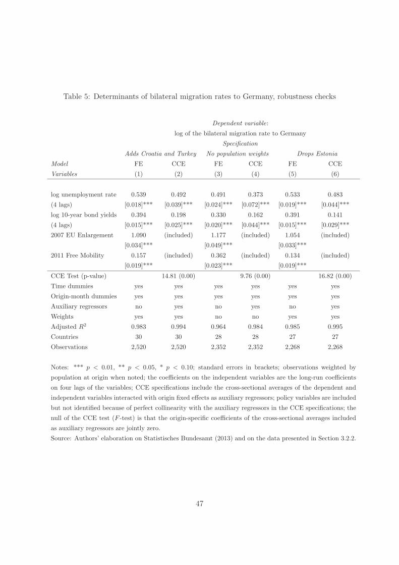
Table 5: Determinants of bilateral migration rates to Germany, robustness checks

Dependent variable:

log of the bilateral migration rate to Germany

Specification

Adds Croatia and Turkey No population weights Drops Estonia

Model FE CCE FE CCE FE CCE

Variables (1) (2) (3) (4) (5) (6)

log unemployment rate 0.539 0.492 0.491 0.373 0.533 0.483

(4 lags) [0.018]*** [0.039]*** [0.024]*** [0.072]*** [0.019]*** [0.044]***

log 10-year bond yields 0.394 0.198 0.330 0.162 0.391 0.141

(4 lags) [0.015]*** [0.025]*** [0.020]*** [0.044]*** [0.015]*** [0.029]***

2007 EU Enlargement 1.090 (included) 1.177 (included) 1.054 (included)

[0.034]*** [0.049]*** [0.033]***

2011 Free Mobility 0.157 (included) 0.362 (included) 0.134 (included)

[0.019]*** [0.023]*** [0.019]***

CCE Test (p-value) 14.81 (0.00) 9.76 (0.00) 16.82 (0.00)

Time dummies yes yes yes yes yes yes

Origin-month dummies yes yes yes yes yes yes

Auxiliary regressors no yes no yes no yes

Weights yes yes no no yes yes

Adjusted R2 0.983 0.994 0.964 0.984 0.985 0.995

Countries 30 30 28 28 27 27

Observations 2,520 2,520 2,352 2,352 2,268 2,268

Notes: *** p < 0.01, ** p < 0.05, * p < 0.10; standard errors in brackets; observations weighted by

population at origin when noted; the coefficients on the independent variables are the long-run coefficients

on four lags of the variables; CCE specifications include the cross-sectional averages of the dependent and

independent variables interacted with origin fixed effects as auxiliary regressors; policy variables are included

but not identified because of perfect collinearity with the auxiliary regressors in the CCE specifications; the

null of the CCE test (F -test) is that the origin-specific coefficients of the cross-sectional averages included

as auxiliary regressors are jointly zero.

Source: Authors’ elaboration on Statistisches Bundesamt (2013) and on the data presented in Section 3.2.2.

47

Table 6: Determinants of bilateral migration rates to Germany, robustness checks (cont’d)

Dependent variable:

log of the bilateral migration rate to Germany

Specification

Population aged 15-49 Two sub-periods Four sub-periods

Model FE CCE FE CCE FE CCE

Variables (1) (2) (3) (4) (5) (6)

log unemployment rate 0.522 0.497 0.465 0.490 0.396 0.462

(4 lags) [0.019]*** [0.043]*** [0.021]*** [0.046]*** [0.028]*** [0.055]***

log 10-year bond yields 0.404 0.138 0.310 0.147 0.213 0.137

(4 lags) [0.015]*** [0.029]*** [0.015]*** [0.030]*** [0.019]*** [0.031]***

2007 EU Enlargement 1.043 (included) 0.821 (included) 0.730 (included)

[0.032]*** [0.028]*** [0.030]***

2011 Free Mobility 0.131 (included) 0.205 (included) 0.172 (included)

[0.018]*** [0.017]*** [0.049]***

CCE Test (p-value) 17.17 (0.00) 6.66 (0.00) 2.82 (0.00)

Time dummies yes yes yes yes yes yes

Origin-month dummies yes yes yes yes yes yes

Origin-sub-period dummies no no yes yes yes yes

Auxiliary regressors no yes no yes no yes

Adjusted R2 0.985 0.995 0.991 0.995 0.994 0.995

Countries 28 28 28 28 28 28

Observations 2,352 2,352 2,352 2,352 2,352 2,352

Notes: *** p < 0.01, ** p < 0.05, * p < 0.10; standard errors in brackets; observations weighted by

population at origin; the coefficients on the independent variables are the long-run coefficients on four lags

of the variables; CCE specifications include the cross-sectional averages of the dependent and independent

variables interacted with origin fixed effects as auxiliary regressors; policy variables are included but not

identified because of perfect collinearity with the auxiliary regressors in the CCE specifications; the null

of the CCE test (F -test) is that the origin-specific coefficients of the cross-sectional averages included as

auxiliary regressors are jointly zero.

Source: Authors’ elaboration on Statistisches Bundesamt (2013) and on the data presented in Section 3.2.2.

48

Appendix

A Further results from the Eurobarometer surveys

Table A.1: Determinants of expectations

Dependent variable:

worse life in general worse economic situation

in the country

Specification

Variables (1) (2) (3) (4) (5) (6)

Unemployment rate 0.473 0.340 0.328 0.231 0.129 0.145

[0.072]*** [0.080]*** [0.097]*** [0.077]*** [0.087] [0.106]

10-year bond yields 0.214 0.2171 0.164 0.167

[0.061]*** [0.062]*** [0.066]** [0.068]**

Gross domestic product -0.115 0.153

[0.528] [0.575]

Adjusted R2 0.849 0.854 0.854 0.606 0.612 0.611

Observations 356 356 356 356 356 356

Countries 26 26 26 26 26 26

Surveys 14 14 14 14 14 14

Country dummies Yes Yes Yes Yes Yes Yes

Time dummies Yes Yes Yes Yes Yes Yes

Notes: *** p < 0.01, ** p < 0.05, * p < 0.10; standard errors in brackets; the dependent variable in

specifications (1)-(3) is the share of respondents who expect their life in general to worsen over the

next year, and in specifications (4)-(6) the share of respondents who expect the economic situation

in their country to worsen over the next year; all variables are in natural logarithms.

Source: Authors’ elaboration on data from European Commission (various issues) and the data

described in Section 3.2.2.

49

Table A.2: Determinants of expectations (cont’d)

Dependent variable:

worse household financial situation worse employment situation

in the country

Specification

Variables (1) (2) (3) (4) (5) (6)

Unemployment rate 0.452 0.222 0.193 0.463 0.414 0.480

[0.065]*** [0.069]*** [0.084]*** [0.091]*** [0.095]*** [0.116]***

10-year bond yields 0.370 0.363 0.080 0.096

[0.052]*** [0.054]*** [0.072] [0.074]

Gross domestic product -0.272 0.632

[0.455] [0.629]

Adjusted R2 0.799 0.826 0.826 0.634 0.635 0.619

Observations 356 356 356 356 356 356

Countries 26 26 26 26 26 26

Surveys 14 14 14 14 14 14

Country dummies Yes Yes Yes Yes Yes Yes

Time dummies Yes Yes Yes Yes Yes Yes

Notes: *** p < 0.01, ** p < 0.05, * p < 0.10; standard errors in brackets; the dependent variable

in specifications (1)-(3) is the share of respondents who expect their the financial situation of their

household to worsen over the next year, and in specifications (4)-(6) the share of respondents who

expect the employment situation in their country to worsen over the next year; all variables are in

natural logarithms.

Source: Authors’ elaboration on data from European Commission (various issues) and the data

described in Section 3.2.2.

50

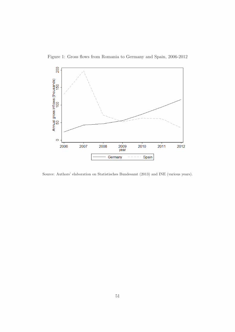
Figure 1: Gross flows from Romania to Germany and Spain, 2006-2012

Source: Authors’ elaboration on Statistisches Bundesamt (2013) and INE (various years).

51

Figure 2: Gross inflows to Germany by country sample, 2006-2016

Source: Authors’ elaboration on Statistisches Bundesamt (2013).

52