FEDERAL RESERVE BANK OF SAN FRANCISCO

WORKING PAPER SERIES

The views in this paper are solely the responsibility of the authors and should not be interpreted as reflecting the views of the Federal Reserve Bank of San Francisco or the Board of Governors of the Federal Reserve System.

Working Paper 2014-10 http://www.frbsf.org/economic-research/publications/working-papers/wp2014-10.pdf

The Euro and the Geography of International Debt Flows

Galina Hale, Federal Reserve Bank of San Francisco

Maurice Obstfeld,

University of California Berkeley, NBER and CEPR

December 2014

The Euro and the Geography of International Debt Flows

Galina Hale∗

Federal Reserve Bank of San Francisco

Maurice Obstfeld

University of California, Berkeley

December 26, 2014

Abstract

Greater financial integration between core and peripheral EMU members not only had aneffect on both sets of countries but also spilled over beyond the euro area. Lower interest ratesallowed peripheral countries to run bigger deficits, which inflated their economies by allowingcredit booms. Core EMU countries took on extra foreign leverage to expose themselves tothe peripherals. We present a stylized model that illustrates possible mechanisms for thesedevelopments. We then analyze the geography of international debt flows using multiple datasources and provide evidence that after the euro’s introduction, core EMU countries increasedtheir borrowing from outside of EMU and their lending to the EMU periphery. Moreover, wepresent evidence that large core EMU banks’ lending to periphery borrowers was linked to theirborrowing from outside of the euro area.

JEL classification: F32, F34, F36

Keywords: international debt, EMU, international banking, global imbalances, euro crisis

∗For helpful comments, we thank four anonymous referees, George Akerlof, Claudia Buch, Eugenio Cerutti, StijnClaessens, Kristin Forbes, Timo Korkemaki, Philip Lane, Luc Laeven, Matteo Maggiori, Alberto Martin, GiovanniDell’Arricia, and participants at the Western Economic Association International 2013 meeting in Tokyo, the October2013 NBER Sovereign Debt and Financial Crisis Conference, the 2014 ASSA meetings, and seminars at Bundesbank,BIS, Swiss National Bank, Univeristy of St. Gallen, Harvard, the FRBSF, the IMF, and the University of Houston.Akshay Rao, Sandile Hlatshwayo, and Peter Jones provided outstanding research assistance. Anita Todd helpedprepare the draft. Obstfeld acknowledges financial support from the Coleman Fung Risk Research Center and Centerfor Equitable Growth at UC Berkeley. All errors are our own. The views in this paper are solely the responsibilityof the authors and should not be interpreted as reflecting the views of the Board of Governors of the Federal ReserveSystem or any other person associated with the Federal Reserve System.

0

1 Introduction

The creation of the European Monetary Union had a large impact on financial flows within the

EMU area. It is well documented that gross debt and equity flows between EMU members in-

creased dramatically as a result of both the single currency and regulatory harmonization within

the European Union (EU).1 Some individual EMU members also began to record larger net finan-

cial inflows in the form of current account deficits, but until the sovereign debt crisis in the EMU

periphery, few observers regarded these as particularly problematic. Only recently has attention

turned to the factors behind these current account deficits as well as the way they were financed

by EMU partners and by countries outside the single currency area.2 Evidence on these questions

is still relatively limited, and studies of the euro’s effect on portfolio positions has tended to focus

on intra-EMU effects. Here we look more broadly and consider the impact of EMU on the global

pattern of gross international financial flows. It is important to understand the worldwide gross

portfolio positions built up in the decade after 1999 because these financed the euro area imbalances

that ultimately led to the euro area crisis.3 In addition, the concentration of peripheral risks on

core EMU lenders’ balance sheets helped to set the stage for the diabolical loop between banks and

sovereigns that has been at the heart of the euro crisis.4

One mechanism generating the big current account deficits of the European periphery could be

summarized as follows: after EMU (and even in the immediately preceding years), compression of

bond spreads in the euro area periphery encouraged excessive borrowing by these countries, domes-

1See Lane (2006), Blank and Buch (2007), Lane and Milesi-Ferretti (2007), Spiegel (2009a), and Pels (2010) forthe evidence on increased gross flows within the euro area and De Santis et al. (2003), Coeurdacier and Martin (2009),De Santis and Gerard (2009), Spiegel (2009b), and Kalemli-Ozcan et al. (2010) for the mechanisms underlying thisdevelopment.

2Trade imbalances of euro area members and their financing are discussed by Chen et al. (2013), who draw on thebilateral international investment position data documented in Waysand et al. (2010).

3Fernandez-Villaverde et al. (2013) review a host of political-economy effects in the euro zone periphery producedby the euro zone credit bubble.

4See Acharya et al. (2011), Brunnermeier et al. (2011), De Grauwe (2012), and Obstfeld (2013) for descriptionsand discussions of this diabolical loop – also known as the “doom loop” or “lethal embrace.”

1

tic lending booms, and asset price inflation.5 We argue that a substantial portion of the financial

capital flowing into the European periphery was intermediated by the countries in the center (core)

of the euro area, inflating both sides of the balance sheet of the large financial institutions in the

core. These gross positions largely took the form of debt instruments, often issued and held by

banks. Thus, EMU contributed not only to the big net deficits of the peripheral countries but also

to inflated gross foreign debt liability and asset positions for core countries such as Belgium, France,

Germany, and the Netherlands – countries that all experienced systemic banking crises after 2007.6

The tendency for systemically important banks to increase leverage in line with balance sheet size

(Miranda-Agrippino and Rey, 2013) implied a substantial increase in financial fragility for these

countries’ financial sectors.7

Four main factors contributed to the suppression of bond yields in the European periphery after

the introduction of the euro. First, the risk of investing in the European periphery declined with

the advent of the euro due to investor assumptions (perhaps erroneous) about future political risks,

including the possibility of official bailouts.8 Second, transaction costs declined and currency risk

disappeared for euro area financial institutions investing in the periphery countries.9 Third, the

European Central Bank’s (ECB’s) policy of applying an identical collateral haircut to all euro area

sovereigns, notwithstanding their varied credit ratings, encouraged additional demand for periphery

sovereign debt by euro area financial institutions (Buiter and Sibert, 2005), which moreover were

able to apply zero risk weights to these assets for computing regulatory capital.10 (The EU’s

5Of course, the extent and form of these phenomena differed among the individual peripheral countries.6See Laeven and Valencia (2013). Shin (2012) describes the role of EMU in encouraging cross-border bank lending

within the euro area.7Brutti and Saure (2013) show evidence consistent with unwinding of this mechanism following the 2008-09 crisis.8Broner et al. (2014) argue that expected preferential treatment of domestic holders of domestic sovereign debt

led to a national home bias in debt holdings after the euro crisis broke out. Analogous expectations might have ledcore euro area lenders to concentrate their risks on euro area borrowers prior to the euro crisis.

9Martin and Rey (2000) model how this reduction in transaction costs affected global equity markets. Hale andSpiegel (2012) show that the decline in transaction costs and currency risk due to the advent of the euro increasedinternational bond issuance in euros relative to the dollar.

10For documentation of similar carry trade behavior after 2007, see Acharya and Steffen (2013). Regarding ECBhaircut policy, Fels (2005) noted: ”[A]t its weekly refinancing operations, the ECB does not discriminate between

2

recent fourth Capital Requirements Directive continues to allow zero risk weights for euro area

sovereign debts, even though the borrowing countries cannot print currency to pay their debts.)

Fourth, financial regulations in the EU were harmonized (Kalemli-Ozcan et al., 2010) and the euro

infrastructure implied a more efficient payment system though its TARGET settlement mechanism.

All four factors seem likely to have given core euro area financial institutions a perceived com-

parative advantage in terms of lending to the periphery, and this would also likely have affected

financial flows from outside to both regions of the euro area. While the preceding considerations

apply to debt flows, including bank loans, they seem less applicable to equity flows, especially

portfolio flows, where the diversification motive is a major driver. We illustrate these mechanisms

in a simple stylized model.

We distinguish our work from earlier studies of the effect of EMU on financial flows by disag-

gregating and differentiating the effects of EMU for core and peripheral euro area countries. In

particular, we examine how EMU changed patterns of both external lending to core and periphery

countries, and lending from core to peripheral countries.

The paper begins by documenting the large increases between 1999 and 2007 in the net foreign

liabilities of the five euro area peripheral countries, Greece, Italy, Ireland, Portugal, and Spain

(the GIIPS), vis-a-vis the rest of the euro area (the “Core”). As is well known, increasing current

account deficits of these heavily borrowing countries were accompanied by a marked suppression in

their government bond spreads relative to the Core. We then describe and analyze the geography

of capital flows and their evolution during the pre-crisis EMU period up to 2007. It is important

to emphasize global trends that act as a backdrop to our analysis — increasing globalization of

financial markets during the time period of our consideration and growing global imbalances. Our

member countries’ debt ratings when accepting bonds as collateral. Therefore, the banking system has no incentiveto discriminate between these bonds, either, because banks can always ship bonds of a lesser credit quality to theECB to obtain liquidity.” As the Buiter-Sibert (2005) analysis also makes clear, collateral quality matters most instates of the world where the borrower defaults on its loan, so a failure to impose borrower-specific haircuts providesa further subsidy to risk taking. For a microeconomic model of ECB refinancing operations, see Cassola et al. (2013).

3

paper does not add to the understanding of these phenomena discussed in the literature (Caballero

et al., 2008; Mendoza et al., 2009), rather, it provides the analysis of relative patterns of gross

financial flows across different regions during this time period.

We exploit two main data sets in our analysis: bank claims from the bilateral BIS data, which

include bank loans as well as banks’ holdings of debt securities, and the loan-level Loan Analytics

data on syndicated bank loans extended by banks and other financial institutions to all types of

borrowers. We analyze patterns of cross-border financial flows in the cross-section setting as well

as in the panel with country pair fixed effects. For both data sets we study the dynamics of stocks

of claims as well as flows.

We find strong evidence of the increase in the financial flows from core EMU countries to the EMU

periphery relative to other regions. We also find that financial flows from financial centers to core

EMU countries increased. In addition, we present bank-specific evidence from the syndicated loan

market that shows a direct link between core EMU banks’ lending to GIIPS and their borrowing

from financial centers. Finally, we present two pieces of circumstantial evidence that are broadly

consistent with the core EMU lenders having a comparative advantage in lending to the GIIPS.

The paper is organized as follows. In Section 2 we give a simplified stylized model of how the

introduction of the euro could have altered the geography of global debt flows. Next, in Section

3 we describe the data that we use. In Section 4 we describe general trends in the data and also

explore the empirical regularities through regression analysis. Section 5 concludes.

2 Trading costs and asset flow diversion

To illustrate potential equilibrium effects following a reduction in peripheral euro zone borrowing

costs, we give an example of a stylized mechanism, the essence of which might drive changes in the

global geography of international debt flows. The example is admittedly extreme, so at the end of

4

the section we discuss more realistic versions of the same basic mechanism.

For the purpose of our example, we can think of the world as consisting of three regions — the

core euro area countries (C), the peripheral euro area countries (P ), and the rest of the world (R).

There is no uncertainty and all lending is accomplished via safe bonds denominated in a single

numeraire. Because the C and the R regions include large financial centers with large trading

volumes, transaction costs of investing between these two regions were always low prior to EMU

and remained so afterward. If we assume in our model that these costs are zero and that capital

can flow freely between the regions, then lenders in C and R will both face the same (gross) global

interest rate r∗.

The transaction costs of lending from either C or R to the P region, however, were relatively

high before EMU because P countries were less integrated into the global capital market. Imperfect

integration was due to a number of factors including currency, financial, and political risks. Thus,

borrowers in P faced a higher interest rate when borrowing from outside the region than the interest

rate prevailing between the C and R regions. We denote the difference by τ .11

To fix ideas, we present a simple project financing model.12 Assume there is a continuum of risk-

neutral agents indexed i in P who each receive 1 unit of endowment that they can either consume

and receive payoff 1 or invest. Investment, however, requires additional 1 unit that agents have to

borrow at a gross interest rate r. Lenders can verify that loaned resources have been invested, so

borrowers cannot divert loans into another use. In case of success, investment brings a payoff of

2R, R > 1, which occurs with agent-specific probability πi. Lenders observe the payoff and can

enforce loan repayment. Otherwise, investment pays 0 and, due to limited liability, the agent does

not have to pay back the loan. Thus, the agent will choose to invest if and only if πi ≥ 1/(2R− r).

11While we refer to the premium charged to P borrowers as transaction costs, one can think of this premium asrepresenting other factors listed in the Introduction.

12This model’s setup is inspired by Martin and Rey (2004) with two main distinctions: we abstract from projectdifferentiation and we assume debt, instead of equity, project financing.

5

Lenders in both C and R regions face the borrowing cost r∗ and a transaction cost τ of lending

to borrowers in P . They are risk-neutral and do not observe any individual borrower’s πi. Thus,

they will be willing to lend if E (πi)r − τ ≥ r∗.

For simplicity, we assume that πi is uniformly distributed on [0, 1] and that lenders know this

distribution and can therefore compute E (πi) conditional on the set of borrowers that are willing

to borrow. In that case, they will be willing to lend at any interest rate greater or equal to

r = 2(r∗ + τ)/(1 + π∗), (1)

where

π∗ = 1/(2R− r) (2)

is the threshold success probability above which agents in P will choose to borrow. Competition

among lenders will drive the interest rate to the level indicated by equation (1).

Solving (1) and (2), we can find equilibrium π∗ and r as a function of R, r∗, τ . It is depicted as

point A on Figure 1, where “Supply” denotes equation (1) and “Demand” denotes equation (2).

Assume that with the introduction of the euro, transaction costs for core EMU lending to the

EMU periphery decline, but remain unchanged (or at least decline by less) for the rest of the

world. In terms of our model, this would be reflected as a decline in τ for banks in C, but not

in R, resulting in their ability to lend to borrowers in P at a lower equilibrium rate. The new

equilibrium rate and threshold π are depicted on Figure 1 as point B. In this new equilibrium, the

interest rate at which funds are available for country P borrowers is lower and more projects are

financed, leading to economic and lending booms in P , just as we observed in the period between

2000 and 2007. Moreover, investment in P now has a lower average probability of success. Lenders

in region R now face higher transaction costs than lenders from region C, so they no longer lend

6

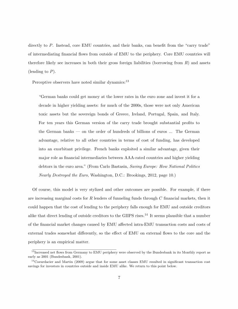
directly to P . Instead, core EMU countries, and their banks, can benefit from the “carry trade”

of intermediating financial flows from outside of EMU to the periphery. Core EMU countries will

therefore likely see increases in both their gross foreign liabilities (borrowing from R) and assets

(lending to P ).

Perceptive observers have noted similar dynamics:13

“German banks could get money at the lower rates in the euro zone and invest it for a

decade in higher yielding assets: for much of the 2000s, those were not only American

toxic assets but the sovereign bonds of Greece, Ireland, Portugal, Spain, and Italy.

For ten years this German version of the carry trade brought substantial profits to

the German banks — on the order of hundreds of billions of euros ... The German

advantage, relative to all other countries in terms of cost of funding, has developed

into an exorbitant privilege. French banks exploited a similar advantage, given their

major role as financial intermediaries between AAA-rated countries and higher yielding

debtors in the euro area.” (From Carlo Bastasin, Saving Europe: How National Politics

Nearly Destroyed the Euro, Washington, D.C.: Brookings, 2012, page 10.)

Of course, this model is very stylized and other outcomes are possible. For example, if there

are increasing marginal costs for R lenders of funneling funds through C financial markets, then it

could happen that the cost of lending to the periphery falls enough for EMU and outside creditors

alike that direct lending of outside creditors to the GIIPS rises.14 It seems plausible that a number

of the financial market changes caused by EMU affected intra-EMU transaction costs and costs of

external trades somewhat differently, so the effect of EMU on external flows to the core and the

periphery is an empirical matter.

13Increased net flows from Germany to EMU periphery were observed by the Bundesbank in its Monthly report asearly as 2001 (Bundesbank, 2001).

14Coeurdacier and Martin (2009) argue that for some asset classes EMU resulted in significant transaction costsavings for investors in countries outside and inside EMU alike. We return to this point below.

7

Some aspects of aggregate data on financial flows are broadly consistent with the mechanism

described by the model. Figure 2 illustrates the well-known fact that EMU led to a compression

of government bond spreads between the Core and Periphery.15 Figure 3 shows that net foreign

liabilities of the GIIPS were increasing mostly vis-a-vis the rest of EMU, while Figure 4 shows that

by 2008 net foreign assets of the Core were mostly vis-a-vis GIIPS and were closely matched by the

liabilities of the Core vis-a-vis the rest of the world. (See also Chen et al. (2013).) However, the

overall picture one derives from gross asset position data is more complex than in our simplified

model.

This complexity is natural once one extends the conceptual framework to encompass additional

uncertainty. Of course, diversification motives provide an explanation for some of the gross two-way

financial flows (especially in equities) that persisted after the euro’s introduction. For that reason,

we focus on debt flows in our empirical analysis below. In addition, in a mean-variance framework

or in a value-at-risk framework such as that of Bruno and Shin (2013), the preceding changes

in expected peripheral returns for Core and rest-of-world lenders could imply portfolio-balance

shifts but not corner solutions, with R lenders reducing but not eliminating their P lending while

simultaneously increasing their lending to C. Indeed, as noted above, it is plausible that the

peripherals’ adoption of the euro somewhat lowered the perceived risks of rest-of-world lending to

them – currency stability even against external currencies was more likely, and the peripherals’

access to core credit and ECB facilities might have reassured external lenders as to the effective

seniority of their own claims. Thus, it would not be surprising to see R claims on P actually rise,

while simultaneously rising on C.

After we describe our data, the remainder of this paper provides more direct evidence on the

effect of EMU on global financial flows.

15Econometric analyses of the pre-crisis convergence of euro area sovereign yields include Ehrmann et al. (2011)and Gerlach et al. (2010).

8

3 Data

An ideal data set for our analysis would consist of all gross debt flows between each country pair,

classified by the nationality as well as the location of the entity extending funds to a borrower.

Unfortunately, such data do not exist. The best information available is for bank lending, at

the country-pair level from the Bank for International Settlements (BIS), and at loan level from

Dealogic.16

The BIS collects data from national central banks on bank claims at the country-pair level. BIS

consolidated banking data series report bank claims by the country in which the global ultimate

owner is headquartered and include all claims of foreign affiliates, while excluding interoffice po-

sitions. These data are available only as stocks for 26 reporting and over 200 vis-a-vis countries

going back to 1983.17 BIS locational banking data classify lenders by residence rather than ulti-

mate ownership and include interoffice positions.18 These series are available as stocks and as flows

(actually, valuation-adjusted stocks, with only exchange rate-related valuation adjustments) for 44

reporting and over 200 vis-a-vis countries going back to 1977. Both types of BIS data omit the

debt holdings of non-bank financial institutions.19

An important difference between BIS consolidated and locational data is how cross-border merg-

ers and acquisitions (M&As) are reflected. M&As in principle would not affect locational data,

16CPIS data from the International Monetary Fund also provides information on the country-pair holdings of debtand equity securities, but due to its locational nature and classification of mutual fund bond investments as equity(Felettigh and Monti, 2008), we find that this data source is not acceptable for our analysis. However, in a recentpaper Hobza and Zeugner (2014) show that similar patterns hold in CPIS data when adjusted for bilateral valuationeffects.

17In this paper we only use BIS consolidated data on immediate borrower basis, because ultimate risk basis data areonly available starting 2005. The difference between these two data sets is in the definition of borrower nationality.In the data we use, the claims are allocated to the country of residence of the immediate borrower. In the ultimaterisk data various risk transfers, such as guarantees, are taken into account and the claims are allocated to the countrywhere the final risk lies (Bank for International Settlements, 2013).

18BIS locational data also include reporting by nationality, rather than by residence, but these data have limitedcoverage.

19In fact, the BIS data are limited to debt holdings of BIS-reporting banks, with a changing coverage of individualbanks over time (Cerutti, 2013).

9

but would change the consolidated data by reassigning the claims held by the target institution to

the acquirer. This change would be reflected by an increase in claims owned by the country of the

acquirer and a decline in claims owned by the country of the target. Thus, changes in consolidated

claims reflect not only actual changes in claims, but also changes in ownership structure of banking

institutions. This is a nontrivial issue in Europe, which saw a number of banking M&As after the

euro’s launch.

In terms of this paper’s hypothesis, M&A might be a relatively low-risk means for banks outside

the euro zone to acquire claims on GIIPS: The acquired bank – even if its owner resides outside

the euro area – might still benefit from cost advantages in lending to the periphery (such as access

to ECB refinancing facilities). For example, a Swedish bank might find it prudent to route loans

to Portugal through an acquired Finnish subsidiary. Consolidated but not locational data would

in this case show financial-center claims on the GIIPS increasing even when direct lending from

financial centers to GIIPS was relatively costly. Of course, any financial-center routing of loans

to GIIPS through subsidiaries in core countries would appear in consolidated data as an increase

in financial-center claims on GIIPS, but could be driven by cost advantages derived from the

subsidiary’s location under the euro area umbrella.

There is one detail of BIS consolidated data that is worth discussing. BIS consolidated data

is presented as cross-border, international, or foreign positions. Cross-border claims series include

only positions for which the lender and the borrower are located in different countries. International

claims series include, in addition, claims by subsidiaries of foreign banks in foreign currencies on

borrowers in the same country. Finally, foreign claims series include, in addition to international

claims series, claims by subsidiaries of foreign banks in local currencies on borrowers in the same

country. While the difference between cross-border and international series tends to be relatively

small, foreign claims are substantially affected by the international bank mergers. For example, if

an Italian bank is acquired by a French bank, all claims of that bank on Italian borrowers become

10

included in foreign claims series, which tends to be a large number because all claims of that Italian

bank were previously viewed as domestic. Also, all foreign currency claims of that bank now become

included in international claim series, but this tends to be a much smaller number. Because we

are trying to capture as much banking flows as possible for our analysis, we do not want to limit

ourselves to cross-border series only. We also want to avoid the large breaks in series in the foreign

claims data that result from international bank mergers. Thus, we choose a middle road and work

with international claims data.

Strictly speaking, a test of our hypothesis would ideally distinguish between lenders whose loans

to the EMU periphery become more profitable after the advent of EMU and those who might benefit

less. Unfortunately, neither the residence not the nationality principle captures the distinction

perfectly. A subsidiary of a U.S. bank in Frankfurt with access to ECB refinancing facilities might

have an advantage in lending to the EMU periphery – and in this case locational rather than

consolidated BIS data would place that lender in the correct category. On the other hand, a

German bank subsidiary residing in New York could likewise have a lending advantage for the

EMU periphery – in which case the consolidated data would get it right. Thus it is useful, in our

view, to look at both locational and consolidated BIS data.

The BIS has recently declassified some of its bilateral data on banking sector claims, both on

locational (by geographical location of each institution) and consolidated (by geographical location

of the headquarters) bases. However, we also have access to the entire set of locational and consol-

idated bilateral data through classified access. As noted earlier, consolidated data allow us to trace

debt flows to the headquarters country of each financial institution.20 Consolidated data, however

have two major shortcomings: first, complete bilateral data are unavailable for euro area countries,

except Greece and Portugal, prior to 1999; second, the consolidated data (as noted above) are not

available in flow form and do not include currency breakdown, which would allow estimation of

20For the importance of intra-institutional transfers, see Cetorelli and Goldberg (2011) and Shin (2012).

11

valuation-adjusted flows. BIS locational statistics, on the other hand, have much more complete

historical coverage, and the BIS provides valuation-adjusted flows using the currency breakdown

of claims.21 We use both data sets and analyze stocks and changes in stocks of total cross-border

claims on all sectors. We deflate all data, reported in U.S. dollars, by the U.S. CPI.

An alternative data source is loan-level data available for syndicated bank loans through Dealogic’s

Loan Analytics. Syndicated lending is of course only a subset of total debt flows. In addition, banks

from several different countries may participate in a syndicate, complicating the attribution of loan

amounts to individual lenders; the data report loan origination, not actual drawdown or repayment

information. Loan Analytics reports the universe of international syndicated loans not only by

banks but also by other financial institutions.22

We classify the nationality of each loan in Loan Analytics based on the nationality of lender

parent, i.e., on a consolidated basis. We use deal nationality to classify the nationality of the bor-

rower. Since the loans are syndicated, they have many lenders, frequently from different countries.

We split each tranche into individual records so that there is only one borrower and one lender per

record. As individual participation amounts are not provided for each lender, we divide the total

tranche amount by the total number of lenders. We divide all the amounts by the U.S. CPI. For

some of the analysis, we aggregate all loan tranches for each lender parent nationality, borrower

nationality, and year to match the structure of the data to that of the BIS data sets. Moreover, we

make use of information on loan type and loan maturity to approximate the amount of syndicated

loan exposures outstanding for each country pair and year, following methodology in Cerutti et al.

(2014). We compute the most conservative exposures by assuming that all loan commitments,

including credit lines, are fully drawn. Thus, both on- and off-balance-sheet commitments are

accounted for, in contrast with BIS data which are limited to on-balance-sheet claims.

21Among previous studies, Blank and Buch (2007) and Kalemli-Ozcan et al. (2010) use BIS locational data, whileSpiegel (2009a) uses the consolidated data.

22See Cerutti et al. (2014) for a detailed comparison of BIS and Loan Analytics data.

12

In order to piece together the most accurate picture possible, we make use of all of the available

data sources, with the understanding that each of them is at best a noisy proxy for the type of

gross debt flows that our hypothesis describes.

For our empirical analysis, we divide the world into four regions. Two regions are GIIPS and

the rest of the euro area, which we label Core (Austria, Belgium, Finland, France, Germany,

Netherlands, Luxembourg, and Finland).23 We separate the rest of the world into two groups.

The first group includes the rest of the EU and large reporting financial centers (Fin): Canada,

Denmark, Japan, Sweden, Switzerland, the U.K., and the U.S. The second group consists of all

remaining countries (ROW).24

Some banks appear as both borrower and lender parents in Loan Analytics. We isolate 51 banks

(large global banks and banks included in the European Banking Authority (EBA) stress tests that

are active in the syndicated loan market), which account for about 84 percent of total syndicated

lending. Of these banks, 23 are in the core EMU. This allows bank-level analysis of borrowing and

lending patterns. In addition, we use information on syndicate structure for supplemental testing.

4 Geography of international debt flows

We first present our analysis of country-pair level data to evaluate the effect of EMU on patterns

of global financial flows, then we turn to bank-level regressions. We also discuss some evidence

23We do not have Cyprus and Malta in our data set. Slovenia and the Slovak Republic are coded as ROW becausethey joined EMU in 2007 and 2009, respectively.

24The sample of countries in ROW varies depending on the data source we use. It generally includes advancedeconomies as well as emerging markets. For BIS data sources, we limit the set of countries to the BIS-reporting coun-tries available through confidential data access so that the same set of countries appear as borrowers and lenders. Forconsolidated data the 10 ROW countries are Australia, Brazil, Chile, Hong Kong, India, Mexico, Panama, Singapore,Taiwan, and Turkey. For locational data there are 31 ROW countries: Argentina, Australia, Brazil, Bulgaria, Chile,China, Czech Republic, Egypt, Hong Kong, Hungary, India, Indonesia, Malaysia, Mexico, New Zealand, Norway,Peru, Philippines, Poland, Romania, Russia, Slovak Republic, Slovenia, South Africa, South Korea, Taiwan, Thai-land, Turkey, Ukraine, Venezuela, and Vietnam. Loanware data include many countries, but for consistency we limitthe set of ROW countries to be the same as in locational BIS data. All panels are unbalanced.

13

supporting the hypothesis of a comparative advantage of Core lending to GIIPS after 1999. Given

the limitations of the data, we cannot test directly for the mechanism underlying patterns of

international debt flows. We do, however, present two pieces of circumstantial evidence consistent

with our hypothesis.

4.1 Bilateral lending dynamics

We begin by documenting percentage changes in country-pair stocks of bank claims, in real U.S.

dollars, during the EMU time period. Figure 5 is a heat map that shows these percentage changes

for BIS locational and consolidated data. The figures show the matrix of bilateral positions of EMU

countries, Switzerland, the U.K., and the U.S.25 It is apparent that lending from all countries to

Switzerland, the U.K. and the U.S. declined or increased much less than lending to EMU countries.

Among EMU countries, Netherlands, Greece, Ireland, Portugal, and Spain experienced the biggest

increases in debt inflows from most countries. Comparing the two panels, we see a few examples

illustrating important differences between consolidated and locational BIS data. For example, the

increase in U.K. lending to core EMU countries was very large if measured using consolidated data,

but not if using locational data. This is because much U.K. lending to core EMU countries took

place through British subsidiaries residing abroad.

We next examine how the geographical composition of international lending and borrowing

changed relative to positions accumulated prior to EMU. Figure 6 shows banking claims using

BIS (both consolidated and locational) data across four regions: financial centers (FIN), the core

Euro area (CORE), the GIIPS, and the rest of the world (ROW). The left-hand-side of the chart

presents each regions’s stock of claims at the beginning of EMU vis-a-vis another region, with the

thickness of the lines reflecting holdings, measures in real USD, as a share of global gross positions,

also measured in real USD. The right-hand-side of the chart presents changes in gross positions

25See Zucman (2013) for a detailed discussion of the special role of Switzerland in European finance.

14

from the beginning of the EMU period through the end of 2007, in real USD, scaled by the global

change in gross positions in real U.S. dollars over this same time period. In interpreting these

charts, we view the stocks of claims at the beginning of EMU as a reflection of flows that occurred

prior to EMU.

The top panel maps the claims of the banking system using consolidated BIS data. Here we

see very clearly a substantial increase in flows from FIN to CORE relative to what we observed

prior to EMU. We also see an increase in banking flows from CORE to GIIPS. Lending from

financial centers to the GIIPS also goes up noticeably after 1999, indicating an overall increase in

the attractiveness of GIIPS assets even for countries outside of EMU. As we observed in Figure 5,

much of this lending went to the housing boom countries, Spain and Ireland.

The bottom panel shows the claims of the banking system using locational BIS data. Here we

also observe an increase in banking flows from CORE to GIIPS relative to the flows accumulated

prior to EMU. We see, however, a less pronounced increase in flow from FIN to CORE, which is

more than compensated by an increase in flows from CORE to FIN, indicating that the increase in

lending that we observed with consolidated data was largely due to lending by foreign subsidiaries of

financial center banks. This is confirmed by lower increases in FIN lending to GIIPS for locational

relative to consolidated data documented in Figure 5.

To see whether the regional patterns are driven by specific countries, we turn to Figure 7. The top

panel of Figure 7 is based on the BIS consolidated data and the bottom panel on BIS locational data.

We compute the share of total lending to GIIPS by individual Core countries in each country’s total

lending (left column), and the share of Core in total borrowing by each country from GIIPS in each

country’s total borrowing (right column).26 Looking at consolidated data we find that there was an

increase in bank lending, especially for Austria, France, and Germany, with France experiencing an

26In computing total lending we only include lending and borrowing countries in our sample. Excluded countriesonly contribute a small share of either borrowing or lending, and the charts would look virtually the same if weinclude all countries.

15

increase earlier during the EMU period than Germany. We don’t see a clear increase in the share

of Core banks in total borrowing by GIIPS, with the exception of Greece, and to a lesser extent,

Portugal. Locational BIS data show patterns broadly similar to and more pronounced than those

we observe with consolidated statistics. We do not observe an increase in the share of lending to

GIIPS by banks residing in Austria, indicating that Austrian-owned banks increased the share of

lending to GIIPS through their foreign subsidiaries.

To formalize the analysis of Figures 5 to 7, we present estimates for a set of cross-sectional

regressions based on the bilateral (country-pair) framework that has been used by Portes and Rey

(2005), Lane (2006), Coeurdacier and Martin (2009), and other authors. For each country-pair we

compute a change in the log of real USD claims between 1999 and 2007 for BIS consolidated (BISC)

and locational (BISL) data. For the BIS locational data, we also sum up the valuation-adjusted

flows (BISLF) in 1999-2007 in real USD and control for the stocks of claims in 1999.27 We also

conduct this analysis for the syndicated loan market, using two representations of the Dealogic data.

First, using information on loan maturity, we compute total syndicated loan exposures (SLEC) of

each country i to each country j at the end of each year, a stock variable that is similar to the BIS

claims variable. Since we use lender parent nationality, this is most analogous to the consolidated

BIS data. We then compute the change in log of real USD syndicated loan exposures between

1999 and 2007. Alternatively, we sum up all loans extended by lenders in country i to borrowers

in country j in a given year, which is a flow of loan origination (LW).28 We sum up these flows for

the years 1999-2007 and control for the exposures at the end of 1999, as with BIS locational flow

regression.

The results of this analysis are presented in Table 1, with column (1) showing the results for the

BIS consolidated data, columns (2) and (3) showing the results for the BIS locational data stocks

27We also experimented with computing the differences between BIS locational and consolidated claims for eachcountry to proxy for lending intermediated by affiliates but did not observe any significant patterns.

28We do not have information on loan repayments or drawdowns, and therefore cannot compute actual loan flows.

16

and flows, respectively, and columns (4) and (5) showing the results for the syndicated loan data

exposures and origination flow. In the regressions with stocks, the left-hand side variable is unit-free

— percentage change in stocks during indicated time period. In contrast, in regressions with flows,

the left-hand side variable is unscaled accumulation of flows in real USD. Therefore, for the flow

regressions, we include initial stock on the right-hand side as a control variable.29 Given that the

only explanatory variables in these regressions, with the exception of initial stocks, are indicator

variables, these regressions are basically comparisons of means that demonstrate magnitudes and

statistical significance of differences across region pairs. The unit of observation in these regressions

is a country pair.

We focus on region pairs that drew our attention in analyzing Figure 6. We include indicators

for region pairs: CORE lending to FIN and to GIIPS, and FIN lending to CORE and to GIIPS,

with the omitted category being lending between all other region pairs.30 We find that, relative to

all other country pairs, there was a pronounced increase in lending from CORE to GIIPS across all

measures, although for syndicated loan origination it was not statistically significant. In all cases,

except for the consolidated BIS regression, we also find a substantial increase in lending from FIN

to CORE. Thus, regressions provide support from the discussion of graphical evidence.31 For BIS

locational data we also observe an increase in lending from FIN to GIIPS. Interestingly, we also

find that claims of CORE banks on FIN borrowers have fallen relative to other region pairs during

this time period, suggesting that CORE banks likely diverted their lending from FIN to GIIPS.

However, this is not true for the syndicated loan market, where CORE to FIN lending actually

29We attempted to include additional control variables: housing price growth differentials, interest rate differentials,gravity-type measures such as geographical distance and common language, as well as indicators of trade blocks: EMU,NAFTA, ASEAN. These variables did not enter significantly and did not affect our results. In the robustness testswe established that controlling for trade flows also leaves our results mostly unchanged.

30We experimented with including lending from GIIPS to CORE and from GIIPS to FIN among region pairs. Theresults of these tests and of various permutations of region definitions are discussed in Section 4.4. The bottom lineis that the main coefficients of interest are robust to such changes.

31The fact that we do not observe this increase in the consolidated BIS data suggests that some of the lending fromFIN to CORE was due to lending by foreign banks located in the FIN region, potentially European banks.

17

increased relative to other regions. Note that within-region differences across country pairs must

be large, because the explanatory power of the stock regressions is very low.

The magnitudes of the differences across regions are substantial, but plausible. In order to see

this, note that the left-hand side is a change in the natural logarithm of the stock variable (with

the exception of the BIS locational flows and loan origination regressions), while the variables of

interest are 0/1 indicators. Thus, 100 ∗ (eβ − 1) gives us a percentage difference between the region

pair examined and the excluded set of region pairs. For example, we find that the increase in total

stock of bank claims between 1999 and 2007 as measured by the change in BIS locational stocks

(column (2)) was 93 percent for the excluded group,32 198 percent for claims of CORE on GIIPS,

and 102 percent for claims of FIN on CORE.

We next turn to the country-pair by year panel data analysis, similar to the approach taken by

Blank and Buch (2007) and Spiegel (2009b). We test whether the flows for the pairs of regions that

we discuss have changed substantially after 1999. To do so, we interact indicators of region pairs

with an indicator of the pre-crisis EMU time period. We estimate regressions with country-pair

and year fixed effects so that our identification comes from changes within country pairs.33 We also

control for the total amount lent and total amount borrowed by each country in each year to account

for all potential country-specific push and pull factors. Because consolidated BIS data for EMU

countries are not available prior to 1999 (except for Portugal and Greece), our analysis is limited to

BIS locational data. We supplement this analysis with syndicated loan issuance aggregated from

the loan-level data using the Loan Analytics data set, with its exposure and origination versions,

as before.

The results are presented in Table 2. We find that, following the introduction of the euro, claims

of CORE on GIIPS have increased by about 60 percent in the case of BIS data and by 20-30 percent

32Obtained as 100 ∗ (eCONSTANT − 1).33Note that including country-pair fixed effects addresses some of the criticism raised by Okawa and Van Wincoop

(2012) for gravity-type models of international capital flows.

18

for syndicated lending. With the exception of the BIS stock data, we also see an increase in lending

from FIN to CORE after the introduction of the euro, by about 50 percent in the case of BIS flows

and by 80 percent in the syndicated loan market. We continue to find evidence of an increase in

direct lending from FIN to GIIPS, although this is only reflected in flow measures. We also find

increased syndicated lending from CORE to FIN after the introduction of the euro.

To summarize the results of Tables 1 and 2, we find that during the pre-crisis EMU period there

was a pronounced and statistically significant increase in debt flows from core EMU to GIIPS,

relative to other region pairs. This increase is observed in all data sources we use, regardless of

their representation (stocks or flows). We also find a substantial increase in lending from FIN to

CORE, especially in the syndicated loan market. These two findings, however, do not prove that

there was a link between lending provided to GIIPS by financial institutions in CORE and lending

by financial institutions in FIN to CORE. To show this link, we now turn to bank-level analysis.

4.2 Bank-level evidence

The only comprehensive and accessible source of data on the geographical composition of borrowing

and lending by individual banks is the Loan Analytics database. Top banks appear as both lenders

and borrowers in these data, allowing us to see how the geography of their lending is related to

the geography of their borrowing. Even though syndicated lending from CORE to GIIPS is rather

limited, we examine whether there is a correlation between banks’ lending to GIIPS and these same

banks’ borrowing from FIN. For at least some large banks we definitely see this link, as shown in

Figure 8.34

To test whether this link between core EMU banks’ borrowing from financial centers and their

lending to GIIPS is a more widespread phenomenon, we isolate 52 banks — either large global

34These banks are systemically large: Bayern and Deutsche Bank’s assets were 17 and 82 percent of Germany’sGDP, ING Group’s assets were 212 percent of Netherlands’ GDP, and Reiffeisen’s assets were 38 percent of AustrianGDP, all as of the end of 2011.

19

banks or banks included in EBA stress tests — that are active on the syndicated loan market.

These banks account for about 84 percent of total syndicated lending. Of these banks, 23 are in

the core EMU, 11 are in FIN, and 13 are in GIIPS.35 For these banks, we collect information on

syndicated lending to them from different regions as well as their own participation in syndicated

lending by region. We then estimate the regression of the amount lent to GIIPS as a function of the

amount borrowed from different regions, and allow for the effect to change after the introduction of

the euro. The results are reported in Table 3. In column 1 the sample is limited to financial center

banks, in column 2 to core EMU banks, and in column 3 to periphery banks. In all regressions we

control for the total amount lent and borrowed through the syndicated loan market by each bank,

as well as for bank and year fixed effects.

The results in Table 3 show that, controlling for total borrowing and lending by each bank in

each year, only for CORE banks is there an increased link between their borrowing from FIN and

their lending to GIIPS during the pre-crisis EMU period – a roughly one-to-one increase. We do

not find such a link for banks from other regions. In addition, we find that financial center and

GIIPS banks, but not Core banks, seem to have been intermediating flows from ROW to GIIPS.36

This finding is expected, in that the ROW lenders are likely to be facing even larger transaction

and information costs in lending directly to GIIPS than do the financial center banks.

4.3 Additional evidence

We suggested several reasons why the core EMU lenders might have had a comparative advan-

tage over financial centers in lending to the GIIPS. So far, we demonstrated a reorientation of

global capital flows beyond an increase in CORE lending to GIIPS. We believe this comparative

advantage caused not only greater lending from the CORE to the GIIPS, but also more lending

35The list of banks is provided in the footnote to Table 3.36The ROW countries that lend to GIIPS banks in this sample are Australia, China, Egypt, Hong Kong, Israel,

Malaysia, Norway, Panama, Singapore, Korea, Taiwan, and Turkey, as well as Middle East and offshore financialcenters.

20

from FIN to CORE and possibly less lending by FIN to GIIPS. While testing for the mechanisms

underlying these dynamics is impossible due to data limitations, we provide two pieces of evidence

that are consistent with the premises we brought forth in discussion of the comparative advantage

mechanism.

First we show that the collateral advantage that the ECB gave to the euro area sovereign bonds

had an effect that spread beyond the euro area. To do this, we use data on syndicated lending

to sovereigns. Since syndicated loans to sovereigns did not have the same collateral advantages as

sovereign bonds, GIIPS sovereigns found it cheaper to borrow through the debt market. Indeed, we

observe a sharp decline in syndicated lending from CORE to GIIPS sovereigns at the start of the

EMU period. While overall syndicated lending from CORE banks to GIIPS increased throughout

this time period, lending to sovereigns dropped nearly to zero, resulting in a sharp drop of the

share of sovereign borrowers in total syndicated lending to GIIPS in the early 2000s (Figure 9).

This was not the case for the rest of the market — while there is a downward trend in the share

of lending to sovereigns in all countries in total lending to all countries, this share did not drop to

zero. We also note that syndicated lending to GIIPS sovereigns by lenders outside the euro area

also dropped to zero once a cheaper form of financing became available to them. Thus, we observe

that the ECB collateral policy (one of the four factors contributing to the core EMU comparative

advantage) indeed had an effect.

Next, we study regional composition of loan syndicates to provide evidence that FIN lenders

found GIIPS borrowers relatively less attractive after the introduction of the euro. To do so, we

estimate linear probability regressions of an indicator that there is at least one bank from FIN in

the syndicate for all loans, for loans in which at least one bank is from CORE, for all loans to

GIIPS, for loans to GIIPS in which at least one bank in the syndicate is from CORE, and for all

loans to CORE. As controls we included deal amounts, number of lenders in the syndicate, and

21

year fixed effects.37

Figure 11 shows a plot of the estimated year fixed effects from these regressions.38 We find

that while there was not much change in the regional composition of loan syndicates in the deals

extended to other regions, there was a sharp drop during the EMU period in the probability of a

FIN bank participating in lending to GIIPS, whether or not a CORE bank is also in a syndicate.39

One potential explanation for this dynamics is that, consistently with our argument, FIN banks

were no longer as active in arranging syndicated loans to GIIPS and their share of origination was

replaced by CORE banks. As Figure ?? shows by depicting the shares of loans with at least one

lead arranger from FIN and from GIIPS, this was indeed the case. It is possible that in addition,

CORE banks originating loans to GIIPS were not as likely to invite FIN banks to participate after

1999, fearing that inclusion of EMU outsiders in the syndicate might reduce the likelihood of a

bailout by the European authorities.

4.4 Other regional patterns and robustness tests

In the above analysis we relied on the groupings of countries into regions. While the definitions of

the core euro area and GIIPS are conventional, the choice of countries included in FIN is somewhat

arbitrary and there is no a priori reason to believe that they represent a homogeneous group.

The same can be said for the ROW countries. For this reason, and to gain additional insight into

changes in the geography of debt flows brought about by the EMU, we conduct some additional

tests. In the interest of space we do not report all regressions, but summarize their results.40

United Kingdom

37In the interest of space, we do not report the regressions themselves.38Here we only observe the syndicate composition at the time of loan origination. As Ivashina and Scharfstein

(2010) stress, composition of loan syndicates can change during the life of a loan.39These dynamics are not explained by the increased number of loans extended to GIIPS, which did not occur

until 2004.40Regression results are available upon request.

22

Our first concern is that the European Union banks outside the euro zone might have considerable

advantage over banks outside the EU. There are two main reasons for this: first is the general

harmonization of banking rules in the EU; second is the fact that some EU banks outside the euro

zone have access to ECB lending facilities. The most important set of non-euro zone EU banks

resides in the U.K., which we include among the financial centers, but which may behave differently

than banks from the U.S. or Japan.

For locational BIS data, it is especially important to note that there are many foreign-owned

banks in the U.K., and these happen to be banks that are internationally active. Lending to Irish

banks, in particular, is frequently channeled from core EMU banks through their London branches

and will therefore be reported as lending from financial centers to GIIPS in any data that are based

on the residence principle. This problem is less important for the BIS consolidated data and the

Loan Analytics data, which are reported on a nationality basis. However, it might be important

to separate the U.K. for the analysis of the syndicated loans, since London is a central hub for

international syndicated lending.

Thus, we separate the U.K. from the rest of the FIN group and re-estimate our regressions in

Tables 1 and 2 with addition of UK to CORE, UK to GIIPS, and CORE to GIIPS dummies,

thus leaving the benchmark unchanged. We find that the coefficients on CORE to FIN, FIN to

CORE, and FIN to GIIPS are surprisingly unchanged, both in terms of statistical significance and

in terms of magnitude.41 If anything, we now observe a larger relative increase in lending from FIN

to CORE and FIN to GIIPS, by 134 and 144 percent, respectively, in the cross-section regression.

In all specifications we observe a large increase in lending from UK to both CORE and GIIPS,

with magnitudes comparable to or higher than the increase in lending from FIN to CORE and to

GIIPS. The results are even less affected in the panel regression, suggesting that the UK is not

that different from the rest of the FIN group and including the UK into the FIN group is not what

41Obviously, coefficients on CORE to GIIPS are unaffected by construction.

23

drives the results.

United States

Similarly, the position of the U.S. in the global financial markets is known to be unique. We

separate the US from the rest of the FIN group in the same way and return the U.K. back to

this group. The coefficients on FIN to CORE and FIN to GIIPS, as well as CORE to FIN are

remarkably similar. In addition, we find an increase in lending from the U.S. to CORE in all but

BIS consolidated regressions in the cross-section. This suggests that some of the increase in lending

from the U.S. to CORE was conducted by affiliates of foreign institutions located in the U.S. We

do, however, observe an increase in syndicated lending by U.S. banks to CORE borrowers. Overall,

our alterations of the FIN group of countries do not produce substantial changes in the results,

indicating that, surprisingly, the FIN group is sufficiently homogeneous in terms of our analysis.

Central and Eastern Europe

During the sample period that we are focusing on, substantial changes were observed in financial

flows to Central and Eastern Europe (CEE),42 especially countries that were preparing to join the

EMU. Much of the lending to these economies was provided by banks in Germany and Austria.

For this reason, it might be useful to separate lending from CORE to CEE from the benchmark

category. Unfortunately, we cannot estimate this regression with BIS consolidated data because we

do not have information on lending to CEE countries. For the rest of the regressions we find that

the coefficients on other region pairs remain basically unchanged and that in most specifications

we observe a relative increase in lending from CORE to CEE borrowers, as one would expect.

42Countries in our sample that we categorize as CEE are Bulgaria, Russia, Ukraine, Czech and Slovak Republics,Hungary, Slovenia, Poland, and Romania.

24

Rest of Europe

In addition to the UK and the US, the FIN group is comprised of Japan and other European

countries: Denmark, Sweden, and Switzerland (DSS). We can conduct a similar exercise and sep-

arate these countries from the rest of the FIN group and estimate their lending to GIIPS and to

CORE, as well as to CEE. For completeness, we also add an indicator for loans from remaining

countries in the FIN group to DSS.43 We find that differences in the coefficients on the remaining

FIN group are substantially different only in a couple of specifications and are overall quite different

from those of CORE banks. Moreover, we only find an increase in lending from DSS to CORE in

the syndicated loan market, but not in the BIS data. Changes in lending by DSS to GIIPS and to

CEE as well as in lending from FIN to DSS are not consistent across data sets and specifications.

These results, along with those for the U.K. discussed above, show that banks located in European

countries outside of the euro area behaved quite differently than banks in the CORE, confirming

that the comparative advantage increase for CORE was specific to the effect of the euro and not

merely the effect of the EU.

GIIPS lending

Our next exercise is to separate lending from GIIPS to CORE and to FIN from the benchmark

group. Since it is affecting the benchmark group, this change may affect the coefficients on region

pairs of interest. In practice, however, the differences are very small. In addition, we observe a

large and statistically significant relative increase in lending from GIIPS to both CORE and FIN

regions, with the exception of cross-section regression with BIS locational flows.

Robustness tests

43We found that if we include UK alongside Denmark, Sweden, and Switzerland in the group, the results wereessentially the same.

25

We conducted a series of robustness tests in addition to those described above. In terms of

countries included in the analysis, we tested whether the inclusion of Luxembourg (which we

excluded from the main specification due to its special status as a financial center) or exclusion of

Ireland (which had close financial ties with the UK) affect our results and found that this was not

the case. We also tested to see whether the inclusion of Italy in GIIPS was driving all the results

and found that this is not the case either: excluding Italy from GIIPS does not change the results.

We also attempted to control for trade flows for each country pair and found that, while trade flows

do have significant impacts on financial flows in some specifications, including them does not alter

the rest of the results.

5 Conclusion

The big current account deficits of peripheral euro area countries reflected an accumulation of

problems that have led to instability in the euro area. In this paper we analyze the patterns of

international debt flows that financed and potentially amplified the accumulation of these imbal-

ances. Not only did peripheral countries borrow more after EMU was established; in addition,

financial institutions in the core of the euro area expanded their balance sheets to facilitate pe-

ripheral deficits, thereby increasing their own fragility. This pattern set the stage for the diabolical

feedback loop between banks and sovereigns that has been such a powerful driver of the euro area’s

recent crisis.

The findings raise important questions for future research, questions that would have to be pur-

sued at a more granular level with respect to both lenders and borrowing countries. Can we identify

the precise mechanisms promoting heavy lending from the EMU core to the EMU periphery dur-

ing the euro’s first decade, and which were most important quantitatively? Acharya and Steffen

(2013) have made some progress on similar questions using recent data from the European Banking

Authority stress tests. To what extent did peripheral countries differ in their borrowing behavior?

26

Before 2009, the peripheral economies showed considerable diversity in terms of financial infras-

tructure, government deficits, and asset-price developments. How did these differences affect their

demands for loans from abroad, as well as their own investments in foreign countries? We leave

these questions to be answered in future research.

27

References

Acharya, Viral V., Itamar Drechsler, and Philipp Schnabl. A Pyrrhic Victory? Bank Bailouts andSovereign Credit Risk. NBER WP 17136, 2011.

Acharya, Viral V. and Sascha Steffen. The Greatest Carry Trade Ever? Understanding EurozoneBank Risks. NBER WP 19039, 2013.

Bank for International Settlements. Guidelines for reporting the BIS international banking statis-tics. Monetary and Economic Department, 2013.

Blank, Sven and Claudia M. Buch. “The Euro and Cross-Border Banking: Evidence from BilateralData.” Comparative Economic Studies 49 (2007): 389–410.

Broner, Fernando, Aitor Erce, Alberto Martin, and Jaume Ventura. “Sovereign Debt Markets inTurbulent Times: Creditor Discrimination and Crowding-Out Effects.” Journal of MonetaryEconomics 61 (2014): 114–142.

Brunnermeier, Markus, Luis Garicano, Philip R. Lane, Marco Pagano, Ricardo Reis, Tano Santos,Stijn van Nieuwerburgh, and Dimitri Vayanos. European Safe Bonds (ESBies). URL: http://euro-nomics.com/wp-content/uploads/2011/09/ESBiesWEBsept262011.pdf, 2011.

Bruno, Valentina and Hyun Song Shin. Capital Flows, Cross-Border Banking and Global Liquidity.NBER WP 19038, 2013.

Brutti, Filippo and Philip Saure. Repatriation of Debt in the Euro Crisis: Evidence for theSecondary Market Theory. Mimeo, 2013.

Buiter, Willem and Anne Sibert. How the Eurosystem’s Treatment of Collateral in Its Open MarketOperations Weakens Fiscal Discipline in the Eurozone (and What to Do about It). CEPR DP5626, 2005.

Bundesbank. Monthly Report. March, 2001.

Caballero, Ricardo J., Emmanuel Farhi, and Pierre-Olivier Gourinchas. “An Equilibrium Model of“Global Imbalances” and Low Interest Rates.” American Economic Review 98 (2008): 358–393.

Cassola, Nuno, Ali Hortacsu, and Jakub Kastl. “The 2007 Subprime Market Crisis through the Lensof European Central Bank Auctions for Short-Term Funds.” Econometrica 4 (2013): 1309–1345.

Cerutti, Eugenio. Banks’ Foreign Credit Exposures and Borrower’s Rollover Risks Measurement,Evolution and Determinants. IMF WP 13/9, 2013.

Cerutti, Eugenio, Galina Hale, and Camelia Minoiu. “Financial Crises and the Composition ofCross-Border Lending.” Journal of International Money and Finance forthcoming (2014).

Cetorelli, Nicola and Linda Goldberg. “Global Banks and International Shock Transmission: Evi-dence from the Crisis.” IMF Economic Review 59 (2011): 41–76.

28

Chen, Ruo, Gian Maria Milesi-Ferretti, and Thierry Tressel. “External Imbalances in the EuroArea.” Economic Policy (2013).

Coeurdacier, Nicolas and Philippe Martin. “The Geography of Asset Trade and the Euro: Insidersand Outsiders.” Journal of Japanese and International Economics 23 (2009): 90–113.

De Grauwe, Paul. “The Governance of a Fragile Eurozone.” Australian Economic Review 45(2012): 255–268.

De Santis, Giorgio, Bruno Gerard, and Pierre Hillion. “The Relevance of Currency Risk in theEMU.” Journal of Economics and Business 55 (2003): 427–62.

De Santis, Roberto A. and Bruno Gerard. “International Portfolio Reallocation: DiversificationBenefits and European Monetary Union.” European Economic Review 53 (2009): 1010–1027.

Ehrmann, Michael, Marcel Fratzscher, Refet S. Gurkaynak, and Eric T. Swanson. “Convergenceand Anchoring of Yield Curves in the Euro Area.” Review of Economics and Statistics (2011):350–364.

Felettigh, Alberto and Paola Monti. “How to interpret the CPIS data on the distribution of foreignportfolio assets in the presence of sizeable cross-border positions in mutual funds. Evidence forItaly and the main euro-area countries.” Banca d’Italia Occasional papers 16 (2008).

Fels, Joachim. Of Bubbles, Complacency, and Liquidity. Morgan Stanley Global Economic Forum,January 25, 2005.

Fernandez-Villaverde, Jesus, Luis Garicano, and Tano Santos. “Political Credit Cycles: The Caseof the Eurozone.” Journal of Economic Perspectives 27 (Summer 2013): 145–166.

Gerlach, Stefan, Alexander Schulz, and Guntram B. Wolff. Banking and Sovereign Risk in the EuroArea. CEPR Discussion Paper 7833, 2010.

Hale, Galina B. and Mark M. Spiegel. “Currency Composition of International Bonds: The EMUEffect.” Journal of International Economics 88 (2012): 134–149.

Hobza, Alexandr and Stefan Zeugner. “Current accounts and financial flows in the euro area.”Journal of International Money and Finance 48 (2014): 291–313.

Ivashina, V. and D. Scharfstein. “Loan Syndication and Credit Cycles.” American EconomicReview 100 (2010): 57–61.

Kalemli-Ozcan, Sebnem, Elias Papioannou, and Jose Luis Peydro. “What Lies Beneath the Euro’sEffect on Financial Integration? Currency Risk, Legal Harmonization or Trade.” Journal ofInternational Economics 81 (2010): 75–88.

Laeven, Luc and Fabian Valencia. “Systemic Banking Crises Databse.” IMF Economic Review 61(2013): 225–270.

29

Lane, Philip R. “Global Bond Portfolios and EMU.” International Journal of Central Banking 2(2006): 1–23.

Lane, Philip R. and Gian Maria Milesi-Ferretti. “The International Equity Holdings of EuroArea Investors.” The Importance of the External Dimension for the Euro Area: Trade, CapitalFlows, and International Macroeconomic Linkages. Ed. Robert Anderton and Filipo di Mauro.Cambridge, UK: Cambridge University Press, 2007.

Martin, Philippe and Helene Rey. “Financial integration and asset returns.” European EconomicReview 44 (2000): 1327–1350.

Martin, Philippe and Helene Rey. “Financial super-markets: size matters for asset trade.” Journalof International Economics 64 (2004): 335–361.

Mendoza, Enrique G., Vincenzo Quadrini, and Jose-Vctor Rıos-Rull. “Financial Integration, Finan-cial Development, and Global Imbalances.” Journal of Political Economy 117 (2009): 371–416.

Miranda-Agrippino, Silvia and Helene Rey. World Asset Markets and Global Liquidity. Mimeo,2013.

Obstfeld, Maurice. Finance at Center Stage: Some Lessons of the Euro Crisis. European EconomyEconomic Papers 493, April 2013.

Okawa, Yohei and Eric Van Wincoop. “Gravity in International Finance.” Journal of InternationalEconomics 87 (2012): 205–215.

Pels, Barbara. International Asset Holdings and the Euro. IIIS Discussion Paper No. 331, 2010.

Portes, Richard and Helene Rey. “The Determinants of Cross-Border Equity Flows.” Journal ofInternational Economics 65 (March 2005): 269296.

Shin, Hyun Song. “Global Banking Glut and Loan Risk Premium.” IMF Economic Review 60(2012): 155–192.

Spiegel, Mark M. “Monetary and Financial Integration: Evidence from the EMU.” Journal of theJapanese and International Economies 23 (June 2009): 114–130.

Spiegel, Mark M. “Monetary and Financial Integration in the EMU: Push or Pull?.” Review ofInternational Economics 17 (2009): 751–776.

Waysand, Claire, Kevin Ross, and John C De Guzman. European Financial Linkages: A New Lookat Imbalances. IMF WP/10/295, 2010.

Zucman, Gabriel. “The Missing Wealth of Nations: Are Europe and the U.S. Net Debtors or NetCreditors?.” Quarterly Journal of Economics 128 (2013): 1321–1364.

30

Figure 1: Equilibrium lending before and after EMU

Demand

Supply

Supply

A

B

r

π

(low τ)

Equations (1) and (2) plotted for R = 1.2, r∗ = 1.05, τ = 0.1, low τ = 0.

31

Figure 2: Government bond spreads between GIIPS and Core

‐10

‐5

0

5

10

15

20

25

30

1993:Q1

1993:Q3

1994:Q1

1994:Q3

1995:Q1

1995:Q3

1996:Q1

1996:Q3

1997:Q1

1997:Q3

1998:Q1

1998:Q3

1999:Q1

1999:Q3

2000:Q1

2000:Q3

2001:Q1

2001:Q3

2002:Q1

2002:Q3

2003:Q1

2003:Q3

2004:Q1

2004:Q3

2005:Q1

2005:Q3

2006:Q1

2006:Q3

2007:Q1

2007:Q3

2008:Q1

2008:Q3

2009:Q1

2009:Q3

2010:Q1

2010:Q3

2011:Q1

2011:Q3

2yr 5yr 10yr

Source: Global Financial Data and authors’ calculations. Bond spreads are computed as a differencebetween unweighted average government bond yields in core EMU countries and in GIIPS.

32

Figure 3: Evidence from position (not flow) data

Evidence from Position (not Flow) Data

Source: Waysand, Ross, and de Guzman (2010), following Chen, Milesi-Feretti, and Tressel (forthcoming)

-25.0%

-20.0%

-15.0%

-10.0%

-5.0%

0.0%

5.0%

2001 2002 2003 2004 2005 2006 2007 2008

Net Foreign Assets of GIIPS versus Other EZ and ROW (percent of EZ12 GDP)

Non GIIPS EZ12 (7 Other) Rest of World Est. Unallocated

Source: Waysand et al. (2010), following Chen et al. (2013). EZ and EZ12 is euro zone, ROW isrest of the world.

33

Figure 4: Net foreign asset positions of euro area core countriesNFA of “core” Euro Area countries (2001-2008)

11 / 37

Source: Chart courtesy of F.Pappada

34

Figure 5: Changes in bilateral debt stocks during EMU period.

BISC percent change in real stock from 1999 to 2007.

CORE Targets GIIPS Targets FIN Targets

Source Austria Belgium Finland France Germany Luxembourg Netherlands Greece Ireland Italy Portugal Spain Switzerland UnitedKingdom UnitedStates

Austria 1.39% 1.98% 1.64% 2.20% 0.73% 3.14% 5.02% 3.17% 4.14% 2.56% 5.61% 1.61% 0.94% -0.18%Belgium 1.18% 1.02% 2.20% 0.81% 0.13% 3.88% 12.33% 3.84% 0.39% 1.56% 4.91% 0.64% 1.99% 1.43%Finland -0.81% -0.82% -0.21% -0.82% -0.88% -0.11% -0.63% 0.71% -0.62% -0.14% 4.04% -0.96% -0.80% -0.94%France 1.49% 1.25% 1.25% 0.66% 3.58% 2.82% 2.02% 11.92% 1.25% 4.22% 3.83% 1.40% 3.33% 0.79%Germany 1.44% 0.51% 0.22% 1.23% 0.18% 1.38% 2.08% 3.51% 1.38% 1.68% 4.17% 0.49% 1.76% 1.88%Luxembourg -0.50% -0.07% -0.63% 1.00% 0.07% -0.02% 0.70% -0.41% -0.20% -0.05% 0.48% 0.09% -0.43% -0.40%Netherlands 0.40% 2.43% 0.52% 4.95% 1.30% 3.37% 3.77% 5.71% 0.81% 2.88% 6.88% 1.88% 4.55% 0.75%

Ireland 19.18% 17.26% 18.99% 1.98% 1.57% 8.60% 5.99% 26.97% 21.67% 31.76% 6.46% 5.69% 6.53% 6.87%Italy 8.32% 1.01% 6.67% 1.53% 6.49% 0.64% 1.91% 1.17% 3.08% -0.10% 1.69% 2.19% 0.86% 0.32%Portugal 1.47% 1.62% 1.89% -0.33% 2.61% 2.68% 4.71% 2.31% 3.45% -0.28% 0.82% 4.22% 0.55% -0.12%Spain 1.02% 3.33% 2.30% 3.19% 0.22% 2.07% 6.11% -0.45% 7.16% 0.36% 3.84% 1.94% 3.44% 0.79%

Switzerland 1.85% -0.23% 0.05% 0.87% 0.68% 2.24% 1.27% 6.07% 13.96% 0.53% 2.02% 0.75% 0.75% 1.62%UnitedKingdom 0.98% 3.44% 3.27% 8.33% 7.49% 8.37% 12.59% 0.60% 12.19% 3.00% 2.14% 9.68% 1.73% 1.86%UnitedStates 1.21% 0.28% -0.12% 3.29% 0.40% 5.65% 0.72% 0.30% 10.58% 0.84% 0.94% 4.48% 0.84% 2.66%

BISL percent change in real stock from 1999 to 2007.

CORE Targets GIIPS Targets FIN Targets

Source Austria Belgium Finland France Germany Luxembourg Netherlands Greece Ireland Italy Portugal Spain Switzerland UnitedKingdom UnitedStates

Austria 1.76% 2.09% 2.41% 3.15% 1.08% 3.96% 7.01% 5.00% 4.59% 3.28% 8.38% 2.82% 2.34% 0.49%Belgium 0.94% 0.90% 2.10% 0.89% 0.70% 5.00% 9.61% 6.98% 0.03% 2.56% 3.30% 0.34% 2.09% 1.50%Finland -0.26% -0.69% 1.46% -0.22% 0.06% 0.87% -0.59% 1.99% -0.08% -0.06% 5.12% 2.61% 0.97% -0.60%France 1.61% 1.49% 0.41% 2.13% 2.86% 4.15% 3.90% 15.83% 2.31% 4.86% 6.32% 0.96% 3.47% 1.49%Germany 2.04% 1.02% 0.89% 1.79% 2.01% 1.91% 2.17% 5.12% 1.93% 1.53% 6.00% 0.77% 3.55% 3.06%Luxembourg 0.38% 0.33% -0.15% 1.23% 0.36% 1.07% 1.75% 0.32% 0.51% 1.86% 3.81% 1.01% 0.82% 0.90%Netherlands 0.15% 2.96% 0.54% 1.38% 0.88% 5.81% 3.08% 1.32% 1.77% 3.04% 6.49% 2.35% 4.65% 1.96%

Greece 0.73% -0.05% 11.00% 0.57% 1.16% 6.96% 0.38% 1.60% 0.42% 23.17% -0.40% -0.94% 0.79% 1.35%Ireland 2.16% 9.46% 0.44% 1.92% 1.60% 2.92% 4.02% 6.96% 5.56% 6.50% 3.44% 1.20% 7.68% 4.09%Italy 13.91% 1.38% 3.34% 1.29% 4.08% 1.28% 0.78% 1.53% 2.34% 1.12% 3.31% 1.30% 0.49% -0.21%Portugal 0.03% 1.27% -0.54% 0.84% 1.62% 3.16% 9.75% 6.81% 12.12% -0.27% 2.50% 2.31% 1.63% 0.54%Spain 2.46% 3.78% 3.49% 3.41% 0.76% 2.39% 11.00% 0.34% 5.23% 1.77% 5.64% 1.11% 6.81% 2.62%

Switzerland 0.82% -0.22% -0.28% 0.46% 0.25% 0.71% 0.42% 0.63% 1.32% -0.21% 1.26% -0.17% 0.21% -0.31%UnitedKingdom 0.44% 1.59% 0.74% 3.70% 0.73% 2.70% 3.07% 0.81% 5.81% 0.46% 1.23% 4.36% 1.75% 2.51%UnitedStates 0.03% 0.43% 9.98% 3.47% -0.14% 2.31% -0.58% 8.51% 2.34% -0.36% 2.84% 0.98% 4.41%

Source: BIS and authors’ calculations. BISC is consolidated BIS data, BISL is locational BIS data.

35

Figure 6: BIS bank claims by region in the beginning of EMU period and their change by 2007.

BIS Consolidated 1999  BIS Consolidated Change from 1999 to 2007 

BIS Locational 1999  BIS Locational Change from 1999 to 2007 

 Source: BIS and authors’ calculations. The left-hand side of the chart presents each regions’s stockof claims at the beginning of EMU vis-a-vis another region, with the thickness of the lines reflectingholdings, measured in real USD, as a share of global gross positions, also measured in real USD.The right-hand side of the chart presents changes in gross positions from the beginning of the EMUperiod through the end of 2007, in real USD, scaled by the global change in gross positions in realUSD over this same time period. CORE includes Austria, Belgium, France, Germany, Netherlands,and Finland. GIIPS includes Greece, Ireland, Italy, Portugal, and Spain. FIN includes Canada,Denmark, Japan, Sweden, Switzerland, the U.K., and the U.S. ROW includes all 10 availablecountries for BIS consolidated data, all 31 available countries for BIS locational data.

36

Figure 7: Geographical distribution of Core to GIIPS lending.

Share lent to GIIPS in total lending by each country Share borrowed from Core in total borrowing by each country

BIS consolidated BIS consolidated

BIS locational STOCKS BIS locational STOCKS

0%

5%

10%

15%

20%

25%

30%

35%

1991

1992

1993

1994

1995

1996

1997

1998

1999

2000

2001

2002

2003

2004

2005

2006

2007

2008

2009

2010

2011

Austria Belgium France

Germany Luxembourg Netherrlands

0%

5%

10%

15%

20%

25%

30%

1999

2000

2001

2002

2003

2004

2005

2006

2007

2008

2009

2010

2011

2012

France Belgium Germany

Luxembourg Netherlands Austria

30%

35%

40%

45%

50%

55%

60%

65%

70%

75%

1991

1992

1993

1994

1995

1996

1997

1998

1999

2000

2001

2002

2003

2004

2005

2006

2007

2008

2009

2010

2011

2012

   Greece  Ireland

      Italy    Portugal

      Spain

20%

25%

30%

35%

40%

45%

50%

55%

60%

65%

70%

1991

1992

1993

1994

1995

1996

1997

1998

1999

2000

2001

2002

2003

2004

2005

2006

2007

2008

2009

2010

2011

Italy Greece

Ireland Portugal

Spain

Source: BIS and authors’ calculations.

37

Figure 8: Syndicated borrowing from financial centers and lending to GIIPS of individual banks

0.5

11.

52

02

46

810

05

1015

20

02

46

05

1015

20

010

2030

010

2030

01

23

4

1990 1995 2000 2005 2010 1990 1995 2000 2005 2010

1990 1995 2000 2005 2010 1990 1995 2000 2005 2010

Bayern DB

ING Raiffeisen

Lent to GIIPS Borrowed from FIN

This Figure shows that for some banks there was a close association between their borrowingfrom FIN and their lending to GIIPS. Source: Dealogic Loan Analytics and authors’ calculations.Syndicated borrowing and lending only. GIIPS includes Greece, Ireland, Italy, Portugal, and Spain.FIN includes Canada, Denmark, Japan, Sweden, Switzerland, the U.K., and the U.S.

38

Figure 9: Share of sovereign borrowers in syndicated lending to GIIPS and to all countries

0

0.005

0.01

0.015

0.02

0.025

0

0.01

0.02

0.03

0.04

0.05

0.06

0.07

1990

1991

1992

1993

1994

1995

1996

1997

1998

1999

2000

2001

2002

2003

2004

2005

2006

2007

2008

2009

2010

2011

2012

GIIPS (left axis)

All (right axis)

This Figure demonstrates that GIIPS sovereigns were no longer borrowing in the syndicated loanmarket after the introduction of the Euro, while this was not the case for the other countries.Source: Dealogic Loan Analytics and authors’ calculations. Syndicated lending only. Plotted areshares of loans, by loan number, to sovereigns in GIIPS in total lending to GIIPS and to sovereignin all countries in total lending to all countries.

39

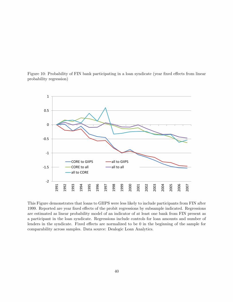
Figure 10: Probability of FIN bank participating in a loan syndicate (year fixed effects from linearprobability regression)

‐2

‐1.5

‐1

‐0.5

0

0.5

1

1991

1992

1993

1994

1995

1996

1997

1998

1999

2000

2001

2002

2003

2004

2005

2006

2007

CORE to GIIPS all to GIIPS

CORE to all all to all

all to CORE

This Figure demonstrates that loans to GIIPS were less likely to include participants from FIN after1999. Reported are year fixed effects of the probit regressions by subsample indicated. Regressionsare estimated as linear probability model of an indicator of at least one bank from FIN present asa participant in the loan syndicate. Regressions include controls for loan amounts and number oflenders in the syndicate. Fixed effects are normalized to be 0 in the beginning of the sample forcomparability across samples. Data source: Dealogic Loan Analytics.

40

Figure 11: Share of loans to GIIPS with at least one bank from FIN and CORE among mandatedlead arrangers

0

0.2

0.4

0.6

0.8

1

1990

1991

1992

1993

1994

1995

1996

1997

1998

1999

2000

2001

2002

2003

2004

2005

2006

2007

2008

2009

2010

2011

2012

As a share of total number of loans to GIIPS

at least one MLA from FIN

at least one MLA from CORE

This Figure demonstrates a decline in the share of loans to GIIPS that are arranged by FIN banksafter 1999 and a corresponding increase in loans to GIIPS that are arranged by CORE banks. Thesample is limited to loans to GIIPS. For each year the share of loans is computed (in terms of loancount), for which at least one of mandated lead arrangers is in FIN and in CORE. The remainingshare are loans for which none of the mandated lead arrangers are in FIN or CORE. Data source:Dealogic Loan Analytics.

41

Table 1: Cross Section regressions.

Dependent variable: ∆ln(BISC) ∆ln(BISL) ln∑

(BISLF) ∆ln(SLEC) ln∑

(LW)

2000-2007 1999-2007 1999-2007 1999-2007 1999-2007

(1) (2) (3) (4) (5)

CORE to FIN -0.605*** 0.0284 -0.818*** 0.296*** 3.709**

(0.148) (0.0673) (0.181) (0.0387) (1.359)

CORE to GIIPS 0.321** 0.722*** 1.715*** 0.311*** 1.289

(0.148) (0.0673) (0.169) (0.0387) (1.098)

FIN to CORE -0.0285 0.181** 0.851*** 0.674*** 3.817***

(0.148) (0.0673) (0.169) (0.0387) (1.220)

FIN to GIIPS 0.244 0.456*** 0.893*** -0.0285 -0.620

(0.148) (0.0673) (0.123) (0.0387) (1.076)

ln(Stock in 1999) 0.274*** 5.330***

(0.0420) (0.498)

Constant 0.821*** 0.659*** 0.558*** 0.175*** -0.979**

(0.148) (0.0673) (0.0485) (0.0387) (0.420)

Observations 556 1348 1760 1756 1140

Adjusted R2 0.019 0.0026 0.24 0.037 0.80

BISC is stock of total international bank claims from consolidated BIS data in real USD.

BISL is stock of total international bank claims from locational BIS data in real USD.

BISLF is valuation-adjusted flows of total international bank claims from locational BIS data in real USD.

SLEC is syndicated loan exposures as defined in the text aggregated on consolidated basis in real USD.

LW is the total amount of syndicated loans originated by country i to country j in year t in real USD.

Difference between logs of stocks in 2007 and 1999 or 2000 is computed for stock variables, as indicated.

Flows are summed up for years 1999-2007. We control for stock in 1999 for BISLF and LW flow regressions.

CORE includes Austria, Belgium, France, Germany, Netherlands, and Finland. GIIPS includes Greece,

Ireland, Italy, Portugal, and Spain. FIN includes Canada, Denmark, Japan, Sweden, Switzerland, the U.K., and the U.S.

ROW includes: Turkey, Taiwan, Hong Kong, and Singapore for BISC lenders, all 10 available

countries for BISC borrowers, all 31 available countries for BISL and BISLF lenders and borrowers.

The same 31 countries are included in SLEC and LW regressions for the ROW category.

Robust standard errors are clustered at lender region-borrower region pair level in parentheses.

*(P< 0.10), **(P< 0.05), ***(P< 0.01).

42

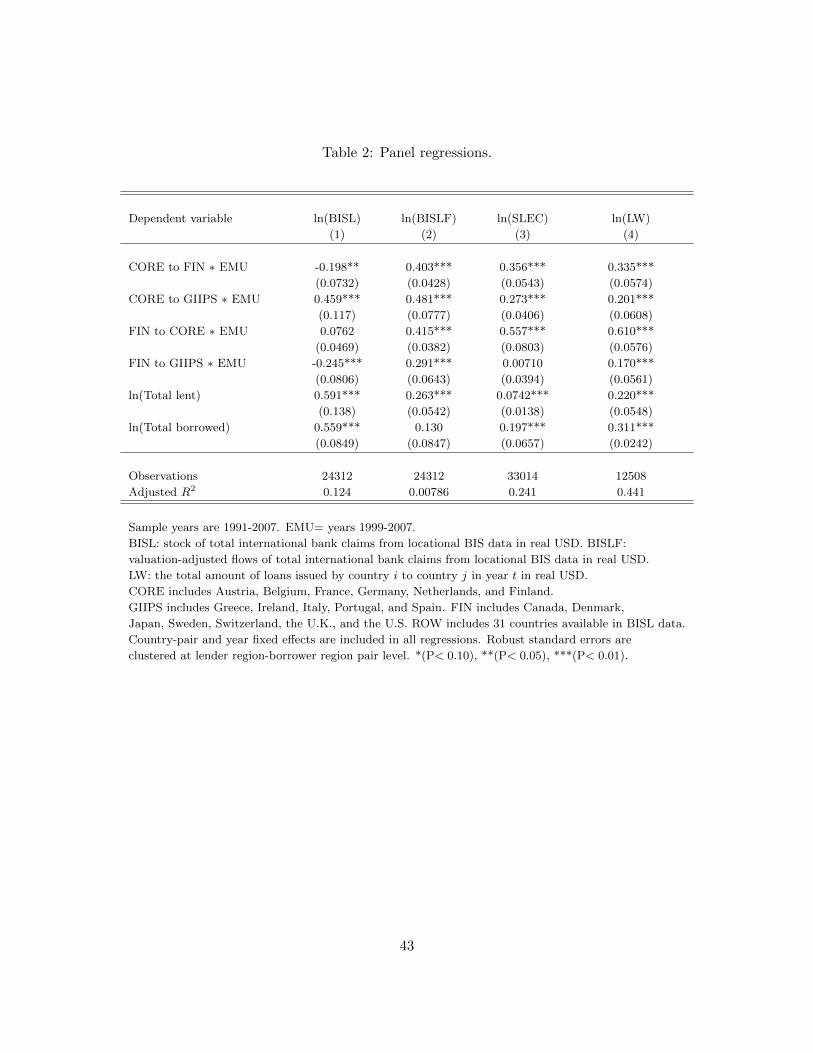
Table 2: Panel regressions.

Dependent variable ln(BISL) ln(BISLF) ln(SLEC) ln(LW)

(1) (2) (3) (4)

CORE to FIN ∗ EMU -0.198** 0.403*** 0.356*** 0.335***

(0.0732) (0.0428) (0.0543) (0.0574)

CORE to GIIPS ∗ EMU 0.459*** 0.481*** 0.273*** 0.201***

(0.117) (0.0777) (0.0406) (0.0608)

FIN to CORE ∗ EMU 0.0762 0.415*** 0.557*** 0.610***

(0.0469) (0.0382) (0.0803) (0.0576)

FIN to GIIPS ∗ EMU -0.245*** 0.291*** 0.00710 0.170***

(0.0806) (0.0643) (0.0394) (0.0561)

ln(Total lent) 0.591*** 0.263*** 0.0742*** 0.220***

(0.138) (0.0542) (0.0138) (0.0548)

ln(Total borrowed) 0.559*** 0.130 0.197*** 0.311***

(0.0849) (0.0847) (0.0657) (0.0242)

Observations 24312 24312 33014 12508

Adjusted R2 0.124 0.00786 0.241 0.441

Sample years are 1991-2007. EMU= years 1999-2007.

BISL: stock of total international bank claims from locational BIS data in real USD. BISLF:

valuation-adjusted flows of total international bank claims from locational BIS data in real USD.

LW: the total amount of loans issued by country i to country j in year t in real USD.

CORE includes Austria, Belgium, France, Germany, Netherlands, and Finland.

GIIPS includes Greece, Ireland, Italy, Portugal, and Spain. FIN includes Canada, Denmark,

Japan, Sweden, Switzerland, the U.K., and the U.S. ROW includes 31 countries available in BISL data.

Country-pair and year fixed effects are included in all regressions. Robust standard errors are

clustered at lender region-borrower region pair level. *(P< 0.10), **(P< 0.05), ***(P< 0.01).

43

Table 3: Total lending to GIIPS. Bank-level regressions.

Dependent variable Lent to GIIPS Lent to GIIPS Lent to GIIPS

Sample Bank in FIN Bank in CORE Bank in GIIPS

Borrowed from FIN * EMU -0.0480 1.134** 0.0372

(0.808) (0.517) (0.403)

Borrowed from ROW * EMU 2.182* 0.421 9.797**

(1.083) (2.898) (3.705)

Borrowed from CORE * EMU -0.581 -0.672** -2.109**

(1.651) (0.288) (0.944)

Borrowed from FIN 1.170 -3.524** -2.253

(2.910) (1.316) (1.921)

Borrowed from ROW 1.199 -5.060*** -2.074

(3.258) (1.129) (1.712)

Borrowed from CORE 1.847 -2.205 -1.863

(4.491) (1.446) (1.673)

Total lent by bank 0.085*** 0.064*** 0.069***

(0.0224) (0.0123) (0.00721)

Total borrowed by bank -1.163 2.329** 2.006

(3.245) (1.103) (1.717)

Observations 198 396 234

Adjusted R2 0.670 0.630 0.679

Sample years are 1990-2007. EMU= years 1999-2007.

Borrowed from X and lent to X are total amounts of loans issued by X in real USD.

CORE includes Austria, Belgium, France, Germany, Luxembourg (except CPIS), and Netherlands.

GIIPS includes Greece, Ireland, Italy, Portugal, and Spain.

FIN includes Canada, Denmark, Japan, Sweden, Switzerland, the U.K., and the U.S.

ROW includes Australia, China, Egypt, Hong Kong, Israel, Malaysia, Norway, Panama, Singapore,

Korea, Taiwan, Turkey, and Middle East and offshore financial centers.

Bank and year fixed effects in all regressions. Robust standard errors are in parentheses.

FIN banks: Barclays, Danske Bank, HSBC, Jyske Bank, Lloyds, Nordea Markets, Nykredit, RBS,

Svenska Handelsbanken, Swedbank First Securities, and Sydbank.

CORE banks: ABN Amro, Bayer, BNP Paribas, Commerzbank, Credit Agricole, Deutsche Bank, Dexia,

DZ Bank, Este Group, Helaba, HSH Norbank, Hypo, ING, KBC, Landesbank Berlin, Oesterrichische

Volksbanken, Op-pohjola, Rabobank, Raiffeisen, SNS Reaal, Weslb, and WGZ.

GIIPS banks: Allied Irish, Banco BPI, Banco Espirito Santo, Banco Popular Espanol, Bank of Ireland,

Bankia, BBVA, Caixa Geral de Depositos, Intesa Sanpaolo, Mote Dei Paschi, Santander, Unicredit, and UBI.

*(P< 0.10), **(P< 0.05), ***(P< 0.01).

44