Embed Size (px)
Citation preview

The Equivalent Single Scenario in an Arbitrage Free
Stochastic Interest Rate Model
Author: B. John Manistre PhD FSA FCIA MAAA Crown Life Insurance Co. P.O. Box 827, 1901 Scarth St., Regina, Sask., S4P 3B1 Canada. (306) 751-6178, Fax (306) 751-6219
Abstract This paper explores a formal mathematical relationship between arbitrage free option pricing methods and traditional actuarial discounting. Whenever contract persistency is interest scenario dependent it is shown how an option pricing approach can be modified to derive a single set of interest, decrement and other assumptions such that discounting along this single scenario using traditional actuarial techniques will produce the same present value as the option pricing model.
The main result is that the derived interest and persistency assumptions contain margins which reflect the costs of the embedded options. When no options are utilized then the equivalent single interest rate scenario is simply the set of forward rates implied by the starting yield curve. When options are present the option adjusted forward rates nay be above or below the starting rates depending on how contract persistency is related to interest rate movements. The sign of the margins produced by this method is in accord with common sense reasoning.
An example is given of a traditional, fixed cash value, insurance product subject to interest sensitive withdrawal and inflation driven expenses. By using idealized interest rate and surrender assumptions it is possible to use calculus, rather than numerical calculation, to do the option pricing mathematics and produce a set of simple formulae for the equivalent single scenario interest, mortality, withdrawal and expense assumptions.
The paper continues by extending the concepts to interest sensitive products such as Universal Life and the SPDA. Formulae for single scenario account values, credited rates, surrender charges and other variables are developed. In addition, non-zero covariances between some of the interest sensitive variables lead to new terms which have no analog in the traditional actuarial approach.
The discussion of interest sensitive products is concluded by presenting the results from a moderately realistic numerical study of an SPDA.
The paper concludes with a brief overview of applications of the single scenario idea in the current environment.
1079
Le scenario unique Bquivalent dans un modMe de taux d’intMt stochastique
sans arbitrage
B. John Manistre Phd Fsa FCIA MAAA Crown Life Insurance Co.
P.O. Box 827, 1901 Scarth St., Regina, Sask., S4P 3Bl
Canada (306) 751-6178, Telecopie (306) 751-6219
R&urn6
La presente etude examine les relations mathematiques formelles qui existent entre les methodes d’bvaluation des options sans arbitrage et I’actualisation actuarielle traditionnelle. Chaque fois que la persistance du contrat depend de l’evolution du taux d’interbt, nous indiquons ici comment la methode d’evaluation de I’option peut btre modifiee pour obtenir un ensemble unique d’interet, de decrement et autres parametres tels que I’actualisation effect&e au moyen de ce scenario unique par les techniques actuarielles traditionnelles produisent la mgme valeur actuelle que le mod&e d’evaluation des options.
Le principal resultat est que les hypotheses relatives B I’interbt et g la persistance prevoient des marges qui refletent les co&s des options incluses. Lorsque I’on n’utilise pas d’options, le scenario de taux d’interbt unique equivalent est simplement I’ensemble des taux futurs donnes par la courbe des rendements initiaux. Lorsque des options sont presentes, les taux futurs ajustes par les options peuvent &re superieurs ou inferieurs aux taux d’int&Qt initiaux, selon les relations qui existent entre la persistance du contrat et l’evolution des taux d’interbt. Le sens des marges produites par cette methode est conforme au raisonnement logiqua
Nous donnons ici I’exemple d’un produit d’assurance traditionnel ZI valeur de rachat fixe soumis B des retraits sensibles aux taux d’interet et I des charges resultant de I’inflation. En utilisant un taux d’interbt idealise et des hypotheses de rachat, il est possible de proceder B des calculs differentiels plut& que simplement numeriques pour proceder a I’evaluation de I’option et pour produire un ensemble de formules simples en rendant compte des hypotheses de scenario unique equivalent pour I’interet, la mortalite, les retraits et les charges.
Nous poursuivons notre analyse en Btendant ces concepts aux produits sensibles aux taux d’interbt, tels que les contrats vie universels et les contrats g prime unique B prestations differees (SPDA). Les formules de scenario unique pour les valeurs de comptes, les taux credit&, les charges de rachat et autres variables sont developpees. En outre, les covariances non-zero entre certaines des variables sensibles aux taux d’interbt menent B definir de nouveaux termes qui n’ont pas d’analogues dans la methode actuarielle traditionnelle
Dans le cadre de I’examen des produits sensibles aux taux d’interet, nous presentons Bgalement les resultats d’une etude numerique moderement realiste d’un contrat SPDA.
Le present article donne pour conclure un bref apercu general des applications du concept du scenario unique dans le contexte conjoncturel actuel.
1080

ARBITRAGE FREE STOCHASTIC INTEREST RATE MODEL 1081
Introduction
This paper explores a formal mathematical relationship between arbitrage free option pricing methods and traditional actuarial discounting. Whenever contract persistency is interest scenario dependent it is shown how an option pricing approach can be modified to derive a single set of interest, decrement and other assumptions such that discounting along this single scenario using traditional actuarial techniques will produce the same present value as the option pricing model.
The main result is that the derived interest and persistency assumptions contain margins which reflect the costs of the embedded options. When no options are utilized then the equivalent single interest rate scenario is simply the set of forward rates implied by the starting yield curve. When options are present the option adjusted forward rates may be above or below the starting rates depending on how contract persistency is related to interest rate movements. The sign of the margins produced by this method is in accord with common sense reasoning.
A simple, intuitive, overview of the author's result can be developed by breaking down the option pricing approach' into the following four steps
a) Develop an arbitrage free set of interest rate paths
s .
b) Project the contract's cash flows along each scenario to
get a matrix of cash flows CFZ where t is time and CL
indexes the scenarios.
cl Discount the projected cash flows using the sequence of 1 period interest rates associated with each scenario.
d) Average the present values obtained in step (c).
Symbolically this can be written as
Where N is the number of scenarios and v: discounts for
interest.
Relative to the development above the single scenario approach can

4TH AFIR INTERNATIONAL COLLOQUIUM
be described as replacing the last two steps above with the following,
1) Reverse the order of summation in the equation above to 9-t
v=c f-O ( $2 v: CF:)
2) Carry out the sum over scenarios and reorganize so as to make the result look like a standard present value calculation.
v = c 0, c?, t-0
Whenever contract persistency varies by scenario the algebraic process of summarizing many scenarios into one i.e.
can be done in a way which is essentially unique. This will be shown in detail later.
The remainder of this paper is organized into four sections as follows.
1) Following this introduction is a section dealing with a traditional fixed cash value, insurance product subject to interest sengitive withdrawals and inflation driven expenses. This simple model is used to develop the main principles used to average many scenaios into one. An example is given that uses interest rate, inflation and surrender assumptions which are simple enough that it is possible to use calculus, rather than numerical calculation, to do the option pricing mathematics and produce a set of simple formulae for the equivalent single scenario assumptions of interest, withdrawal and expense.
2) The next section extends the theoretical results described above to interest sensitive products such as Universal Life and the SPDA. When the ESS method is applied to interest sensitive products some new terms emerge which have no analog in the deterministic model.
In order take advantage of the stochastic calculus as a theoretical too1 all models in sections 1 and 2 use continuous time mathematics.
3) The third section of the paper reports the results of a

ARBITRAGE FREE STOCHASTIC INTEREST RATE MODEL 1083
numerical study of an SPDA. There are three subsections. The section opens with a discrete time formulation of the main results of section 2. The second subsection outlines the detailed assumptions that must be made for various quantities such as interest rate volatility, interest sensitive withdrawals and rate crediting strategies. The final part of section 3 summarizes the numerical results and discusses some of the calculated 'Equivalent Single Scenario' quantities.
4) The fourth and final section of the paper briefly discusses applications of the ESS technique.
Section l-Traditional Individual Insurance Products
In this section we consider a model of a traditional non- participating individual whole life insurance contract with fixed
death benefit and surrender value schedules DE, , CV, .
It will be assumed that the force of withdrawal at time s, p: ,’
is a random variable which varies by scenario in a way which reflects the assumed behaviour of the policyholder. Similarly, the
force of mortality pz might vary by scenario if healthy lives are
more apt to exercise their surrender options than are unhealthy lives.
Finally, let e(s) and g(s) denote random variables for expenses and gross premiums per unit inforce. Some unit expenses will vary with inflation while others may vary depending on the number of policies remaining inforce. In either case expenses will vary by scenario. The gross premiums may vary by scenario if the product is
adjustable. If not then g(s) is simply a scalar(non random) quantity.
With these definitions we can use the basic option pricing process the write the value of the contract as an expected present value
V(t) =E,jco [p~DE,+p~CV,+e(s) -g(s)]& (1.1) t
Where
' All random var ibles w ill appear in bold typeface.

1084 4TH AFIR INTERNATIONAL COLLOQUIUM
G(s) = exp-jh(s) +P:+p:l ds, f
discounts for interest and persistency* along each scenario, r(s)
is the instantaneous force of interest, and E, is the risk
neutral expectation operator given data up to time t.
We now begin the process of taking the expectation operator inside the integral. This amounts to averaging over the scenarios first.
Start by looking at the expected discount factor symbolized by
e(s) = E,[G(s)l skt. (1.2)
Differentiating this expression we find
-$6 =lim E,(G(s+As) -G(S))
AS-O As
= -EdG(r+ p"+ ~91
If we now define the Equivalent Single Scenario (ESS) forces of interest and decrement by
8(s) = E, [G(s)r(s) 1 E(s) ’
a” Ps = E, [G(s) p:l
E(s) ’ (1.3)
Then it follows that
* The symbol G is used here rather than the traditional actuarial symbol tEx for an endowment in order to avoid confusion with the symbol for the expectation operator. The symbol G is also more standard in the finance literture.

ARBITRAGE FREE STOCHASTIC INTEREST RATE MODEL 1085
and therefore
i.e. the ESS rates of interest and decrement are those which produce the expected discount factor. The definitions in (1.3) are the key ideas needed to reduce many scenarios into one.
If we interchange the operations of integration and expectation in the definition of V(t) we can put the ESS quantities back into V(t) to get
s+p;cvs+&(s) -g(s) Ids.
Where
&(s) = E,[G(s)~(~) 1
E(s) ’
9(s) = E,[G(s) g(s) I
c?.(s) ’
(1.4)
(1.5)
are the ESS expense and premium assumptions.
The structure of (1.4) shows that the option valuation problem has been reduced to a traditional actuarial present value calculation using a single set of interest, decrement, expense and premium assumptions. The descriptive term 'Equivalent Single Scenario' is therefore appropriate.
As can be seen from equations (1.3) and (1.5) the reduction from many to one scenario is achieved by an averaging process which
replaces a random quantity X(S) with
B(s) = E,[x(s) G(s) 1 E,G(s) ’
= X(s) + Cov[X(s) ,G(s) I . E,G(s)
(1.6)

1086 4TH AFIR INTERNATIONAL COLLOQUIUM
For the remainder of this paper we will refer to an average of the
form (1.6) as the ESS value and use the notation 2 for this average. The only exception to this notation will be the
definition of 6 given in (1.2).
The formal analogy with traditional actuarial mathematics can be
taken a step further. If V(S) denotes the value of the contract
at a future time s >t then we can define a new quantity Q(s) by
O(s) = E,[G(s) V(S) 1 G(s)
(1.7)
Then it is easy to show that O(s) satisfies the following classical differential equation for the time evolution of a reserve
dQ = (8(s) ds
+p:+p:, O(S)
- [fi: CV, + (i; DE, + e^(s) - g(s)]. (1.8)
Given the close formal analogy between classical actuarial mathematics and the ESS quantities it might appear that there is nothing new in this approach. What is new is that the ESS approach yields insight into what kind of biases should be put into deterministic assumptions in order to take account of stochastic cash flows.
As an example we consider how the ESS forward rates
8s reflect the impact of interest sensitive decrements. To do
this we rewrite the discount factor as the product of separate interest and persistency factors
G(s) = v(s) p(s),
where s
v(s) = exp- /
r(s)ds, p(s) = exp-jtp: + &ds. e f
Then we can rewrite (1.3) as Now consider what happens when the forces of decrement are not

ARBITRAGE FREE STOCHASTIC INTEREST RATE MODEL 1087
8(s) = E,[r(s)v(s)p(s)l E,[v(s)p(s) 1 \
(1.9)
interest sensitive ie. they are simple deterministic functions of time alone. Then equation (1.9) simplifies to
B,(s) = E,[r(s)v(s)l
E,v(s) (1.10)
Here gf(s) is the force of interest to be used to discount cash
flows which do not vary by interest rate scenario. In most
practical interest rate scenario generators b,(s) is the set of
forward rates built into the starting yield curve.
BY comparing equations (1.9) and (1.10) it is possible to understand, in a qualitative way, how the option adjusted forward
rates b(s) differ from the fixed cash flow forward rates b,(s) .
Both quantities are present value weighted averages of the short
term rate r(s) .
Suppose that high option election rates cl: are associated with
high interest rates as would be the case with a typical life insurance policy. Then high interest rate values will be associated with lower persistency values p(s) and will receive a lower relative weighting in (1.9) than they would in (1.10) i.e.
8(s) i b,(s) .
In a model of a callable bond high option election rates would be associated with lower interest rates so the opposite conclusion
would hold i.e. S(s) 2 a,(s) .
The above argument suggests that the ESS interest rates derived from this process are in accord with common sense intuition in that the bias will be in the appropriate direction.
We close this section with an example to illustrate the theoretical

4TH AFIR INTERNATIONAL COLLOQUIUM
concepts discussed above. For the interest rate model we take Vasicekrs2 (1977) interest rate model. In this model the short term
spot rate r is the only state variable and is assumed to follow the risk neutral stochastic process
dr = [a(0 - r) + qaldt + adz.
For this model it is known that the forward rates at time s, given
r(t)=r , are
&,(s) = r .-a(s-t) + (e+T) (l-e-“(S-t)) - $[(1-e-“(s-t))/a]2.
We will combine this model of interest rates with
an interest sensitive withdrawal p: = p," + EK , which is linear in
stochastic interest rate.
Unit expenses will be assumed to inflate at the short term rate less a fixed margin A , i.e. we assume the expense random variable is given by
e(s) = e(t) expj(r - Adds. f
We will assume all other quantities such as mortality and premium payments are deterministic.
The results for the ESS interest, withdrawal and expense assumptions can be shown to be
6 = 6 f cu2 l-eeas 2
5 2 ( - 1 I a
and

ARBITRAGE FREE STOCHASTIC INTEREST RATE MODEL 1089
If E>O (eg. life insurance ) then the ESS interest rates are
lower than the forward rates. If E<O then the ESS rates are higher than the forward rates. This result is in accord with arguments presented earlier.
Looking at the expression for the ESS expenses we recognize the expression under the integral sign as an effective inflation rate. The first two terms inside the integral above are no surprise being the ESS forward rates less the margin. The third term shows that
with ~20 persistency an even greater impact on inflation than it does on interest rates. This makes some sense in that higher lapse rates will lead to lower expenses. The example does not consider the effect fixed expenses would have.
The example above is not intended to be realistic. It merely illustrates the kind of relationships that would exist in a more complex model that will have to attacked using computers instead of calculus.
For a more details on the derivation of the formulae related to this example see Manistre 3

1090 4TH AFIR INTERNATIONAL COLLOQUIUM
Section 2 - Interest Sensitive Products
This section extends the ESS theory developed for traditional products to interest sensitive products. Mathematically, the interest sensitive product differs from the traditional products in that we will have to consider products of random variables eg. the product of an account value and a credited rate or surrender charge. This means that we not only have to consider mean values of the form
i(s) = E,[G(s)X(d 1 G(s)
but also covariances of the form
C&(X, Y) = E,[G(s)X(s) Y(s) 1 _ 2p e(s)
More complex situations can easily arise when considering real products.
We start by considering a valuation problem of the form
4 7
v(t) = E /G(s) LP: DB, + p1~C.s) Cl-SC,)+e(s)-g(s)lds + V(T)G(T) t
(2.1)
All symbols previously defined retain their meaning. The new symbols appearing in (2.1) are the account value R(s) and the surrender charge SC. Bold typeface for the death benefit symbol DB indicates that we now allow it to vary by scenario as would be necessary to model Universal Life.
The formula above assumes that the net surrender value is the account value reduced by a scale of surrender charges. This scale may be deterministic (eg. a fixed scaled grading from 7% down to 0% over 7 years) or stochastic (eg. an SPDA with a bailout provision).
The account value is assumed to evolve according to a stochastic process of the form
dR(s) = [c(s)R(s)-p,(DE,-R(s))-B,+g(s)]ds. (2.2)
Where c(s) is the instantaneous credited rate, p, is the cost
of insurance rate charged to the account value and C, is the

ARBITRAGE FREE STOCHASTIC INTEREST RATE MODEL 1091
expense charge rate. As before g(s) is the gross premium.
Using the definitions
Q(s) = E, [G(S) V(s) 1 /G(s) I?(S) =E,[G(s)R(s) I/~(S)
we can rewrite equation (2.1) as T
o(t) = /8(s) r~~&,+~:R(s) (l-SYJ +d(s) -4(s) 1 ds f
+ TB(s) [&v(DEJ, pd) +&v(R, p") Ids + O(T) e(r) I
(2.3)
I c
Where
s-Ps = E, [sc,d R(s) G(s) I p; l?(s) E(s) ’
will be known as the Effective Surrender Charge rate.
Equation (2.3) introduces two new issues. Firstly, the terms
C%&R(s) ),Cb'(&DB,) which appear in (2.3) have no analog in
traditional actuarial mathematics. Secondly, in order to get a single scenario scale of surrender charges we have had to use a new
kind of averaging process. The symbol ST has been used rather
than S^c to highlight this fact. We will also use the term Effective Surrender Charge rather than ESS Surrender Charge.
We now look at the evolution of the quantities i(s), Q(s) to see if they behave like their deterministic analogues. This will then lead to a representation of V(t) as the account value R(t) less a present value of future margins. Where possible, definitions are made to allow the resulting relationships to mimic the deterministic theory as much as possible.
Start with the definition of ESS account values
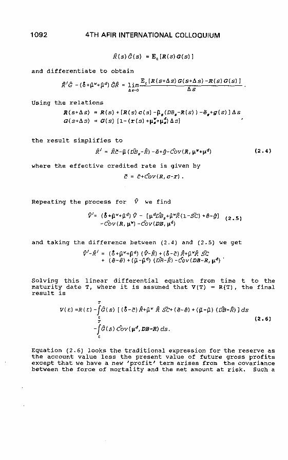
1092 4TH AFIR INTERNATIONAL COLLOQUIUM
J?(S) E(S) = E, [R(S) G(S) 1
and differentiate to obtain
iv8 - (b+@“+Fd) &? = I;;-; E,[R(s+Ass)G(s+As)-R(s)G(s)]
As
Using the relations R(s+As) = R(s)+[R(s)c(s)-&(DB,-R(S))-S,+g(s)] As G(s+As) = G(s) [l-(r(s)+p:+& As]
I
the result simplifies to
i?’ = &Z-p (&,-I?) -Z+@-&v(R, p”+pd)
where the effective credited rate is given by
E = C+&v(R,c-r).
(2.4)
Repeating the process for P we find
Q’= (6+fi”+fid, Q - [pdD~,+pwl?(l-s^c) +&-@I (2*5) -&v(R,~")-&v(DB,~~)
and taking the difference between (2.4) and (2.5) we get
Q'-RI' = (i$+pw+@d) (9-j) +(n$-p)R^+py+ s'c + (&&)+(ji-fid) (D%-R")-&v(DB-R,~~)
Solving this linear differential equation from time t to the maturity date T, where it is assumed that V(T) = R(T), the final result is
V(C) =R(t) -j&s) [(8-E)lT+PWl? .s’c+(&-Is) + (p-p, (&3-l?) 1 ds it T (2.6)
~(s)&~v(~~,DB-R)ds. t
Equation (2.6) looks the traditional expression for the reserve as the account value less the present value of future gross profits except that we have a new 'profit J term arises from the covariance between the force of mortality and the net amount at risk. Such a

ARBITRAGE FREE STOCHASTIC INTEREST RATE MODEL 1093
term might contribute to the valuation if one assumed that there was interest rate driven selective lapsation.
Equation (2.6) also has all of the traditional sources of revenue. Note that in the spread term the ESS force of interest plays the role of the earned rate. Other sources of revenue in (2.3) are surrender charges, the difference between expense loadings and expenses incurred and the loadings available in the cost of insurance charges.
This completes the development of the mathematics underlying the Equivalent Single Scenario concept. While the details of calculating the ESS can be complex there is one underlying simple principle viz. the idea of using present value weighted averages, where the present values discount for both interest and persistency. Since actuaries use the term 'Endowment factor' to refer to a quantity which discounts for both interest and persistency the ESS quantities could also be called 'endowment weighted averages'. While there are some exceptions to rule of using endowment weighted averages it is clear that the resulting theory is formally very close to traditional actuarial discounting.
It is natural to ask whether these ideas have any practical value. This issue will be discussed after a more practical example of an ESS calculation has been presented.
Section 3 - Numerical Study of an SPDA
In this section we present an ESS analysis of a Single Premium Deferred Annuity contract (SPDA) as that tern is currently understood in the United States' individual insurance marketplace.
An overview of the process involved is as follows,
1) An arbitrage free set of interest rate paths was generated from an assumed initial yield curve and a set of volatility assumptions for each point on the curve together with assumed correlations between different parts of the yield curve .
2) Cash flows for policy benefits and expenses were developed for each scenario using assumptions for rate crediting by the insurer, competitor interest rates, surrender charges & bailout features, expenses, mortality and policyholder lapse behaviour.
3) The cash flows and discount factors developed in steps (1) and (2) above were summarized into one scenario using the principles developed earlier in this paper.
4) The results of the ESS analysis will be discussed.

4TH AFIR INTERNATIONAL COLLOQUIUM
For the benefit of readers who may have skipped the theoretical sections of this paper we briefly review the principles used to average many scenarios into one. This review will also deal with some of the additional details that arise when going from continuous time to discrete time. There are no new principles.
a) The primary principle is that most quantities that vary by scenario are replaced by their 'endowment weighted average'.
If G; is the endowment factor at time t on scenario a i.e.
G= C+l = G; v: (1-q: -w:, , (3.1)
then most quantities such as expenses, premiums and account values are replaced by an average of the form
(3.2)
In equation (3.1) v," is the one period risk free discount
factor for that time period and scenario, qt is the
corresspondinq probability of death and W," is the
probability of surrender.
There are exceptions to the rule outlined above. In particular
we will use the symbol 6, for the average endowment factor
(3.3)
The most important exceptions will be for credited rates and surrender charges. All of these exceptions arise from the need to consider sums of the form
involving products of three or more variables that vary by scenario.

ARBITRAGE FREE STOCHASTIC INTEREST RATE MODEL 1095
As an application of the general rule consider the ESS interest rate and decrement factors which are given by
c G: v: v,= a
N& ' c G: vc" s:
4t= = N&V, '
c G; v; wt" 8,= a
N&v, '
(3.4)
With these defintions the average endowment factor satisfies
e,*, = e,v,c1 -4, -8,) * (3.5)
The defintions of the ESS mortality and withdrawal in (3.4) might seem to violate the averaging rule (3.1). However, further consideration shows that these quantities are still 'endowment weighted averages' provided one assumes that all deaths and withdrawals take place at the end of time periods. The ESS averages are therefore calculated the instant just before people die or surrender which is consistent with (3.5).
Other timing assumptions are possible and will produce different results from what is reported here. These are details which do not have to be considered in the continuous time models presented earlier. However, once a set of timing decisions is made the principles for ESS aveaging can always be applied in a reasonable, if not always unique, way.
As a further example note that if the one period interest rate it”
is related to the discount factor via v: = l/(l+it) and if
then it follows that
v, = l/(1+1",) *
In this case we see that the interest earned needs to be placed at the end of the time period wheras the discount factor belongs at

4TH AFIR INTERNATIONAL COLLOQUIUM
the beginning of the period. Both of results make intuitive sense.
The table following this page is a one page summary of assumptions and results for the SPDA study.
The first part of the table outlines the assumptions used to generate cash flows along each scenario. These assumptions are for illustration only. The author does endorse any particular assumption used in this paper.
The product is an SPDA with the credited rate reset by the insurer once each year. The insurer is assumed to set the rate at the then current 1 year Treasury rate. It is assumed that there is always a competitor somewhere willing to offer the 5 year rate on a product that the policyholder would consider to be a substitute to his current contract.
A bailout feature has been added to the contract in order to study its effect on the ESS surrender charges. If the insurer ever resets the rate below the initial credited rate then the policyholder has 3/S of a year to surrender the policy for its full account value.
Interest rate driven surrenders are assumed to occur at the annual rate given by the formula in the table. This formula was inspired by examples given in New York's Regulation 126. After 10 years all remaining policies are assumed to surrender.
This rather simple product was chosen because it is relatively easy to tell if the results produced by the analytical machinery are reasonable.

ARBITRAGE FREE STOCHASTIC INTEREST RATE MODEL 1097
Summary of Assumptions and Results
Number of Scenarios 1,000
1 o/05/93 lo:20 PM
ASSUMPTIONS Plan Type Rate Crediting Competitor Rate Surr Charges Bailout Feature Expenses Average Size Inflation Mortality Lapse Formula
SPDA lyr Guarantee Periods 1 yr Treasury coupon rate 5 yr Treasury rate spot rate 7,6,5,4,3,2,1 unless bailout window open 135 day window 0 bp below initial rate 5% of Prem + (65O/pol +$&IO/decrement) inflated 25,000 1 yr rate less 250 bp 65-70 Ult male age 55 at issue 150+max(.25%,(Cred %-Competitor)) * 2 + 8% - Surr Chg %
interest Rates - Log Normal parametres
Volatilities 1.5 mths.
20.00% 3 mths. 19.95%
Correlations Corr to Short Corr to 3 mth Corr to 1 Yr Corr to 5 Yr Corr to 10 yr Corr to 20 yr
Initial Spot % Initial Forward %
RESULTS ESS Initial Spot % ESS Initial Fwd % ESS Opt Adj Spot % ESS Opt Adj Fwd % ESS Cred % ESS Inflation
Reserve at Issue PV Gross Surr. Ben PV Surr Charges PV Dth. Ben PV Expense PV Prem. Unreconiled Total
1 yr 19.65%
W 18.03%
10yr 16.00%
20 yr 12.00%
100.0% 99.9% 99.1% 95.1% 90.0% 85.0%
99.9% 100.0%
99.7% 96.4% 91.7% 85.1%
99.1% 99.7%
100.0% 98.2% 94.4% 85.4%
95.1% 96.4% 98.2%
100.0% 98.8% 87.5%
90.0% 91.7% 94.4% 98.8%
100.0% 90.0%
85.0% 85.1% 854% 87.5% 90.0%
100.0%
3.25% 3.25%
3.29% 3.32%
5.00% 6.90%
6.50% 9.04%
7.50% 7.97%
3.25% 3.25% 3.25% 3.25% 3.44% 1 .cO%
3.28% 3.31% 3.28% 3.31% 3.44% 1.07%
3.50% 3.75%
3.50% 3.75% 3.49% 3.73% 3.44% 1.56%
5.01% 6.86% 4.88% 6.49% 6.05% 3.89%
6.47% 8.85% 6.03% 7.80% 7.28% 4.74%
924.23 (19.31) 65.18 81.29
(1,000.0) (0.01)
Present Value of Revenues Surr Charges 19.31 Spread 10.58 Mort Gain 0.00 Expense Cov(q,NAR)
W.3
Unreconiled 0.01 51.38 +-0.65 (51.38)+ -0.65
bp Required Spread over Treasuries Option Adj. Duration OAS Duration
85 1.65 yrs. 5.95 yrs.

1098 4TH AFIR INTERNATIONAL COLLOQUIUM
The next part of the summary documents the assumptions used to generate the interest rate scenarios. Any reasonable method of scenario generation can be used for an ESS analysis. The actual
approach used here was to assume that spot rates xi at all points
of the form iAt along the yield curve follow a lognormal
distribution. That is if, exp( -ixiAtt) is the value at time
sAt of a cash flow due iA t later, then the yield curve at time s+l is related to the curve at time s by
f i*l XS
i*lmX1
x=+1 = x, +d + -$i (x,'J2piiAt2 + ~x,'pfz"JhE. (3.6) 1 E-1
Here the za represent 3 independent normal deviates and pf is
a matrix designed to generate the desired correlations and
Equation (3.6) is an expression of the requirement that
e-fj+l)x!-'At = e-~:~ .-jxLIAf (3.7) s
under the assumption that the time step is small enough that that
the lognormal variables j x,*1 can be approximated by normal
variates.
The method is arbitrage free in the sense that (3.7) holds and it implies
A random sample of scenarios will therefore reproduce the starting yield curve to within sampling error.
In the limit as the time step At goes to 0 and the scenario sample gets large most theoretical problems with this approach go away. In this limit the method used here would agree with the approach described by Miller 4.

ARBITRAGE FREE STOCHASTIC INTEREST RATE MODEL 1099
From a practical perspective the advantages of this approach are its ease of implementation and the fact that it puts no restriction on the starting yield curve'. Disadvantages of this approach are the amount of computation required and, with a finite time step, there is always the possibility of a negative spot rate appearing in one or more scenarios. There is also the issue of sampling error.
For the current application the ease of implementation was an important consideration because it allowed all of the calculations reported here to be carried out in an electronic spreadsheet.
In this paper a time step of 1/8'th of a year was used with the initial spot rates shown in the summary table. Linear interpolation of the forward rates was used to get intermediate values. Correlations and volatilitiies were specified at durations l/8, 10 years and 20 years with interpolation in between.
Note that due to the relation (3.6) all 20 years of yield curve data could affect the analysis even though it is assumed that policy is surrendered after 10 years.
For a more thorough discussion of scenario eneration methods see the previously referenced article by ? Tilley .
With this backround we can now discuss the results of the analysis.
The first two lines in the results section report the initial fixed cash flow spot rates and forward rates as calculated from the scenario set. The difference between these values and the intial rates used to seed the scenario generator are an indication of the sampling error in the model. For example the 10 year spot rates differ by 3 bp. The forward rates differ by 19 bp.
The next set of results shows the option adjusted ESS rates along with the ESS credited rates and ESS inflation rates. A more complete presentation of these values over the 10 year study period can be found in the graph labelled 'ESS INTEREST RATES'.
The results confirm the theory devloped in section 1 of this paper which showed that the ESS forward rates should be lower than the fixed cash flow rates when lapses are positively correlated with higher interest rates.
3Discontinuities in the forward rates or any of its derivatives can cause practical problems.

10.00%
9.00%
S.OO%
7.00%
g 6.00%
2
z 5-oo% “J s 4.00%
3.00%
200%
1.00%
0.00%
ESS Interest Rates 1000 Scenarios RSA = S5 bn
-
-
-
-
-
- J -
-
d;
v 1 z 3 4 5 G 7 s 9 10 Time in Years
-+ ESS Initial Fwd % + ESS Opt. Adj. Fwd % 10/S/93 PVFB = 1051.35+ -0.65
+ ESS Cred % + ESS Inflation %

ARBITRAGE FREE STOCHASTIC INTEREST RATE MODEL 1101
The ESS credited rates follow the ESS forward rates quite closely indicating that the insurer is earning very little spread by crediting the 1 year Treasury rate. What spread is available seems to be function of the slope of the yield curve.
The ESS inflation rates are roughly paralell to the option adjusted forward rates as expected. The impact of sampling error is quite evident in the small fluctuations of this curve.
At the bottom of the results page we see two decompositions of the reserve at issue. The two presentations are derived from discrete time analogs of equations (2.3) and (2.6). The reserve is $51.58 just prior to a $1,000 deposit. This indicates that the 5% commission cost is never recovered.
At the bottom of the summary table is reported the option adjusted duration and the Required Spread on Assets. The option adjusted duration is a measure of the sensitivity of the final result to a paralell shock in the yield curve taking place just after the initial credited rate is set. The SPDA has the same price sensitivity as a 0 coupon bond with a maturity of 1.65 years.
According to option pricing theory the insurer should invest the initial reserve, net of commissions, in a portfolio of treasury bonds with that same price sensitivity. See Norris and Epstein' for a numerical demonstration of this theory.
One way to overcome the loss indicated above is to assume that the insurer can invest in assets which have the same characteristics as a matching portfolio of Treasury bonds except that they earn an additional 85 basis points. The sensitivity of the value to a change in this margin is known as the OAS duration which is reported as 5.95 years, i.e. 85 basis points over roughly 6 years will recover the lost commissions. It can be shown that the OAS duration is equal to the Macaulay duration of the ESS cash flows discounted along the ESS option adjusted yield curve.
Finally we discuss the ESS lapse rates and surrender charge rates. These values do not appear in the summary table due the amount of data involved. The two quantities are shown on a graph tilted 'ESS Lapse Rates and Surrender Charges'.
The Effective Surrender Charges were calculated using a discrete time analog of equation (2.4). The bailout window was assumed to open for the first 3 time periods of each year. Therefore on some scenarios the bailout was broken and some not. If the bailout was broken then the surrender charge drops to 0 and additional surrenders take place according the lapse formula. The impact of this behaviour is to reduce the effective surrender charge during the first part of each policy year as shown.

1102 4TH AFIR INTERNATIONAL COLLOQUIUM

ARBITRAGE FREE STOCHASTIC INTEREST RATE MODEL 1103
The ESS surrender rates proved to be very sensitive to sampling error. Reasonable estimates of the present value and option adjusted duration can be obtained with a modest (about 25) number of scenarios. However, calculating ESS quantities with any precision can require a much large number of scenarios. Even with 1000 scenarios there is still a visible amount of statistical noise in the result. With more scenarios (about 5,000) the lapse rates within a policy year follow a smoothe pattern with a minimum at the begining, just after the rate has been reset, rising steeply during the year as opportunities for higher competitor rates present themselves. The overall pattern follows the runoff of surrender charges.
In general the more volatile the cash flows are the more scenarios will be required to get smoothe results. More scenarios are also required as the analysis goes further out in time.
This concludes the discussion of this particular example.

1104 4TH AFIR INTERNATIONAL COLLOQUIUM
Section 4 - Applications of the ESS Concept
The ideas of this paper were developed with two goals in mind. These were to
1) Increase understanding of the option pricing method and it's implications and,
2) Help develop actuarial assumptions for traditional actuarial applications such as pricing and financial reporting.
One immediate application within option pricing is the result stated earlier that the Macaulay duration of the ESS cash flows is equal to the OAS duration of the financial instrument.
Another application is that ESS concepts make it clear why the Option Adjusted Duration can be so different from the OAS duration. The basic answer is that when the yield curve changes so do the ESS cash flows. After having seen a number of examples it is possible to develop intuition and insight into price sensitivities based on ESS concepts.
An organization that wants to do option pricing valuations on its assets or liabilites may find the ESS approach a practical way to make use of traditional GAAP or PPM oriented valuation systems to do the valuation. A subsystem could be developed to do the ESS analysis and produce assumptions that are then installed into the main valuation system. This would be more useful for traditional insurance products than it would be for interest sensitive products.
Another potential application within option pricing itself is to try to improve the precision of valuation models by calculating the ESS cash flows and then smoothing or graduating them to remove noise. In some cases this may be a more efficient use of computational resources than calculating additional scenarios.
While option pricing should have a role in pricing its role in financial reporting is not so clear. Actuaries performing GAAP valuations in the United States or PPM valuations in Canada must choose assumptions which are prospective in all respects save one. In both countries the actuary is forced to develop an interest rate assumption which allows the resulting liabilities to make sense when compared to assets which, by and large, are valued retrospectively. This fact tends to force financial actuaries to look to other tools, such as cash flow testing, for dealing with investment related issues.
However, option pricing does capture certain economic realities and these could be recognized in the following example. Suppose a valuation actuary has developed an interest assumption for a block

ARBITRAGE FREE STOCHASTIC INTEREST RATE MODEL 1105
of policies without options and backed by a known portfolio of assets. He now considers valuing a block of similar policies, backed by the same asset pool, but containing options. How should he bias the assumptions to take account of the options? One answer is to use the biases produced by an ESS analysis of the policies with options. This position would be reasonable if it could be shown that the biases were relatively insensitive to the starting yield curve and if the insurer was doing a reasonable job of matching the option adjusted durations of it's assets and liabilities.

1106 4TH AFIR INTERNATIONAL COLLOQUIUM
References l.For an introduction see: Tilley, J.A. "An Actuarial Layman's Guide to Building Stochastic Interest Rate Generators",Society of Actuaries, Study Note 380-24-92, (1992).
2.Vasicek, O.A., "An Equilibrium Characterization of the Term Structure", Journal of Financial Economics, 5, (1977).
3.Manistre, B.J., 'Some Simple Models of the Investment Risk in Individual Life Insurance'. Actuarial Research Clearincf House (1990.2), pp 101-177.
4.Miller,S. "A Continuous Arbitrage-Free Interest Rate Model", Risks and Rewards 7,(1990). Society of Actuaries,Schaumber,,Il.
S.Tilley,J.A. op.cit.
6.Norris,P.D. and Epstein, S. "Finding the Immunizing Investment for Insurance Liabilities: The Case of the SPDA",Study Note 380-22- 91, Society of Actuaries, Schaumberg, Il.