The equation of the electron and the · PDF fileThe equation of the electron and the electromagnetism A new unifying electromagnetic theory Alberto Mesquita Filho * ... 2 FEYNMAN,R.;

INTEGRAÇÃO ensino⇔pesquisa⇔extensão Novembro/97 286

1997: Electron Centenary Year ESPECIAL

The equation of the electron and the electromagnetism

A new unifying electromagnetic theory

Alberto Mesquita Filho *

Abstract: The special article of this number of Integração contains the main topics, properly revised, of a theory published in 1993 in Portuguese language1.It is a classic theory, regarding the electromagnetism, and that intends to rescue most of the wise knowledge of the physicists of the century XIX and previous, eliminating, so only, the concept of electric fluid, something that the modern physics, in a subtle way, insists on accepting until the current days.

Resumo: O Especial deste número de Integração contém os tópicos principais, devidamente revisados, de uma teoria publicada em 1993 em língua portuguesa.1 Trata-se de uma teoria clássica, referente ao eletromagnetismo, e que pretende resgatar grande parte dos sábios ensinamentos dos físicos do século XIX e anteriores, eliminando, tão somente, o conceito de fluido elétrico, algo com que a física moderna, de uma maneira subliminar, convive até os dias atuais.

∗ Universidade São Judas Tadeu Communitarian Pro-Rector. 1 MESQUITA A. (1993): A equação do elétron e o eletromagnetismo, Ed. Ateniense, São Paulo.

1. Introduction 2. Basic Hypotheses 2.1. Physics, mathematics and theorization 2.2. Hypotheses 2.3. Comments on H-1 2.4. Comments on H-2 2.5. Comments on H-3 2.6. Comments on H-4 3. Cause-field relationship 3.1. Historical evolution 3.2. Microscopic theories 3.3. Electromagnetic properties of the electron 3.4. Critical points in the classical theories 4. Field-effect relationship 4.1. Considerations on the method 4.2. The field of electric effects 4.2.1. The field ξ of a loaded conductive sphere 4.3. The electrostatic force 4.3.1. Electrostatic force between loaded

conductive spheres

5. Mathematical Background 5.1. Fundamental equations 5.2. The angles θ and φ 5.3. The internal vectorial product 5.4. The translational of a vector A 6. The equation of the electron 6.1. The field A 6.2. The fundamental equations of the

electromagnetostatics 6.3. The scalar electromagnetic field 6.4. The electromagnetic information (e.m.i.) 7. Field-reference frame relationship 7.1. The inercial systems 7.2. Appropriate and not appropriate reference

frames 7.2.1. Observer placed in a non appropriate

reference frame 7.3. The (ξ, β) field of the electron in movement 8. Final considerations

CONTENTS

Ano III, n.° 11 ESPECIAL 287

1. Introduction

The differential equations that describe the electromagnetic field correlate cause to local properties; and these manifest its effects through field-force relationships. This double relationship is the base of the electrodynamic theory of bodies in movement of Lorentz.

It is unquestionable fact that the Maxwell's equations play well its part until the field-load limit, that is to say, exactly until the transitions cause-field and field-effect. In these limits, however, its solutions contain an uncomfortable singularity. For this reason, it is said: the theory of Maxwell, as well as Lorentz�s version, are not immune to the critics. It is like this that it is not novelty for the physicist that something, of a lot of stranger, hides behind these famous equations. Very strange and very unpleasant, because it gets to disappoint, after so much study, to verify that the Maxwell's theory, this fabulous construction, that constitutes a great success in the explanation of many phenomenons, ultimately is sprayed.2

This fact was not ignored by Maxwell that resisted to accept the autonomous character of the field and, by virtue of this, he tried to create mechanical models for the ether. Nevertheless, the offensive began with Einstein and Bohr, supported by experimental evidences: the first when characterizing the ambivalent aspect of the calls electromagnetics waves; and the second when verifying incompatibilities between forecasts of the theory of Maxwell and the nascent atomic theory.

Oseen seems to have been the first at to call the attention for the need of a deep modification in the electromagnetic theory3. Infeld, Dirac, Wheeler, Feynman and Bopp2, among other, each one its way, they sought, through modifications of the equations, to adapt the classic electromagnetism with the progresses observed in the modern physics development.

Einstein adopted an uncommon posture for the time: after justifying the unification of the electric and magnetic fields through relativistics arguments, he tried, without success, to expand this unification for the gravitational field; in the hope that, like this doing, the inconsistencies disappeared. Its vision on the problem was quite including as one can notice in the comments to proceed:

Those attempts, however, have not been crowned of success. Thus, the objective of building a electromagnetic field theory of matter it stays out of reach for now, although in beginning no objection can be lifted against the possibility of coming being reached such objective. What retained any posterior attempt in that direction it went to lack of any systematic method that took to a solution. ...

To the observation of Einstein, a conclusion emerges; and this, due to the high physical-mathematical content, deserves prominence:

2 FEYNMAN,R.; R.B.LEIGHTON (1987): Fisica, vol II,

Electromagnetismo y materia, Addison-Wesley Iber. 3 First reactions, in Textos Fundamentais da Física Moderna, vol. 2,

Sobre a Constituição de Átomos e Moléculas, Niels BOHR, p. 88-9, Fund. Calouste Gulbenkian, Lisboa, 1963.

The one that seems me definitive, however, it is that, in the foundations of any consistent theory of field, it cannot have, besides the field concept, any concept regarding particles.4

Summarizing, the critical points are located in one or more of the interrelations pointed in the figure 1 although, and for obvious difficulties, little attention was paid to the causal factor.

Many were the theories, appeared on this century, that had, for purpose, to explain the genesis of a field of forces5 but, since we are worried in verifying the incorrect points of the classic theory, we will leave these theories sideways, same because they appeared exactly with the purpose of remedying the pointed fallacy. We will go, then, to examine the classic theories and, among these, the emission theories, that are the most fascinating. Let us see, then, like Davies5 describes the way of thinking own of a physicist contemporary of Faraday (1791-1862):

The best way to understand the effects of the electric and magnetic forces would be to appeal for the concept of a field, type of aureole of invisible influence emanating of the matter and extending for the space, capable to act on electrified particles, electric currents or magnets.

The intuitive idea of field as something traveling in the space, starting from a causal agent, or issuing source, it is previous to the own field definition and it appears in many physicists� writings since the century XVII. It satisfies some of the necessary requirements to base a gravitational theory and it serves as logical model for the deduction of the differential equations of the stationary electric field. However, some inherent difficulties to the idea, and until today not solved, did with that the physicists stayed skeptical or same refractory to its acceptance. They use it as an useful abstraction for certain purposes and reject it later on. In spite of this, the quantum electrodynamic, considered by many as the best quantitative physical theory that exists, it is, in last analysis, a quantum version of a emission theory.

The idea of interpreting the field as a polarized space is due to Faraday although, originally, and consonant with the fashion adopted in the middle of last century, this polarization was consequent to a mechanical action

4 EINSTEIN,A.: A física e a realidade, chapter 13 of the book Albert

Einstein, pensamento político e últimas conclusões, Edit. Brasiliense S.A., São Paulo, 1983.

5 DAVIES,P. (1988): Superforça, em busca de uma teoria unificada da natureza, Gradiva Publ. Ltda, Lisboa.

Figure 1: Essential aspects in field theories


spreading indirectly, through the field lines, in a hypothetical environment called ether.6 The ether succumbed in 1905 after Einstein's7 works but the field lines survived. And they survived purely as geometric entities: for times due to its high didactic value; for another by virtue of they be useful in the elaboration of maps of fields. These lines are, point to point, tangents to the vectorial local field, simulating trajectories of hypothetical entities. In some cases, as, for example, in electric currents in conductors, the lines of electric field coincide with the trajectory of the mobile loads. Its physical meaning, nevertheless, is not clear: it is, merely, the image of a function; function this totally described by the field equations. As it is accentuated by Feynman, any emission theory that intends to use the field lines as trajectory of imaginary entities, responsible for the field, it is condemned to the failure. Therefore, as the field lines are mathematical artifices, and the ether was shown unnecessary, or same inopportune, only the essence of Faraday's theory stayed among us: the idea of interpreting the field as a polarized space. If nothing else had in Faraday's work, this idea, by itself, would justify your placement among the best physicists of last century.

In the following items I will present a new theory that combines the ideas described in the two precedent paragraphs with the acceptance of an electron (proton) whose space location is allowed and being endowed with a well defined structure. A new concept of unification electricity-magnetism emerges, supported in the acceptance of a common cause (the electromagnetic information), not being necessary to appeal for the considerations imposed by the modern relativity, although the classic relativity plays an important part in the development of the theory. 2. Basic Hypotheses

2.1. Physics, mathematics and theorization:

We can say with certain mistake degree that the field represents, for the physicist, the same than the function for the mathematician; and as the field it is a function, we could think that there is not distinction between physics and mathematics, at least in this area of acting. A certain fallacy exists in this way of thinking: the field is, for the physicist, more than a function: it is a function that is generated or by other field or by a natural principle; and it is a function that generates effects. The quantification of the cause-field and field-effect relationships, it is experimental physics; the more are: theoretical physics, philosophy of the science or pure mathematics, themes these whose distinctions not always they are very clear, because they have a lot of affected.

The transformation of an experimental observation in mathematical language implies in the acceptance of some hypotheses that, if plausible, they converge for a more general solution or theory. The hypotheses, below

6 OSADA,J. (1972): Evolução das idéias da física, Ed. Edgard Blücher

Ltda, São Paulo. 7 EINSTEIN,A. (1905): Sobre a eletrodinâmica dos corpos em

movimento, in Textos fundamentais da física moderna, vol.1, O princípio da relatividade, Fund. Calouste Gulbenkian, Lisboa, 1958.

related, are consequent to new interpretations of experiences that were well accomplished and, for countless times, corroborated in the last two hundred years; and they are the same experiences that support the classic electromagnetism and great part of the modern physics. In the development of the text I hope to leave clear this interdependence, as well as to reinforce the idea that the mathematical language of Maxwell's theory is absolutely correct, although irreducible to the universe of the elementary particles. 2.2. Hypotheses:

H-1: The Mathematical Electron

The electron (proton) can be represented mathematically by its position P, in a certain frame of reference, through the expression

P = P(x, y, z, t),

and through a vector ω, defined by

ω = (ωx,ω y ,ωz ) = Kϖ

being this last one related to the internal structure of the electron (proton). K is presumably constant and ϖ is an unitary vector.

H-2: The Electron as Emitter

The electron (proton) emits, for the surrounding space, electromagnetic information, which polarize this space.

H-3: The Equation of the Electron

The space polarized by an electron (proton), located in a point P, becomes perceptible through a vectorial field A whose value, in each point Q, depends on ω and of the distance r between P and Q, that is to say,

A = A(ω, r), r > ε

being ε the "mathematical radius of the electron".

H-4: The Sensitive Electron

An electron (proton), placed in a field A produced by other electrons (protons), it is sensitive, due to its interior structure, to directional variations of A.

The hypotheses 1 to 4 constitute, as we will see, a necessary and enough group of statements destined to support an electromagnetic theory in agreement with the physical reality. Any additional statement should elapse directly of data obtained by the experimentation. Like this being, we won't suppose as variants, nor invariants, concepts as mass, time, speed, etc. For example, when I say that the electromagnetic information spread to a speed c I will simply be wanting to say that the electromagnetic information spread in this speed c, anything plus, nothing less. No supposition will be made about the possible behavior of c that doesn't elapse directly of the experimentation. On the other hand, and to avoid


confusions, I will adopt the symbols ξ and β for the vectorial fields related to that I call electromagnetic effects, and E and B for the classic electric and magnetic fields. In hypothesis some the transformation of ξ in β, or vice-versa, it will be admitted a priori; if something of this type happens, it will appear as a consequence of the theory. In any way, and as we will see, the group (ξ, β) it is very different from the Group (E, B).

In the subsequent chapters I will use the operational language adopted for the hypotheses 1 to 4. It would be interesting, however, to justify them physically. For so much, in the comments below, I will refer to electron as an or other element of the pair electron-proton; and although electrons and protons differ substantially for other properties strange to the electromagnetism, except for disposition in opposite, I will maintain this rule in the chapters that are proceeded. 2.3. Comments on H-1:

The expression the mathematical electron, of H-1, is not fortuitous: it gets the attention for essential aspects for the development of the theory in detriment of another aspects not less important but whose physical meaning is intimately related to the properties of the first ones. Among these last ones we can mention the internal structure of the electron and also a parameter K, presumably constant.

After all, is K or it is not constant? The answer could be: K is an arbitrary constant; and this in anything would harm the theory in itself. Being arbitrary, we could endow it of a convenient value, for example, one. We will see, however, that this is not the most convenient attitude of the physical point of view. It would be interesting to leave a degree of freedom in the relationship that defines ω, freedom this that will be shown useful in certain circumstances. In this way, K will be constant if and when for us to interest that it is, respected the experimental physical rules.

Unlike of the one that the classic electromagnetism adopts, it is direct consequence of H-1:

C-1: Corollary 1

The electron (proton) cannot be thought as an electric load because the load is represented mathematically by a scalar and the electron (proton) by a vector.

2.4. Comments on H-2:

The hypotheses from 1 to 3, as we will see in the following chapter, they form a group and, as such, they will be, in the occasion, analyzed together. In this group, the hypothesis H-2 plays a bridge paper between H-1 and H-3, bridge this that could be omitted in a preliminary study. There is, however, inherent aspects to the hypothesis 2 which are important for the development of the theory and whose analysis, although long, it should not be postponed. Let us philosophize, therefore, a little.

What is electromagnetic information? Which is its physical nature? The answer is not easy but I will take a risk to say that any likeness among them and the one that it was stipulated to call by hidden variables of the modern physics, could not be mere coincidence.

The classic physics is reducible to fundamental concepts as space, time, matter and movement. The information escape to this reducible character: they are autochthonous, although they flow, because they are emitted (H-2). The term flow is including, but it can always be thought as some thing that flows or that runs through a real or imaginary border; a current of water, the bunch of projectiles emitted by a machine gun, the sound, the light, the lava of a volcano... or even the humanity that flows through the history. The old ones associated the flow to the movement, at the time, to the dynamics and the evolution. For Heraclito the flow was essential to the existence; 8 Aristotle associated the flow to a cause: the act to the potency; and Epicurus proposed the association among Democritus's atomism, the aleatory nature inherent to Heraclito's ideas, and the causal explanation, proposed by Aristotle, to conclude that the mortality elapses of the immortality: the form stays although the substance changes.9

In the physics of fields a new concept appears: the flow without matter. Real or imaginary, concrete or abstract, the truth is that to exist a field, something flows. It crosses the vacuum, it permeates the molecules, it is diluted meanwhile, and it doesn't respect the infinite. It doesn't need an environment to spread: without a doubt some, the ether doesn't exist. The site of this flow it is the space; its existence is the field; its nature is nothing.

A field can be modified and, being made this, the field transports energy; and a stationary field can be imagined as energy located in the space. But energy, although potential, is something that flows, if we admit that it can carry out an action. How would it be possible, for some thing, to locate and, at the same time, to flow? It exists, really, an intrinsic duality to the field concept; duality this that it could be solved being admitted an ether of energy, headquarters of some immaterial thing that spreads and that shows locally as energy: it is materialized when being observed, to use an expression that would be pleasant for a realist physicist of our century, because it is not totally contrary to the orthodox quantum physics interpretation. Let us see the thought, expressed by a great scientist and philosopher of the science:

It is inconceivable to admit that the inanimate gross matter, without the mediation of some thing, that is not material, act on, and affect other matter without mutual contact, as it should be, if the gravitation, in Epicurus's sense, represented something of essential and inherent to the matter. And this is one of the reasons for the which desire that nobody attributes, to me, the innate gravity. To admit that the gravitation is innate, inherent and essential to the matter, so that a body can act on another at the distance, through the vacuum, without the mediation of more any thing, for the which and through the one which its action and its force was transported of one to other, it is for me absurd so big, that believe that man some that has in subjects philosophical competent ability of thinking, it can drop in him. The gravity

8 KONDER,L. (1985): O que é dialética, Ed. Brasiliense, São Paulo. 9 FARRINGTON,B. (1968): A doutrina de Epicuro, Zahar Ed., Rio de

Janeiro.


should be caused by an agent that constantly acts, in agreement with certain laws; but I leave to the readers' consideration if this agent is material or immaterial.

Newton 10

With these words Newton opts for an emission theory. But what emission kinds would be this? Of some immaterial thing?

The problem presented by Newton was not still solved. If this some thing, that is not matter nor energy, but that exercises an effect, exists or not, I leave to the readers' consideration. Existing or not, since we will mention it with great frequency, we should give it a name: some thing is not very more than nothing. In agreement with its action, I propose that refers to this some thing for the name information: electromagnetic, gravitational, etc.

It is important, in physics, to know to distinguish certain similar concepts. It is classic the confusion, made by the beginner in thermodynamics, between heat and temperature. As it is common to think that what flows, in a field of speed, it is the speed. Thinking of field terms we can consider the heat as the entity that flows in a temperature field. The field of speed is a little more complex; or, perhaps, studied with more details. In this case, what flows it can be faced under several point of view: outflow, or fluid volume that crosses a surface in the unit of time; mass, corresponding to the marked volume; amount of matter, also corresponding to the marked volume and expressed, for example, under the form of number of elementary particles. For each point of view, a value, a different number that represents the same thing. We can go beyond and to think in what flows, not in the sense of the current but due to the degree of freedom and of the cohesion among the fluid molecules. Like this being, we have a flow of moment spreading in a perpendicular way to its own direction: it is a flow generating another flow; or better, it is a tensorial field generating a vectorial field.

As we saw, in a temperature field we have a flow of heat; in a field of speed we can characterize an outflow or a flow of moment. And in the case of the electromagnetic field? Which is the entity that flows in an electromagnetic field? I will say that, an electromagnetic field is traveled by electromagnetic information. The electromagnetic information can exist or not; existing, it can be important or not. Existing or not, the important is we notice that the stationary electromagnetic field doesn't spread, as well as temperature it is not heat. Consequently, the information, the one that I am referring, is not an electromagnetic wave, although an electromagnetic wave transmits information.


Of the physical point of view, the hypothesis 3 characterizes the field A as an image, frozen in the time, of the flow of electromagnetic information; it also allows a great number of suppositions as, for example: Can this image induce us to characterize mensurations? With effect, it translates the content of H-2 for a mathematical language. Like this being, the expression equation of the

10 In LACEY,H.M. (1972): A linguagem do espaço e do tempo, Ed.

Perspectiva S.A.

electron is quite suggestive: the electron manifests its existence through its field. The physical-mathematical relationship can be translated by the statement to proceed:

C-2: Corollary 2

All the electromagnetic effects produced by an electron (proton) can be expressed mathematically in function of the field A.

The expression mathematical radius is symbolic and it should not be confused with physical radius, because we didn't make any supposition on the form of the electron. Of any way, and since we accept the idea of impenetrability of electrons, the non definition of A, inside the electron, it won't bring damages: it will always be possible to pass of a point any P for another Q for a polygonal, contained in the domain of the function A, and of extremities P and Q.

The field A is nothing else that the field of content of information, dreamed by De Broglie; it is a field that dictates the other fields and, therefore, it contains the superimplicit order of Bohm; 11 it is the field that organizes the atom and, therefore, the quantum field; and it also contains, in its intimate structure, the classic potential fields: electric potential (scalar) and potential vector (magnetic).


The hypothesis 4 completes the cause-effect relationship shown in the outline exposed in the figure 1 by virtue of the admission of an element that is sensitive to the field A and with the same electromagnetic nature of the element that generates the field. The physical meaning becomes immediate: retroaction mechanisms become possible, that is to say, we can think of action-reaction phenomenons; it appears, still, the idea of permanent communication, that takes us to think on the philosophical concept of interlinked Universe. It is noticed, also, the need of a second breaks of symmetry. The first is inherent to the hypotheses 1 to 3: an asymmetric structure (H-1) generating (H-2) a field (H-3). Of the hypothesis 4 we deduced that this field, that has for primordial factor, in its genesis, the form, will also act on the form, that is to say, on the internal structure of another electron. This, by itself, doesn't authorize us to speak in new symmetry break; but it takes us to ponder on the transcendental importance, to the light of the physical reality, carried out by the double existence electron-proton.

It is, also, consequence of H-4, formed an alliance with the other hypotheses, the following corollary:

C-3: Corollary 3

All the electromagnetic effects produced in an electron (proton) located in certain universe, they can be expressed mathematically in function of the fields Ai produced by the ωi electrons and protons contained in the considered universe.

11 BOHM,D; F.D.PEAT (1989): Ciência, ordem e criatividade, Gradiva

Publ. Ltda, Lisboa.


Sees this way, the hypothesis 4 guarantees us the mensuration of the field A through the observation of the behavior of a test electron placed in such field. 3. Cause-field relationship

3.1. Historical evolution:

In spite of the countless experiences, accomplished in the century XX, capable to justify the presented hypotheses, it will be interesting to follow the historical evolution of the electromagnetism, supporting them in fundamental concepts. We will show, in this way, the bases in that some paradigms are sustained and the reader will judge, for itself own, if he owes or not to continue accepting them as absolute truths.

Stephen Gray, in 1729, was the first to verify that the electric virtue could be transferred of a body for another; Charles François Du Fay (1678-1739) showed that without an appropriate isolation this virtue escaped from the bodies; and Priestley (1733-1804) verified that the electricity was distributed on the external side of a metallic bottle, that is to say, escaping from its interior.12 Between 1784 and 1789, Coulomb published its theory; among the hypotheses (the others will be introduced soon after), one links to this escape effect:

a) In an electrified conductive body the electric fluid is spread to the surface but it doesn't penetrate inside the body.13

This fact was definitively checked by Faraday's experiences and, ever since, always corroborated, every time with better precision. Identically, other properties were confirmed for Coulomb fluids:

b) The bodies electrified by a same fluid are repelled; those electrified by different fluids, are attracted. c) Those attractions or repulses are produced in the direct reason of the densities or forces of the electric fluids and in the inverse reason of the square of the distances.13

Today there is not more reason to think in electric fluids. Countless authors, to begin by Faraday, in 1833, with the law of the electrolysis, verified, for several methods, the atomic nature of the electricity. Then we can say that electrons in excess, in a conductive material, walk until the limit of its possibilities, that is to say, until the periphery of the conductive material, there staying. Initially, in an almost instantaneous stage, we have a great amount of electrons in escape; reached the equilibrium state, we will have an electric load.

Coulomb�s law (hypothesis c above) it is related to electric loads, being implicit a radial space polarization. If the electron, as sees in H-1, it is a vectorial particle and if, as assumed in H-2, the space, in the absence of electrons, is isotropic, it is followed of C-2 and C-3 that:

12 These reports can be found in countless text books as, for example:

TIPLER,P.A. (1986): Física, vol.2a, Ed. Guanabara Dois S.A., Rio de Janeiro.

13 GILBERT,A. (1982): Origens históricas da física moderna, Fund. Calouste Gulbenkian, Lisboa.

(C-4): Corollary 4

The electrons in excess in an isolated spherical conductive material are disposed in its periphery and with the polar axes (or the vector ω) guided, on the average, perpendicular to the surface.

It is not difficult to expand this conclusion for conductive The quantitative study of the electric phenomenons,

up to 1800, was restricted, practically, to the study of equilibrium states, given the almost instantaneous establishment of these states. With the coming of the voltaic cell, a new horizon opened up, facilitating the obtaining of laws of stationary state. In 1820, Hans Christian Oersted verified that a compass suffered a deflection when placed in the neighborhoods of a wire conducting a current;14 and this was, perhaps, the largest discovery of the history of the electromagnetism. In less than one month, Biot and Savart measured the force exercised by an electric current on the pole of a magnetized needle15 and, of such mensurations, Laplace deduced the law of Biot-Savart for a current element traveled by a current electric i,

dF = i ds sinϕ / r² , (3.1)

being dF the element of force acting on the north pole of an unitary magnet, and ϕ the angle between the vectors r and ds. The law of Biot-Savart, in its differential form (equation 3.1), has aspects very similar to Coulomb�s law, just that reflecting the behavior of electrons in permanent escape, that is to say, elements of electric current with constant intensity i (stationary state). In the integral form it is known as law of Ampere-Laplace.16

It is not easy to understand what is an electric current element. On one side, it synthesizes the electromagnetism in its simpler expression; on the other, it doesn't exist, to not to be as the product of one brilliant human idea. It is something hypothetical and purely mathematical in its origins: it is a current that flows of the nil for the nil and that, when passing for the real world, through nothing else than a material point, leaves us an equation the one which, integrated into the infinite similar ids, it results in a circuital law related to a real circuit. It is the subtlest and ingenious application of the differential calculation made after Newton.

Any likeness between a ids current element and an electron in movement, is mere coincidence, because, in elapsing of the time, the electron follows its course, while the abstract element remains in its position. In any way, it is possible, as we will see, to characterize, the current element, in a way not so abstract and, like this being, to affirm:

(C-5): Corollary 5

Nothing impedes, with regard to the genesis of a magnetic field, that we conceive the electron as an

14 EISBERG,R.M.; L.S.LERNER (1982): Física, fundamentos e

aplicações, vol.3, Mc.Graw-Hill, São Paulo. 15 LOCQUENEUX,R. (1989): História da Física, Publ. Europa-América,

Coleção Saber, Portugal. 16 ALONSO,M; E.J.FIN (1970): Fisica, vol.2, Campos e Ondas, Fondo

Educ. Interamer. S.A., Madrid.


element of electric current, because both have vectorial nature.

It is of noticing the contrast between C-1 and C-5. The corollary 5 don't have the imposition character

but, yes, it places us front to a path. This path, respected the restrictions that behaves, can come to be quite useful.

Let us suppose a point P of the space, arbitrary but fixed, and an element ids constant in s and in ds of a circuit of electric current, there located. Accepting as valid the law of Biot-Savart (3.1) we can write:

dF = Ψ ids, (3.2)

where Ψ = sinϕ /r² = constant. Therefore, given i, dF will be defined. Reminding that, by definition,

i = dq/dt, (3.3)

and substituting 3.3 in 3.2, we have

(3.4)

or

dF = Ψvdq. (3.5)

Two questions emerge: 1) Which is the meaning of v and dq? 2) The second equality in 3.4, is it correct? Is this transformation allowed?

Using the words of Spiegel17, given dt, we can determine dq by means of 3.3, that is, dq is a dependent variable determined through the variable independent dt for a certain t. That is to say, dq can assume any value that we want, since we choose a convenient dt. And, like this being, the mentioned transformation it will be allowed, since the differentials are tied or since v=ds/dt is such that the dependence between dq and dt is respected. We are going, then, to choose, for dq, a value dqe related to the number of electrons contained in ds and responsible for the field dF; dqe will be, then, the electrolytic load of the circuit, measure in one time dt' in that this load crosses ds (it is a value of theoretical nature and, by itself, unsettled). With this, it is easy to verify that v acquires the characteristic of drag velocity vd (vd = ds/dt') of dqe in the direction ds (v has the dimension of speed). In these conditions, the expression 3.5 becomes

dF = Ψ vd dqe . (3.6)

3.2. Microscopic theories: The relationship cause(dqe)-effect(dF) of the

expression 3.6, ally to the operational indetermination of dqe, foments the theorization. Let us admit, then, that the ids current element belongs to an ohmic conductive current i and that we can vary the current, conserving constant the element ds. The immediate consequences are given by 3.2: dF is proportional to i. Now, if dF varies with i, then vd and/or dqe, for the equation 3.6, should also vary. Three are the theoretical possibilities:

17 SPIEGEL,M.R. (1972): Cálculo avançado, Ed. McGraw-Hill do Brasil

Ltda, São Paulo.

a) dqe is constant and dF just depends on vd; b) vd is constant and dF just depends on dqe; c) dqe and vd vary with i. We will just analyze the first possibility (a) because

the same represents the base of the theory of Drude (1900) and Lorentz (1909) of the electric conduction, supported in the model of the free electrons, also called model of the incompressible electric fluids.18

According to the model of the incompressible electric fluids it exists, in a conductor, a gas of electrons that, by itself, it doesn't affect the intensity of the electromagnetic field, because the negatives loads are compensated by the positive ones. The mobile loads would be dragged by the electric field, and the speed of this movement (vd) would be the only to play some part in the genesis of the magnetic field. The factor dqe of the expression 3.6 has, as only effect, to modulate dF in the exclusive sense of characterizing the structure of the conductive material. According to Tipler:19

This model foresees, with success, the law of Ohm and it relates the conductivity and the resistivity to the movement of the free electrons in a conductor. This classic theory is useful in the understanding of the conduction, although it has been substituted by a more modern theory, based on the quantum mechanics.

In other words, the theory failed, needing some ad hoc corrections, that were made with the only purpose of to turn it compatible with the experimental discoveries; and any that is the interpretation given by the quantum mechanics, to the physical phenomenon in itself, the truth is that the (a) possibility remained discarded for the experience.

We left, then, this topic, with a certainty guaranteed by the experimentation: the magnetic field, of a current element, depends on the electrolytic load dqe contained in this element and, by virtue of this, of the number of electrons that determine it. This fact, ally to the cylindrical symmetry of the field, takes us to the following corollary:

(C-6): Corollary 6

In an electric current the electrons travel with its polar axes, on the average, coincident with the direction of the current.

3.3 Electromagnetic properties of the electron:

Starting from the hypotheses 1 to 4 and of the corollaries C-1 to C-6, we can make a first idea on what it is an electric load or an electric current. The figure 2 is an image of this idea standing out, in the same, that the electric effects of an electron are related to its polar direction and the magnetic effects to the equatorial area.

The existence of two different types from electric loads (positive and negative), each one associated to a different elementary particle (respectively proton and 18 In the original article I made some considerations regarding the other

possibilities. Tends in view that these don't increase nothing to be used in the following topics, I opted for excluding them in this publication.

19 TIPLER,P.A. (1986): Física, vol. 2a, Ed. Guanabara Dois S.A., Rio de Janeiro.

dqdtdsds

dtdqdF ΨΨ ==


electron) and plus, each one generating a field different from that generated by the other (respectively centrifugal and centripetal), everything this allows our progress in the direction of concluding the following: the electrons (protons) possess two poles front F and back B and when they enter in the constitution of an electric load they aim one of these poles it is just the pole F for the exterior. The reason of this directional preference will be understood opportunely.

The poles of protons and electrons, with directional likeness, are opposed functionally. In other words, the elementary particles of the electromagnetism have a classic chiral symmetry (figure 3). The figure 4 supplies a first sketch than we could call a physical electron, being also there represented a field of mixed nature. Unlike what it can seem, so only one field exists: the electromagnetic field A (corollary 2); and this carries out three functions and not just two that correspond to three types of electromagnetic effects. To each one of these effects it is possible to associate a secondary field: the field of electric effects ξ, the field of magnetic effects β, and the induction field τ or inductive effects field. The term field of effects, adopted to these secondary fields, highlight the possibility of they be noticed through test elements and, consequently, of they be measured. In the previous items it was already made the mention of the fields ξ and β, although of passage and without the concern of giving a definition. Let

us see, for now, what is, in very general lines, the induction field τ.

A neutral body immerged in an electromagnetic field A, it plays the role some times of an electric load, other times of a magnetic load, depending on its structure and of the considered field; this phenomenon is known from the antiquity. The body is electrified or it is magnetized in function of the characteristics of the original field. The induction reveals an accommodation of elementary particles, phenomenon this similar to what we described in the item 3.1 as electrons in escape. Here, the particles move in obedience to the external field; there the electrons fled in obedience to the field provoked by other electrons. This escape, without a doubt, follows a certain direction. How to address a polar particle? It would be necessary more than a simple field of forces. It would be necessary, coupled to this field, a torsion field! And it is this the field that maintains the electrons positioned in an electric load or in an electric current, as exposed in the figure 1.

3.4. Critical points in the classical theories

It exists, in Maxwell's theory, countless conceptual holes that allowed the appearance of new theories; these, although classic in origin, placed the classic electromagnetism in check. Seemingly innocuous and conceived in a phase of plenty of doubt regarding the intimate structure of the matter (between 1895 and 1915), they have a convergence point in common: all they challenge the experimentation. For countless times they were shown incompatible with the classic logic but they only survived because they filled the holes above mentioned. Together, they wove the favorable place on which the modern physics was erected. It is worthwhile to mention, here, three of these theories, because they are in disagreement with the electron image conceived in the previous item: the theory of the free electrons, for conductors, already commented; the theory of the electric dipoles, for dielectrics; and the theoretical idea that an accelerated electron always emits radiant energy, support

Figure 3: Chiral symmetry electron-proton (considered so only the electromagnetic properties). The pole F is the pole that, in an electric load, points outside.

Figure 4: A first sketch of the physical electron. ξ1 and ξ2: predominantly electric areas. β: predominantly magnetic area. ε: radius of the electron (hypothetical).

Figure 2: a) stationary electrons in a cylindrical conductor; b) stationary electrons in a spherical conductor; c) electrons in movement in a conductive wire.


of the conception of Bohr's allowed orbits, that is to say, of the areas where the electron �is authorized to� disrespect the imposed rule.

After the experience of Geiger and Marsden (1909) regarding the scattering of particles alpha by a thin sheet of gold, Rutherford proposed a quite convincing20 nucleate model of atom. Supported in the model of Rutherford, and in spectroscopic measures related to electromagnetic radiations emitted by atoms, and deciphered starting from 1885, Bohr (1913) developed the theory �On the constitution of atoms and molecules�.21 The hypotheses assumed by Bohr were synthesized later on in four basic postulates; two of these, extracted of Eisberg and Resnick,20 says:

P1B: Postulate 1 of Bohr An electron, in an atom, moves in a circular orbit

around the nucleus under the influence of a force of attraction of Coulomb between the electron and the nucleus, obeying the laws of the classic mechanic.

P3B: Postulate 3 of Bohr In spite of to be constantly accelerated, an electron

that moves in one of those possible orbits it doesn't emit electromagnetic radiation. Therefore, its total energy E stays constant.

The P3B is more questionable, although less contestable, that it is the P1B; this because it translates, in words, what is observed in the laboratory. The same one cannot say of the P1B: there is not report of experience that demonstrated, in an unanswerable way, that the interactions electron-nucleus are mediated by forces of Coulomb. On the contrary, most of the experiences done during the century XX confirms an only truth: the electron ignores the Coulomb�s law.

In 1911, Kamerlingh Onnes discovered a quite interesting phenomenon: the superconductivity of the mercury. In a superconductor, as it was checked later on, circulate electric currents that persist during years without presenting declines. Therefore, in a superconductor the electron also travels through trajectories where �it is authorized to� disrespect the classic electromagnetic theory. Up to 1957, this phenomenon almost that stayed without explanation none. The largest difficulty for the theorization was the incompatibility between the superconductivity and the theory of the electric conduction of Drude and Lorentz, already commented. In 1957, Bardeen, Cooper and Schrieffer (BCS) decided to ignore the theory of the free electrons, proposing a model compatible with the experimental results. The theory BCS won great repercussion and, due to this success, the following truths were accepted without replies: the P3B is true, the BCS theory is true, the Maxwell's equations are true, and the theory of the free electrons is true. Amid so much incompatible truths, the scientific methodology ended being rejected. Finally, something is false: the logic of Popper.22 20 EISBERG,R.; R.RESNICK. (1986): Física Quântica, Ed. Campus

Ltda, Rio de Janeiro. 21 BOHR,N. (1913): Sobre a constituição de átomos e moléculas, Fund.

Calouste Gulbenkian, Lisboa, 1979. 22 POPPER,K.: A lógica da pesquisa científica, Ed. Cultrix, São Paulo,

The disagreement on the theme it doesn't restrict to the physics domain. The hybrid of resonance, of the chemistry, constitute an example in which stands out the structure of the benzene. There, six electrons circulate, indifferent to the theoretical predictions, just as the electrons of an excited superconductor, checking to the benzene an extra stability of difficult explanation.23 The oxidation-reduction reactions are also problematic: they happen in two thermodynamic versions and, to the that seems, the forecasts of Maxwell's theory, such and which in the conductors, they work well just in the irreversible version. In this obscure section of the chemistry it enhances the "model of intersection of states" (MIS) developed by Formosinho and Varandas:24 the MIS seems to suggest, in the case of the oxidation-reduction reactions, the existence of an intermediary state in which the electrons would transit for ephemeral and allowed macro-orbits, that is to say, without irradiating energy.

There is, in biochemistry, two metabolic processes of vital importance: the cellular respiration and the photosynthesis. Chains of transport of electrons, indifferent to the classical physics postulates, are coupled to systems that store the energy that should be irradiated there by the electrons decelerated. This phenomenon was expressed by Szent Györgyi, when it was in New Jersey (Princeton, USA), with the following words:

What has of notable in this case is that the electron knows, exactly, what should do. Thus, this small electron knows a thing that all the wise persons of Princeton ignore and that can only be a very simple thing.25

The energy stored during this deceleration is transformed into chemical energy through the oxidative phosphorylation. The oxidative phosphorylation, according to Peter Dennis Mitchell, is processed thanks to the mediation of a polarized enzymatic system, located in the internal membrane of the mitochondrion, and that it allows the transport of protons through the membrane, in obedience to an "protomotive" gradient;26 and the protons, there accelerated, leave its energy, not irradiated, with the ATP. It exists, therefore, an enzymatic trajectory where the protons, in way similar to Bohr's electrons, �are authorized to� disrespect the classic rule. It is of noticing that, in all the above-mentioned examples, the allowed trajectories are areas of adiabatic confinement, that is to say, the processes that use them are endowed with a reversible character.

The atom conception as planetary system, based on the model of Rutherford, at the same time that became the only plausible hypothesis, it got to astonish the physicists of the time. The solution for the dilemma was found by Bohr through other postulates (2 and 4 according to the numeration of Eisberg). These postulates are strategic in the sense that they are in agreement with the

1975.

23 MAHAN,B.H. (1972): Química, um curso universitário, Ed. Edgard Blücher Ltda, São Paulo.

24 FORMOSINHO,S.J. (1988): Nos bastidores da ciência, Gradiva Publ. Ltda, Lisboa.

25 VonBERTALANFFY, Teoria geral dos sistemas, Ed. Vozes Ltda, Petrópolis, 1975.

26 MONTGOMERY,R. e al. (1974): Biochemistry, a case-oriented approach, C.V.Mosby Comp., Saint Louis.


experimentation and, at the same time, they disguise the absurd coexistence among the other postulates (P1B and P3B). With effect, in P2B Bohr refers to the infinity of possible orbits, according to the classic mechanics. Now, the classic mechanics only enters in action starting from the moment in that the forces of interaction electron-proton are defined; and, as we saw, if these interactions are forces of Coulomb, the P3B is false, or vice-versa. Like this being, and until the moment, the classic mechanics nothing guarantees on the possible number of orbits.

Any that is the relationship proton-electron, or nucleus-electrons, the truth is that the resulting grouping should be much more complex than a pair of binary stars, or a planetary system maintained in stationary state by the inertia and for the gravitational interactions.

Let us see, now, some thing on the theory of the electric dipoles. We know that the conductors, when submitted to an electromotive force, they become headquarters of an electric current; but, if the conductor have been isolated of the source of the field, as in the figure 5a, the current soon will cease, and this will happen when a certain threshold have been established for the separation of loads in the conductor. Faraday, in its studies

with capacitors, verified that the dielectrics, although they don't conduct electric currents, they manifest a behavior qualitatively similar. These materials resist partially to the penetration of the electric field in its interior, phenomenon this that reminds, in some aspects, the buoyant force of Archimedes, that is opposed to the gravitational field.

At the end of the era of the electric fluids, a promising theory appeared to explain this phenomenon (electric polarization of the dielectrics). This theory admitted the dielectric constituted by small conductive spheres immerged in an insulating environment;27 the complex phenomenon was reduced to a summational of simple effects, as shown in the figure 5b. The theory, inside of the proposed limits, it is perfect and, although it is a representative theory, using Mario Bunge's language,28 it can be considered of low risk because it explains what is observed (phenomenological or behaviorist character) through an internal mechanism (representative character) of secondary importance. In other words, the microscopic model (figure 5b) in nothing modifies the model that originated it (figure 5a).

In the beginning of the atomic era the situation was not more that: the conductive spheres were identified to the 27 FEINMAN,R.; R.B.LEIGHTON: Física, vol. 2, Addison-Wesley

Iberoamer., México, 1972. 28 BUNGE, M.: Teoria e Realidade, Ed. Perspectiva, São Paulo, 1974.

atoms of Thomson, and the insulating environment to the ether that involved the atoms. The representative character of the theory won in importance, what transformed it in a theory of high risk

After the identification of the corpuscular character of the cathodic rays (1897), corpuscles these that later received the denomination of electrons, Thomson suggested that the positive load of an atom could be distributed in an uniform way in a sphere, with the negative corpuscles placed inside this load. Or, as mentioned by Tipler,29 Thomson considered the atom as a fluid, carried positively, with the electrons dived in a stable configuration and in way to maintain neutral the group. Due to the mutual repulse, as describe Eisberg and al.,20 the electrons would be also distributed in an uniform way in the sphere of positive load and, of there, the plum-pudding model denomination; and when of the excitement of the atom, the electrons would vibrate around its equilibrium positions, what explained, qualitatively, the emission of electromagnetic radiation.

The theory of the free electrons was developed soon after (1900 to 1909) and it is not difficult to recover its logic: if the positive fluids of the atoms of Thomson, in some way, intercommunicate, or they constitute an only amorphous mass, the electrons there located are practically free, although arrested to the mass. A material where such it happens, it would be a conductor; otherwise, a dielectric. Although the idea of negative particles already existed, the fluid idea persisted and the physicists of the time were to a step of imagining the models presented in the figures 5a and 5b as electric dipoles, because they were similar to the macroscopic group represented by two loads of Coulomb of same intensity and contrary signs.

The notion of static electric dipole appeared, also germinating, in such fertile land, a developed concept: the dynamic electric dipole. The experiences of Hertz and the Thomson model favored this conception. With effect, the radio transmitter and the radio receiver, used by Hertz, they are called dipole antennas; and the plum-pudding model, with the electrons vibrating around an equilibrium position, reminds these antennas. With this model in mind, Planck affirmed in its theory of emission of thermal radiation, that the issuing surface contains tied up electrons to fixed points through forces that obey the law of Hooke.30

While the Thomson model stayed, the theory of the free electrons represented a branch of this tree that flourished with the idea of microscopic dipoles in another of its branches. Nevertheless, the experimental restrictions to the model were excessive and Thomson, in spite of having accomplished elaborated mathematical calculations, was unable to obtain agreement with the experimentation.29 Starting from the conclusive analysis of Rutherford on the nucleus of the atom, the tree was knocked down; but its branches had already fructified. The electric polarization in dielectrics, as well as the radiation emission, were explained by phenomenological theories 29 TIPLER,P.A.: Física moderna, Ed. Guanabara Dois, Rio de Janeiro,

1981. 30 EISBERG,R.M.; L.S.LERNER: Física, fundamentos e aplicações,

vol. 4, McGraw-Hill, São Paulo, 1982.

Figure 5: Comments in the text.


again; of low risk, it is true, but endowed with a very intense abstractionism. The atomic dipoles conserved little of the physical characteristics and a lot of the mathematical characteristics.

An atom of hydrogen (model of Rutherford) possesses a moment of dipole that varies with the time and, as Goldenberg affirms,31 it should generate a variable electric field in the time and, therefore, to emit electromagnetic radiation. This conclusion, although classically correct, presupposes the nonexistence of stationary electric fields, supposition this that is not sustained by the experimentation.

The absence of this radiation in the normal atom of hydrogen was one of the great paradoxes found in the primitive quantum physics;31 paradox this that was only solved through the acceptance of an undulatory electron. As it is affirmed, the electronic structure of atoms and molecules can be represented by an only cloud of negative loads of density varying continually,31 remembering a inverse Thomson model: a cloud (fluid) negatively loaded, with a punctiforme and positive nucleus located inside the negative load. In other words, the electric dipole, as it is conceived now, it is incompatible with the classic electromagnetism; or, best saying, the principles of the classic electromagnetism are inadequate to explain the paradox that generated.

4. Field-effect relationship:

4.1. Considerations on the method:

An area of the space is headquarters of a field when it is possible to characterize in it a physical property given by a function of the position and of the time.32 In this definition it is implicit a mensuration process that, for interaction fields, implies in the acceptance of the existence of an effect on a test object. It is important to notice that, for a same field, the observed property can be different in the case of the test objects be different. Done this restriction, and returning to the definition, we can conclude that the field is characterized by its effects and not for its cause.

What to say on the method? Einstein, when referring to the inherent difficulties to the elaboration of theories of electromagnetic field, and as already mentioned in the introduction of this work, he commented: The lack of a systematic method impeded that we obtained a solution.33

In my opinion, any method to be used in scientific theorization should have, as absolute norms: 1) not to despise confirmed experimental data; 2) not to fill theoretical holes with controversial experimental concepts; 3) not to protect obsolete theories, although endowed with elegance and beauty mathematics; 4) not to have, as goal, the concern of saving equations that were shown incompatible with the experimentation, no matter how much these equations are nice or including; 5) to make 31 GOLDEMBERG,J. (1970): Física Geral e Experimental, vol. 2,

Comp. Ed. Nacional, São Paulo. 32 ALONSO, M., E.J.FINN: Física, vol. 1, Mecânica, Fondo Educ.

Interam. S.A., Madrid, 1970. 33 EINSTEIN,A.: Pensamento político e últimas conclusões, Ed.

Brasiliense S.A., São Paulo, 1983.

explicit the goals that the theoretical researcher intends to reach in each stage of the theorization; 6) to propitiate, at measure of the necessary, revisions of results obtained in previous stages; 7) to propitiate the development of general theories; 8) to propitiate conditions so that the theories don't remain cloistered under a protecting aureole (any scientific theory should be passible to critics); 9) to propitiate conditions so that the developed theories are endowed with internal coherence; 10) to loathe all and any prejudice.

The scientists, in general, agree, defend and emphasize the rules presented above. For unknown reasons, not always they follow them, as we saw in the item 3 of this work.

In field theories, the great step was given by Newton. Three hundred years after, the decisive step is still for being given; and the theoretical physicists of the century XX, in its great majority, don't believe in this possibility. Schrödinger, De Broglie and Einstein constitute important exceptions to this rule; for them, mentioning Popper,34 �the scientist should not abandon the search of universal laws, nor the attempts of explaining, starting from the cause, any event type�.

Actually, we know a lot about fields: in that act, as they act, and the consequences of these actions; and we know as producing them. If we leave the paradigms of the ignorance sideways, if we guide ourselves strictly by the norms presented above and, if we focus the attention for the elementary causal agent of the field, that is exactly what it lacks us, we will arrive, without a doubt some, in the foundations of a consistent field theory. Won this stage, known the foundations, we can develop the first phase of the theory, that is to say, the deductive phase. Starting from this, known the cause, although for hypothesis, we can esteem its effects, arriving like this to the field equations: this is the second phase, or the analytic phase of the theory, and that will be the main theme of this item (4). If the theory shows consistency, its equations should reveal us a surprise: "besides the field concept, there won't be any concept regarding particles" because we opted for excluding the cause when we defined the field.

Let us analyze now, the restriction done in the beginning of this item: the property that characterizes a field can differ if the test objects are different. This inconvenience can be avoided, and it should be avoided. The force, for example, not always it is a good property to characterize a field of forces: its value is only position function when referred to a same type of test object. In the case of the electric field the artifice adopted by the classic theory is simple: it is defined the property E as being the force for unit of electric load,

E = F/q , (4.1)

in that this last one (q) it is given by Coulomb�s law. The artifice will be efficient if, and only if, whole

sensitive element to the field can be imagined as one of the loaded spheres used in Coulomb experience. A particle that doesn't have that property, that is to say, that cannot be thought as an electric load it will present, in the considered 34 POPPER,K.: A lógica da pesquisa científica, Ed. Cultrix, São Paulo,

1975.


field, an anomalous behavior. This anomaly is due much more to the bad characterization of the field than to inherent properties to the particle (hidden variables). Countless they were the experiences made in the century XX to show an anomalous behavior of electrons when submitted to fields characterized by the expression 4.1; and a collection of these anomalies can be found in any book of modern physics.

They exist, however, some very uncommon conditions in that the electron simulates a classic behavior, as if it really possessed an electric load q; and this will be the breach that we will use for, with the hypotheses 1 to 4, to penetrate in the mysterious world of the elementary particles. We will reinterpret these rare experimental occurrences, trying to constitute a background, so that we get to arrive to the equation of the electron, foreseen in the hypothesis 3.

4.2. The field of electric effects

Thomson (1987) and Millikan (1910) verified, by different methods, that the electron, in an uniform electric field, behaves in way similar to an electric load of spherical symmetry. This similarity induces us to consider the uniform electric field as the ideal place for we begin our analysis.

Let us imagine then a conductive sphere of great radius, carried electrically. The electric load, imagined in this way, produces a Coulomb�s field E practically uniform: it is enough we take, as domain of the field E, small volumes whose larger axis is tiny in relation to the radius of the sphere. The adopted reasoning is similar to the made when we say that the gravitational field, in the proximity of the Earth, is practically uniform.

The electrons are distributed, in this sphere, as established in the Corollary 4: with its main axis perpendicular to the spherical surface S. Being the radius of the sphere quite big, we can represent the electrons as they are seen in the figure 6.


In a generic point P = (x, y, z) of the domain of the field E it is possible, observing the Principle of the Superposition, to equate E in the following way:

(4.2)

being Ei the contribution of the electron i for the field E in the point P.

One of the possible solutions of the equation 4.2 for the field Ei of the electron i is given by Coulomb equation:

Solution 1 (Ei1):

(4.3)

in that K is a proportionality constant related to the definition of electric field. This solution, as we saw, it was shown incompatible with many of the experiences made in the century XX.

Another solution, also compatible with Coulomb law for electric loads, it is:

Solution 2 (Ei2 or ξi): (4.4)

with θi shown in the figure 6. ξ will be called field of electric effects, to distinguish of the classic E that will continue being calling electric field. In the case for now in discussion we have: ξ = Σ ξi = E.

We will demonstrate now, in a more convincing way, that the solution 2 (equation 4.4) is actually compatible with Coulomb�s law.

4.2.1. The field ξ of a loaded conductive sphere: It elapses of the corollary 4 and of the equation 4.4

that the field of electric effects ξi of an electron belonging to an infinitesimal surface ds of a loaded spherical conductor, it will be:

(4.5)

The meaning of the variables found in the equation 4.5 can be obtained by the exam of the figure 7.

Let us indicate for n the number of electrons contained in ds. In these conditions, the field of electric effects in P, due to ds, it will be:

(4.6)

in that N = 4πR2n/ds is the total number of electrons, components of the electric load in consideration.

,constanteS IEE ==∑


^rE

rK

2i

i1 −=

kθ−= i2i

icos

rKξ

^( Rcos

rK

electronβ)α +−=ξ 2

^^RR

rRcos( dsNK )cos(

rKnd

2 22 4πβ)+α−=β+α−=ξ


It elapses of the symmetry of the problem:

(4.7)

and of equation 4.6:

(4.8)

With the aid of the figure 7 and, calling by ϕ to the

azimuthal angle, we arrived to the following relationships:

(4.9)

Substituting 4.9 in 4.8 and simplifying, we have

(4.10)

Integrating 4.10 for z > r and z < R, and observing 4.7, we have:

Using the conventional notation for distances (r =

distance of P to the center of the sphere ≡ z) we arrived, finally to:

(4.11)

4.3. The electrostatic force

When we think in the field of electric effects ξ as a field of forces, we should have in mind that, in general, the action of ξ, being calculated by the trivial methods, it conducts us to the force that acts on an electron, and not on an electric load. It is important, also, to observe that the field ξ of an electron (equation 4.4) is not of Coulombian type nor of Gaussian type (the field lines don't begin nor they finish in the electron). Nevertheless, the field ξ of a

spherical electric load (equation 4.11) it is a Coulomb�s field in its exterior.

A negative test load q, placed in an uniform electric field ξ, and balanced by its weight, it will be subject to an electric force F such that F = ΣFiq. Here, Fiq is the force that a generic electron i exercises on the electric load q, as shown in the figure 8. The modulus of F is proportional to the modulus of the field ξ, or

F = C1ξ and, due to the Principle of the Superposition, valid for forces that act on Coulombian loads, we can also write:

Fiq = C1ξi. (4.12)

Figure 8: Comments in the text The electric effects field ξq produced by the load q,

is of Gaussian type and also of Coulombian type, according to the equation 4.11 for r > R. If ξq is not very intense, relatively to ξ, we can despise the inductive effects. Gathering the appropriate proportionality relationships, we obtain:

(4.12) : Fiq = C1ξi

(4.4) : ξi = C2cosθi/ri2 (4.13)

(Coulomb law) : ξq = C3 /ri2

in that C1, C2 and C3 are constants. Solving the system of equations 4.13 for Fiq, we have:

Fiq = C4ξqcosθi or, in vectorial notation:

F iq = C4ξqcosθ ik.

The surface S will be subject to the reaction -F = ΣFqi. It seems reasonable to wait that Fqi = - Fiq (individualized action and reaction35). If we accept this equality, will arrive to the expression:

Fqi = - C4ξ qcosθ ik

It will be convenient we denote by φ to the angle between the ω vector electron and the direction of the field to which the electron is submitted. In the private case for

35 This supposition, that we will accept in the subsequent items, is not

trivial: it implies in admitting ξq and Fqi with different directions (figure 8). True or not, in nothing this choice will affect the theory in itself. The great advantage will reside, as we will see opportunely, in the symmetry to be obtained for the equations field-force.

∫=sphere

zdξξ k

rcoscos(ds

R4NKd

2z 2

ββ)+απ

−=ξ

.drRzr-)d(cos

)dd(cos R ds

2RrR)rz(cos(

2RzR)rz(cos

=β

ϕβ−=

−−=β)+α

+−=β

,

,

,

2

222

222

ϕ−

π−= − drd

rR)rz(

ZR16NKd

22

z 2

22

23ξ

∫ ∫ξ

∫ ∫ξ

+

+

<

>

=ξ=

−=ξ=

zR

z-R 3z

Rz

R-z 2z

R)(z

R)(z

R32NKzd

z3NKd

,kk

,kk

π

π

2

0

2

0

R).(r

R)(r

R32NK

r3NK

3

2

<

>

=

−=

,r

,r

^

^

ξ

ξ


now in study (figure 8), and due to the electric field ξq to be Coulombian, this angle it equals θ, defined through the equation 4.4 (φi = θi). With this, the previous equation can be written as:

Fqi = - C4ξ qcosφik

Generalizing, we will say that the electrostatic force, that acts on an electron placed in an electric field ξ, can be expressed as:

F = Cξcosφϖ (4.14)

being φ the angle between ξ and ω.

4.3.1. Electrostatic force between loaded conductive spheres.

Let ξ denote a electric field function produced by a loaded conductive sphere, with the center in a point P = (0,0,0), and suppose an electron of the infinitesimal surface ds of another loaded conductive sphere placed in a point Q = (x,0,0). This electron will be subject to an electric force F, given by 4.14, which, in agreement with the figure 9, will be:

(4.15)

The inductive effects were despised, in similar way

to the dodge adopted in the analytic study of the law of Coulomb. This implies in that will consider the electrons as fixed and restricted to a centrifugal direction.

The force on the element of surface ds will be, then:

(4.16)

The dF components according to the axes y and z, dFy and dFz, are canceled to the pairs. Therefore

(4.17)

With the aid of the figure 9 we arrived to the following relationships:

(4.18)

Substituting 4.18 in 4.16 and observing the value of

ξ given by 4.11 for r > R, it is obtained:

(4.19)

Figure 9: Comments in the text. The expression 4.19 is nothing else that the law of

Coulomb, expressed in terms of numbers of electrons N and N' contained in the considered loads Q and Q'.

5. Mathematical Background.

5.1. Fundamental equations:

Two equations, among those presented in the item 4, are fundamental so that we can continue with our analysis. The first is the one that, supposedly, supplies us the field of electric effects produced by an electron (cause-field relationship):

; (5.1)

while the other translates, in force, the electrostatic behavior of an electron, when placed in a field of electric effects provoked for another or more than one electron (field-effect relationship):

. (5.2)

It is important to reaffirm and to point out the complementary meaning among both ξs (or ϖs) of the equations 5.1 and 5.2. In the first of these equations, ξ represents the field generated by an electron; in the other, ξ represents the field that acts on the considered electron. It should be observed, also, that we are following the convention adopted in the hypothesis 1: ϖ is the unitary vector corresponding to ω, that is to say, ω = Kϖ.

5.2. The angles θ and φ:

Let ω be a vectorial electron. Suppose in addition that ξ it is the field of electric effects, produced by the considered electron, in a point P of a straight r that contains the electron. In these conditions, θ is the angle measured in the hourly sense starting from ω and that finishes in r.

Let ω be, now, another vectorial electron. Suppose in addition that ω is placed in a field any ξ. In these conditions, φ is the angle measured in the hourly sense starting from ω and that finishes in ξ.

^RF β)+α= cos(Celectron ξ

.FiF ∫=sphere

xd

^RF

R4Ndscos(Cd 2π

β)+α= ξ

.drRxr-)d(cos

)dd(cos R ds

2RrR)rx(cos(

2RxR)rx(cos

=β

ϕβ−=

−−−=β)+α

+−=β

,

,

,

2

222

222

iiFx

NN'K'x

NN'9

CK22 ==

ϖξ θ−= cosrK

2i

ϖξ φ= cosCF


Let ω1 and ω2 be, finally, two vectorial electrons. The figure 10 illustrates, through θ1 and φ2, what was commented in the two previous paragraphs. There are represented, also, some conjugated angles (identified by a superior streak). When handling the equations 5.1 or 5.2 it is indifferent to use a certain angle or yours conjugated because the cosines of conjugated angles are coincident.

5.3. The internal vectorial product:

Let u and v be any two vectors. We will define the internal vectorial product, of u by v, and we will denote for u ⊗ v, to the vector whose module is the same to the internal product (scalar) of u by v, and whose direction is the one of the second vector (in the case, v). This way, we have:

(5.3)

being noticed that u ⊗ v ≠ v ⊗ u .

Comparing 5.2 and 5.3, and observing the φ definition given in the item 5.2, we ended that

(5.4)

5.4. The translational of a vector A

The study of the mathematics of fields is facilitated by the use of a group of vectorial differential operators, such as: gradient, divergence and rotational.

The rotational concept is intimately related to the concept of classic vectorial product:

u × A ⇔ ∇ × A . In this relationship, some characteristics stand out common to both products; for example, the resulting vector is perpendicular to A in all the points of the domain of A. However, in the first case (vectorial product) the resulting vector, u×A, has a direction that depends exclusively on the directions of u and A in the considered point, being independent of the value of A in another points of the neighborhood; and this direction is, due to physical-mathematics conveniences (and, therefore, by definition), perpendicular so much to the direction of u as to the direction of A. Already in the second case (rotational) they enhance the following important properties: 1) ∇ is a differential operator that, although has some mathematical characteristics that identify it algebraically to a vector, it is not a vector and, therefore, doesn't have a defined direction; 2) after defining ∇ , and being known the field A, it doesn't remain us any degree of freedom that allows to choose us a direction for ∇ ×A; 3) the ∇ ×A direction depends on the behavior of A in the neighborhoods of the considered point; 4) the ∇ ×A existence, as vectorial field, is not intuitive: leans on in the obedience to rigid physical mathematics norms36,37; 5) for being na differential

36 ARFKEN,G. (1985): Mathematical methods for physicists,

Academic Press. Inc., San Diego. 37 WREDE,R.C. (1972): Introduction to vector and tensor analysis,

Dover Pub. Inc., New York.

operator, ∇ × operates satisfying the rules of partial differentiation, including the differentiation of a product.

In a general way, the rotational of a field is related with the properties of rotation of the field:38 its value can be calculated, grossly, for the observation of the circuitation around a small area element. It is a type of collateral derivation, involving the rate of variation of Ax according to y or z.39

We will try now to expand these ideas for the concept of internal vectorial product.

In first place it should be noticed that, for convenience, we chose a direction for the internal vectorial product, u⊗ A, coincident with the direction of A and such that

In this case, unlike the visa for the classic vectorial

product, the direction of the resulting vector is independent of the direction of vector u. If we want to find a differential operator that promotes, in a field A, a internal vectorial differentiation, and such that can find a relationship of the type

u ⊗ A ⇔ ∇ ⊗ A ,

the resulting vector should have an independent direction of the differentiation ∇ , and to be of the type

. (5.5)

To the internal vectorial product of ∇ by A (∇ ⊗ A), defined accordingly 5.5, we will denominate translational of A. The denomination is justified because the translational of a vectorial field reminds, in certain important cases, the directional derivative of this field, according to the field lines.

38 MARTINS,N. (1973): Introdução à teoria da Eletricidade e do

Magnetismo, Ed. Edgard Blücher Ltda, São Paulo. 39 PURCEL,E.M. (1973): Eletricidade e Magnetismo, Curso de Física

de Berkeley, Ed. Edgard Blücher Ltda, São Paulo.

^^vvuvvuuvvu )(),cos( •==⊗

ϖξ ⊗= CF

^AAuAu )( •=⊗

^

AAA )( •∇=⊗∇

Figure 10: Comments in the text


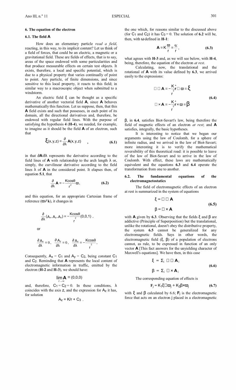
6. The equation of the electron

6.1. The field A

How does an elementary particle read a field, reacting, in this way, to its implicit content? Let us think of a field of forces, that could be an electric, a magnetic or a gravitational field. These are fields of effects, that is to say, areas of the space endowed with some particularities and that produce measurable effects on certain test objects. It exists, therefore, a local and specific potential, which is due to a physical property that varies continually of point to point. Any particle, of finite dimensions, and since sensitive to this local property, it reacts to this field; in similar way to a macroscopic object when submitted to a windstorm.

An electric field ξ can be thought as a specific derivative of another vectorial field A, since A behaves mathematically this function. Let us suppose, then, that this A field exists and such that possesses, in each point of its domain, all the directional derivatives and, therefore, be endowed with regular field lines. With the purpose of satisfying the hypothesis 4 (H-4), we needed, for example, to imagine as it should be the field A of an electron, such that

, (6.1)

in that ∂A/∂λ represents the derivative according to the field lines of A with relationship to the arch length λ or, simply, the curvilinear derivative according to the field lines λ of A in the considered point. It elapses then, of equation 5.1, that

, (6.2)

and this equation, for an appropriate Cartesian frame of reference (ϖ ⁄⁄ k), it changes in

Consequently, Ax = C1 and Ay = C2, being constant C1 and C2. Reminding that A represents the local content of electromagnetic information in traffic, emitted by the electron (H-2 and H-3), we should have:

and, therefore, C1 = C2 = 0. In these conditions, λ coincides with the axis z, and the expression for Az it has, for solution

Az = K/r + C3 ,

the one which, for reasons similar to the discussed above (for C1 and C2) it has C3 = 0. The solution of 6.2 will be, then, with ω defined in H-1:

, (6.3)

what agrees with H-3 and, as we will see below, with H-4, being, therefore, the equation of the electron at rest.

Calculating, now, the translational and the rotational of A with its value defined by 6.3, we arrived easily to the expressions:

(6.4)

β, in 6.4, satisfies Biot-Savart's law, being therefore the field of magnetic effects of an electron at rest; and A satisfies, integrally, the basic hypotheses.

It is interesting to notice that we began our arguments using the law of Coulomb, for a sphere of infinite radius, and we arrived in the law of Biot-Savart; more interesting it is to verify the mathematical reversibility of this theoretical road: it is possible to leave of the law of Biot-Savart and to arrive in the law of Coulomb. With effect, these laws are mathematically equivalent and the equations 6.3 and 6.4 operate the transformation from one to another.

6.2. The fundamental equations of the electromagnetostatics

The field of electromagnetic effects of an electron at rest is summarized in the system of equations

ξ = ∇ ⊗ A (6.5)

β = ∇ × A

with A given by 6.3. Observing that the fields ξ and β are addictive (Principle of Superposition) but the translational, unlike the rotational, doesn't obey the distributive property, the system 6.5 cannot be generalized for any electromagnetic fields. Says in other words, the electromagnetic field (ξ, β) of a population of electrons cannot, as rule, to be expressed in function of an only vector A [This fact answers for the unyielding character of Maxwell's equations]. We have then, in this case

ξ = Σi ∇ ⊗ A i (6.6)

β = Σi ∇ × A i

The corresponding equation of effects is

Fj = K1ξ⊗ϖ j + K2β×ϖj (6.7)

with ξ and β calculated by 6.6; Fj is the electromagnetic force that acts on an electron j placed in a electromagnetic

z)y,(x,z)y,(x, Aλ∂∂=ξ

ϖr

Kcos2

θ−=λ∂∂ A

, r

KcosA, A, A

or

, (0,0,1)r

Kcos)A,A,A(

zyx

zyx

2

2

θ−=λ∂

∂=λ∂

∂=

λ∂∂

θ−=λ∂∂

00

(0,0,0)limr

=∞→A

rrK ωϖ ==A

β

ξ

ϖ

ϖ

=×−=×∇

=⊗−=⊗∇

2

2

^

^

rA

rA

r

K

r

K


stationary field; K1 and K2 are constant. The equations 6.5 and 6.6 keep, in its contents, the totality of the electromagnetostatics (with the exception of an important factor related to the induction field τ, mentioned in the item 3.3). 6.3. The scalar electromagnetic field

It is possible40 to consider the electromagnetic field of an electron through a scalar function ϕ given for

ϕ = K/r . (6.8)

For this, it is enough to define ξ and β through the expressions

(6.9)

and to observe that the function ϕ enjoys the following properties

(6.10)

It is gotten, in this way, and without difficulties, to demonstrate that

ξi = ∇ ⊗ Ai e βi = ∇ × Ai

being demonstrated, like this, the compatibility between 6.8 and 6.3. 6.4. The electromagnetic information (e.m.i.)

The equations 6.9 show us that the electromagnetic field (ξ,β) of the electron can be described in terms of gradient of a function of position ϕ. We can, then, to conjecture about the actual existence of something emitted by the electron and to call, at this something, by electromagnetic information (e.m.i.). The equation 6.8 suggests still more: the e.m.i., once emitted, they are conserved. In other words, the electron is an emitter source of e.m.i.; and the e.m.i. flow that crosses a surface any, identifies with the flow of a vectorial field h expressed by

h = - ∇ ϕ (6.11)

It is implicit in these considerations that h is of the type h = ρc , being ρ an invariant that represents the local density of e.m.i., and c is the speed with that these e.m.i. spreads in an appropriate reference system. 7. Field-reference frame relationship

7.1. The inertial systems

A Coulomb�s electric load, when passing of at rest state to another one, in a rectilinear and uniform movement, emits, during this phase of acceleration, an aura that defines two universes: a) an interior universe, that already contains the field of the load adapted to its inertial movement; in this universe, everything happens as if the

40 MESQUITA F.°, A. (1996): Sobre a natureza físico-matemática do

elétron, Integração II(4):26-30.

load was at rest in a reference frame that travels with the load, in uniform movement; b) and other external universe, that contains the field of the load in rest in the initial inertial reference frame.

The aura consists of a mobile membrane, of finite thickness, and that is headquarters of a mutant field, to which we got used to call for electromagnetic radiation. This aura, when crossing an area of the space, to a very certain speed, promotes the transformation of the inertial field (that of the load at rest) in other (that of the load at rectilinear and uniform movement).

This phenomenon also happens with electrons, since accelerated in specific directions as, for example, in an electric current, or enter the plates of a capacitor or, still, when dropping in direction to the nucleus of an atom, when changing of orbit.

How would the field of an electron be in a non inertial system of reference? How would the equation of the electron be in those circumstances?

We saw the equation 6.3 of the electron at rest in the reference system in that we lived. The founded function doesn't exhibit any dependence with relationship at the time. We can suspect, however, that the equation of the electron at rest, in an accelerated reference system, it should show some dependence with relationship at the time. And we could also admit that, in an allowed orbit, the equation of the electron (obtained in a reference frame that accompanied it in this movement) should behave a solution different from 6.3 and such that was periodic and looking a stationary character.

The presented equations, in the previous items, were deduced in a very special reference system, that is to say, in the reference frame of the laboratory of Coulomb, or still, in the frame of reference in which Newton deduced the laws of the mechanics. What should be made to generalize them? What is an inertial reference system?

The success of the classic mechanics is more than enough to guarantee us the existence of the inertial systems. In spite of this, the classic mechanics didn't get to define an inertial frame of reference. Using the words of Einstein and Infeld, the classic mechanics floats in the air, because we didn't meet any rule to determine an inertial system.41

At the end of the century XIX, the physicists tried to define the inertial systems, in a such way that could stay adjusted to the classic mechanics. The adopted logic was the one of trying to consider them through field theories, of the which the including was Maxwell's theory. In this way, they tried to characterize a Maxwellian inertial frame of reference. This reference frame, however, it was shown incompatible with the Newtonian inertial reference systems.42 Of this incompatibility, the relativistic physics of Einstein appeared.

We are, in this work, trying to interpret the electromagnetism in a different way of the habitually adopted; it is arrived the moment, therefore, of we try to abolish this incompatibility. I will say, then, that

41 EINSTEIN,A.; L.INFELD: A evolução da física, Zahar Ed., Rio de

Janeiro, 1980. 42 BUNGE,M., Controvérsias em física, Editorial Tecnos S.A.,

ϖβϖξ iiiiii e ×ϕ∇=⊗ϕ∇=

)(

)(

ϖϖ

ϖϖ

ϕ×∇=×ϕ∇

ϕ⊗∇=⊗ϕ∇


C-7: Corollary 7

An inertial system of reference is that in which the equation of the electron at rest is A = ω/r, being observed the fields of effects, defined by the equations 6.5.

7.2 Appropriate and not appropriate reference frames

I will say that an appropriate frame of reference is that in which the electron in study maintains P and ω constants. It is, therefore, the frame of reference adapted for the mathematical analysis of the electromagnetic field of the electron, because this field is function of ω and r. In particular, if the appropriate frame of reference is inertial, the electromagnetic field of the electron will just be function of these two variables (equations 6.5). In the remaining of this work we will just study fields produced by electrons placed in appropriate and inertial frame of reference.

7.2.1. Observer placed in a non appropriate reference frame

The fields ξ and β, when observed through a non appropriate reference frame, they manifest an effect that links to a phenomenon described by Liénard (1898) and Wiechert (1900) for the potentials of Maxwell's theory. This phenomenon should be analyzed with extreme caution, because ξ and β are functions of two variables (ϕ and ω). Both contributions are interesting, but that owed ω acquires epistemological importance because, not being taken in consideration, it generates fateful consequences for the classic physics.43 The non consideration of this portion placed in evidence the fundamental stone on which leaned on the theory of the relativity of Einstein.

Let us see, in first place, as ϕ it is transformed. With the considerations made in the item 6.4, expressed by the equation 6.11, we can admit that, being ρ an invariant, h (and consequently ϕ) it is transformed according to:

h = ρc ⇔ h' = ρc' ,

in which c' = c + v, being v the speed of the e.m.i. emitter electron, when observed of the non appropriate frame of reference.

Let us see, now, like ω it is transformed. Let us consider, then, an observer placed in a Q point of an inertial frame of reference, and an electron, placed in a point P and moving, in relation to this inertial system, with a constant speed v. I will say then that the ϖ unitary vector appears, for the observer in Q, as if it was another unitary vector, ϖ�, that is to say, it suffers an aberration, conserving its unitary module.44 For the calculation of this aberration, observed the conventions adopted in the figure 11, the following should be made:

43 This subject is discussed with more details in the article MESQUITA

F.°, A. (1996): Sobre a natureza físico-matemática do elétron, Integração II(4):26-30.

44 MESQUITA F.°, A. (1996): Sobre a natureza físico-matemática do elétron, Integração II(4):26-30.

1) to determine the point P', being admitted that the field spreads in a radial way and with a speed c, when analyzed of the appropriate frame of reference;

2) to attach the points P, P' and Q; 3) to trace a cone with the vertex in P, and that

contains ϖ in its surface, and with the axis in the direction PQ;

4) to transfer the cone, together with ϖ, for P'; 5) to rotate the cone around P' and in according to a

perpendicular axis to the plan of the figure (plane PP'Q), until that the axis of the cone locates in the direction P'Q.

6) the unitary vector obtained by this rotation of ϖ it is ϖ�.

ω̂γ

ω̂

γr'r

v v

Q

P' P

ω̂'

Figure 11: Aberration of ϖ (ϖ ⇒ ϖ�) . P = position of the electron in an instant t in relation to an inertial frame of reference not appropriate and where the electron travels to a speed constant v, maintaining constant ϖ and in which the observer is in rest in Q. P' = position of the electron in an instant delayed t', in which the field that arrives in Q, in the instant t, was generated.

As I marked in previous article, the scalar K of the hypothesis 1 (and, therefore, the absolute value of the vector ω), it seems to contain secrets related to the inertial frame of reference that only the experimental physics can decipher. It would be extremely interesting to verify if its absolute value, once defined, it stays or not identical, any that is the considered inertial frame of reference. The variability of K, as I believe, would be an indication strongly suggestive to corroborate Newton's intuition with relationship to the existence of an absolute reference system. It can be waited, however, that K stays constant for v << c.

7.3. The (ξ, β) field of the electron in movement

Known the transformations for h and ϖ, we can despise the apostrophes and to assume that the fields ξ and β of an electron are expressed for

ξ = -h ⊗ ϖ β = -h×ϖ (7.1)

so much in the appropriate reference system as in the non appropriate reference system. It elapses, then, of 7.1, that, any that is the considered inertial frame of reference, the sum ξ2 + β2 is a classic relativistic function of position:

h2 = ξ2 + β2


8. Final considerations Among the consequences that can result of the

acceptance of this new electromagnetic theory, some were already commented. Countless another will appear with its development. It would be interesting, however, that before we contain the narrative, we comment some thing regarding the fields of effects ξ and β.

In first place it is important to stress that ξ and β are isodimensional and, although looked physically with the fields of Maxwell's theory, they represent different variables. In particular, and as already commented, ξ and β are fields that act on electrons (protons), while the classic fields act on populations of electrons (protons) that assemble, in the space, under a very capricious and a very special structure. It elapses of these differences that in certain local where the classic fields are null, the electrons behave as if were submitted to a field of forces, classified as inexplicable; for example, the electromagnetic field of a solenoid that, in its exterior, it induces a change in the pattern of interference of electrons.45 Something similar it happens inside a electrically loaded conductor and, therefore, where E = 0. The theory, for now presented, it foresees that, in these conditions, an electron, known the conditions of its entrance in this field, it will describe a trajectory not classic and not inertial, and, nevertheless, theoretically previsible, without the aid of the quantum logic.

We will go now, to comment some thing regarding interesting aspects related to the field of magnetic effects β. In first place, it can seem strange, to the reader, that an electron at rest generates a field of magnetic effects. This verification leans on in the developed logic; and there is not report of experiences that contradict this theoretical expectation. What exists, truly, it is the observation that the effect of a magnetic field B, on an electron, depends on the speed of this electron in relation to a convenient reference system. This dependence, appears in two opportunities: the first, in the characterization of the magnetic field B; and the other, in the equation of force of Lorentz. In both cases, the dependence is lineal, and the considered speed it is the same. Let us see, now, as to solve this supposed contradiction.

An electron, when entering in an electromagnetic field of the type (ξ=0, β), with constant β, and with an initial speed v, perpendicular to the lines of the field β, acquires a helicoidal and uniform movement with radius R. Consequently, we have:

being m the inertial mass of the electron. Equaling the expression for F, obtained above, with

that obtained in the item 6.2 (equation 6.7), we have:

45 FEYNMAN,R.; R.B.LEIGHTON: Física, vol. 2, Electromagnetismo y

matéria, Addison-Wesley Iber., 1987, p.15-11.

Two conclusions elapse of this equality: 1) the first links to the orientation of the electron in a field β; if we thought in the vector ϖ as a spin, we can say that this spin is conducted, in this field, according to the trajectory of the electron; the accountable by this orientation it is the induction field τ. 2) The constant K2 is actually a variable dependent of the speed of the electron:

K2 = f(vn2) = Kmεvn2

vn is the component of v in the perpendicular direction to β (for the case described vn = v); Km is the constant that correlates cause to magnetic effect; and ε it is a convenient constant, equal at -1 for electrons and equal at 1 for protons. In consequence, the equation of effects (6.7) can be expressed for

F = Keεξ ⊗ ϖ + Kmεv n2β×ϖ

being Ke the constant that correlates cause to electric effect. This equation corresponds to the equation of Lorentz, valid for an electron (proton).

Finally, we will comment some thing regarding the physical-mathematical nature of the fields of effects. We already said that the fields ξ and β are not Gaussian. If we render attention to the electric action and reaction among two electrons, represented in the figure 10, we will notice, also, that the field ξ it is not Newtonian, fact this that also happens with the field β. In terms of force, and being thought exclusively in two electrons, there is not as to speak in equality between action and reaction. It is important to mark, nevertheless, that this, by itself, is not going against the Newtonian mechanics. In dynamic conditions, as it is the case of the figure 10, action and reaction not always they are translated exclusively by forces: an electron also modifies the field of the other, and this modification spreads under the form of non stationary e.m.i. or, using the classic language, under the form of radiant energy. To this action it also corresponds a reaction, which should also be asymmetric. The asymmetries (forces and emission of energy) should be of such equivalent order that they are compensated, through the lineal and angular conservation of moments.

As final message, I transcribe the thought exposed in the foreword of the original edition: When writing this theory I tried to collaborate so that we could come back to the time in that the physics was an intelligible science. In search of this ideal, Schrödingler, DeBroglie, Dirac, Einstein and so many other gave us its lives. Let us know how then to use the trail bequeathed to us by the wise masters.

* * * * *

This article is protected by the copyright laws, being therefore forbidden the reproductions as well as the commercialization without the authorization expressed by the author. Comments and suggestions can be guided to the author through the e-mail [email protected]

^RF

Rmv2

-=

^R

RmvK

2

2 -=× ϖβ

Documents

The equation of the electron and the · PDF fileThe equation of the electron and the electromagnetism A new unifying electromagnetic theory Alberto Mesquita Filho * ... 2 FEYNMAN,R.;