Embed Size (px)
Citation preview

THE ENVIRONMENTAL IMPACT AND SUSTAINABILITY
APPLIED GENERAL EQUILIBRIUM (ENVISAGE) MODEL
Version 7.1
Dominique van der Mensbrugghe
The World Bank
December, 2010
Abstract: This document's main purpose is to provide a full description of the World Bank's
global dynamic computable general equilibrium model known as ENVISAGE. ENVISAGE has
been developed to assess the interactions between economies and the global environment as
affected by human-based emissions of greenhouse gases. At its core, ENVISAGE is a relatively
standard recursive dynamic multi-sector multi-region CGE model. It has been complemented by
an emissions and climate module that links directly economic activities to changes in global
mean temperature. And it incorporates a feedback loop that links changes in temperature to
impacts on economic variables such as agricultural yields or damages created by sea level rise.
One of the overall objectives of the development of ENVISAGE has been to provide a greater
focus on the economics of climate change for a more detailed set of developing countries as well
as greater attention to the potential economic damages. The model remains a work in progress as
there are several key features of the economics of climate change that are planned to be
incorporated in coming months.

- ii -
Table of contents
INTRODUCTION ....................................................................................................................................................... 1
MODEL SPECIFICATION ....................................................................................................................................... 2
PRODUCTION BLOCK .................................................................................................................................................. 2 INCOME BLOCK .......................................................................................................................................................... 6 DEMAND BLOCK ........................................................................................................................................................ 8
Expenditures ........................................................................................................................................................ 9 THE FUELS BLOCK ................................................................................................................................................... 11 TRADE BLOCK .......................................................................................................................................................... 15
Top level Armington ........................................................................................................................................... 15 Second level Armington nest .............................................................................................................................. 17 Export supply ..................................................................................................................................................... 17 Homogeneous traded goods ............................................................................................................................... 19 Domestic supply ................................................................................................................................................. 20 International trade and transport services ......................................................................................................... 21
PRODUCT MARKET EQUILIBRIUM ............................................................................................................................. 22 FACTOR MARKET EQUILIBRIUM ............................................................................................................................... 22
Economy-wide factor markets ............................................................................................................................ 22 Labor markets .................................................................................................................................................... 23 Sector-specific factor markets ............................................................................................................................ 24 Capital markets with the vintage capital specification ...................................................................................... 25 Allocation of Output across Vintages................................................................................................................. 27
MACRO CLOSURE ..................................................................................................................................................... 28 MODEL DYNAMICS .................................................................................................................................................. 30 EMISSIONS , CLIMATE AND IMPACT MODULES .......................................................................................................... 31
Greenhouse gas emissions ................................................................................................................................. 32 Emission taxes, caps and trade .......................................................................................................................... 32 Concentration, forcing and temperature ............................................................................................................ 33 Climate change economic impacts ..................................................................................................................... 35
REFERENCES .......................................................................................................................................................... 38
ANNEX 1: THE CES/CET FUNCTION ................................................................................................................. 40
THE CES FUNCTION ................................................................................................................................................ 40 CALIBRATION .......................................................................................................................................................... 42 THE CET FUNCTION ................................................................................................................................................ 42
ANNEX 2: THE DEMAND SYSTEMS ................................................................................................................... 44
THE CDE DEMAND SYSTEM ..................................................................................................................................... 44 THE ELES DEMAND SYSTEM ................................................................................................................................... 51 THE AIDADS DEMAND SYSTEM .............................................................................................................................. 54
ANNEX 3: ALTERNATIVE TRADE SPECIFICATION ..................................................................................... 61
ANNEX 4: ALTERNATIVE CAPITAL ACCOUNT CLOSURES ...................................................................... 62
ANNEX 5—DYNAMIC MODEL EQUATIONS WITH MULTI-STEP TIME PERIODS ............................... 63
DYNAMICS IN A MULTI-YEAR STEP .......................................................................................................................... 63
ANNEX 6: CLIMATE MODULES.......................................................................................................................... 65
DICE 2007 CLIMATE MODULE ................................................................................................................................ 65 Emissions and concentration ............................................................................................................................. 66 Temperature ....................................................................................................................................................... 70

- iii -
ANNEX 7: EXAMPLES OF CARBON TAXES, EMISSION CAPS AND TRADABLE PERMITS ................ 73
BORDER TARIFF ADJUSTMENT SIMULATIONS ........................................................................................................... 73
ANNEX 8: BASE ENVISAGE PARAMETERS ..................................................................................................... 77
ANNEX 9: THE ACCOUNTING FRAMEWORK ................................................................................................ 81
ANNEX 10: DIMENSIONS OF GTAP RELEASE 7.1 .......................................................................................... 86
FIGURES ................................................................................................................................................................... 90

- 1 -
Introduction
The purpose of this document is to provide a complete specification of the equations of the
World Bank’s ENVIRONMENTAL IMPACT AND SUSTAINABILITY APPLIED GENERAL EQUILIBRIUM
(ENVISAGE) MODEL. The ENVISAGE Model is designed to analyze a variety of issues related
to the economics of climate change:
Baseline emissions of CO2 and other greenhouse gases
Impacts of climate change on the economy
Adaptation by economic agents to climate change
Greenhouse gas mitigation policies—taxes, caps and trade
The role of land use in future emissions and mitigation
The distributional consequences of climate change impacts, adaptation and
mitigation—at both the national and household level.
ENVISAGE is intended to be flexible in terms of its dimensions. The core database—that
includes energy volumes and CO2 emissions—is the GTAP database, currently version 7.1 with
a 2004 base year. The latter divides the world into 112 countries and regions, of which 95 are
countries and the other region-based aggregations.1 The database divides global production into
57 sectors—with extensive details for agriculture and food and energy (coal mining, crude oil
production, natural gas production, refined oil, electricity, and distributed natural gas). Annex 8
provides more detail. Due to numerical and algorithmic constraints, a typical model is limited to
some 20-30 sectors and 20-30 regions.
This document describes the current version of ENVISAGE, which is still in a developmental
stage. This current version includes the following:
Capital vintage production technology that permits analysis of the flexibility of
economies
A detailed specification of energy demand in each economy, with additions yet to come
(see below)
The ability to introduce future alternative energy (or backstop) technologies
CO2 emissions that are fuel and demand specific
Incorporation of the main Kyoto greenhouse gases (methane, nitrous oxide and the
fluoridated gases)
A flexible system for incorporating any combination of carbon taxes, emission caps and
tradable permits
A simplified climate module that links greenhouse gas emissions to atmospheric
concentrations combined with a carbon cycle that leads to radiative forcing and
temperature changes.
The future work program includes the following tasks:
1 The countries defined in GTAP cover well over 90 percent of global GDP and population. The country
coverage is weakest for Sub-Saharan Africa and the Middle East—though with ongoing work to extend the
country coverage.
- 2 -
Adding a resource depletion module for coal, oil and gas
Addition of marginal abatement cost curves for the non-CO2 gases
Adding a more detailed land-use module
Adding additional alternative technologies
Model specification
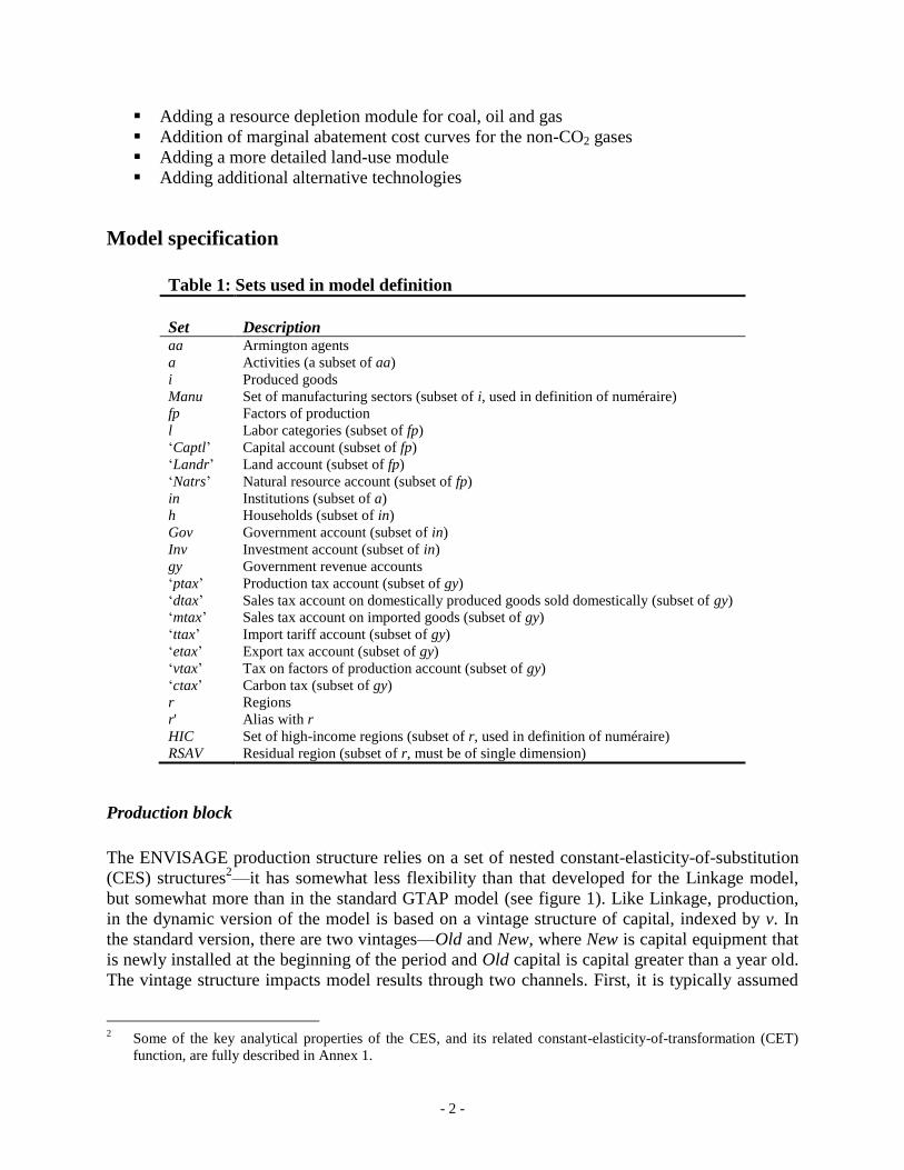
Table 1: Sets used in model definition
Set Description aa Armington agents
a Activities (a subset of aa)
i Produced goods
Manu Set of manufacturing sectors (subset of i, used in definition of numéraire)
fp Factors of production
l Labor categories (subset of fp)
‘Captl’ Capital account (subset of fp)
‘Landr’ Land account (subset of fp)
‘Natrs’ Natural resource account (subset of fp)
in Institutions (subset of a)
h Households (subset of in)
Gov Government account (subset of in)
Inv Investment account (subset of in)
gy Government revenue accounts
‘ptax’ Production tax account (subset of gy)
‘dtax’ Sales tax account on domestically produced goods sold domestically (subset of gy)
‘mtax’ Sales tax account on imported goods (subset of gy)
‘ttax’ Import tariff account (subset of gy)
‘etax’ Export tax account (subset of gy)
‘vtax’ Tax on factors of production account (subset of gy)
‘ctax’ Carbon tax (subset of gy)
r Regions
r' Alias with r
HIC Set of high-income regions (subset of r, used in definition of numéraire)
RSAV Residual region (subset of r, must be of single dimension)
Production block
The ENVISAGE production structure relies on a set of nested constant-elasticity-of-substitution
(CES) structures2—it has somewhat less flexibility than that developed for the Linkage model,
but somewhat more than in the standard GTAP model (see figure 1). Like Linkage, production,
in the dynamic version of the model is based on a vintage structure of capital, indexed by v. In
the standard version, there are two vintages—Old and New, where New is capital equipment that
is newly installed at the beginning of the period and Old capital is capital greater than a year old.
The vintage structure impacts model results through two channels. First, it is typically assumed
2 Some of the key analytical properties of the CES, and its related constant-elasticity-of-transformation (CET)
function, are fully described in Annex 1.

- 3 -
that Old capital has lower substitution elasticities than New capital. Thus countries with higher
savings rates will have a higher share of New capital and thus greater overall flexibility. The
second channel is through the allocation of capital across sectors. New capital is assumed to be
perfectly mobile across sectors. Old capital is sluggish and released using an upward sloping
supply curve. In sectors where demand is declining, the return to capital will be less than the
economy-wide average. This is explained in greater detail in the market equilibrium section.
Most of the equations in the production structure are indexed by v, i.e. the capital vintage. The
exceptions are those where it is assumed that the further decomposition of a bundle are no longer
vintage specific—such as the demand for non-energy intermediate inputs. Each production
activity is indexed by a, and is different from the index of produced commodities, i (allowing for
the combination of outputs from different activities into a single produced good, for example
electricity).
(P-1) var
var
varv
var
cd
ar
va
varvar XPvPVA
PXvVA
pvar
pvar
,,
,,
,,1
,,,,,,,
,,
,,
(P-2)
v
var
ar
varn
var
cd
ar
nd
varar XPvPND
PXvND
pvar
pvar
,,
,
,,1
,,,,,,
,,
,,
(P-3)
)1/(11
,,
,
,,
1
,,
,,
,,
,
,,
,,,,,
1
pvarp
jrp
var
n
var
arnd
varv
var
varva
varcd
ar
var
PNDPVAPXv
(P-4) ar
v
varvar
ararXP
XPvPXv
PX,
,,,,
,, )1(
(P-5) v
varvararar XPvPXv ,,,,,,
(P-6) x
arar
p
arar PXPP ,,,, )1(
Equations (P-1) and (P-2) are derived demands for two bundles, one designated as aggregate
value added, VA, though it also includes energy demand that is linked to capital, and aggregate
intermediate demand, ND, a bundle that excludes energy. Both are shares of output by vintage,
XPv, with the shares being price sensitive with respect to the ratio of the vintage-specific unit
cost, PXv, and the component prices, respectively PVA and PND. The equations allow for
technological change embodied in the parameters that are allowed to be node-specific. For
uniform technological change, the two parameters can be subject to the same percentage change.
Both productivity factors are impacted by the same damage adjustment, cd
, which is region and
sector specific and depends on climate change.3 Equation (P-3) defines the vintage-specific unit
3 Discussed further below.

- 4 -
cost, PXv. Almost all CES price equations are based on the dual cost function instead of the
aggregate cost or revenue formulation. The unit cost function includes the effects of productivity
improvement and damages. To the extent climate leads to damages, cd
drops below its initial
level of 1, raising unit cost, all else equal. Equation (P-4) determines the aggregate unit cost, PX,
the weighted average of the vintage-specific unit costs with the weights given by the vintage-
specific output levels. The model allows for a markup, , to unit cost that is normally exogenous
and initialized at 0. The revenue generated by the markup, , is defined in equation (P-5).
Equation (P-6) determines the final market price for output, PP, that is equal to the unit cost
augmented by the output tax (or subsidy), p. The equivalence of the tax-adjusted unit cost to the
output price is an implication of assuming constant-returns-to-scale technology and perfect
competition (and/or the presence of a fixed markup). The production price can also be adjusted
by a volume only tax (or an excise tax), represented by x.
The subsequent production nest decomposes the VA bundle (value added and energy) into non-
capital factors of production on the one hand, XF, indexed by fpx4, and the capital/energy bundle
on the other hand, KE. The key substitution elasticity is given by v. An elasticity of 1 implies a
Cobb-Douglas technology.5
Equation (P-7) determines the demand for non-capital factors
(unskilled and skilled labor, land, and a sector-specific factor if it exists).6 Factor productivity is
given by the factor. The productivity factor is 'climate sensitive', in other words, it is a
combination of a baseline growth assumption that is also sensitive to changes in global climate
as measured by the change in global mean temperature. This is explained further below.
Equation (P-8) determines demand for the capital/energy bundle, KE. The final equation in this
nest (P-9) defines the unit price of the value added cum energy bundle, PVA.
(P-7) , ,
, , 1, ,
, , , , , , , , ,
, ,
vr a v
vr a v r a vd f gf
r fpx a r fpx a v r fpx a r a v
v r fpx a
PVAXF VA
PF
(P-8) var
var
varke
varvar VAPKE
PVAKE
vvar
,,
,,
,,
,,,,
,,
(P-9)
, ,, ,
, ,
1/(1 )1
1, ,
, , , , , , , , ,
, ,
vr a vv
r a v
vr a vr fpx af ke
r a v r fpx a v r a v r a vgffpx r fpz a
PFPVA PKE
The next nest is a decomposition of the capital/energy bundle, KE, into demand for capital (by
vintage) and an energy bundle. Equation (P-10) defines the demand for capital by vintage, KV.
The substitution elasticity is given by ke
. Equation (P-11) determines the demand for the energy
4 The set fp indexes all factors of production, the subset fpx excludes capital.
5 In the GAMS implementation of the model, a Cobb-Douglas technology is approximated by an elasticity of
1.01. 6 The model implementation allows for a scale factor (phiw) that is used to scale factor prices. This can help with
numerical problems.

- 5 -
bundle, XNRG. The latter is indexed by eb, a special set that indexes all energy bundles. There is
a set mapping that has a one-to-one correspondence between the given activity a and a specific
item in eb. The reason for this is to simplify the code for disaggregating the energy bundles
across agents in the economy and is described further below. Equation (P-12) defines the price of
the KE bundle, PKE.
(P-10) , ,
, , 1, ,
, , , , , , , , , ,
, ,
ker a v
ker a v r a vf gf
r a v r Captl a v r Captl a v r a v
r a v
PKEKV KE
PKV
(P-11) var
vebr
varep
varvebr KEPNRG
PKEXNRG
kevar
,,
,,
,,
,,,,
,,
(P-12)
, ,, ,
, ,
1/(1 )1
1, ,
, , , , , , , , ,
, ,
ker a vke
r a v
ker a vr a vf ep
r a v r Captl a v r a v r eb vgf
r Captl a
PKVPKE PNRG
The final node in the production nest is the decomposition of aggregate demand for non-fuel
intermediate goods, ND. For the moment, we are assuming a standard Leontief technology
(although allowing for the possibility of substitution across inputs.7 Equation (P-13) determines
the demand for the (Armington) intermediate demand for non-fuel inputs, XAn, with the
substitution elasticity given by n. The relevant price is the agent (or activity) specific
Armington price, PAa. The latter will be a composite price of domestic and imported goods,
augmented by domestic taxes and, in mitigation scenarios, with a tax linked to emissions
(described below). The model allows for input-specific efficiency improvements as encapsulated
by the nd
parameter. Equation (P-14) provides the price of the aggregate ND bundle.
(P-13) ara
anr
arnd
anrOldanranr NDPA
PNDioXA
nar
nar
,
,,
,1
,,,,,,,
,
,
(P-14)
)1/(11
,,
,,
,,,,
,,
narn
ar
nnrgnnd
anr
a
anr
Oldanrar
PAioPND
This ends the description of the production structure, though there is a further decomposition of
XAn, i.e. the non-fuels intermediate Armington demand, and the energy bundle. The latter is
decomposed across fuels, and then finally decomposed as an Armington good.
7 The Linkage model has a different production structure for crops, livestock and all other goods allowing for
more complex interactions between agricultural inputs, for example fertilizers and feed, and the factors of
production.

- 6 -
Income block
The model has six indirect tax streams and one direct-tax stream:
1. The output tax, p imposed on the aggregate price of output, PX, with an additional excise
tax, x, in some circumstances.
2. A sales tax on sales of domestic Armington goods, Ap
, which is agent specific and
imposed on the economy-wide price of domestic goods, PA.8
3. Bilateral import tariff, m, imposed on the landed (or CIF) price of imports, WPM. The
model also allows for homogeneous goods, in which case the tariff represents a wedge
between the world price and the domestic price.
4. Bilateral export tax (or subsidy), e, imposed on the producer price of exports, PE. In the
case of a homogeneous commodity, the export tax represents the wedge between world
prices and domestic prices.
5. Taxes on the factors of production, v, imposed on the market-clearing price of factors,
NPF.
6. Taxes on emissions, e, imposed on the Armington consumption of goods.
Equations (Y-1) through (Y-6) correspond to the aggregate revenues generated by each of the six
indirect taxes. The notation for the variables not already described will be given below. One
important observation concerns the bilateral trade variables. These are always indexed as (r, r', i)
where r is the country of origin (the exporter), r' the country of destination (the importer) and i is
the sector index. This explains the switch in the indices equations (Y-3) and (Y-4) where WTF
corresponds to the bilateral trade flow from region r to region r'. Carbon tax revenues will be a
function of the parameter that allows for full or partial participation—including full
exclusion—by agent. Equation (Y-7) defines the aggregate revenue from taxing household
income. Fiscal closure will be discussed below.
8 The model allows for agent-specific Armington decompositions, though this increases the size of the model
considerably. This is described further in Annex 3 on alternative trade specification.

- 7 -
(Y-1) a
ar
x
ararar
p
arptaxr XPXPPXGREV ,,,,,,
(Y-2) i aa
aairir
c
aair
Ap
aairataxr XAPATGREV ,,,,,,,, )(
(Y-3)
Armi
iri
m
ir
Armi r
d
irrirr
m
irrttaxr XMTPWWTFWPMGREV ,,
'
,,',,',,',
(Y-4)
Armi
iri
e
ir
Armi r
s
irrirr
e
irretaxr XETPWWTFPEGREV ,,
'
,',,',,',,
(Y-5) fp a
afprafpr
v
afprvtaxr XFNPFGREV ,,,,,,,
(Y-6) , , , , , , , , , ,
emi e
r ctax r em r em i aa em r em i aa r i aa
em i aa
GREV XA
(Y-7) r
h
hr
k
rhtaxr YHGREV ,,
Equation (Y-8) defines aggregate fiscal revenues, where the set gy corresponds to the six indirect
tax streams (ptax, atax, ttax, etax, vtax and ctax) and the direct tax stream (htax). It is also
assumed that income from a cap and trade system on emissions accrue to the government.
Equation (Y-9) summarizes net household income, YH. It is assumed that all factor income net of
factor taxes (where NPF represents the market clearing factor price net of taxes) accrues to
households as well as profits generated by the markups. Household income is then adjusted for
the depreciation allowance, DeprY. Equation (Y-10) describes household disposable income, YD,
where h represents the base year household-specific direct tax rate. The direct tax rate is
adjusted by an economy-wide adjustment factor, k, which can be endogenous to achieve a given
target, for example the deficit of the public sector. Macro closure is discussed in more detail
below.9 Disposable income is adjusted by changes in international tourism receipts, IIT, which
will be affected by climate change.
9 The GTAP dataset contains only a single representative household per country/region. The model
implementation allows for multiple households and hence the need for an economy-wide tax shifter that is
uniform across households. This has different distributional consequences than an additive shifter or a more
complex direct tax schedule.

- 8 -
(Y-8) em
E
em
gy
gyrr QuotaYGREVYG ,
(Y-9) r
a
ar
fp a
afprafprr DeprYXFNPFYH ,,,,,
(Y-10) , ,1 k h
r r r h r r hYD YH IIT
Demand block
The demand block is divided into two sections. The first describes the allocation of household
disposable income between savings and expenditures on goods and services. The second
describes other final demand for goods and services.
Households first allocate total expenditures between savings on the one hand and aggregate
expenditures on goods and services on the other hand.10
Equation (D-1) determines the
household savings rate (relative to disposable income), ss, as a function of per capita growth (g
pc)
and the youth and elderly dependency ratios, respectively given by DRATPLT15
and DRATP65UP
.11
These variables are typically exogenous in dynamic scenarios. The savings function also
captures a persistence factor defined by s.12
Equation (D-2) determines the level of household
savings. It should be noted that if the ELES utility function is used to specify household demand
for goods and services, equation (D-1) is dropped and equation (D-2) then defines the average
propensity to save as the ELES itself determines the level of savings. Equation (D-3) in essence
determines aggregate expenditures on household goods and services, YC. In the case of the
ELES, combined with equation (D-4), it defines the level of household savings, which is an
outcome of the ELES. Equation (D-4) is only used for the ELES version of the model.
10
The demand block is significantly reformulated compared to the first version of the ENVISAGE model. The
latter was largely inspired by the GTAP model. The current version is more similar to the Linkage specification.
It drops the top level utility function that allocated national income across savings, and public and private
expenditures. In the long-term scenarios this top-level structure was typically over-ruled with other specific
assumptions making the theoretical consistency of the top-level formulation less appealing. 11
The original theory and parameters for this formulation can be found in Loayza et al 2000 and Masson et al
1998 and is summarized in van der Mensbrugghe 2006. 12
Setting all the parameters to 0 would yield a constant savings rate. It is also possible to use this equation to
formulate a different closure—for example to target investment and allow the shift parameter, s, to adjust to
achieve the given target.

- 9 -
(D-1) UPP
r
e
r
PLT
r
y
r
pc
r
g
r
s
hr
s
r
s
hr
s
r
s
hr DRATDRATgss 6515
1,,,,
(D-2) hr
s
hr
h
hr YDsS ,,,
(D-3) h
hrhrhr SYCYD ,,,
(D-4) k
hkrhkrhr XHPHXYC ,,,,,
Expenditures
The next block of equations determines the sectoral demands for goods and services for
households. In the standard model private expenditures are derived from the AIDADS
specification and are based on consumer-defined goods, XH, indexed by k, not Armington goods,
XA, that are indexed by i.13
Equations (D-5) and (D-6) are used for three demand systems—LES,
ELES and AIDADS. Equation (D-5) defines supernumerary income, Y*, residual income after
subtracting expenditures on subsistence minima. (In the case of the ELES, savings is added to
YC as the savings decision is part of the allocation of disposable income and not determined
independently. Thus e equals 1 for the ELES implementation and 0 for all others.) Equation
(D-6) determines household expenditure on good k. It is composed of two factors. The first
factor represents expenditures on the subsistence minimum, gh
, or floor expenditures. These are
calibrated on a per capita basis and are therefore multiplied by population to get the total volume.
The second component is a share of supernumerary income, where is the marginal share and
PHX represents the price of consumer commodity k. In the LES and ELES formulations, the
marginal share parameters are calibrated and fixed. In the AIDADS formula, the marginal shares
are a function of utility (intuitively of income), and thus the marginal shares evolve over time.
Equation (D-7) determines the marginal shares, based on calibrated parameters and . Clearly,
if the two are identical, we are back to an LES/ELES specification. Equation (D-8) defines the
utility level, U—either explicitly or as an implicit function. The CDE implementation is
described fully in Annex 2.
It should be noted that the subsistence minima, though calibrated using base year data, are in
some cases 'climate sensitive'—for example energy demand for cooling and/or heating. This is
described further below. The gh
parameters represent the climate sensitive parameters, whereas
the h are the initial calibrated parameters.
13
Other demand specifications have been implemented and are described in Annex 2. These include both the
linear and extended linear expenditure system (LES and ELES) as well as the CDE specification that is the
standard utility function for the GTAP model. Three of the expenditure systems (CDE, LES and AIDADS) use
a two-tiered nest to allocate savings on the one hand and expenditures on goods and services on the other. The
ELES integrates both in a single-tiered system.

- 10 -
(D-5) *
, , , , , , , ,
e h gh
r h r h r h r h r k h r k h
k
Y YC S Pop PHX
(D-6) , , *
, , , , , ,
, ,
c
r k hgh
r k h r h r k h r h
r k h
HX Pop YPHX
(D-7) ,
,
, , , ,
, ,1
r h
r h
Uad ad
r k h r k hc
r k h U
e
e
(D-8) ,
, ,
, ,
, , ,
, , , , , , , ,
, ,
ln ln( ) 1 ln 1r h
r k h gh
r k h
r k h r hc gh c
r h r k h r k h r h r k h Uk kr h r h
HX
HX PopU A
Pop A e
Equation (D-9) represents the private expenditure budget shares, sh. Equation (D-10) defines a
consumer price index for private consumption, PC. Finally, equation (D-11) defines the volume
of aggregate private consumption, XC.
(D-9) hr
hkrhkrh
hkrYC
HXPHXs
,
,,,,
,,
(D-10) k
hkr
h
hkrhr PHXsPC ,,,,,
(D-11) hrhrhr PCYCXC ,,, /
The next set of equations decomposes consumer demand defined as consumer goods into
produced (or more accurately, Armington) goods. A transition matrix approach is used where
each consumed good is composed of one or more produced goods and combined using a CES
aggregator.14
Each consumer good could also have its own energy bundle—with different
demand shares across energy.15
Equation (D-12) converts consumed goods HX into non-energy
Armington goods, XA. Equation (D-13) determines demand for the energy bundle, XNRG, for
each of the k consumed goods. There is a one-to-one correspondence between each index k and
an index in the set eb (that also includes demand for energy bundles in production and other final
demand). Equation (D-14) then determines the price of consumer good k.
14
Using the standard GTAP data, the transition matrix is diagonal—each consumed good corresponds to exactly
one produced good. ENVISAGE still uses this approach save for the energy bundle that is combined into one
consumed commodity. Work is ongoing to develop a global database of transition matrices. The GREEN model
for example (see Burniaux et al 1992 and van der Mensbrugghe 1994) had four consumed goods and eight
standard produced goods. 15
For example, a transportation bundle is likely to be dominated by liquid fuel demand, whereas demand for heat
is likely to be dominated by electricity and natural gas.

- 11 -
(D-12) hkr
ka
hnr
hkrc
hknrhnr HXPA
PHXXA
chkr
,,
,,
,,
,,,,,
,,
(D-13)
h
hkr
Oldebr
hkrnrgh
hkrOldebr HXPNRG
PHXXNRG
chkr
,,
,,
,,
,,,,
,,
(D-14)
)1/(1
1
,,,,
1
,,,,,,,
,,
,,,, )()(
chkr
chkr
chkr
Oldebr
nrgh
hkr
nnrgn
a
hnrhknrhkr PNRGPAPHX
The final block of demand equations decomposes aggregate public and investment demands. A
CES expenditure function is used that covers all non-energy Armington goods and an energy
bundle. Decomposition of the energy bundle is done at a later stage. Equation (D-15) represents
the sectoral (Armington) demand for public and investment non-energy expenditures XA, where
the index f represents the set spanning (gov and inv). Equation (D-16) determines the demand for
the energy bundle (where the index eb is mapped to the respective f index). The expenditure
price indices, PCf, are given by equation (D-17). In the standard model there are no stock-
building activities. In some scenarios it is helpful to give ‘exogenous’ demand shocks. This is
most easily done by assuming stock-building activities as defined in equation (D-18), where the
level of stock-building is linked to domestic production, XS.
(D-15) fra
fnr
frf
fnrfnr XCPA
PCXA
ffr
,
,,
,
,,,,
,
(D-16) fr
Oldebr
frnrgf
frOldebr XCXNRG
PCXNRG
ffr
,
,,
,
,,,
,
(D-17) frOldebrOldebr
n
fnr
a
fnrfr XCXNRGPNRGXAPAPC ,,,,,,,,,, /
(D-18) ir
stb
irstbir XSXA ,,,,
The fuels block
Each agent in the economy has a specified demand for an aggregate energy bundle. The fuel
demanders are indexed by eb that spans all activities (a), each commodity consumed by
households (k) and other final demand (f).16
The equations above provide the bundle XNRG
across all eb agents. That bundle is decomposed across all energy sources using a nested CES
16
With the simplified consumer transition matrix, only one consumed commodity demands energy, and that is the
entire expenditure on energy in the single consumer demand vector in the existing GTAP data.
- 12 -
structure with agent-specific share parameters and substitution elasticities.17
At the top level,
demand is decomposed between electricity and non-electric energy (see figure 2). The non-
electric bundle is split into coal on the one hand, and gas and oil on the other. The oil and gas
bundle is then split into oil on the one hand and gas on the other. Using the standard GTAP
classification, the final electric bundle is composed of commodity ely alone. The coal bundle is
composed of the commodity coa alone. The gas bundle is composed of the commodities gas and
gdt. And the oil bundle is composed of the commodities oil and p_c. In most cases, for these
latter two bundles, one component will dominate the other. For example, there may be some
residual oil consumption in households, but the bulk of the consumption will be p_c. When the
new alternative technologies are introduced, they are inserted at the bottom most node for
electricity, coal, oil and gas respectively.
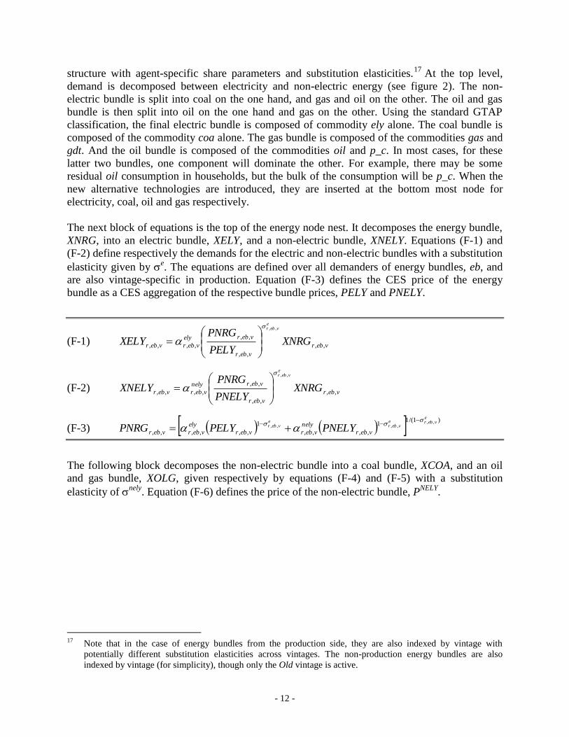
The next block of equations is the top of the energy node nest. It decomposes the energy bundle,
XNRG, into an electric bundle, XELY, and a non-electric bundle, XNELY. Equations (F-1) and
(F-2) define respectively the demands for the electric and non-electric bundles with a substitution
elasticity given by e. The equations are defined over all demanders of energy bundles, eb, and
are also vintage-specific in production. Equation (F-3) defines the CES price of the energy
bundle as a CES aggregation of the respective bundle prices, PELY and PNELY.
(F-1) vebr
vebr
vebrely
vebrvebr XNRGPELY
PNRGXELY
evebr
,,
,,
,,
,,,,
,,
(F-2) vebr
vebr
vebrnely
vebrvebr XNRGPNELY
PNRGXNELY
evebr
,,
,,
,,
,,,,
,,
(F-3) )1/(11
,,,,
1
,,,,,,
,,,,,,
evebre
vebre
vebr
vebr
nely
vebrvebr
ely
vebrvebr PNELYPELYPNRG
The following block decomposes the non-electric bundle into a coal bundle, XCOA, and an oil
and gas bundle, XOLG, given respectively by equations (F-4) and (F-5) with a substitution
elasticity of nely
. Equation (F-6) defines the price of the non-electric bundle, PNELY
.
17
Note that in the case of energy bundles from the production side, they are also indexed by vintage with
potentially different substitution elasticities across vintages. The non-production energy bundles are also
indexed by vintage (for simplicity), though only the Old vintage is active.

- 13 -
(F-4) vebr
vebr
vebrcoa
vebrvebr XNELYPCOA
PNELYXCOA
nelyvebr
,,
,,
,,
,,,,
,,
(F-5) vebr
vebr
vebrolg
vebrvebr XNELYPOLG
PNELYXOLG
nelyvebr
,,
,,
,,
,,,,
,,
(F-6) )1/(11
,,,,
1
,,,,,,
,,,,,,
nelyvebrnely
vebrnely
vebr
vebr
olg
vebrvebr
coa
vebrvebr POLGPCOAPNELY
The third node decomposes the oil and gas bundle into a gas bundle, XGAS, and an oil bundle,
XOIL. Equations (F-7) and (F-8) provide the demand equations for the respective bundles with a
substitution elasticity of olg
. Finally, equation (F-9) describes the price of the oil and gas bundle,
POLG, as a CES aggregation of the gas bundle, PGAS, and the oil bundle, POIL.
(F-7) vebr
vebr
vebrgas
vebrvebr XOLGPGAS
POLGXGAS
olgvebr
,,
,,
,,
,,,,
,,
(F-8) vebr
vebr
vebroil
vebrvebr XOLGPOIL
POLGXOIL
olgvebr
,,
,,
,,
,,,,
,,
(F-9) )1/(11
,,,,
1
,,,,,,
,,,,,,
olgvebrolg
vebrolg
vebr
vebr
oil
vebrvebr
gas
vebrvebr POILPGASPOLG
At this point, the decomposition of fuels is down to four fundamental energy sources—
electricity, coal, gas and oil. In the initial state, with the GTAP data alone, each of the six
energies in GTAP is mapped to these four bundles. Four energy sets are defined: ely, coa, oil and
gas that correspond to a mapping to one of the four types of energy. The GTAP ely sector is
mapped to ely, the GTAP coa sector is mapped to coa, the GTAP gas and gdt sectors are mapped
to gas, and the GTAP oil and p_c sectors are mapped to oil. With the introduction of new
technologies, the set mappings will increase. Thus if there is one electric backstop technology,
say renewables, and designated by elybs, it will be mapped to the ely aggregate electric bundle.

- 14 -
(F-10)
aaeb v
vebra
aaelyr
vebre
vebelyr
elybs
vebelyraaelyr XELYPA
PELYXA
elyvebr
elyvebr
,,
,,
,,1
,,,,,,,,
,,
,,
(F-11)
)1/(11
,,,
,,
,,,,,
,,,,
elyvebrely
vebr
ebaa elye
vebelyr
a
aaelyrelybs
vebelyrvebr
PAPELY
(F-12)
aaeb v
vebra
aacoar
vebre
vebcoar
coabs
vebcoaraacoar XCOAPA
PCOAXA
coavebr
coavebr
,,
,,
,,1
,,,,,,,,
,,
,,
(F-13)
)1/(11
,,,
,,
,,,,,
,,,,
coavebrcoa
vebr
ebaa coae
vebcoar
a
aacoarcoabs
vebcoarvebr
PAPCOA
(F-14)
aaeb v
vebra
aagasr
vebre
vebgasr
gasbs
vebgasraagasr XGASPA
PGASXA
gasvebr
gasvebr
,,
,,
,,1
,,,,,,,,
,,
,,
(F-15)
)1/(11
,,,
,,
,,,,,
,,,,
gasvebrgas
vebr
ebaa gase
vebgasr
a
aagasrgasbs
vebgasrvebr
PAPGAS
(F-16)
aaeb v
vebra
aaoilr
vebre
veboilr
oilbs
veboilraaoilr XOILPA
POILXA
oilvebr
oilvebr
,,
,,
,,1
,,,,,,,,
,,
,,
(F-17)
)1/(11
,,,
,,
,,,,,
,,,,
oilvebroil
vebr
ebaa oile
veboilr
a
aaoilroilbs
veboilrvebr
PAPOIL
Equations (F-10) through (F-17) determine the decomposition of the four basic energy bundles to
their respective Armington volumes. For electricity and coal, with the base data, these equations
are somewhat redundant since the bundles map to only one Armington commodity. Each demand
equation requires a summing over vintages (for only activities), and a summing across eb
indices. In most cases, the eb index maps to one, and only one, agent (aa). In the case of
consumption, however, the energy bundle can exist for each consumed commodity (k), and thus
there can be as many energy decompositions as there are consumer commodities. Each bundle
also allows for energy efficiency improvement, sometimes designated as the autonomous energy
efficiency improvement (AEEI) parameter, which is region, agent, fuel and vintage specific (in
principle). The price equations need a separate mapping from the eb to the aa index, though it is
assumed that the consumer price for a given fuel is uniform across the k commodities (i.e. natural
gas used for heat has the same price as natural gas used for transportation.).

- 15 -
Trade block
Top level Armington
The equations above have determined completely the so-called Armington demand for goods
across all agents, XA, that include activities (a), private or consumer demand (h), and other final
demand (f). The union of these three sets is the set aa. In the standard version of ENVISAGE, all
Armington agents are assumed to have the same preference function for domestic and import
goods.18
It is also assumed that the Armington good, for each commodity i, is homogeneous
across agents, and can therefore be aggregated in volume terms. However, when using the
energy volume data that comes with the GTAP data set, the derived energy prices vary (modestly
in most cases) across agents.19
To maintain the adding up assumption with the price differentials,
a shift parameter is associated with each agent. One could think of this intuitively as a quality
index, so the gasoline consumed by households has a different quality than that consumed in
transportation, where quality differences may simply reflect octane levels.
Equation (T-1) defines aggregate Armington demand, XAT. It is the sum across all agents of their
Armington demand—adjusted by the fixed shift (or quality) parameter, c.20
The agent-specific
Armington price is composed of two components. The first, PA, is formed from the nationally
determined Armington price, PAT, defined below, adjusted by the quality index, c, and
augmented by the user-specific sales tax, Ap
—see equation (T-2). To this is added the emission
tax, emi
, see equation (T-3). The emissions tax is given as a $ amount per unit of emission,
where determines the agent specific level of emissions per unit of demand by agent (aa), per
input (i) and per emission type (em). The emissions rate is multiplied by a global emissions
factor e that allows for the emissions rate to vary in the baseline scenario to achieve a given
global emissions trend.21
In other words is calibrated to base year data and e represents trend
changes in the emissions rate. The model allows for full or partial exemptions using the
parameter —that can also be agent, input and emission specific. For example it is possible to
exempt given sectors or households from paying the emissions tax for specific fuels, say
gasoline. By default, the parameter is set at 1, i.e. there are no exemptions. The emissions tax
can be either set exogenously or be model-derived by imposing an emissions cap at either the
country or regional level.22
Notice that the emission tax is not an ad valorem tax, but a Pigouvian
per unit tax.
18
The GTAP data decomposes Armington demand into its domestic and import component by agent. Annex 3
explains an alternative version of the Armington decomposition that allows for agent-specific behavior. Note
that this increases the size of the model considerably. 19
The energy data, derived from the databases of the International Energy Agency (IEA), are expressed in
millions of tons of oil equivalent (MTOE) across all energies, and thus prices are $2004 prices per unit of
MTOE. 20
The c parameter is initialized at 1 for all non-energy commodities. For energy commodities, it is initialized
such that there is uniformity of energy prices in efficiency units. 21
The baseline calibration of the emission rates only affects non-CO2 greenhouse gases. 22
The model does not include equation (T-3) as it has been substituted throughout to minimize the creation of
additional variables.

- 16 -
(T-1) aa
air
c
aairir XAXAT ,,,,,
(T-2) ir
c
aair
Ap
aairaair PATPA ,,,,,,, )1(
(T-3) , , , , , , , , , , ,
a emi e
r i aa r i aa r em em r em i aa r em i aa
em
PA PA
As described above, the decomposition of the Armington aggregate, XAT, is done at the national
level. (The Armington equations are all indexed by im. The model allows for homogeneous
traded commodities and these are indexed by ih.) Aggregate national demand for domestic
goods, XD, is then a fraction of XAT, with the fraction sensitive to the relative price of domestic
goods, PD, to the Armington good, PAT—as shown in equation (T-4). The key parameter,
known as the Armington substitution elasticity, is m. The model allows for quality differences
in the Armington composite goods using the a and
t parameters. These in effect allow one to
calibrate the CES functions in terms of value shares with the appropriate initialization of the
respective parameters. Equation (T-5) determines the demand for aggregate imports, XMT,
which are further decomposed by trading partner (see below). The price of aggregate imports is
tariff-inclusive. Finally, equation (T-6) defines the aggregate (or national) price of the aggregate
Armington good, PAT.
(T-4) air
imr
imra
imr
d
imrimr XATPD
PATXD
mimr
mimr
,,
,
,1
,,,
,
,
(T-5) air
imr
imrt
imr
m
imrimr XATPMT
PATXMT
mimr
mimr
,,
,
,1
,,,
,
,
(T-6)
)1/(11
,
,
,
1
,
,
,,
,,,,,
mairm
airm
imr
t
imr
imrm
imra
imr
imrd
imrimr
PMTPDPAT
Each bilateral trade flow is associated with four different prices:
1. PE represents the factory or farm gate price
2. WPE represents the FOB price, an export tax or subsidy induces a wedge between the
producer price and the FOB price23
3. WPM represents the CIF price, international trade and transport margins introduce a
wedge between the FOB and CIF price
4. PM represents the agent-price and includes the bilateral tariff
23
The ENVISAGE model specification of export taxes is that they are an ad valorem tax on the producer price,
thus an export subsidy is negative. An alternative formulation would be to specify the tax as a wedge between
the world price and the domestic FOB price in which case the subsidy is measured as a positive wedge.

- 17 -
Equations (T-7) through (T-9) describe three of the prices associated with international trade,
respectively WPE, WPM and PM (the determination of PE is described below). The respective
wedges are represented by e, the export tax/subsidy,
tm, the international transport margin, and
m the bilateral tariff. The price of a unit of international transport is uniform, irrespective of the
transport node and sector.
Second level Armington nest
The second nest in the Armington structure allocates aggregate import demand (across all
agents) to specific regions of origin.24
The bilateral trade flow will reflect preferences, the region
of origin-specific export price and the bilateral tariff, m. The price impacts are reflected in the
tariff-inclusive bilateral price PM. Equation (T-10) defines import demand, WTFd, by region r,
sourced in region r'. Equation (T-11) defines the aggregate import price, PMT. It is an
aggregation of the tariff inclusive bilateral import price. All agents are assumed to face the same
import price (net of the sales tax), i.e. implicitly we are assuming that the composition of the
import bundle by each agent is identical.
(T-7) imrr
e
imrrimrr PEWPE ,',,',,', )1(
(T-8) PWMGWPEWPM tm
imrrimrrimrr ,',,',,',
(T-9) imrr
m
imrrimrr WPMPM ,',,',,', )1(
(T-10) imr
imrr
imrm
imrr
w
imrr
d
imrr XMTPM
PMTWTF
wimr
wimr
,
,,'
,1
,',,',,'
,
,
(T-11)
)1/(1
'
1
,,'
,,'
,,',
,,
wimrw
imr
rm
imrr
imrrw
imrrimr
PMPMT
Export supply
Analogous to the two-nested Armington specification described above, the ENVISAGE model
allows for imperfect transformation of output across markets of destination—domestic and for
export. A two-nested CET structure is implemented. At the top level, output is allocated between
the domestic market and aggregate exports. At the next level, aggregate exports are allocated
across various foreign markets. At either nest, infinite transformation is allowed in which case
the CET first order conditions are replaced by the law of one price. The supply of international
trade and transport services (XMG) is treated apart and is assumed to be priced at the average
producer price, PP.
24
Note that in either version of the top-level Armington decomposition—national or agent-specific—the
decomposition of imports by region of origin is specified at the national level.
- 18 -
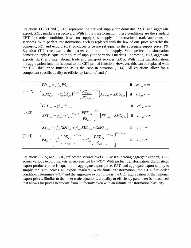
Equations (T-12) and (T-13) represent the derived supply for domestic, XDT, and aggregate
export, XET, markets respectively. With finite transformation, these conditions are the standard
CET first order conditions based on supply (less supply of international trade and transport
services). With perfect transformation, each is replaced with the law of one price whereby the
domestic, PD, and export, PET, producer price are set equal to the aggregate supply price, PS.
Equation (T-14) represents the market equilibrium for supply. With perfect transformation
domestic supply is equal to the sum of supply to the various markets—domestic, XDT, aggregate
exports, XET, and international trade and transport services, XMG. With finite transformation,
the aggregation function is equal to the CET primal function. However, this can be replaced with
the CET dual price function as is the case in equation (T-14). All equations allow for a
component specific quality or efficiency factor, d and
e.
(T-12)
x
imrimrimr
imr
imrd
imr
xd
imr
s
imr
x
imrimr
d
imrimr
XMGXSPS
PDXDT
PSPDx
imrx
imr
,,,
,
,1
,,,
,,,,
if
if
,
,
(T-13)
x
imrimrimr
imr
imre
imr
xe
imrimr
x
imrimr
e
imrimr
XMGXSPS
PETXET
PSPETx
imrx
imr
,,,
,
,1
,,,
,,,,
if
if
,
,
(T-14) ,
, ,
, , , , , , ,
1/(1 )1 1
, ,
, , , ,
, ,
if
if
xr imx x
r im r im
d s e x
r im r im r im r im r im r im r i
r im r imxd xe x
r i r im r im r id e
r im r im
XS XDT XET XMG
PD PETPS
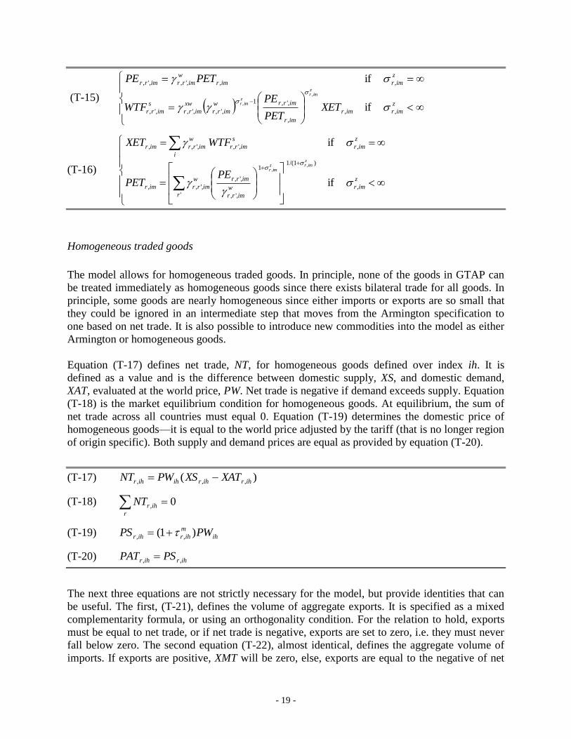
Equations (T-15) and (T-16) reflect the second level CET nest allocating aggregate exports, XET,
across various export markets as represented by WTFs. With perfect transformation, the bilateral
export producer price is equal to the aggregate export price, PET, and aggregate export supply is
simply the sum across all export markets. With finite transformation, the CET first-order
condition determines WTFs and the aggregate export price is the CET aggregation of the regional
export prices. Similar to the other trade equations, a quality or efficiency parameter is introduced
that allows for prices to deviate from uniformity even with an infinite transformation elasticity.
- 19 -
(T-15)
z
imrimr
imr
imrrw
imrr
xw
imrr
s
imrr
z
imrimr
w
imrrimrr
XETPET
PEWTF
PETPEz
imrz
imr
,,
,
,',1
,',,',,',
,,,',,',
if
if
,
,
(T-16)
z
imr
rw
imrr
imrrw
imrrimr
z
imr
i
s
imrr
w
imrrimr
zimrz
imr
PEPET
WTFXET
,
)1/(1
'
1
,',
,',
,',,
,,',,',,
if
if
,,
Homogeneous traded goods
The model allows for homogeneous traded goods. In principle, none of the goods in GTAP can
be treated immediately as homogeneous goods since there exists bilateral trade for all goods. In
principle, some goods are nearly homogeneous since either imports or exports are so small that
they could be ignored in an intermediate step that moves from the Armington specification to
one based on net trade. It is also possible to introduce new commodities into the model as either
Armington or homogeneous goods.
Equation (T-17) defines net trade, NT, for homogeneous goods defined over index ih. It is
defined as a value and is the difference between domestic supply, XS, and domestic demand,
XAT, evaluated at the world price, PW. Net trade is negative if demand exceeds supply. Equation
(T-18) is the market equilibrium condition for homogeneous goods. At equilibrium, the sum of
net trade across all countries must equal 0. Equation (T-19) determines the domestic price of
homogeneous goods—it is equal to the world price adjusted by the tariff (that is no longer region
of origin specific). Both supply and demand prices are equal as provided by equation (T-20).
(T-17) )( ,,, ihrihrihihr XATXSPWNT
(T-18) 0, r
ihrNT
(T-19) ih
m
ihrihr PWPS )1( ,,
(T-20) ihrihr PSPAT ,,
The next three equations are not strictly necessary for the model, but provide identities that can
be useful. The first, (T-21), defines the volume of aggregate exports. It is specified as a mixed
complementarity formula, or using an orthogonality condition. For the relation to hold, exports
must be equal to net trade, or if net trade is negative, exports are set to zero, i.e. they must never
fall below zero. The second equation (T-22), almost identical, defines the aggregate volume of
imports. If exports are positive, XMT will be zero, else, exports are equal to the negative of net
- 20 -
trade and will be positive. The third is a definition of a world price for Armington goods, and is a
weighted global average of domestic supply prices, PS.
(T-21) 0).( ,,, ihrihrihrih XETNTXETPW and 0, ihrXET
(T-22) )( ,,, ihrihrihihr XMTXETPWNT
(T-23) , , , , ,
w
im t r im t r im t
r
PW PS
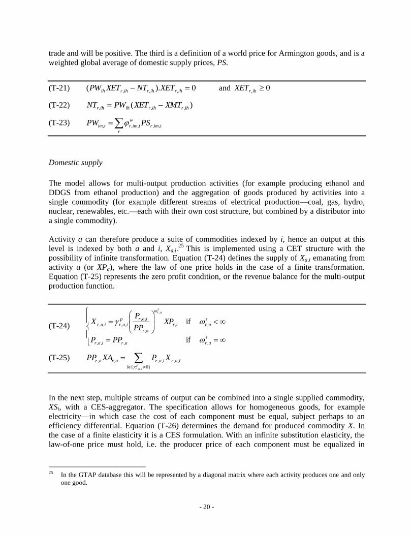
Domestic supply
The model allows for multi-output production activities (for example producing ethanol and
DDGS from ethanol production) and the aggregation of goods produced by activities into a
single commodity (for example different streams of electrical production—coal, gas, hydro,
nuclear, renewables, etc.—each with their own cost structure, but combined by a distributor into
a single commodity).
Activity a can therefore produce a suite of commodities indexed by i, hence an output at this
level is indexed by both a and i, Xa,i.25
This is implemented using a CET structure with the
possibility of infinite transformation. Equation (T-24) defines the supply of Xa,i emanating from
activity a (or XPa), where the law of one price holds in the case of a finite transformation.
Equation (T-25) represents the zero profit condition, or the revenue balance for the multi-output
production function.
(T-24)
s
arariar
s
arir
ar
iarp
iariar
PPP
XPPP
PX
sar
,,,,
,,
,
,,
,,,,
if
if
,
(T-25)
, ,
, , , , , ,
{ 0}pr a i
r a r a r a i r a i
i
PP XA P X
In the next step, multiple streams of output can be combined into a single supplied commodity,
XSi, with a CES-aggregator. The specification allows for homogeneous goods, for example
electricity—in which case the cost of each component must be equal, subject perhaps to an
efficiency differential. Equation (T-26) determines the demand for produced commodity X. In
the case of a finite elasticity it is a CES formulation. With an infinite substitution elasticity, the
law-of-one price must hold, i.e. the producer price of each component must be equalized in
25
In the GTAP database this will be represented by a diagonal matrix where each activity produces one and only
one good.
- 21 -
efficiency units. Equation (T-27) determines the equilibrium condition in the form of the cost
function equality.
(T-26)
s
irir
s
ariar
s
irir
iar
irs
ar
s
iariar
PSP
XSP
PSX
sir
sir
,,,,,
,,
,,
,1
,,,,,
if
if)(
,
,
(T-27)
, ,
, , , , , ,
{ 0}sr a i
r i r i r a i r a i
a
PS XS P X
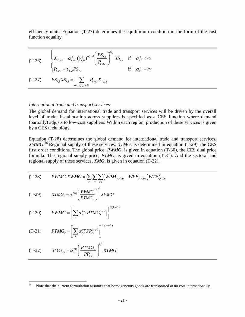
International trade and transport services
The global demand for international trade and transport services will be driven by the overall
level of trade. Its allocation across suppliers is specified as a CES function where demand
(partially) adjusts to low-cost suppliers. Within each region, production of these services is given
by a CES technology.
Equation (T-28) determines the global demand for international trade and transport services,
XWMG.26
Regional supply of these services, XTMG, is determined in equation (T-29), the CES
first order conditions. The global price, PWMG, is given in equation (T-30), the CES dual price
formula. The regional supply price, PTMG, is given in equation (T-31). And the sectoral and
regional supply of these services, XMG, is given in equation (T-32).
(T-28) , ', , ', , ',
'
. s
r r im r r im r r im
r r im
PWMG XWMG WPM WPE WTF
(T-29) XWMGPTMG
PWMGXTMG
t
r
tmgrr
(T-30)
)1/(1
1
t
t
r
r
tmg
r PTMGPWMG
(T-31)
)1/(1
1
,,
rtr
rtr
i
ir
mg
irr PPPTMG
(T-32) r
ir
rmg
irir XTMGPP
PTMGXMG
rtr
,
,,
26
Note that the current formulation assumes that homogeneous goods are transported at no cost internationally.

- 22 -
Product market equilibrium
The model has only two ‘basic’ commodities—domestically produced goods for the domestic
market, XDT, and bilateral exports, WTF. All other goods are composite goods. Equations (E-1)
and (E-2) determine the equilibrium price for these two sets of goods, respectively PD and PE.
With perfect transformation (at both levels), the true goods market equilibrium price is PS and
equation (T-14) is the market equilibrium condition. In the model implementation, the
equilibrium conditions (E-1) and (E-2) are substituted out.
(E-1) sir
dir XDTXDT ,,
(E-2) sirr
dirr WTFWTF ,',,',
Factor market equilibrium
The GTAP database has five factors of production—unskilled and skilled labor, capital, land and
natural resources (or sector-specific factors: forestry, fishing, coal, oil, natural gas and other
mining).27
The next sections describe factor market equilibrium for these factors. The first
describes a resource with a national market—with no, partial or full mobility. In the standard
version of ENVISAGE, this covers only the aggregate land market.28
Labor markets are covered
separately. The model allows for labor market segmentation where the rural and urban markets
clear separately and with the existence of a Harris-Todaro type rural to urban migration function.
Natural resources have a supply curve under various assumptions. Finally, the capital market is
handled apart—partially to implement the vintage capital structure.
Economy-wide factor markets
In the standard version of ENVISAGE land markets are national, i.e. economy-wide markets
ranging from no mobility to full mobility. In the comparative static model, capital markets are
treated the same way, but the dynamic version of the model, with vintage capital, has a
somewhat different structure.
Clearance on national markets is governed by the degree of mobility across sectors and is
modeled using a constant-elasticity-of-transformation specification. With an infinite
transformation elasticity, factors of production are perfectly mobile across sectors and the law of
one price holds. With finite (and even zero) transformation elasticity, factors are only partially
mobile (or sector-specific) and factor returns are sector specific.
Equation (F-1) first determines aggregate national supply, XFT. The index fpn covers all
nationally allocated factors of production—by default just land, and capital in the comparative
static version of the model. There are two specification—either a constant elasticity specification
27
GTAP also includes an additional satellite account that divides the land resource into 18 agro-ecological land
types (AEZs). These have not been integrated in the standard version of ENVISAGE but have been
implemented in a specialized version focused on bio-fuels (see Beghin et al 2010 [to be checked]). 28
In the comparative static version of the model, it also is used for capital allocation.
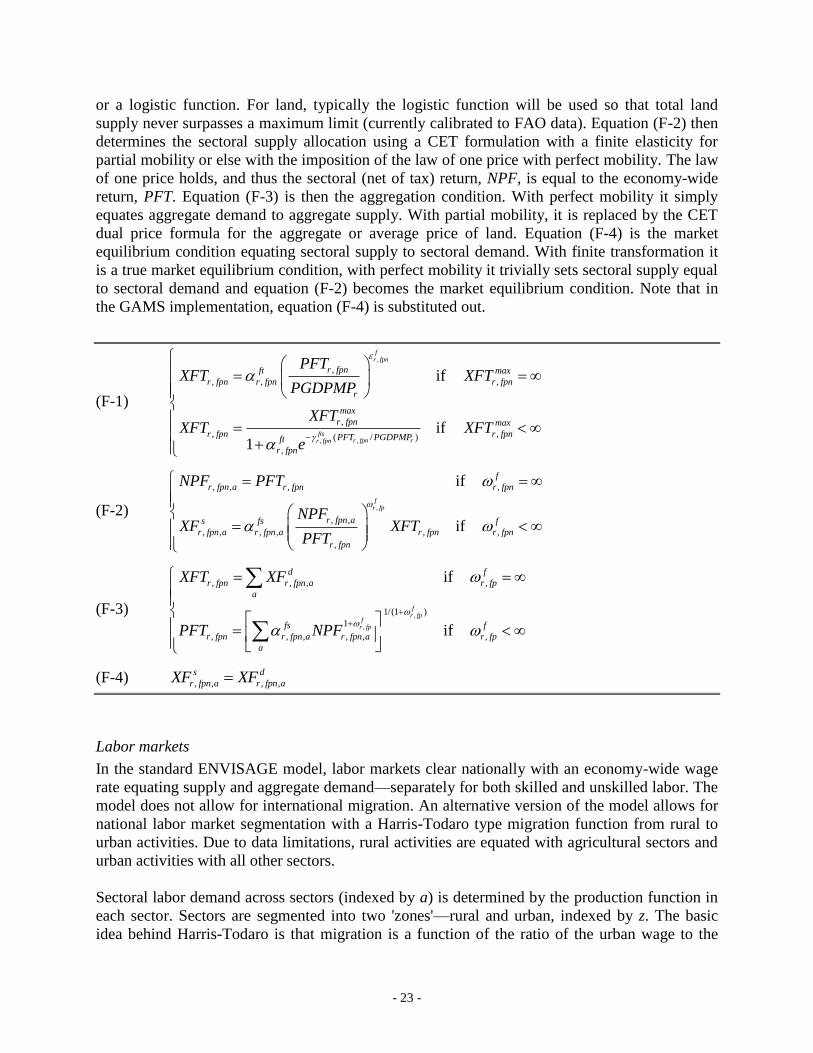
- 23 -
or a logistic function. For land, typically the logistic function will be used so that total land
supply never surpasses a maximum limit (currently calibrated to FAO data). Equation (F-2) then
determines the sectoral supply allocation using a CET formulation with a finite elasticity for
partial mobility or else with the imposition of the law of one price with perfect mobility. The law
of one price holds, and thus the sectoral (net of tax) return, NPF, is equal to the economy-wide
return, PFT. Equation (F-3) is then the aggregation condition. With perfect mobility it simply
equates aggregate demand to aggregate supply. With partial mobility, it is replaced by the CET
dual price formula for the aggregate or average price of land. Equation (F-4) is the market
equilibrium condition equating sectoral supply to sectoral demand. With finite transformation it
is a true market equilibrium condition, with perfect mobility it trivially sets sectoral supply equal
to sectoral demand and equation (F-2) becomes the market equilibrium condition. Note that in
the GAMS implementation, equation (F-4) is substituted out.
(F-1)
,
,,
,
, , ,
,
, ,( / )
,
if
if1
fr fpn
ftsr fpn rr fpn
r fpnft max
r fpn r fpn r fpn
r
max
r fpn max
r fpn r fpnPFT PGDPMPft
r fpn
PFTXFT XFT
PGDPMP
XFTXFT XFT
e
(F-2) ,
, , , ,
, ,
, , , , , ,
,
if
if
fr fp
f
r fpn a r fpn r fpn
r fpn as fs f
r fpn a r fpn a r fpn r fpn
r fpn
NPF PFT
NPFXF XFT
PFT
(F-3) ,
,
, , , ,
1/(1 )
1
, , , , , ,
if
if
fr fp
fr fp
d f
r fpn r fpn a r fp
a
fs f
r fpn r fpn a r fpn a r fp
a
XFT XF
PFT NPF
(F-4) , , , ,
s d
r fpn a r fpn aXF XF
Labor markets
In the standard ENVISAGE model, labor markets clear nationally with an economy-wide wage
rate equating supply and aggregate demand—separately for both skilled and unskilled labor. The
model does not allow for international migration. An alternative version of the model allows for
national labor market segmentation with a Harris-Todaro type migration function from rural to
urban activities. Due to data limitations, rural activities are equated with agricultural sectors and
urban activities with all other sectors.
Sectoral labor demand across sectors (indexed by a) is determined by the production function in
each sector. Sectors are segmented into two 'zones'—rural and urban, indexed by z. The basic
idea behind Harris-Todaro is that migration is a function of the ratio of the urban wage to the
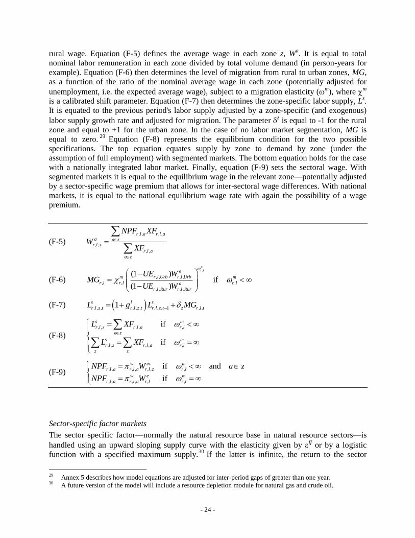
- 24 -
rural wage. Equation (F-5) defines the average wage in each zone z, Wa. It is equal to total
nominal labor remuneration in each zone divided by total volume demand (in person-years for
example). Equation (F-6) then determines the level of migration from rural to urban zones, MG,
as a function of the ratio of the nominal average wage in each zone (potentially adjusted for
unemployment, i.e. the expected average wage), subject to a migration elasticity (m), where
m
is a calibrated shift parameter. Equation (F-7) then determines the zone-specific labor supply, Ls.
It is equated to the previous period's labor supply adjusted by a zone-specific (and exogenous)
labor supply growth rate and adjusted for migration. The parameter z is equal to -1 for the rural
zone and equal to +1 for the urban zone. In the case of no labor market segmentation, MG is
equal to zero.29
Equation (F-8) represents the equilibrium condition for the two possible
specifications. The top equation equates supply by zone to demand by zone (under the
assumption of full employment) with segmented markets. The bottom equation holds for the case
with a nationally integrated labor market. Finally, equation (F-9) sets the sectoral wage. With
segmented markets it is equal to the equilibrium wage in the relevant zone—potentially adjusted
by a sector-specific wage premium that allows for inter-sectoral wage differences. With national
markets, it is equal to the national equilibrium wage rate with again the possibility of a wage
premium.
(F-5) , , , ,
, ,
, ,
r l a r l aa a z
r l z
r l a
a z
NPF XF
WXF
(F-6)
,
, , , ,
, , ,
, , , ,
(1 )if
(1 )
mr la
r l Urb r l Urbm m
r l r l r la
r l Rur r l Rur
UE WMG
UE W
(F-7) , , , , , , , , , 1 , ,1s l s
r l z t r l z t r l z t z r l tL g L MG
(F-8) , , , , ,
, , , , ,
if
if
s m
r l z r l a r l
a z
s m
r l z r l a r l
z z
L XF
L XF
(F-9) , , , , , , ,
, , , , , ,
if and
if
w ez m
r l a r l a r l z r l
w e m
r l a r l a r l r l
NPF W a z
NPF W
Sector-specific factor markets
The sector specific factor—normally the natural resource base in natural resource sectors—is
handled using an upward sloping supply curve with the elasticity given by ff or by a logistic
function with a specified maximum supply.30
If the latter is infinite, the return to the sector
29
Annex 5 describes how model equations are adjusted for inter-period gaps of greater than one year. 30
A future version of the model will include a resource depletion module for natural gas and crude oil.

- 25 -
specific factor is assumed to rise at the same rate as the GDP deflator, see equation (F-11), else it
is determined by market equilibrium. The finite supply curve has three shifters. The first, fs, is
calibrated with base year data. The second, rfs
, can be calibrated in a dynamic scenario to target
a region specific variable, for example output or the regional producer price. The third, gfs
, can
be calibrated in a dynamic scenario to target a global variable, for example global output or the
global price. In this case, the shifter moves each country/regional supply curve by the same
proportional amount.
(F-10)
,
, , ,
, ,
, , , , ,
,
, , ,( / )
, ,
if and
if and1
ffr a
fsr a r NatRs a r
r NatRs as rfs gfs fs ff max
r a r a a r a r a r a
r
max
r as ff max
r a r a r aNPF PGDPMPfs
r NatRs a
NPFXF XF
PGDPMP
XFXF XF
e
(F-11) , , , ,
, , , , , , 1 ,
if
. if
s ff
r a r NatRs a r a
ff
r NatRs a t r r NatRs a t r a
XF XF
NPF PGDPMP NPF
Capital markets with the vintage capital specification
This section describes sectoral capital allocation under the assumption of multiple vintage
capital. Capital market equilibrium under the vintage capital framework assumes the following:
New capital is perfectly mobile and its allocation across sectors insures a
uniform rate of return.
Old capital in expanding sectors is equated to new capital, i.e. the rate of
return on Old capital in expanding sectors is the same as the economy-wide
rate of return on new capital.
Declining sectors release Old capital. The released Old capital is added to the
stock of New capital. The assumption here is that declining sectors will first
release the most mobile types of capital, and this capital, being mobile, is
comparable to New capital (e.g. transportation equipment).
The rate of return on capital in declining sectors is determined by sector-
specific supply and demand conditions.
The result of these assumptions is that if there are no sectors with declining economic activity,
there is a single economy-wide rate of return. In the case of declining sectors, there will be an
additional sector-specific rate of return on Old capital for each sector in decline.
To determine whether a sector is in decline or not, one assesses total sectoral demand (which of
course, in equilibrium equals output). Given the capital-output ratio, it is possible to calculate
whether the initially installed capital is able to produce the given demand. In a declining sector,
the installed capital will exceed the capital necessary to produce existing demand. These sectors
will therefore release capital on the secondary capital market in order to match their effective

- 26 -
(capital) demand with supply. The supply schedule for released capital is a constant elasticity of
supply function where the main argument is the change in the relative return between Old and
New capital. Supply of capital to the declining sector is given by the following formula:
ki
NewaOldaa
s
Olda RRKK
,,
0
, /
where KsOld is capital supply in the declining sector, K
0 is the initial installed (and depreciated)
capital in the sector at the beginning of the period, and k is the dis-investment elasticity. (Note
that in the model, the variable R is represented by PF.) In other words, as the rate of return on
Old capital increases towards (decreases from) the rate of return on New capital, capital supply in
the declining sector will increase (decrease). Released capital is the difference between K0 and
Ks,Old
. It is added to the stock of New capital. In equilibrium, the Old supply of capital must equal
the sectoral demand for capital:
Olda
s
Olda KVK ,,
Inserting this into the equation above and defining the following variable
NewaOldaa RRRR ,, /
yields the following equilibrium condition:
ka
aaOlda RRKKV0
,
The supply curve is kinked, i.e. the relative rate of return is bounded above by 1. If demand for
capital exceeds installed capital, the sector will demand New capital and the rate of return on Old
capital is equal to the rate of return on New capital, i.e. the relative rate of return is 1. The kinked
supply curve has been transformed into a mixed complementarity (MCP) relation. The following
inequality is inserted in the model:
a
v
a
Notd
aaa
s
Olda XPKRRKKka
,0
,
The right-hand side determines the notional demand for capital in sector a, i.e. it assesses
aggregate output (equal to demand) and multiplies this by the capital output ratio for Old capital.
This is then the derived demand for Old capital. If the installed capital is insufficient to meet
demand for Old capital, the sector will demand New capital, and the inequality obtains with the
relative rates of return capped at 1. If the derived demand for Old capital is less than installed
capital, the sector will release capital according to the supply schedule. In this case the inequality
transforms into an equality, and the relative rate of return is less than 1.
Equation (F-12) determines the capital output ratio, v for Old capital. Equation (F-13) specifies
the supply schedule of Old capital. In effect, this equation determines the variable RR, the
relative rate of return between Old and New capital.

- 27 -
(F-12) Oldar
Oldarv
arXPv
KV
,,
,,
,
(F-13) 1and ,,,,
0
, arar
v
ararar RRXPRRKki
There is a single economy-wide rate of return on New capital. The equilibrium rate of return on
New capital is determined by setting aggregate supply equal to aggregate demand. Aggregate
demand for new capital is given by:
Expandinga v
vaKV ,
where the set Expanding includes all sectors in expansion. Since Old capital in expanding sectors
is equated with New capital, the appropriate sum is over all vintages. The aggregate capital stock
of New capital is equal to the total capital stock, less capital supply in declining sectors:
Declininga
Olds
a
s KK ,
where the set Declining covers only those sectors in decline. However, at equilibrium, capital
supply in declining sectors must equal capital demand for Old capital, and capital demand for
New capital in these sectors is equal to zero. Hence, the supply of Old capital in declining sectors
can be shifted to the demand side of the equilibrium condition for New capital, and this
simplification yields equation (F-14) which determines the economy-wide rate of return on New
capital. Equation (F-15) adds up capital demand across vintages. Equation (F-16) determines the
vintage and sector specific rates of return.31
For New capital, RR is 1 and thus the rate of return
on New capital is always equal to the economy-wide rate of return (adjusted by the factor tax).
For Old capital, if the sector is in decline, RR is less than 1 and the rate of return on Old capital
will be less than the economy-wide rate of return (adjusted by the factor tax).
(F-14) v
varaCaptlr KVXF ,,,,
(F-15) Captlr
a
aCaptlr XFTXF ,,,
(F-16) )1( ,,,,,,
v
aCaptlrarCaptlrvar RRPFTPKV
Allocation of Output across Vintages
This section describes how output is allocated across vintages. Aggregate sectoral output, XP, is
equated to aggregate sectoral demand and is derived from XS, which itself is derived from a CET
aggregation of XD and XET. Given the beginning of period installed capital, it is possible to
assess the level of potential output produced using the installed capital. If this level of output is
31
These are the net rates of return after tax. Thus the relative rate of return variable, RR, is defined in terms of the
net rate of return.

- 28 -
greater than the aggregate output (demand) level, the sector appears to be in decline, installed
capital will be released, Old output will be equated with aggregate output (demand), and New
output is zero. Equation (F-17) equates aggregate output, XP, to the sum of output across all
vintages. Equation (F-18) determines output that can be derived from installed, or Old capital,
thus equation (F-17) in essence determines output produced with New capital by residual. Old
output is equated to the sectoral supply of Old capital, divided by the capital/output ratio. The
final two equations are necessary price identities. Equation (F-19) sets the aggregate price of
capital—in both declining and expanding sectors it is equal to the rate of return on Old capital.
Equation (F-20) links the user-price of all factors of production to the after-tax sectoral price of
each of the factors.
(F-17) a
varar XPvXP ,,,
(F-18) v
arararOldar
kiRRKXPv ,,
0
,,, /
(F-19) OldaraCaptlr PKVPF ,,,,
(F-20) afpr
v
afprafpr NPFPF ,,,,,, )1(
Macro closure
Equation (M-1) defines the government accounting balance, Sg. It is the difference between
revenues and expenditures, the latter including some share of stock-building expenditures.
Equation (M-2) defines real government savings. Real government savings are fixed—to insure
at the least debt sustainability. Nominal revenues are endogenous. The direct tax schedule shifts
to achieve the given fiscal target (using the k shifter). Equation (M-3) defines foreign savings, S
f.
These are fixed in numéraire terms for all regions save a residual region (indexed by rSav).
Equation (M-4) insures capital flow equilibrium at the global level (and in effect defines foreign
savings for the residual region).32
Equation (M-5) defines the depreciation allowance. Equation
(M-6) represents the investment/savings balance, with aggregate gross investment expenditures
on the left-side and total available savings on the right, including the depreciation allowance and
adjusted for stock-building expenditures. The model’s price anchor, or numéraire, PNUM, is
defined in equation (M-7). It is defined as the unit value of manufactured exports from the high-
income countries, where the set defined by Numer spans the manufactured sectors. One equation
needs to be dropped from the model specification and typically one equation from equation (M-
6) is dropped. This in fact represents a global Walras’ Law that has global investment equal to
global savings.
32
Alternative versions of the model allow for partial mobility of global savings. These are described in Annex 4.

- 29 -
(M-1) i
stbirstbir
stb
GovrGovrGovrr
g
r XAPAXCPCYGS ,,,,,,,
(M-2) /g
r r rRSg S PGDPMP
(M-3) . forffrrS S PNUM r rSav
(M-4) 0f
r
r
S
(M-5) trInvrrr KPCDeprY ,,
(M-6) , , , , , , , ,
h g f stb
r Inv r Inv r h r r r r Inv r i stb r i stb
h i
PC XC S S S DeprY PA XA
(M-7) , ', , ',
'
n
r r i r r i
r HIC r i Numer
PNUM WPE
The following block of equations provides the main macroeconomic identities. Equations (M-8)
and (M-9) represent nominal and real GDP at market price, GDPMP and RGDPMP respectively.
The GDP at market price deflator, PGDPMP, is defined in equation (M-10). Per capita real
output, RGDPPC, is defined in equation (M-11). Equation (M-12) defines real per capita income
growth. And the GDP absorption shares, GDPShr, are provided in equation (M-13). Equation
(M-14) defines real domestic absorption—it is the sum of household, government and
investment real expenditures.
The default closure rules of the model are as follows:
Household savings are endogenous and are either driven by the demographic-influenced
savings function or as part of the ELES consumer demand system.33
Government revenues are endogenous and government expenditures, as a share of
nominal GDP, are fixed, thus total expenditures are endogenous. The government balance
is fixed, in part to avoid problems of financing sustainability. The government balance is
achieved with a uniform shift in the household direct tax schedule. This implies that new
revenues, for example generated by a carbon tax, would lower direct taxes paid by
households.
Investment is savings driven. Household and government savings were discussed above.
Foreign savings, in the default closure are fixed. Thus investment is largely influenced
through household savings.34
33
The latter may allow for demographics and other factors to influence the ELES parameters between periods in
the dynamic setting where ELES parameters may be re-calibrated. 34
Alternative closures are conceivable, for example targeting investment (as a share of GDP) and allowing the
household savings schedule adjust to achieve the target.

- 30 -
The current account, the mirror entry of the capital account, is exogenous. Ex ante
changes to trade, for example a rise in the world price of imported oil, is met through ex
post changes in the real exchange rate.
(M-8)
'
,,',,',',,',
,,,,,,,,,
.r i
rrimrrimrrimrrimrr
ih
ihr
i
stbirstbir
in
inirinirr
XTMGPTMGWTFWPMWTFWPE
NTXAPAXAPAGDPMP
(M-9)
rrihrihr
ih
ih
r i
imrrimrrimrrimrr
i
stbirstbir
in
inirinirr
XTMGPTMGXMTXETPW
WTFWPMWTFWPE
XAPAXAPARGDPMP
.)( 0,0,,,0,
'
,,'0,,,',',0,,',
,,0,,,,,0,,,
(M-10) rrr RGDPMPGDPMPPGDPMP /
(M-11) rrr PopRGDPMPRGDPPC /
(M-12)
1/
,
,
,
1
n
r typc
r t
r t n
RGDPPCg
RGDPPC
(M-13) r
inrinr
inrGDPMP
XCPCGDPShr
,,
,
(M-14) , , ,0 , ,r t r in r in t
in
RYD PC XC
Model Dynamics
Model dynamics are driven by three factors—similar to most neo-classical growth models.
Population and labor force growth rates are exogenous and given essentially by the UN
Population Division scenario. The labor force growth rate is equated to the growth rate of the
working age population, i.e. the population aged between 15 and 64.35
The second factor is capital accumulation. The aggregate capital stock in any given year, KStock,
is equated to the previous year capital stock, less depreciation at a rate of , plus the previous
period’s volume of investment, XCInv, see equation (G-1). The latter is influenced by the national
savings rate plus foreign savings and, as well, the unit cost of investment. The aggregate capital
stock variable takes two forms. The first, KStock, is the aggregate capital stock evaluated at
$2004 prices. The second is the ‘normalized’ aggregate capital stock, XFT. The normalized
35
In future work, these assumptions will be linked to other variables influencing both the decision to work (i.e. the
labor force participation rate) and the skill level (via assumptions on education).
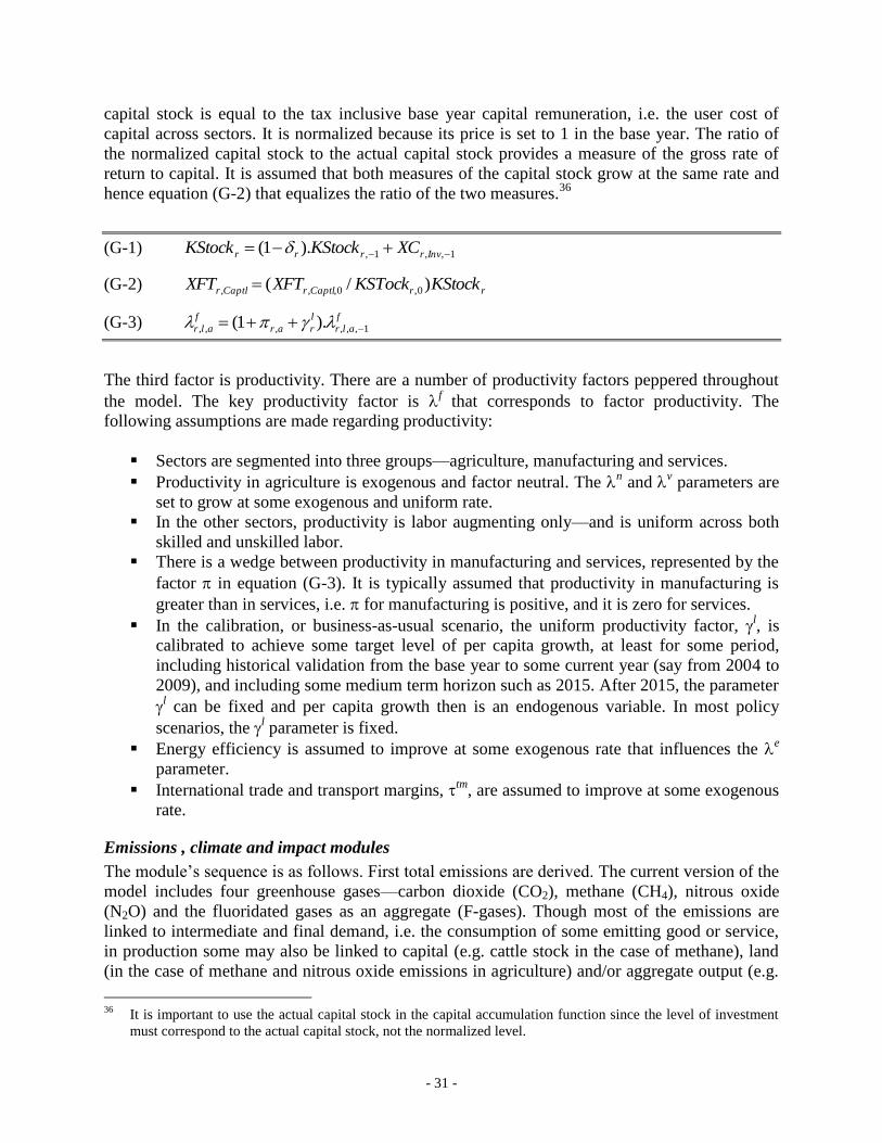
- 31 -
capital stock is equal to the tax inclusive base year capital remuneration, i.e. the user cost of
capital across sectors. It is normalized because its price is set to 1 in the base year. The ratio of
the normalized capital stock to the actual capital stock provides a measure of the gross rate of
return to capital. It is assumed that both measures of the capital stock grow at the same rate and
hence equation (G-2) that equalizes the ratio of the two measures.36
(G-1) 1,,1,).1( Invrrrr XCKStockKStock
(G-2) rrCaptlrCaptlr KStockKSTockXFTXFT )/( 0,0,,,
(G-3) f
alr
l
rar
f
alr 1,,,,,, ).1(
The third factor is productivity. There are a number of productivity factors peppered throughout
the model. The key productivity factor is f that corresponds to factor productivity. The
following assumptions are made regarding productivity:
Sectors are segmented into three groups—agriculture, manufacturing and services.
Productivity in agriculture is exogenous and factor neutral. The n and
v parameters are
set to grow at some exogenous and uniform rate.
In the other sectors, productivity is labor augmenting only—and is uniform across both
skilled and unskilled labor.
There is a wedge between productivity in manufacturing and services, represented by the
factor in equation (G-3). It is typically assumed that productivity in manufacturing is
greater than in services, i.e. for manufacturing is positive, and it is zero for services.
In the calibration, or business-as-usual scenario, the uniform productivity factor, l, is
calibrated to achieve some target level of per capita growth, at least for some period,
including historical validation from the base year to some current year (say from 2004 to
2009), and including some medium term horizon such as 2015. After 2015, the parameter
l can be fixed and per capita growth then is an endogenous variable. In most policy
scenarios, the l parameter is fixed.
Energy efficiency is assumed to improve at some exogenous rate that influences the e
parameter.
International trade and transport margins, tm
, are assumed to improve at some exogenous
rate.
Emissions , climate and impact modules
The module’s sequence is as follows. First total emissions are derived. The current version of the
model includes four greenhouse gases—carbon dioxide (CO2), methane (CH4), nitrous oxide
(N2O) and the fluoridated gases as an aggregate (F-gases). Though most of the emissions are
linked to intermediate and final demand, i.e. the consumption of some emitting good or service,
in production some may also be linked to capital (e.g. cattle stock in the case of methane), land
(in the case of methane and nitrous oxide emissions in agriculture) and/or aggregate output (e.g.
36
It is important to use the actual capital stock in the capital accumulation function since the level of investment
must correspond to the actual capital stock, not the normalized level.

- 32 -
municipal waste-base methane emissions). The emissions of greenhouse gases lead to
atmospheric concentrations—emissions directly add to the atmosphere, but concentrations in the
atmosphere also interact with the ocean and land, creating a dynamic process that would
continue even in the absence of emissions. The atmospheric concentration has an impact on
radiative forcing, i.e. how much of the sun’s energy is reflected back to space. Finally, there is a
set of equations that links radiative forcing to temperature global mean temperature change. The
final phase of the module links changes in the average mean temperature to economic impacts
that feed back into production and demand thereby closing the loop between economic activities,
climate, back to economic activities.
Greenhouse gas emissions
The first emissions equation, equation (C-1), determines the level of emissions, EMI, of type em
for each unit of consumption of commodity i by agent aa, where aa covers all production
activities and final demand accounts. It is simply a fixed coefficient with respect to the demand
level. The emissions rate, , can be adjusted in the baseline by the factor to allow for
autonomous improvements in the emission rates.37
Equation(C-2) captures emissions linked to
the use of factors of production such as capital and/or land. Equation (C-3) are emissions linked
to generic production activities and not to a specific technology, i.e. they are simply output based
emissions. The aggregate emission by region (or country r), EMITot, is defined in equation (C-4)
and is the double sum over all agents and sources (consumption, factor use and production level),
with the possibility of an additional exogenous level of emissions, EMIOth. The level of global
emissions, EMIGbl, is the summation across all countries and regions, with an additional
exogenous component not accounted for in the regional models—see equation (C-5).
(C-1) , , , , , , , ,
e
r em i aa em r em i aa r i aaEMI XA
(C-2) , , , , , , , ,
e
r em fp a em r em fp a r fp aEMI XF
(C-3) , , , , , , ,
e
r em Total a em r em Total a r aEMI XP
(C-4) , , , , ,r em r em is aa r em
aa is
EMITot EMI EMIOth
(C-5) ,em r em em
r
EMIGbl EMITot EMIOthGbl
Emission taxes, caps and trade
There are a number of different potential regimes to limit carbon emissions. The simplest is
simply to impose a carbon tax, i.e. set the variable emi
to some value (measured as $2004 per
unit of emitted C). Emission caps can be set on either a single region/country basis, with a
differentiated carbon tax across regions/countries, or on a region-wide basis with a uniform
37
This has only been used to calibrate the emissions rate of non-CO2 greenhouse gases.

- 33 -
carbon tax. Quota regions are indexed by rq and can be assigned one or more countries.
Examples of cap and cap and trade scenarios are provided in Annex 7. Equation (C-6)
implements emissions caps for each coalition of regions subject to a cap (potentially just a single
country). The sum of emissions across all regions belong to region rq is capped to EMICap (the
shifter is explained below). Equation (C-6) determines the regional emissions tax, emiR
, which
will be uniform across all countries/regions belonging to the coalition region. Equation (C-7)
then is an accounting identity that equates the country/region tax, emi
, to the region-wide
emissions tax.
(C-6)
rqr
emrq
Cap
ememr EMICapEMITot ,,
(C-7) emiR
emrq
emi
emr ,,
(C-8) emremr
emi
emr
emi
emr EMITotEMIQuotaQuotaY ,,,, if Cap and Trade is active
The shifter in equation (C-6) allows for additional targeting, for example a cap on global
emissions. Say for example one wants to cap global emissions by 20 percent but only impose a
cap on Annex I emissions. There is some potential leakage from the cap on Annex I countries—
with non-Annex I countries increasing their emissions—because the world price of fossil fuels
may decline and because they increase their production of carbon intensive goods for export to
the now less competitive Annex I markets. The cap on Annex I countries can then be thought of
as setting the burden shares across Annex I countries and the shifter, Cap
, in equation (C-6) is
then endogenous to meet the overall objective, for example capping global emissions.
Equation (C-8) determines the value of the trade in emissions quota when country/region specific
quotas, EMIQuota, are allocated. The value of the quota is the difference between the quota and
actual emissions, EMITot, valued at the emissions tax level. Currently, it is assumed that the
quota rents are recycled back to the government.
Concentration, forcing and temperature
The current version of ENVISAGE uses a highly simplified climate module that is largely
inspired by the climate module in the MERGE model.38
It replaces the original climate module
that was based on Nordhaus' DICE 2007 model39
because the latter has a CO2-only focus and
ENVISAGE needed a module that could handle other greenhouse gases. We may eventually also
assess the implementation of the PAGE09 climate module that has the added advantage of
providing spatially distinct temperature change in part linked to regional differences in latitude.40
Greenhouse gases are treated differently in their impacts on temperature. Carbon emissions are
released into the atmosphere that is divided into five boxes, Box, indexed by b. New emissions
38
As described in Manne et al 1995 and implemented in the GAMS version of MERGE [need to check source of
code and updates]. 39
Nordhaus 2008, also described in greater detail in Annex 6. 40
Hope 2010.
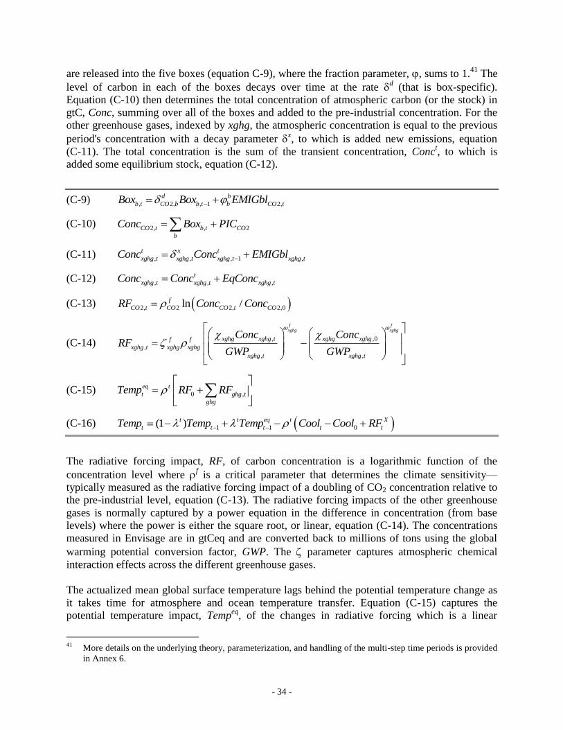
- 34 -
are released into the five boxes (equation C-9), where the fraction parameter, , sums to 1.41
The
level of carbon in each of the boxes decays over time at the rate d (that is box-specific).
Equation (C-10) then determines the total concentration of atmospheric carbon (or the stock) in
gtC, Conc, summing over all of the boxes and added to the pre-industrial concentration. For the
other greenhouse gases, indexed by xghg, the atmospheric concentration is equal to the previous
period's concentration with a decay parameter x, to which is added new emissions, equation
(C-11). The total concentration is the sum of the transient concentration, Conct, to which is
added some equilibrium stock, equation (C-12).
(C-9) , 2, , 1 2,
d b
b t CO b b t b CO tBox Box EMIGbl
(C-10) 2, , 2CO t b t CO
b
Conc Box PIC
(C-11) , , , 1 ,
t x t
xghg t xghg t xghg t xghg tConc Conc EMIGbl
(C-12) , , ,
t
xghg t xghg t xghg tConc Conc EqConc
(C-13) 2, 2 2, 2,0ln /f
CO t CO CO t CORF Conc Conc
(C-14) , ,0
,
, ,
f fxghg xghg
xghg xghg t xghg xghgf f
xghg t xghg xghg
xghg t xghg t
Conc ConcRF
GWP GWP
(C-15) 0 ,
eq t
t ghg t
ghg
Temp RF RF
(C-16) 1 1 0(1 )t t eq t X
t t t t tTemp Temp Temp Cool Cool RF
The radiative forcing impact, RF, of carbon concentration is a logarithmic function of the
concentration level where f is a critical parameter that determines the climate sensitivity—
typically measured as the radiative forcing impact of a doubling of CO2 concentration relative to
the pre-industrial level, equation (C-13). The radiative forcing impacts of the other greenhouse
gases is normally captured by a power equation in the difference in concentration (from base
levels) where the power is either the square root, or linear, equation (C-14). The concentrations
measured in Envisage are in gtCeq and are converted back to millions of tons using the global
warming potential conversion factor, GWP. The parameter captures atmospheric chemical
interaction effects across the different greenhouse gases.
The actualized mean global surface temperature lags behind the potential temperature change as
it takes time for atmosphere and ocean temperature transfer. Equation (C-15) captures the
potential temperature impact, Tempeq
, of the changes in radiative forcing which is a linear
41
More details on the underlying theory, parameterization, and handling of the multi-step time periods is provided
in Annex 6.

- 35 -
function of the aggregate change in radiative forcing. The actual change in temperature, Temp, is
a weighted average of the previous temperature change and the potential temperature—with
potential adjustments due to exogenous cooling and radiative forcing (e.g. sulfates), equation
(C-16).
Climate change economic impacts
The incorporation of climate-related impacts in models of climate change has largely been
relegated to highly aggregate economic models (Nordhaus 1994, 2001 and 2008, Hope 2006)
using a macro damage function that link changes in temperature to a percentage impact on
productivity—normally with an assumption of non-linearity. Hope's damages were initially split
into three distinct impacts—macroeconomic, non economic (such as eco-systems), and a third
damage linked to a sudden discontinuity that could happen after a given temperature threshold.
Hope 2010 has added a fourth channel that splits the impact of sea level rise from the
macroeconomic damage function. Nordhaus 2010 has similarly split his macroeconomic damage
function into two components with sea level rise split from the rest of the impacts.42
The FUND
model (Anthoff and Tol 2008) is also a macro model, but they have vastly extended the impact
side to include agriculture, forestry, water resources, energy consumption, sea level rise, eco-
systems, human health and extreme weather. The initial version of ENVISAGE only
incorporated agricultural damages—calibrated to estimates in Cline 2007, but this limited impact
has been superseded by a new and more complete set of impact estimates and described below.43
Impacts are based on a 2-dimensional table of impact sources and impact destinations. The
impact sources take into account the following:
sea Sea level rise
agr Agricultural productivity
wat Water availability
onj On the job (labor) productivity
tou Tourism
hhe Human health44
end Energy demand
The following impact destinations are considered:
42
The critical part of sea level rise is that the lagged structure of temperature exchange between the atmosphere
and the sea is unusually long so that even if atmospheric temperature rise is reduced relatively rapidly, the
impact on sea level rise would take centuries to dissipate. 43
Much of the remainder of this section is based on Roson 2009. 44
At the moment, the human health component only reflects the direct effect on labor productivity, and not the
increased demand for health services.

- 36 -
lp Labor productivity (or stock)
kp Capital productivity (or stock)
tp Land productivity (or stock)
mp Multi-factor productivity
hc Household consumption of energy
hcser Household consumption of market services
incab Income from abroad
The bulk of the impacts are assumed to be linear with respect to temperature change and are
summarized by equation (C-17), where ddam is the specific damage function by source and
destination. It is implemented as a deviation from the no-damage situation, where ddam takes the
value of 1 in the absence of climate change. A quadratic damage function is used in the case of
agriculture—affecting multi-factor productivity, as depicted in equation (C-18). The following
set of equations implements the damages directly on the relevant model variables. Equation (C-
19) implements the (quadratic) damage on the top-level productivity parameter in the crop
sectors, i.e. it is a uniform shift in the production possibilities frontier across all inputs. It enters
in equations (P-1) through (P-3).45
The next set of four equations determines the impacts on the
factors of production in efficiency units. Equations (C-20) through (C-22) determine the
cumulative impact on respectively labor, land and capital. The standard productivity factors, f,
are determined in the dynamics module, and the climate-impact adjusted parameters, gf
, enter
the production functions. Equation (C-23) is a simple identity as, for the moment, it is assumed
that climate change does not have an impact on the availability of natural resources (i.e. fossil
fuels).
Equation (C-24) represents the impact on household demand. The impact is assumed to affect the
minimal subsistence bundle as represented by the parameter. The impact parameter is
calibrated to the impact on overall consumption, hence the impact on the subsistence level is
scaled for the share of the subsistence level in the overall level of consumption (per capita).
Finally, equation (C-25) represents the impact on tourism revenues, iit. This is a linear function
of the temperature change, where iit0 represents base year tourism revenues. Tourism revenues
accrue to households and this requires a change to equation (Y-10).46
Parametrization of the damage functions is described in Annex 8.
45
The parameters of the damage function are region specific and reflect to some extent the base year structure of
agricultural production, however, the damage as currently formulated applies uniformly across all crop sectors. 46
Similar to all variables that deal with households, the income is allocated across households using the iit
allocation vector—but for the moment, ENVISAGE has only a single representative household and thus the
parameter has unit value.

- 37 -
(C-17) , , , , , , 01 forccd
r src dst t r src dst t tddam T T src Linear
(C-18) 21 2 3
, , , 0 0 01 min(1, )a a a
r agr mp t r t r t r tddam T T T T T T
(C-19) , , ,
cd
r cr r agr mpddam
(C-20) , , , , , ,
gf f
r l a r l a r src lp
src
ddam
(C-21) , , , , , ,
gf f
r LandR a r LandR a r src tp
src
ddam
(C-22) , , , , , ,
gf f
r Captl a r Captl a r src kp
src
ddam
(C-23) , , , ,
gf f
r natrs a r natrs a
(C-24)
, , , ,
, , , ,
, , , , ,0 , ,0
( ) 11
/ /
h
r end hc r k hgh h
r k h r k h h
r k h r k h r h
ddam sign
HX Pop
(C-25) , , ,0 0
iit
r h r h r tiit iit T T

- 38 -
References
Anthoff, David and Richard S. J. Tol (2008), “The Climate Framework for Uncertainty,
Negotiation and Distribution (FUND), Technical Description, Version 3.3,” mimeo, July 17,
2008.
Burniaux, Jean-Marc, Giuseppe Nicoletti and Joaquim Oliveira-Martins (1992), “GREEN: A
Global Model for Quantifying the Costs of Policies to Curb CO2 Emissions,” OECD
Economic Studies, No. 19, Winter 1992, pp. 49-92, OECD, Paris.
Hanoch, Giora (1975), “Production and Demand Models with Direct or Indirect Implicit
Additivity,” Econometrica, 43(3): 395-420.
Hertel, Thomas W., editor (1997), Global Trade Analysis: Modeling and Applications,
Cambridge University Press, New York.
Hertel, Thomas W., Paul V. Preckel and Marinos E. Tsigas (1991), “Implicit Additivity as a
Strategy for Restricting the Parameter Space in Computable General Equilibrium Models,”
Economic and Financial Computing, Vol. 1: 265-289, Fall.
Hertel, Thomas W. and Marinos E. Tsigas (1997), “Structure of GTAP”, chapter 2 in Hertel,
Thomas W., editor, Global Trade Analysis: Modeling and Applications, Cambridge
University Press, New York, NY.
Hope, Chris (2006), “The Marginal Impact of CO2 from PAGE2002: An Integrated Assessment
Model Incorporating the IPCC’s Five Reasons for Concern,” The Integrated Assessment
Journal, 6(1), pp. 19–56.
Hope, Chris (2010), “The PAGE09 model: A Technical Description”, mimeo, July.
Loayza, Norman, Klaus Schmidt-Hebbel and Luis Servén (2000), “What Drives Private Saving
Across the World?” The Review of Economics and Statistics, May, 82(2), pp. 165-181.
Manne, Alan, Robert Mendelsohn and Richard Richels (1995), “MERGE: A model for
evaluating regional and global effects of GHG reduction policies,” Energy Policy, 23(1), pp.
17-34.
Masson, Paul R., Tamim Bayoumi and Hossein Samiei (1998), “International Evidence on the
Determinants of Private Saving,” The World Bank Economic Review, 12(3), pp. 483-501.
McDonald, Scott and Karen Thierfelder (2004), “Deriving a Global Social Accounting Matrix
from GTAP version 5 Data,” paper presented at the 7th
Annual Conference on Global
Economic Analysis held at the World Bank, Washington, DC, June 17-19, 2004.
McDougall, Robert (2003), “A New Regional Household Demand System for GTAP,” GTAP
Technical Paper, No. 20, Center for Global Trade Analysis, Purdue University, September.

- 39 -
Nordhaus, William (1994), Managing the Global Commons: The Economics of Climate Change,
The MIT Press, Cambridge, MA.
Nordhaus, William (2008), A Question of Balance: Weighing the Options on Global Warming,
Yale University Press, New Haven, CT.
Nordhaus, William (2010), “Projections of Sea Level Rise (SLR),” mimeo, February 19, 2010.
Nordhaus, William and Joseph Boyer (2000), Warming the World: Economic Models of Global
Warming, The MIT Press, Cambridge, MA.
Pyatt, Graham and Jeffery I. Round, editors (1977), Social Accounting Matrices: A Basis for
Planning, The World Bank, Washington, DC.
Reinert, Kenneth and David W. Roland-Holst (1997), “Social Accounting Matrices,” in Francois,
Joseph and Kenneth Reinert, editors, Applied Methods for Trade Policy Analysis: A
Handbook, Cambridge University Press, New York, NY.
Roson, Roberto (2009), “Introducing Climate Change Impacts and Adaptation,” mimeo,
December.
Surry, Yves (1993), “The ‘Constant Difference of Elasticities’ Function with Applications to the
EC Animal Feed Sector,” Journal of Agricultural Economics, 44(1): 110-125.
Regmi, Anita, editor, (2001), Changing Structure of Global Food Consumption and Trade,
Market and Trade Economics Division, Economic Research Service, U.S. Department of
Agriculture, Agriculture and Trade Report, WRS-01-1.
Seale, Jr., James, Anita Regmi and Jason Bernstein (2003), International Evidence on Food
Consumption Patterns, Technical Bulletin No. 1904, Economic Research Service, U.S.
Department of Agriculture, October.
Regmi, Anita and James Seale, Jr. (2010), Cross-Price Elasticities of Demand Across 114
Countries, Technical Bulletin No. 1925, Economic Research Service, U.S. Department of
Agriculture, March.
van der Mensbrugghe, Dominique (1994), “GREEN: The Reference Manual, ”, OECD
Economics Department Working Papers, No. 143, Paris.
van der Mensbrugghe, Dominique (2006), “LINKAGE Technical Reference Document,”
processed, The World Bank.
Varian, Hal (1992), Microeconomic Analysis, Third Edition, W.W. Norton & Company, NY.

- 40 -
Annex 1: The CES/CET function
The CES Function
Because of the frequent use of the constant elasticity of substitution (CES) function, this annex
develops some of the properties of the CES, including some of its special cases. The CES
function can be formulated as a cost minimization problem, subject to a technology constraint:
i
ii XPmin
subject to
/1
iiii XaV
where V is the aggregate volume (of production, for example), X are the individual components
(“inputs”) of the production function, P are the corresponding prices, and a and are
technological parameters. The a parameters are most often called the share parameters. The
parameters are technology shifters. The parameter is the CES exponent, which is related to the
CES elasticity of substitution, which will be defined below.
A bit of algebra produces the following derived demand for the inputs, assuming V and the prices
are fixed:
(1) VP
PX
i
iii
1
where we define the following relationships:
1
11 and 0
/1iiii aa
and
(2)
1/ 11
.ii i i
i ii
PP PV PX
P is called the CES dual price, it is the aggregate price of the CES components. The parameter ,
is called the substitution elasticity. This term comes from the following relationship, which is
easy to derive from Equation (1):
ji
ji
ji
ji
XX
PP
PP
XX
/
/
/
/
In other words, the elasticity of substitution between two inputs, with respect to their relative
prices, is constant. (Note, we are assuming that the substitution elasticity is a positive number).

- 41 -
For example, if the price of input i increases by 10 per cent with respect to input j, the ratio of
input i to input j will decrease by (around) times 10 per cent.
We can also derive some key elasticities from these relations. First, is the elasticity of the
aggregate price with respect to one of the input prices:
(3) .
..
i i ii
i
P P XPs
P P P X
In other words, the percent change in the aggregate price is equal to the percent change in the
component price multiplied by the value share of that component represented by si.
The price elasticities, holding volume constants are given by the following formula:
(4) ( )ji
ij j ij j ij
j i
PXs s
P X
This implies that all components are gross substitutes.
The Leontief and Cobb-Douglas functions are special cases of the CES function. In the case of
the Leontief function, the substitution elasticity is zero, in other words, there is no substitution
between inputs, no matter what the input prices are. Equations (1) and (2) become:
(1') i
ii
VX
(2') i i
ii
PP
The aggregate price is the weighted sum of the input (efficient) prices. The Cobb-Douglas
function is for the special case when is equal to one. It should be clear from Equation (2) that
this case needs special handling. The following equations provide the relevant equations for the
Cobb-Douglas:
(1'') VP
PX
i
ii
(2'') i
i ii
iPAP
1
where the production function is given by:
i
iiiXAV
and
1i
i

- 42 -
Note that in Equation (1'') the value share is constant, and does not depend directly on
technology change.
Calibration
Typically, the base data set along with a given substitution elasticity are used to calibrate the
CES share parameters. Equation (1) can be inverted to yield:
V
X
P
P iii
assuming the technology shifters have unit value in the base year. Moreover, the base year prices
are often normalized to 1, simplifying the above expression to a true value share. Let’s take the
Armington assumption for example. Assume aggregate imports are 20, domestic demand for
domestic production is 80, and prices are normalized to 1. The Armington aggregate volume is
100, and the respective share parameters are 0.2 and 0.8. (Note that the model always uses the
share parameters represented by , not the share parameters represented by a. This saves on
compute time since the a parameters never appear explicitly in any equation, whereas a raised to
the power of the substitution elasticity, i.e. , occurs frequently.)
The CET Function
With less detail, the following describes the relevant formulas for the CET function, which is
similar to the CES specification.
i
ii XPmax
subject to
/1
iii XgV
where V is the aggregate volume (e.g. aggregate supply), X are the relevant components (sector-
specific supply), P are the corresponding prices, g are the CET (primal) share parameters, and
is the CET exponent. The CET exponent is related to the CET transformation elasticity, via the
following relation:
1
11
Solution of this maximization problem leads to the following first order conditions:
VP
PX i
ii
1/1
1
iii PP
where the parameters are related to the primal share parameters, g, by the following formula:

- 43 -
/1
1
i
iii gg

- 44 -
Annex 2: The demand systems
The model contains four different possible demand systems for determining household demand
for goods and services:
CDE or constant differences in elasticities—largely derived from the GTAP model
ELES or extended linear expenditure system
LES or linear expenditure system
AIDADS of an implicitly directly additive demand system, an extension of the LES that
allows for more plausible Engel behavior
The default demand system is the AIDADS system that in theory has better long-term properties
than the other three as defined by the shape of the Engel curves. The core model documentation
describes implementation of the LES/ELES and AIDADS as all three have similar core
equations. The implementation of the CDE will be described at the end of the CDE section.
Three of the demand systems (CDE, LES, AIDADS) use a two-tiered structure to first allocate
income between savings and expenditures on goods and services. The ELES integrates the
savings allocation within its specification. All four systems determine the demand for consumer
goods that are different from produced goods. A transition matrix approach is subsequently used
to convert consumer goods into produced goods.47
The CDE demand system
The Constant Difference of Elasticities (CDE) function is a generalization of the CES function,
but it allows for more flexibility in terms of substitution effects across goods.48
The starting point
is an implicitly additive indirect utility function (see Hanoch 1975) from which we can derive
demand using Roy’s identity (and the implicit function theorem).
General Form
A dual approach is used to determine the properties of the CDE function. The indirect utility
function is defined implicitly via the following expression:
(1) 1),,(1
n
i
b
ibei
i
ii
Y
puYupV
where p is the vector of commodity prices, u is utility, and Y is income. Using Roy’s identity and
the implicit function theorem49
we can derive demand, x, where v is the indirect utility function
(defined implicitly):
47
At the moment, for lack of additional data, the transition matrix is largely diagonal, with the exception of
energy goods. 48
More detailed descriptions of the CDE can be found in Hertel et al (1991), Surry (1993) and Hertel (1997). 49
See Varian 1992, p. 109.

- 45 -
(2)
Y
V
p
V
u
V
Y
V
u
V
p
V
Y
v
p
vx
iii
i
/////
This then leads to the following demand function—that is implemented as equation (25) in the
model implementation.
(3)
j
b
jbe
jj
b
ibeii
ij
jj
i
ii
Y
pub
Y
pub
x
1
Elasticities
In order to calibrate the CDE system, it is necessary to derive the demand and income elasticities
of the CDE. The algebra is tedious, but straightforward.
The own-price elasticity is given by the following:
(4) ii
j
jj
j
jjji
i
j
jj
iii
i
i
i
ii bs
es
bess
bes
sbe
x
p
p
x
)1(
In deriving the elasticity, we make use of the following formula that defines the elasticity of
utility with respect to price (and again makes use of the implicit function theorem):
(5)
j
jj
i
i
ii
i es
s
u
V
p
V
u
p
u
p
p
u/
The price elasticity of utility is approximately the value share of the respective demand
component as long as the weighted sum of the expansion parameters, e, is close to unity. The
value share is defined in the next equation:
(6) Y
xps ii
i
Letting i = 1-bi (or bi = 1-i), we can also write:
(7) i
j
jj
j
jjj
j
jj
iiiii
es
es
es
es
)1(
With uniform, we also have:
(8)
j
jj
iii
es
es )1(
With both e and uniform, the formula simplifies to:

- 46 -
(9) iiii sss )1()1(
Equation (9) reflects the own-price elasticity for the standard CES utility function. Finally, with e
uniform but not , we have:
(10) i
j
jjiii ss
12
The derivation of the cross elasticities is almost identical and will not be carried out here.
Combining both the own-and cross price elasticities, the matrix of substitution elasticities takes
the following form where we use the Kronecker product, :50
(11) )1(
iij
k
kk
k
kkk
k
kk
iijjij b
es
bes
es
bebs
Again, we replace b by 1-, to get:
(12) iij
k
kk
k
kkk
k
kk
iijjij
es
es
es
es
)1(
For uniform , equation (22) takes the form:
(13)
ij
k
kk
ji
ijes
se
)1(
And with a uniform s and e, we have:
(14) jijjijjij sss )()1(
Finally, for a uniform e only, the matrix of elasticities is:
(15) iij
k
kkijjij ss
)1(
The income elasticities are derived in a similar fashion:
(16)
k
kkikk
k
kii
k
k
ki
ii sbbbesbe
esx
Y
Y
x)1(
1
For this, we need the elasticity of utility with respect to income:
(17)
k
kkesu
V
Y
V
u
Y
u
Y
Y
u 1/
Note that for a uniform and unitary e, the income elasticity of utility is 1.
50
takes the value of 1 along the diagonal (i.e. when i=j) and the value 0 off-diagonal (i.e. when i≠j).

- 47 -
Replacing b with 1-, equation (16) can be re-written to be:
(18)
k
kki
k
kkkii
k
kk
i sesees
)1(1
With a uniform , the income elasticity becomes:
(19)
k
kk
i
k
kki
k
kk
ies
eese
es
)1()1(
1
With e uniform, the income elasticity is unitary, irrespective of the values of the parameters.
From the Slutsky equation, we can calculate the compensated demand elasticities:
(20) ij ij j i ij i j j i k k
k
s s s
The cross-Allen partial elasticity is equal to the compensated demand elasticity divided by the
share:
(21) /a
ij j i k k ij i j
k
s s
It can be readily seen that the difference of the partial elasticities is constant, hence the name of
constant difference in elasticities.
(22) ija
ila
j l
With a uniform , we revert back to the standard CES where there is equivalence between the
CES substitution elasticity and the cross-Allen partial elasticity:
(23) aij
Calibration
Calibration assumes that we know the value shares, the own uncompensated demand elasticities
and the income elasticities. The weighted sum of the income elasticities must equal 1, so the first
step in the calibration procedure is to make sure Engel’s law holds. One alternative is to fix some
(or none) of the income elasticities and re-scale the others using least squares. The problem is to
minimize the following objective function:
2
0
i
ii
subject to

- 48 -
i
ii
i
ii ss 1
where the set contains all sectors where the income elasticity is not fixed, i.e. its complement
contains those sectors with fixed income elasticities. The solution is:
is
ss
s
i
i
i
ii
i
ii
iii 2
0
0
1
Calibration of the parameters is straightforward given the own elasticities and the input value
shares. The first step is to calculate the Allen partial elasticities, these are simply the own
elasticities divided by the budget shares:
(24) i
iiaii
s
Next, equation (21) is setup in matrix form:
(25) iia
iA
where the matrix A has the form:
(26)
n
n
n
n
ss
ss
sss
s
ssss
A
12
12
12
21
2
2
1
21
1
or each element of A has the following formula:
(2 1/ )ij ij i ja s s
We can then solve for :
(27) i iiaA 1
There is nothing which guarantees the consistency of the calibrated parameters, which are
meant to be positive. The calculation of the parameters depends only on the budget shares and
the own-price uncompensated elasticities. If the calibrated parameters are not all positive, one
could modify the elasticities until consistency is achieved. In practice, problems have occurred
when a sector’s budget share dominates total expenditure.
The e parameters are derived from Equation (19) and normalizing them so that their share
weighted sum is equal to 1. Equation (19) can then be converted to matrix form and inverted:

- 49 -
(28)
1 1 1 2 2
1 1 2 2 2
1 1 2 2
(1 )
(1 )
(1 )
n n
n n
n n n
s s s
s s sB
s s s
or
(1 )ij j j ij ib s
(29) 1 1
i i i i k k
k
e B C B s
Calibration of the parameters is based on equations (1) and (3). Start first with equation (3) and
write it in terms relative to consumption of good 1, i.e.:
(30) 1
1 1
1
1
1 11 1
i
i i
b
e b ii i
i
b
e b
pb u
x Y
x pb u
Y
This equation can be used to isolate i:
(31)
1
1 1
1
11 1
1
1i
i i
b
e b
ii b
e b ii
pb u
x Y
x pb u
Y
and then inserted into equation (1):
(32) 1
1 1 1 11
1 11
1i
i i
b bn ne b e bi i
i
i i i
p sb pu u
Y s Y b
The final expression in equation (32) can be used to solve for 1 since the formula must equal 1
by definition:
(33)
1
1 1
1
11
11 1
bn
e b i
i i
ss Yu
b p b
Substituting back into equation (31) we get:
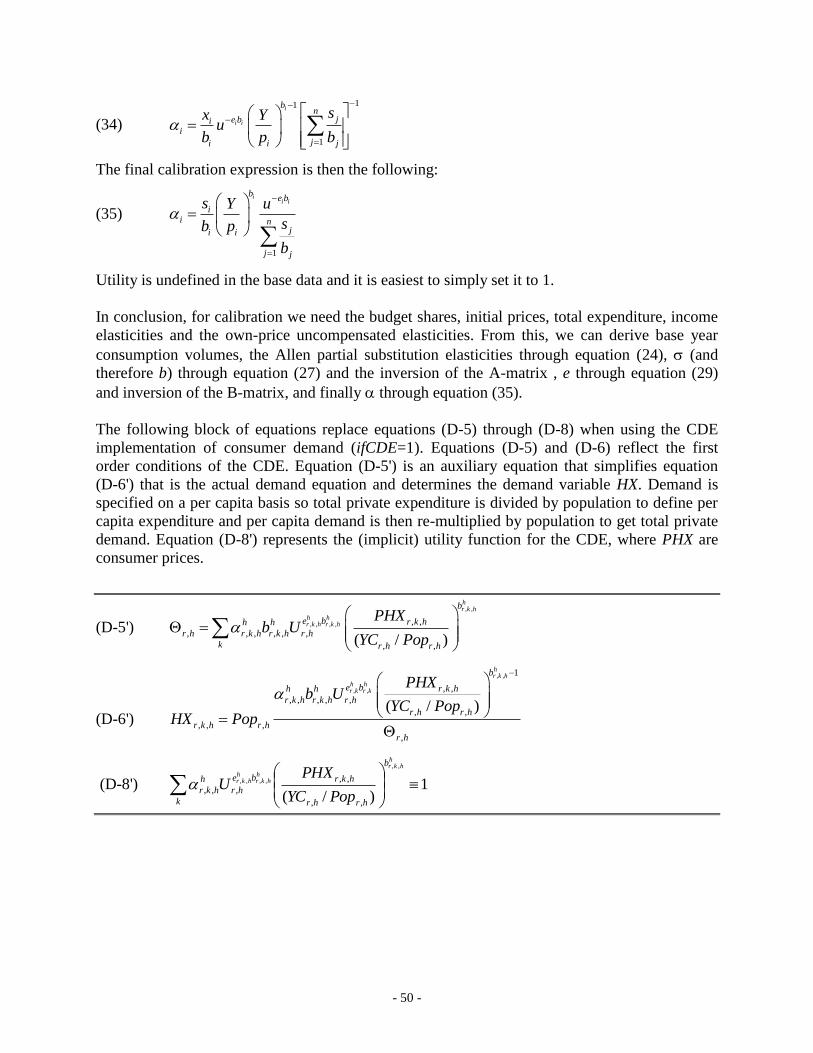
- 50 -
(34)
11
1
i
i i
bn
je bii
ji i j
sx Yu
b p b
The final calibration expression is then the following:
(35)
1
ii i
be b
ii n
ji i
j j
s Y u
sb p
b
Utility is undefined in the base data and it is easiest to simply set it to 1.
In conclusion, for calibration we need the budget shares, initial prices, total expenditure, income
elasticities and the own-price uncompensated elasticities. From this, we can derive base year
consumption volumes, the Allen partial substitution elasticities through equation (24), (and
therefore b) through equation (27) and the inversion of the A-matrix , e through equation (29)
and inversion of the B-matrix, and finally through equation (35).
The following block of equations replace equations (D-5) through (D-8) when using the CDE
implementation of consumer demand (ifCDE=1). Equations (D-5) and (D-6) reflect the first
order conditions of the CDE. Equation (D-5') is an auxiliary equation that simplifies equation
(D-6') that is the actual demand equation and determines the demand variable HX. Demand is
specified on a per capita basis so total private expenditure is divided by population to define per
capita expenditure and per capita demand is then re-multiplied by population to get total private
demand. Equation (D-8') represents the (implicit) utility function for the CDE, where PHX are
consumer prices.
(D-5')
, ,
, , , , , ,
, , , , , ,
, ,( / )
hr k h
h hr k h r k h
b
e b r k hh h
r h r k h r k h r h
k r h r h
PHXb U
YC Pop
(D-6')
, ,
, ,
1
, ,
, , , , ,
, ,
, , ,
,
( / )
hr k h
h hr k r k
b
e b r k hh h
r k h r k h r h
r h r h
r k h r h
r h
PHXb U
YC PopHX Pop
(D-8') 1)/(
,,
,,,,
,,
,,
,,,
k
b
hrhr
hkrbe
hr
h
hkr
hhkr
hhkr
hhkr
PopYC
PHXU

- 51 -
The ELES demand system
Many models assume separability in household decision making between saving and current
consumption. Lluch and Howe51
introduced a relatively straightforward extension of the LES to
include the saving decision simultaneously with the allocation of income on goods and services,
this has become known as the extended linear expenditure system or the ELES. The ELES is
based on consumers maximizing their intertemporal utility between a bundle of current
consumption and an expected future consumption bundle represented in the form of savings. The
ELES has several attractive features. The utility function of the ELES has the following form:
(36) s
i
si
iiP
Sxu
with
(37) 1 s
i
i
where u is utility, x is the vector of consumption goods, S is household saving (in value), Ps is the
price of saving, and and are ELES parameters.
The consumer solves the following problem:
(38) s
i
si
iiP
Sx
max
subject to
(39) YSxpn
i
ii 1
where p is the vector of consumer prices, and Y is disposable income. The demand functions are:
(40)
n
j
jj
i
iii pY
px
1
(41)
n
j
jj
n
j
jjs xpYpYS11
The term in parentheses is sometimes called supernumerary income, i.e. it is the income that
remains after subtracting total expenditures on the so-called subsistence (or floor) expenditures
as represented by the parameter. The parameter then represents the marginal budget share out
of supernumerary income.
From the demand equation we can derive the income and price elasticities:
51
See Lluch (1973) and Howe (1975).

- 52 -
(42) i
i
ii
ii
sxp
Y
sS
Y sss
(43)
11
i
iii
x
1s
(44) Ys
p
xp
p
i
jji
ii
jji
ij
*Y
P
sY
P jjjjs
sj
where s is the average propensity to save. Note that the matrix of elasticities can be collapsed to
a single formula using the Kronecker factor:
(45) jjij
i
iij pY
Ys
*
where takes the value 1 when i equals j and Y* is supernumerary income.
Welfare
With the addition of saving, the indirect utility function is given by:
(46) si
YP
Yp
Ypvs
s
i i
i
**),(
or
(47) P
YYpv
*
),( where
si
s
s
i i
i PpP
The expenditure function is derived by minimizing the cost of achieving a given level of utility,
u. It is set-up as:
Sxpn
i
ii 1
min
subject to
uP
Sx
s
i
si
ii
The final expression for the expenditure function is:
(48) uPpupEn
i
ii 1
,
where
(49)
si
s
s
i i
i PpP
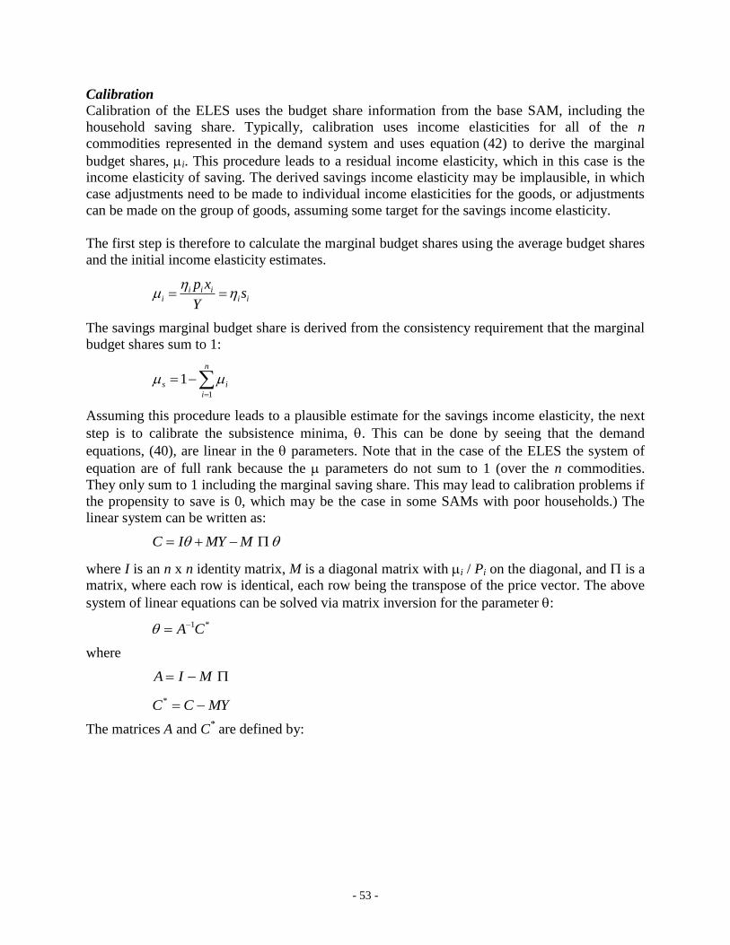
- 53 -
Calibration
Calibration of the ELES uses the budget share information from the base SAM, including the
household saving share. Typically, calibration uses income elasticities for all of the n
commodities represented in the demand system and uses equation (42) to derive the marginal
budget shares, i. This procedure leads to a residual income elasticity, which in this case is the
income elasticity of saving. The derived savings income elasticity may be implausible, in which
case adjustments need to be made to individual income elasticities for the goods, or adjustments
can be made on the group of goods, assuming some target for the savings income elasticity.
The first step is therefore to calculate the marginal budget shares using the average budget shares
and the initial income elasticity estimates.
iiiii
i sY
xp
The savings marginal budget share is derived from the consistency requirement that the marginal
budget shares sum to 1:
n
i
is
1
1
Assuming this procedure leads to a plausible estimate for the savings income elasticity, the next
step is to calibrate the subsistence minima, . This can be done by seeing that the demand
equations, (40), are linear in the parameters. Note that in the case of the ELES the system of
equation are of full rank because the parameters do not sum to 1 (over the n commodities.
They only sum to 1 including the marginal saving share. This may lead to calibration problems if
the propensity to save is 0, which may be the case in some SAMs with poor households.) The
linear system can be written as:
MMYIC
where I is an n x n identity matrix, M is a diagonal matrix with i / Pi on the diagonal, and is a
matrix, where each row is identical, each row being the transpose of the price vector. The above
system of linear equations can be solved via matrix inversion for the parameter :
*1CA
where
MIA
MYCC *
The matrices A and C* are defined by:

- 54 -
jip
p
ji
aA
i
j
i
i
ij
if
if1
i
iii
p
YxcC
*
The A and C* matrices are simplified if the price vector is initialized at 1:
ji
jiaA
i
i
ijif
if1
YxcC iii *
In GAMS one could invert the system of equations embodied in equation (40) directly by solving
for the endogenous while holding all of the other variables and parameters fixed.
The AIDADS demand system
Both the CDE and the ELES suffer from relatively poor Engel behavior. In the case of the CDE,
income elasticities stay relatively constant at their initial level irrespective of income growth.
The ELES has even worse properties as it relatively quickly converges towards a Cobb-Douglas
utility function with unitary income elasticities for all goods, even allowing for a population-
adjustment to the subsistence parameters. An alternative demand system, known as AIDADS,
has received more attention recently52
and was initially proposed by Rimmer and Powell.53
It is a
relatively natural extension to the LES function, the latter being a special case of the AIDADS
function. The insight of Rimmer and Powell was to allow the marginal propensity term of the
LES to be a function of other variables, rather than be a constant as in the LES. This allows for
more complex demand behavior, as well as providing better validation for observed changes in
consumption patterns.
Basic formulation
AIDADS starts with the implicitly additive utility function given by:
(50) i
ii uxU 1,
Assume the following functional form for the utility function:
(51)
u
iiii
Ae
xU
ln
where
52
Hertel and co-authors have been using AIDADS with the GTAP model. See for example Yu et al. (2002). 53
See Rimmer and Powell (1992a), Rimmer and Powell (1992b) and Rimmer and Powell (1996).

- 55 -
(52)
uG
uGiii
1
with the restrictions
1i
i
i
i
10 i
10 i
ii x
Cost minimization implies the following:
i
ii xpmin
subject to
(53) ln 1i ii u
i
x
Ae
The first order conditions lead to:
(54) iiiii
ii
ii
i
i pxpx
px
U
summing over i and using the fact that the i sum to unity implies:
(55) *YpYpxpi
ii
i
ii
i
ii
where Y is aggregate expenditure, and Y*, sometimes referred to as supernumerary income, is
residual expenditure after subtracting total expenditure on the so-called subsistence minima, .
Re-inserting equation (55) into (54) yields the consumer demand equations:
(56)
j
jj
i
ii
i
iii pY
pY
px
*
Equation (56) is virtually identical to the ELES demand equation (40) above. Similar to the
linear expenditure system (LES), demand is the sum of two components—a subsistence
minimum, , and a share of supernumerary income. Unlike the LES, the share parameter, , is
not constant, but depends on the level of utility itself. AIDADS collapses to the LES if each
parameter is equal to the corresponding parameter, with the ensuing function of utility, G(u),
dropping from equation (52).
Elasticities
This section develops the main expressions for the income and price elasticities. These formulas
will be needed to calibrate the initial parameters of the AIDADS function.
- 56 -
Income elasticity
To derive further properties of AIDADS requires specifying a functional form for G(u). Rimmer
and Powell (1996) propose the following:
(57) ueuG )(
The first step is to calculate the marginal budget share, , defined as:
Y
xp i
ii
The following expression can be derived from equation (56):
i
ii
ii
ii
i
i
pY
u
up
Y
Y
Y
pYp
Y
Y
x
***
Thus:
(58) Y
u
uY i
ii
*
Expression (58) can be expanded in two steps—first evaluating the partial derivative of the share
variable, , with respect to utility, and then the more difficult calculation of the partial derivative
of u with respect to income. The share formula is:
u
u
iii
e
e
1
Its derivative is:
(59)
22 )1()1(
1u
ii
u
u
uu
ii
u
i
u
i
e
e
e
eeee
u
Utility and income are combined in implicit form and thus we will invoke the implicit function
theorem to calculate the partial derivative of u with respect to Y. First, insert equation (56) into
equation (53):
i i i
u
iiu
iii
pAe
Y
Ae
x1lnln
*
Expanding the latter expression yields:
(60) 1lnlnln, *
uAY
pYuf
i i
ii
which provides the implicit relation between Y and u. The implicit function theorem states the
following:

- 57 -
(61)
1
u
f
Y
f
Y
u
The partial derivative of f with respect to Y is simply:
(62) *
1
YY
f
The partial derivative of f with respect to u is:
(63)
1
2
2
2
2
)1(
)1(ln
)1(
1ln)1(
1
ln1
u
u
iu
u
iiiiu
u
i
ii
i
i
u
u
i
ii
i
ii
i
ii
e
e
e
ex
e
e
pe
e
up
p
puu
f
where
(64)
12
1ln
iu
u
iiiie
ex
The second line uses equation (59). In the third line, equation (56) substitutes for the expression
in the logarithm, and the adding up constraint allows for the deletion of non-indexed variables.
Substituting (62) and (63) into (61) yields:
(65)
u
u
e
e
YY
u2
*
1
Substituting (59) and (65) into (58) yields:
iiii
The income elasticities are derived from the following expression:
(66) i
i
i
i
i
i
i
ii
sp
p
x
Y
Y
x
x
Y
Y
x
where si is the average budget share:
(67) Y
Y
Y
p
Y
xps i
iiiii
*
It can also be written as:

- 58 -
(68)
Y
pp
sj
jjiii
ii
Thus the income elasticity, , is equal to the ratio of the marginal budget share, , and the
average budget share, s.
Price elasticity
The matrix of substitution elasticities is identical to the expression for the ELES and has the
form:
(69) Yss
Y
ji
iijjij
*
where
ji
jiij
0
1
It is clear that the matrix is symmetric. The matrix of substitution elasticities is also equal to:
(70)
i
ii
j
ij
j
jj
i
ii
ji
iijjij
x
x
sY
Y
x
x
x
x
Yss
Y
*
*
The compensated demand elasticities derive from the following:
(72) Ys
Ys
i
iijjijjij
*
Finally, the matrix of uncompensated demand elasticities is given by:
(73) ij
i
iijjijijij s
Ys
Ys
*
The uncompensated demand elasticities can also be written as:
(73') ii
i
j
ijjj
i
iij
s
sYp
Ys
*
The first term on the right-hand side is always negative. The second term differs from the LES
expression for the uncompensated demand elasticities.54
We can see from expression (73') that
the AIDADS specification allows for both gross complementarity and substitution. As well, it
allows for luxury goods, i.e. positive own-price demand elasticities should the second term be
positive and greater than the first term.
54
Recall that for the LES, the and terms are equal and thus the second term drops.

- 59 -
Implementation
Implementation of AIDADS is somewhat more complicated than the LES since the marginal
propensity to consume out of supernumerary income is endogenous, and utility is defined
implicitly. The following four equations are needed for model implementation:
(74) i
iipYY *
(75) *Yp
xi
iii
(76) u
u
iii
e
e
1
(77) Axui
iii ln1ln
Equations (74) and (75) are identical to their LES (ELES) counterparts. Equation (76) determines
the level of the marginal propensity to consume out of supernumerary income, , which is a
constant in the case of the LES (ELES). It requires however the calculation of the utility level, u,
which is defined in equation (77).
Calibration
[To be updated] Calibration requires more information than the LES. Where the LES has 2n
parameters to calibrate (subject to consistency constraints), AIDADS has 3n parameters (less the
consistency requirements)—, and . The calibration system includes equations (74)-(77)
which have 2+2n endogenous variables (Y*, , , and A). There are no equations for calibrating
the and parameters. If we have knowledge of the income elasticities, we can add the
following equations:
(78)
iu
u
iiiie
ex
21
ln1
(79)
i
ii
i
i
i
iii
i
ii
ssss
There are an additional 1+n equations, solving for and . There is need for an additional n
equations. Assuming we have knowledge of at least n price elasticities, for example the own-
price elasticities, we can add the following equation:
(80) iiii
i
iii Yp
Ys
*
The and parameters are not independent, the following restrictions must hold:

- 60 -
(81) i
i 1
(82) i
i 1
The system is under-determined, there are 5+4n equations and 3+4n variables. One solution, is to
make the own-price elasticities endogenous. In this case, we are adding n variables, but then the
system is over-determined. We can minimize a loss function with respect to the price elasticities:
(83) i
iiL20
where 0 represents an initial guess of the own-price elasticities and the calibration algorithm will
calculate the endogenous in order to minimize the loss function, subject to constraints (78)-(82)
and the model equations (74)-(77). The exogenous parameters in the calibration procedure
include p, x, s, Y, , 0 and u.

- 61 -
Annex 3: Alternative trade specification
The GTAP database decomposes aggregate demand for goods and services by agent a into a
domestic component and an (aggregate) import component. It is this possible to implement that
Armington specification at the agent level—though the default model uses a national Armington
specification, in part to (significantly) reduce the size of the model. This short annex describes
how the model needs to be modified to allow for agent-specific behavior. Equations (T-1)
through (T-6) in the model would be replaced by the equations in the block below. Equations
(T-1') and (T-1'') define the Armington domestic and import components at the agent level,
where all share parameters and substitution elasticities are agent-specific. Equation (T-2') defines
the agent-specific Armington price. And equations (T-4') and (T-5') determine the aggregate
domestic demand for domestic production and imports respectively. Under this specification, the
variables XAT and PAT are dropped. (N.B. This specification has not been reviewed for use with
the 'energy aware' version of ENVISAGE. Among other potential issues, there are no
parameters that allow for the adding up of energy volumes in efficiency units.)
(T-1') air
ir
Ad
air
aird
airair XAPD
PAXD
mair
,,
,,,
,,
,,,,
,,
)1(
(T-1'') air
ir
Am
air
airm
airair XAPMT
PAXM
mair
,,
,,,
,,
,,,,
,,
)1(
(T-2') )1/(1
1
,,,,,
1
,,,,,,,
,,,,,,
)1()1(
mairm
airm
air
ir
Am
air
m
airir
Ad
air
d
airair PMTPDPA
(T-4') a
air
d
ir XDXDT ,,,
(T-5') a
airir XMXMT ,,,

- 62 -
Annex 4: Alternative capital account closures
[To be completed]
…has three different closures for the capital account. The simplest is simply to fix the capital
account at base year levels. The second option, as described in HT, is to allow the capital account
equilibrate changes in the expected rate of return to capital across regions, i.e. the percentage
change of regional rates of return are equal. If returns are equal initially, this is equivalent to
assuming perfect international capital mobility. The third option, also described in HT, assumes
that the ‘global’ investor has an optimal portfolio initially, and adjusts capital flows to maintain
the same portfolio ex post.
Equation (58) defines the average rate of return to capital in each region, AvgRoR. It is the
weighted average of the sectoral rates of return. [? Should the weights be fixed, i.e. indexed by t0
?]. The current net rate of return, RoRC, is then defined as the average gross regional rate of
return, adjusted by changes to the unit cost of capital, and less depreciation—equation (59).
Equation (60) defines the motion equation for aggregate capital. The end-of-period capital stock,
Kt+1, is equal to the beginning period capital stock, Kt, adjusted for depreciation, and augmented
by the current period’s volume of investment, XCInv. The expected rate of return, RoRE, is
assumed to decline with positive additions to the capital stock. This is the motivation behind
equation (61). [See HT for a more detailed description.] Equation (62) defines the value of net
investment, NInv. Equation (63) defines the average global rate of return, RoRG.
The three foreign capital closure rules are encapsulated in equation (64) and are driven by a
model flag labeled KFlowFlag. The first rule is simply to fix the capital account. To preserve
model homogeneity, the initial volume is multiplied by the model numéraire to provide a
nominal foreign saving. The second rule equates the percentage change in the expected rate of
return in each region. The third rule assumes that global investment is allocated across regions
such that the regional composition of capital stocks is invariant. This implies that the percent
change in net investment is equal across regions [Shouldn’t we be using as a rule that the capital
stock in value terms is proportionately the same across regions]. Equation (64) is defined for all
regions except for one. The left out region is indexed by RSAV that is a subset of the set of
regions, r. Closure of the model is guaranteed by equation (65) that forces the global sum of the
capital flows to be identically equal to zero.

- 63 -
Annex 5—Dynamic model equations with multi-step time periods
Dynamics in a multi-year step
The step size in the model scenarios are allowed to vary across time—in order to save compute
time and storage. Particularly in the long-run scenarios, annual increments are not particularly
useful. Some of the equations in the model—essentially almost any equation that relies on a
lagged variable need to take into account the variable step size, for example equation (G-1), the
capital accumulation equation.
1,,1,).1( Invrrrr XCKStockKStock
In fact, this equation is not even necessary in the model for a step size of 1 since both variables
on the right-hand side of the equation are lags. However, let n be the step-size, eventually 1.
Then through recursion, the capital accumulation function becomes:
n
j
jtInv
j
nt
n
t XCKStockKStock1
,
111
If the model is run in step sizes greater than 1, the intermediate values of real investment are not
calculated. They can be replaced by assuming a linear growth model for investment:
1,, 1 tInv
I
tInv XCXC
Replacing this in the accumulation function yields:
n
j
ntInv
jnIj
nt
n
t XCKStockKStock1
,
1111
With some algebraic manipulation (that is done for a number of similar expressions below), this
formula can be reduced to the following:
ntInvI
nnI
nt
n
t XCKKStock
,
111
Where we have the following equation to determine the growth rate of investment:
ntInv
nI
tInv XCXC ,, 1
which itself is now a function of contemporaneous investment. If n is equal to 1, it is clear that
this equation simplifies to the simple 1 step accumulation function. The capital accumulation
function is no longer exogenous since it depends on the investment growth rate, which itself is
endogenous. To avoid scale problems, equations (G-1a) and (G-1b) are used in place of (G-1) to
provide the n-step capital stock accumulation function. Equation (G-1a) is likely to evaluate to
somewhere between 10 and 20 since the first term is 1 plus the average annual growth of
investment, to which is added the depreciation rate less 1. If investment growth is 5% and
depreciation is also 5%, then the value is 10. The first term on the right-hand side of equation
(G-1b) is likely to be relatively small since it takes the previous capital stock and subtracts a
multiple of the previous period’s investment (lagged n years), and then multiplies by the

- 64 -
depreciation factor, so that the largest term is the second term, which is a multiple of the current
volume of investment.
(G-1a)
1/1
,,
,,
, 1
n
ntInvr
tInvr
trXC
XCIGFact
(G-1b) tInvrtr
n
trntInvrtrntrtr XCIGFactXCIGFactKStockKStock ,,,,,,,,, )1.(
The savings function, equation (D-8) also needs modification in a dynamic scenario with
multiple years between solution periods. The new equation (D-8) below shows the modification
of the savings function, where the new variables are gPLT15
and gP65UP
that represent the average
annual growth rates of the youth and elderly dependency ratios.
(D-8)
)1/(1
))1/((1
)1/(1
))1/((1
)1/(1
))1/((1)(
1
)(1
65
,
165
,65
15
,
115
,15
,
1
,,
11
,
UPP
tr
s
r
nUPP
tr
s
rUPP
r
e
r
PLT
tr
s
r
nPLT
tr
s
rPLT
tr
y
r
pc
r
s
r
npc
r
s
rpc
tr
g
r
s
ntr
ns
rs
r
ns
rs
r
s
r
s
tr
g
gDRAT
g
gDRAT
g
ggss

- 65 -
Annex 6: Climate modules
DICE 2007 Climate module
This Annex describes the climate module used in the DICE 2007 model.55
It was the climate
module used in the original version of ENVISAGE. It was replaced by the MERGE climate
module in order to handle the non-CO2 greenhouse gases. While not in current use, its
description may be of use to interested readers and the annex also shows how the DICE module
has been extended to cover any time definition—not the fixed 10-year time steps of the DICE
model.
The model contains three sinks for CO2 emissions—the atmosphere and the upper and deep
oceans. These three sinks are indexed by z. In each period, there is a flow of carbon across the
three sinks using a 3 x 3 transition matrix, . Each column of the transition matrix represents the
share of the stock in the sink that flows to a different sink. Thus the diagonal element represents
the share of the stock that stays in its own sink. The current values of the concentration transition
matrix are provided in a more detail below.
(1) , 1 , 2, 1.z z z COConc Conc EMIGbl
(2) ForcOthConcPIConc
xfCOForc atmosatmos
)2(log
)/(log.2
10
10
(3) ztztzt ForcTempTemp .. 1,
Equation (1) determines the concentration level in each sink. The concentration level is equal to
its lagged value, multiplied by the transition matrix. In the absence of new emissions, one can
determine the long-term equilibrium by multiplying the matrix n-times, where n is large
enough that the transition matrix converges towards a constant matrix. Carbon emissions are
entirely added to atmospheric concentration.56
Note that emissions in the model are in terms of
carbon. To convert to CO2, multiply the carbon emissions by the factor (44/12).
Equation (2) converts atmospheric concentrations to its impact on radiative forcing. Forcing is a
logarithmic function (based 10) of concentration with two key parameters. The first is the pre-
industrial concentration level, ConcPI. The second is the amount of forcing induced by a
doubling of concentration from its pre-industrial level, fCO2x. The relation allows for an
exogenous amount of forcing, that could eventually be negative, as is the current case, due to
SO2 emissions.
Temperature, measured as the increment to temperature in °C since 1900, like concentration, has
interactions between the atmosphere and the oceans. In this case the ocean is treated as a single
55
See Nordhaus (2008). 56
The variable EMIGbl is a vector defined overall all sinks, but emissions to the two ocean sinks are always 0.

- 66 -
sink and the subset zt of z covers only atmos and dpocn. Equation (3) provides the link between
temperature in the two sinks with their previous respective temperatures, through a transition
matrix , and the incremental impact from forcing through the matrix .57
The temperature
transition and forcing matrices are further developed below.
The transition matrices in the DICE model are based on a fixed 10-year time step between years.
In the ENVISAGE model, the time gap is variable. The model therefore requires two
modifications to the DICE version of the climate module. First, it is necessary to convert the 10-
year transition matrices to a single-year transition matrix, and then to code the dynamic
equations to allow for variable gap dynamic expression.
Emissions and concentration
In the DICE model, the 10-year concentration transition matrix has the following form and
values:
0.9968810.0500000
0.0031190.8527870.189288
00.0972130.810712
333231
232221
131211
dpocn
upocn
atmos
dpocnupocnatmos
bbbdpocn
bbbupocn
bbbatmos
dpocnupocnatmos
Nearly 19% of atmospheric carbon is absorbed by the upper sea (over a decade), and the upper
sea releases about 10% of its carbon to the atmosphere (over a decade).
If emissions end at some point T, then the equilibrium concentration of carbon can be given by
the following equation:
TConcConc
The equilibrium matrix, ∞, is given by:
0.9137390.9137390.913739
0.0569910.0569910.056991
0.0292690.0292690.029269
dpocn
upocn
atmos
dpocnupocnatmos
This implies that in the long run the atmosphere will contain just under 3% of total carbon in all
three physical zones (or sinks) as of the terminal year of emissions, with about 6% in the upper
ocean and the remaining 91% absorbed in the deep ocean. At today’s level of carbon
concentrations we would get the following equilibrium concentration levels (assuming all
emissions stop today):58
57
The variable Forc is a vector defined over both sinks but is only non-zero for the atmosphere. 58
The concentration is expressed at the stock of carbon (C) in gigatons.

- 67 -
365,18
255,1
809
667,18
164,1
598
Conc
This translates into a reduction of 26 percent in atmospheric concentration and a rise of 1.6% in
deep ocean concentration. If the entire estimated amount of fossil fuels is spewed out into the
atmosphere, over the very long run, the atmospheric concentration would stabilize at 713 GTC,
lower than today’s level, but in the intermediate years, concentration levels could rise
dramatically. In the DICE baseline with no mitigation efforts, concentration levels in the
atmosphere max out at around 3,000 GTC in around 2250.
The matrix is valid for a time horizon spanning 10 years. In other words, equation (C-14) in
terms of the DICE model is:
ttztz ECConc ,10,
where Et represents the cumulated emissions over 10 years through year t. It is possible to
convert into an annual transition matrix with some matrix algebra and numerical evaluation. If
the matrix is a positive definite matrix, than all of its eigenvalues are positive and it is possible
to take the nth
root of the matrix . The eigenvalues and eigenvectors of a real matrix solve the
following matrix equation:
xx
In other words the projection of the vector x, by the matrix is equal to that same vector
multiplied by a scalar, . The eigenvalues, , can be calculated by solving an n-degree
polynomial derived from the determinant of the above system:
0.0. IxIxx
Let V be the matrix of (right) eigenvectors of (in columns), and the diagonal matrix
composed of the eigenvalues (in the same order as the respective eigenvectors), then is
diagonalized by:
1 VV
It can be shown that if has only positive eigenvalues59
, than the nth
root of can be derived
from60
:
59
If the diagonal elements of a square matrix B are all positive, and if B and B' are both diagonally dominant, then
B is positive definite. The definition of diagonally dominant is that the absolute value of each diagonal element
is greater than the sum of absolute values of the non-diagonal elements in its row. That is if for all i |a(i,i)| >
Sum(|a(i,j)|;j != i). 60
It is pretty easy to see this if n=2:

- 68 -
1/1/1 VV nn
In the case of the matrix above, a numerical package has been used to numerically calculate
the eigenvalues and eigenvectors61
:
1.00000000
00.9661220
000.694258
0.9975510.8093690.125829-
0.0622190.497912-0.761574
0.0319540.311457-0.635745-
V
Thus the annual transition matrix is given by:
0.9996800.0054130.000545-
0.0003380.9830210.022520
0.000017-0.0115660.978025110/110/1 VV
Intuitively, one can see that the diagonal elements of are roughly equal to the diagonal
elements of raised to the power 0.1 and that the off-diagonal elements are roughly 10% of the
off-diagonal elements of .
[N.B. The third eigenvector reflects the same distribution as the long-run equilibrium distribution
described in note 1 above, corresponding to the eigenvalue 1. The equilibrium matrix can also be
derived from the following formula:
0.9137390.9137390.913739
0.0569910.0569910.056991
0.0292690.0292690.029269
100
000
00011 VVVVLim n
n
]
Equation (C-4) can then be written in cumulative form as:
1
0
1n
j
njt
jn
nt
n
t EConcConc
Assuming that emissions grow at a compound growth rate of ge between t-n and t, we have the
following:
BVVVVVVBCCBVVC 12/12/112/112/12/112/1 ...
In the next to the last step the square root of the diagonal matrix is simply the square root of each diagonal
element and the multiplication of the two diagonal matrices is simply the original diagonal matrix. This is easy
to generalize for any integer root. 61
The eigenvectors are determined up to a scalar multiple. In the case above, they have been normalized to be on
the unit circle.

- 69 -
nt
n
j
jnjnn
nt
n
n
j
nt
jnjnn
nt
n
n
j
jt
jjn
nt
n
t
EVgVgConc
EVgVgConc
EgConcConc
11
0
111
1
0
1111
1
0
1
1
)1()1(
)1()1(
)1(
The expression within brackets is a diagonal matrix, so it is possible to use standard formulas for
a geometric progression to give the following:
ntnt
n
t EVVConcVVConc
11
where is defined as above, and the diagonal matrix is given by:
ji
jig
ge
i
nen
i
ij
if0
if)1(
)1(
Based on these expressions, equation (1) that defines concentration for a one period gap is
replaced by equations (4), (5) and (6). Equation (4) determines the growth of emissions between
period t-n and t assuming a constant annual growth rate, gemi
. Equation (5), similar to the
expression above, defines a 3 x 3 matrix, EMIGFact, which is used to determine the growth
factor in the cumulative concentration expression. The parameter c in the expression represents
the eigenvalues of the transition matrix . And equation (6), replacing equation (1) determines
the cumulative concentration, Conc, in period t. The first component on the right is the evolution
of the existing stock of carbon concentration where Vc is the matrix of eigenvectors of the
matrix and c is the diagonal matrix of eigenvalues. The second component represents
cumulative emissions over the period n, with adjustments for the transition of the lagged
emissions across the sinks.
(4) 1
/1
,,
,,
,
n
ntemArmos
temArmosemi
temEMIGbl
EMIGblg
(5) )1(
)1()(
,
,
, emi
tem
c
z
nemi
tem
nc
z
tzg
gEMIGFact
(6) ntCOz
c
t
c
nt
cncc
t EMIGblVEMIGFactVConcVVConc
,2,
11).44/12()(

- 70 -
Temperature
The temperature transition, similar to concentration, has to be modified to allow for multiple year
gaps. This section describes how the DICE formulation has been adapted for variable time steps.
The temperature module in DICE can be collapsed into matrix form:
FTFTMT .0
.1
)(1..
1
1
33
2121
1
where the transition and impact matrices, M and B are defined for a 10-year transition period. In
the steady-state, this can be written as:
FBMIT e .1
where F is a constant level of radiative forcing. The inverse matrix has a rather simple
expression:
)/()()/(1
)/()/(1
321
1211
MI
This implies that the equilibrium temperature for both the atmosphere and the deep ocean is
given simply by:
/FT e
With the default value for , the equilibrium temperature is about 0.8 times the equilibrium
forcing level.
Similar to the concentration equation above, the temperature equation is recursive and can be
collapsed into multi-period form by the following formula:
ntt
n
nt FVVTVVT
.11
Where is the diagonal matrix of eigenvalues of the one-period transition matrix, and the
diagonal matrix is given by:
ji
jigg
gnfnf
i
nfn
i
ij
if0
if)1()1(
)1(1
where gf is the annual compound growth rate of forcing (F) over the n-period range.

- 71 -
There are two differences with the concentration accumulation equation. The first is that the
forcing variable, F, is pre-multiplied by the matrix . The second is that in the DICE code the
forcing variable is contemporaneous and not lagged—this changes the accumulation expression
compared to the one for concentration. Both nevertheless collapse to 1 when n is equal to 1.
Similar to the concentration matrix, but with additional complications, one must convert the
DICE-based 10-period M and B matrices into a 1-period matrix—hopefully preserving as well
the particular relations across the different cells of the matrices. The following steps provide one
way to do this:
1. Calculate the 10-period eigenvalues and eigenvectors of the 10-period M matrix so that the
following holds:
1 VVM
2. Calculate the 1/10th
roots of the eigenvalues and then evaluate the 1-period M matrix, :
11.0 VV
3. Calculate the coefficients consistent with the values of the cells in . There are too few
degrees of freedom, so some choices must be made. For example:
1211
122
1
2
121
213 322 1
Thus, the bottom right cell of is adjusted so that the sum along the bottom row is 1. The one-
period matrix, 1 then becomes:
11
4. Since the matrix has been modified, it is necessary to re-calculate the eigenvalues and
eigenvectors consistent with the adjusted 1-period matrix. The new one-period coefficients
and the one-period eigenvalues and eigenvectors can be used for models that use one- or multi-
period steps.
Equations (2) and (3) are then replaced with (7) and (8), (9) and (10). In equation (7) the only
difference with Equation (2) is that the expression uses the average concentration between years
t-n and t, rather than the concentration of a single year. Equation (8) defines the average annual
growth rate in forcing, gf, between years t-n and t. Equation (9) defines a 2 x 2 diagonal matrix
that is used to provide the forcing growth factor, ForcGFact, for the cumulative temperature
transition equation. It is similar to expression (5) save that the denominator is adjusted to account
for the fact that forcing is assumed to impact current temperatures, and not future temperatures,
i.e. forcing and temperature are contemporaneous variables. The t parameters are the
eigenvalues of the temperature transition matrix. Equation (10) represents the
temperature/forcing relation for a multi-year transition period, where Vt is the matrix of

- 72 -
eigenvectors of the temperature transition matrix, t is the matrix of eigenvalues, and is the
direct impact of forcing on temperature.
(7)
ForcOthConcPIConcConc
xfCOForctatmosntatmos
atmos
)2(log
/)(5.0log.2
10
,,10
(8) 1
n
nt
tf
tForc
Forcg
(9) )1()1(
)1()(1, f
t
nf
t
t
zt
nf
t
nt
zttzt
gg
gForcGFact
(10) zt
t
t
t
ntzt
tntt
tzt ForcVForcGFactVTempVVTemp .)(1
,
1
,

- 73 -
Annex 7: Examples of carbon taxes, emission caps and tradable permits
Border tariff adjustment simulations
Border tariff adjustments (BTAs) have been a hotly contested subject since at least the early
negotiations over the Kyoto Protocol. The issue arises when a small coalition of countries
unilaterally implement emission reduction policies that raise domestic energy prices but have no
direct impact on energy prices outside the coalition. This has two consequences. The first is that
the coalition countries witness a loss in competitiveness and therefore market share—both at
home and on export markets. And, their emission reduction efforts could be partially—or even
entirely—offset by rising emission in non-coalition countries, the so-called carbon leakage effect.
One response to either or both of these effects is to raise a carbon tax on competing imports
thereby raising the relative price of imports with the aim of neutralizing the competiveness effect
without of course affecting directly market shares in other countries. The coalition countries are
also likely to rebate the carbon tax to exporters to maintain competitiveness outside the coalition.
If the main concern is competitiveness, coalition countries could use the domestic carbon content
to calculate the needed border tax adjustment. On the other hand, if the main concern is leakage,
there could be a case for using the carbon content of the import competing countries under an
assumption that all producers would therefore be paying the same price for their carbon
emissions. This section describes how the ENVISAGE model has been modified to handle BTAs
under these different assumptions.
Adjustment based on carbon content of domestic producers (or importers)
The main idea is to level the playing field for domestic producers. The model calculates how
much the costs of production increase due to both the direct and indirect effects of the carbon tax.
It is an ex ante calculation in the sense that the cost structure of a reference year is chosen before
implementation of the BTA and assumes a given price and production structure. In a GE
framework prices and quantities will adjust so that the ex post increase in cost is likely to be
lower than the ex ante increase thus the BTA will over-compensate domestic producers.
Equation (A7-1) defines the ex ante increase in unit cost, PX1, generated by the carbon tax,
where the year tr, refers to a reference year prior to the implementation of the BTA and the
super-scripted price variables are the prices that reflect the direct and indirect costs of the carbon
tax. It assumes therefore a fixed technology and the same prices for factors—but augments the
cost of intermediate goods by the carbon tax. The new unit cost will include both the direct and
indirect costs of the carbon tax. Equation (A7-2) determines the ex ante price of intermediate
goods, PA1. It is assumed that the increase in intermediate goods is equal to the increase in the
unit cost. Equations (A7-1) and (A7-2) represent a recursive system in prices that will generate in
the end the relative increase in the unit cost of production induced by carbon taxation. Equation
(A7-3) calculates the ex-ante wedge in the unit cost, d, i.e. the wedge that is induced by the
carbon tax given the cost structure of the reference year. Equation (A7-4) calculates the
equivalent tariff that is applied to imported goods that offsets the ex ante increase in the cost of
domestic production. A complicating factor is the multi-output structure of production. This is

- 74 -
dealt with by taking the weighted average of the different production streams (indexed by a) to
produce commodity, i. The weights are represented by the p parameter and are calculated using
the reference year shares:
, ,
, ,
, , , ,
0
,
, , , ,
0
pr a i
pr a i
r a tr r a tr
ap
r a
r i tr r i tr
a
PP XP
PS XS
For most commodity/activity combinations there is a one-to-one correspondence and the p
parameter takes the value 1. Note that equations (A7-1) and (A7-2) hold for all activities and
commodities, whereas equation (A7-4) is only applied to a subset of commodities indexed by it.
The index r represents countries that are self-imposing a carbon tax, whereas the index r' in
equation (A7-4) is for all countries that are not limiting emissions. Thus, even if there is uneven
effort (or uneven carbon taxes) across countries with GHG emission limits, there is no
assumption that a compensating mechanism will be in effect among these countries.
(A7-1)
1
, , , , , , , , , , , , , , , , , , , ,
1
, ,
, ,
emi
r i a t r i a tr r fp a tr r fp a tr r em t r em i a r i a tr
i fp i em
r a t
r a tr
PA XA PF XF XA
PXXP
(A7-2) , ,
, ,
1
, ' , ',
' 01
, , , , ,
, ' , ',
' 0
pr a i
pr a i
p
r a r a t
a
r i a t r i tr p
r a r a tr
a
PX
PA PAPX
(A7-3)
1
, , , ,
, ,
, ,
r a t r a trd
r a t
r a tr
PX PX
PX
(A7-4)
, ,
', , , , , ,
0pr a it
a p d
r r it t r a r a t
a
Most border adjustment regimes would also include a cost-compensation for exports. A
symmetric additive adjustment factor can be included to existing export taxes subsidies.
Equation (A7-5) defines the export subsidy adjustment, where r is the exporting country and has
imposed a carbon tax, and r' is a destination country with no carbon tax.
(A7-5)
, ,
, ', , , , ,
0pr a it
ae p d
r r it t r a r a t
a
These new instruments require changes to equations that contain bilateral tariffs and/or export
tax subsidies. This reduces to four equations—equations (T-7) and (T-9) that define bilateral

- 75 -
trade prices, FOB and end-user respectively; and equations (Y-3) and (Y-4) that determine fiscal
revenues associated with import tariffs and export subsidies respectively.
(T-7') imrr
e
imrrimrr PEWPE ,',,',,', )1(
(T-9') imrr
m
imrrimrr WPMPM ,',,',,', )1(
(Y-3') , ', , ', , ', , ', , , ,
'
m a d m
r ttax r r i r r i r r i r r i r i i r i
i Arm r i Arm
GREV WPM WTF PW XMT
(Y-4') , , ', , ', , ', , ', , ,
'
e ae s e
r etax r r i r r i r r i r r i r i i r i
i Arm r i Arm
GREV PE WTF PW XET
Adjustment based on carbon content of exporters
A tax on the carbon content of imports may help to attenuate the leakage effect of unilateral
carbon taxes. The implementation involves assessing the ex ante cost of production in the
exporting countries (i.e. those not imposing a carbon tax) applying the carbon tax of the
destination country. This implies that the cost wedge and the tariff adjustment will vary across
exporting countries for the same destination economy, unlike the adjustment above where the
tariff adjustment is uniform across importing countries.
Equation (A7-6) defines the fictitious carbon tax that is imposed on the cost of production in the
exporting country. It is bilateral as each of the importing countries has a different carbon tax.
Equation (A7-7) defines the ex ante increase in unit cost, PX2, generated by the carbon tax,
where the year tr, refers to a reference year prior to the implementation of the BTA and the
super-scripted price variables are the prices that reflect the direct and indirect costs of the carbon
tax. It assumes therefore a fixed technology and the same prices for factors—but augments the
cost of intermediate goods by the carbon tax. The new unit cost will include both the direct and
indirect costs of the carbon tax. It is a bilateral price as the carbon tax differs across countries of
destination. Equation (A7-8) determines the ex ante price of intermediate goods, PA2. It is
assumed that the increase in intermediate goods is equal to the increase in the unit cost. Equation
(A7-9) calculates the ex-ante wedge in the unit cost, m, i.e. the wedge that is induced by the
carbon tax given the cost structure of the reference year. Equation (A7-10) calculates the
equivalent tariff that is applied to imported goods that offsets the ex ante increase in the cost of
domestic production. Note that equations (A7-7) through (A7-9) hold for all activities and
commodities, whereas equation (A7-10) is only applied to a subset of commodities indexed by it.
The index r' represents countries that are self-imposing a carbon tax, whereas the index r is for
all countries that are not limiting emissions.
- 76 -
(A7-6) ,2
', , , ', ,
emi emi
r r em t r em t
(A7-7)
2 ,2
', , , , , , , , , , , , , ', , , , , , , , ,
2
', , ,
, ,
emi
r r i a t r i a tr r fp a tr r fp a tr r r em t r em i a r i a tr
i fp i em
r r a t
r a tr
PA XA PF XF XA
PXXP
(A7-8) , ,
, ,
2
, ' ', , ',
' 02
', , , , , ,
, ' , ',
' 0
pr a i
pr a i
p
r a r r a t
a
r r i a t r i tr p
r a r a tr
a
PX
PA PAPX
(A7-9)
2
', , , , ,
', , ,
, ,
r r a t r a trm
r r a t
r a tr
PX PX
PX
(A7-10)
, ,
, ', , , ', , ,
0pr a it
a p d
r r it t r a r r a t
a
Some scenarios allow for compensating a subset of regions for the imposition of a carbon tax.
Thus while high-income countries benefit from a uniform global price on carbon, developing
countries may not desire to impose a tax that could be harmful to their economy, especially since
high-income countries are as at present mostly responsible for the current stock of GHG
atmospheric concentration. The compensation mechanism is implemented as a government to
government transfer, GTR. Given the fiscal closure rule, this implies that direct taxes on
households will shift—lower taxes for receiving countries and higher taxes for donor countries.
Equation (A7-11) guarantees that the sum of the transfers adds up to zero globally where
countries are divided into donor and recipient countries. (N.B. The transfers are not bilateral.)
Equation (A7-12) is an allocation mechanism across donor countries that insures that the
transfers are equalized on a per capita basis.
(A7-11) 0r r
r Donors r Recipients
GTR GTR
(A7-12) / forr rGTRpc GTR Pop r Donors
The implementation requires exogenizing some objective for the recipient countries. In the
standard implementation, real domestic absorption is fixed to baseline values, where the
superscript BaU refers to the baseline level:
, , forBaU
r t r tRYD RYD r Recipients
The addition of the new GTR variable requires a change to the government revenue equation:
(Y-8') ,
E
r r gy em r
gy em
YG GREV QuotaY GTR

- 77 -
Annex 8: Base ENVISAGE parameters
Like most CGE models, ENVISAGE contains a mix of calibrated and key parameters—the latter
sourced from a variety of studies. The basic framework of a comparative static CGE model is
that a base year data set is given—the GTAP world social accounting matrix (SAM), for example.
This represents value flows. Base prices are typically initialized at unit value, with some
exceptions if volume flows and/or stocks are available—for example energy in physical units or
the stock of labor. Parameters are then divided into two sets: key parameters—typically
substitution, supply, price and income elasticities, and calibrated parameters. The model can be
represented compactly by the following formula:
1 2( , ; , ) 0F Y X
where Y represents endogenous variables, X is the set of exogenous variables including policy
instruments, 1 is the set of key parameters and 2 is the set of calibrated parameters. The key
parameters are given and typically estimated using outside sources and data. In the calibration
phase, both Y and X are given (by the base year data), and the function F is inverted to calibrate
the 2 parameters such that the model can replicate the base year data.62
Alternative scenarios
then involve perturbing one or more elements in X and inverting the function F to calculate a
new Y, the set of endogenous variables, holding 1 and 2 constant. Note that sensitivity analysis
on 1, the key parameters, typically requires re-calibrating 2 for each new set of 1. The rest of
this annex presents the key parameter values used for ENVISAGE.
Production elasticities
The basic production substitution elasticities are provided in Tables A8.1 and A8.2. They
replicate those used for the OECD GREEN model (see Burniaux et al 1992) and likewise
underlie the World Bank’s LINKAGE model. The original OECD GREEN model had a single
energy nest rather than the nested structure of ENVISAGE. The uniformity of the energy
substitution elasticities therefore replicates the structure of GREEN.
Table A8.1 Production parameters
Name Symbol Old New Note sigmap
p 0.00 0.00
sigmav v 0.12 1.00 Leontief technology in fossil fuel production
sigmake ke
0.00 0.80 Leontief technology in fossil fuel production sigman
n 0.00 0.00 Not differentiated by vintage
62
Invariably, calibration can be done block by block and does not involve actually inverting F as a complete
system of equations.

- 78 -
Table A8.2 Energy substitution elasticities in production
Name Symbol Old New Note sigmae
e 0.25 2.00
sigmanely nely
0.25 2.00 sigmaolg
olg 0.25 2.00
sigmaely ely
0.25 2.00 sigmacoa
coa 0.25 2.00
sigmaoil oil
0.25 2.00 sigmagas
gas 0.25 2.00
Final demand elasticities
Consumer final demand elasticities in the ENVISAGE models are derived in large part from
estimates produced by the Economic Research Service (ERS) of the U.S. Department of
Agriculture (USDA).63
The available estimates are for a reduced set of goods and these estimates
are allocated over the 57 sectoring scheme of GTAP. They are aggregated using GTAP
consumption shares for specific aggregations of GTAP. Table A8.3 provides the income
elasticities for all 57 GTAP goods for a selected aggregation across GTAP regions.64
The
calibration procedure of ENVISAGE may make some adjustments to these elasticities to insure
that the consumption weighted sum of the income elasticities adds up to unity. Table A8.4
provides the initial price elasticities used in the calibration procedure for the same aggregate
regions as in Table A8.3—again using simple averages within regions rather than consumption
weighted.
Equations (D-12) through (D-13) convert consumed goods to produced goods using a transition
matrix approach with a CES preference structure. The transition matrix is currently diagonal
63
Regmi 2001, Seale et al 2003 and Regmi and Seale 2010. 64
Regional aggregations in Table A8.3 are simple—not consumption weighted.

- 79 -
Table A8.3 Consumer income elasticities for select regions CHN XEA IND XSA RUS XEC MNA SSA LAC WEU JPN USA RHY
PDR 0.19 0.46 0.49 0.49 0.40 0.41 0.43 0.52 0.38 0.22 0.16 0.05 0.18
WHT 0.19 0.46 0.48 0.49 0.40 0.40 0.42 0.52 0.38 0.22 0.16 0.05 0.18
GRO 0.19 0.46 0.49 0.49 0.40 0.40 0.42 0.43 0.38 0.22 0.16 0.05 0.18
V_F 0.38 0.55 0.58 0.55 0.50 0.49 0.51 0.50 0.48 0.33 0.24 0.08 0.29
OSD 0.23 0.48 0.50 0.52 0.43 0.43 0.45 0.54 0.41 0.25 0.18 0.06 0.21
C_B 0.48 0.74 0.76 0.77 0.65 0.66 0.68 0.76 0.64 0.43 0.31 0.11 0.39
PFB 0.91 0.92 0.92 0.92 0.91 0.91 0.91 0.92 0.91 0.91 0.90 0.90 0.91
OCR 0.48 0.73 0.74 0.75 0.65 0.66 0.68 0.68 0.63 0.43 0.31 0.11 0.38
CTL 0.48 0.74 0.77 0.74 0.66 0.65 0.68 0.74 0.64 0.43 0.31 0.11 0.39
OAP 0.48 0.70 0.75 0.74 0.65 0.65 0.68 0.74 0.64 0.43 0.31 0.11 0.39
RMK 0.51 0.81 0.84 0.76 0.68 0.71 0.74 0.84 0.69 0.46 0.33 0.12 0.41
WOL 0.91 0.92 0.92 0.92 0.91 0.91 0.92 0.92 0.91 0.91 0.90 0.90 0.91
FRS 1.26 1.47 1.49 1.47 1.33 1.37 1.36 1.70 1.34 1.26 1.24 1.22 1.25
FSH 0.53 0.79 0.87 0.84 0.74 0.75 0.77 0.87 0.72 0.48 0.34 0.12 0.42
COA 1.17 1.23 1.24 1.24 1.19 1.21 1.20 1.27 1.20 1.17 1.16 1.15 1.16
OIL 1.18 1.25 1.26 1.26 1.21 1.22 1.22 1.29 1.21 1.18 1.17 1.16 1.17
GAS 1.17 1.23 1.24 1.24 1.19 1.20 1.20 1.27 1.20 1.17 1.16 1.15 1.16
OMN 1.26 1.48 1.50 1.49 1.33 1.37 1.36 1.74 1.35 1.26 1.24 1.22 1.25
CMT 0.48 0.73 0.77 0.77 0.61 0.65 0.67 0.74 0.60 0.42 0.31 0.10 0.38
OMT 0.48 0.70 0.77 0.77 0.64 0.65 0.64 0.72 0.61 0.41 0.31 0.10 0.38
VOL 0.24 0.46 0.51 0.48 0.42 0.43 0.45 0.51 0.39 0.25 0.18 0.06 0.20
MIL 0.51 0.79 0.82 0.82 0.69 0.69 0.71 0.83 0.66 0.43 0.33 0.11 0.41
PCR 0.19 0.39 0.46 0.38 0.40 0.41 0.43 0.49 0.36 0.22 0.15 0.05 0.17
SGR 0.48 0.73 0.76 0.73 0.64 0.66 0.67 0.74 0.63 0.43 0.31 0.11 0.38
OFD 0.48 0.61 0.72 0.73 0.61 0.62 0.64 0.58 0.57 0.39 0.27 0.08 0.36
B_T 0.58 0.90 1.07 1.03 0.85 0.87 0.90 1.18 0.79 0.51 0.36 0.12 0.45
TEX 0.91 0.87 0.88 0.86 0.91 0.90 0.89 0.88 0.89 0.89 0.90 0.90 0.90
WAP 0.91 0.84 0.92 0.90 0.89 0.90 0.87 0.88 0.86 0.88 0.89 0.88 0.88
LEA 0.91 0.89 0.92 0.92 0.91 0.91 0.91 0.91 0.89 0.90 0.90 0.90 0.90
LUM 1.26 1.47 1.50 1.49 1.32 1.36 1.35 1.73 1.33 1.26 1.24 1.22 1.25
PPP 1.26 1.46 1.49 1.49 1.33 1.36 1.35 1.73 1.32 1.24 1.23 1.21 1.24
P_C 1.18 1.15 1.20 1.24 1.17 1.19 1.17 1.25 1.14 1.14 1.15 1.14 1.15
CRP 1.27 1.41 1.48 1.45 1.30 1.34 1.33 1.67 1.26 1.23 1.23 1.20 1.23
NMM 1.26 1.47 1.50 1.48 1.33 1.37 1.35 1.73 1.34 1.26 1.24 1.22 1.25
I_S 1.26 1.48 1.50 1.49 1.33 1.37 1.36 1.74 1.34 1.26 1.24 1.22 1.25
NFM 1.26 1.47 1.50 1.49 1.33 1.37 1.36 1.74 1.34 1.26 1.24 1.22 1.25
FMP 1.26 1.47 1.49 1.49 1.33 1.37 1.36 1.73 1.34 1.26 1.24 1.22 1.25
MVH 1.18 1.17 1.26 1.25 1.18 1.20 1.18 1.27 1.18 1.13 1.15 1.13 1.14
OTN 1.18 1.23 1.26 1.26 1.21 1.22 1.21 1.29 1.19 1.17 1.17 1.15 1.17
ELE 1.27 1.41 1.49 1.48 1.33 1.36 1.35 1.73 1.31 1.25 1.22 1.21 1.22
OME 1.27 1.43 1.49 1.49 1.31 1.34 1.35 1.73 1.32 1.24 1.23 1.20 1.23
OMF 1.26 1.41 1.49 1.48 1.32 1.36 1.34 1.71 1.30 1.24 1.23 1.21 1.23
ELY 1.17 1.17 1.22 1.21 1.12 1.13 1.16 1.24 1.16 1.13 1.15 1.14 1.15
GDT 1.17 1.23 1.24 1.24 1.18 1.17 1.20 1.27 1.20 1.17 1.16 1.15 1.16
WTR 1.17 1.23 1.24 1.24 1.18 1.20 1.20 1.25 1.19 1.16 1.15 1.14 1.16
CNS 1.17 1.23 1.24 1.24 1.19 1.20 1.20 1.26 1.19 1.16 1.16 1.15 1.16
TRD 1.19 0.92 1.17 1.19 0.97 1.11 1.08 1.08 1.03 1.01 0.99 0.98 0.94
OTP 1.18 1.19 1.22 1.15 1.15 1.18 1.18 1.23 1.12 1.14 1.13 1.14 1.14
WTP 1.18 1.25 1.25 1.23 1.20 1.22 1.22 1.29 1.21 1.17 1.17 1.16 1.17
ATP 1.18 1.22 1.26 1.23 1.20 1.21 1.21 1.28 1.19 1.17 1.16 1.16 1.15
CMN 1.18 1.22 1.26 1.25 1.20 1.20 1.20 1.27 1.17 1.15 1.15 1.13 1.15
OFI 1.27 1.44 1.49 1.49 1.33 1.36 1.34 1.70 1.30 1.23 1.23 1.15 1.22
ISR 1.26 1.45 1.50 1.48 1.33 1.37 1.35 1.72 1.32 1.24 1.21 1.18 1.22
OBS 1.27 1.41 1.48 1.46 1.28 1.33 1.27 1.67 1.31 1.09 1.22 1.21 1.22
ROS 1.33 1.71 1.79 1.71 1.42 1.52 1.47 2.47 1.41 1.28 1.23 1.16 1.25
OSG 1.28 1.42 1.49 1.46 1.30 1.36 1.29 1.77 1.25 1.19 1.18 0.99 1.16
DWE 1.18 1.06 1.18 1.18 1.20 1.19 1.17 1.21 1.02 1.16 1.02 0.99 1.03 Note: The regional abbreviations are China (CHN), Rest of East Asia & Pacific (XEA), India (IND), Rest of South Asia (XSA), Russia
(RUS), Rest of Europe & Central Asia (XEC), Middle East & North Africa (MNA), Sub-Saharan Africa (SSA), Latin America & Caribbean
(LAC), Western Europe (WEU), Japan (JPN), the United States (USA), and Rest of High-income (RHY).
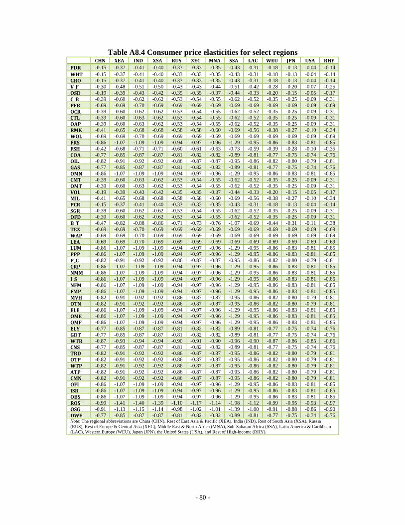
- 80 -
Table A8.4 Consumer price elasticities for select regions CHN XEA IND XSA RUS XEC MNA SSA LAC WEU JPN USA RHY
PDR -0.15 -0.37 -0.41 -0.40 -0.33 -0.33 -0.35 -0.43 -0.31 -0.18 -0.13 -0.04 -0.14
WHT -0.15 -0.37 -0.41 -0.40 -0.33 -0.33 -0.35 -0.43 -0.31 -0.18 -0.13 -0.04 -0.14
GRO -0.15 -0.37 -0.41 -0.40 -0.33 -0.33 -0.35 -0.43 -0.31 -0.18 -0.13 -0.04 -0.14
V_F -0.30 -0.48 -0.51 -0.50 -0.43 -0.43 -0.44 -0.51 -0.42 -0.28 -0.20 -0.07 -0.25
OSD -0.19 -0.39 -0.43 -0.42 -0.35 -0.35 -0.37 -0.44 -0.33 -0.20 -0.15 -0.05 -0.17
C_B -0.39 -0.60 -0.62 -0.62 -0.53 -0.54 -0.55 -0.62 -0.52 -0.35 -0.25 -0.09 -0.31
PFB -0.69 -0.69 -0.70 -0.69 -0.69 -0.69 -0.69 -0.69 -0.69 -0.69 -0.69 -0.69 -0.69
OCR -0.39 -0.60 -0.62 -0.62 -0.53 -0.54 -0.55 -0.62 -0.52 -0.35 -0.25 -0.09 -0.31
CTL -0.39 -0.60 -0.63 -0.62 -0.53 -0.54 -0.55 -0.62 -0.52 -0.35 -0.25 -0.09 -0.31
OAP -0.39 -0.60 -0.63 -0.62 -0.53 -0.54 -0.55 -0.62 -0.52 -0.35 -0.25 -0.09 -0.31
RMK -0.41 -0.65 -0.68 -0.68 -0.58 -0.58 -0.60 -0.69 -0.56 -0.38 -0.27 -0.10 -0.34
WOL -0.69 -0.69 -0.70 -0.69 -0.69 -0.69 -0.69 -0.69 -0.69 -0.69 -0.69 -0.69 -0.69
FRS -0.86 -1.07 -1.09 -1.09 -0.94 -0.97 -0.96 -1.29 -0.95 -0.86 -0.83 -0.81 -0.85
FSH -0.42 -0.68 -0.71 -0.71 -0.60 -0.61 -0.63 -0.73 -0.59 -0.39 -0.28 -0.10 -0.35
COA -0.77 -0.85 -0.87 -0.87 -0.81 -0.82 -0.82 -0.89 -0.81 -0.77 -0.75 -0.74 -0.76
OIL -0.82 -0.91 -0.92 -0.92 -0.86 -0.87 -0.87 -0.95 -0.86 -0.82 -0.80 -0.79 -0.81
GAS -0.77 -0.85 -0.87 -0.87 -0.81 -0.82 -0.82 -0.89 -0.81 -0.77 -0.75 -0.74 -0.76
OMN -0.86 -1.07 -1.09 -1.09 -0.94 -0.97 -0.96 -1.29 -0.95 -0.86 -0.83 -0.81 -0.85
CMT -0.39 -0.60 -0.63 -0.62 -0.53 -0.54 -0.55 -0.62 -0.52 -0.35 -0.25 -0.09 -0.31
OMT -0.39 -0.60 -0.63 -0.62 -0.53 -0.54 -0.55 -0.62 -0.52 -0.35 -0.25 -0.09 -0.31
VOL -0.19 -0.39 -0.43 -0.42 -0.35 -0.35 -0.37 -0.44 -0.33 -0.20 -0.15 -0.05 -0.17
MIL -0.41 -0.65 -0.68 -0.68 -0.58 -0.58 -0.60 -0.69 -0.56 -0.38 -0.27 -0.10 -0.34
PCR -0.15 -0.37 -0.41 -0.40 -0.33 -0.33 -0.35 -0.43 -0.31 -0.18 -0.13 -0.04 -0.14
SGR -0.39 -0.60 -0.62 -0.62 -0.53 -0.54 -0.55 -0.62 -0.52 -0.35 -0.25 -0.09 -0.31
OFD -0.39 -0.60 -0.62 -0.62 -0.53 -0.54 -0.55 -0.62 -0.52 -0.35 -0.25 -0.09 -0.31
B_T -0.47 -0.82 -0.88 -0.86 -0.71 -0.73 -0.76 -1.07 -0.69 -0.44 -0.31 -0.11 -0.38
TEX -0.69 -0.69 -0.70 -0.69 -0.69 -0.69 -0.69 -0.69 -0.69 -0.69 -0.69 -0.69 -0.69
WAP -0.69 -0.69 -0.70 -0.69 -0.69 -0.69 -0.69 -0.69 -0.69 -0.69 -0.69 -0.69 -0.69
LEA -0.69 -0.69 -0.70 -0.69 -0.69 -0.69 -0.69 -0.69 -0.69 -0.69 -0.69 -0.69 -0.69
LUM -0.86 -1.07 -1.09 -1.09 -0.94 -0.97 -0.96 -1.29 -0.95 -0.86 -0.83 -0.81 -0.85
PPP -0.86 -1.07 -1.09 -1.09 -0.94 -0.97 -0.96 -1.29 -0.95 -0.86 -0.83 -0.81 -0.85
P_C -0.82 -0.91 -0.92 -0.92 -0.86 -0.87 -0.87 -0.95 -0.86 -0.82 -0.80 -0.79 -0.81
CRP -0.86 -1.07 -1.09 -1.09 -0.94 -0.97 -0.96 -1.29 -0.95 -0.86 -0.83 -0.81 -0.85
NMM -0.86 -1.07 -1.09 -1.09 -0.94 -0.97 -0.96 -1.29 -0.95 -0.86 -0.83 -0.81 -0.85
I_S -0.86 -1.07 -1.09 -1.09 -0.94 -0.97 -0.96 -1.29 -0.95 -0.86 -0.83 -0.81 -0.85
NFM -0.86 -1.07 -1.09 -1.09 -0.94 -0.97 -0.96 -1.29 -0.95 -0.86 -0.83 -0.81 -0.85
FMP -0.86 -1.07 -1.09 -1.09 -0.94 -0.97 -0.96 -1.29 -0.95 -0.86 -0.83 -0.81 -0.85
MVH -0.82 -0.91 -0.92 -0.92 -0.86 -0.87 -0.87 -0.95 -0.86 -0.82 -0.80 -0.79 -0.81
OTN -0.82 -0.91 -0.92 -0.92 -0.86 -0.87 -0.87 -0.95 -0.86 -0.82 -0.80 -0.79 -0.81
ELE -0.86 -1.07 -1.09 -1.09 -0.94 -0.97 -0.96 -1.29 -0.95 -0.86 -0.83 -0.81 -0.85
OME -0.86 -1.07 -1.09 -1.09 -0.94 -0.97 -0.96 -1.29 -0.95 -0.86 -0.83 -0.81 -0.85
OMF -0.86 -1.07 -1.09 -1.09 -0.94 -0.97 -0.96 -1.29 -0.95 -0.86 -0.83 -0.81 -0.85
ELY -0.77 -0.85 -0.87 -0.87 -0.81 -0.82 -0.82 -0.89 -0.81 -0.77 -0.75 -0.74 -0.76
GDT -0.77 -0.85 -0.87 -0.87 -0.81 -0.82 -0.82 -0.89 -0.81 -0.77 -0.75 -0.74 -0.76
WTR -0.87 -0.93 -0.94 -0.94 -0.90 -0.91 -0.90 -0.96 -0.90 -0.87 -0.86 -0.85 -0.86
CNS -0.77 -0.85 -0.87 -0.87 -0.81 -0.82 -0.82 -0.89 -0.81 -0.77 -0.75 -0.74 -0.76
TRD -0.82 -0.91 -0.92 -0.92 -0.86 -0.87 -0.87 -0.95 -0.86 -0.82 -0.80 -0.79 -0.81
OTP -0.82 -0.91 -0.92 -0.92 -0.86 -0.87 -0.87 -0.95 -0.86 -0.82 -0.80 -0.79 -0.81
WTP -0.82 -0.91 -0.92 -0.92 -0.86 -0.87 -0.87 -0.95 -0.86 -0.82 -0.80 -0.79 -0.81
ATP -0.82 -0.91 -0.92 -0.92 -0.86 -0.87 -0.87 -0.95 -0.86 -0.82 -0.80 -0.79 -0.81
CMN -0.82 -0.91 -0.92 -0.92 -0.86 -0.87 -0.87 -0.95 -0.86 -0.82 -0.80 -0.79 -0.81
OFI -0.86 -1.07 -1.09 -1.09 -0.94 -0.97 -0.96 -1.29 -0.95 -0.86 -0.83 -0.81 -0.85
ISR -0.86 -1.07 -1.09 -1.09 -0.94 -0.97 -0.96 -1.29 -0.95 -0.86 -0.83 -0.81 -0.85
OBS -0.86 -1.07 -1.09 -1.09 -0.94 -0.97 -0.96 -1.29 -0.95 -0.86 -0.83 -0.81 -0.85
ROS -0.99 -1.41 -1.40 -1.39 -1.10 -1.17 -1.14 -1.98 -1.12 -0.99 -0.95 -0.93 -0.97
OSG -0.91 -1.13 -1.15 -1.14 -0.98 -1.02 -1.01 -1.39 -1.00 -0.91 -0.88 -0.86 -0.90
DWE -0.77 -0.85 -0.87 -0.87 -0.81 -0.82 -0.82 -0.89 -0.81 -0.77 -0.75 -0.74 -0.76 Note: The regional abbreviations are China (CHN), Rest of East Asia & Pacific (XEA), India (IND), Rest of South Asia (XSA), Russia
(RUS), Rest of Europe & Central Asia (XEC), Middle East & North Africa (MNA), Sub-Saharan Africa (SSA), Latin America & Caribbean
(LAC), Western Europe (WEU), Japan (JPN), the United States (USA), and Rest of High-income (RHY).

- 81 -
Annex 9: The accounting framework
This annex provides a visual representation of the accounting framework in the GTAP dataset
and linked to the model specified in this document. We use the Social Accounting Matrix (or
SAM) framework, which is somewhat space consuming, but has the advantage of providing a
consistent picture in a single snapshot.65
There is no unique representation of a SAM, the one
depicted in Figure A8-2 has the advantage of reflecting the accounts in basic prices and with all
individual price wedges.
The figure itself does not need much description. There are 18 accounts in total, some of which
are purely pass-through accounts (to stick to the tradition that a SAM should be a square and
balanced matrix). The following table summarizes the accounts:
Table A8-1: Description of the SAM accounts
Account Description ACT Represents the production activities. The total is domestic output at producer
price, the latter includes the producer tax. Revenues are exhausted by payments to
intermediate goods (including sales tax) and to factors of production.
COMM Represents total supply—domestic production and imports. The latter enter at CIF
prices, to which are added import taxes. The disposition of total supply includes
domestic sales of domestic goods, XD, aggregate imports, exports and supply of
international trade and transport services.
DAP This is the disposition of domestic sales of domestic production at producer price
(PD).
MAP This is the disposition of import sales at tariff inclusive import prices (that are
uniform across all agents).
DIT Revenues generated by the agent-specific sales tax on domestic products.
MIT Revenues generated by the agent-specific sales tax on imported products.
VA Value added accounts. In the activity column, it reflects the net of tax cost of the
factors of production. All factor remuneration is attributed to the single
representative household.
VA_TAX Revenues from taxes on the factors of production. All tax revenues are attributed
to the government account.
PTAX Output tax revenues.
EXP_TAX Revenues (or cost) from export taxes (or subsidies).
IMP_TAX Revenues from import tariffs.
HH Represents the accounts of the private sector. From a national account
perspective, this is a consolidated private sector that includes enterprises and non-
governmental organizations. In this SAM, the sole source of income for
households is net factor remuneration. Expenditures include demand for goods
and services and savings net of depreciation. Households save and pay income
taxes to the government. Note that in the SAM database the fiscal accounts are not
closed. The model is initialized to assume a zero government deficit and direct
taxes represent a residual to balance the household (and government accounts).
GOV The government collects all indirect taxes and purchases goods and services. Its
account is closed by assuming a lump-sum tax on households.
INV The investment account purchases goods and services. Its income comes from
65
For an introduction to Social Accounting Matrices, see Pyatt and Round 1985 and Reinert and Roland-Holst
1997.
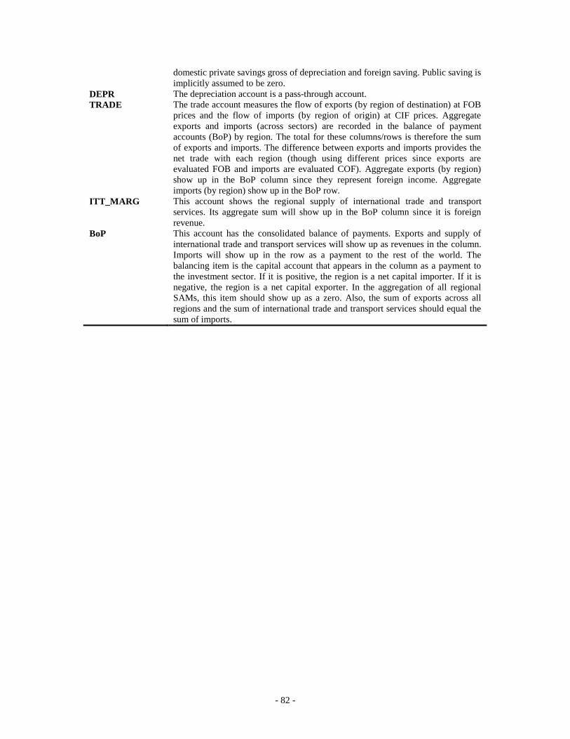
- 82 -
domestic private savings gross of depreciation and foreign saving. Public saving is
implicitly assumed to be zero.
DEPR The depreciation account is a pass-through account.
TRADE The trade account measures the flow of exports (by region of destination) at FOB
prices and the flow of imports (by region of origin) at CIF prices. Aggregate
exports and imports (across sectors) are recorded in the balance of payment
accounts (BoP) by region. The total for these columns/rows is therefore the sum
of exports and imports. The difference between exports and imports provides the
net trade with each region (though using different prices since exports are
evaluated FOB and imports are evaluated COF). Aggregate exports (by region)
show up in the BoP column since they represent foreign income. Aggregate
imports (by region) show up in the BoP row.
ITT_MARG This account shows the regional supply of international trade and transport
services. Its aggregate sum will show up in the BoP column since it is foreign
revenue.
BoP This account has the consolidated balance of payments. Exports and supply of
international trade and transport services will show up as revenues in the column.
Imports will show up in the row as a payment to the rest of the world. The
balancing item is the capital account that appears in the column as a payment to
the investment sector. If it is positive, the region is a net capital importer. If it is
negative, the region is a net capital exporter. In the aggregation of all regional
SAMs, this item should show up as a zero. Also, the sum of exports across all
regions and the sum of international trade and transport services should equal the
sum of imports.

- 83 -
Figure A8-2: The schematic Social Accounting Matrix
ACT COMM DAP MAP DIT MIT
j j j j j j
Activities i , ,( )r j r jDiag PP XP
Produced
commodities i , ,( )r j r jDiag PD XDT
, ,( )r j r jDiag PMT XMT
Domestic commodities
i , , ,r i r i jPD XD
Imported
commodities i , , ,r i r i jPMT XM
Sales tax on
dom. goods i , , , , ,
Ad
r i j r i r i jPD XD
Sales tax on
imp. goods i , , , , ,
Am
r i j r i r i jPMT XM
Value added fp , , , ,r fp j r fp jNPF XF
Value added
tax fp , , , , , ,
v
r fp j r fp j r fp jNPF XF
Production tax 1 , , ,
p
r j r j r jPX XP
Import tariffs r' ', , ', , ', ,
m
r r j r r j r r jWPM WTF
Export taxes r' , ', , ', , ',
e
r r j r r j r r jPE WTF
Households 1
Government 1 , , , , ,
Ad
r j a r j r j a
a
PD XD , , , , ,
Am
r j a r j r j a
a
PMT XM
Investment 1
Depreciation 1
Trade r' ', , ', ,r r j r r jWPM WTF
International
trade margins 1
Balance of
payments 1

- 84 -
Figure A8-2: The schematic Social Accounting Matrix, continued
VA VA_TAX PTAX EXP_TAX IMP_TAX HH
fp fp 1 r' r' 1
Activities i
Produced
commodities i
Domestic commodities
i , , ,r i r i hPD XD
Imported
commodities i , , ,r i r i hPMT XM
Sales tax on
dom. goods i , , , , ,
Ad
r i h r i r i hPD XD
Sales tax on
imp. goods i , , , , ,
Am
r i h r i r i hPMT XM
Value added fp
Value added
tax fp
Production tax 1
Import tariffs r'
Export taxes r'
Households 1 , , , ,r fp j r fp j
j
NPF XF
Government 1 , , , , , ,
v
r fp j r fp j r fp j
j
NPF XF , , ,
p
r j r j r j
j
PX XP , ', , ', , ',
e
r r i r r i r r i
i
PE WTF ', , ', , ', ,
m
r r i r r i r r i
i
WPM WTF r
hhr
cr YH,
Investment 1 h
hrS ,
Depreciation 1 rDEPRY
Trade r'
International trade margins
1
Balance of payments
1

- 85 -
Figure A8-2: The schematic Social Accounting Matrix, continued
GOV INV DEPR TRADE ITT_MARG BOP
1 1 1 r' 1 1
Activities i
Produced
commodities i , ', , ',r r i r r iWPE WTF
, ,r i r iPP XMG
Domestic commodities
i , , ,r i r i GovPD XD , , ,r i r i InvPD XD
Imported
commodities i , , ,r i r i GovPMT XM
, , ,r i r i InvPMT XM
Sales tax on
dom. goods i , , , , ,
Ad
r i Gov r i r i GovPD XD , , , , ,
Ad
r i Inv r i r i InvPD XD
Sales tax on
imp. goods i , , , , ,
Am
r i Gov r i r i GovPMT XM , , , , ,
Am
r i Inv r i r i InvPMT XM
Value added fp
Value added
tax fp
Production tax 1
Import tariffs r'
Export taxes r'
Households 1
Government 1
Investment 1 grS DEPRY f
rS
Depreciation 1
Trade r' , ', , ',r r i r r i
i
WPE WTF
International
trade margins 1 , ,r i r i
i
PP XMG
Balance of
payments 1 ', , ', ,r r j r r j
i
WPM WTF
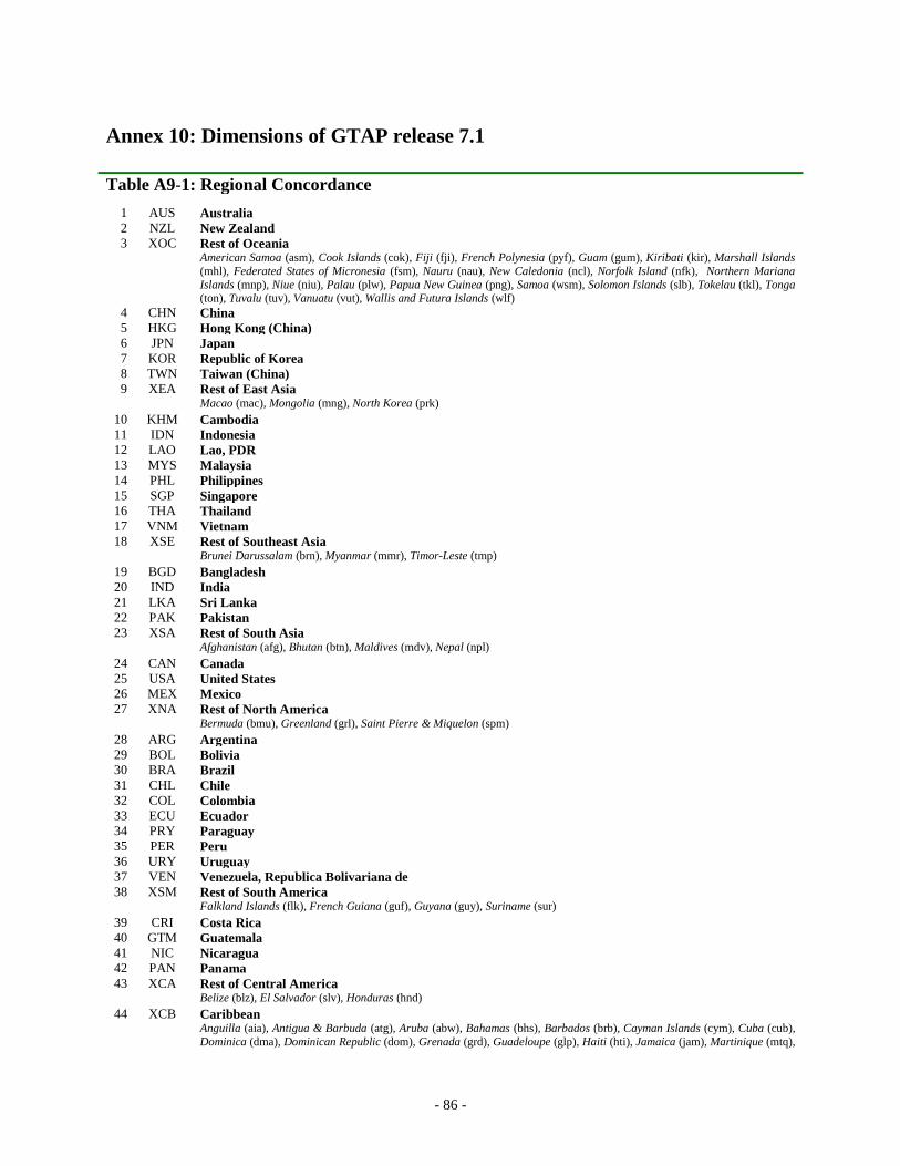
- 86 -
Annex 10: Dimensions of GTAP release 7.1
Table A9-1: Regional Concordance
1 AUS Australia
2 NZL New Zealand
3 XOC Rest of Oceania
American Samoa (asm), Cook Islands (cok), Fiji (fji), French Polynesia (pyf), Guam (gum), Kiribati (kir), Marshall Islands
(mhl), Federated States of Micronesia (fsm), Nauru (nau), New Caledonia (ncl), Norfolk Island (nfk), Northern Mariana
Islands (mnp), Niue (niu), Palau (plw), Papua New Guinea (png), Samoa (wsm), Solomon Islands (slb), Tokelau (tkl), Tonga (ton), Tuvalu (tuv), Vanuatu (vut), Wallis and Futura Islands (wlf)
4 CHN China
5 HKG Hong Kong (China)
6 JPN Japan
7 KOR Republic of Korea
8 TWN Taiwan (China)
9 XEA Rest of East Asia
Macao (mac), Mongolia (mng), North Korea (prk)
10 KHM Cambodia
11 IDN Indonesia
12 LAO Lao, PDR
13 MYS Malaysia
14 PHL Philippines
15 SGP Singapore
16 THA Thailand
17 VNM Vietnam
18 XSE Rest of Southeast Asia
Brunei Darussalam (brn), Myanmar (mmr), Timor-Leste (tmp)
19 BGD Bangladesh
20 IND India
21 LKA Sri Lanka
22 PAK Pakistan
23 XSA Rest of South Asia
Afghanistan (afg), Bhutan (btn), Maldives (mdv), Nepal (npl)
24 CAN Canada
25 USA United States
26 MEX Mexico
27 XNA Rest of North America
Bermuda (bmu), Greenland (grl), Saint Pierre & Miquelon (spm)
28 ARG Argentina
29 BOL Bolivia
30 BRA Brazil
31 CHL Chile
32 COL Colombia
33 ECU Ecuador
34 PRY Paraguay
35 PER Peru
36 URY Uruguay
37 VEN Venezuela, Republica Bolivariana de
38 XSM Rest of South America
Falkland Islands (flk), French Guiana (guf), Guyana (guy), Suriname (sur)
39 CRI Costa Rica
40 GTM Guatemala
41 NIC Nicaragua
42 PAN Panama
43 XCA Rest of Central America
Belize (blz), El Salvador (slv), Honduras (hnd)
44 XCB Caribbean
Anguilla (aia), Antigua & Barbuda (atg), Aruba (abw), Bahamas (bhs), Barbados (brb), Cayman Islands (cym), Cuba (cub),
Dominica (dma), Dominican Republic (dom), Grenada (grd), Guadeloupe (glp), Haiti (hti), Jamaica (jam), Martinique (mtq),

- 87 -
Montserrat (msr), Netherlands Antilles (ant), Puerto Rico (pri), Saint. Kitts & Nevis (kna), Saint Lucia (lca), Saint. Vincent
and the Grenadines (vct), Trinidad & Tobago (tto), Turks and Caicos Islands (tca), British Virgin Islands(vgb), United States Virgin Islands (vir)
45 AUT Austria
46 BEL Belgium
47 BGR Bulgaria
48 CYP Cyprus
49 CZE Czech Republic
50 DNK Denmark
51 EST Estonia
52 FIN Finland
53 FRA France
54 DEU Germany
55 GRC Greece
56 HUN Hungary
57 IRL Ireland
58 ITA Italy
59 LVA Latvia
60 LTU Lithuania
61 LUX Luxembourg
62 MLT Malta
63 NLD Netherlands
64 POL Poland
65 PRT Portugal
66 ROU Romania
67 SVK Slovakia
68 SVN Slovenia
69 ESP Spain
70 SWE Sweden
71 GBR United Kingdom
72 NOR Norway
73 CHE Switzerland
74 XEF Rest of European Free Trade Area (EFTA)
Iceland (isl), Liechtenstein (lei)
75 ALB Albania
76 BLR Belarus
77 HRV Croatia
78 RUS Russian Federation
79 UKR Ukraine
80 XEE Rest of Eastern Europe
Moldova (mda)
81 XER Rest of Europe
Andorra (and), , Bosnia and Herzegovina (bih), Faroe Islands (fro), Gibraltar (gib), Macedonia (mkd, former Yugoslav
Republic of), Monaco (mco), San Marino (smr), Serbia and Montenegro (scg)
82 KAZ Kazakhstan
83 KGZ Kyrgyz Republic
84 XSU Rest of Former Soviet Union
Tajikistan (tjk), Turkmenistan (tkm), Uzbekistan (uzb)
85 ARM Armenia
86 AZE Azerbaijan
87 GEO Georgia
88 IRN Iran
89 TUR Turkey
90 XWS Rest of Western Asia
Bahrain (bhr), Iraq (irq), Israel (isr), Jordan (jor), Kuwait (kwt), Lebanon (lbn), West Bank and Gaza (pse), Oman (omn),
Qatar (qat), Saudi Arabia (sau), Syrian Arab Republic (syr), United Arab Emirates (are), Republic of Yemen (yem)
91 EGY Egypt
92 MAR Morocco
93 TUN Tunisia
94 XNF Rest of North Africa
Algeria (dza), Libyan Arab Jamahiriya (lby)
95 NGA Nigeria
96 SEN Senegal

- 88 -
97 XWF Rest of Western Africa
Benin (ben), Burkina Faso (bfa), Cape Verde (cpv), Côte d'Ivoire (civ), Gambia, The (gmb), Ghana (gha), Guinea (gin),
Guinea-Bissau (gnb), Liberia (lbr), Mali (mli), Mauritania (mrt), Niger (ner), Saint Helena (shn), Sierra Leone (sle), Togo
(tgo)
98 XCF Central Africa
Cameroon (cmr), Central African Republic (caf), Chad (tcd), Congo (cog), Equatorial Guinea (gnq), Gabon (gab), Sao
Tome & Principe (stp)
99 XAC South-Central Africa
Angola (ago), Democratic Republic of the Congo (cod, formerly Zaïre)
100 ETH Ethiopia
101 MDG Madagascar
102 MWI Malawi
103 MUS Mauritius
104 MOZ Mozambique
105 TZA Tanzania
106 UGA Uganda
107 ZMB Zambia
108 ZWE Zimbabwe
109 XEC Rest of Eastern Africa
Burundi (bdi), Comoros (com), Djibouti (dji), Eritrea (eri), Kenya (ken), Mayotte (myt), Réunion (reu), Rwanda (rwa), Seychelles Islands (syc), Somalia (som), Sudan (sdn)
110 BWA Botswana
111 ZAF South Africa
112 XSS Rest of South African Customs Union Lesotho (lso), Namibia (nam),Swaziland (swz)
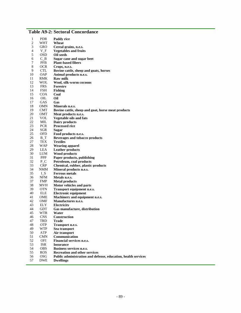
- 89 -
Table A9-2: Sectoral Concordance
1 PDR Paddy rice 2 WHT Wheat 3 GRO Cereal grains, n.e.s. 4 V_F Vegetables and fruits 5 OSD Oil seeds 6 C_B Sugar cane and sugar beet 7 PFB Plant-based fibers 8 OCR Crops, n.e.s. 9 CTL Bovine cattle, sheep and goats, horses
10 OAP Animal products n.e.s. 11 RMK Raw milk 12 WOL Wool, silk-worm cocoons 13 FRS Forestry 14 FSH Fishing 15 COA Coal 16 OIL Oil 17 GAS Gas 18 OMN Minerals n.e.s. 19 CMT Bovine cattle, sheep and goat, horse meat products 20 OMT Meat products n.e.s. 21 VOL Vegetable oils and fats 22 MIL Dairy products 23 PCR Processed rice 24 SGR Sugar 25 OFD Food products n.e.s. 26 B_T Beverages and tobacco products 27 TEX Textiles 28 WAP Wearing apparel 29 LEA Leather products 30 LUM Wood products 31 PPP Paper products, publishing 32 P_C Petroleum, coal products 33 CRP Chemical, rubber, plastic products 34 NMM Mineral products n.e.s. 35 I_S Ferrous metals 36 NFM Metals n.e.s. 37 FMP Metal products 38 MVH Motor vehicles and parts 39 OTN Transport equipment n.e.s. 40 ELE Electronic equipment 41 OME Machinery and equipment n.e.s. 42 OMF Manufactures n.e.s. 43 ELY Electricity 44 GDT Gas manufacture, distribution 45 WTR Water 46 CNS Construction 47 TRD Trade 48 OTP Transport n.e.s. 49 WTP Sea transport 50 ATP Air transport 51 CMN Communication 52 OFI Financial services n.e.s. 53 ISR Insurance 54 OBS Business services n.e.s. 55 ROS Recreation and other services 56 OSG Public administration and defense, education, health services 57 DWE Dwellings

- 90 -
Figures
Figure 1: Production structure nesting
Output (XP)
Total non-energy intermediate demand (ND)
Value added plus energy demand (VA)
Non-energy intermediate demand (XA)
By region of origin—domestic (XD) and
imported (WTF)
Demand for labor, land and sector
specific factors (XFfpx)
Demand for capital and energy (KE)
Demand for capital by
vintage (KV)
Demand for energy bundle
(XNRG)
See figure 2
p
n
v
v
f
ke
f
n

- 91 -
Figure 2: Energy nesting
Energy bundle (XNRG)
Gas bundle (XGAS)
Electric bundle (XELY)
Non-electric bundle (XNELY)
Coal bundle (XCOA)
Oil and gas bundle (XONG)
Oil bundle (XOIL)
Conventional (ely) and alternative technologies
Conventional (coa) and alternative technologies
Conventional (gas & gdt) and alternative technologies
e
nely
olg
ely
coa
gas
oil
Conventional (oil & p_c) and alternative technologies

- 92 -
Figure 3: Output, supply and trade
Output (XP)
Supply (XS)
Domestic sales (XDs) Aggregate exports (XET)
Armington demand (XAT)
Bilateral export supply (WTFs)
Domestic demand (XDd) Aggregate imports (XMT)
Bilateral import demand (WTFd)
Equilibrium domestic price
(PD) Equilibrium trade
price (WPE)
s
x
z
m
w

- 93 -
Figure 4: Domestic demand nesting
The allocation of national income across expenditure categories is determined by the closure
rules. By default all net factor income accrues to households. Households allocate their
disposable income between savings and expenditures on goods and services. The savings
function depends on a number of factors including demographic variables. Public expenditures
are fixed as a share of nominal GDP. Investment expenditures are constrained by available
savings—household, public (normally set at zero) and foreign. The default household demand
specification is the CDE, but the model includes the ELES and AIDADS as well.
National income (Y)
Public expenditures
(YG)
Investment expenditures
(YS)
Private expenditures
(YH)
Armington demand Armington demand
f
f
Demand for consumer goods
(HXk)
Constant difference in
elasticities (CDE)
Non-energy Armington
demand (XAi)
Energy demand (XNRG)
See figure 2
c CES-based
transition matrix


![Welcome [siteresources.worldbank.org]siteresources.worldbank.org/.../7-e-GPinGoAP-Bikshapathy-11106.pdf · Welcome to Presentation on e-GP: Govt of AP Experience K.Bikshapathi, Project](https://img.dokumen.tips/doc/110x75/5b419a1c7f8b9af9638ba3b0/welcome-welcome-to-presentation-on-e-gp-govt-of-ap-experience-kbikshapathi.jpg)


