THE ENCODING AND FOURIER DESCRIPTORS OF ...ufdcimages.uflib.ufl.edu/UF/00/10/07/51/00001/Thesis_ETD.pdfTHE ENCODING AND FOURIER DESCRIPTORS OF ARBITRARY CURVES IN 3-DIMENSIONAL SPACE

THE ENCODING AND FOURIER DESCRIPTORS OF ARBITRARY CURVESIN 3-DIMENSIONAL SPACE

By

PAROMITA BOSE

A THESIS PRESENTED TO THE GRADUATE SCHOOLOF THE UNIVERSITY OF FLORIDA IN PARTIAL FULFILLMENT

OF THE REQUIREMENTS FOR THE DEGREE OFMASTER OF SCIENCE

UNIVERSITY OF FLORIDA

2000

Dedicated to my parents

and

my husband Andrew

ACKNOWLEDGMENTS

First, my heartfelt thanks and appreciation go to my advisor, Dr. Gerhard X.

Ritter, for his kind help and patience in guiding me through the preparation of this

thesis. His insight and support are deeply appreciated. Working with him was an

honor for me. I would also like to thank Drs. Dankel and Chen, for taking the time

to read this thesis and to serve on my supervisory committee.

Finally, I would like to thank my parents and my husband, Andrew, for their

encouragement, guidance, and support without which I would not have accomplished

this work.

iii

TABLE OF CONTENTS

ACKNOWLEDGEMENTS . . . . . . . . . . . . . . . . . . . . . . . . . . . . iii

ABSTRACT . . . . . . . . . . . . . . . . . . . . . . . . . . . . . . . . . . . . v

CHAPTERS

1 INTRODUCTION . . . . . . . . . . . . . . . . . . . . . . . . . . . . . 1

2 BACKGROUND OVERVIEW . . . . . . . . . . . . . . . . . . . . . . 4

2.1 Chain Codes . . . . . . . . . . . . . . . . . . . . . . . . . . . . . 42.2 Fourier Descriptors . . . . . . . . . . . . . . . . . . . . . . . . . 7

3 CHAIN CODES OF ARBITRARY CURVES IN 3D . . . . . . . . . . 9

3.1 The Encoding Process . . . . . . . . . . . . . . . . . . . . . . . . 93.2 The Encoding Algorithm . . . . . . . . . . . . . . . . . . . . . . 133.3 Elementary Manipulations . . . . . . . . . . . . . . . . . . . . . 19

4 FOURIER DESCRIPTORS FOR THE 3D CHAIN CODE . . . . . . 27

4.1 Fourier coefficients of the chain code in 3D . . . . . . . . . . . . 274.2 Normalization of the Fourier coefficients for the 3D chain code . 34

5 CONCLUSIONS AND FUTURE WORK . . . . . . . . . . . . . . . . 39

APPENDIXES

A IMPLEMENTATION OF THE 3D CHAIN CODE . . . . . . . . . . 40

B IMPLEMENTATION OF THE FOURIER DESCRIPTORS . . . . . . 78

REFERENCES . . . . . . . . . . . . . . . . . . . . . . . . . . . . . . . . . . . 87

BIOGRAPHICAL SKETCH . . . . . . . . . . . . . . . . . . . . . . . . . . . . 90

iv

Abstract of Thesis Presented to the Graduate Schoolof the University of Florida in Partial Fulfillment of the

Requirements for the Degree of Master of Science

THE ENCODING AND FOURIER DESCRIPTORS OF ARBITRARY CURVESIN 3-DIMENSIONAL SPACE

By

Paromita Bose

December 2000

Chairman: Dr. Gerhard X. RitterMajor Department: Computer and Information Science and Engineering

The increasing importance of three-dimensional shape analysis and pattern

recognition in medical imaging, target classification, image sequence analysis, shape

matching, robotic navigation and other domains necessitates the need for a cod-

ing scheme which is universally applicable to arbitrary types of digitized curves,

extremely simple, highly standardized, and capable of facilitating computer manipu-

lation and analysis of curve properties.

In this work, we describe a simple and efficient scheme for encoding digitized

1-dimensional curves in 3D. Using this scheme, we develop an algorithm for accurately

encoding any digital 1-dimensional curve embedded in 3D-space. Additionally, we

develop Fourier Descriptors for the 3D chain code in order to reconstruct the curve.

We also present an intuitive and mathematically pleasing technique of normalizing

the Fourier Descriptors in order to make the contour representation invariant with

respect to rotation, dilation, translation and the starting point of the contour.

v

CHAPTER 1INTRODUCTION

The study of arbitrary curve representations in 3-dimensional space is an im-

portant part of computer vision. Chain code techniques are widely used because

they preserve information and allow considerable data reduction. Chain codes are

the standard input format for numerous shape analysis and pattern recognition al-

gorithms.

In order to analyze, synthesize and manipulate arbitrary curves embedded in

3-dimensional space, the need arises for precise means of describing these curves.

In consideration of computational time and memory space requirements, it is often

desirable to convert the arbitrary curve into a representative form that can be ef-

ficiently processed. Contour representation is one of the most popular forms. For

example, if one wishes to transmit the contour of an airplane over a communica-

tion link, the contour must first be described and encoded in a fashion that permits

efficient transmission. The decoding at the receiving end should permit a faithful

pictorial reconstruction of the airplane’s contour.

The first approach for representing digital curves using chain codes was in-

troduced by Freeman in 1961 [10]. It was developed with the aim of making image

processing and analysis simpler. The chain code moves along a sequence of bor-

der pixels based on a 4- or 8- connectivity. The direction of each movement is

encoded using a numbering scheme, such as {i|i = 0, 1, ..., 7}, denoting an angle of

45i counter-clockwise from the positive axis. The chain codes can be viewed as a

connected sequence of straight line segments with specified lengths and directions.

1

2

Many authors have since then been using techniques of chain coding due to the

fact that various shape features may be computed directly from this representation

[2, 4, 18, 21, 24, 25, 31].

In this work, we describe a simple and efficient scheme for encoding digitized 1-

dimensional curves in 3D. Using this scheme, we develop an algorithm for accurately

encoding any digital 1-dimensional curve embedded in 3-space. Additionally, we

develop Fourier Descriptors for the 3D chain code in order to reconstruct the curve.

We also present a mathematically pleasing technique for normalizing the Fourier

descriptors of the 3D chain code, in order to make the contour representation invariant

with respect to rotation, dilation, translation and the starting point of the contour.

The work on Fourier Descriptors is an extension of the work of Kuhl and Giardina

[20] to 3D.

Some of the important applications of the chain code have been in pattern

recognition problems, and many have become standard techniques. Shape matching

[7, 8], computer recognition of curved objects [23, 24], motion analysis [5, 22], con-

nectivity analysis [27, 29], straight line determination [30] and target classification

are but a few of these applications. Fourier Descriptors [19, 20] for describing closed

contours based on the chain code have direct applications to a wide variety of pattern

recognition problems that involve analysis of well-defined image contours.

The remainder of this thesis is organized as follows:

Chapter 2 presents an overview of the related work done in this area. In

Chapter 3, we describe the encoding scheme and the chain coding algorithm for

arbitrary curves in 3D. Some elementary manipulations for the 3D chain code have

also been suggested. In Chapter 4, we present the Fourier Descriptors for the 3D

chain code and the results obtained after applying them to digitized 1-dimensional

curves in 3D. We also present an intuitively pleasing way of normalizing the Fourier

3

coefficients for the chain code in 3D. Chapter 5 concludes the thesis and presents

some open problems for future work.

CHAPTER 2BACKGROUND OVERVIEW

2.1 Chain Codes

Chain codes are used to represent a boundary by a connected sequence of

straight line segments of specified length and direction.

Since digital images are usually acquired and processed in a grid format with

equal spacing in the x and y directions (x,y and z in 3D), one could generate a chain

code by following the boundary of a connected object in, say, a clockwise direction and

assigning a direction to the segments connecting every pair of boundary pixels. This

is generally unacceptable for two principal reasons: first, the resulting chain code

will usually be quite long and second, any small disturbances along the boundary

due to noise or imperfect segmentation will cause changes in the code that may not

necessarily be related to the shape of the boundary.

An approach frequently used to circumvent the problem discussed above is to

“resample” the boundary by selecting a larger grid spacing, as illustrated in Figure

2.1(a). Then as the boundary is traversed, we assign a boundary point to each node

of the large grid depending on the proximity of the original boundary to that node as

shown in Figure 2.1(b). The resampled boundary can then be encoded as shown in

Figure 2.2. As might be expected, the accuracy of the resulting code representation

depends on the spacing of the sampling grid. Various digitization schemes have been

suggested in references [15, 17, 32].

Freeman [10, 12] showed that line structures in 2D can be characterized by

the property that each data node in sequence coincides with one of eight grid nodes

that surround the previous data node. In the Freeman chain code, the eight digits

0 through 7 are assigned to the eight possible directions leading from one data node

4

5

(a) (b)

Figure 2.1: A digitized curve in 2D (a) Digital boundary with resampling grid super-imposed. (b) Result of resampling

2

1

2

3

3 5

5

6

6

6

6

70

2

1

(c)

Figure 2.2: Freeman chain code of the digitized curve in Figure 2.1(b)

6

0

2

3

4

5

6

7

1

Figure 2.3: 8-directions of the Freeman chain code

to the next as shown in Figure 2.3. Each chain code direction can thus be encoded

using 3 bits. Each octal digit corresponds to one directed straight line segment which

is referred to as a link. A sequence of links representing a line structure is called

a chain [10, 12]. Freeman [10] showed that under the assumption of a sufficiently

fine quantization, the changes in directions from link to link will normally not exceed

±45◦. Turns of ±90◦ will be infrequent and turns in excess of 90◦, most rare.

Other coding schemes have been developed for representing irregular line

structures in 2D. Some of these are simply variations of the octagonal chain code

[18, 31], some are more compact representations [9] and some have features that make

them attractive for particular processing applications. A comprehensive tutorial re-

view of techniques for computer processing of line drawing images in 2 dimensions is

presented in the paper by Freeman [12].

For many years, authors have paid more attention to 3D shape description

algorithms using contour information per se than to the problem of chain code repre-

sentations. Cohen and Wang [6] describe 3D object recognition and shape estimation

7

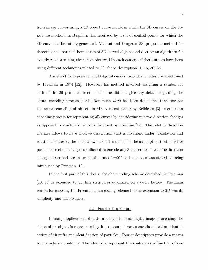
from image curves using a 3D object curve model in which the 3D curves on the ob-

ject are modeled as B-splines characterized by a set of control points for which the

3D curve can be totally generated. Vaillant and Faugeras [33] propose a method for

detecting the extremal boundaries of 3D curved objects and decribe an algorithm for

exactly reconstructing the curves observed by each camera. Other authors have been

using different techniques related to 3D shape description [1, 16, 30, 36].

A method for representing 3D digital curves using chain codes was mentioned

by Freeman in 1974 [12]. However, his method involved assigning a symbol for

each of the 26 possible directions and he did not give any details regarding the

actual encoding process in 3D. Not much work has been done since then towards

the actual encoding of objects in 3D. A recent paper by Bribiesca [3] describes an

encoding process for representing 3D curves by considering relative direction changes

as opposed to absolute directions proposed by Freeman [12]. The relative direction

changes allows to have a curve description that is invariant under translation and

rotation. However, the main drawback of his scheme is the assumption that only five

possible direction changes is sufficient to encode any 3D discrete curve. The direction

changes described are in terms of turns of ±90◦ and this case was stated as being

infrequent by Freeman [12].

In the first part of this thesis, the chain coding scheme described by Freeman

[10, 12] is extended to 3D line structures quantized on a cubic lattice. The main

reason for choosing the Freeman chain coding scheme for the extension to 3D was its

simplicity and effectiveness.

2.2 Fourier Descriptors

In many applications of pattern recognition and digital image processing, the

shape of an object is represented by its contour: chromosome classification, identifi-

cation of aircrafts and identification of particles. Fourier descriptors provide a means

to characterize contours. The idea is to represent the contour as a function of one

8

variable, expand the function in terms of its Fourier series, and use the coefficients

of the series as Fourier Descriptors (FDs).

Fourier Descriptors have been successfully used by many investigators [13, 20,

26, 34, 35]. The work of Kuhl and Giardina [20] deserves special mention. They

described a particularly simple way of obtaining the Fourier coefficients of a Freeman

encoded closed contour in 2D. The resulting Fourier Descriptors are invariant with

respect to rotation, dilation and translation of the contour, and lose no information

about the shape of the contour.

In the second part of this thesis, the method of Fourier Descriptors obtained

by Kuhl and Giardina [20] is extended to arbitrary curves in 3D.

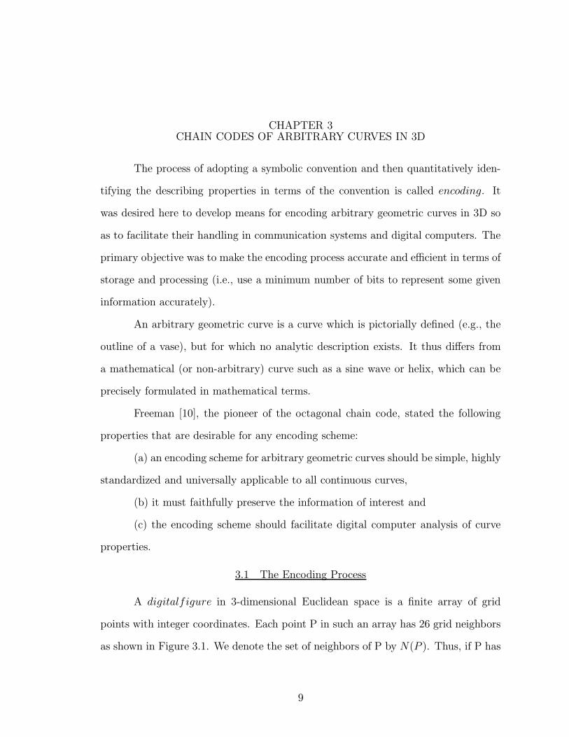
CHAPTER 3CHAIN CODES OF ARBITRARY CURVES IN 3D

The process of adopting a symbolic convention and then quantitatively iden-

tifying the describing properties in terms of the convention is called encoding. It

was desired here to develop means for encoding arbitrary geometric curves in 3D so

as to facilitate their handling in communication systems and digital computers. The

primary objective was to make the encoding process accurate and efficient in terms of

storage and processing (i.e., use a minimum number of bits to represent some given

information accurately).

An arbitrary geometric curve is a curve which is pictorially defined (e.g., the

outline of a vase), but for which no analytic description exists. It thus differs from

a mathematical (or non-arbitrary) curve such as a sine wave or helix, which can be

precisely formulated in mathematical terms.

Freeman [10], the pioneer of the octagonal chain code, stated the following

properties that are desirable for any encoding scheme:

(a) an encoding scheme for arbitrary geometric curves should be simple, highly

standardized and universally applicable to all continuous curves,

(b) it must faithfully preserve the information of interest and

(c) the encoding scheme should facilitate digital computer analysis of curve

properties.

3.1 The Encoding Process

A digitalfigure in 3-dimensional Euclidean space is a finite array of grid

points with integer coordinates. Each point P in such an array has 26 grid neighbors

as shown in Figure 3.1. We denote the set of neighbors of P by N(P ). Thus, if P has

9

10

24 2523

22

21 20 19

18

171615

14

13 12 11

10

9

8

p

765

4

3 2 1

0

Figure 3.1: The 26-neighbors of a point p

coordinates (i, j, k), then

N(P ) = {(x, y, z) : 0 < [(i− x)2 + (j − y)2 + (k − z)2]1

2 ≤√3} and x,y,z ∈ Z

where Z denotes the set of integers.

For any point P (x, y, z) in a 3-dimensional digital figure, our approach uses

the symbols in Table 3.1 to denote the directions that can be directly approached

from point P.

The novelty of our encoding scheme is the idea that 26 directions can be

encoded using only 12 symbols viz. 0, 1, 2, 3, 4, 5, 6, 7, i,−i, j, and −j. This lends

a very natural and logical meaning to the 26 chain code directions. Points in the

XY-plane are chain coded using the 8 Freeman chain code directions from 0 through

7. i and −i correspond to the directions to reach points in the planes directly above

and directly below the XY-plane respectively. j and −j are used to reach points

that are diagonally located from a point in the XY-plane. For example, j0 denotes

“moving vertically up along the positive Z-direction followed by a movement along

the 0 direction in the same plane”.

11

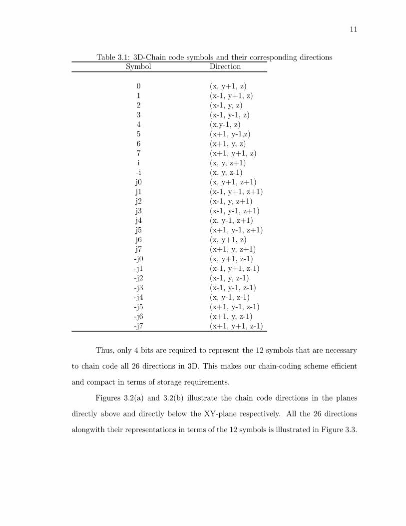
Table 3.1: 3D-Chain code symbols and their corresponding directionsSymbol Direction

0 (x, y+1, z)1 (x-1, y+1, z)2 (x-1, y, z)3 (x-1, y-1, z)4 (x,y-1, z)5 (x+1, y-1,z)6 (x+1, y, z)7 (x+1, y+1, z)i (x, y, z+1)-i (x, y, z-1)j0 (x, y+1, z+1)j1 (x-1, y+1, z+1)j2 (x-1, y, z+1)j3 (x-1, y-1, z+1)j4 (x, y-1, z+1)j5 (x+1, y-1, z+1)j6 (x, y+1, z)j7 (x+1, y, z+1)-j0 (x, y+1, z-1)-j1 (x-1, y+1, z-1)-j2 (x-1, y, z-1)-j3 (x-1, y-1, z-1)-j4 (x, y-1, z-1)-j5 (x+1, y-1, z-1)-j6 (x+1, y, z-1)-j7 (x+1, y+1, z-1)

Thus, only 4 bits are required to represent the 12 symbols that are necessary

to chain code all 26 directions in 3D. This makes our chain-coding scheme efficient

and compact in terms of storage requirements.

Figures 3.2(a) and 3.2(b) illustrate the chain code directions in the planes

directly above and directly below the XY-plane respectively. All the 26 directions

alongwith their representations in terms of the 12 symbols is illustrated in Figure 3.3.

12

5 6

0

123

4

7

i

j2

j0

j1j3

j4

j5 j6 j7

p

−j1

p0

123

4

5 6 7

−j0

−j2−j3

−j4

−j5−j7−j6

(a) (b)

−i

Figure 3.2: 3D-chain code directions (a) Chain code directions in the XY-plane andthe plane directly above it (b) Chain code directions in the XY-plane and the planedirectly below it

Y

X

Z

j0

7

−j3

6

−j7−j6−j5

−j4

−j2 −j1

−j0

j7j6j5

j4

j3 j2 j1

−i

i

p

5

4

3

0

12

Figure 3.3: The 26 directions of the 3D-chain code

13

Let π be anM x N xK array of grid points having positive integer coordinates

(m,n, k) where 1 ≤ k ≤ K. Let C be a digitized one-dimensional curve embedded in

3D. The process of chain coding C is as follows:

We scan the array π for a starting point of C say, S. Then we scan for a

second point, chain code the direction and proceed to search for the next point, and

so on. The process stops when one reaches back to the starting point S.

The idea of the encoding process is quite simple but it involves several book-

keeping chores, such as keeping track of points already visited and tracing over pre-

vious parts. The next section describes the 3D chain coding algorithm in detail.

3.2 The Encoding Algorithm

To be more precise, we shall now summarize the encoding process into algo-

rithmic form and present some examples.

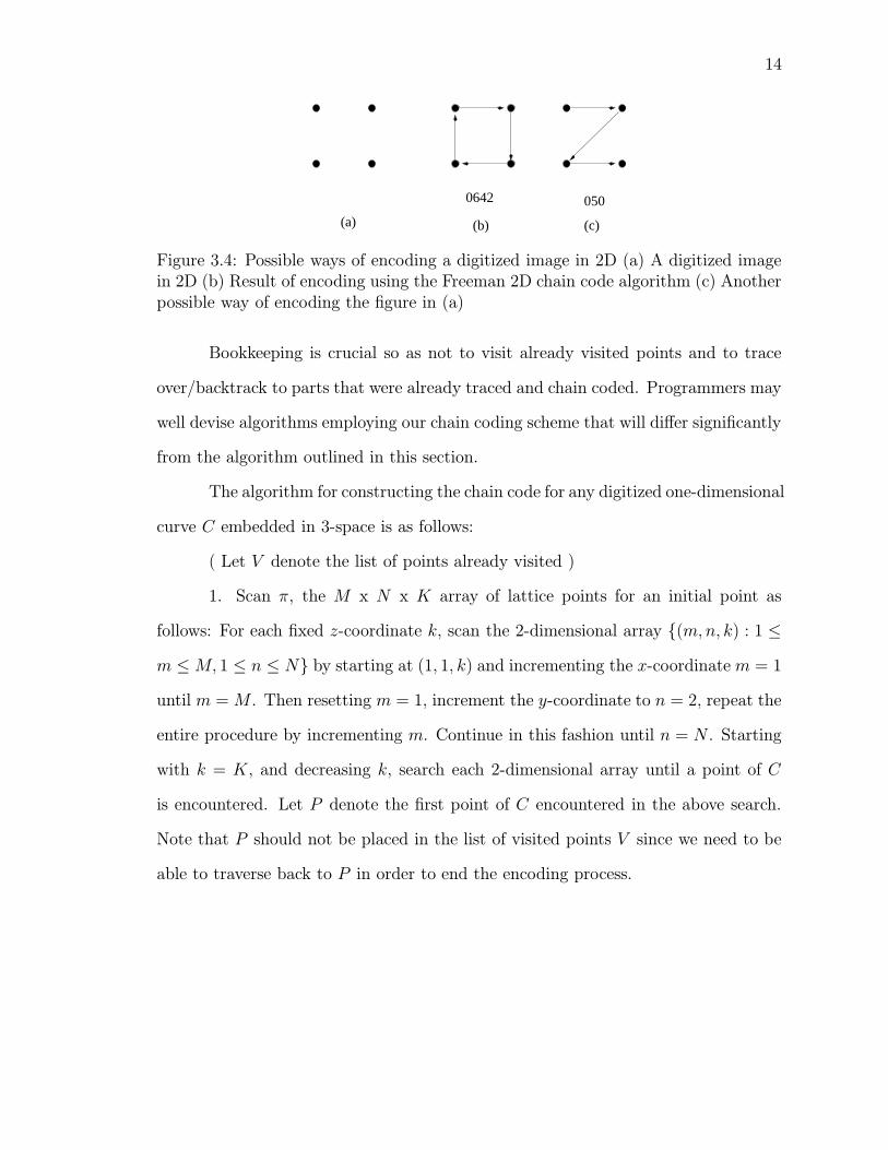
As in Freeman’s octagonal chain code, there are ambiguities that must be

overcome when writing an algorithm for encoding a contour in 3D. For example, the

configuration in Figure 3.4(a), could be encoded as the polygonal curve 0642 or 050,

as shown in Figures 3.4(b) and (c) respectively. In order to obtain an unambiguous

algorithm, rules have to be defined which determine how one is to proceed from a

given point to the next. A standard approach described by Freeman is to search

a binary array from left to right, starting with the topmost row and continuing

downward, until the first non-zero entry is encountered. From then on, the search for

the next non-zero entry proceeds in a clockwise fashion starting at the neighboring

point 135◦ from the last given direction and point and proceeding clockwise until the

next non-zero entry is found. The algorithm also performs several bookkeeping tasks

in the process. Under this scheme, Figure 3.4(a) would be encoded as 0642.

In general, the resulting code may not portray the actual curve represented

by the array. However, we are assured that the polygonal curve represented by the

chain code lies within a bound of unit(grid) distance of the digitized curve.

14

(c)(b)(a)

0500642

Figure 3.4: Possible ways of encoding a digitized image in 2D (a) A digitized imagein 2D (b) Result of encoding using the Freeman 2D chain code algorithm (c) Anotherpossible way of encoding the figure in (a)

Bookkeeping is crucial so as not to visit already visited points and to trace

over/backtrack to parts that were already traced and chain coded. Programmers may

well devise algorithms employing our chain coding scheme that will differ significantly

from the algorithm outlined in this section.

The algorithm for constructing the chain code for any digitized one-dimensional

curve C embedded in 3-space is as follows:

( Let V denote the list of points already visited )

1. Scan π, the M x N x K array of lattice points for an initial point as

follows: For each fixed z-coordinate k, scan the 2-dimensional array {(m,n, k) : 1 ≤

m ≤M, 1 ≤ n ≤ N} by starting at (1, 1, k) and incrementing the x-coordinate m = 1

until m =M . Then resetting m = 1, increment the y-coordinate to n = 2, repeat the

entire procedure by incrementing m. Continue in this fashion until n = N . Starting

with k = K, and decreasing k, search each 2-dimensional array until a point of C

is encountered. Let P denote the first point of C encountered in the above search.

Note that P should not be placed in the list of visited points V since we need to be

able to traverse back to P in order to end the encoding process.

15

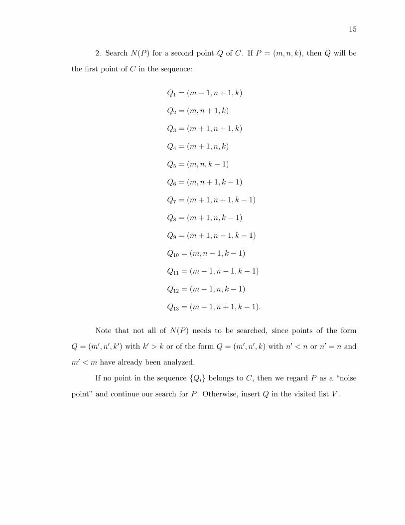
2. Search N(P ) for a second point Q of C. If P = (m,n, k), then Q will be

the first point of C in the sequence:

Q1 = (m− 1, n+ 1, k)

Q2 = (m,n + 1, k)

Q3 = (m + 1, n+ 1, k)

Q4 = (m + 1, n, k)

Q5 = (m,n, k − 1)

Q6 = (m,n + 1, k − 1)

Q7 = (m + 1, n+ 1, k − 1)

Q8 = (m + 1, n, k − 1)

Q9 = (m + 1, n− 1, k − 1)

Q10 = (m,n− 1, k − 1)

Q11 = (m− 1, n− 1, k − 1)

Q12 = (m− 1, n, k − 1)

Q13 = (m− 1, n+ 1, k − 1).

Note that not all of N(P ) needs to be searched, since points of the form

Q = (m′, n′, k′) with k′ > k or of the form Q = (m′, n′, k) with n′ < n or n′ = n and

m′ < m have already been analyzed.

If no point in the sequence {Qi} belongs to C, then we regard P as a “noise

point” and continue our search for P . Otherwise, insert Q in the visited list V .

16

3. Once P and Q have been found, we search N(P ) for a third point R by

scanning all 26 directions except in the direction from Q to P in the following order:

i, j4, j3, j2, j1, j0, j7, j6, j5,

4, 3, 2, 1, 0, 7, 6, 5,

− i,−j4,−j3,−j2,−j1,−j0,−j7,−j6,−j5.

If a point of C is found and the point does not appear in the visited list V , then

chain code the direction traversed according to the symbols in Table 3.1 and insert

the point found into the visited list V . Note that scanning along the direction from

Q to P is avoided since this may lead to a premature termination of the algorithm.

4. Search for the next point by scanning along all 26 directions from the given

point in the following order:

i, j4, j3, j2, j1, j0, j7, j6, j5,

4, 3, 2, 1, 0, 7, 6, 5,

− i,−j4,−j3,−j2,−j1,−j0,−j7,−j6,−j5.

Notice that the convention chosen here is to scan the upper plane first, then

the plane in which the point lies and finally the lower plane.

5. If a point of C is found and the point does not appear in the visited list

V , then chain code the direction traversed according to the symbols in Table 3.1 and

insert the point found into the visited list V . Repeat Step 4.

6. If no point of C is found (i.e., either the point in question has no neighbors

or no ’unvisited’ neighbors) then back track to the most recently visited point i.e.

the last point of the list V , chain code that direction and go back to Step 4.

7. The process terminates when the starting point P is reached. This is

essential in order to obtain a closed contour, which is necessary for fitting the curve

using the method of Fourier Descriptors described in Chapter 4.

17

216

−i

4

i

6

i

Starting point

(c)(b)

(a)

4

−i

x

y

z

0

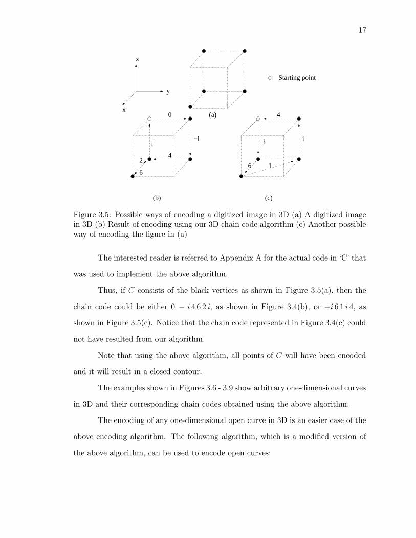
Figure 3.5: Possible ways of encoding a digitized image in 3D (a) A digitized imagein 3D (b) Result of encoding using our 3D chain code algorithm (c) Another possibleway of encoding the figure in (a)

The interested reader is referred to Appendix A for the actual code in ‘C’ that

was used to implement the above algorithm.

Thus, if C consists of the black vertices as shown in Figure 3.5(a), then the

chain code could be either 0 − i 4 6 2 i, as shown in Figure 3.4(b), or −i 6 1 i 4, as

shown in Figure 3.5(c). Notice that the chain code represented in Figure 3.4(c) could

not have resulted from our algorithm.

Note that using the above algorithm, all points of C will have been encoded

and it will result in a closed contour.

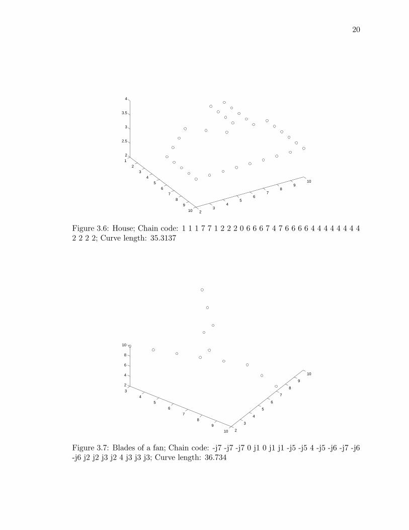
The examples shown in Figures 3.6 - 3.9 show arbitrary one-dimensional curves

in 3D and their corresponding chain codes obtained using the above algorithm.

The encoding of any one-dimensional open curve in 3D is an easier case of the

above encoding algorithm. The following algorithm, which is a modified version of

the above algorithm, can be used to encode open curves:

18

1. Scan π, the M x N x K array of lattice points for an initial point P in

the same manner as outlined in the above algorithm. Insert P into the list of visited

points V .

2. Search N(P ) for a second point Q of C. If P = (m,n, k), then Q will be

the first point of C in the sequence:

Q1 = (m− 1, n+ 1, k)

Q2 = (m,n + 1, k)

Q3 = (m + 1, n+ 1, k)

Q4 = (m + 1, n, k)

Q5 = (m,n, k − 1)

Q6 = (m,n + 1, k − 1)

Q7 = (m + 1, n+ 1, k − 1)

Q8 = (m + 1, n, k − 1)

Q9 = (m + 1, n− 1, k − 1)

Q10 = (m,n− 1, k − 1)

Q11 = (m− 1, n− 1, k − 1)

Q12 = (m− 1, n, k − 1)

Q13 = (m− 1, n+ 1, k − 1).

Note that not all of N(P ) needs to be searched, since points of the form

Q = (m′, n′, k′) with k′ > k or of the form Q = (m′, n′, k) with n′ < n or n′ = n and

m′ < m have already been analyzed.

If no point in the sequence {Qi} belongs to C, then we regard P as a “noise

point” and continue our search for P . Otherwise, insert Q in the visited list V .

19

3. Search for the next point by scanning along all 26 directions from the given

point in the following order:

i, j4, j3, j2, j1, j0, j7, j6, j5,

4, 3, 2, 1, 0, 7, 6, 5,

− i,−j4,−j3,−j2,−j1,−j0,−j7,−j6,−j5.

Notice that the convention chosen here is to scan the upper plane first, then

the plane in which the point lies and finally the lower plane.

4. If a point of C is found and the point does not appear in the visited list

V , then chain code the direction traversed according to the symbols in Table 3.1 and

insert the point found into the visited list V . Repeat Step 3.

5. The algorithm terminates when a given point either has no neighbors or

no ’unvisited’ neighbors.

Figures 3.10 - 3.11 show one-dimensional open curves in 3D and their corre-

sponding chain codes obtained using the modified algorithm.

3.3 Elementary Manipulations

Inverse Directions

Inspection of Figure 3.3 shows that directions which are diametrically opposite have

a canceling effect on each other. Accordingly, symbols representing such directions

are referred to as inverses of each other. Numerically, the inverse of a direction in

the chain code is obtained by simply adding “4” modulo 8 to a numerical digit and

switching i and −i with −i and i respectively and also switching j and −j with −j

and j respectively. For example, the inverse of “j6” will be “−j2”.

Table 3.2 lists all 26 3D-Chain code directions and their inverses.

20

12

34

56

78

910 2

34

56

78

910

2

2.5

3

3.5

4

Figure 3.6: House; Chain code: 1 1 1 7 7 1 2 2 2 0 6 6 6 7 4 7 6 6 6 6 4 4 4 4 4 4 4 42 2 2 2; Curve length: 35.3137

3

4

5

6

7

8

9

10 2

3

4

5

6

7

8

9

10

2

4

6

8

10

Figure 3.7: Blades of a fan; Chain code: -j7 -j7 -j7 0 j1 0 j1 j1 -j5 -j5 4 -j5 -j6 -j7 -j6-j6 j2 j2 j3 j2 4 j3 j3 j3; Curve length: 36.734

21

12

34

56

7

2

3

4

5

6

7

8

0

5

10

Figure 3.8: Vase; Chain code: 0 0 0 0 -j5 -j6 -j7 -j7 -j6 -j5 4 4 4 4 j3 j2 j1 j1 j2 j3;Curve length: 27.5133

0

5

10

15

02

46

810

12

4

6

8

10

12

14

16

18

Figure 3.9: Airplane; Chain code: -j7 0 0 j1 -j7 0 0 -j5 -j6 -j5 j3 -j5 -j6 -j6 -j6 -j6 -j6-j6 -j6 -j6 -j5 j3 j2 j2 j2 j2 j2 j2 j2 j2 j3 -j5 j3 j2 j3 0 0 j1; Curve length: 55.7046

22

2

3

4

5

6

34567896

6.5

7

7.5

8

8.5

9

9.5

10

Figure 3.10: Chain code: -j5 -j6 -j6 -j5 4 4 j3 j2 j2; Curve length: 12.8530

02

46

8

−3−2−10123450

5

10

15

20

25

30

Figure 3.11: Chain code: -j0 -j0 -j7 -j7 -j6 -j6 -j5 -j5 -j5 -j4 -j4 -j3 -j3 -j3 -j2 -j1 -j1-j0 -j0 -j7 -j6 -j5 -j4 -j3 -j2 -j0; Curve length: 45.4619

23

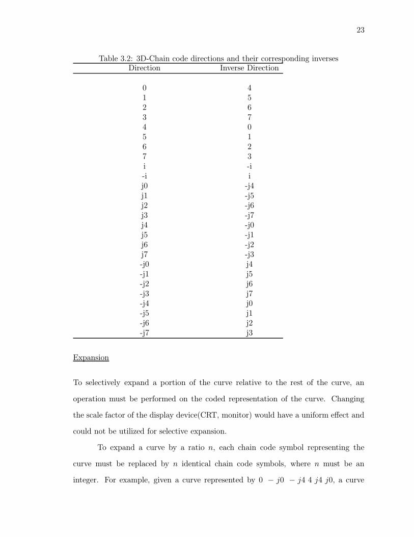
Table 3.2: 3D-Chain code directions and their corresponding inversesDirection Inverse Direction

0 41 52 63 74 05 16 27 3i -i-i ij0 -j4j1 -j5j2 -j6j3 -j7j4 -j0j5 -j1j6 -j2j7 -j3-j0 j4-j1 j5-j2 j6-j3 j7-j4 j0-j5 j1-j6 j2-j7 j3

Expansion

To selectively expand a portion of the curve relative to the rest of the curve, an

operation must be performed on the coded representation of the curve. Changing

the scale factor of the display device(CRT, monitor) would have a uniform effect and

could not be utilized for selective expansion.

To expand a curve by a ratio n, each chain code symbol representing the

curve must be replaced by n identical chain code symbols, where n must be an

integer. For example, given a curve represented by 0 − j0 − j4 4 j4 j0, a curve

24

exactly twice its size but otherwise indistinguishable, is given by 0 0 − j0 − j0

−j4 − j4 4 4 j4 j4 j0 j0.

Curve Length

The length L of a curve in 3D is given by the number of even digits and the number

of i’s and −i’s plus the square root of two times the number of odd digits and the

number of symbols starting with j or −j followed by an even digit plus the square

root of three times the number of symbols starting with j or −j followed by an odd

digit. In other words,

L = Nα +√2Nβ +

√3Nγ

where

Nα : number of symbols of the chain code in the set α

Nβ : number of symbols of the chain code in the set β

Nγ : number of symbols of the chain code in the set γ

where

α = {0, 2, 4, 6,−i, i}

β = {1, 3, 5, 7, j0, j2, j4, j6,−j0,−j2,−j4,−j6}

γ = {j1, j3, j5, j7,−j1,−j3,−j5,−j7}.

Path Reversal

A curve is defined by selecting a starting point and giving a sequence of slope segments

which trace out the path of the curve from this point. Path reversal is the process

of tracing out a curve in reverse direction. It is achieved by replacing each digit of

a curve sequence by its inverse and reversing the sequence end to end. For example,

path reversal of the curve 0 − j0 − j4 4 j4 j0 results in −j4 − j0 0 j0 j4 4.

25

Contour Correlation

To determine the degree of similarity in shape between two contours in 3D, we can

define a chain correlation function. Chain correlation can be applied to chains de-

scribing open or closed contours.

Let V = a1, a2, ..., ak be the chain code of the contour where each link al

represents one of the 26 chain code directions as given in Table 3.1. The length L of

a link al is defined as:

L(al) =

1, if al ∈ {0, 2, 4, 6, i,−i}√2, if al ∈ {1, 3, 5, 7, j0, j2, j4, j6,−j0,−j2,−j4,−j6}√3, if al ∈ {j1, j3, j5, j7,−j1,−j3,−j5,−j7}.

The changes in x, y and z projections of the chain as the link al is traversed

are defined as:

∆xal =

1, if al ∈ {0, 1, 7, j0, j1, j7,−j0,−j1,−j7}−1, if al ∈ {3, 4, 5, j3, j4, j5,−j3,−j4,−j5}0, if al ∈ {2, 6, i,−i, j2, j6,−j2,−j6}

∆yal =

1, if al ∈ {1, 2, 3, j1, j2, j3,−j1,−j2,−j3}−1, if al ∈ {5, 6, 7, j5, j6, j7,−j5,−j6,−j7}0, if al ∈ {0, 4, i,−i, j0,−j0, j4,−j4}

∆zal =

1, if al ∈ {i, j0, j1, j2, j3, j4, j5, j6, j7}−1, if al ∈ {−i,−j0,−j1,−j2,−j3,−j4,−j5,−j6,−j7}0, if al ∈ {0, 1, 2, 3, 4, 5, 6, 7}.

Given two chain code representations:

C = C1C2 · · ·Cn

C ′ = C ′

1C′

2 · · ·C ′

m

26

where n ≤ m, we define a chain crosscorrelation function ΦCC′(j) for chain C with

chain C ′, where j represents the different shifts of C ′ relative to C, as:

ΦCC′(j) =1

3n[

n∑

i=1

cos(αi − α′(i+j) mod m)

+n∑

i=1

cos(βi − β ′(i+j) mod m)

+

n∑

i=1

cos(γi − γ′(i+j) mod m)]

where

αi = cos−1(∆xCi

L(Ci))

βi = cos−1(∆yCi

L(Ci))

γi = cos−1(∆zCi

L(Ci))

and

α′k = cos−1(∆xC′

k

L(C ′

k))

β ′k = cos−1(∆yC′

k

L(C ′

k))

γ′k = cos−1(∆zC′

k

L(C ′

k)).

The function ΦCC′(j) provides a measure of the average pairwise alignment between

the links of C and C ′, and thus gives an indication of the degree of shape congruence

for different shifts of C ′ relative to C.

CHAPTER 4FOURIER DESCRIPTORS FOR THE 3D CHAIN CODE

4.1 Fourier coefficients of the chain code in 3D

The chain code described in Chapter 3 approximates a continuous contour

in 3D by a sequence of piecewise linear fits that consists of 26 standardized line

segments.

Let V = a1, a2, ..., ak be the chain code of the contour where each link al

represents one of the 26 chain code directions. The length L of a link al is given by:

L(al) =


Assuming that the chain code is followed at constant speed, the time ∆tl

needed to traverse a particular link al is given by:

∆tl =


The time required to traverse the first p links in the chain is

tp =

p∑

l=1

∆tl

and the basic period of the chain code is T = tk.

The changes in x, y and z projections of the chain as the link al is traversed

are:

∆xl =

1, if al ∈ {0, 1, 7, j0, j1, j7,−j0,−j1,−j7}−1, if al ∈ {3, 4, 5, j3, j4, j5,−j3,−j4,−j5}0, if al ∈ {2, 6, i,−i, j2, j6,−j2,−j6}

∆yl =

1, if al ∈ {1, 2, 3, j1, j2, j3,−j1,−j2,−j3}−1, if al ∈ {5, 6, 7, j5, j6, j7,−j5,−j6,−j7}0, if al ∈ {0, 4, i,−i, j0,−j0, j4,−j4}

27

28

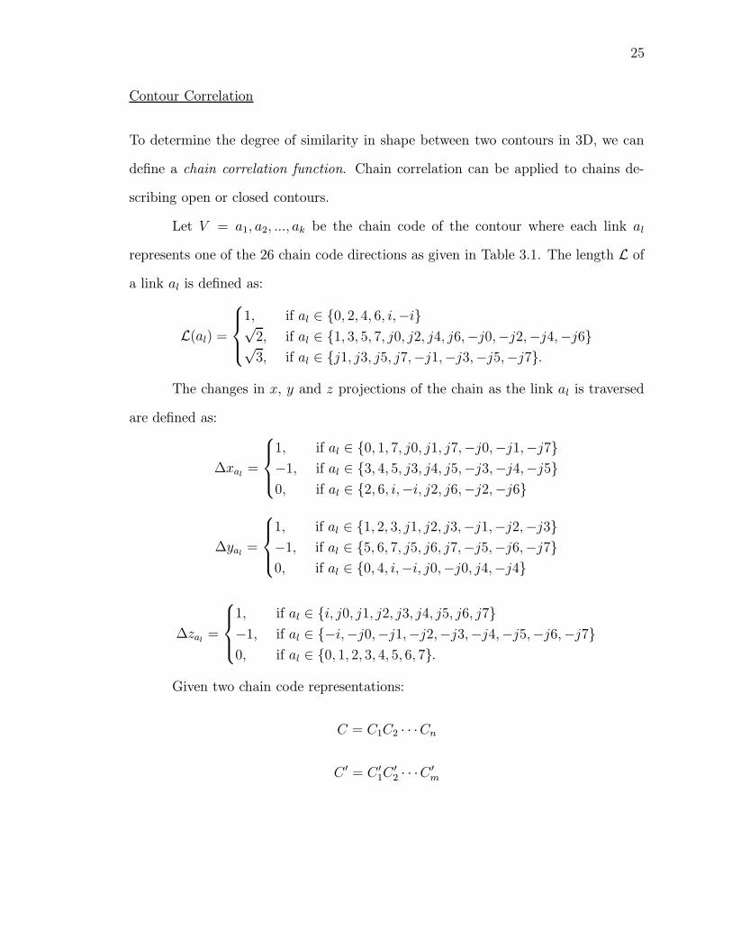
and

∆zl =

1, if al ∈ {i, j0, j1, j2, j3, j4, j5, j6, j7}−1, if al ∈ {−i,−j0,−j1,−j2,−j3,−j4,−j5,−j6,−j7}0, if al ∈ {0, 1, 2, 3, 4, 5, 6, 7}.

The projections on x, y and z of the first p links of the chain are respectively:

xp =

p∑

l=1

∆xl

yp =

p∑

l=1

∆yl

zp =

p∑

l=1

∆zl.

The Fourier series expansion for the x projection of the chain code of the complete

contour is given by:

x(t) = A0 +

∞∑

n=1

(Ancos2nπt

T+Bnsin

2nπt

T), t ∈ [0, T ], where

A0 =1

T

k∑

p=1

(∆xp2∆tp

(t2p − t2p−1) + βp(tp − tp−1))

where β1 = 0, βp =

p−1∑

j=1

∆xj −∆xp∆tp

p−1∑

j=1

∆tj

An =T

2n2π2

k∑

p=1

∆xp∆tp

[cos2nπtpT

− cos2nπtp−1

T]

Bn =T

2n2π2

k∑

p=1

∆xp∆tp

[sin2nπtpT

− sin2nπtp−1

T].

29

The Fourier series expansion for the y projection of the chain code of the

complete contour is given by:

y(t) = C0 +

∞∑

n=1

(Cncos2nπt

T+Dnsin

2nπt

T), t ∈ [0, T ], where

C0 =1

T

k∑

p=1

(∆yp2∆tp

(t2p − t2p−1) + δp(tp − tp−1))

where δ1 = 0, δp =

p−1∑

j=1

∆yj −∆yp∆tp

p−1∑

j=1

∆tj

Cn =T

2n2π2

k∑

p=1

∆yp∆tp

[cos2nπtpT

− cos2nπtp−1

T]

Dn =T

2n2π2

k∑

p=1

∆yp∆tp

[sin2nπtpT

− sin2nπtp−1

T].

The Fourier series expansion for the z projection of the chain code of the

complete contour is given by:

z(t) = E0 +∞∑

n=1

(Encos2nπt

T+ Fnsin

2nπt

T), t ∈ [0, T ], where

E0 =1

T

k∑

p=1

(∆zp2∆tp

(t2p − t2p−1) + γp(tp − tp−1))

where γ1 = 0, γp =

p−1∑

j=1

∆zj −∆zp∆tp

p−1∑

j=1

∆tj

En =T

2n2π2

k∑

p=1

∆zp∆tp

[cos2nπtpT

− cos2nπtp−1

T]

Fn =T

2n2π2

k∑

p=1

∆zp∆tp

[sin2nπtpT

− sin2nπtp−1

T].

Note that ∆tp =√

∆x2p +∆y2p +∆z2p . Thus, C(t) = (x(t), y(t), z(t)) repre-

sents the smooth form of the chain V = a1, a2, ..., ak.

The Matlab code which was used to implement the Fourier Descriptors for the

3D chain code is given in Appendix B.

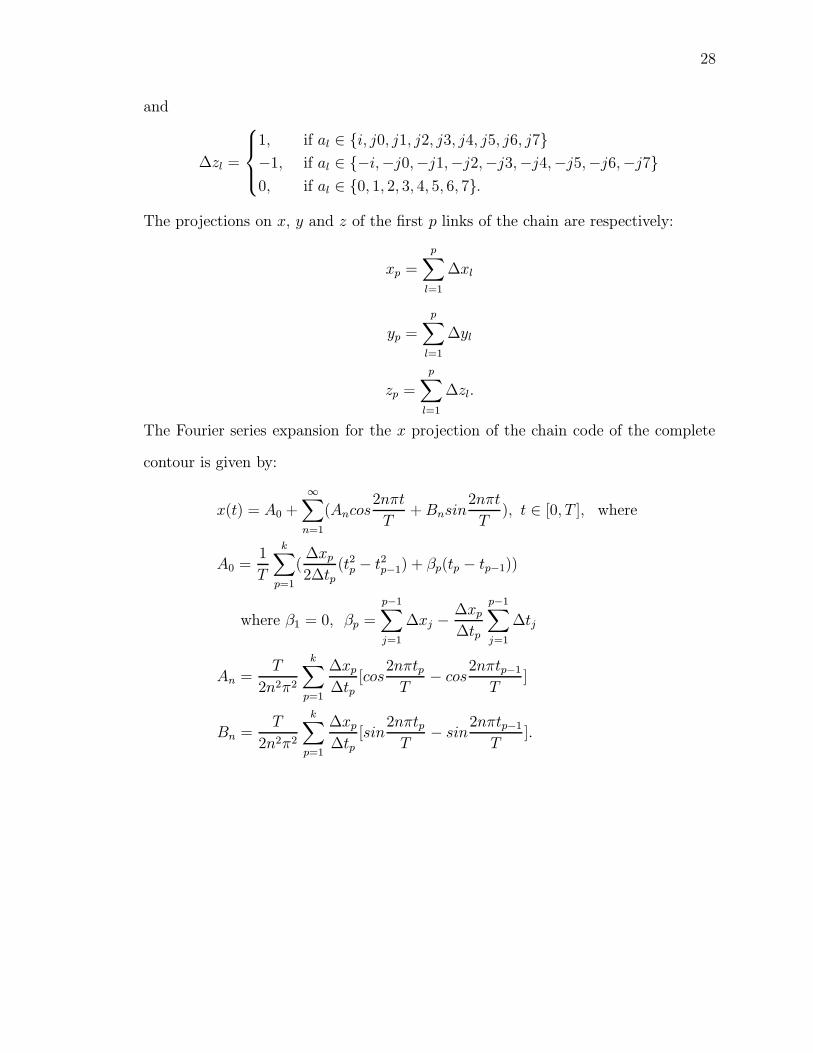
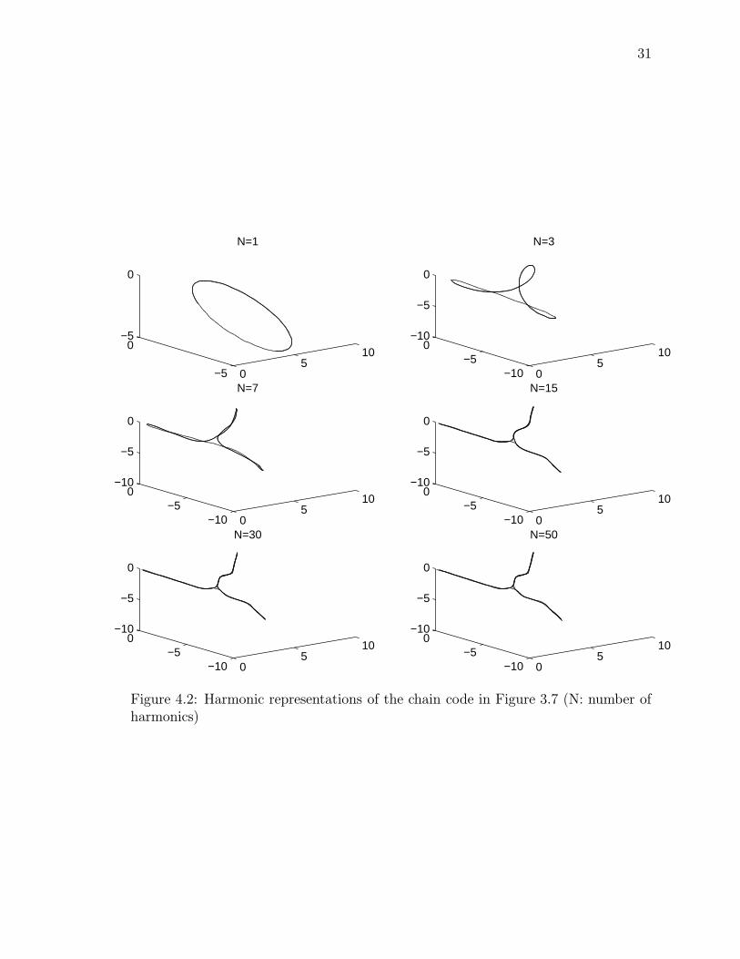
Figures 4.1 - 4.4 illustrate the result of applying the Fourier Descriptors de-

scribed above to the 3D chain code obtained using our algorithm in Chapter 3.

30

05

10

−5

0

5−1

0

1

N=1

−50

510

−5

0

5−1

0

1

N=5

−50

510

−5

0

5

10−1

01

N=15

0

5

10

−5

0

5

10−1

0

1

N=30

Figure 4.1: Harmonic representations of the chain code in Figure 3.6 (N: number ofharmonics)

31

05

10

−5

0−5

0

N=1

05

10

−10−5

0−10

−5

0

N=3

05

10

−10−5

0−10

−5

0

N=7

05

10

−10−5

0−10

−5

0

N=15

05

10

−10−5

0−10

−5

0

N=30

05

10

−10−5

0−10

−5

0

N=50


32

−50

5

−100

10−10

0

10

N=1

−50

5

−100

10−10

0

10

N=3

−50

510−10

0

10−10

0

10

N=5

−50510−100

10−10

0

10

N=10

−5 0 5 10−10

010

−10

−5

0

5

N=15

−5 0 5 10

−10

0

10−10

0

10

N=40


33

−50

5

−200

20−20

0

20

N=1

−50

510

−20−10

0−20

−10

0

N=3

−50

510

−20−10

0−20

−10

0

N=15

−50

510

−20−10

0−20

−10

0

N=25

−50

510

−20−10

0−20

−10

0

N=35

−50

510

−20−10

0−20

−10

0

N=70


34

4.2 Normalization of the Fourier coefficients for the 3D chain code

We describe an intuitive and mathematically pleasing way of normalizing the

Fourier coefficients obtained in the previous section. The resulting Fourier coefficients

are invariant with rotation, dilation, translation and the starting point on the contour

and lose no information about the shape of the contour.

Intuitively, normalizing a Fourier contour representation means placing the

first harmonic phasor of the Fourier series in a standard position. In our case, this

means translating the origin of the coordinate system to the center of the elliptic

first harmonic phasor and rotating the coordinate axes in such a way as to align the

X and Y axes with the semi-major and semi-minor axes of the ellipse respectively.

Thus, we obtain an ellipse on the XY-plane centered at the origin with the X and Y

axes corresponding to its semi-major and semi-minor axes respectively.

Consider the truncated Fourier series approximation to a closed contour:

x(t) = A0 +

N∑

n=1

Xn(t)

y(t) = C0 +N∑

n=1

Yn(t)

z(t) = E0 +

N∑

n=1

Zn(t)

where

Xn(t) = Ancos2nπt

T+Bnsin

2nπt

T

Yn(t) = Cncos2nπt

T+Dnsin

2nπt

T

Zn(t) = Encos2nπt

T+ Fnsin

2nπt

T, 1 ≤ n ≤ N, t ∈ [0, T ].

35

The first harmonic (N=1) of the Fourier series is given by:

x(t) = A0 + A1cos2πt

T+B1sin

2πt

T(4.1)

y(t) = C0 + C1cos2πt

T+D1sin

2πt

T(4.2)

z(t) = E0 + E1cos2πt

T+ F1sin

2πt

T. (4.3)

Notice that the first harmonic is an ellipse embedded in 3-space.

Subtracting the bias terms A0, C0, E0 from both sides of equations (4.1), (4.2),

(4.3) respectively is equivalent to translating the origin of the coordinate system to

the center of the elliptic first harmonic phasor.

Let

x1(t) = x(t)− A0

x2(t) = y(t)− C0

x3(t) = z(t)− E0.

Therefore,

x1(t) = A1cos2πt

T+B1sin

2πt

T

x2(t) = C1cos2πt

T+D1sin

2πt

T

x3(t) = E1cos2πt

T+ F1sin

2πt

T.

Notice that (x1(0), x2(0), x3(0)) is a vector in the direction of the positive semi-major

axis of the elliptic first harmonic phasor and (x1(T4), x2(

T4), x3(

T4)) is a vector in

the direction of the positive semi-minor axis of the elliptic first harmonic phasor.

Therefore,

~x′1 = (x1(0), x2(0), x3(0))

= (A1, C1, E1)

36

(t = T/4)

(t = 0)

O

(t = 3T/4)

(t = T/2)

X

Y

Z

U

W

V

Figure 4.5: The elliptic first harmonic phasor centered at the origin; X,Y,Z are theoriginal axes of the coordinate system; U,V,W are the axes in the new coordinatesystem

~x′2 = (x1(T

4), x2(

T

4), x3(

T

4))

= (B1, D1, F1).

Let ~x′3 ⊥ ~x′1 and ~x′

3 ⊥ ~x′2. From the property of cross product of two vectors and the

right hand rule, we know that

~x′3 = ~x′1 × ~x′2

Therefore,

~x′3 = (C1F1 − E1D1, B1E1 − A1F1, A1D1 −B1C1).

We know that ~e1 = (1, 0, 0), ~e2 = (0, 1, 0), ~e3 = (0, 0, 1) form a standard basis of R3.

It is easily verified that ~x′1, ~x′

2, ~x′

3 also form a basis of R3. Using elementary linear

algebra, the following transformation matrix or change of coordinate matrix can be

constructed:

A1 B1 C1F1 − E1D1

C1 D1 B1E1 − A1F1

E1 F1 A1D1 − B1C1

.

The above transformation matrix is used to rotate the X, Y, Z coordinate axes coun-

37

terclockwise into the U, V, W axes as shown in Figure 4.5. Let A∗

n, B∗

n, C∗

n, D∗

n, E∗

n

and F ∗

n denote the normalized Fourier coefficients for the 3D chain code. The com-

bined effects of an axial rotation and a displacement of the starting point on the

coefficients An, Bn, Cn, Dn, En and Fn of the original starting point are expressed in

matrix notation as follows:

A1 B1 C1F1 − E1D1

C1 D1 B1E1 − A1F1

E1 F1 A1D1 − B1C1

Ancos2nπtT

+Bnsin2nπtT

Cncos2nπtT

+Dnsin2nπtT

Encos2nπtT

+ Fnsin2nπtT

=

A∗

ncos2nπtT

+B∗

nsin2nπtT

C∗

ncos2nπtT

+D∗

nsin2nπtT

E∗

ncos2nπtT

+ F ∗

nsin2nπtT.

Therefore,

A∗

n = A1An +B1Cn + (C1F1 − E1D1)En

B∗

n = A1Bn +B1Dn + (C1F1 − E1D1)Fn

C∗

n = C1An +D1Cn + (B1E1 − A1F1)En

D∗

n = C1Bn +D1Dn + (B1E1 − A1F1)Fn

E∗

n = E1An + F1Cn + (A1D1 − B1C1)En

F ∗

n = E1Bn + F1Dn + (A1D1 − B1C1)Fn.

Notice that E∗

1 = F ∗

1 = 0. The contour classification can be made independent of size

by dividing each of the coefficients by the magnitude of the semi-major axis which is

(A21 + C2

1 + E21)

1

2 , and independent of translation by ignoring the bias terms A0, C0,

and E0.

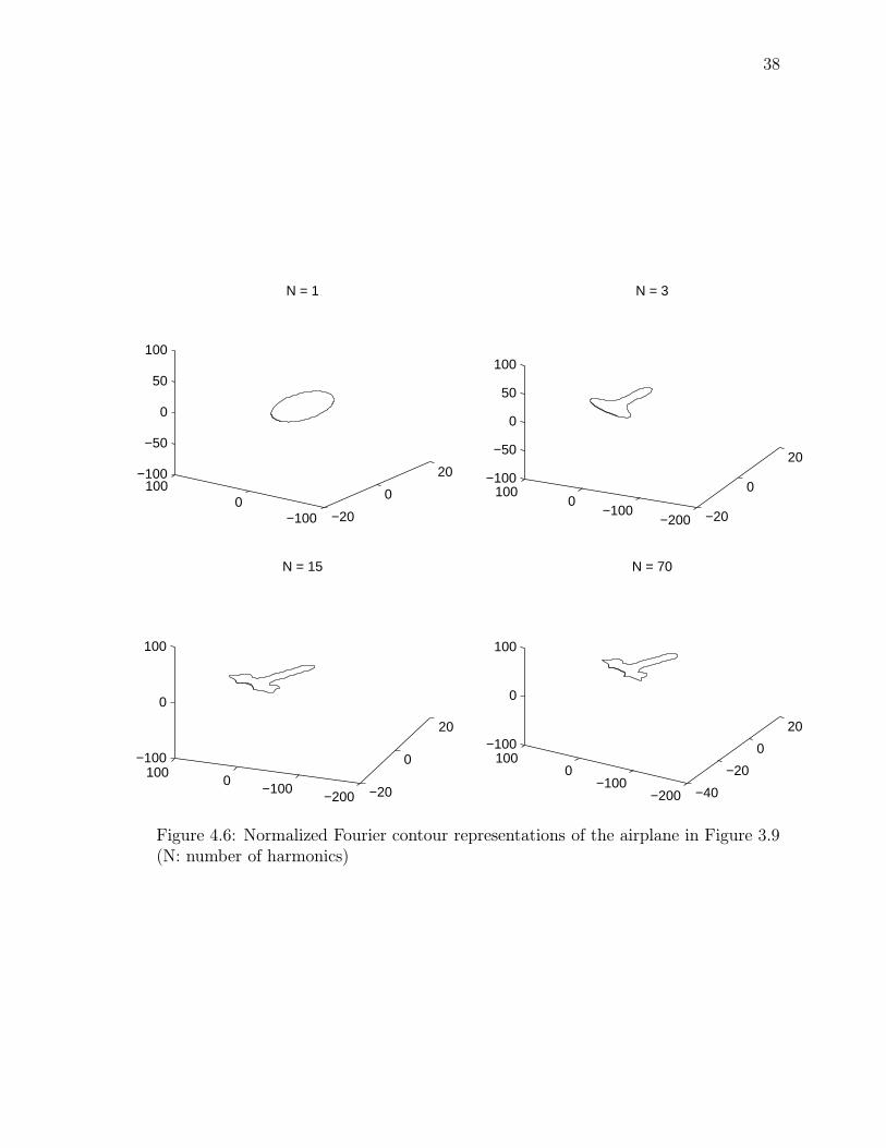
Figure 4.6 illustrates the normalized Fourier contour representation of the

airplane depicted in Figure 3.9.

38

−20

0

20

−1000

100−100

−50

0

50

100

N = 1

−20

0

20

−200−100

0100

−100

−50

0

50

100

N = 3

−20

0

20

−200−100

0100

−100

0

100

N = 15

−40

−20

0

20

−200−100

0100

−100

0

100

N = 70

Figure 4.6: Normalized Fourier contour representations of the airplane in Figure 3.9(N: number of harmonics)

CHAPTER 5CONCLUSIONS AND FUTURE WORK

We have described a simple and efficient scheme for encoding digitized 1-

dimensional curves in 3D. Using this scheme, we developed an algorithm for accu-

rately encoding any digitized 1-dimensional curve embedded in 3-space. Elementary

manipulations for the 3D chain code have been suggested.

Additionally, we developed Fourier Descriptors for the 3D chain code in order

to reconstruct the curve. We presented an intuitive and mathematically pleasing

technique for normalizing the Fourier coefficients of the 3D chain code. The resulting

Fourier Descriptors are invariant with rotation, dilation, translation and starting

point of the contour and lose no information about the shape of the contour. The

normalized Fourier Descriptors have potential applications in template matching and

pattern recognition problems.

Future work will involve finding a mathematically pleasing way of rotating

any arbitrary curve in 3D by simply using its chain code. So far, we know which

directions of the chain code should map to what directions when we rotate the curve

in terms of angles of ±90◦ or ±45◦ about any given axis, but we have not been able

to notice any pattern yet. Rotation in terms of arbitrary angles is a more challenging

problem.

Our encoding algorithm and the method of Fourier Descriptors are yet to

be tested on real images. Future work might involve application of the technique

for normalizing the Fourier coefficients of the 3D chain code to pattern recognition

problems. Hopefully, the work found in this thesis will lead to new techniques in the

area of pattern recognition.

39

APPENDIX AIMPLEMENTATION OF THE 3D CHAIN CODE

The following is the code in C which implements the chain code for an arbitrary

1-dimensional curve in 3D:

/********** IMPLEMENTATION OF THE 3D CHAIN CODE **********/

# include <stdio.h>

# include <stdlib.h>

# include <math.h>

/* CONSTANT DECLARATIONS */

# define num_points 100

# define xdim 25

# define ydim 25

# define zdim 25

# define TRUE 1

# define FALSE 0

typedef int BOOL;

/* GLOBAL VARIABLES */

int image[xdim][ydim][zdim];

int info[num_points][4];

int num_visited = -1;

int start_x = 0, start_y = 0, start_z = 0;

FILE *outfile;

/* FUNCTION DECLARATIONS */

/* checks to see if the point exists in the visited list */

BOOL exists_VL();

40

41

/* returns the 1st position of the point in the visited list */

int exists_VL_position();

BOOL visited();

/* checks if the coordinate of the point is out of range or not */

int range();

/* finds the inverse of a given direction */

int inverse_dir();

/* checks to see if a point of interest exists in the/

/* specified direction */

BOOL check();

BOOL check_dir();

/* finds the first point of interest in the image */

void Find_first();

/* MAIN METHOD: finds all points of interest starting */

/* from the firstpoint */

void Find_next();

/* writes the chain code to a file */

void write_image();

/*****************************************************************/

/* checks if point(x,y,z) occurs in the list of visited points */

BOOL exists_VL(int x, int y, int z)

{

BOOL exists = FALSE;

int i;

for (i = 0; i < num_points; i++)

42

{

if ((info[i][0] == x) && (info[i][1] == y) && (info[i][2] == z))

{ exists = TRUE;

break;

}

}

return exists;

}

/* returns the position of point(x,y,z) in the visited list */

int exists_VL_position(int x, int y, int z)

{

int i, pos;

for (i = 0; i < num_points; i++)

{

if ((info[i][0] == x) && (info[i][1] == y) && (info[i][2] == z))

{ pos = i;

break;

}

}

return pos;

}

/* checks if a point in a given direction from point(x,y,z) */

/* has been visited */

BOOL visited( int dir, int x, int y, int z)

{

43

BOOL flag = FALSE;

switch(dir) {

case 0: flag = exists_VL(x,y+1,z);

break;

case 1: flag = exists_VL(x-1,y+1,z);

break;

case 2: flag = exists_VL(x-1,y,z);

break;

case 3: flag = exists_VL(x-1,y-1,z);

break;

case 4: flag = exists_VL(x,y-1,z);

break;

case 5: flag = exists_VL(x+1,y-1,z);

break;

case 6: flag = exists_VL(x+1,y,z);

break;

case 7: flag = exists_VL(x+1,y+1,z);

break;

case 8: flag = exists_VL(x,y,z+1);

break;

case 9: flag = exists_VL(x,y,z-1);

break;

case 10: flag = exists_VL(x,y+1,z+1);

break;

case 11: flag = exists_VL(x-1,y+1,z+1);

break;

case 12: flag = exists_VL(x-1,y,z+1);

44

break;

case 13: flag = exists_VL(x-1,y-1,z+1);

break;

case 14: flag = exists_VL(x,y-1,z+1);

break;

case 15: flag = exists_VL(x+1,y-1,z+1);

break;

case 16: flag = exists_VL(x+1,y,z+1);

break;

case 17: flag = exists_VL(x+1,y+1,z+1);

break;

case 18: flag = exists_VL(x,y+1,z-1);

break;

case 19: flag = exists_VL(x-1,y+1,z-1);

break;

case 20: flag = exists_VL(x-1,y,z-1);

break;

case 21: flag = exists_VL(x-1,y-1,z-1);

break;

case 22: flag = exists_VL(x,y-1,z-1);

break;

case 23: flag = exists_VL(x+1,y-1,z-1);

break;

case 24: flag = exists_VL(x+1,y,z-1);

break;

case 25: flag = exists_VL(x+1,y+1,z-1);

break;

45

}

return flag;

}

/* checks whether point(m,n,p) is a legal pixel coordinate */

int range (int n, int m, int p)

{

if (n < 0 || n >= xdim) return 0;

if (m < 0 || m >= ydim) return 0;

if (p < 0 || p >= zdim) return 0;

return 1;

}

/* finds the inverse of a given direction */

int inverse_dir(int dir)

{

int inv;

switch(dir) {

case 0: inv = 4; break;









46


















}

return inv;

}

BOOL check (int x, int y, int z)

{

BOOL flag = FALSE;

if (range(x,y,z))

if (image[x][y][z] == 0)

47

flag =TRUE;

return flag;

}

/* checks whether a point(x,y,z) has a neighbor in a */

/* particular direction */

BOOL check_dir (int dir, int x, int y, int z)

{

BOOL flag = FALSE;

switch(dir) {

case 0: flag = check(x,y+1,z);

break;

case 1: flag = check(x-1,y+1,z);

break;

case 2: flag = check(x-1,y,z);

break;

case 3: flag = check(x-1,y-1,z);

break;

case 4: flag = check(x,y-1,z);

break;

case 5: flag = check(x+1,y-1,z);

break;

case 6: flag = check(x+1,y,z);

break;

case 7: flag = check(x+1,y+1,z);

break;

48

case 8: flag = check(x,y,z+1);

break;

case 9: flag = check(x,y,z-1);

break;

case 10: flag = check(x,y+1,z+1);

break;

case 11: flag = check(x-1,y+1,z+1);

break;

case 12: flag = check(x-1,y,z+1);

break;

case 13: flag = check(x-1,y-1,z+1);

break;

case 14: flag = check(x,y-1,z+1);

break;

case 15: flag = check(x+1,y-1,z+1);

break;

case 16: flag = check(x+1,y,z+1);

break;

case 17: flag = check(x+1,y+1,z+1);

break;

case 18: flag = check(x,y+1,z-1);

break;

case 19: flag = check(x-1,y+1,z-1);

break;

case 20: flag = check(x-1,y,z-1);

break;

case 21: flag = check(x-1,y-1,z-1);

49

break;

case 22: flag = check(x,y-1,z-1);

break;

case 23: flag = check(x+1,y-1,z-1);

break;

case 24: flag = check(x+1,y,z-1);

break;

case 25: flag = check(x+1,y+1,z-1);

break;

default: printf("Illegal code");

break;

}

return flag;

}

/* finds the first point by searching in column major order */

/* for each fixed z */

void Find_first()

{

int i,j,k;

for (k = zdim-1; k >= 0; k--)

for (j = 0; j < ydim; j++)

for (i = 0; i < xdim; i++)

{

if (image[i][j][k] == 0)

{

50

num_visited++;

goto loop_done;

}

}

loop_done: printf("Starting point: (%d, %d, %d) \n", i, j, k);

/* ASSUMPTION: chain code direction for starting point = -1 */

/* The starting point is not part of the list of visited points */

/* since one needs to come back to it to get a closed curve */

start_x = i;

start_y = j;

start_z = k;

Find_next();

}

/* finds the all pixels of interest starting with the first point

void Find_next()

{

int x,y,z,d,lastdir, prev_pos;

BOOL pt_found = TRUE;

x = start_x;

y = start_y;

z = start_z;

lastdir = -1;

for (;;) {

if (check_dir(1,x,y,z))

if ( !(visited(1,x,y,z)) )

51

{

num_visited++;

x = x-1;

y = y+1;

lastdir = 1; break;

}



{

num_visited++;

y = y+1;

lastdir = 0; break;

}



{

num_visited++;

x = x+1;

y = y+1;

lastdir = 7; break;

}



{

num_visited++;

x = x+1;

lastdir = 6; break;

52

}



{

num_visited++;

z = z-1;

lastdir = 9; break;

}



{

num_visited++;

z = z-1;

y = y+1;

lastdir = 18; break;

}



{

num_visited++;

x = x+1;

y = y+1;

z = z-1;


}



53

{

num_visited++;

x = x+1;

z = z-1;


}



{

num_visited++;

x = x+1;

y = y-1;

z = z-1;


}



{

num_visited++;

z = z-1;

y = y-1;


}



{

num_visited++;

54

x = x-1;

y = y-1;

z = z-1;


}



{

num_visited++;

x = x-1;

z = z-1;


}



{

num_visited++;

x = x-1;

y = y+1;

z = z-1;


}

} // end for

info[num_visited][0] = x;

info[num_visited][1] = y;

info[num_visited][2] = z;

55

info[num_visited][3] = lastdir;

for(;;) {

if (lastdir != inverse_dir(8))


if (!(visited(8,x,y,z)) )

{

num_visited++;

z = z+1;

lastdir = 8; break;

}




{

num_visited++;

y = y-1;

z = z+1;


}




{

num_visited++;

x = x-1;

y = y-1;

z = z+1;

56


}




{

num_visited++;

x = x-1;

z = z+1;


}




{

num_visited++;

x = x-1;

y = y+1;

z = z+1;


}




{

num_visited++;

57

y = y+1;

z = z+1;


}




{

num_visited++;

x = x+1;

y = y+1;

z = z+1;


}




{

num_visited++;

x = x+1;

z = z+1;


}




{

58

num_visited++;

x = x+1;

y = y-1;

z = z+1;


}




{

num_visited++;

y = y-1;

lastdir = 4; break;

}




{

num_visited++;

x = x-1;

y = y-1;

lastdir = 3; break;

}




{

59

num_visited++;

x = x-1;

lastdir = 2; break;

}




{

num_visited++;

x = x-1;

y = y+1;

lastdir = 1; break;

}




{

num_visited++;

y = y+1;

lastdir = 0; break;

}




{

num_visited++;

x = x+1;

60

y = y+1;

lastdir = 7; break;

}




{

num_visited++;

x = x+1;

lastdir = 6; break;

}




{

num_visited++;

x = x+1;

y = y-1;

lastdir = 5; break;

}




{

num_visited++;

z = z-1;

lastdir = 9; break;

61

}




{

num_visited++;

y = y-1;

z = z-1;


}




{

num_visited++;

x = x-1;

y = y-1;

z = z-1;


}




{

num_visited++;

x = x-1;

z = z-1;

62


}




{

num_visited++;

x = x-1;

y = y+1;

z = z-1;


}




{

num_visited++;

y = y+1;

z = z-1;


}




{

num_visited++;

x = x+1;

63

y = y+1;

z = z-1;


}




{

num_visited++;

x = x+1;

z = z-1;


}




{

num_visited++;

x = x+1;

y = y-1;

z = z-1;


}

} // end for




64


/* Search for all other points starting from the third point. */

/* This is necessary to make sure not to search along the */

/* direction from the second point to the starting point. */

do {

for (;;) {



{

num_visited++;

z = z+1;

lastdir = 8; break;

}



{

num_visited++;

y = y-1;

z = z+1;


}



{

num_visited++;

x = x-1;

65

y = y-1;

z = z+1;


}



{

num_visited++;

x = x-1;

z = z+1;


}



{

num_visited++;

x = x-1;

y = y+1;

z = z+1;


}



{

num_visited++;

y = y+1;

z = z+1;

66


}



{

num_visited++;

x = x+1;

y = y+1;

z = z+1;


}



{

num_visited++;

x = x+1;

z = z+1;


}



{

num_visited++;

x = x+1;

y = y-1;

z = z+1;


67

}



{

num_visited++;

y = y-1;

lastdir = 4; break;

}



{

num_visited++;

x = x-1;

y = y-1;

lastdir = 3; break;

}



{

num_visited++;

x = x-1;

lastdir = 2; break;

}



{

num_visited++;

68

x = x-1;

y = y+1;

lastdir = 1; break;

}



{

num_visited++;

y = y+1;

lastdir = 0; break;

}



{

num_visited++;

x = x+1;

y = y+1;

lastdir = 7; break;

}



{

num_visited++;

x = x+1;

lastdir = 6; break;

}


69


{

num_visited++;

x = x+1;

y = y-1;

lastdir = 5; break;

}



{

num_visited++;

z = z-1;

lastdir = 9; break;

}



{

num_visited++;

y = y-1;

z = z-1;


}



{

num_visited++;

x = x-1;

70

y = y-1;

z = z-1;


}



{

num_visited++;

x = x-1;

z = z-1;


}



{

num_visited++;

x = x-1;

y = y+1;

z = z-1;


}



{

num_visited++;

y = y+1;

z = z-1;

71


}



{

num_visited++;

x = x+1;

y = y+1;

z = z-1;


}



{

num_visited++;

x = x+1;

z = z-1;


}



{

num_visited++;

x = x+1;

y = y-1;

z = z-1;


72

}

pt_found = FALSE; break;

} // end for

if (pt_found)

{





}

else {

prev_pos = exists_VL_position(x,y,z);

d = info[prev_pos][3];

lastdir = inverse_dir(d);

pt_found = TRUE;

num_visited++;

switch(lastdir) {

case 0: y = y+1; break;

case 1: x = x-1;

y = y+1; break;

case 2: x = x-1; break;

case 3: x = x-1;

y = y-1; break;

case 4: y = y-1; break;

case 5: x = x+1;

y = y-1; break;

case 6: x = x+1; break;

73

case 7: x = x+1;

y = y+1; break;

case 8: z = z+1; break;

case 9: z = z-1; break;

case 10: y = y+1;

z = z+1; break;

case 11: x = x+1;

y = y+1;

z = z+1; break;

case 12: x = x-1;

z = z+1; break;

case 13: x = x-1;

y = y-1;

z = z+1; break;

case 14: y = y-1;

z = z+1; break;

case 15: x = x+1;

y = y-1;

z = z+1; break;

case 16: x = x+1;

z = z+1; break;

case 17: x = x+1;

y = y+1;

z = z+1; break;

case 18: y = y+1;

z = z-1; break;

case 19: x = x-1;

74

y = y+1;

z = z-1; break;

case 20: x = x-1;

z = z-1; break;

case 21: x = x-1;

y = y-1;

z = z-1; break;

case 22: y = y-1;

z = z-1; break;

case 23: x = x+1;

y = y-1;

z = z-1; break;

case 24: x = x+1;

z = z-1; break;

case 25: x = x+1;

y = y+1;

z = z-1; break;

}





if (exists_VL(x,y,z))

{

prev_pos = exists_VL_position(x,y,z);

lastdir = info[prev_pos][3];

}

75

}

} while ( (x!=start_x) || (y!=start_y) || (z!=start_z) );

}

/* generates a vase in 3D */

void test_image()

{

int i,j,k;

for (k = zdim-1; k >= 0; k--)

for (j = 0; j < ydim; j++)

for (i = 0; i < xdim; i++)

image[i][j][k] = 1;

image[1][3][10] = 0;

image[1][4][10] = 0;

image[1][5][10] = 0;

image[1][6][10] = 0;

image[1][7][10] = 0;

image[2][4][9] = 0;

image[2][6][9] = 0;

image[3][4][8] = 0;

image[3][6][8] = 0;

image[4][3][7] = 0;

image[4][7][7] = 0;

image[5][2][6] = 0;

image[5][8][6] = 0;

image[6][2][5] = 0;

76

image[6][8][5] = 0;

image[7][3][4] = 0;

image[7][4][4] = 0;

image[7][5][4] = 0;

image[7][6][4] = 0;

image[7][7][4] = 0;

}

/* write the chain code to a file */

void write_image(char* imagefile)

{

FILE *ofile;

int i;

if ( !(ofile=fopen(imagefile,"w")))

{

printf("Can’t open write file \n");

exit(1);

}

for (i=1; i<= num_visited; i++)

{

fprintf(ofile, "%d", info[i][3]);

fprintf(ofile," ");

}

fclose(ofile);

}

77

main()

{

// test image

test_image();

Find_first();

/* write the chaincode to the file ’chaincode’ */

outfile = fopen("chaincode","w");

write_image("chaincode");

printf("Number of points in chain code: %d \n", num_visited);

return 0;

}

APPENDIX BIMPLEMENTATION OF THE FOURIER DESCRIPTORS

The following is the code in Matlab that implements the Fourier Descriptors

for the 3D chain code obtained using the encoding process described in Chapter 3:

%%% IMPLEMENTATION OF THE FOURIER DESCRIPTORS

%%% -------------------------------------

function f = FD(num)

% num: number of harmonics

% file ’chaincode’ contains the chaincode of the 1-D curve

% code: vector representing the chain code

% k: length of the chain code

% T: basic period of the chain code

code = load(’chaincode’);

k = length(code);

T = time_cum(code,k);

t = 0:pi/5:10*pi;

size_t = length(t);

A_zero=0; C_zero=0; E_zero=0;

tic;

for p = 1:k

A_zero = A_zero + (delta_x(code(p))/(2*delta_t(code(p))))

* (sqr(time_cum(code,p))-sqr(time_cum(code,p-1)

+ Beta(code,p) * (time_cum(code,p)

78

79

- time_cum(code,p-1));

C_zero = C_zero + (delta_y(code(p))/(2*delta_t(code(p))))


+ Delta(code,p) * (time_cum(code,p)


E_zero = E_zero + (delta_z(code(p))/(2*delta_t(code(p))))


+ Gamma(code,p) * (time_cum(code,p)


end

A_zero = (1/T)*A_zero;

C_zero = (1/T)*C_zero;

E_zero = (1/T)*E_zero;

x_t = zeros(1,size_t);

y_t = zeros(1,size_t);

z_t = zeros(1,size_t);

for n = 1:num

A = (T/(2*sqr(n)*sqr(pi))) * An(code,n,T);

B = (T/(2*sqr(n)*sqr(pi))) * Bn(code,n,T);

C = (T/(2*sqr(n)*sqr(pi))) * Cn(code,n,T);

D = (T/(2*sqr(n)*sqr(pi))) * Dn(code,n,T);

E = (T/(2*sqr(n)*sqr(pi))) * En(code,n,T);

F = (T/(2*sqr(n)*sqr(pi))) * Fn(code,n,T);

x_t = x_t + A*cos(2*n*pi*t/T) + B*sin(2*n*pi*t/T);

y_t = y_t + C*cos(2*n*pi*t/T) + D*sin(2*n*pi*t/T);

80

z_t = z_t + E*cos(2*n*pi*t/T) + F*sin(2*n*pi*t/T);

end

x_t = A_zero + x_t;

y_t = C_zero + y_t;

z_t = E_zero + z_t;

toc;

figure(1), rotate3d on

%%%% (x_t, y_t, z_t) represents the smooth form of the chain

plot3(x_t,y_t,z_t)

f = T;

function a=sqr(x)

a=x*x;

% --- function to calculate the time needed to traverse link i

function a = time(i)

if ( (i==0) | (i==2) |(i==4) |(i==6) |(i==8) |(i==9) )

a = 1;

else if ( (i==11) | (i==13) |(i==15) |(i==17) |(i==19)

|(i==21)|(i==23)|(i==25))

a = sqrt(3);

else a = sqrt(2);

end

end

81

% --- function to calculate the time required to traverse ---

% --- first p links in the chain ---

function a = time_cum(code,p)

sum = 0;

for i = 1:p

sum = sum + time(code(i));

end

a = sum;

function a = delta_t(p)

a = sqrt( sqr(delta_x(p)) + sqr(delta_y(p)) +sqr(delta_z(p)) );

% --- function to calculate the change in x-projection as ---

% --- link i is traversed ---

function a = delta_x(i)

if ( (i==0) | (i==1) | (i==7) | (i==10) | (i==11) | (i==17)

| (i==18) | (i==19) | (i==25))

a = 1;

else if ( (i==3) | (i==4) | (i==5)| (i==13) | (i==14) | (i==15)

|(i==21) | (i==22) | (i==23) )

a = -1;

else a = 0;

end

end

% --- function to calculate the change in y-projection as ---


82

function a = delta_y(i)

if ( (i==1) | (i==2) | (i==3)| (i==11) | (i==12) | (i==13)

|(i==19) | (i==20) | (i==21))

a = 1;

else if ( (i==5) | (i==6) | (i==7)| (i==15) | (i==16)

| (i==17)|(i==23) | (i==24) | (i==25))

a = -1;

else a = 0;

end

end

% --- function to calculate the change in z-projection as ---


function a = delta_z(i)

if ( (i>=0) & (i<=7) )

a = 0;

else if ( (i==8) | ((i>=10) & (i<=17)) )

a = 1;

else a = -1;

end

end

% --- functions to calculate the Fourier coefficients An, Bn, ---

% --- Cn, Dn, En and Fn corresponding to the nth harmonics ---

function a = An(code,n,T)

k = length(code);

sum = 0;

83

for p = 1:k

sum = sum + (delta_x(code(p))/delta_t(code(p)))

* (cos(2*n*pi*time_cum(code,p)/T)

- cos(2*n*pi*time_cum(code,p-1)/T) );

end

a = sum;

function a = Bn(code,n,T)

k = length(code);

sum = 0;

for p = 1:k

sum = sum + (delta_x(code(p))/delta_t(code(p)))

* (sin(2*n*pi*time_cum(code,p)/T)

- sin(2*n*pi*time_cum(code,p-1)/T) );

end

a = sum;

function a = Cn(code,n,T)

k = length(code);

sum = 0;

for p = 1:k

sum = sum + (delta_y(code(p))/delta_t(code(p)))



end

a = sum;

84

function a = Dn(code,n,T)

k = length(code);

sum = 0;

for p = 1:k

sum = sum + (delta_y(code(p))/delta_t(code(p)))



end

a = sum;

function a = En(code,n,T)

k = length(code);

sum = 0;

for p = 1:k

sum = sum + (delta_z(code(p))/delta_t(code(p)))



end

a = sum;

function a = Fn(code,n,T)

k = length(code);

sum = 0;

for p = 1:k

sum = sum + (delta_z(code(p))/delta_t(code(p)))



85

end

a = sum;

% functions to calculate the DC components in the Fourier series

function a = Beta(code,p)

sum1 = 0;

if(p==1)

a = 0;

else

for i =1:(p-1)

sum1 = sum1 + delta_x(code(i));

end

sum2 = time_cum(code,p-1);

a = sum1 - (delta_x(code(p))/delta_t(code(p))) * sum2;

end

function a = Delta(code,p)

sum1 = 0;

if(p==1)

a = 0;

else

for i =1:(p-1)

sum1 = sum1 + delta_y(code(i));

end


a = sum1 - (delta_y(code(p))/delta_t(code(p))) * sum2;

end

86

function a = Gamma(code,p)

sum1 = 0;

if(p==1)

a = 0;

else

for i =1:(p-1)

sum1 = sum1 + delta_z(code(i));

end


a = sum1 - (delta_z(code(p))/delta_t(code(p))) * sum2;

end

REFERENCES

[1] B. Bascle and R. Deriche, Stereo matching, reconstruction and refinement of3D curves using deformable contours, Proceedings of the Fourth InternationalConference on Computer Vision, Berlin, Germany, May 1991, pp.421–430.

[2] A. Blumenkrans, Two-dimensional object recognition using a two-dimensionalpolar transform, Pattern Recognition, 24, 1991, pp.879–890.

[3] E. Bribiesca, A chain code for representing 3D curves, Pattern Recognition, 33,2000, pp.755-765.

[4] E. Bribiesca and A. Guzman, How to describe pure form and how to measuredifferences in shapes using shape number, Pattern Recognition, 12, 1980, pp.101-112.

[5] W.K. Chow and J.K. Aggarwal, Computer analysis of dynamic scenes containingcurvilinear figures, IEEE Trans. Comput., 26, 1977, pp.179–185.

[6] F. Cohen and J. Wang, Part I: Modeling image curves using invariant 3Dobject curve models - a path to 3D recognition and shape estimation from imagecontours, IEEE Trans. Pattern Anal. Mach. Intell. (PAMI), 16(2), 1994, pp.1–12.

[7] L.S. Davis, Shape matching using relaxation techniques, IEEE Trans. PatternAnal. Mach. Intell. (PAMI), 1, 1979, pp.60–72.

[8] L.S. Davis Hierarchical relaxation for shape analysis, Proc. Pattern Recognitionand Image Processing Conference, Chicago, 1978, pp.275–279.

[9] H. Freeman, A techinique for the classification and recognition of geometric pat-terns, Proc. 3rd Intl. Congress on Cybernetics, Namur, Belgium,, 1961, pp.348–368.

[10] H. Freeman, On the encoding of arbitrary geometric configurations, IRE Trans.on Electron. Comput., EC-10, 1961, pp.260–268.

[11] H. Freeman, Techniques for the digital computer analysis of chain-encoded arbi-trary plane curves, Proc. Natl. Elect. Conf., 17, 1961, pp.421–432.

[12] H. Freeman, Computer processing of line drawing images, ACM ComputingSurveys, 6, 1974, pp.57-97.

[13] G.H. Granlund, Fourier preprocessing for hand print character recognition, IEEETrans. Comput., C-21, 1972, pp.195–201.

[14] A. Guzman, Fourier preprocessing for hand print character recognition, MCCTechnical Report Number: ACA-254-87, Austin, TX, 1987.

87

88

[15] A. Jonas and N. Kiryati, Digital representation schemes for 3D curves, Patternrecognition, 30, 1997, pp.1803–1814.

[16] C.E. Kim, Three-dimensional digital segments, Pattern Anal. Mach. Intell.(PAMI), 5, 1983, pp.231–234.

[17] R. Klette, The m-dimensional grid point space, Comput. Vision Graphics ImageProcess., 30, 1985, pp.1–12.

[18] F.P. Kuhl, Classification and recognition of hand-printed characters, IEEEInternation Convention Record, Pt. 4, 1963, pp.75–93.

[19] F.P. Kuhl, J. Weber, D. O’Connor and C.R. Giardina, Fourier series approx-imation of chain-encoded contours, Proc. Electro-Optics Laser 80 Conferenceand Exposition, Boston, MA, 1980, pp.317–331.

[20] F.P. Kuhl and C.R. Giardina, Elliptic Fourier features of closed contours, Tech-nical Report, ARRADCOM, Dover, NJ, 1981.

[21] M.D. Levine Vision in Man and Machine, McGraw-Hill, New York, 1985.

[22] W.N. Martin and J.K. Aggarwal, Computer analysis of dynamic scenes contain-ing curvilinear figures, Pattern Recognition, 11, 1979, pp.169–178.

[23] J.W. McKee and J.K. Aggarwal, Finding the edges of the surfaces of three-dimensional curved objects by computer, Pattern Recognition, 7, 1975, pp.25–52.

[24] J.W. McKee and J.K. Aggarwal, Computer recognition of partial views of curvedobjects, IEEE Trans. Comput., C-26, 1977, pp.790–800.

[25] R.D. Merrill, Representation of contours and regions for efficient computersearch, Commun. ACM, 16, 1969, pp.534–549.

[26] E. Persoon and K.S. Fu,, Shape discrimination using Fourier descriptors, IEEETrans. Syst., Man., Cybern., SMC-7, 1977, pp.170–179.

[27] A. Rosenfeld, Connectivity in digital pictures, J. ass. Comp. Mach., 26, 1970,pp.146–160.

[28] A. Rosenfeld, Digital straight line segments, IEEE Trans. Comput., 23, 1974,pp.1264-1269.

[29] A. Rosenfeld, Digital topology, Amer. Math. Monthly, 86, 1979, pp.621-630.

[30] A. Rosenfeld, Three-dimensional digital topology, Inform. and Control, 50, 1981,pp.119–127.

[31] G.S. Sidhu and R.T. Boute, Property encoding: applications to binary pictureencoding and boundary following, IEEE trans. Comput., C-21, 1972, pp.1206–1216.

[32] I. Stojmenovic and R. Tosic, Digitization schemes and the recognition of digitalstraight lines, hyperplanes and flats in arbitrary dimensions, Contemp. Math.,119, 1991, pp.197-212.

[33] R. Vaillant and O. Faugeras, Using extremal boundaries for 3D object modeling,IEEE Trans. PAMI, 14(2), 1992, pp.157–173.

89

[34] T.P. Wallace and O.R. Mitchell, Analysis of three-dimensional movement usingFourier descriptors, IEEE Trans. PAMI, 2(6), 1980, pp.583–588.

[35] T.P. Wallace and P.A. Wintz, An efficient three-dimensional aircraft recognitionalgorithm using normalized Fourier descriptors, Computer Graphics and ImageProcessing, 13(2), 1980, pp.99–126.

[36] C.S. Zhao, Epipolar parametrization for reconstructing 3D rigid curve, PatternRecognition, 30, 1997, pp.1817-1827.

BIOGRAPHICAL SKETCH

Paromita Bose was born in Calcutta, India, on September 14, 1976. She grad-

uated with a Bachelor of Science (with honors) in Mathematics from the University

of Delhi, India in July 1997.

In August 1997, she came to the United States to pursue graduate degrees in

Mathematics and Computer and Information Science and Engineering concurrently.

Her love of mathematics made her continue towards a graduate degree in that area.

However, her fascination since childhood and interest in Computer Science motivated

her to pursue the Computer Science graduate degree.

In December 1999, she graduated with a Master of Science in Mathemat-

ics (with specialization in Applied Mathematics) from the University of Florida,

Gainesville, FL, under the direction of Dr. Yunmei Chen. Her thesis was on Partial

Differential Equation (PDE) based image processing. She graduates with her Mas-

ter of Science in Computer and Information Science and Engineering in December

2000. Her interests include pattern recognition, image processing, computer vision

and neural networks. Someday she hopes to pursue a Ph.D. in Computer Science.

90

Documents

THE ENCODING AND FOURIER DESCRIPTORS OF ...ufdcimages.uflib.ufl.edu/UF/00/10/07/51/00001/Thesis_ETD.pdfTHE ENCODING AND FOURIER DESCRIPTORS OF ARBITRARY CURVES IN 3-DIMENSIONAL SPACE