Embed Size (px)
Citation preview

The Effects of Wakes on Separating Boundary Layers in Low Pressure Turbines
Rory Douglas Stieger
Peterhouse
A dissertation submitted for the degree of doctor of Philosophy
Cambridge University Engineering Department
February 2002
ii
Abstract An experimental investigation into wake-induced transition in
separating boundary layers was conducted. Measurements were made on a flat plate
with an imposed pressure distribution and on a 2D cascade of LP turbine blades. The
unsteady effects of wakes were simulated in both facilities by wake generators
consisting of cylindrical bars traversed across the inlet flow.
Single component LDA measurements were made on the flat plate with a
technique developed to measure the ensemble averaged Reynolds stresses by making
measurements at multiple probe orientations. These measurements allowed the
boundary layer dissipation to be determined thus providing experimental proof of the
loss reducing mechanisms arising from wake induced unsteady transition processes.
Evidence of a deterministic natural transition processes by Tollmein-Schlichting
waves was also identified in the boundary layer between wake passing events. The
frequency of these waves matches that of the most amplified disturbance in a Falkner-
Skan profile of the same displacement thickness.
The convection of a turbulent wake through a LP turbine cascade was
measured using 2D LDA. The resolution of these measurements is unprecedented and
the measurements will provide a database for future CFD validation. The wake
turbulence was found to be anisotropic. The production of turbulent kinetic energy
was calculated from the 2D LDA measurements and found to increase the levels of
turbulent kinetic energy of the wake fluid at approximately mid chord.
Unsteady blade surface pressures were measured on the suction surface of the
T106 LP turbine cascade. Large amplitude pressure oscillations were observed to
arise as the wake passed over the region that was occupied by a separation bubble in
steady flow conditions. The source of these pressure oscillations was identified to be
vortices embedded in the suction surface boundary layer.

iii
Preface The work reported in this thesis was performed at the Whittle Laboratory,
Cambridge University Engineering Department between October 1999 and January
2002. Except where specifically stated to the contrary, this dissertation is my own
work and includes nothing that is the result of collaboration. No part of this
dissertation has been submitted to any other academic establishment.
This thesis comprises eight chapters and four appendices, which total
approximately 51 000 words and 80 figures.
Rory Stieger

iv
Acknowledgement Although the preface says that this work is all my own it is very clear to me
that it was in fact made possible by a great number of people.
G. D. J Smith and J.P. Bindon were instrumental in instilling in me a
fascination with turbomachinery. I am indebted to them not only for this but also their
efforts to pave the way for my further study. AECI Ltd was also generous in releasing
me from contractual obligations thereby allowing me to follow a dream.
I am indebted for the financial support provided by a Peterhouse Research
Studentship, the ORS trust, and the EPSRC.
The staff of the Whittle Laboratory workshops have always produced work of
unrivalled calibre. I am particularly indebted to the nimble fingers and endless
patience of T. Chandler, while I am also particularly grateful for the assistance of J.
Saunders, B. Taylor and K. Bryant.
Colleagues of the Whittle Lab have not only provided a fun working
environment but have been a valuable source of assistance, encouragement and
friendship.
It has become quite plain to me that any person gaining further sight or greater
understanding has done so by standing on the shoulders of a giant. Prof. H. Hodson
has been such a giant in his supervision of this work. I am most grateful for his
guidance and the opportunities he has afforded me.
It is right that the ultimate acknowledgement be to my parents, for their
unending love and support.
v
Nomenclature Symbols ϕ analysing wavelet ω angular frequency α anisotropy; probe angle Γ circulation ρ density β Falkner-Skan pressure gradient parameter φ flow coefficient φ=Vx/Ub ν kinematic viscosity ν=µ/ρ
θ momentum thickness dyU
u
U
u
y∫= ∞∞
−=
δ
θ0
1
λ Pohlhausen pressure gradient parameter dx
dU∞=νδλ
2
ψ principal stress direction µ viscosity
Ω vorticity y
U
x
V
∂∂−
∂∂=Ω
λθ Thwaites pressure gradient parameter dx
dU∞=νθλθ
2
δ* displacement thickness dyU
u
y∫= ∞
−=
δ
δ0
* 1
δ’ Blackwelder Parameter ∫=
+=98
0
2221
298
, )''(1
δ
δy
dyvuU
τ time constant τ0 bar passing period τconv convective time scale δj wavelet scale resolution τvisc viscous time scale τyx shear stress in boundary layer C chord CD non-turb non-turbulent component of dissipation coefficient CD turb turbulent component of dissipation coefficient CD dissipation coefficient Cp Coefficient of pressure Cp=(P01-P)/(P01-P2s) d diameter DTKE dissipation of TKE f frequency fr reduced frequency fr=fC/V2is H12 shape factor H12=δ*/θ M measured component of velocity vector P pressure
Nomenclature
vi
PTKE production of TKE
Q velocity vector magnitude 22 VUQ += r radius Reθ momentum thickness Reynolds number Reδ* displacement thickness Reynolds number Re2C Reynolds number based on isentropic exit velocity and blade chord s surface distance; wavelet scale s0 suction surface length sb bar pitch sc cascade pitch Stθ Strouhal number based on momentum thickness Stθ=fθ/U T temperature t time TKE Turbulent kinetic energy tr residence time of LDA sample Tu turbulence intensity U∞ freestream velocity U*,V* non-dimensional velocity; U*=U/V2is, V*=V/V 2is
2'u , 2'v Reynolds normal stresses
''vu Reynolds shear stress Ub bar speed or blade speed V velocity vθ radial velocity Vx axial velocity x distance x*, y* non-dimensional distance x*=x/C, y*=y/C Subscripts 0 total 1 inlet 2 exit ψ aligned to principal stress direction f fluid is isentropic p perturbation; particle s static t transition Superscripts * non-dimensional • complex conjugate Other X time average of X <X> ensemble-average of X W(X) continuous wavelet transform of X X Fourier transform of X

vii
Contents
Abstract ........................................................................................................................ ii
Preface......................................................................................................................... iii
Acknowledgement ...................................................................................................... iv
Nomenclature................................................................................................................v
Contents...................................................................................................................... vii
Chapter 1: Introduction ..............................................................................................1
1.1 Research motivation.........................................................................................1
1.2 Unsteady aerodynamics in LP turbines .........................................................1
1.3 Thesis overview.................................................................................................4
1.4 Figures ...............................................................................................................6
Chapter 2: Literature Review .....................................................................................9
2.1 Introduction ......................................................................................................9
2.2 Boundary layer transition ...............................................................................9 2.2.1 Natural transition in steady flow ................................................................9 2.2.2 Intermittency methods for transition........................................................11 2.2.3 Transition onset correlations ....................................................................12
2.2.3.1 Transition onset ....................................................................................13 2.2.3.2 Transition length ..................................................................................15
Spot formation rate correlations.......................................................................15 Minimum transition length correlations...........................................................18
2.2.4 Direct simulation of bypass transition......................................................19 2.2.5 Comments on the presented correlations .................................................20
2.3 Unsteady transition in turbomachines .........................................................22 2.3.1 Introduction ..............................................................................................22 2.3.2 Unsteady wake induced transition in attached boundary layers ..............24 2.3.3 Direct simulation of unsteady transition ..................................................28 2.3.4 Comments on unsteady transition ............................................................28
2.4 Separation bubbles.........................................................................................29 2.4.1 Structure of a separation bubble...............................................................29 2.4.2 Previous research on separation bubbles..................................................30 2.4.3 Transition in separation bubbles ..............................................................30

Contents
viii
2.4.4 Unsteady effects on separation bubbles ...................................................34 2.4.5 Unsteady transition with separated boundary layers................................36 2.4.6 Comments on separation bubble literature...............................................36
2.5 Concluding remarks.......................................................................................37
2.6 Figures .............................................................................................................38
Chapter 3: Experimental Methods ...........................................................................44
3.1 Introduction ....................................................................................................44
3.2 Experimental facilities ...................................................................................44 3.2.1 Wind tunnel ..............................................................................................44 3.2.2 Bar passing flat plate ................................................................................44 3.2.3 Bar passing cascade..................................................................................45 3.2.4 T106 low pressure turbine cascade ..........................................................46 3.2.5 Artificial disturbance generator................................................................47
3.3 Instrumentation..............................................................................................47 3.3.1 Data logging .............................................................................................47 3.3.2 Pressure measurements ............................................................................48
3.3.2.1 Conventional blade static pressure measurements ...............................48 3.3.2.2 Unsteady blade surface pressure measurements ..................................48
3.3.3 Hot wire measurements............................................................................50 3.3.4 Laser Doppler anemometry......................................................................51 3.3.5 Digital particle image velocimetry...........................................................54
3.4 Figures .............................................................................................................57
Chapter 4: The interaction of wakes with the separating boundary layer on a flat plate .............................................................................................................................65
4.1 Introduction ....................................................................................................65
4.2 Experimental details ......................................................................................66 4.2.1 Matching flat plate and cascade boundary layers.....................................66 4.2.2 Modelling the unsteady flow conditions for the flat plate .......................66 4.2.3 Details of boundary layer measurements .................................................68 4.2.4 Validation of the flat plate pressure distribution......................................69 4.2.5 Validation of flat plate boundary layer ....................................................69
4.3 Ensemble averaged measurements for wake boundary layer interaction70 4.3.1 Unsteady freestream disturbance environment ........................................70 4.3.2 Response of the boundary layer through a wake passing cycle ...............71 4.3.3 Space Time description of boundary layer state ......................................72
4.4 Transition between wake passing .................................................................74 4.4.1 Introduction ..............................................................................................74 4.4.2 Evidence of Natural transition phenomena in ensemble average measurements ...........................................................................................................75

Contents
ix
4.4.3 Simple correlation for wave frequency ....................................................76 4.4.4 Implications for transition modelling between wake passing ..................77
4.5 Boundary Layer Dissipation .........................................................................78 4.5.1 Introduction ..............................................................................................78 4.5.2 Calculation of Dissipation........................................................................78 4.5.3 Space time description of boundary layer dissipation..............................79 4.5.4 Observed mechanisms of viscous dissipation ..........................................80 4.5.5 Comparison of measured and expected levels of dissipation...................82
4.6 Conclusion from Flat Plate measurements ..................................................83
4.7 Figures .............................................................................................................85
Chapter 5: Measurement of turbulent wake convection through an axial turbine cascade.........................................................................................................................99
5.1 Introduction ....................................................................................................99
5.2 Measurement details ....................................................................................100
5.3 The kinematics of wake convection through a turbine cascade...............101 5.3.1 Mean flow ..............................................................................................101 5.3.2 Perturbation flow....................................................................................101
5.3.2.1 Kinematic wake convection ...............................................................102 5.3.2.2 Negative jet ........................................................................................102 5.3.2.3 Vorticity .............................................................................................103
5.4 Convection of wake turbulence through a turbine cascade .....................104 5.4.1 Turbulent kinetic energy ........................................................................104 5.4.2 Anisotropy..............................................................................................106
5.5 Ensemble average wavelet analysis of LDA data ......................................107 5.5.1 Ensemble average wavelet description of Reynolds stresses.................108 5.5.2 Ensemble average wavelet description of turbulent kinetic energy.......111
5.6 Conclusions ...................................................................................................113
5.7 Figures ...........................................................................................................115
Chapter 6: Unsteady pressures measured on the suction surface of the T106 LP Turbine cascade........................................................................................................128
6.1 Introduction ..................................................................................................128
6.2 Time mean surface pressure distribution ..................................................129
6.3 Ensemble average suction surface pressures.............................................130 6.3.1 Unsteady surface pressures ....................................................................131 6.3.2 The effect of bar passing frequency .......................................................133 6.3.3 The effect of a boundary layer trip.........................................................134

Contents
x
6.3.4 The effect of Reynolds number on pressure fluctuations.......................134 6.3.5 The interaction of a wave packet with the separating boundary layer ...135
6.4 The formation of coherent structures in a separating shear layer ..........136
6.5 Visualisation of the instantaneous flow field using PIV ...........................138
6.6 The source of surface pressure fluctuations ..............................................139
6.7 Description of Mechanism...........................................................................141 6.7.1 Hot wire measurements..........................................................................141 6.7.2 A schematic view of the origin of pressure fluctuations........................141
6.8 Conclusions ...................................................................................................143
6.9 Figures ...........................................................................................................145
Chapter 7: Boundary layer measurements on the T106 LP turbine cascade.....161
7.1 Introduction ..................................................................................................161
7.2 Details of 2D LDA boundary layer measurements ...................................161
7.3 Wake induced transition schematic for LP turbines ................................162 7.3.1 A traditional schematic of wake induced transition ...............................162 7.3.2 Schematic of wake-induced transition with inflexional boundary layer profiles 163
7.4 An S-T view of the measured boundary layer ...........................................164 7.4.1 Boundary Layer Edge Velocity..............................................................165 7.4.2 TKE thickness ........................................................................................165 7.4.3 Integral Parameters.................................................................................167
7.5 Unsteady boundary layer development......................................................168 7.5.1 Boundary layer state before the interaction of the wake and inflexional profiles 169 7.5.2 Interaction of wake and inflexional boundary layer...............................170 7.5.3 Boundary layer after wake interaction ...................................................171 7.5.4 Calmed boundary layer ..........................................................................172
7.6 Kelvin-Helmholtz breakdown of the shear layer ......................................173
7.7 Conclusions ...................................................................................................173
7.8 Figures ...........................................................................................................175
Chapter 8: Conclusions and recommendations for future work .........................189
8.1 Conclusions ...................................................................................................189 8.1.1 Flat Plate.................................................................................................189 8.1.2 T106 LP turbine cascade........................................................................190

Contents
xi
8.2 Recommendations for future work.............................................................190
References .................................................................................................................193
II.1 Introduction ..................................................................................................202
II.2 Derivation......................................................................................................202
II.3 Evaluation of Technique..............................................................................204
II.4 Discussion......................................................................................................205
II.5 Conclusions ...................................................................................................206
II.6 Figures ...........................................................................................................207
III.1 Introduction ..................................................................................................210
III.2 Wavelet Algorithm for LDA data...............................................................210
IV.1 Calculation of derivatives ............................................................................213
IV.2 Calculation of turbulent dissipation ...........................................................213


1
Chapter 1: Introduction
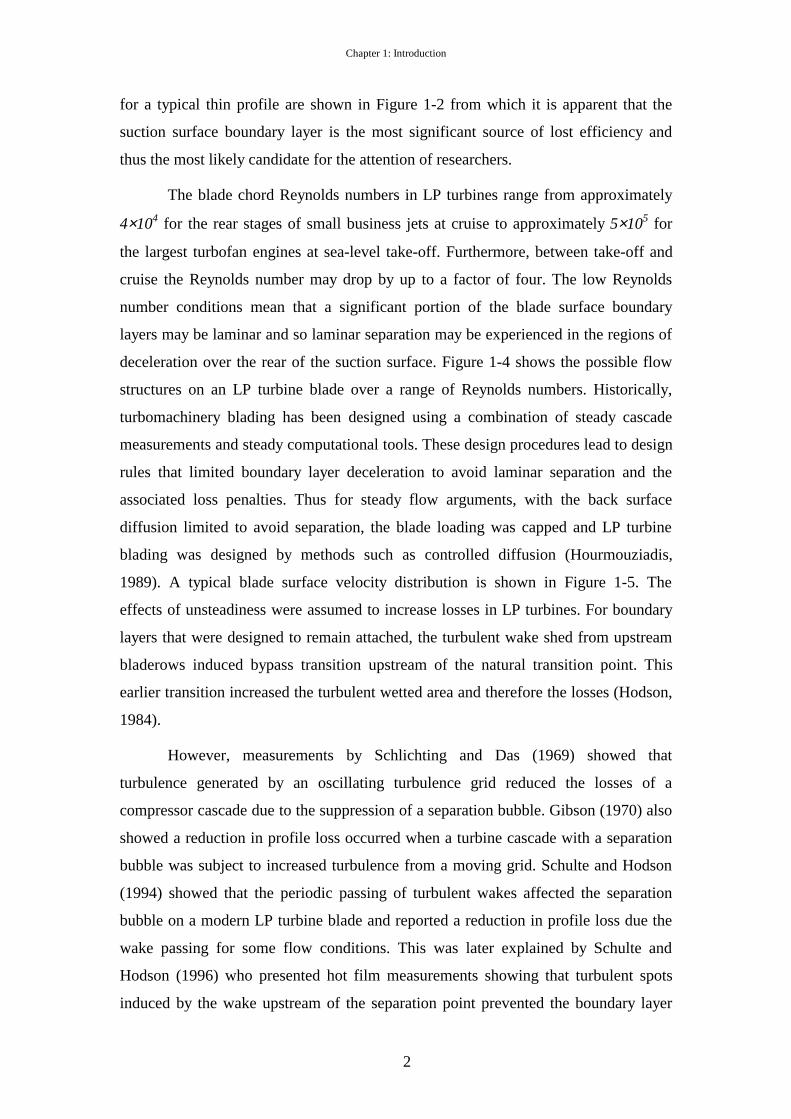
1.1 Research motivation Gas turbines are suited to aero-engine applications due to a combination of
high power-to-weight ratio and high efficiency. Most of the thrust of modern high by-
pass ratio turbofan engines, such as that shown in Figure 1-1, comes from the fan,
which is driven by the low-pressure (LP) turbine.
Due to the high power requirements of the fan, the LP turbine consists of
several stages. Furthermore, the low rotational speed imposed by the fan leads to large
diameters. As a result, the LP turbine is heavy, up to a third of the total engine weight,
and expensive to manufacture.
The efficiency of the gas turbine engine is critically dependant on the LP
turbine efficiency. Typically, a 1% increase in the polytropic efficiency of the LP
turbine will improve the engine’s fuel consumption by 0.5% (Hodson, 1998). For this
reason much effort has been devoted to developing highly efficient LP turbines and
current aero-engines have LP turbines efficiencies of 90% - 93%. In the last 50 years
of development, the LP turbine efficiency has only improved by about 13% and
further increases in efficiency are increasingly difficult to achieve.
The primary concern for aero-engine operators is the total cost of engine
ownership, which considers not only the capital cost but also the operating costs that
are influenced by efficiency, weight and reliability. Recent development (Cobley at al,
1997) has shown that the blade count of an LP turbine can be reduced by 20% without
significant efficiency penalties by capitalising on unsteady transition phenomena
found on LP turbine blade boundary layers. Reducing the number of blades in this
way reduces both the weight and manufacturing cost of the engine. This provides a
substantial reduction to the total cost of engine ownership.
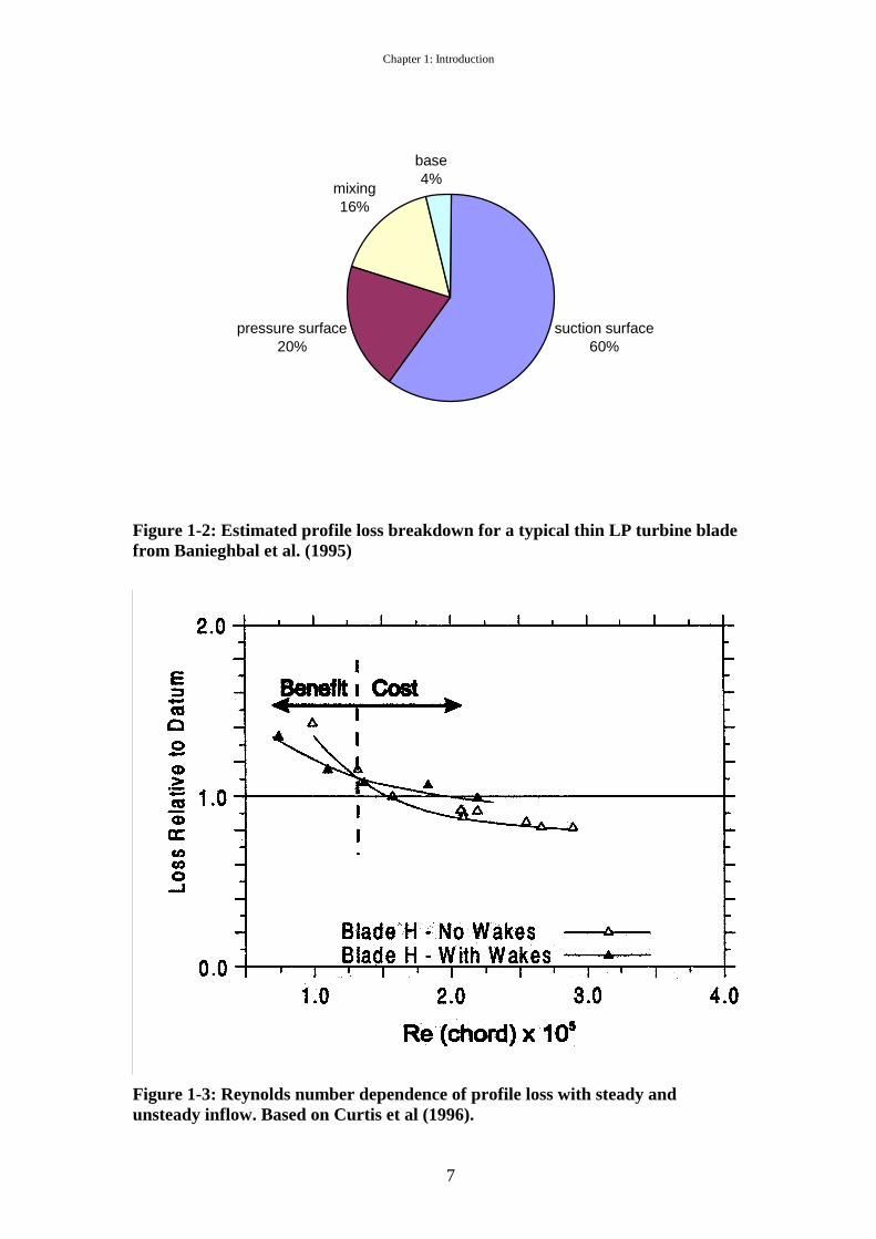
1.2 Unsteady aerodynamics in LP turbines LP turbine blades have a large aspect ratio, typically in the range 3-7:1 and as
a result secondary flows occupy only a small fraction of the blade span. The profile
loss thus contributes most significantly to the lost efficiency. The profile loss is made
up of contributions from the boundary layers of the suction and pressure surfaces,
mixing losses and base pressure losses. The relative magnitudes of these components
Chapter 1: Introduction
2
for a typical thin profile are shown in Figure 1-2 from which it is apparent that the
suction surface boundary layer is the most significant source of lost efficiency and
thus the most likely candidate for the attention of researchers.
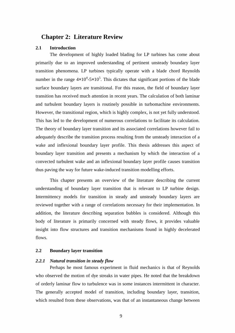
The blade chord Reynolds numbers in LP turbines range from approximately
4×10⁴ for the rear stages of small business jets at cruise to approximately 5×10⁵ for
the largest turbofan engines at sea-level take-off. Furthermore, between take-off and
cruise the Reynolds number may drop by up to a factor of four. The low Reynolds
number conditions mean that a significant portion of the blade surface boundary
layers may be laminar and so laminar separation may be experienced in the regions of
deceleration over the rear of the suction surface. Figure 1-4 shows the possible flow
structures on an LP turbine blade over a range of Reynolds numbers. Historically,
turbomachinery blading has been designed using a combination of steady cascade
measurements and steady computational tools. These design procedures lead to design
rules that limited boundary layer deceleration to avoid laminar separation and the
associated loss penalties. Thus for steady flow arguments, with the back surface
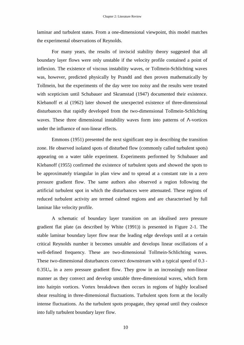
diffusion limited to avoid separation, the blade loading was capped and LP turbine
blading was designed by methods such as controlled diffusion (Hourmouziadis,
1989). A typical blade surface velocity distribution is shown in Figure 1-5. The
effects of unsteadiness were assumed to increase losses in LP turbines. For boundary
layers that were designed to remain attached, the turbulent wake shed from upstream
bladerows induced bypass transition upstream of the natural transition point. This
earlier transition increased the turbulent wetted area and therefore the losses (Hodson,
1984).
However, measurements by Schlichting and Das (1969) showed that
turbulence generated by an oscillating turbulence grid reduced the losses of a
compressor cascade due to the suppression of a separation bubble. Gibson (1970) also
showed a reduction in profile loss occurred when a turbine cascade with a separation
bubble was subject to increased turbulence from a moving grid. Schulte and Hodson
(1994) showed that the periodic passing of turbulent wakes affected the separation
bubble on a modern LP turbine blade and reported a reduction in profile loss due the
wake passing for some flow conditions. This was later explained by Schulte and
Hodson (1996) who presented hot film measurements showing that turbulent spots
induced by the wake upstream of the separation point prevented the boundary layer
Chapter 1: Introduction
3
from separating. The calmed regions that follow the turbulent spots were also shown
to be responsible for suppressing separation due to their elevated shear and full
velocity profiles.
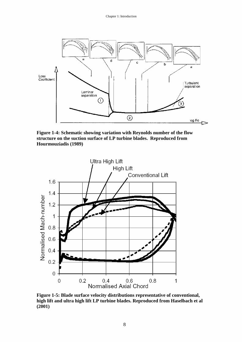
Loss reductions are thus intimately linked to the relative portions of the blade
surface covered by laminar, turbulent, calmed and separated flow. These phenomena
are all Reynolds number dependant and as a result, the profile loss depends on the
Reynolds number. This is true for steady and unsteady flows as shown in Figure 1-3.
For this profile, it is apparent that below a critical Reynolds number the unsteady flow
has lower losses than the steady flow. As the Reynolds number decreases, the steady
flow losses rise due to the increased extent of separation. In the wake passing case,
the separation is periodically suppressed by the turbulent and calmed flow. In the time
average, the losses generated during the turbulent and calmed periods contribute less
than the steady separation and this leads to loss reduction.
Armed with this improved understanding of unsteady transition, the traditional
steady flow design rules that limited boundary layer diffusion were challenged. A new
generation of blade profiles was designed based on the extensive experimental work
of Curtis et al (1996) and Howell et al (2000). These ‘high lift’ LP turbine blade
profiles, of which a typical velocity distribution is shown in Figure 1-5, were reported
to reduce the blade count of the LP turbine by 20% (Cobley et al, 1997) thus
achieving the ultimate goal of reducing the cost of ownership by simultaneously
reducing weight and manufacturing costs while providing little efficiency penalty. A
further reduction in blade count of 11% was reported by Haselbach et al. (2001) with
the advent of ‘Ultra High Lift’ blades. The resulting blade surface velocity
distribution shown in Figure 1-5 can be seen to have still higher levels of diffusion on
the rear of the suction surface. However, such increases in blade loading were only
possible when accompanied by the extensive experimental validation of Brunner et al
(2000), Howell et al (2000) and Howell et al (2001).
Despite drastic reductions in blade count and significant savings to
manufacturers and operators, the fundamental transition mechanisms involved in
reducing losses are not fully understood and unsteady design tools are in the early
stages of development, primarily due to inadequacies in understanding of the unsteady
transition phenomena associated with highly decelerated and separated boundary
layers.
Chapter 1: Introduction
4
1.3 Thesis overview The work reported in this thesis seeks primarily to identify the mechanism by
which boundary layer transition occurs when the wake shed from an upstream
bladerow interacts with the highly decelerated boundary layer on the suction surface
of a highly loaded LP turbine blade. In particular, the interaction between the
turbulent wake and the unsteady separation bubble that re-establishes between wake
passing events is investigated.
Chapter 2 presents a review of the literature pertaining to boundary layer
transition and separation bubbles. Details of the experimental methods used in the
course of research are presented in Chapter 3 together with a description of the
experimental facilities employed.
A fundamental study, conducted on a flat plate with a pressure gradient
matched to that measured on the T106 LP turbine cascade, is presented in Chapter 4.
Evidence of deterministic natural transition phenomena between wake passing events
was found and the boundary layer dissipation was measured thereby providing
experimental proof of the loss reducing mechanism exploited by modern high lift LP
turbine blade designs.
Chapter 5 presents detailed measurements of the wake convection through the
T106 LP turbine cascade. The use of 2D LDA and a very fine measurement grid
provides unprecedented detail and resolution of the turbulent quantities.
The unsteady blade surface boundary layer on the T106 LP turbine cascade is
then investigated. Chapter 6 presents measurements of the unsteady blade surface
pressures that reveal large amplitude pressure oscillations that arise as the wake
passes over the location of the steady separation bubble. The source of the pressure
oscillations is identified to be vortices embedded in the boundary layer. Chapter 7
presents evidence of these vortices in ensemble averaged 2D LDA boundary layer
measurements. The vortices are identified to form in the separated shear layer of the
separating boundary layer by an inviscid Kelvin-Helmholtz breakdown that is
triggered by wake passing. Finally, conclusions and recommendations for further
work are presented in Chapter 8.
Co-ordinates of the T106 profile investigated are presented in Appendix I,
while a novel technique for the measurement of 2D Reynolds stresses with 1D LDA is

Chapter 1: Introduction
5
presented in Appendix II. An algorithm for the wavelet transform of randomly
sampled data is presented in Appendix III while Appendix IV presents details of the
calculation of derivatives and the calculation of the dissipation of turbulent kinetic
energy used in the thesis.
Chapter 1: Introduction
6
1.4 Figures
Figure 1-1: Cutaway section of a modern high bypass civil aircraft engine. Detail shows the LP turbine. Reproduced from Howell (1999)
Chapter 1: Introduction
7
suction surface60%
pressure surface20%
mixing16%
base4%
Figure 1-2: Estimated profile loss breakdown for a typical thin LP turbine blade from Banieghbal et al. (1995)
Figure 1-3: Reynolds number dependence of profile loss with steady and unsteady inflow. Based on Curtis et al (1996).
Chapter 1: Introduction
8
Figure 1-4: Schematic showing variation with Reynolds number of the flow structure on the suction surface of LP turbine blades. Reproduced from Hourmouziadis (1989)
Figure 1-5: Blade surface velocity distributions representative of conventional, high lift and ultra high lift LP turbine blades. Reproduced from Haselbach et al (2001)
9
Chapter 2: Literature Review
2.1 Introduction The development of highly loaded blading for LP turbines has come about
primarily due to an improved understanding of pertinent unsteady boundary layer
transition phenomena. LP turbines typically operate with a blade chord Reynolds
number in the range 4×10⁴-5×10⁵. This dictates that significant portions of the blade
surface boundary layers are transitional. For this reason, the field of boundary layer
transition has received much attention in recent years. The calculation of both laminar
and turbulent boundary layers is routinely possible in turbomachine environments.
However, the transitional region, which is highly complex, is not yet fully understood.
This has led to the development of numerous correlations to facilitate its calculation.
The theory of boundary layer transition and its associated correlations however fail to
adequately describe the transition process resulting from the unsteady interaction of a
wake and inflexional boundary layer profile. This thesis addresses this aspect of
boundary layer transition and presents a mechanism by which the interaction of a
convected turbulent wake and an inflexional boundary layer profile causes transition
thus paving the way for future wake-induced transition modelling efforts.
This chapter presents an overview of the literature describing the current
understanding of boundary layer transition that is relevant to LP turbine design.
Intermittency models for transition in steady and unsteady boundary layers are
reviewed together with a range of correlations necessary for their implementation. In
addition, the literature describing separation bubbles is considered. Although this
body of literature is primarily concerned with steady flows, it provides valuable
insight into flow structures and transition mechanisms found in highly decelerated
flows.
2.2 Boundary layer transition
2.2.1 Natural transition in steady flow Perhaps he most famous experiment in fluid mechanics is that of Reynolds
who observed the motion of dye streaks in water pipes. He noted that the breakdown
of orderly laminar flow to turbulence was in some instances intermittent in character.
The generally accepted model of transition, including boundary layer, transition,
which resulted from these observations, was that of an instantaneous change between
Chapter 2: Literature Review
10
laminar and turbulent states. From a one-dimensional viewpoint, this model matches
the experimental observations of Reynolds.
For many years, the results of inviscid stability theory suggested that all
boundary layer flows were only unstable if the velocity profile contained a point of
inflexion. The existence of viscous instability waves, or Tollmein-Schlichting waves
was, however, predicted physically by Prandtl and then proven mathematically by
Tollmein, but the experiments of the day were too noisy and the results were treated
with scepticism until Schubauer and Skramstad (1947) documented their existence.
Klebanoff et al (1962) later showed the unexpected existence of three-dimensional
disturbances that rapidly developed from the two-dimensional Tollmein-Schlichting
waves. These three dimensional instability waves form into patterns of Λ-vortices
under the influence of non-linear effects.
Emmons (1951) presented the next significant step in describing the transition
zone. He observed isolated spots of disturbed flow (commonly called turbulent spots)
appearing on a water table experiment. Experiments performed by Schubauer and
Klebanoff (1955) confirmed the existence of turbulent spots and showed the spots to
be approximately triangular in plan view and to spread at a constant rate in a zero
pressure gradient flow. The same authors also observed a region following the
artificial turbulent spot in which the disturbances were attenuated. These regions of
reduced turbulent activity are termed calmed regions and are characterised by full
laminar like velocity profile.
A schematic of boundary layer transition on an idealised zero pressure
gradient flat plate (as described by White (1991)) is presented in Figure 2-1. The
stable laminar boundary layer flow near the leading edge develops until at a certain
critical Reynolds number it becomes unstable and develops linear oscillations of a
well-defined frequency. These are two-dimensional Tollmein-Schlichting waves.
These two-dimensional disturbances convect downstream with a typical speed of 0.3 -
0.35U∞ in a zero pressure gradient flow. They grow in an increasingly non-linear
manner as they convect and develop unstable three-dimensional waves, which form
into hairpin vortices. Vortex breakdown then occurs in regions of highly localised
shear resulting in three-dimensional fluctuations. Turbulent spots form at the locally
intense fluctuations. As the turbulent spots propagate, they spread until they coalesce
into fully turbulent boundary layer flow.
Chapter 2: Literature Review
11
If the disturbance levels are high or the pressure gradient is strongly adverse a
bypass transition may occur. In such a case the process of formation, growth and
breakdown, of the instability waves occurs very rapidly or is bypassed entirely and
turbulent spots form immediately in the laminar boundary layer.
2.2.2 Intermittency methods for transition From his observations on a water table, Emmons (1951) was able to conclude
that transition occurs by the formation of turbulent spots within a laminar boundary
layer. The turbulent spots form randomly in time and space through a transition
region. Each spot grows as it propagates downstream until the spots coalesce into a
turbulent boundary layer. The process of transition is random in time and space and
can best be described by a probability function specifying the fraction of time that the
flow at a point in the transition zone is covered by turbulent flow. This fraction of
time that the flow is turbulent is known as the intermittency, γ, and has values ranging
from γ=0 for a laminar boundary layer to γ=1 for a fully turbulent boundary layer.
Based on his observations, Emmons developed a ‘Probability Transition Theory’ to
determine the intermittency distribution based on the rate of formation of turbulent
spots per unit area and knowledge of how the spots propagate in the flow.
With insufficient information at his disposal Emmons went on to determine
the chordwise intermittency distribution for a flat plate by assuming a constant
turbulent spot formation rate and a simple model for the spot propagation.
The data of Schubauer and Klebanoff (1955) highlighted the failing of
Emmons’ assumptions to correctly describe the transition zone. However, the
necessary agreement between experiment and theory was provided by Narasimha’s
(1957) concentrated breakdown hypothesis. Based on experimental observations that
spots formed only in a narrow band, Narasimha hypothesized that the spot production
rate could be represented by a Dirac delta function. Dhawan and Narasimha (1958)
showed that this hypothesis adequately predicted all the mean flow properties in the
transition zone.
Although the concentrated breakdown hypothesis provided the necessary
agreement between experiment and theory, no explanation for its success was
provided for almost 40 years. Schulte (1995) described how spot formation is
suppressed in the calmed region that follows a turbulent spot. The genesis of spots
Chapter 2: Literature Review
12
occurs at a particular location, but downstream of that location, spot formation is
suppressed due to the influence of existing spots and their calmed regions. Based on
this observation Schulte went on to describe a corrected spot production rate by
accounting for the effect of existing spots and calmed regions.
A more thorough development of the concepts proposed by Schulte (1995)
was given by Ramesh and Hodson (1999) who presented a closed form solution for
the corrected spot production rate in a zero pressure gradient flow. By approximating
the calmed region behind each spot by a rectangular shape, they showed excellent
agreement with the intermittency distribution of Narasimha. This provided an
important physical explanation of the success of the concentrated breakdown model.
Application of the model of Ramesh and Hodson (1999) showed excellent
agreement with that of Narasimha, where under adverse pressure gradients the spot
production is limited to a narrow band by both models. Under zero pressure gradient
flow, however, the spot production in the new model occurred over a wider range
with the resulting intermittency distribution being delayed. This offset is, however,
small compared to the transition zone length and could be accounted for by
modifications to the transition onset location. No comparison with experimental
results was presented.
The suppression of spot formation by existing turbulent spots was previously
documented by Johnson and Fashifar (1994) who conducted a series of measurements
in a transitional boundary layer on a zero pressure gradient flat plate. Using an
intermittency routine to distinguish between laminar and turbulent flow, they
proceeded to calculate statistics of the burst-length, gap-length and spacing between
turbulent events and found that new turbulent spots were not formed randomly but
were suppressed within a recovery period adjacent to existing turbulent spots.
2.2.3 Transition onset correlations Transition is known to be affected by a wide range of parameters including:
Reynolds number, Mach number, acoustic radiation, surface roughness, surface
temperature, surface curvature and flow history. However, the dominant parameters in
the turbomachinery environment are the streamwise pressure gradient and the free
stream turbulence and it is upon these two parameters that most correlations are
based.
Chapter 2: Literature Review
13
In order to apply the intermittency model in the transition zone one requires
knowledge of the spot production and propagation rates as well as the onset location
of transition. Current understanding of the transition process is, however, insufficient
to allow the prediction of the necessary parameters. This has necessitated the
development of correlations to determine transition onset, spot production rate and
transition length in terms of flow conditions at transition onset.
2.2.3.1 Transition onset Linear stability theory for laminar boundary layers indicates that transition is
predominantly brought about by the amplification of disturbances in the boundary
layer. At a critical displacement thickness Reynolds number, the boundary layer
becomes susceptible to disturbances that grow and lead to transition. This process is
however not fully understood and as a result experimental data and correlations must
be used to facilitate the prediction of transition. In the turbomachinery environment,
where disturbances abound from a range of sources, primarily turbulence, the use of
experimental data and correlations is vital for engineering calculations.
An extensive experimental study on transition in attached boundary layers
representative of turbomachinery environments was performed by Abu-Ghannam and
Shaw (1980). Based on a combination of published data and their own, they provided
a correlation for transition onset as a function of turbulence level and pressure
gradient. It was noted that the pressure gradient has a less significant effect on
transition onset at higher turbulence levels. Although Abu-Ghannam and Shaw noted
the importance of turbulent length scale, they found that it had little effect on
transition onset.
Mayle (1991) correlates transition onset with turbulence in zero pressure
gradient flows and arrives at an expression similar to that previously suggested by
Hourmouziadis (1989). He notes that Abu-Ghannam and Shaw’s correlation forced
data to fit at low turbulence and to level out at the minimum stability criteria. These
measures are seen as unnecessary in light of the influence of acoustic disturbances at
very low turbulence levels1. Although insufficient data was available for a reliable
1 The irrelevance of stability theory to by-pass transition is cited by Mayle as a reason to dismiss the need for the minimum limit imposed by Abu-Ghannam and Shaw. Walker (1993), however comments that stability theory and its governing parameters are applicable and relevant to estimating transition length.
Chapter 2: Literature Review
14
correlation, Mayle suggests the use of Taylor’s turbulence parameter2 to account for
the effect of turbulent length scale, using momentum thickness as a length parameter.
Based on the assumption that turbulence far outweighs the influence of pressure
gradient in gas turbine environments, Mayle (1991) proposes his zero pressure
gradient correlation for transition onset as sufficient for all conditions with turbulence
level above 3%.
In an attempt to add physical insight to the transition onset problem, Johnson
(1993) argued that the start of transition could be inferred from laminar fluctuations of
the near wall velocity that are induced by freestream turbulence. He argues that if the
near wall velocity drops below half the mean local velocity then the near wall flow
will stall and separate instantaneously, a mechanism that is consistent with the
formation of hairpin vortices known to precede breakdown. Johnson’s simplistic
argument was able to show that this condition corresponds to a local turbulence level
of 23%, which agrees with near wall measurements at the start of transition for a
range of freestream turbulence intensities and pressure gradients. A complementary
physical argument suggests that the local turbulence level is a measure of streamline
distortion and that the streamline distortion corresponding to a turbulence level of
23% is the maximum that can be tolerated prior to breakdown. By assuming a
Pohlhausen velocity profile, Johnson was able to produce a semi-empirical formula to
predict the start of transition as a function of pressure gradient and turbulence.
However, the results do not show a significant improvement over those of Abu-
Ghannam and Shaw (1980).
Mayle and Schulz (1997) present a separate analysis for calculating
fluctuations in the laminar boundary layer resulting from a turbulent freestream. Their
analysis, based on that of Lin (1957), derived an equation for the kinetic energy of
fluctuations in a laminar boundary layer. It was found that the only link between the
fluctuations in the freestream and the boundary layer was through the production of
laminar kinetic energy in the boundary layer by the work of imposed fluctuating
pressure forces in the freestream. After formulating models for the production and
dissipation of the laminar fluctuations, calculations were performed to predict
2 5
LTuTa
θ= where Ta is Taylor’s turbulence parameter, Tu is the turbulence intensity, θ the
momentum thickness and L the turbulence length scale.
Chapter 2: Literature Review
15
transition onset. Limited success was attributed to inadequacies in the models for
production, dissipation and the absence of a suitable universal onset criterion.
2.2.3.2 Transition length The transition length in turbomachinery flows has usually been determined by
one of two approaches, namely the minimum transition length concept introduced by
Walker (1989) or the spot formation rate concept of Narasimha (1985) 3. Both
approaches depend primarily on correlations for pressure gradient and turbulence
level but these correlations are applied to different views of the fundamental
mechanism whereby spots are formed. The separate views are however, seen to
describe the same underlying mechanism in that they share a common functional
relationship between transition length and transition onset Reynolds numbers
(Walker, 1993).
Spot formation rate correlations The approach of Narasimha begins by determining an appropriate non-
dimensional parameter for spot production rate. By correlating the transition length
and onset location Reynolds numbers, he found the most appropriate non-dimensional
parameter for breakdown to be N = nσθt3/ν, which he termed “crumble”. Narasimha
proposed that N was a constant in zero pressure gradient flows. Furthermore, using
Blasius’ boundary layer thickness to interchange θt and δt Narasimha showed that
nδt3/ν is approximately constant and therefore the breakdown rate scales primarily
with the ratio of boundary layer thickness (δt) to viscous diffusion time (δt2/ν).
Another correlation for spot production rate is proposed by Mayle (1991), but
in terms of different parameters. He provided a best fit to available zero pressure
gradient data for spot production rate (nσ) and turbulence level, but dismissed a
correlation for pressure gradient and turbulence in terms of the acceleration
parameter, K, due to insufficient data.
With more data available, Gostelow, Blunden and Walker (1994) showed that
N was dependant on pressure gradient and turbulence level. By making a series of
measurements of intermittency distributions for a range of turbulence levels,
Gostelow showed that the spot formation rate parameter decreases monotonically with
3 Narasimha (1985) also defines a transition length but this is different to the minimum possible transition length concept of Walker.
Chapter 2: Literature Review
16
increasing freestream turbulence and presented a correlation for N in terms of
turbulence level. Measurements made at a complete range of pressure gradients
showed that the spot formation rate parameter increased rapidly with the increased
severity of the adverse pressure gradient. An order of magnitude increase was
observed from the zero pressure gradient case as laminar separation is approached. A
correlation for the spot formation rate parameter is presented in terms of the pressure
gradient parameter at transition onset (λθt) and the turbulence level.
The effect of changes in pressure gradient on transition length was accounted
for by the method of Solomon, Walker and Gostelow (1996). It had previously been
assumed that the spot spreading angle (α) and propagation parameter (σ) did not vary
significantly with pressure gradient through the transition zone. However, the
measurements of Gostelow, Melwani and Walker (1996) showed a strong variation of
these parameters in an adverse pressure gradient. A correlation for these parameters
was developed in terms of the pressure gradient parameter, however insufficient data
was available to extend the correlations to account for turbulence. The calculation
method of Solomon, Walker and Gostelow (1996) used the concentrated breakdown
hypothesis of Narasimha with the spot inception rate assumed to depend only on the
local conditions at transition onset. The spreading rate of the turbulent spots was then
allowed to vary as a function of the local pressure gradient parameter based on the
laminar boundary layer, thereby accounting for the effect of a rapidly changing
pressure gradient. The model of Chen and Thyson (1971) was adapted to incorporate
this new model, which was demonstrated for typical turbine aerofoil test cases.
The correlation used by Solomon, Walker and Gostelow (1996) only covered a
limited range of adverse pressure gradients and limited the spot spreading angle and
spot propagation parameter for strong adverse pressure gradients. Believing that
limiting α and σ for strong adverse pressure gradients lead to over predictions of
transition length, Johnson and Ercan (1996) presented a correlation for a wider range
of pressure gradients by extrapolating the data of Gostelow, Melwani and Walker
(1996). He noted that the leading and trailing edge celerities of the turbulent spots
corresponded to the velocities at particular heights in a boundary layer with a
Pohlhausen velocity profile and was able to correlate the celerities with the pressure
gradient parameter over the range of pressure gradients presented by Gostelow,
Melwani and Walker (1996). Assuming that the leading and trailing edge of the spot

Chapter 2: Literature Review
17
always travelled at these particular heights in the boundary layer, Johnson provided a
new correlation for the spot spreading angle and spot propagation parameter’s
dependence on pressure gradient. His correlations fit the data of Gostelow, Melwani
and Walker (1996) but have a different shape to those used by Solomon, Walker and
Gostelow (1996). In particular, the predicted values of α and σ for strong adverse
pressure gradients are far higher than the Solomon, Walker and Gostelow (1996)
correlations.
The determination of the spot spreading parameters over a wider range of
pressure gradients was attempted computationally by Johnson (1998). The time mean
flow was assumed inviscid and parallel, with a Pohlhausen velocity profile. Taking
lead from Li and Widnall (1989), who showed that the characteristics of a linearly
disturbed region are very similar to those of a turbulent spot for Poiseuille flow,
Johnson (1998) calculated the flow due to the ‘spot’ as a small linear perturbation to
the time mean flow. Although linear, the perturbation was treated as three-
dimensional and viscous. The ‘spot’ was initiated by introducing a pulse at a point on
the wall. The calculated flow patterns captured the geometrical features of artificial
turbulent spots observed in flow visualisation studies. The calculated flow was, of
course, not a turbulent spot, as no turbulence was calculated. The effect of pressure
gradient on the ‘spots’ was calculated by tracking the flow structures in mean flows
with a range of Pohlhausen pressure gradient parameters (λ). For favourable and mild
adverse pressure gradients, the calculated properties agree favourably with the data of
Gostelow, Melwani and Walker (1996). In strong adverse pressure gradients, the
calculated properties follow the correlation of Johnson and Ercan (1996). However,
the calculation and correlation are both based on the Pohlhausen velocity and provide
no mechanism for the interaction of the ‘spot’ with the mean flow.
D’Ovidio, Harkins and Gostelow (2001 a & b) provided a further series of
measurements to extend the range of the correlations used by Solomon, Walker and
Gostelow (1996). The propagation of an artificially triggered turbulent spot was
tracked through an incipient laminar separation and a laminar separation bubble to
derive α and σ. The new data points thus obtained suggested that the correlation for α
remained unchanged, however, the measured values for σ fell significantly below the
previous correlation, which was modified to better describe all the available data.
Chapter 2: Literature Review
18
The data of D’Ovidio, Harkins and Gostelow (2001 a & b) disproves the
extended correlation of Johnson and Ercan (1996) and points to the shortcomings in
the model used for the calculations of Johnson (1998). Both the correlation and the
calculations of Johnson assume that the mean flow in which the spot propagates is
described by the Pohlhausen velocity profile, which is not altered by the presence of
the ‘spot’. The agreement between Johnson’s correlation and his subsequent
calculations can thus be attributed to this common element. Furthermore, the
discrepancies between these calculations and the measurements of D’Ovidio, Harkins
and Gostelow (2001 a & b) may be attributed to effects associated with non-linearity,
the turbulence and the interaction of the mean velocity profile and the ‘spot’.
Minimum transition length correlations Walker (1975) encountered problems with an over predicted transition length
when using the arbitrary pressure gradient model of Chen and Tyson (1971). This
provided the stimulus for developing a model for determining the minimum possible
transition length. This model was later extended and used as the basis of a correlation
for predicting transition length.
Knapp and Roache (1968) observed the breakdown of laminar instability
(Tollmien-Schlichting) waves to occur in sets interspersed by laminar flow. With
increased adverse pressure gradients, the sets of waves occurred at higher frequencies.
Considering this observation, Walker (1989) postulated that the minimum possible
transition length would occur with spot formation occurring once per Tollmien-
Schlichting wave cycle. He obtained the Tollmien-Schlichting frequency from the
locus of the maximum amplification ratio of a Falkner-Skan profile and used this
period in conjunction with simple spot kinematics to estimate the minimum length
necessary for such spots to coalesce. From this, a relationship between minimum
possible transition length and transition inception Reynolds number was established.
Substituting a Blasius profile, the functional relationship between transition length
and onset Reynolds numbers was found to match that of Narasimha. The physical
basis of this relationship is the correlation of dominant disturbance frequencies with
local boundary layer parameters from linearized stability theory.
The minimum transition length as described above will underestimate
transition length. However, Walker and Gostelow (1989) found they were able to
correlate the ratio of observed transition length to the minimum theoretical transition
Chapter 2: Literature Review
19
length for different pressure gradients. Later Gostelow, Blunden and Walker (1994)
extended this correlation with a curve fit for data in terms of the pressure gradient
parameter at transition onset (λθt) and the turbulence level4.
A further model for transition length presented by Mayle (1998) borrows ideas
from Walker’s minimum transition length hypothesis to predict spot production rates
for bypass transition in zero pressure gradient flow. Walker’s minimum transition
length model was formulated based on a continuous breakdown of Tollmien-
Schlichting waves (natural transition). In contrast to this approach, Mayle formulated
his model in terms of a bypass transition model (Mayle and Schulz, 1997).
Following Walker, Mayle argues that the maximum possible spot production
frequency is related to the frequency of turbulence that is most effective in producing
pre-transitional boundary layer fluctuations. The actual spot production rate is thus
arguably a fraction of the maximum number of spots that can form. Mayle argued that
the initial spot size must be related to a length scale of the flow and the boundary
layer thickness at transition onset was found to correlate best. Further, using the
proportionality of the integral length scales in zero pressure gradient flows Mayle was
able to find an expression correlating spot production rate with Reθt, the Kolmogorov
velocity scale and the freestream velocity. By substituting a correlation for turbulence
intensity and Reθ, the correlation was adapted to include the effects of turbulence
intensity and length scale. This second correlation allowed Mayle to postulate that the
scatter in published data for transition onset may be caused by length scale, about
which information is not typically available.
2.2.4 Direct simulation of bypass transition Direct numerical simulations of bypass transition have been performed by
Jacobs and Durbin (2001). Their simulations, performed for a zero pressure gradient
flow with a freestream turbulence intensity of about 1%, provide sufficient detail to
identify the mechanism by which turbulent spots are formed in the boundary layer
under the influence of freestream turbulence. The precursor to the formation of a
turbulent spot was found to be a long backward jet extending into the upper region of
the boundary layer. This backward jet is a region whose instantaneous velocity is
below the mean velocity and does not imply flow reversal. These backward jets occur
4 This correlation is based on the same data as the previous correlation for N by the same authors.
Chapter 2: Literature Review
20
throughout the boundary layer in response to the low frequency eddies in the
freestream turbulence. However, it is only when the backward jets are in the upper
portion of the boundary layer that they interact with the fine scale disturbances of the
freestream turbulence. In this way, the backward jets act to overcome the sheltering
effect of the boundary layer shear, which prevents the high frequency fluctuations
from penetrating the boundary layer. With the shear layer of the backward jet in the
outer region of the boundary layer, small-scale motions develop under the influence
of the fine scale freestream turbulence and a Kelvin-Helmholtz breakdown occurs.
Turbulent spots ensue when the irregular motion at the edge of the boundary layer
cascades towards the wall. Breakdown occurs only near the top of the boundary layer.
External disturbances do not penetrate the boundary layer, rather the backflow jet
rises to the edge of the boundary layer where it breaks down. Not all backflow jets
result in turbulent spots and Jacobs and Durbin (2001) were unable to identify a
definite qualitative signature to predict which of the backward jets would lead to the
formation of a turbulent spot.
2.2.5 Comments on the presented correlations One of the most striking features of the correlations presented for transition
onset and transition length is the variety of parameters used by different authors. Most
notable is the use of the acceleration parameter, K, by Mayle as opposed to Thwaites’
pressure gradient parameter, λθt, used by Abu-Ghannam and Shaw, Walker and
Gostelow.
Mayle chose the acceleration parameter, K, based on the belief that it was
more appropriate for accelerating flows where transition is predominantly of the
bypass mode. He presents a correlation of nσ in terms of K and free stream
turbulence. However, for flows with adverse pressure gradients, where the transition
physics is more representative of natural transition (Walker and Gostelow (1989) and
D’Ovidio et al (2001 a)), λθt is more appropriate as it is directly proportional to the
curvature of the velocity profile near the wall and is thus an indicator of flow stability.
Gostelow, Blunden and Walker (1994) found a strong correlation for N in terms of
freestream turbulence and λθt.
The parameter used for spot production rate is also found to vary between
correlations. The form of Narasimha’s crumble (N) is physically more appealing as it
Chapter 2: Literature Review
21
has as its basis the scaling between diffusion time and boundary layer thickness. The
parameter of Mayle (nσ), originally suggested by Narasimha, lacks this feature.
It is also worthy of note that the intermittency distribution predicted by
Narasimha’s concentrated breakdown model is found to hold even in separated flow
transition (Malkiel and Mayle, 1995). The universal intermittency distribution is
based entirely on three assumptions, namely: Poisson birth, linear propagation and
concentrated breakdown (Narasimha, 1998). The observed conformity to the
intermittency distribution thus suggests that these assumptions hold into the separated
region. As such, suitable correlations for transition onset and transition length should
allow the extension of the currently employed intermittency methods into regions of
separated flow. This however assumes that transition occurs by a bypass mechanism
in separated flows.
Results from the DNS calculation of Jacobs and Durbin (2001) illuminate
many aspects of the bypass transition induced by freestream turbulence. In particular,
the mechanism by which turbulent spots are initiated is highlighted as the breakdown
of backward jets lifted to the outer boundary layer by low frequency eddies in the
freestream. The attempts of Johnson (1993) and Johnson and Dris (2000) to determine
spot inception as either the point where the instantaneous near wall velocity fluctuated
to half its mean value or where an instantaneous separation is induced, are seen to be
inappropriate. Although the precursor to a turbulent spot is a backward jet and
therefore reduced velocity, it is necessary for the jet to be in the outer boundary layer
before breakdown to a turbulent spot can ensue in the absence of shear sheltering. The
method of Mayle and Schulz (1997) uses the concept of an effective frequency. In
light of the mechanism described by Jacobs and Durbin (2001) this may be associated
with the low frequency eddies responsible for the formation of the backward jets. The
lack of a suitable transition criterion is reported by Mayle and Schulz (1997). It is
unfortunate that the DNS of Jacobs and Durbin (2001) did not provide this criterion.
A further concern over the correlations developed for transition length
predictions is raised by the DNS of Jacobs and Durbin (2001). The propagation of
turbulent spots forms the basis for all bypass transition theories. These theories have
assumed the spot shape as described by Emmons (1951) and confirmed by Schubauer
and Klebanoff (1955) as having a downstream pointing arrowhead. However all such
turbulent spots have been generated by forcing at the wall. Even the spots observed by
Chapter 2: Literature Review
22
Emmons (1951) must have originated from the wall, as there was no forcing applied
to the edge of the boundary layer in his experiment. Such spots are termed bottom-up
spots. However, for bypass transition the calculations of Jacobs and Durbin (2001)
show that the spots form in the outer region of the boundary layer and do not have the
typical shape of a downstream pointing arrowhead. These spots are termed top-down
spots. All available correlations for spot spreading and propagation used for transition
length predictions have been based on data collected on artificially generated bottom-
up spots. It has not been confirmed that top-down spots, appropriate for bypass
transition predictions, have the same spreading angle and propagation parameters as
bottom-up spots, nor that the dependence of these parameters on pressure gradient and
turbulence level are valid.
2.3 Unsteady transition in turbomachines
2.3.1 Introduction The process of boundary layer transition that occurs in real turbomachines is
more complex than the steady model described above due to the presence of
unsteadiness.
Transition on a zero pressure gradient flat plate with the freestream disturbed
in a sinusoidal manner was investigated experimentally by Obremski and Fejer
(1967). They found that the unsteady transition could be classed broadly into two
regimes based on the unsteady Reynolds number, ReNS=NA/(ων/U02). For ReNS below
25 000 the Reynolds number based on transition onset length, Rets, was independent
of the amplitude ratio of the disturbance (NA=∆U0/U0), and for ReNS above 27 000,
Rets dropped linearly with increasing NA. In both regimes, the turbulent bursts were
preceded in space and time by disturbance wave packets that originated at the
minimum velocity during the cycle. For the high ReNS cases, rapid amplification of the
wave packets occurred prior to turbulent breakdown and the transition onset depended
on the amplitude of the freestream disturbance. For the low ReNS cases, where the
transition onset was not dependant on the initial disturbance amplitude, the wave
packet moved along the accelerating portion of the measured velocity trace before
bursting into turbulence near the wave crest. The wave packets continued to grow
upstream of the newly formed turbulent bursts until at a certain time during the cycle
Chapter 2: Literature Review
23
the interface between the turbulent burst and the growing wave packet moved
upstream.
A quasi-steady model for this unsteady natural transition process was
presented by Obremski and Morkovin (1969). The stability characteristics were
calculated for modelled unsteady boundary layer velocity profiles at a number of
locations and time instants on the flat plate. Obremski and Morkovin were able to
determine the amplification ratio of a particular disturbance frequency by following
the trajectory of the local group velocity for that particular disturbance frequency
using a graphical integration method. In this manner, they were able to determine the
most amplified frequency at a given point at different times through the cycle. Their
calculated frequencies were found to be in reasonable agreement with the measured
values of Obremski and Fejer (1967). The stability characteristics of the unsteady
profiles change through the cycle and as a result, the boundary layer is only
susceptible to the critical disturbances for a short period in the cycle. Only
disturbances that arise during this window are subsequently amplified and this results
in a well-defined wave train present for only a short duration in the cycle.
In agreement with the observations, this simple model was able to predict a
wave packet forming at the minimum velocity and advancing through the cycle. The
calculated amplification ratios at transition were, however significantly below those
expected for the en method5 in steady flow. An explanation for the two regimes of
unsteady transition is presented. For the low ReNS conditions, the most amplified
disturbance is unable to attain sufficient amplification in a single cycle before the
stabilising effect of the accelerating part of the cycle occurs. In such a case, transition
is delayed and the unsteady transition becomes independent of the initial amplitude.
Although the investigations of Obremski and co-workers point to the added
complexity of unsteady transition, they do not include all the features relevant to the
turbomachinery environment where the unsteadiness is primarily a result of the wakes
shed from upstream bladerows. Fluid in the wake is turbulent and when convecting
over the blade surface boundary layer may cause bypass transition to occur. The
unsteady transition process thus retains the nature of bypass transition and its
5 The en method is used to predict transition onset by determining the total amplification ratio of Tollmein-Schlichting waves. Transition onset is correlated to a certain value of n representing the total amplification ratio equal en. See White (1991).
Chapter 2: Literature Review
24
associated random nature and this necessitates the use of a statistical model with
suitable correlations as developed for steady bypass transition.
A number of models to describe the wake-induced transition on turbomachine
blades have been developed. These models have achieved differing levels of success
in determining the unsteady transition onset front and predicting the time averaged
boundary layer properties.
2.3.2 Unsteady wake induced transition in attached boundary layers The first observation of the behaviour of transition under the influence of
incident turbulent wakes was that of Pfeil and Herbst (1979). They observed that the
global structure of the wake flow behind a cylinder and a turbomachine blade of equal
drag are nearly the same. Using wakes from cylindrical bars upstream of a flat plate,
Pfeil and Herbst (1979) observed that at a point on the flat plate the boundary layer
became turbulent for the duration of the wake disturbance. Intermittently laminar and
turbulent states of the boundary layer were thus observed. The measurements of Pfeil
and Herbst showed that for a given bar the wake passing frequency had no effect on
the location of earliest transition onset.
Pfeil, Herbst and Schröder (1982) present a model for the unsteady transition
process on a flat plate subjected to wakes from cylindrical bars. In the case of steady,
unperturbed, inflow, the transition process begins with the formation of Tollmein-
Schlichting type disturbances at the point of neutral stability (xns). The Tollmein-
Schlichting waves then grow until turbulent spots are formed at the transition onset
location (x0tr). The spots propagate and grow in the intermittently turbulent boundary
layer until they merge into the fully turbulent boundary layer at the end of transition
(x0Tr). Becalmed regions trail the turbulent spots as the trailing edges of the turbulent
spots propagate faster than the Tollmein-Schlichting waves and so no disturbances
can penetrate the calmed region. This transition process is presented schematically in
Figure 2-3 (a).
For the case with incident turbulent wakes, Pfeil, Herbst and Schröder (1982)
present a modified S-T diagram as shown in Figure 2-3 (b). As the increased
turbulence of the wake convects over the plate, the laminar boundary layer is
intermittently disturbed. At the forced start of transition (xftr), depicted as occurring
after the neutral stability point, turbulent spots are periodically formed. These
Chapter 2: Literature Review
25
turbulent spots then propagate as those formed at the natural transition point. If the
spacing between wakes is large, then turbulent spots are also formed at the natural
transition point as for the case with no wake passing. However, no turbulent spots can
form at this natural transition point during the passage of the calmed region formed
after the wake induced turbulent spots. This has the effect of delaying the point at
which transition is complete as shown in Figure 2-3 (b). Depending on the wake
passing frequency, the end of transition can thus range from the wake induced
transition onset location to a point after the end of natural transition.
The observations of Pfeil, Herbst and Schröder (1982) were applied to a
simple model for wake-induced transition by Doorly (1988). During each wake
passing cycle, the boundary layer was considered turbulent beneath the wake. By
determining the location and extent of the wake through the wake passing cycle, the
time averaged intermittency was calculated as the fraction of time each surface
location was covered by wake fluid. This was then used to determine the time
averaged flow from separate laminar and turbulent calculations. The agreement with
experimental data was only qualitative. The model of Doorly did not consider the
mechanism by which wake induced transition occurs. The flow under the wake was
assumed fully turbulent, with no consideration of the transitional flow characterised
by the formation and growth of turbulent spots responsible for the transition process.
Addison and Hodson (1990 a) conducted unsteady measurements on a rotating
rig together with complementary measurements on a linear cascade. The unsteady
velocity fluctuations due to the velocity defect in the wake were discounted as being
responsible for inducing unsteady transition as the unsteady Reynolds number of their
experiments was well below the critical value reported by Obremski and Fejer (1967).
With the additional argument that at elevated turbulence levels the effect of pressure
gradient on boundary layer stability is small, they discarded the direct effect of the
wake velocity defect on transition. Furthermore, they showed that wake boundary
layer interactions could be considered quasi steady for the range of reduced
frequencies representative of turbomachinery environments and thus assumed the
steady correlations for bypass transition to hold in the quasi-steady environment.
Addison and Hodson (1990 b) went on to show that the onset location of
transition could be found from the level of free stream turbulence, which varied along
the blade surface and through the wake passing cycle. They showed the onset location
Chapter 2: Literature Review
26
to be well modelled by assuming the wake turbulence to decay in proportion to the
decay of grid turbulence measured in their linear cascade. However, simple models
for wake convection were found inadequate in predicting the spread of wake
turbulence in the boundary layer as inviscid calculations showed that the kinematics
of wake convection did not produce significant spreading of wake turbulence.
A further model for wake-induced transition was presented by Mayle and
Dullenkopf (1989). They considered wake-induced transition to result from two
possible sources of turbulent spot production in an Emmons type bypass transition
formulation. A constant spot formation rate due to natural transition was assumed
independent of and linearly superposed upon time varying spot production induced by
the passage of wakes. The spot formation was thus a function of time and space. The
wake turbulence was assumed an intense source of spots that immediately formed into
spanwise strips of turbulence, which propagated and grew as they convected
downstream. The need to calculate the position of the wake was thus avoided as, once
formed, the turbulent spots in the boundary layer convected independent of the wake
position. By approximating these turbulent strips with a series of square waves and
solving the resultant intermittency distribution, Mayle and Dullenkopf were able to
arrive at a formulation for the time average intermittency. They reported good
agreement when comparing their predicted intermittency to the ratio
arlaturbulent
arlameasured
ff
ffx
min
min)(−−
=γ ( 2-1)
where the quantity (f) was taken from measured results together with laminar and
turbulent predictions.
Another model for determining the wake induced transition process was
presented by Addison and Hodson (1992). The instantaneous transition onset location
was specified in space and time and the spot formation rate was then found from
correlation with a steady value of λθ. The unsteady intermittency distribution was
found by integrating Narasimha’s concentrated breakdown formulation over the
unsteady dependence volume. The time mean intermittency was then obtained from
the unsteady intermittency distribution. This calculated time mean intermittency was
used to prescribe the effective eddy viscosity according to
turblameff s υγυυ )(+= ( 2-2)
Chapter 2: Literature Review
27
The use of a steady boundary layer code and a time mean intermittency was justified
in terms of previous observations (Hodson, 1989) that it is the wake turbulence and
not the velocity fluctuations that cause transition.
The model of Addison and Hodson (1992) required the instantaneous
transition onset location to be specified. No model for this was used in their
calculation, but their previous model (Addison and Hodson, 1990 b) was suggested as
a likely starting point.
Unsteady wake induced transition was modelled by Hodson et al (1992) by
calculating an ensemble averaged intermittency distribution and thereby allowing the
state of the boundary layer to vary with time and space. After specifying the start of
transition as a function of time and space, the unsteady spot production rate was
determined from correlations and a steady laminar boundary layer calculation. A
numerical Emmons style integration of the spot production over the unsteady
dependence volume was then performed to determine the unsteady intermittency as a
function of time and space. The unsteady intermittency was used to determine the
effective eddy viscosity according to
),,(),(~),,( tyststys turblameff υγυυ += ( 2-3)
where υturb(s,y,t) is determined through a turbulence model using the instantaneous
velocity profile.
Two models for the transition onset were presented. For cases where the wake
is wide and the wake turbulence is high, the transition onset location is not sensitive to
the freestream turbulence it is possible to model the spot formation to occur for a
portion of the wake passing cycle at a fixed chordwise location. Alternatively, for thin
wakes, the wake may be considered a source of high turbulence travelling at the
velocity of the freestream. At a location, determined from steady experiments,
turbulent spots form randomly along the span beneath the wake. The spot formation
rate is again determined from steady experiments. The spots thus formed, grow and
convect, as they do in steady flow, until they merge into a fully turbulent strip. The
wake moves ahead of the turbulent spots and may thus cause spots to be formed
further downstream.
Chapter 2: Literature Review
28
2.3.3 Direct simulation of unsteady transition The bypass transition induced by turbulent wakes convecting over a flat plate
has been studied by the direct numerical simulations of Wu et al (1999) who aimed to
compute the experiments of Liu and Rodi (1991). Predating Jacobs and Durbin
(2001), Wu et al (1999) found that turbulent spots induced by the turbulent wake were
preceded by longitudinal puffs that were selectively intensified under certain
conditions of local forcing by the turbulent eddies in the wake above the boundary
layer. The mechanism for wake induced bypass transition is thus the same as for
steady bypass transition induced by a turbulent freestream.
Wu et al (1999) also found the shape of their turbulent spots to differ from the
classic Emmons spots, however remarkable agreements was found between
visualisations of their computed turbulent spots and those visualised using liquid
crystals by Zhong et al (1998). Their comparison is presented in Figure 2-4. Wu et al
(1999) explained the differences in observed spot shapes in terms of the position in
the boundary layer where the spots originate.
2.3.4 Comments on unsteady transition The unsteady wake-induced transition process for attached boundary layers is
well modelled by the unsteady intermittency methods of Hodson et al (1992).
However, while accounting adequately for the unsteady wake passing processes, the
model is based on and limited by steady flow transition correlations. As a result,
substantial effort has been directed to providing and extending correlations for
transition onset and spot propagation parameters.
The prescription of an unsteady intermittency distribution also relies on the
ability of the turbulence model to adequately model the resulting turbulent portion of
the flow and assumes the final flow to be a linear combination of the laminar and
turbulent components. The unsteady intermittency approach has proved successful for
the calculation of unsteady transition in attached boundary layers, however the
shortfalls of simple turbulence models and transition correlations for highly
decelerated flows limit its application as a reliable design tool.
Chapter 2: Literature Review
29
2.4 Separation bubbles
2.4.1 Structure of a separation bubble A laminar boundary layer may separate if the near wall fluid has insufficient
momentum to overcome an imposed adverse pressure gradient. The stagnation of near
wall fluid causes a blockage and forces the streamlines away from the wall.
The conventional view of the time-averaged structure of a separation bubble is
shown in Figure 2-5. After separation, the shear layer detaches from the surface
forming a separated shear layer. Although initially laminar, the inflexional velocity
profiles of the separated shear layer are unstable and transition results. The resulting
turbulent entrainment re-energizes the flow causing the streamlines to turn toward the
surface and the boundary layer to reattach. This forms a laminar separation bubble
with turbulent reattachment.
The streamline dividing the free shear layer and the dead air region at first
rises almost linearly from the surface at the separation point and reaches its maximum
displacement above the centre of the reverse flow region. The displacement of the
shear layer from the surface causes a rapid increase in the thickness of the boundary
layer, which in turn modifies the local pressure distribution that was originally
responsible for the separation. There is thus an inherent feed back mechanism
controlling the structure of a separation bubble.
Separation bubbles are broadly classed as short or long with the distinction
based on the effect of the bubble on the surface pressure distribution. Tani (1964)
described bubbles as being short if they had only a local effect on the pressure
distribution, which outside of the separated region closely followed the inviscid
pressure distribution. Separation bubbles were considered long if the pressure
distribution was appreciably affected together with the velocity peak and circulation
of the aerofoil.
A further quantitative classification of bubbles was proposed by Hatman and
Wang (1998 a) based on the boundary layer state at separation. Accordingly,
separation bubbles were broadly classed transitional or laminar. Laminar bubbles
were further classed short if the reverse flow vortex (see Figure 2-5) was
intermittently ejected or long otherwise.
Chapter 2: Literature Review
30
2.4.2 Previous research on separation bubbles Early research was primarily concerned with determining flow conditions
under which a separation bubble would burst. Gaster (1967) conducted experiments at
a range of Reynolds numbers and pressure gradients. He found the bursting of bubbles
depended on a unique relationship between the momentum thickness Reynolds
number at separation and a pressure gradient parameter. His investigation was
however conducted at low freestream turbulence with the intended application being
in external aerodynamics.
A semi-empirical correlation for the length of a separation bubble was
proposed by Horton (1969). He considered the bubble to consist of an initial laminar
region followed by a region of turbulent reattachment. The laminar length was given
by a constant length Reynolds number and the reattachment zone length was found
from an empirical correlation. The shape factor and the momentum thickness at the
start of the ensuing turbulent boundary layer were also provided by the model. Again,
these results are for low turbulence levels.
Dunham (1972) added to the model of Horton by considering the effects of
freestream turbulence. He provided a speculative correlation for the dependence of the
laminar length on freestream turbulence. Further additions to the model of Horton
were made by Roberts (1980). His prediction of the laminar shear length of the bubble
accounted for turbulence intensity and length scale by means of Taylor’s turbulence
factor. Adjustments were also made to the turbulent boundary layer properties at
reattachment.
All the models discussed thus far considered the break down to turbulence to
be at a fixed point. However, this contradicts even the data of Gaster (1967) who
observed intermittent turbulent bursts in the shear layer of experiments conducted at
low Reynolds numbers.
2.4.3 Transition in separation bubbles An early attempt to model the transition process in separation bubbles on
compressor blades was presented by Walker (1975). This model, again an adaptation
of Horton’s model, allowed the transition process to begin in the attached boundary
layer. It was considered that transition in the bubble was not controlled by the
conditions at separation alone. Walker’s model did not include any effects of
Chapter 2: Literature Review
31
freestream turbulence, though his correlation was fitted to data from a range of
turbulence intensities.
The conditions at reattachment measured by Walker disagreed with those
predicted by Horton’s method. This was because the reattaching boundary layer was
not yet fully turbulent.
Later work by the same author proposed a greatly reduced transition length in
separation bubbles. Walker (1989) hypothesized that the transition length in an
adverse pressure gradient (of which a separating flow is the worst case) will
approximate the minimum possible transition length in forced transition. The zero
pressure gradient transition length of Dhawan and Narasimha was reduced in
proportion to Walkers minimum transition length obtained from an instability
analysis. Using this modified transition length in the model of Chen and Thyson
(1971), reasonable agreement was achieved between measured data and predictions
from a viscous-inviscid coupling scheme on a low Reynolds number calculation of an
isolated aerofoil.
Mayle (1991) analysed published data to arrive at a correlation for transition
length in a separation bubble. Adopting a model like that of Horton, Mayle further
divided the laminar region of the bubble into two regions. The unstable laminar shear
layer was taken to begin at separation and terminate with the formation of spots and
the transition region made up the remainder of the previously laminar region of the
bubble. Mayle developed a correlation for each of these lengths. He further assumed
that transition occurred mostly in the constant pressure region of the bubble and
concluded that the correlation for zero pressure gradient attached flows could thus be
used in separated flow transition. Walker (1993) pointed out that Mayle’s assumption
that transition was complete by the end of the constant pressure region was
inappropriate. Both the experimental results of Walker (1975) and the computational
results of Walker et al (1988) showed that transition might only be complete after the
time mean reattachment location.
Malkiel and Mayle (1995) conducted an experimental investigation into
transition in the separated shear layer of a generic leading edge bubble at low
turbulence levels. They detected Kelvin-Helmholtz waves shortly after separation.
Both the frequency and wavelength of the measured disturbances was in good
Chapter 2: Literature Review
32
agreement with predictions from the stability analysis on a tanh velocity profile
(Michalke, 1991), which was matched to the measured velocity profile just after
separation.
Malkiel and Mayle further presented measurements of intermittency through
the separated shear layer. These measurements showed good agreement with the
universal intermittency distribution of Narasimha and yielded non-dimensional spot
production rates of the order of those in strong adverse pressure gradients. Their
measurements also served to confirm the correlation of transition length presented by
Mayle (1991), which was based on intermittency distributions inferred from
turbulence measurements.
A later study of separation bubble transition was conducted by Hatman and
Wang (1998 a, b, c & d). Their study was of a more fundamental nature and included
an extensive experimental program conducted on a flat plate at low turbulence levels.
The experimental arrangement provided control over the relative transition and
separation onset locations.
Hatman and Wang (1998 d) proposed a model for calculating separated flow
transition based on their experimental observations and hypotheses. The calculation
procedure consisted of a number of steps: firstly, separation onset was determined
either from the established correlation of Thwaites (λθs = -0.082) or from a fourth
order polynomial fit between Ks and Rexs. The transition mode was then determined
by comparing attached flow transition onset with separation location. If separation
occurred in the laminar boundary layer then transition onset is taken as the location of
maximum bubble height, which was found from a linear correlation of RexMD with
Rexs. However, if separation occurred in the transitional boundary layer then the onset
location of attached flow transition was used. The reattachment location and mid
transition point (maximum streamwise fluctuation) were found from correlations in
terms of Rexs depending on the bubble length. The end of transition was then
determined either from the correlation of Cebeci (see Walker, 1989) or from a
correlation of RexT and Rexs.
The correlations presented by Hatman and Wang did not make use of
traditional parameters. Reynolds numbers based on distance from separation and a
local pressure gradient parameter rather than Reθs and λθs were used. Motivation for
Chapter 2: Literature Review
33
their choice of parameters lay in the difficulty of determining θ in separated flow
coupled with their hypothesis that the mechanism by which transition occurred in
separated flows was the inviscid Kelvin-Helmholtz instability (Hatman and Wang,
1998 c). This assumption denies the physical significance of Reθs and λθs in specifying
the momentum deficit and pressure gradient which are responsible for boundary layer
separation. However, it is reported that after separation a correlation based on Reθ was
no longer possible. The concern for inaccuracies in determining Reθ is suspicious as
traditional correlations relied on Reθs, which would be free from inaccuracies
associated with determining θ in a region of separated flow.
The data used by Hatman and Wang was from flat plate experiments at low
turbulence levels. The correlations suffer in that they, like the correlations of Mayle
(1991), are of a mathematical form that does not allow the bubble length or height to
vanish continuously (Walker, 1993). In calculations with small or incipient
separations, this may lead to the bubble appearing and disappearing in successive
iterations thus preventing convergence of the solution.
Understanding of the transition mechanisms occurring in short laminar
separation bubbles has been greatly enhanced by the direct numerical simulation of
Alam and Sandham (2000). Their simulations of a flat plate with a Gaussian suction
distribution imposed on the upper wall lead to a short laminar separation bubble. The
natural transition process occurring in a separation bubble is by means of amplifying
disturbances naturally occurring in the flow. These natural disturbances are absent
from direct simulations and so disturbances were injected into the solution ahead of
the separation point with a frequency unstable to both the laminar profile and the
separated shear layer.
The transition region resulting from the applied disturbances was characterised
by a series of staggered Λ-vortices as shown in Figure 2-6. The Λ-vortex shown in
Figure 2-6 was observed to pump fluid away from the wall and thereby form a shear
layer above the Λ-vortex. This shear layer subsequently rolled up into a series of
smaller vortices perpendicular to the original, which then decays. This process of
vortex stretching provides a mechanism for the cascade of vortices to smaller scales.
Chapter 2: Literature Review
34
2.4.4 Unsteady effects on separation bubbles Separation bubbles are inherently unsteady structures and as such, no truly
steady bubbles exist. At best, the time mean structure of a bubble may be steady.
Besides the DNS of Alam and Sandham (2000), all the studies presented thus far have
considered only steady bubble models. In turbomachines, however, the flow is far
from steady. In particular, the passage of wakes shed from upstream blade rows
makes the flow highly turbulent and unsteady. In such an environment, steady
analyses of separated flow and its transition are highly simplified.
The time scales associated with the re-establishment of a separation bubble are
of a similar order to the time scale of the disturbances (Schulte, 1995). The re-
establishment of the bubble is thus a truly unsteady process. Schulte (1995) has shown
that wake passing causes periodic suppression of the bubble. His measurements
showed the high turbulence intensity of the wake induces transition in the attached
boundary layer at a location upstream of separation. The fuller turbulent or calmed
velocity profiles, which result, are able to withstand greater adverse pressure gradients
and thus the boundary layer remains attached. As the influence of the wake decays,
and the velocity profiles return to their undisturbed state, the separation bubble re-
establishes. Further observations from the experimental results of Schulte (1995)
show that the length of the bubble initially grows at a rate governed by the trailing
edge of the calmed region. However, the mechanism controlling the re-establishment
and growth of the bubble is not fully understood.
Howell (1999) investigated the interaction of an artificial turbulent spot with a
separation bubble formed on a flat plate. The spots were generated at a similar
location and frequency as they would have been if they had been formed by a passing
wake. In the early laminar region of the bubble, the arrival of the artificial disturbance
caused the boundary layer profile to become attached. The period of influence of the
perturbation was however short and the profile was separated again within 13% of the
spot passing period. Further downstream in the bubble, where the amplification of
disturbance in the free shear layer caused a fully developed turbulent spot, the
duration of the calmed effects increased to 45% of the period.
D’Ovidio et al (2001 a) performed a study similar to that of Howell (1999),
and generated artificial disturbances in the decelerated boundary layer of a flat plate.
The aim of their investigation was to determine the propagation of turbulent spots in
Chapter 2: Literature Review
35
highly decelerated boundary layers. For the case of a laminar separation bubble, the
artificial disturbance first formed a wave packet. The wave packet grew as it
propagated and subsequently formed a turbulent spot. However, the turbulent spot
was preceded by wave packet activity showing a strong link to natural transition
phenomena in highly decelerated flows. Regions of calmed flow were reported to
follow not only the turbulent spots, but also the wave packets. This had not previously
been observed. By increasing the Reynolds number, the flow structure changed and
the steady flow exhibited incipient separation. Artificial spots generated in this flow
were found to form turbulent spots more rapidly than for the laminar separation case
and the wave packet activity preceding the turbulent spot was less pronounced.
The investigation of Howell (1999) and D’Ovidio et al (2001 a) studied the
effect of artificial disturbances on separated boundary layers. The approach of Lou
and Hourmouziadis (2000) differed in that the unsteadiness was introduced by a
sinusoidal perturbation to the freestream. Their investigation was conducted on a flat
plate with a short laminar separation bubble and the unsteady freestream perturbation
was introduced by a rotating throttle downstream of the test section in their suction
wind tunnel. A sample of their unsteady results is reproduced in Figure 2-7. Upstream
of the separation bubble (A) the velocity shows the sinusoidal velocity oscillation
with no turbulent fluctuations. However, along the separated shear layer regions of
instability waves evolve just prior to the minimum velocity in the cycle (B). The
packets of instability waves grow in amplitude and occupy an increasing portion of
the cycle (B – E) until the velocity signals are turbulent throughout the cycle after the
time mean reattachment location (F). The ‘dead air’ region of the separation bubble is
characterised by intermittently turbulent flow with velocity traces similar to what
would be expected for the passing of turbulent spots.
A phase shift was identified between the freestream and boundary layer fluid.
The phase shift was reported to reduce with reducing Strouhal number showing a
slower response to higher frequencies as expected from the analysis of Lin (1957) for
attached boundary layers. Lou and Hourmouziadis (2000) report that the separation
location does not change through the wake passing cycle, however, few details of the
measurement grid are presented and it is impossible to deduce the resolution of their
measurements about the separation location. However, the transition onset and
reattachment locations as well as the size of the bubble were found to vary with the
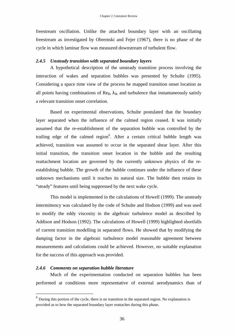
Chapter 2: Literature Review
36
freestream oscillation. Unlike the attached boundary layer with an oscillating
freestream as investigated by Obremski and Fejer (1967), there is no phase of the
cycle in which laminar flow was measured downstream of turbulent flow.
2.4.5 Unsteady transition with separated boundary layers A hypothetical description of the unsteady transition process involving the
interaction of wakes and separation bubbles was presented by Schulte (1995).
Considering a space time view of the process he mapped transition onset location as
all points having combinations of Reθ, λθ, and turbulence that instantaneously satisfy
a relevant transition onset correlation.
Based on experimental observations, Schulte postulated that the boundary
layer separated when the influence of the calmed region ceased. It was initially
assumed that the re-establishment of the separation bubble was controlled by the
trailing edge of the calmed region6. After a certain critical bubble length was
achieved, transition was assumed to occur in the separated shear layer. After this
initial transition, the transition onset location in the bubble and the resulting
reattachment location are governed by the currently unknown physics of the re-
establishing bubble. The growth of the bubble continues under the influence of these
unknown mechanisms until it reaches its natural size. The bubble then retains its
“steady” features until being suppressed by the next wake cycle.
This model is implemented in the calculations of Howell (1999). The unsteady
intermittency was calculated by the code of Schulte and Hodson (1999) and was used
to modify the eddy viscosity in the algebraic turbulence model as described by
Addison and Hodson (1992). The calculations of Howell (1999) highlighted shortfalls
of current transition modelling in separated flows. He showed that by modifying the
damping factor in the algebraic turbulence model reasonable agreement between
measurements and calculations could be achieved. However, no suitable explanation
for the success of this approach was provided.
2.4.6 Comments on separation bubble literature Much of the experimentation conducted on separation bubbles has been
performed at conditions more representative of external aerodynamics than of
6 During this portion of the cycle, there is no transition in the separated region. No explanation is provided as to how the separated boundary layer reattaches during this phase.
Chapter 2: Literature Review
37
turbomachinery environments. Low turbulence levels are typically used, and bubbles
have typically been at the leading edge rather than on the rear surface as found in low-
pressure turbines. Additionally little attention has been paid to measurements of the
transition process in the shear layer with the only appropriate measurements being
those of Malkiel and Mayle (1995).
The effects of wake passing on separation bubbles has been investigated by
Schulte (1995) and Howell (1999) who highlighted the importance of the wake
passing in reducing the losses as a result of suppressing the separation bubble. The re-
establishment of the bubble and transition processes that occurs in the unsteady
bubble and re-establishing bubble has not been investigated.
2.5 Concluding remarks The body of literature concerning unsteady transition in turbomachines is
growing rapidly, however, understanding of basic transition processes in engineering
applications remains incomplete. The advent of direct simulations of simple turbulent
and transitional processes promises to provide data of unprecedented resolution and
detail, however the interpretation, understanding and translating of this data into
practical engineering design correlations remains a challenge which must be based on
an understanding of the fundamental physics governing the transition process.
This thesis seeks to unveil the dominant mechanisms that govern the transition
process that results from the interaction of a turbulent wake and highly decelerated,
separating, boundary layer. It does not intend to add to the list of transition
correlations, but rather through a series of experimental investigations to describe the
interaction mechanism thereby paving the way for future modelling efforts.
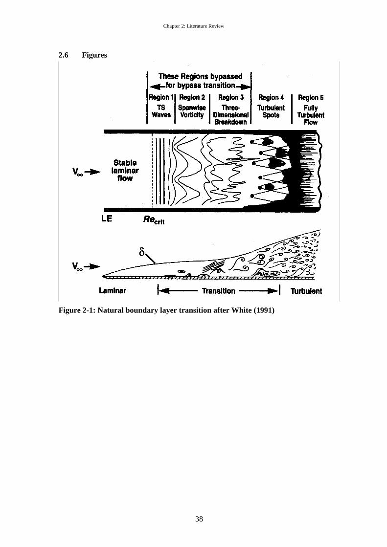
Chapter 2: Literature Review
38
2.6 Figures
Figure 2-1: Natural boundary layer transition after White (1991)
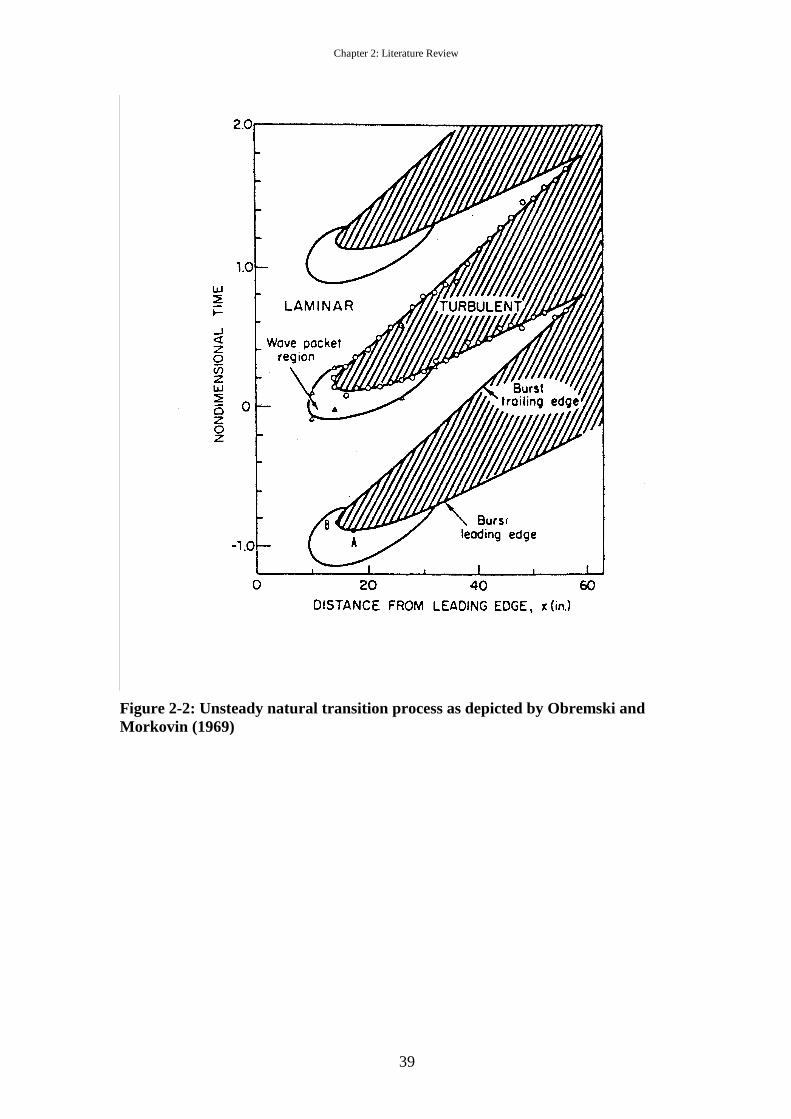
Chapter 2: Literature Review
39
Figure 2-2: Unsteady natural transition process as depicted by Obremski and Morkovin (1969)
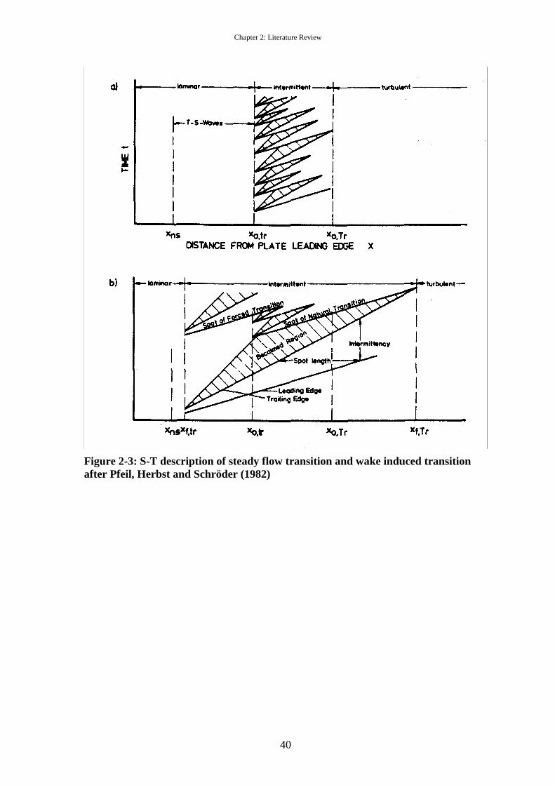
Chapter 2: Literature Review
40
Figure 2-3: S-T description of steady flow transition and wake induced transition after Pfeil, Herbst and Schröder (1982)
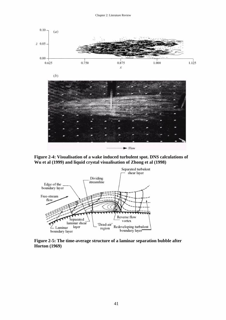
Chapter 2: Literature Review
41
Figure 2-4: Visualisation of a wake induced turbulent spot. DNS calculations of Wu et al (1999) and liquid crystal visualisation of Zhong et al (1998)
Figure 2-5: The time-average structure of a laminar separation bubble after Horton (1969)
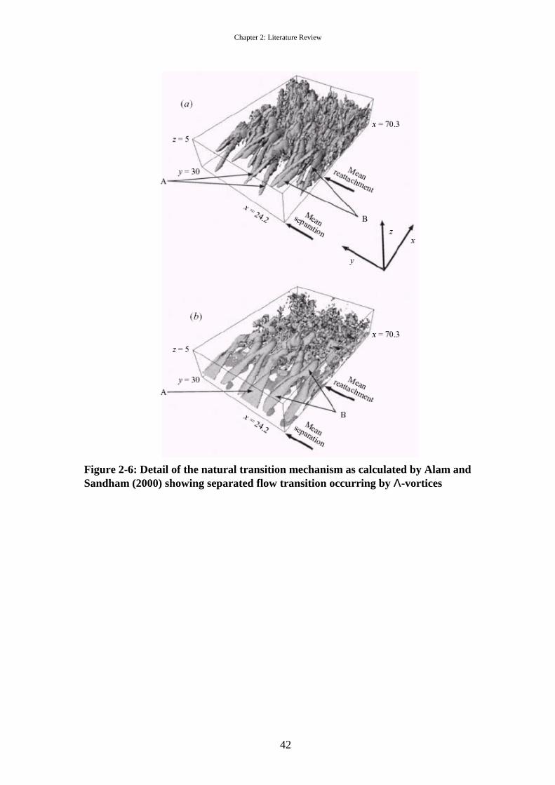
Chapter 2: Literature Review
42
Figure 2-6: Detail of the natural transition mechanism as calculated by Alam and Sandham (2000) showing separated flow transition occurring by Λ-vortices
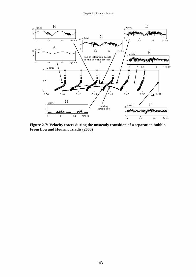
Chapter 2: Literature Review
43
Figure 2-7: Velocity traces during the unsteady transition of a separation bubble. From Lou and Hourmouziadis (2000)
44
Chapter 3: Experimental Methods
3.1 Introduction The experimental facilities, instrumentation and measurements techniques
used in obtaining the experimental results presented in subsequent Chapters of this
thesis are described here. Experimental work was performed on two experimental
configurations. The first, a flat plate with an imposed pressure distribution and the
second a low-pressure (LP) turbine cascade designated T106. Both these
configurations were subjected to wakes shed from moving bar wake generators and
were attached to an exit of the Duplex wind tunnel in the Whittle Laboratory of
Cambridge University Engineering Department.
The data logging equipment is described together with details of the
instrumentation. The measurements techniques used included conventional and fast-
response static pressure measurements together with a single hot wire anemometer, a
laser Doppler anemometer and a particle image velocimetry system.
3.2 Experimental facilities
3.2.1 Wind tunnel The Duplex wind tunnel, sketched in Figure 3-1, is of an open return design
and has two exits. Air is drawn in from the laboratory by a centrifugal fan. It then
diffuses over a series of splitter plates into a constant area duct where it is diverted to
one of the two exits. Each of the ducts contains a series of grids, gauzes and
honeycombs to smooth and settle the flow before passing through a 3.7:1 area ratio
contraction and discharging into the test section.
The centrifugal fan is driven by a 75 BHP AC motor. Control of air speed is
achieved by a combination of fan speed and inlet throttle position.
3.2.2 Bar passing flat plate The experimental facility, shown in Figure 3-2, consists of an aluminium plate
545mm long by 458mm wide and 30mm thick. A 8:3 ellipse was used for the leading
edge and the trailing edge of the plate was blunt. A splitter plate 100mm in length was
attached to the centre of the trailing edge to suppress vortex shedding. The flat plate
was mounted in a wooden box of constant span with a glass window to provide
optical access for the LDA measurements. A pair of contoured walls was mounted in

Chapter 3: Experimental Methods
45
the box to impose a pressure distribution on the flat plate. A symmetrical arrangement
was chosen to ensure zero incidence at the leading edge. The shape of the contoured
walls was designed using a simple one-dimensional continuity argument to match the
pressure distribution measured on the flat plate to that measured by Cicatelli (1998)
on the T106 LP turbine cascade.
A moving bar wake generator was used to create unsteady wake passing
conditions. Carbon fibre bars of 7.8mm diameter were attached to a pair of reinforced
nylon belts. The belts of the wake generator were driven by a speed controlled 2 HP
DC motor. The belts travelled on 4 sets of pulleys so that the bars passed across the
inlet of the test section and then around the outside of a wooden box containing the
flat plate and contoured end-walls. The return path of the bars was well downstream
of the test section so that no downstream effect of the bar passing was generated. The
bars passed 250mm in front of the plate leading edge. As the bars passed across the
inlet of the test section, they shed wakes, which convect over the flat plate and
simulate the wake passing conditions in a turbomachine.
3.2.3 Bar passing cascade The bar passing cascade facility, shown in Figure 3-3, is a cascade analogue of
a multi-stage turbomachine. The facility has previously been described by Banieghbal
et al (1995) and Schulte (1995).
The wakes shed from upstream blade rows in a real machine are simulated by
an array of cylindrical bars moving across the inlet plane of the cascade. Pfeil and
Eifler (1976) have shown that the far wake region of a cylindrical bar (x/d>80) is
representative of the wakes in a real turbomachine. The bar passing cascade provides
no means of representing the correct potential filed of adjacent blade rows.
The bars are held between two nylon belts that run on two sets pulleys. The
pulley system is driven through a belt drive by a 2.0 HP DC motor, the speed of
which is manually controlled by a variac. The range of reduced frequencies that the
rig is capable of simulating is limited by the positioning of the lugs on the nylon belts.
The configuration of the bar passing cascade required that the top and bottom
walls of the cascade be slotted to permit the passage of wake generator bars (Figure
3-4). These slots provide two additional passages to the flow. The slot on the top wall
does not present a problem, as it requires the flow to change direction, however, the

Chapter 3: Experimental Methods
46
slot on the bottom wall was more closely aligned with the flow. Moreover, the
pressure gradient due to the incidence of the cascade forces flow out of the bottom
slot. The result is an effective increase of incidence on the cascade and a non-uniform
inlet static pressure. In order to minimise this problem and maintain inlet periodicity,
an additional dummy passage was created on the suction side of the cascade as shown
in Figure 3-4. This was achieved by adding a straight flap to the bottom wall. The
throat of this dummy passage was then adjusted so that the combined throat of the end
wall gap and the dummy passage matched that of one of the cascade passages. The
flap of the dummy passage was set while monitoring the inlet static pressure and
thereby ensuring periodicity. The periodicity of inlet static pressure was maintained
within a 2.5% range of inlet dynamic head.
3.2.4 T106 low pressure turbine cascade The cascade investigated is designated T106. The profile is that of an aft-
loaded low-pressure turbine blade. Blade co-ordinates together with blade static
pressure tapping locations are presented in Appendix I. The cascade used consisted of
5 blades of chord 198mm. Details of the cascade are presented in Table 3-1.
The bar passing conditions were chosen to represent a repeating stage of the
T106 profile at 50% reaction. The flow coefficient for this condition is φ=0.83. The
Reynolds number based on chord and exit velocity for the datum test case was
Re2C=1.6×10⁵.
Number of blades 5 Chord [mm] 198 Axial chord [mm] 170 Blade stagger [°] 59.3 Pitch [mm] 158 Span [mm] 375 Suction surface length [mm] 264.7 Pressure surface length [mm] 230.0 Inlet flow angle [°] 37.7 Design exit flow angle [°] 63.2 Bar diameter [mm] 2.05 Bar Pitch [mm] 158 & 316 Axial distance: bars to LE [mm] 70 Flow Coefficient (φ=Vx/Ub) 0.83
Table 3-1: Specification of T106 cascade.

Chapter 3: Experimental Methods
47
3.2.5 Artificial disturbance generator Artificial disturbances were generated in the boundary layer of one of the
T106 turbine blades by a puff of air emerging through a small hole in the blade
surface. The disturbance generator, sketched in Figure 3-5, consisted of a signal
generator, a 30W power amplifier and a 40W, 4Ω loudspeaker attached to a sheet of
Perspex as shown in the sketch. A stainless steel tube was mounted through the
Perspex sheet so that when the diaphragm of the speaker moved a jet of air would be
forced out of the tube. A PVC tube was used to connect the outlet of the disturbance
generator to a 0.3mm hole drilled in the surface of the turbine blade.
The disturbance generator was driven by a square wave of 5µs duration that
was generated at the desired frequency by a Thandar TG503 Function generator. The
jet emerging from the blade surface was sufficient to disturb the boundary layer.
3.3 Instrumentation
3.3.1 Data logging All data logging was controlled by a PC running LabVIEW software. Voltages
were acquired using a National Instruments PCI-MIO-16E-1 card, which consisted of
a 12 bit A/D converter with a maximum throughput of 1.25 MS/s multiplexed onto 16
analogue input channels. A National Instruments BNC 2090 connector panel was used
to connect BNC cables to the data acquisition board.
The traverse gear consisted of Unislide traverse slides driven by McLennan
stepper motors. The stepper motors were driven by Digiplan CD25 stepper motor
drivers and controlled by a Digiplan IFX indexer system. The PC communicated with
the Digiplan system by a RS232 serial network.
A Scanivalve DSA 3017 with ±10 inH2O range was used to provide up to 16
simultaneous pressures measurements to monitor the experimental flow conditions.
The PC communicated with the DSA over a network using TCP/IP communication.
Tunnel total temperature was logged with a total temperature probe and a T-
type thermocouple. A Farnell DTT2 Digital Thermocouple Thermometer was used to
precondition the thermocouple output. The PCI-MIO-16E-1 card measured the
thermometer’s analogue output voltage. Atmospheric pressure was measured using a
Druk DPI250 absolute pressure indicator the analogue output voltage was again
logged by the PCI-MIO-16E-1 card. Bar passing speed was monitored with a
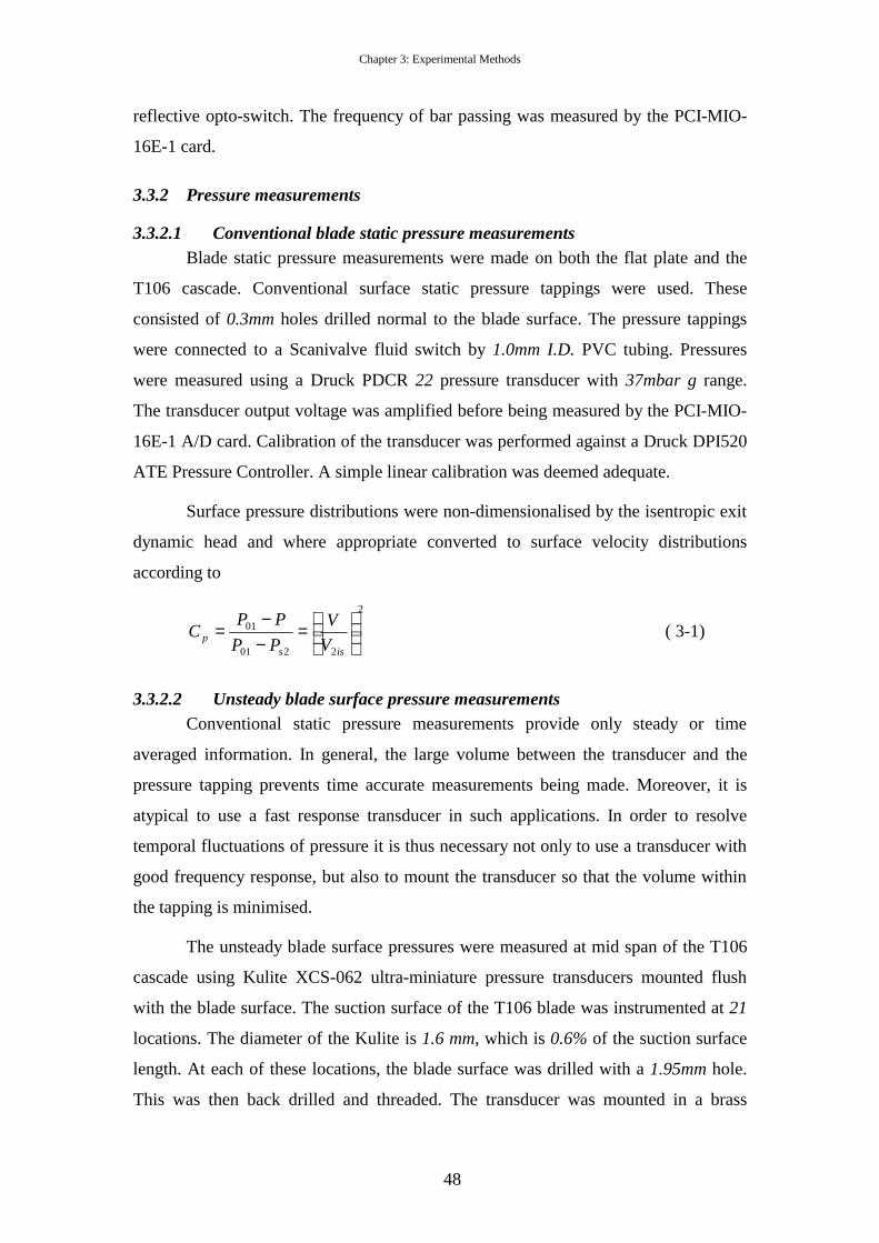
Chapter 3: Experimental Methods
48
reflective opto-switch. The frequency of bar passing was measured by the PCI-MIO-
16E-1 card.
3.3.2 Pressure measurements
3.3.2.1 Conventional blade static pressure measurements Blade static pressure measurements were made on both the flat plate and the
T106 cascade. Conventional surface static pressure tappings were used. These
consisted of 0.3mm holes drilled normal to the blade surface. The pressure tappings
were connected to a Scanivalve fluid switch by 1.0mm I.D. PVC tubing. Pressures
were measured using a Druck PDCR 22 pressure transducer with 37mbar g range.
The transducer output voltage was amplified before being measured by the PCI-MIO-
16E-1 A/D card. Calibration of the transducer was performed against a Druck DPI520
ATE Pressure Controller. A simple linear calibration was deemed adequate.
Surface pressure distributions were non-dimensionalised by the isentropic exit
dynamic head and where appropriate converted to surface velocity distributions
according to
2
2201
01
=
−−
=iss
p V
V
PP
PPC ( 3-1)
3.3.2.2 Unsteady blade surface pressure measurements Conventional static pressure measurements provide only steady or time
averaged information. In general, the large volume between the transducer and the
pressure tapping prevents time accurate measurements being made. Moreover, it is
atypical to use a fast response transducer in such applications. In order to resolve
temporal fluctuations of pressure it is thus necessary not only to use a transducer with
good frequency response, but also to mount the transducer so that the volume within
the tapping is minimised.
The unsteady blade surface pressures were measured at mid span of the T106
cascade using Kulite XCS-062 ultra-miniature pressure transducers mounted flush
with the blade surface. The suction surface of the T106 blade was instrumented at 21
locations. The diameter of the Kulite is 1.6 mm, which is 0.6% of the suction surface
length. At each of these locations, the blade surface was drilled with a 1.95mm hole.
This was then back drilled and threaded. The transducer was mounted in a brass

Chapter 3: Experimental Methods
49
sheath, which was screwed into the holes in the blade until the transducer was flush
with the surface as shown in Figure 3-6. Brass plugs were made for each of the
unused tapping locations and were polished flush with the surface of the blade.
Conventional static pressure tapings located at 25% span and the same surface
location were used to measure the mean pressure levels at each of the Kulite
locations.
Up to four Kulite transducers were used simultaneously, each powered by a
Fylde 492BBS bridge with 12V excitation. The bridge output signals were amplified
by Fylde 254GA amplifiers with a gain of 1000. The voltage out of the amplifiers was
measured by the PCI-MIO-16E-1. The input range was set to ±0.2V. The Kulites were
used to measure only the pressure fluctuations and not mean levels. It was thus
possible to use a Fylde 294-OA auto-zero control unit to zero the bridge outputs
before each acquisition thereby minimising thermal drift.
Calibration of the transducers, bridges and amplifiers of all four Kulites was
performed simultaneously using the DPI520 as a common pressure source. The
calibration thus included a calibration of the amplifiers and bridges. The response of
the transducers and amplifiers was linear and, as the mean level was not required from
the Kulites, only the slope of the calibration curve was retained. The system described
above resulted in a sensitivity of approximately 500Pa/V with a discretisation error of
0.05Pa. Each measurement consists of 256 ensembles of 4096 points logged at
10Khz.
The mean pressure level was measured using a Scanivalve DSA 3017 array
with a ±10 in H2O range and 16-bit A/D. The discretisation error on this measurement
is thus 1.0 Pa which corresponds to 1.0% exit dynamic head at Re2C=1.6×10⁵.
Processing of the resulting signals to achieve a pressure trace required the
mean and fluctuating components of the signals to be combined. The fluctuating
component was obtained by applying the linear calibration to each voltage ensemble.
The mean level was then subtracted to provide a zero-mean pressure ensemble. These
were then ensemble averaged before adding the mean level measured by the DSA to
give the final ensemble averaged pressure trace. The results were non-
dimensionalised by isentropic exit dynamic head to give the ensemble averaged
pressure coefficient.
Chapter 3: Experimental Methods
50
3.3.3 Hot wire measurements Hot wire boundary layer traverses were performed on the T106 cascade using
a Dantec 55P15 single wire boundary layer probe with 5µm × 1mm tungsten element
set to an overheat ratio of 1.8. A Dantec 56C01 constant temperature anemometer was
used in conjunction with a Dantec 56C17 bridge and a Dantec 55N22 signal-
conditioning unit.
The raw unfiltered output of the anemometer was typically between 1.4V and
2.5V. This signal was logged by the PCI-MIO-16E-1 with a range of 0-5V to provide
a mean DC signal level. The AC component of the signal was obtained separately by
band pass filtering the signal between 1Hz and 10KHz. The resulting signal was in the
range ±0.5V and was logged by the PCI-MIO-16E-1. The signal was then
reconstructed by adding the DC level to the zero-mean filtered output thereby
enhancing the signal resolution. The hot wire measurements presented in this thesis
consists of 128 ensembles of AC data and 16 ensembles of DC data. Each ensemble
consists of 4096 points logged at 10KHz.
Positioning of the probe in the stream wise direction was performed manually.
The location of the wall was then found by measuring the electrical contact between
the probe7 and the blade surface using a circuit as shown in Figure 3-7. To do this a
voltage source was connected between the probe and the blade surface. With no
contact, the full supply voltage was measured between the probe and the blade
surface, whereas upon contact the measured output voltage was zero. The surface
locating procedure was performed automatically by traversing the probe towards the
surface in steps of 0.05mm until the average measured voltage dropped to 90% of the
no-contact value. This location was then taken to be the blade surface. Probe and rig
vibration were accounted for by performing the wall location procedure at the
operating condition.
Calibration of the hot wire probes described above was performed in a suction
calibration facility. In order to account for temperature drift effects the flow
temperature was measured at each calibration point. Ten calibration points,
7 In order to prevent damage to the probe the anemometer was switched off during this process. The wire element demonstrates greater strength when cold.

Chapter 3: Experimental Methods
51
encompassing the velocities to be measured, were used in the calibration. A best-fit
calibration for King’s law was then found.
The correction of Cox (1957) was applied to the measured data to account for
the effects of heat transfer to the metal surfaces. To achieve this a unique no-flow
traverse was performed at each measurement location. The correction of Bearman
(1971) was applied to account for drift in air temperature using the measured inlet
flow temperature.
3.3.4 Laser Doppler anemometry The Doppler effect is a frequency shift in radiation received from one body
moving relative to another. Laser Doppler Anemometry (LDA) uses this effect to
measure the velocity of particles suspended in a fluid. If the particles follow the fluid
faithfully then the velocity of the particle is a reliable measure of the flow velocity.
For measurements of incompressible airflow, the Doppler effect is not used
directly as the comparatively small velocity of the particles relative to that of the
incident light means that the technique is insensitive. Rather, two coherent laser
beams, typically from the same source, are focused to a common point. Particles
passing through the intersection volume scatter light from each beam at a slightly
different frequency due to the differences in angles of the incident light on the
particle. The beat frequency8 can then be used to find the velocity of the particle. The
velocity measured by LDA is the component of velocity in the plane of the
intersecting beams
The measurements reported in Chapter 4 of this thesis used a single
component LDA system. However, upon the acquisition of a second component, the
2D system, consisting of two pairs of intersecting beams and two signal processors,
was used. Two components of the velocity vector can thus be simultaneously
measured when a particle passes the common intersection volume of the two pairs of
beams.
The LDA system is sketched in Figure 3-8. Light was supplied by a 5W
Argon-Ion laser (Coherent Innova 70C). The transmitting optics consisted of a Dantec
FibreFlow unit incorporating a colour separator and Bragg cell. A 2D 85mm Dantec
8 The beat frequency is the interference frequency resulting from the difference in frequency between light scattered from the two beams.
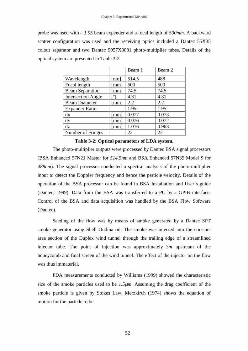
Chapter 3: Experimental Methods
52
probe was used with a 1.95 beam expender and a focal length of 500mm. A backward
scatter configuration was used and the receiving optics included a Dantec 55X35
colour separator and two Dantec 9057X0081 photo-multiplier tubes. Details of the
optical system are presented in Table 3-2.
Beam 1 Beam 2
Wavelength [nm] 514.5 488 Focal length [mm] 500 500 Beam Separation [mm] 74.5 74.5 Intersection Angle [º] 4.31 4.31 Beam Diameter [mm] 2.2 2.2 Expander Ratio 1.95 1.95 dx [mm] 0.077 0.073 dy [mm] 0.076 0.072 dz [mm] 1.016 0.963 Number of Fringes 22 22
Table 3-2: Optical parameters of LDA system.
The photo-multiplier outputs were processed by Dantec BSA signal processors
(BSA Enhanced 57N21 Master for 514.5nm and BSA Enhanced 57N35 Model S for
488nm). The signal processor conducted a spectral analysis of the photo-multiplier
input to detect the Doppler frequency and hence the particle velocity. Details of the
operation of the BSA processor can be found in BSA Installation and User’s guide
(Dantec, 1999). Data from the BSA was transferred to a PC by a GPIB interface.
Control of the BSA and data acquisition was handled by the BSA Flow Software
(Dantec).
Seeding of the flow was by means of smoke generated by a Dantec SPT
smoke generator using Shell Ondina oil. The smoke was injected into the constant
area section of the Duplex wind tunnel through the trailing edge of a streamlined
injector tube. The point of injection was approximately 3m upstream of the
honeycomb and final screen of the wind tunnel. The effect of the injector on the flow
was thus immaterial.
PDA measurements conducted by Williams (1999) showed the characteristic
size of the smoke particles used to be 1.5µm. Assuming the drag coefficient of the
smoke particle is given by Stokes Law, Merzkirch (1974) shows the equation of
motion for the particle to be
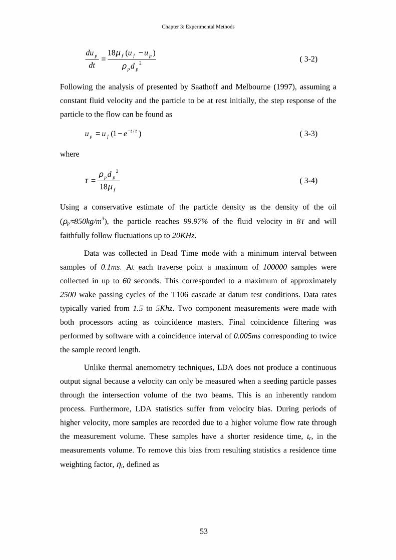
Chapter 3: Experimental Methods
53
2
)(18
pp
pffp
d
uu
dt
du
ρ
µ −= ( 3-2)
Following the analysis of presented by Saathoff and Melbourne (1997), assuming a
constant fluid velocity and the particle to be at rest initially, the step response of the
particle to the flow can be found as
)1( /τtfp euu −−= ( 3-3)
where
f
ppd
µρ
τ18
2
= ( 3-4)
Using a conservative estimate of the particle density as the density of the oil
(ρp≈850kg/m3), the particle reaches 99.97% of the fluid velocity in 8τ and will
faithfully follow fluctuations up to 20KHz.
Data was collected in Dead Time mode with a minimum interval between
samples of 0.1ms. At each traverse point a maximum of 100000 samples were
collected in up to 60 seconds. This corresponded to a maximum of approximately
2500 wake passing cycles of the T106 cascade at datum test conditions. Data rates
typically varied from 1.5 to 5Khz. Two component measurements were made with
both processors acting as coincidence masters. Final coincidence filtering was
performed by software with a coincidence interval of 0.005ms corresponding to twice
the sample record length.
Unlike thermal anemometry techniques, LDA does not produce a continuous
output signal because a velocity can only be measured when a seeding particle passes
through the intersection volume of the two beams. This is an inherently random
process. Furthermore, LDA statistics suffer from velocity bias. During periods of
higher velocity, more samples are recorded due to a higher volume flow rate through
the measurement volume. These samples have a shorter residence time, tr, in the
measurements volume. To remove this bias from resulting statistics a residence time
weighting factor, ηi, defined as

Chapter 3: Experimental Methods
54
∑=
=N
jjr
iri
t
t
1
η ( 3-5)
was employed (George, 1975). Ensemble averaging of the LDA data was performed
by first dividing the wake passing period into a number of time bins (typically 128
were used). The weighting factor, mean, variance and cross moments were then
assembled for each of these time bins according to
∑=
=N
iiiuu
1
η ( 3-6)
∑=
−=N
iii uuu
1
22 )(' η ( 3-7)
∑=
−−=N
iiii vvuuvu
1
))(('' η ( 3-8)
Positioning of the measuring volume in the stream-wise direction was
performed manually. The location of the surface was then found in a manner similar
to that described for the hot wire boundary layer measurements. The probe was
traversed towards the surface in steps of 0.05mm. The pedestal signal9 of the BSA was
then logged by the PCI-MIO-16E-1. The wall was identified as the position where the
pedestal signal reached a peak value. This corresponds to the position where the
photo-multiplier receives the most reflected light due to the measuring volume
intersecting the wall. Locating the wall was performed with the laser at low power to
prevent the anode limiter10 from becoming active.
3.3.5 Digital particle image velocimetry Particle image velocimetry (PIV) is essentially a quantitative flow
visualisation technique. Two images of a seeded flow are captured at a known time
interval. By tracking the movement of the seeding particles between the two images it
is possible to calculate the velocity of the particles and from this, assuming that the
particles faithfully follow the fluid, to measure the fluid velocity field.
9 The pedestal signal is a low pass filtered version of the photo-multiplier signal available at a BNC connector on the front of the BSA signal processor. 10 The anode limiter limits the current supplied to the photo-multiplier to prevent damage to the receiver. This is a hardware feature of the BSA

Chapter 3: Experimental Methods
55
The digital PIV technique used here uses a digital video camera to acquire
images of the seeded flow that is illuminated by a laser light sheet. Two lasers are
used and their pulses are synchronised with the ‘shutter’ of the digital camera so that
the laser pulses are captured by successive frames of the digital camera. This greatly
reduces the time between images allowing higher speed flows to be captured.
A commercial TSI PIV system was used consisting of a pair of 50mJ New
Wave Nd-YAG lasers, a synchroniser and a Kodak digital camera with 1024×1024
CCD array. A 105mm Nikon lens was used and zoomed to provide a 19.0mm square
field of view. The Nd-YAG laser light was transmitted to the light sheet optics
through an articulated delivery arm. The light sheet was generated at the end of the
articulated arm by a 25.4mm focal length negative cylindrical lens and a 500mm focal
length spherical lens. This arrangement provided a light sheet between 0.5mm and
1.5mm thick on the blade surface, which was approximately 500mm from the light
sheet optic. The light sheet covered approximately half a blade passage.
The layout of the experiment is shown in the sketch of Figure 3-9. The light
sheet was positioned downstream of the cascade pointing upstream and onto the rear
portion of the suction surface. The position of the light sheet optic was chosen so that
shadows from the returning bars of the wake generator were not present at the phases
of interest. The light sheet optic was also positioned out of the main exit flow to
minimise blockage effects. The camera was positioned to look parallel to the blade
surface through the glass sidewall that was used for the LDA measurements.
The flow was seeded with a mist of groundnut oil generated by a pair of TSI
Six-Jet Atomisers used in parallel. The seeding was introduced into the wind tunnel
approximately 3m upstream of the bar passing cascade, at the same point in the wind
tunnel as the smoke used for the LDA.
The inter frame delay was set to ∆t=3µs, which gave particle displacements in
the range –3 to 6 pixels. The maximum data rate of the PIV system was 15Hz so it
was not possible to capture a sequence of images within one bar passing cycle. The
acquisition of images was thus triggered. The trigger used for the LDA measurements
was passed through a delay generator thereby allowing the PIV images to be acquired
at different phases relative to the trigger.

Chapter 3: Experimental Methods
56
Processing of the acquired image pairs was done with LaVision’s DaVis
V.6.03 software (LaVision, 2001)11. An adaptive multi-pass technique was used with
the initial cell size of 64×64 pixels decreasing to a final cell size of 16×16 pixels with
a spatial resolution of 304µm×304µm. The final cells were overlapped by 50%
effectively increasing the data yield and giving a vector grid spacing of 152µm.
11 Processing of the acquired image pairs was not done by the author but by Mr D Hollis of Loughborough University. His assistance is gratefully acknowledged.
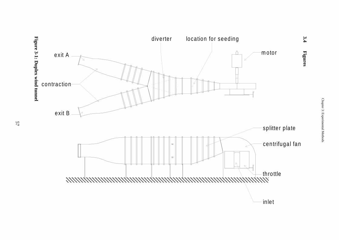
Ch
ap
ter 3: E
xperim
enta
l Meth
ods
57
3.4 F
igures
m otor
th ro ttle
contrac tion
d iverter
cen trifuga l fan
exit A
sp litte r p la te
in le t
ex it B
location fo r seed ing
Figure 3-1: D
uplex wind tunnel
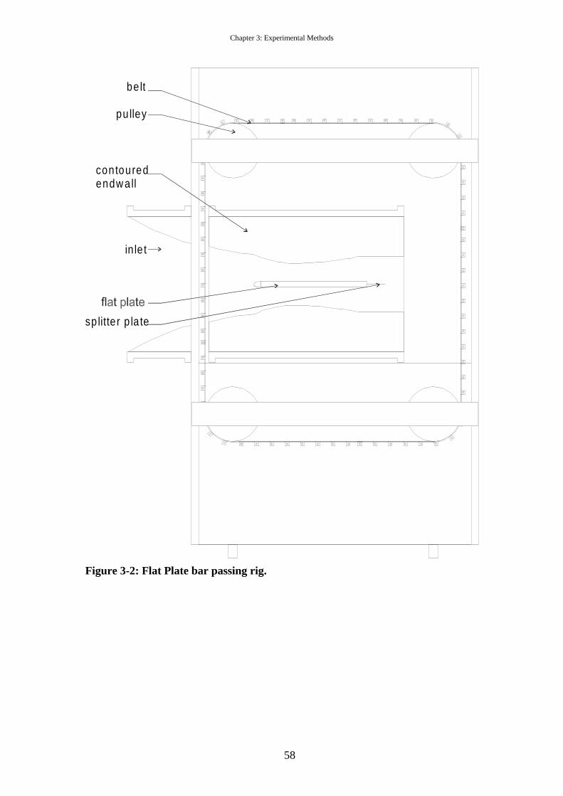
Chapter 3: Experimental Methods
58
contouredendw all
sp litte r p la te
pu lley
be lt
in le t
Figure 3-2: Flat Plate bar passing rig.
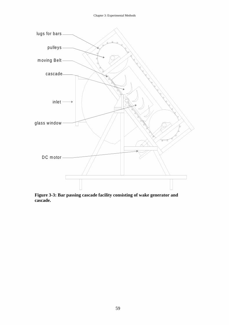
Chapter 3: Experimental Methods
59
in le t
cascade
m oving Be lt
pu lleys
D C m otor
lugs for bars
g lass w indow
Figure 3-3: Bar passing cascade facility consisting of wake generator and cascade.
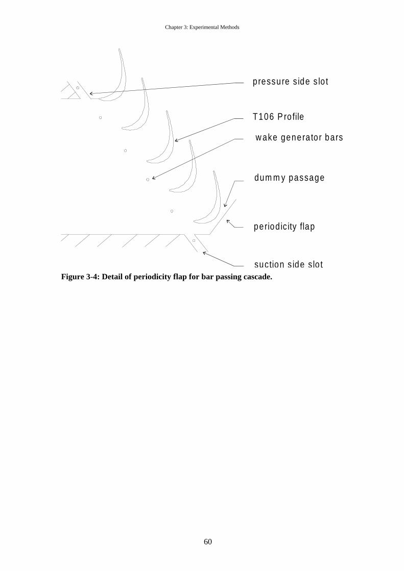
Chapter 3: Experimental Methods
60
period ic ity flap
suction s ide s lo t
dum m y passage
T106 P ro file
w ake genera to r bars
pressure s ide s lo t
Figure 3-4: Detail of periodicity flap for bar passing cascade.
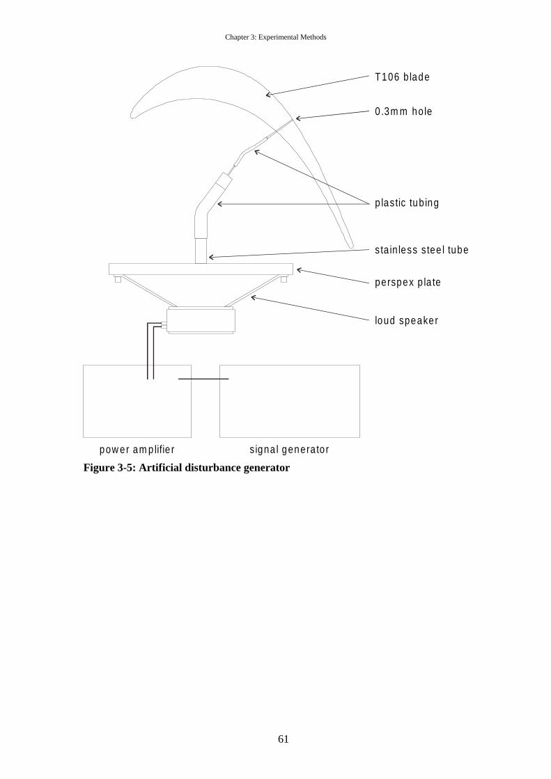
Chapter 3: Experimental Methods
61
s igna l generato rpow er am p lifie r
loud speaker
perspex p la te
0 .3m m hole
T106 b lade
p lastic tub ing
sta in less s tee l tube
Figure 3-5: Artificial disturbance generator
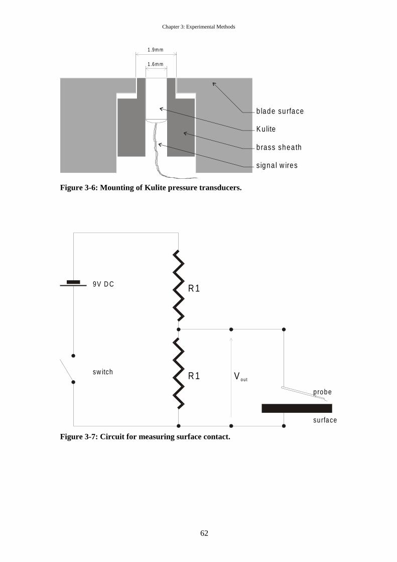
Chapter 3: Experimental Methods
62
b lade su rface
K ulite
b rass shea th
s igna l w ires
1 .6m m
1.9m m
Figure 3-6: Mounting of Kulite pressure transducers.
9V D C R 1
probe
surface
R 1 V o utsw itch
Figure 3-7: Circuit for measuring surface contact.
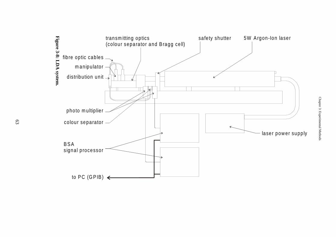
Ch
ap
ter 3: E
xperim
enta
l Meth
ods
63
d is tribu tion un it
m an ipu la to r
transm itting op tics(co lou r sepa ra to r and B ragg ce ll)
sa fe ty shu tte r 5W A rgon -Ion laser
co lour sepa ra to r
pho to m u ltip lie r
fib re op tic cab les
lase r pow er supp ly
to P C (G P IB )
B S A s igna l p rocessor
Figure 3-8: LD
A system
.
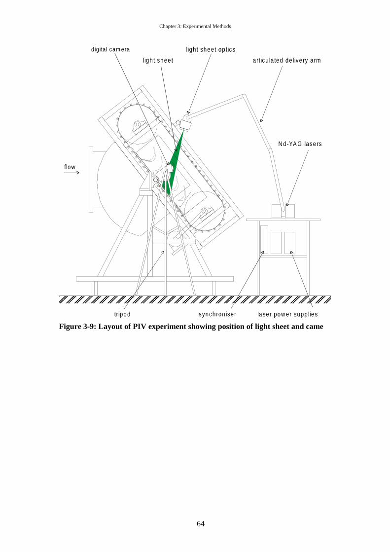
Chapter 3: Experimental Methods
64
articu la ted de live ry a rm
N d-YA G lasers
laser pow er supp liessynchron ise r
d ig ita l cam era
tripo d
ligh t shee t
ligh t shee t op tics
flow
Figure 3-9: Layout of PIV experiment showing position of light sheet and came
65
Chapter 4: The interaction of wakes with the separating boundary layer on a flat plate
4.1 Introduction This chapter presents ensemble averaged boundary layer measurements made
using the rotated 1D LDA technique detailed in Appendix II. The measurements were
performed on a flat plate subject to wakes from a moving bar wake generator. The
pressure distribution on the flat plate was matched to that measured on the T106 LP
turbine cascade.
This chapter first establishes the extent to which the flat plate is able to
simulate the cascade boundary layer. Thereafter, the unsteady boundary layer results
are presented in terms of space-time (S-T) diagrams of the integral boundary layer
parameters. All such diagrams present one period of ensemble-averaged data copied
onto two or three periods to aid interpretation. The S-T diagrams summarise the
boundary layer measurements and allow a description of the boundary layer
parameters as a function of both time and surface distance. The boundary layer
measurements are then analysed to identify the transition mechanisms between wake
passing events. The measured Reynolds stresses are also used to calculate the
boundary layer dissipation allowing the loss generating and loss reducing mechanisms
associated with unsteady transition to be identified.
Between wake passing events the boundary layer profiles slowly relax from
their turbulent shape. The calmed region that follows the turbulent boundary layer
gives way to a separating boundary layer under the influence of an adverse pressure
gradient. The transition process that occurs during this stage of the wake passing cycle
is identified to be by means of deterministic wave-like structures having a frequency
that is characteristic of Tollmien-Schlichting waves. The measurements presented
provide experimental evidence of ensemble-averaged natural transition phenomena
arising in the unsteady wake-induced transition cycle.
The boundary layer dissipation is calculated from the measurements of
Reynolds stresses and ensemble average velocity profiles. Previous claims of the
benign character of the calmed region are supported. The calmed region is found to
persist through the early stages of the separating boundary layer. Elevated levels of
loss in the unsteady wake induced turbulent boundary layer were also measured. The
Chapter 4: The interaction of wakes with the separating boundary layer on a flat plate
66
measured dissipation coefficient provides an unprecedented description of the loss
associated with the different phases of the wake separation bubble interaction from
experimental data.
4.2 Experimental details
4.2.1 Matching flat plate and cascade boundary layers The boundary layer that forms on the surface of a turbine blade is most
strongly influenced by the velocity distribution along the blade surface and the
balance of inertial to viscous forces as characterised by the Reynolds number. The
effect of surface curvature on the blade boundary layer is to introduce wall normal
pressure gradients, but these may be neglected if the boundary layer thickness is much
smaller than the radius of curvature of the surface (White, 1991). This is indeed the
case for LP turbine blades. Thus to reproduce the boundary layer of the turbine
cascade on a flat plate it is necessary to match the Reynolds number of the flow and
the surface velocity distribution.
The surface velocity distribution measured on a turbine blade results from the
combined effect of changes in flow area and curvature as the flow is accelerated and
turned by the blade row. Thus to reproduce a turbine blade velocity distribution on a
flat plate, where there is no curvature, it is necessary to use variations in flow area.
This may be achieved in practice by applying a simple one-dimensional continuity
argument to vary the area between the flat plate and a contoured end wall and thus to
achieve the desired velocity distribution. This simple argument, with no modifications
for the effects of blockage due to the boundary layer growth or curvature of the upper
wall, was used to design the shape of a pair of symmetrical end walls used to impose a
pressure gradient on the flat plate described in Chapter 3. The validity of this method
is confirmed by results presented in section 4.2.3 below.
4.2.2 Modelling the unsteady flow conditions for the flat plate The flow in real turbomachines is unsteady with convected disturbances from
upstream components and potential disturbances from both upstream and
downstream. The predominant unsteady effects on the blade surface boundary layers
are due to the convection of wakes shed from upstream blade rows. This unsteady
interaction is termed a rotor-stator interaction and may be simulated in a cascade
Chapter 4: The interaction of wakes with the separating boundary layer on a flat plate
67
environment by a moving bar wake generator (Schulte (1995), Banieghbal et al
(1995), Curtis et al (1996)).
The kinematics of the rotor-stator interaction is primarily governed by the
velocity triangles and, according to Schulte and Hodson (1998), may be simulated in a
cascade by matching the flow coefficient
b
x
U
V=φ ( 4-1)
In converting the geometry of a bar passing cascade experiment to a flat plate,
it is not possible to correctly match the wake kinematics over the whole plate due to
differences in the angle between the convecting wake and the plate surface. The
symmetrical arrangement of the flat plate experiment also lacks the circulation due to
the blade loading. However, the region of interest for this investigation is the rear of
the suction surface where the separation bubble is located. In LP turbine blade
profiles, this region has little curvature. Thus for the flat plate, the flow coefficient
was based on bar speed and exit velocity and was chosen to be representative of a
repeating stage of the T106 profile so that φ=0.83.
The reduced frequency
isr V
fCf
2
= ( 4-2)
is the ratio of the convection time scale (t=C/V2is) to the wake passing time scale
(t=1/f) and provides an indicator of the unsteadiness of the flow. This parameter must
be matched if a representative flow is to be obtained. The matching of the boundary
layer is achieved through the Reynolds number. This sets the flow velocity. Matching
the flow coefficient then sets the bar speed. Thus to match the reduced frequency the
remaining parameter to be set is the bar passing frequency which, for a given bar
speed, is achieved by selecting the spacing between the bars.
Pfeil and Eifler (1976) showed that the far wake (x/d>80) of an aerofoil is
almost the same as that of a cylindrical body having the same drag. The structure of
the convected wake is thus matched by choosing the size of the bars. However, for the
measurements reported here it was believed to be more important to match the
turbulence levels at the leading edge of the flat plate to those measured by Howell
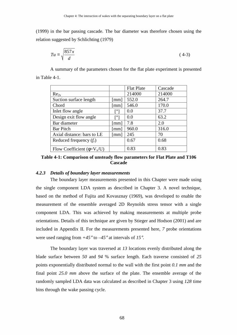
Chapter 4: The interaction of wakes with the separating boundary layer on a flat plate
68
(1999) in the bar passing cascade. The bar diameter was therefore chosen using the
relation suggested by Schlichting (1979)
d
xTu
857= ( 4-3)
A summary of the parameters chosen for the flat plate experiment is presented
in Table 4-1.
Flat Plate Cascade Re2s 214000 214000 Suction surface length [mm] 552.0 264.7 Chord [mm] 546.0 170.0 Inlet flow angle [°] 0.0 37.7 Design exit flow angle [°] 0.0 63.2 Bar diameter [mm] 7.8 2.0 Bar Pitch [mm] 960.0 316.0 Axial distance: bars to LE [mm] 245 70 Reduced frequency (fr) 0.67 0.68
Flow Coefficient (φ=Vx/U) 0.83 0.83
Table 4-1: Comparison of unsteady flow parameters for Flat Plate and T106 Cascade
4.2.3 Details of boundary layer measurements The boundary layer measurements presented in this Chapter were made using
the single component LDA system as described in Chapter 3. A novel technique,
based on the method of Fujita and Kovasznay (1969), was developed to enable the
measurement of the ensemble averaged 2D Reynolds stress tensor with a single
component LDA. This was achieved by making measurements at multiple probe
orientations. Details of this technique are given by Stieger and Hodson (2001) and are
included in Appendix II. For the measurements presented here, 7 probe orientations
were used ranging from +45° to –45° at intervals of 15°.
The boundary layer was traversed at 13 locations evenly distributed along the
blade surface between 50 and 94 % surface length. Each traverse consisted of 25
points exponentially distributed normal to the wall with the first point 0.1 mm and the
final point 25.0 mm above the surface of the plate. The ensemble average of the
randomly sampled LDA data was calculated as described in Chapter 3 using 128 time
bins through the wake passing cycle.
Chapter 4: The interaction of wakes with the separating boundary layer on a flat plate
69
4.2.4 Validation of the flat plate pressure distribution Figure 4-1 compares the velocity distribution measured on the flat plate with
steady inflow and bar passing to the measurements of Cicatelli et al (1998) for the
T106 cascade with bar passing. From this it is apparent that for the case of bar
passing, when the separation bubble is suppressed, excellent agreement was achieved
between the flat plate and cascade velocity distributions. However, for the flat plate
with steady inflow, agreement was only achieved up to the separation location and the
velocity distribution in the separated region was not perfectly matched.
The discrepancies between the flat plate and cascade velocity distributions for
steady inflow may be explained in terms of the differences in geometry between the
two cases. The displacement thickness of attached boundary layers varies slowly with
streamwise distance; however, upon separation there is a sharp increase in boundary
layer thickness. It is impossible to accurately predict the boundary layer growth after
separation. The increase in boundary layer thickness increases the boundary layer
blockage. This accelerates the freestream flow due to the change in area. Differences
between cascade and flat plate geometry do not allow the ratio of flow area to
blockage from the separated boundary layer to be conserved. The feedback
mechanisms responsible for the bubble formation are thus not reproduced. This may
account for differences.
For the case with wake passing, the time mean pressure distribution measured
on the flat plate was found to be in excellent agreement with that measured on the
T106 cascade as shown in Figure 4-1. The improvement in agreement over the steady
case is due to the periodic suppression of the separation bubble due to the wakes. This
reduces the blockage effect responsible for discrepancies in the steady flow case.
4.2.5 Validation of flat plate boundary layer Further validation, in this case using the steady pre-separation boundary layer,
is presented in Figure 4-2. High levels of agreement were achieved between integral
parameters calculated from boundary layer traverses and those calculated by the
integral method of Thwaites (see White, 1991). The integral calculation was based on
the velocity distribution measured with a tripped boundary layer to better approximate
the inviscid pressure distribution. The method of Thwaites is inaccurate near and
invalid beyond the point of laminar separation and for that reason the integration was
not continued to the trailing edge.
Chapter 4: The interaction of wakes with the separating boundary layer on a flat plate
70
4.3 Ensemble averaged measurements for wake boundary layer interaction
4.3.1 Unsteady freestream disturbance environment The convection of a wake over an aerofoil surface has been described by
Meyer (1958). His simplified model, known as the negative jet, describes the
interaction of a moving wake with a blade surface. The flow is described as the
superposition of a jet pointing towards the wake source (negative jet) on a uniform
stream. As the wake convects with the freestream, it is chopped by the blade. The
resulting wake segments behave as negative jets, which impinge on the blade suction
surface. The effect of the impinging action at a fixed location is observed first as an
acceleration of the boundary layer edge velocity as the wake approaches from
upstream. This is due to the addition of the freestream and perturbation velocity
components. After the centre of the wake passes, the perturbation component from the
impinging jet changes direction. This causes the boundary layer edge velocity to
decrease to a level below that of the undisturbed flow. As the wake continues to
convect, the impingement effect reduces and the edge velocity returns to its
undisturbed state.
The negative jet effect described above is evident in Figure 4-3. Here time
traces of the measured boundary layer edge velocity12 are plotted at several points
along the surface of the flat plate. The vertical scale is non-dimensional surface
distance at which the measurement was made. The amplitude of the traces is arbitrary
but consistent from trance to trace. Prior to the arrival of the wake, the boundary layer
edge velocity is seen to increase above the time mean value and after the passage of
the wake velocity decreases below the time mean before recovering to its undisturbed
level. This agrees with the above description of the negative jet.
The trajectory of the freestream flow is depicted in Figure 4-3 by lines A and
B. These lines were calculated from the measured time-mean velocity distribution.
The alignment of the peaks and troughs in the boundary layer edge velocities with
these trajectory lines show that the wake is simply convected with the local
freestream.
12 The boundary layer edge is defined as the point where the ensemble average velocity is 98% of the maximum measured ensemble averaged velocity in the boundary layer profile. The boundary layer edge velocity is the velocity at this point and the turbulence intensity at the boundary layer edge is the turbulence intensity at this point.

Chapter 4: The interaction of wakes with the separating boundary layer on a flat plate
71
The time delay between the peak and the trough is indicative of the wake
width. From Figure 4-3, it is apparent that the wake width is almost constant along the
length of the flat plate in the current measurements.
The boundary layer edge turbulence intensity, based on the local boundary
layer edge velocity, is plotted as an S-T diagram in Figure 4-4. Line A and line B from
Figure 4-3 have been transferred onto this plot. It is apparent that the maximum
turbulence level coincides with the center of the wake, a point approximately half way
between line A and line B. Upstream of 60% surface length the level of wake centre
line turbulence is seen to reach levels of about 5%. The undisturbed flow in the same
region has turbulence levels as low as 0.5%. After 65% surface length, the turbulence
level between wakes increases to levels of up to 3%, however the dominant region of
high turbulence is still confined to the wake centreline. A further region of high
turbulence, labelled C, arises in the region following the wake and downstream of
65% surface length. This is the result of boundary layer transition induced by the
wake passing.
4.3.2 Response of the boundary layer through a wake passing cycle Ensemble averaged velocity profiles measured at 76% surface length are
shown in Figure 4-5 and the boundary layer integral parameters calculated from the
measured ensemble average profiles through the wake passing cycle are presented in
Figure 4-6. The displacement thickness, δ*, momentum thickness, θ, and Blackwelder
thickness, δ’ , which is a measure of the turbulence in the boundary layer, were
calculated according to
dyU
yu
y∫= ∞
−=
98
0
* )(1
δ
δ ( 4-4)
dyU
yu
U
yu
y∫= ∞∞
−=
98
0
)(1
)(δ
θ ( 4-5)
∫=
+=98
0
2221
2
98
, )''(1
δ
δy
dyvuU
( 4-6)
The eight profiles of Figure 4-5 are equally spaced through one wake passing cycle
and their positions in the cycle are marked on Figure 4-6.

Chapter 4: The interaction of wakes with the separating boundary layer on a flat plate
72
Profile 1 of Figure 4-6 corresponds to a turbulent profile that results from
wake-induced transition. The relaxation of this turbulent profile, to a laminar state,
under an adverse pressure gradient, is shown by the sequence of profiles 2 through 6.
After the passage of the wake, the turbulence in the boundary layer decays. This is
indicated by the drop of the Blackwelder parameter, δ’ , between positions 1 and 3.
The unsteady response of the boundary layer results in calmed profiles of which 3 is a
typical example.
At 76 % surface length, there is an adverse pressure gradient sufficient to
cause laminar separation. The profiles 4 to 6 show the thickening of the boundary
layer profile as the near wall fluid slows down under the combined effect of viscosity
and pressure gradient. The profiles become progressively more inflexional and the
change in the boundary layer shape is accompanied by a more rapid increase in δ*
than θ. This results in an increase in the shape factor to levels approaching 3.5
indicative of a laminar separation for steady flow.
The effect of the negative jet on the boundary layer is evident from the
fluctuation in boundary layer edge velocity. The trace at 76% surface length in Figure
4-3 is repeated in Figure 4-6 for reference. The dashed line drawn through the
maximum edge velocity in Figure 4-6 corresponds to the dashed profile in Figure 4-5.
Similarly, the dash-dot lines are for the minimum edge velocity. A comparison of
these two profiles in Figure 4-5 shows that the negative jet penetrates the outer 90%
of the boundary layer.
At the centre of the wake, midway between the dashed and dash-dot lines, the
displacement and momentum thickness begin to increase rapidly. This is a result of
the wake-induced transition. Finally, profile 8 is the result of this transition process. It
is characterised by a rapidly decreasing shape factor with rapidly rising momentum
and displacement thickness. The turbulence intensity in the boundary layer is also
increasing at this point as indicated by δ’ .
4.3.3 Space Time description of boundary layer state The shape factor (H12) gives a clear characterisation of the boundary layer
profile and is a measure of the boundary layer state. Turbulent boundary layer profiles
are fuller than laminar profiles and so typically have lower values of shape factor.
Laminar profiles have shape factors ranging from 2.6 for a Blasius profile to
Chapter 4: The interaction of wakes with the separating boundary layer on a flat plate
73
approximately 3.5 at separation. In steady flow, there is a unique relationship between
shape factor and pressure gradient parameter λθ as highlighted in the integral method
of Thwaites. In steady flow, a zero pressure gradient turbulent boundary layer has a
shape factor of 1.3. As in the case of laminar boundary layers, the shape factor is a
function of the pressure gradient. The literature suggests that turbulent separation
occurs over a wide range of shape factors from 1.8 to 2.4 (Schlichting, 1979).
In order to identify the ensemble average boundary layer state in time and
space an S-T diagram of H12 is plotted in Figure 4-7. In addition to lines A and B
showing the trajectory of the wake (copied from Figure 4-4) are lines showing the
trajectory of the leading edge of the turbulent spots (line D), the trajectory of the
trailing edge of turbulent spots (line E) and the trajectory of the trailing edge of the
calmed region (line F). The celerities of lines D, E and F were calculated from
measured time average boundary layer integral parameters and the correlation of
Gostelow et al (1996). The lines were then calculated from the time averaged
boundary layer edge velocity and the calculated celerities.
The region of low shape factor bounded by lines D and E is a classical wake
induced turbulent wedge. The high levels of turbulence in the wake intermittently
induce turbulent spots in the attached boundary layer upstream of the separation point
by a bypass transition mechanism. Due to the adverse pressure gradient the spots
grow rapidly in the spanwise direction and coalesce into a spanwise turbulent strip.
This is indicated by low H12 measured under the wake as far upstream as the first
measurement location. The leading edge of the turbulent strip travels faster than the
trailing edge, thus as the turbulent strip convects downstream it’s streamwise extent
increases. This results in a characteristic wedge shape on an S-T diagram. The
elevated turbulence and full boundary layer profiles of the turbulent strip convect into
the separated region and suppress the separation bubble that has been developing
since the previous wake-passing event. This suppression of the separation bubble by
turbulent spots formed upstream of the separation location was described by Schulte
and Hodson (1996).
The region between the wake passing events shows the relaxation of the
turbulent boundary layer under an adverse pressure gradient. Following the wake-
induced turbulent wedge is a calmed region bounded by the lines E and F. The calmed
region may be described as the unsteady response of the boundary layer to the decay
Chapter 4: The interaction of wakes with the separating boundary layer on a flat plate
74
of turbulent shear behind a turbulent spot (Schulte, 1995). Immediately after the
passage of the spot the boundary layer profile is full with a low shape factor, as the
influence of the turbulent shear decays, the profile relaxes back to the laminar like
profile with high shape factor as determined by the local pressure gradient.
In Figure 4-7, the effect of the calmed region is apparent. Upstream of 65 %
surface length, the calmed region has only a short duration and the boundary layer
quickly returns to high levels of shape factor. This region is predominantly steady as
indicated by the vertical contours of H12 in Figure 4-7. Around 70 % surface length
the laminar boundary layer begins to become inflexional and to separate prior to the
arrival of the next wake induced turbulent strip. The downstream edge of the high H12
region is seen to coincide with line F. This indicates that the fuller profiles of the
calmed region resist separation and thus control the separating boundary layer.
The interaction of the negative jet and the separating boundary layer is evident
between lines A and B. In the region 65 to 70 % surface length, the shape factor is
seen to increase beneath the centre of the wake (midway between lines A and B). This
is the result of the outer region of the boundary layer responding to the wake more
rapidly than the portion near the wall where viscous effects dominate. This distortion
of the boundary layer results in higher values of displacement thickness, δ*, with little
effect on the momentum thickness, θ and thus H12 increases.
4.4 Transition between wake passing
4.4.1 Introduction In general, the range of Reynolds numbers found in LP turbines means that the
blade surface boundary layers are transitional. During the wake passing cycle the
boundary layers are alternately subjected to turbulent wake flow and relatively
undisturbed flow from the upstream blade row. Thus, although rapid bypass transition
may be induced under the wake passage, the portion of the cycle between wake
passing events may result in a transition process more akin to natural boundary layer
transition.
The investigation of Hughes and Walker (2000) presents evidence of such
natural transition phenomena in hot-film signals measured on a 1.5 stage axial
compressor. By high-pass filtering the raw hot-film signals, Hughes and Walker were
able to remove the large amplitude fluctuations in quasi-wall shear stress associated
Chapter 4: The interaction of wakes with the separating boundary layer on a flat plate
75
with the laminar to turbulent transition. After the high pass filtering, evidence of
Tollmein-Schlichting wave activity was visible in highly amplified raw hot-film
signals. After excluding turbulent portions of the signal using the intermittency
algorithm of Solomon and Walker (1995), a wavelet analysis of the remainder of the
high-pass filtered signal revealed significant regions where the frequency content was
within ±10% of that predicted for Tollmein-Schlichting waves. The Tollmein-
Schlichting waves were identified over a wide range of operating conditions, even
when turbulence levels were as high as 8%. This evidence highlights the importance
of natural transition phenomena in a real turbomachinery environment.
4.4.2 Evidence of Natural transition phenomena in ensemble average measurements
A close inspection of Figure 4-7 in the region labelled G shows that the
ensemble averaged H12 displays regular temporal oscillations. The oscillations arise
along a line parallel to line F. The onset of the oscillations is therefore controlled by
the calmed region. Figure 4-8 indicates the source of these oscillations of H12. A
series of ensemble average time traces of streamwise velocity measured at different
heights in the boundary layer and at 80 % surface length are plotted. The spread in
velocity level is a result of measurements at different heights and the temporal
variations are the result of the wake passing described in section 4.3.2 above.
At 60 % of the cycle phase, a series of velocity fluctuations are evident in the
ensemble average velocity traces. These fluctuations appear in the near wall region
where the velocity is below half the freestream value. The fluctuations are in phase
throughout the region in which they are observed and their character appears to be
that of sinusoidal oscillations superimposed on a temporally decaying velocity. The
amplitude of the fluctuations remains small compared to those resulting from the
wake-induced transition and the frequency does not change significantly with time.
The existence of these oscillations in ensemble-averaged data indicates they are
deterministic and caused by some coherent structure in the boundary layer.
The development of the velocity fluctuations in time and space can be seen in
Figure 4-9, where the ensemble average time traces of the first five traverse points
from the wall are plotted at each of the streamwise measurement locations along the
surface of the flat plate. More than one of the near wall traces is shown at each
streamwise location. At all surface locations the velocity fluctuations emerge after the
Chapter 4: The interaction of wakes with the separating boundary layer on a flat plate
76
influence of the calmed region. The disturbance amplitude grows towards the trailing
edge but the frequency is observed to be approximately constant at all surface
locations. From the period of the velocity fluctuations, the frequency was found to be
approximately 80Hz.
The trajectory of the wave packets is marked in Figure 4-9 by the peaks and
troughs in the velocity traces. At the time of each peak and trough, a circle is drawn at
the appropriate surface distance (red for peak and blue for trough). Also drawn in
Figure 4-9 are trajectories calculated for the trailing edge celerity of a turbulent spots
from the correlation of Gostelow et al (1996). The circles lie very nearly on these
trajectory lines of which the celerity is approximately 0.5U∞. Solutions of the Orr-
Sommerfeld equations for the Falkner-Skan profile on the verge of separating
(β=−0.1988) show that this is in good agreement with the calculated phase speed or
celerity of the most amplified wave (see Obremski et al (1969)).
4.4.3 Simple correlation for wave frequency The experimental observations of §4.4.2 are characteristic of the growth and
propagation of wave packets that occur in natural boundary layer transition.
Experimental investigations have shown that the dominant disturbance frequency at
breakdown is well predicted by the Tollmein-Schlichting wave frequency having the
maximum amplification ratio (Walker, 1989). The frequency of the Tollmein-
Schlichting waves may be predicted by linear stability theory. However, this involves
a search for eigenvalues of the Orr-Sommerfeld equation.
It has been observed that the stability characteristics of a boundary layer are
most strongly influenced by the shape of the velocity profile (Obremski et al, 1969).
For the purposes of approximating the stability characteristics, the velocity profiles
measured on the flat plate may be approximated by the Falkner-Skan family of
boundary layer profiles (see Figure 4-5). A stability analysis on such profiles was
performed by Obremski et al (1969). Based on these calculations, Walker (1989)
derived a correlation for the frequency of the most amplified Tollmein-Schlichting
waves in terms of the displacement thickness Reynolds number according to
πυδ
2
Re2.3 2/3*
2 −∞=
Uf ( 4-7)
Chapter 4: The interaction of wakes with the separating boundary layer on a flat plate
77
From this correlation and the ensemble average displacement thickness
measured on the flat plate, it is possible to calculate the distribution of the most
amplified Tollmein-Schlichting wave frequencies. Figure 4-10 shows the results of
this calculation. The trajectories drawn on Figure 4-9 are copied to Figure 4-10. The
observed frequency of about 80Hz is seen to correspond to the region labelled H.
From the trajectory lines, it is apparent that the waves observed are Tollmein-
Schlichting waves that originate in the region of H and convect downstream while
being amplified by the viscous instability mechanisms associated with the boundary
layer.
4.4.4 Implications for transition modelling between wake passing The agreement between measured and predicted frequency indicates that the
transition mechanism occurring between wake passing events in a highly decelerated
boundary layer is characteristic of natural boundary layer transition. The measured
ensemble averaged oscillations indicate that the transition mechanism is deterministic.
Between wake passing events the flow is similar to that investigated by
Obremski and Morkovin (1969) where a flat plate boundary layer was subjected to an
oscillating freestream. They observed well-defined wave packets prior to transition
and explained the repeatability of the measured wave packets in terms of the unsteady
flow. At a particular point in the unsteady cycle, the boundary layer is most
susceptible to disturbances. Disturbances arising at this point in the cycle are
amplified by the boundary layer. In this way, the unsteady flow acts to filter the initial
disturbances. This same phenomenon occurs in the unsteady flow between wake
passing. The boundary layer velocity profile changes from the full turbulent profile,
through the calmed profiles and tends towards the separated profiles that would exist
in steady flow. Background disturbances first amplify at a point when the velocity
profile becomes unstable and the disturbance spectrum continues to amplify according
to the local linear stability characteristics of the boundary layer.
The mechanism where disturbances are amplified in a quasi-steady manner by
the local boundary layer characteristics was described by Obremski and Morkovin
(1969) who achieved reasonable success in predicting the developing wave packets on
their flat plate subject to an oscillating freestream. They used a quasi-steady
adaptation of the en method to predict the frequency of observed wave-packets and to
calculate the amplification ratio spectrum. Traditional steady flow values of n in the en

Chapter 4: The interaction of wakes with the separating boundary layer on a flat plate
78
method were found to be inadequate for describing the transition onset location.
However, as in all transition prediction methods this could be accounted for by an
appropriate correlation. The evidence of deterministic instability waves presented
above suggests that a quasi-steady en method such as that of Obremski and Morkovin
could be applicable to describing the transition between wake passing in
turbomachinery environments.
4.5 Boundary Layer Dissipation
4.5.1 Introduction The ultimate measure for loss of efficiency in turbomachinery is the creation
of entropy (Denton, 1993). In turbomachinery, entropy creation occurs in fluid
dynamic processes involving viscous dissipation, heat transfer across finite
temperature differences and non-equilibrium processes associated with very rapid
expansions such as shock waves or rapid condensations. Of these phenomena, viscous
dissipation in the blade surface boundary layers is the primary source of loss in LP
turbines.
4.5.2 Calculation of Dissipation It is possible to determine the non-dimensional viscous dissipation per surface
area, CD, in a boundary layer by evaluating the integral
∫∫∞∞
==δδ
τρ
τρ 0
30
3
1111dy
dy
du
TUdV
TUC yxyxD (4-8)
where the shear, τyx, consists of laminar and turbulent components and is given in
terms of the fluid viscosity, µ, density, ρ, velocity gradient, du/dy and Reynolds shear
stress, ''vu by,
''vudy
duyx ρµτ −= (4-9)
The dissipation integral is equally applicable for steady and unsteady flows if
thermodynamic equilibrium is maintained and temporal gradients of internal energy
can be neglected. These conditions are satisfied for the current measurements.
With ensemble average measurements of mean velocities and Reynolds stress
through the boundary layer, it is possible to calculate the ensemble average viscous
boundary layer dissipation directly. In accordance with the derivation presented by

Chapter 4: The interaction of wakes with the separating boundary layer on a flat plate
79
Denton (1993), the values of Reynolds stress used in the calculation are transformed
to align with the local flow direction.
4.5.3 Space time description of boundary layer dissipation Figure 4-11 shows the dissipation coefficient, CD, over the flat plate as
calculated from the boundary layer measurements and equation (4-5). Also included
on Figure 4-11 are the trajectory lines and labels from previous S-T diagrams.
Immediately evident is the fact that high levels of viscous dissipation are
predominantly confined to the wake induced turbulent wedge between line B and line
E. The peak levels of CD occur as the high shape factor boundary layer along line D
undergoes transition.
Another region of elevated CD is evident at the location where Tollmein-
Schlichting waves were observed (between labels G and F). These elevated levels of
dissipation arise due to the mean flow transferring energy to the velocity oscillations
(Betchov and Criminale, 1967), however the levels of CD associated with this energy
transfer are about half the peak levels measured.
The calmed region between line E and line F has low levels of CD. The
magnitude is comparable to that of the undisturbed laminar boundary layer. This is in
agreement with the numerical model of Schulte (1995).
Separated flows are typically associated with high levels of loss. However, the
measurements presented here show that the regions of high shape factor in Figure 4-7,
which are indicative of the initial stages of the formation of a separation bubble, have
laminar levels of dissipation.
These findings provide experimental proof of the loss reducing mechanism
exploited in the design of high lift LP turbine blading. The highly dissipative
separation bubble formed in the adverse pressure gradient of the steady flow is
replaced between wake passing events initially by calmed flow and then the initial
stages of the formation of a separation bubble which are characterised by low levels
of dissipation. Although the wake induced turbulent strip has high levels of
dissipation, in the time average the losses are reduced by the longer durations of the
calmed region and then the initial stages of separation.
Chapter 4: The interaction of wakes with the separating boundary layer on a flat plate
80
4.5.4 Observed mechanisms of viscous dissipation Unlike traditional steady separation bubbles, the high shape factor flow
between wake passing events does not have high levels of Reynolds stress and this is
the reason for the low levels of dissipation that were measured. In steady separation
bubbles, high levels of Reynolds stresses arise due to the instability of the separated
shear layer that leads to vortex shedding. However, in the case of an establishing
separation bubble the shear layer instabilities do not have time to develop.
The two-dimensional calculations of Pauley et al (1990) showed that
separation bubbles shed vortices with an effectively constant Strouhal number of
Stθs=6.86×10⁻³ based on momentum thickness at separation. For the presented
measurements, this gives the period of vortex shedding as about 12ms13. By contrast
the time for the development of the separating boundary layer, determined for
example from Figure 4-6, is about 40% of the wake passing period which corresponds
to approximately 50ms. The vortex shedding that would result if the separation bubble
were fully established would thus be significantly faster than the time taken for the
separation bubble to establish. The low levels of Reynolds stresses do not result from
insufficient time for vortex shedding to occur. The low levels of Reynolds stresses
measured suggest that the conditions leading to the instability and subsequent vortex
shedding do not have sufficient time to establish prior to the arrival of the next wake.
A more detailed understanding of the mechanisms responsible for viscous
dissipation in the unsteady boundary layer flow can be obtained by assessing the non-
turbulent and turbulent contributions to the production of entropy in the boundary
layer.
If the laminar and turbulent components of the shear, τyx, are separated, the
dissipation coefficient may be written as the sum of the non-turbulent and turbulent
components, which, for isothermal flows, are given by
13 It should be noted that this period is very close to the observed frequency of Tollmein-Schlichting waves. Indeed Pauley et al (1990) note that the vortex shedding occurs at the most unstable frequency of the inflexional profile associated with the separation. The velocity traces in Figure 4-8 and Figure 4-9 show that the oscillations are in phase through most of the boundary layer. This is characteristic of a sinusoidal wave superimposed on the flow throughout the boundary layer. It is proposed that if the oscillations were due to vortices shed from the separation the phase change through the boundary layer would be more obvious with the velocity above the centre of the vortex increased and the velocity below the centre of the vortex decreased.
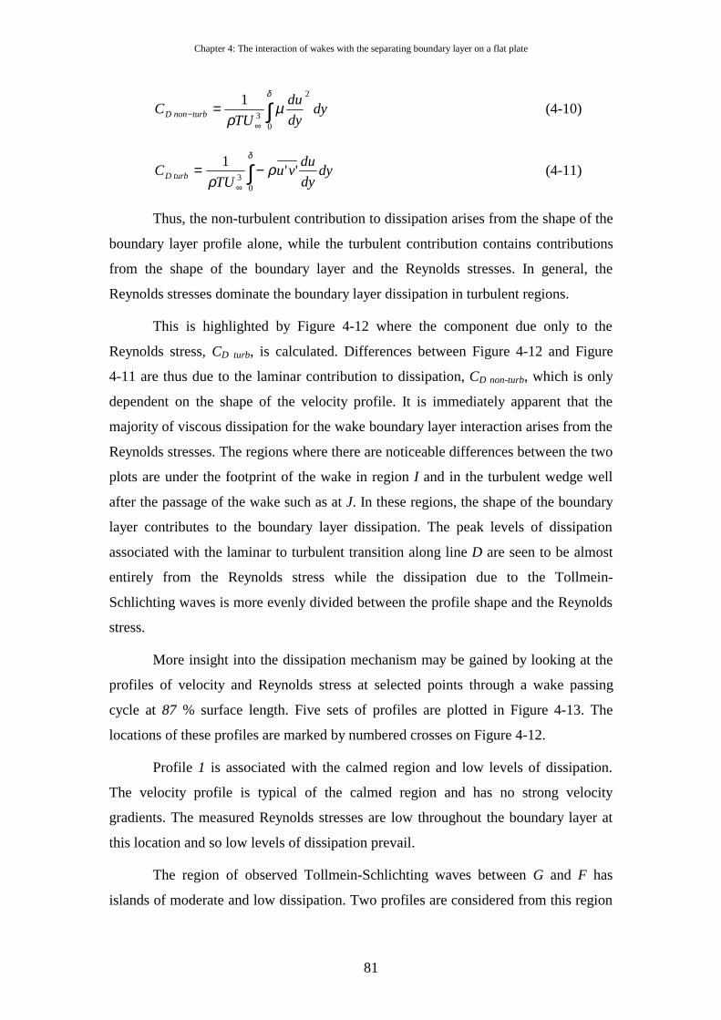
Chapter 4: The interaction of wakes with the separating boundary layer on a flat plate
81
∫∞
− =δ
µρ 0
2
3
1dy
dy
du
TUC turbnonD (4-10)
∫ −=∞
δ
ρρ 0
3''
1dy
dy
duvu
TUC turbD (4-11)
Thus, the non-turbulent contribution to dissipation arises from the shape of the
boundary layer profile alone, while the turbulent contribution contains contributions
from the shape of the boundary layer and the Reynolds stresses. In general, the
Reynolds stresses dominate the boundary layer dissipation in turbulent regions.
This is highlighted by Figure 4-12 where the component due only to the
Reynolds stress, CD turb, is calculated. Differences between Figure 4-12 and Figure
4-11 are thus due to the laminar contribution to dissipation, CD non-turb, which is only
dependent on the shape of the velocity profile. It is immediately apparent that the
majority of viscous dissipation for the wake boundary layer interaction arises from the
Reynolds stresses. The regions where there are noticeable differences between the two
plots are under the footprint of the wake in region I and in the turbulent wedge well
after the passage of the wake such as at J. In these regions, the shape of the boundary
layer contributes to the boundary layer dissipation. The peak levels of dissipation
associated with the laminar to turbulent transition along line D are seen to be almost
entirely from the Reynolds stress while the dissipation due to the Tollmein-
Schlichting waves is more evenly divided between the profile shape and the Reynolds
stress.
More insight into the dissipation mechanism may be gained by looking at the
profiles of velocity and Reynolds stress at selected points through a wake passing
cycle at 87 % surface length. Five sets of profiles are plotted in Figure 4-13. The
locations of these profiles are marked by numbered crosses on Figure 4-12.
Profile 1 is associated with the calmed region and low levels of dissipation.
The velocity profile is typical of the calmed region and has no strong velocity
gradients. The measured Reynolds stresses are low throughout the boundary layer at
this location and so low levels of dissipation prevail.
The region of observed Tollmein-Schlichting waves between G and F has
islands of moderate and low dissipation. Two profiles are considered from this region
Chapter 4: The interaction of wakes with the separating boundary layer on a flat plate
82
to aid the explanation and show the source of the differences. Profile 2 is associated
with higher levels of dissipation than profile 3 yet the velocity profiles are very
similar and inflexional in character. The differences in dissipation result from the
difference in the level of Reynolds stress. Profile 2 has a peak in Reynolds stress at
the mid boundary layer height while 3 has lower levels more uniformly distributed
and confined to the inner half of the boundary layer height.
The peak levels of CD are associated with profile 4 and result from the
laminar to turbulent transition. The boundary layer profile is not yet full like a typical
turbulent profile, nor is it inflexional like profiles 2 and 3. The contribution from the
profile shape is thus minor. The peak values of CD are thus achieved primarily by the
very high levels of Reynolds stress. However, due to the shape of the profile, the
velocity gradients in the region of high Reynolds stress are also higher. Therefore, the
peak levels of CD are achieved through the combined effect of very high Reynolds
stresses, and the relative location of the velocity gradients within the boundary layer.
The profile 5 taken from within the wake induced turbulent wedge is
associated with a high level of CD but with a noticeable non-turbulent contribution.
The velocity profile at this location has a full turbulent shape. The near wall velocity
gradient is thus very high and this accounts for the non-turbulent contribution to CD.
The Reynolds stresses are high throughout the boundary layer height, although in the
outer part of the boundary layer, the velocity gradients are low and thus the
contribution to dissipation is diminished in this region.
4.5.5 Comparison of measured and expected levels of dissipation The general level of dissipation for a turbulent boundary layer is given by
Schlichting (1979) as an experimentally based correlation. For a turbulent boundary
layer with 1.2<H12<2.0 and 103<Reθ<105 the dissipation may be correlated as
6/1Re0056.0 −= θDC ( 4-12)
Denton (1993) shows that a Cebeci boundary layer calculation with a mixing
length turbulence model produces similar results to this correlation for zero pressure
gradient. The same calculation predicts diffusing flows to have elevated dissipation
and accelerating flows to have reduced dissipation. However, these results are simply
a measure of the ability of the mixing length turbulence model to determine boundary
layer dissipation.
Chapter 4: The interaction of wakes with the separating boundary layer on a flat plate
83
In laminar boundary layers, CD is more strongly dependent on the boundary
layer thickness and Truckenbrodt (1952) provides the correlation
1Re −= θβDC ( 4-13)
and an analytic solution for a zero pressure gradient laminar boundary layer gives a
coefficient β=0.173. Denton (1993) suggests accounting for pressure gradients by
considering the Pohlhausen velocity profiles. For a highly accelerated boundary layer
with λ=+12 the coefficient is β=0.220 while for the separating Pohlhausen profile
with λ=-12 the coefficient is β=0.151.
The correlations for turbulent and laminar boundary layers are presented in
Figure 4-14. Also shown on Figure 4-14 are data of the ensemble-averaged
measurements of dissipation and Reθ. Each measured data point is indicated by a
circle and the scatter indicates the range of values measured. The points of highest Reθ
correspond to the wake-induced strip and have levels of CD significantly higher than
predicted by the correlation of Schlichting. The greatest density of measurement
points lie in the range 200< Reθ<300 where the levels of CD are laminar and in
reasonable agreement with the correlation of Truckenbrodt. The time average of the
measured ensemble average Reθs and CD is shown by the heavy line. These values lie
between the expected laminar and turbulent levels from the first measurement point
until Reθ=450 which is at 83 % surface length. Thereafter the levels marginally
exceed the correlation of Schlichting as anticipated in a decelerating flow.
The time average measurements of CD are thus in reasonable agreement with
anticipated levels which credits the validity of the measurements. However, the levels
of CD and Reθ that occur during the wake-induced transition are significantly higher
than anticipated and the correlation of Schlichting, which is based on steady
experimental data, is unable to capture any of the unsteady effects of wake-induced
transition.
4.6 Conclusion from Flat Plate measurements The results presented in this chapter demonstrate that it is possible to simulate
the boundary layers of LP turbine blades on a flat plate by imposing a representative
pressure distribution.

Chapter 4: The interaction of wakes with the separating boundary layer on a flat plate
84
The interaction of a wake and a boundary layer was dominated by the
unsteady wake induced transition phenomena. Wake turbulence resulted in periodic
early bypass transition. This prevented the formation of a steady separation bubble.
The turbulent to laminar relaxation of the boundary layer that occurred between wake
passing events was governed by the calmed region.
A deterministic natural transition mechanism was identified in the boundary
layer as it relaxed from turbulent to laminar between wake passing events. The
frequency of velocity fluctuations observed towards the trailing edge was found to be
in good agreement with the frequency predicted from the most amplified Tollmein-
Schlichting waves in a Falkner-Skan profile of the same displacement thickness.
Ensemble averaged measurements of velocity profiles and Reynolds stress
profiles along the surface of the flat plate facilitated the calculation of the boundary
layer dissipation coefficient. Experimental proof of the loss reducing mechanism
associated with the calmed region following the wake induced turbulent boundary
layer was thus provided.
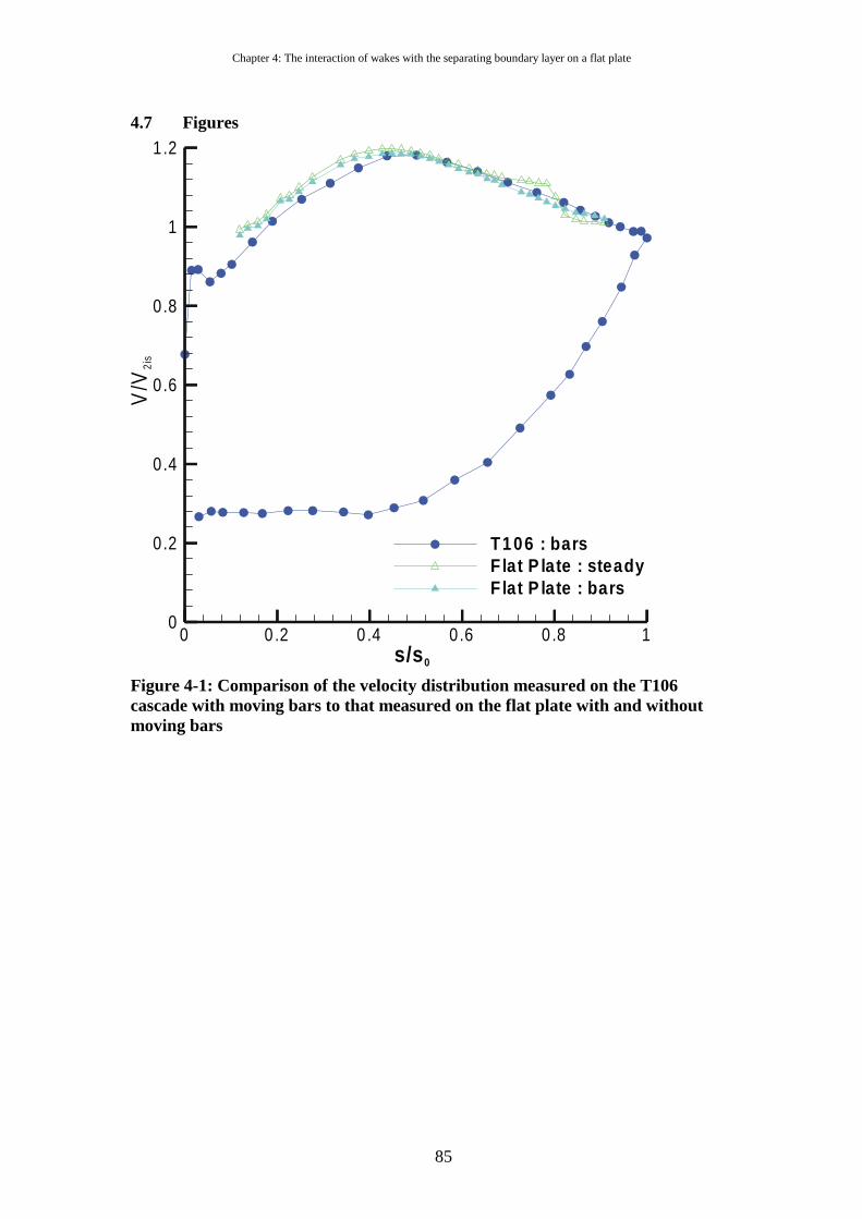
Chapter 4: The interaction of wakes with the separating boundary layer on a flat plate
85
4.7 Figures
0 0 .2 0 .4 0.6 0 .8 1s/s 0
0
0.2
0.4
0.6
0.8
1
1.2
T1 06 : barsF lat P late : steadyF lat P late : bars
V/V
2is
Figure 4-1: Comparison of the velocity distribution measured on the T106 cascade with moving bars to that measured on the flat plate with and without moving bars
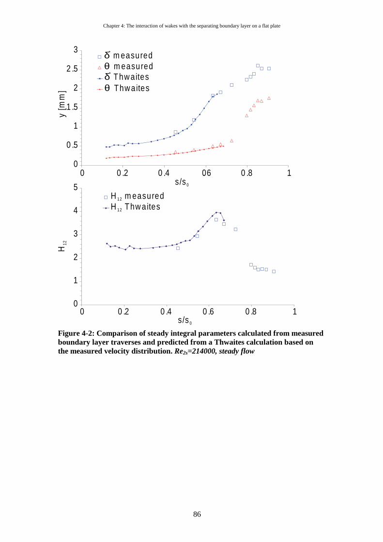
Chapter 4: The interaction of wakes with the separating boundary layer on a flat plate
86
0
0 .5
1
1 .5
2
2 .5
3
0 0 .2 0 .4 0. 6 0 .8 1s/s0
δ∗ m easured
θ m easured δ∗ Thw aites
θ Thw aites
0
1
2
3
4
5
0 0 .2 0 .4 0 .6 0 .8 1s/s 0
H m easured12
H Thw aites12
y [m
m]
H12
Figure 4-2: Comparison of steady integral parameters calculated from measured boundary layer traverses and predicted from a Thwaites calculation based on the measured velocity distribution. Re2s=214000, steady flow
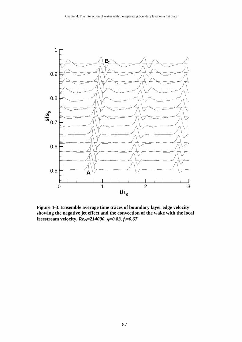
Chapter 4: The interaction of wakes with the separating boundary layer on a flat plate
87
t/τ0
s/s 0
0 1 2 3
0.5
0.6
0.7
0.8
0.9
1
A
B
Figure 4-3: Ensemble average time traces of boundary layer edge velocity showing the negative jet effect and the convection of the wake with the local freestream velocity. Re2s=214000, φ=0.83, fr=0.67
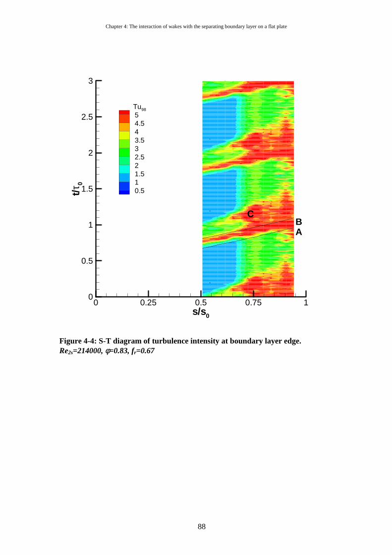
Chapter 4: The interaction of wakes with the separating boundary layer on a flat plate
88
AB
C
s/s0
t/τ0
0 0.25 0.5 0.75 10
0.5
1
1.5
2
2.5
3
Tu98
54.543.532.521.510.5
Figure 4-4: S-T diagram of turbulence intensity at boundary layer edge. Re2s=214000, φ=0.83, fr=0.67
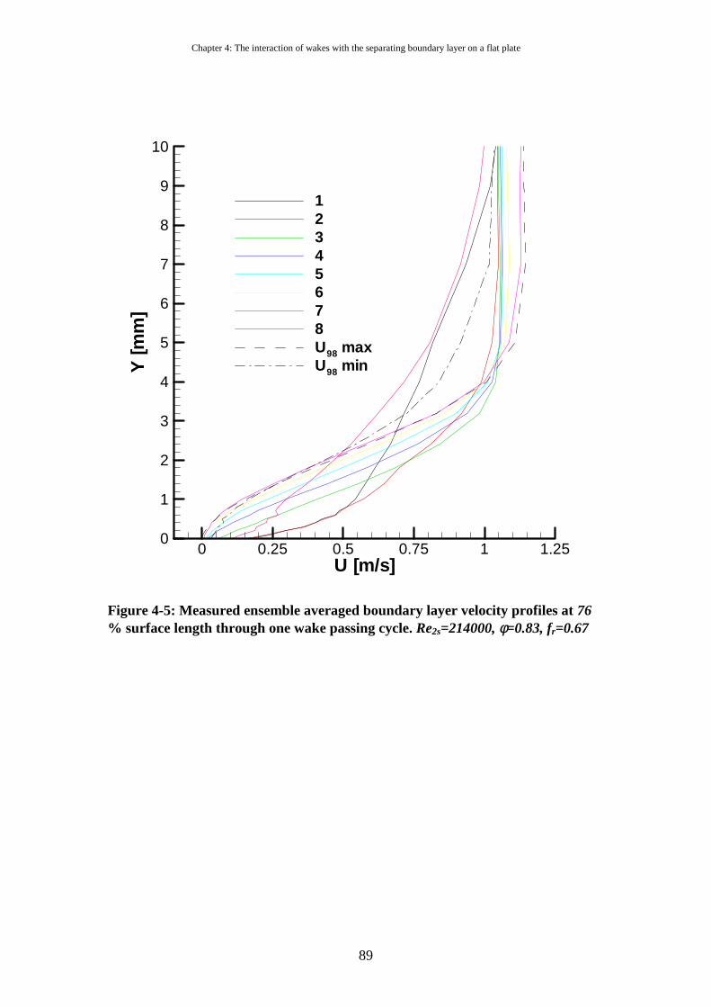
Chapter 4: The interaction of wakes with the separating boundary layer on a flat plate
89
U [m/s]
Y[m
m]
0 0.25 0.5 0.75 1 1.250
1
2
3
4
5
6
7
8
9
10
12345678U98 maxU98 min
Figure 4-5: Measured ensemble averaged boundary layer velocity profiles at 76 % surface length through one wake passing cycle. Re2s=214000, φ=0.83, fr=0.67
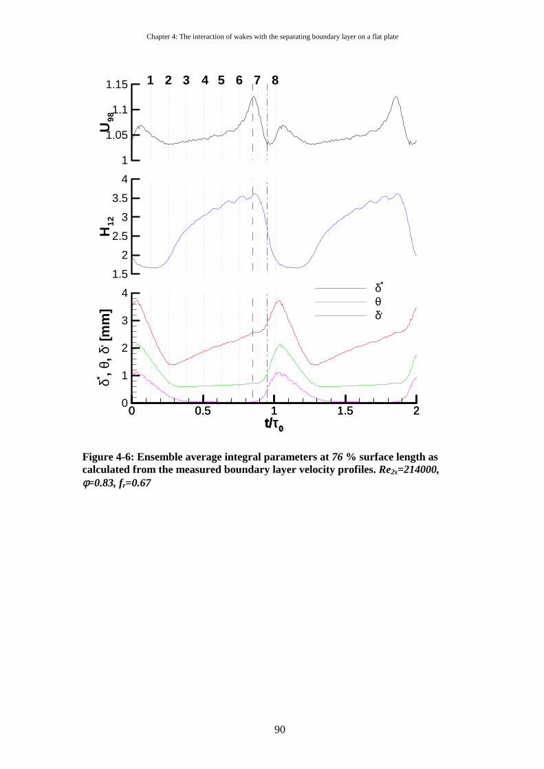
Chapter 4: The interaction of wakes with the separating boundary layer on a flat plate
90
t/τ0
H1
2
0 0.5 1 1.5 2
1.5
2
2.5
3
3.5
4
t/τ0
U98
0 0.5 1 1.5 2
1
1.05
1.1
1.15
t/τ0
δ* ,θ,δ
,[m
m]
0 0.5 1 1.5 20
1
2
3
4 δ*
θδ,
1 2 3 4 5 6 7 8
Figure 4-6: Ensemble average integral parameters at 76 % surface length as calculated from the measured boundary layer velocity profiles. Re2s=214000, φ=0.83, fr=0.67
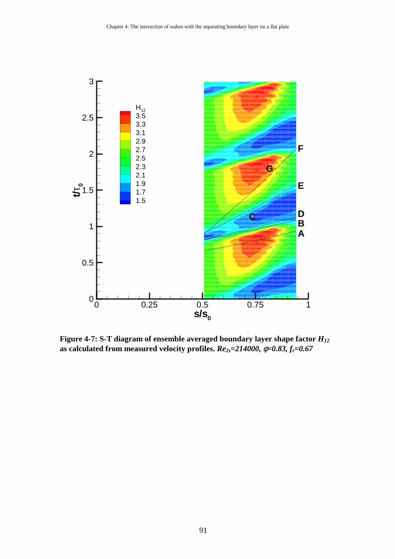
Chapter 4: The interaction of wakes with the separating boundary layer on a flat plate
91
AB
C D
E
F
G
s/s0
t/τ0
0 0.25 0.5 0.75 10
0.5
1
1.5
2
2.5
3
H12
3.53.33.12.92.72.52.32.11.91.71.5
Figure 4-7: S-T diagram of ensemble averaged boundary layer shape factor H12 as calculated from measured velocity profiles. Re2s=214000, φ=0.83, fr=0.67
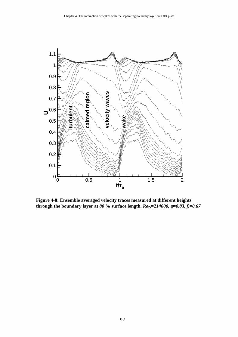
Chapter 4: The interaction of wakes with the separating boundary layer on a flat plate
92
t/τ0
U
0 0.5 1 1.5 20
0.1
0.2
0.3
0.4
0.5
0.6
0.7
0.8
0.9
1
1.1
wak
e
turb
ulen
t
calm
edre
gion
velo
city
wav
es
Figure 4-8: Ensemble averaged velocity traces measured at different heights through the boundary layer at 80 % surface length. Re2s=214000, φ=0.83, fr=0.67
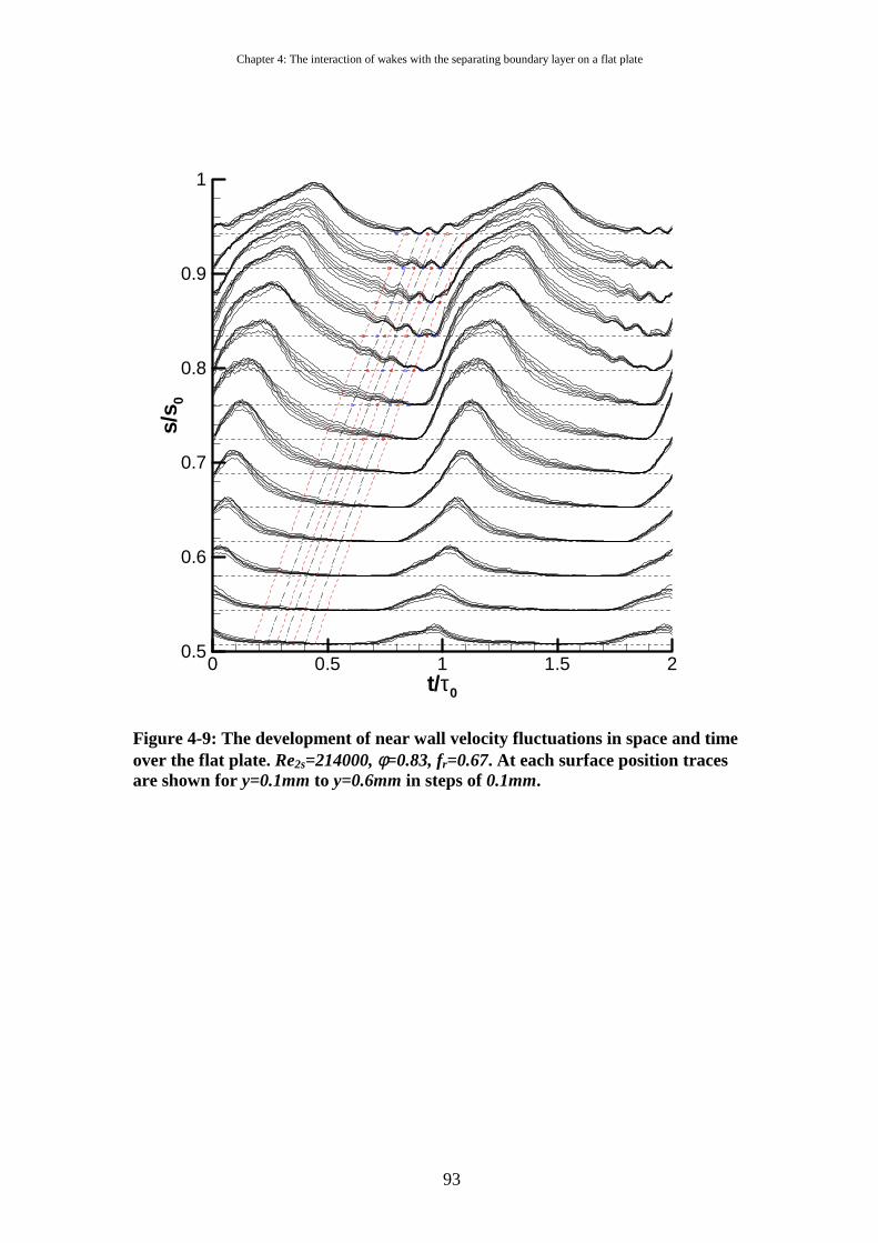
Chapter 4: The interaction of wakes with the separating boundary layer on a flat plate
93
t/τ0
s/s 0
0 0.5 1 1.5 20.5
0.6
0.7
0.8
0.9
1
Figure 4-9: The development of near wall velocity fluctuations in space and time over the flat plate. Re2s=214000, φ=0.83, fr=0.67. At each surface position traces are shown for y=0.1mm to y=0.6mm in steps of 0.1mm.
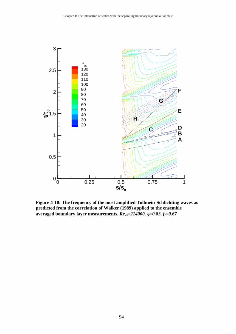
Chapter 4: The interaction of wakes with the separating boundary layer on a flat plate
94
AB
C D
E
F
G
H
s/s0
t/τ0
0 0.25 0.5 0.75 10
0.5
1
1.5
2
2.5
3
fTS
1301201101009080706050403020
Figure 4-10: The frequency of the most amplified Tollmein-Schlichting waves as predicted from the correlation of Walker (1989) applied to the ensemble averaged boundary layer measurements. Re2s=214000, φ=0.83, fr=0.67
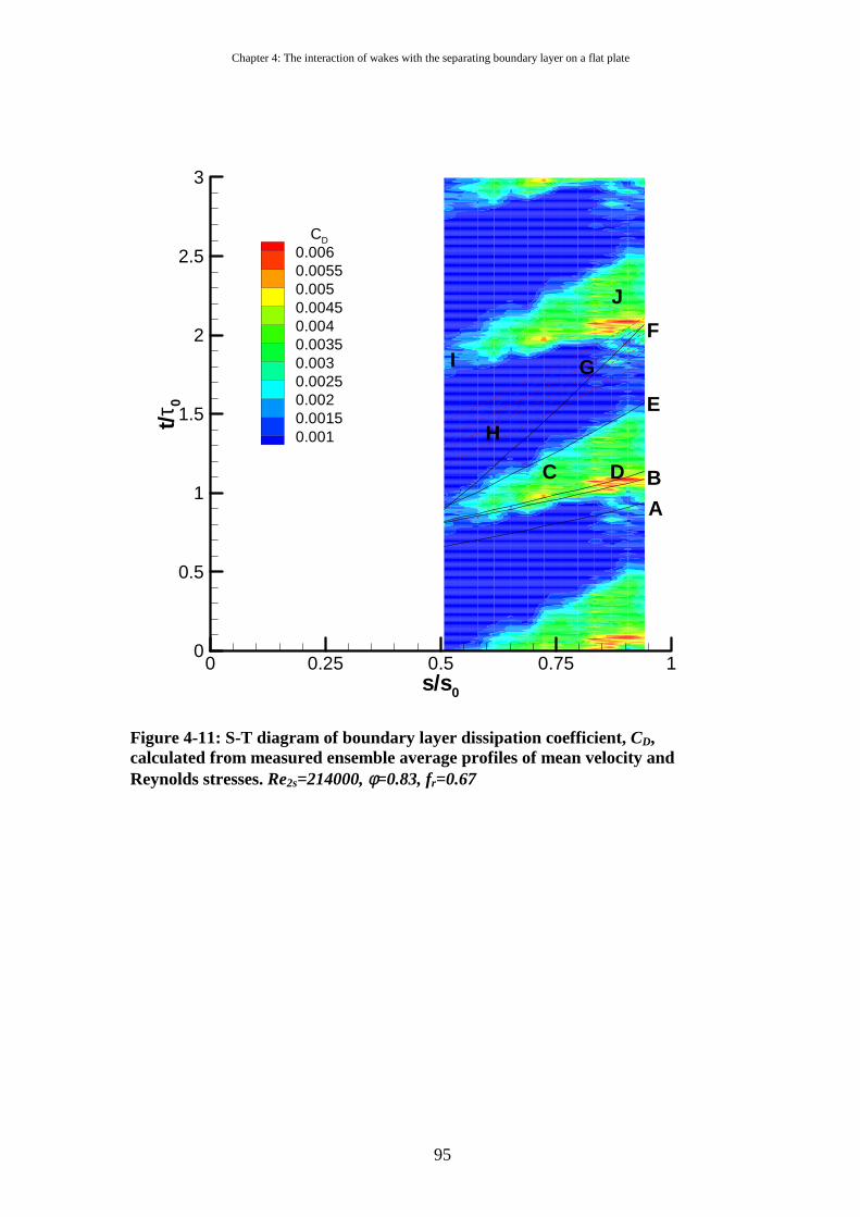
Chapter 4: The interaction of wakes with the separating boundary layer on a flat plate
95
A
BC D
E
I G
H
J
F
s/s0
t/τ0
0 0.25 0.5 0.75 10
0.5
1
1.5
2
2.5
3
CD
0.0060.00550.0050.00450.0040.00350.0030.00250.0020.00150.001
Figure 4-11: S-T diagram of boundary layer dissipation coefficient, CD, calculated from measured ensemble average profiles of mean velocity and Reynolds stresses. Re2s=214000, φ=0.83, fr=0.67
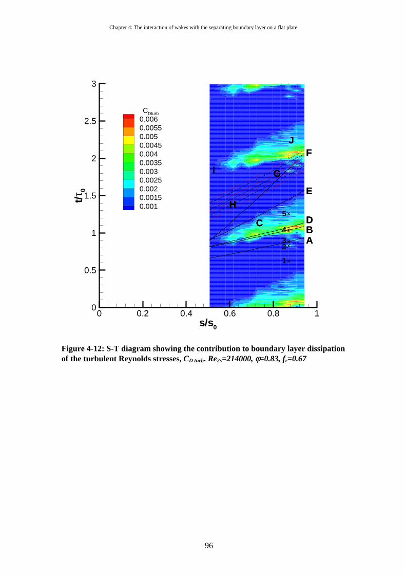
Chapter 4: The interaction of wakes with the separating boundary layer on a flat plate
96
C
E
G
H
DB
FJ
I
x
xx
x
x
A
1
234
5
A
C
E
F
G
H
DB
s/s0
t/τ0
0 0.2 0.4 0.6 0.8 10
0.5
1
1.5
2
2.5
3
CDturb
0.0060.00550.0050.00450.0040.00350.0030.00250.0020.00150.001
Figure 4-12: S-T diagram showing the contribution to boundary layer dissipation of the turbulent Reynolds stresses, CD turb. Re2s=214000, φ=0.83, fr=0.67
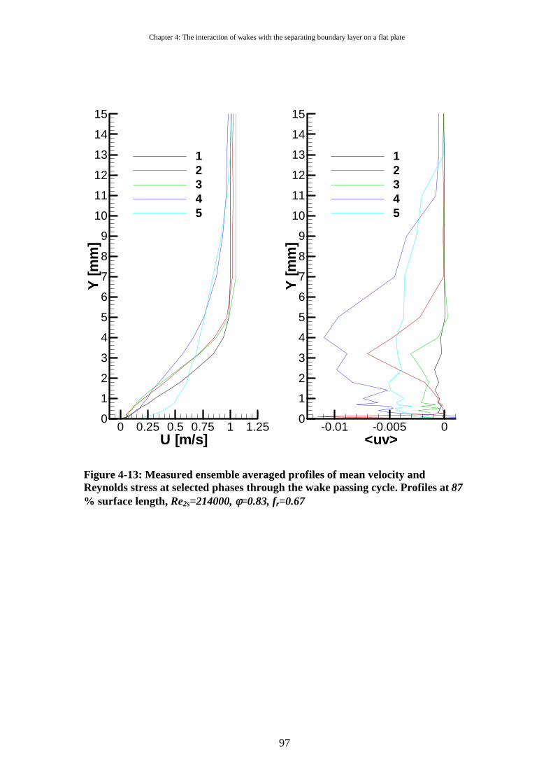
Chapter 4: The interaction of wakes with the separating boundary layer on a flat plate
97
U [m/s]
Y[m
m]
0 0.25 0.5 0.75 1 1.250
1
2
3
4
5
6
7
8
9
10
11
12
13
14
15
12345
<uv>
Y[m
m]
-0.01 -0.005 00
1
2
3
4
5
6
7
8
9
10
11
12
13
14
15
12345
Figure 4-13: Measured ensemble averaged profiles of mean velocity and Reynolds stress at selected phases through the wake passing cycle. Profiles at 87 % surface length, Re2s=214000, φ=0.83, fr=0.67
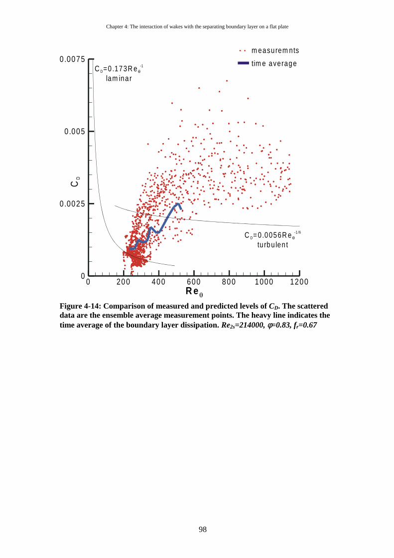
Chapter 4: The interaction of wakes with the separating boundary layer on a flat plate
98
0 200 400 600 800 1000 1200R eθ
0
0 .0025
0.005
0 .0075C =0.173R e
lam inarD θ
-1
C =0.0056R eturbu len t
D θ-1 /6
tim e average
m easurem nts
CD
Figure 4-14: Comparison of measured and predicted levels of CD. The scattered data are the ensemble average measurement points. The heavy line indicates the time average of the boundary layer dissipation. Re2s=214000, φ=0.83, fr=0.67
99
Chapter 5: Measurement of turbulent wake convection through an axial turbine cascade
5.1 Introduction The unsteady flow field in LP turbines is governed by a combination of
potential and convective interactions (Hodson, 1998). Of these, the convected wakes
from upstream blade rows play the most significant role due to their effect upon the
blade surface boundary layers.
A number of researchers have described the kinematics governing the
convection of a wake through a cascade. Early work by Meyer (1958) used potential
flow solutions and resulted in the negative jet model. Numerous numerical studies
have further shown that the wake convection is primarily a kinematic phenomenon
(e.g. Hodson, 1985 and Giles, 1987).
However, the kinematics of the wake convection is only partly responsible for
the effects of the wake on the blade surface boundary layer. The primary effect of the
wake convection is to dictate boundary layer transition and so it is the turbulence of
the wake and the convection of the turbulent quantities through the blade row that is
of prime importance. Indeed, the transition models of Addison and Hodson (1992),
Doorly and Oldfield (1985) and La Graff et al (1989) all neglect the negative jet
effect. These models use the wake convection simply to transport wake turbulence,
which acts as a transition onset front.
To date, few measurements exist of the unsteady wake convection through a
turbine blade row. The measurements of Schulte (1995) provide a guide to the mean
flow through a LP turbine passage, however these measurements lack resolution and
detail of the turbulent quantities.
This chapter presents 2D LDA measurements of the wake convection through
the T106 LP turbine cascade. Not only is the spatial resolution of the measurements
unprecedented but also the direct measurement of Reynolds stresses provides a
valuable database for comparison of numerical predictions. Based on the measured
mean and turbulent quantities, the production of turbulent kinetic energy is calculated.
A novel wavelet analysis of the 2D LDA data is also presented at representative
points within the blade passage. This provides understanding of the contributions of
the different scales to the turbulent quantities during the wake passing cycle.
Chapter 5: Measurement of turbulent wake convection through an axial turbine cascade
100
The measured ensemble-averaged velocity field confirmed the previously
reported kinematics of wake convection. Measurements of the turbulent quantities
showed the wake fluid to be characterised by elevated levels of turbulent kinetic
energy (TKE) and to have an anisotropic structure. Production of TKE within the
blade passage elevated the TKE levels and resulted in a more isotropic turbulent flow
above the suction surface at about mid-chord.
5.2 Measurement details The convection of wakes shed from a moving bar wake generator through the
T106 LP turbine cascade was measured using 2D LDA as described in Chapter 3. The
measurement grid consisted of 35 tangential traverses evenly spaced in the axial
direction within the bladerow. A further 4 traverses were performed upstream of the
leading edge of the cascade. Each tangential traverse consisted of 48 points. The beam
pairs of the LDA intersect at a half angle of 4.3° so in order to make measurements
close to the blade surfaces it was necessary to incline the probe so that neither of the
beams was obstructed by the blade. The traverses in the axial planes were thus
performed in two stages with 24 points equally spaced from the suction surface and
then, after altering the probe inclination, 24 equally spaced from the pressure surface.
The suction side traverses were performed at a marginally smaller spacing than those
from the pressure side. The velocity measured with the inclined LDA probe is
insignificantly different from that measured with a normal probe (less than 0.5%) and
for this reason it was considered unnecessary to apply a correction to the
measurements.
The blade surface was painted matt black to minimise flare from the
intersecting beams. However, a narrow strip at mid span was left unpainted to avoid
contaminating the mid-span static pressure tappings. For this reason all measurements
were performed at 45% span. The measurement grid with the blades and bars
superimposed together with the definitions of the co-ordinate directions and velocity
components is shown in Figure 5-1.
A trigger signal was supplied on every bar passing and was used to ensemble
average the LDA data using the methods described in Chapter 3. Each bar passing
cycle was divided into 128 time bins, which provided adequate temporal resolution of
the ensemble averaged flow physics.
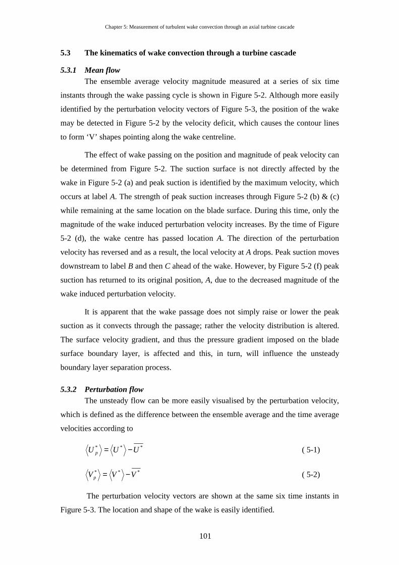
Chapter 5: Measurement of turbulent wake convection through an axial turbine cascade
101
5.3 The kinematics of wake convection through a turbine cascade
5.3.1 Mean flow The ensemble average velocity magnitude measured at a series of six time
instants through the wake passing cycle is shown in Figure 5-2. Although more easily
identified by the perturbation velocity vectors of Figure 5-3, the position of the wake
may be detected in Figure 5-2 by the velocity deficit, which causes the contour lines
to form ‘V’ shapes pointing along the wake centreline.
The effect of wake passing on the position and magnitude of peak velocity can
be determined from Figure 5-2. The suction surface is not directly affected by the
wake in Figure 5-2 (a) and peak suction is identified by the maximum velocity, which
occurs at label A. The strength of peak suction increases through Figure 5-2 (b) & (c)
while remaining at the same location on the blade surface. During this time, only the
magnitude of the wake induced perturbation velocity increases. By the time of Figure
5-2 (d), the wake centre has passed location A. The direction of the perturbation
velocity has reversed and as a result, the local velocity at A drops. Peak suction moves
downstream to label B and then C ahead of the wake. However, by Figure 5-2 (f) peak
suction has returned to its original position, A, due to the decreased magnitude of the
wake induced perturbation velocity.
It is apparent that the wake passage does not simply raise or lower the peak
suction as it convects through the passage; rather the velocity distribution is altered.
The surface velocity gradient, and thus the pressure gradient imposed on the blade
surface boundary layer, is affected and this, in turn, will influence the unsteady
boundary layer separation process.
5.3.2 Perturbation flow The unsteady flow can be more easily visualised by the perturbation velocity,
which is defined as the difference between the ensemble average and the time average
velocities according to
*** UUU p −= ( 5-1)
*** VVVp −= ( 5-2)
The perturbation velocity vectors are shown at the same six time instants in
Figure 5-3. The location and shape of the wake is easily identified.
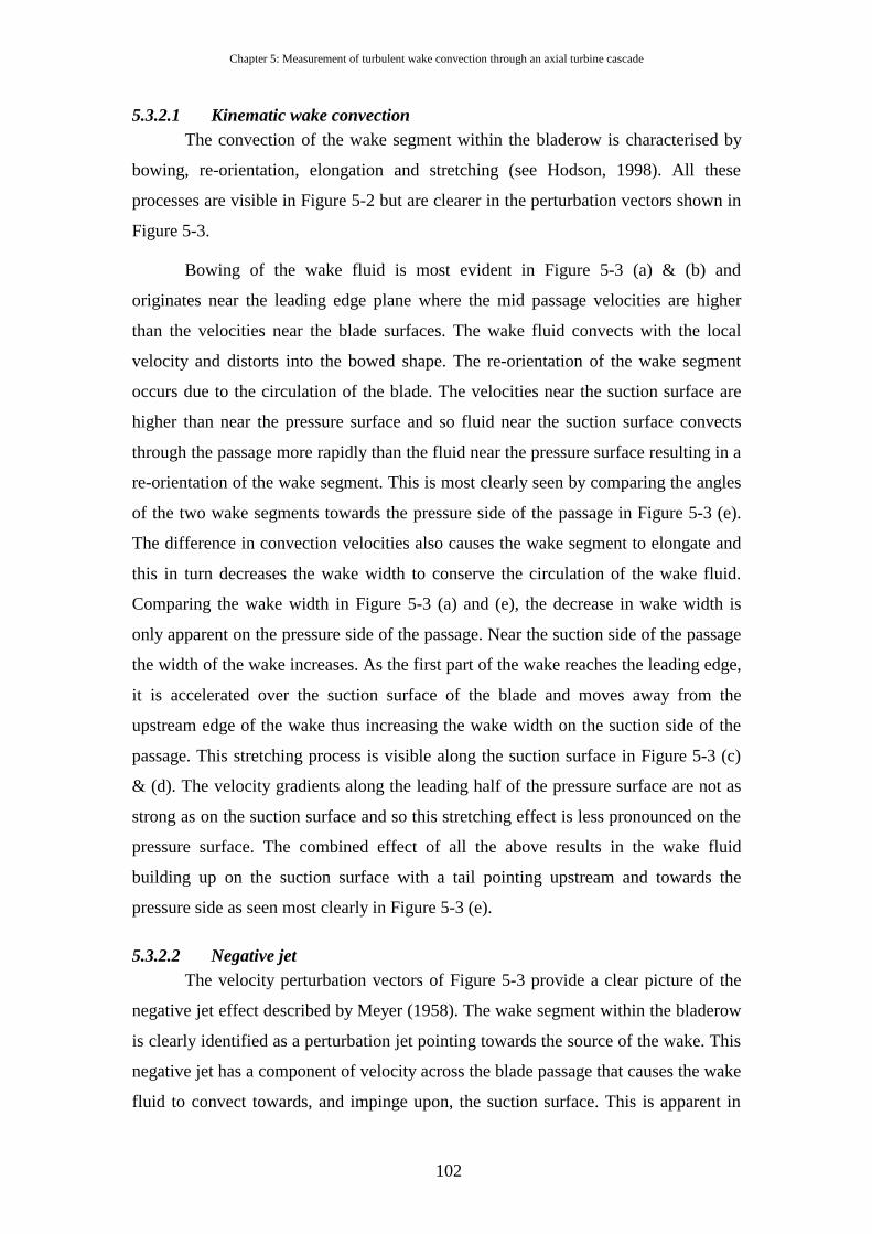
Chapter 5: Measurement of turbulent wake convection through an axial turbine cascade
102
5.3.2.1 Kinematic wake convection The convection of the wake segment within the bladerow is characterised by
bowing, re-orientation, elongation and stretching (see Hodson, 1998). All these
processes are visible in Figure 5-2 but are clearer in the perturbation vectors shown in
Figure 5-3.
Bowing of the wake fluid is most evident in Figure 5-3 (a) & (b) and
originates near the leading edge plane where the mid passage velocities are higher
than the velocities near the blade surfaces. The wake fluid convects with the local
velocity and distorts into the bowed shape. The re-orientation of the wake segment
occurs due to the circulation of the blade. The velocities near the suction surface are
higher than near the pressure surface and so fluid near the suction surface convects
through the passage more rapidly than the fluid near the pressure surface resulting in a
re-orientation of the wake segment. This is most clearly seen by comparing the angles
of the two wake segments towards the pressure side of the passage in Figure 5-3 (e).
The difference in convection velocities also causes the wake segment to elongate and
this in turn decreases the wake width to conserve the circulation of the wake fluid.
Comparing the wake width in Figure 5-3 (a) and (e), the decrease in wake width is
only apparent on the pressure side of the passage. Near the suction side of the passage
the width of the wake increases. As the first part of the wake reaches the leading edge,
it is accelerated over the suction surface of the blade and moves away from the
upstream edge of the wake thus increasing the wake width on the suction side of the
passage. This stretching process is visible along the suction surface in Figure 5-3 (c)
& (d). The velocity gradients along the leading half of the pressure surface are not as
strong as on the suction surface and so this stretching effect is less pronounced on the
pressure surface. The combined effect of all the above results in the wake fluid
building up on the suction surface with a tail pointing upstream and towards the
pressure side as seen most clearly in Figure 5-3 (e).
5.3.2.2 Negative jet The velocity perturbation vectors of Figure 5-3 provide a clear picture of the
negative jet effect described by Meyer (1958). The wake segment within the bladerow
is clearly identified as a perturbation jet pointing towards the source of the wake. This
negative jet has a component of velocity across the blade passage that causes the wake
fluid to convect towards, and impinge upon, the suction surface. This is apparent in

Chapter 5: Measurement of turbulent wake convection through an axial turbine cascade
103
Figure 5-3 (d)-(f). As the wake fluid impinges on the surface, it splits into two
perturbation streams, one pointed downstream along the blade and the other upstream
along the blade. Thus, downstream of the wake centre the perturbation from the
negative jet is in the same direction as the main flow, while upstream of the wake
centre it opposes the mean flow.
5.3.2.3 Vorticity The negative jet, trapped between two solid blades, establishes a pair of
counter rotating vortices. These counter rotating vortices, with centres marked ‘D’
and ‘E’ in Figure 5-3 (c) - (f), are clearly visible in the perturbation velocity vector
plots as they convect through the blade passage.
The flow area reduces as the flow accelerates through the bladerow.
According to Kelvin’s theorem, the vorticity must therefore increase to conserve
angular momentum. Evidence of this is seen by the increase in the magnitude of the
perturbation vectors through the blade passage. The vortex pair also convects towards
the suction surface under the influence of the cross passage transport. The interaction
of the vortex pair with the blade surface may be explained by considering an
imaginary image system to be formed through the blade surface. As the suction
surface is approached, the interaction of the vortex pair with the image system causes
the separation between the vortex centres to increase and further magnifies the
perturbation velocity magnitude.
Figure 5-4 presents contours of non-dimensional vorticity, Ω*, calculated as
*
*
*
*
*
y
U
x
V
∂
∂−
∂
∂=Ω ( 5-3)
where the derivatives were determined using Green’s theorem as described in
Appendix IV. The position and shape of the wake is again evident from the shear
layers either side of the wake centre. It is apparent that the wake velocity distribution
can be represented by a vorticity distribution as suggested by Smith (1966). The
counter rotating vortex pair is evident in the build-up of vorticity at mid pitch. As the
wake reaches the rear portion of the blade passage (Figure 5-4 (d)-(f)), the
unsteadiness of the flow increases the random error of the measured velocities, which
are amplified in the calculation of vorticity. Along the forward region of the suction
surface and along the pressure surface the wake centre line is stretched. The stretching
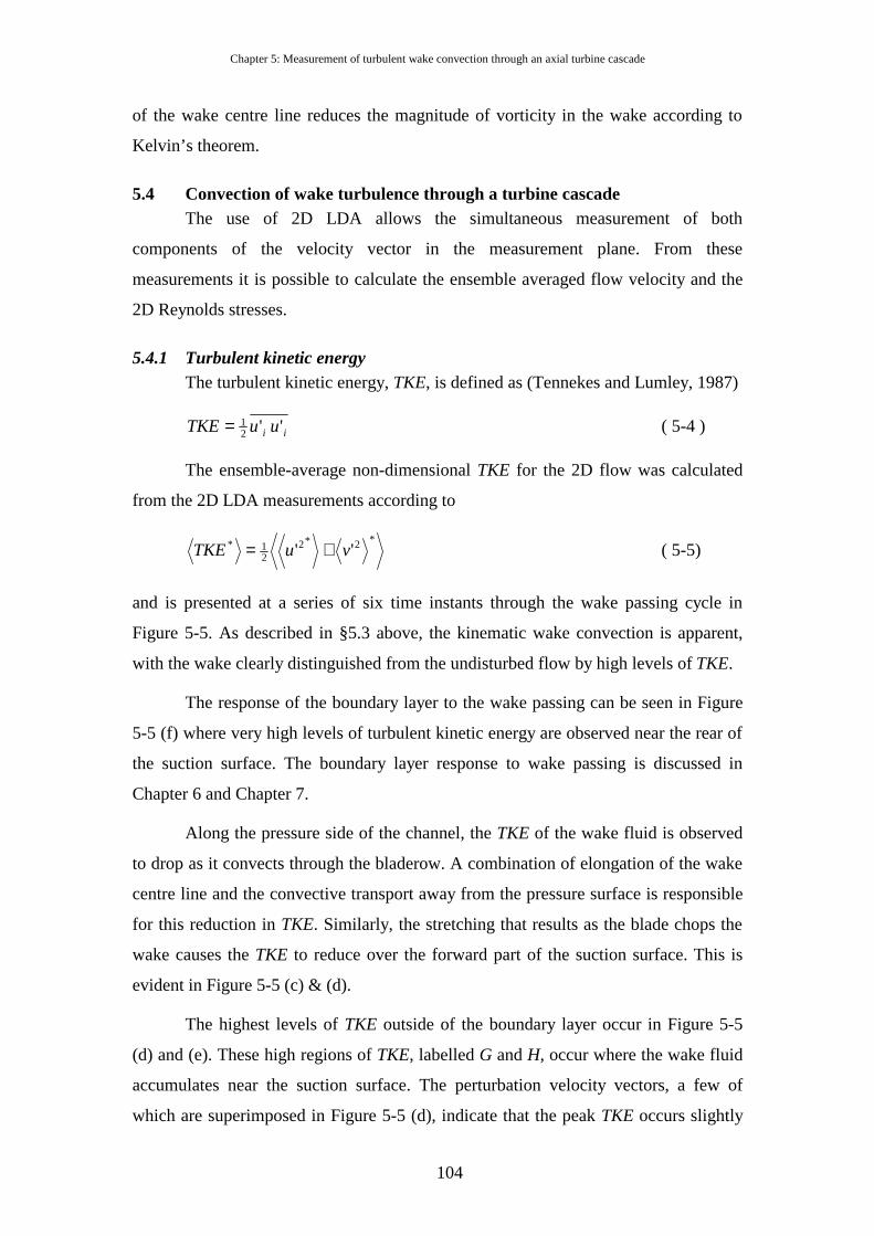
Chapter 5: Measurement of turbulent wake convection through an axial turbine cascade
104
of the wake centre line reduces the magnitude of vorticity in the wake according to
Kelvin’s theorem.
5.4 Convection of wake turbulence through a turbine cascade The use of 2D LDA allows the simultaneous measurement of both
components of the velocity vector in the measurement plane. From these
measurements it is possible to calculate the ensemble averaged flow velocity and the
2D Reynolds stresses.
5.4.1 Turbulent kinetic energy The turbulent kinetic energy, TKE, is defined as (Tennekes and Lumley, 1987)
ii uuTKE ''21= ( 5-4 )
The ensemble-average non-dimensional TKE for the 2D flow was calculated
from the 2D LDA measurements according to
*2*221* '' vuTKE += ( 5-5)
and is presented at a series of six time instants through the wake passing cycle in
Figure 5-5. As described in §5.3 above, the kinematic wake convection is apparent,
with the wake clearly distinguished from the undisturbed flow by high levels of TKE.
The response of the boundary layer to the wake passing can be seen in Figure
5-5 (f) where very high levels of turbulent kinetic energy are observed near the rear of
the suction surface. The boundary layer response to wake passing is discussed in
Chapter 6 and Chapter 7.
Along the pressure side of the channel, the TKE of the wake fluid is observed
to drop as it convects through the bladerow. A combination of elongation of the wake
centre line and the convective transport away from the pressure surface is responsible
for this reduction in TKE. Similarly, the stretching that results as the blade chops the
wake causes the TKE to reduce over the forward part of the suction surface. This is
evident in Figure 5-5 (c) & (d).
The highest levels of TKE outside of the boundary layer occur in Figure 5-5
(d) and (e). These high regions of TKE, labelled G and H, occur where the wake fluid
accumulates near the suction surface. The perturbation velocity vectors, a few of
which are superimposed in Figure 5-5 (d), indicate that the peak TKE occurs slightly

Chapter 5: Measurement of turbulent wake convection through an axial turbine cascade
105
below the centres of the counter rotating vortex pair. The elevated TKE does not
penetrate to the boundary layer. In this region the turbulence intensity based on
isentropic exit velocity is Tu=7% where the wake centreline turbulence intensity at
the leading edge plane is Tu=5%. The increase in the level of TKE is seen to begin in
Figure 5-5 (c) at label F and continue through Figure 5-5 (d)-(f), although it is the
extent and not the level that increases between G and H.
The production of TKE, PTKE, is given by Tennekes and Lumley (1987) as
j
ijiTKE x
UuuP
∂∂
−= '' ( 5-6 )
The measured ensemble averaged Reynolds stresses were used together with the
ensemble average velocity derivatives calculated from Green’s theorem, as described
in Appendix IV, to evaluate the ensemble averaged non-dimensional production of
TKE in the blade-to-blade plane according to
∂
∂+
∂
∂−
∂
∂−
∂
∂−=
*
*
*
*
**
**2
*
**2* ''''
x
V
y
Uvu
y
Vv
x
UuPTKE ( 5-7)
The results are presented in Figure 5-6 with the labels copied from Figure 5-5. It is
apparent that the increased levels of TKE are a direct result of TKE production. The
highest production levels occur at labels F and G in Figure 5-6 (c) & (d) and it is these
regions of high production that subsequently lead to regions of high TKE at G and H.
The production of TKE occurs when the turbulence extracts work from the
mean flow and this occurs in regions having high turbulent stresses and high spatial
velocity gradients. The turbulent stresses are confined to the wake fluid and so
production occurs when the wake fluid enters regions of high spatial velocity
gradients. However, it is not only the magnitudes, but also the directions that are
important. If the turbulent stresses and velocity gradients are aligned, the turbulent
production is enhanced.
Throughout the wake passing cycle, it is apparent that the production of TKE
occurs in the wake fluid. This is due to the coexistence of turbulent stresses and the
wake shear layers. Very high levels of TKE production are measured in the boundary
layers on the rear part of the suction surface. This is considered in Chapter 7.

Chapter 5: Measurement of turbulent wake convection through an axial turbine cascade
106
5.4.2 Anisotropy An isotropic turbulent flow is one having the same characteristics of
turbulence in all directions. For any turbulent flow, it is possible to define the
principal stress direction, ψ, as that orientation having zero shear stress according to
−= −
*2*2
*
121
''
''2tan
vu
vuψ ( 5-8)
The principal normal stresses may then be found by a co-ordinate transformation to
align the measured turbulent quantities to the calculated principal directions
)sin(')cos(''*2*2*2 ψψψ ⋅−⋅= vuu ( 5-9)
)cos(')sin(''*2*2*2 ψψψ ⋅−⋅= vuv ( 5-10)
A measure of the anisotropy, α, may then be inferred by taking the modulus of the
ratio of these principal turbulent stresses
*2*2
*2
*2
*2*2
*2
*2
'''
'
'''
'
ψψ
ψ
ψ
ψψ
ψ
ψα
uvifu
v
vuifv
u
>=
>=
( 5-11)
so that the ratio is greater than unity with a value of unity indicating isotropy
Figure 5-7 shows contours of α and it is apparent that the wake fluid is
anisotropic while the undisturbed fluid is essentially isotropic with low turbulent
stresses magnitudes. As the wake fluid reaches the point of peak TKE production,
identified by label ‘F’ in Figure 5-6 (c), the level of anisotropy of the wake fluid falls.
This drop in anisotropy continues and by Figure 5-7 (e), the wake fluid, identified as
having high TKE at label ‘H’ in Figure 5-5 (e), is seen to be essentially isotropic in the
measurement plane14. The TKE production described in §5.4.1 thus results in isotropic
turbulence. The wake fluid near the pressure surface can also be seen to become 14 Strictly speaking, isotropy can only be inferred once the out of plane component of the Reynolds stress is known. The 2D LDA measurements do not provide any information about the third component and the reference to isotropy is purely in a two-dimensional sense.
Chapter 5: Measurement of turbulent wake convection through an axial turbine cascade
107
isotropic as it convects through the bladerow. This is the same region identified as
having low TKE due to stretching of the wake centre line in Figure 5-5.
A possible reason for the high production regions labelled F and G arises due
to the change in flow direction through the bladerow. The turbulent stresses in the
wake are oriented along the wake centreline. As the main flow is turned in the
bladerow, the velocity gradients and turbulent stresses align thereby enhancing the
production of TKE. It is proposed that the turbulent stresses in the wake do not
orientate themselves to the mean flow instantaneously and TKE production may occur
in the bladerow as a result.
5.5 Ensemble average wavelet analysis of LDA data The wavelet transform provides a time–frequency decomposition of a signal
and is thus able to provide information about the scales of turbulence in an unsteady
flow. However, wavelet analysis is traditionally applied to evenly sampled data using
FFT techniques to reduce the computational time. Moreover, for fine scale resolution
high data rates are required. For these reasons, LDA data is not generally suited to
wavelet analysis. However, at certain locations in the current data set the mean data
rate was sufficient to permit a continuous wavelet analysis of limited frequency
resolution.
The wavelet analysis was conducted using a novel adaptation of traditional
wavelet algorithms as described in Appendix III. The discrete Fourier transform of the
unevenly sampled data was calculated directly rather than using traditional FFT
techniques. The convolution of the data and the analysing wavelet was performed in
the frequency domain by taking the product of the discrete Fourier transform and
analysing wavelet. Finally, due to careful selection of the number of frequencies at
which the discrete Fourier transform was calculated, it was possible to obtain the
wavelet transform as the inverse FFT of this product. The wavelet transforms were
ensemble averaged.
The discrete Fourier transform required for the wavelet transform was
calculated at N=128 frequencies per wake passing. This was the maximum resolution
that was permitted by the available data. To ensure that adequate data was present in
each wake passing cycle, the wavelet transform was only counted in the ensemble
average if there were more than NL=128 LDA samples in the ensemble (i.e. NL > N).
Chapter 5: Measurement of turbulent wake convection through an axial turbine cascade
108
The complex valued Morlet wavelet, defined as
2/4/10
20)( ηηωπηϕ −−= eei ( 5-12)
and shown in Figure 5-8 was used for the wavelet analysis. This wavelet was selected
due to its resemblance to a travelling wave packet such as those measured in Chapter
4. The value ω0=6.0 was selected to approximate admissibility (see Farge (1992)).
Following Torrence and Compo (1998), the smallest scale was taken as 1/64 of the
wake passing cycle and the scale resolution was chosen as δj=0.125 thus providing 48
wavelet scales.
5.5.1 Ensemble average wavelet description of Reynolds stresses The wavelet analysis was performed at three locations as shown in Figure 5-1.
Point I is representative of the flow in which the wake has not been significantly
distorted, while J is located at the point where peak TKE production levels were
observed in Figure 5-6 (c). Finally, point K is representative of the high turbulence
flow over the rear of the suction surface, which results from the production of
isotropic turbulence at locations such as J.
Due to the change in the mean flow direction through the turbine passage, the
velocities at each location were aligned to the local time average flow direction before
performing the wavelet transforms. This allows comparison of the streamwise and
cross-stream velocity components at the different locations. The streamwise velocity
component is referred to with subscript 1, while the cross-stream component is
referred to with subscript 2. The shear stress component is referred to with mixed
subscripts.
Following Volino (1998) the wavelet transforms of the Reynolds stresses were
calculated from the wavelet transforms of the velocity components according to
•
•
•
⋅=
⋅=
⋅=
)'()'()''(
)'()'()'(
)'()'()'(
*2
*1
*21
*2
*2
*22
*1
*1
*21
uWuWuuW
uWuWuW
uWuWuW
( 5-13 )
and the wavelet spectra were then calculated as the time average of the ensemble
average wavelet transforms according to
Chapter 5: Measurement of turbulent wake convection through an axial turbine cascade
109
∑
∑
∑
=
=
=
=
=
=
0
0
0
0
*21
*21
0
*22
*22
0
*21
*21
)''()''(
)'()'(
)'()'(
t
t
t
t
t
t
dtuuWuuW
dtuWuW
dtuWuW
( 5-14)
The results of the ensemble averaged wavelet transforms of the Reynolds
stress components are presented in Figure 5-9 to Figure 5-11. The time average
wavelet spectra are shown on log-log plots, much the same as traditional Fourier
spectra15. The top left plot in Figure 5-9 to Figure 5-11 shows a superposition of all
three wavelet spectra to aid comparison. The unsteady contributions to the wavelet
spectra are presented on the adjacent contour plots sharing a common abscissa. These
show the ensemble averaged wavelet coefficients non-dimensionalised at each scale
by the time average wavelet spectra. Data presented in this way reveals the periodic
content of the wavelet transform at each scale. The time was non-dimensionalised by
the wake passing period and data was duplicated onto two wake passing periods to
emphasise periodicity. Frequency was non-dimensionalised by the inverse of the flow
time scale, given by the time mean isentropic exit velocity and the blade chord length
(fref=C/V2is). All velocities were non-dimensionalised by the time mean isentropic exit
velocity prior to the calculation of the wavelet transforms.
Figure 5-9 shows the wavelet transform of the Reynolds stresses at position I.
The streamwise component of Reynolds stress shown in Figure 5-9 (a)(i) has the
greatest magnitude over the whole frequency range, with the highest energy
concentrated at the blade passing frequency and its first harmonic. The cross-stream
component shown in Figure 5-9 (b)(i) does not share the same spectral distribution. It
decays more slowly above f*=2.4. This is indicative of the anisotropy of the wake
turbulence at this position. The shear stress component shown in Figure 5-9 (c)(i) has
the same spectral distribution as the streamwise component, however the level is
typically an order of magnitude less than the normal component.
The unsteady contribution to the streamwise component of the normal
Reynolds stress at position I is shown in Figure 5-9 (a)(ii). The wake passage is
clearly identified by the large contributions to the mean spectrum at high frequencies.
15 Volino (1998) presents a comparison of Fourier and wavelet spectra.
Chapter 5: Measurement of turbulent wake convection through an axial turbine cascade
110
Increasing contour levels at a given t/τ0 indicate a very shallow slope to the
instantaneous spectrum and it can be concluded that a range of frequencies above
f*=5.0 contribute to the instantaneous spectrum of the wake fluid. The wake passing is
thus not characterised by a single eddy size (frequency) but rather by a whole range of
eddies of f*>10.0 (log2f*>3.32).
At position I, the counter rotating vortex pair is not yet evident (see §5.3.2 and
Figure 5-3). Wake passing is thus a single event characterised by a cross-stream
velocity component followed by a streamwise fluctuation. This behaviour may be
inferred from the high frequency content of Figure 5-9 (a)(ii), (b)(ii) & (c)(ii) as the
peak of the cross-stream spectra precedes the streamwise component. The peak of
Reynolds shear stress occurs at the centre of the wake.
The Reynolds stress components at position J are shown in Figure 5-10. The
TKE at this location is higher than at I and so the levels of all Reynolds stress on the
time average spectra are elevated. The streamwise component retains the basic shape,
with the highest time mean energy levels at the blade passing frequency and its first
harmonic. The spectral decay is however not as steep as at I. Moreover, the cross-
stream component exceeds the streamwise component for 2.3<f*<20.0. The increased
duration of the high frequency contributions to all the Reynolds stress components at
position J (Figure 5-10 (a)(ii), (b)(ii) &(c)(ii)), show that the temporal extent of the
wake has increased. This is due to the stretching of the wake over the suction surface
as described in §5.3.2.1 and evident in Figure 5-3.
The effect of the counter rotating vortex pair can be seen in the high frequency
content of the wavelet maps. At t/τ0=0.35, the streamwise component has a high
contribution corresponding to the increased velocity due to the approaching wake (see
Figure 5-3 (c)). By t/τ0=0.45, the streamwise component has diminished, but the
cross-stream component has increased to a peak level. This corresponds to the centre
of the vortex pair where there is a strong cross-stream velocity component directed
towards the blade. As the vortex pair convects past point J, the cross-stream
component of Reynolds stress decreases and the streamwise component increases to a
maximum level. The distribution of Reynolds shear stress mimics the streamwise
component. The Reynolds shear stress is thus low at the centre of the counter rotating
vortex pair, but high under the influence of each of the vortices.
Chapter 5: Measurement of turbulent wake convection through an axial turbine cascade
111
Finally, at position K the wake turbulence is nearly isotropic according to
Figure 5-7 and the spectral distributions of the streamwise and cross-stream
components of Figure 5-11 (a)(i) & (b)(i) have similar levels. The broadening of the
wake is seen to continue and the passage of the counter rotating vortex pair is again
evident: the streamwise component of Reynolds stress has a trough at t/τ0=0.84 while
the cross-stream component has a peak corresponding to the centre of the vortex pair.
By contrast to position J, the Reynolds shear stress is characterised by three peaks at
high frequency in Figure 5-11 (c)(ii).
The wavelet transforms of the Reynolds stress components at position I, J and
K show the development of the Reynolds stress spectra through the cascade. At
positions I and J, the wake passing significantly alters the shape of the spectra with
greater components from the higher frequencies during the wake passing. However,
by position K where the turbulence is more isotropic due the production of TKE
within the passage, the spectral distribution of the Reynolds stress components shows
less variation through the cycle.
5.5.2 Ensemble average wavelet description of turbulent kinetic energy From the traditional definition of TKE, it is possible to define the wavelet
transform of TKE according to
•⋅= )'()'()( 21
ii uWuWTKEW ( 5-15 )
The non-dimensional ensemble average wavelet transform of TKE can thus be
calculated from the measured 2D LDA data according to
( )•• ⋅+⋅= )'()'()'()'()( ****21* vWvWuWuWTKEW ( 5-16)
Moreover, as the ensemble average spatial velocity gradients are independent
of frequency, it is possible to define the wavelet transform of the production of TKE
according to
j
ijiTKE x
UuWuWPW
∂∂
⋅⋅−= •)'()'()( ( 5-17 )
As for TKE, the non-dimensional ensemble average production of TKE may be
calculated form the 2D LDA measurements according to
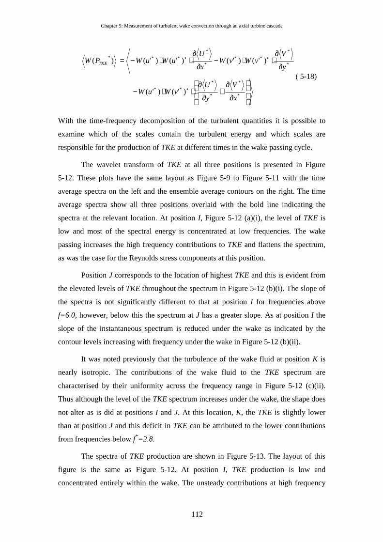
Chapter 5: Measurement of turbulent wake convection through an axial turbine cascade
112
∂
∂+
∂
∂⋅⋅−
∂
∂⋅⋅−
∂
∂⋅⋅−=
•
••
*
*
*
*
**
*
*
***
*
***
)'()'(
)'()'()'()'()(
x
V
y
UvWuW
y
VvWvW
x
UuWuWPW TKE
( 5-18)
With the time-frequency decomposition of the turbulent quantities it is possible to
examine which of the scales contain the turbulent energy and which scales are
responsible for the production of TKE at different times in the wake passing cycle.
The wavelet transform of TKE at all three positions is presented in Figure
5-12. These plots have the same layout as Figure 5-9 to Figure 5-11 with the time
average spectra on the left and the ensemble average contours on the right. The time
average spectra show all three positions overlaid with the bold line indicating the
spectra at the relevant location. At position I, Figure 5-12 (a)(i), the level of TKE is
low and most of the spectral energy is concentrated at low frequencies. The wake
passing increases the high frequency contributions to TKE and flattens the spectrum,
as was the case for the Reynolds stress components at this position.
Position J corresponds to the location of highest TKE and this is evident from
the elevated levels of TKE throughout the spectrum in Figure 5-12 (b)(i). The slope of
the spectra is not significantly different to that at position I for frequencies above
f=6.0, however, below this the spectrum at J has a greater slope. As at position I the
slope of the instantaneous spectrum is reduced under the wake as indicated by the
contour levels increasing with frequency under the wake in Figure 5-12 (b)(ii).
It was noted previously that the turbulence of the wake fluid at position K is
nearly isotropic. The contributions of the wake fluid to the TKE spectrum are
characterised by their uniformity across the frequency range in Figure 5-12 (c)(ii).
Thus although the level of the TKE spectrum increases under the wake, the shape does
not alter as is did at positions I and J. At this location, K, the TKE is slightly lower
than at position J and this deficit in TKE can be attributed to the lower contributions
from frequencies below f*=2.8.
The spectra of TKE production are shown in Figure 5-13. The layout of this
figure is the same as Figure 5-12. At position I, TKE production is low and
concentrated entirely within the wake. The unsteady contributions at high frequency
Chapter 5: Measurement of turbulent wake convection through an axial turbine cascade
113
occur at the time corresponding to the peak Reynolds shear stress. The high levels at
high frequencies again indicate a flattening of the spectrum under the wake due to
increased contributions from higher frequencies.
Position J is the location of peak TKE production. The spectrum of Figure
5-13(b)(i) shows an elevated level over the complete frequency range. Again, the
unsteady contributions cause the spectrum to flatten. Production at higher frequencies
is related to the passage of the counter rotating vortex pair, with an initial region of
elevated production followed a second higher peak after the passing of the vortex pair.
The wavelet transform of the production of TKE at the final point, K, is shown
in Figure 5-13 (c). This point exhibits the lowest level of TKE production as indicated
by the low levels of the time average spectrum of Figure 5-13 (c)(i). The ensemble
average spectrum shows smaller variations in the levels of TKE production through
the wake passing cycle. Furthermore, as in the case of TKE at this location, there is no
significant variation in the contributions from different scales.
In summary, the wavelet transforms show that a wide range of frequencies
contribute to the turbulence and that no isolated frequency is responsible for elevated
levels of TKE or TKE production. The spectral distributions of the wake and non-
wake fluid were observed to be different. The spectra within the anisotropic wake, at
positions I and J, have a greater contribution from the higher frequency components.
This has the effect of changing the shape of the TKE and TKE production spectra at
different times during the wake passing cycle. However, the TKE and TKE production
spectra of the more isotropic turbulence at position K showed less variation in shape
during the wake passing cycle.
5.6 Conclusions Measurements of the wake convected through a turbine blade row were made
using 2D LDA. The unprecedented resolution of the measurement grid and the
availability of the Reynolds stress components of the 2D flow provide a detailed
description of the ensemble averaged mean and turbulent flow fields.
The measurements confirm that the wake convection may be described by
simple kinematics with the wake fluid being bowed, re-orientated, elongated and
stretched as it passes through the blade passage. The counter rotating vortices pair

Chapter 5: Measurement of turbulent wake convection through an axial turbine cascade
114
established by the wake in the blade passage was clearly visible in plots of
perturbation vectors.
Measurements of the convected wake turbulence showed increased levels of
TKE due to the production of TKE by the interaction of the Reynolds stresses and the
strain rate field of the flow through a turbine blade. The wake fluid was shown to be
anisotropic until the point of peak TKE production was reached. The turbulence
production within the blade row was observed to produce a more nearly isotropic
turbulence and to increase the levels of TKE.
A novel algorithm for the wavelet analysis of unevenly sampled data was used
to perform the ensemble average wavelet analysis at three positions in the bladerow.
The Reynolds stress components were shown to be composed of a complete spectrum
of eddies with no particular eddy size responsible for any of the Reynolds stress
components, or the TKE or production of TKE. The wake fluid was characterised by a
flatter spectrum than the non-wake fluid.
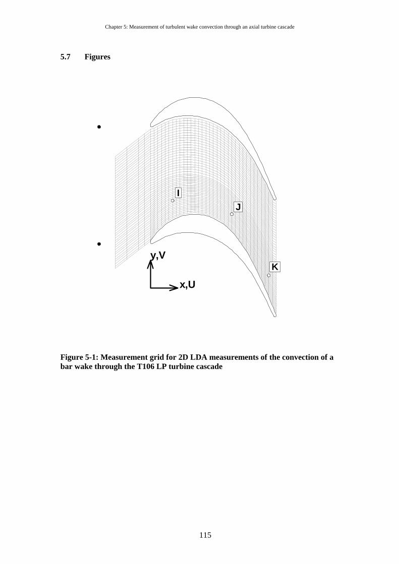
Chapter 5: Measurement of turbulent wake convection through an axial turbine cascade
115
5.7 Figures
x,U
y,V
IJ
K
Figure 5-1: Measurement grid for 2D LDA measurements of the convection of a bar wake through the T106 LP turbine cascade
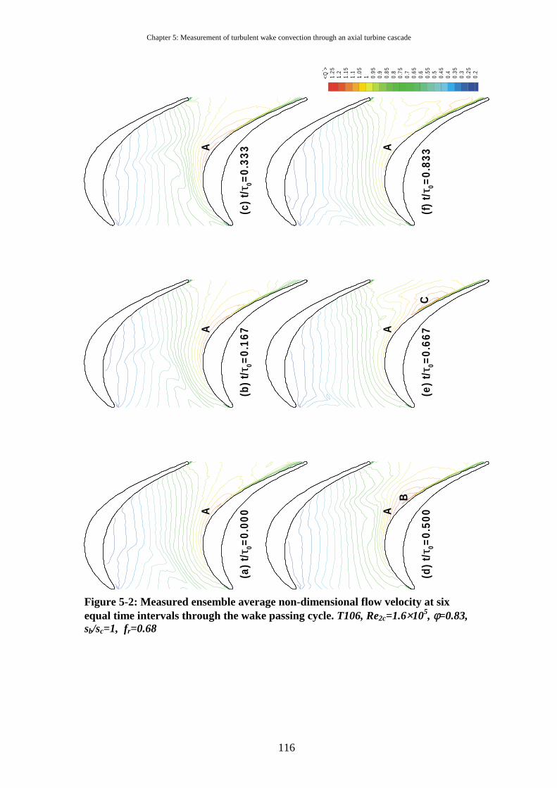
Chapter 5: Measurement of turbulent wake convection through an axial turbine cascade
116
(b)
t/τ 0=
0.1
67
A
(c)
t/τ 0=
0.33
3A
<Q* >
1.25
1.2
1.15
1.1
1.05
1 0.95
0.9
0.85
0.8
0.75
0.7
0.65
0.6
0.55
0.5
0.45
0.4
0.35
0.3
0.25
0.2
(f)
t/τ 0
=0.
833A
(a)
t/τ 0=
0.00
0A
(d)
t/τ 0=
0.5
00
BA
(e)
t/τ0=
0.6
67C
A
Figure 5-2: Measured ensemble average non-dimensional flow velocity at six equal time intervals through the wake passing cycle. T106, Re2c=1.6×10⁵, φ=0.83, sb/sc=1, fr=0.68
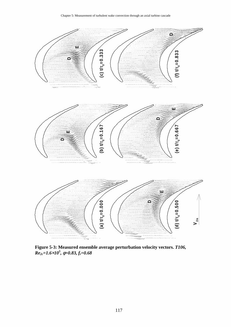
Chapter 5: Measurement of turbulent wake convection through an axial turbine cascade
117
(a)
t/τ 0=
0.0
00(b
)t/
τ 0=0
.16
7
DE
(c)
t/τ 0
=0.
333
D
E
(e)
t/τ 0=
0.6
67
D
E(f
)t/
τ 0=
0.83
3D
(d)
t/τ 0=
0.5
00
V2i
s
D
E
Figure 5-3: Measured ensemble average perturbation velocity vectors. T106, Re2c=1.6×10⁵, φ=0.83, fr=0.68
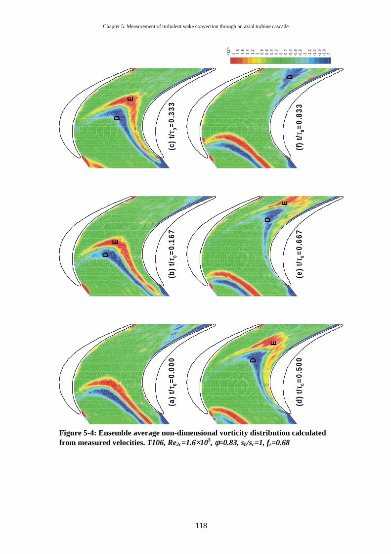
Chapter 5: Measurement of turbulent wake convection through an axial turbine cascade
118
(a)
t/τ0=
0.0
00(b
)t/
τ 0=
0.16
7
DE
(c)
t/τ 0
=0
.333
D
E
(d)
t/τ 0
=0.
500D
E
(e)
t/τ 0
=0
.66
7
D
E
< Ω* >
2 1.8
1.6
1.4
1.2
1 0.8
0.6
0.4
0.2
0 -0.2
-0.4
-0.6
-0.8
-1 -1.2
-1.4
-1.6
-1.8
-2
(f)
t/τ 0
=0
.833
D
Figure 5-4: Ensemble average non-dimensional vorticity distribution calculated from measured velocities. T106, Re2c=1.6×10⁵, φ=0.83, sb/sc=1, fr=0.68
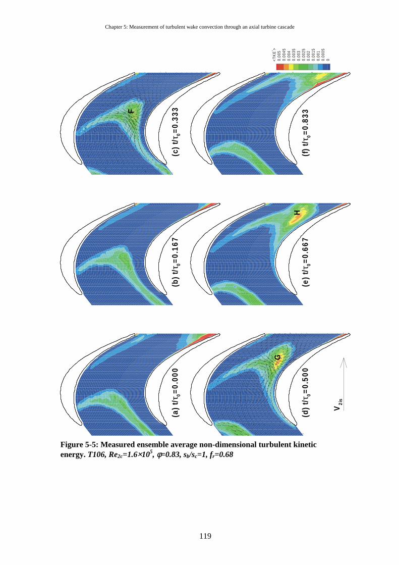
Chapter 5: Measurement of turbulent wake convection through an axial turbine cascade
119
(a)
t/τ 0
=0
.000
(b)
t/τ 0
=0.
167
<TK
E* >
0.00
50.
0045
0.00
40.
0035
0.00
30.
0025
0.00
20.
0015
0.00
10.
0005
0
(f)
t/τ 0
=0
.833
(e)
t/τ 0
=0
.66
7H
(c)
t/τ 0
=0
.333F
(d)
t/τ 0
=0.
50
0
G
V2
is
Figure 5-5: Measured ensemble average non-dimensional turbulent kinetic energy. T106, Re2c=1.6×10⁵, φ=0.83, sb/sc=1, fr=0.68
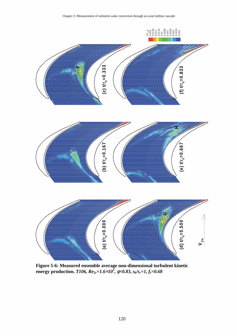
Chapter 5: Measurement of turbulent wake convection through an axial turbine cascade
120
<P
TK
E* >0.
016
0.01
450.
013
0.01
150.
010.
0085
0.00
70.
0055
0.00
40.
0025
0.00
1(f
)t/
τ 0=
0.8
33
(b)
t/τ 0
=0
.16
7(a
)t/τ
0=
0.0
00
(e)
t/τ0=
0.6
67
H
(c)
t/τ 0
=0
.33
3F
(d)
t/τ 0=
0.5
00
G
V2
is
Figure 5-6: Measured ensemble average non-dimensional turbulent kinetic energy production. T106, Re2c=1.6×10⁵, φ=0.83, sb/sc=1, fr=0.68
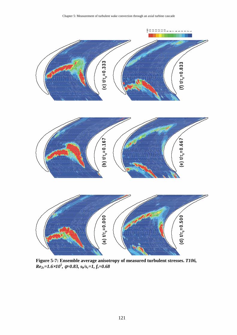
Chapter 5: Measurement of turbulent wake convection through an axial turbine cascade
121
(a)
t/τ0=
0.0
00
<α> 15 14 13 12 11 10 9 8 7 6 5 4 3 2 1
(f)
t/τ 0
=0
.833
(b)
t/τ 0
=0.
167
(c)
t/τ 0
=0
.333
(d)
t/τ 0
=0.
500
(e)
t/τ 0
=0
.66
7
Figure 5-7: Ensemble average anisotropy of measured turbulent stresses. T106, Re2c=1.6×10⁵, φ=0.83, sb/sc=1, fr=0.68
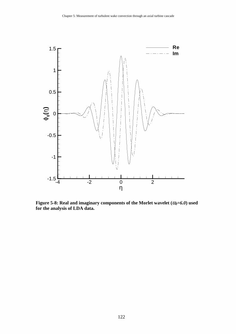
Chapter 5: Measurement of turbulent wake convection through an axial turbine cascade
122
η
ϕ 0(η
)
-4 -2 0 2-1.5
-1
-0.5
0
0.5
1
1.5 ReIm
Figure 5-8: Real and imaginary components of the Morlet wavelet (ω0=6.0) used for the analysis of LDA data.
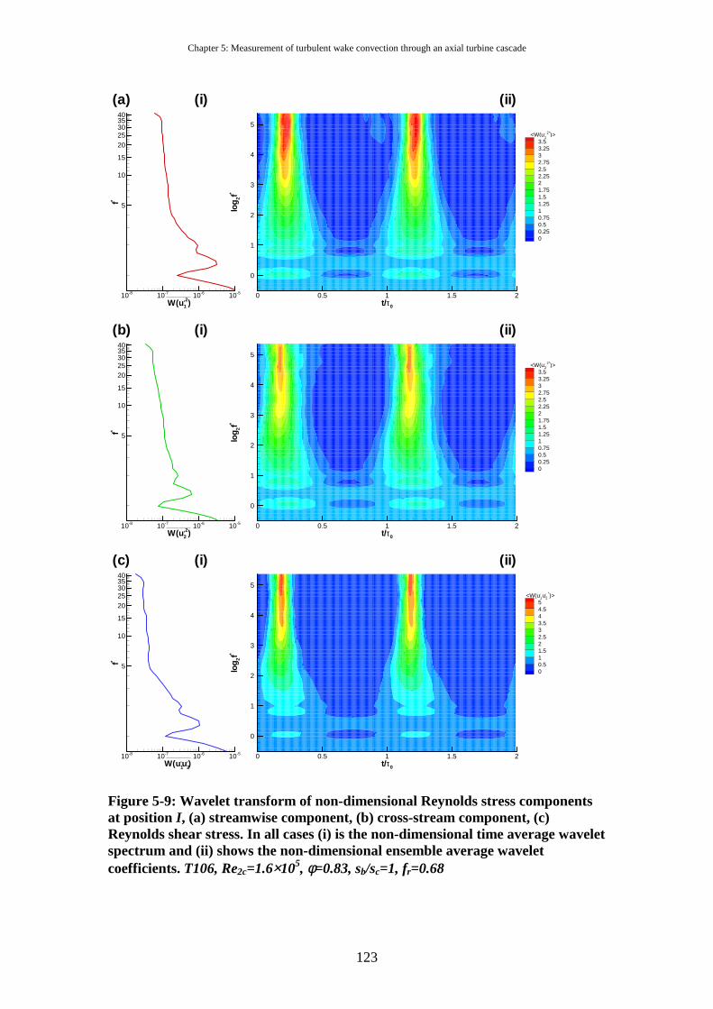
Chapter 5: Measurement of turbulent wake convection through an axial turbine cascade
123
W(u1,u2
,)
f*
10-8 10-7 10-6 10-5
5
10
15
2025303540
(c) (i)
t/τ0
log
2f*
0 0.5 1 1.5 2
0
1
2
3
4
5<W(u2
, 2*)>3.53.2532.752.52.2521.751.51.2510.750.50.250
(ii)
t/τ0
log
2f*
0 0.5 1 1.5 2
0
1
2
3
4
5<W(u1
, u2, *)>
54.543.532.521.510.50
(ii)
W(u1,2)
f*
10-8 10-7 10-6 10-5
5
10
15
2025303540
(a) (i)
W(u2,2)
f*
10-8 10-7 10-6 10-5
5
10
15
2025303540
(b) (i)
t/τ0
log
2f*
0 0.5 1 1.5 2
0
1
2
3
4
5<W(u1
, 2*)>3.53.2532.752.52.2521.751.51.2510.750.50.250
(ii)
Figure 5-9: Wavelet transform of non-dimensional Reynolds stress components at position I , (a) streamwise component, (b) cross-stream component, (c) Reynolds shear stress. In all cases (i) is the non-dimensional time average wavelet spectrum and (ii) shows the non-dimensional ensemble average wavelet coefficients. T106, Re2c=1.6×10⁵, φ=0.83, sb/sc=1, fr=0.68
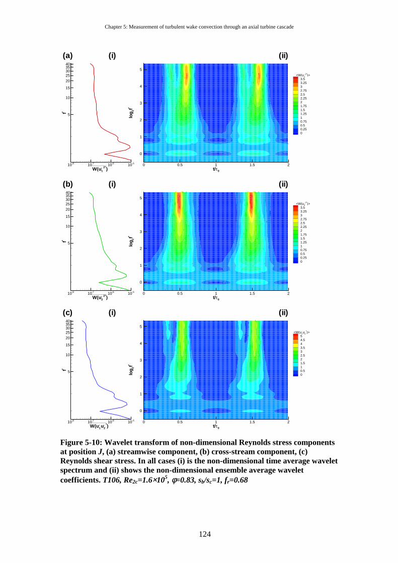
Chapter 5: Measurement of turbulent wake convection through an axial turbine cascade
124
t/τ0
log
2f*
0 0.5 1 1.5 2
0
1
2
3
4
5<W(u2
, 2*)>3.53.2532.752.52.2521.751.51.2510.750.50.250
(ii)
t/τ0
log
2f*
0 0.5 1 1.5 2
0
1
2
3
4
5<W(u1
, u2, *)>
54.543.532.521.510.50
(ii)
t/τ0
log
2f*
0 0.5 1 1.5 2
0
1
2
3
4
5<W(u1
, 2*)>3.53.2532.752.52.2521.751.51.2510.750.50.250
(ii)
W(u1, u2
, *)
f*
10-8 10-7 10-6 10-5
5
10
15
2025303540
(c) (i)
W(u1, 2*)
f*
10-8 10-7 10-6 10-5
5
10
15
2025303540
(a) (i)
W(u2, 2*)
f*
10-8 10-7 10-6 10-5
5
10
15
2025303540
(b) (i)
Figure 5-10: Wavelet transform of non-dimensional Reynolds stress components at position J, (a) streamwise component, (b) cross-stream component, (c) Reynolds shear stress. In all cases (i) is the non-dimensional time average wavelet spectrum and (ii) shows the non-dimensional ensemble average wavelet coefficients. T106, Re2c=1.6×10⁵, φ=0.83, sb/sc=1, fr=0.68
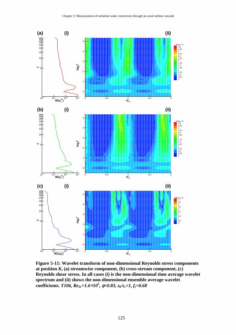
Chapter 5: Measurement of turbulent wake convection through an axial turbine cascade
125
W(u1,u2
,*)
f*
10-8 10-7 10-6 10-5
5
10
15
2025303540
(c) (i)
W(u1,2*)
f*
10-8 10-7 10-6 10-5
5
10
15
2025303540
(a) (i)
W(u2,2*)
f*
10-8 10-7 10-6 10-5
5
10
15
2025303540
(b) (i)
t/τ0
log
2f*
0 0.5 1 1.5 2
0
1
2
3
4
5<W(u1
, 2*)>3.53.2532.752.52.2521.751.51.2510.750.50.250
(ii)
t/τ0
log
2f*
0 0.5 1 1.5 2
0
1
2
3
4
5<W(u2
, 2*)>3.53.2532.752.52.2521.751.51.2510.750.50.250
(ii)
t/τ0
log
2f*
0 0.5 1 1.5 2
0
1
2
3
4
5<W(u1
, u2, *)>
54.543.532.521.510.50
(ii)
Figure 5-11: Wavelet transform of non-dimensional Reynolds stress components at position K, (a) streamwise component, (b) cross-stream component, (c) Reynolds shear stress. In all cases (i) is the non-dimensional time average wavelet spectrum and (ii) shows the non-dimensional ensemble average wavelet coefficients. T106, Re2c=1.6×10⁵, φ=0.83, sb/sc=1, fr=0.68
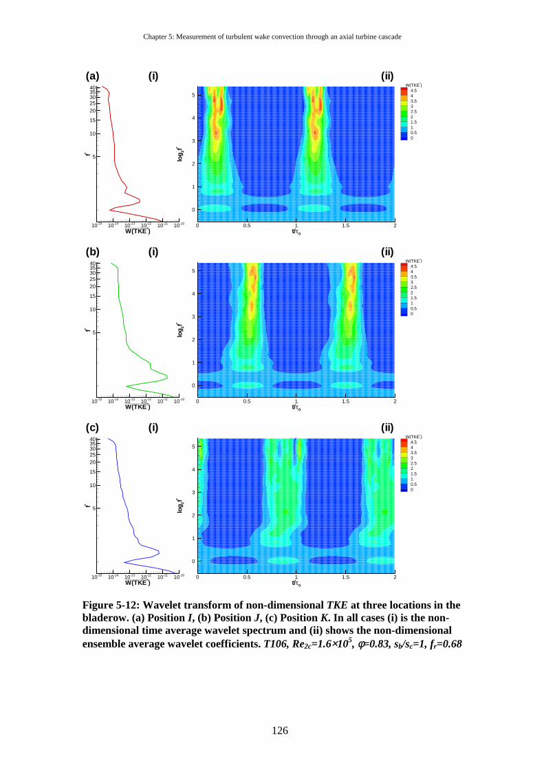
Chapter 5: Measurement of turbulent wake convection through an axial turbine cascade
126
t/τ0
log
2f*
0 0.5 1 1.5 2
0
1
2
3
4
5
W(TKE*)4.543.532.521.510.50
(ii)
t/τ0
log
2f*
0 0.5 1 1.5 2
0
1
2
3
4
5
W(TKE*)4.543.532.521.510.50
(ii)
W(TKE*)
f*
10-15 10-14 10-13 10-12 10-11 10-10
5
10
15
2025303540
(a) (i)
W(TKE*)
f*
10-15 10-14 10-13 10-12 10-11 10-10
5
10
15
2025303540
(c) (i)
W(TKE*)
f*
10-15 10-14 10-13 10-12 10-11 10-10
5
10
15
2025303540
(b) (i)
t/τ0
log
2f*
0 0.5 1 1.5 2
0
1
2
3
4
5
W(TKE*)4.543.532.521.510.50
(ii)
Figure 5-12: Wavelet transform of non-dimensional TKE at three locations in the bladerow. (a) Position I , (b) Position J, (c) Position K. In all cases (i) is the non-dimensional time average wavelet spectrum and (ii) shows the non-dimensional ensemble average wavelet coefficients. T106, Re2c=1.6×10⁵, φ=0.83, sb/sc=1, fr=0.68

Chapter 5: Measurement of turbulent wake convection through an axial turbine cascade
127
t/τ0
log
2f*
0 0.5 1 1.5 2
0
1
2
3
4
5
<W(PTKE*)>
54.543.532.521.510.50
(ii)
t/τ0
log
2f*
0 0.5 1 1.5 2
0
1
2
3
4
5
<W(PTKE*)>
54.543.532.521.510.50
(ii)
t/τ0
log
2f*
0 0.5 1 1.5 2
0
1
2
3
4
5
<W(PTKE*)>
54.543.532.521.510.50
(ii)
W(PTKE*)
f*
10-8 10-7 10-6 10-5 10-4
5
10
15
2025303540
(a) (i)
W(PTKE*)
f*
10-8 10-7 10-6 10-5 10-4
5
10
15
2025303540
(b) (i)
W(PTKE*)
f*
10-8 10-7 10-6 10-5 10-4
5
10
15
2025303540
(c) (i)
Figure 5-13: Wavelet transform of non-dimensional TKE production at three locations in the bladerow. (a) Position I , (b) Position J, (c) Position K. In all cases (i) is the non-dimensional time average wavelet spectrum and (ii) shows the non-dimensional ensemble average wavelet coefficients. T106, Re2c=1.6×10⁵, φ=0.83, sb/sc=1, fr=0.68
128
Chapter 6: Unsteady pressures measured on the suction surface of the T106 LP Turbine cascade
6.1 Introduction This Chapter presents unsteady surface pressures measured on the suction side
of the T106 LP turbine cascade. The surface pressures measured under the laminar
boundary layer upstream of the steady flow separation point were found to respond to
the wake passing in a quasi-steady manner as would be expected from the wake
convection measurements presented in Chapter 5. By contrast, in the region of the
steady flow separation bubble the arrival of the convecting wake produced high
frequency, short wavelength fluctuations in the ensemble averaged blade surface
pressure with a peak-to-peak magnitude of 30% of the exit dynamic head and a period
equal to approximately 20% of the bar passing period.
The existence of fluctuations in the ensemble averaged pressure traces
indicates that they are deterministic and are produced by coherent structures. Indeed,
the onset of the pressure fluctuations was found to lie beneath the convecting wake.
The coherent structures thus formed, propagate along a trajectory line drawn at half
the local freestream velocity.
The period of the oscillations depends on the Reynolds number, but not on the
bar passing frequency. An artificial disturbance generator was used to excite the
boundary layer and the pattern of ensemble average pressure traces thus measured
was found to be dissimilar to those measured with bar wakes. From these
observations, it is concluded that the coherent structures responsible for the pressure
fluctuations do not evolve purely from the periodic disturbance of random turbulent
fluctuations associated with the wake. Measurements performed with the boundary
layer tripped ahead of the separation point showed no oscillations in the ensemble
average pressure traces.
It is proposed that the coherent structures responsible for the large amplitude
pressure fluctuations are rollup vortices that form in the boundary layer as the wake
passes over inflexional velocity profiles and that the rollup of the separated shear
layer associated with the inflexional velocity profiles occurs by an inviscid Kelvin-
Helmholtz mechanism.

Chapter 6: Unsteady pressures measured on the suction surface of the T106 LP Turbine cascade
129
6.2 Time mean surface pressure distribution Ensemble averaged unsteady surface pressure measurements were made at
mid span on the suction surface of the T106 LP turbine cascade by the methods
described in Chapter 3. The Kulite pressure transducers, 1.6 mm in diameter (0.6%
surface length), were mounted flush with the blade surface and were located at 21
positions along the mid span of the suction surface of the blade. The locations of the
measurements are indicated by circles in Figure 6-1 (a).
The time averaged Cp distributions are shown in Figure 6-1(b). These surface
pressure measurements were made by traditional static pressure tappings located at
the same surface positions as the Kulites but a 25% span. The surface pressure
distribution measured at 25% span matches that measured at mid span in the absence
of the Kulites. For steady inflow, the pressure distribution is shown for both the
suction and pressure surface. Peak suction is located at s/s0=0.45. A separation bubble
is evident over the rear portion of the suction surface with separation at s/s0=0.60. The
pressure plateau, typically associated with the shear layer of a steady separation
bubble, extends to s/s0≈0.82. At this location, pressure recovery begins as the
separated shear layer undergoes transition and reattaches the boundary layer as
turbulent by s/s0=0.88.
For all cases with incoming wakes, only the suction surface Cp distribution is
shown. For the case of sb/sc=1 (fr=0.68) the time-mean surface pressure distribution
shows no sign of the separation bubble. In the time-mean, the separation bubble has
been suppressed by the wakes (Schulte, 1995). For the case of sb/sc=2 (fr=0.34),
where the blade surface boundary layer has longer to re-establish between wakes, the
time average surface pressure distribution indicates the presence of a separation
bubble. The separation and reattachment point for this case are indistinguishable from
the case for steady inflow; however, the pressure plateau is not as prevalent as in the
steady flow case. This is due to the time averaging of a flow, which is periodically
attached by the passing wake. The final surface pressure distribution on Figure 6-1 (b)
is for the case of sb/sc=2 with the boundary layer tripped by a 0.056 mm diameter wire
attached to the blade surface at s/s0≈0.44. The resulting turbulent boundary layer does
not separate. The Cp distribution is altered by the presence of the trip wire, with a
deceleration before and an over-acceleration after the trip-wire.
Chapter 6: Unsteady pressures measured on the suction surface of the T106 LP Turbine cascade
130
Near the leading edge of the suction surface, the Cp distributions differ for the
steady inflow case and the cases with bar passing. The differences are due to an
effective change in incidence of the incoming flow due to the bars of the wake
generator turning the inlet flow. This alteration of incidence is small and does not
significantly alter the pressure distribution downstream of peak suction.
6.3 Ensemble average suction surface pressures The ensemble averaged unsteady surface pressures measured on the suction
surface for the case of sb/sc=1 are presented as contours of Cp on an ST diagram in
Figure 6-3. The surface distance is non-dimensionalised by the suction surface length
and the time is non-dimensionalised by the bar passing period for the case sb/sc=1
(fr=0.68). The convection of the wake is evident and, upstream of the separation
point, is explained in terms of the negative jet model of Meyer (1958). The negative
jet, incident on the suction surface, causes the surface pressure to increase locally as
the wake convects over the suction surface. The increase in surface pressure
corresponds to the reduction in Cp observed in Figure 6-2.
As the wake arrives at the steady inflow separation location, a series of large
amplitude high frequency pressure oscillations arises. At s/s0=0.76 the peak-to-peak
amplitude of these pressure fluctuations is ∆Cp=0.3. The contours suggest that these
pressure waves travel with infinite celerity, however this is an anomaly of the
contouring algorithm and results from insufficient spatial resolution of the
measurements. These very large surface pressure fluctuations are the subject of
§6.3.1.
The distribution of Cp is shown at a series of five time instants through the
wake passing cycle in Figure 6-3. The time mean Cp distribution is shown for
comparison together with a series of vertical bars indicating the envelope of the
unsteady pressures at each sensor location. At t/τ0=0.0 the Cp distribution is very
similar to that of the time mean distribution. As the wake convects along the suction
surface, Cp is seen to reduce first over the forward part of the blade (t/τ0=0.2) under
the negative jet effect as described above. As the wake reaches mid chord (t/τ0=0.4),
the peak suction is reduced by ∆Cp=0.15. The pressure gradient at s/s0=0.6 is seen to
increase at this time. This has consequences for boundary layer separation. By
t/τ0=0.6 the wake has arrived at the separation location (s/s0=0.60) and the Cp
Chapter 6: Unsteady pressures measured on the suction surface of the T106 LP Turbine cascade
131
distribution over the rear of the blade is drastically altered. The Cp distributions at
t/τ0=0.62 and t/τ0=0.67 are included to demonstrate the magnitude of these pressure
oscillations. After the passage of the wake the Cp distribution returns to a state similar
to that of the time mean distribution as shown at t/τ0=0.8.
6.3.1 Unsteady surface pressures As remarked in §6.3 above, the nature of the pressure traces in the region
where the wake passes the steady flow separation bubble is markedly different from
upstream where the boundary layer is attached. Figure 6-4 shows a selection of raw
Kulite signals measured at s/s0=0.70 together with the ensemble-averaged calculated
from 256 ensembles. The ensemble averaging process can be seen to reduce the
random fluctuations between the wake passing events, however the large amplitude
pressure fluctuations are preserved in the ensemble average trace. The fact that these
pressure fluctuations are evident in the raw and the ensemble-averaged pressure traces
indicates that they are formed by deterministic coherent structures in the flow.
Ensemble averaged pressure traces measured over the rear half of the suction
surface, are shown in Figure 6-5. The data is the same as that presented in Figure 6-2.
The vertical axis indicates the surface location non-dimensionalised by the suction
surface length, and the horizontal axis is time, non-dimensionalised as before. The
dash-dot lines indicate the surface location of each Kulite while the solid lines are the
ensemble-averaged traces of the measured surface pressure fluctuation. The
magnitude of the pressure traces is arbitrary but consistent between the traces. At
s/s0=0.76 the peak-to-peak amplitude of the pressure fluctuations is 30% of exit
dynamic pressure and the period is approximately 20% of the bar passing period
(fr=0.68).
The line, labelled A, in Figure 6-5 is a trajectory line drawn at the freestream
velocity as calculated from the Cp distribution presented in Figure 6-1 (b). The onset
of the large amplitude pressure oscillations in Figure 6-5, fall along line A. From this
it is possible to conclude that the onset of the pressure oscillations is dictated by the
wake, which convects with the freestream velocity. The onset is not controlled by the
convection of turbulent spots nor instability waves within the boundary layer as these
convect slower than the freestream. Similarly, the onset is not controlled by an
Chapter 6: Unsteady pressures measured on the suction surface of the T106 LP Turbine cascade
132
acoustic mechanism as for a low Mach number flow this would travel ahead of the
convecting wake.
The pressure fluctuations are observed to originate between the traces at
s/s0=0.57 and s/s0=0.63. Thereafter, intense amplification occurs up to s/s0=0.70 and
after that the amplitude of the oscillations remains approximately constant. The period
of the oscillations is also constant downstream of s/s0=0.70. The amplitude of the
fluctuations reduces slightly downstream of s/s0=0.82. This region corresponds to the
pressure recovery region of the steady separation bubble and is typically associated
with transition in a separation bubble. With increased levels of turbulence and
turbulent mixing that result from transition, the ensemble-average pressure
fluctuations decrease in amplitude.
The pairs of trajectory lines labelled C, D and E are drawn at half the local
freestream velocity as calculated from the Cp distribution of Figure 6-1 (b). These
lines are positioned to trace the convection of the maxima and minima of the pressure
fluctuations. The trajectory lines do not pass through the pressure traces at these
points, but rather pass through the corresponding s/s0 lines at the same time as the
maxima or minima occur. From Figure 6-5, it is apparent that all the maxima and
minima have the same trajectory and that this trajectory is half the freestream
velocity. The coherent structures responsible for the pressure fluctuations thus travel
at half the freestream velocity except in the region indicated by trajectory lines B that
are drawn by hand to track the pressure maxima and minima between s/s0=0.63 and
s/s0=0.70. The slope of lines B is lower than that of lines C, D and E. This indicates
that the coherent structures convect slower than half the freestream velocity in this
region.
The number of maxima and minima in the ensemble averaged pressure traces
is not the same at every sensor location in Figure 6-5. At s/s0=0.7 there is only one
maxima and one minima observed, however, at s/s0=0.82 there are three sets of
maxima and minima. The appearance of more than one coherent structure is due to
the different trajectories of the onset and convection of these structures. Once formed
the structures convect slower than the wake thus allowing the wake to generate new
structures at points further downstream as it passes over the undisturbed inflexional
profiles of the separating boundary layer.
Chapter 6: Unsteady pressures measured on the suction surface of the T106 LP Turbine cascade
133
By extending the trajectory lines C to intersect line A, the origin of structure C
is seen to be at s/s0≈0.60. However, by s/s0≈0.86 structure C disappears. The
convection speed of coherent structure C is lower than the convection speed of the
leading edge of a turbulent spot. The disappearance of C is attributed to turbulent
spots formed at an upstream16 location overtaking the coherent structure. This
turbulence destroys the coherence of structure C.
6.3.2 The effect of bar passing frequency Figure 6-6 shows the ensemble averaged unsteady surface pressures for the
identical flow condition in Figure 6-5, but with double the bar spacing so that sb/sc=2
(fr=0.34). Both the time axis and the scale of the pressure traces are identical to that of
Figure 6-5.
The pressure fluctuations are again observed as the wake passes over the
region of the steady flow separation bubble. No change in the onset location is evident
and the period of oscillation is the same as before. The period of the pressure
fluctuations are thus independent of the bar passing frequency. The pattern of the
pressure oscillations is also the same as for the higher bar passing frequency up to
s/s0=0.86 but their magnitude is larger for the current case with lower bar passing
frequency.
The lower bar passing frequency gives the boundary layer more time to re-
establish between wake passing events. In this time a series of pressure oscillations,
smaller in magnitude and of lower frequency arise downstream of s/s0=0.88. The
pattern of these pressure traces is different to those resulting from the wake-separation
bubble interaction. They are more nearly sinusoidal with similar positive and negative
amplitudes. The fact that these oscillations may be ensemble averaged is remarkable
and indicates that they too are caused by coherent structures in the re-establishing
boundary layer. As in Chapter 4, oscillations of this type were attributed to natural
transition phenomena.
16 At this stage of the argument, no mechanism for the creation of turbulent spots has been suggested. This will be addressed in Chapter 7.
Chapter 6: Unsteady pressures measured on the suction surface of the T106 LP Turbine cascade
134
6.3.3 The effect of a boundary layer trip The effect of a trip wire fixed to the surface of the blade is to cause transition
of the boundary layer at the trip wire location. Downstream of the trip wire the
boundary layer is turbulent and attached throughout the wake passing cycle.
Figure 6-7 shows ensemble averaged pressure traces for identical flow
conditions to those presented in Figure 6-6, but with a trip wire at s/s0=0.44.
Immediately obvious is the absence of the pressure fluctuations downstream of
s/s0=0.60. The coherent structures responsible for the pressure fluctuations are thus
only formed when the wake interacts with the separating boundary layer.
6.3.4 The effect of Reynolds number on pressure fluctuations It was established in §6.3.2 that the period of the large amplitude pressure
fluctuations is independent of the bar passing frequency. However, the period of the
pressure fluctuations is dependent on Reynolds number. The pressure traces at a
Reynolds number of Re2C=1.6×10⁵ and at a Reynolds number Re2C=2.0×10⁵, which is
125% higher, are shown in Figure 6-9. Pressure traces are shown at s/s0=0.63 and
s/s0=0.70 for both Reynolds numbers. These surface positions are both within the
laminar shear layer of the steady flow separation bubble. The vertical axis is surface
location with the magnitude of the pressure traces arbitrarily scaled. The time axis in
this plot is dimensional. The pressure traces are shown only for the time associated
with large oscillations resulting from the wake-separation interaction. It is apparent
that the period of the pressure oscillations is not the same at the different Reynolds
numbers. The time offset between the two sets of pressure traces is due to difference
in the absolute time of the trigger used for the ensemble averaging of the different
Reynolds number flow conditions.
The period of the pressure oscillations for Re2C=2.0×10⁵ is marked by the blue
lines L1 at s/s0=0.63 and L2 at s/s0=0.72. Similarly, the period for Re2C=1.6×10⁵ is
marked by red lines. Two more blue lines are drawn with solid arrows. As labelled,
these are 125% of the length of L1 and L2. From this it is clear that the period of the
oscillations at s/s0=0.63 and s/s0=0.72 are inversely proportional to the Reynolds
number.
The convective time scale,
Chapter 6: Unsteady pressures measured on the suction surface of the T106 LP Turbine cascade
135
U
Cconv ∝τ ( 6-1)
and viscous diffusion time scale,
U
x
x
x
visc ∝
∝∝νν
δτ
2
2 Re* ( 6-2)
are indistinguishable for a given velocity distribution as the ratio of x to C is constant.
It is thus not possible to determine if the large pressure fluctuations are related to
viscous or convective phenomena.
A correlation for the period of the disturbance with the maximum
amplification rate in the Falkner-Skan velocity profiles over the whole range of
pressure gradient parameter is given by Walker (1989) as
2*
23
Re2.3
1
Uf critcrit −=∝
δ
ντ ( 6-3)
This correlation was shown to reliably predict the frequency of Tollmein-
Schlichting waves17 in Chapter 4. The period of a viscous instability in a highly
decelerated boundary layer is thus expected to vary non-linearly with Reynolds
number. The observed linear relationship between the period of the pressure
fluctuations and Reynolds number demonstrates that a viscous stability mechanism is
not responsible for the large amplitude pressure fluctuation. Villermaux (1998)
showed that inviscid instability processes have a negligible Reynolds number
dependence and so an inviscid instability mechanism is not excluded.
6.3.5 The interaction of a wave packet with the separating boundary layer In order to separate the effects of wake turbulence and the negative jet effect a
series of measurements were performed with the boundary layer periodically
perturbed by the artificial disturbance generator described in Chapter 3. The artificial
disturbance generator was driven with a square wave pulse to excite as broad a
frequency spectrum as possible. Such a disturbance simulates the effect of the
periodically applied disturbances associated with the wake turbulence but without the
negative jet effect of the convected wake. 17 Obremski et al (1969) state that matching of the vorticity distribution between 0.1<y/δ<0.9 is the most reliable way of reproducing nearly identical stability characteristics.
Chapter 6: Unsteady pressures measured on the suction surface of the T106 LP Turbine cascade
136
The disturbances were generated at s/s0=0.57, this is in the decelerating
boundary layer before the steady flow separation point. The frequency of the
perturbations was set to match the bar passing frequency for Re2C=1.6×10⁵ and
sb/sc=2. The ensemble averaged surface pressure distribution measured downstream
of this location is presented in Figure 6-8.
As for the case with bar passing, ensemble average pressure fluctuations are
observed with strong amplification between s/s0=0.63 and s/s0=0.70. However the
amplitude of these pressure fluctuations is smaller and the period is about half that of
the wake passing case. The pattern of pressure fluctuations is different to the wake
passing case as highlighted by the inset frame which shows the traces overlaid at
s/s0=0.70.
From these measurements, it is possible to conclude that the coherent
structures responsible for the large amplitude pressure fluctuations are not only a
result of the amplification of disturbances associated with wake turbulence by the
velocity profiles of the steady flow separation region.
6.4 The formation of coherent structures in a separating shear layer The evolution of artificial disturbances in boundary layers has been studied by
researchers interested in boundary layer stability. The classical stability experiments,
such as those of Schubauer and Skramstad (1947), were performed by using a
vibrating ribbon to excite instability waves in a boundary layer. By varying the
frequency of excitation and altering the flow speed to change the boundary layer
thickness, the neutral stability curve was determined. Good agreement was found
between the experimentally determined neutral stability curve and that predicted by
linear stability theory.
The evolution of a wave packet in a zero pressure gradient boundary layer was
studied experimentally and theoretically by Gaster (1981). An acoustic driver was
used to introduce a disturbance into the boundary layer and the evolution of the
resulting wave packet was measured by a probe at a fixed location downstream of the
disturbance. Measurements in the boundary layer downstream of the disturbance
location were made across the span of the plate and showed a wave packet to be
formed. Gaster was able to calculate the convected wave packet. Linear stability
theory was used to predict the behaviour of all the discrete modes excited in the
Chapter 6: Unsteady pressures measured on the suction surface of the T106 LP Turbine cascade
137
boundary layer and this information was then used to compute the resulting wave
packet by a summation over all the modes with only the dominant mode capable of
amplification and a locally parallel flow approximation. The measurements and
calculations of Gaster (1981) are reproduced in Figure 6-10. The agreement between
the calculated and measured wave packets is good. The discrepancies between the two
are attributed to non-linear effects.
In the experiment of Gaster (1981), the boundary layer was excited by an
acoustic driver through a small hole in the flat plate. A square pulse was used to
excite a broad spectrum of disturbances. The linear instability mechanism associated
with the flat plate boundary layer profile lead to amplification of particular
frequencies. The exponential amplification rate associated with linear instability
rapidly lead to the dominance of the most amplified mode. Such a selective
amplification process acts as a filter that leads to a single mode becoming dominant.
This selective amplification mechanism resulted in a coherent structure being formed
in the boundary layer, in this case a travelling wave packet.
The instability mechanism governing the evolution of a wave packet in a
separation bubble was investigated experimentally by Watmuff (1999). A pressure
gradient was imposed on a large flat plate so that a laminar separation bubble was
formed. An artificial disturbance was periodically generated at the minimum pressure
point (peak suction) and hot-wire measurements were made to track the evolution of
the resulting wave packet. The disturbance was observed to decay in the boundary
layer upstream of separation. After the separation location, the rate of decay reduced
but the disturbances continued to decay. The character of the disturbance was also
observed to change upon entering the separated region. At a later point after
separation, the amplitude of the disturbances began to increase and the wave packet
disturbance was observed to grow with the same exponential growth rate as
background disturbances. This indicates linear behaviour, as the growth rate is
independent of the initial amplitude of the disturbance. Dovgal and Kozlov (1990)
also found the growth rate of two-dimensional waves in a separation bubble to be
independent of their initial magnitude even when the amplitude of the disturbance
reached 20% of the freestream velocity. The end of the exponential growth region
corresponds to the end of the linear region and this was found to coincide with a rapid
increase in the boundary layer thickness.
Chapter 6: Unsteady pressures measured on the suction surface of the T106 LP Turbine cascade
138
The location of the maximum amplitude of the wave packet was observed to
follow the trajectory of the inflexion points in the boundary layer velocity profile and
contours of the spanwise vorticity revealed a cat’s eye pattern, which is characteristic
of a Kelvin-Helmholtz breakdown in the shear layer. This evidence allowed Watmuff
to conclude that the instability mechanism governing the amplification of the wave
packet in a separation bubble is predominantly inviscid.
Further measurements by Watmuff (1999) were performed with a flying X-
wire probe and an exceptionally fine three-dimensional measurement grid. Figure
6-11 and Figure 6-12 are reproduced from Watmuff (1999). A series of contour plots
of spanwise vorticity at the centre line of the wave packets (Figure 6-11) shows the
cat’s eye patterns reminiscent of the initial stages of rollups in a shear layer. The
evolution of the cat’s eye pattern into four regions of concentrated spanwise vorticity
is apparent in Figure 6-11. However, the three-dimensional data, shown as a series of
iso-vorticity surfaces in Figure 6-12, reveals the rollup is actually three-dimensional.
The large amplitude three-dimensional waves resulting from the inviscid
amplification mechanism in the separation bubble’s shear layer can be seen to evolve
into a group of large-scale vortex loops. The three-dimensional rollups develop legs,
which move together. The coming together of the legs enforces the curvature of the
central region. This in turn accelerates the central region away from the wall forming
elongated vortex loops. These vortex loops remain as discernable coherent structures
up to twenty boundary layer thicknesses downstream in the fully turbulent boundary
layer.
The work of Gaster (1981) and Watmuff (1999) shows that the selective
amplification associated with boundary layer stability, both viscid and inviscid,
provides a mechanism able to form coherent structures. It is proposed that the
deterministic coherent structures responsible for the measured pressure fluctuations
are formed by the selective amplification of such an instability mechanism.
6.5 Visualisation of the instantaneous flow field using PIV PIV is essentially a quantitative flow visualisation technique. Two images of a
seeded flow are used to determine the fluid velocity by tracking the displacement of
the suspended particles over a known time as described in Chapter 3. The PIV
technique provides quantitative data of the instantaneous flow field, however, for the

Chapter 6: Unsteady pressures measured on the suction surface of the T106 LP Turbine cascade
139
current purpose of identifying coherent structures, an instantaneous flow visualisation
is sufficient.
The results of a PIV measurement for a small area on the suction surface of
the T106 LP turbine cascade for the phase t/τ0=0.85 are shown in Figure 6-13. The
position of the measurement relative to the blade is shown in Figure 6-13 (a) and
corresponds to the region between s/s0=0.8 and s/s0=0.9. In order to achieve sufficient
resolution in the boundary layer a large zoom factor was used permitting only a small
section of the blade surface to be viewed.
The instantaneous vector map, calculated as described in Chapter 318, is shown
in Figure 6-13 (c). Two vortices are visible in the boundary layer at labels A and B.
Instantaneous streamlines calculated from the vector map are shown in Figure 6-13
(d) and confirm that the structures at A and B are vortices embedded in the boundary
layer. A number of PIV measurements were made and not all showed identical
features to the results of Figure 6-13. The vortices were not always present and their
size and position varied at the same phase relative to the bar passing.
The vorticity of the vortices at A and B is of the same sense as the boundary
layer vorticity. The vortex centres are separated by approximately 5% of the suction
surface length with their centres at approximately a third of the local time average
boundary layer thickness. It is argued below that these vortices are responsible for the
measured pressure fluctuations.
6.6 The source of surface pressure fluctuations Saathoff and Melbourne (1997) conducted an investigation into the cause of
large pressure fluctuations occurring near the leading edges of sharp-edged bluff
bodies19. A long two-dimensional rectangular prism was mounted in a wind tunnel
and the surface pressure was measured under the separation bubble that formed at the
leading edge. Flow visualisation was performed with a laser light sheet with the flow
seeded from the model’s leading edge with a fine powder consisting of a mixture of
balsa and china clay. A high-speed cine camera was used to simultaneously capture
flow visualisation pictures and an oscilloscope output from the pressure transducers.
18 The author is indebted to Mr D Hollis for his assistance in acquiring the PIV data. The processing of the PIV images is the work of Mr Hollis. 19 A major cause of damage in windstorms is large pressure fluctuations occurring near the leading edges of buildings. The sharp-edged bluff body is intended to simulate the leading edge of a building in wind.
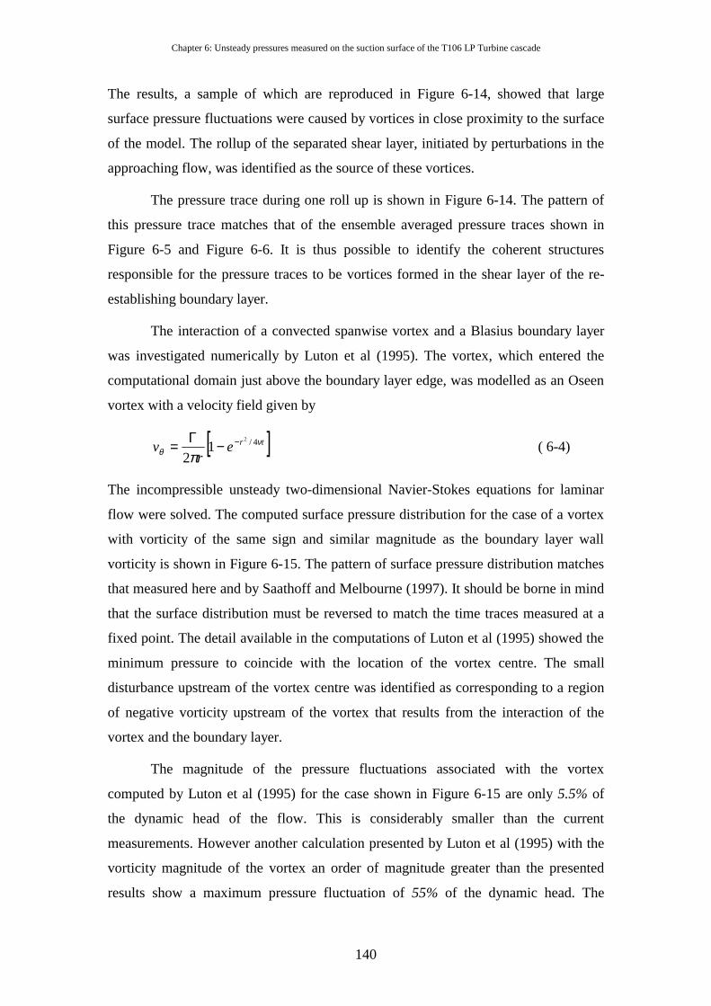
Chapter 6: Unsteady pressures measured on the suction surface of the T106 LP Turbine cascade
140
The results, a sample of which are reproduced in Figure 6-14, showed that large
surface pressure fluctuations were caused by vortices in close proximity to the surface
of the model. The rollup of the separated shear layer, initiated by perturbations in the
approaching flow, was identified as the source of these vortices.
The pressure trace during one roll up is shown in Figure 6-14. The pattern of
this pressure trace matches that of the ensemble averaged pressure traces shown in
Figure 6-5 and Figure 6-6. It is thus possible to identify the coherent structures
responsible for the pressure traces to be vortices formed in the shear layer of the re-
establishing boundary layer.
The interaction of a convected spanwise vortex and a Blasius boundary layer
was investigated numerically by Luton et al (1995). The vortex, which entered the
computational domain just above the boundary layer edge, was modelled as an Oseen
vortex with a velocity field given by
[ ]trer
v νθ π
4/2
12
−−Γ= ( 6-4)
The incompressible unsteady two-dimensional Navier-Stokes equations for laminar
flow were solved. The computed surface pressure distribution for the case of a vortex
with vorticity of the same sign and similar magnitude as the boundary layer wall
vorticity is shown in Figure 6-15. The pattern of surface pressure distribution matches
that measured here and by Saathoff and Melbourne (1997). It should be borne in mind
that the surface distribution must be reversed to match the time traces measured at a
fixed point. The detail available in the computations of Luton et al (1995) showed the
minimum pressure to coincide with the location of the vortex centre. The small
disturbance upstream of the vortex centre was identified as corresponding to a region
of negative vorticity upstream of the vortex that results from the interaction of the
vortex and the boundary layer.
The magnitude of the pressure fluctuations associated with the vortex
computed by Luton et al (1995) for the case shown in Figure 6-15 are only 5.5% of
the dynamic head of the flow. This is considerably smaller than the current
measurements. However another calculation presented by Luton et al (1995) with the
vorticity magnitude of the vortex an order of magnitude greater than the presented
results show a maximum pressure fluctuation of 55% of the dynamic head. The

Chapter 6: Unsteady pressures measured on the suction surface of the T106 LP Turbine cascade
141
pressure fluctuation depends on the location of the distance of the vortex from the
wall as well as the strength of vortex.
6.7 Description of Mechanism
6.7.1 Hot wire measurements In order to establish the state of the boundary layer during the wake passing
cycle, a series of hot wire traverses were performed at the same surface locations as
the surface pressures were measured.
Figure 6-16 shows the traverse measured at s/s0=0.70 for the case of the
artificial disturbance. The contour plots of perturbation velocity show the wave
packet. These results are very similar to those of Watmuff (1999). The adjacent
ensemble average velocity profiles, shown at selected time instants, demonstrate the
inflexional nature of the profiles in the shear layer of a separation bubble. The profile
shape does not change much as the wave packet passes. The wave packet travels at
the height of the inflexion point in the profiles. This agrees with the observations of
Watmuff and indicates an inviscid instability mechanism.
The hot wire traverse results for the case of wake passing are shown in Figure
6-16 (b). The negative jet effect associated with the wake is apparent as an
acceleration before and deceleration after the passing of the wake in the perturbation
velocity contours and the ensemble average velocity profiles. Of primary interest are
the velocity profiles before the wake arrival (purple and red line in Figure 6-16 (b)).
These profiles are similar to those in Figure 6-16 (a) and have an inflexion point. The
turbulent to laminar relaxation of the boundary layer under a strong adverse pressure
gradient results in inflexional boundary layer profiles. The inviscid instability
mechanism, found to be responsible for the amplification of the artificial wave
packets, is thus applicable to the wake passing case. Moreover, the contours of
perturbation velocity show the peak velocity perturbations at the height of the
boundary layer inflexion. This again indicates an inviscid mechanism is dominant.
6.7.2 A schematic view of the origin of pressure fluctuations A schematic view of mechanism responsible for the high amplitude pressure
fluctuations is presented in Figure 6-17. The upper plot shows the measured mean
pressure distribution over the rear suction surface of the T106 LP turbine cascade for
steady flow. Also shown is an inviscid pressure distribution. The difference between
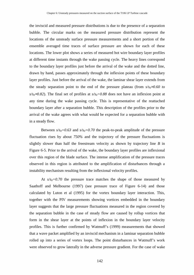
Chapter 6: Unsteady pressures measured on the suction surface of the T106 LP Turbine cascade
142
the inviscid and measured pressure distributions is due to the presence of a separation
bubble. The circular marks on the measured pressure distribution represent the
locations of the unsteady surface pressure measurements and a short portion of the
ensemble averaged time traces of surface pressure are shown for each of these
locations. The lower plot shows a series of measured hot wire boundary layer profiles
at different time instants through the wake passing cycle. The heavy lines correspond
to the boundary layer profiles just before the arrival of the wake and the dotted line,
drawn by hand, passes approximately through the inflexion points of these boundary
layer profiles. Just before the arrival of the wake, the laminar shear layer extends from
the steady separation point to the end of the pressure plateau (from s/s0≈0.60 to
s/s0≈0.82). The final set of profiles at s/s0=0.88 does not have an inflexion point at
any time during the wake passing cycle. This is representative of the reattached
boundary layer after a separation bubble. This description of the profiles prior to the
arrival of the wake agrees with what would be expected for a separation bubble with
in a steady flow.
Between s/s0=0.63 and s/s0=0.70 the peak-to-peak amplitude of the pressure
fluctuation rises by about 750% and the trajectory of the pressure fluctuations is
slightly slower than half the freestream velocity as shown by trajectory line B in
Figure 6-5. Prior to the arrival of the wake, the boundary layer profiles are inflexional
over this region of the blade surface. The intense amplification of the pressure traces
observed in this region is attributed to the amplification of disturbances through a
instability mechanism resulting from the inflexional velocity profiles.
At s/s0=0.70 the pressure trace matches the shape of those measured by
Saathoff and Melbourne (1997) (see pressure trace of Figure 6-14) and those
calculated by Luton et al (1995) for the vortex boundary layer interaction. This,
together with the PIV measurements showing vortices embedded in the boundary
layer suggests that the large pressure fluctuations measured in the region covered by
the separation bubble in the case of steady flow are caused by rollup vortices that
form in the shear layer at the points of inflexion in the boundary layer velocity
profiles. This is further confirmed by Watmuff’s (1999) measurements that showed
that a wave packet amplified by an inviscid mechanism in a laminar separation bubble
rolled up into a series of vortex loops. The point disturbances in Watmuff’s work
were observed to grow laterally in the adverse pressure gradient. For the case of wake
Chapter 6: Unsteady pressures measured on the suction surface of the T106 LP Turbine cascade
143
passing, where the disturbance sources may be viewed as a two-dimensional strip of
convecting wake fluid, the amplified disturbances would not break down into vortex
loops, but rather a more two-dimensional spanwise rollup vortex. Rollup vortices
formed in a shear layer convect at the mean velocity of the shear layer. For the shear
layer of a separation bubble the mean velocity would be approximately half the
freestream velocity as the wall velocity is zero. The coherent structures responsible
for the pressure fluctuations were identified to convect at half the freestream velocity
in §6.3.1above. This adds to the argument that the coherent structures responsible for
the large amplitude surface pressure fluctuations are rollup vortices formed in the
separated shear layer associated with the inflexional boundary layer velocity profiles.
The pressure traces for the artificial disturbance shown in Figure 6-8 do not
have the same pattern as those for the case with wakes. The hot wire traverses
highlighted the similarity between these measurements and those of Watmuff (1999)
and indicate that the source of the pressure oscillations in this case is a wave packet
rather than a rollup vortex. The pattern of the pressure fluctuations for the artificial
disturbance is similar to that in the region of natural transition. The coherent
structures in the natural transition region identified in §6.3.2 and Figure 6-6 can thus
be identified as waves rather than vortices. This supports their identification as
Tollmein-Schlichting waves arising during the turbulent-laminar transition as
identified in Chapter 4.
6.8 Conclusions Measurements of the unsteady surface pressure on the T106 LP turbine
cascade showed unexpected large amplitude fluctuations in surface pressure as the
wake convected over the location of the steady flow separation bubble. The pressure
oscillations were suppressed when the boundary layer was tripped indicating that the
unsteady decelerated laminar boundary layer was necessary for the development of
the pressure oscillations. The pressure oscillations were found to be generated as the
wake passed over the region covered by the separation bubble in the case of steady
flow and to convect at half the local freestream velocity. The pressure oscillations
were unaltered when the bar passing frequency was halved but were found to be
inversely proportional to the Reynolds number. Artificial disturbances to the
boundary layer were also found to trigger large amplitude pressure fluctuations,
however the ensemble averaged pressure traces that resulted had a different character.

Chapter 6: Unsteady pressures measured on the suction surface of the T106 LP Turbine cascade
144
PIV measurements, used as a quantitative flow visualisation technique,
identified vortices present in the boundary layer and it was shown by reference to
literature that these vortices are responsible for the pressure oscillations.
In the ensemble-averaged measurements, the vortices appear as coherent and
deterministic structures. Hot wire boundary layer traverses confirmed the existence of
inflexional velocity profiles prior to the arrival of the wake. It is proposed that an
inviscid instability mechanism associated with the inflexional boundary layer velocity
profiles is responsible for the formation of the vortices that are responsible for the
pressure fluctuations.
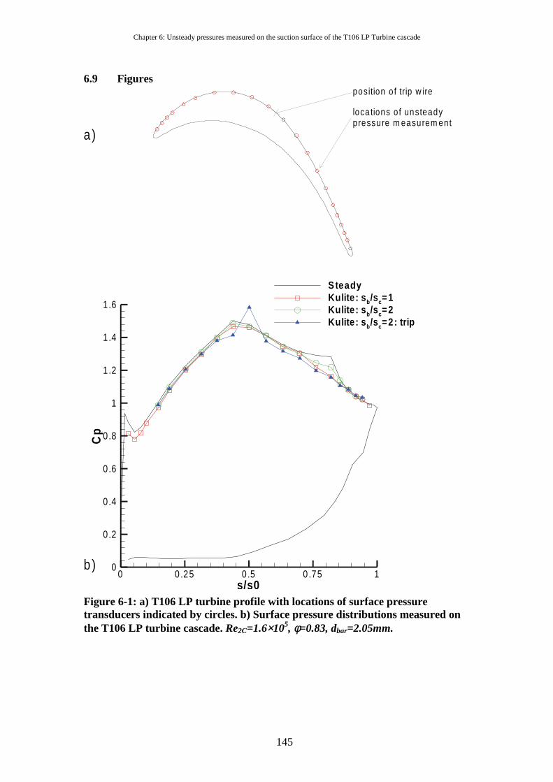
Chapter 6: Unsteady pressures measured on the suction surface of the T106 LP Turbine cascade
145
6.9 Figures
s/s0
Cp
0 0 .25 0.5 0 .75 10
0.2
0.4
0.6
0.8
1
1.2
1.4
1.6
S teadyKulite : s b/s c=1Kulite : s b/s c=2Kulite : s b/s c=2 : trip
a)
b)
loca tions o f unsteadypressu re m easurem ent
position o f trip w ire
Figure 6-1: a) T106 LP turbine profile with locations of surface pressure transducers indicated by circles. b) Surface pressure distributions measured on the T106 LP turbine cascade. Re2C=1.6×10⁵, φ=0.83, dbar=2.05mm.
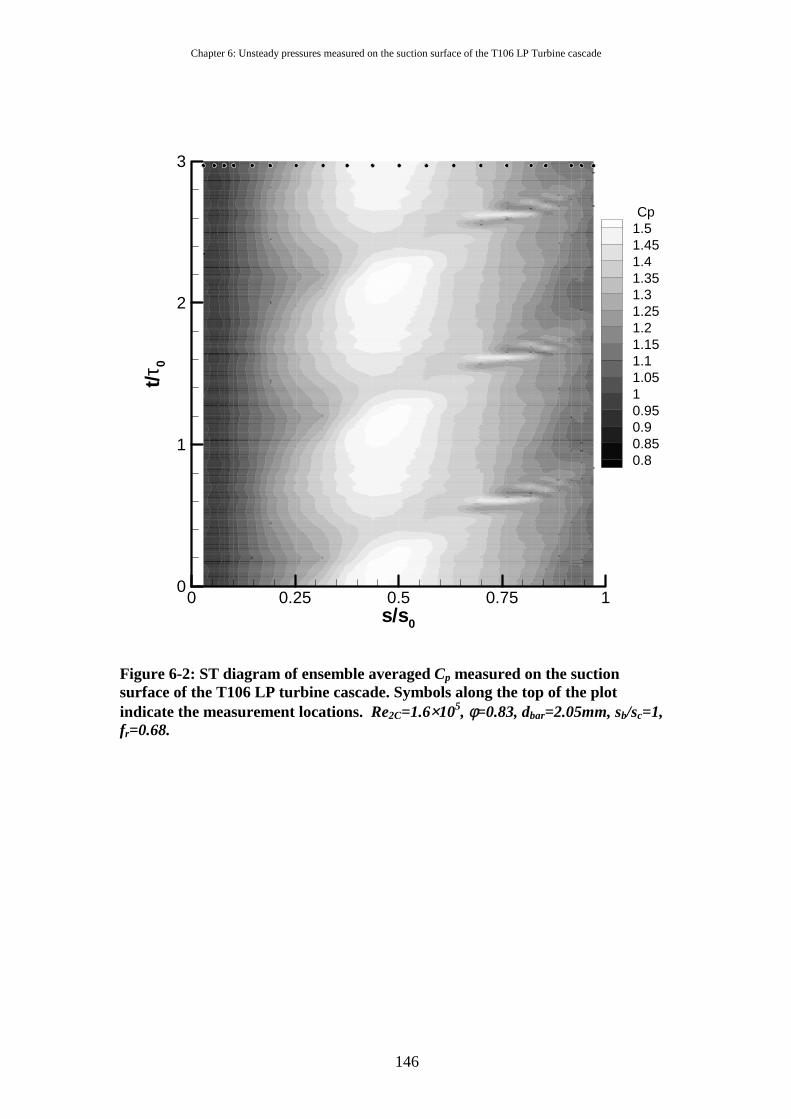
Chapter 6: Unsteady pressures measured on the suction surface of the T106 LP Turbine cascade
146
s/s0
t/τ 0
0 0.25 0.5 0.75 10
1
2
3
Cp1.51.451.41.351.31.251.21.151.11.0510.950.90.850.8
Figure 6-2: ST diagram of ensemble averaged Cp measured on the suction surface of the T106 LP turbine cascade. Symbols along the top of the plot indicate the measurement locations. Re2C=1.6×10⁵, φ=0.83, dbar=2.05mm, sb/sc=1, fr=0.68.
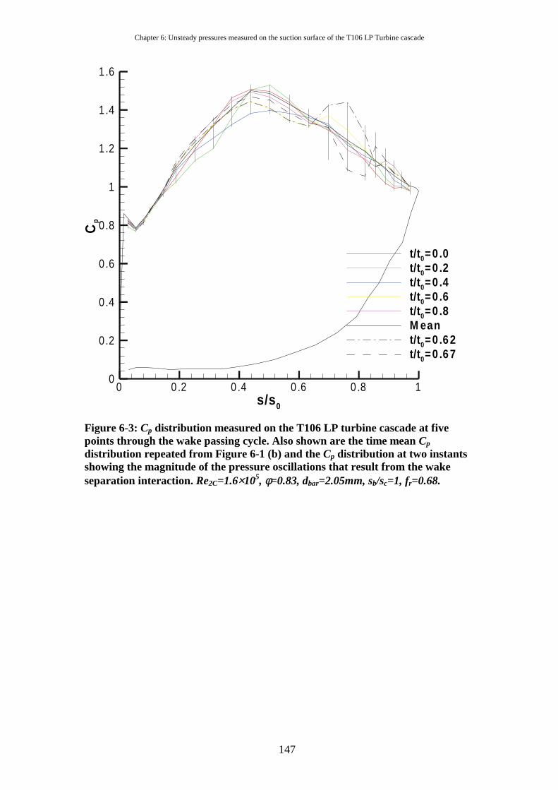
Chapter 6: Unsteady pressures measured on the suction surface of the T106 LP Turbine cascade
147
s/s 0
Cp
0 0 .2 0 .4 0 .6 0 .8 10
0.2
0.4
0.6
0.8
1
1.2
1.4
1.6
t/t 0=0 .0t/t 0=0 .2t/t 0=0 .4t/t 0=0 .6t/t 0=0 .8M eant/t 0=0 .6 2t/t 0=0 .6 7
Figure 6-3: Cp distribution measured on the T106 LP turbine cascade at five points through the wake passing cycle. Also shown are the time mean Cp distribution repeated from Figure 6-1 (b) and the Cp distribution at two instants showing the magnitude of the pressure oscillations that result from the wake separation interaction. Re2C=1.6×10⁵, φ=0.83, dbar=2.05mm, sb/sc=1, fr=0.68.
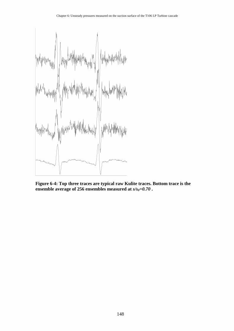
Chapter 6: Unsteady pressures measured on the suction surface of the T106 LP Turbine cascade
148
Figure 6-4: Top three traces are typical raw Kulite traces. Bottom trace is the ensemble average of 256 ensembles measured at s/s0=0.70 .
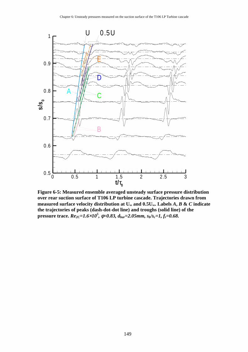
Chapter 6: Unsteady pressures measured on the suction surface of the T106 LP Turbine cascade
149
t/τ0
s/s 0
0 0 .5 1 1 .5 2 2 .5 30.5
0.6
0.7
0.8
0.9
1
C
D
E
0.5UU
A
B
Figure 6-5: Measured ensemble averaged unsteady surface pressure distribution over rear suction surface of T106 LP turbine cascade. Trajectories drawn from measured surface velocity distribution at U∞ and 0.5U∞. Labels A, B & C indicate the trajectories of peaks (dash-dot-dot line) and troughs (solid line) of the pressure trace. Re2C=1.6×10⁵, φ=0.83, dbar=2.05mm, sb/sc=1, fr=0.68.
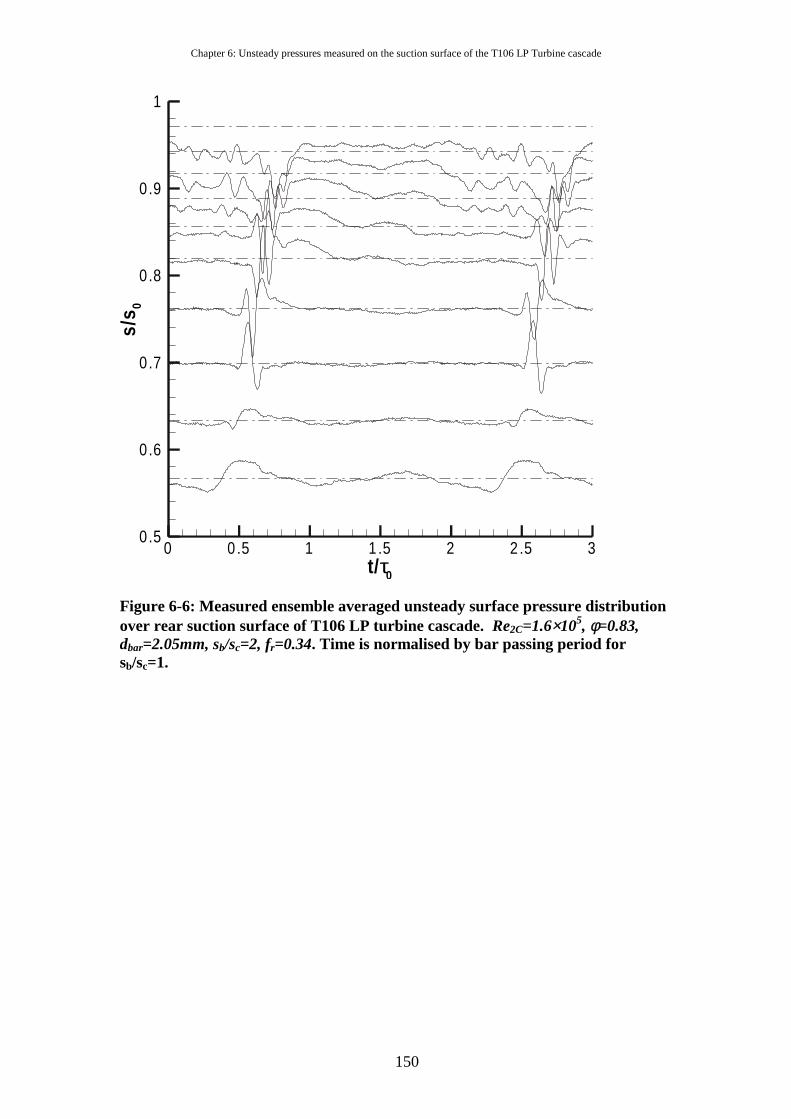
Chapter 6: Unsteady pressures measured on the suction surface of the T106 LP Turbine cascade
150
t/τ0
s/s 0
0 0 .5 1 1 .5 2 2 .5 30.5
0.6
0.7
0.8
0.9
1
Figure 6-6: Measured ensemble averaged unsteady surface pressure distribution over rear suction surface of T106 LP turbine cascade. Re2C=1.6×10⁵, φ=0.83, dbar=2.05mm, sb/sc=2, fr=0.34. Time is normalised by bar passing period for sb/sc=1.
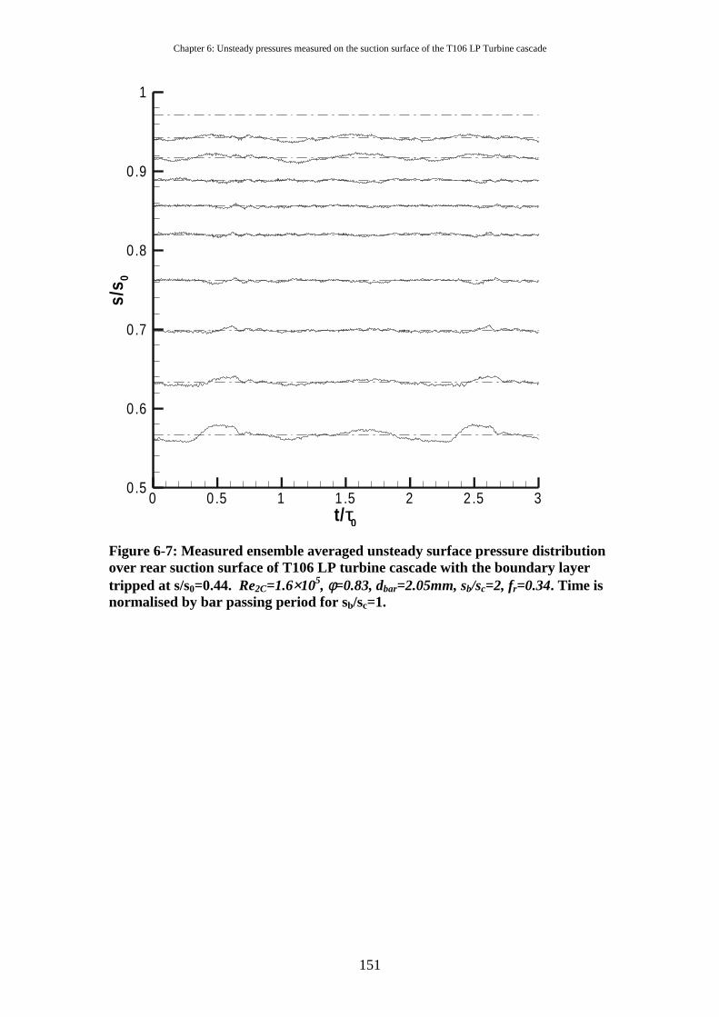
Chapter 6: Unsteady pressures measured on the suction surface of the T106 LP Turbine cascade
151
t/τ0
s/s 0
0 0 .5 1 1 .5 2 2 .5 30.5
0.6
0.7
0.8
0.9
1
Figure 6-7: Measured ensemble averaged unsteady surface pressure distribution over rear suction surface of T106 LP turbine cascade with the boundary layer tripped at s/s0=0.44. Re2C=1.6×10⁵, φ=0.83, dbar=2.05mm, sb/sc=2, fr=0.34. Time is normalised by bar passing period for sb/sc=1.
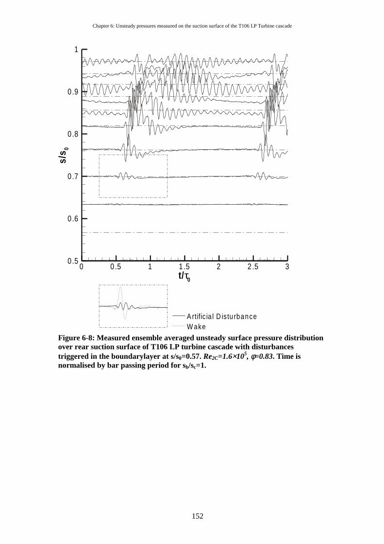
Chapter 6: Unsteady pressures measured on the suction surface of the T106 LP Turbine cascade
152
t/τ0
s/s 0
0 0 .5 1 1 .5 2 2 .5 30.5
0.6
0.7
0.8
0.9
1
A rtific ia l D is tu rbanceW ake
Figure 6-8: Measured ensemble averaged unsteady surface pressure distribution over rear suction surface of T106 LP turbine cascade with disturbances triggered in the boundarylayer at s/s0=0.57. Re2C=1.6×10⁵, φ=0.83. Time is normalised by bar passing period for sb/sc=1.
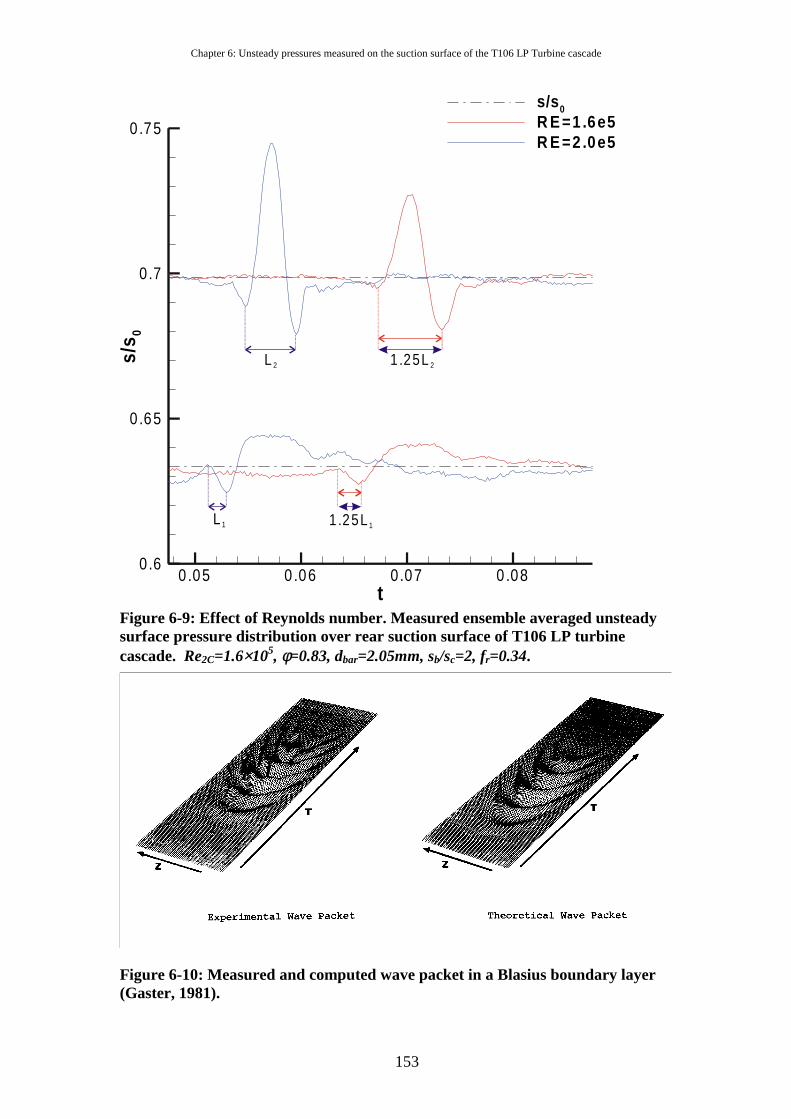
Chapter 6: Unsteady pressures measured on the suction surface of the T106 LP Turbine cascade
153
t
s/s 0
0 .05 0 .06 0.07 0 .080.6
0 .65
0.7
0 .75
s/s 0R E =1 .6e5R E =2 .0e5
L 2 1 .25L 2
L 1 1 .25L 1
Figure 6-9: Effect of Reynolds number. Measured ensemble averaged unsteady surface pressure distribution over rear suction surface of T106 LP turbine cascade. Re2C=1.6×10⁵, φ=0.83, dbar=2.05mm, sb/sc=2, fr=0.34.
Figure 6-10: Measured and computed wave packet in a Blasius boundary layer (Gaster, 1981).
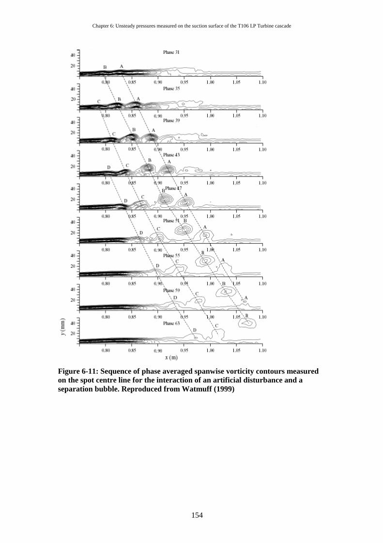
Chapter 6: Unsteady pressures measured on the suction surface of the T106 LP Turbine cascade
154
Figure 6-11: Sequence of phase averaged spanwise vorticity contours measured on the spot centre line for the interaction of an artificial disturbance and a separation bubble. Reproduced from Watmuff (1999)
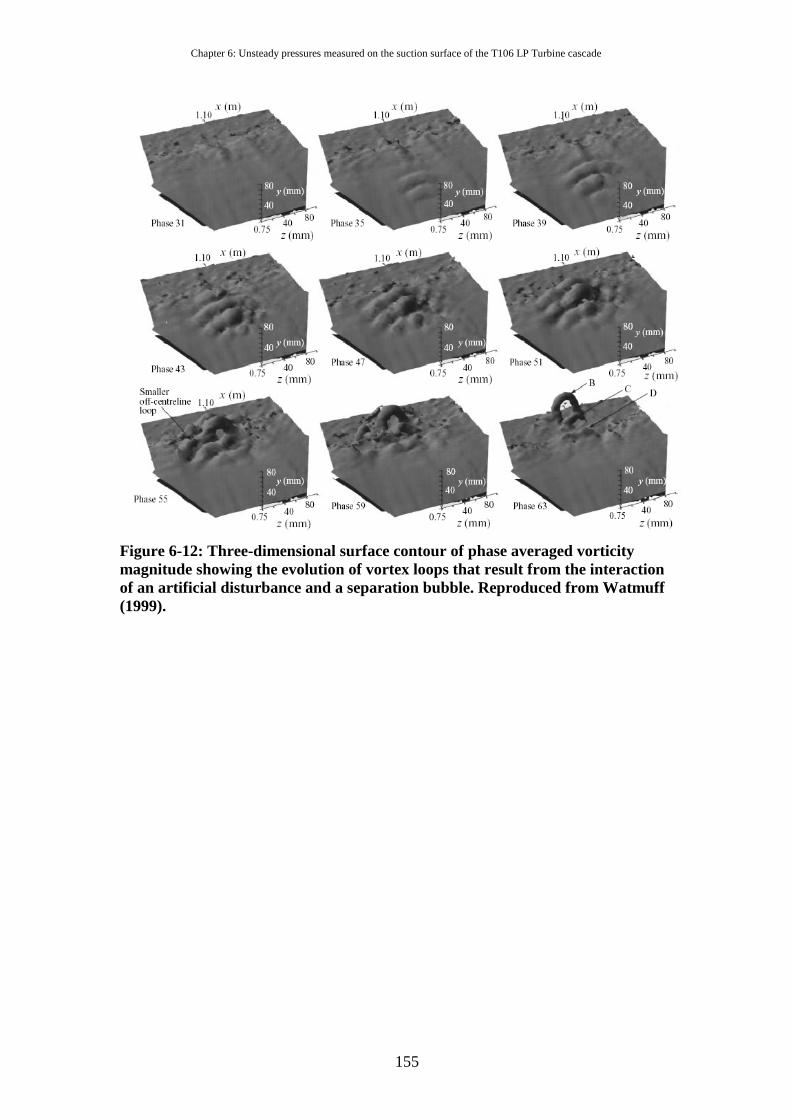
Chapter 6: Unsteady pressures measured on the suction surface of the T106 LP Turbine cascade
155
Figure 6-12: Three-dimensional surface contour of phase averaged vorticity magnitude showing the evolution of vortex loops that result from the interaction of an artificial disturbance and a separation bubble. Reproduced from Watmuff (1999).
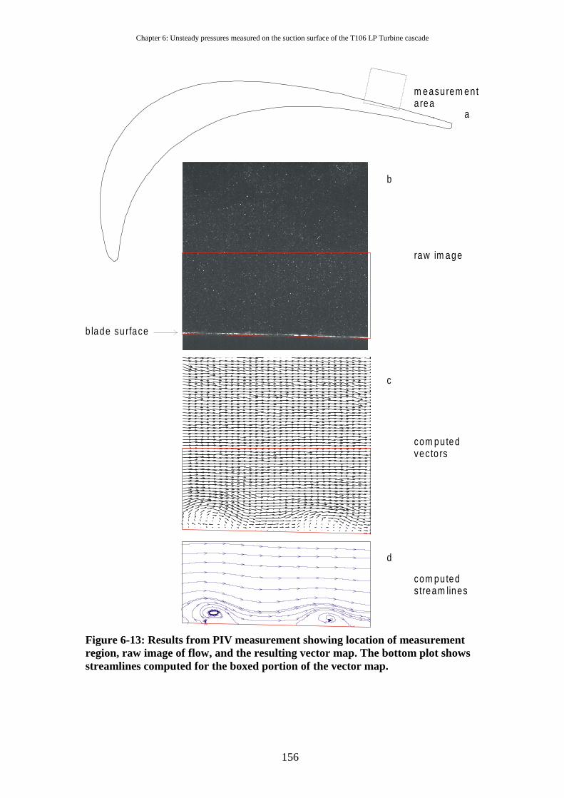
Chapter 6: Unsteady pressures measured on the suction surface of the T106 LP Turbine cascade
156
raw im age
m easurem enta rea
com puted vec to rs
com puted s tream lines
b lade su rface
a
b
c
d
Figure 6-13: Results from PIV measurement showing location of measurement region, raw image of flow, and the resulting vector map. The bottom plot shows streamlines computed for the boxed portion of the vector map.
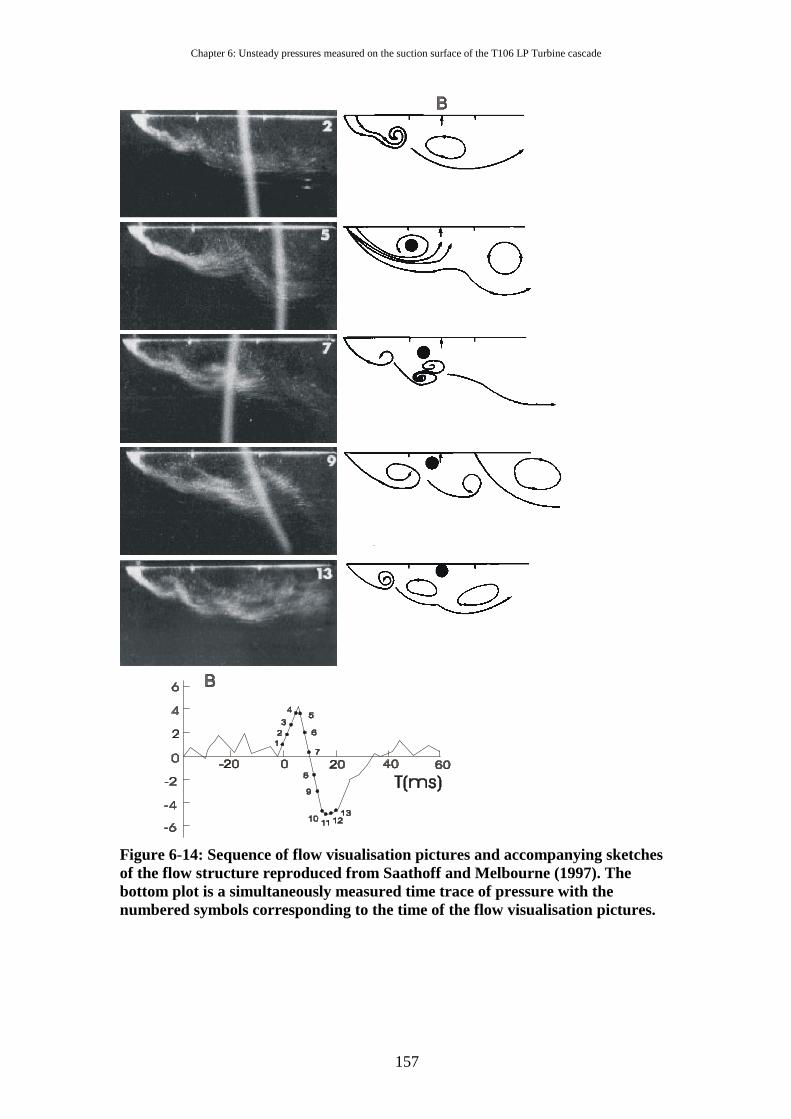
Chapter 6: Unsteady pressures measured on the suction surface of the T106 LP Turbine cascade
157
Figure 6-14: Sequence of flow visualisation pictures and accompanying sketches of the flow structure reproduced from Saathoff and Melbourne (1997). The bottom plot is a simultaneously measured time trace of pressure with the numbered symbols corresponding to the time of the flow visualisation pictures.
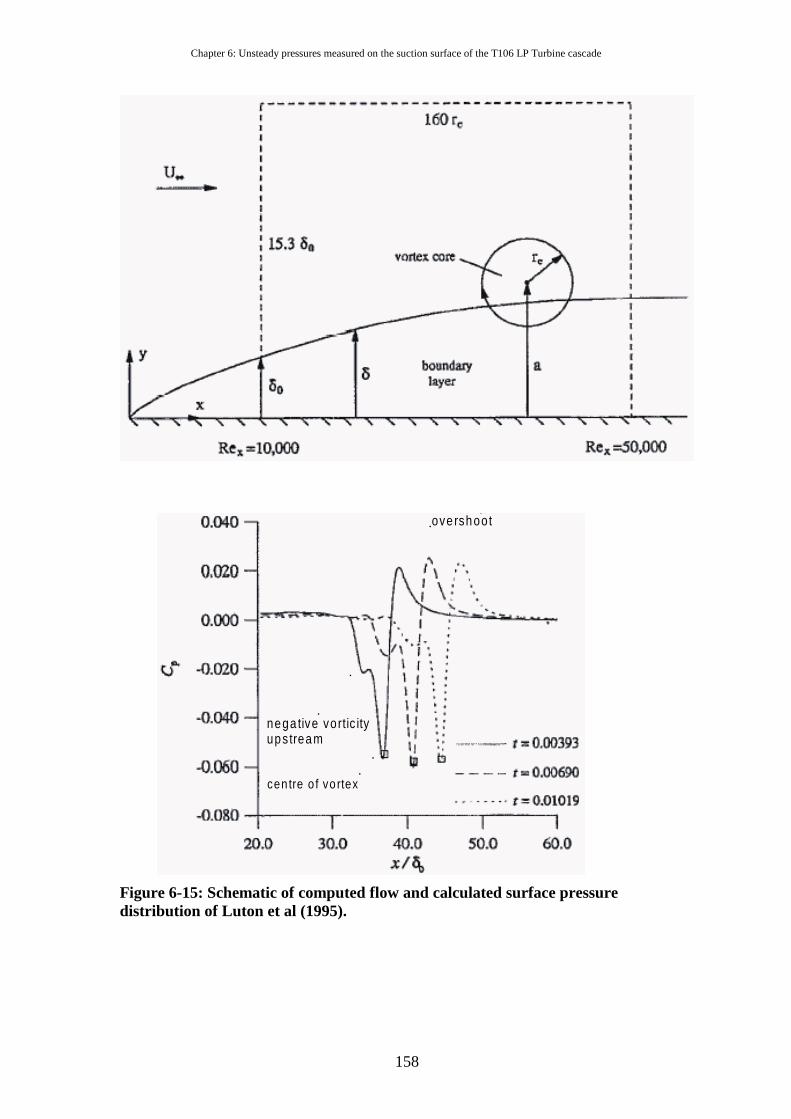
Chapter 6: Unsteady pressures measured on the suction surface of the T106 LP Turbine cascade
158
cen tre o f vo rtex
ove rshoot
nega tive vortic ityups tream
Figure 6-15: Schematic of computed flow and calculated surface pressure distribution of Luton et al (1995).
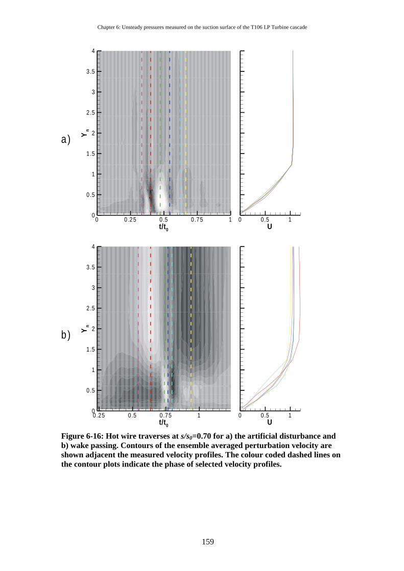
Chapter 6: Unsteady pressures measured on the suction surface of the T106 LP Turbine cascade
159
t/t 0
Yn
0 0.25 0.5 0 .75 10
0.5
1
1.5
2
2.5
3
3.5
4
U0 0.5 1
a )
b)
U0 0.5 1
t/t 0
Yn
0.25 0.5 0 .75 10
0.5
1
1.5
2
2.5
3
3.5
4
Figure 6-16: Hot wire traverses at s/s0=0.70 for a) the artificial disturbance and b) wake passing. Contours of the ensemble averaged perturbation velocity are shown adjacent the measured velocity profiles. The colour coded dashed lines on the contour plots indicate the phase of selected velocity profiles.
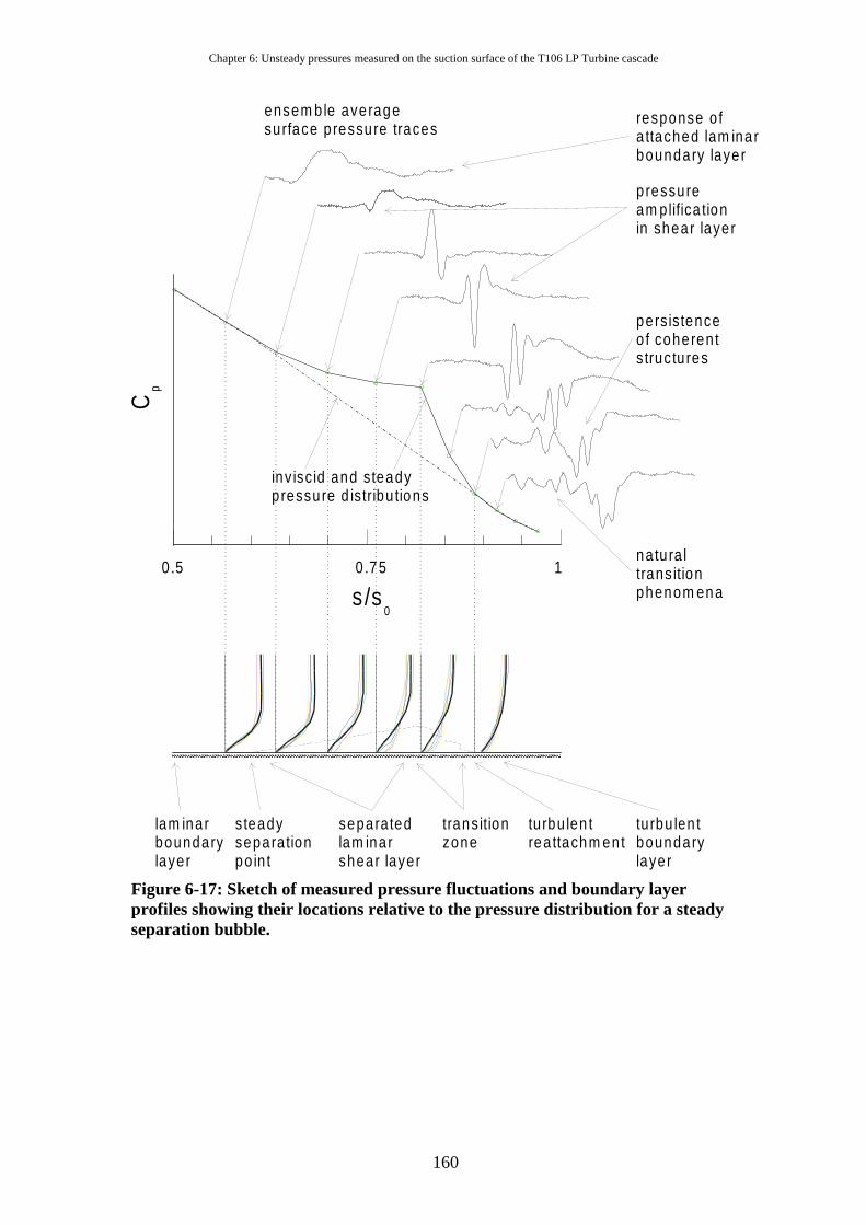
Chapter 6: Unsteady pressures measured on the suction surface of the T106 LP Turbine cascade
160
0.5 0 .75 1
s /s0
Cp
s teadyseparationpo in t
separatedlam inarshear layer
trans itionzone
turbu len trea ttachm ent
ensem ble averagesurface p ressure traces
inv isc id and steadypressure d istribu tions
lam inarboundarylayer
turbu len tboundarylayer
na tu ra ltrans itionphenom ena
pressuream plifica tion in shear layer
response o fa ttached lam inarboundary layer
pers istenceo f coheren t s truc tu res
Figure 6-17: Sketch of measured pressure fluctuations and boundary layer profiles showing their locations relative to the pressure distribution for a steady separation bubble.
161
Chapter 7: Boundary layer measurements on the T106 LP turbine cascade
7.1 Introduction The large amplitude unsteady surface pressure fluctuations that were presented
in Chapter 6 represent a newly discovered aspect of wake boundary layer interaction.
In order to gain a better understanding of this interaction and the cause of the large
amplitude pressure fluctuations, a series of boundary layer traverses were performed
using 2D LDA.
The results, presented as S-T diagrams of the boundary layer measurements,
provide a new insight into the wake-induced transition mechanisms found on LP
turbine blades with inflexional boundary layer profiles associated with separation
bubbles. The traditional wake-induced bypass transition path lags the passing of the
wake in the freestream, however, when the wake passes over regions of inflexional
boundary layer profiles, the traditional bypass transition is preceded by an interaction
that occurs immediately beneath the passing wake. Coherent structures resulting from
this interaction are identified on the S-T diagrams.
The boundary layer state is then investigated at three representative phases
during the wake passing cycle and this identifies the coherent structures to be vortices
embedded in the boundary layer that are formed as the wake passes over regions of
inflexional profiles. The production and dissipation of turbulent kinetic energy (TKE)
calculated from the LDA measurements show that these vortices are regions of very
high production and dissipation of TKE within the boundary layer.
Finally, a detailed view of the shear layer breakdown induced by the passing
wake is presented. A cat’s eye pattern is identified in the measured vorticity contours
of the separated shear layer and this provides evidence that the breakdown of the
separated shear layer is by an inviscid Kelvin-Helmholtz mechanism that results in the
formation of rollup vortices.
7.2 Details of 2D LDA boundary layer measurements A series of boundary layer traverses were performed on the suction surface of
the T106 LP turbine cascade. The measurement grid is shown in Figure 7-1. Each
traverse was performed perpendicular to the local blade surface. The blade was
painted matt black to minimise reflections from the intersecting laser beams except
Chapter 7: Boundary layer measurements on the T106 LP turbine cascade
162
for a strip at midspan, which was left unpainted to avoid contamination of the static
pressure tappings. For this reason the traverses were performed at 45% span as in
Chapter 5. The first traverse point was 0.1mm from the blade surface and the first 16
points were exponentially distributed within the boundary layer. The final 4 of the 20
traverse points were evenly spaced from the boundary layer edge to a point 16mm
from the blade surface. In the streamwise direction 25 measurement locations were
used. These were selected based on previous measurements.
The Reynolds number based on chord and time mean isentropic exit velocity
was Re2C=1.6×10⁵ and the flow coefficient was φ=0.83. The bar pitch matched the
cascade pitch so that sb/sc=1 (fr=0.68). This flow condition matches those presented in
Chapter 5 and Chapter 6. Ensemble averaging of the LDA data was performed as
described in Chapter 3.
7.3 Wake induced transition schematic for LP turbines The transition process occurring on LP turbine blades is multi-modal and
unsteady. Although described by a number of authors (e.g. Mayle (1991), Walker
(1993), Addison and Hodson (1992), Schulte (1995)), perhaps the most
comprehensive study is that of Halstead et al (1997 a-d). To facilitate their description
of the boundary layer development, they presented S-T diagrams as schematics
highlighting the boundary layer state during the wake-induced transition. The same
approach is adopted here.
Two schematics are presented. Firstly, the traditional view of wake-induced
transition for attached boundary layers on LP turbine blades is presented. Then the
wake-induced transition process involving the interaction of the wake and the
inflexional boundary layer profiles associated with a separation bubble is shown. The
experimental basis of the second schematic follows in §7.4 .
7.3.1 A traditional schematic of wake induced transition Following the description of Halstead et al (1997 a), two generic transition
paths may be identified on the blade surface. The wake-induced path, labelled 1 in the
schematic of Figure 7-2, arises when the turbulent wake from an upstream bladerow
washes over the blade surface. High levels of turbulence convect with the wake in the
freestream, the trajectory of which is denoted by line 3. The wake turbulence diffuses
into the boundary layer, which then undergoes a bypass transition. This bypass
Chapter 7: Boundary layer measurements on the T106 LP turbine cascade
163
transition is initiated by a transitional region where isolated turbulent spots may
intermittently form, prior to their merging into the wake-induced turbulent strip. The
wake-induced bypass transition happens along trajectory line 4 and lags behind the
trajectory of the wake in the freestream. This was observed in the measurements
presented in Chapter 4. The turbulent strip resulting from the wake-induced transition
describes a wedge shape on the S-T diagram due to the trailing edges of the turbulent
strip convecting slower than the leading edge. The elevated turbulence of the wake
causes the wake-induced bypass transition to occur nearer to the leading edge than the
undisturbed transition location. The wake induced and natural transition locations are
marked on Figure 7-2.
The transition path between the wakes is labelled 2 in Figure 7-2 and is
characterised by the calmed region and a natural transition process. After the wake
has passed, the stimulus for early transition is removed and the turbulent boundary
layer upstream of the natural transition location relaxes to its pre-transition state. This
relaxation process results in the calmed region, which is characterised by low levels of
dissipation and full velocity profiles that suppress boundary layer separation. The
calmed region spreads as it convects downstream due to the different convection
velocities for the trailing edge of turbulent spots and the trailing edge of the clamed
region. After the influence of the clamed region has decayed, the blade surface
boundary layer undergoes natural transition, which for LP turbines at cruise condition
may be incomplete at the trailing edge.
7.3.2 Schematic of wake-induced transition with inflexional boundary layer profiles
A schematic for the transition process resulting from the interaction of a
turbulent wake and the inflexional profiles of a separating boundary layer is shown in
Figure 7-3. As before the wake induced path is labelled 1, and the path between the
wakes is labelled 2.
In Chapter 6 it was shown that the interaction of the wake and the inflexional
boundary layer profiles resulted in rollup vortices being formed. These rollup vortices
were found to form as the wake passed over the region where a separation bubble
formed in the absence of wakes. Further evidence of this is presented in §7.4 .
In Figure 7-3, the wake-induced path, labelled 1, differs to that in Figure 7-2.
There is no lag between the wake passing in the freestream (trajectory line 3) and the
Chapter 7: Boundary layer measurements on the T106 LP turbine cascade
164
response of the boundary layer. The rollup of vortices resulting from the interaction of
the wake and inflexional profiles occurs by an inviscid mechanism. The diffusion of
turbulence into the boundary layer is thus not a necessary precursor to the rollup of
the shear layer and thus there is no time lag between the wake passing and the
boundary layer response. The inviscid interaction resulting in the formation of roll-up
vortices is represented in the schematic of Figure 7-3 as a series of wedges originating
beneath the centre of the wake. The rollup vortices break down and a region of
turbulent boundary layer follows the inviscid rollup process.
After the inviscid interaction of the wake and the inflexional profiles, the wake
turbulence diffuses into the boundary layer and induces a bypass transition as
described in §7.3.1 above. This bypass transition is indicated in the schematic of
Figure 7-3 by the wake-induced transitional and turbulent strips occurring along
trajectory 4.
The transition path between the wakes is labelled 2 and is initially controlled
by the calmed region that follows the wake induced turbulent strip. However, after the
influence of the calming has passed, the boundary layer profiles become inflexional
and begin to separate under the strong adverse pressure gradient. The trailing edge of
this inflexional region initially follows the trajectory of the trailing edge of the calmed
region. Thereafter, the inflexional or separating flow undergoes transition, however,
as shown in Chapter 4, this is not the highly dissipative transition process associated
with separation bubbles found in steady flows. Immediately prior to the arrival of the
wake, the separation location is observed to move fractionally upstream. This is the
influence of the negative jet, which alters the pressure gradient locally and is a
precursor to the inviscid rollup occurring beneath the wake.
7.4 An S-T view of the measured boundary layer The measurements supporting the schematic of wake-induced transition with
inflexional boundary layer profiles is now presented. The 2D LDA boundary layer
traverse data is presented in S-T diagrams in Figure 7-4 to Figure 7-8. To aid
visualisation of the unsteady process the data is copied onto three wake passing
periods as it was in Chapter 4.
Chapter 7: Boundary layer measurements on the T106 LP turbine cascade
165
7.4.1 Boundary Layer Edge Velocity The boundary layer edge is defined as the wall normal distance where the
velocity is 98% of the maximum velocity measured in the ensemble-average profile at
that location and time. The velocity at this point is the boundary layer edge velocity,
measurements of which are plotted as an S-T diagram in Figure 7-4. Three trajectory
lines denoted A, B and E, are drawn at the time average boundary layer edge velocity.
Line A marks the peak velocity due to the negative jet of the approaching wake. Line
B is approximately at the centre of the wake. Line E marks the minimum velocity,
which occurs after the negative jet of the wake has passed.
Two further lines, labelled C and D, are drawn to mark two distinct features
originating along the wake centre at s/s0≈0.70 and s/s0≈0.80. These perturbations to
the boundary layer edge velocity have not previously been observed. They are
attributed to the rollup vortices that form as the wake interacts with the inflexional
boundary layer as described in Chapter 6. The rollup vortices can be seen to follow
trajectories slower than the local freestream. Indeed, dashed lines C and D are drawn
with a trajectory of half the freestream velocity. The vortex closer to the leading edge
initially convects more slowly than this. These observations are in agreement with the
findings of Chapter 6.
7.4.2 TKE thickness Due to practical constraints, the boundary layer state on turbomachinery
blading is typically inferred from measurements made with hot-film anemometers.
The results are thus qualitative, however, it is not the quasi-shear stress, but rather the
random unsteadiness (ensemble average RMS), which is used to indicate the
boundary layer state. This is possible as transitional and turbulent boundary layers
have far higher levels of random unsteadiness than laminar boundary layers.
D’Ovidio et al (2001 b) sought to recover the familiarity of using RMS as an
indicator of boundary layer state while using all the data from hot wire boundary layer
traverses. They made use of the Blackwelder parameter, which was defined as the
integral of the RMS velocity through the boundary layer thickness non-
dimensionalised by the time average displacement thickness. A similar approach is
adopted for the current measurements. The parameter δ’ is defined as the integral of
TKE through the boundary layer. Thus
Chapter 7: Boundary layer measurements on the T106 LP turbine cascade
166
∫=
+=98
0
2221
2
98
, )''(1
δ
δy
dyvuU
( 7-1)
An S-T diagram of δ’ is shown in Figure 7-5. The trajectory lines and labels are
copied from Figure 7-4.
Upstream of s/s0=0.70, δ’ is low throughout the wake passing cycle. In this
region, the boundary layer is laminar and is not significantly influenced by the passing
wakes.
Downstream of s/s0=0.70, the wake-induced path is characterised by very high
levels of δ’ . The onset of elevated δ’ lies along the wake centre at line B and does not
lag behind the wake. The lack of a lag time corresponds to the region where the rollup
vortices were observed in Figure 7-4 at labels C and D. This provides experimental
evidence that the inviscid rollup occurs at the wake centre and does not lag behind the
passing wake. The coherent rollup vortices follow trajectories of approximately 0.5U∞
before merging into a region of high δ’ that persists to the trailing edge.
A second strip of elevated δ’ is seen to originate at label H. This strip lags
behind the passing of the wake and is a result of a wake-induced bypass transition.
Also shown in Figure 7-5 is line F drawn with a trajectory of 0.5U∞ and line G drawn
with a trajectory of 0.3U∞. These lines, drawn from the trailing edge of the wake
induced turbulent strip, mark the trajectory of the trailing edge of turbulent spots and
the trailing edge of the calmed region respectively.
At the traverse location closest to the trailing edge, four distinct levels of δ’
are distinguishable. The highest levels occur between lines B and E and originate from
the interaction of the wake and the inflexional profiles of the separating boundary
layer. The next highest region of δ’ occurs between lines E and F and results from the
turbulent strip formed by the wake induced bypass transition. The lowest region of δ’
occurs between lines F and G. This region corresponds to the calmed region and
shows that the calmed region persists to the trailing edge. Finally between G and A of
the following cycle the level of δ’ is again elevated due to the natural transition that
occurs once the influence of the calmed region has passed.

Chapter 7: Boundary layer measurements on the T106 LP turbine cascade
167
7.4.3 Integral Parameters The ensemble average integral parameters were calculated from the measured
velocity profiles. The displacement thickness, δ*, and momentum thickness, θ, are
presented in Figure 7-6 and Figure 7-7 respectively. Figure 7-8 presents an S-T
diagram of the boundary layer shape factor, H12. Trajectory lines and labels are
repeated from previous S-T diagrams.
The rollup vortices labelled C and D change the boundary layer profiles and
thus affect the integral parameters. A close inspection of Figure 7-6 reveals that in the
region of the rollup vortices a series of peaks and troughs of δ* are formed. The
trajectories C and D lie along regions of reduced δ* while between these trajectories
regions of elevated δ* are measured. However, Figure 7-7 reveals generally elevated
levels of θ with no distinct features. The rollup vortices thus influence δ* more than θ.
This is highlighted in Figure 7-8 where trajectories C and D lie in distinct wedge
shaped regions of reduced H12 protruding into the elevated H12 of the inflexional flow.
In Figure 7-7, two regions of elevated θ are identified. The first, originating at
C, is due to the turbulent boundary layer that results from the breakdown of the rollup
vortices. The second region of elevated θ is seen to form at label H. This corresponds
to the second region of elevated δ'’ that was previously identified to result from the
wake-induced bypass transition in Figure 7-5.
A region of calmed flow bounded by lines F and G follows the wake induced
turbulent strip. The calming is associated with low levels of δ* and θ observed in this
region. The reduced θ region is seen to persist to the trailing edge and identifies the
calmed region with low losses as shown by Howell (1999). After the calmed region
has passed, both δ* and θ increase gradually. In this region H12 increases as δ*
increases more rapidly than θ. This describes the process whereby the calmed
boundary layer relaxes back to the inflexional profiles and a separating boundary
layer under a strong adverse pressure gradient.
The effect of the wake’s negative jet on the boundary layer is apparent
between lines A and B. As the wake approaches θ decreases while δ* is unaffected.
The result of this is to produce more inflexional boundary layer profiles with
increased H12. The separation point thus moves marginally upstream.

Chapter 7: Boundary layer measurements on the T106 LP turbine cascade
168
The values of θ at the blade trailing edge were used by Howell (1999) to
compare the boundary layer losses at different phases through the wake passing cycle.
Between lines B and E, the trailing edge momentum thickness is highest. The S-T
diagram shows that this region of high θ is the turbulent fluid that results from the
breakdown of the rollup vortices formed due to the inviscid interaction of the wake
and the separation bubble. A second region of high θ at the trailing edge occurs
between lines E and F. This results from the turbulent spots formed by the wake
induced bypass transition. These observations show the same character as those made
from the trailing edge levels of δ’ .
7.5 Unsteady boundary layer development Further details of the 2D LDA boundary layer traverses are presented to gain a
better understanding of the interaction of the wake and separating boundary layer. To
achieve this understanding, a series of phases through the wake passing cycle were
selected for analysis.
A collage of the mean and turbulent flow quantities measured through the
boundary layer at each of these selected phases are presented in Figure 7-10 to Figure
7-13. The mean flow is described by vector plots of the mean and perturbation
velocities and a contour plot of vorticity calculated from the measured velocity field.
The mean velocity vectors show the boundary layer profile and character while the
perturbation velocity vectors highlight the unsteady components of the velocity field,
in particular, the wall normal velocity components and the position of the wake. Plots
of vorticity enable the identification of vortical structures embedded in the sheared
fluid of the boundary layer. Further information about the nature of the boundary
layer profiles is also available as the peaks of vorticity away from the wall highlight
the inflexional profiles and free shear layers.
Contour plots of the ensemble average turbulent quantities are also presented
at each of the selected phases. The turbulent kinetic energy (TKE) is calculated
directly from the measured velocity fluctuations. The production of TKE is calculated
from the measured Reynolds stresses and mean velocity gradients as in Chapter 5.
Finally, the dissipation of TKE is presented. This was calculated simply as the
difference in TKE flux and TKE production. Details of the calculation of the
dissipation of TKE are described in Appendix III.
Chapter 7: Boundary layer measurements on the T106 LP turbine cascade
169
Figure 7-9 shows the selected phases superimposed on the S-T schematic of
wake induced transition with a separating boundary layer that was presented in Figure
7-3. Phases i, ii and iii are equally spaced through the inviscid interaction with i just
prior to the interaction. The sequence depicts the rollup of the separated shear layer
induced by the wake passing. Phase iv is near the end of the calmed region and
depicts the boundary layer state between wakes.
7.5.1 Boundary layer state before the interaction of the wake and inflexional profiles
The boundary layer state at phase i can be inferred from the schematic of
Figure 7-9. Upstream of the separation point, 1, the boundary layer is laminar and
attached while downstream of 1 the boundary layer profiles are inflexional. The
separating boundary layer undergoes transition from point 2 and reattaches at position
3. The position of the wake in the freestream is immediately upstream of the
separation point, 1. These labels are transferred to the collage of boundary layer
measurements at phase i which is presented in Figure 7-10.
Figure 7-10 (a) shows the ensemble average velocity vectors at phase i. The
inflexional profiles of the separating boundary layer are evident in the region between
1 and 2. These inflexional profiles have their maximum vorticity levels displaced
from the wall (Figure 7-10 (c)), which is indicative of a free shear layer between 1
and 2. At this phase, the shear layer is not perturbed. This is confirmed by the absence
of wall normal components of the perturbation velocity vectors in Figure 7-10 (b).
Also evident from Figure 7-10 (b) is the position of the wake, the centre of which is
located immediately upstream of 1 and is marked by a filled circle.
The reattachment process that results from the transition of the inflexional
profiles occurs between 2 and 3. This region is characterised by the velocity profiles
becoming fuller and turbulent in character. In the vorticity contour plots, this process
is characterised by the disappearance of the peak displaced from the wall and by
reduced levels of vorticity in the outer boundary layer as the profiles become fuller
and more turbulent.
The transition associated with the free shear layer is accompanied by increased
levels of TKE. This increase in TKE is seen to start at 2 in Figure 7-10 (d) and extend
to the trailing edge. The increased levels of TKE coincide with increased levels of
production and dissipation of TKE as shown by Figure 7-10 (e) and (f). The velocity
Chapter 7: Boundary layer measurements on the T106 LP turbine cascade
170
profiles downstream of 3 are full and so the velocity gradients are low. The TKE
production thus results primarily from increased levels of Reynolds stresses in the
turbulent boundary layer. The dissipation and production are of similar levels and
occur at the same location, however, the reduced streamwise resolution compromises
the quality of the measurements in this region.
7.5.2 Interaction of wake and inflexional boundary layer It was shown in Chapter 6 that the inviscid rollup of the separated shear layer
is triggered by the wake passing. The schematic of Figure 7-9 shows that the
boundary layer at phase ii is representative of this inviscid rollup. The interaction of
the wake and inflexional profiles occurs between 4 and 6. Downstream of 6 the
boundary layer is still inflexional as the wake has not yet reached this location. The
transition and reattachment of the inflexional profiles occurs between 7 and 8. These
labels have been transferred to Figure 7-11, which presents the boundary layer state
measured at this phase.
The mean velocity profiles of Figure 7-11 (a) differ from those at phase i. At 4
the profiles are inflexional and this is confirmed by the vorticity contours in Figure
7-11 (c) which show a peak detached from the wall. However, between 4 and 5, the
velocity profiles are full and at 5 the profiles are again inflexional. Between 5 and 6
the profiles are again full while at 6 the profiles are again inflexional. This rapid
change with distance along the blade surface is attributed to the rollup of the shear
layer induced by the wake. Indeed, rollup vortices may be identified at 4, 5 & 6 in
Figure 7-11 (c) as regions of high vorticity embedded within the boundary layer. The
boundary layer edge can be inferred from the edge of the elevated vorticity region.
From this the rollup vortices can be seen to thicken the boundary layer locally,
particularly at 5. This was also observed in the S-T diagram of δ* shown in Figure
7-8. The perturbation velocity vectors of Figure 7-11 (b) show significant wall normal
velocities associated with the rollup vortices. The rollup vortex with its centre at 5
may be identified in the perturbation velocity vectors. It is clear that the rollup vortex
at 5 induces large local flow curvature and it is this flow curvature that is responsible
for the large pressure oscillations measured at the wall in Chapter 6.
Downstream of the wake, between 6 and 7, the velocity profiles are inflexional
and the vorticity contours show a peak detached from the wall. This region has not yet

Chapter 7: Boundary layer measurements on the T106 LP turbine cascade
171
been affected by the wake passing. The transition and reattachment of the inflexional
profiles between 7 and 8 occurs as in phase i.
Figure 7-11 (d) shows contours of TKE at phase ii. The elevated turbulence
associated with the wake (see contour level 0.001) can be seen to extend from 4 to the
trailing edge and the boundary layer TKE is elevated throughout this region. Three
regions of elevated TKE are distinguishable at labels 4,5 & 6 and correspond to the
centres of the rollup vortices previously identified. The highest levels of TKE are
located at 5 which is the largest and most distinct of the rollup vortices. The reduced
levels of TKE at 7 corresponds to the inflexional profiles that have not yet interacted
with the wake. Downstream of this, the elevated TKE is a result of the natural
transition of the inflexional profiles.
The production and dissipation of TKE are presented in Figure 7-11 (e)&(f).
These follow the distribution of TKE with elevated production and elevated
dissipation at the centre of the vortices at 4, 5 & 6. The peak levels of production and
the peak levels of dissipation are located at the centre of the vortex at 5. The natural
transition downstream of 8 is also associated with elevated levels of TKE production
and dissipation. In this region, the dissipation extends further from the wall then the
production.
7.5.3 Boundary layer after wake interaction From Figure 7-9, it can be seen that at phase iii the boundary layer is
dominated by the wake induced turbulent strip. The wake-induced strip can be further
decomposed into three regions. Between 9 and 10, the boundary layer is transitional,
between 10 and 11 the boundary layer is turbulent due to the wake induced bypass
transition and downstream of 11 the boundary layer is turbulent as a result of the
breakdown of the rollup vortices formed by the interaction of wake and the
inflexional profiles. These labels are transferred to Figure 7-12.
The mean velocity profiles are shown in Figure 7-12 (a). Upstream of 9 the
boundary layer profiles are laminar. Between 9 and 10 the boundary layer profiles
have the shape of attached laminar profiles but the levels of TKE in this region are
elevated (see Figure 7-12 (d)). This indicates that the profiles are transitional in this
region.
Chapter 7: Boundary layer measurements on the T106 LP turbine cascade
172
Downstream of 10 the velocity profiles have a turbulent shape. However, the
levels of TKE downstream of 11 are far higher than between 10 and 11. This is
attributed to the breakdown of the rollup vortices. An isolated region of elevated TKE
can be identified in Figure 7-12 (d) at 11. Although not evident in the vorticity
contours, this is attributed to a rollup vortex and is accompanied by elevated
production and elevated dissipation that accompanied the rollup vortices identified at
phase ii (see Figure 7-12 (e)&(f)). The levels of production measured at the vortex
centre are lower than those measured previously at phase ii . The vortex is now further
from the wall where the boundary layer velocity gradients are smaller and this reduces
the production of TKE at the vortex centre. The reduced streamwise resolution of the
measurements downstream of 11 causes streaks in the contours and this prevents the
identification of further rollup vortices downstream of this location.
The boundary layer between 10 and 11 is due to the wake-induced bypass
transition and is characterised by elevated TKE together with elevated production and
dissipation. The production in this region is of similar magnitude to that of the vortex
centred at 11, however, the extent is smaller. The peak dissipation in this region is
slightly higher than that associated with the rollup vortex at 11 and again the extent is
smaller than that of the vortex. The area of elevated dissipation is greater than the area
of elevated production. This is also true for the rollup vortex.
7.5.4 Calmed boundary layer After the passage of the wake, the boundary layer relaxes back to its pre-
transitional state. Phase iv is representative of this. The sketch of Figure 7-9 shows
that the boundary layer is laminar upstream of 13. Between 13 and 14 the boundary
layer is calmed while downstream of 14, the boundary layer is turbulent. The
boundary layer measurements, shown in Figure 7-13, have these positions marked on
them.
The velocity profiles along the blade surface are shown in Figure 7-13 (a).
Upstream of 12 the boundary layer is laminar and attached. Between 12 and 13, the
boundary layer is laminar and in the forward part of this region, the profiles are
inflexional. This is emphasised by the vorticity peak detached from the wall. Over the
rear portion of the region between 12 and 13 the boundary layer profiles are fuller and
more like the calmed profiles that are observed between 13and 14. The profiles

Chapter 7: Boundary layer measurements on the T106 LP turbine cascade
173
between 12 and 13 describe the process whereby the calmed profiles become
inflexional and start to separate under the strong adverse pressure gradient.
The TKE at phase iv is shown in Figure 7-13 (d). The levels of TKE are
observed to be low. The elevated region between 13 and 14 is due to the decaying
boundary layer turbulence in the calmed region, while downstream of 14 the
turbulence is due to the turbulent boundary layer.
The production and dissipation of TKE are presented in Figure 7-13 (e) & (f).
The levels of production and dissipation are very low throughout the measurement
domain with only a small region of low production at 14 and a similar level of
dissipation between 13 and 14. These low levels of production and dissipation of TKE
again point to the loss reducing mechanism associated with the calmed region as
described in Chapter 4.
7.6 Kelvin-Helmholtz breakdown of the shear layer The rollup of the separated shear layer associated with the interaction of the
wake and the inflexional profiles is shown in Figure 7-14. Measurements of the
vorticity over a small region of the boundary layer are presented as a sequence of
contour plots at an interval of 1/64 of the wake passing cycle.
In the first frame, 1, the ensemble average velocity vectors are superimposed
on the vorticity contours. The peak vorticity is away from the blade surface typifying
the separated shear layer of the inflexional profiles. At this phase, there is no
perturbation to the shear layer. The next two frames, 2 & 3, show the development of
a perturbation to the shear layer, which forms a cat’s eye pattern in the measured
vorticity field. This cat’s eye pattern of vorticity is typical of the inviscid Kelvin-
Helmholtz mechanism. The measurements of Watmuff (1999) exhibit a similar
pattern that enabled the author to infer the inviscid nature of the instability governing
the growth of a wave-packet in a laminar separation bubble. The following frames, 4,
5 & 6, describe the growth and convection of the rollup vortex.
7.7 Conclusions The ensemble-average 2D LDA measurements of the boundary layer on the
T106 LP turbine cascade provide new insight into the wake induced transition
mechanism. The measurements confirm the mechanism proposed in Chapter 6 and
show the separated shear layer associated with the inflexional profiles of the re-
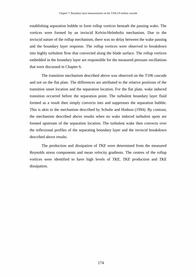
Chapter 7: Boundary layer measurements on the T106 LP turbine cascade
174
establishing separation bubble to form rollup vortices beneath the passing wake. The
vortices were formed by an inviscid Kelvin-Helmholtz mechanism. Due to the
inviscid nature of the rollup mechanism, there was no delay between the wake passing
and the boundary layer response. The rollup vortices were observed to breakdown
into highly turbulent flow that convected along the blade surface. The rollup vortices
embedded in the boundary layer are responsible for the measured pressure oscillations
that were discussed in Chapter 6.
The transition mechanism described above was observed on the T106 cascade
and not on the flat plate. The differences are attributed to the relative positions of the
transition onset location and the separation location. For the flat plate, wake induced
transition occurred before the separation point. The turbulent boundary layer fluid
formed as a result then simply convects into and suppresses the separation bubble.
This is akin to the mechanism described by Schulte and Hodson (1994). By contrast,
the mechanism described above results when no wake induced turbulent spots are
formed upstream of the separation location. The turbulent wake then convects over
the inflexional profiles of the separating boundary layer and the inviscid breakdown
described above results.
The production and dissipation of TKE were determined from the measured
Reynolds stress components and mean velocity gradients. The centres of the rollup
vortices were identified to have high levels of TKE, TKE production and TKE
dissipation.

Chapter 7: Boundary layer measurements on the T106 LP turbine cascade
175
7.8 Figures
Figure 7-1: Measurement grid for boundary layer of T106 LP turbine cascade.
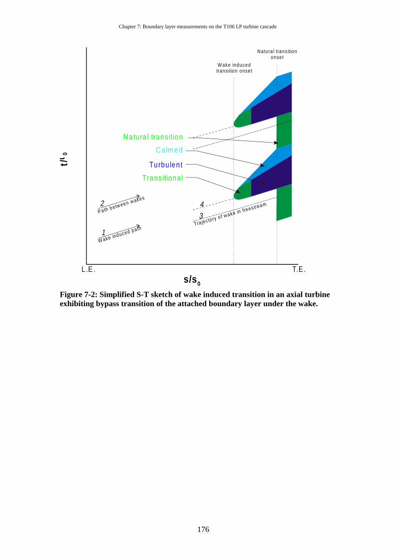
Chapter 7: Boundary layer measurements on the T106 LP turbine cascade
176
Transitiona l
C a lm ed
Turbu len t
34
N atura l trans ition
N atu ra l trans itiononse t
W ake induced trans ition onse t
Tra jec tory o f w ake in frees tream
1
2
W ake induced pa th
P a th be tw een w akes
s/s 0
t
/ τ
0
L .E . T.E .
Figure 7-2: Simplified S-T sketch of wake induced transition in an axial turbine exhibiting bypass transition of the attached boundary layer under the wake.
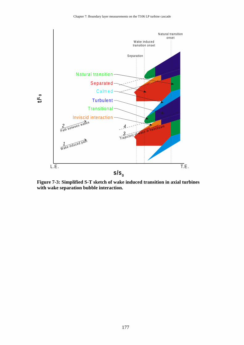
Chapter 7: Boundary layer measurements on the T106 LP turbine cascade
177
s/s 0
t
/ τ
0
L .E . T.E .
Trans itiona l
C a lm ed
Turbu len t
1
2
34
S eparated
N atu ra l trans itiononse t
W ake induced trans ition onse t
W ake induced pa th
P a th be tw een w akes
Tra jec tory o f w ake in frees tream
Inv isc id in teraction
N atura l trans ition
S ep ara tion
Figure 7-3: Simplified S-T sketch of wake induced transition in axial turbines with wake separation bubble interaction.
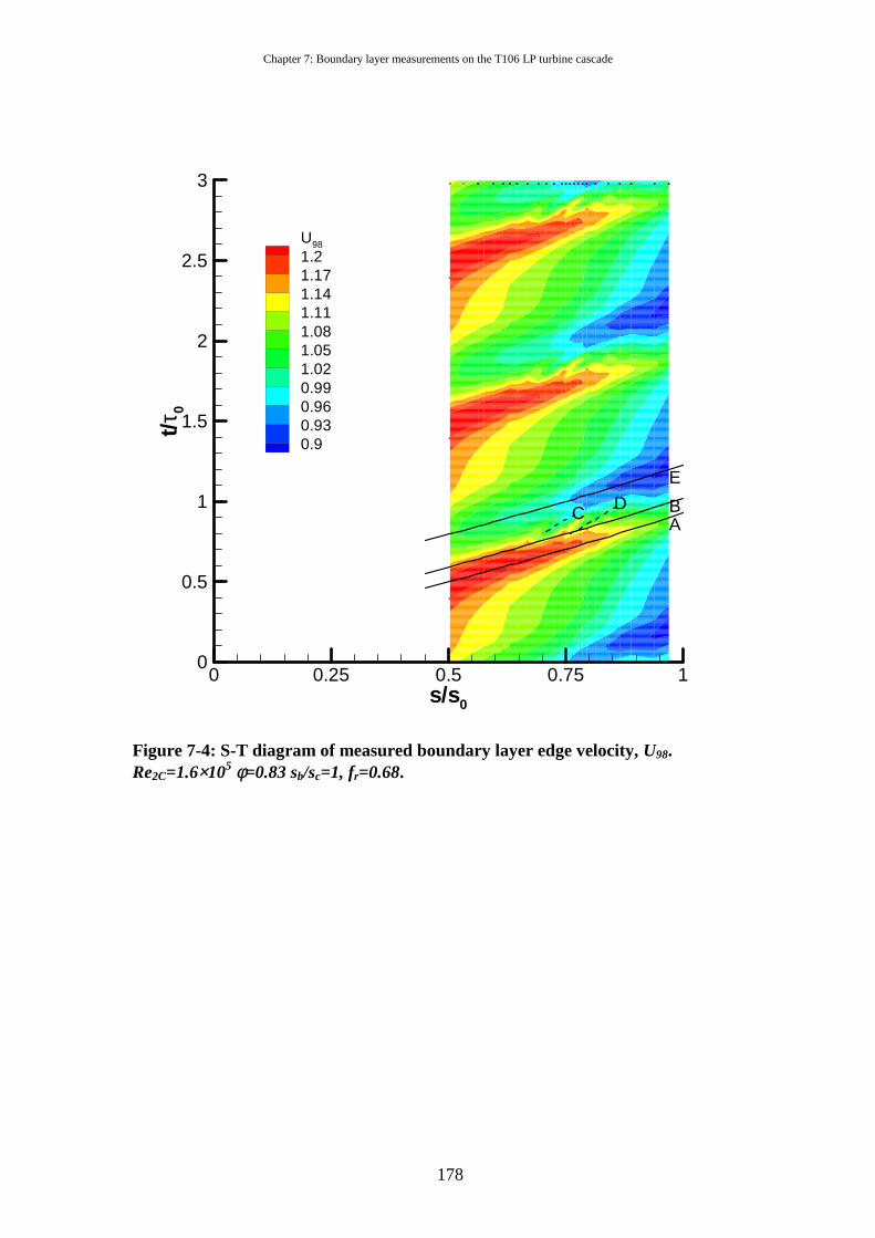
Chapter 7: Boundary layer measurements on the T106 LP turbine cascade
178
0 0.25 0.5 0.75 1s/s0
0
0.5
1
1.5
2
2.5
3t/τ
0
AB
E
DC
U98
1.21.171.141.111.081.051.020.990.960.930.9
Figure 7-4: S-T diagram of measured boundary layer edge velocity, U98. Re2C=1.6×10⁵ φ=0.83 sb/sc=1, fr=0.68.
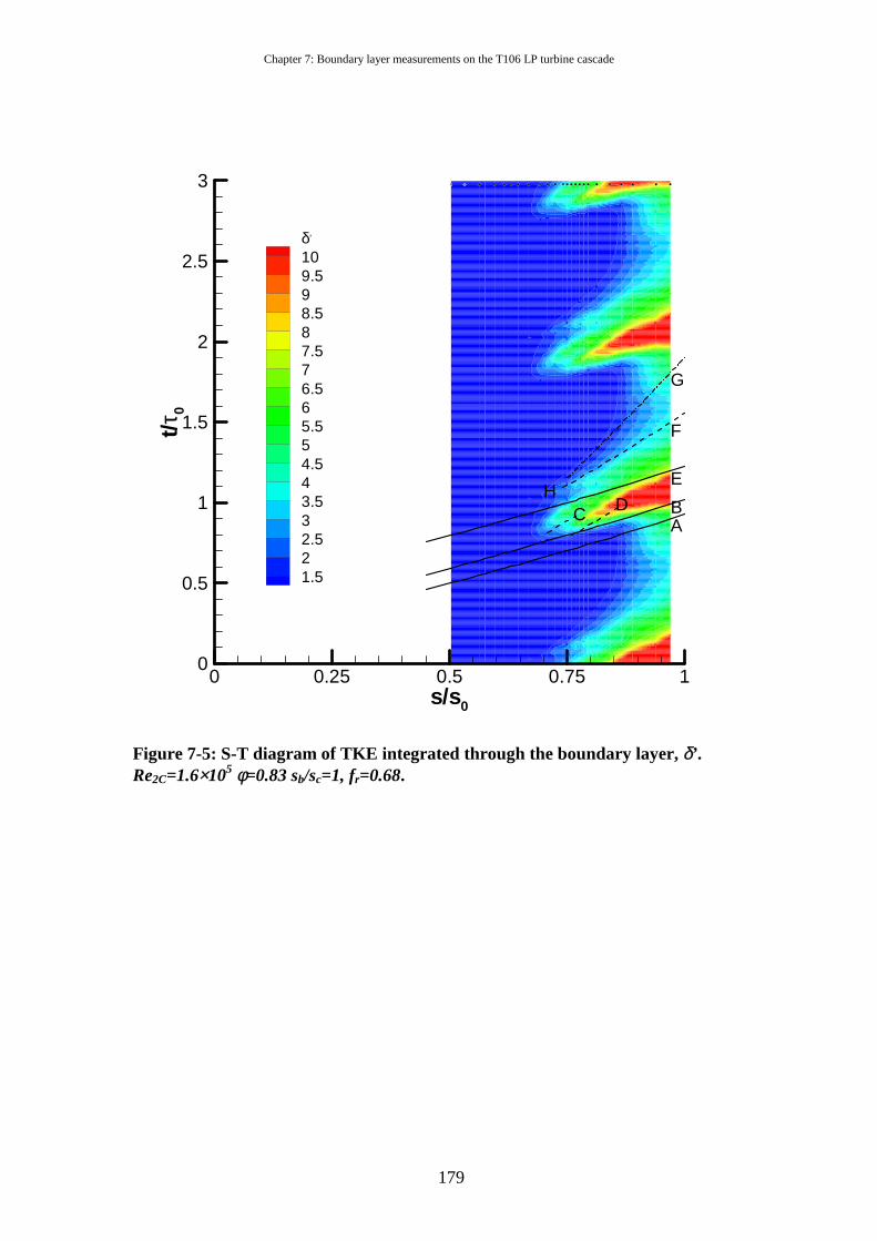
Chapter 7: Boundary layer measurements on the T106 LP turbine cascade
179
0 0.25 0.5 0.75 1s/s0
0
0.5
1
1.5
2
2.5
3t/τ
0
AB
E
D
F
G
HC
δ,
109.598.587.576.565.554.543.532.521.5
Figure 7-5: S-T diagram of TKE integrated through the boundary layer, δ’ . Re2C=1.6×10⁵ φ=0.83 sb/sc=1, fr=0.68.
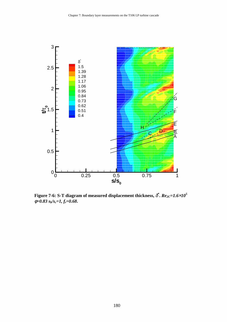
Chapter 7: Boundary layer measurements on the T106 LP turbine cascade
180
0 0.25 0.5 0.75 1s/s0
0
0.5
1
1.5
2
2.5
3t/τ
0
AB
E
D
F
G
CH
δ*
1.51.391.281.171.060.950.840.730.620.510.4
Figure 7-6: S-T diagram of measured displacement thickness, δ*. Re2C=1.6×10⁵ φ=0.83 sb/sc=1, fr=0.68.
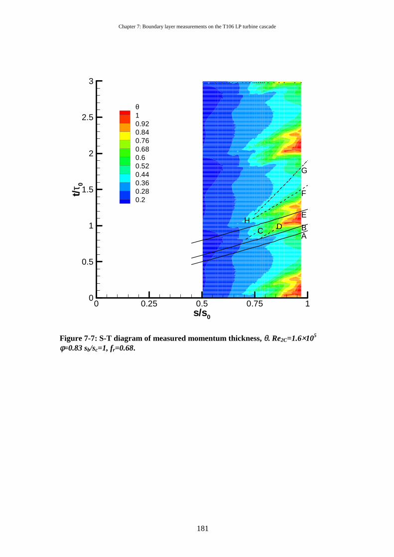
Chapter 7: Boundary layer measurements on the T106 LP turbine cascade
181
0 0.25 0.5 0.75 1s/s0
0
0.5
1
1.5
2
2.5
3t/τ
0
AB
E
D
F
G
CH
θ10.920.840.760.680.60.520.440.360.280.2
Figure 7-7: S-T diagram of measured momentum thickness, θ. Re2C=1.6×10⁵ φ=0.83 sb/sc=1, fr=0.68.
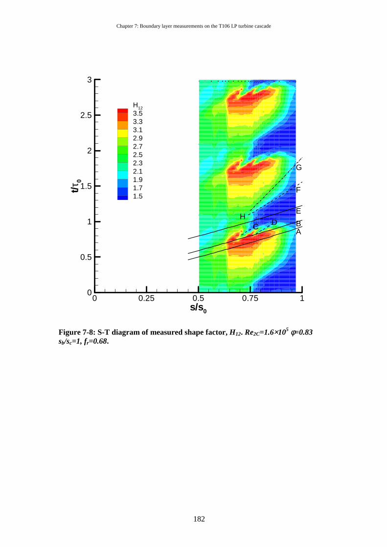
Chapter 7: Boundary layer measurements on the T106 LP turbine cascade
182
0 0.25 0.5 0.75 1s/s0
0
0.5
1
1.5
2
2.5
3t/τ
0
AB
E
D
F
G
CH
H12
3.53.33.12.92.72.52.32.11.91.71.5
Figure 7-8: S-T diagram of measured shape factor, H12. Re2C=1.6×10⁵ φ=0.83 sb/sc=1, fr=0.68.
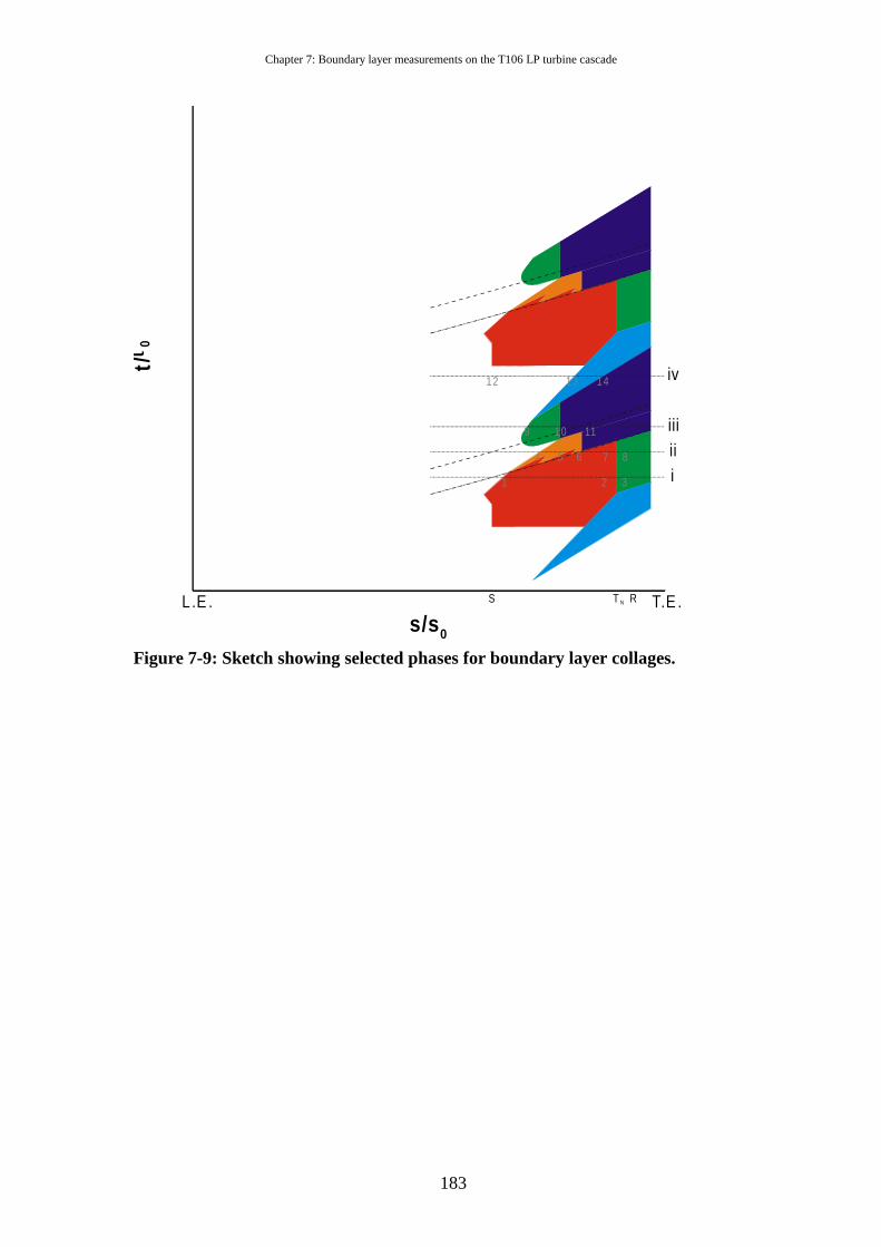
Chapter 7: Boundary layer measurements on the T106 LP turbine cascade
183
s/s 0
t
/ τ
0
L .E . T.E .
iiiiii
iv
S T N R
1 2 3
4 5 6 7 8
9 10 11
12 13 14
Figure 7-9: Sketch showing selected phases for boundary layer collages.
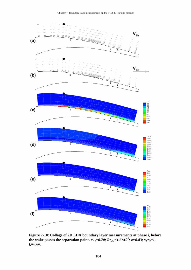
Chapter 7: Boundary layer measurements on the T106 LP turbine cascade
184
1
23
Ω*
-15-30-45-60-75-90-105-120-135-150
(c)
1
23
TKE*
0.050.0450.040.0350.030.0250.020.0150.010.0050.001
(d)
1
23
PTKE*
1.51.351.21.050.90.750.60.450.30.15
(e)
1
23
DTKE*
-0.15-0.3-0.45-0.6-0.75-0.9-1.05-1.2-1.35-1.5
(f)
1
23
V2is
(a)
1
23
V2is
(b)
Figure 7-10: Collage of 2D LDA boundary layer measurements at phase i, before the wake passes the separation point. t/τ0=0.70; Re2C=1.6×10⁵; φ=0.83; sb/sc=1, fr=0.68.
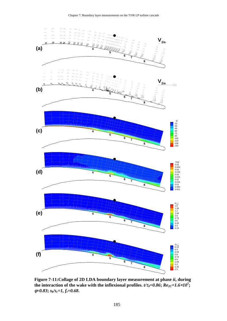
Chapter 7: Boundary layer measurements on the T106 LP turbine cascade
185
56 7
8
4
Ω*
-15-30-45-60-75-90-105-120-135-150
(c)
56 7
8
4
TKE*
0.050.0450.040.0350.030.0250.020.0150.010.0050.001
(d)
56 7
8
4
PTKE*
1.51.351.21.050.90.750.60.450.30.15
(e)
56 7
8
4
DTKE*
-0.15-0.3-0.45-0.6-0.75-0.9-1.05-1.2-1.35-1.5
(f)
65
8
4
7
V2is
(a)
56 7
8
4
V2is
(b)
Figure 7-11:Collage of 2D LDA boundary layer measurement at phase ii , during the interaction of the wake with the inflexional profiles. t/τ0=0.86; Re2C=1.6×10⁵; φ=0.83; sb/sc=1, fr=0.68.
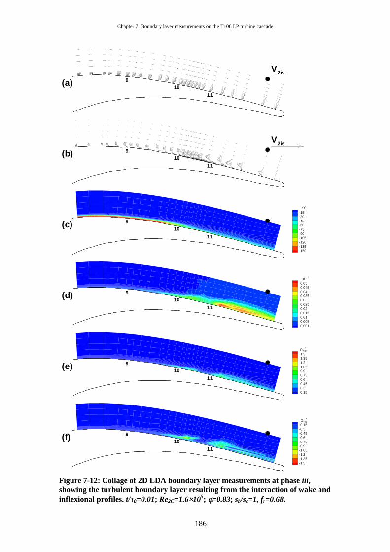
Chapter 7: Boundary layer measurements on the T106 LP turbine cascade
186
910
11
Ω*
-15-30-45-60-75-90-105-120-135-150
(c)
910
11
TKE*
0.050.0450.040.0350.030.0250.020.0150.010.0050.001
(d)
910
11
PTKE*
1.51.351.21.050.90.750.60.450.30.15
(e)
910
11
DTKE*
-0.15-0.3-0.45-0.6-0.75-0.9-1.05-1.2-1.35-1.5
(f)
910
11
V2is
(a)
910
11
V2is
(b)
Figure 7-12: Collage of 2D LDA boundary layer measurements at phase iii , showing the turbulent boundary layer resulting from the interaction of wake and inflexional profiles. t/τ0=0.01; Re2C=1.6×10⁵; φ=0.83; sb/sc=1, fr=0.68.
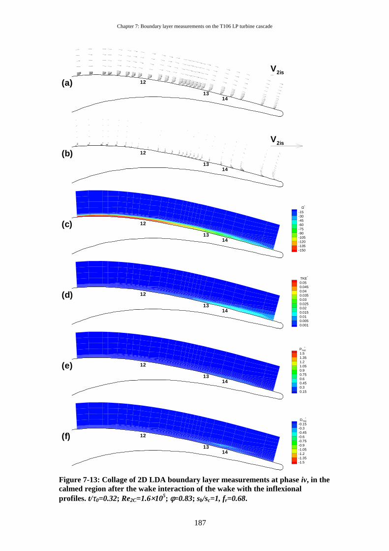
Chapter 7: Boundary layer measurements on the T106 LP turbine cascade
187
12
1314
Ω*
-15-30-45-60-75-90-105-120-135-150
(c)
12
1314
TKE*
0.050.0450.040.0350.030.0250.020.0150.010.0050.001
(d)
12
1314
PTKE*
1.51.351.21.050.90.750.60.450.30.15
(e)
12
1314
DTKE*
-0.15-0.3-0.45-0.6-0.75-0.9-1.05-1.2-1.35-1.5
(f)
12
1314
V2is
(a)
12
1314
V2is
(b)
Figure 7-13: Collage of 2D LDA boundary layer measurements at phase iv, in the calmed region after the wake interaction of the wake with the inflexional profiles. t/τ0=0.32; Re2C=1.6×10⁵; φ=0.83; sb/sc=1, fr=0.68.
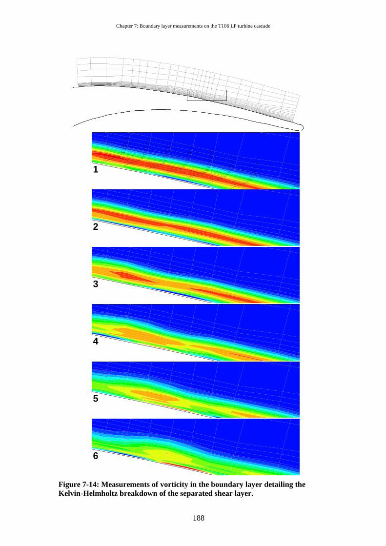
Chapter 7: Boundary layer measurements on the T106 LP turbine cascade
188
1
2
3
4
5
6
Figure 7-14: Measurements of vorticity in the boundary layer detailing the Kelvin-Helmholtz breakdown of the separated shear layer.
189
Chapter 8: Conclusions and recommendations for future work
8.1 Conclusions
8.1.1 Flat Plate The boundary layer of a flat plate subject to a pressure distribution matched to
the T106 LP turbine cascade was measured using 1D LDA and a novel technique to
determine the 2D Reynolds stresses. The unsteady flow conditions were created by a
wake generator using cylindrical bars traversed across the inlet. The bars produced
strong wakes, which resulted in bypass transition upstream of the steady flow
separation point. The wake induced turbulent strip suppressed the separation bubble.
A calmed region followed the wake induced turbulent strip and continued to suppress
separation. As the influence of calming decayed, the boundary layer relaxed to its pre-
transition state and began to separate. During this process, instability waves were
observed in the ensemble average boundary layer measurements. This provides
evidence of deterministic natural transition phenomena arising between wake passing
events. The unsteady flow field provides conditions where the boundary layer is most
susceptible to unstable disturbances for a short time period. Disturbances entering
during this time evolve preferentially and form deterministic structures of wave-
packets in the boundary layer. This phenomenon was observed by Obremski and
Morkovin (1969) for an unsteady flow with a sinusoidal fluctuation of the freestream.
From measurements of the ensemble average mean flow and the full ensemble
average 2D Reynolds stress tensor, it was possible calculate the boundary layer
dissipation on the flat plate. This direct measure of the rate of entropy production in
the boundary layer highlighted the loss reducing mechanisms associated with wake-
induced transition. As expected high levels of dissipation were measured in the wake
induced turbulent strip and low levels in the laminar boundary layer. The calmed
region following the turbulent strip was shown to have laminar levels of dissipation,
as was the separating boundary layer. This confirms that the loss reduction associated
with the interaction of a wake and separation bubble is due to the substitution of the
highly dissipative steady separation bubble flow with calmed and re-establishing
separation flows that are characterised by low dissipation.
Chapter 8: Conclusions and recommendations for future work
190
8.1.2 T106 LP turbine cascade Measurements of the convection of a wake through the T106 LP turbine
cascade were made using 2D LDA and a measurement grid of unprecedented
resolution. These detailed measurements of the 2D Reynolds stresses are intended to
provide a database for the validation of numerical predictions.
Increased levels of TKE were seen to originate about the peak suction location.
This was attributed to the interaction of the elevated turbulent stresses in the wake
passing through a region of strained fluid and thereby acting as a region of TKE
production. Subsequent to this region of high TKE production, the turbulence
associated with the wake was seen to become more isotropic.
A novel adaptation of traditional wavelet transform algorithms allowed an
ensemble averaged wavelet analysis of the randomly sampled LDA data. Results
showed that the Reynolds stress components of the blade-to-blade flow were not
dominated by any particular eddy size.
Unsteady blade surface pressure measurements revealed unexpected high
frequency pressure oscillations with a peak-to-peak magnitude approximately 30% of
the exit dynamic head. The pressure oscillations originated as the wake passed over
the region of the steady flow separation bubble.
Subsequent detailed 2D LDA measurements in the boundary layer revealed
the source of the pressure oscillations to be a series of convected rollup vortices that
formed by an inviscid Kelvin-Helmholtz mechanism when the wake perturbed the
inflexional profiles. These vortices were identified as being localised regions of
elevated production and dissipation of TKE.
Understanding of the mechanism by which the interaction of the wake and
separation bubble results in transition is a crucial element in developing models for
wake-induced transition in highly decelerated boundary layers.
8.2 Recommendations for future work The evidence of instability waves in the ensemble averaged flat plate data
indicates the presence of deterministic natural transition structures. Based on the
ability of the simple quasi-steady en transition model of Obremski and Morkovin
(1969) to predict the evolution of wave packets in a flow with sinusoidal freestream

Chapter 8: Conclusions and recommendations for future work
191
oscillations, it is suggested that such an approach may be applicable in determining
transition in blade surface boundary layers between wake passing events.
No intermittency measurements are presented in this thesis. This is due to the
subjective nature of the threshold selection in highly decelerated flows. It is proposed
that a rigorous intermittency algorithm could be developed based on wavelet spectra.
The instantaneous wavelet spectra could be compared to representative turbulent or
laminar spectra and the intermittency determined on a suitable continuous scale. It
should, however, be borne in mind that the concept of intermittency arose from
transition studies in zero pressure gradient boundary layers where the turbulent and
laminar portions of flow are distinct and may be discriminated in a binary manner. In
separated flows, this simplistic view of turbulence may be misleading and obscure the
true physics of the flow.
The detailed database of wake convection through the T106 LP turbine
cascade is intended for the evaluation of CFD codes. The anisotropy associated with
the wake turbulence suggests that Reynolds stress transport models may be most
suited to correctly reproducing this phenomenon. However, as with all engineering
calculations, the ability of k-ε models and algebraic models to adequately estimate the
convection of turbulent parameters relevant to unsteady by-pass transition prediction
calculations must be determined.
The increased levels of TKE that result from the production of TKE within the
blade passage may prove beneficial in multistage LP turbine environments. The
increasing levels of turbulence may prove more effective in suppressing separations
formed by stronger adverse pressure gradients particularly as the Reynolds number
drops through the machine, which further increases the danger of separation.
The new insights into the transition mechanism resulting from the interaction
of a wake and separating boundary layer should be included in transition models in an
attempt to improve design tools for highly loaded LP turbines. Moreover,
understanding of the transition mechanism may assist in further increasing blade
loading thus further reducing blade counts.
The formation of rollup vortices during the wake-induced transition suggests
that traditional RANS calculations used for turbomachinery design and analysis will
not have sufficient resolution to capture these flow features. In light of this, high-
Chapter 8: Conclusions and recommendations for future work
192
resolution calculations such as DNS or LES may be necessary to suitably predict the
flow. However, the ability of RANS calculations with fine meshes should also be
evaluated as a potential design tool while LES and DNS remain impractical for design
purposes.
The current design process for LP turbine profiles involves simplistic
calculations typically with prescribed intermittency models followed by cascade tests.
Despite the complex transition mechanism involving the rollup of the separated shear
layer, the results of Chapter 7 show that the trajectories of the wake induced turbulent
regions may be adequately described by the correlations of Gostelow et al (1996). It is
proposed that the pressure distribution may be optimised by modelling the onset
location and spot celerities with existing correlations, the starting pressure distribution
could then be adjusted by a numerical optimiser to find the optimal pressure
distribution. Subsequent high-resolution calculations may be used to analyse these
designs and take the place of preliminary cascade testing. As a result, fewer candidate
designs will be tested reducing the development cost and time scale.
Unsteady transition measurements for turbomachines, including those
presented here, have typically been performed at a single spanwise location. As a
result, no information about the spanwise structure of the transition process is
available. This should be investigated using a spanwise array of hot-film gauges and
investigating the cross-correlations between various sensors. The flat plate and
cascade facilities used for the current investigation are only capable of simulating a
two-dimensional flow field. In real machines, the flow field is three-dimensional. In
particular, the wakes are skewed resulting in different wake arrival times along the
span of the blade. The effect of the different arrival times on the transition process and
the interaction between wake and separating boundary layer is unknown. This could
be investigated by orientating the wake generator at an angle to a cascade or flat plate
and performing simultaneous measurements at more than one spanwise location.
The discovery of rollup vortices formed due to the interaction of the wake and
separating boundary layer and their influence on the measured unsteady blade surface
pressures has implications on other areas of aero-engine design. In light of current
demands to reduce air traffic noise, the contribution of the rollup vortices to turbine
noise should be investigated.
193
References Abu-Ghannam, B.J., and Shaw, R., 1980, "Natural transition of boundary layers - the
effects of turbulence, pressure gradient and flow history,” J. Mech. Eng. Sci., Vol. 22, No. 5, pp 213-228.
Addison, J.S. and Hodson, H.P., 1990 a, “Unsteady Transition in an Axial Flow Turbine, Part 1: Measurements on the Turbine Rotor”, ASME Jnl. of Turbomachinery, Vol.112, No2, April 1990, pp206-214.
Addison, J.S. and Hodson, H.P., 1990 b, “Unsteady Transition in an Axial Flow Turbine, Part 2: Cascade measurements and modelling”, ASME Jnl. of Turbomachinery, Vol.112, No2, April 1990, pp215-221.
Addison, J.S., and Hodson, H.P., 1992, "Modelling of Unsteady Transitional Boundary Layers", ASME Jnl. of Turbomachinery, Vol. 114, No. 3, pp 580-589, Jul.
Alam, M. and Sandham, N.D., 2000, “Direct numerical simulation of short laminar separation bubbles with turbulent reattachment”, J. Fluid. Mech., Vol. 410, pp1-28
Banieghbal, M.R., Curtis, E.M., Denton, J.D., Hodson, H.P., Huntsman, I., Schulte, V., Harvey, N.W. and Steele, A.B., 1995, “Wake passing in LP Turbine Blades”, presented at the AGARD conference, Derby, UK, 8.5-12.5.
Bearman, P.W., 1971, “Correction for the effect of ambient temperature drift on hot-wire measurements in incompressible flow”, DISA Information, No. 11, pp. 25-30
Bell, W.A., 1983, “Spectral Analysis Algorithms for the Laser Velocimeter: A Comparative Study”, AIAA Journal, Vol. 21, No. 5
Betchov, R. and Criminale, W.O., “Stability of Parallel Flows”, Academic Press, 1967
Brunner, S., Fottner, L., Schiffer, H-P., 2000, “Comparison of Two Highly Loaded Low Pressure Turbine Cascades under the Influence of Wake-Induced Transition”, ASME 2000GT-268
Chen, K.K. and Thyson, N.A., 1971, "Extension of Emmons” Spot Theory to Flows on Blunt Bodies", AIAA Journal, Vol. 9, No 5, pp 821-825
Cicatelli, G., Hodson, H.P., Dawes, W.N., 1998, BRITE/EURAM CT96-0143, 30 Month Report, May 98- December 98
Cobley, K., Coleman, N., Siden, G., Arndt, N., 1997, “Design of new three stage low pressure turbine for BMW Rolls-Royce BR715 engine”, ASME 97-GT-419
Cox, R.N., 1957, “Wall Neighborhood Measurements in Turbulent Boundary Layers using a Hot-Wire Anemometer”, A.R.C. Report 19191, Feb
Curtis, E.M., Hodson, H.P., Banieghbal, M.R., Denton, J.D. and Howell, R.J., 1996, “Development of blade profiles for low pressure turbine applications”, ASME paper 96-GT-358, International Gas Turbine and Aeroengine Congress and Exposition, Birmingham, UK
D’Ovidio, A., Harkins, J. A., Gostelow, J. P., 2001 a, “Turbulent spots in strong adverse pressure gradients: Part 1 – Spot Behavior”, Proceedings of ASME TURBO EXPO 2001, June, 4-7, 2001, New Orleans, 2001-GT-0406.
D’Ovidio, A., Harkins, J.A., Gostelow, J.P., 2001 b “Turbulent spots in strong adverse pressure gradients part 2- Spot propagation and spreading rates”, Proceedings of ASME Turbo Expo 2001, June 4-7 2001, New Orleans, 2001-GT-0406
References
194
Dovgal, A.V., and Kozlov, V.V., 1990, “Hydrodynamic instability and receptivity of small scale separation regions”, In Laminar-Turbulent Transition, Proc. IUTAM Symp., pp. 523-531, Springer
Dambach, R. and Hodson, H.P., 1999, “ A new Method of Data Reduction for Single-Sensor Pressure Probes”, ASME Paper number 99-GT-304, Presented at the International Gas Turbine and Aeroengine Congress and Exhibition, Indianapolis, Indiana. June 7-10.
Dantec, 1999, “BSA Flow Software Installation and User’s Guide”, Dantec Measurement Technology A/S, Publication Number 9040115712, 4 January 1999.
Denton, J.D., 1993, ”Loss mechanisms in turbomachines”, ASME Journal of Turbomachinery, Vol. 115, No. 4, pp 621-656
Dhawan, S, Narasimha, R, 1958, “Some Properties of Boundary Layer Flow during Transition from Laminar to Turbulent Motion”, J. Fluid Mech. 3, pp. 418-436.
Doorly, D.L. and Oldfield, 1985, “Simulation of the effects of shock wave passing on a turbine rotor blade”, ASME paper No. 85-GT-112
Doorly, D.J., 1988, “Modelling of Unsteady Flow in a Turbine Rotor Passage”, J. Turbomachinery, 110, pp. 27-37.
Dunham, J., 1972, “Predictions of Boundary Layer Transition on Turbomachinery Blades”, AGARD AGARDoGRAPH AG-164, pp55-71
Emmons, H.W., 1951, “The laminar-turbulent transition in a boundary layer- Part 1”, Journal of Aerospace Science, Vol. 18, No7, pp490-498
Farge, M., 1992, “Wavelet transforms and their applications to turbulence”, Annu. Rev. Fluid Mech., Vol. 24, pp395-457
Fujita, H and Kovasznay, LSH, 1969, “Measurements of Reynolds Stress by a Single Rotated Hot Wire Anemometer”, Rev. Sci. Instrum., Vol 39, pp 1351-1355
Gaster, M, 1967, “The Structure and Behaviour of Separation Bubbles” reports and Memo No. 3595, March 1967
Gaster, M., “On transition to turbulence in boundary layers”, in “Transition and Turbulence”, ed. R. E. Meyer, Proceedings of a Symposium, Conducted by the The Mathematics Research Centre, The University of Wisconsin-Maddison, October 13-15, 1980, Academic Press, 1981.
George, W.K., 1975, “Limitations to measuring accuracy inherent in the laser-Doppler signal”, Proc. LDA Symp., Copenhagen
Gibson, W.H., 1970, in “Flow research on blading”, Elsevier Publishing Company Giles, M.B., 1987, “Calculation of Unsteady Wake/Rotor Interactions”, AIAA Paper
87-0006, presented at AIAA 25th Aerospace Sciences Meeting, Reno, Nevada, 1987
Gostelow, J.P., Blunden, A.R., Walker, G.J., 1994, “Effects of free-stream turbulence and adverse pressure gradients on boundary layer transition”, ASME Journal of Turbomachinery, Vol. 116, pp 392-404, July
Gostelow, J.P., Melwani, N. and Walker, G.J., 1996, “Effects of streamwise pressure gradients on turbulent spot development”, ASME Journal of Turbomachinery, Vol. 118, pp. 737-743
Halstead, D.E., Wisler, D.C., Okiishi, T.H., Walker, G.J., Hodson, H.P., Shin, H.-W., 1997 a, “Boundary layer development in axial compressors and turbines: Part 1 of 4 – Composite Picture” Journal of Turbomachinery, vol. 119, pp114-127, January
Halstead, D.E., Wisler, D.C., Okiishi, T.H., Walker, G.J., Hodson, H.P., Shin, H.-W., 1997 b, “Boundary layer development in axial compressors and turbines: Part
References
195
2 of 4 – Compressors” Journal of Turbomachinery, vol. 119, pp114-127, January
Halstead, D.E., Wisler, D.C., Okiishi, T.H., Walker, G.J., Hodson, H.P., Shin, H.-W., 1997 c, “Boundary layer development in axial compressors and turbines: Part 3 of 4 – LP Turbines” Journal of Turbomachinery, vol. 119, pp114-127, January
Halstead, D.E., Wisler, D.C., Okiishi, T.H., Walker, G.J., Hodson, H.P., Shin, H.-W., 1997 d, “Boundary layer development in axial compressors and turbines: Part 4 of 4 – Computations and Analyses” Journal of Turbomachinery, vol. 119, pp114-127, January
Haselbach, F., Schiffer, H-P., Horsman, M., Dressen, S., Harvey, N., Read, S., 2001, "The application of Ultra high Lift Blading in the BR715 LP Turbine”, Proceedings of ASME TURBO EXPO 2001New Orleans, Louisiana, USA, June 4-7, 2001, 2001-GT-0436.
Hatman, A and Wang, T, 1998 a, “Separated-flow Transition. Part 1 – Experimental Methodology and Mode Classification” Presented at ASME Turbo Expo, Stockholm Sweden, 1998
Hatman, A and Wang, T, 1998 b, “Separated-flow Transition. Part 2 – Experimental Results”, Presented at ASME Turbo Expo, Stockholm Sweden, 1998
Hatman, A and Wang, T, 1998 c, Separated-flow Transition. Part 3 – Primary Modes and Vortex Dynamics”, Presented at ASME Turbo Expo, Stockholm Sweden, 1998
Hatman, A and Wang, T, 1998 d, A Prediction Model for Separated Flow Transition”, Presented at ASME Turbo Expo, Stockholm Sweden, 1998
Hodson, H.P., 1984, “Boundary layer and loss measurements on an axial flow turbine”, ASME Jnl. of Engineering for Gas Turbines and Power, Vol. 106, April
Hodson, H.P., 1985, “A Blade-to-Blade Prediction of Wake-Generated Unsteady Flow”, ASME Jnl. of Engineering for Gas Turbines and Power, vol. 107, April 1985
Hodson, H.P., 1989, “Modelling of Unsteady Transition and its Effect on Profile Loss”, in “Unsteady Aerodynamic Phenomena in Turbomachines”, AGARD CP 468
Hodson, H.P., Addison, J.S., and Shepherdson, C.A., 1992, “Models for unsteady wake-induced transition in axial turbomachines”, J. Phys. III France, Vol. 2, No. 4, pp545-574
Hodson, HP and Gostelow, JP, 1999, “Similarities in the development between Triggered Turbulent Spots and Wake-Induced Turbulent Patches”, 37th AIAA Aerospace Sciences Meeting and Exhibit, January 11-14, 199, Reno, NV
Hodson, HP and Schulte. V, 1998, “PUIM users manual”, Whittle Laboratory, Cambridge University
Hodson, HP, 1998, “Bladerow Interactions In Low Pressure Turbines”, in VKI Lecture Series No. 1998-02 Blade Row Interference Effects Axial Turbomachinery Stages, Von Karman Institute, Feb 9-12
Horton, HP, 1969, “A semi-Empirical Theory for the growth and Bursting of Laminar Separation Bubbles”, ARC CP 1073
Hourmouziadis, J, 1989, "Aerodynamic Design of Low Pressure Turbines", AGARD Lecture Series, 167
References
196
Howell, R.J., 1999, “Wake-separation bubble interactions in low Reynolds number turbomachinery”, Ph.D. Thesis, Cambridge University Engineering Department
Howell, R.J., Ramesh, O.N., Hodson, H.P., Harvey, N.W., Schulte, V., 2000, “High Lift and Aft Loaded Profiles for Low Pressure Turbines”, ASME 2000-GT-261.
Howell, R.J., Hodson, H.P., Schulte, V., Schiffer, H-P., Haselbach, F., Harvey, N.W., 2001, “Boundary Layer Development on the BR710 and BR715 LP Turbines – The Implementation of High Lift and Ultra High Lift Concepts”, ASME Paper 2001-GT-0441, Proceedings of the ASME Turbo Expo 2001, June 4-7, New Orleans, LA
Hughes, J.D., Walker, G.J., 2000, “Natural transition phenomena on an axial compressor blade”, Presented at the International Gas Turbine and Aeroengine Congress and Exhibition, Munich, Germany, May 8-11, 2000-GT-264
Jacobs, R.G. and Durbin, P.A., 2001, “Simulations of bypass transition”, J. Fluid Mech., Vol. 428, pp. 185-212
Johnson, M.W., 1993, “A bypass transition model for boundary layers”, 93-GT-90, Presented at the international Gas Turbine and Aeroengine Congress and Exposition, Cincinnati, Ohio, May 24-27
Johnson, M. W., 1998, “Turbulent spot characteristics in boundary layers subjected to streamwise pressure gradient”, 98-GT-124, Presented at the International Gas Turbine and Aeroengine congress and exhibition, Stockholm, Sweden, 2-5 June
Johnson, M.W. and Dris, A., 2000, “The origin of turbulent spots”, ASME Journal of Turbomachinery, Vol. 122, pp88-92, January
Johnson, M.W. and Ercan, A.H., 1996, “A boundary layer transition model”, ASME paper 96-GT-444
Johnson, M.W., Fashifar, A., 1994, “Statistical properties of turbulent bursts in transitional boundary layers”, Int. J. Heat ad Fluid Flow, Vol. 15, No. 4, pp 283-290, August
Klebanoff, P.S., Tidstrom, K.D., Sargent, L.M., 1962, “The Three-Dimensional Nature of Boundary Layer Instability”, J. Fluid Mech., Vol. 12, pp.1-24
Knapp, CF and Roache, PJ, 1968, “A Combined Visual and Hot-Wire Anemometer Investigation of Boundary Layer Transition”, AIAA Journal, Vol 6, Jan 1968, pp 29-36.
Kool, P, 1979, “Determination of Reynolds Stress tensor with a Single Slanted Hot wire in Periodically Unsteady Turbomachinery Flow” ASME Paper 79-GT-130, March.
Kuroumaru, M, Inoue, M, Higki, T, Abd-Elkhalek, FA-E and Ikui, T, 1982, “Measurement of Three Dimensional Flow Field behind an Impeller by means of Periodic Multi-sampling with a Slanted Hot wire”, Bulletin of JSME, Vol. 25, No 209, Nov.
La Graff, J.E., Ashworth, D.A. and Schultz, D.L., 1989, “Measurements and Modelling of the Gas Turbine Blade Transition Process as Disturbed by Wakes”, ASME Jnl. of Turbomachinery, July 1989, vol. 111, pp315-322
LaVision, 2001, ‘DaVis Flowmaster’ v. 6.03, February 2001, LaVision GmbH, Anna-VandenHoeck-Ring 19, 37081 Goettingen, FRG
Li, F. and Widnall, S.E., 1989, “Wave patterns in plane Poiseuille flow created by concentrated disturbances”, J. Fluid Mech., Vol. 208, pp 639-656
References
197
Lin, C.C., 1957, “Motion in the boundary layer with a rapidly oscillating external flow”, Proc. 9th Int. Congress Appl. Mech., Brussels, Vol. 4, pp 155-167
Liu, X. and Rodi, W., 1991, “Experiments on transitional boundary layers with wake-induced unsteadiness”, J. Fluid Mech., Vol. 231, pp. 229-256
Lou, W., Hourmouziadis, J., 2000, “Separation bubbles under steady and periodic-unsteady main flow conditions”, The 45th ASME International Gas Turbine & Aeroengine Technical Congress, Munich Germany May 8-11, paper 2000-GT-0270
Luton, A., Ragab, S., Telionis, D,. 1995, “Interaction of spanwise vortices with a boundary layer”, Phys. Fluids, vol. 7, no. 11, November
Malkiel, E, and Mayle, RE, 1995, “ Transition in a separation bubble”, ASME 95-GT-32.
Mayle, R.E., Schulz, A., 1997, “The path to predicting bypass transition”, ASME Journal of Turbomachinery, vol. 119, pp 405-411, July
Mayle, R.E., 1991, “The role of laminar-turbulent transition in gas turbines engines”, ASME Journal of turbomachinery, Vol. 113 October , 13/509.
Mayle, R.E., 1998, “A Theory for Predicting the Turbulent-Spot Production Rate”, ASME Paper number 98-GT-256
Mayle, R.E., and Dullenkopf, K., 1989, “A Theory for Wake Induced Transition”, ASME paper number 91-GT-57
Merzkirch, W., 1974, “Flow Visualisation”, Academic Press, New York, NY Meyer, R.X. 1958, “The Effects of Wakes on the Transient Pressure and Velocity
Distributions in Turbomachines”, ASME Journal of Basic Engineering, October, pp 1544-1552
Michalike, A., 1991, “On the Stability of Wall Boundary Layers Close to Separation” IUTAM Symposium on Separated Flows and Jets, Springer-Verlag, Berlin, pp. 557-564.
Narasimha, R., 1957, "On the Distribution of Intermittency in the Transition Region of a Boundary Layer", Journal of Aerospace Science, Vol. 24, pp 711-712
Narasimha, R., 1985, “The Laminar Turbulent Transition Zone in the Boundary Layer”, Progress in Aerospace Science, Vol. 22, pp29-80
Narasimha, R., 1998, “Minniwbrook II – 1997 Workshop on boundary layer transition in turbomachines: Post workshop summary”, NASA conference publication 206958, pp. 485-495
Obremski H.J. and Fejer, A.A., 1967, “Transition in oscillating boundary layer flows” Journal of Fluid Mechanics, vol. 29, part 1, July 1967, pp. 93-111.
Obremski, H.J., and Morkovin, M.V., 1969, “Application of quasi-steady stability model to periodic boundary layer flows”, AIAA Journal, Vol. 7, No. 7, pp 1298-1301, July
Obremski, H.J., Morkovin, M.V. and Landhal, M., 1969, “A Portfolio of Stability Characteristics of Incompressible Boundary Layers”, AGARDograph 134, March
Pauley, L.P., Moin, P. and Reynolds, W.C., 1990, “The structure of two-dimensional separation”, J. Fluid Mech. Vol. 220, pp. 397-411
Pfeil, H. and Herbst, R., 1979, “Transition Procedure of Instationary Boundary Layers”, ASME Paper 79-GT-128.
Pfeil, H., and Eifler, J., 1976, “Turbulenzverhaltnisse hinter rotierenden Zylindergittern”, Forschung im Ingeneiurswesen, vol. 42, pp 27-32.
Pfeil, H., Herbst, R. and Schröder, T., 1982, “Investigation of the laminar-turbulent transition of boundary layers disturbed by wakes”, ASME paper 82-GT-124
References
198
Ramesh, O.N. and Hodson, H.P., 1999, “A new intermittency model incorporating the calming effect”, Third European Conference on Turbomachinery: Fluid Dynamics and Thermodynamics, Volume B, 2-5 March 1999, Royal National Hotel, London, UK.
Roberts, W.B., 1980, “Calculation of Laminar Separation Bubbles and their effect of Airfoil Performance”, AIAA Journal, Vol., 18, January
Saathoff, P.J., and Melbourne, W.H., 1997, “Effects of free-stream turbulence on surface pressure fluctuations in a separation bubble”, J. Fluid. Mech., vol. 337, pp1-24
Schlichting, H., 1979, “Boundary-layer Theory”, McGraw-Hill, 7th Edition. Schlichting, H. and Das, A., 1969, “On the influence of turbulence level on the
aerodynamic losses of axial turbomachines”, Proceeding of The Symposium on Flow Research on Blading, Baden, Switzerland
Schubauer, G.B., and Klebanoff, P.S., 1955, “Contributions on the Mechanics of Boundary Layer Transition”, NACA TN 3489 (1955) and NACA Rep. 1289 (1956).
Schubauer, G.B. and Skramstad, H.K., 1947, “Laminar boundary-layer oscillations and transition on a flat plate”, NACA Report No. 909, 1947
Schulte, V., 1995, “Unsteady Separated Boundary Layers in Axial-flow Turbomachinery”, PhD Dissertation, Cambridge University.
Schulte, V. and Hodson, H.P., 1994, “Wake-Separation Bubble Interaction in Low Pressure Turbines”, AIAA/SAE/ASME/ASEE 30th Joint Propulsion Conference and Exhibit, Indianapolis, Indiana
Schulte, V. and Hodson, H.P., 1996, “Unsteady wake-induced boundary layer transition in high lift LP turbines”, ASME Journal of Turbomachinery. vol. 120, pp28-35. January 1998
Schulte, V. and Hodson, H.P., 1999, “Predicting unsteady wake induced transition”, Submitted to ASME 1999.
Smith, L.H., 1966, “Wake Dispersion in Turbomachines”, ASME Journal of Basic Engineering, Vol. 88
Solomon, W.J., Walker, G.J., 1995, “Observations of Wake-Induced Transition on an Axial Compressor Blade”, ASME paper 95-GT-381
Solomon, W.J., Walker, G.J., Gostelow, J.P., 1996, “Transition length prediction for flows with rapidly changing pressure gradients”, ASME Journal of Turbomachinery, Vol. 118, pp 744-751, October
Spiegel, M.R., “Theory and Problems of Vector Analysis and an introduction to Tensor Analysis”, McGraw-Hill, 1974
Stieger, R.D. and Hodson, H.P., 2001, “Reynolds stress measurement with a single component Laser Doppler Anemometer”, submitted to AIAA Journal
Tani, I., 1964, “Low speed Flows involving separation bubbles”, Progress in Aeronautical Science, Pergamon Press.
Tennekes, H., and Lumley, J.L., “A first course in turbulence”, The MIT Press, eleventh printing, 1987
Thwaites, B., 1949, Approximate Calculation of the Laminar Boundary Layer”, The Aeronautical Quarterly, Vol. 1, pp. 245-280.
Torrence, C. and Compo, G.P., 1998, “A Practical guide to wavelet analysis”, Bulletin of the American Meteorological Society, vol. 79, No. 1, January
Truckenbrodt, E., 1952, “ A method of Quadrature for the calculation of laminar and turbulent boundary layers in Plane and Rotational Symmetric Flow”, Ingenieur-Archiv, Vol. 20, translated as NACA TM 1379
References
199
Villermaux, E., 1998, “On the role of viscosity in shear instabilities”, Phys. Fluids, vol. 10, no. 2, February
Volino, R.J., 1998, “Wavelet analysis of transitional flow data under high free-stream turbulence conditions”, 98-GT-289, Presented at the International Gas Turbine & Aeroengine Congress & Exhibition, Stockholm, Sweeden, 2-5 June
Walker, G.J., 1974, “The Unsteady Nature of Boundary Layer transition on an Axial-Flow Compressor Blade”, ASME Paper 74-GT-135
Walker, G.J., 1975, “Observations of Separated Laminar Flow on Axial Compressor Blading”, ASME Paper number 75-GT-63
Walker, G.J., 1987, “Transitional Flow on Axial Turbomachine Blading”, AIAA J. Vol. 27, pp 595-602
Walker, G.J., 1989, “Transitional flow in axial turbomachine blading”, AIAA Journal, vol. 27, no. 5, May
Walker, G.J., 1993, “The role of laminar turbulent transition in gas turbine engines: a discussion”, ASME Jnl. Turbomachinery, Vol. 115, pp 207-217, April
Walker, G.J., and Gostelow, J.P., 1989, “The effect of adverse Pressure Gradients on the Nature and Length of Boundary Layer transition”, ASME Paper number 89-GT-274
Walker, GJ, Subroto, PH and Platzer, MF, 1988, “Transition Modelling Effects on Viscous/Inviscid Interaction Analysis of Low Reynolds Number Airfoil Flows Involving Laminar Separation Bubbles”, ASME Paper number 88-GT-32
Watmuff, J. H., 1999, “Evolution of a wave packet into vortex loops in a laminar separation bubble”, J. Fluid Mech., vol. 397, pp119-169
White, F.M., 1991, “Viscous Fluid Flow”, McGraw-Hill, 2nd Edition. Williams, J. C., 1999, Private communication Wu, X., Jacobs, R.G., Hunt, J.C.R., Durbin, P.A., 1999,”Simulation of boundary layer
transition induced by periodically passing wakes”, J. Fluid Mech., Vol. 398, pp109-153
Zhong, S., Kittichaikarn, C., Hodson, H. P. & Ireland, P. T. 1998, “Visualisation of turbulent spots under the influence of adverse pressure gradients”, In Proc. 8th Intl Conf. on Flow Visualistion, Italy
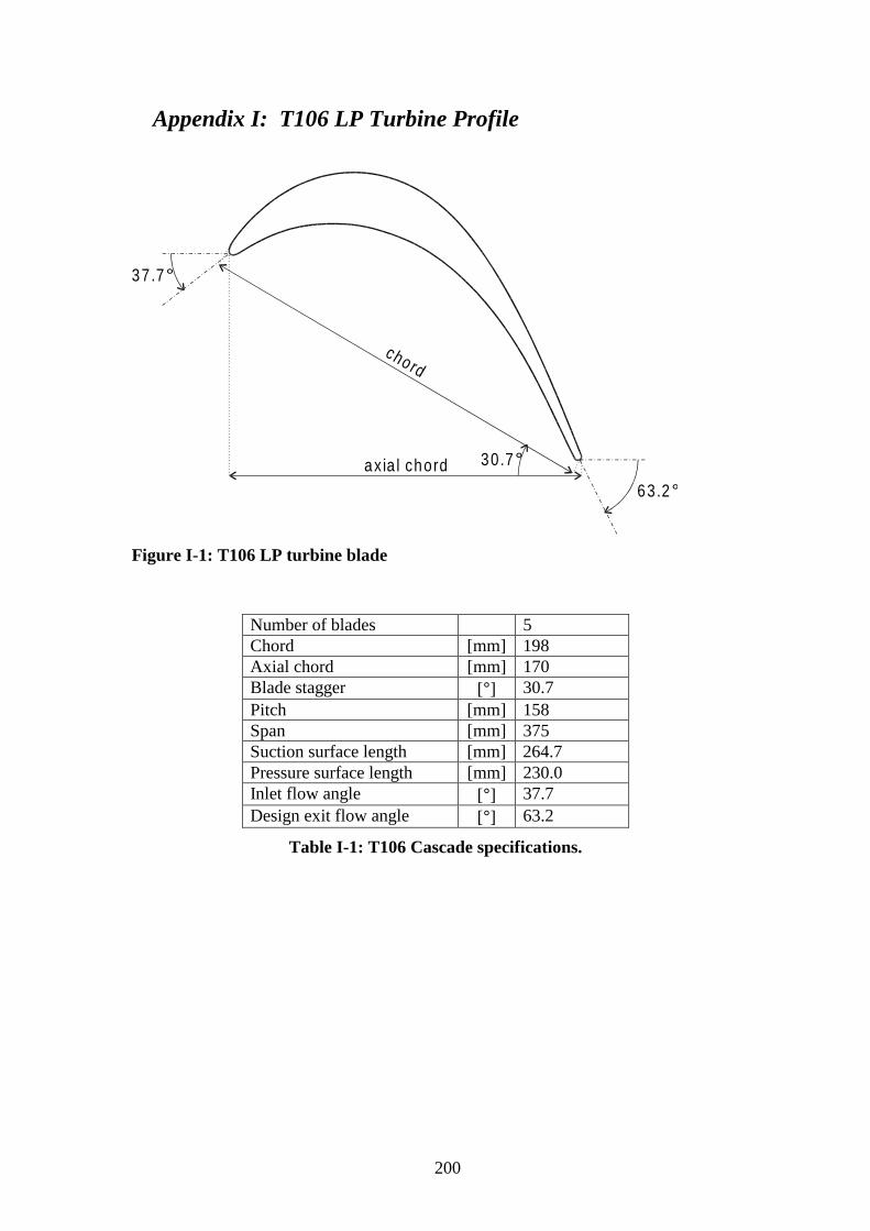
200
Appendix I: T106 LP Turbine Profile
chord
ax ia l chord
37.7°
63.2°
30.7°
Figure I-1: T106 LP turbine blade
Number of blades 5 Chord [mm] 198 Axial chord [mm] 170 Blade stagger [°] 30.7 Pitch [mm] 158 Span [mm] 375 Suction surface length [mm] 264.7 Pressure surface length [mm] 230.0 Inlet flow angle [°] 37.7 Design exit flow angle [°] 63.2
Table I-1: T106 Cascade specifications.
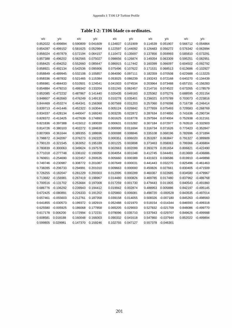
Appendix I: T106 LP Turbine Profile
201
Table I-2: T106 blade co-ordinates.
x/c y/c x/c y/c x/c y/c x/c y/c x/c y/c
0.852022 -0.499894 0.590809 0.041609 0.134837 0.151909 0.114539 0.051907 0.566712 -0.054864
0.854287 -0.499152 0.581625 0.052984 0.122597 0.144092 0.126483 0.056272 0.576342 -0.063994
0.856024 -0.497879 0.572194 0.064157 0.110472 0.135697 0.137856 0.059993 0.585810 -0.073291
0.857388 -0.496202 0.562565 0.075027 0.098656 0.126874 0.149354 0.063309 0.595251 -0.082951
0.858425 -0.494252 0.552660 0.085647 0.086915 0.117442 0.160399 0.066097 0.604502 -0.092792
0.858921 -0.492134 0.542536 0.095906 0.075496 0.107622 0.171531 0.068513 0.613686 -0.102927
0.858849 -0.489945 0.532108 0.105857 0.064090 0.097111 0.182359 0.070508 0.622688 -0.113225
0.858336 -0.487832 0.521465 0.115384 0.053025 0.086239 0.193243 0.072168 0.640270 -0.134439
0.856981 -0.484433 0.510501 0.124541 0.041933 0.074534 0.203964 0.073488 0.657151 -0.156283
0.854884 -0.479210 0.499342 0.133204 0.031245 0.062457 0.214716 0.074522 0.673265 -0.178579
0.852085 -0.472232 0.487867 0.141440 0.020435 0.049183 0.225362 0.075276 0.688595 -0.201154
0.848607 -0.463560 0.476249 0.149133 0.010278 0.035401 0.236021 0.075789 0.703073 -0.223816
0.844469 -0.453274 0.464341 0.156368 0.007569 0.031203 0.257060 0.076098 0.716738 -0.246414
0.839713 -0.441446 0.452322 0.163044 0.005124 0.026842 0.277659 0.075493 0.729583 -0.268769
0.834337 -0.428134 0.440047 0.169240 0.003235 0.022872 0.287634 0.074850 0.741636 -0.290734
0.828372 -0.413425 0.427639 0.174893 0.001625 0.018778 0.297594 0.074004 0.752938 -0.312161
0.821836 -0.397388 0.415012 0.180039 0.000631 0.015282 0.307184 0.072977 0.763519 -0.332903
0.814726 -0.380103 0.402272 0.184630 0.000000 0.011694 0.316734 0.071626 0.773423 -0.352847
0.807069 -0.361644 0.389355 0.188696 0.000088 0.008846 0.335108 0.068196 0.782696 -0.371894
0.798872 -0.342097 0.376273 0.192225 0.000351 0.006020 0.353287 0.063847 0.791327 -0.389909
0.790120 -0.321545 0.363052 0.195189 0.001225 0.003898 0.373463 0.058063 0.799366 -0.406804
0.780839 -0.300063 0.349624 0.197578 0.002663 0.002099 0.393279 0.051654 0.806821 -0.422490
0.771018 -0.277748 0.336102 0.199358 0.004054 0.001048 0.412745 0.044491 0.813669 -0.436886
0.760651 -0.254690 0.322457 0.200535 0.005660 0.000389 0.431923 0.036586 0.819910 -0.449898
0.749746 -0.230987 0.308772 0.201087 0.007649 0.000031 0.441443 0.032270 0.825496 -0.461463
0.738285 -0.206733 0.294991 0.201010 0.009663 0.000000 0.450826 0.027661 0.830405 -0.471509
0.726255 -0.182047 0.281229 0.200303 0.012095 0.000289 0.460367 0.022685 0.834580 -0.479967
0.713682 -0.156981 0.267419 0.198967 0.014480 0.000826 0.469785 0.017480 0.837962 -0.486768
0.700516 -0.131702 0.253684 0.197008 0.017259 0.001730 0.479443 0.011805 0.840543 -0.491860
0.686776 -0.106292 0.239943 0.194412 0.019942 0.002874 0.488953 0.005886 0.842197 -0.495145
0.672425 -0.080891 0.226333 0.191202 0.025860 0.006081 0.498720 -0.000528 0.843535 -0.497014
0.657461 -0.055603 0.212761 0.187358 0.039158 0.014055 0.508326 -0.007180 0.845263 -0.498560
0.641855 -0.030573 0.199372 0.182919 0.052488 0.021970 0.518154 -0.014344 0.846593 -0.499318
0.625580 -0.005925 0.186068 0.177858 0.065205 0.029003 0.527832 -0.021709 0.848086 -0.499770
0.617178 0.006200 0.172994 0.172231 0.078096 0.035710 0.537943 -0.029707 0.849626 -0.499988
0.608581 0.018188 0.160048 0.166003 0.090332 0.041618 0.547860 -0.037944 0.852022 -0.499894
0.599805 0.029981 0.147370 0.159246 0.102755 0.047127 0.557378 -0.046301

202
Appendix II: The use of 1D LDA to measure the full 2D Reynolds Stress Tensor
II.1 Introduction The measurement of the full 2D Reynolds Stress tensor typically requires
multi-axis anemometry systems. By simultaneously measuring multiple velocity
components, it is possible to directly calculate the correlation between the
components of velocity fluctuation and thus to calculate the Reynolds Stress tensor.
However, if the flow is time invariant, or if it is phase locked, it is possible to
combine a series of measurements made at different probe orientations and derive the
time averaged or ensemble averaged Reynolds Stress tensor. This has been
demonstrated by Fujita and Kovasznay (1969), Kuroumaru et al.(1982) and Kool et
al.(1979) who have used the technique in thermal anemometry.
This note details the adaptation of the method of Fujita and Kovasznay (1969)
to Laser Doppler Anemometry (LDA). It is demonstrated that the directional response
of LDA makes it most suitable to this form of measurement. Moreover, the range of
possible measurements obtainable from a 1D system is greatly enhanced with
significant financial savings on equipment purchase. The data collected at multiple
probe angles can also be utilised to enhance the mean flow measurements.
II.2 Derivation The velocity measured by LDA is the component of velocity in the plane of
the intersecting beams and normal to the fringe pattern. If the plane of the beams is
rotated relative to the instantaneous flow velocity vector, U, then only the
instantaneous component of velocity in the plane of the intersecting beams, M, will be
measured according to the cosine relationship
)cos(θUM = (II-1)
where θ is defined in Figure II-2.
The instantaneous velocity component measured by the LDA can also be
written in terms of the instantaneous flow vector components normal and parallel to
the local mean flow (see Figure II-2)
)sin()cos()( θθ vuUM −+= ( II-2)
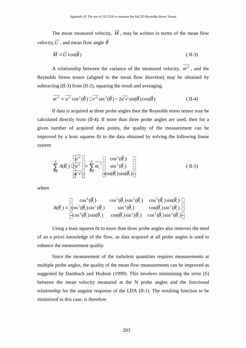
Appendix II: The use of 1D LDA to measure the full 2D Reynolds Stress Tensor
203
The mean measured velocity, M , may be written in terms of the mean flow
velocity,U , and mean flow angle θ
)cos(θUM = ( II-3)
A relationship between the variance of the measured velocity, 2'm , and the
Reynolds Stress tensor (aligned to the mean flow direction) may be obtained by
subtracting (II-3) from (II-2), squaring the result and averaging.
)cos()sin(''2)(sin')(cos'' 22222 θθθθ vuvum −+= ( II-4)
If data is acquired at three probe angles then the Reynolds stress tensor may be
calculated directly from (II-4). If more than three probe angles are used, then for a
given number of acquired data points, the quality of the measurement can be
improved by a least squares fit to the data obtained by solving the following linear
system
∑∑==
=
⋅N
iii
i
i
i
N
ii m
vu
v
u
A1
2
2
22
2
1 )sin()cos(
)(sin
)(cos
''
'
'
)(
θθθθ
θ ( II-5)
where
=
)(sin)(cos)(sin)cos()sin()(cos
)(sin)cos()(sin)(sin)(cos
)sin()(cos)(sin)(cos)(cos
)(2233
3422
3224
iiiiii
iiiii
iiiii
iA
θθθθθθθθθθθθθθθθ
θ
Using a least squares fit to more than three probe angles also removes the need
of an a priori knowledge of the flow, as data acquired at all probe angles is used to
enhance the measurement quality.
Since the measurement of the turbulent quantities requires measurements at
multiple probe angles, the quality of the mean flow measurements can be improved as
suggested by Dambach and Hodson (1999). This involves minimising the error (S)
between the mean velocity measured at the N probe angles and the functional
relationship for the angular response of the LDA (II-1). The resulting function to be
minimised in this case, is therefore
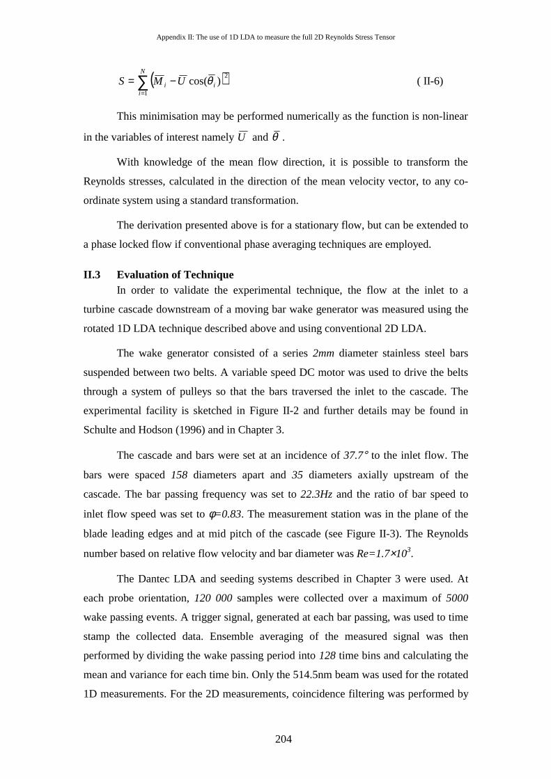
Appendix II: The use of 1D LDA to measure the full 2D Reynolds Stress Tensor
204
( )∑=
−=N
iii UMS
1
2)cos(θ ( II-6)
This minimisation may be performed numerically as the function is non-linear
in the variables of interest namely U and θ .
With knowledge of the mean flow direction, it is possible to transform the
Reynolds stresses, calculated in the direction of the mean velocity vector, to any co-
ordinate system using a standard transformation.
The derivation presented above is for a stationary flow, but can be extended to
a phase locked flow if conventional phase averaging techniques are employed.
II.3 Evaluation of Technique In order to validate the experimental technique, the flow at the inlet to a
turbine cascade downstream of a moving bar wake generator was measured using the
rotated 1D LDA technique described above and using conventional 2D LDA.
The wake generator consisted of a series 2mm diameter stainless steel bars
suspended between two belts. A variable speed DC motor was used to drive the belts
through a system of pulleys so that the bars traversed the inlet to the cascade. The
experimental facility is sketched in Figure II-2 and further details may be found in
Schulte and Hodson (1996) and in Chapter 3.
The cascade and bars were set at an incidence of 37.7° to the inlet flow. The
bars were spaced 158 diameters apart and 35 diameters axially upstream of the
cascade. The bar passing frequency was set to 22.3Hz and the ratio of bar speed to
inlet flow speed was set to φ=0.83. The measurement station was in the plane of the
blade leading edges and at mid pitch of the cascade (see Figure II-3). The Reynolds
number based on relative flow velocity and bar diameter was Re=1.7×10³.
The Dantec LDA and seeding systems described in Chapter 3 were used. At
each probe orientation, 120 000 samples were collected over a maximum of 5000
wake passing events. A trigger signal, generated at each bar passing, was used to time
stamp the collected data. Ensemble averaging of the measured signal was then
performed by dividing the wake passing period into 128 time bins and calculating the
mean and variance for each time bin. Only the 514.5nm beam was used for the rotated
1D measurements. For the 2D measurements, coincidence filtering was performed by
Appendix II: The use of 1D LDA to measure the full 2D Reynolds Stress Tensor
205
software with a coincidence interval of 0.005ms and the Reynolds stress was
calculated for each time bin.
The ensemble averaged results of the 1D rotated LDA and the 2D LDA are
compared in Figure II-4 with only the portion of the period in which the wake passes
shown and the Reynolds stress tensor aligned with the x-y axes of Figure II-3.
Excellent agreement is evident for the ensemble mean data of the two techniques. For
the turbulent statistics, however, the agreement is seen to improve as the number of
angles and thus the total number of samples increases. Estimating the error of the
rotated 1D technique as the average variance from the 2D LDA measurement and
defining the cost of the measurement as the total number of samples used, it is
possible to plot the error of the 1D measurements as a function of cost. Figure II-5
shows the error in ensemble average Reynolds stress, <u’v’>, for a range of numbers
of probe angles, N. Similar results were obtained for the ensemble averaged velocity
variances <u’2> and <v’2>.The highest errors, at all costs, were obtained for case with
N=3. This demonstrates the benefit of using the least squares approach to improve the
quality of the measurements. However, the case of highest N does not give the lowest
error. This indicates that there is an optimum N for a given cost. For a constant cost
experiment, increasing N will reduce the number of samples in each bin from which
statistics are calculated. With inaccurate statistics, the quality of the least squares fit is
compromised.
II.4 Discussion Although the form of (II-4) matches that presented by Fujita and Kovasznay
(1968), it is more precise because the angular response of the LDA is known. The
derivation presented by Fujita and Kovasznay (1969) employed a calibrated
functional fit for the angular response of the hot wire therefore, their derivation
required a Taylor expansion and a small angle approximation. This requires the
fluctuation to be small relative to the mean. However, when the functional response is
known exactly, there is no such limitation and the technique is applicable to flows
with large fluctuations relative to the mean. It should be noted that the least squares
formula presented by Fujita and Kovasznay (1969) assumes that the probe angles are
symmetrically distributed about the flow. The least squares fit presented in (II-5) is a
more general case and places no restriction on the selection of probe angles.
Appendix II: The use of 1D LDA to measure the full 2D Reynolds Stress Tensor
206
This technique retains significant advantages over rotated hot-wires as
discussed by Fujita and Kovasznay (1969). The spatial resolution of the rotated 1D
LDA is far superior to that of a rotated single hot wire and indeed a X-wire. The
measuring volume of the rotated LDA is the same as that for a single orientation and
has a diameter of 0.077mm whereas a rotated single wire sweeps out a circle with
diameter equal to the wire length normal to the flow direction where a typical hot wire
is 1mm long. This means that the rotated hot wire cannot be used to make boundary
layer measurements except in very large-scale experiments, which are impractical for
turbomachinery research. Furthermore, unlike the hot wire technique, there is no
directional ambiguity in the LDA measurements and this remains true for the
technique described here.
II.5 Conclusions A technique for using a single component LDA system to measure the 2D
Reynolds Stress tensor has been presented and found to be in excellent agreement
with the conventional 2D LDA measurements. This technique allows the functionality
of 2D LDA at a capital cost comparable to a single component system.
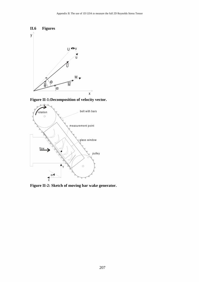
Appendix II: The use of 1D LDA to measure the full 2D Reynolds Stress Tensor
207
II.6 Figures
y
x
U
u
v
M
M
U
αθθ
Figure II-1:Decomposition of velocity vector.
ro ta tion
flow
m easurem ent po int
X
Y
glass w indow
α
pulley
belt w ith bars
Figure II-2: Sketch of moving bar wake generator.
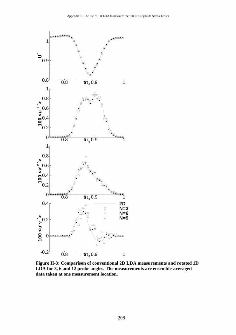
Appendix II: The use of 1D LDA to measure the full 2D Reynolds Stress Tensor
208
t/τ0
100
<u
,v,
* >
0.8 0.9 1-0.2
0
0.2
0.4 2DN=3N=6N=9
t/τ0
10
0<
u,2
* >
0.8 0.9 10
0.2
0.4
0.6
0.8
1
t/τ0
100
<v,
2* >
0.8 0.9 10
0.2
0.4
0.6
0.8
1
t/τ0
U*
0.8 0.9 10.8
0.9
1
Figure II-3: Comparison of conventional 2D LDA measurements and rotated 1D LDA for 3, 6 and 12 probe angles. The measurements are ensemble-averaged data taken at one measurement location.

Appendix II: The use of 1D LDA to measure the full 2D Reynolds Stress Tensor
209
cost
erro
r
103 104 105 10610-5
10-4
10-3
10-2
10-1 N=3N=6N=9N=12
Figure II-4: Error in <u’v’> for rotated 1D LDA for different numbers of probe angles. The 2D LDA measurement is taken as the datum.
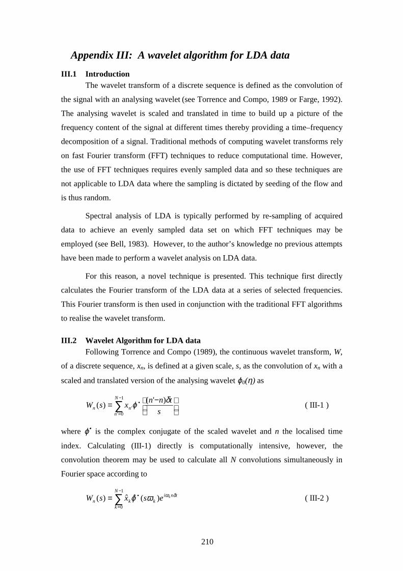
210
Appendix III: A wavelet algorithm for LDA data
III.1 Introduction The wavelet transform of a discrete sequence is defined as the convolution of
the signal with an analysing wavelet (see Torrence and Compo, 1989 or Farge, 1992).
The analysing wavelet is scaled and translated in time to build up a picture of the
frequency content of the signal at different times thereby providing a time–frequency
decomposition of a signal. Traditional methods of computing wavelet transforms rely
on fast Fourier transform (FFT) techniques to reduce computational time. However,
the use of FFT techniques requires evenly sampled data and so these techniques are
not applicable to LDA data where the sampling is dictated by seeding of the flow and
is thus random.
Spectral analysis of LDA is typically performed by re-sampling of acquired
data to achieve an evenly sampled data set on which FFT techniques may be
employed (see Bell, 1983). However, to the author’s knowledge no previous attempts
have been made to perform a wavelet analysis on LDA data.
For this reason, a novel technique is presented. This technique first directly
calculates the Fourier transform of the LDA data at a series of selected frequencies.
This Fourier transform is then used in conjunction with the traditional FFT algorithms
to realise the wavelet transform.
III.2 Wavelet Algorithm for LDA data Following Torrence and Compo (1989), the continuous wavelet transform, W,
of a discrete sequence, xn, is defined at a given scale, s, as the convolution of xn with a
scaled and translated version of the analysing wavelet ϕ0(η) as
∑−
=
•
−=
1
0''
)'()(
N
nnn s
tnnxsW
δϕ ( III-1 )
where ϕ• is the complex conjugate of the scaled wavelet and n the localised time
index. Calculating (III-1) directly is computationally intensive, however, the
convolution theorem may be used to calculate all N convolutions simultaneously in
Fourier space according to
∑−
=
•=1
0
)(ˆˆ)(N
k
tnikkn
kesxsW δωωϕ ( III-2 )
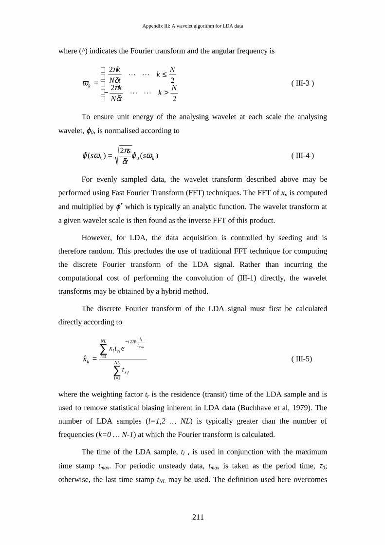
Appendix III: A wavelet algorithm for LDA data
211
where ( ) indicates the Fourier transform and the angular frequency is
>−
≤=
2
22
2
Nk
tN
k
Nk
tN
k
k
δπδ
π
ω ( III-3 )
To ensure unit energy of the analysing wavelet at each scale the analysing
wavelet, ϕ0, is normalised according to
)(ˆ2
)(ˆ 0 kk st
ss ωϕ
δπωϕ = ( III-4 )
For evenly sampled data, the wavelet transform described above may be
performed using Fast Fourier Transform (FFT) techniques. The FFT of xn is computed
and multiplied by ϕ• which is typically an analytic function. The wavelet transform at
a given wavelet scale is then found as the inverse FFT of this product.
However, for LDA, the data acquisition is controlled by seeding and is
therefore random. This precludes the use of traditional FFT technique for computing
the discrete Fourier transform of the LDA signal. Rather than incurring the
computational cost of performing the convolution of (III-1) directly, the wavelet
transforms may be obtained by a hybrid method.
The discrete Fourier transform of the LDA signal must first be calculated
directly according to
∑
∑
=
=
−
=NL
llr
NL
l
t
tki
rll
k
t
etx
x
l
1
1
2max
ˆ
π
( III-5)
where the weighting factor tr is the residence (transit) time of the LDA sample and is
used to remove statistical biasing inherent in LDA data (Buchhave et al, 1979). The
number of LDA samples (l=1,2 … NL) is typically greater than the number of
frequencies (k=0 … N-1) at which the Fourier transform is calculated.
The time of the LDA sample, tl , is used in conjunction with the maximum
time stamp tmax. For periodic unsteady data, tmax is taken as the period time, τ0;
otherwise, the last time stamp tNL may be used. The definition used here overcomes

Appendix III: A wavelet algorithm for LDA data
212
the problem of unevenly sampled data thereby eliminating the need to resample the
LDA data. Consequentially, no spectral noise is added to the wavelet transform. 20
The number of frequencies, N, at which the Fourier transform is calculated dictates
the frequency resolution of the wavelet transform. To facilitate the use of FFT
techniques N is chosen such that N=2n where n is a natural number.
Having calculated the Fourier transform of the LDA data sequence with (III-5)
it is possible to calculate the wavelet transform. The convolution is performed in
Fourier space by multiplying the Fourier transform by the Fourier transform of the
analysing wavelet as in equation (III-2). The inverse Fourier transform necessary to
complete the convolution is then performed by in inverse FFT, which is made
possible by the choice of N.
20 For an evenly sampled sequence xn, the discrete Fourier transform is given by
∑=
−=
N
n
N
nki
nn exN
x1
21ˆ
π. Thus equation (III-5) is identical to this except the factor n/N is replaced by
the factor t/tmax for the unevenly sampled data
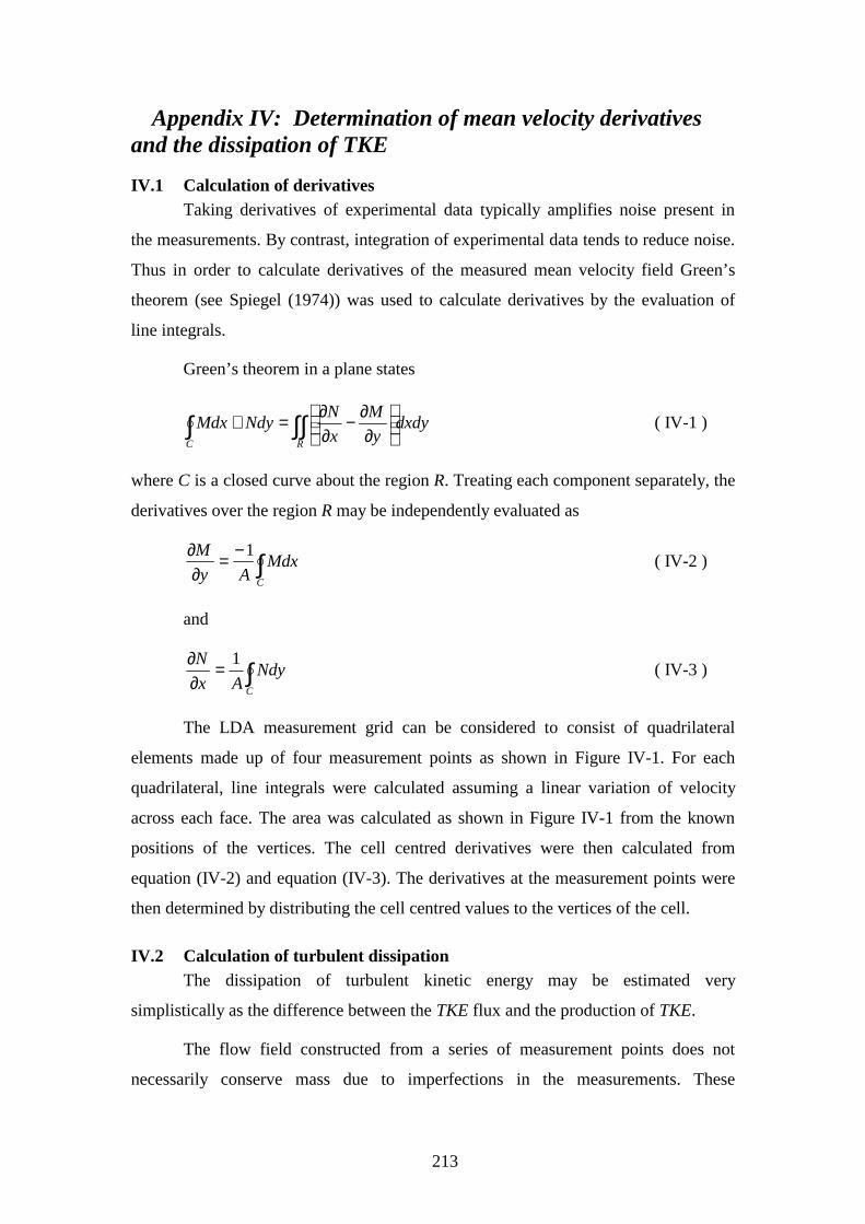
213
Appendix IV: Determination of mean velocity derivatives and the dissipation of TKE
IV.1 Calculation of derivatives Taking derivatives of experimental data typically amplifies noise present in
the measurements. By contrast, integration of experimental data tends to reduce noise.
Thus in order to calculate derivatives of the measured mean velocity field Green’s
theorem (see Spiegel (1974)) was used to calculate derivatives by the evaluation of
line integrals.
Green’s theorem in a plane states
∫∫∫
∂
∂−∂∂=+
RC
dxdyy
M
x
NNdyMdx ( IV-1 )
where C is a closed curve about the region R. Treating each component separately, the
derivatives over the region R may be independently evaluated as
∫−=
∂∂
C
MdxAy
M 1 ( IV-2 )
and
∫=∂∂
C
NdyAx
N 1 ( IV-3 )
The LDA measurement grid can be considered to consist of quadrilateral
elements made up of four measurement points as shown in Figure IV-1. For each
quadrilateral, line integrals were calculated assuming a linear variation of velocity
across each face. The area was calculated as shown in Figure IV-1 from the known
positions of the vertices. The cell centred derivatives were then calculated from
equation (IV-2) and equation (IV-3). The derivatives at the measurement points were
then determined by distributing the cell centred values to the vertices of the cell.
IV.2 Calculation of turbulent dissipation The dissipation of turbulent kinetic energy may be estimated very
simplistically as the difference between the TKE flux and the production of TKE.
The flow field constructed from a series of measurement points does not
necessarily conserve mass due to imperfections in the measurements. These

Appendix IV: Determination of mean velocity derivatives and the dissipation of TKE
214
imperfections may arise from drift in tunnel conditions or measurement noise for
example. The flux of TKE used to estimate dissipation must thus be accounted for.
Consider the 2D flow element, A, shown in Figure IV-2 that comprises four
measurement points. The flow properties on each face of the element are taken as the
average of the values at the vertices and the projection of the element face in the x and
y directions are denoted dSx and dSy respectively as shown in Figure IV-2. The net
mass flux through the faces of the element can be calculated by summation over all
the faces of the element according to
∑ ⋅+⋅=∆∆≈
∂∂
facesyyxx dSVdSV
Attρρρρ 1
( IV-4 )
Similarly, the TKE flux can be obtained,
∑ ⋅⋅⋅+⋅⋅⋅=∆⋅∆≈
∂⋅∂
facesyyfxxf dSVTKEdSVTKE
At
TKE
t
TKE ρρρρ 1)()(
( IV-5 )
however, by applying the chain rule it becomes obvious that there is a contribution to
the measured TKE flux due to changes in mass within the element, which is given by
the last term of
tTKE
t
TKE
t
TKE
∂∂⋅+
∂∂⋅=
∂⋅∂ ρρρ )(
(IV-6 )
By rearranging (IV-6), the TKE flux due only to the production and dissipation
of TKE within the computational cell can be found.
The production of TKE, PTKE, can be found directly from
∂∂+
∂∂−
∂∂+
∂∂=
y
V
x
Uvu
y
Vv
x
UuPTKE '''' 22 ( IV-7 )
using the measured Reynolds stresses values and the velocity derivatives calculated as
described above.
Finally, the dissipation of TKE may be estimated by
TKETKE Pt
TKED −
∂∂≈ ( IV-8 )
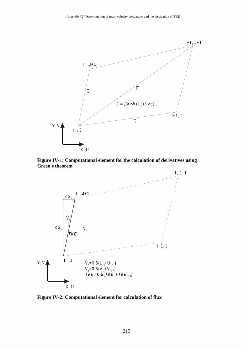
Appendix IV: Determination of mean velocity derivatives and the dissipation of TKE
215
I , J+ 1
I , J
I+ 1 , J
I+ 1 , J+1
X , U
Y, Va
bc
)()( 21
21 cbbaA ×+×=
Figure IV-1: Computational element for the calculation of derivatives using Green's theorem
I , J+ 1
I , J
I+ 1 , J
I+ 1 , J+1
X , U
Y, V
dS y
dS x
V =0 .5 (U +U )x i,j i,j+ 1
V =0 .5 (V +V )y i,j i,j+ 1
T K E T K E TK Ef i,j i,j+1=0 .5 ( + )
V x
V y
T K E f
Figure IV-2: Computational element for calculation of flux