The Effects of Subway Expansion on Traffic Conditions ... · PDF fileEnvironment for Development Discussion Paper Series August 2015 EfD DP 15-22 The Effects of Subway Expansion on

Environment for Development

Discussion Paper Series Augus t 2015 EfD DP 15-22

The Effects of Subway Expansion on Traffic Conditions

Evidence from Beijing

Jun Yang, Shua i Chen, P i ng Q in , and Fangw en Lu

Environment for Development Centers

The Environment for Development (EfD) initiative is an environmental economics program focused on international

research collaboration, policy advice, and academic training. Financial support is provided by the Swedish

International Development Cooperation Agency (Sida). Learn more at www.efdinitiative.org or contact

[email protected].

Central America Research Program in Economics and Environment for Development in Central America Tropical Agricultural Research and Higher Education Center (CATIE) Email: [email protected]

Chile Research Nucleus on Environmental and Natural Resource Economics (NENRE) Universidad de Concepción Email: [email protected]

China Environmental Economics Program in China (EEPC) Peking University Email: [email protected]

Ethiopia Environmental Economics Policy Forum for Ethiopia (EEPFE) Ethiopian Development Research Institute (EDRI/AAU) Email: [email protected]

Kenya Environment for Development Kenya University of Nairobi with Kenya Institute for Public Policy Research and Analysis (KIPPRA) Email: [email protected]

South Africa Environmental Economics Policy Research Unit (EPRU) University of Cape Town Email: [email protected]

Sweden Environmental Economics Unit University of Gothenburg

Email: [email protected]

Tanzania Environment for Development Tanzania University of Dar es Salaam Email: [email protected]

USA (Washington, DC) Resources for the Future (RFF) Email: [email protected]

mailto:[email protected]










Discussion papers are research materials circulated by their authors for purposes of information and discussion. They have

not necessarily undergone formal peer review.

The Effects of Subway Expansion on Traffic Conditions:


Jun Yang, Shuai Chen, Ping Qin, and Fangwen Lu

Abstract

To alleviate traffic congestion, one of the most pressing urban challenges in developing

countries, Beijing’s government has been investing increasingly in subway infrastructure. In this study,

using fine-scale daily traffic records from 2009 to 2013, we perform a regression discontinuity design to

examine the average treatment effects of subway openings on traffic conditions in Beijing from 2009 to

2013. Three findings emerge from our empirical analysis. First, the opening of a new subway line

resulted in a significant decline of daily passenger bus ridership, by 452,400 on average. Second, there

was a significant positive impact on subway passenger ridership, with an average increase of daily

passenger ridership by 246,300 after the opening of each new subway line. Third, we did not find any

significant impact of new subway lines opening on the traffic congestion index, indicating that new

subway openings have not effectively alleviated the traffic congestion in Beijing. Our results are quite

robust to different tests. Our findings imply that subway construction might make it possible that car

users give up vehicles and shift to the subway; however, this “pull” strategy alone is not enough to

reduce congestion.

Key Words: subway construction, regression discontinuity, traffic congestion,

public transportation

JL Codes: L92, R41, R42

Contents

1. Introduction ......................................................................................................................... 1

2. Subway Development in Beijing ........................................................................................ 5

3. Empirical Framework ........................................................................................................ 6

3.1 Regression Discontinuity Design .................................................................................. 6

3.2 Data Description ........................................................................................................... 8

4. Empirical Results .............................................................................................................. 10

5. Robustness Checks ............................................................................................................ 13

5.1 Robustness Check for Various Bandwidths ................................................................ 13

5.2 Robustness Check with Alternative Polynomial Orders ............................................. 13

5.3 Robustness Check for Alternative Sample Set ........................................................... 14

5.4 Robustness Check at Non-discontinuity Points .......................................................... 14

5.5 Robustness Check for Various Time-window Lengths of the Sample Data .............. 15

5.6 Robustness Check with One Particular Subway Line ................................................. 15

6. Conclusion ......................................................................................................................... 15

References .............................................................................................................................. 18

Tables and Figures ................................................................................................................ 21

Environment for Development Yang et al.

1

The Effects of Subway Expansion on Traffic Conditions:


Jun Yang, Shuai Chen, Ping Qin, and Fangwen Lu

1. Introduction

Between 1990 and 2013, total population in Beijing increased from 6.995 million to 21.1

million. The built area in the city proper increased from 397 km2 to 1,268 km,

2 and GDP per

capita grew from 4,653 to 93,213 RMB during the same period. The rapid expansion and income

growth were accompanied by a dramatic increase in vehicle ownership: the number of

automobiles increased from 1.1 to 5.6 million from 2001 to 2014. Once a city of bicycle riders at

the turn of the 21st century, Beijing now is routinely ranked as one of the most polluted and

traffic congested cities in the world. To address traffic congestion, one of the most pressing

urban challenges, the Beijing government has been investing heavily in public transportation

infrastructure in recent years. It is expected that, by 2015, construction of a rail transit network

with 279 stations and a total length of 561 kilometers will be finished in Beijing. Then, the

network density within the 5th Ring Road1 will reach 0.51 km/km

2, and every urban resident will

be able to reach a subway station by walking for only about 1 kilometer.2 Given the large

investment in urban rail transit systems in Beijing, this paper aims to identify the effects of

subway expansion on traffic congestion as well as subway ridership and bus ridership.

The craze for urban rail transit construction in Beijing can be partly explained by the

belief that rail transit construction can reduce vehicle use and thus alleviate congestion.

However, the potential benefits brought about by rail transit may be overestimated. Vickery

Yang, J.: Beijing Transportation Research Center, China (Email: [email protected]); Chen, S.: Guanghua

School of Management and IEPR, Peking University, China (Email: [email protected]); Qin, P.

(corresponding author): Department of Energy Economics, School of Economics, Renmin University of China,

China (Email: [email protected]); Lu, F.: School of Economics, Renmin University of China, China (Email:

[email protected]). Seniority of authorship is shared equally. All correspondence should be addressed to Ping

Qin. Financial support from the National Science Foundation of China (71403279) and the Swedish International

Development Cooperation Agency (Sida), through the Environment for Development (EfD) initiative, is gratefully

acknowledged.

1 Beijing has a system of ring roads; the ring road nearest to the city center is the 2nd ring road, and the 6th ring road

is the farthest away.

2 Source: Action Plan for Green Transportation Construction in Beijing based on the Concepts of Humanism,

Science and Environmental Protection (2009-2015).






2

indicated as early as 1969 that subway construction can reduce the use of vehicles by being an

alternative means of commuting, but, at the same time, the improvement of traffic conditions

may induce more commuting by vehicles. So, it is difficult to determine the exact impact of

subway expansion on the use of vehicles. As a result, the ultimate impact of subway construction

and expansion on urban congestion and air pollution is undetermined.

Although Beijing has been constantly building new lines in recent years, traffic

congestion does not show significant improvement. The average driving speed on the road

network of Beijing's downtown area during the morning peak was 26.4 km/h in 2011 and 26

km/h in 2012. This speed increased to 27.4 km/h in 2013, only a slight increase of 1 km/h

compared with 2011.3 This seems to suggest that the benefits from subway expansion in Beijing

might not be as significant as expected by the government and public; however, mostly due to a

lack of Chinese data, there is little empirical evidence of its magnitude. In this study, we perform

regression discontinuity (RD) analysis to explore the relationship between subway opening and

bus ridership, subway ridership, and, more importantly, the traffic congestion index in the

Beijing central city area, taking advantage of a unique data set provided by the Beijing

Transportation Research Center. With this econometric approach and unique data set, we believe

we are able to alleviate several identification issues present in most previous literature. First,

based on cross-sectional data, several studies investigate the effects of subway lines on travel

behavior as well as on the associated congestion or air pollution by comparing commuting

methods between a treatment group and a control group (Kain and Liu 1994; Petitte 2001).

However, this method could be easily affected by self-selection bias because the residents who

choose to live along the subway lines are more likely to prefer travel by subway. Moreover, the

residents living near and further away from subway stations may differ in several dimensions

such as income, age, educational background and vehicle ownership, which make these two

groups unsuitable for comparison (Gordon and Willson 1984; West 2004; Feng et al. 2013). The

second potential identification issue is simultaneity. The government may selectively choose to

build subways in areas where the demand for automobile travel is relatively higher or the

congestion situation is much worse, and hence congestion is likely to be elevated anyway. Such

an endogeneity problem could pose a significant challenge to the credible estimates that are

required to solve the identification issue. Third, to overcome the self-selection bias that is

persistent in cross-sectional data, a difference-in-difference method can be used to explore the

3 Data source: Beijing Transportation Research Center, 2013.


3

impact of subway construction on travel behavior (Xie 2012). Unfortunately, such studies are

still not free from self-selection bias. The core of the DID method is to compare the differences

between the treatment group and the control group before and after the policy shock. The

rationale for such an approach is that the time trend of the two groups should be consistent.

When there is no treatment group (the subway is either operating or not), there is no hypothetical

treatment group that could accurately measure the true causality effects related to the policy (or

shock). Therefore, these estimates are bound to raise arguments and doubts.

In light of these concerns, we use the RD method to estimate the marginal treatment

effects of the subway opening on public transportation ridership and traffic congestion. This

analysis was performed based on the following assumption: the opening date of the new subway

line was taken as the threshold; if there was no other transportation policy introduced before or

after this opening date (within the sample range) – or if there was, but the observables or

unobservables could affect the dependent variables smoothly in the neighborhood of the subway

opening date – then, the occurrence of the discontinuity point in the regression could be

attributed to the opening of the new subway line. The central assumption of this approach is that

the dependent variables should change smoothly over time-series observations around the

opening day threshold. In order to isolate the change in dependent variables solely due to the

opening of new subway lines, polynomial time trends are usually used to control for non-linear

effects arising from other confounding factors (see, for example, Gibbon and Machin 2005 and

Davis 2008).

We studied the average treatment effects of the five new subway lines that operated

during 2009-2013 in Beijing. Three findings emerge from our empirical analysis. First, a

significant and negative impact was found on bus passenger ridership. On average, the opening

of each new subway line resulted in a decline of daily bus ridership by 452,400. Second, there

was a significant positive impact on subway passenger ridership, with an average increase of

daily ridership by 246,300 after the opening of each new subway line. Third, we did not find

significant impact of new subway lines on the traffic congestion index, including the all-day

average index, morning peak index and evening peak index. We also conducted a series of

robustness tests, i.e., a number of alternative specifications, including different samples and

randomly chosen thresholds. The results are quite robust to these tests.

We speculate on two possible explanations for why subway expansion did not effectively

alleviate the traffic congestion. First, it might be that a new subway opening diverts riders mostly

from buses or even generates new riders from those who walked or rode bicycles. In such cases,

subway expansion is not a substitute for vehicles. Second, even if subway expansion has a


4

substitution effect on vehicles, the improvement of traffic conditions might induce more

commuting by vehicles. Consequently, the roads are still as congested as before.4 Though

subway construction makes it possible for car users to give up the car and transfer to the subway

system, the evidence of our study demonstrates this “pull” strategy alone is not enough.

Our study offers the following contributions. First, it facilitates a better understanding of

the contradictions and challenges encountered during the simultaneous process of motorization

and urbanization taking place in large and medium-sized cities in China. In the early stage of

China's motorization, the government failed to take actions to inhibit the explosive growth of

vehicles, which led to the phenomenon of a larger vehicle population in the more densely

populated areas. This seriously violates good practices of motorization development of large

cities in other parts of the world. During a motorization process that is not planned or regulated,

vehicles are intensively used within distances that can be covered by bus or walking. This

directly results in unnecessary traffic congestion and air pollution (Li 2014; Yang et al. 2014; Li

et al. 2014; Sun et al. 2014; Xie 2012).

Second, our research can also contribute to the design of effective transportation policies

to control traffic congestion in other Chinese cities. Currently, some second-tier and third-tier

cities and even a few counties in China are also constructing their first subway lines. At present,

38 cities have been approved by the central government to construct at least one subway line

before 2020 (Dong and Wu 2013). It is estimated that, by 2020, the mileage of China's rail transit

will reach 6000 kilometers, accounting for over 40% of the total mileage of rail transit in the

world. The total investments in rail transit will approach 4,000 billion RMB.5 Therefore, whether

as an experience or a lesson, the efforts made by Beijing to reduce traffic congestion through a

shift to green transportation, with subway expansion as the focus, can be referred to by those

cities.

Third, our work adds to the rich literature that identifies the effects of public transport on

traffic congestion alleviation. In the existing literature, no consensus is reached on the alleviating

4 Because data on vehicle flow is unavailable, these two possibilities cannot be further analyzed. Analyzing data

from a household survey of Beijing residents' travel in 2007-2009, Xie (2012) found that subway use increased by

98.3% and vehicle use decreased by 19.8% after subway expansion. This result supports the substitution effect of

the subway on vehicles. Based on this analysis, the second explanation is more likely to be true.

5 Data source: A Bird's-Eye View on Metros, Metrobits: http://mic-ro.com/metro/metrostats.html.

http://mic-ro.com/metro/metrostats.html


5

effect of public transport infrastructure, and most work is done in developed countries. For

example, Anderson (2014)6 used a regression discontinuity design to study a sudden strike in

2003 by Los Angeles transit workers. He found that the average highway delay increases 47%

when transit service ceases. This in turn demonstrates that the net benefits of transit systems

appear to be much larger than previously believed. Nelson et al. (2007) estimated the travel

benefits of the local transit system to transit users and the congestion-reduction benefits to

motorists in the Washington, D.C., metropolitan area, using a simulation model in which travel

decisions are modeled as a nested logit tree. They calculated that the Washington transit system

reduces total congestion by 184,000 person-hours per day, or 2.0 person-minutes per peak transit

passenger mile carried. On the other hand, using metropolitan-area data, Winston and Langer

(2006) estimated that, although rail lines reduce congestion, bus lines increase congestion; the

net effect of transit systems is thus to increase congestion. Duranton and Turner (2011)

investigated the relationship between interstate highways and highway vehicle kilometers

traveled (VKT) in US cities and estimated a positive relationship between bus fleet size and

vehicle miles traveled (VMT). They concluded that increased provision of roads or public transit

is unlikely to relieve congestion.

The remainder of the paper is organized as follows. Section 2 provides an overview of

Beijing's subway development. Section 3 presents the empirical framework and data. Section 4

discusses the empirical results. Section 5 provides robustness tests and Section 6 concludes.

2. Subway Development in Beijing

Before 2000, there were only two subway lines (Line 1 and Line 2) in Beijing. Line 1,

completed in 1969, is the first subway line in China, by which Beijing's downtown area,

Chaoyang District and western suburbs were connected. In 2004, Line 1 was extended at the

eastern section by the newly built Batong Line, which connects with the Tongzhou District in the

eastern suburbs. Line 2 was first operated back in 1987; it is a loop line in Beijing. Built along

the old urban district of Beijing, Line 2 overlaps with the Second Ring Road in the eastern,

northern and western sections. In the following 15 years, no new subway lines were built in

6 The magnitude of the effect of ceasing operation of a subway or line and that of opening a subway or line may be

asymmetric. One reason is that commuters need time to adjust to the changes. So, the magnitude of the effects of

ceasing subway operation is likely to be more similar to the long run effects of opening a subway than to the effects

we study at the discontinuity.


6

Beijing. It was not until 2002 that another subway line, Line 13, began operation. This line starts

from Xizhimen Station in the west and ends in Dongzhimen Station in the east, with a total

distance of 40.5 kilometers and 16 stations.

As part of the preparations for the 2008 Olympic Games, the Beijing government

invested heavily in the construction of subway infrastructure. At least one subway line has been

added every year since 2007. The development of the Beijing subway after 2007 is

unprecedented around the world. Beijing's investments in transportation infrastructure from 2007

to 2013 exceeded RMB 300 billion. Twelve subway lines and one airport express were

constructed, with an increase of operational mileage by 351 kilometers. Moreover, another 12

subway lines are currently under construction and will be opened in late 2015. By then, the total

operational mileage of Beijing subways will approach 561 kilometers.

In this study, nine subway lines opened in 2009-2013 are investigated. These are Line 4,

Line 15 (Phase 1), the Changping Line (Phase 1), the Daxing Line, the Fangshan Line, the

Yizhuang Line, Line 9, Line 6 and Line 14; see Fig. 1. Line 4 was put into operation on

September 28, 2009, facilitating north-south transport in western Beijing. The total length of

Line 4 is 28.2 kilometers, with a total of 24 stations (see Table 1). Line 15 (Phase 1), the

Changping Line (Phase 1), the Daxing Line, the Fangshan Line, and the Yizhuang Line opened

at the same time; they link the new towns in the suburbs, with a total distance of 122.4

kilometers and 54 stations. Line 9, opened on December 31, 2011, is the longitudinal trunk in

western Beijing. It intersects with Line 4, Line 6, Line 1 and the Fangshan Line, with a total

distance of 16.5 kilometers and 13 stations. Line 6 (Phase 1), opened in December 2012, is a

transmeridional trunk running through the central city. Its total distance is 30.4 kilometers with

20 stations. The western section of Line 14 was put into operation in May 2013, with a total

distance of 12.4 kilometers and 7 stations. The completed Line 14 will be an L-shaped line that

connects the northeast and the southwest. By May 2013, the total mileage of the five lines was

210 kilometers, accounting for 45% of the total operational mileage (465 kilometers) of the

Beijing subway. The distribution of the five subway lines in relation to the ring roads in Beijing

is shown in Fig. 1.

3. Empirical Framework

3.1 Regression Discontinuity Design

This study estimates the average marginal treatment effect of the opening of new subway

lines on public transportation, with a focus on the impact of new lines opening on traffic


7

congestion in the Beijing central city area. A sharp regression discontinuity design is used for

this estimation strategy. According to Angrist and Pischke (2008), when there is only one

discontinuity point of intervention, the local average treatment effect (LATE) β1 can be estimated

using the equations below:

0 1 2 ( ) t t t t tBPV Treat f X Z

(1)

0 1 2 ( )t t t t tSPV Treat f X Z

(2)

0 1 2 ( ) t t t t tTCI Treat f X Z u (3)

where BPVt and SPVt are the bus and subway passenger ridership, respectively, on the t-th day.

TCIt represents the congestion index on the t-th day (including the congestion index during the

morning and evening peak, as well as the average daily congestion index). Treatt is the dummy

variable indicating whether or not the new subway line is open on the t-th day; 0 indicates not

open while 1 indicates already open. Xt is the number of days from the date of the new subway

line opening to the t-th day, characterizing the time between the sample point and the

discontinuity point. Here we call Xt the predictor. Before the opening of the new subway line, Xt

takes a negative value; after the opening, Xt takes a positive value; on the day of opening, Xt is

denoted as zero. F(Xt) is the k-th order polynomial function, used to flexibly control for time-

series variation in the passenger ridership or congestion that would have occurred in the absence

of the opening of the subway lines. Zt represents other control variables, including the dummies

such as extreme weather, weekday and holiday.

Some estimation details need to be discussed here. Firstly, to use RD design to evaluate

the causal effect of new subway lines opening, one central assumption is that the observables or

unobservables affect the dependent variables smoothly in the neighborhood of the subway

opening date. Therefore, in the regression equation, we use a higher-order term of Xt to control

for the non-linear effect of the unobservable factors on outcome variables. Secondly, an

important issue in practice is the selection of the smoothing parameter, the bandwidth h. When

we use a nonparametric estimation approach, the variation range of the forcing variable Xt is

divided into K bins according to a certain bandwidth h. Subsequently, the outcome variable in

each bin is simulated piecewise (Imbens and Lemieux 2008). Generally, the range of the bin

should not be too narrow or too wide. If bins are too narrow, the estimates will be highly

imprecise. In practical terms, the problem is that, in finite samples, the bandwidths have to be


8

large enough to encompass enough observations to get a reasonable amount of precision in the

estimated values of treatment effects. If they are too wide, the estimates may be biased because

they fail to account for the slope in the regression line, which is negligible for very narrow bins

(Lee and Lemieux 2010). The estimation method in our study is local polynomial regression. In

practice, a cross-validation procedure is recommended to determine the optimal bandwidth

(Imbens and Lemieux 2008). Third, in order to ensure the effectiveness and robustness of the

estimation, a series of robustness tests was conducted, including different higher-order terms,

bandwidths, samples and length of the sample. Fourth, due to the lack of detailed data

concerning the use of vehicles and taxis, the degree of the substitution effect on different

commuting methods induced by opening of the new subway line cannot be analyzed precisely.

Here, by analyzing the impact on traffic congestion and on bus and subway passenger ridership,

we limit our further exploration to the possibility of replacing car trips with commuting by

subway.

3.2 Data Description

Our data include daily passenger trips by bus and subway as well as the traffic congestion

index for the central city in Beijing from August 2009 to July 2013. The date when the subway

line of interest was opened during this period was taken as the discontinuity point. With each

discontinuity point as the origin, the relevant data 60 days before and after the opening of each

subway line were observed, and therefore a total of 605 observed values were obtained for the

five batches of subway lines opened during this period. We decided to use 60 days before and

after the opening of the subway as the sample period to ensure no overlap between the sample

periods of each subway line. For example, the sample periods of Line 6 and Line 14 were very

close, but there was no overlap. The last day of the sample period after the opening of Line 6 was

February 28, 2013, while the first day of the sample period of Line 13 was March 6, 2013.

Detailed information concerning the subway samples is shown in Table 1.

The daily passenger ridership of bus and subway data was from Beijing Daily Transport

Operation Monitoring, released by the Transport Operation Control Center of Beijing. The daily

traffic congestion index (TCI), as the measure of motorized traffic speed in Beijing’s central city,

is provided by the Beijing Transportation Research Center.


9

TCI7 is an aggregated index of road congestion that is calculated using real-time speed

and location of 40,000 floating cars within the 5th Ring Road, weighted according to traffic

volumes of each road link. The index describes the relationship between travel time according to

real-time speeds on the road and travel time in obedience to the road's speed limit (Zhong 2015).

TCI is scaled between 0 and 10, with 0 meaning no congestion at all and 10 referring to complete

congestion. The available TCI data8 covers morning and evening peak traffic and daily average

traffic between August 2009 and July 2013.

In addition, we are concerned with extreme weather that may affect the commuting

choices. Our analysis focuses on five types of extreme weather: heat wave, cold spell, rainstorm,

gale and snow. The definitions of these extreme weather conditions were based on meteorology.9

High temperature and heat wave usually refer to weather with air temperature higher than 35°C

for several consecutive days. A cold spell is defined as a rapid fall in temperature by over 8°C

within 24 hours (or a fall by over 10°C within 48 hours) when cold air passes through a region

and the lowest temperature declines to below 4°C. Rainstorm refers to heavy rain with

precipitation of 50 mm or above within 24 hours. Meteorologically, gale refers to a wind of

Grade 8 strength, with wind speed of 17.2-20.7 m/s. Snow is defined as snowfall of 1.0-3.0 mm

within 12 hours, snowfall of 2.5-5.0 mm in 24 hours, or snow depth reaching 3cm.

Information about official holidays and off-duty shifts was obtained from the notice of

yearly holiday arrangements released by the General Office of the State Council and arranged by

the authors. The statistical information about the variables discussed above is shown in Table 2.

7 The team that designed and implemented TCI includes the Beijing Transportation Research Center, Beijing

Jiaotong University, and ERTICO, which stands for ITS Europe, the network of Intelligent Transport Systems and

Services stakeholders in Europe. Since 2010, the TCI has been formally incorporated into national standards

and has become a set of normative guidance documents.

8 For example, Sun et al. (2014) used the traffic congestion index to quantify driving restrictions’ effects on traffic.

They found a significant and positive impact on traffic congestion with the driving restriction program. Using TCI

data and leveraging the variation in the last digit of vehicles’ license plate numbers, Zhong (2015) found that traffic

congestion is 20% higher on days when the vehicles with license plate numbers ending in 4 and 9 are banned.

9 http://baike.baidu.com/.

http://baike.baidu.com/


10

4. Empirical Results

Based on equation (1), we used the RD method to estimate the marginal effect on bus

ridership of the new subway line opening. The estimation results are reported in Table 3. In

column 1, we include only the dummy variable indicating the opening of the new subway line,

the first order term of the forcing variable Xt, and their interaction terms. The estimated

coefficient of the variable tTreat is of the most interest. The estimated average treatment effect

is -0.7748, suggesting a decline of daily bus passenger ridership by 774,800 on average with the

opening of each new subway line.

Column 2 considers the spatial factors. The regression was estimated with the number of

stations of each subway line as weights. In order to flexibly control nonlinearities from other

factors in outcome variables, a fifth-order polynomial time trend and its interaction with the

dummy for the opening of the subway line were further included in column 3. Column 4 was the

final benchmark model, in which day of the week dummy and holiday dummy are included to

control for unobserved temporal factors and weather dummies. In all model specifications,

standard errors were clustered at the date level to account for possible serial correlation with

days of the week.

The results indicate that, in all model specifications, the average treatment effect with the

opening of the new subway line was always negative and significant at a 1% confidence level.

However, the magnitude of estimated coefficients gradually decreased to -0.4524 in the final

model specification. If we focus our discussion on the final model specification, the results show,

on average, a decline of daily bus trips by 452,400 in Beijing with the opening of each new

subway line.

Based on the above model specification to estimate the impact on bus ridership, we

estimated the average treatment effect on subway ridership and on the traffic congestion index

(including the daily TCI and the TCI during the morning peak (MP) and evening peak (EP). The

final results are shown in Table 4. For simplicity, only the estimated Treatt dummy variable is

listed in the table. In column 2, we show that the estimated average treatment effect of the

subway line opening on subway ridership gradually increased with the addition of control

variables in the model. In the benchmark model 4, the estimated parameter was positive and

significant at a 1% confidence level, suggesting that, after the opening of the five subway lines,

the average growth of daily ridership associated with each subway line was 246,300.

Columns 3, 4 and 5 report the estimated treatment effect of new subway lines on the daily

TCI, morning peak TCI and evening peak TCI, respectively. We found that the estimated


11

parameters are negative, but insignificant for all three congestion indices, except for the morning

TCI in model specifications 1 and 2. This suggests that the opening of subway lines had a

significant and negative effect on bus ridership and a significant and positive effect on subway

ridership, but no significant effect on traffic congestion.

The above findings are also presented graphically in Figs. 2 and 3. Figure 2 and Figure 3

plot daily bus passenger volume (BPV also means ridership) and subway passenger volume

(SPV also means ridership) against a predictor variable that indicates the ordinal number of days

from the opening of a new subway line.10

The line is the fitted value of BPV and SPV from the

estimation of RD regression in local linear fashion (left) and polynomial fashion (right). The

obviously discontinuous decline in BPV and increase in SPV around the opening date of a new

subway line was observed in the right-hand figure. The plots also suggest that the opening of the

new subway line decreased bus ridership and increased subway ridership.

To sum up, our results indicate that the central city traffic congestion situation cannot be

effectively alleviated by subway construction alone. There are two possible reasons. First,

subway has a substitution effect on bus travel, but possibly not on private cars. Thus, there is no

obvious improvement of traffic conditions. Secondly, subway expansion may exert a substitution

effect with respect to private cars and thereby slightly improve traffic conditions, which in turn

induces more commuting by private cars. Hence, the traffic congestion remains unchanged.

The above analysis is partly supported by the Beijing Household Travel Survey (BHTS)

in 201011

. According to this survey, the use of private cars reached 60% in daily commuting for

families who own a car in Beijing. This proportion was much higher than the average level of

20%-30% in other comparable cities in the world. In addition, based on data regarding vehicle

type composition12

(shown in Table 5), we can further discuss how private cars contribute to

traffic volume. As shown by these statistics, based on traffic flow observation, the proportions of

cars, taxis and buses used in road transport on one day in 2011 were 58%, 17% and 10%,

respectively. In 2013, the proportion of cars increased rapidly to about 64%, and that of taxis and

10 Here we use plus and minus to indicate the direction. Plus indicates days after subway opening date, and minus

indicates days before it.

11 The BHTS survey was conducted in September and October 2010 by the Beijing Transportation Research Center

(BTRC). Holiday periods in those two months (Sept. 22-24 and Oct. 1-7) were excluded. All sample respondents

were interviewed face-to-face in their homes and asked to report their travel in a one-day trip diary. A total of

46,900 households and 116,142 individuals were interviewed.

12 This data was provided by the Beijing Transportation Research Center.


12

buses decreased to 13% and 5%, respectively. Hence, we can conclude that the use of private

cars contributed considerably to traffic congestion, and that the contribution rapidly increased

year by year.

On this basis, the reason for the poor substitutability of the subway for private cars was

further explored. Table 6 reports the features of the main commuting modes obtained from the

Beijing Household Travel Survey in 2010. Compared with rail transit, the travel speed of cars is

only slightly higher, with an average speed of 17.7 km/h; the travel distance is relatively short,

with an average of 11.5 km. However, it is worth noting that the cost of commuting by private

car is extremely low. It is merely 0.7 yuan/km when only considering road tolls and parking fees,

while the commuting cost of rail transit is 0.14 yuan/km. Even if the fuel cost is taken into

consideration, the average cost of commuting by private cars is 0.72 yuan/km, only (roughly)

five times the subway cost per km.

On the other hand, the lower land use intensity around the Beijing subway stations and

the poor transfer interfaces restrict the subway’s attraction. The average plot ratio13

within a

range of 3 km around subway stations in Beijing is only one-fourth of that in Tokyo, and this

means poorer population coverage and attraction (Zhou 2015). Most of the subway stations in

Beijing are located within the central city, which was already built up before subway

construction. More effort, time and money are needed to coordinate efforts if the government

wants to set up stations and entrances in the high-population land plots. Facing limited resources,

the government had to “stick in a pin” wherever there was room, with the result that subway

stations were placed in green spaces and at urban expressway curbsides. Such places are often

land plots with low population density.

Meanwhile, the subway travel experience in Beijing still needs to be improved. The 2010

BHTS shows the average out-of-subway time in one subway trip, including walking time and

waiting time, was about 26.3 minutes, accounting for 44% of the whole travel time. In addition,

subway cars are packed like sardines, especially at peak times. The Beijing Transportation

Research Center has announced that the load factors of 75% of the subway lines exceeded 100%

at peak times.14

Compared with the poor subway travel experience, the cost of using a car is

13 Plot ratio is an urban planning term. It is the ratio of built area to land area. A higher plot ratio indicates higher

land use intensity.

14 http://news.xinhuanet.com/yzyd/local/20140708/c_1111504211.htm

http://news.xinhuanet.com/yzyd/local/20140708/c_1111504211.htm


13

quite low considering its travel speed, convenience, comfort, and privacy. Therefore, we

speculate that the fairly low cost of using cars, especially the low parking fees, may be one major

reason why the subway cannot attract more car users.

5. Robustness Checks

In this section, we examine the robustness of our results according to several different

tests to confirm whether the results were affected qualitatively by the decisions made in our

paper along several dimensions, such as bandwidth choice, sample length, sample selection, and

functional forms of our models.

5.1 Robustness Check for Various Bandwidths

The parameter estimation for regression discontinuity analysis was performed under a

certain bandwidth. This brings up the concern of whether the results could be sensitive to the

bandwidth choice. Hence, the robustness of the results for various bandwidths was first tested.16

With the optimal bandwidth obtained by a cross-validation procedure, we investigated the

inference sensitivity to bandwidth by setting it at 50%, 75%, 125%, 150%, 175% and 200% of

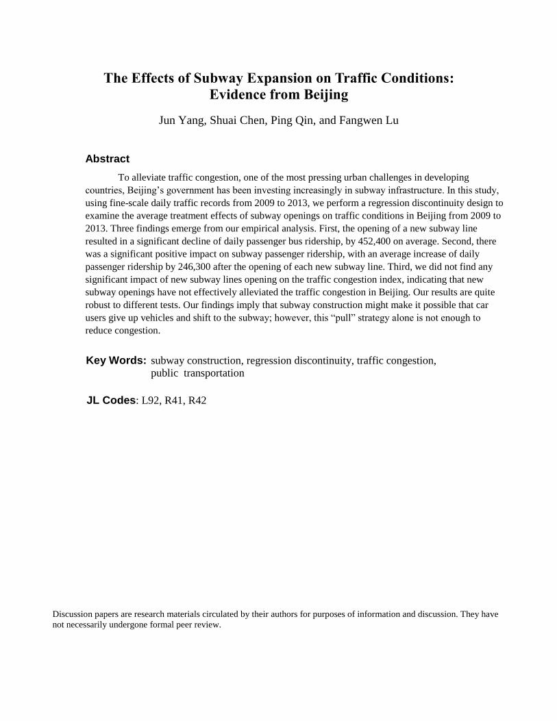
the optimal bandwidth, respectively. The result is shown graphically in Figures 4, 5 and 6. Figure

4 reports the regression results of daily bus and subway ridership under different bandwidths.

The results show that the treatment effects estimation is highly robust in different scenarios,

except for the case of 50% of optimal bandwidth. Figure 5 reports the regression results of the

daily TCI under different bandwidths and Figure 6 reports the results of the morning and evening

peak TCI, respectively. The results were similar to those for bus and subway ridership.

Therefore, we can conclude that our results hold when we choose different bandwidths, except

for 50% of optimal bandwidth.

5.2 Robustness Check with Alternative Polynomial Orders

In our nonparametric estimation with local polynomial regression, we choose the 5th

order term of the forcing variable tX as one of the dependent variables. This section investigates

the robustness of estimation results by choosing other, higher polynomial orders. Table 7 shows

16 Lee and Lemieux (2010) indicated that it is necessary to test the robustness of results under different

specifications of bandwidth h.


14

the estimation results where the 5th, 6th, 7th and 8th order polynomials of tX, respectively, were

controlled based on the benchmark model specification. The results are highly robust among

different polynomial orders. It is noteworthy to mention that the estimation coefficients of the

traffic congestion index were still not significant.

5.3 Robustness Check for Alternative Sample Set

In this section, the samples were re-divided and re-estimated using two kinds of

robustness checks. First, the sample data around the opening date of each subway line was

considered as an independent sample set. Second, we eliminated the sample sets that could be

affected by transportation policies other than subway opening. There were two important

transportation policies introduced in Beijing in our study period. One was a car registration

lottery policy for curbing the total number of cars, beginning on January 1, 2011; the other was

an adjustment of taxi fares on June 10, 2013. As the two points in time fell within our sample

period, the estimation results may be affected. So, we eliminate the sample data around the

opening dates of Line 15 (October 30, 2010) and Line 14 (May 5, 2013), and we re-estimate the

model. The comparison of estimation results for different sample sets is presented in Table 8.

The results of the regression indicate that the opening of each new subway line still had a

significant impact on bus and subway ridership, with the sign of the coefficient as expected.

Moreover, all the marginal effects estimates on the congestion index were insignificant under all

model specifications, except that the marginal effect of Line 14 on the traffic congestion index

during morning and evening peaks showed slight significance, at the 10% confidence level.

After the elimination of the data for Line 15, Line 14, or both, the estimation results of

the ridership of bus and subway were all significant. The sign of the coefficient was the same as

expected. The coefficient estimates of the congestion index were all insignificant and negative,

with the results slightly higher than those under the benchmark condition. In general, the results

of regression estimation remained robust under alternative sample sets.

5.4 Robustness Check at Non-discontinuity Points

As a robustness check of RD design, estimating jumps at points where there should be no

jumps is highly recommended (Imbens and Lemieux 2008). We further perform robustness tests

by artificially choosing cutoffs, which include cutoff 1 at -5 days (5 days before the original

point); cutoff 2 at 5 days (5 days after the original point); cutoff 3 at -10 days (10 days before the

original point); and cutoff 4 at 10 days (10 days after the original point). The estimation results


15

under different configurations of cutoffs are presented in Table 9. In general, the results show

that there are no significant jumps at non-discontinuity points. As to the TCI, only the coefficient

estimates of the evening peak TCI under the configuration of cutoff 1 and the morning peak TCI

under the configuration of cutoff 3 were significant and negative. Therefore, we believe that the

estimation results were basically robust under different configurations of the cutoffs.

5.5 Robustness Check for Various Time-window Lengths of the Sample Data

In the benchmark regression, we chose 60 days before and after the subway line opening

date as a time-window length. Here, we change the time-window length of the samples for

regression discontinuity analysis under the benchmark model, and perform the robustness check

by comparing the estimation results. The samples spanning both 30 and 90 days before and after

the discontinuity point were chosen for estimation (see Fig. 7). It can be seen from Fig. 7 that the

negative impact on bus passenger ridership and the positive impact on subway passenger

ridership still exist for various time-window length sample data. This shows the results’

robustness for sample data covering time windows of various lengths.

5.6 Robustness Check with One Particular Subway Line

We now assess the robustness of our results by looking at the effect on traffic congestion

of only one subway line opening. Ideally, we want information on the traffic congestion index

from one road network to conduct this analysis. However, this type of data is not available. We

instead use the road speed data from Liangguang Street to proxy for the degree of traffic

congestion. The road travels from east to west, with around 8.4 km of its length parallel to Line

7, which opened at the end of 2014. We chose 90 days before and after the Line 7 opening date

as the time-window length. The regression results are presented in Table 10. Our results

demonstrate that there was no significant speed improvement on the Liangguang road network

with the opening of Line 7.

6. Conclusion

As an international metropolitan area under rapid development, Beijing is facing a sharp

rise in its vehicle population. While its residents have enjoyed great benefits from this increase in

mobility, they and their neighbors are also paying a heavy price. Beijing has been named by

numerous international organizations as one of the most gridlocked cities in the world. The city

is also one of the world’s most polluted cities in terms of air quality, and vehicular emissions

contribute heavily to hazardous air pollutants. In order to deal with these challenges, Beijing has


16

invested heavily in public transit infrastructure. According to the Plan for Beijing's Rail Transit

Construction (2011-2020), there will be 30 subway lines constructed by 2020, with around 450

stations and the total length reaching 1,050 kilometers. Although the Beijing government

believes that the expansion of urban rail transit can reduce congestion, pollution and energy

consumption, the potential benefits brought about by rail transit may be overestimated under

actual conditions in Beijing.

We estimate the average treatment effect on bus and subway passenger ridership and

daily congestion indices in Beijing by exploiting the rapid expansion of the subway networks in

recent years. Based on daily passenger ridership information and daily congestion index data, we

use RD design to estimate the impact of the opening of new subway lines on bus and subway

ridership and on the traffic congestion index. We also use a higher order polynomial function to

flexibly control for time-series variation in the ridership or congestion that would have occurred

in the absence of the opening of the subway lines.

We have three major findings. First, a significant and negative impact was found on bus

ridership. On average, the opening of each new subway line resulted in a decline of daily bus

ridership by 452,400. Second, there was a significant positive impact on subway ridership, with

an average increase of daily ridership by 246,300 after the opening of each new subway line.

Third, we did not find a significant impact of new subway lines opening on the traffic congestion

index, including the all-day average index, morning peak index and evening peak index. Though

subway construction makes it possible for car users to give up driving and transfer to the subway

system, our study demonstrates that this “pull” strategy alone is not enough.

We speculate that the low cost of private vehicle use is the main reason that the rapid

expansion of the subway network in Beijing is not effective in reducing traffic congestion. Given

the poor transfer service of the subway system and the crowding of subway cars, especially at

peak times, "door-to-door" commuting using private cars is generally superior to rail transit in

terms of travel speed, comfort, and privacy. In addition, the low cost of private vehicle use

makes it competitive with the subway. According to the 2010 Beijing Household Travel Survey,

the average cost of commuting by private cars was 0.72 yuan/km, only (roughly) five times the

subway cost per km.

It is difficult to attract vehicle owners to give up driving and commute by subway.

Therefore, to reduce traffic congestion, the vigorous development of public transport in Beijing

should be combined with an increase in the cost of using private cars. Otherwise, the potential

benefits from public transport investment will be greatly reduced. For example, some work has


17

shown that vehicle users are fairly sensitive to parking fees. The study by Shoup (2011) in Los

Angeles found that 70% of the commuters would go to the office by private cars when there was

free parking. However, when the parking fee increased to US $5, the proportion declined to 43%,

and the commuters choosing public transport increased markedly. In Beijing and nearly all the

cities in China, free parking is a very common phenomenon. Therefore, it is recommended for

Beijing and other Chinese cities that parking fees be imposed or increased. Combining with the

pull strategy of subway construction, this pull-and-push policy will not only increase the benefits

of subway construction, but also facilitate the shift of commuting modes from private cars to

subway.


18

References

Anderson, M. L. 2014. Subways, Strikes and Slowdowns: The Impact of Public Transit on

Traffic Congestion, American Economic review 104 (9):2763-2796.

Angrist, J. D., and Pischke, J. S. 2008. Mostly Harmless Econometrics: An Empiricist’s

Companion, Princeton: Princeton University Press.

Baum-Snow, N., and M.E. Kahn. 2005. Effects of Urban Rail Transit Expansions: Evidence

from Sixteen Cities, 1970–2000, Brookings-Wharton Papers on Urban Affairs, 147-206.

Washington, D.C.: Brookings Institution Press.

Chen, Y., and A. Whalley. 2012. Green Infrastructure: The Effects of Urban Rail Transit on Air

Quality. American Economic Journal: Economic Policy 4(1): 58-97.

Davis, L.W. 2008. The Effect of Driving Restrictions on Air Quality in Mexico City. Journal of

Political Economy 116(1): 38-81.

Dong, Y., and A. Wu. 2013. The Current Situation of Urban Railway Transit Development in

China. World Railway (7): 36-39 (in Chinese).

Duranton, G., and M. Turner. 2011. The Fundamental Law of Road Congestion: Evidence from

US Cities. American Economic Review 101(6): 2616-2652.

Feng, Y., D. Fullerton, and L. Gan. 2013. Vehicle Choices, Miles Driven and Pollution Policies.

Journal of Regulatory Economics 4(1): 4-29.

Gibbons, S., and S. Machin. 2005. Valuing Rail Access Using Transport Innovations. Journal of

Urban Economics 57(1): 148-169.

Gordon, P., and P. Willson. 1984. The Determinants of Light-rail Transit Demand—An

International Cross-sectional Comparison. Transportation Research Part A 18(2): 135-

140.

Imbens, G., and T. Lemieux. 2008. Regression Discontinuity Design: A Guide to Practice.

Journal of Econometrics 142(2): 615-635.

Kain, J.F., and Z. Liu. 1994. Efficiency and Locational Consequences of Government Transport

Policies and Spending in Chile, Harvard Project on Urbanization in Chile, Harvard

University.

Lee, D.S., and T. Lemieux. 2010. Regression Discontinuity Designs in Economics. Journal of

Economic Literature 48: 281-355.


19

Li, S., J. Yang, P. Qin, and S. Chonabayashi. 2014. Wheels of Fortune: Subway Expansion and

Property Values in Beijing, Working Paper.

Li, S. 2014. Better Lucky than Rich? Welfare Analysis of Vehicle License Restrictions in

Beijing and Shanghai, Working Paper.

Nelson, P., A. Baglino, W. Harrington, E. Safirova, and A. Lipman. 2007. Transit in

Washington, D.C.: Current Benefits and Optimal Level of Provision. Journal of Urban

Economics 62(2): 231-251.

Parry, I., and K.A. Small. 2009. Should Urban Transit Subsidies Be Reduced? American

Economic Review 99(3): 700-724.

Petitte, R. 2001. Fare Variable Construction and Rail Transit Ridership Elasticities: Case Study

of the Washington, D.C., Metrorail System. Transportation Research Record 1753: 102-

110.

Shoup, D. 2011. The High Cost of Free Parking. Chicago: Planners Press.

Sun, C., S.Q. Zheng, and R. Wang. 2014. Restricting Driving for Better Traffic and Clearer

Skies: Did it Work in Beijing? Transport Policy 32: 34-41.

Vickrey, W. 1969. Congestion Theory and Transport Investment. American Economic Review 59

(2): 251-60.

West, S. 2004. Distributional Effects of Alternative Vehicle Pollution Control Policies. Journal

of Public Economics 88: 735-57.

Winston, C., and A. Langer. 2006. The Effect of Government Highway Spending on Road

Users’ Congestion Costs. Journal of Urban Economics 60(3): 463-483.

Xie, L. 2012. Automobile Usage and Urban Rail Transit Expansion, Environment for

Development Initiative Discussion Paper.

Yang, J., Y. Liu, P. Qin, and A. Liu. 2014. A Review of Beijing’s Vehicle Lottery: Short-term

Effects on Vehicle Growth, Congestion, and Fuel Consumption. Energy Policy 75: 157-

166.

Zhong, N. 2015. Superstitious Driving Restriction: Traffic Congestion, Ambient Air Pollution,

and Health in Beijing, Working Paper. https://www.econ.cuhk.edu.hk/dept/seminar/14-

15/2nd-term/JMP_NZ.pdf.

https://www.econ.cuhk.edu.hk/dept/seminar/14-15/2nd-term/JMP_NZ.pdf

https://www.econ.cuhk.edu.hk/dept/seminar/14-15/2nd-term/JMP_NZ.pdf


20

Zhou, H. 2015. Comparative Study of Coordinated Development of Urban Transport and High

Density Functional Areas: A Case Study in Beijing and Tokyo. Modern Urban Research

3: 9-15 (in Chinese).


21

Tables and Figures

Table 1. Sample Subway Lines and Selection of Sample Period

Subway Lines Date Sample Period Stations Length(km) Holidays

Line 4 Sep. 28, 2009 08/17/2009-12/15/2009 24 28.2 8

Line 15 Dec. 30, 2010 10/31/2010-02/28/2011 54 122.4 10

Line 9 Dec. 31, 2011 11/01/2011-02/29/2012 13 16.5 10

Line 6 Dec. 30, 2012 10/31/2012-02/28/2013 20 30.4 10

Line 14 May 5, 2013 03/06/2013-07/04/2013 7 12.4 9

Notes: Total sample N=605. We choose 60 days before and after subway line opening (cutoffs) respectively, which

include 121 days for each subway line. Holidays exclude weekends.

Table 2. Summary Statistics

Variable Unit Mean SD Min Max

Bus Passenger Volume (BPV) Million 13.274 1.757 5.463 15.800

Subway Passenger Volume (SPV) Million 6.278 1.868 1.321 10.370

Traffic Congestion Index (TCI, Daily Average) 0-10 4.568 1.856 1 8.550

Traffic Congestion Index (TCI, Morning Peak) 0-10 3.639 2.064 0.800 9.300

Traffic Congestion Index (TCI, Evening Peak) 0-10 5.450 2.141 1 9.300

Holiday (0, 1) 0.078 0.268 0 1

Extreme Weather (0, 1) 0.035 0.183 0 1

Note: N=605. Other variables in our research include dummies for weekdays and subway lines, respectively. For

brevity, they are not reported here. Holiday excludes weekends; extreme weather includes heat wave, cold spell,

rainstorm, gale and snow, based on meteorological definitions at Baidu Encyclopedia (http://baike.baidu.com/).


22

Table 3. Sharp RDD: Model Specifications (1)-(4)

Model Specification (1) (2) (3) (4)

BPV BPV BPV BPV

Treat -0.7748***

-0.7501***

-0.6984***

-0.4524***

(-6.27) (-7.04) (-5.73) (-6.16)

Predictor -0.0105**

-0.0135***

-0.0120***

-0.0086***

(-3.50) (-6.15) (-3.93) (-6.13)

Interaction 0.0017 0.0007 0.0012 -0.0085**

(0.35) (0.19) (0.34) (-3.03)

Holiday -3.5946***

(-8.14)

Extreme weather -0.3179

(-1.73)

Weighted by stations No Yes Yes Yes

Polynomial in Time trend No No Yes Yes

Covariates No No No Yes

_cons 13.6385***

13.4704***

13.2839***

14.1002***

(63.19) (55.53) (79.89) (114.29)

N 605 605 605 605

R2 0.158 0.194 0.288 0.724

Notes: “Polynomial in Time trend” controls 5th order polynomial in predictor; “Covariates” contain both weekday

dummies and subway lines dummies as extra control variables; Std. Err. adjusted for 7 clusters for the seven days of

the week; t statistics in parentheses; * p < 0.1,

** p < 0.05,

*** p < 0.01.

Table 4. SRD: Baseline Regressions Relative to Model Specification (1)-(4)

BPV SPV TCI(DA) TCI(MP) TCI(EP)

Panel 1 Local Linear Estimation

Treat -0.7748***

-0.0449 -0.4269 -0.4706* -0.4577

(-6.27) (-1.83) (-1.66) (-2.00) (-1.70)

R2 0.158 0.001 0.098 0.054 0.113

Panel 2 Add Weighted Regression by Stations

Treat -0.7501***

0.0724 -0.6050 -0.7794* -0.5876

(-7.04) (1.84) (-1.52) (-1.95) (-1.67)

R2 0.194 0.002 0.182 0.107 0.212

Panel 3 Add Higher-order Polynomial in Predictor

Treat -0.6984***

0.0974 -0.5506 -0.7561 -0.5061

(-5.73) (1.42) (-1.43) (-1.92) (-1.55)

R2 0.288 0.533 0.254 0.151 0.333

Panel 4 Control Holiday, Weekday, Extreme Weather and Subway Lines

Treat -0.4524***

0.2463***

-0.3219 -0.5322 -0.2707

(-6.16) (4.22) (-0.99) (-1.53) (-0.91)

R2 0.724 0.806 0.707 0.697 0.679

Notes: N=605; Panels (1)-(4) correspond to model specifications (1)-(4); Std. Err. adjusted for 7 clusters for the

seven days of the week; t statistics in parentheses; * p < 0.1,

** p < 0.05,

*** p < 0.01.


23

Table 5. Composition of Traffic Flow from 2011-2013

Year Car (%) Taxi (%) Bus (%) Others (%) Total

2011 58.29 16.90 9.61 15.19 100

2012 62.45 14.03 8.60 14.92 100

2013 64.18 13.38 5.24 17.21 100

Data Source: Beijing Traffic Flow Check Survey, 2011-2013. The Beijing Transportation Research Center selected

more than 300 observation points within the 5th Ring Road, and conducted a one-day traffic flow observation

survey.

Table 6. Characteristics of Different Travel Modes

Mode Distance

(km)

Time

(mins)

Velocity

(km/h)

Cost

(RMB/km)

Car 11.5 38.9 17.7 0.07

Subway 18.0 77.3 14.0 0.14

Bus 10.8 65.4 9.9 0.06

Taxi 9.3 39.2 14.2 2.43

Data Source: Beijing Household Travel Survey, 2010.

Table 7. Robustness Check: nth order Polynomial


5th order Polynomial (Baseline)

Treat -0.4524***

0.2463***

-0.3219 -0.5322 -0.2707

(-6.16) (4.22) (-0.99) (-1.53) (-0.91)

R2 0.724 0.806 0.707 0.697 0.679

6th order Polynomial

Treat -0.4511***

0.2466***

-0.3534 -0.5440 -0.3245

(-6.10) (4.05) (-1.07) (-1.53) (-1.05)

R2 0.724 0.806 0.717 0.698 0.700


Treat -0.4782***

0.2530***

-0.3972 -0.5941 -0.3660

(-6.24) (4.06) (-1.13) (-1.57) (-1.12)

R2 0.725 0.807 0.720 0.702 0.702


Treat -0.4641***

0.2210***

-0.3616 -0.5421 -0.3421

(-6.03) (3.74) (-1.03) (-1.47) (-1.02)

R2 0.725 0.809 0.721 0.704 0.702

Notes: N=605; regression based on model specification (4); Std. Err. adjusted for 7 clusters for the seven days of the

week; t statistics in parentheses; * p < 0.1,

** p < 0.05,

*** p < 0.01.


24

Table 8. Robustness Check: Subsample Regressions


Subway Line 4 (Sept. 28, 2009)

Treat -0.2789* 0.4539

*** -0.5303 -0.8148

* -0.2443

(-1.76) (4.83) (-1.06) (-2.34) (-0.35)

N 121 121 121 121 121

R2 0.680 0.665 0.699 0.732 0.562

Subway Line 15 (Dec. 30, 2010)

Treat -0.1490 0.5079***

-0.5896 -1.0014 -0.5197

(-1.04) (5.40) (-0.99) (-1.74) (-0.85)

N 121 121 121 121 121

R2 0.690 0.638 0.778 0.739 0.783


Treat -0.8554***

0.0288 -0.3614 -0.6965 0.0333

(-5.57) (0.25) (-1.10) (-1.43) (0.07)

N 121 121 121 121 121

R2 0.701 0.725 0.709 0.700 0.699


Treat 0.0486 1.0750***

-0.1808 -0.1995 -0.1013

(0.43) (6.28) (-0.24) (-0.26) (-0.13)

N 121 121 121 121 121

R2 0.854 0.804 0.712 0.643 0.665

Subway Line 14 (May 5, 2013)

Treat -0.5828**

-0.1982 -0.5163 -0.2835 -0.6805

(-2.88) (-0.67) (-0.94) (-0.48) (-1.24)

N 121 121 121 121 121

R2 0.820 0.761 0.555 0.667 0.396

Without subway line 15

Treat -0.3060**

0.3681***

-0.3674 -0.6190 -0.3239

(-3.49) (5.53) (-0.86) (-1.51) (-0.80)

N 484 484 484 484 484

R2 0.713 0.805 0.726 0.707 0.698

Without subway line 14

Treat -0.3288**

0.3862***

-0.4187 -0.7013 -0.3469

(-3.29) (4.81) (-0.97) (-1.53) (-0.87)

N 484 484 484 484 484

R2 0.717 0.728 0.739 0.713 0.724

Without both subway lines 15 and 14

Treat -0.5856***

0.2074**

-0.2918 -0.3588 -0.2281

(-9.97) (3.32) (-1.25) (-1.13) (-0.95)

N 363 363 363 363 363

R2 0.764 0.774 0.684 0.682 0.619

Notes: All regressions based on model specification (4); Std. Err. adjusted for 7 clusters for the seven days of the


** p < 0.05,

*** p < 0.01.


25

Table 9. Robustness Check: Choose Cutoff Point Arbitrarily Based on Baseline Model


Cutoff1 Five days before

-0.2765 -0.0742 -0.0320 0.2549 -0.7946**

(-1.02) (-0.37) (-0.09) (0.64) (-1.99)

Cutoff 2 Five days after

0.2361 -0.0577 0.0984 0.1251 -0.5477

(0.94) (-0.28) (0.21) (0.33) (-1.39)

Cutoff3 Ten days before

-0.0865 -0.0122 -0.2272 -0.8568***

0.1778

(-0.39) (-0.07) (-0.77) (-2.66) (0.47)

Cutoff4 Ten days after

0.4484 0.1667 0.1578 0.6219 0.2266

(1.68) (0.76) (0.40) (1.62) (0.55)

Notes: N=605; regression based on model specification (4); Std. Err. adjusted for 7 clusters for the seven days of the


** p < 0.05,

*** p < 0.01.

Table 10. Robustness Check: Road Speed along Subway Line 7

Subway Line 7 (Dec.28 2014)

City level variables BPV SPV TCI(MP) TCI(EP)

Treat -0.4729**

0.1401 -0.0104 0.0944

(-2.77) (0.35) (-0.04) (0.26)

R2 0.848 0.663 0.717 0.663

Speed around Line 7 WtE(MP) WtE(EP) EtW(MP) EtW(MP)

Treat 0.7461 0.0467 0.6441 -0.2083

(1.39) (0.07) (1.56) (-0.25)

R2 0.665 0.642 0.594 0.640

Notes: N=212, Obs. from 2014-09-01 to 2015-03-31; t statistics in parentheses; * p < 0.1,

** p < 0.05,

*** p < 0.01.

WtE and EtW indicate west-east and east-west direction, and MP and EP indicate morning peak (7:00-9:00am) and

evening peak (17:00-19:00).


26

Figure 1. Map of Sample Subway Lines in Beijing

Figure 2. Local Linear vs. Polynomial in Bus Ridership RD.

Notes: The estimated change in BPV just after the subway opening is -0.4524 (million) and is statistically significant

(95% CI: -0.6321, -0.2727).

68

10

12

14

16

BP

V (

mill

ion)

-50 0 50

Predictor (days)

68

10

12

14

16

BP

V (

mill

ion)

-50 0 50

Predictor (days)


27

Figure 3. Local Linear vs. Polynomial in Subway Ridership RD

Notes: The estimated change in SPV just after the subway opening is 0.2463 (million) and is statistically significant

(95% CI: 0.1034, 0.3893).

Figure 4. Change Bandwidth for Local Polynomial Smoothing in Bus and Subway Ridership

Notes: Gray bars indicate 95% CI at corresponding bandwidth.

24

68

SP

V (

mill

ion)

-50 0 50

Predictor (days)

24

68

SP

V (

mill

ion)

-50 0 50

Predictor (days)

-.2

-.4

0.2

-.6

-.8

The E

stim

ate

d C

hanges in B

PV

(m

illio

n)

10050 75 125 150 175 200

Bandwidth (%)

0

.25

.5.7

5

The E

stim

ate

d C

hanges in S

PV

(m

illio

n)

10050 75 125 150 175 200

Bandwidth (%)


28

Figure 5. Polynomial and Bandwidth in TCI (DA).

Notes: The estimated change in TCI (DA) just after the subway opening is -0.3219 (index) and is statistically

insignificant with any bandwidth (95% CI:-1.1141, 0.4704).

Figure 6. Polynomial and Bandwidth in TCI (MP) and TCI (EP), Respectively

02

46

8

TC

I (D

aily

Avera

ge)

-50 0 50

Predictor (days)

-2-1

01

2

The E

stim

ate

d C

hanges in T

CI(

DA

)

10050 75 125 150 175 200

Bandwidth (%)

10

-1-2

-3

The E

stim

ate

d C

hanges in T

CI(

MP

)

10050 75 125 150 175 200

Bandwidth (%)

0-1

-.5

.51

1.5

The E

stim

ate

d C

hanges in T

CI(

EP

)

10050 75 125 150 175 200

Bandwidth (%)


29

Figure 7. Robustness Check in Bus and Subway Ridership by Alternative Sample Selections: Change Sample Period from [-60, 60] to [-30, 30] and [-90, 90]. ([-60, 60] is our

Baseline)

68

10

12

14

16

BP

V (

mill

ion)

-30 -20 -10 0 10 20 30

Predictor (days)

24

68

10

SP

V (

mill

ion)

-30 -20 -10 0 10 20 30

Predictor (days)

68

10

12

14

16

BP

V (

mill

ion)

-50 0 50

Predictor (days)

24

68

SP

V (

mill

ion)

-50 0 50

Predictor (days)

05

10

15

BP

V (

mill

ion)

-90 -60 -30 0 30 60 90

Predictor (days)

24

68

10

12

SP

V (

mill

ion)

-90 -60 -30 0 30 60 90

Predictor (days)

Documents

The Effects of Subway Expansion on Traffic Conditions ... · PDF fileEnvironment for Development Discussion Paper Series August 2015 EfD DP 15-22 The Effects of Subway Expansion on