The Effect of Workplace Inspections on Worker Safety

Ling Li and Perry Singleton

Paper No. 201 February 2017

CENTER FOR POLICY RESEARCH –Spring 2017

Leonard M. Lopoo, Director Professor of Public Administration and International Affairs (PAIA)

Associate Directors Margaret Austin

Associate Director, Budget and Administration

John Yinger Trustee Professor of ECON and PAIA

Associate Director, Metropolitan Studies

SENIOR RESEARCH ASSOCIATES

Badi Baltagi, ECON Robert Bifulco, PAIA Leonard Burman, PAIA Thomas Dennison, PAIA Alfonso Flores-Lagunes, ECON Sarah Hamersma, PAIA Madonna Harrington Meyer, SOC William Horrace, ECON Yilin Hou, PAIA

Jeffrey Kubik, ECON Yoonseok Lee, ECON Amy Lutz, SOC Yingyi Ma, SOC Katherine Michelmore, PAIA Jerry Miner, ECON Cynthia Morrow, PAIA Jan Ondrich, ECON

David Popp, PAIA Stuart Rosenthal, ECON Michah Rothbart, PAIA Rebecca Schewe, SOC Amy Ellen Schwartz, PAIA/ECON Perry Singleton, ECON Michael Wasylenko, ECON Peter Wilcoxen, PAIA

GRADUATE ASSOCIATES

Alejandro Alfaro Aco, PAIA Emily Cardon, PAIA Ziqiao Chen, PAIA Jena Daggett, PAIA Alex Falevich, ECON Wancong Fu, ECON Emily Gutierrez, PAIA Jeehee Han, PAIA Boqian Jiang, ECON

Hyunseok Jung, ECON Khatami, Seyedvahid, IR Yusun Kim, PAIA Ling Li, ECON Michelle Lofton, PAIA Judson Murchie, PAIA Brian Ohl, PAIA Jindong Pang, ECON Krushna Ranaware, SOC

Laura Rodriquez-Ortiz, PAIA Fabio Rueda De Vivero, ECON David Schwegman, PAIA Shulin Shen, ECON Iuliia Shybalkina, PAIA Kelly Stevens, PAIA Saied Toossi, PAIA Rebecca Wang, SOC Xirui Zhang, ECON

STAFF

Kathleen Nasto, Administrative Assistant Candi Patterson, Computer Consultant Mary Santy, Administrative Assistant

Laura Walsh, Administrative Assistant Katrina Wingle, Administrative Specialist

Abstract The Occupation Safety and Health Administration enforces safety regulations through workplace

inspections. To identify the effect of inspections on worker safety, this study exploits quasi-

experimental variation in inspections due to OSHA’s Site Specific Targeting plan. The SST plan

used establishment-level data on accidents and injuries to target establishments for inspection.

The primary inspection list consisted of establishments with case rates exceeding a cutoff. This

cutoff generated a discontinuous increase in inspections, which is used to identify the effect of

inspections on worker safety. Using the fuzzy regression discontinuity design and local linear

regression, the estimated effect of an inspection on cases involving days away from work, job

restrictions, and job transfers is -1.607 per 100 full-time equivalent workers. The effect is most

pronounced among manufacturing establishments below the 90th percentile of the case-rate

distribution.

JEL No. J28; K32

Keywords: OSHA; Worker Safety; Regression Discontinuity

Authors: Ling Li, Department of Economics, Center for Policy Research, Syracuse University;

Perry Singleton, Associate Professor, Department of Economics, Senior Research Associate,

Center for Policy Research, Syracuse University.

Acknowledgement: For valuable comments, the authors thank Gary Engelhardt, Alfonso

Flores-Lagunes, Hugo Jales, and Jeffrey Kubik.

I. Introduction

In 2016, the Occupational Safety and Health Administration conducted approximately 32

thousand workplace inspections, with a fiscal year budget of $553 million. While the goal of

inspections is to enforce federal regulations of safety and health, identifying the effect of

inspections on worker safety presents a challenge. One reason is that OSHA specifically targets

high-risk industries and establishments for inspection (Kniesner and Leeth 2014). This generates

a negative correlation between inspections and worker safety, which confounds any positive,

causal effect of the former on the latter.

To identify the effect of inspections on worker safety, this study exploits quasi-experimental

variation in inspections generated by OSHA’s Site Specific Targeting (SST) plan. The plan,

implemented in 1999, targeted establishments with high rates of accidents and injuries for

inspection. The data to implement the SST plan come from the OSHA Data Initiative (ODI), which

collected establishment-level data on accidents and injuries directly from employers. Using these

data, the SST plan prioritized establishments for inspection using case-rate cutoffs. One set of

cutoffs defined the primary inspection list, and a lower set of cutoffs defined the secondary

inspection list. An even lower cutoff was used to notify employers by mail that their case rates

were high relative to the national average. The cutoff for the primary inspection list is associated

with a discontinuous increase in inspections, which is used to identify the effect of inspections

on worker safety.

To exploit the discontinuity in inspection for identification, the empirical strategy follows the

fuzzy regression discontinuity (FRD) design (Hahn, Todd, and Van der Klaauw 2001; Imbens and

Lemieux 2008). The FRD design requires that establishments are similar just above and below the

cutoff, and that the discontinuity in inspection is due to compliers, defined as establishments

1

that were inspected just above the cutoff, but would have not have been inspected in the

absence of the SST plan. These assumptions are supported by examining establishment

characteristics and inspections unrelated to the SST plan. If the identification assumptions are

valid, the FRD estimand measures the average effect of an inspection among compliers at the

cutoff. The study also examines whether the effect of an inspection varies across the distribution

of worker safety outcomes. This will determine whether the average effect of an inspection

among compliers, estimated using the FRD estimand, varies between establishments with high

versus low case rates after the SST plan. The estimands for distributional effects come from

Frandsen, Frolich, and Melly (2012). To estimate both the mean and distributional effects, the

empirical strategy uses a robust, bias-correction procedure developed by Calonico, Cattaneo, and

Titiunik (2014).

The primary data come from OSHA’s Data Initiative (ODI), conducted annually from 1996 to

2011. The data report the employer name, establishment address, and industry. In regards to

accidents and injuries, the data report the total case rate (TCR) and the DART rate. The TCR

includes cases involving (1) death, (2) days away from work, (3) job transfers or restrictions, or

(4) medical attention beyond first aid, whereas the DART rate excludes cases involving death and

medical attention beyond first aid. These rates are calculated annually per 100 full-time

equivalent workers. The ODI data are used to determine both the proximity to the inspection-list

cutoff before the SST plan, as well as worker safety outcomes following the SST plan. Thus, the

data are restricted to establishments observed at least twice, with two observations spaced four

years apart.1 To determine inspection outcomes during the SST plan, the ODI data are linked to

OSHA’s Integrated Management Information System. To determine union activity within an

1 While the ODI data were not designed as a panel, many establishments are observed in the ODI in multiple years.

2

establishment, the ODI data are linked to “notices of bargaining” filed with the Federal Mediation

and Conciliation Service.2

The empirical analysis focuses on the DART rate cutoff for the primary inspection list. Using

local linear regression, this cutoff is associated with a 22.7 percentage point increase in

“programmed” inspections, a 17.5 percentage point increase in any citations, and a 15.4

percentage point increase in penalties. The cutoff is not associated with a change in

“unprogrammed” inspections, which are unrelated to the SST plan. Thus, the SST plan provides a

sizeable discontinuity in inspections for identification.

The effect of inspection on worker safety is most evident for the DART rate. Using the FRD

design and local linear regression, the average effect of an inspection on the DART rate among

compliers is -1.607 per 100 full-time equivalent workers. This estimate is statistically significant

at the five percent level and robust to the inclusion of establishment characteristics. Moreover,

the effect on the DART rate is most pronounced among manufacturing establishments below the

90th percentile of the DART distribution post-inspection. Treatment effects are less evident for

other case rates, such as the TCR, and for other industries. Treatment effects also do not differ

significantly between union and non-union establishments, suggesting that unionization is

neither a substitute nor a complement to workplace inspections.3

This study contributes to a literature on the effects of OSHA inspections on worker safety. In

general, most studies find little to no “abatement” effect of inspections on worker safety, and

studies that do find an effect may suffer from confounding biases (Kniesner and Leeth 2004).4

2 DiNardo and Lee (2004) use “notices of bargaining” filed with the Federal Mediation and Conciliation Service to determine union activity following a union vote. 3 The effect of unionization on worker safety has been examined by Morantz (2009, 2013). 4 Studies in this literature include Cooke and Gautschi (1981); Gray and Scholz (1993); Gray and Mendeloff (2005); Haviland et al. (2010); McCaffrey (1983); and Ruser and Smith (1991). The little to no effect of an OSHA inspection

3

These studies differ by the analysis period, the definition of treatment (inspection versus citation

or penalty), and worker safety outcome (overall injuries versus specific accidents). To address

selection bias, some studies exploit the timing of an inspection, arguing that establishments

inspected earlier in the year have more time to remediate workplace hazards. One study, by

Levine, Toffel, and Johnson (2012), use experimental data from California in 1996 to 2006. By

exploiting random assignment of inspections among 409 establishments, they find that

inspections reduce injuries by 9.4 percent, with no detectable effect on employment, sales, or

firm survival. However, their sample was limited to high-risk industries in California, so their

findings may not be generalizable to other industries or US states.

The estimates from this study appear at the high end of effects. Relative to the average DART

rate at the cutoff, the average effect of -1.607 amounts to a 20 percentage point reduction in

injuries. However, this estimate pertains only to compliers near the cutoff, which is located at

85th percentile of the DART distribution pre-inspection. While this suggests that the effect of an

inspection on worker safety may be greater among high-risk firms, the effect is concentrated

below the 90th percentile of the DART distribution post-inspection. This study also differs from

related studies with respect to the data and analysis sample. Thus, it is difficult to reconcile the

estimates of this study with those of the related literature.5 In regards to efficiency, the gains

from reducing the DART rate at the cutoff are offset by the cost of an inspection for OSHA and

the cost of compliance for employers.

on worker safety may reflect that OSHA penalties are too low (Viscusi 1979) or that safety and health standards are not directly related to workplace accidents (Bartel and Glenn 1985). 5 A report by Summit Consulting (Peto et al. 2016) pursues a similar identification strategy as this study, but this report uses ODI data collected in 2007 only. They find small and statistically insignificant effects of an inspection on worker safety. A qualitatively similar result is obtained in this study when the data are restricted to the ODI data collected in 2007 (not shown).

4

II. Background

The goal of the Occupational Safety and Health Act, passed by the US Congress in 1970, is “to

assure safe and healthful working conditions for working men and women.” To achieve this goal,

the Occupational Safety and Health Administration (OSHA) was created to codify and enforce

safety and health regulations. Regulations include specification standards, such as requiring

safety guards for machinery or equipment, as well as performance standards, such as requiring

limits on exposure to hazardous chemicals (Kniesner and Leeth 2014). To enforce regulations,

OSHA educates employers and employees, inspects worksites for workplace hazards, and levies

financial penalties on employers for serious or repeated violations.

OSHA inspections are either programmed or unprogrammed. Unprogrammed inspections

result from fatal or catastrophic accidents, employee complaints, or referrals, while programmed

inspections are intended to identify and abate workplace hazards before an accident or illness

occurs. In fiscal year 2015, OSHA conducted 16,527 programmed inspections and 19,293

unprogrammed inspections.6 Among unprogrammed inspections, 912 were due to fatal or

catastrophic accidents, 9,037 were due to employee complaints, 4,705 were due to referrals, and

4,639 were due to other reasons.

In 1999, OSHA drastically changed its procedure for targeting programmed inspections.

Before 1999, programmed inspections were targeted at industries with high rates of accidents

and injuries. This was accomplished using industry-level data collected by the Bureau of Labor

Statistics. However, after an inspection, many establishments in high-risk industries were found

to be relatively safe. Thus, targeting high-risk industries was relatively inefficient at targeting

high-risk establishments, since worker safety varied substantially within industries.

6 These figures exclude State Plan inspections, which totaled 43,105 in fiscal year 2016.

5

To better target high-risk establishments, OSHA created the OSHA Data Initiative (ODI) in

1996. The goal of the ODI was to collect data on accidents and injuries directly from employers

at the establishment level. The ODI survey was conducted annually from 1997 to 2011, with

approximately 80,000 establishments surveyed each year. The survey covers manufacturing and

industries with injury rates above the national average, except construction, and excludes

establishments with fewer than 40 employees.7 To facilitate data collection, OSHA required

establishments to record accidents and injuries using OSHA’s Form 300. Per the form, cases must

be recorded if they involve death, days away from work, job transfers or restrictions, or medical

attention beyond first aid. These data were then used to calculate case rates for the calendar

year. The DAFWII includes cases involving days away from work; the DART includes cases

involving days away from work and job transfers or restrictions, and the TCR includes all case

types, including death.8 These rates are calculated and reported per 100 full-time equivalent

workers.9

The ODI data were then used to implement OSHA’s Site-Specific Targeting (SST) plan. The goal

of the SST plan was to target programmed inspections at establishments with high rates of

accidents and injuries. To target high-rate establishments, the SST plan prioritized establishments

using case-rate cutoffs. For example, the ODI in 2003 collected case-rate data for calendar year

2002, and the SST plan used these data to target programmed inspections from April 2004 to

August 2005. The primary inspection list included establishments with a DART rate greater than

15 or a DAFWII rate greater than 10. A secondary inspection list included establishments with a

7 In 1999, the ODI excluded establishments with fewer than 60 employees. 8 In 2002, DART replaced LWDII due to a change in recordkeeping. The LWDII includes only cases involving lost work days due to injury or illness and is nearly identical to DART. 9 To calculate case rates, the ODI asks employers to report the number of employees and the total hours worked by employees during the previous calendar year. This information is not reported in the ODI data.

6

DART rate greater than 10 or a DAFWII rate greater than 4. Additionally, all establishments with

a DART rate greater than 7 were mailed a letter stating that their DART rates were high relative

to the national average. Occasionally, the case-rate cutoffs changed, reflecting changes in the

case-rate distribution and OSHA’s resources to conduct inspections. While all establishments on

the primary list were targeted for an inspection, only 20 percent were ultimately inspected, and

those that were inspected did not always have the highest case rates (US Department of Labor

2012). The low inspection rate was attributed, in part, to limited resources (US Department of

Labor 2012).

III. Methodology

The empirical objective is to identify the causal effect of an OSHA inspection on worker safety.

The effect is identified using quasi-experimental variation in inspections generated by OSHA’s

SST plan. Specifically, the SST established a case-rate cutoff, and establishments exceeding the

cutoff were targeted for a programmed inspection. If this process generated a discontinuous

increase in inspections at the cutoff, and if establishments just above and below the cutoff are

similar, then the increase in inspections at the cutoff may be used to identify the causal effect of

an inspection on worker safety.

A. Fuzzy Regression Discontinuity

The empirical strategy utilizes the fuzzy regression discontinuity (FRD) design (Hahn, Todd,

and Van der Klaauw 2001; Imbens and Lemieux 2008) using the potential outcomes framework

of Rubin (1974) and Holland (1986). Using this framework, each establishment has two potential

outcomes: worker safety without an OSHA inspection, denoted 𝑌𝑌𝑖𝑖(0), and worker safety with an

OSHA inspection, denoted 𝑌𝑌𝑖𝑖(1). For each establishment, the causal effect of an OSHA inspection

7

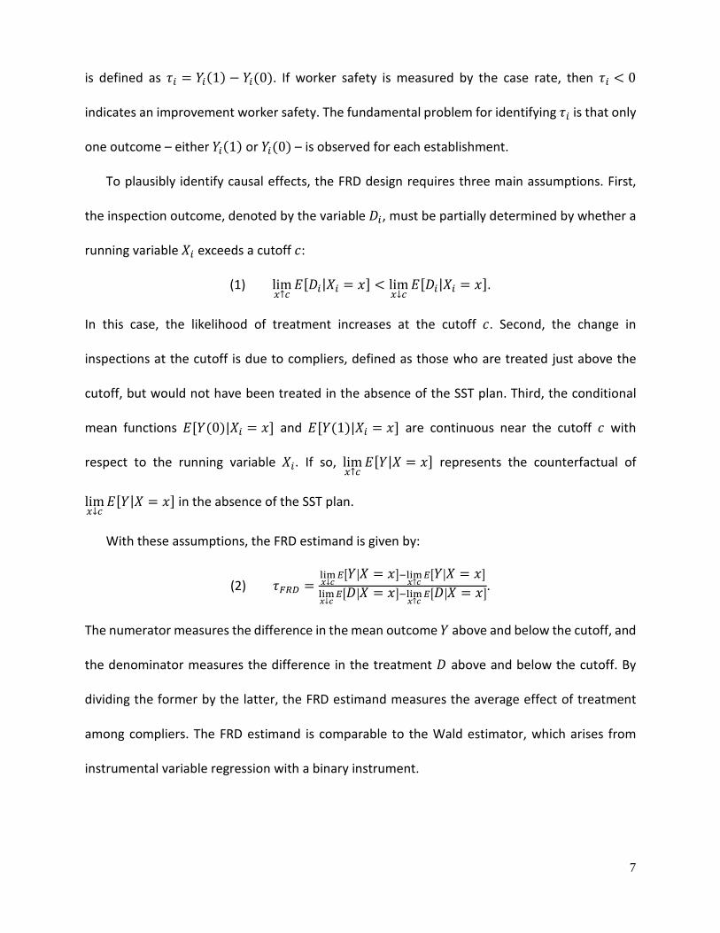
is defined as 𝜏𝜏𝑖𝑖 = 𝑌𝑌𝑖𝑖(1) − 𝑌𝑌𝑖𝑖(0). If worker safety is measured by the case rate, then 𝜏𝜏𝑖𝑖 < 0

indicates an improvement worker safety. The fundamental problem for identifying 𝜏𝜏𝑖𝑖 is that only

one outcome – either 𝑌𝑌𝑖𝑖(1) or 𝑌𝑌𝑖𝑖(0) – is observed for each establishment.

To plausibly identify causal effects, the FRD design requires three main assumptions. First,

the inspection outcome, denoted by the variable 𝐷𝐷𝑖𝑖, must be partially determined by whether a

running variable 𝑋𝑋𝑖𝑖 exceeds a cutoff 𝑐𝑐:

(1) lim𝑥𝑥↑𝑐𝑐

𝐸𝐸[𝐷𝐷𝑖𝑖|𝑋𝑋𝑖𝑖 = 𝑥𝑥] < lim𝑥𝑥↓𝑐𝑐

𝐸𝐸[𝐷𝐷𝑖𝑖|𝑋𝑋𝑖𝑖 = 𝑥𝑥].

In this case, the likelihood of treatment increases at the cutoff 𝑐𝑐. Second, the change in

inspections at the cutoff is due to compliers, defined as those who are treated just above the

cutoff, but would not have been treated in the absence of the SST plan. Third, the conditional

mean functions 𝐸𝐸[𝑌𝑌(0)|𝑋𝑋𝑖𝑖 = 𝑥𝑥] and 𝐸𝐸[𝑌𝑌(1)|𝑋𝑋𝑖𝑖 = 𝑥𝑥] are continuous near the cutoff 𝑐𝑐 with

respect to the running variable 𝑋𝑋𝑖𝑖. If so, lim𝑥𝑥↑𝑐𝑐

𝐸𝐸[𝑌𝑌|𝑋𝑋 = 𝑥𝑥] represents the counterfactual of

lim𝑥𝑥↓𝑐𝑐

𝐸𝐸[𝑌𝑌|𝑋𝑋 = 𝑥𝑥] in the absence of the SST plan.

With these assumptions, the FRD estimand is given by:

(2) 𝜏𝜏𝐹𝐹𝐹𝐹𝐹𝐹 =lim𝑥𝑥↓𝑐𝑐

𝐸𝐸�𝑌𝑌�𝑋𝑋 = 𝑥𝑥�−lim𝑥𝑥↑𝑐𝑐

𝐸𝐸�𝑌𝑌�𝑋𝑋 = 𝑥𝑥�lim𝑥𝑥↓𝑐𝑐

𝐸𝐸�𝐷𝐷�𝑋𝑋 = 𝑥𝑥�−lim𝑥𝑥↑𝑐𝑐

𝐸𝐸�𝐷𝐷�𝑋𝑋 = 𝑥𝑥�.

The numerator measures the difference in the mean outcome 𝑌𝑌 above and below the cutoff, and

the denominator measures the difference in the treatment 𝐷𝐷 above and below the cutoff. By

dividing the former by the latter, the FRD estimand measures the average effect of treatment

among compliers. The FRD estimand is comparable to the Wald estimator, which arises from

instrumental variable regression with a binary instrument.

8

B. Distributional Effects

The FRD estimand measures the average treatment effect of among compliers. However, the

effect among compliers may differ across the distribution of the outcome variable 𝑌𝑌. On one

hand, establishments with high 𝑌𝑌, which are presumably more dangerous, have greater scope

for remediating workplace hazards. On the other hand, these establishments may face greater

idiosyncratic risk beyond the purview of OSHA regulations and enforcement. Thus, the effect of

an inspection across the distribution of the outcome variable 𝑌𝑌 is ambiguous.

To estimate distributional effects, the cumulative density function (CDF) for 𝑌𝑌 is estimated

among compliers just above the cutoff, where they are treated, and among counterfactual

compliers just below the cutoff, where they are not treated. The estimands for the conditional

CDFs are provided by (Frandsen, Frolich, and Melly 2012). Above the cutoff, the conditional CDF

is given by:

(3) 𝐹𝐹𝑌𝑌(1)|Ω(𝑦𝑦) =lim𝑥𝑥↓𝑐𝑐

𝐸𝐸�1(𝑌𝑌 ≤ 𝑦𝑦)𝐷𝐷�𝑋𝑋 = 𝑥𝑥�−lim𝑥𝑥↑𝑐𝑐

𝐸𝐸�1(𝑌𝑌 ≤ 𝑦𝑦)𝐷𝐷�𝑋𝑋 = 𝑥𝑥�lim𝑥𝑥↓𝑐𝑐

𝐸𝐸�𝐷𝐷�𝑋𝑋 = 𝑥𝑥�−lim𝑥𝑥↑𝑐𝑐

𝐸𝐸�𝐷𝐷�𝑋𝑋 = 𝑥𝑥� .

Below the cutoff, the conditional CDF is given by:

(4) 𝐹𝐹𝑌𝑌(0)|Ω(𝑦𝑦) =lim𝑥𝑥↓𝑐𝑐

𝐸𝐸�1(𝑌𝑌 ≤ 𝑦𝑦)(1− 𝐷𝐷)�𝑋𝑋 = 𝑥𝑥�−lim𝑥𝑥↑𝑐𝑐

𝐸𝐸�1(𝑌𝑌 ≤ 𝑦𝑦)(1 − 𝐷𝐷)�𝑋𝑋 = 𝑥𝑥�lim𝑥𝑥↓𝑐𝑐

𝐸𝐸�1 − 𝐷𝐷�𝑋𝑋 = 𝑥𝑥�−lim𝑥𝑥↑𝑐𝑐

𝐸𝐸�1 − 𝐷𝐷�𝑋𝑋 = 𝑥𝑥� .

Both CDFs are conditional on compliers, denoted by Ω. At each value of 𝑌𝑌 = 𝑦𝑦, the distributional

impact of treatment among compliers is measured by 𝐹𝐹𝑌𝑌(1)|Ω(𝑦𝑦) − 𝐹𝐹𝑌𝑌(0)|Ω(𝑦𝑦).

C. Estimation

Treatment effects are estimated using nonparametric, local linear regression. Local linear

regression is appropriate because the estimands are evaluated at the cutoff, and because the

9

cutoff is located at the boundary of the bandwidth (Imbens and Lemieux 2008). The term

lim𝑥𝑥↓𝑐𝑐

𝐸𝐸[𝑌𝑌|𝑋𝑋 = 𝑥𝑥] is estimated by solving

(5) min𝛼𝛼𝑌𝑌𝑌𝑌,𝛽𝛽𝑌𝑌𝑌𝑌

∑ �𝑌𝑌𝑖𝑖 − 𝛼𝛼𝑌𝑌𝐹𝐹 − 𝛽𝛽𝑌𝑌𝐹𝐹(𝑋𝑋𝑖𝑖 − 𝑐𝑐)�2Κ �𝑋𝑋𝑖𝑖−𝑐𝑐

ℎ𝑌𝑌𝑌𝑌�𝑐𝑐≤𝑋𝑋𝑖𝑖≤𝑐𝑐+ℎ𝑌𝑌𝑌𝑌 .

The outcome 𝑌𝑌𝑖𝑖 is a linear function of 𝑋𝑋𝑖𝑖 − 𝑐𝑐, with 𝛼𝛼𝑌𝑌𝐹𝐹 as the intercept and 𝛽𝛽𝑌𝑌𝐹𝐹 as the slope. The

objective is to minimize the sum of the squared deviations of 𝑌𝑌𝑖𝑖 from the linear function,

weighted by the kernel function Κ �𝑋𝑋𝑖𝑖−𝑐𝑐ℎ𝑌𝑌𝑌𝑌

�, using observations within the bandwidth of length ℎ𝑌𝑌𝐹𝐹,

from 𝑐𝑐 to 𝑐𝑐 + ℎ𝑌𝑌𝐹𝐹. The solution to the minimization problem is denoted by 𝛼𝛼�𝑌𝑌𝐹𝐹 and �̂�𝛽𝑌𝑌𝐹𝐹, so the

estimate of 𝑌𝑌 given 𝑋𝑋 is 𝛼𝛼�𝑌𝑌𝐹𝐹 + �̂�𝛽𝑌𝑌𝐹𝐹(𝑋𝑋 − 𝑐𝑐), and the estimate of lim𝑥𝑥↓𝑐𝑐

𝐸𝐸[𝑌𝑌|𝑋𝑋 = 𝑥𝑥] is 𝛼𝛼�𝑌𝑌𝐹𝐹. Similarly,

lim𝑥𝑥↑𝑐𝑐

𝐸𝐸[𝑌𝑌|𝑋𝑋 = 𝑥𝑥] is estimated by solving

(6) min𝛼𝛼𝑌𝑌𝑌𝑌,𝛽𝛽𝑌𝑌𝑌𝑌

∑ �𝑌𝑌𝑖𝑖 − 𝛼𝛼𝑌𝑌𝑌𝑌 − 𝛽𝛽𝑌𝑌𝑌𝑌(𝑋𝑋𝑖𝑖 − 𝑐𝑐)�2Κ �𝑋𝑋𝑖𝑖−𝑐𝑐

ℎ𝑌𝑌𝑌𝑌�𝑐𝑐−ℎ𝑌𝑌𝑌𝑌≤𝑋𝑋𝑖𝑖<𝑐𝑐 .

The terms lim𝑥𝑥↓𝑐𝑐

𝐸𝐸[𝐷𝐷|𝑋𝑋 = 𝑥𝑥] and lim𝑥𝑥↑𝑐𝑐

𝐸𝐸[𝐷𝐷|𝑋𝑋 = 𝑥𝑥] are estimated by replacing 𝑌𝑌 with 𝐷𝐷.

The estimation is accomplished using a robust, bias-correction procedure developed by

Calonico, Cattaneo, and Titiunik (2014). This procedure determines the optimal bandwidth ℎ,

corrects for the bias of �̂�𝜏𝐹𝐹𝐹𝐹𝐹𝐹 when estimated using local linear regression, and calculates robust

standard errors that reflect that the bias correction is stochastic. The procedure also allows for

controls for observable characteristics. The optimal bandwidth is calculated for the outcome 𝑌𝑌,

assuming ℎ𝑌𝑌𝑌𝑌 = ℎ𝑌𝑌𝐹𝐹, and this bandwidth is used for the inspection outcome 𝐷𝐷. The default for

the kernel function Κ(. ) is triangular.

IV. Data

The primary data come from OSHA’s Data Initiative (ODI). Stated above, the ODI collected

data on accidents and injuries at the establishment level from 1996 to 2011. The data report the

10

establishment name and address, including the street number, street name, city, state, and zip

code. The data also report the establishment’s industry using the Standard Industrialization

Classification codes (SIC). In regards to accidents and injuries, the data report the TCR, the DART,

and the DAFWII, though the DAFWII is only available for calendar years 2002 and beyond.

The empirical analysis focuses on the DART cutoff for the primary inspection list, so the

running variable 𝑋𝑋𝑖𝑖 is measured by the DART rate reported in the ODI. While the SST plan had

multiple cutoffs for the primary and secondary inspection lists, only the DART cutoff exhibits a

sizeable discontinuity in inspections. Alternative cutoffs are discussed in section VII.

The inspection indicator 𝐷𝐷𝑖𝑖 is obtained by merging the ODI data to the universe of OSHA

inspections as of September, 2016.10 These data come from OSHA’s Integrated Management

Information System. For each inspection, the data report whether the inspection was

programmed or unprogrammed, the citations recorded during the inspection, and the penalties

levied for each citation, if any. The inspection indicator 𝐷𝐷𝑖𝑖 is measured within the SST plan cycle.

For example, the ODI in 2003 collected case-rate data for calendar year 2002, and the SST plan

used these data to target programmed inspections from April 2004 to August 2005. Thus, for that

cycle, 𝐷𝐷𝑖𝑖 measures inspection outcomes from April 2004 to August 2005.

The outcome variable 𝑌𝑌𝑖𝑖 is measured from the ODI in the calendar year after the SST cycle. In

the example above, inspections under the SST plan occurred from April 2004 to August 2005, so

𝑌𝑌𝑖𝑖 is the case rate in the ODI data in 2006. While the ODI data were not designed as a panel, many

establishments are observed in the ODI in multiple years.

The covariates 𝑍𝑍𝑖𝑖 include sets of dummy variables for calendar year, state, industry, and an

indicator of union activity. State and industry are reported in the ODI. Using the SIC codes,

10 The merging procedure is described in the Appendix.

11

industry is categorized into three groups: manufacturing (SIC 20 to 39), health services (SIC 80),

and other. To obtain information on union activity, the ODI data are merged to “notices of

bargaining” filed with the Federal Mediation and Conciliation Service (FMCS). A notice must be

filed to modify a union contract and thus indicate union activity within an establishment. The

FMCS data include all notices filed from 2004 to 2016. The data report the date of the notice and

the name and address of the establishment, including the street number, street name, city, state,

and zip code. Using the FMCS data, a union indicator variable is created that equals one if there

is any union activity and zero otherwise.

The steps used to match the ODI to the IMIS and the FMCS are discussed in the Appendix.

V. Sample

The analysis sample is derived from the ODI using five restrictions. First, the data are

restricted to years 1997 to 2011, since ODI data in 1996 were not used to implement the SST

plan. The pooled data contain 951,077 observations for 328,751 establishments. Second,

observations are excluded if they appear to duplicate a record or if the establishment’s name and

address are missing, eliminating 0.44 percent of the sample. Third, the data are stacked by

establishment by year, and the sample is restricted to pairs of observations spaced four years

apart. This yields 225,215 observation pairs, with the first year ranging from 1997 to 2007. Fourth,

the data are restricted to states covered by the SST plan, which includes all states under federal

jurisdiction with respect to OSHA and a few states that are not. In total, twenty-seven states were

covered by the SST plan throughout the analysis period, and an additional eight states were

covered at some point during the analysis period. Finally, observations pairs are excluded if the

case rate from the ODI is missing or exceeds 100, eliminating 1.9 percent of the sample. The

resulting analysis sample contains 154,808 observation pairs.

12

Table 1 presents summary statistics of the analysis sample. The first column reports statistics

for the entire sample; the second column reports statistics for establishments with DART rates

from four below the cutoff to four above the cutoff; and the last two columns divide

establishments into those just below and above the SST cutoff.

As shown, the SST cutoff is located near the top of the DART rate distribution. Among all

establishments, the mean DART rate is 7.33, and the mean SST cutoff is 13.67. To illustrate the

distribution, Figure 1 plots the distribution of the DART relative to the SST. The distribution is

skewed to the right, and the cutoff is located near the 85th percentile. This means that, in this

study, compliers are relatively high-risk firms. Additionally, the density is smooth near the

cutoff.11 This suggests that establishments do not bunch just below the cutoff to avoid inspection,

which could potentially violate the identification assumption that establishments are similar just

above and below the threshold. The absence of bunching through gaming seems reasonable,

since establishments report their DART rates before SST cutoffs are determined.

Consistent with the SST plan, programmed inspections were more frequent just above the

cutoff than just below. In Table 1, the rate of inspections were 31.9 percent just above the cutoff,

but 10.2 percent just below. To illustrate the difference at the threshold, panel A of Figure 2 plots

the likelihood of a programmed inspection by the DART rate relative to the SST cutoff. The

markers denote the mean outcome within intervals of 0.5, and the lines are derived from second-

order local polynomial regression, estimated separately above and below the cutoff. As shown,

the difference in inspection above and below the cutoff occurs at cutoff, as required for

identification using the FRD design. Additionally, increased programmed inspections led to

greater rates of citations and penalties, as shown in Table 1 and panels B and C of Figure 2. In

11 A test by McCrary (2008) rejects that there is a discontinuity in the distribution at the cutoff.

13

contrast, there is no change in unprogrammed inspections at the cutoff, as shown in panel D of

Figure 2.

Establishments also appear similar just above and below the SST cutoff with respect to

observable characteristics. Among all establishments, approximately 61.0 percent are in

manufacturing, 17.5 percent are in health services, and 12.5 percent exhibit union activity. Figure

3 plots these characteristics by the DART relative to the threshold, which shows that these

characteristics are relative stable throughout the DART distribution, with no measurable change

at the discontinuity.12

Finally, the TCR and the DART exhibit substantial mean reversion, a finding consistent with

Ruser (1995). This is evident in Table 1 by comparing the baseline case rates, denoted by the

subscript 𝑡𝑡, to the rates four years later, denoted with the subscript 𝑡𝑡 + 4. Among all

establishments, the TCR falls from 12.8 to 9.5, and the DART falls from 7.3 to 5.7. Mean reversion

should not invalidate the identification strategy, however, if the extent of mean reversion is

similar above and below the cutoff.

VI. Results

A. Inspection Outcomes

The first step is to estimate the discontinuity in inspection outcomes at the cutoff. Panel A of

Table 2 presents the estimated discontinuity and the optimal bandwidth using local linear

regression without covariates. As shown, the cutoff is associated with a 22.7 percent point

increase in programmed inspections, a 17.5 percentage point increase in citations, and a 15.4

12 The change in these characteristics at the cutoff are estimated using local linear regression. All estimated changes are small and statistically insignificant.

14

percentage point increase in penalties. These estimates are statistically significant at the one

percent level and robust to the inclusion of covariates, as shown in panel B.

The final column of Table 2 presents the results for unprogrammed inspections, which were

not directly affected by the SST plan. As expected, there is no discontinuous change in

unprogrammed inspections at the cutoff.

B. Mean Effects

The increase in programmed inspections at the cutoff is used to identify the effect of an

inspection on worker safety. To examine this effect graphically, Figure 4 plots case rates in the

first calendar year after the SST cycle. Panel A plots the TCR, and panel B plots the DART. In both

figures, the mean case rates appear to decrease discontinuously at the cutoff, suggesting that

inspections improve worker safety.

The FRD estimand in equation (2) relates the change in case rates to the change in

inspections, both measured at the cutoff. With the assumptions outlined above, the FRD

estimand represents the causal effect of an inspection among compliers.

The left side of Table 3 presents the baseline estimates of the FRD estimand. The estimates

are presented separately for the TCR and the DART, and the inspection outcome is any

programmed inspection during the SST cycle. As shown, an inspection has a negative effect on

both the TCR and the DART, but only the latter effect is statistically significant. Without

covariates, the estimated effect on the TCR is -0.569, and the estimated effect on the DART rate

is -1.607, measured per 100 full-time equivalent workers. Relative to the mean DART rate of 7.5

(Table 1), the effect on the DART amounts to a decrease of approximately 20 percent. The

estimates are robust to the inclusion of covariates.

15

The right side of Table 3 presents estimates using data from 1998 to 2007. This allows

consideration of a third outcome, the DAFWII, which is only available for calendar years 2002 and

beyond. As shown, all three estimated effects are negative, but only the effect on the DART is

statistically significant. Without covariates, the estimated effect on the DART is -1.877 per 100

full-time equivalent workers. The estimated effects on the TCR and the DAFWII are smaller in

magnitude and statistically insignificant.

In both panels, the estimates for the DART rate are larger than the estimates for the TCR or

the DAFWII. A possible mechanism is that inspections reduced the severity of cases involving job

restrictions or transfers to require only medical attention beyond first aid. Cases involving job

restrictions and transfers are included in the TCR and the DART, but not the DAFWII, and cases

involving medical attention beyond first aid are included in the TCR, but not the DART or DAFWII.

Thus, the proposed mechanism would decrease the DART rate, but less so the TCR and the

DAFWII. However, the standard errors for all the estimated effects are large and thus do not rule

out a wide range of effects.

C. Distributional Effects

The effect of an inspection may vary between high-risk and low-risk firms. To explore this

possibility, the distributional effects of an inspection are examined using equations (3) and (4).

Equation (3) presents the CDF of compliers when treated, and equation (4) represents the CDF

of counterfactual compliers when not treated. The equations are estimated separately for

integers of 𝑌𝑌 = 𝑦𝑦, from zero to sixteen, using local linear regression.

Figure 5 illustrates the estimated distributional effects for the DART rate. Panel A plots the

estimates of 𝐹𝐹𝑌𝑌(1)|Ω(𝑦𝑦) and 𝐹𝐹𝑌𝑌(0)|Ω(𝑦𝑦), and panel B plots their difference and its 95 percent

confidence interval. As shown, the effect of inspections is concentrated at bottom of the DART

16

distribution. Starting at 𝑌𝑌 = 0, the difference in the conditional CDFs is approximately 11

percentage points, which is statistically significant at the one percent level. The difference

remains positive and statistically significant up to 𝑌𝑌 = 8, though the 95 percent confidence

intervals widen substantially. The difference then converges towards zero near the 92nd

percentile. At that point, the difference is approximately one percent and statistically

insignificant. Thus, the effects of an inspection on the DART rate occur predominately below the

90th percentile.

D. Effects by Industry and Union Status

The effect of an inspection may also differ by industry. Differences may arise due to different

occupational hazards, effective regulatory standards, and scopes for improvement. To explore

this possibility, the models are estimated separately for manufacturing, health services, and

“other” industries, with the DART rate as the outcome. The left side of Table 4 presents mean

effects, and Figure 6 illustrates distributional effects. For brevity, the figure plots the estimates

of 𝐹𝐹𝑌𝑌(1)|Ω(𝑦𝑦) and 𝐹𝐹𝑌𝑌(0)|Ω(𝑦𝑦), but not their difference.

According to the results, the effect of an inspection on worker safety is most evident for

manufacturing, particularly below the 90th percentile. In regards to the mean effect, the estimate

for manufacturing is -1.257 per 100 full-time equivalent workers, compared to 0.626 for health

services and -0.124 for “other” industries. However, none of these estimates is statistically

significant. In regards to distributional effects in manufacturing, there are sizeable differences

between the conditional CDFs up to the 90th percentile, most of which are statistically significant.

In contrast, there are no statistically significant differences in the conditional CDFs in health

services or “other” industries.

17

Another consideration is whether the effects of an inspection vary by union status. On one

hand, unions may increase the effect of an inspection, since union officials often accompany

safety inspectors during the workplace inspection. On the other hand, unions may decrease the

effect of an inspection, since union officials often work with management independently to

improve worker safety (Eaton and Nocerino 2000). Thus, unions may be a complement or

substitute to regulatory oversight – and workplace inspections, in particular (Morantz 2009;

Morantz 2013).

The right side of Table 4 presents the mean effects, and Figure 7 illustrates the distributional

effects. According to the results, the effect of an inspection on worker safety is qualitatively

similar among union and non-union establishments. In Table 4, the estimates for union and non-

union establishments are -3.536 and -1.414, respectively, though neither estimate is statistically

significant. In regards to distributional effects, there are notable differences in the conditional

CDFs up to the 90th percentile for both union and non-union establishments. The only differences

that are statistically significant are those among non-union establishments below the 65th

percentile. Taken together, the results cannot reject that the effect of an inspection on worker

safety is similar among union and non-union establishments.

VII. Additional Considerations

A. Treatment Variable

Thus far, the treatment variable has been defined as a programmed inspection. However, the

effect of an inspection on worker safety may be limited to those that result in citations or

penalties (Gray and Scholz 1993; Gray and Mendeloff 2005; Haviland et al. 2012). This is because

18

the mechanism for the effect is through the identification and remediation of workplace hazards,

which is most likely to occur if the inspection results in a citation.

To address this issue, the model of the DART rate with covariates is estimated separately with

a citation and penalty as the treatment variable. In the baseline case, where the treatment

variable is a programmed inspection, the discontinuity in inspections is 22.4 percentage points,

and the estimated effect of a programmed inspection on the DART rate is -1.607 per 100 full-

time equivalent workers. When the treatment variable is a citation, these estimates are 17.2

percentage points and -2.22, respectively; when the treatment variable is a penalty, these

estimates are 15.3 percentage points and -2.46, respectively. All estimates are statistically

significant at the five percent level. Thus, if the treatment is defined as an inspection resulting in

either a citation or penalty, the estimated treatment effect increases.

B. Alternative SST Cutoffs

Thus far, the empirical analysis has focused on the DART cutoff for the primary inspection list.

However, stated above, a lower set of cutoffs defined a secondary inspection list, and an even

lower cutoff determined which establishments received a letter stating that their case rate was

high relative to the national average. An important consideration is whether these cutoffs

affected the likelihood of an inspection or worker safety.

In regards to the secondary inspection list, the DART cutoff is associated with a small increase

in programmed inspections, but there is no measurable change in worker safety. For example,

using local linear regression with covariates, the discontinuity in programmed inspections is 3.76

percentage points, which is statistically significant at the five percent level, but the change in the

19

DART rate is 0.074, with a standard error of 0.127.13 Similarly, the cutoff for the letter is

associated with a small increase in programmed inspections, but there is no measurable change

in worker safety. Using local linear regression with covariates, the discontinuity in programmed

inspections is 1.47 percentage points, which is statistically significant at the five percent level,

but the change in the DART rate is 0.201, with a standard error of 0.121. Thus, alternative cutoffs

are not associated with a substantial increase in programmed inspections or a change in worker

safety.

C. Non-Federal States

ODI data were collected in 45 US states and the District of Columbia, but the SST plan was

only implemented in 35 states, including 29 states under federal jurisdiction with respect to

OSHA. Thus, as a placebo test, the empirical analysis is repeated for non-federal states, as if the

SST plan had been implemented. As expected, the DART cutoff for the primary inspection list is

not associated with a change in programmed inspections or worker safety. For example, using

local linear regression with covariates, the discontinuity in programmed inspections is 1.05

percentage points, with a standard error 1.09, and the discontinuity in the DART rate is -0.028,

with a standard error of 0.250. Thus, as expected, the DART cutoff is not associated with a change

in programmed inspections or worker safety in states that are not covered by the SST plan.

VIII. Discussion and Conclusion

This study examines the effect of an OSHA inspection on worker safety. To identify the effect,

the study exploits quasi-experimental variation in inspections due to OSHA’s SST plan. Due to the

identification strategy, the effect of an OSHA inspection is identified among establishments near

13 A secondary inspection list was not specified in some years, so the sample size is reduced to 137,848.

20

the 85th percentile of the DART rate distribution pre-inspection. Using the fuzzy regression

discontinuity design and local linear regression, the causal effect of an inspection on the DART

rate is approximately -1.607 per 100 full-time equivalent workers. Relative to the mean, this

effect is a reduction of approximately 20 percent. The effect is most pronounced among

manufacturing establishments below the 90th percentile of the DART rate distribution post-

inspection.

The estimated effect of an OSHA inspection on worker safety from this study is large

compared to related studies. As stated, most studies find little to no “abatement” effect of

inspections on worker safety (Kniesner and Leeth 2004). However, it is difficult to reconcile the

results from this study, since studies differ in regards to identification strategy, data, population

of interest, and worker safety outcomes.

An important consideration is whether the gains from reducing the DART rate exceed the

costs. According to Viscusi and Aldy (2003), the value of statistical injury ranges from $20

thousand to $70 thousand. Thus, the value of reducing the DART rate by -1.607 ranges from $32

thousand to $112 thousand per 100 full-time equivalent workers. This value is offset by the cost

of an inspection for OSHA and the cost of compliance for employers. In 2016, the average cost of

an OSHA inspection was $6,511. This figure is derived by dividing the total OSHA budget on

federal enforcement in 2016 of $208 million by the number of federal OSHA inspections of

31,948. The cost of compliance for employers is more difficult to estimate. To shed light on these

costs, the IMIS data are used to determine the most common citations among establishments in

the analysis sample and to estimate the effect of an inspection on the number of citations at the

cutoff. Table 5 presents the results for all citations as well as the nine most common citations

separately. As shown, an inspection increased the number of all citations by 5.251. The most of

21

the common citations are associated with manufacturing, with the exception of “bloodborne

pathogens.” To address additional citations after an inspection, employers face direct costs, such

as retrofitting machines, as well as indirect costs, such as lost productivity. While no attempt is

made here to quantify these costs, previous research suggests that compliance costs may be

substantial (Kniesner and Leeth 2014).

22

Appendix

This study uses establishment-level data from OSHA’s Data Initiative (ODI) matched to

records on notices of union bargaining from the Federal Mediation and Conciliation Service

(FMCS) and inspection records from the Integrated Management Information System (IMIS). This

section provides the procedures used to link these datasets.

The analysis sample is derived from the ODI, which provides establishment-level data on

accidents and injuries. The sample is limited to establishments observed at least twice, with the

two observations spaced exactly four years. To link multiple observations of an establishment

across years, the establishment name and address were standardized. All special characters, such

as @, #, and /, were removed. For the establishment name, common words such as “Company”,

“Corporation”, and “Co,” were deleted. Some establishments operated under a different name

as their parent company, often indicated by “DBA,” an acronym for, “doing business as.” In these

cases, the establishment name is separated into two, with the second name as a new variable.

For the establishment address, floor numbers, suite numbers, and room numbers were removed.

Common words such as “Street”, “Road”, and “Avenue” are standardized to abbreviations “St”,

“Rd”, and “Ave”. For city names, we construct a list of all the city-state combinations that appear

in ODI and matched them to a list of city names from Census. Any city-state combinations with

no match to the list were checked manually for errors in either the state or the spelling of the

city. Duplicates of the same establishment (based on the identifier we generated) in the same

year are deleted (less than one percent of the sample).

The ODI data are then linked to the inspection data during the SST cycle from the Integrated

Management Information System (IMIS). IMIS includes the universe of the inspections conducted

by OSHA from 1970 and reports the name and address of the inspected establishments, including

23

street address, zip code, city, and state, which are used to link ODI data. The establishment name

and address are standardized using the same method used to standardize the ODI data. The ODI

data are then matched to the IMIS data using several criteria. If an establishment is matched

successfully based on one criterion, the establishment and its inspection record are removed

from subsequent matching. First, establishments matched based on the establishment name and

street address within the same city and state. This step is repeated for establishments with two

names. Then, establishments are matched based on establishment name and 5-digit zip code

within the same city and state. Third, establishments are matched based on the first six letters of

the establishment name and street address (excluding spaces). Finally, establishments are

matched based on street address within the same city and state, after manually verifying a match

of the establishment name, and on establishment name, after manually verifying a match on the

street address.

The ODI data are also linked to the universe of notices of bargaining filed with Federal

Mediation and Conciliation Service (FMCS). The universe of notices are available from 2004 to

2016. Because unions must file a notices with the FMCS to modify an existing contract, these

notices indicate whether any collective bargaining activity occurs within an establishment

(DiNardo and Lee, 2004). Again, the establishment name and address are standardized, and the

ODI data are matched to the FMCS data using several criteria. An establishment is assumed

unionized if there is any match to a record in FMCS. This assumption can be checked among

establishments matched to both the FMCS and the IMIS, since the inspection data also report

whether the establishment is unionized. Among these establishments, 89.3 percent with a match

to the FMCS are unionized according to the IMIS, and only 10.8 percent without a matched to

the FMCS are unionized. Thus, a match to the FMCS is highly correlated with union status.

24

References

Calonico, Sebastian, Matias Cattaneo, and Rocio Titiunik. 2014. “Robust Nonparametric Confidence Intervals for Regression-Discontinuity Designs.” Econometrica 82(6): 2295- 2326.

Cooke, William and Frederick Gautschi. 1981. “OSHA, Plant Safety Programs, and Injury Reduction.” Industrial Relations 20(3): 245-257.

DiNardo, John and David Lee. 2004. “Economic Impacts of New Unionization on Private Sector Employees: 194-2001.” Quarterly Journal of Economics 199(4): 1383-1442.

Eaton, Adrienne and Thomas Nocerino. 2000. “The Effectiveness of Health and Safety Committees: Results of a Survey of Public-Sector Workplaces.” Industrial Relations 39: 265–290.

Frandsen, Brigham, Markus Frolich, and Blaise Melly. 2012. “Quantile Treatment Effects in the Regression Discontinuity Design.” Journal of Econometrics 168: 382-395.

Gray, Wayne and John Mendeloff. 2005. “The Declining Effects of OSHA Inspections on Manufacturing Injuries, 1979-1988.” ILR Review 58(4): 571-587.

Gray, Wayne and John Scholz. 1993. “Does Regulatory Enforcement Work? A Panel Analysis of OSHA Enforcement.” Law & Society Review 177-214.

Hahn, Jinyong, Petra Todd, and Wilbert Van der Klaauw. 2001. “Identification and Estimation of Treatment Effects with Regression-Discontinuity Design.” Econometrica 69(1): 201-209.

Haviland, Amelia, Rachel Burns, Wayne Gray, Teague Ruder, and John Mendeloff. 2010. “What Kinds of Injuries do OSHA Inspections Prevent?” Journal of Safety Research 41(4): 339- 345.

Holland, Paul. 1986. “Statistics and Causal Inference.” Journal of the American Statistical Association 81(396): 945-960.

Imbens, Guide and Thomas Lemieux. 2008. “Regression Discontinuity Designs: A Guide to Practice.” Journal of Econometrics 142: 615-635.

Kniesner, Thomas and John Leeth. 2014. “Chapter 9: Regulating Occupational and Product Risks.” Handbook of the Economics of Risk and Uncertainty, Volume 1 Eds. M. Machina and K. Viscusi. Amsterdam: Elsevier.

Levine, Toffel, and Johnson. 2012. “Randomized Government Safety Inspections Reduce Worker Injuries with No Detectable Job Loss.” Science 336: 907-911.

McCaffrey, David. 1983. “An Assessment of OSHA’s Recent Effects on Injury Rates.” Journal of Human Resources 18(1): 131-146.

25

McCrary, Justin. 2008. “Manipulation of the Running Variable in the Regression Discontinuity Design: A Density Test.” Journal of Econometrics 142.2: 698-714.

Morantz, Alison. 2009. “the Elusive Union Safety Effect: Toward a New Empirical Research Agenda.” LERA 61st Annual Proceedings.

Morantz, Alison. 2013. “Coal Mine Safety: Do Unions Make A Difference?” ILR Review 66(1): 88- 116.

Peto, Valint, Laura Hoesly, George Cave, David Kretch, and Ed Dieterle. 2016. “Evaluation of the Occupational Safety and Health Administration’s Site-Specific Targeting Program – Final Report.” Summit Reporting.

Rubin, Donald. 1974. “Estimating Causal Effects of Treatments in Randomized and Non- Randomized Studies.” Journal of Educational Psychology 66: 688-701.

Ruser, John and Robert Smith. 1991. “Reestimating OSHA’s Effects: Have the Data Changed?” Journal of Human Resources 26(2): 212-235.

US Department of Labor. 2012. “OSHA’s Site Specific Targeting Program Has Limitations on Targeting and Inspecting High-Risk Worksites.” Office of Inspector General – Office of Audit. Report Number 02-12-202-10-105.

Viscusi, W. Kip and Joseph Aldy. 2003. “The Value of a Statistical Life: A Critical Review of Market Estimates Throughout the World.” Journal of Risk and Uncertainty 27(1): 5-76.