¢,q

ee)

R. & M. No. 3652

~ , J b .... " : ' / Y L , , ~ -..

M I N I S T R Y O F A V I A T I O N S U P P L Y

AERONAUTICAL RESEARCH COUNCIL

REPORTS AND MEMORANDA

The Effect of Steady Tailplane Lift on the Subcritical Response of a Subsonic T-Tail Flutter Model

By D. J. McCuE, R. GRAy and D. A. DRANE

Structures Dept., R.A.E., Farnborough

L O N D O N : H E R M A J E S T Y ' S S T A T I O N E R Y O F F I C E

1971

PRICE £1 NET

The Effect of Steady Tailplane Lift on the Subcritical Response of a Subsonic T-Tail Flutter Model

By D. J. M c C u E , R. GRAY and D. A. DRANE

Structures Dept., R.A.E., Farnborough

Reports and Memoranda No. 3652* December, 1968

Summary. An aeroelastic model of an aircraft T-tail has been tested in a low speed wind tunnel. The purpose of

the programme was firstly to check the validity of a method for calculating the aerodynamic forces acting on a T-tail oscillating about zero mean incidence. The secondary purpose was to measure the effect of tailplane incidence on aeroelastic behaviour, and to develop a method of calculation to take account of steady lift on the tailplane in the evaluation of flutter and sub-critical response.

The Report presents the results of the tests and of the calculations, and shows that theory and experi- ment are in broad agreement, although accurate experimental data become difficult to obtain under certain conditions.

LIST OF CONTENTS

Section 1. Introduction

2. Apparatus

2.1. Model

2.1.1. Design

2.1.2. Construction

2.1.3. Characteristics

2.2. Model support system

2.3. Excitation

2.4. Instrumentation

3. Flutter Tests

4. Response Measurements in the Wind Tunnel

5. Response Measurements in Still Air

5.1. Test procedure

5.2. Determination of resonance frequencies and modal shapes

*Replaces R.A.E. Technical Reports 68 081 & 68 295--A.R.C. 30 732 & 31 363.

.

6.1.

6.2.

6.3.

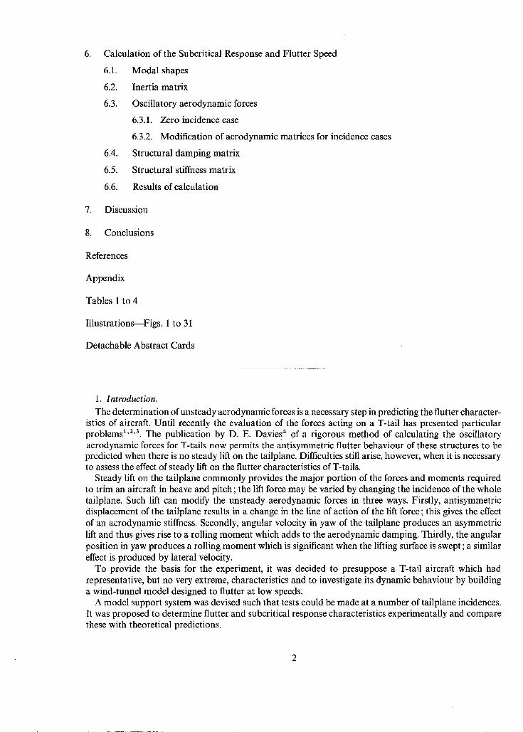
Calculation of the Subcritical Response and Flutter Speed

Modal shapes

Inertia matrix

Oscillatory aerodynamic forces

6.3.1. Zero incidence case

6.3.2. Modification of aerodynamic matrices for incidence cases

6.4. Structural damping matrix

6.5. Structural stiffness matrix

6.6. Results of calculation

7. Discussion

8. Conclusions

References

Appendix

Tables 1 to 4

Illustrations--Figs. 1 to 31

Detachable Abstract Cards

1. Introduction.

The determination of unsteady aerodynamic forces is a necessary step in predicting the flutter character- istics of aircraft. Until recently the evaluation of the forces acting on a T-taft has presented particular problems 1'2'a. The publication by D. E. Davies 4 of a rigorous method of calculating the oscillatory aerodynamic forces for T-tails now permits the antisymmetric flutter behaviour of these structures to be predicted when there is no steady lift on the tailplane. Difficulties still arise, however, when it is necessary to assess the effect of steady lift on the flutter characteristics of T-tails.

Steady lift on the tailplane commonly provides the major portion of the forces and moments required to trim an aircraft in heave and pitch; the lift force may be varied by changing the incidence of the whole tailplane. Such lift can modify the unsteady aerodynamic forces in three ways. Firstly, antisymmetric displacement of the tailplane results in a change in the line of action of the lift force; this gives the effect of an aerodynamic stiffness. Secondly, angular velocity in yaw of the tailplane produces an asymmetric lift and thus gives rise to a rolling moment which adds to the aerodynamic damping. Thirdly, the angular position in yaw produces a rolling moment which is significant when the lifting surface is swept; a similar effect is produced by lateral velocity.

To provide the basis for the experiment, it was decided to presuppose a T-tail aircraft which had representative, but no very extreme, characteristics and to investigate its dynamic behaviour by building a wind-tunnel model designed to flutter at low speeds.

A model support system was devised such that tests could be made at a number of tailplane incidences. It was proposed to determine flutter and subcritical response characteristics experimentally and compare these with theoretical predictions.

2. Apparatus. 2.1. Model.

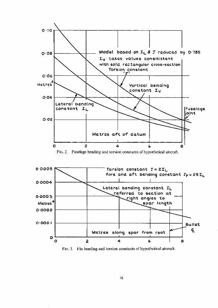
2.1.1. Design. The model represented the rear fuselage and tail unit of the hypothetical aircraft, which was assumed to flutter at a height of 6100 m (20 000 ft) and an E.A.S. of 259 m/s (850 ft/s). The geometry and structural characteristics of this aircraft are shown in Figs. 1-3, and its mass distribution is listed in Table 1. The model was as large as could be accommodated in the R.A.E. 5 ft open jet wind tunnel; the other scaling parameters (Table 2) were chosen to give dynamic similarity to the full-scale aircraft.

The section of the fin and tailplane was RAE 101 with a thickness chord ratio of 6~ per cent. Whilst ttiis section is thinner than those normally chosen for high subsonic speed aircraft, it was felt that finite thickness effects, for which the aerodynamic calculations do not make allowance, would be minimised. Symmetric flutter of T-tails involves tailplane distortion only, and the flutter behaviour is therefore similar to that observed in symmetric flutter of a tailplane-plus-fuselage. Tailplane flexibility can also give rise to other complications in flutter behaviour such as that due to effective dihedral caused by lift and steady g loads t'a. It was therefore decided to make the tailplane of the model rigid by comparison with the remainder of the structure, and in this way limit the scope of the experiment to an investigation of antisymmetric flutter behaviour.

2.1.2. Construction. The requirement for a low flutter speed necessitated the manufacture of a model with low stiffness-to-mass ratio. A diagram of the model geometry, which includes leading dimen- sions, is given in Fig. 4 and the mass distribution is listed in Table 3. The model was assumed to be 'built-in' at a position corresponding to the wing/fuselage intersection of the hypothetical aircraft.

The construction may be seen in Fig. 5. The rear fuselage structure was a light alloy beam providing representative stiffness in horizontal and vertical bending and in torsion. Ribs attached to this beam carried the extra masses which were necessary to achieve the design mass and inertia distribution. The ribs also carried annular glass fibre segments which formed the fuselage profile; the segments were separated from one another by thin polyurethane foam strip. A fitting bolted to the rear end of the fuselage beam carried the fibre glass tail cone, the foam plastic tail cone fairings, the exciter attachment and the fin.

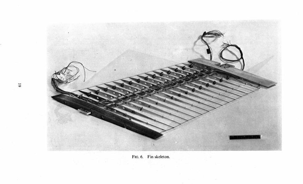
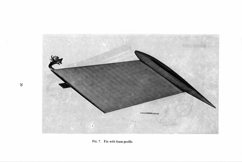
The fin structure (Fig. 6) consisted of a single spar swept back at 40 °. It was machined from one piece of L65 aluminium alloy material, and had an 'I' cross section tapered slightly in both elevations from root to tip. Ribs were glued to the spar, parallel to the fuselage datum and normal to the plane of the fin. These carried concentrated masses ahead of and aft of the spar, to provide the design mass and inertia distribution. The fm profile was achieved by moulding a casing of flexible polyurethane foam--'Flexalkyd' --around the siructural skeleton (Fig. 7). The foam was sufficiently stiff to transfer the aerodynamic loads into the ribs without significant distortion but flexible enough to contribute only very slightly to the flexural and torsional characteristics of the fin.

The tailplane was rigidly attached to the upper end of the fin spar and the joint was faired by a solid spruce bullet. The structure of the tailplane consisted of a laminated spruce main member with balsa leading and trailing edges; the whole was encased by a 0.005 inch skin of glass fibre reinforced plastic.

The completed model is illustrated in Fig. 8.

2.1.3. Characteristics. Irwin and Guyett 5 reported considerable variation in the flutter speed of a model wing because of variations in its structural stiffness. They ascribed these variations to changes in the structural properties of the plastic foam covering of the model resulting from changes in ambient conditions. Because the ribs lay in the plane of the wing, and the distance between them was small, high shearing stresses were set up in the foam when the wing deformed in torsion. In order to avoid difficulties of this sort the fin ribs of the T-tail model were designed to lie in the planes parallel to that of the tailplane.

Static tests were made to check that the design characteristics had been realised. These showed that the foam made comparatively little contribution to the fin stiffness, but that the stiffness of the fin skeleton was appreciably higher than the stiffness of the spar alone. A further static test confirmed that the cause of this difference was associated with the alignment of the fin ribs. The ribs are designed to transfer shear force and bending moment from the leading and trailing edges into the spar. However, their alignment

is such that they contribute greatly to the section modules and torsion constant of the spar; in this way they increase the stiffness of the fin.

Calculations based on measured values of fin stiffness and assumed modes of vibration indicated that flutter would occur at a wind speed of 30.2 m/s (99 ft/s), when the tailplane was at zero incidence.

2.2. Model Support System.

The rigging arrangements are shown in Fig. 8. A glass fibre nose fairing covered the machined steel saddle which attached the model to the supporting rig. The saddle was carried on an axle which permitted the angle of incidence of the model to be varied. This axle was mounted in a tubular steel framework based on steel girders which were bolted to the floor of the wind tunnel. The incidence of the model could be changed either manually by the adjustment of a turnbuckle or electrically by the operation of a screw jack. During test runs the tailplane incidence was measured optically.

2.3. Excitation.

The model was vibrated antisymmetrically by an electro-magnetic exciter comprising a coil moving between the poles of a permanent magnet (Fig. 9). The coil was wound over a light glass fibre former and suspended from a parallel linkage arranged so that the length of travel was +_ 1-9 cm (_+ 0.75 inch). The fixed end of the linkage was attached to a plate which was anchored by a supporting framework. The force provided by the coil was transmitted through a light rod and two universal joints to the tip of the tail cone. There was thus a small increase in stiffness and inertia of the model system over the scaled stiffness of the hypothetical aircraft.

The current for driving the coil was obtained by amplifying the sinusoidal output of the decade oscillator in the ELVIRA equipment 6 (Fig. 10). Amplitude and phase of the exciter current were determined by measuring the voltage drop across a resistance in series with the exciter coil. The amplitude was adjusted by altering either the drive of the oscillator or the gain of the power amplifier so that there was a fixed peak force input to the model. A phase change occurred between the force input to the coil and the oscillator signal because of the amplifier characteristics and the back emf in the coil; this was compensated for in the recording equipment.

2.4. Instrumentation.

The response of the model in the wind tunnel was sensed by strain gauges glued to the fin spar; these were arranged in a series of four-arm bridges sensitive primarily to bending moment or shear force. Four bridges--two bending, two shear--were attached at the root station, and one bending bridge was attached at mid span. The wiring arrangement and some of the gauges can be seen in Fig. 6. The output of each bridge was fed directly to the ELVIRA equipment. Transducer signals were displayed as voltage measure- ments of the response in phase and in quadrature with the exciting force. The output was typed and punched on paper tape; it was also fed to a Bryans X-Y Plotter for direct drawing of the vector response plots.

The response of the model in still air tests was measured by a Wayne Kerr vibration meter. For these tests copper foil discs were temporarily attached to the model in the positions shown in Fig. 11. Thirty probes were connected to a mechanical switch; the output of each was taken in turn to the Wayne Kerr vibration meter and led thence to the ELVIRA equipment.

3. Flutter Tests.

The critical flutter speed was found by increasing the wind speed in small steps, and at each step seeing how rapidly the vibration caused by a slight perturbation of the model died away. Initially a transient disturbance was applied to the model, but at speeds approaching the flutter speed the tunnel turbulence provided adequate excitation. The flutter frequency was determined from a display of the strain gauge outputs on an oscilloscope.

Flutter speed and frequency remained virtually constant during the zero incidence tests at 30.2 m/s (99 ft/s) and 2.7 Hz. The tests were conducted with and without the exciter system connected, but no

significant change in flutter behaviour was observed. For tests with incidence the wind tunnel was set to run just below the critical flutter speed, and the

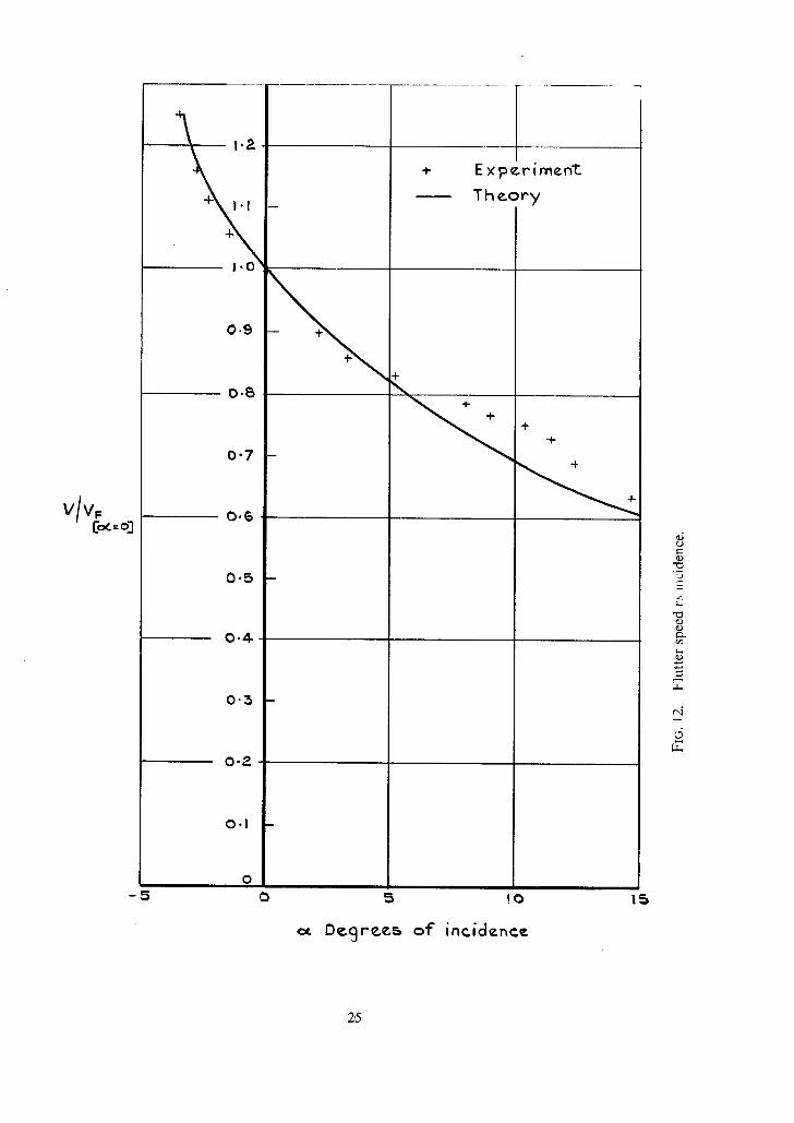
tailplane adjusted to the required angle of incidence. The wind speed was then increased in small steps; the airflow was turbulent enough to excite flutter when the critical speed was reached. Measurements were made at a series of incidences between - 3.5 ° and + 14.6 ° and the results are shown in Fig. 12.

4. Response Measurements in the Wind Tunnel.

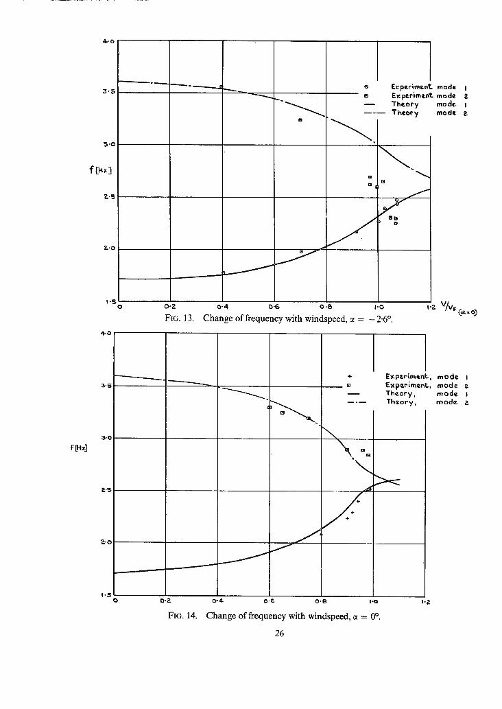
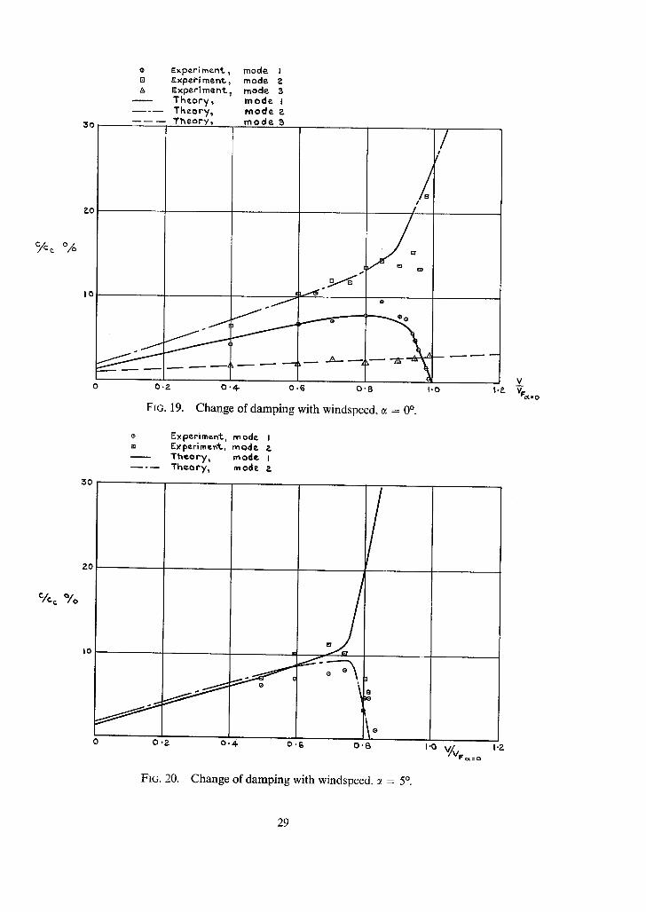
Response characteristics were measured over a range of wind speeds up to the critical flutter speed at tailplane incidence settings of -2 .6 °, 0 °, 5 °, 10 ° and 15 °. The model was sinusoidally excited at a fixed peak force over a band of frequencies about each resonance, and the response was obtained from the strain gauges mounted on the fin spar. The Elvira equipment was used to measure the response and to provide a series of vector plots from which the resonance frequencies and dampings in the first three modes were obtained. The results for the two modes principally involved are shown in Figs. 13-27. The response in the third mode is illustrated in Fig. 19.

5. Response Measurements in Still Air. 5.1. Test Procedure.

The tests procedure was similar to that used for measuring the response in the wind tunnel, with the difference that displacements were measured by the Wayne Kerr vibration meter at the stations shown in Fig. 11. In addition to these, two probes were mounted vertically at the base of the fin to see if there was any significant fuselage rolling motion. The rolling motion of the tailplane was obtained by probes measuring vertical displacements at the tips; these values were consistent with those deduced from displacements of points at the top of the fin.

5.2. Determination of Resonance Frequencies and Modal Shapes. In each mode the resonance frequencies and amplitudes and hence the normal mode shape was inferred

from the vector response plotsS: The assumption of orthogonality in modes 1, 2 and 3 is thought to be justified by the cross-inertia check (see Table 4).

The derivation of inertia, damping and stiffness matrices from these measurements is described below.

6. Calculation of the Subcritical Response and Flutter Speed. The matrices in the equations of motion of the system were calculated from the response measurements

in still air and the model characteristics. The degrees of freedom chosen and the preparation of the co- efficients are described below.

6.1. Modal Shapes.

The first three modes of the model were taken as the degrees of freedom of the system. The measured shapes of these modes are shown in Figs. 28-30.

6.2. Inertia Matrix.

The inertia matrix was derived from the mass distribution of the model (Table 3) and the measured modes in still air (Figs. 28-30). Vertical displacements of fin and fuselage were small and their contribution was neglected. The normalised matrix (Table 4) showed a value of about 5 per cent for the cross terms between modes 2 and 3.

6.3. Oscillatory Aerodynamic Forces.

6.3.1. Zero incidence case. The method of D. E. Davies 4 was used for calculating the generalised aerodynamic coefficients for the T-tail. This method uses a Mercury Autocode programme RAE 264A which requires as input the displacement and slopes at selected points on the fin and tailplane. In the

present work this information was derived from the modes measured in still air. It was necessary to include in the input an assumed value of frequency parameter; this was derived from the preliminary flutter tests. No allowance was made in the calculations for any fin-fuselage interference effects.

6.3.2. Modification of aerodynamic matrices for incidence cases. When the tailplane is at incidence it experiences a normal force which produces aerodynamic stiffness and damping terms 7 in addition to those calculated for the zero lift condition. Furthermore the effective sweepback of the fin is increased although the presence of fuselage and tailplane may tend to re-align the flow as shown in Fig. 31a. The method used in Ref. 4 may then be applied to the calculation of the air forces. In order to modify these by introducing tailplane lift effects the following assumptions are made:

(1) The symmetrical part of the lift is constant in magnitude during an oscillation and acts at a fixed point on the tailplane centreline, as shown in Fig. 31b. When the tailplane is displaced the line of action of the lift changes giving an aerodynamic stiffness effect.

(2) The antisymmetrical part of the lift, which occurs when the tailplane has angular velocity in yaw, can be represented by a rolling moment about the tailplane centreline, as shown in Fig. 31c. This moment produces an aerodynamic damping.

(3) Of the sideslip effects which occur when the tailplane is displaced in yaw or moving laterally the rolling moment is the most important. The steady load part of this effect is not included in Ref. 4, and modifications are made here, based on R.Ae.S. data sheets.

The problem of calculating the aerodynamic air forces is thus reduced to deriving the aerodynamic matrices for zero incidence and superimposing matrices representing the effect of lift. With these assump- tions the aerodynamic stiffness and damping matrices for the model at incidence can be calculated. The magnitude of the lift is derived from lift-curve slope data for flat plates a, the effect of tailplane thickness and bullet being neglected as in the zero incidence case ; these values were checked by direct measurement of tail loads on the model. Details of the derivation of the lift effects are given in the Appendix.

6.4. Structural Damping Matrix. The diagonal terms in the structural damping matrix were derived from response measurements in

still air. The assumption was made that the cross-damping terms were zero. Previous work s has suggested that the calculations are unlikely to be influenced significantly by small structural cross-damping terms.

6.5. Structural Stiffness Matrix. The direct terms of the structural stiffness matrix were determined from the direct terms of the inertia

matrix and the modal frequencie s; cross-stiffness terms were made zero.

6.6. Results of Calculation. The equations of motion of the system were solved by the computer programme RAE 272, which

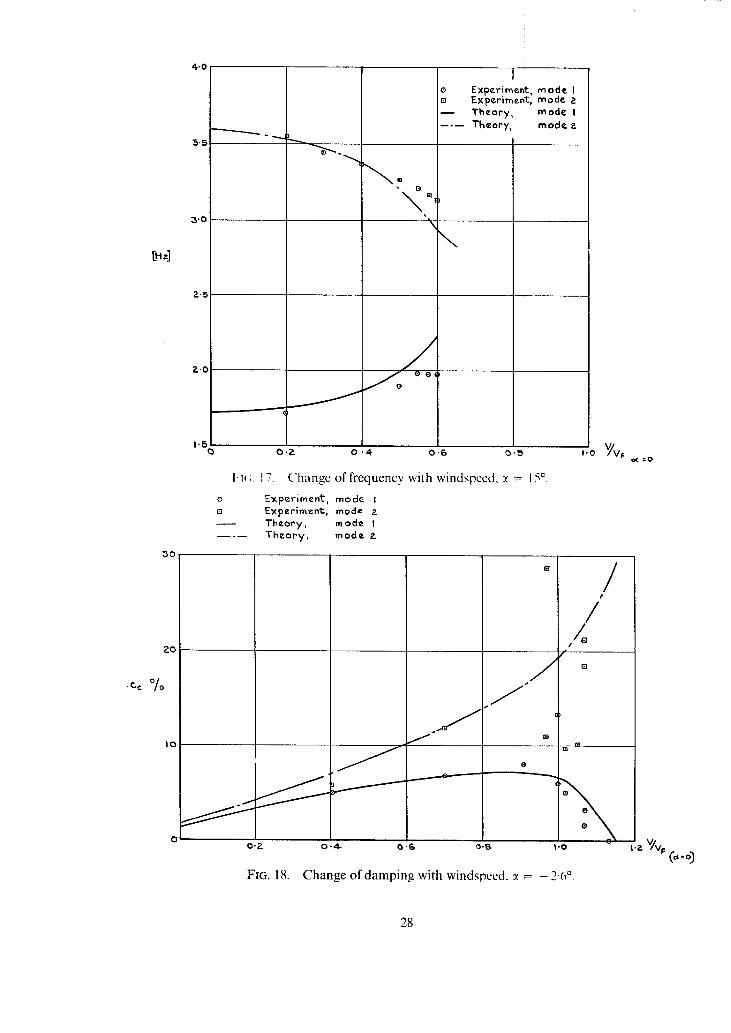
employs Mfiller's method for extracting complex roots. At a given value of windspeed the programme determines for each mode a complex number whose imaginary part is proportional to the circular fre- quency and whose real part is proportional to the decay rate. Figs. 13-17 show the change of frequency with windspeed for two of the three modes in the calculation and Figs. 18-22 show the corresponding dampings. Fig. 19 also includes the response in the third mode.

When the subcritical response and flutter characteristics are calculated using aerodynamic matrices modified to include lift effects, the following changes are predicted :

(1) Flutter speed Vr decreases as incidence increases. At an angle of attack of 15 ° flutter is estimated to occur at about two thirds of the calculated critical speed at 0 ° (Fig. 12).

(2) At zero or negative incidence damping falls to zero in the first mode (Figs. 18 and 19); at angles of incidence greater than 5 ° the damping falls to zero in the second mode (Figs. 20, 21 and 22).

(3) The onset of flutter is sudden in the 5 ° incidence region (Fig. 20).

7. Discussion. The main purpose of the investigation was to show that flutter and sub-critical response could be

predicted using aerodynamic forces computed by the methods given in Ref. 4 with modifications to take account of steady tailplane lift. Before considering the degree of success achieved it is necessary to mention possible sources of experimental error. Those may be listed under three headings: (i) errors in mode measurement, (ii) difficulties of analysis of wind-tunnel responses in the presence of unsteadiness in the tunnel flow and (iii) difficulties in extracting modal information from the responses of two modes having nearly coincident frequencies. The errors arising under (i) affect the validity of the calculated aeroelastic behaviour, whereas the error under (ii) and (iii) made it difficult in some conditions to obtain experimental data of acceptable accuracy.

It was found from the calculations, and confirmed experimentally, that the flutter behaviour of the model depended essentially on modes 1 and 2, and in the presentation of results the frequency and damping of mode 3 has been omitted, except in Fig. 19 which illustrates that the damping increases linearly with wind speed throughout the test range.

Examining first the change in flutter speed VF with incidence (Fig. 12) it is seen that flutter speed drops as tailplane incidence increases. Agreement is good when ~ is small; agreement is not so close when tailplane incidence lies between 7.5 ° and 12.5 °, although even here calculated flutter speeds are within 10 per cent of the measured values.

Figs. 13 to 17 show the variation of modal frequency with windspeed over a range of incidence for modes 1 and 2, and Figs. 18 to'22 the corresponding damping variation. The frequency curves (Figs. 13 to 17) show broad agreement between theory and experiment, with some discrepancies at negative incidence (Fig. 13), and they illustrate the degree of scatter that can arise in analysis of response data when modal frequencies are close together. The damping curves (Figs. 18 to 22) generally show good agreement between theory and experiment at speeds well below the critical flutter speed, but discrepancies arise as the critical speed is approached. In this region, scatter of the experimental values of damping and frequency is increased.

An important result in Figs. 18 to 22 is that whereas at ~ = -2.6 ° or ~ = 0 ° the calculations show that it is mode 1 which has zero damping at the critical flutter speed, at ~ = 5 ° and above, mode 2 becomes zero damped. The experimental results confirm this behaviour at ~ = -2.6, 0 ° and 15 ° but at c~ = 5 ° and 10 ° (Figs. 20 and 21) the measured damping on both modes appear to tend to zero as the flutter speed is approached. This is the major discrepancy between experiment and theory, and it may be signifi. cant that the largest discrepancies in flutter speed also occurs in this same region of incidence (~ = 10°).

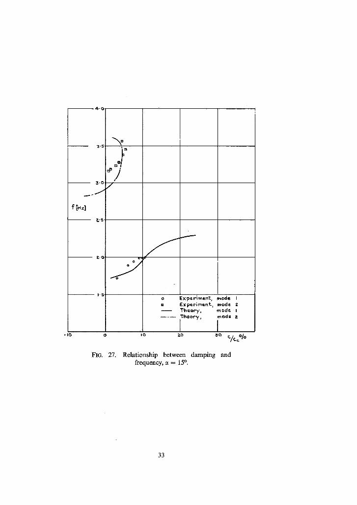
Figs. 23 to 27 show the relationship between damping and frequency. These plots show clearly the change of the zero damping condition from the low to the high frequency branch as incidence is increased. The discrepancies in the changeover region are again apparent; the absence of high damping values in the experimental data and the presence of low damping values in both measured modes are not readily accounted for.

8. Conclusions.

The tests have shown that the flutter behaviour of a low-speed T-tail wind-tunnel model can be success- fully predicted by calculations based on the theoretical work of D. E. Davies 4. By applying a simple modification, calculations can be extended to take into account the effects of steady tailplane lift.

Increase of incidence resulted In decrease of flutter speed; there was a reduction in flutter speed of 50 per cent in the range of incidence ~ = - 3.5 ° to ~ = 14.6 °. At incidences of 10 ° or more the motion in flutter was predominantly fin torsion in contrast to the fin bending seen in flutter at zero incidence.

The single-point excitation system adopted for the tests permitted the extraction of a set of modes which were effectively orthogonal for the purposes of calculation.

It was found that the calculated subcritical response agreed well with values obtained experimentally at speeds up to 90 per cent of the flutter speed, and that the actual flutter speeds were predicted with a lair degree of accuracy. At speeds immediately below the critical speed the response of the more highly damped mode proved difficult to extract because of the merging of the circle plots. In addition turbulence in the tunnel caused a good deal of interference so that in this application the vector response technique for deducing frequency and damping was not altogether satisfactory.

The 'backbone' type of model adopted for the experiment proved well suited for low-speed wind-tunnel

testing. The design was such that the polyurethane foam profile of the fin was very lightly stressed and so contributed little to its structural characteristics; there was no discernible change caused by variations in ambient conditions.

No. Author(s) 1 J.C.A. Baldock ..

2 S.A. Clevenson and .. S. A. Leadbetter

3 N.S. Land and A. G. Fox ..

4 D.E. Davies . . . . . .

5 C.A.K. Irwin and P. R. Guyett

6 W.D.T. Hicks . . . .

7 P.R. Guyett . . . . . .

8 J. de Young and C. W. Harper

REFERENCES

Title, etc. The determination of the flutter speed of a T-tail unit by calculat-

ions, model tests and flight flutter tests. AGARD Report 221 (1958).

Measurement of aerodynamic forces and moments at subsonic speeds on a simplified T-tail oscillating in yaw about the fin mid-chord.

NACA TN 4402 (1958).

An experimental investigation of the effects of Mach No., stabilizer dihedral, and fin torsional stiffness on the transonic flutter characteristics of a tee-tail.

NASA TN D-924 (1961).

Generalised aerodynamic forces on a T-tail oscillating harmoni- cally in subsonic flow.

A.R.C.R. & M. 3422 (1964).

The subcritical response and flutter of a swept-wing model. A.R.C.R. & M. 3497 (1965).

A control and measurement system for aeroelastic model tests. A.R.C.C.P. 1045 (1968).

AGARD Manual of aeroelasticity. Part 2--Aerodynamics derivatives. Chapter 11--Empirical values of derivatives.

Theoretical symmetric span loading at subsonic speeds for wings having arbitrary planform.

NACA Report No. 921 (1950).

APPENDIX

The method given in Ref. 4 for calculating air forces on an oscillating T-tail applies only when the tailplane is at zero incidence, and when there is parallel flow over the fin surface. In the present work the whole model when at incidence has, in addition to the lift developed on the tailplane, a complicated flow pattern over the fin surface. In order to allow for these effects the following assumptions are made :

(1) The air forces on the fin are not altered substantially when the flow has a small component normal to the tailplane; the effect is assumed to be that of a flow parallel to the tailplane as shown in Fig. 3 la.

(2) The air forces on the tailplane are those developed at zero incidence together with those resulting from the action of the lilt force. These lift-induced air forces are derived in the following way :

The lift force on a tailplane at incidence is :

+ S

L= f ½p V 2 Clc dy - - s

where L = lift force

p = air density

V = air velocity

Cz = local lift coefficient

c = local chord

y = spanwise co-ordinate (positive to starboard)

s = semi-span

Ref. 8 gives the value of Ct as a function o f y for a variety of planforms: lift forces calculated for the model tailplane were confirmed by direct measurements of load.

The lift is assumed to be normal to the tailplane and constant in magnitude during small oscillations of the model. The tailplane has rigid body freedoms in roll, yaw and lateral displacement. Work is done by the lift force in the following circumstances :

(i) When the tailplane is displaced in roll through a small angle 0 the lift force does work if lateral displacement r/occurs. The generalised rhs force* developed in mode q' due to displacement in mode q (sign convention in Figs. 31b and c) is

at/ 00 L ~ ~qq

(ii) When the tailplane has an angular velocity in yaw, the change in Velocity over the span produces a rolling moment (Fig. 3 lc). For an angular velocity in yaw ~ the effective windspeed over a chordwise strip distant y from the centreline is

Hence

V+$y

*i.e. disturbing force on the model.

10

(. = jo vE v+6yj Ctcdy

to first order in 4~. The term in q~ does not contribute to the total lift, as it disappears on integration over the whole span, but it gives a moment

M = f p Vdpy2Ctcdy = M ~ .

Work is thus done when the tailplane is rolled and the generalised rhs force in mode q' due to displacement in mode q is in this case :

Oq'

where ~q 0 = q~.

(iii) The foregoing derivation of lift and rolling moment is based on an airflow which is symmetrical with respect to the tailplane planform. This assumption is not valid when the tailplane is displaced in yaw, or when it has a lateral velocity. The rotation of the tailplane through a small angle q~ produces a sideslip effect due to change in both sweepback and aspect ratio relative to the direction of flow. An effective sideslip angle - O/V is produced when a lateral velocity 0 takes place. The effect of sideslip is to displace the centre of pressure in a spanwise direction. The displacement for unit angle of sideslip is obtained from R.Ae.S. Data Sheet 06.01.04, which gives the conversion factor for a variety of planforms. In the actual model the displacement of centre of pressure is found to be

d = 0"6sfl

where fl is the angle of sideslip and s the semi-span. So the rolling moment for yaw displacement ~b is

and the rolling moment for lateral velocity 0 is

-0 -6 Ls

-0 .6 Ls O/V .

The generalised rhs forces in mode q' due to sideslip effects are thus

resulting from yaw displacement, and

- O-fl-O o'6 Ls ~q

O0 0"6Ls Or I . Oq' V Oq q

resulting from lateral velocity. The forces derived in (i), (ii) and (iii) above are added to the zero incidence terms. Simple harmonic

motion with circular frequency co is assumed, so 0 is replaced by io~q in the equation of motion.

11

Station

metres aft of fuselage fixing point

0"60 1.80 4'20 5.40 6.60

Fuselage 8-10 9-15

[0.05 11.10

1.55

metres above fuselage centreline

f 0.92 1.84

Fin 2.75 3-66 4.57 5.25

metres outboard of bullet centreline

r0

0.24 0.72 1.27 1.68

Half-tailplane 2.16 2.59 3.12 3.65 4.08 4.56

TABLE 1

Mass Distribution of Hypothetical Aircraft.

Lumped Radius of mass gyration about (kg) centroid (m)

608 1.16 1134 1.15 1324 1"15 1288 1.15 987 1.15

1082 1-15 721 1.04 457 0.84 197 0.71 79 0-67

15 0-231 of chord 12 ,, 12 ,, 13 ,, 12 ,, 16 ,,

7 ,, 9 ,, 6 7, 6 6 ,, 6 ,, 6 ,, 4 ,, 4 1

Other information

Region of bullet and joint construction

12

TABLE 2

Scaling Factors

Property Model/aircraft Length 0-0833 Mass 0.00108 Stiffness 0.00000803 Frequency 1.03 Deflection (gravity) 0.935 Strain (gravity) 11.2 Deflection/load 865 Strain/load 10400

TABLE 3

Mass Distribution of Model.

Fuselage

Section

1 2 3 4 5 6 7 8 9

10

Distance from fixing point

(m)

0"05 0-15 0"35 0"45 0"55 0"675 0"76 0"84 0"925 0"96

Mass (kg)

0.66 1-23 1-44 1.40 1.07 1.18 0.78 0"50 0"22 0.09

Moment of inertia in roll kg m 2

0-0062 0-0114 0.0135 0.0130 0"0096 0.0110 0'0054 0.0026 0.0008 0.0004

Moment of inertia in yaw kg m 2

0.0034 0.0060 0.0072 0.0068 0.0050 0.0084 0.0030 0.0012 0.0004 0.0001

Fin

Distance above fuselage Cz Mass Moment of inertia in yaw Section m kg kg m 2

0.04 0-09 0-14 0.19 0.24 0.29 0.35 0.40

0.050 0.140 0"050 0-150 0.050 0.150 0.054 0.204

0.0008 0"0030 0.0008 0.0030 0.0008 0.0030 0.0012 0.0042

Tailplane and bullet cg 0.0919 m aft of spar top. Mass = 1.28 k g Moment of inertia in roll = 0.0495 kg m2( Moment of inertia in yaw = 0.0604 k# mZJ about cg

13

TABLE 4

Normalised Inertia Matrix.

Mode

1 0"031

-0"013

0"031 1 0"050

-0"013 0"050 1

14

B'66

L imi¢ o f _ "Fuselage

p r o f i le

I ~ F i x i n 9 da tum I win9 f u s e l a g e I i n t e r s e c t i o n

L im i t o f f u s e l a g e p ro f i l e

• / ~ 55~ II 9 - 6 0

1 ~ 1 - 9 o ~ ; ~ 3 " 3 9 1 . 4 5 2 " 5 8 l

k e ~ ~ - - 1 - - ~ 10-06

I I

. / / j / ------------L_Ji / i/

I I

; / V~sov ~ J / 3"66

rJ

; I !

1 I I I I

5-49

J I

l_

Dimensions in m e t r e s

00.6 0

FIG. 1. Line diagram of hypothetical aircraft.

t _1

I

0 ' I 0

0 ' 0 8

0 "06

Metres 4

0"04

0 ' 0 2

0

Model based on I u @ J" reduced by

I V tokes values consisistcnt wlth solid rectangular cross-section

T°rsi°n, orC,°n st°n%

Vcr~cical b¢ ,nd in 9 ,= I ~constont I v

Latcro| bcndinc. consCant 3; L

FIG. 2.

M ~ t r c s a ~ t o~ dcL tum I

I I 2 4. /=

Fuselage bending and torsion constants of hypothetical aircraft. 8

0"785

F u s ¢ l o q ¢ i o i n t

0 " 0 0 0 5

0"0006

0 . 0 0 0 : 5

M~tr~s 4

O.OOOR

0"000 a

0 0

. • • r e r a l bcndin 9 constant IL fcrred to section ~±

• ~ ~ g h t angles to - -

Torsion constant ~T= ~ I L form and of± bcndin 9 cons%ant

Metres Qlon 9 s p o r from coot I !

2 4 6

TF= 2 5 I k

Bullet

8

FIG. 3. Fin bending and torsion constants of hypothetical aircraft.

16

/ \ / \

\ \

\ \

/ \ ! \

I I I I L I

!

\ / \ ! \ /

/ /

/

Nozzle of R.'A.E 5f't open ,j£'k

wind tunnel.

m E .~

, , r a

0 . 8 3 8 m

J Wind tunne l f loor .

FIG. 4. G e o m e t r y o f m o d e l a n d rig.

+

. . . . . . . . j -+" ;,~,+, ~ • +"~. + - , I " ° - ? + ')~r+

• ~ ..++ ~ ,

,,+ J \+,

L ~

FIG. 5. M o d e l w i t h f u s e l a g e p r o f i l e r e m o v e d .

' ' - 7

FIG. 6. Fin skeleton.

. . • •

I ' O

/

• ~ , ~ . . . . ~ .

FIG. 7. Fin with foam profile.

t,9

r 1¢5. 8. Model and supporting rig in wind-tunnel.

jb

• . 3

i t

j,

FIG. 9. Electromagnetic exciter.

22

FIG. 10. Resonance testing of the flutter model.

bO

Gcate 1 : 6 - b b ' /

Fusetag~ f'ixing point

(9 ® G ®

FIG. 11.. Lateral displacement measuring positions on model.

v/vF [0¢-- o]

- 5

• 1,2

-F l . I - -

0-9

0.8

0.7

0,6

0-5

0-#

0-2

0

o

o.I

E x p e . r i m ~ n ~

Th~_ory

-l"

-I-

5 la 15

(x D~.cjre.e~ o f incicl~ne.~.

, j

z

b.

b.

25

4-.o

~-5

f[H~]

?-'5

?.-O

1 .5 0

4,0

3 . 5

~-0

P..5

~ '0

t . 5

e Exp~r im~n t m o d e I m E x p e r i m ¢ ~ mode ?.

T h e o r y m o d e I _ _ _ m T h e o r y m o d e z

B

O.Z 0 "4 0"6 0 .B I ' 0

FIG. 13. Change of frequency with windspeed, ~ = - 2-6 °. I.z v/vF C..o )

l J

+ E x p e r i m e n m o d e I o E x p e r l m e r m o d e z

T h e o r y . m o d e I T h e o r y , mode . ?.

a \ Q "x,,

J ,p

O o - z 0 . 4 o . ~ o . 8 ~ .o

FIG. 14. Change of frequency with windspeed, ~ = 0 °.

26

I-Z

3 , 5

ft.=]

7..0

1.5

f

\ \

f

E x p e r i m e n t , E x p e r i m e ~ T h e o r y , T h e o r y ,

×

o ,2 o . ~ o .G o .B

m o d e I m o d e 2 m ode.. m m o d e z

,.o v/v~. :o0

f[Hq

4 ° 0

~5.5

7PO

?..'5

~...0

1.5 0

FIo. 15. Change of frequency with windspeed, ~ = 5 6.

J

t a

\

J

e Expe.rimen~., m o d e I

I~ E x p e r i m e n t , m~ ~. l'h¢ory > m+ I Theory m< z

\o Eg

J G

0 - 2 0-4- 0 " ~ 0.~, 1"0 V/vF~.o FIo. 16. Change of frequency with windspeed, ~ = 10 °.

27

4 ,0

~5.5

:3,0

F_,O

1"5

/ I

"~o \

\

I Exp¢r ime~t , m o d e I Exper iment , mode 2 T h e o r y , m o d e I Theory , m o d e

I

0 ' 2 0 . 4 0 "6 O'B

tl~;. 17. ( ' h a n g e of f requency with windspeed . ~ = 15 °.

Experiment, mocle I Experlm~nt, mode 2

The.or,/ , mode I T h e o r y , m o d e &

I '0 V//V F eK=o

gO

/C c °/o

IO

. / /

. / /

O . Z o -~- 0 . ~ o.e ,

/ F

/ /

1.O

FIG. ] 8. C h a n g e of d a m p i n g with windspecd . ~ = - 2-6 °

28

e Experiment ~ mode I [] Experiment, m o d e A Experiment I mode,

Theory~ mode I Theory~ mode z

- - - - - - Theory~ m o d e ~,

gO

I0 . J

4 ~ j c

. ~ ? ~ ~ - - - - ~ ~ ~ "L

FIG. 19.

/ / /

O

0 ,,~ 0,6 O'B

Change of damping with windspeed, ~ = 0 °.

1 , 0 t.P-..

30

Expmrimcnt, m o d ~ I Expcrimen%, m o d e T h e o r y ~ m o d e I T h e o r y ~ mod&

ZO

|0

J J

/

O

0 0 , ~ 0 . ~ 0 , ~ O ' B

/

F16.20. Change of damping with windspeed, :~ = 5 °.

I'(~ V//VF = = ~ I'7-

29

80

| 0

"SO

0 0 "0 "~ O . B

J

m

0 O m

tg \° m

o.~- 0 .6

FIG. 21. Change of damping with windspeed, ~ = 10 °.

Experimcn'1:, mode u Ey, per lmen~; , modGt g

l "heol 'y , mode I THeary , m odz e.

1,0 V/V I'Z F~ . : 0

30

80

I0

®

---, \

I I Exper iment • r~ode ~xpe r imen t ~ m o d e Theory/, m o d e Theory , m o d e

0 ~ ' ~ 0 "4- 0 - ~ O'B I '0 YVF ,~.=o 1.2

FIG. 22. Change of damping with windspeed, ~ = 15 °.

30

25-~

~[,z]

-I0

%

o r~

W

Q

Z'O

I -5

El Q

Expe.rim¢nt, mode I Exp¢riment, mode 2 The.ory, mode I

m " m ~h¢Ory, mode ?.

0 I0 P.O Z~O C/C¢ " °/o

FIG. 23. Relat ionship between damping and frequency, ~ = - 2.6 °.

4 .0

3 .0

?.-5

?-.0

| 'S

\

e Exper lnnent, mode I m E~cperiment, mode ?_

Thc.ory , mod¢ I m -- m T h e o r y , m o d e ?_

o ,o zo ~o %~ 7o

FIG. 24. Relat ionship between damping and .frequency, ~ = 0 °.

4-.O

b~

~.5

.~.0

f[H:]

®

z oo

\

\ )

/ J

°% ®

-~0

¢ Exper lm~nt , ~od~ I Exper iment , mod¢ P. T h e o r y , mode I Theo ry , mod~ 2

I

l-l•. 25. Relat ionship between damping and frequency, ~ = 5 °.

f[.,]

-IO

:3"5

~-0

J

Z'5

Z.O

1.5

\°° /

®

0

o

® ®

jY o Exp~rlm~nt.-, mode. I

Experiment, mode Theory, ~ocl~ 1 Theory, mode- 2

I-IG. 26. Relat ionship between damping and frequency, c~ = 10 °.

-,j,~

3 " 0

f [H-]

?.'5

| .~

, 1 0 0

/

f

® E × p e r i m e n t ~ node I = E x p e r i m ~ n t ~ mode Z

T h e o r y , m o d e I - - - - - " t h e o r y / mode Z

I0 2.0

FIG. 27. Relationship between damping and frequency, ~ = 15 °.

33

FIG. 28. Lateral displacements of fuselage and fin in still air--Mode 1.

\ FIG. 29.

\ FIG. 30.

Lateral displacements of fuselage and fin in still air--Mode 2.

Lateral displacements of fuselage and fin in still air---Mode 3.

34

- / V

Zero incldenc¢ case :

No fo rces on to i lp lane

or f in when model is in neutral position

V Fo< vz o~

V

Model at incidence Veloci ty over f in surface assumed to be parallel to bullet

(a) Schematic representation of assumed incidence effect. (View from port).

Lilac L ~

Positive i • ..--..- roll ~ ...~.--."

component in direcf~ion of" ~l = L e Displaced

.- .. -- -- positi on ~" "~ Normal

position

/~,-'K ' , ,~) )

(b) Change of direction of lift force due to roll. (View from front).

t ~ Wind i I

Decrease o¢ / e f fect ive . / ~ " windspeed ~ ~ . - - -y

a n . . . ' t f , , , ' l y4 ,nc,-=o,, of,weepboek I f"

"','°°~ ~°"° ° ° " iN L . . . - - ~ . - - " '

Positive yaw 1

~ Wind

y~ Increase o f e f f ec t i ve windspeed and l i f t

_ Decrease o-F sweepbock~ ~ i n c r e a s e o¢ effect ive

. ~ - - ~ I,~ aspect rat io and Ir f t

I ~ ' ~ - ~ J ~--Oisplaced osl t ion ' ~ ~ 1 - ' P

~ . J ~ Normal position t t

(c) Rolling moment effects produced by yawing. (View from above). FIG. 31 a to c.

Printed in Wales for Her Majesty's Stationery Office by Aliens Printers (Wales) Limited

Dd. 501372 K.5

35

R. & M. No. 3652

~'3 Crown copvri~,ht t971

Published by HER MAJESTY'S STATIONERY OFFICE

To be purchased from

49 High Holh¢);n. London WC1V 6HB 13a Castle Street, Edinburgh EH2 3AR 109 St Mary Street, Cardiff CF 1 1JW

Brazennose Street, Manchester M60 8AS 50 Fairfax Street. Bristol BS1 3DE

258 Broad Street. Birmingham BI 2HE 80 Chichester Street, Belfast BT1 4JY

or through booksellers

R. & M. Noo 3652

SBN 11 470372 8