The Effect of Rice Price Changes on the Income

The Effect of Rice Price Changes on the Income Distribution of Household Groups in Indonesia (A Non-Parametric

Analysis)

Radi Negara

820911598130

DEC-80433

MSc Thesis Development Economics

August 2010

i

The Effect of Rice Price Changes on the Income Distribution of Household Groups in Indonesia (A Non-Parametric Analysis)

Radi Negara1

MSc Thesis Development Economics

Supervisor: Dr. Kees Burger Associate Professor Development Economics Group Wageningen University The Netherlands Email: [email protected]

1 [email protected]

ii

iii

Abstract

One issue that raises public debate in Indonesia every year is about the price of rice. There is a polemic whether the price of rice should be lower or higher. The dilemma is about protecting rice farmer or rice consumer. Applying non-parametric analysis on Indonesian Family Life Survey 3 data, this study tries to observe the effect of rice price changes on the income distribution of Indonesian households. However there is some vagueness in imputation method for this survey. Other problem concerns the unclear criteria of rice farmer which cause overvalued or undervalued of rice production value estimation. The result clearly gives the detail of variation, which shows us the impact of any changes or policy is not linear and not equal even for the same type of household. Regarding to the impact on total welfare, rice price support does not favour to the poor, neither rice farmers nor consumers. Hence there will be further question on whether current rice price policy which discriminates price for farmers and consumers is effective or efficient.

iv

Table of Contents

Abstract iii

List of Table v

List of Figure v

1. Introduction 1

1.1. Background 1

1.2. Research Question 5

1.3 Methodology 5

1.3.1 Theoretical background 5

1.3.2 Estimation method 7

2. Data 9

2.1 Sample structure 9

2.2 Data Summary 11

3. Results 14

3.1 Income Distribution 14

3.2 Rice Budget Share 15

3.3 Net Benefit Ratio 18

4. Conclusion 24

References 25

Appendix A Program Code (figure 3.2) 28

Appendix B

Living standard and rice consumption (wrice), Indonesia 2000, by provinces 29

Appendix C

Other staple food share averaged by log pce, Indonesia 2000, by provinces 33

Appendix D

Net benefit ratio averaged by log pce, Indonesia 2000, by provinces 37

v

List of Table

Table 1.1 Indonesia rice production and consumption (million tons) 1

Table 1.2 Shares of urban and rural households by farming status 3

Table 2.1 Samples on IFLS 3 10

Table 2.2 Average of per capita expenditure (pce), rice revenue, rice consumption

and budget share of rice per month 12

Table 3: Percentage of losers and gainers from rice price increase, Indonesia 2000 21

List of Figure

Figure 1.1 Indonesia rice import (thousand tons) 2

Figure 1.2 Indonesia rice price and poverty rate 1996-2009 4

Figure 1.3 The price of milled rice and paddy in Indonesia 1980-2004 7

Figure 3.1 Income density 14

Figure 3.2 Living standard and rice consumption in Indonesia 2000 16

Figure 3.3 Joint distributions of net benefit ratio and log pce, Indonesia 2000 18

Figure 3.4 Rice production value averaged by logpce, Indonesia 2000 19

Figure 3.5 Joint distributions of net benefit ratio and log cultivated farm land size,

Indonesia 2000 19

Figure 3.6 Net benefit ratio averaged by log pce, Indonesia 2000 20

Figure 3.7 Net benefit ratio averaged by log land size, Indonesia 2000 21

Figure 3.8 Proportion of households producing rice, Indonesia 2000 22

Radi Negara 2010

1 | R i c e P r i c e a n d I n c o m e D i s t r i b u t i o n

1. Introduction

1.1. Background

Rice in Indonesia is a blessing and suffering all at once. Rice is a main staple food that is consumed by the majority of Indonesians, while its production has strong effects on the welfare of Indonesian households. Rice has become one of the fundamental issues in Indonesia’s agriculture due to its strong relation with poverty. One issue that always raises public debate every year is the price of rice. The dilemma appears whenever the price of rice changes. There is a polemic whether the price of rice should be lower or higher.

In many articles in newspapers (e.g. Kontan, 2008), the Indonesian Farmer Association (HKTI) insists that the floor price1 of rice is too low. It increased on January 2009 to Rp 4,600/kg. However, based on data from Bulog, the market price is much higher than the floor price. This can be seen from the average market price for medium rice that achieved Rp 5,869/kg2. The international rice price on January 2009 (IRRI, 2009), the price for Thailand 5% broken rice, is 572US$/ton (app. Rp 5,720/kg) and for Vietnam 5% broken rice is 428US$/ton (app. Rp4,280/kg). Thus Indonesia’s rice price is higher at the consumer level than the world market price. On the other hand from table 1.1 we can see that the production and consumption are not balanced with deficit before 2007. The rice production season (two or three times harvest in a year) while consumption is spread over the whole year round. The differences in rice prices and deficit in national stock then become a point of consideration in importing rice3.

Table 1.1 Indonesia rice production and consumption (million tons)

Production Consumption 2003/04 35.024 36 2004/05 34.83 35.85 2005/06 34.959 35.739 2006/07 35.3 35.9 2007/08 37 36.35 2008/09 38.3 37.09

Source: US Department of Agriculture

Two to four years ago, the debates on the rice problem reached peak due to an increase of the local rice price and a shortage in the national stock of rice. For example the market price of rice in Jakarta increased by about 31.8%, from Rp 3,671/kg in 2005 to Rp 4,840/kg in 2006, and was far higher than the 1 One of instruments that is used by government to intervenes the market price of rice is by determining the floor price of rice and BULOG (National Logistic Board) used those standard in buying rice directly from farmers (Jamal et al, 2006). 2 http://www.bulog.co.id/gabahberas.php# 3 BULOG is the only institution that able to import rice because Indonesia has one door rice import policy (Trade Minister Regulation No:12/M-DAG/PER/4/2008). This policy also protected Indonesia from the effect of sharp increase in world market price of rice in 2007-2008.

Radi Negara 2010


international price which was around US$ 266-US$ 311 per ton or Rp 2,660-Rp 3,110/kg at that time. The deficit of the rice stock resulting from an imbalance between production and consumption (see table 1.1) can be suspected to be one of the causes of the price increase4. Due to the high deficit and the sharp increase of the rice price, the government of Indonesia increased rice imports to 2 million tons in 2006, which was much higher than the normal level of 0.4-0.8 million tons (see figure 1.1).

Figure 1.1 Indonesia rice import (thousand tons)

Source: US Department of Agriculture

HKTI feels that the rice import policy is threatening the farmer’s income (Tempointeraktif, 2006). The increase of supply of cheap rice imports will diminish the demand for local rice and will decrease the local market price of rice and the farmer’s incomes. Even though the majority of Indonesian people consume rice as their primary food, the majority of poor households live in rural areas and more than 40 percent of the poor rural households depend to a large extent on rice farming to make a living (see table 1.2). Hence a lowering of the rice price may potentially harm the poor rice farmers. On the other hand the government protects the rice consumers, especially the lower income group, by controlling the rice price (which is sometimes not very successful). The price of rice has a direct effect on the poverty level. According to the Indonesia Central Statistical Agency (BPS) poverty report (March, 2006), the percentage of rice expenditure in total monthly expenditure by poor population is about 23.10%. In the rural areas this percentage equals 26.08%. The contribution of rice expenditure to the poverty line equals

4 In 2008-2009 when the national rice production was surplus, the rice price increases (see figure 2, page 3). However this could be affected by the increase of floor price of rice. Jamal et al (2006) from Indonesia Department of Agriculture had found that floor price of rice has significant effect to the price of rice in the short run.

Radi Negara 2010


34.91% in rural areas and 25.98% in urban areas. The rice price changes affect total expenditure through the substitution effect and income effect. If the rice price increases, consumers may eat less rice and eat more of other foods. However as Indonesians consume rice as their primary foods, there is little possibility for them to substitute rice. Thus the income effect is weighs more heavily. With the rice price increases, the real income decreases, and then the amount of consumption of all normal goods is expected to decrease. This way the increase of the rice price could have a significant effect on the poor.

Table 1.2 Shares of urban and rural households by farming statusa

Total households

Farmers (%) Non-farmers (%) Total (%)

(million) Rice Other Urban 23.4 7.6 8.1 84.3 100

Poor 2.4 19 18.3 62.7 100

Non-poor 21 6.3 7 86.7 100 Rural 30.8 37.8 32 30.2 100 Poor 5.1 41.7 40.2 18.1 100 Non-poor 25.7 37 30.4 32.6 100

Total 54.2 24.8 21.7 53.6 100 Poor 7.5 34.5 33.3 32.2 100 Non-poor 46.7 23.2 19.9 57 100

a Poor/non-poor as defined by the Indonesia Central Statistical Agency (BPS) poverty line. Source: McCulloch, 2008, National Socio-Economic Survey (Susenas), 2004.

The World Bank Report Making the New Indonesia Work for the Poor (2006, p.28) mentioned that “the sharp surge in rice prices during the economic crisis [in 1997-1998], and then again in 2005-2006, increased the total poverty rate [see figure 1.2]. Indeed, it is estimated that the 33 percent increase in the rice price between February 2005 and March 2006 alone put around an additional 3.1 million people into poverty”.

Hence poverty is an important issue in the relation to price of rice. As a developing country, Indonesia has a big problem with poverty, especially after the economic crisis in 1997. From figure 1.2 we can see that the poverty rate jumped from 17.7 percent from total population in 1996 to 24.23 percent in 1998. In 2009 almost 12 years after the crisis, the number of poor people in Indonesia is estimated at 32.53 million people (14.15%); 63.38 percent of them are living in rural areas. Even though there is a lowering of the number of poor people, it is still far from the government objective for the period 2004-2008. In the Bills of Middle Term Development Planning 2004-2009 (RPJM), the government planned to decrease the poverty level to 8.2 percent in 2009 (Solihin, 2008).

Radi Negara 2010


Figure 1.2 Indonesia rice pricea and poverty rate 1996-2009

Source: IRRI and Bulog (rice price), BPS (poverty rate) a : average domestic retail rice price in real value where deflators based on IMF calculations

However there is also a different relation between the rice price and poverty as we can see from figure 1.2 that excluding 1997-1998 and 2005-2006, the poverty rate decreased while the price of rice increased. Hence there is still some “gray area” from the relation between rice price and poverty.

On the other hand it is clear that changes in Indonesia’s rice price policy will have two opposite effects. Which group should be protected, poor urban consumers or farmers? Who’s the gainer and who’s the loser? Economics perspective also has an argument that a rice price increase can decrease poverty rate from rice farmer links. According to McCulloch (2008, p.45) “one of the reasons often given for government policies that promote higher rice prices is the desire to protect farmers and to reduce poverty, particularly in rural areas. The underlying assumption is that farmers benefit from higher rice prices and that helping farmers will reduce poverty since the majority of the rural poor are connected in some way with agriculture”. For countries that have big population working in rice farm households, rice price increases can induce higher revenue from rice sales and increase wage of rice farm labor.

How about Indonesia? From table 2 we can see that there are 5.1 million poor households in rural area and 41% of them are rice farmer. In urban area there are 2.4 million poor households and 19% of them are rice farmer. These numbers show that a large share of households will have some benefits if there is a rice price increase.

Hence based on World Bank (2006), some questions emerge. If rice farms are a dominant sector, then why is the poverty rate higher after the increase of rice price in 1997-1998 and 2005-2006? McCulloch (2008, p.54) argues that there are “more than one quarter of rice farmers in Indonesia that grow so

Radi Negara 2010


little rice that it is not enough to meet their annual consumption needs”. Although these poor farmers are rice producers, they actually are net consumers of rice instead of net producers. Thus they will not benefit from a rice price increase, and they may be the losers.

Therefore, the effects of rice price changes on the incomes of rice farmers and other socio-economic groups in rural areas are not straightforward. The effects may differ between groups such as small rice farmers, large rice farmers, landless laborers on rice farms and non-farm households. The effects also may differ between lower, middle and high income groups.

Aims of the research The aim of this research is to analyze the impact of rice price changes on the households, grouped by income. In this research I use non-parametric approach to show the relationship between the rice price and the welfare of various household groups. As such this model could give a more comprehensive picture on the characteristic of different Indonesia’s household behavior when there are rice price changes.

1.2. Research Question

This research will answer the question:

What is the effect of a changing rice price on income distribution?

1.3 Methodology

1.3.1 Theoretical background The economic agents who cause ambiguity of the rice price effect are the rice farmers themselves who act both as consumer and as producer. Therefore the farm household model which is mostly discussed by Singh et al (1986) and Janvry et al (1991) will be the basic theory of this research. According to the farm household model with separability condition, “the consumption decisions depend on the outcome of the production decisions but not conversely” (Janvry et al, 1991) which means the rice price impact on the consumption decision for the rice farmer is also linked to the changes in income due to their rice production (farm profit) and wage income or non-farm activities.

Deaton (1989, 1997) in the application for Thailand, wrote the farm household utility model in the form

),(),( ihhihh pmpxu

where hu is utility of household that depends on income from non-farm

activities hm (e.g. wage labor or transfers), farm or other family business profit

and ip as price of good i consumed. For hx , the total expenditure is

preferred instead of the income itself because of the volatility issue. According

Radi Negara 2010


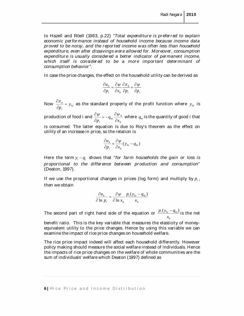
to Hazell and Röell (1983, p.22) “Total expenditure is preferred to explain economic performance instead of household income because income data proved to be noisy, and the reported income was often less than household expenditure, even after dissavings were allowed for. Moreover, consumption expenditure is usually considered a better indicator of permanent income, which itself is considered to be a more important determinant of consumption behavior”.

In case the price changes, the effect on the household utility can be derived as

ii

h

hi

h

ppxpu

Now hii

h yp

as the standard property of the profit function where hiy is

production of food i and h

hhi

i xq

p

where hiq is the quantity of good i that

is consumed. The latter equation is due to Roy’s theorem as the effect on utility of an increase in price, so the relation is

)( hihihi

h qyxp

u

Here the term ii qy shows that “for farm households the gain or loss is

proportional to the difference between production and consumption” (Deaton, 1997).

If we use the proportional changes in prices (log form) and multiply by ip ,

then we obtain

h

hihii

hi

h

xqyp

xpu )(

lnln

The second part of right hand side of the equation or h

hihii

xqyp )(

is the net

benefit ratio. This is the key variable that measures the elasticity of money-equivalent utility to the price changes. Hence by using this variable we can examine the impact of rice price changes on household welfare.

The rice price impact indeed will affect each household differently. However policy making should measure the social welfare instead of individuals. Hence the impacts of rice price changes on the welfare of whole communities are the sum of individuals’ welfare which Deaton (1997) defined as

Radi Negara 2010


h

hihii

hhhh

i xqypzx

pW )(

),(ln

Where h indicates the social value of one rupiah transfer to household h as a consequence of rice price changes. The value itself would depend on several characteristics such as living standard hx and regional or geographical

background hz .

One thing that should be noticed is that, the rice which is produced by farmer (which is called paddy) is different with the rice (milled-rice) in the market or to be consumed. The measure of benefit ratio is in money terms hence it just subtracting value of consumption from the value of sales (Deaton, 1997). However regarding the rice price changes it would need an assumption that the price of paddy and rice are parallel. The average year data in figure 1.3 seems can confirm the assumption where the movements of rice and paddy price changes are always have the same direction. As we are looking at relative changes in prices, we require that the two prices should be proportional.

Figure 1.3 The log price of milled rice and paddy in Indonesia 1980-2004 (Rp/kg)

Source: IRRI in real value of author’s calculation based on IMF GDP Deflator.

Radi Negara 2010


1.3.2 Estimation method For empirical implementation, as already shown by Deaton (1989, 1997) the technique that will be utilized to describe the relation between rice price and income distribution is the non-parametric analysis.

The h in the social welfare function is hardly measured. One of the novel

ways is to look at the pattern in which production and consumption vary with the living standard (Deaton, 1989). The household living standard can be represented by household income (expenditure) per capita. Therefore, instead of measuring the parameters of the farm household model, I prefer to examine the pattern of per capita expenditure by looking at the budget share of rice

h

hii

xqp )(

and net benefit ratio in relation to regional characteristics (rural vs

urban, islands, provinces) and various types of household (farmer vs non-farmer, producer (including self-consumption) vs seller).

First, the density function of price and income will be estimated by using kernel estimator for univariate and bivariate densities. According to Silverman (1986, p. 76) the kernel estimator is defined by

n

i

id h

xxKnh

xf1

1)(ˆ

with kernel K , bandwidth h and d is dimensional x (for univariate d =1) and the Gaussian kernel function (the standard multivariate normal density function) is

)21exp()2()( 2 xxxK Td

The univariate kernel will be used to estimate the living standard densities in urban and rural areas separately. The pattern of expenditure per capita between urban and rural will be compared in order to provide the background for the regional separation and investigate the inequality between rural and urban areas.

Joint distributions of per capita expenditure and rice budget share, and per capita expenditure and net benefit ratio will be shown by kernel bivariate estimator. The patterns of these variables will give clear pictures of how rice price changes are distributed among the households based on their living standards.

In STATA the estimation of univariate density use the ‘kdensity’ command and for bivariate densities, the commands are the spkde, spgrid and spmap program code which is developed by Pisati (2009).

Second, I will use the non-parametric regression to look more into details of density. According to Deaton (1997) non-parametric methods interpret the regression function in terms of the joint distribution,

Radi Negara 2010


dyxyfdyxyyfxyExm jj ),(/),()|()(

)(xm can be estimated by using the kernel regression estimator,

hxxK

hxxKy

xmi

n

i

in

ii

1

1)(

Basically non-parametric methods have a particular strength compare to the usual linear regression. Deaton (1997) mentions that non-parametric regressions don’t have to deal with strict assumption of parametric regression and exploring the data itself to choose their own shape of the curve. However there is still problem of bias in kernel regression estimator due to unequally spaced x’s selection (see Deaton, 1997 p.197-198). Therefore the weighted local linear regression will be applied to tackle this problem. Fan (1992) shows that locally weighted regression parameter is superior (with high efficiency) to other kernel methods. Technically from Deaton (1997) locally weighted regression can be done by first define

h

xxKh

x ii

1)(

then estimate the parameter yxXXxXx )('])('[)(ˆ 1

“where )(x is an nxn diagonal matrix with )(xi in the i-th position and the

2nx matrix X has ones in its first column and the vector x-values in its second. The predicted value of this regression at x is then the estimated value of the regression function at grid point” (Deaton, 1997 p.199) i.e.,

xxxxm )(ˆ)(ˆ)(ˆ 21 where the results will be in terms of graphic lines. The non-parametric regression will give an exact answer on who gains and who loses from rice price changes. In practice, STATA has provided locally weighted regression by command called LOWESS estimation, so we don’t have to estimate each steps manually.

Radi Negara 2010


2. Data

2.1 Sample structure

In 2000, the RAND Corporation in collaboration with the Center for Population and Policy Studies (CPPS) of the University of Gadjah Mada conducted the IFLS (Indonesian Family Life Survey). The IFLS is a multipurpose household survey that covers several questions about the farm and non-farm household economy. This cross sectional data set of 14 provinces covers around 80% of the Indonesian population (10,433 households, 39,000 individual interviews), and can be used to test the effect of the price of rice and several related government policies on the farm household economy.

Table 2.1 shows the numbers of survey households and their distribution over the country. The households are distributed over rural and urban regions. For DKI Jakarta as capital city of Indonesia, it doesn’t have any rural region. Following Deaton (1989) the analysis will be kept separated between rural and urban in order to maintain different characteristics of those two areas.

Table 2.1 Samples on IFLS 3

Code Province

Urban Rural Total

samples Population

(1990) Population

(2000)

HH City Subdis

trict HH County Subdis

trict

12 North Sumatera 306 16 51 384 14 42 690 10,256,027 11,649,655

13 West Sumatera 162 5 18 313 11 31 475 4,000,207 4,248,931

14 Riau 39 7 14 17 9 9 56

16 South Sumatera 188 7 22 327 7 38 515 6,313,074 6,899,675

18 Lampung 75 6 9 308 8 33 383 6,017,573 6,741,439

31 DKI Jakarta 853 5 42 - - - 853 8,259,266 8,389,443

32 West Java 948 26 128 940 26 155 1888 35,384,352 35,729,537

33 Central Java 541 32 99 784 29 107 1325 28,520,643 31,228,940

34 DI Yogyakarta 383 5 32 221 4 27 604 2,913,054 3,122,268

35 East Java 618 30 108 885 30 125 1503 32,503,991 34,783,640

51 Bali 204 8 13 287 8 27 491 2,777,811 3,151,162

52 West Nusa Tenggara 173 7 12 489 6 42 662

3,369,649 4,009,261

63 South Kalimantan 170 9 11 293 11 36 463

2,597,572 2,985,240

73 South Sulawesi 274 17 24 234 13 31 508 6,981,646 8,059,627

Other provinces 12 7 9 5 4 4 17

Total 4946 187 592 5487 180 707 10433 149,894,865 160,998,818

Source: IFLS3, BPS, Author’s calculation

Basically there are 13 provinces that were selected to maximize representation of the population, include the social diversity and minimize the cost of survey.

Radi Negara 2010


Even though the 1990’s population becomes the basis of sample selection, the sample size of IFLS 3 in each of the provinces is still in proportion of population in 2000. The samples are located on the island of Sumatera, Java, Kalimantan, Sulawesi, Bali and Sunda Kecil (Nusa Tenggara). Households from Riau and other provinces in table 2.1 are the previous household from IFLS 1 (1993) that lived in one of 13 provinces and then moved.

The Colums of city/county and sub-district in table 2.1 show the numbers that are included in each province. The basis of random selection within provinces is the 321 enumeration areas i.e. a nationally representative sample frame used in the 1993 SUSENAS (Strauss et al, 2004). Then households (20 from each urban and 30 from each rural) were randomly selected from those enumeration areas where the lists were obtained from regional BPS office. The household definition is “a group of people whose members reside in the same dwelling and share food from the same cooking pot (the standard BPS definition)” (Strauss et al, p.10, 2004).

In addition, IFLS datasets has some advantages which made the work load of this research more efficient. The project “Equity and Growth” of the Research Group that was partially funded by World Bank Research Committee has estimated the total household consumption from IFLS data set and measured the temporal and spatial deflator from SUSENAS in order to change them into real value (Witoelar, 2009).

The project has tried to deal with the issue of outliers and missing value. Observations at the higher end of distribution would become outliers if the difference with the next lower one was large. The missing values were replaced by taking imputations i.e. the median values taken at community level, sub-district level, or city/county level (Witoelar, 2009).

There is however no perfect imputation method. Moreover median imputation is not the best method. With normal distribution, it would give results that are not so different from mean imputation (Acuna and Rodriguez, 2004). Many large surveys, including family survey have serious problems with missing value and outliers (Acock, 2005 and Burke, 1998) and this could imply “bias estimation, distorted statistical power, and invalid conclusions” (Acock, 2005). There are a many tests to detect those problems either in a parametric or non-parametric way (see Burke, 2001). However every method to solve missing value, and to include or exclude outliers has pros and cons. Plus I cannot do a re-imputation with other better methods because the IFLS only provide total consumption data that integrated with median imputation on missing values. Therefore to estimate total consumption by myself requires numerous of work and time which I couldn’t fulfill in this research time deadline. Hence I will try to be aware and be critical in interpreting every estimation result.

Radi Negara 2010


2.2 Data Summary

Table 2.2 presents the average values of the main variables the farm household model. Following Deaton (1989) per capita expenditure (pce) will be used as the measure of household living standard. It was measured by dividing household expenditures by the number of household members. In the IFLS, household expenditures consist of food expenditure, non-food expenditures (e.g. clothing, furniture, medical, ceremonies, tax, etc.), education expenditures and housing expenditures.

From this measurement standard we can see that households in urban area are better off than rural households. The differences of living standard between urban and rural are diverse. South Sumatera, West Java and West Nusa Tenggara have urban expenditures that are more than 50% higher than those of rural hhs. While in Bali and South Kalimantan, urban households are less than 20% richer than rural households. The rural areas of West Nusa Tenggara and South Sulawesi are the poorest regions.

Table 2.2 Average of per capita expenditure (pce), rice revenue, rice consumption and budget share of rice per month

Urban Rural

Province

pce (Rp) HH Rice revenue

(Rp)

HH Rice consumption

(Rp)

Budget share of rice (%)

pce (Rp) HH Rice revenue

(Rp)

HH Rice consumption

(Rp)

Budget share of rice (%)

North Sumatera

371,616.5 11,299.1 146,642.7 11 255,599.1 68,266.55 177,413.3 19

West Sumatera

424,799.2 28,848.65 131,701.5 9 344,068.8 37,234.42 164,533.5 15

South Sumatera

426,661.2 0 94,531.92 6 231,421 75,503.18 128,060.8 14

Lampung 340,826.1 7,021.587 120,339 9 249,636.8 71,933.51 129,446.9 15

DKI Jakarta 496,626.4 1,091.548 88,277.67 5 - - - -

West Java 444,555.8 2,563.51 81,726.45 8 290,800.9 137,278.5 110,118.6 14

Central Java 401,743.6 10,568.97 83,653.13 8 283,359.3 82,983.84 91,425.9 11

DI Yogyakarta

435,707.4 38,403.51 69,239.97 7 321,723.8 90,298.06 93,595.88 11

East Java 394,745.2 31,953.25 73,467.98 8 273,168.4 86,065.72 115,841 14

Bali 370,695.5 5,707.847 97,795.3 10 321,012.8 32,749.65 118,150.7 12

West Nusa Tenggara

323,007.2 29,142.17 92,150.03 11 210,127.4 60,967.7 122,351.6 17

South Kalimantan

338,027.2 2,439.721 99,297.52 8 304,146.5 78,333.48 104,590.3 12

South Sulawesi

297,652.2 113,385.6 112,114.1 10 241,582.9 147,005.6 135,987.6 15

Source: IFLS 3, Author’s calculation.

The second variable in table 2.2 is the rice revenue of rice farmer household. This is on monthly and household basis. The farm household in IFLS can be

Radi Negara 2010


selected from criteria of land farming ownership, rented or shared land farming, or having a household member that has worked in a farm business. Rice revenues were only recorded when rice was the most valuable source of agricultural income (either crop or livestock). This surely not the ideal definition of rice farmer because then the farmer that planted paddy as their secondary crop is excluded by this criteria. The rice crop estimation also could be overvalued for farmer with rice as primary crop and undervalued for farmer with rice as secondary crop. Unfortunately there are no alternatives. Here I assume that the farm household that does not have rice/paddy as their primary crop is not a rice farm household.

The approximate amount of total production was asked on yearly basis. Therefore the rice revenue values in the table 2.2 were divided by 12 and were adjusted to real value. As expected the rural rice revenues in each of the provinces are higher than in urban regions. Most rice farmers are living in rural area, 28.9% from total rural sample, while in urban areas, only 5.7% of urban total sample are rice farmers in our definition. These percentages are lower compare to table 1.2 that shows SUSENAS data which could be due to that IFLS data only covers 80% of Indonesian population while SUSENAS covers the whole Indonesian population.

One way to examine the rice price effect is by exploring the household rice consumption pattern. We use both rice consumption and the budget share of rice. Comparing urban to rural households in each province, on average the rice consumption of urban households is lower. This is also confirmed by the budget share of rice that tends to be smaller for higher income per capita. Therefore the effect of rice price changes could be stronger for rural households welfare.

However farm household theory implies the duality of rice farmer. Even though they lose as consumer when rice price is increase, as a producer they benefit from the increase in rice revenue. The net effect then will depend on the difference between consumption and production. From table 2.2 can be derived that there are several provinces where on average, the rice production values exceeds the consumption values5. Most of these net producers live in rural areas. However a majority of regions has an average rice consumption that is higher than average rice revenue except in urban and rural area of South Sulawesi and rural area in West Java.

From this point of view, the rice price effect will potentially harm the majority of the regions. This is a preliminary analysis, because average values ignore the variations in observations. Therefore a deeper analysis will be provided in the next chapter.

5 In most provinces, the differences between rice production and consumption in monetary value of table 2.2 are very big especially if we compare with table 1.1 where the total production and consumption in quantity are almost equal. The possibility is that the price difference between paddy and milled rice is also high (see figure 1.3)

Radi Negara 2010


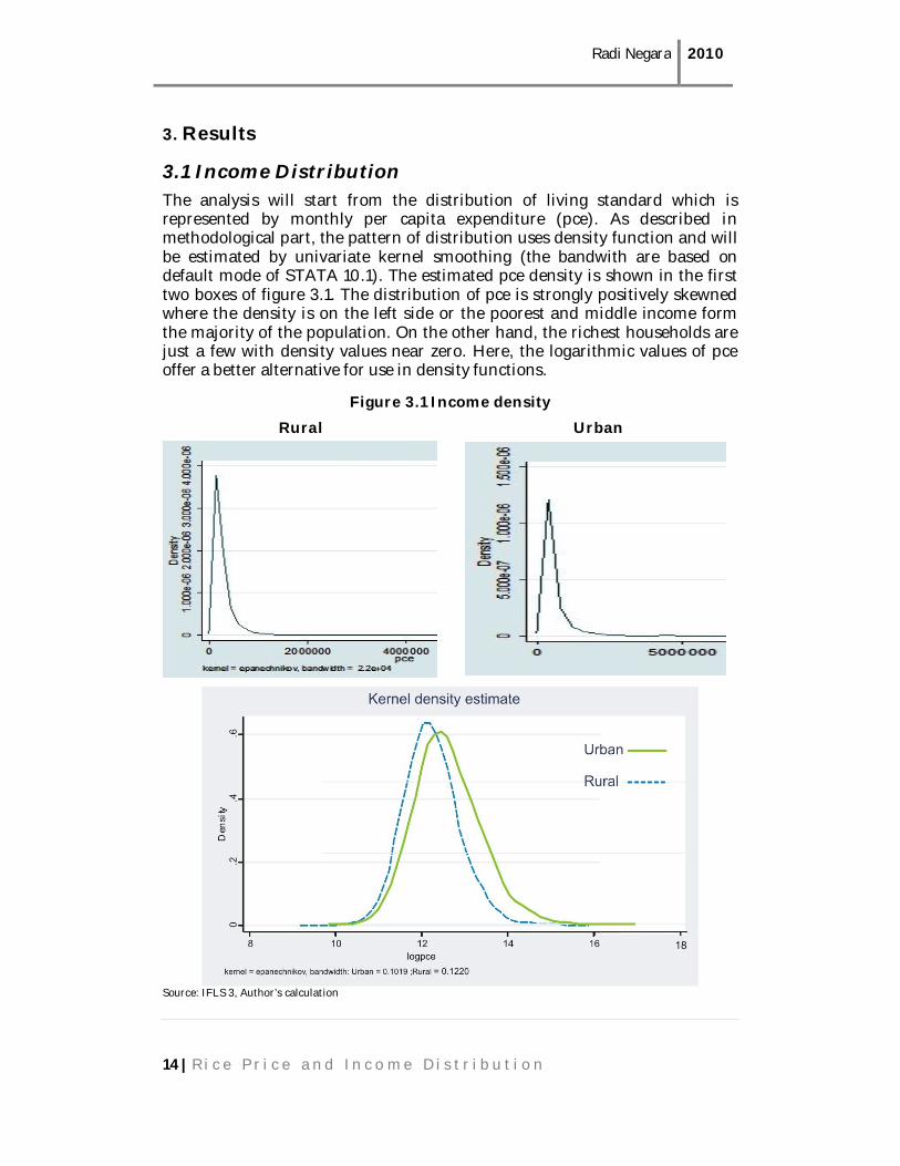
3. Results

3.1 Income Distribution

The analysis will start from the distribution of living standard which is represented by monthly per capita expenditure (pce). As described in methodological part, the pattern of distribution uses density function and will be estimated by univariate kernel smoothing (the bandwith are based on default mode of STATA 10.1). The estimated pce density is shown in the first two boxes of figure 3.1. The distribution of pce is strongly positively skewned where the density is on the left side or the poorest and middle income form the majority of the population. On the other hand, the richest households are just a few with density values near zero. Here, the logarithmic values of pce offer a better alternative for use in density functions.

Figure 3.1 Income density

Rural Urban

Source: IFLS 3, Author’s calculation

Radi Negara 2010


In the last part of figure 3.1, the distribution of pce in logarithmic (log pce) has the shape of normal distribution. This pattern gives a clearer picture to compare graphs of log pce distribution in rural and urban areas. The graphs confirm the pattern of average value of total expenditure in previous chapter. It gives a more complete picture of the differences in living standard between urban and rural areas for the whole distribution.

The two tails represent the two extreme levels of income. Most of the poor households live in the rural area, while the richest households reside in the urban area. For middle income class, the urban has a wider graph and is slightly more to the right which means that they are better off than rural middle income class. One should notice that at the level of logarithmic value of around 12, the numbers of households in rural area are higher than in urban region.

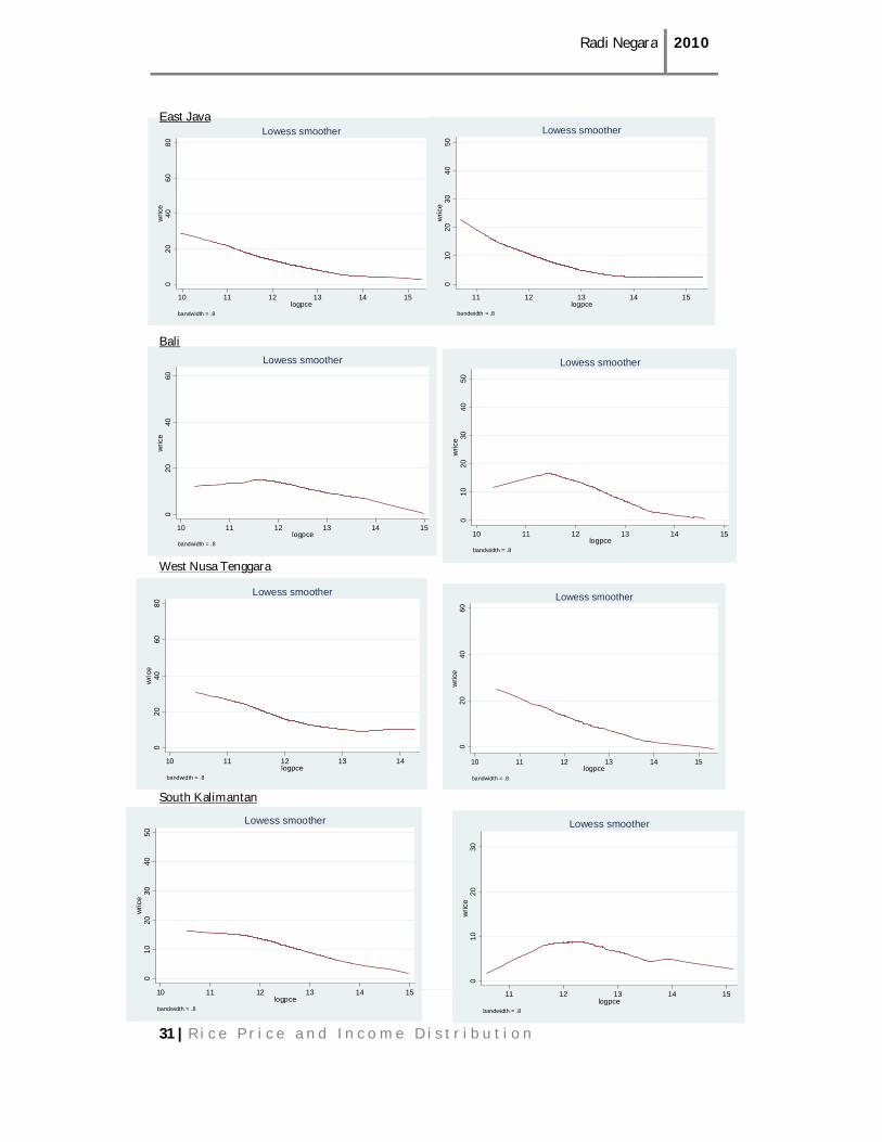
3.2 Rice Budget Share

The next estimations are relating the rice budget share (wrice) to the living standard distribution. The results are plotted in figure 3.2 where rural area is on the left and urban area is on the right. The first two diagrams are contour maps where the scale of graphs normalizes to 0-1 and the red contour shows the highest density6. For the contour map I use a very small bandwidth (0.1) with the aim to see as many as variations it can get. Here the map exhibits nicely the dispersion of rice share at all levels of living standard where for certain level of expenditure or income, the households have different rice budget share.

Despite this mixed of shapes of contours, it still possible to generalize the pattern. The red dominated contours show the negative relationship between rice share and the living standard. Either in rural or urban areas, the better your condition of living, the lower your rice share expenditure. In terms of food expenditure, the wealthier the households, instead of increasing rice consumption proportionately with income, they would prefer to increase the side dishes consumption such as meats or fish and other variations of food and other goods.

The same conclusion can also be drawn by comparing rural areas and urban areas. On looking at the group with highest density or at the whole population, the rural area which is worst off in living standard has higher level of rice budget share compare to the urban area. These confirm that the proportion of rice consumption to the total expenditure will be lower as the living standard increases.

6 To see another example which gives more clear steps, see Pisati (2009) as the author of skpde command.

Radi Negara 2010


0.2

.4.6

.8w

stap

les

8 10 12 14 16logpce

bandwidth = .8

Lowess smoother

0.2

.4.6

.8w

stap

les

10 12 14 16 18logpce

bandwidth = .8

Lowess smoother


0.2

.4.6

.8w

rice

8 10 12 14 16logpce

bandwidth = .8

Lowess smoother0

.2.4

.6w

rice

10 12 14 16 18logpce

bandwidth = .8

Lowess smoother

Figure 3.2 Living standard and rice consumption in Indonesia 2000

Rural Joint density contours Urban

Rice share averaged by log pce

Other staple food share averaged by log pce

Radi Negara 2010


However from consumer point of view, to come to a conclusion on which group will be the most affected when the rice price changes it need a fair weight that give exact measurement. Here the non-parametric regression gives better option to show the pattern in one line and with wider bandwidth (0.8) to get a softer pattern.

The second part of figure 3.2 gives sharper pattern of diversity. Surprisingly the rural poor households in average tend to have lower rice share than their counterparts in urban area. The rice share in rural area also increases from the very poor households to a certain level of income before it decreases continually until the highest level of income. As indicated by the third part of figure 3.2, the possible explanation is that most of rural households with very limited income substitute rice by other cheaper primary food such as cassava or sweet potatoes. Due to land abundance, the rural poor are able to plant alternative staple food in their backyard. In general, the urban poor households who lack the option to seek the cheaper alternative, will be the most affected group when the rice price changes.

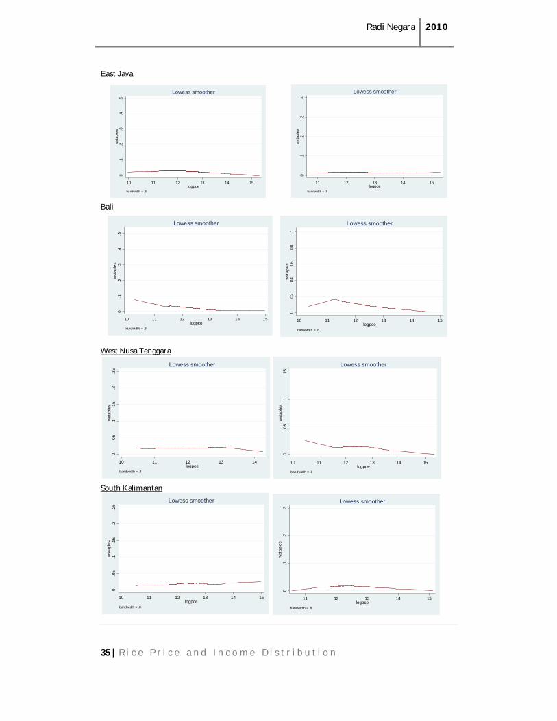
Looking at the existence of the staple food alternative, it offers a possibility to decrease the rice consumption dependency in order to minimize the rice price impact. However, this policy option can only be realized in a long term program. In terms of consumption it would be difficult to change the preference of primary food as it is already a habit across generations. According to Timmer (1971) in Indonesia, with a bad image corn and cassava are the inferior staple food as food for low income level, and even are associated with malnutrition and hunger. And on the production side, providing mass supply of alternative staple food will need many incentives for farmers to plant them as main crops.

A competitive price with rice is needed to spur alternative staple food production and consumption growth. Alternatives such as noodles or bread are more expensive because wheat as the input is mostly imported. Other alternative such as corn or cassava or sweet potato are too cheap to give profit for farmers even though this would depend on how the supply chain functions. Nowadays cassava can be processed into various food products (agribusinessweek, 2009). Therefore at least these diverse staple foods can be potential rice substitutes to minimize the rice price impact.

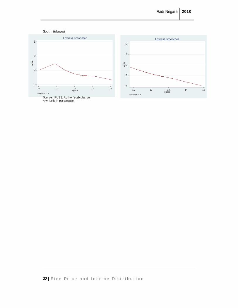
Indonesia is identical with cultural diversity including that of their food. Therefore regional details are necessary. Although rice consumption is spread in all provinces either in rural or urban areas (see Appendix B), the alternative staple food (see Appendix C) occurs in certain areas and forms a significant valuable food for the poor household group. For example in rural North Sumatera, rural and urban West Sumatera, rural South Sumatera and Lampung, rural East Java, rural and urban Bali, urban West Nusa Tenggara and rural South Sulawesi. With those differences, it is not always the urban poor that will be the biggest loser of the rice price increases. There are certain poor rural or urban groups in certain provinces that don’t see any alternative

Radi Negara 2010



of rice. As an implication, for certain areas and group of income, the rice subsidy such as rice for poor program could be over valuated and not on target. Hence, the government should consider offering alternative scheme that should be offered would be cheap complementary nutritional food for certain group that already substitute rice by other staple food. However further and deeper study is needed for this kind of alternative scheme.

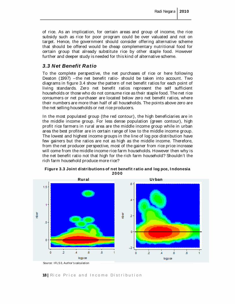
3.3 Net Benefit Ratio To the complete perspective, the net purchases of rice or here following Deaton (1997) –the net benefit ratio- should be taken into account. Two diagrams in figure 3.4 show the pattern of net benefit ratios for each point of living standards. Zero net benefit ratios represent the self sufficient households or those who do not consume rice as their staple food. The net rice consumers or net purchaser are located below zero net benefit ratios, where their numbers are more than half of all households. The points above zero are the net selling households or net rice producers.

In the most populated group (the red contour), the high beneficiaries are in the middle income group. For less dense population (green contour), high profit rice farmers in rural area are the middle income group while in urban area the best profiter are in certain range of low to the middle income group. The lowest and highest income groups in the line of log pce distribution have few gainers but the ratios are not as high as the middle income. Therefore, from the net producer perspective, most of the gainer from rice price increase will come from the middle income rice farm households. However then why is the net benefit ratio not that high for the rich farm household? Shouldn’t the rich farm household produce more rice?

Figure 3.3 Joint distributions of net benefit ratio and log pce, Indonesia 2000

Rural Urban

Radi Negara 2010


Figure 3.4 Rice production value averaged by logpce, Indonesia 2000

Rural rice farmer Urban rice farmer


Figure 3.5 Joint distributions of net benefit ratio and log cultivated farm land size, Indonesia 2000


Source: IFLS 3, Author’s calculation Figure 3.4 shows that the better household living standard, the rice revenue is higher. It means that the income does not necessarily in a relationship with benefit. If some households have high rice revenue the benefit could be small if they have high rice consumption or total consumption.

Other point of view is shown by figure 3.5. Apparently for rice farmers, per capita expenditure is not proportional to the land asset as the representation of household economy status. Figure 3.5 shows the distribution of net benefit ratio of rice farmers over their cultivated farm size (in logs). The land size is chosen as independent variable because for farmers, it might better indicate

01.

00e+

072.

00e+

073.

00e+

074.

00e+

07yr

ice

10 11 12 13 14 15logpce

bandwidth = .8

Lowess smoother

020

0000

0400

0000

6000

0008

0000

001.

00e+

07yr

ice

11 12 13 14 15logpce

bandwidth = .8

Lowess smoother

Radi Negara 2010


-10

12

34

nber

10 12 14 16 18logpce

bandwidth = .8

Lowess smoother

the farm characteristic than the per capita expenditure. In rural areas where most rice farmers live, the benefit ratio increases as their farm land increases.

The differences between two variables could be caused by the interaction with number of household members or the rice consumption. It is possible that rich farmers with vast farm land have many household members and it is still common in Indonesia for rich people to have more than one wife. The then reported rice consumption is possibly different with the real household rice expenditure. The rice consumption of their farm workers could be included which will increase their total rice expenditure.

But the question still remains, how about the loser? Figure 3.3 also shows significant density for the net consumer. Not even all rice producers benefit from rice price increases (see figure 3.5). There are rice farmers that have less production than their consumption (in monetary value).

Then the rice price increase will benefit most of the middle and rich rice farm households, while for poor rice farmers the outcome is uncertain. There are some poor rice farmers that benefit and there are some that lose. The variations among households make it difficult to draw firm conclusion on the rice price effect. To process the variations give straight answers on the rice price effect on social welfare, non-parametric regressions were conducted.

Figure 3.6 Net benefit ratio averaged by log pce, Indonesia 2000

Rural Urban


Figure 3.6 shows the net benefit ratio averaged by log per capita expenditure. According to Deaton (1997) the interpretation of non-parametric regression lines of household income and net benefit ratio are; the flat line means that all households benefit proportionately, positive slope indicate the benefit is larger when households move to better living standard and negative slope shows the benefit is better for households with lower income. These are if the line is above zero, if the line is below zero then the movement of income shows the changes of loss.

05

1015

nber

8 10 12 14 16logpce

bandwidth = .8

Lowess smoother

Radi Negara 2010


-10

12

34

nber

-10 -5 0 5 10log_lsize

bandwidth = .8

Lowess smoother

05

1015

nber

-10 -5 0 5 10log_lsize

bandwidth = .8

Lowess smoother

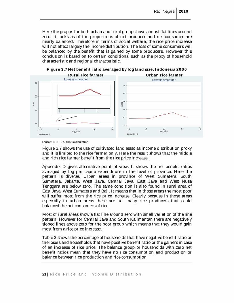
Here the graphs for both urban and rural groups have almost flat lines around zero. It looks as of the proportions of net producer and net consumer are nearly balanced. Therefore in terms of social welfare, the rice price increase will not affect largely the income distribution. The loss of some consumers will be balanced by the benefit that is gained by some producers. However this conclusion is based on to certain conditions, such as the proxy of household characteristic and regional characteristic.

Figure 3.7 Net benefit ratio averaged by log land size, Indonesia 2000



Figure 3.7 shows the use of cultivated land asset as income distribution proxy and it is limited to the rice farmer only. Here the result shows that the middle and rich rice farmer benefit from the rice price increase.

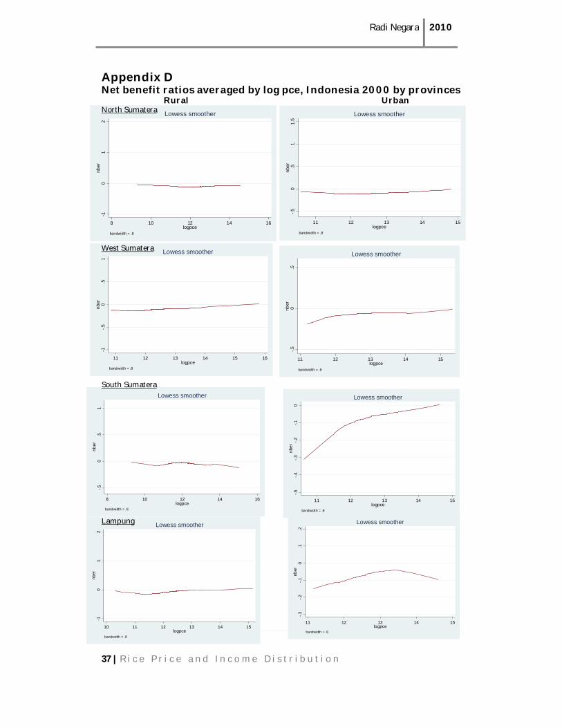
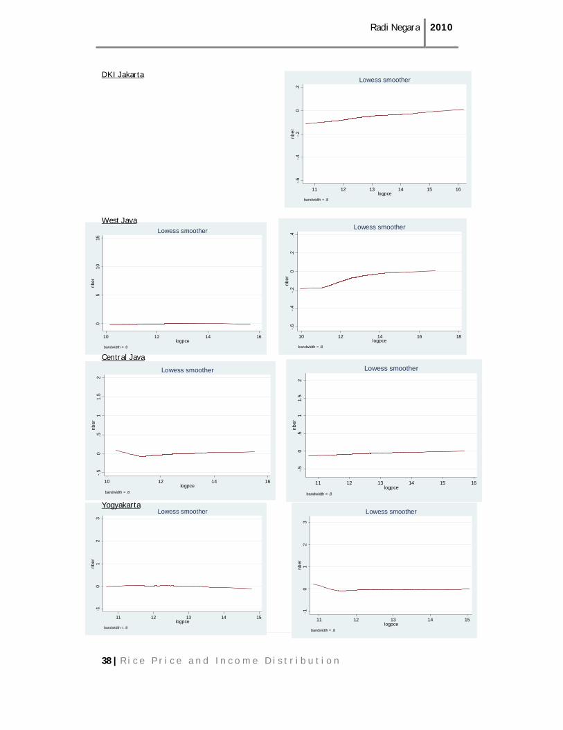
Appendix D gives alternative point of view. It shows the net benefit ratios averaged by log per capita expenditure in the level of province. Here the pattern is diverse. Urban areas in province of West Sumatera, South Sumatera, Jakarta, West Java, Central Java, East Java and West Nusa Tenggara are below zero. The same condition is also found in rural area of East Java, West Sumatera and Bali. It means that in those areas the most poor will suffer most from the rice price increase. Clearly because in those areas especially in urban areas there are not many rice producers that could balanced the net consumers of rice.

Most of rural areas show a flat line around zero with small variation of the line pattern. However for Central Java and South Kalimantan there are negatively sloped lines above zero for the poor group which means that they would gain most from a rice price increase.

Table 3 shows the percentage of households that have negative benefit ratio or the losers and households that have positive benefit ratio or the gainers in case of an increase of rice price. The balance group or households with zero net benefit ratios mean that they have no rice consumption and production or balance between rice production and rice consumption.

Radi Negara 2010


The gainers are minority in all provinces, even smaller than the balance group except in Lampung, West Nusa Tenggara and South Sulawesi. At a glance, it looks like contradictive if we compare with figure 3.6 that shows the net benefit ratio tend to balance around zero along the level of living standard. Even though they are minority, it seems that in absolute their positive net benefit ratios are higher than negative benefit ratios of other households in the same level of living standard.

Table 3: Percentage of losers and gainers from rice price increase, Indonesia 2000

Losers Gainers Balance Total

Total 69% 11% 20% 100%

Rural 70% 18% 12% 100%

Urban 68% 4% 28% 100%

North Sumatera 68% 7% 24% 100%

West Sumatera 71% 6% 22% 100%

South Sumatera 58% 14% 28% 100%

Lampung 84% 10% 6% 100%

DKI Jakarta 63% 0% 37% 100%

West Java 70% 9% 21% 100%

Central Java 67% 14% 18% 100%

DI Yogyakarta 64% 18% 18% 100%

East Java 70% 12% 18% 100%

Bali 81% 6% 13% 100%

West Nusa Tenggara 75% 15% 10% 100%

South Kalimantan 66% 16% 18% 100%

South Sulawesi 67% 24% 10% 100% Sources: IFLS3, Author’s calculation

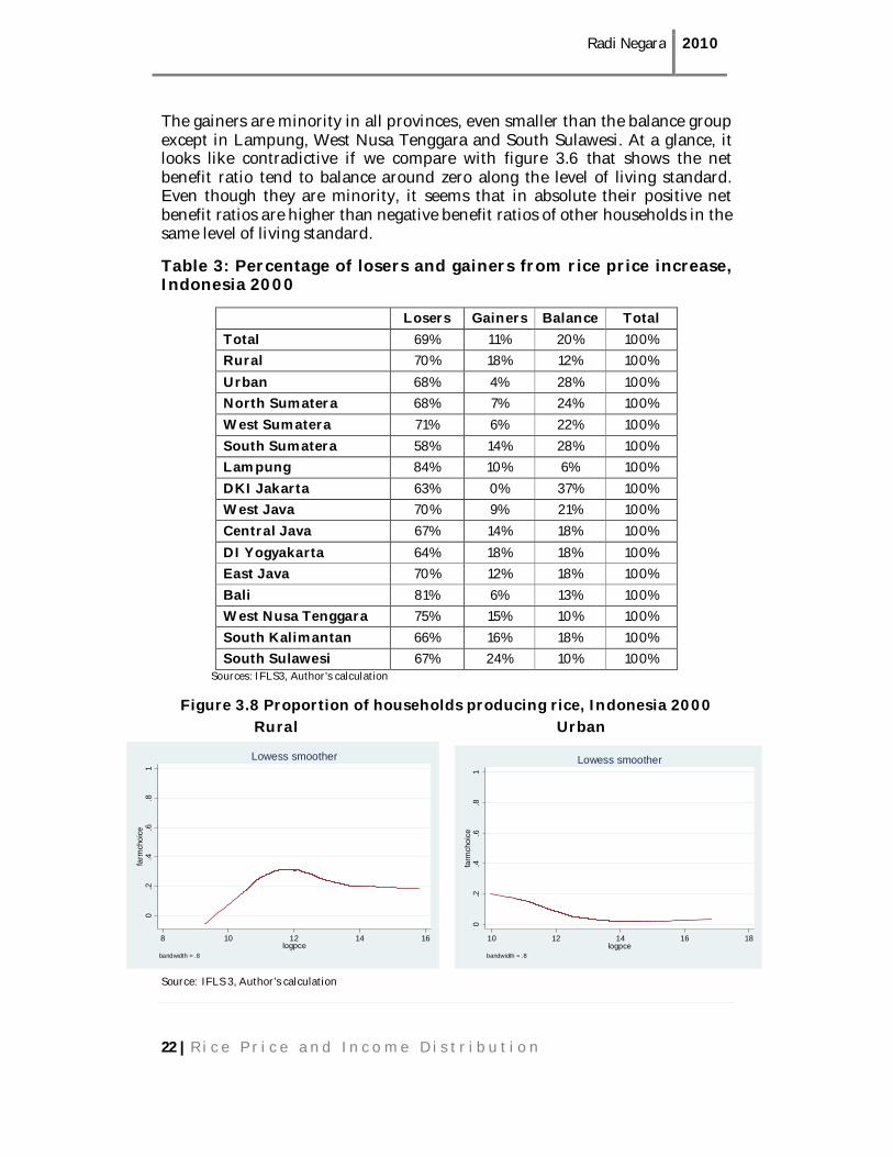
Figure 3.8 Proportion of households producing rice, Indonesia 2000

Rural Urban


0.2

.4.6

.81

farm

choi

ce

10 12 14 16 18logpce

bandwidth = .8

Lowess smoother

0.2

.4.6

.81

farm

choi

ce

8 10 12 14 16logpce

bandwidth = .8

Lowess smoother

Radi Negara 2010


Despite evidence on the predicament of poor rice farmers, figure 3.8 shows that this job is still preferable to poor household. Here the independent variable is logarithm of pce and the dependent variable is a dummy variable, equal to one in case of a rice farmer and zero if not. The graph indicates that the preference to grow rice tends to increase from low to middle income farm households, and to decline to the best-off households. This shows that growing rice is still preferred by low income households to increase their living standard to certain level. Yet, for most households the better their living standard is, the less is their tendency to grow rice.

For government the tricky policy would be how to provide cheap rice to the poor consumers and on the other side to protect poor rice farmers. In the current short term policy, the government does monopsony policy through Bulog to keep the high price for paddy and sell rice at low prices to the consumer. But then there will be other questions as to what extent this policy would impact on the productivity of the rice farmer. There is a danger of moral hazard problems with this policy which requires further study. This policy also will cost a lot of subsidy and seems to be inefficient regarding the results which high rice prices did not help poor farmers and cheap rice possibly is not on target due to variation in staple food consumption.

The alternatives policy is to liberalize rice market. Hence the high domestic rice prices will be affected by cheaper rice from Thailand or Vietnam. This will cut a lot of subsidy. However further study is needed regarding the potential negative impact to the local rice farmers.

In the long term the challenge is to promote the poor rice farmer into wealthier farmer and this means to increase the productivity. This would be a hard thing to do, considering that the limitation of Indonesia land farming nowadays. Data from the Department of Agriculture in the Agriculture Development Planning 2005-2009 mentioned that the average cultivated land per capita is only 0.09 hectare. The farm census shows that the number of poor farmer with less than 0.5 hectare farm land has increased from 10.88 million household in 1993 to 13.7 million household in 2003 (Indonesia Department of Agriculture, 2005).

Radi Negara 2010


4. Conclusion The impact of rice price changes on income distribution varies which depends on the household net benefit ratio, household characteristic and regional characteristic. In proportion the effect of rice price changes is nearly balance between gainers and losers. In case of price increase, the sufferers with negative “net benefit ratio” are spread to every household level of income, while the highest gainers mostly are the middle income household. An increase of rice price is tend to increase of poverty level, even though the numbers are not so high because poor rice farm households can benefit from rice price increase.

Rice price support does not provide full protection to the poor. High rice prices did not help poor farmers. Cheap rice possibly is not on target due to variation in staple food consumption. This could indicate an inefficiency of subsidy in current rice policy; high price for rice farmers and low price for consumer.

Therefore policy maker should improve their policy in looking which side of consumer should be protected when the rice price changes. The non-rice farm poor and middle income households should be the targets in keeping the market rice price low. The regional characteristics regarding its variation should be taken cautiously by the government in distributing cheap rice. Policy maker should take into account the different characteristic of household and region that consumer with no staple food alternative should become priority to protect when the rice price increases.

For rice farmers, the government can still implement their monopsony policy through Bulog in protecting poor rice farmer. However this policy also still cost a lot of subsidy. The potential cheapest way is to liberalize rice market where the rice import is open for private companies, despite that will need further study to analyze due to the potential impact to the local rice farmers.

However in view of the data validity, the conclusion then should be taken cautiously. There is some vagueness in imputation method for this survey. Other problems concerns about the unclear criteria of rice farmer (see chapter 2) and the validity of rice production which is only provided in value instead of quantity. It is not possible to cross check this value with the quantity of production multiplied by the market price. Therefore the net benefit ratio estimation could be under or overvalued.

The non-parametric method used gives a wider perspective for the impact of rice prices on the income distribution. The variation within household groups can be seen in detail, which shows us that the impact of any policy cannot be taken as linear and equal even for the same type of household.

Hopefully with newer survey data and more valid and detailed farm household data, more reliable conclusions of this kind of research can be reached.

Radi Negara 2010


References: Acock, A. C. (1997). Working with missing values. Family Science Review, 10, 76 -102. http://people.oregonstate.edu/~acock/growth curves/working%20with%20missing%20values.pdf

Acuna, E. and Rodriguez, C. (2004) The treatment of missing values and its effect in the classifier accuracy. In Banks, D. (Ed.), et al. Classification, Clustering and Data Mining Applications, , Berlin, Heidelberg Springer-Verlag, pp. 639–648. http://academic.uprm.edu/~eacuna/IFCS04r.pdf

Agribusinessweek (2009) Growing Cassava for Food & Profit. http://www.agribusinessweek.com/growing-cassava-for-food-profit/ Alston, J.M., K.A. Foster, and R.D. Green. (1994) "Estimating Elasticities with the Linear Approximate Almost Ideal Demand System: Some Monte Carlo Results." The Review of Economics and Statistics. 76: 351-56. http://www.jstor.org/stable/2109891

Baum, C., (2008) ”KDENS2: Stata module to estimate bivariate kernel density”. Statistical Software Components, Boston College Department of Economics. http://econpapers.repec.org/RePEc:boc:bocode:s448502.

Blanciforti, L., and Green, R., (1983). "An Almost Ideal Demand System Incorporating Habits: An Analysis of Expenditures on Food and Aggregate Commodity Groups." Review of Economics and Statistics. 65. 511-515. http://www.jstor.org/stable/1924200

BPS (2006) Profil Kemiskinan di Indonesia Maret 2006 [Indonesia Poverty Profile March 2006]. Berita Resmi Statistik. BPS, Jakarta.



BPS (2008) Keadaan Ketenagakerjaan Indonesia Februari 2008 [Indonesia Labor Condition February 2008]. Berita Resmi Statistik. BPS, Jakarta.


Burke S (1998). Missing values, outliers, robust statistics and nonparametric methods. VAMBull (1 9):22-27. http://chromatographyonline.findanalytichem.com/lcgc/Statistics+&+Data+Analysis/Missing-Values-Outliers-Robust-Statistics-and-Non-/ArticleStandard/Article/detail/4509

Byrne, P., Capps, O., Shaha, A., 1996. Analysis of food-away-from-home expenditure patterns for US households, 1982–89. Am. J. Agric. Econ. Vol.78, p.614–627.

Cui, J., (2005) “The Demand for International Message Telephone Services: A Two-Stage Budgeting Model” Review of Industrial Organization. Vol 27. No 2. p.167-183.

Radi Negara 2010


Springer Netherlands. http://www.springerlink.com/content/u65g20272hv3m175/fulltext.pdf

Deaton, A., (1997) The analysis of household surveys: microeconometric analysis for development policy Monograph, World Bank, Washington DC, 1997

Deaton, A., (1989) Rice Prices and Income Distribution in Thailand: A Non-Parametric Analysis, The Economic Journal, Vol. 99, No. 395, Supplement: Conference Papers (1989), pp. 1-37 Published by: Blackwell Publishing for the Royal Economic Society. http://www.jstor.org/stable/2234068

Deaton, A., Muellbauer, J. (1980) “An Almost Ideal Demand System”. The American Economic Review. Vol. 70. No. 3. p. 312-326. American Economic Association. http://www.jstor.org/stable/1805222

de Janvry, A., Fafchamps, M., Sadoulet, E., (1991) The Economic Journal, Vol. 101, No. 409 pp. 1400-1417 Blackwell Publishing for the Royal Economic Society http://www.jstor.org/stable/2234892

del Campo,J.C.C.M., Páez, H.J.V. (2008) The Impact of Food Price Increases on Poverty in Mexico. LACEA/IDB/WB/UNDP Network on Inequality and Poverty. http://www.nip-lac.org/uploads/H_ctor_Juan_Villarreal_P_ez.pdf

Fan, J., (1992) Design-adaptive Nonparametric Regression Journal of the American Statistical Association, Vol. 87, No. 420 (Dec., 1992), pp. 998-1004 Published by: American Statistical Association

Foster, J., Greer, J., Thorbecke, E., 1984. A class of decomposable poverty measures, Econometrica, vol.52, no.3, p.761–766.

Green, R., and J.M. Alston. (1990) "Elasticities in AIDS Models." American Journal of Agricultural Economics. 72: 442-45.

Haq, Z., Nazli, H., Meilke, K. (2008), Implications of high food prices for poverty in Pakistan,Agricultural Economics, vol.39, no.1, p. 477-484, http://econpapers.repec.org/RePEc:bla:agecon:v:39:y:2008:i:s1:p:477-484.

Herzfeld, T. (2009) Lecture 9 Economic Models: Demand Systems. Agriculture Economics Groups. Wageningen Universiteit.

IRRI world rice statistics. International Rice Research Institute. http://beta.irri.org/solutions/index.php?option=com_content&task=view&id=250

Jamal, E., Noekman, K., Hendiarto., Ariningsih, E., Askin, A. (2006) Analisis Kebijakan Penentuan Harga Pembelian Gabah [Analysis of Floor Price of Rice Policy]. Final Report 2006. Indonesia Department of Agriculture. Jakarta. http://pse.litbang.deptan.go.id/ind/pdffiles/LHP_ERZ_2006.pdf

Kontan (2008) HPP Beras 2009 Naik, Jadi Rp 4.600 per Kg [Floor Price of Rice is Increase to Rp4600/kg]. Edition:Tuesday, 30 December 2008. Jakarta http://www.kompas.com/read/xml/2008/12/30/0956309/hpp.beras.2009.naik.jadi.rp.4.600.per.kg

Radi Negara 2010


McCulloch, N. (2008) Rice Prices and Poverty in Indonesia. Bulletin of Indonesian Economic Studies, vol. 44, vo. 1, p.45–63

Pakpahan, A. (1992) Increasing the Scale of Small Farm Operations III. Indonesia. Center for Agro-Socioeconomic Research, Agency for Agricultural Research and Development, Bogor, Indonesia.

Pisati, M., (2009) "SPKDE: Stata module to perform kernel estimation of density and intensity functions for two-dimensional spatial point patterns," Statistical Software Components S456999, Boston College Department of Economics. http://ideas.repec.org/c/boc/bocode/s456999.html

P. B. R. Hazell, Ailsa Röell (1983) Rural Growth Linkages: Household Expenditure Patterns in Malaysia and Nigeria Door. International Food Policy Research Institute, Research Report 41. http://books.google.nl/books?hl=nl&lr=&id=TuxikbwlO6YC&oi=fnd&pg=PA6&dq=Rural+growth+linkages&ots=AF-zHfovHM&sig=1aoDghPBCxqlC7CWVsJQN7VUw_w#v=onepage&q=&f=false

RAND (2007) Indonesian Family Life Survey 4. http://www.rand.org/labor/family/software_and_data/FLS/IFLS/download.html

Solihin, D. (2008) Evaluasi Pelaksanaan RPJM Nasional 2004-2009. BAPPENAS, Jakarta. http://www.docstoc.com/docs/1828063/Evaluasi-Pelaksanaan-RPJM-Nasional-2004-2009

Sen, A. (1976) Poverty: An Ordinal Approach to Measurement. Econometrica, Vol.44, No.2, p.19-231.

Strauss, J., K. Beegle, B. Sikoki, A. Dwiyanto, Y. Herawati and F. Witoelar. “The Third Wave of the Indonesia Family Life Survey (IFLS3): Overview and Field Report”. March 2004. WR-144/1- NIA/NICHD. Tempointeraktif (2006) HKTI Desak Pemerintah Batalkan Impor Beras [Farmer Association Force Government to Ban the Rice Import]. Jakarta http://www.tempointeraktif.com/hg/ekbis/2006/09/05/brk,20060905-83366,id.html

Timmer, C. Peter(1971) 'Estimating Rice Consumption', Bulletin of Indonesian Economic Studies, 7: 2, 70 — 88 http://dx.doi.org/10.1080/00074917112331331852

USDA Research Service data sets. United States Department of Agriculture. http://www.ers.usda.gov/Data/

World Bank. (2006) Making the New Indonesia Work for the Poor. Washington.

Radi Negara 2010


Appendix A Program Code (figure 3.2) 1. Normalize variables in the range [0,1]

. sysuse "rural.dta", clear

. summarize logpce wrice

. clonevar x = logpce

. clonevar y = wrice

. replace x = (x-min) / (max-min)

. replace y = (y-min) / (max-min)

. mylabels 0(max/5)max, myscale((@-min) / (max-min)) local(XLAB)

. mylabels 0(max/4)max, myscale((@-min) / (max-min)) local(YLAB)

. keep x y

. save "xy.dta", replace

2. Generate a 100x100 grid

. spgrid, shape(hexagonal) xdim(100) ///

xrange(0 1) yrange(0 1) ///

dots replace ///

cells("2D-GridCells.dta") ///

points("2D-GridPoints.dta")

3. Estimate the bivariate probability density function

. spkde using "2D-GridPoints.dta", ///

xcoord(x) ycoord(y) ///

bandwidth(fbw) fbw(0.1) dots ///

saving("2D-Kde.dta", replace)

4. Display the density plot

. use "2D-Kde.dta", clear

. recode lambda (.=0)

. spmap lambda using "2D-GridCells.dta", ///

id(spgrid_id) clnum(20) fcolor(Rainbow) ///

ocolor(none ..) legend(off) ///

point(data("xy.dta") x(x) y(y)) ///

freestyle aspectratio(1) ///

xtitle(" " "logpce") ///

xlab(`XLAB') ///

ytitle("wrice" " ") ///

ylab(`YLAB', angle(0)) Source: Pisati (2009)

Radi Negara 2010


020

4060

80w

rice

11 12 13 14 15 16logpce

bandwidth = .8

Lowess smoother

020

4060

wric

e

8 10 12 14 16logpce

bandwidth = .8

Lowess smoother

010

2030

wric

e

11 12 13 14 15logpce

bandwidth = .8

Lowess smoother

020

4060

80w

rice

10 11 12 13 14 15logpce

bandwidth = .8

Lowess smoother

Appendix B Living standard and rice consumption (wricea), Indonesia 2000 by provinces

Rural Urban North Sumatera West Sumatera South Sumatera Lampung

020

4060

wric

e

11 12 13 14 15logpce

bandwidth = .8

Lowess smoother

020

4060

80w

rice

8 10 12 14 16logpce

bandwidth = .8

Lowess smoother

010

2030

4050

wric

e

11 12 13 14 15logpce

bandwidth = .8

Lowess smoother

010

2030

4050

wric

e

11 12 13 14 15logpce

bandwidth = .8

Lowess smoother

Radi Negara 2010


010

2030

4050

wric

e

11 12 13 14 15 16logpce

bandwidth = .8

Lowess smoother

020

4060

wric

e

10 12 14 16 18logpce

bandwidth = .8

Lowess smoother

020

4060

80w

rice

10 12 14 16logpce

bandwidth = .8

Lowess smoother

020

4060

wric

e

11 12 13 14 15 16logpce

bandwidth = .8

Lowess smoother

010

2030

4050

wric

e

10 12 14 16logpce

bandwidth = .8

Lowess smoother

010

2030

4050

wric

e

11 12 13 14 15logpce

bandwidth = .8

Lowess smoother

020

4060

wric

e

11 12 13 14 15logpce

bandwidth = .8

Lowess smoother

DKI Jakarta West Java Central Java Yogyakarta

Radi Negara 2010


010

2030

4050

wric

e

11 12 13 14 15logpce

bandwidth = .8

Lowess smoother

020

4060

80w

rice

10 11 12 13 14 15logpce

bandwidth = .8

Lowess smoother

010

2030

4050

wric

e

10 11 12 13 14 15logpce

bandwidth = .8

Lowess smoother

020

4060

wric

e

10 11 12 13 14 15logpce

bandwidth = .8

Lowess smoother

020

4060

wric

e

10 11 12 13 14 15logpce

bandwidth = .8

Lowess smoother

020

4060

80w

rice

10 11 12 13 14logpce

bandwidth = .8

Lowess smoother

010

2030

wric

e

11 12 13 14 15logpce

bandwidth = .8

Lowess smoother

010

2030

4050

wric

e

10 11 12 13 14 15logpce

bandwidth = .8

Lowess smoother

East Java Bali West Nusa Tenggara South Kalimantan

Radi Negara 2010


010

2030

40w

rice

11 12 13 14 15logpce

bandwidth = .8

Lowess smoother0

2040

60w

rice

10 11 12 13 14logpce

bandwidth = .8

Lowess smoother

South Sulawesi

Source: IFLS 3, Author’s calculation a: wrice is in percentage

Radi Negara 2010


Appendix C Other staples food share averaged by log pce, Indonesia 2000 by provinces

Rural Urban

North Sumatera West Sumatera

Rural Urban South Sumatera Lampung

0.2

.4.6

.8w

stap

les

11 12 13 14 15logpce

bandwidth = .8

Lowess smoother

0.2

.4.6

.8w

stap

les

8 10 12 14 16logpce

bandwidth = .8

Lowess smoother

0.0

5.1

.15

wst

aple

s

11 12 13 14 15logpce

bandwidth = .8

Lowess smoother

0.0

5.1

.15

.2.2

5w

stap

les

11 12 13 14 15 16logpce

bandwidth = .8

Lowess smoother

0.0

5.1

.15

.2.2

5w

stap

les

11 12 13 14 15logpce

bandwidth = .8

Lowess smoother

0.1

.2.3

wst

aple

s

8 10 12 14 16logpce

bandwidth = .8

Lowess smoother

0.0

5.1

.15

wst

aple

s

10 11 12 13 14 15logpce

bandwidth = .8

Lowess smoother

0.0

1.0

2.0

3.0

4.0

5w

stap

les

11 12 13 14 15logpce

bandwidth = .8

Lowess smoother

Radi Negara 2010


DKI Jakarta West Java Central Java Yogyakarta

0.1

.2.3

.4w

stap

les

11 12 13 14 15 16logpce

bandwidth = .8

Lowess smoother

0.1

.2.3

wst

aple

s

10 12 14 16 18logpce

bandwidth = .8

Lowess smoother

0.0

5.1

.15

.2.2

5w

stap

les

10 12 14 16logpce

bandwidth = .8

Lowess smoother

0.1

.2.3

.4w

stap

les

11 12 13 14 15 16logpce

bandwidth = .8

Lowess smoother

0.1

.2.3

.4w

stap

les

10 12 14 16logpce

bandwidth = .8

Lowess smoother

0.1

.2.3

.4w

stap

les

11 12 13 14 15logpce

bandwidth = .8

Lowess smoother

0.0

5.1

.15

wst

aple

s

11 12 13 14 15logpce

bandwidth = .8

Lowess smoother

Radi Negara 2010


East Java Bali West Nusa Tenggara South Kalimantan

0.1

.2.3

.4w

stap

les

11 12 13 14 15logpce

bandwidth = .8

Lowess smoother

0.0

2.0

4.0

6.0

8.1

wst

aple

s

10 11 12 13 14 15logpce

bandwidth = .8

Lowess smoother

0.1

.2.3

.4.5

wst

aple

s

10 11 12 13 14 15logpce

bandwidth = .8

Lowess smoother

0.0

5.1

.15

wst

aple

s

10 11 12 13 14 15logpce

bandwidth = .8

Lowess smoother

0.0

5.1

.15

.2.2

5w

stap

les

10 11 12 13 14logpce

bandwidth = .8

Lowess smoother

0.1

.2.3

wst

aple

s

11 12 13 14 15logpce

bandwidth = .8

Lowess smoother

0.0

5.1

.15

.2.2

5w

stap

les

10 11 12 13 14 15logpce

bandwidth = .8

Lowess smoother

0.1

.2.3

.4.5

wst

aple

s

10 11 12 13 14 15logpce

bandwidth = .8

Lowess smoother

Radi Negara 2010


South Sulawesi Source: IFLS 3, Author’s calculation

0.0

5.1

.15

.2.2

5w

stap

les

11 12 13 14 15logpce

bandwidth = .8

Lowess smoother

0.0

5.1

.15

.2.2

5w

stap

les

10 11 12 13 14logpce

bandwidth = .8

Lowess smoother

Radi Negara 2010


-10

12

nber

10 11 12 13 14 15logpce

bandwidth = .8

Lowess smoother

-.3-.2

-.10

.1.2

nber

11 12 13 14 15logpce

bandwidth = .8

Lowess smoother

-.50

.51

nber

8 10 12 14 16logpce

bandwidth = .8

Lowess smoother

-.5-.4

-.3-.2

-.10

nber

11 12 13 14 15logpce

bandwidth = .8

Lowess smoother

-1-.5

0.5

1nb

er

11 12 13 14 15 16logpce

bandwidth = .8

Lowess smoother

-.50

.5nb

er

11 12 13 14 15logpce

bandwidth = .8

Lowess smoother

-10

12

nber

8 10 12 14 16logpce

bandwidth = .8

Lowess smoother

-.50

.51

1.5

nber

11 12 13 14 15logpce

bandwidth = .8

Lowess smoother

Appendix D Net benefit ratios averaged by log pce, Indonesia 2000 by provinces

Rural Urban North Sumatera West Sumatera South Sumatera Lampung

Radi Negara 2010


-10

12

3nb

er

11 12 13 14 15logpce

bandwidth = .8

Lowess smoother

-10

12

3nb

er

11 12 13 14 15logpce

bandwidth = .8

Lowess smoother

-.50

.51

1.5

2nb

er

10 12 14 16logpce

bandwidth = .8

Lowess smoother

-.50

.51

1.5

2nb

er

11 12 13 14 15 16logpce

bandwidth = .8

Lowess smoother

05

1015

nber

10 12 14 16logpce

bandwidth = .8

Lowess smoother

-.6-.4

-.20

.2.4

nber

10 12 14 16 18logpce

bandwidth = .8

Lowess smoother

-.6-.4

-.20

.2nb

er

11 12 13 14 15 16logpce

bandwidth = .8

Lowess smootherDKI Jakarta West Java Central Java Yogyakarta

Radi Negara 2010


-.50

.51

nber

10 11 12 13 14 15logpce

bandwidth = .8

Lowess smoother

-.3-.2

-.10

.1.2

nber

11 12 13 14 15logpce

bandwidth = .8

Lowess smoother

-.50

.51

1.5

nber

10 11 12 13 14logpce

bandwidth = .8

Lowess smoother

-.50

.51

nber

10 11 12 13 14 15logpce

bandwidth = .8

Lowess smoother

-.50

.51

nber

10 11 12 13 14 15logpce

bandwidth = .8

Lowess smoother

-.50

.51

nber

10 11 12 13 14 15logpce

bandwidth = .8

Lowess smoother

-10

12

34

nber

10 11 12 13 14 15logpce

bandwidth = .8

Lowess smoother

-10

12

34

nber

11 12 13 14 15logpce

bandwidth = .8

Lowess smootherEast Java Bali West Nusa Tenggara South Kalimantan

Radi Negara 2010


-10

12

3nb

er

10 11 12 13 14logpce

bandwidth = .8

Lowess smoother

01

23

4nb

er

11 12 13 14 15logpce

bandwidth = .8

Lowess smootherSouth Sulawesi


Documents

The Effect of Rice Price Changes on the Income