NBER WORKING PAPER SERIES

THE EFFECT OF PROVIDING PEER INFORMATION ON RETIREMENT SAVINGSDECISIONS

John BeshearsJames J. ChoiDavid Laibson

Brigitte C. MadrianKatherine L. Milkman

Working Paper 17345http://www.nber.org/papers/w17345

NATIONAL BUREAU OF ECONOMIC RESEARCH1050 Massachusetts Avenue

Cambridge, MA 02138August 2011

We thank Aon Hewitt and our corporate partner for conducting the field experiment and providingthe data. We are particularly grateful to Pam Hess, Mary Ann Armatys, Diane Dove, Barb Hogg, DianaJacobson, Larry King, Bill Lawless, Shane Nickerson, and Yan Xu, some of our many contacts atAon Hewitt. We thank Sherry Li and seminar participants at Berkeley, Cornell, Stanford, Wharton,the NBER Summer Institute, the Harvard Business School / Federal Reserve Bank of Boston ConsumerFinance Workshop, and the Behavioral Decision Research in Management Conference for their insightfulfeedback. Michael Buckley, Yeguang Chi, Christina Jenq, John Klopfer, Henning Krohnstad, andEric Zwick provided excellent research assistance. Beshears acknowledges financial support froma National Science Foundation Graduate Research Fellowship. Beshears, Choi, Laibson, and Madrianacknowledge individual and collective financial support from the National Institute on Aging (grantsR01-AG-021650, P01-AG-005842, and T32-AG-000186). This research was also supported by theU.S. Social Security Administration through grant #19-F-10002-9-01 to RAND as part of the SSAFinancial Literacy Research Consortium. The findings and conclusions expressed are solely thoseof the authors and do not represent the views of SSA, any agency of the Federal Government, RAND,or the National Bureau of Economic Research. See the authors’ websites for lists of their outside activities.

NBER working papers are circulated for discussion and comment purposes. They have not been peer-reviewed or been subject to the review by the NBER Board of Directors that accompanies officialNBER publications.

© 2011 by John Beshears, James J. Choi, David Laibson, Brigitte C. Madrian, and Katherine L. Milkman.All rights reserved. Short sections of text, not to exceed two paragraphs, may be quoted without explicitpermission provided that full credit, including © notice, is given to the source.

The Effect of Providing Peer Information on Retirement Savings DecisionsJohn Beshears, James J. Choi, David Laibson, Brigitte C. Madrian, and Katherine L. MilkmanNBER Working Paper No. 17345August 2011, Revised August 2014JEL No. D03,D14,D83,D91

ABSTRACT

We conducted a field experiment in a 401(k) plan to measure the effect of disseminating informationabout peer behavior on savings. Low-saving employees received simplified plan enrollment or contributionincrease forms. A randomized subset of forms stated the fraction of age-matched coworkers participatingin the plan or age-matched participants contributing at least 6% of pay to the plan. We document anoppositional reaction: the presence of peer information decreased the savings of non-participants whowere ineligible for 401(k) automatic enrollment, and higher observed peer savings rates also decreasedsavings. Discouragement from upward social comparisons seems to drive this reaction.

John BeshearsHarvard Business SchoolBaker Library 439Soldiers FieldBoston, MA 02163and NBERjbeshears@hbs.edu

James J. ChoiYale School of Management135 Prospect StreetP.O. Box 208200New Haven, CT 06520-8200and NBERjames.choi@yale.edu

David LaibsonDepartment of EconomicsLittauer M-12Harvard UniversityCambridge, MA 02138and NBERdlaibson@gmail.com

Brigitte C. MadrianHarvard Kennedy School79 JFK StreetCambridge, MA 02138and NBERBrigitte_Madrian@Harvard.edu

Katherine L. MilkmanUniversity of Pennsylvania3730 Walnut Street561 Jon M. Huntsman HallPhiladelphia, PA19104kmilkman@wharton.upenn.edu

An online appendix is available at:http://www.nber.org/data-appendix/w17345/

The Effect of Providing Peer Information on Retirement Savings Decisions

JOHN BESHEARS, JAMES J. CHOI, DAVID LAIBSON, BRIGITTE C. MADRIAN, AND

KATHERINE L. MILKMAN*

July 27, 2014

Journal of Finance, forthcoming

ABSTRACT

We conducted a field experiment in a 401(k) plan to measure the effect of disseminating information about peer behavior on savings. Low-saving employees received simplified plan enrollment or contribution increase forms. A randomized subset of forms stated the fraction of age-matched coworkers participating in the plan or age-matched participants contributing at least 6% of pay to the plan. We document an oppositional reaction: the presence of peer information decreased the savings of non-participants who were ineligible for 401(k) automatic enrollment, and higher observed peer savings rates also decreased savings. Discouragement from upward social comparisons seems to drive this reaction.

*Harvard University and NBER, Yale University and NBER, Harvard University and NBER, Harvard University and NBER, and University of Pennsylvania. We thank Aon Hewitt and our corporate partner for conducting the field experiment and providing the data. We are particularly grateful to Pam Hess, Mary Ann Armatys, Diane Dove, Barb Hogg, Diana Jacobson, Larry King, Bill Lawless, Shane Nickerson, and Yan Xu, some of our many contacts at Aon Hewitt. We thank Campbell Harvey (the Editor), an Associate Editor, an anonymous referee, Hunt Allcott, Sherry Li, and seminar participants at Brigham Young University, Case Western Reserve University, Cornell University, New York University, Norwegian School of Economics, Stanford University, University of California Berkeley, University of Maryland, University of Pennsylvania, the NBER Summer Institute, the Harvard Business School / Federal Reserve Bank of Boston Consumer Finance Workshop, and the Behavioral Decision Research in Management Conference for their insightful feedback. Michael Buckley, Yeguang Chi, Christina Jenq, John Klopfer, Henning Krohnstad, Michael Puempel, Alexandra Steiny, and Eric Zwick provided excellent research assistance. Beshears acknowledges financial support from a National Science Foundation Graduate Research Fellowship. Beshears, Choi, Laibson, and Madrian acknowledge individual and collective financial support from the National Institutes of Health (grants P01-AG-005842, R01-AG-021650, and T32-AG-000186). This research was also supported by the U.S. Social Security Administration through grant #19-F-10002-9-01 to RAND as part of the SSA Financial Literacy Research Consortium. The findings and conclusions expressed are solely those of the authors and do not represent the views of SSA, any agency of the Federal Government, or RAND. See the authors’ websites for lists of their outside activities.

1

In 1980, 30 million U.S. workers actively participated in employer-sponsored defined

benefit (DB) retirement savings plans, and 19 million actively participated in employer-

sponsored defined contribution (DC) retirement savings plans. By 2011, participation in DB

plans had nearly halved to 17 million workers, while DC plan participation had skyrocketed to

74 million workers.2 The shift from DB plans, which set contribution levels and investment

allocations on behalf of employees, to DC plans, which allow employees to choose from a

complex array of possible contribution levels and investment allocations, has arrived amidst

concerns that workers are not equipped to make well-informed savings choices (Mitchell and

Lusardi, 2011). Employers have become increasingly interested in programs designed to help

employees make good choices in DC plans. This paper studies such a program.

We use a field experiment to investigate the effect of a peer information intervention on

retirement savings choices. Peer information interventions involve disseminating information

about what a target population’s peers typically do. By sharing this information, it may be

possible to teach people that a certain behavior is more common than they had previously

believed, motivating those people to engage in the behavior more themselves. This approach has

been dubbed “social norms marketing” and is used at approximately half of U.S. colleges in an

effort to reduce student alcohol consumption (Wechsler et al., 2003).

There are several theoretical reasons why peer information interventions may succeed at

moving behavior towards the peer-group average. An individual may mimic peers because their

behavior reflects private information relevant to the individual’s payoffs (Banerjee, 1992;

Bikhchandani, Hirshleifer, and Welch, 1992; Ellison and Fudenberg, 1993). Another possibility

is that the intervention provides information about social norms from which deviations are costly

due to a taste for conformity, the risk of social sanctions, identity considerations, or strategic

complementarities (Asch, 1951; Festinger, 1954; Akerlof, 1980; Bernheim, 1994; Akerlof and

Kranton, 2000; Glaeser and Scheinkman, 2003; Benjamin, Choi, and Strickland, 2010;

Benjamin, Choi, and Fisher, 2010). Finally, individuals may directly derive utility from relative

consumption (Abel, 1990).

A growing empirical literature documents that peer effects indeed play a role in financial

decisions when peers interact with each other organically. Peers affect retirement saving

2 Source: U.S. Department of Labor Employee Benefits Security Administration, Private Pension Plan Bulletin Historical Tables and Graphs, Table E8, June 2013.

2

outcomes (Duflo and Saez, 2002 and 2003), stock market participation (Hong, Kubik, and Stein,

2004; Brown et al., 2008), corporate compensation and merger practices (Bizjak, Lemmon, and

Whitby, 2009; Shue, 2013), entrepreneurial risk-taking (Lerner and Malmendier, 2013), and

general economic attitudes such as risk aversion (Ahern, Duchin, and Shumway, 2013).3 Peer

information interventions such as the one we study are designed to harness the power of these

peer effects to influence behavior.

Many studies find that peer information interventions cause behavior to more closely

conform to the disseminated peer norm.4 Our field experiment, however, yields a surprising

result. Peer information interventions can generate an oppositional reaction: information about

the high savings rates of peers can lead low-saving individuals to shift away from the peer norm

and decrease their savings relative to a control group that did not receive peer information. Our

evidence suggests that this effect is driven in part by peer information causing some individuals

to become discouraged, making them less likely to increase their savings rates.

We conducted our experiment in partnership with a large manufacturing firm and its

retirement savings plan administrator. Employees received different letters depending on their

401(k) enrollment status. Employees who had never participated in the firm’s 401(k) plan were

mailed Quick Enrollment (QE) letters, which allowed them to start contributing 6% of their pay

to the plan with a pre-selected asset allocation by returning a simple reply form. Employees who

had previously enrolled but were contributing less than 6% of their pay received Easy Escalation

(EE) letters, which included a nearly identical reply form that could be returned to increase their

contribution rate to 6%. Previous work has shown that these simplified enrollment and

3 Hirshleifer and Teoh (2003) review the literature on herding and related phenomena in financial markets. For evidence of peer effects in other domains, see Cialdini, Reno, and Kallgren (1990), Case and Katz (1991), Besley and Case (1994), Hershey et al. (1994), Foster and Rosenzweig (1995), Glaeser, Sacerdote, and Scheinkman (1996), Bertrand, Luttmer, and Mullainathan (2000), Kallgren, Reno, and Cialdini (2000), Sacerdote (2001), Munshi (2004), Munshi and Myaux (2006), Sorensen (2006), Gerber, Green, and Larimer (2008), Grinblatt, Keloharju, and Ikäheimo (2008), Kuhn et al. (2011), Narayanan and Nair (2013), and Chalmers, Johnson, and Reuter (forthcoming). Manski (2000) provides an overview of issues in the social interaction literature. 4 For example, providing information about peers moves behavior towards the peer norm in domains such as entrée selections in a restaurant, contributions of movie ratings to an online community, small charitable donations, music downloads, towel re-use in hotels, taking petrified wood from a national park, and stated intentions to vote (Cai, Chen, and Fang, 2009; Chen et al., 2010; Frey and Meier, 2004; Salganik, Dodds, and Watts, 2006; Goldstein, Cialdini, and Griskevicius, 2008; Cialdini et al., 2006; Gerber and Rogers, 2009). However, Beshears et al. (2013) find that disseminating short printed testimonials from peers is not effective at increasing conversion from brand-name prescription drugs to lower-cost therapeutic equivalents.

3

contribution escalation mechanisms significantly increase savings plan contributions (Choi,

Laibson, and Madrian, 2009; Beshears et al., 2013).

We assigned the QE and EE mailing recipients to one of three randomly selected

treatments. The mailing for the first randomly selected treatment included information about the

savings behavior of coworkers in the recipient’s five-year age bracket (e.g., employees at the

firm between the ages of 20 and 24, employees between the ages of 25 and 29, etc.). The mailing

for the second randomly selected treatment contained similar information about coworkers in the

recipient’s ten-year age bracket (e.g., employees at the firm between the ages of 20 and 29). The

mailing for the third randomly selected treatment contained no peer information and therefore

served as a control condition. For the QE recipients, the two peer information mailings stated the

fraction of employees in the relevant age bracket who were already enrolled in the savings plan.

For the EE recipients, the two peer information mailings stated the fraction of savings plan

participants in the relevant age bracket contributing at least 6% of their pay on a before-tax basis

to the plan.

Employees in our study naturally fall into four subpopulations distinguished along two

dimensions: QE recipients versus EE recipients, and employees who were automatically enrolled

at a 6% contribution rate unless they opted out (non-union workers at this firm) versus

employees who were not enrolled unless they opted into the plan (union workers at this firm).

Table I summarizes the key features of these four subpopulations. We distinguish along the first

dimension because the QE and EE mailings make different requests of recipients: initial

enrollment at a pre-selected contribution rate and asset allocation in the case of QE, and only an

increase to the pre-selected contribution rate in the case of EE. The second dimension is

important because it affects selection into our sample. Employees with a 6% contribution rate

default had to actively opt out of their default to a contribution rate below 6% in order to be

eligible for QE or EE, so no QE or EE recipient with this default was completely passive before

the mailing. Similarly, employees with a 0% contribution rate default had to opt out of their

default to a positive contribution rate below 6% in order to become eligible for EE.5 But in order

to be eligible for QE, employees with a 0% contribution rate default had to be completely

passive. This last subpopulation contains some employees who genuinely wanted to contribute

5 If they later returned their contribution rate to 0%, they would still be eligible for EE.

4

nothing to the 401(k) and some employees who were contributing nothing simply because of

inertia. Prior research shows that the inertial group is likely to be large (Madrian and Shea, 2001;

Choi et al., 2002 and 2004; Beshears et al., 2008).6 Because people who are contributing nothing

to the 401(k) simply because of inertia are likely to have weaker convictions about their optimal

savings rate than people who have actively chosen to contribute little, we expected QE recipients

with a 0% contribution rate default to be the subpopulation most susceptible to the peer

information intervention that we studied.

In the taxonomy of Harrison and List (2004), our study is a “natural field experiment,”

since subjects never learned that they were part of an experiment. We use administrative plan

data to track contribution rate changes during the month following our mailing.

We measure the average effect of the presence of peer information by comparing how

much more the peer information treatment groups increased their contribution rates than the

control group. We also independently estimate the effect of the magnitude of the peer

information value that employees saw. To do this, we exploit two sources of variation in the peer

information value. First, two employees of the same age were exposed to different peer

information values if one was randomly assigned to see information about coworkers in her five-

year age bracket and the other to see information about coworkers in her ten-year age bracket.

Second, two employees who are similar in age but on opposite sides of a boundary separating

adjacent five-year or adjacent ten-year age brackets would see different peer information values.

We find that among QE recipients with a 0% contribution rate default—those whom we

expected to be most susceptible to our information treatment—receiving peer information

significantly reduced the likelihood of subsequently enrolling in the plan from 9.9% to 6.3%, a

decrease of approximately one-third. These recipients’ enrollment was also decreasing in the

magnitude of the peer information value communicated. A one percentage point increase in the

reported fraction of coworkers already enrolled in the plan significantly reduced the enrollment

rate by 1.8 percentage points and significantly reduced the average before-tax contribution rate

change by 0.11% of income (which is one-fifth of the average contribution rate change among

control QE recipients with a 0% contribution default).

6 Prior to the mailing, the plan participation rate was 70% for employees with a non-enrollment default and 96% for employees with a 6% contribution rate default. The latter figure does not include employees with less than 90 days of tenure, since they are likely to have had automatic enrollment pending.

5

We do not find statistically significant evidence that the peer information intervention on

average altered the savings behavior of the other three subpopulations that had previously opted

out of their default. There is some indication (at the 10% significance level) that the magnitude

of the peer information value reported matters for these subpopulations. Among QE recipients

who had previously opted out of a 6% contribution rate default, a one percentage point increase

in the reported fraction of coworkers already enrolled in the plan increased the enrollment rate by

1.1 percentage points and increased the average before-tax contribution rate change by 0.06% of

income; both of these changes are about 1.5 times the relevant control group mean. Among EE

recipients who had opted out of a 6% contribution rate default, a one percentage point increase in

the reported fraction of participants contributing at least 6% of their pay to the plan increased

before-tax contribution rate changes by 0.07% of income—about one-fourth of the relevant

control group mean.

The finding that QE recipients with a 0% contribution rate default respond negatively to

peer information by decreasing their likelihood of enrolling in the savings plan is surprising, but

there is some precedent for perverse unintended “boomerang effects” (Clee and Wicklund, 1980;

Ringold, 2002) from peer information interventions. Schultz et al. (2007) find that among

households with low initial energy consumption, a treatment group that received information

about the energy consumption of nearby residences engaged in less energy conservation than a

control group that did not receive such information.7 Bhargava and Manoli (2011) document that

households eligible for the Earned Income Tax Credit are less likely to take up the credit when

they are told that overall take-up rates are high.8

Relative to these studies, an important contribution of our experiment is that it provides

evidence distinguishing between two possible forces behind boomerang effects: negative belief

updates and oppositional reactions. The boomerang effects in previous field experiments could

be driven by negative belief updates—individuals learning that the promoted behavior is less

7 Allcott (2011), Costa and Kahn (2013), and Ayres, Raseman, and Shih (2013) also examine household responses to information about neighbors’ energy consumption, but they do not find boomerang effects. 8 In related studies, Fellner, Sausgruber, and Traxler (2013) document that peer information regarding tax compliance can have positive or negative effects on compliance depending on the subpopulation studied. Carrell, Sacerdote, and West (2013) find unintended effects in another kind of peer intervention that attempted to use peer influence to improve the academic performance of the lowest ability students. Ashraf, Bandiera, and Lee (2014) find that the anticipation of relative performance information reduces performance among low ability students in a community health worker training program.

6

common than they previously believed and decreasing their own engagement in the behavior as a

result (Schultz et al., 2007). In contrast, it is unlikely that our boomerang effects are driven by

negative belief updates. Using randomized variation in the peer participation value shown to

individuals, we find that QE recipients with a 0% contribution rate default are less likely to

enroll in the savings plan when they see that a higher fraction of their peers are participating in

the plan. Instead of shifting their behavior towards their updated beliefs about the peer norm,

individuals shift their behavior away from the updated beliefs. We label such a response an

oppositional reaction.

We analyze treatment effect heterogeneity to better understand the drivers of oppositional

reactions. Motivated by recent evidence that relative income comparisons within workplace peer

groups can reduce job satisfaction for low-income workers (Card et al., 2012), we split

employees in our experiment into two groups based on whether they are above or below the

median income of the firm’s employees in the given employee’s U.S. state. We find that the

oppositional reaction among QE recipients with a 0% default is concentrated among employees

with low relative incomes. This result raises the possibility that information about peers’ savings

choices discourages low-income employees by making their relative economic status more

salient, reducing their motivation to increase their savings rates and generating an oppositional

reaction. Employees with low relative income in the experiment’s other three subpopulations

also exhibit more negative responses to peer information than employees with high relative

income, although the statistical significance of these interactions is not as strong. In addition, we

find evidence that some employees become discouraged when they learn that a savings rate that

they find challenging has already been attained by many of their peers.

Discouragement from upward social comparisons is unlikely to be the only factor that

drives oppositional reactions, but it should be a consideration for policymakers or managers

contemplating peer information interventions because it is potentially present in other contexts

given the ubiquity of relative status concerns. Our field experiment highlights one channel

through which the unintended consequences of financial decision-making interventions can

overwhelm the intended consequences (see also Carlin, Gervais, and Manso, 2013).

The paper proceeds as follows. Section I provides background information on the firm we

study. Section II describes our experimental design, and Section III describes our data. Section

7

IV presents our empirical results, and Section V discusses possible mechanisms driving our

findings. Section VI concludes.

I. Company Background

The company that ran our field experiment is a manufacturing firm with approximately

15,000 U.S. employees. About a fifth of the employees are represented by one of five unions. In

general, unionized workers are employed on the manufacturing shop floor, although not all shop

floor workers are unionized. The firm offers both defined benefit (DB) and defined contribution

(DC) retirement plans to its employees. The details of the DB plans vary according to an

employee’s union membership, but a typical employee receives an annual credit of 4% to 6% of

her salary in a cash balance plan, as well as interest credit on accumulated balances. Upon

retirement, the employee receives an annuity based on the notional balance accrued in the plan.

The details of the DC plan, which is the focus of our study, also depend on an employee’s

union membership. In general, employees do not need to meet a minimum service requirement

before becoming eligible for the plan. Participants can contribute up to 50% of their eligible pay

to the plan on a before-tax basis, subject to IRS limits.9 For most employees, the firm makes a

matching contribution proportional to the employee’s own before-tax contribution up to a

threshold. These matching contributions vest immediately. Table II describes the matching

formulas that apply to different employee groups. After-tax contributions to the plan are also

allowed but not matched. All employees can allocate plan balances among 21 mutual funds,

eleven of which are target date retirement funds. Employer stock is not an investment option.

On January 1, 2008, all non-union employees not already contributing to the 401(k) plan

were automatically enrolled at a before-tax contribution rate of 6% of pay unless they opted out

or elected another contribution rate.10 The default investment for automatically enrolled

employees was the target date retirement fund whose target retirement date was closest to the

employee’s anticipated retirement date. Non-union employees hired after January 1, 2008 were

also subject to automatic enrollment 60 days after hire unless they actively opted out. Automatic

enrollment was not implemented for unionized employees until January 1, 2009—after our

9 In 2008, the year of the experiment, the annual contribution limit was $15,500 for workers younger than 50 and $20,500 for workers older than 50. 10 Employees were informed in advance that they would be automatically enrolled unless they opted out.

8

sample period ends—because the collective bargaining negotiations necessary to effect the

change did not take place until the fall of 2008.

II. Experimental Design

The peer information intervention targeted non-participating and low-saving U.S.

employees who were at least 20 years old and at most 69 years old as of July 31, 2008.11 “Non-

participants” were defined as employees who were eligible for but had never enrolled in the

401(k) plan as of July 14, 2008. Two groups of non-participants were excluded from the

intervention. The first group is employees who receive a special pension benefit in lieu of an

employer match.12 The second group is employees with a 6% default contribution rate who were

within the first 60 days of their employment at the company on July 14, 2008 and had not opted

out of automatic enrollment; these employees were likely to be automatically enrolled soon after

the intervention date, so the intervention would serve little purpose for them. “Low savers” were

defined as employees who were enrolled in the 401(k) plan but whose before-tax contribution

rate was less than both their employer match threshold and 6% as of July 14, 2008.13 The

majority of employees in our experiment (72%) have a match threshold of 6%, but the match

threshold varies by union status and is less than 6% for some unionized employees and greater

than 6% for others (see Table II).14

We used a stratified randomization scheme to allocate intervention-eligible employees to

three equally sized treatment groups. We first sorted employees into bins based on age as of July

31, 2008, plan participation status (enrolled or not enrolled), administrative grouping within the

firm, and employer match structure (and therefore union status and contribution rate default).

11 Employees younger than 20 or older than 69 years of age were excluded from the intervention because there are so few employees in these categories that reporting peer information about these age groups could potentially divulge the savings decisions of individual employees. 12 Only 52 employees receive this special pension benefit but otherwise met the criteria for inclusion in the intervention. 13 We did not consider after-tax contribution rates when classifying low savers. Approximately 9% of plan participants make after-tax contributions, and approximately 9% of the employees we classified as low savers were making after-tax contributions at the time of the experiment. If we had limited the intervention to employees whose combined before-tax and after-tax contribution rates were less than both their employer match threshold and 6%, approximately 7% of the low savers would have been excluded. 14 One match formula limits employer matching contributions to a maximum of $325 per year. We did not observe the dollar amount of matching contributions as of July 14, 2008, so the definition of low savers did not exclude employees who had reached the maximum. The results of our analysis do not change meaningfully if all low savers who faced this match formula are dropped from the sample.

9

Within each of these bins, employees were randomly assigned to receive no peer information,

information about the savings behavior of peers in their five-year age bracket, or information

about the savings behavior of peers in their ten-year age bracket. Note that all of the 5-year

brackets had end points at ages 24, 29, 34, etc. In other words, all subjects between ages 20 and

24 in the 5-year peer treatment saw the same peer information. Likewise, all of the 10-year

brackets had end points at ages 29, 39, 49, etc. In other words, all subjects between ages 20 and

29 in the 10-year peer treatment saw the same peer information. Psychology research indicates

that the effect of social comparisons on behavior is most powerful when the reference group is

similar to the target individual on one or more dimensions, such as age (Jones and Gerard, 1967;

Suls and Wheeler, 2000).

On July 30, 2008, Quick Enrollment and Easy Escalation mailings were sent to target

employees, implying that employees probably received these mailings between August 1 and

August 4, 2008. Both the QE and EE mailings gave a deadline of August 22, 2008 for returning

the forms, but this deadline was not enforced. Appendices A, B, C, and D show sample QE and

EE letters.

Non-participants received a QE mailing, which described the benefits of enrollment in

the 401(k) plan, especially highlighting the employer matching contribution.15 By checking a box

on the form, signing it, and returning it in the provided pre-addressed postage-paid envelope,

employees could begin contributing to the plan at a 6% before-tax rate invested in an age-linked

target date retirement fund. Employees were reminded that they could change their contribution

rate and asset allocation at any time by calling their benefits center or visiting their benefits

website. The mailing sent to employees in the peer information treatments additionally displayed

the following text: “Join the A% of B-C year old employees at [company] who are already

enrolled in the [plan].” Letters sent to employees in the no peer information control condition

simply omitted this sentence. The number A was calculated using data on all savings-plan-

eligible employees in the five-year or ten-year age bracket applicable to the recipient. These

participation rates, reported in Table III, ranged from 77% to 93%. The numbers B and C are the

boundaries of the relevant five-year or ten-year age bracket.

15 Information on employer contributions varied according to the match structure facing the individual employee.

10

Low savers received EE mailings, which also emphasized that employees were forgoing

employer matching contributions.16 A low-saving employee could increase her before-tax

contribution rate to 6%, invested according to her current asset allocation, by completing the

form and returning it in the provided pre-addressed postage-paid envelope. Like the QE

mailings, the EE mailings reminded recipients that they could change their contribution rate or

asset allocation through their benefits call center or website. The EE peer information text, which

did not appear in the mailings to employees in the no peer information control condition, read:

“Join the D% of B-C year old [plan] participants at [company] who are already contributing at

least 6% to the [plan].” Data on all plan participants in the relevant five-year or ten-year age

bracket were used to calculate D, which ranged from 72% to 81% (see Table III).

Due to technological constraints in the processing of QE and EE forms, all QE and EE

reply forms offered only a 6% contribution rate option. Every employee with a 6% contribution

rate default had a 6% match threshold, but the match threshold differed from 6% for 77% of

mailing recipients with a 0% contribution rate default. The 6% contribution rate on the QE and

EE forms could have been less appealing to employees with a different match threshold. Within

the group of recipients with a 0% default, we have analyzed those with a match threshold other

than 6% separately from those with a match threshold of 6%. The peer information treatment

effect estimates are similar across these subsamples, although the standard errors of the estimates

for the 6% threshold group are large because of the small sample size.

III. Data

Our data were provided by Aon Hewitt, the 401(k) plan administrator. The data include a

cross-sectional snapshot of all employees in our experiment on July 14, 2008, just prior to our

intervention. This snapshot contains individual-level data on each employee’s plan participation

status, contribution rate, birth date, administrative grouping within the firm, employer match

structure, union membership, and contribution rate default. A second cross-section contains the

new plan enrollments and contribution rate changes of employees between August 4, 2008 and

September 8, 2008—right after the mailing was sent. The final cross-section contains employees’

gender, hire date, and 2008 salary, which we annualize for employees who left the firm before

16 Again, information about employer contributions was personalized.

11

the end of 2008. In Section V, when we analyze treatment effect heterogeneity, we augment our

data set with information on the state of residence and 2008 salary of all employees who were

active at the firm (including those not in our experiment) as of July 14, 2008, as well as

information on the monthly history of before-tax contribution rates for each employee.

IV. Effects of Providing Peer Information

We divide the discussion of our main empirical results into five parts. First, in Section

IV.A, we discuss the characteristics of the employees who received mailings. Second, in Section

IV.B, we analyze the effect of providing peer information in the QE mailing by comparing the

savings choices of peer information QE treatment groups to those of the control group that

received the QE mailing with no peer information. Third, in Section IV.C, we restrict our

attention to the peer information QE treatment groups and examine the response to the

magnitude of the peer information value in the mailing. Fourth, in Section IV.D, we examine the

impact of the peer information given in the EE mailings. And finally, in Section V, we discuss

possible explanations for the perverse peer information effects we observe among QE recipients

with a 0% contribution rate default.

A. Employee Characteristics

Table IV presents summary statistics for the sample that received mailings, broken out by

the type of mailing (QE or EE), contribution rate default (0% or 6%), and the type of peer

information received. The majority of the sample is male, although this fraction varies

considerably across the different subpopulations: 66% among QE recipients with a 0% default,

76% among QE recipients with a 6% default, 55% among EE recipients with a 0% default, and

68% among EE recipients with a 6% default. The average age is 41 years, and average tenure is

high—9 years among QE recipients with a 0% default, 7 years among QE recipients with a 6%

default, and 11 years in both EE subpopulations. Mean annual salary is lowest among QE

recipients with a 0% default (about $38,000) and highest among EE recipients with a 6% default

(about $57,000). Issues surrounding relative salaries may play a role in explaining differences in

responses to peer information across the four groups, a topic to which we return in Section V.

Among the two EE subpopulations, average initial before-tax contribution rates are about 2%.

12

B. Effect of Providing Peer Information in Quick Enrollment

To estimate the effect of providing peer information in the QE mailing, we compare the

savings choices of peer information QE treatment groups to those of the control group that

received no peer information. The first two columns of Table V list, by contribution rate default,

the fraction of employees in each QE treatment group who enrolled in the savings plan between

August 4, 2008 and September 8, 2008. The last two columns report the average before-tax

contribution rate change during the same time period as a percent of income for each QE

treatment group, again broken out by contribution rate default.17 Note that the contribution rate

changes are almost exactly equal to 6% of the enrollment rates because the QE response cards do

not permit contribution rates other than 6%.18 We report results both in terms of enrollment rates

and in terms of contribution rate changes because the two measures are both useful for

understanding economic magnitudes. In addition, we wish to be consistent with our presentation

of the EE subpopulation results, for which the simple relationship between the two measures

does not hold. To statistically test the effect of providing peer information, we pool the five-year

and ten-year age bracket peer information treatments (row 4 of Table V).

We first look at the non-participants with a 0% contribution rate default. This is the sub-

population that we expected to have the most malleable retirement savings choices. Among this

group, 6.3% of employees who were given peer information enrolled in the plan, while 9.9% of

those whose mailings did not include peer information enrolled in the plan, a statistically

significant difference of 3.6 percentage points. This implies that peer information provision

reduces savings plan enrollment by a third. The difference in enrollment rates corresponds to a

20 basis point reduction in the average before-tax contribution rate change as a percent of

income, a difference that is significant at the 10% level.

In contrast, we do not find evidence that providing peer information on average affects

non-participants who previously opted out of automatic enrollment at a 6% default contribution

rate. There was a 2.7% enrollment rate and a 15 basis point before-tax contribution rate increase

within the pooled peer information treatments versus a 0.7% enrollment rate and a 4 basis point

17 Individuals who ceased employment at the firm between August 4, 2008 and September 8, 2008 are treated as if their participation status and contribution rate on their departure date continued unchanged until September 8, 2008. 18 QE recipients could choose alternative contribution rates by using the benefits website or calling the benefits office, but the QE response card was probably more convenient.

13

before-tax contribution rate increase within the control group without peer information. The

differences between these two arms are not statistically significant.

Table VI analyzes the average effect of providing peer information in the QE mailings

within an ordinary least squares regression framework. The sample is non-participants who

received QE mailings. In the first two columns, the dependent variable is binary, taking a value

of one if the employee initiated savings plan participation between August 4, 2008 and

September 8, 2008;19 in the next two columns, the dependent variable is the change in the

employee’s before-tax contribution rate during the same time period. The regressions control for

gender, log tenure, log salary, and a linear spline in age with knot points every five years starting

at age 22½.20 The regression-adjusted impact of providing peer information is qualitatively and

quantitatively similar to the effect estimated from comparing means in Table V. Including peer

information decreases enrollment by 4.0 percentage points and reduces the change in the before-

tax contribution rate by 22 basis points for non-participants with a 0% contribution rate default,

while it has positive but insignificant effects on non-participants with a 6% contribution rate

default. Interestingly, for QE recipients with a 0% default, the regression coefficients on log

tenure are strongly negative. For QE recipients with a 6% default, the regression coefficients on

log tenure are also negative but not statistically significant. One possible interpretation for this

result is that individuals who have been employed at the firm for a long time but have never

enrolled in the savings plan are people who strongly believe that it is not optimal for them to

participate in the plan.

C. Effect of the Peer Information Value’s Magnitude in Quick Enrollment

To examine how the magnitude of the peer information value received by employees

affected responsiveness to the QE mailing, we limit our attention to the employees who were in

the two peer information QE treatments. An important confound our analysis must address is the

19 We report the estimates from linear probability regressions for the binary dependent variables instead of probit or logit regressions because of problems with perfect predictability. Our flexible age controls sometimes perfectly predict failure, requiring us to drop observations from probit or logit regressions. Adjusting the sample for each regression specification would make it difficult to compare results across specifications, and using a common minimal sample for all specifications could potentially give a misleading picture of the results. Thus, we report the results of linear probability regressions, which allow us to maintain a consistent sample and include all observations. 20 As noted in Table IV, salary information is missing for a small number of employees. We exclude these employees from regression samples throughout the paper. We use a linear spline in age instead of age group dummy variables in Table VI to be consistent with Table VII.

14

“reflection problem” (Manski, 1993). Because our experiment provided employees with peer

information related to their five-year or ten-year age brackets, the peer information value embeds

not only information about the peer group but also information about the age-related

characteristics of the mailing recipient. Throughout our analysis, we therefore study the

relationship between responsiveness to the mailing and the magnitude of the peer information

value while controlling for a flexible function of age—specifically, an age spline with knot

points every five years starting at age 22½.

Our empirical strategy identifies the effect of the peer information value’s magnitude

using two sources of variation. First, two employees of the same age may see different peer

information values if one is randomly assigned to receive information about her five-year age

bracket and the other is randomly assigned to receive information about her ten-year age bracket.

Second, two employees who are nearly identical in age may see different peer information values

if their ages are on opposite sides of a boundary separating two adjacent five-year or ten-year age

brackets.

Table VII presents results from our baseline regression specification for analyzing the

impact of the peer information value’s magnitude. The coefficient estimates are from ordinary

least-squares regressions for the sample of non-participants who received QE mailings with peer

information. The outcomes of interest are the same as in Table VI—enrollment in the savings

plan or the change in the employee’s before-tax contribution rate between August 4, 2008 and

September 8, 2008—as are the other regression controls.

For non-participants with a 0% contribution rate default, a one percentage point increase

in the reported fraction of coworkers participating in the plan results in a statistically significant

1.8 percentage point decrease in the probability of enrolling in the plan and a statistically

significant 11 basis point lower change in the before-tax contribution rate. To put these estimates

in perspective, the peer information values received by non-participants range from 77% to 93%,

a difference of 16 percentage points (Table III). This implies an enrollment rate and before-tax

contribution rate change that differ by 28 percentage points and 1.7% of income, respectively,

between employees who receive the lowest and the highest peer information values—a very

large difference relative to the 9.9% enrollment response and 0.6% before-tax contribution rate

change of QE recipients with a 0% default who received no peer information (Table V). Note

that these estimates cannot be directly compared to the estimates in Table VI, as the regressions

15

reported in Table VI measure the effect of the presence of peer information, while the

regressions reported in Table VII measure the effect of the magnitude of the peer information

value received, conditional on receiving peer information.

In contrast, among non-participants with a 6% default, a one percentage point increase in

the peer information value results in a 1.1 percentage point increase in the enrollment rate and a

6 basis point higher increase in the contribution rate, although these effects are significant only at

the 10% level. Note the complementarity of the results in Tables VI and VII. For non-

participants with a 0% default, receiving peer information reduces the response rate to the QE

mailings on average (Table VI), and receiving a peer information value with a higher magnitude

further reduces the QE response rate (Table VII). For QE recipients with a 6% default, receiving

peer information leads to a small but insignificant increase in the response rate on average (Table

VI), and the response rate also increases in the magnitude of the peer information value (Table

VII).

Table VIII shows the importance of the two sources of variation in the peer information

value used to generate the results in Table VII. To facilitate comparison, the first column

reproduces the peer information value coefficient estimates from Table VII. The coefficients in

the second column of Table VIII are estimated by adding to the baseline regression specification

a set of five-year age bracket dummies that correspond to the age brackets in the five-year age

bracket peer information treatment. With the inclusion of these dummies, the effect of the peer

information value is no longer identified using discontinuities across age bracket boundaries;

rather, identification comes entirely from differences between employees in the five-year versus

ten-year age bracket peer information treatments. The peer information coefficients in this

specification are slightly larger than in the baseline specification and retain the same qualitative

level of statistical significance.

The regression specification presented in the last column of Table VIII excludes the five-

year age group dummies used in the second column and instead estimates different linear splines

in age for employees in the five-year versus ten-year age bracket peer information treatments.

Here, identification comes only from comparing employees on opposite sides of an age bracket

boundary at which the peer information value jumps discontinuously. Under this specification,

the peer information value coefficients do not change sign, but they are smaller in magnitude and

lose their statistical significance. Hence, the effects estimated in the baseline specification from

16

Table VII are largely driven by the differences in peer information values between the five-year

and ten-year age bracket peer information treatments.

In Table IX, we investigate the robustness of our peer information value results to the

manner in which we control for age in our regressions. The first row presents the peer

information value coefficients from our baseline specifications in Table VII to facilitate

comparison. In the second row, we replace the original linear spline (knot points every five

years) with a linear spline featuring knot points every 2½ years, starting at age 22½. This spline

is more flexible and hence gives a sense of whether the structure imposed by the original spline

produces misleading results. The coefficients on the peer information value do not change

meaningfully with the more flexible spline, and their statistical significance strengthens for

employees with a 6% contribution rate default.

One additional element that varied across the QE mailings was the fund in which

employee contributions would be invested absent any other election by the employee. (This was

not a factor in the EE mailings, since all employees currently contributing to the plan had a

preexisting asset allocation.) This default fund was a target date retirement fund (e.g., Fund

2020) chosen according to the recipient’s anticipated retirement age and thus varying

systematically with age. Although we think it is unlikely that employees would respond to the

mailings differentially depending on the target date retirement fund offered, we nonetheless try

to account for this possibility by including dummy variables in the regressions for the exact

target date retirement fund mentioned in the mailings. As shown in the third row of Table IX,

incorporating these controls does not change our main results.

The specifications in the last two rows of Table IX are designed to address another set of

issues. The two sources of identifying variation in the peer information value are associated with

an employee’s position within an age bracket. Two employees of the same age who are randomly

assigned to the five-year versus ten-year age bracket peer information treatments differ not only

in the peer information values they see, but also in the set of peers for whom those values are

defined, with one group (the five-year group) more narrowly defined than the other. Similarly,

two employees on opposite sides of a boundary separating adjacent five-year or ten-year age

brackets are exposed to different peer information values but are also in different situations

relative to their peer groups, with one older than most of her peer group and the other younger.

To partially control for these factors, we add to our regressions variables capturing an

17

individual’s position relative to her peer information comparison group. The regressions reported

in the fourth row of Table IX include linear and squared terms for the difference in years

between the employee’s age and the mean age in her peer group; the regressions reported in the

fifth row of Table IX include linear and squared terms for the employee’s percentile rank in age

within her peer group. All coefficient estimates for the QE recipients with a 0% contribution rate

default are qualitatively similar to the baseline coefficient estimates. For the QE recipients with a

6% contribution rate default, the coefficients remain similar in magnitude but lose significance

even at the 10% level when we control for the difference between the employee’s age and her

peer group’s mean age.

D. Effect of Providing Peer Information in Easy Escalation

We now turn our attention to the impact of providing peer information to the low savers

who received the EE mailings. The first two columns of Table X list the fraction of low savers,

separately by their contribution rate default, who increased their before-tax contribution rate

between August 4, 2008 and September 8, 2008. The last two columns of Table X report the

average before-tax contribution rate change during the same time period. The last row in Table X

shows that the differences between the groups who did and did not receive peer information are

close to zero and insignificant for both 0% and 6% default contribution rate participants.

Table XI reports the OLS-adjusted average impact of providing peer information in EE.

In the first two columns, the dependent variable is a binary variable taking a value of one if the

employee increased her before-tax contribution rate between August 4, 2008 and September 8,

2008; in the next two columns, the dependent variable is the change in the employee’s before-tax

contribution rate during the same time period. In addition to the controls used in Table VI for the

QE recipients, the regressions for the EE recipients include a full set of indicator variables for

each employee’s before-tax contribution rate on July 14, 2008—two weeks prior to the mailing.

The results in Table XI are qualitatively similar to the raw differences reported in Table X:

receiving peer information has a negligible and statistically insignificant effect on savings

responses on average.

Table XII presents regressions that identify the impact of the peer information value’s

magnitude in the EE mailings. The dependent variables are the same as in Table XI. As we did in

the corresponding analysis for QE, we restrict the regression sample to EE recipients who were

18

given peer information. We find that the peer information value’s magnitude has a positive but

insignificant effect on the probability of increasing one’s before-tax contribution rate. The peer

information value’s magnitude also has an insignificant effect on the before-tax contribution rate

change for recipients with a 0% contribution rate default, but a positive and marginally

significant effect for recipients with a 6% contribution rate default. For the latter group, a one

percentage point increase in the peer information value results in a 7 basis point higher increase

in the before-tax contribution rate.

V. Mechanisms Driving the Effects of Peer Information

The negative response of non-participants with a 0% contribution rate default (unionized

employees) to the peer information in QE mailings is surprising. This contrary reaction is

probably not due to learning that coworkers had a lower plan participation rate than expected,

since the enrollment rate and contribution rate changes of non-participants with a 0% default

varied inversely with the magnitude of the peer information value they received. Instead, the

boomerang effect among QE recipients with a 0% default appears to be an oppositional reaction.

In this section, we discuss the mechanisms that may be driving the oppositional reaction.

The evidence suggests that peer information is discouraging and demotivating for some

subpopulations of employees. In particular, discouragement from being compared to peers who

have higher economic status seems to play a role, as the negative response to peer information is

concentrated among individuals who have salaries that are low in the pay distribution of the

firm’s employees in the individual’s state. There is also some evidence that employees can be

discouraged when a goal that is difficult for them to attain is revealed to be a goal that many

peers have achieved. EE recipients with a 0% default reacted more negatively to peer

information if they initially had a low contribution rate rather than a high contribution rate,

making the goal of increasing to a 6% contribution rate harder to reach.

Our experiment was not specifically designed to test these explanations for the effect of

peer information, so our analysis of treatment effect heterogeneity must be interpreted with

caution. Nonetheless, issues of low relative status and difficult-to-achieve goals arise naturally in

many settings, so this pattern of responsiveness is potentially relevant for other contexts in which

peer information interventions might be deployed.

19

A. Relative Salary and Discouragement from Peer Information

Recent research by Card et al. (2012) indicates that job satisfaction is affected by an

employee’s rank within the salary distribution of that employee’s peers. Card et al. randomly

assigned employees of the University of California to receive or not to receive information about

a website that disclosed the pay of all University of California employees. Among employees

below the median pay for their occupation category (i.e., faculty versus staff) within their

department, the information treatment had a negative effect on job satisfaction, while there was

no significant effect for employees above the median pay for their occupation category within

their department. Relative pay concerns are quite local. For staff (who constitute over 80% of the

sample), being below the campus-wide median staff pay had smaller negative effects than being

below their department’s median staff pay.

Drawing on these findings, we test how the peer information effect in our experiment

varies with an employee’s salary rank among local coworkers.21 Employees are likely to have

some knowledge, through both formal and informal workplace communication channels, of their

positions in the local pay distribution at the firm. Having one’s savings choices compared to

coworkers’ savings choices in our experiment may serve as a reminder of relative economic

standing, creating feelings of discouragement and thereby triggering an oppositional reaction

among employees with low relative income. Larger peer savings numbers would exacerbate

discouragement by increasing the size of the perceived economic gap between the low-income

employee and his coworkers.22

Our data are not as detailed as the University of California data, so we calculate an

employee’s rank within the salary distribution for all employees at the firm in the same state.23

This peer group includes employees who were not part of our experiment but excludes

employees who were not active at the firm as of July 14, 2008. Two states account for half of the

21 We thank an Associate Editor for suggesting this analysis. 22 One might wonder why a higher peer information number wouldn’t also create more discouragement among high-income employees. See Price et al. (1994) and Sloman, Gilbert, and Hasey (2003) for a discussion of why negative information is more likely to discourage people who are already low-status to begin with. 23 We do have some limited information about administrative groupings at the firm, but these groupings do not appear to correspond to meaningful peer groups. Nonetheless, we have calculated salary rank within administrative grouping and experimented with using it for analyzing heterogeneous treatment effects. In general, the results are directionally similar but attenuated relative to the results using salary rank among employees at the firm within the same state.

20

employees in the experiment, but 23 other states account for the remaining employees.24 Internet

Appendix Table I reports the distribution of employees in our experiment across within-state

income quartiles. Employees in our experiment disproportionately fall in the lower quartiles of

the distribution, especially in the case of employees with a 0% default.

We begin by studying the reaction to peer information among QE recipients with a 0%

default. To estimate heterogeneity in the effect of the presence of peer information, we augment

the regression specifications from Table VI with two additional explanatory variables: an

indicator for being below the median income among active employees at the firm in the same

state and the interaction between that indicator and the indicator for receiving peer information.

The first two columns of Table XIII display the results.

The coefficients on the uninteracted dummy for receiving peer information show that QE

recipients with a 0% default and high relative income have a small positive but insignificant

response to the presence of peer information. The coefficient on the interaction term, however, is

negative and statistically significant at the 10% level in both columns. Peer information causes

QE recipients with a 0% default and low relative income to decrease their enrollment rate by 5.2

percentage points more and decrease their before-tax contribution rate by 29 basis points of pay

more than QE recipients with a 0% default and high relative income.

Turning to heterogeneity in the effect of the peer information value’s magnitude in Quick

Enrollment, we expand the set of explanatory variables in the Table VII regression specifications

to include the indicator for having an income below the median among active employees at the

firm in the same state, the interaction between the below-median income indicator and the peer

information value received (the participation rate among employees in the relevant age group),

and the interaction between the below-median income indicator and all elements of the age

spline. It is necessary to allow separate age splines for the high and low relative income

employees so that the effect of the peer information value is identified only using variation

generated by discontinuities around age group boundaries and differences between the five-year

and ten-year age group peer information values.

The last two columns of Table XIII show that for QE recipients with a 0% default and

high relative income, a one percentage point increase in the peer information value increases the

24 We do not know the state of three employees in our experiment, so we assign them to the most common state.

21

likelihood of enrolling in the savings plan by 1.0 percentage point and increases the before-tax

contribution rate change by 6 basis points of pay, although neither effect is statistically

significant. For low relative income employees, however, the effect of a one percentage point

increase in the peer information value is 2.8 percentage points more negative for the likelihood

of enrolling and 17 basis points more negative for the before-tax contribution rate change. Both

of these interactions are statistically significant at the 5% level.

In sum, the oppositional reaction we identified among QE recipients with a 0% default is

present only among employees with low income relative to other employees at the firm in the

same state. This pattern suggests that discouragement from upward social comparisons may play

a role in generating the oppositional reaction to peer information in our experiment. Further

evidence in favor of this hypothesis is found in Table XIV, which shows that the treatment

interactions with being in the bottom half of the firm-wide salary distribution are insignificant,

with point estimates that are smaller in magnitude or of the opposite sign compared to the

treatment interactions with being in the bottom half of the firm’s state-specific salary

distribution. Recall that Card et al. (2012) find that employees are most concerned about their

salary rank relative to local coworkers, so vulnerability to discouragement from peer

comparisons should depend more on where the employee stands in the local firm wage

distribution than in the firm-wide wage distribution. Furthermore, employees are more likely to

be unaware of their location in the firm-wide wage distribution than in the local wage

distribution. We have also explored treatment interactions with being in the bottom half of the

overall state-wide pay distribution (which includes individuals who do not work for the firm) and

treatment interactions with having a salary below $30,000. As shown in Internet Appendix

Tables II and III, none of these interactions is significant.

Internet Appendix Tables IV through VII show analogous regressions for the other three

subpopulations, QE recipients with a 6% default and EE recipients with a 0% or a 6% default.

We generally find the same patterns of a negative peer information treatment interaction with

having below-median income among other employees at the firm in one’s state and a weaker

treatment interaction with having below-median income in the firm-wide distribution. The

interactions with having below-median income among other employees at the firm in one’s state

are not always statistically significant, but for each of the three subpopulations, there is at least

one negative interaction with either the presence of peer information or the peer information

22

value that is significant at the 10% level or better, and no significant positive interactions. One

interesting pattern is that in these three subpopulations, unlike among QE recipients with a 0%

default, being below the median local income does not tend to cause employees to move away

from the peer norm. Rather it merely attenuates the positive reaction to peer information found

among above-median-income employees. A possible interpretation of this difference is that the

type of employee who takes an active role in his or her savings (and thus ends up in these three

subpopulations) is less prone to discouragement from upward comparisons.

B. Difficult Goals and Discouragement from Peer Information

While discouragement caused by upward socioeconomic comparisons seems to

contribute to negative reactions to peer information, discouragement driven by other related

mechanisms may simultaneously be at work. In particular, the psychology literature documents

that setting goals for individuals can motivate increased effort and achievement in tasks ranging

from problem solving to wood chopping, especially when the goals are challenging (Locke et al.,

1981; Mento, Steel, and Karren, 1987; Gollwitzer, 1999; Heath, Larrick, and Wu, 1999; Locke

and Latham, 2002). But learning that a goal one finds extremely difficult has already been

achieved by many of one’s peers may damage one’s self-esteem, making the goal feel more

unattainable. When goals are too difficult, people are more likely to reject them and to perform

poorly (Motowidlo, Loehr, and Dunnette, 1978; Mowen, Middlemist, and Luther, 1981; Erez and

Zidon, 1984; Lee, Locke, and Phan, 1997).

We have no observable variation in how challenging QE recipients might have viewed

the suggested 6% contribution rate to be, since all QE recipients had an initial contribution rate

of 0%. But EE recipients had starting contribution rates that varied from 0% to 5%. We

conjecture that EE recipients who initially had a lower contribution rate are more likely than EE

recipients who initially had a higher contribution rate to view the suggested 6% contribution rate

as a challenging goal.25 Internet Appendix Table VIII shows the contribution rate distribution of

EE recipients with a 0% default and a 6% default immediately before the experiment was

launched. The distributions are not perfectly uniform, but there is a meaningful number of

25 We thank an anonymous referee for suggesting this analysis.

23

employees in each sample at each contribution rate from 0% to 5%.26 We augment the regression

specifications in Table XI by including the interaction between the indicator for receiving peer

information and an indicator for having an initial contribution rate of 0%, 1%, or 2%. Indicators

for each of the six possible initial contribution rates are already included as explanatory

variables, omitting one to avoid collinearity with the constant.

In Table XV, columns 1 and 3 report the results for EE recipients with a 0% default, who

are the EE group most similar to the QE recipients with a 0% default. Consistent with the

hypothesis that the oppositional reaction among QE recipients with a 0% default is driven in part

by peer information interacting negatively with a difficult suggested goal, the estimated

coefficients on the interaction between the dummy for receiving peer information and the

dummy for having a low initial contribution rate are negative and statistically significant at the

10% level. Employees with high initial contribution rates respond to the presence of peer

information with a 3.8 percentage point increase in their likelihood of increasing their

contribution rates and an 18 basis points of pay increase in their before-tax contribution rate

change. The former estimate is not statistically significant, and the latter estimate is significant at

the 10% level. Employees with low initial contribution rates have a response to peer information

that is 8.7 percentage points more negative for the likelihood of a contribution rate increase and

38 basis points of pay more negative for the before-tax contribution rate change.

However, not all employees are demotivated when they learn that many of their peers

have achieved a difficult goal. Columns 2 and 4 of Table XV show that EE recipients with a 6%

default who have low initial contribution rates have a somewhat more positive response to peer

information than EE recipients with the same default and high initial contribution rates. The

effect on the binary indicator of whether the recipient increased his before-tax contribution rate is

not significant, but the effect on the average before-tax contribution rate change is significant at

the 10% level. For some subpopulations, learning that many peers achieved a challenging goal is

perhaps an encouraging signal of one’s own ability to achieve this goal.

In Internet Appendix Table IX, we examine the robustness of the findings in Table XV

by estimating separate treatment effects from the presence of peer information for each of the six

26 An employee with a 0% contribution rate is not considered a non-participant and therefore receives an Easy Escalation mailing instead of a Quick Enrollment mailing if that employee previously had a contribution rate higher than 0%.

24

possible initial contribution rates. The results broadly corroborate the patterns we observe when

grouping the 0%, 1%, and 2% contribution rates together and the 3%, 4%, and 5% contribution

rates together. We have also investigated how EE recipients with low initial contribution rates

differ from EE recipients with high initial contribution rates in their responses to the magnitude

of the peer information value. Internet Appendix Table X shows the results from regressions that

expand the Table XII specifications by including the interaction between the dummy for having a

low initial contribution rate and the peer information value as well as the interaction between the

dummy for having a low initial contribution rate and all elements of the age spline. The results

are consistent with the results for the effect of the presence of peer information. Among EE

recipients with a 0% default, employees with a low initial contribution rate are more negatively

responsive to the peer information value than employees with a high initial contribution rate, and

among EE recipients with a 6% default, employees with a low initial contribution rate are

slightly more positively responsive to the peer information value than employees with a high

initial contribution rate. However, none of these interaction coefficients is statistically

significant.

Overall, there is some evidence that for employees with a 0% default, the oppositional

reactions we observe were caused in part by discouragement from learning that so many peers

had achieved such a challenging goal. However, not all subpopulations are discouraged by the

combination of more challenging goals and peer information.

C. Other Factors that Might Affect the Response to Peer Information

In this subsection, we consider other factors that may determine how individuals respond

to peer information. We have previously argued that employees who have never made an active

decision in the retirement savings plan (i.e., QE recipients with a 0% default contribution rate)

may respond more to peer information because they have weaker convictions about what their

savings rate should be. We now explore an extension of this argument: did EE recipients who

had not recently made an active decision regarding their contribution rate as of the beginning of

the experiment respond more to peer information? Such an association could exist if, for

example, the type of person who is prone to be passive is also prone to have weak convictions

about her optimal savings choice even after an active savings decision has been made at least

once.

25

For each EE recipient, we use data on monthly contribution rate histories to calculate the

amount of time since the employee had last changed his or her before-tax contribution rate. For

some employees, the last change took place when they initially enrolled in the plan. We then

split employees into groups depending on whether the amount of time since their last change was

above or below the median for their sample (the 0% default sample or the 6% default sample, as

appropriate). In Internet Appendix Table XI, we add two explanatory variables to the Table XI

regression specifications, which study the effect of the presence of peer information for EE

recipients: an indicator for having an above-median time since the last contribution rate change

and the interaction between that indicator and the indicator for receiving peer information. The

estimated coefficients on these additional variables are small and never have a t-statistic greater

than one in absolute value. It may be the case that once an employee has thought about his

401(k) enough to make an active savings decision, the strength of his conviction about optimal

savings behavior in the plan does not covary with how long he remains at that contribution rate.27

Another factor that may have generated the oppositional response to peer information

among QE recipients with a 0% default is the perception that one’s optimal savings behavior is

negatively correlated with that of the coworkers used to construct the peer information value. QE

recipients with a 0% default were unionized employees, and because unionized employees

constituted only one-fifth of the firm’s workforce, company-wide 401(k) participation rates

largely reflected the choices of non-union workers. If unionized employees identify themselves

in opposition to non-union employees, they may prefer savings choices that are atypical by

company standards. We have tried to examine this hypothesis empirically by testing whether the

magnitudes of the peer information effects vary with the fraction of the peer reference group that

is unionized. The results do not support the hypothesis.

Also, QE recipients with a 0% default may have believed, due to an antagonistic

collective bargaining relationship with the firm, that savings messages sent by the company to

unionized employees like them were likely to be counter to their own best interests. A related

27 We do not examine heterogeneity in treatment effects for QE recipients with a 6% default according to the amount of time since the last active decision because almost all employees in this sample last made an active decision when they opted out of automatic enrollment at the beginning of 2008. Only a handful of employees in this group were hired later in 2008 and opted out of automatic enrollment then.

26

interpretation, in line with psychological reactance theory (Brehm, 1966), is that mistrust caused

QE recipients with a 0% default to perceive the peer information as coercive, leading them to act

contrary to the peer information in an effort to assert their independent agency. The weakness of

this set of hypotheses is that it is not clear why the inclusion of peer information would produce

greater mistrust than the control letter, which also strongly encouraged 401(k) participation, nor

why mistrust would be increasing in the magnitude of the peer information value. Furthermore,

while there have been occasional strikes at the firm, labor relations are not particularly strained,

either in general or at the time of the experiment.

VI. Conclusion

Our field experiment shows that exposure to information about the actions of peers can

generate an oppositional reaction. Among the subpopulation we expected to be most susceptible

to peer influence—employees not enrolled in the 401(k) plan who had a non-enrollment default

(in this case, unionized employees)—we found a negative, oppositional reaction to both the

presence of peer information and the magnitude of its value. On the other hand, employees who

had actively chosen a low 401(k) contribution rate exhibited some positive reaction to the

magnitude of the peer information value.

An analysis of treatment effect heterogeneity indicates that the oppositional reaction to

peer information exhibited by Quick Enrollment recipients with a non-enrollment default was

concentrated among employees with low incomes relative to their local coworkers. Thus, peer

information may have made these employees less likely to increase their savings because they

were discouraged by the reminder of their low economic status. We also find negative treatment

interactions with low relative income in the other subpopulations in our experiment.

In settings where many individuals may not know which choices are appropriate for their

circumstances, such as defined contribution savings plans, peer information interventions have a

number of appealing features. If the choices of the average person are reasonable, individuals

whose choices are in the extremes of the distribution can adjust upon learning about the typical

behavior of peers. At the same time, peer information interventions are not coercive—individuals

who are confident that it is appropriate for them to deviate from the peer norm are not forced to

change their decisions. Our results, however, reveal an important drawback of highlighting the

behavior of peers. Peer information inevitably contains an element of social comparison, and

27

individuals with low status may react negatively to the information. A key issue for future

research is to develop a better understanding of how peer information interventions can be

shaped to minimize such oppositional reactions, perhaps by carefully selecting the reference

group to minimize discouraging social comparisons.

REFERENCES Abel, Andrew B., 1990, Asset prices under habit formation and catching up with the Joneses, American Economic Review 80, 38–42. Akerlof, George A., 1980, A theory of social custom, of which unemployment may be one consequence, Quarterly Journal of Economics 94, 749-775. Akerlof, George A., and Rachel E. Kranton, 2000, Economics and identity, Quarterly Journal of Economics 115, 715-753. Ahern, Kenneth R., Ran Duchin, and Tyler Shumway, 2013, Peer effects in economic attitudes, Working Paper. Allcott, Hunt, 2011, Social norms and energy conservation, Journal of Public Economics 95, 1082-1095. Asch, Solomon E., 1951, Effects of group pressure upon the modification and distortion of judgments, in Harold Guetzkow, ed.: Groups, Leadership, and Men (Carnegie Press). Ashraf, Nava, Oriana Bandiera, and Scott Lee, 2014, Awards unbundled: Evidence from a natural field experiment, Journal of Economic Behavior and Organization 100, 44-63. Ayres, Ian, Sophie Raseman, and Alice Shih, 2013, Evidence from two large field experiments that peer comparison feedback can reduce residential energy usage, Journal of Law, Economics, and Organization 29, 992-1022. Banerjee, Abhijit V., 1992, A simple model of herd behavior, Quarterly Journal of Economics 107, 797-817. Benjamin, Daniel J., James J. Choi, and Geoffrey Fisher, 2010, Religious identity and economic behavior, NBER Working Paper 15925. Benjamin, Daniel J., James J. Choi, and A. Joshua Strickland, 2010, Social identity and preferences, American Economic Review 100, 1913-1928. Bernheim, B. Douglas, 1994, A theory of conformity, Journal of Political Economy 102, 841-877.

28

Bertrand, Marianne, Erzo F. P. Luttmer, and Sendhil Mullainathan, 2000, Network effects and welfare cultures, Quarterly Journal of Economics 115, 1019-1055. Beshears, John, James J. Choi, David Laibson, and Brigitte C. Madrian, 2008, The importance of default options for retirement saving outcomes: Evidence from the United States, in Stephen J. Kay and Tapen Sinha, eds.: Lessons from Pension Reform in the Americas (Oxford University Press). Beshears, John, James J. Choi, David Laibson, and Brigitte C. Madrian, 2013, Simplification and saving, Journal of Economic Behavior and Organization 92, 1787-1794. Beshears, John, James J. Choi, David Laibson, Brigitte C. Madrian, and Gwendolyn Reynolds, 2013, Testimonials do not convert patients from brand to generic medication, American Journal of Managed Care 19, e314-e316. Besley, Timothy, and Anne Case, 1994, Diffusion as a learning process: Evidence from HYV cotton, Princeton University Research Program in Development Studies Discussion Paper no. 174, Princeton University. Bhargava, Saurabh, and Dayanand Manoli, 2011, Why are benefits left on the table? Assessing the role of information, complexity, and stigma on take-up with an IRS field experiment, Working Paper. Bikhchandani, Sushil, David Hirshleifer, and Ivo Welch, 1992, A theory of fads, fashion, custom, and cultural change as informational cascades, Journal of Political Economy 100, 992-1026. Bizjak, John, Michael Lemmon, and Ryan Whitby, 2009, Option backdating and board interlocks, Review of Financial Studies 22, 4821-4847. Brehm, Jack W., 1966, A Theory of Psychological Reactance (Academic Press, New York). Brown, Jeffrey R., Zoran Ivkovic, Paul A. Smith, and Scott Weisbenner, 2008, Neighbors matter: Causal community effects and stock market participation, Journal of Finance 63, 1509-1531. Cai, Hongbin, Yuyu Chen, and Hanming Fang, 2009, Observational learning: Evidence from a randomized natural field experiment, American Economic Review 99, 864-882. Card, David, Alexandre Mas, Enrico Moretti, and Emmanuel Saez, 2012, Inequality at work: The effect of peer salaries on job satisfaction, American Economic Review 102, 2981-3003. Carlin, Bruce Ian, Simon Gervais, and Gustavo Manso, 2013, Libertarian paternalism, information sharing, and financial decision-making, Review of Financial Studies 26, 2204-2228.

29

Carrell, Scott E., Bruce I. Sacerdote, and James E. West, 2013, From natural variation to optimal policy? The Lucas Critique meets peer effects, Econometrica 81, 855-882. Case, Anne C., and Lawrence F. Katz, 1991, The company you keep: The effects of family and neighborhood on disadvantaged youths, NBER Working Paper 3705. Chalmers, John M. R., Woodrow T. Johnson, and Jonathan Reuter, forthcoming, The effect of pension design on employer costs and employee retirement choices: Evidence from Oregon, Journal of Public Economics. Chen, Yan, F. Maxwell Harper, Joseph Konstan, and Sherry Xin Li, 2010, Social comparisons and contributions to online communities: A field experiment on MovieLens, American Economic Review 100, 1358-1398. Choi, James J., David Laibson, and Brigitte C. Madrian, 2009, Reducing the complexity costs of 401(k) participation through Quick Enrollment, in David A. Wise, ed.: Developments in the Economics of Aging (University of Chicago Press). Choi, James J., David Laibson, Brigitte C. Madrian, and Andrew Metrick, 2002, Defined contribution pensions: Plan rules, participant decisions, and the path of least resistance, in James Poterba, ed.: Tax Policy and the Economy (MIT Press). Choi, James J., David Laibson, Brigitte C. Madrian, and Andrew Metrick, 2004, For better or for worse: Default effects and 401(k) savings behavior, in David A. Wise, ed.: Perspectives on the Economics of Aging (University of Chicago Press). Cialdini, Robert B., Linda J. Demaine, Brad J. Sagarin, Daniel W. Barrett, Kelton Rhoads, and Patricia L. Winter, 2006, Managing social norms for persuasive impact, Social Influence 1, 3-15. Cialdini, Robert B., Raymond R. Reno, and Carl A. Kallgren, 1990, A focus theory of normative conduct: Recycling the concept of norms to reduce littering in public places, Journal of Personality and Social Psychology 58, 1015-1026. Clee, Mona A., and Robert A. Wicklund, 1980, Consumer behavior and psychological reactance, Journal of Consumer Research 6, 389-405. Costa, Dora L., and Matthew E. Kahn, 2013, Energy conservation ‘nudges’ and environmentalist ideology: Evidence from a randomized residential electricity field experiment, Journal of the European Economic Association 11, 680-702. Duflo, Esther, and Emmanuel Saez, 2002, Participation and investment decisions in a retirement plan: The influence of colleagues’ choices, Journal of Public Economics 85, 121-148. Duflo, Esther, and Emmanuel Saez, 2003, The role of information and social interactions in retirement plan decisions: Evidence from a randomized experiment, Quarterly Journal of Economics 118, 815-842.

30

Ellison, Glenn, and Drew Fudenberg, 1993, Rules of thumb for social learning, Journal of Political Economy 101, 612-643. Erez, Miriam, and Isaac Zidon, 1984, Effect of goal acceptance on the relationship of goal difficulty to performance, Journal of Applied Psychology 69, 69-78. Fellner, Gerlinde, Rupert Sausgruber, and Christian Traxler, 2013, Testing enforcement strategies in the field: Threat, moral appeal and social information, Journal of the European Economic Association 11, 634-660. Festinger, Leon, 1954, A theory of social comparison processes, Human Relations 7, 117-140. Foster, Andrew D., and Mark R. Rosenzweig, 1995, Learning by doing and learning from others: Human capital and technical change in agriculture, Journal of Political Economy 103, 1176-1209. Frey, Bruno S., and Stephan Meier, 2004, Social comparisons and pro-social behavior: Testing ‘conditional cooperation’ in a field experiment, American Economic Review 94, 1717-1722. Gerber, Alan S., Donald P. Green, and Christopher W. Larimer, 2008, Social pressure and voter turnout: Evidence from a large-scale field experiment, American Political Science Review 102, 33-48. Gerber, Alan S., and Todd Rogers, 2009, Descriptive social norms and motivation to vote: Everybody’s voting and so should you, Journal of Politics 71, 178-191. Glaeser, Edward L., Bruce Sacerdote, and José A. Scheinkman, 1996, Crime and social interactions, Quarterly Journal of Economics 111, 507-548. Glaeser, Edward L., and José A. Scheinkman, 2003, Non-market interactions, in Mathias Dewatripont, Lars Peter Hansen, and Stephen J. Turnovsky, eds.: Advances in Economics and Econometrics: Theory and Applications, Eighth World Congress, Volume I (Cambridge University Press). Goldstein, Noah J., Robert B. Cialdini, and Vladas Griskevicius, 2008, A room with a viewpoint: Using social norms to motivate environmental conservation in hotels, Journal of Consumer Research 35, 472-482. Gollwitzer, Peter M., 1999, Implementation intentions: Strong effects of simple plans, American Psychologist 54, 493-503. Grinblatt, Mark, Matti Keloharju, and Seppo Ikäheimo, 2008, Social influence and consumption: Evidence from the automobile purchases of neighbors, Review of Economics and Statistics 90, 735-753.

31

Harrison, Glenn W., and John A. List, 2004, Field experiments, Journal of Economic Literature 42, 1009-1055. Heath, Chip, Richard P. Larrick, and George Wu, 1999, Goals as reference points, Cognitive Psychology 38, 79-109. Hershey, John C., David A. Asch, Thi Thumasathit, Jacqueline Meszaros, and Victor V. Waters, 1994, The roles of altruism, free riding, and bandwagoning in vaccination decisions, Organizational Behavior and Human Decision Processes 59, 177-187. Hirshleifer, David, and Siew Hong Teoh, 2003, Herd behavior and cascading in capital markets: A review and synthesis, European Financial Management 9, 25-66. Hong, Harrison, Jeffrey D. Kubik, and Jeremy C. Stein, 2004, Social interaction and stock-market participation, Journal of Finance 59, 137-163. Jones, Edward E., and Harold B. Gerard, 1967, Fundamentals of Social Psychology (John Wiley and Sons, Inc., New York). Kallgren, Carl A., Raymond R. Reno, and Robert B. Cialdini, 2000, A focus theory of normative conduct: When norms do and do not affect behavior, Personality and Social Psychology Bulletin 26, 1002-1012. Kuhn, Peter, Peter Kooreman, Adriaan Soetevent, and Arie Kapteyn, 2011, The effects of lottery prizes on winners and their neighbors: Evidence from the Dutch postcode lottery, American Economic Review 101, 2226-2247. Lee, Thomas W., Edwin A. Locke, and Soo H. Phan, 1997, Explaining the assigned goal-incentive interaction: The role of self-efficacy and personal goals, Journal of Management 23, 541-559. Lerner, Josh, and Ulrike Malmendier, 2013, With a little help from my (random) friends: Success and failure in post-business school entrepreneurship, Review of Financial Studies 26, 2411-2452. Locke, Edwin A., and Gary P. Latham, 2002, Building a practically useful theory of goal setting and task motivation: A 35-year odyssey, American Psychologist 57, 705-717. Locke, Edwin A., Karyll N. Shaw, Lise M. Saari, and Gary P. Latham, 1981, Goal setting and task performance: 1969-1980, Psychological Bulletin 90, 125-152. Madrian, Brigitte C., and Dennis F. Shea, 2001, The power of suggestion: Inertia in 401(k) participation and savings behavior, Quarterly Journal of Economics 116, 1149-1187. Manski, Charles F., 1993, Identification of endogenous social effects: The reflection problem, Review of Economic Studies 60, 531-542.

32

Manski, Charles F., 2000, Economic analysis of social interactions, Journal of Economic Perspectives 14(3), 115-136. Mento, Anthony J., Robert P. Steel, and Ronald J. Karren, 1987, A meta-analytic study of the effects of goal setting on task performance: 1966-1984, Organizational Behavior and Human Decision Processes 39, 52-83. Mitchell, Olivia S., and Annamaria Lusardi, 2011, Financial Literacy: Implications for Retirement Security and the Financial Marketplace (Oxford University Press, Oxford). Motowidlo, Stephan J., Virginia Loehr, and Marvin D. Dunnette, 1978, A laboratory study of the effects of goal specificity on the relationship between probability of success and performance, Journal of Applied Psychology 63, 172-179. Mowen, John C., R. Dennis Middlemist, and David Luther, 1981, Joint effects of assigned goal level and incentive structure on task performance: A laboratory study, Journal of Applied Psychology 66, 598-603. Munshi, Kaivan, 2004, Social learning in a heterogeneous population: Technology diffusion in the Indian Green Revolution, Journal of Development Economics 73, 185-213. Munshi, Kaivan, and Jacques Myaux, 2006, Social norms and the fertility transition, Journal of Development Economics 80, 1-38. Narayanan, Sridhar, and Harikesh S. Nair, 2013, Estimating causal installed-base effects: A bias-correction approach, Journal of Marketing Research 50, 70-94. Price, John, Leon Sloman, Russell Gardner, Jr., Paul Gilert, and Peter Rohde, 1994, The social competition hypothesis of depression, British Journal of Psychiatry 164, 309-315. Ringold, Debra Jones, 2002, Boomerang effects in response to public health interventions: Some unintended consequences in the alcoholic beverage market, Journal of Consumer Policy 25, 27-63. Sacerdote, Bruce, 2001, Peer effects with random assignment: Results for Dartmouth roommates, Quarterly Journal of Economics 116, 681-704. Salganik, Matthew J., Peter Sheridan Dodds, and Duncan J. Watts, 2006, Experimental study of inequality and unpredictability in an artificial cultural market, Science 311, 854-856. Schultz, P. Wesley, Jessica M. Nolan, Robert B. Cialdini, Noah J. Goldstein, and Vladas Griskevicius, 2007, The constructive, destructive, and reconstructive power of social norms, Psychological Science 18, 429-434. Shue, Kelly, 2013, Executive networks and firm policies: Evidence from the random assignment of MBA peers, Review of Financial Studies 26, 1401-1442.

33

Sloman, Leon, Paul Gilbert, and Gary Hasey, 2003, Evolved mechanisms in depression: the role and interaction of attachment and social rank in depression, Journal of Affective Disorders 74, 107-121. Sorensen, Alan T., 2006, Social learning and health plan choice, RAND Journal of Economics 37, 929-945. Suls, Jerry M., and Ladd Wheeler, 2000, Handbook of Social Comparison: Theory and Research (Kluwer Academic Publishers, New York). Wechsler, Henry, Toben F. Nelson, Jae Eun Lee, Mark Seibring, Catherine Lewis, and Richard P. Keeling, 2003, Perception and reality: A national evaluation of social norms marketing interventions to reduce college students’ heavy alcohol use, Journal of Studies on Alcohol 64, 484-494.

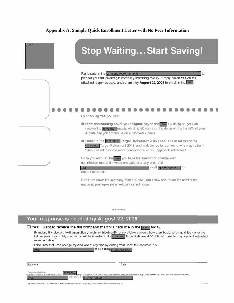
Appendix A: Sample Quick Enro

34

ollment Lettter with Noo Peer Informmation

Appendiix B: Samplle Quick En

35

nrollment Leetter with PPeer Information

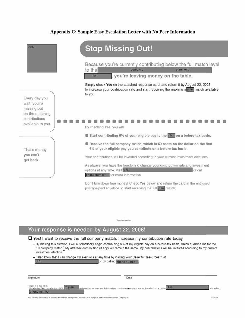
Appendixx C: Samplee Easy Esca

36

alation Letteer with No PPeer Informmation

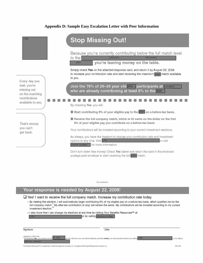
Appenddix D: Sampple Easy Esc

37

calation Lettter with Peeer Informaation

Table I: Features of the Four Subpopulations in the Experiment This table summarizes the key features of the four subpopulations that were targeted in the field experiment. Quick Enrollment recipients Easy Escalation recipients 0% contribution

rate default 6% contribution

rate default 0% contribution

rate default 6% contribution

rate default Union membership

Yes No Yes No

Savings plan enrollment mechanism

Opt-in Opt-out (automatic enrollment)

Opt-in Opt-out (automatic enrollment)

Savings plan participation status prior to experiment

Non-participant Non-participant Participant Participant

Savings plan contribution rate prior to experiment

0% 0% Less than 6% and less than their 401(k)

match threshold

Less than 6% (which is their 401(k) match

threshold)

Savings plan decision prior to experiment

Passively accepted default 

Actively opted out of plan 

Actively chose contribution rate 

Actively chose contribution rate 

Table II: Employer Match Formulas This table describes the employer match formulas that applied to different groups of employees at the firm.

Match formula for before-tax contributions

Number of employees included in the mailing with this match

Union Non-union Match A 100% on the first 1% of pay contributed

50% on the next 5% of pay contributed 0 3,158

Match B The minimum of $325 or 50% on the first 2% of pay contributed

126 0

Match C 100% on the first 2% of pay contributed 50% on the next 2% of pay contributed 25% on the next 4% of pay contributed

1,114 0

Match D 100% on the first 2% of pay contributed 50% on the next 2% of pay contributed 25% on the next 2% of pay contributed

261 0

Match E 50% on the first 4% of pay contributed 135 0

Match F 50% on the first 6% of pay contributed 149 0

Match G† None 0 0 † This group was not included in the intervention.

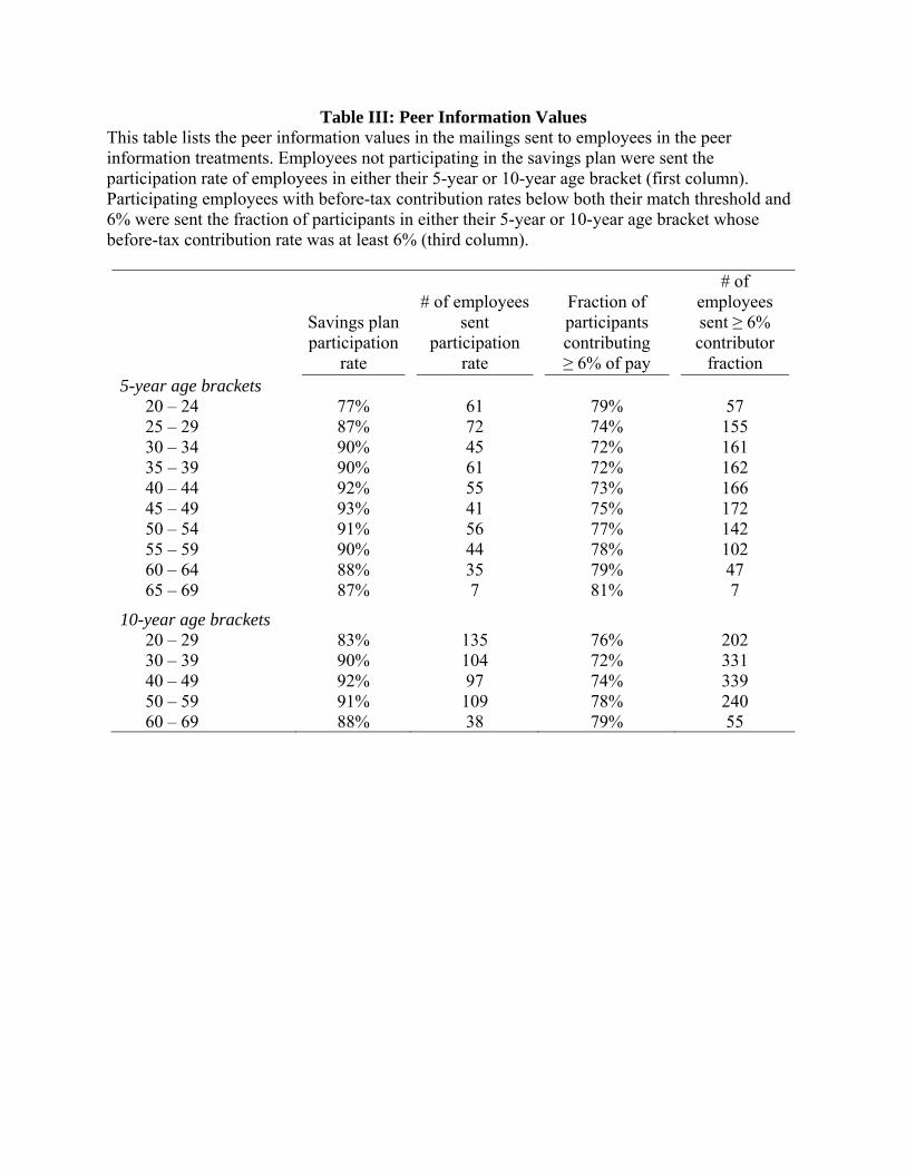
Table III: Peer Information Values This table lists the peer information values in the mailings sent to employees in the peer information treatments. Employees not participating in the savings plan were sent the participation rate of employees in either their 5-year or 10-year age bracket (first column). Participating employees with before-tax contribution rates below both their match threshold and 6% were sent the fraction of participants in either their 5-year or 10-year age bracket whose before-tax contribution rate was at least 6% (third column).

Savings plan participation

rate

# of employees sent

participation rate

Fraction of participants contributing ≥ 6% of pay

# of employees sent ≥ 6% contributor

fraction 5-year age brackets

20 – 24 77% 61 79% 57 25 – 29 87% 72 74% 155 30 – 34 90% 45 72% 161 35 – 39 90% 61 72% 162 40 – 44 92% 55 73% 166 45 – 49 93% 41 75% 172 50 – 54 91% 56 77% 142 55 – 59 90% 44 78% 102 60 – 64 88% 35 79% 47 65 – 69 87% 7 81% 7

10-year age brackets 20 – 29 83% 135 76% 202 30 – 39 90% 104 72% 331 40 – 49 92% 97 74% 339 50 – 59 91% 109 78% 240 60 – 69 88% 38 79% 55

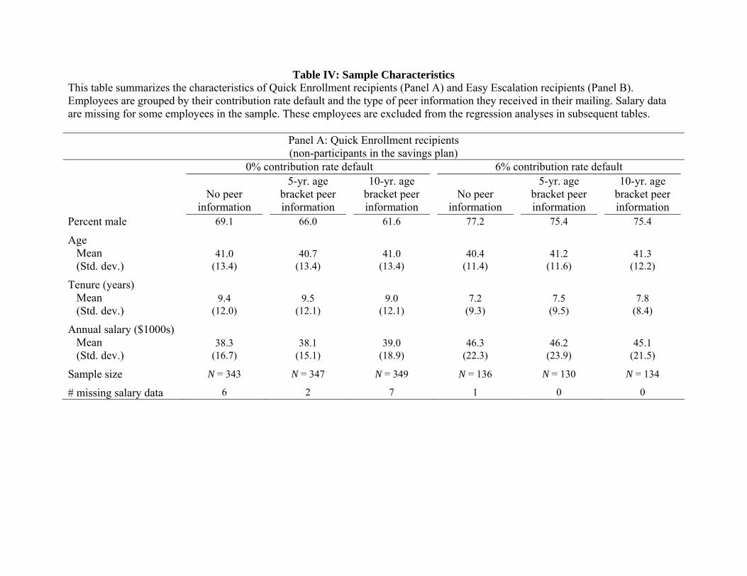
Table IV: Sample Characteristics This table summarizes the characteristics of Quick Enrollment recipients (Panel A) and Easy Escalation recipients (Panel B). Employees are grouped by their contribution rate default and the type of peer information they received in their mailing. Salary data are missing for some employees in the sample. These employees are excluded from the regression analyses in subsequent tables.

Panel A: Quick Enrollment recipients (non-participants in the savings plan)

0% contribution rate default 6% contribution rate default

No peer information

5-yr. age bracket peer information

10-yr. age bracket peer information

No peer information

5-yr. age bracket peer information

10-yr. age bracket peer information

Percent male 69.1 66.0 61.6 77.2 75.4 75.4

Age Mean 41.0 40.7 41.0 40.4 41.2 41.3 (Std. dev.) (13.4) (13.4) (13.4) (11.4) (11.6) (12.2)

Tenure (years) Mean 9.4 9.5 9.0 7.2 7.5 7.8 (Std. dev.) (12.0) (12.1) (12.1) (9.3) (9.5) (8.4)

Annual salary ($1000s) Mean 38.3 38.1 39.0 46.3 46.2 45.1 (Std. dev.) (16.7) (15.1) (18.9) (22.3) (23.9) (21.5)

Sample size N = 343 N = 347 N = 349 N = 136 N = 130 N = 134

# missing salary data 6 2 7 1 0 0

Panel B: Easy Escalation recipients (plan participants with initial before-tax contribution rate < min{match threshold, 6%})

0% contribution rate default 6% contribution rate default

No peer information

5-yr. age bracket peer information

10-yr. age bracket peer information

No peer information

5-yr. age bracket peer information

10-yr. age bracket peer information

Percent male 61.3 51.8 52.0 67.7 67.6 69.5

Age Mean 39.9 40.8 41.1 41.8 42.0 42.0 (Std. dev.) (11.7) (11.8) (11.9) (10.6) (10.7) (10.5)

Tenure (years) Mean 11.4 10.6 10.5 10.7 10.5 11.1 (Std. dev.) (10.1) (9.8) (10.6) (10.2) (9.6) (9.9)

Annual salary ($1000s) Mean 43.8 42.0 41.1 57.4 56.1 58.3 (Std. dev.) (16.2) (13.3) (14.2) (30.3) (24.8) (28.3)

Before-tax contrib. rate Mean 2.5 2.5 2.6 1.9 1.8 1.8 (Std. dev.) (1.8) (1.8) (1.8) (1.7) (1.8) (1.8)

Sample size N = 235 N = 255 N = 256 N = 931 N = 916 N = 911

# missing salary data 0 0 0 0 2 3

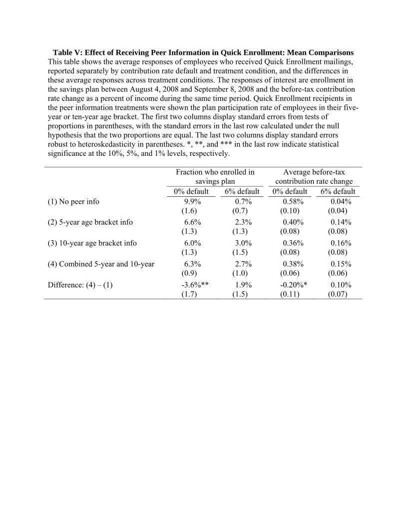
Table V: Effect of Receiving Peer Information in Quick Enrollment: Mean Comparisons This table shows the average responses of employees who received Quick Enrollment mailings, reported separately by contribution rate default and treatment condition, and the differences in these average responses across treatment conditions. The responses of interest are enrollment in the savings plan between August 4, 2008 and September 8, 2008 and the before-tax contribution rate change as a percent of income during the same time period. Quick Enrollment recipients in the peer information treatments were shown the plan participation rate of employees in their five-year or ten-year age bracket. The first two columns display standard errors from tests of proportions in parentheses, with the standard errors in the last row calculated under the null hypothesis that the two proportions are equal. The last two columns display standard errors robust to heteroskedasticity in parentheses. *, **, and *** in the last row indicate statistical significance at the 10%, 5%, and 1% levels, respectively. Fraction who enrolled in

savings plan Average before-tax

contribution rate change 0% default 6% default 0% default 6% default (1) No peer info 9.9%

(1.6) 0.7%

(0.7) 0.58%

(0.10) 0.04%

(0.04)

(2) 5-year age bracket info 6.6% (1.3)

2.3% (1.3)

0.40% (0.08)

0.14% (0.08)

(3) 10-year age bracket info 6.0% (1.3)

3.0% (1.5)

0.36% (0.08)

0.16% (0.08)

(4) Combined 5-year and 10-year 6.3% (0.9)

2.7% (1.0)

0.38% (0.06)

0.15% (0.06)

Difference: (4) – (1) -3.6%** (1.7)

1.9% (1.5)

-0.20%* (0.11)

0.10% (0.07)

Table VI: Effect of Receiving Peer Information in Quick Enrollment: Regression Analysis This table reports the results of ordinary least-squares regressions where the dependent variable is either a dummy for enrolling in the savings plan between August 4, 2008 and September 8, 2008 or the before-tax contribution rate change during the same time period. The sample is Quick Enrollment recipients who have a 0% contribution rate default (columns 1 and 3) or a 6% contribution rate default (columns 2 and 4). The linear spline in recipient age has knot points at 22.5, 27.5, 32.5, …, and 67.5. All regressions include a constant. Standard errors robust to heteroskedasticity are in parentheses. *, **, and *** indicate statistical significance at the 10%, 5%, and 1% levels, respectively. Dependent variable:

Enrolled in savings plan Dependent variable:

Before-tax contribution rate change 0% default 6% default 0% default 6% default Received peer info -0.040** 0.019 -0.221** 0.099 dummy (0.019) (0.014) (0.112) (0.078)

Male dummy -0.013 -0.031 -0.044 -0.154 (0.020) (0.021) (0.116) (0.113)

log(Tenure) -0.025*** -0.010 -0.146*** -0.054 (0.008) (0.006) (0.047) (0.035)

log(Salary) 0.007 0.038* 0.021 0.252* (0.021) (0.024) (0.129) (0.136)

Age spline Yes Yes Yes Yes

R2 0.033 0.048 0.029 0.052

Sample size N = 1,024 N = 399 N = 1,024 N = 399

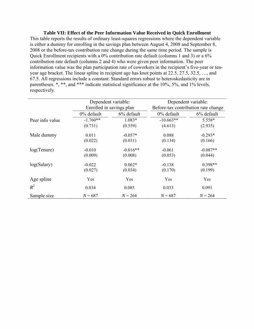
Table VII: Effect of the Peer Information Value Received in Quick Enrollment This table reports the results of ordinary least-squares regressions where the dependent variable is either a dummy for enrolling in the savings plan between August 4, 2008 and September 8, 2008 or the before-tax contribution rate change during the same time period. The sample is Quick Enrollment recipients with a 0% contribution rate default (columns 1 and 3) or a 6% contribution rate default (columns 2 and 4) who were given peer information. The peer information value was the plan participation rate of coworkers in the recipient’s five-year or ten-year age bracket. The linear spline in recipient age has knot points at 22.5, 27.5, 32.5, …, and 67.5. All regressions include a constant. Standard errors robust to heteroskedasticity are in parentheses. *, **, and *** indicate statistical significance at the 10%, 5%, and 1% levels, respectively. Dependent variable:

Enrolled in savings plan Dependent variable:

Before-tax contribution rate change 0% default 6% default 0% default 6% default Peer info value -1.760** 1.083* -10.663** 5.558* (0.731) (0.559) (4.613) (2.935)

Male dummy 0.011 -0.057* 0.088 -0.293* (0.022) (0.031) (0.134) (0.166)

log(Tenure) -0.010 -0.016** -0.061 -0.087** (0.009) (0.008) (0.053) (0.044)

log(Salary) -0.022 0.062* -0.138 0.398** (0.027) (0.034) (0.170) (0.199)

Age spline Yes Yes Yes Yes

R2 0.034 0.085 0.033 0.091

Sample size N = 687 N = 264 N = 687 N = 264

Table VIII: Effect of the Peer Information Value Received in Quick Enrollment: Sources of Identification

This table reports the peer information value coefficients from ordinary least-squares regressions analyzing employee responses to Quick Enrollment mailings. The coefficients in each cell come from separate regressions. The sample is recipients of Quick Enrollment mailings that included a peer information value equal to the savings plan participation rate of coworkers in either the recipient’s five-year or ten-year age bracket. Depending on the row, the sample is further restricted to employees with a 0% contribution rate default or a 6% contribution rate default. The dependent variable is either a dummy for enrolling in the savings plan between August 4, 2008 and September 8, 2008 or the before-tax contribution rate change during the same time period. The column headings indicate the source of variation used to identify the peer information value coefficient. All regressions include controls for gender, log tenure, log salary, and a constant, as in Table VII, as well as a linear spline in recipient age with knot points at 22.5, 27.5, 32.5, …, and 67.5. Additional controls for age are included as indicated in the bottom rows. Standard errors robust to heteroskedasticity are in parentheses. *, **, and *** indicate statistical significance at the 10%, 5%, and 1% levels, respectively.

Source of identification for the effect of the peer information value

Baseline (from Table

VII)

Differences in 5-year vs. 10-year peer

information values

Discontinuities around age

bracket boundariesDependent variable: Enrolled in savings plan

0% contribution rate default (N = 687) -1.760** -1.970** -0.736 (0.731) (0.816) (1.224)

6% contribution rate default (N = 264) 1.083* 1.490* 0.994 (0.559) (0.881) (1.025)

Dependent variable: Before-tax contribution rate change

0% contribution rate default (N = 687) -10.663** -11.784** -5.237 (4.613) (5.073) (7.611)

6% contribution rate default (N = 264) 5.558* 9.038* 3.180 (2.935) (5.261) (3.860)

Age controls Age spline Yes Yes Yes 5-yr. age group dummies No Yes No Rec’d 10-year age group info dummy No No Yes Age spline × rec’d 10-year age group info No No Yes

Table IX: Effect of the Peer Information Value Received in Quick Enrollment: Robustness to Different Age Controls

This table reports the peer information value coefficients from ordinary least-squares regressions analyzing employee responses to Quick Enrollment mailings. The estimated coefficients in each cell come from separate regressions. The sample is recipients of Quick Enrollment mailings that included a peer information value equal to the savings plan participation rate of coworkers in either the recipient’s five-year or ten-year age bracket. The sample is further restricted to those with a 0% contribution rate default (columns 1 and 3) or a 6% contribution rate default (columns 2 and 4). The dependent variable is either a dummy for enrolling in the plan between August 4, 2008 and September 8, 2008 or the before-tax contribution rate change during the same time period. All regressions include controls for gender, log tenure, log salary, and a constant, as in Table VII. The regressions vary in how they control for recipient age: (1) a linear spline in age with knot points at 22.5, 27.5, 32.5, …, and 67.5 (every five years), which is the baseline; (2) a linear spline in age with knot points at 22.5, 25, 27.5, …, and 67.5 (every 2.5 years); (3) a linear spline in age with knot points every 5 years and dummies for the target date retirement fund offered, which is dependent on age; (4) a linear spline in age with knot points every five years and controls for the number of years the recipient is from the age group mean (linear and squared terms); or (5) a linear spline in age with knot points every five years and controls for the recipient’s percentile rank in the age group (linear and squared terms). Standard errors robust to heteroskedasticity are in parentheses. *, **, and *** indicate statistical significance at the 10%, 5%, and 1% levels, respectively.

Dependent variable:

Enrolled in savings plan

Dependent variable: Before-tax contribution

rate change Parameterization of age controls 0% default 6% default 0% default 6% default Age spline with knot points every 5 -1.760** 1.083* -10.663** 5.558* years (Baseline from Table VII) (0.731) (0.559) (4.613) (2.935)

Age spline with knot points every -1.736** 1.342** -10.520** 6.760** 2.5 years (0.734) (0.662) (4.636) (3.285)

Dummies for target date retirement -1.931*** 0.990* -11.665** 5.797* fund offered (0.723) (0.574) (4.558) (3.396)

Controls for years from age group -2.041** 0.890 -12.220** 5.111 mean (linear and squared) (0.797) (0.596) (4.994) (3.517)

Controls for percentile within age -1.757** 1.180* -10.438** 6.519* group (linear and squared) (0.748) (0.657) (4.673) (3.798)

Sample size N = 687 N = 264 N = 687 N = 264

Table X: Effect of Receiving Peer Information in Easy Escalation: Mean Comparisons This table shows the average responses of employees who received Easy Escalation mailings, reported separately by contribution rate default and treatment condition, and the differences in these average responses across treatment conditions. The responses of interest are increasing one’s before-tax contribution rate between August 4, 2008 and September 8, 2008 and the before-tax contribution rate change during the same time period. Easy Escalation recipients in the peer information treatments were shown the fraction of plan participants in their five-year or ten-year age bracket with before-tax contribution rates of at least 6%. The first two columns display standard errors from tests of proportions in parentheses, with the standard errors in the last row calculated under the null hypothesis that the two proportions are equal. The last two columns display standard errors robust to heteroskedasticity in parentheses. *, **, and *** in the last row indicate statistical significance at the 10%, 5%, and 1% levels, respectively. Fraction who increased

before-tax contribution rate Average before-tax

contribution rate change 0% default 6% default 0% default 6% default (1) No peer info 10.6%

(2.0) 8.2%

(0.9) 0.33%

(0.08) 0.26%

(0.04) (2) 5-year age bracket info 9.8%

(1.9) 7.8%

(0.9) 0.30%

(0.07) 0.29%

(0.05) (3) 10-year age bracket info 11.3%

(2.0) 8.8%

(0.9) 0.38%

(0.09) 0.40%

(0.07) (4) Combined 5-year and 10-year 10.6%

(1.4) 8.3%

(0.6) 0.34%

(0.06) 0.35%

(0.05) Difference: (4) – (1) -0.1%

(2.4) 0.1%

(1.1) 0.01%

(0.10) 0.08%

(0.06)

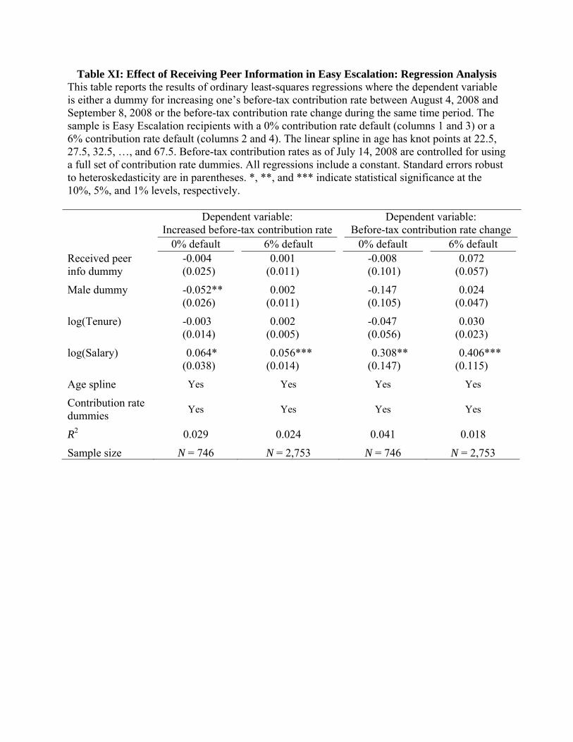
Table XI: Effect of Receiving Peer Information in Easy Escalation: Regression Analysis This table reports the results of ordinary least-squares regressions where the dependent variable is either a dummy for increasing one’s before-tax contribution rate between August 4, 2008 and September 8, 2008 or the before-tax contribution rate change during the same time period. The sample is Easy Escalation recipients with a 0% contribution rate default (columns 1 and 3) or a 6% contribution rate default (columns 2 and 4). The linear spline in age has knot points at 22.5, 27.5, 32.5, …, and 67.5. Before-tax contribution rates as of July 14, 2008 are controlled for using a full set of contribution rate dummies. All regressions include a constant. Standard errors robust to heteroskedasticity are in parentheses. *, **, and *** indicate statistical significance at the 10%, 5%, and 1% levels, respectively. Dependent variable:

Increased before-tax contribution rate Dependent variable:

Before-tax contribution rate change 0% default 6% default 0% default 6% default Received peer -0.004 0.001 -0.008 0.072 info dummy (0.025) (0.011) (0.101) (0.057)

Male dummy -0.052** 0.002 -0.147 0.024 (0.026) (0.011) (0.105) (0.047)

log(Tenure) -0.003 0.002 -0.047 0.030 (0.014) (0.005) (0.056) (0.023)

log(Salary) 0.064* 0.056*** 0.308** 0.406*** (0.038) (0.014) (0.147) (0.115)

Age spline Yes Yes Yes Yes

Contribution rate dummies

Yes Yes Yes Yes

R2 0.029 0.024 0.041 0.018

Sample size N = 746 N = 2,753 N = 746 N = 2,753

Table XII: Effect of the Peer Information Value Received in Easy Escalation This table reports the results of ordinary least-squares regressions where the dependent variable is either a dummy for increasing one’s before-tax contribution rate between August 4, 2008 and September 8, 2008 or the before-tax contribution rate change during the same time period. The sample is Easy Escalation recipients who were given peer information and have a 0% contribution rate default (columns 1 and 3) or a 6% contribution rate default (columns 2 and 4). The peer information value was the fraction of savings plan participants in the recipient’s five-year or ten-year age bracket with before-tax contribution rates of at least 6%. The linear spline in age has knot points at 22.5, 27.5, 32.5, …, and 67.5. Before-tax contribution rates as of July 14, 2008 are controlled for using a full set of contribution rate dummies. All regressions include a constant. Standard errors robust to heteroskedasticity are in parentheses. *, **, and *** indicate statistical significance at the 10%, 5%, and 1% levels, respectively. Dependent variable:

Increased before-tax contribution rateDependent variable:

Before-tax contribution rate change 0% default 6% default 0% default 6% default Peer info value 2.309 0.494 11.108 7.414* (1.901) (0.813) (7.085) (4.179)

Male dummy -0.035 -0.002 -0.050 0.014 (0.031) (0.014) (0.124) (0.062)

log(Tenure) 0.000 -0.002 -0.063 0.019 (0.017) (0.006) (0.069) (0.032)

log(Salary) 0.069 0.056*** 0.371* 0.487*** (0.055) (0.017) (0.215) (0.166)

Age spline Yes Yes Yes Yes

Contribution rate dummies

Yes Yes Yes Yes

R2 0.041 0.020 0.064 0.021

Sample size N = 511 N = 1,822 N = 511 N = 1,822

Table XIII: Effect of Receiving Peer Information in Quick Enrollment Among Employees with a 0% Contribution Default: Interaction with Relative Salary Within Firm and State

This table reports the results of ordinary least-squares regressions where the dependent variable is either a dummy for enrolling in the savings plan between August 4, 2008 and September 8, 2008 or the before-tax contribution rate change during the same time period. The sample in the left two columns is Quick Enrollment recipients who have a 0% contribution rate default. In the right two columns, this sample is further restricted to employees who received peer information. “Salary below median in firm and state” is a dummy for having a salary below the median salary among all active employees at the firm in the same state, including those not in the experiment. “Peer info value” is the plan participation rate of coworkers in the recipient’s five-year or ten-year age bracket. The linear spline in recipient age has knot points at 22.5, 27.5, 32.5, …, and 67.5. In the right two columns, all components of the age spline are also interacted with the salary below median dummy. All regressions include a constant. Standard errors robust to heteroskedasticity are in parentheses. *, **, and *** indicate statistical significance at the 10%, 5%, and 1% levels, respectively. Enrolled

in plan Contribution rate change

Enrolled in plan

Contribution rate change

Received peer info 0.007 0.042 dummy (0.018) (0.105)

Salary below -0.052* -0.291* median in firm and state × peer info

(0.028) (0.167)

Peer info value 0.984 5.988 (0.847) (5.112)

Salary below -2.844** -17.254** median in firm and state × peer value

(1.126) (7.025)

Salary below 0.079*** 0.457*** 3.923** 20.611** median in firm and state

(0.022) (0.132) (1.642) (9.140)

Male dummy -0.011 -0.035 0.014 0.108 (0.020) (0.118) (0.023) (0.139)

log(Tenure) -0.024*** -0.142*** -0.009 -0.055 (0.008) (0.047) (0.009) (0.054)

log(Salary) 0.021 0.100 -0.017 -0.108 (0.023) (0.137) (0.029) (0.178)

Age spline Yes Yes Yes Yes

Salary below med. × age spline

No No Yes Yes

R2 0.035 0.031 0.041 0.040

Sample size N = 1,024 N = 1,024 N = 687 N = 687

Table XIV: Effect of Receiving Peer Information in Quick Enrollment Among Employees with a 0% Contribution Default: Interaction with Salary Relative to Firm-Wide Median

This table reports the results of ordinary least-squares regressions where the dependent variable is either a dummy for enrolling in the savings plan between August 4, 2008 and September 8, 2008 or the before-tax contribution rate change during the same time period. The sample in the left two columns is Quick Enrollment recipients who have a 0% contribution rate default. In the right two columns, this sample is further restricted to employees who received peer information. “Salary below firm median” is a dummy for having a salary below the median salary among all active employees in the firm, including those not in the experiment. “Peer info value” is the plan participation rate of coworkers in the recipient’s five-year or ten-year age bracket. The linear spline in recipient age has knot points at 22.5, 27.5, 32.5, …, and 67.5. In the right two columns, all components of the age spline are also interacted with the salary below firm median dummy. All regressions include a constant. Standard errors robust to heteroskedasticity are in parentheses. *, **, and *** indicate statistical significance at the 10%, 5%, and 1% levels, respectively. Enrolled

in plan Contribution rate change

Enrolled in plan

Contribution rate change

Received peer info -0.025 -0.149 dummy (0.032) (0.192)

Salary below firm -0.019 -0.089 median × peer info (0.039) (0.230)

Peer info value -2.189 -13.142 (1.989) (11.911)

Salary below firm 0.458 2.647 median × peer value (2.129) (12.823)

Salary below firm 0.051 0.281 0.654 0.776 median (0.039) (0.232) (1.914) (10.943)

Male dummy -0.013 -0.045 0.013 0.100 (0.020) (0.117) (0.022) (0.137)

log(Tenure) -0.024*** -0.144*** -0.009 -0.054 (0.008) (0.047) (0.009) (0.054)

log(Salary) 0.028 0.141 -0.010 -0.069 (0.025) (0.153) (0.033) (0.206)

Age spline Yes Yes Yes Yes

Salary below firm med. × age spline

No No Yes Yes

R2 0.034 0.030 0.043 0.042

Sample size N = 1,024 N = 1,024 N = 687 N = 687

Table XV: Effect of Receiving Peer Information in Easy Escalation: Interaction with Before-Tax Contribution Rate Prior to the Experiment

This table reports the results of ordinary least-squares regressions where the dependent variable is either a dummy for increasing one’s before-tax contribution rate between August 4, 2008 and September 8, 2008 or the before-tax contribution rate change during the same time period. The sample is Easy Escalation recipients with a 0% contribution rate default (columns 1 and 3) or a 6% contribution rate default (columns 2 and 4). Before-tax contribution rates as of July 14, 2008 are controlled for using a full set of contribution rate dummies. The regressions also include the interaction between the dummy for receiving peer information and a dummy for having a before-tax contribution rate of 0%, 1%, or 2% (as opposed to 3%, 4%, or 5%). The linear spline in age has knot points at 22.5, 27.5, 32.5, …, and 67.5. All regressions include a constant. Standard errors robust to heteroskedasticity are in parentheses. *, **, and *** indicate statistical significance at the 10%, 5%, and 1% levels, respectively. Dependent variable:

Increased before-tax contribution rate Dependent variable:

Before-tax contribution rate change 0% default 6% default 0% default 6% default Received peer 0.038 -0.019 0.175* -0.041 info dummy (0.034) (0.021) (0.090) (0.063)

Cont. rate 0% to -0.087* 0.032 -0.378* 0.184* 2% × peer info (0.049) (0.024) (0.200) (0.107)

Male dummy -0.052** 0.002 -0.147 0.024 (0.026) (0.011) (0.105) (0.047)

log(Tenure) -0.003 0.001 -0.048 0.029 (0.014) (0.005) (0.057) (0.023)

log(Salary) 0.059 0.056*** 0.286* 0.406*** (0.038) (0.014) (0.147) (0.115)

Age spline Yes Yes Yes Yes

Contribution rate dummies

Yes Yes Yes Yes

R2 0.033 0.025 0.045 0.018

Sample size N = 746 N = 2,753 N = 746 N = 2,753