The effect of local taxes on firm performance: evidence ... · PDF fileHighlights This paper studies the effect of business property taxation on a wide range of ﬁ rm-level outcomes,

Highlights

This paper studies the effect of business property taxation on a wide range of fi rm-level outcomes, using a panel data of Italian manufacturing fi rms over the period 2001-2010.

We exploit a pairwise spatial differenced generalized method of moments estimator along with the exogenous variation in local taxes generated by the political alignment of each local government with the central one.

Our estimates show that property taxation exerts a negative and statistically signifi cant impact on employment, capital, TFP and sales.

Back-of-the-envelope calculations suggest that the observed average increase in business property taxation between two consecutive years (0.05 percentage points) induces contractions in employment and capital, by about 0.5 workers and 8150 euros, respectively.

The effect of local taxes

on firm performance:

evidence from geo referenced data

No 2016-03 – FebruaryWorking Paper

Federico Belotti, Edoardo di Porto & Gianluca Santoni

CEPII Working Paper The effect of local taxes on fi rm performance

Abstract

This paper investigates the impact of business property taxation on fi rms' performance using a panel of italian manufacturing fi rms. To account for endogeneity in local taxation, we exploit a pairwise spatial differenced generalized method of moments estimator. As well as providing robust inference, we also improve on existing work by exploiting the exogenous variation in local taxes generated by the political alignment of each local government with the central one. We fi nd that property taxation exerts a negative impact on fi rms' employment, capital and sales to such an extent as to signifi cantly affect total factor productivity.

Keywords

Local taxation, Endogeneity, Spatial differencing, Two-way clustering.

JEL

H22, H71, R38.

CEPII (Centre d’Etudes Prospectives et d’Informations Internationales) is a French institute dedicated to producing independent, policy-oriented economic research helpful to understand the international economic environment and challenges in the areas of trade policy, competitiveness, macroeconomics, international fi nance and growth.

CEPII Working PaperContributing to research in international economics

© CEPII, PARIS, 2016

All rights reserved. Opinions expressed in this publication are those of the author(s) alone.

Editorial Director:Sébastien Jean

Production: Laure Boivin

No ISSN: 1293-2574

CEPII113, rue de Grenelle75007 Paris+33 1 53 68 55 00

www.cepii.frPress contact: [email protected]

Working Paper

CEPII Working Paper The effect of local taxes on firm performance

The effect of local taxes on firm performance: evidence from geo referenced data1

Federico Belotti∗ Edoardo Di Porto† Gianluca Santoni‡

1We thank participants at the VI Italian Congress of Econometrics and Empirical Economics and the XXVISIEP Scientific Meeting, CSEF seminar participants at the University of Naples Federico II and UCFS seminarparticipants at University of Uppsala for useful discussions. We particularly thanks Tullio Jappelli, FrancescoDrago, Marco Pagano, Luigi Benfratello, Alessandro Sembenelli, Mario Padula, Emilio Calvano, Salvatore Morelli,Andrea Piano Mortari, Alex Solis, Eva Mork, Henry Ohlsson, Matz Dhalberg, Federico Revelli, Sonia Paty, GillesDuranton, Laurent Gobillon, for their critics and comments. All remaining errors are ours.∗CEIS, University of Rome Tor Vergata, [email protected]†University of Naples Federico II, CSEF and UCFS Uppsala University, [email protected]‡CEPII,[email protected]

3

mailto:[email protected]




1. Introduction

The property tax has long been one of the main source of financing at the local government

level. The new literature view about its economic incidence argues that it exerts distortionary

effects on the use of capital at local level (Zodrow, 2001). The empirical literature on the

economic effects of this widely used tax and, in general, of local taxation is extensive.2 Despite

this attention, the estimation of its impact is fraught with uncertainty and it is still one of the

more debated issues in public finance.

Recently, Duranton et al. (2011) point out three main sources of this uncertainty. First, it

may arise from the fact that many of the site’s characteristics affecting the firm’s choice on

where to localize its plants are unobservable by the analyst, and likely correlated with both

firm’s characteristics and local taxation. Second, a reverse causality may arise due to the likely

correlation between firm decisions and many aspects of the tax system itself. Third, a relevant

source of bias is likely provided by the presence of firm-specific unobserved heterogeneity. By

exploiting firm level panel data in which firms are geo-localized through postcodes, the authors

address the aforementioned issues by using spatial and time differencing data transformations

together with instrumental variables. They suggest without a formal statistical test that, by

conditioning out site-specific unobserved heterogeneity, spatial differencing is the key to make

plausible the exclusion restriction associated with their identification strategy. They provide

suggestive evidence that an increase in the property tax rate leads to substantial reductions

in firms employment (i.e., a growth slow-down effect) and no evidence of selection due to

property taxation.3

In this paper, we revisit the strategy of Duranton et al. (2011) to estimate the impact of

business property taxation on firms performance. As well as providing general guidance to

those attempting a similar appealing strategy, we extend their work in different directions.

First, we exploit a geo-coded panel of italian manufacturing firms for the period 2001-2010

that, taking into account both administrative boundaries and accurate firms’ geographical

coordinates, reduces the bias due to a suboptimal firms georeferencing, as is the case with

2For a review of the literature on the economics of property tax see Mieszkowski and Zodrow (1989). For acomprehensive review of the effect of local taxation on resource allocation, see Bartik (1991). For more recentreferences on empirical local public finance, see Revelli (2015).3Local taxation represents a cost that can be reduced by moving production facilities to a new location charac-terized by a lower tax rate. However, if a firm choose to relocate, then it will face the cost of moving its assetsto the new location. Clearly, if relocation costs are higher than local taxation costs regardless of the location, afirm will linger in its original location suffering what Duranton et al. (2011) define as slow-down effect; while if itrelocates this will cause the so-called “selection” effect. Indeed, movers are likely to be the most efficient firmsand will tend to relocate in low tax rate jurisdictions. We provide a simple test of selection-into-treatment findingno significant evidence of selection effect in our sample (see Appendix 8) for details.

4


postcodes. This enables to pair firms based on their actual distance in a very refined way

and to apply spatial differentiation to all firms located in different municipalities and distant

less then a certain threshold.4 Second, we provide a novel identification strategy for the

impact of local taxation based on the political alignment between municipal governments and

the central one.5 This instrumenting strategy identifies the local average treatment effect

for the subpopulation of neighbouring firms located in distinct municipalities characterized by

different political alignment. Third, even though Duranton et al. (2011) provide a standard

errors correction to explicitly control for the cross-sectional dependence induced by the spatial

difference transformation, the authors correctly acknowledge that their inference is not robust

to heteroskedasticity, serial correlation or other forms of cross-sectional dependence. Since

we find strong evidence of heteroskedasticity and serial correlation in the data, we base our

inference on efficient generalized method of moments estimates and two-way clustered standard

errors (Cameron and Miller, 2015). Fourth, even thought employment can be considered a good

indicator of firm growth from a short run perspective, oversizing firms may be inefficient and

are likely to face a productivity slow-down in the medium run (Guiso and Rustichini, 2010).

Furthermore, firms may improve their performances without increasing their labor force but

just re-organizing or innovating their production process. In order to provide a more complete

picture of the impact of local taxation, we consider a wider range of firms’ outcomes by looking

not only at employment but also at capital, sales and total factor productivity (TFP).6 Finally,

since agglomeration forces are likely to generate rents that local governors can exploit by

raising taxation (Baldwin and Krugman, 2004), we split our sample according to the degree of

urbanization at a local labor system (LLS) level in order to provide a test for the presence of

agglomeration rents.7

The main empirical findings are as follows. We show that the spatial differencing is indeed

the key to make our instrumenting strategy plausible, this evidence is supported by appropri-

ate over-identification tests. Furthermore, we show that clustering is the key to provide a

meaningful inference. We find that the semi-elasticities to local taxation are always negative

and significant, specifically about -0.3 for capital, -0.11 for employment, -0.14 for TFP and

-0.21 for sales. Back-of-the-envelope calculations suggest that the observed average increase

in business property taxation between two consecutive years, which in our sample is found to

be about 0.05 percentage points, induces economically plausible contractions in employment

and capital, by about 0.5 workers and 8150 euros, respectively. These results are robust to

4We provide a discussion of the issues of georeferencing firms based on postcodes in Section 3.5From now on, we refer to the political alignment of municipal governments with the central government just aspolitical alignment.6See Section 4.1 for some theoretical arguments that could clarify our line of reasoning.7We find a rather strong evidence that denser italian jurisdictions set higher tax rates. See Section 3 for details.

5


a number of different specifications and instrumenting strategies. Our test for the Baldwin-

Krugman agglomeration rents hypothesis confirms that, in high density areas, the negative

effect of taxation is diluted by agglomeration economic forces.

2. Italian Institutional Framework

Italy is organized as a three-tier system of sub-national governments, whose layers are re-

spectively regions, provinces and municipalities. The 8,100 municipalities are the smallest

administrative units with delegated fiscal power.8 This makes them an ideal environment to

test for spatial interactions and informational externalities which, intuitively, are more likely to

arise the smaller is the scale of the units under observation. Municipalities are multi purpose

governments, their major functions being registry, waste disposal, urban planning, illumination,

road maintenance, local transports, social aid, child care, primary schooling, and assistance

to the elderly. Expenditures are financed by grants (roughly by 45 percent), own taxes (30

percent) and other own revenues (such as tariffs, fees and penalties). Municipal taxes are

manifold, but the major one is undoubtedly the local property tax, which accounts for more

than half of total tax revenues; other important funding sources are the taxes on solid waste

management, the latter works fairly as a tariff rather than as a tax covering a given share of

waste.

Our analysis focuses on local property taxation, which represents the main leverage of the

municipal fiscal power. This tax has a rate spanning from 0.4 to 0.7 percentage points of

the tax base (which is a function of property’s cadastral values and squared meters) and is

differentiated between residential and business properties. In particular, we focus on property

taxation concerning business properties. In this case, cadastral values are set taking into

account also bolted heavy machineries (e.g., blast-furnaces, hydraulic presses, etc.) making

this tax a classical tax on capital (See Zodrow, 2001, on this point).

The ability to set business property tax rates was probably the only expression of municipal fiscal

powers in the period under observation since alternative forms of taxing powers, namely the

ability to manoeuvre the surcharge on national personal income tax (IRPEF), were hampered

by national legislation. Finally, since residential property tax has de facto been abolished in

2008 and proposals for a future revision of municipal financing structure point to business

properties as the principal source for local taxation, our analysis assumes even more relevance.

At regional level another important tax is levied, the business tax (IRAP), a proportional tax on

value added mainly financing the italian national health system. It is worth noting that while

8On average each municipality lays on an area of 14 square miles.

6


this tax was the same at national level until 2008, some regions (Abruzzo, Campania, Lazio,

Molise and Sicilia) increased the tax rate in order to adjust their fiscal budget starting from

2009.

3. Data and summary statistics

In order to implement the methodology described in Section 4, we build our data set merging

information from several sources. The resulting sample is an unbalanced panel containing

balance sheet information for a sample of italian manufacturing firms for the period 2001-

2010, as well as information on firms’ geographical coordinates (latitude and longitude). It

is worth noting that such refined data helps to reduce the bias due to inaccurate firm geo-

referentiation, as is the case when firms are referenced using zoning system centroids (e.g.,

centroids of zip-codes, postcodes, etc.).

3.1. The Modifiable Unit Area Problem

The negative effect of the zoning system on statistical results is known as modifiable area unit

problem (MAUP). The bias induced by scale and shape effects is minimized if the units are:

identical (shape, size and neighboring structure) and spatially independent (Arbia, 1989). Two

very difficult prerequisites to meet in practice.9 Figure 1 reports a graphical explanation of

this issue related to our purposes. The example is based on four jurisdictions (e.g., munici-

palities, regions, etc.) and five firms: in the left plot each firm is paired across jurisdictions

by their Euclidean distance using accurate geographical coordinates; in the right plot each ju-

risdiction is divided into smaller areas (e.g., postcodes) and firm location is determined using

the area’s centroid. Even assuming a fairly homogenous size distribution, it is evident how

the zoning scheme affects the distance between firms. If the objective is to pair firms based

on their distance, this will clearly affect the pairing process and, as a consequence, the final

estimation sample. Actually postcode areas are highly heterogeneous in both size and borders

shape, implying that a postcode-based pairing process may be seriously affected compared to

a coordinates-based pairing process.

We focus our analysis to the smallest administrative italian entity, the municipality, passing

over any compound treatment irrelevancy (Keele and Titiunik, 2014). For each municipality

and year, we have information on the population density and on the business property tax9Briant et al. (2010) show that the size distribution of geographical units affects statistical results, especiallywhen the dependent variable is not aggregated at the same level. However, their results using french employmentareas also indicate that the bias induced by the MAUP is of second order with respect to model miss-specification.On the other hand, Menon (2012) exploit MAUP to evaluate the significance of economic concentration in UStravel regions using randomly generated spatial units as control.

7


rate imposed by the local authority. We further merge information on the results of local and

national elections, which we exploit to build our identification strategy (see Section 4.2.1).

3.2. Firm level data

Firm level data are obtained from the AIDA dataset, provided by Bureau Van Dijk10. We

use the AIDA Top version which contains information on companies with a turnover above

1,5 millions of euro. This implies that small and medium enterprises are likely to be under-

represented with respect to bigger firms. For example, in 2010 manufacturing firms with less

than 50 employees account for 28 percent of total turnover in our data, against the 32 percent

reported in the aggregate national statistics. The complete dataset contains the exact (geo-

referenced) location along with balance sheet information of over 275,000 italian enterprises, in

this version financial accounts of subsidiaries are not consolidated in the corporate one. Firms

are classified according to the main sector of activity (NACE, rev 2), we focus our attention

on the manufacturing sector, namely to firms ranging from 2-digit NACE10 to NACE33. After

discarding observations with missing data, we end up with an unbalanced panel of 21,603

manufacturing firms for the period 2001-2010.11 Looking at the sectorial composition, our

data seems to give a fairly good representation of italian’s aggregate production structure,

the share of employment, turnover and value added by industry (2-digits) correlates above

90 percent with the shares computed using manufacturing firms population from the italian

national statistical institute (ISTAT). Moreover, if we look at the sector, province and year

shares the distribution of firms in our data correlates at 82 percent with the official statistics

on the overall number of active firms.12

Since we only observe firms, not plants, and we are interested in measuring the impact of

the local business property tax rate on different firm’s outcomes, multi-plant enterprisers may

be a cause of concern. Noteworthy, the phenomenon of multi-plant firms in Italy is relatively

modest, in 2010, according to ISTAT more than 90 percent of manufacturing firms have

only one production plant. Another potential issue is related to firms relocation, that we do

not observe directly in the data. Tracking movement of firms across the italian territory is

not straightforward, we can only infer the order of magnitude of the phenomenon from the

Chambers of Commerce, that maintains the register of all active enterprisers by Province

(NUTS3). In 2010, the first year for which the information is available, the Chambers of

Commerce recorded around 411,000 new economic entities, but among them only about 50

10http://www.bvdep.com.11We also drop observations with implausible negative values for sales and value added, and keep only firms thatstay in the sample for at least three years.12Those data are provided by the National Chamber of Commerce, Unioncamere.

8

http://www.bvdep.com


percent (213,000) were “true” new born firms, the remaining registration updates were due to

merge and acquisitions, changes in the juridical status and relocations.13 Considering that the

stock of active firms in 2010 was over 6 million enterprises, such changes, and among them

relocation, involved around 3.2 percent of the total.14

An advantage of our dataset is that we can test the effect of the local taxation on employment,

but we can also evaluate the effect on firms sales and TFP, extending previous results to other

aspect of firm’s behavior. We consider a value added TFP using the Levinsohn and Petrin

(2003) semi-parametric approach, controlling for unobservable shocks through intermediary

and energy inputs. Since book values for value added, fixed assets and intermediary inputs are

in nominal terms we use OECD industry specific deflators. Looking at the TFP is particularly

interesting given the fact that the business property tax considered here applies to production

building and, as such, it can be seen as a tax on fixed capital (see next section for a detailed

description of the property tax).

Table 1 reports the descriptive statistics for the overall analysis sample, as well as by level

of business property tax. Panel A provides descriptives for the considered outcome variables

showing that there is a negative correlation between three of these outcomes, namely number

of workers, capital and sales, and the property tax rate. For example, manufacturing firms

located in a municipality in which the tax rate is less than 5 percent have, on average, 30

percent more workers and capital and about 45 percent more sales than firms located in

municipality with highest tax rate. Panel B lists the observed firm’s characteristics and shows

that the average firm is 20 years old and that most of the firms in the analysis sample, about

87 percent, are located in northern regions, about 9 percent in central regions and only less

than 5 percent in southern regions. This unbalanced geographical distribution well reflects the

unequal development of the manufacturing industry in Italy. The last panel of Table 1 reports

summary statistics on the instrument. About 55 percent of the firms are located in a political

aligned municipality, 43 percent are located in a center-right aligned jurisdiction and about 12

percent in a center-left aligned jurisdiction. Interestingly, the percentage of firms located in a

political aligned municipality decreases when business property tax rate increases. This is an

evidence of the first-stage mechanism at work, something we discuss further in Section 4.2.1.

13Mayer et al. (2015) study the impact of a French enterprise zone program on establishment location decisionsand on labor market outcomes. They show that conditional on locating in a municipality that hosts a ZFU, thepolicy has a positive and sizeable impact on the probability to locate in the ZFU part rather than in the non-ZFUpart of municipalities. However, the impact is highly heterogeneous across zones. Most importantly and in linewith our assumptions, they show that this positive effect is entirely due to within-municipality diversion effects.They do not find any relocation effect across municipalities.14These figures refer to the whole economy, we do not have detailed information on the manufacturing sector.

9


3.3. Local taxation

Data on the local business property tax are from the italian Minister of Economics and Fi-

nances. The business property tax rate is defined independently by each municipality and, as

is true for many developed countries, represents one of the main source of financing for local

administrations: in 2010 around 45 percent of total tax revenues was represented by property

tax revenues. The effective tax burden results from the application of the effective rate to

the property rent. The rent is proportional to the size of the building and the land appraisal,

the latter is based on census areas, providing that in each municipality there may be several

census areas.15 This may be a cause of concern for our identification strategy. Interestingly,

the first introduction of land appraisal in Italy dates back to 1939.16 Since their introduction,

land values have been revised only once in 1990. Given that our period of interest is 2001-2010

and that we consider only firms within a range of less than 3 km, land values heterogeneity

should be completely captured by firms fixed-effects.

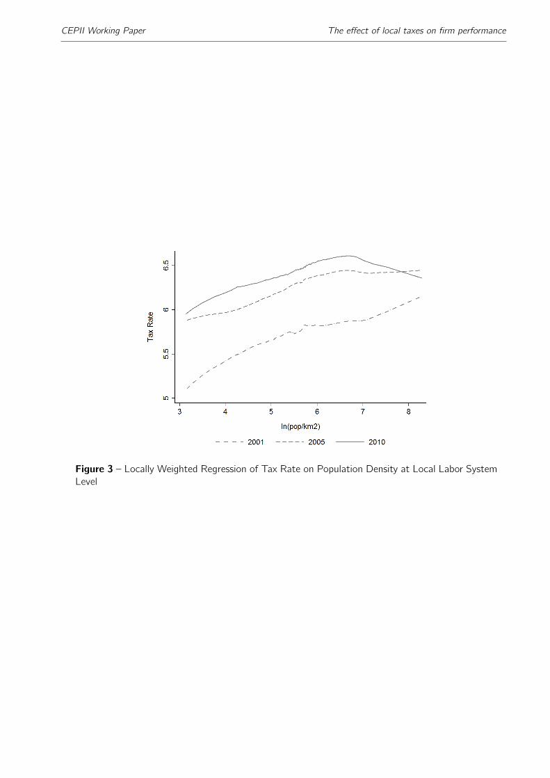
Figure 2 reports the geographical distribution of the business property tax rate. As can be

seen the imposed rate spread from 0.4 to 0.7 percent and, interestingly, there are no clear

cut geographical patterns. Furthermore, as we show in Figure 3, denser italian LLS include

municipalities characterized by higher tax rates, supporting the agglomeration rents hypothesis

suggested by Baldwin and Krugman (2004). We can also notice that, over time, the data

shows a generalized convergence of the effective tax rate to the highest level. Nonetheless, its

conditional distribution on LLS population density remains almost unchanged.

4. Empirical Strategy

4.1. The effect of business property tax on firm performance: expected results

Following previous literature, we assume that relocation expenses exceed the cost of taxation.17

Within this scenario, we expect business property tax to cause a growth slow-down not only in

employment but also across other dimensions.

Let us assume that there are two factors of production, capital and labour. Since it increases

input prices, an increase in business property tax should directly and negatively affect capital.

Providing that there is imperfect substitutability between the two factors, a credible assumption

15Note that census areas do not spread across multiple municipalities.16Law number 1249, 11th August 1939.17We cannot directly control for relocation effect due to data limitations; however, relocation is a relatively rareevent for italian manufacturing firms and does not appear to jeopardize our empirical strategy. We investigatethe effect of firm location in Appendix 8 by exploring the share of new born firms by municipality.

10


in the manufacturing sector, the effect of such tax on employment should be negative but lower

than the one on capital.

From a general equilibrium perspective, with two sectors, say manufacturing and services, a

prediction of this effect is way more difficult. In this case, an increase in the business property

tax rate is likely to determine an increase in the cost of capital for the more capital intensive

sector. This will, in turn, lead to an increase of the capital intensive products’ prices, thus

decreasing their relative demand and inducing a negative effect on sales. Firms operating in

the capital intensive sector will then try to exploit labour rather than capital, hence the effect

of business property tax on employment will depend on the degree of substitutability between

the two inputs, on the relative demand for labour by the two sectors and on the availability

of this latter input in the local labour market. As a result, the effect of business property tax

on employment is ambiguous and an empirical test is needed. This uncertainty sharpens if

we assume that the labour input is differently supplied in different local labour markets, e.g.

the labour input is more available and heterogenous within denser local labour markets. In

this setting, imperfect inputs substitutability could induce an unbalanced and inefficient re-

organization of production, thus making particularly appealing a test on the effect of local

taxation on TFP. If the effect of property tax on employment is positive, then re-organization

of the production structure is feasible for the capital intensive sector and TFP should not be

influenced at all. On the other hand, if the effect is negative, we expect TFP to be negatively

affected by an increase in taxation.

4.2. Econometric strategy

We are interested in estimating the impact of the business property tax rate on the aforemen-

tioned set of firm’s outcomes. The structural model of interest can be expressed as follows

yit = β1rat + β2ait + β3a2it + αi + δa + ψzt + θzt + εit , (1)

where yit is the log outcome of firm i at time t, rat is the business property tax rate in

municipality a, ait and a2it represent a second order polynomial of the firm’s age, αi is a firm

fixed-effect which captures the impact of unobservable time-invariant firm characteristics, δais a municipality fixed-effect capturing the impact of unobservable time-invariant municipality

characteristics, ψzt is a source of time-varying heterogeneity for location z , defined at a finer

spatial scale than a, that is local specific but does not vary continuously across space or, in

other words, does not spill over across the jurisdictions, θzt is a time-varying effect for location

11


z which, on the other hand, is assumed to vary continuously across space.18 Finally, εit is

the standard idiosyncratic error. The main parameter of interest in this model is β1 which

captures the average percentage change in the outcome of a firm for a unit increase in the

business property tax rate levied at municipal level, after controlling for firm’s age, unobserved

time-invariant heterogeneity and unobserved time-varying local heterogeneity.

One approach to estimating β = (β1, β2, β3) is to rule out αi and δa through a within-firm

transformation to get

yit = β1rat + β2ait + β3a2it + ψzt + θzt + εit , (2)

where yit = yit − yi with yi = 1Ti

∑Tit=1 yit . Model (2) will give consistent estimates only

if cov[(rat , ait , a2it), ψzt + θzt + εit ] = 0, a condition that is unlikely to hold since the local

effects are likely to be correlated across neighboring sites, implying that rat is likely to be

correlated with both ψzt and θzt . The standard way to deal with this correlation is to find a

suitable instrumenting strategy for the municipal tax rate. However, instruments for rat are

also likely to be correlated with unobserved time-varying local effects (ψzt and θzt) violating

the orthogonality condition.

An alternative to the instrumental variable approach is the spatial differentiation à la Duranton

et al. (2011), that is taking for each time t the difference between each reference firm and

any neighboring firm in the sample located at a distance less than d from the reference one.

Applying this transformation to model (2) gives

∆d yit = γ∆d rat + β2∆d ait + β3∆d a2it + ∆dψzt + ∆d θzt + ∆d εit , (3)

with ∆d being the spatial difference operator.

It is worth noting that, differently from Duranton et al. (2011), we only pair firms located in

different municipalities and distant less then d . This means that here we are exploiting only

neighbouring firms located across municipalities to identify the effects of taxation.19

Consistent estimates of β in model (3) can be obtained only if

cov[(∆d rat ,∆d ait ,∆d a2it),∆dψzt + ∆d θzt + ∆d εit ] = 0,

18It is worth noting that in the case in which firms do not change their location, the firm-fixed effects also controlfor unobserved time-invariant at local level.19Notice that including also neighbouring firms located in the same municipality does not improve the identificationof the effect of taxation, the variable of interest in this study, while clearly helps in improving the precision of theestimates of other exogenous firm-level covariates included in the model (here, ait and a2

it).

12


a condition that is likely to hold only if the spatial differentiation is performed using a (arbitrary

small) “optimal” distance d∗ and both ψzt and θzt vary continuously across space. Since ψztis not smoothed over space by assumption, ∆d

∗ψzt 6= 0 and the parameters of interest will not

be properly estimated by applying least squares to model (3).

It is worth to emphasize that the spatial difference transformation aims to remove any source of

smooth-over-space “local” spillovers potentially correlated with the independent variables in the

model and affecting firms’ performance. Thus, it does not mirror the practical estimation of the

treatment effect in a regression discontinuity design (RDD).20 Furthermore, RDD assumptions

are likely to be violated in our setting. Indeed, not only the treatment variable is endogenous,

but also the Stable Unit of Treatment Value Assumption (SUTVA) is likely to be violated due

to the presence of (unobserved) local spillovers that cross the boundaries (i.e. θzt) affecting

the performance of both treated and control groups.

For example, among other duties, italian municipalities spend their business property tax rev-

enues in urban planning. Suppose that one of this programs provides better conditions for local

businesses and improved logistics of goods and raw materials in an area that is close to the

border (e.g., quality roads or new infrastructures that reduce transport costs). In this case,

it is very likely that firms located near but beyond the border will benefit too. Thus, even

thought the treatment was exogenously assigned, the presence of these local spillovers creates

the conditions for a violation of the SUTVA in a regression discontinuity design at the border

(i.e., the spatial regression discontinuity design). This kind of local spillovers might also natu-

rally arise from fiscal competition among neighboring jurisdictions. For example, a jurisdiction

might want to create better conditions for local businesses by lowering the business tax rate.

In order to keep up with the competition, neighboring jurisdictions might reduce their own tax

rate too creating, in turn, better conditions for their local businesses.

These are examples of spatially smooth time-varying unobserved factors that can be easily

ruled out if the aforementioned spatial difference transformation is performed at the optimal

distance d∗. However, it is also possible to have other factors which may not spill over across

jurisdictions (i.e. ψzt) but are correlated with firm performances. An example could be the

(unobserved) quality of a locally provided public good that, due to institutional constraints,

affects only firms located in the specific jurisdiction in which the public good is effectively

provided, i.e. the efficiency of public kindergartens that release female labour supply in a local

labour market (Cascio, 2009). This kind of endogeneity cannot be easily removed through data

transformation, even if the spatial difference is performed at the optimal distance. Furthermore,

20See Imbens and Lemieux (2008) and Baum-Snow and Ferreira (2015) for a comprehensive reviews of RDD andRDD applications in urban economics, respectively.

13


since in practice one needs enough observations to estimate the model and the optimal distance

d∗ is unknown, spatial differentiation is likely to be applied at a non-optimal distance level,

implying that this strategy alone will be able to reduce but not eliminate all the endogeneity of

the municipal tax rate coming from θzt . This explain why we propose to exploit both spatial

differentiation and instrumental variables techniques to enhance the proper identification of the

β1 parameter.

More formally, a consistent IV estimator of β can be expressed in matrix notation as

βIV = (∆dXPZ∆dX)−1(∆dXPZ∆d y), (4)

with PZ = ∆dZ(∆dZ′,∆dZ)−1∆d Z

′and where ∆dX = (∆d rat ,∆d ait ,∆d a2

it) and ∆dZ are

the design and instruments matrices after within-firm projection and spatial differentiation,

respectively. As noted before, spatial differentiation induces a specific type of cross-sectional

dependence. In this case, the asymptotic variance of (4) can then be estimated by means of

the following sandwich type estimator

V (βIV ) = σ2ABA (5)

where A = (∆dXPZ∆dX)−1, B = ∆dX′PZ∆d∆d

′PZ∆dX, σ2 = ∆d ε′∆d ε

2N−tr(AB), ∆d ε = ∆d y −

∆dXβ, N =∑Pp=1 Tp, P the number of pairs, Tp the number of years that pair p appears in

the data and tr() is the trace operator.21 However, a key concern of this covariance matrix

estimator is that it completely ignores issues arising from serial correlation or any other type

of cross-sectional dependence of the errors. We applied the Wooldridge (2001) test for serial

correlation before any data transformation, i.e. model (1), and after the within-group/spatial

difference transformations, i.e. model (3) with d = (0.5km, 1km, 1.5km, 2km, 3km). In all

the cases the null hypothesis of no first-order autocorrelation was strongly rejected. Then,

following Cameron and Miller (2015), we based our statistical inference on the following two-

way cluster-robust covariance matrix estimator

V2way(βIV ) = V1(βIV ) + V2(βIV )− V12(βIV ), (6)

21Notice that ∆d , the spatial difference operator, is the (block) matrix that allows to spatially differentiate thewithin-firm transformed data (i.e., model (2)). For a formal representation of this matrix, see Appendix A, p.1040of Duranton et al. (2011).

14


where

V1(βIV ) = A∆dX′∆dZ(∆dZ

′∆dZ)−1W 1(∆dZ

′∆dZ)−1∆dXA, (7)

V2(βIV ) = A∆dX′∆d Z(∆dZ

′∆dZ)−1W 2(∆dZ

′∆dZ)−1∆dXA, (8)

V12(βIV ) = A∆dX′∆d Z(∆dZ

′∆dZ)−1W 12(∆d Z

′∆d Z)−1∆dXA, (9)

with

W 1 =

(P∑p=1

∆dZ′p∆d εp∆

d ε′p∆d Zp

), (10)

W 2 =

(T∑t=1

∆dZ′t∆d εt∆

d ε′t∆dZt

), (11)

W 12 =

(M∑m=1

∆d Z′m∆d εm∆d ε′m∆dZm

), (12)

with P the numbers of clusters at pair level, T the numbers of clusters at time (year) level and

M the numbers of clusters at pair-by-time level. Results from a set of preliminary Monte Carlo

simulations based on the data generating process in (1) show that, with critical value from

the T (J− 1) distribution with J = min(P, T ), the proposed two-way cluster-robust covariance

matrix estimator has the expected rejection rates in presence of multiplicative heteroskedasticity

and first-order serial correlation even in the case of few clusters (J = 10, 20, 30) with unequal

size.22 By using (6), we are making specific assumptions about the errors, that is observations

on the same pair in two different time periods are correlated (serial correlation) as well as

observations on two different pairs in the same time period (cross-sectional dependence). In

this case, and considering we are in a overidentified model (see Section 4.2.1), the classical IV

estimator is less efficient compared to the linear GMM estimator. Hence, our empirical analysis

is based on

βGMM = (∆dX∆dZWZ∆dZ′∆dX)−1(∆dX∆dZWZ∆dZ

′∆d y), (13)

where, for two-way clustered errors, the efficient two-step GMM estimator uses WZ = (W 1 +

W 2 − W 12)−1 in which ∆d εg for the generic cluster g is the IV residual, and

V2way(βGMM) = c(∆dX∆dZWZ∆dZ′∆dX)−1 (14)

22Since they are beyond the objective of this paper, for reasons of space these results are not included here butare available from the authors upon request.

15


where c = JJ−1

N−1N−k .

23

4.2.1. Identification strategy

Duranton et al. (2011) identification strategy is based on the municipal political color. The

rationale beyond this instrument is that, given their preference for redistribution, left-wing

administrators are more likely to set higher tax rates with respect to right-wing ones. How-

ever, this is likely to be correlated with unobserved local conditions such as inequality and/or

unemployment which, in turn, are correlated with firm-level outcomes. Alternatively, our in-

strumenting strategy is based on the political alignment of municipal government with the

central one, distinguishing whether the alignment is with right-wing or left-wing governments.

The relevance of our instrument comes from the fact that, as shown by Bracco et al. (2015),

municipalities sharing the same political color with the upper tier of government may exploit

up to 43 percent of extra grants compared to those that are not aligned, and more grants are

associated with lower local tax revenues. Stylized facts on business property tax rate differen-

tials between aligned and non aligned jurisdictions reported in Table 2 support this evidence,

showing that there is a statistically significant difference between the average tax rate set by

aligned and non aligned jurisdictions. Furthermore, Table 2 also suggests the presence of het-

erogeneity within the aligned jurisdictions, with municipalities aligned with a right-wing central

government systematically setting a lower tax rate.

As far as the validity of our instrument is concerned, even thought local conditions may affect

local voting behavior, the latter is marginal in determining the central government political color.

Indeed, non ideological “rational” citizens may exhibit different voting preferences conditional on

the type of election, e.g. foreign policy preferences may be important for national elections while

public transport and recycling may drive local voting behavior. This rules out the possibility that

local unobserved heterogeneity determining θzt and/or ψzt could also affect our instrument. As

in Duranton et al. (2011), to reflect the strength of the municipal aligned party at local level,

we weight the political alignment dummies with the share of the municipality’s population over

the reference electoral district population.24 The intuition behind such re-weighting is related

to the importance of distinguishing between municipalities like Rome or Milan and smaller

municipalities characterized by a different socio-economic framework as well as by a completely

different tax revenues and public spending profile. This interaction strengthens the relevance of

our instrumenting strategy leaving validity unchanged, as documented by the over-identifying

23GMM estimates have been obtained using the Baum and Schaffer (2012)’s ivreg2h Stata command on ap-propriately transformed data, that is by applying the efficient two-step linear GMM to model (3).24We use the electoral districts for the election of the National Parliament, districts borders are defined withinregions based on the electoral base the actual boundaries were established in 1993 law n. 227.

16


restriction tests (see Section 5).25 Since we find a clear evidence of heteroskedasticity driven

by the exogenous regressors (ait and a2it), we also use the method described in Lewbel (2012)

to supplement our instruments, improving both the identification of the tax-rate effect and the

efficiency of the GMM estimator.26

Finally, we also test an alternative identification strategy based on mandated compulsory ad-

ministration. When needed, italian law gives to the central government the power to remove

elected local officials and substitute them with external commissioners. This happens espe-

cially because of criminal organization infiltration but also when local budget administration

is under bailout. A similar instrument is used by Acconcia et al. (2014) to identify the effect

of public spending on the growth rate at provincial level (i.e., fiscal multiplier). We believe

that this could be considered a suitable instrument also for local business property tax rates,

since commissioners usually suspend investment projects and regulates financial flows into local

public works. Moreover, under bailout, they raise taxes in order to increase tax revenues.

5. Results

5.1. Baseline estimates

Table 3 reports our benchmark results for the four considered outcomes. We start by examining

Panel A and B of Table 3, which provide support for our empirical strategy. Panel A reports

estimates from the fixed-effects model in equation (2) showing why controlling only for time-

invariant firm unobserved heterogeneity is not enough: we obtain a positive and statistically

significant semi-elasticity of capital, something that is really hard to believe. We argue that

this result is likely driven by the endogeneity of local taxation, hence as discussed in Section

4.2, instrumenting the tax rate should solve the problem. Nonetheless, Panel B shows that

a fixed-effects GMM regression is still not sufficient to obtain plausible results, even thought

the coefficients of the first stage regression (reported in the first column of Table 4) do

have the expected sign and magnitude, supporting the hypothesized first-stage mechanism. A

possible explanation is that, as pointed out in Section 4.2, the instruments themselves might be

correlated with unobserved time-varying local effects, thus violating the orthogonality condition.

This is supported by the Hansen tests reported in Panel B of Table 3, which strongly reject

25It might be argued that the share of the municipality’s population over the reference electoral district may harmthe validity of the instrumenting strategy. We show that spatial differencing plays a key role in this regard, bycleaning out any source of local (spatially smooth) time-varying heterogeneity.26See Section 3.2 of Lewbel (2012) (pag. 73) for more details. In order to justify the use of heteroskedasticcovariance restrictions, we test for the presence of heteroskedaticity by using the LM test proposed by Juhl andSosa-Escudero (2014, see p.486) after model (2), strongly rejecting the null of homoskedasticity (χ2

2 = 53.51,p-value= 0.000).

17


the validity of the over-identifying restrictions. On the other hand, the first stage F-statistic

and the Hansen tests reported in Panel C of Table 3 suggest that the spatial differencing

is the key to make our instrumenting strategy meaningful. In particular, even if the spatial

transformation seems to dilute the hypothesized first-stage mechanism (second column of

Table 4), the first stage F-statistic is largely above the rule of thumb suggested by Stock et al.

(2002).27 Furthermore, the Hansen J test does not reject the over-identifying restrictions

anymore, regardless of the considered outcome.

The last panel of Table 3 reports estimates obtained by estimating model (3) through the linear

GMM estimator in equation (13) using a 1 km distance threshold for the spatial differencing

transformation. The reported robust standard errors are computed by clustering at pair and

year level using (14). In sharp contrast to the Panel A and B estimates, we find a statistically

significant slow-down effect of local taxes regardless of the considered firm-level outcome,

while its magnitude reveals more heterogeneity. Consistently with Duranton et al. (2011), we

find a negative effect of taxation on employment: the estimated semi-elasticity is negative and

significant, suggesting that a unit increase in the property tax rate reduces employment, on

average and ceteris paribus, of about 11 percent. As mentioned in Section 3.2, the business

property tax analyzed here can be considered as a tax on capital, thus we expect a direct

effect on firms’ capital stock. The second column of Table 3 confirms this expectation: the

semi-elasticity of capital is negative and statistically significant, three times bigger than the

one for employment, implying that a unit increase in the property tax rate reduces the capital

stock of about 30 percent.

Three points are worth noting about the magnitude of these effects. First, our instrumenting

strategy identifies a LATE implying that our results refer only to the subpopulation of neigh-

bouring firms located in distinct municipalities characterized by different political alignment.

Second, back-of-the-envelope calculations suggest that the observed average increase in busi-

ness property taxation between two consecutive years, which in our sample is found to be

about 0.05 percentage points, induces economically plausible contractions in employment and

capital, by about 0.5 workers and 8150 euros, respectively. Third, Panel C estimates of Table

3 show wide 95-percent confidence intervals including smaller but still economically plausible

impacts: the upper bounds of these intervals imply that a unit increase in the property tax

rate reduces employment and capital of about 3.6 and 3.2 percent, respectively. Moreover, the

sizeable difference between the two effects together with the fact that they have the same sign

suggest the presence of imperfect substitutability between the two main factors of production.

27We also checked the over-identified GMM estimates using LIML as suggested in Angrist and Pischke (2008).LIML estimates are almost identical to the GMM ones regardless of the outcome variables, reinforcing the evidenceon the relevance of our instrument.

18


Even though this is not a formal test of this hypothesis, this evidence is also supported by the

negative and statistically significant local average treatment effect of taxation on TFP (about

14 percent reduction for a unit increase in the tax rate, see the third column of Table 3).

The negative effect on sales (about 21 percent reduction, fourth column of Table 3) comes

full circle, confirming our expectations based on economic theory (see Section 4.1 for details).

The estimated effect of age (reported in Table B.1) confirms that, on average, older firms

perform better than youngers, but their premium is diminishing over time.

Another result supporting our empirical strategy and in particular the need for two-way clustered

standard errors is shown in the last two rows of Table B.6. The latter reports the results

obtained by estimating model (3) through the IV estimator in (4) and standard errors computed

according to Appendix A of Duranton et al. (2011). When errors are heteroskedastic or serially

correlated, not using robust statistics to compute over-identification tests may lead to over-

rejecting the null hypothesis that the instruments are valid (See Hoxby and Paserman, 1998).

In our view, the implausible high value of the F-statistic and the zero p-values of the J statistics

suggest that this is exactly the case.

Finally, Table B.2 shows our test for the Baldwin-Krugman agglomeration rent effect. We

expect to find that firms in denser areas suffer less the burden of taxation. A simple test is

conduced performing our baseline regression just on firms paired across neighboring LLS both

above the median density.28 The effect of taxation in a high density environment is generally

negative but not statistically significant, suggesting that in high density areas the negative

effect of taxation is in some way diluted. It is difficult to identify in which way agglomera-

tion economies alleviate the harmfulness of the business property tax. Indeed, agglomeration

benefits may arise i) from labor pooling or from the access to heterogenous labour markets;

ii) from the increasing returns to scale in intermediate inputs; iii) from the relative ease of

communication and exchange of resources and innovative ideas due to the proximity among

firms. The fact that none of the estimated semi-elasticities is statistically significant, especially

the capital one, suggests that the third channel is likely to play a key role in our scenario. This

evidence, consistently with theoretical expectations, suggests that agglomeration externalities

in denser areas may help to overcome the penalizing effect of a tax shock without affecting

firm productivity. As far as we know, this is the first study in which this kind of empirical test

is performed taking simultaneously into account spatial spillovers.

28As robustness check we replicated our test focusing on high density neighbor municipalities finding similar results.The latter are available from the authors upon request.

19


5.2. Robustness checks

Table B.3 and B.4 report the results obtained using the same estimation strategy of Table 3

but using specific subsamples. In Table B.3 we focus on the robustness of our findings with

respect to the firm size by excluding large firms according to a criteria that drastically reduces

the likelihood to find multi-plant firms in the selected sample.29 This is a very important

robustness check given that balance sheet data usually do not allow to identify this kind of

firms. Even if our data are not an exception, we believe that the peculiarities of the italian

manufacturing sector make this test plausible. In fact, as noticed in Section 3, the incidence

of multi-plant firms is relatively modest (roughly 9.5 percent). Moreover, enterprises having

multiple production facilities are by far and large concentrated among the big ones: on average

87 percent of firms with more than 500 workers have multiple production plants. Estimation

results fully confirm the empirical evidence reported in the previous section. In Table B.4,

we check the robustness of our results excluding all the firms located in some italian regions

(Abruzzo, Campania, Lazio, Molise e Sicilia) which levied in 2008 a different (greater) tax rate

for the italian business tax (IRAP).30 Even in this case, estimation results fully support our

findings.

5.3. Sensitivity Analysis

In this section we present three interesting sensitivity analyses that allow us to argue about the

validity of our findings and our identification strategy. Firstly, Table B.5 reports the estimates

obtained by estimating model (3) pairing only firms in different municipalities but belonging to

the same sector and production quintile, the latter identified over the sectorial sales distribution

by year. Interestingly, despite the huge drop in the sample size due to the more stringent

pairing process, previous findings are largely confirmed, suggesting a stronger (negative) effect

of taxation on capital relatively to employment, TFP is no longer significant but still is negative,

sales remains negatively affected by taxation.

Secondly, in Table 5 we summarize the results obtained by estimating model (3) for different

distance thresholds and different estimators, the IV in equation (4) and the linear GMM in

equation (13). Panel A of Table 5 shows a clear cut pattern in which almost all the GMM

estimates are negative and strongly significant and coefficients tend to decrease with the

distance threshold.31 In particular, estimates seem to point towards zero as the pairing distance

increases. This evidence suggests that enlarging the threshold distance increases the likelihood29In particular, we exclude all the firms with a number of workers two standard deviation above the mean.30This fiscal intervention was aimed to adjust the regional fiscal budget. Before 2008, the tax rate was the sameof the rest of Italy.31It is worth emphasizing that, even thought our preliminary Monte Carlo simulation results show that the two-way

20


to fail in conditioning out unobserved time-varying local heterogeneity from the model. This

also implies that the exclusion restriction is more likely to hold for short distances. As expected,

IV estimates (Panel B of Table 5) are less efficient compared to GMM ones, while OLS

estimates (Panel C) are not statistically significant, with the exception of the semi-elasticities

of employment to the tax rate for some of the considered pairing distances.

It is always difficult to find good instruments and there is always a source of concern in this

regard. In order to check for the sensitivity of our results to the instrumenting strategy, we

investigate two alternatives. The first is based on mandated administrations. The central

government in Italy may, under certain specific conditions, appoint an interim town adminis-

trator which substitute the one in charge (e.g., the major, the municipal council). Most of

the times, this happens when a criminal organization acquires direct or indirect control of legal

economic activities, especially public investment and public services; or when local administra-

tors are unable to balance the year budget, generally due to poor public management. This

type of instrument is used in Acconcia et al. (2014) to estimate the local fiscal multiplier of

italian provinces. Its validity relies on the randomness of the event of being under a mandated

administration while its relevance derive from the fact that the commissioner first act consists

of suspending financial flows into public works and investments projects. In the case of budget

restructuring, the first act of a commissioner is to raise taxes in order to increase tax revenues.

Column (1) of Table B.7 reports GMM estimates based on the mandated administrations in-

strumenting strategy, which are in line with our baseline. Column (2) reports GMM estimates

based on a mixed strategy including both mandated administrations and political alignment.

Also this last check largely confirms all the findings reported in our empirical analysis.

6. Conclusions

In this paper, we study the impact of business local property taxation on a wide range of firm-

level outcomes. To this aim, we propose to sequentially apply two data transformations, within-

group and spatial difference, allowing to rule out unobserved time-invariant firm heterogeneity

and unobserved time-varying local effects together with the instrumental variables technique.

clustered variance-covariance matrix estimator used in this paper has the expected rejection rates in presence ofmultiplicative heteroskedasticity and first-order serial correlation even in the case of few clusters with unequal size,its consistency requires that min(P, T )→∞. Given that T = 10 in our estimation samples, and that these year-level clusters are of unequal size, V2way(βGMM) may lead to over-rejection (Cameron and Miller, 2015). Table B.8is a copy of Table 5 but reports Quasi-F test statistics computed using the score wild bootstrap proposed by Klineand Santos (2012) for linear GMM with clustered errors. In particular, we impose the null hypothesis of statisticalsignificance on each of the coefficients of interest and applied the bootstrap only with the final optimal-weightmatrix WZ . We used the Roodman (2015)’s boottest Stata command for practical implementation. As can beseen, our statistical inference is not affected neither by the few clusters issue nor by the unequal size of theseclusters.

21


This approach is used to analyze a panel data set of georeferenced italian manufacturing firms in

2001-2010. Furthermore, we propose a new set of instruments based on the political alignment

of each specific jurisdiction with the national government, which in this case serves as strong

exclusion restriction. Our semi-elasticity estimates show that business property taxation has a

negative and statistically significant impact on employment, capital, TFP and sales. Back of

the envelope calculations, based on the full AIDA sample, suggests that an average increase

in local tax induces a negative variation of about 0.5 workers, the same increase induces a

reduction in capital of about 8150 euro.

The overall analysis of the results seems to suggest that tax is not capitalized into prices,

employment decreases due to imperfect substitutability with capital but, since market imper-

fections prevent an efficient re-organization of the production, productivity is slowed-down and

sales reduce. We test for the presence of agglomeration rents a la Baldwin-Krugman finding

no effects of taxation on firm performances in denser jurisdictions. The fact that capital is

not directly affected seems to suggest that the source of agglomeration at work is not labour

pooling but more credibly the relative ease of communication, workers and ideas induced by

spatial proximity; as far as we know this is the first credible empirical attempt to provide such

test controlling for spatial spillovers. We perform several robustness check in order to rule out

typical confounding factors as the presence of multi-plants, the possibility to relocate or the

co-existence between property taxes and other business taxes.

A sensitivity analysis based on the comparison of estimates obtained using different pairing

distances shows the decay of the business property taxation effects towards zero, suggesting

that spatial differentiation rules effectively out time-varying spatially smooth unobserved het-

erogeneity at local level. Moreover, we argue that this informal test can be used as a bare bone

argument for the validity of the proposed identification strategy.

We ameliorates respect to the previous literature in several aspects, especially by looking at

the business property taxation effect over a wider set of firm-level indicators, including TFP

which has been rarely used to asses the effect of local taxation. We hope that our contribution

could help to develop further applied analyses facing directly the presence of spatial spillovers.

This seems to be crucial if economic literature, in particular the stream related to local public

finance, would like to progress on the causal identification and estimation of the effect of

local taxes on economic outcomes. In light of our results, we may claim that the combination

of spatial differencing and instrumental variables methods provides LATE estimates that are

credible and robust to SUTVA violations. For this reason, they should be better understood

from applied researchers and we hope to have contributed in this direction.

22


References

Acconcia, A., Corsetti, G., and Simonelli, S. (2014). Mafia and Public Spending: Evidence on

the Fiscal Multiplier from a Quasi-experiment. American Economic Review, 104(7):2185–

2209.

Angrist, J. and Pischke, J. (2008). Mostly Harmless Econometrics: An Empiricist’s Companion.

Princeton University Press.

Arbia, G. (1989). The configuration of spatial data in regional economics. In Spatial Data

Configuration in Statistical Analysis of Regional Economic and Related Problems, volume 14

of Advanced Studies in Theoretical and Applied Econometrics. Springer Netherlands.

Baldwin, R. E. and Krugman, P. (2004). Agglomeration, integration and tax harmonisation.

European Economic Review, 48(1):1–23.

Bartik, T. J. (1991). Who Benefits from State and Local Economic Development Policies?

Number wbsle in Books from Upjohn Press. W.E. Upjohn Institute for Employment Research.

Baum, C. F. and Schaffer, M. E. (2012). IVREG2H: Stata module to perform instrumental

variables estimation using heteroskedasticity-based instruments. Statistical Software Com-

ponents, Boston College Department of Economics.

Baum-Snow, N. and Ferreira, F. (2015). Chapter 1 - causal inference in urban and regional

economics. In Gilles Duranton, J. V. H. and Strange, W. C., editors, Handbook of Regional

and Urban Economics, volume 5 of Handbook of Regional and Urban Economics, pages 3 –

68. Elsevier.

Bracco, E., Lockwood, B., Porcelli, F., and Redoano, M. (2015). Intergovernmental grants as

signals and the alignment effect: Theory and evidence. Journal of Public Economics, 123:78

– 91.

Briant, A., Combes, P.-P., and Lafourcade, M. (2010). Dots to boxes: Do the size and shape

of spatial units jeopardize economic geography estimations? Journal of Urban Economics,

67(3):287–302.

Cameron, A. C. and Miller, D. L. (2015). A Practitioner’s Guide to Cluster-Robust Inference.

Journal of Human Resources, 50(2):317–373.

Cascio, E. U. (2009). Maternal labor supply and the introduction of kindergartens into american

public schools. Journal of Human Resources, 44(1):140–170.

Duranton, G., Gobillon, L., and Overman, H. G. (2011). Assessing the effects of local taxation

using microgeographic data. Economic Journal, 121(555):1017–1046.

Guiso, L. and Rustichini, A. (2010). Understanding the size and profitability of firms: The role

of a biological factor. EIEF Working Papers Series 1019, Einaudi Institute for Economics

23


and Finance (EIEF).

Hoxby, C. and Paserman, M. D. (1998). Overidentification tests with grouped data. Working

Paper 223, National Bureau of Economic Research.

Imbens, G. W. and Lemieux, T. (2008). Regression discontinuity designs: A guide to practice.

Journal of Econometrics, 142(2):615 – 635. The regression discontinuity design: Theory

and applications.

Juhl, T. and Sosa-Escudero, W. (2014). Testing for heteroskedasticity in fixed effects models.

Journal of Econometrics, 178(P3):484–494.

Keele, L. J. and Titiunik, R. (2014). Geographic boundaries as regression discontinuities.

Political Analysis.

Kline, P. and Santos, A. (2012). A Score Based Approach to Wild Bootstrap Inference. Journal

of Econometric Methods, 1(1):23–41.

Levinsohn, J. and Petrin, A. (2003). Estimating Production Functions Using Inputs to Control

for Unobservables. Review of Economic Studies, 70(2):317–341.

Lewbel, A. (2012). Using heteroscedasticity to identify and estimate mismeasured and endoge-

nous regressor models. Journal of Business & Economic Statistics, 30(1):67–80.

Mayer, T., Mayneris, F., and Py, L. (2015). The impact of urban enterprise zones on estab-

lishment location decisions and labor market outcomes: evidence from france. Journal of

Economic Geography.

Menon, C. (2012). The bright side of MAUP: Defining new measures of industrial agglomer-

ation. Papers in Regional Science, 91(1):3–28.

Mieszkowski, P. and Zodrow, G. R. (1989). Taxation and the Tiebout Model: The Differential

Effects of Head Taxes, Taxes on Land Rents, and Property Taxes. Journal of Economic

Literature, 27(3):1098–1146.

Revelli, F. (2015). Geografiscal federalism, chapter 5, pages 107 – 123. Edward Elgar Pub-

lishing, Inc., Cheltenham, UK.

Roodman, D. (2015). BOOTTEST: Stata module to provide fast execution of the wild boot-

strap with null imposed. Statistical Software Components, Boston College Department of

Economics.

Stock, J. H., Wright, J. H., and Yogo, M. (2002). A Survey of Weak Instruments and Weak

Identification in Generalized Method of Moments. Journal of Business & Economic Statistics,

20(4):518–29.

Wooldridge, J. M. (2001). Econometric Analysis of Cross Section and Panel Data. MIT Press

Books. The MIT Press, first edition.

24


Zodrow, G. R. (2001). The Property Tax as a Capital Tax: A Room with Three Views.

National Tax Journal, 54(1):139–156.

25


Table 1 – Descriptive statistics

Analysis sample Tax rate < 5% 5% ≤ Tax rate < 6% Tax rate ≥ 6%

Panel A. Outcome variablesNumber of workers 61 74 58 57

(252) (230) (320) (204)Capital 3,134 3,813 2,973 2,956

(19,535) (14,780) (27,506) (14,039)Sales 17,315 22,679 16,290 15,735

(149,405) (93,763) (235,235) (75,681)TFP 10.8 10.9 10.8 10.8

(0.6) (0.6) (0.6) (0.6)

Panel B. Firm’s characteristicsFirm’s age (years) 21.9 23.0 21.6 21.6

(14.7) (16.2) (14.3) (14.3)North 0.868 0.978 0.913 0.791

(0.338) (0.147) (0.281) (0.406)Center 0.087 0.007 0.050 0.146

(0.282) (0.085) (0.218) (0.353)South 0.045 0.015 0.037 0.063

(0.207) (0.122) (0.188) (0.243)

Panel C. The instrumentFirms located in aligned munic. 0.549 0.679 0.556 0.489

(0.498) (0.467) (0.497) (0.500)Firms located in C-R aligned munic. 0.430 0.649 0.454 0.321

(0.495) (0.477) (0.498) (0.467)Firms located in C-L aligned munic. 0.119 0.030 0.101 0.168

(0.323) (0.169) (0.302) (0.374)

Note: The analysis sample (column 1) reports sample means and standard deviations (in parenthesis) for all firmswith at least one neighbor in a 3 km range. Sales and Capital are expressed in thousand euro. The remainingcolumns provide descriptive statistics by level of business property tax rate.

Table 2 – Average business property tax rate differentials by alignment status and year

Non aligned Aligned ∆ Central gov.color

2001 5.897 5.622 -0.275*** right-wing

2002 6.093 5.731 -0.362*** right-wing

2003 6.198 5.825 -0.373*** right-wing

2004 6.306 5.871 -0.435*** right-wing

2005 6.407 5.942 -0.465*** right-wing

2006 5.992 6.490 0.498*** left-wing

2007 6.081 6.544 0.463*** left-wing

2008 6.558 6.180 -0.378*** right-wing

2009 6.583 6.199 -0.384*** right-wing

2010 6.582 6.197 -0.385 *** right-wing

Note: The stars reported in the third column are referred toa t-test on the equality of aligned and non aligned businessproperty tax rate averages. Significance levels: * p < 10%;** p < 5%, *** p < 1%.


Table 3 – Firm Outcomes and Business Property Tax Rate

ln(Emp) ln(Cap) TFP ln(Sales)(1) (2) (3) (4)

Panel A: FETax rate 0.001 0.058** -0.004 0.009

(0.010) (0.024) (0.009) (0.010)

Panel B: GMM FETax rate 0.020* 0.066** 0.010 0.030***

(0.012) (0.032) (0.012) (0.012)Hansen-J 0.003 0.058 0.001 0.003

Panel C: GMM FE-SDTax rate -0.112*** -0.299** -0.143*** -0.210***

(0.038) (0.137) (0.049) (0.058)Hansen-J (p-value) 0.241 0.407 0.202 0.253

Note: Each column reports estimates from separate regressions.Panel A and B: regressions control for a second order polynomial infirm’s age and for sector-year fixed effects; estimation sample includes38,024 observations and 5,650 firms. Robust standard errors clusteredat firm level are shown in parenthesis.Panel C: regressions control for a second order polynomial in firm’s age;the distance threshold used for spatial differencing is 1km; estimationsample includes 32,557 observations; 6,340 pairs and 5,650 firms. Ro-bust standard errors clustered at pair and year level are shown in paren-thesis.Significance levels: * p < 10%; ** p < 5%, *** p < 1%.

Table 4 – Business Property Tax Rate and Political alignment: First Stage Relationship

FE FE-SD(1) (2)

Municipality’s share 0.08327*** 0.19001***(0.01942) (0.03183)

Alignment: center-right -0.00809 0.02184(0.00804) (0.01727)

Alignment: center-left 0.01407* -0.00378(0.00850) (0.02063)

Municipality’s share × Alignment: center-right 0.00195*** 0.00201***(0.00040) (0.00074)

Municipality’s share × Alignment: center-left -0.00030 -0.00074(0.00021) (0.00083)

Age (Lewbel) -0.05245*** -0.03230(0.00523) (0.03827)

Age2 (Lewbel) 7.8e-04*** 2.3e-01**(0.00014) (0.10514)

F-statistic 105.65 30.66Observations 38,024 32,557# of Couples - 6,340# of Firms 5,650 5,650

Column (1) and (2) report the first stage estimates related respectively to PanelB and C of Table 3. Robust standard errors clustered at firm level (column 1)and at pair and year level (column 2) are shown in parenthesis. Significancelevels: * p < 10%; ** p < 5%, *** p < 1%.


Table 5 – Tax Rate Effect: Summary of Results by Estimation Strategy and Distance Thresholdsused for Spatial Differencing

0.5km 1km 1.5km 2km 3kmPanel A: GMMlog(Emp) -0.055** -0.112*** -0.106*** -0.086*** -0.079***

(0.027) (0.038) (0.036) (0.019) (0.018)log(Cap) -0.413* -0.299** -0.203*** -0.110** -0.108**

(0.225) (0.137) (0.072) (0.047) (0.050)TFP -0.148* -0.143*** -0.106*** -0.075* -0.068**

(0.076) (0.049) (0.032) (0.039) (0.029)log(Sales) -0.115 -0.210*** -0.164*** -0.117*** -0.092***

(0.072) (0.058) (0.039) (0.030) (0.027)

Panel B: 2SLSlog(Emp) -0.069 -0.127** -0.115** -0.088** -0.073*

(0.050) (0.061) (0.049) (0.037) (0.039)log(Cap) -0.512 -0.292* -0.190* -0.087 -0.087

(0.318) (0.164) (0.102) (0.061) (0.060)TFP -0.144 -0.127 -0.081 -0.063 -0.060

(0.093) (0.086) (0.056) (0.059) (0.060)log(Sales) -0.131 -0.212** -0.166** -0.133* -0.114

(0.080) (0.107) (0.080) (0.074) (0.076)Panel C: OLSlog(Emp) -0.013 -0.033** -0.031** -0.027** -0.019**

(0.023) (0.010) (0.011) (0.010) (0.007)log(Cap) 0.024 0.014 -0.007 -0.002 -0.008

(0.041) (0.025) (0.018) (0.017) (0.012)TFP 0.011 -0.007 0.005 0.007 0.011

(0.030) (0.024) (0.017) (0.013) (0.010)log(Sales) 0.007 -0.019 -0.010 -0.012 -0.007

(0.018) (0.014) (0.010) (0.008) (0.006)

Note: Each cell reports estimates from separate regressions; regressions con-trol for a second order polynomial in firm’s age. Standard errors (in paren-theses) are clustered at pair and year level. Significance levels: * p < 10%;** p < 5%, *** p < 1%.


i j

k s t

i j

k s t

Figure 1 – The Modifiable Unit Area Problem: a Graphical Representation

Figure 2 – Spatial Distribution of the Business Property Tax Rate (2001-2010 averages)


Figure 3 – Locally Weighted Regression of Tax Rate on Population Density at Local Labor SystemLevel


Appendix

8. Appendix: Selection-Into-Treatment

In order to check if local taxation is correlated with the share of new born firms we set up a

simple empirical test for the selection effect. Our empirical strategy is twofold: first, we regress

the share of new born firms at the municipality level on local tax rates, controlling for location

fixed effects; second using spatial differenced data we test if the probability that a new firm

locate in a municipality correlates with the tax differential with neighboring jurisdictions. In the

latter approach we basically compare locations’ tax rates instead of firms, i.e. the new born

firm’s location tax rate with the relevant alternatives (neighbors). The dependent variable in

the first case would be the share of new firms on the number of existing ones by municipality

regressed on the (log) tax rate, given the large amount of zeros in the dependent variable

we adopt a poisson estimator. Data are arranged as a standard panel where observations are

municipality by year.

In the second case, the sample consists of a series of paired firms located in different mu-

nicipalities as in the main analysis. However, we are not interested in comparing firms but

locations. Relevant alternative for firm i is defined as the nearest production facility in another

municipality. Our dependent variable is equal to 1 if there is a new born firm in one side of the

border and an already established firm in the same sector and production quintile in the other

side of the border. The only covariate is the tax rate differential between paired locations, a

significant coefficient in this case would suggest that a firm location choice may be correlated

with tax differentials (selection effect). At time t we define as new born firms those starting

business at time t − 1 according to the information reported in the financial account. We

extend the definition at t−2 to maximize the estimation sample. In both empirical approaches

we use 3 km threshold estimation sample32.

Results are reported in table A.1. Panel data estimation (Column 1 and 2) does not show any

significant correlation between the share of new (or young) business and the tax rate at the

municipality level. Moving to a spatial difference approach (Column 3) confirms previous find-

ings shoving no significant correlation between firms location choices and tax rate differentials,

when comparing all relevant alternatives as in Column (3). Those results, consistently with

previous studies, suggest no evidence of selection effect in our estimation sample.

32Results are robust to different thresholds and available upon request.

31


Table A.1 – Selection Effect: New Born Firm Share and Business Property Taxation

CF (QML) Poisson Spat-Diff NN (IV)(1) (2) (3)

New Born ≤ 2 yearsIV Res -0.169

(1.198)Tax rate -0.075 -1.204 0.017

(1.203) (0.761) (0.055)

Observations 20616 6847 17534 (5189 couples)First Stage F-test 10.47Fixed Effects Munic & Year Munic & Year Munic-Pairs

Note: Standard Errors in parentheses clustered by Municipality (Column 1 and 2)or by Municipality Pairs (Column 3). In Column (3) tax rates are instrumentedusing the same set of variables used in our baseline specification.Significance levels: * p < 10%; ** p < 5%, *** p < 1%.


9. Appendix: Additional Results

Table B.1 – Firm Outcomes and Business Property Tax Rate

ln(Emp) ln(Cap) TFP(Lev-Pet) ln(Sales)Tax rate -0.112*** -0.299** -0.143*** -0.210***

(0.038) (0.137) (0.049) (0.058)Age (levels) 0.014*** 0.068*** 0.029*** 0.044***

(0.003) (0.008) (0.004) (0.004)Age2 -0.050*** -0.019** -0.020*** -0.031***

(0.004) (0.008) (0.004) (0.004)Hansen-J p-value 0.241 0.407 0.202 0.253

Note: Each column reports estimates from separate regressions. The dis-tance threshold used for spatial differencing is 1km; first stage F-statisticis 30.66; estimation sample includes 32,557 observations; 6,340 pairs and5,650 firms. Robust standard errors clustered at pair and year level areshown in parenthesis.Significance levels: * p < 10%; ** p < 5%, *** p < 1%.

Table B.2 – Firm Outcomes and Business Property Tax Rate: Firms Across High Density LocalLabour Systems

ln(Emp) ln(Cap) TFP(Lev-Pet) ln(Sales)Tax rate -0.029 0.031 -0.087 -0.072

(0.080) (0.130) (0.058) (0.090)Age (levels) -0.000 0.059*** 0.028*** 0.034***

(0.003) (0.008) (0.003) (0.005)Age2 -0.038*** -0.035*** -0.015** -0.028***

(0.005) (0.008) (0.006) (0.006)Hansen-J p-value 0.391 0.751 0.293 0.406


33


Table B.3 – Firm Outcomes and Business Property Tax Rate: Firms Workers ≤ µ+ 2σ (≈ 400)

ln(Emp) ln(Cap) TFP(Lev-Pet) ln(Sales)Tax rate -0.069** -0.284** -0.161*** -0.195***

(0.029) (0.130) (0.058) (0.052)Age (levels) 0.011*** 0.068*** 0.031*** 0.042***

(0.003) (0.007) (0.004) (0.004)Age2 -0.052*** -0.018** -0.020*** -0.032***

(0.004) (0.008) (0.004) (0.004)Hansen-J (p-value) 0.267 0.458 0.190 0.349


Table B.4 – Firm Outcomes and Business Property Tax Rate: Excluding Regions with DifferentBusiness Tax Rates (IRAP)

ln(Emp) ln(Cap) TFP(Lev-Pet) ln(Sales)Tax rate -0.117*** -0.292** -0.148*** -0.220***

(0.040) (0.128) (0.045) (0.060)Age (levels) 0.012*** 0.068*** 0.029*** 0.043***

(0.003) (0.008) (0.003) (0.004)Age2 -0.049*** -0.020** -0.020*** -0.030***

(0.004) (0.008) (0.004) (0.004)Hansen-J (p-value) 0.270 0.391 0.202 0.243


Table B.5 – Firm Outcomes and Business Property Tax Rate: Firms Paired within the Same Sectorand Production Quintile

ln(Emp) ln(Cap) TFP(Lev-Pet) ln(Sales)Tax rate -0.075* -0.528*** -0.134 -0.251***

(0.045) (0.165) (0.093) (0.089)Age (levels) 0.008** 0.086*** 0.039*** 0.048***

(0.004) (0.010) (0.004) (0.006)Age2 -0.048*** -0.038*** -0.029*** -0.037***

(0.005) (0.012) (0.006) (0.005)Hansen-J (p-value) 0.318 0.554 0.256 0.346

Note: Each column reports estimates from separate regressions. The dis-tance threshold used for spatial differencing is 1km; first stage F-statistic is39.23; estimation sample includes 7,462 observations; 2,461 pairs and 2,952firms. Robust standard errors clustered at pair and year level are shown inparenthesis.Significance levels: * p < 10%; ** p < 5%, *** p < 1%.


Table B.6 – Firm Outcomes and Business Property Tax Rate: Standard Errors (in parenthesis) areobtained according to Appendix A of Duranton et al. (2011)

ln(Emp) ln(Cap) TFP(Lev-Pet) ln(Sales)Tax rate -0.258*** -0.497*** -0.217*** -0.417***

(0.045) (0.095) (0.052) (0.047)Age (levels) 0.020*** 0.078*** 0.032*** 0.056***

(0.003) (0.006) (0.003) (0.003)Age2 -0.047*** -0.019*** -0.018*** -0.030***

(0.003) (0.006) (0.003) (0.003)Hansen J (p-value) 0.00 0.00 0.00 0.00

Note: Each column reports estimates from separate regressions. The dis-tance threshold used for spatial differencing is 1km; first stage F-statisticis 396.91; estimation sample includes 32,557 observations; 6,340 pairs and5,650 firms.Significance levels: * p < 10%; ** p < 5%, *** p < 1%.

Table B.7 – Alternative Instrumenting Strategies

Mandating Administration Mandating Administration(Alone) and Political Alignment

Employment -0.106** -0.108***(0.051) (0.037)

Capital -0.398** -0.332***(0.161) (0.130)

TFP -0.107 -0.138**(0.079) (0.048)

Sales -0.190*** -0.209***(0.061) (0.058)

F-statistic 11.82 27.37

Note: Each column reports estimates from separate regressions. Regres-sions control for a second order polynomial in firm’s age; in both regres-sions excluded instruments have been augmented using Lewbel (2012)’smethod; the distance threshold used for spatial differencing is 1km; esti-mation sample includes 32,557 observations; 6,340 pairs and 5,650 firms.Significance levels: * p < 10%; ** p < 5%, *** p < 1%.


Table B.8 – Tax Rate Effect: Summary of Results using Different Distance Thresholds for SpatialDifferencing (Wild Bootstrap inference)

0.5km 1km 1,5km 2km 3kmGMM

Employment -0.055 -0.112*** -0.106*** -0.086*** -0.079***(1.09) (7.37) (16.32) (16.11) (16.48)

Capital -0.413** -0.299*** -0.203*** -0.110*** -0.108***(4.36) (9.94) (9.96) (8.39) (11.79)

TFP -0.148** -0.143*** -0.106*** -0.075*** -0.068***(5.70) (7.18) (16.57) (12.47) (14.98)

Sales -0.115** -0.210*** -0.164*** -0.117*** -0.092***(4.06) (19.32 ) (25.88) (21.08) (22.64)

2SLS

Employment -0.069 -0.127*** -0.115*** -0.088*** -0.073*(1.43) (12.30) (28.37) (30.69) (35.69)

Capital -0.512*** -0.292*** -0.190*** -0.087** -0.087(12.85) (13.81) (15.90) (5.49) (9.99)

TFP -0.144*** -0.127*** -0.081*** -0.063*** -0.060(7.04) (16.49) (17.71) (17.82) (28.11)

Sales -0.131** -0.212*** -0.166** -0.133*** -0.114(5.23) (31.98) (54.80) (62.11) (69.60)

Note: Each cell reports estimates from separate regressions; regressions control fora second order polynomial in firm’s age. Quasi-F (1, 9) test statistics computed us-ing the score wild bootstrap with 10,000 replications and Rademacher weights arein parentheses. Significance levels: * p < 10%; ** p < 5%, *** p < 1%.

Documents

The effect of local taxes on firm performance: evidence ... · PDF fileHighlights This paper studies the effect of business property taxation on a wide range of ﬁ rm-level outcomes,