1

The effect of light and temperature on lipid

production in microalgae

Vetle Malmer Stigum

Master thesis

Deparment of Biology

Program for Marine Biology and Limnology

UNIVERSITETET I OSLO

[01.06.2012]

2

Acknowledgments

I would like to thank all of those who have helped me with this thesis. Especially: Tom

Andersen for his never-ending supply of good ideas and thorough guidance, Bente Edvardsen

for sharing her knowledge of algae, Per Færøvig for helping me in the lab, Sissel Brubak for

helping with growth medium and algae cultures, Marcin Wojewodzic for good advice along

the way, Hein Stigum for extra guidance and motivation, Mari Malmer for helping out with

grammer and Jan Erik Thrane for allways being here.

© Vetle Malmer Stigum

2012

The effect of light and temperature on lipid production in microalgae

Vetle Malmer Stigum

http://www.duo.uio.no/

Trykk: Reprosentralen, Universitetet i Oslo

3

Contents

Abstract ...................................................................................................................................... 4

Introduction ................................................................................................................................ 4

Biofuels ................................................................................................................................... 4

First generation biofuels ......................................................................................................... 5

Second generation biofuels ..................................................................................................... 6

Algal biofuels ......................................................................................................................... 7

Materials and methods ............................................................................................................. 10

Organisms and culture conditions ..................................................................................... 10

The experiments ................................................................................................................ 11

Measurements ................................................................................................................... 14

Growth rate ....................................................................................................................... 14

Biomass ............................................................................................................................. 15

Lipid concentration ........................................................................................................... 16

Chlorophyll specific lipid production ............................................................................... 18

Statistical methods ............................................................................................................ 19

Discussion ................................................................................................................................ 26

Summary of the results ..................................................................................................... 26

The Method and Sources of error ..................................................................................... 26

Chlorophyll a on Nile Red ................................................................................................ 29

Light response ................................................................................................................... 31

Experimental parameters ...................................................................................................... 33

Conclusion ................................................................................................................................ 35

References ................................................................................................................................ 36

4

Abstract

Background: In the search for a renewable energy, micro algae have been proposed as a

promising source of lipids that can be used to produce biodiesel. Method: Three species of

marine microalgae, Isochrysis, Pavlova and Emilinania, were grown under controlled light

and temperature conditions to screen for optimum lipid production. The growth rate was

calculated from in vivo fluorescence. Chlorophyll a measured by fluorescence was used as a

proxy for biomass. Further I modeled lipid concentration from both chlorophyll a

fluorescence and fluorescence from the lipid dye Nile Red. Results: Selecting on high

chlorophyll a specific lipid production rate, Emiliania preformed the best with a mean

production of 0.32 mg/µg/d. Conclusion: The screening method was effective for growth rate

and biomass, the Nile Red dye may need more work to detect lipids accurately.

Introduction

In recent years, renewable sources of energy have become more and more attractive. The use

of mineral oil have several negative environmental effects, among them greenhouse gas

emission, ocean acidification (Doney et al. 2009), and oil spills like the Deepwater Horizon in

2010. There is a particularly big controversy concerning the use of oil sand, which produces

large amounts of greenhouse gases (Charpentier et al. 2009). Many countries would rather

produce their own fuel than rely on import of mineral oil from politically unstable areas.

While sun, water, and wind power can produce electricity, we still need a liquid fuel for long

distance transportation. In addition the distribution infrastructure for liquid fuels already

exists. The European Commission is therefore aiming to replace 20% of fossil fuel with

biofuels by 2020 (Schnepf 2006).

Biofuels

The definition of biodiesel is any biomass-derived diesel fuel substitute(Sheehan 1998),

likewise biofuel is any fuel derivates from biomass.

Biofuels can be produced from a variety of sources: take, for example, the common liquid

biofuels ethanol and biodiesel. Ethanol is produced by fermentations of carbohydrates like

sugars or starch but also from cellulose. Biodiesel is produced by transesterification of

vegetable oils to produce fatty acid methyl esters (Lewis et al. 2000; Knothe 2010). Vegetable

oils mainly contain triacylglycerols (TAGs), which consist of three fatty acid chains attached

to a glycerol backbone (Sheehan 1998). Reacting the TAGs with an alcohol, like methanol or

5

ethanol, in the presence of a catalyst will produce esters and glycerin (Marchetti et al. 2007).

It is the esters from this process that make up the biodiesel.

Biofuels can be a source or a sink for CO2 depending on how much CO2 is being released

during their full life cycles. If carbon is stored in the soil and in the roots of the biomass used

for fuel production, the fuel will be carbon negative. When the fuel releases all CO2 it has

absorbed during the growth of the biomass, the fuel is carbon neutral. If large amounts of

fertilizer and energy intensive processing of the biomass is needed, the result is a net increase

in CO2. The biofuel is then a carbon source. Although some biofuel have a net CO2

production, it can still lower CO2 released in to the atmosphere compared to the fossil fuel it

replaces (Tilman et al. 2006; Bozbas 2008).

When dealing with energy production from photosynthesis it is important to remember that

there is an upper limit for how much energy that can be produced. The solar constant is the

total solar irradiance outside the earth’s atmosphere, which equals 1373W/m2. On a clear day

at the equator when the sun is at its zenith, the solar beam will lose between 14% and 40% of

its intensity traveling through the atmosphere, depending on how much water vapor and dust

there is in the air. Only 45% of the light on the surface is photosynthetically active radiation

(PAR), in the spectrum from 400 to 700 nm (Kirk 1994). On top of this, photosynthetic

organisms are only able to convert some of this energy to biomass. The maximum conversion

efficiency of solar energy to biomass is 4.6% for C3 plants and 6% for C4 plants (Zhu et al.

2008). Algae can reach efficiency up to 9% (Dismukes et al. 2008; Scott et al. 2010).

It is also important to know that most countries use fossil fuel to produce nitrogen fertilizer. In

the production of 1 kg of nitrogen fertilizer, 2 kg of CO2 is released (Greenwell et al. 2010).

This means that the right choice of fertilizer is not only economically important, but important

for the environmental footprint of the fuel as well.

First generation biofuels

First generation biofuels are produced from food crop like corn, sugar canes and rapeseed. It

therefore competes with food production for fertile land. It also adds to the problems already

seen in agriculture in the form of increasing pollution from fertilizers and pesticides and

intensive fresh water use. In 2007 30% of the 375.000 km2

used for growing corn in the US

was used to produce ethanol (Graham-Rowe 2011). The use of food crops to produce biofuels

is, according to the World Bank, the biggest factor in driving up the food prices (Mitchell

2008). The price of corn increased by 71% at the end of 2010 (Graham-Rowe 2011).

6

The use of first generation biofuels instead of fossilfuel has previously been estimated to

bring a 20% reduction in green house gas emission. The harvesting and processing of biofuel

and fossilfuel was calculated to be the same, and the reduction was thought to come from the

carbon the crop would absorb when it grew (Searchinger et al. 2008). Other studies show that

this might not be the case. To produce the same amount of food and at the same time grow

crop for fuel, one would need more land. Grass land and forest is often removed when

farming expands. When the loss of carbon storage and sequestration from these lands is taken

in to account, one will get a large increase in emission (Searchinger et al. 2008).

Second generation biofuels

Second generation biofuels are produced from cellulose, hemicelluloses or lignin, also known

as lignocellulosic biomass. The biomass used comes from nonfood sources such as corn stalks

and kernels, waste from foresting, but also crop designated to fuel production like switch

grass (Panicum virgatum) and other fast-growing plants. The biomass is cheap but it requires

treatment using energy and costly chemicals or enzymes before it can be converted to fuel

(Sanderson 2011). The two most commonly used methods for converting lignocellulosic

biomass to fuels is thermo-chemical and bio-chemical processing. The thermo-chemical

technique uses high temperatures and chemicals like sulfuric acid to convert biomass into a

wide range of long carbon chain biofuels. The bio-chemical approach applies enzymes to

break open the cellulose and produce sugars which then are fermented to ethanol (Sims et al.

2010). There is no clear advantage for either methods, the main difference is that the thermo-

chemical route produces fuels similar to diesel and the bio-chemical route produces ethanol.

The bio-chemical path also procures a bit more energy per biomass used. The problem with

ethanol is that it has only 70% of the energy contained in the same mass of diesel, it is also

corrosive and it mixes with water (Savage 2011).

When fast-growing perennial plants capable of growing on marginal land are utilized, the use

of pesticides and fertilizer is significantly reduced compared to first generation biofuel crops

(Martin 2011). Another advantage to the use of perennial plants, is that the roots and the soil

store more carbon. More of the fertilizer is thus utilized which leads to less water

contamination. Biofuel produced with this kind of biomass are all carbon negative (Fairley

2011). Tilman et al. (2006) reports that the use of plants in multiculture on unfertile soil can

produce more energy per land area than food crops, and still significantly reduce atmospheric

CO2 during its full life cycle.

7

Biofuel from lignocellulosic biomass is not yet economically competitive. The main problem

is to acquire cheap biomass in sufficient amounts to supply large scale production and to

reduce the cost of the pretreatment.

Algal biofuels

Cultivation of algae for food have been around for centuries, but the idea of using algae for

fuel was first proposed by R. L Meier in 1955 (Hu et al. 2008). Later algae have been

acknowledged as a good lipid source that can be used to produce biodiesel. In 1978 the US

started the Aquatic Species Program to research fuel production from algae. During a period

of 18 years the Aquatic Species Program isolated over 3000 strains of algae and gathered

valuable information on algae growth and photosynthesis. The program ended with the

conclusion that biofuels could not compete with the dropping oil prices at that time (Sheehan

1998). Later the idea of microalgae as source of biofuel has been revisited:

Microalgae have many characteristics that are desired in biofuel production. Algae can grow

in a wide range of habitats. They have efficient photosynthesis and are able to achieve high

growth rates and produce large biomasses. Many algal species can regularly attain up to 60%

of their dry weight as lipids. Some authors estimate algae to be 10 to 20 times more

productive then oil crop grown on land (Griffiths & Harrison 2009; Chisti 2007).

Furthermore algae can be cultivated on land not suited for food crop and they can utilize salt

or brackish water.

Yang et al. (2011) studied the life-cycle water and nutrient usage of micro algae biodiesel

production. They report the usage of 4015 kg fresh water to produce ethanol from maize equal

to one kg biodiesel. In comparison 3726 kg fresh water is needed for one kg of biodiesel from

micro algae, if the water is not recycled. They found that one could reduce the fresh water

consumption by 90% by using seawater. Some fresh water would still be needed to replace

the water lost due to evaporation, to avoid the buildup of salts. Furthermore seawater contains

most of the nutrients needed for algae growth so that one would mainly be needed to supply

phosphorus and nitrogen. Yet another advantage of the use of seawater is that the carbonate

buffering system stabilizes fluctuations in pH (Widdicombe & Spicer 2008).

Despite of all the good traits the microalgae have, biofuel from algae is not in the price range

of fossilfuel. The main bottleneck is the harvesting and dewatering of the algae (Chisti 2007).

Downstream processing might also attribute as much as 50% of the total cost of the final

product (Greenwell et al. 2010).In addition, theoretical yields or yields achieved in the lab are

8

rarely accomplished outdoors or when scaled up (Griffiths & Harrison 2009). This means that

pure biodiesel is not competitive yet, but coupling with wastewater or power plant emission

treatment, could help bring the prices down. Moreover co-productions of fine chemicals that

can be used as nutritional supplement, pharmaceuticals or cosmetics are a possible way to

make it cost-efficient. The recycling of nutrients and water is also important to make the

production economically viable.

Microalgae produced on a larger scale are either grown in open ponds or in photobioreactors.

Open raceway ponds are looped rivers driven by paddle wheels. They are usually no more

than 10 to 20 cm deep, but the width can be as much as 60 meters. If the pond were any

deeper it would only lead to shading of the algae in the deep. They can be made out of

concrete or hard-packed dirt lined with plastic. The advantages of this design is that it is cheap

to build and easy to operate (Huntley & Redalje 2007). But due to its shallow depths a large

area is needed to produce large biomass. Susceptibility to evaporation and contamination is

another disadvantage (Pulz 2001).

In the pursuit of cheap protein many countries have used open ponds to cultivate algae. In the

1960s and 1970s numerous algae species that showed good results in the lab, failed when they

were transferred to the open ponds. This was mainly due to contamination by pathogens or by

local algae that were more competitive but produced less of the desired product then the lab

algae (Huntley & Redalje 2007). One of the key findings of the Aquatic Species Program was

that the research focus should be shifted from algae that performed well in the lab to robust

native species (Sheehan 1998). Only three taxa were used successfully: Spirulina platensis,

Dunliella salina, and Chlorella because they all were resilient species that resisted

contamination by other algae (Scott et al. 2010). S. platensis and D. salina being extemophiles

tolerating pH 10 (Jimenez 2003) and salinities of 30% (Borowitzka et al. 1984), respectively

which very few other species can handle.

Photobioreactors exist in many different designs; one of the more usual is a tubular reactor

consisting of an array of transparent tubes. The advantage of this enclosed system is the

control it offers. Light, temperature, pH, nutrients, and CO2 in the reactor can all be kept in

their optimum range. Since the system is closed off it can be kept sterile which is a huge

advantage. In a photobioreactor, under optimum conditions, a monoculture of algae can

achieve high growth rate and biomass (Chisti 2007). Disadvantages to the photobioreactors

are mainly that they are costly to build and operate. Another problem is the oxygen buildup,

9

which leads to photorespiration and at high irradiance production of oxygen radicals (Pulz

2001) .

Research done in 1948 on the green microalgae Chlorella showed that the chemical

composition of the algae could be changed dramatically with different cultivation conditions:

from 58 % protein and 4,5 % lipid to 8,7 % protein and 86 % lipid (Huntley & Redalje 2007).

It is now a well documented fact that many micro algae will drastically increase their lipid

production when stressed (McGinnis & Dempster 1997; White et al. 2011; Cooksey et al.

1987). The stress can be deviation from optimum in salinity, light, temperature, or nutrient

supply. Nitrogen deficiency is especially effective (Deng & Fei 2011). The reason for the

increase in lipids is that when growth is suppressed, the carbon previously used for protein

synthesis can now be stored as lipids (McGinnis & Dempster 1997). Studies have also shown

that the accumulation of lipids in mainly in the form of neutral lipids (Withe, Anandraj, and

Bux 2011). Neutral lipids are better suited for diesel production, especially saturated fat since

polyunsaturated fatty acids are susceptible to oxidation (Greenwell et al. 2010). It has

however been shown that the same stressful conditions that induces lipid accumulation also

reduces growth drastically. Many report that the reduced growth balances out the

accumulations of lipids so the net production of lipids per time is the same (Scott et al. 2010).

There are now several authors that are leaning towards a hybrid system combining both

photobioreactors and open ponds. The idea is to first cultivate the alga in the sterile

environment of the photobioreactor with sufficient nutrients so the algae can divide rapidly

and attain high biomass. Then to transfer the algae to an open pond free of nutrients were they

can accumulate lipids. The main advantage of this system is to control contamination trough

sterile inoculum, low nutrients and short residence time in the open pond (Greenwell et al.

2010; Hu et al. 2008; Huntley & Redalje 2007) Such systems have a potential for producing

large amounts of lipids per unit time.

An important aspect in the development of a good screening system is the determination of

the amount of lipids in a sample. This can be done in several ways. One way is by solvent

extraction and gravimetric determination as described by (Bligh & Dyer 1959), but this is

time consuming and requires a larger amount of biomass : at least 10–15 mg wet weight of

cells (Elsey et al. 2007). Another way to determine lipid concentrations and composition is by

saponification, methyl estrification, and gas chromatography (Eltgroth et al. 2005), but this

method is expensive and gives more information than what is actually needed for fuel

10

production. Yet another way is by using the lipid soluble dye Nile Red (9-diethylamino-5H-

benzo[α]phenoxazine-5-one) to detect lipids by fluorescence. Nile Red has been reported by

many authors (Lee et al. 1998; Elsey et al. 2007; Chen et al. 2009; Eltgroth et al. 2005; Doan

et al. 2011) to be a rapid way of measuring lipids in situ. Nile Red binds to lipids and gives

off increasing fluorescence with increasing lipid concentration. The Nile Red method has a

very strong linear relation with lipids extracted with other methods. Furthermore the Nile Red

method requires far less biomass and it is selective for neutral lipids (Lee et al. 1998) which is

ideal because it is the neural lipids that are used for biodiesel production (Mazzuca & Chisti

2010; V. H. Smith et al. 2009).

According to Hu et al. (2008) algae differ in their chemical composition under different light

regimes, often showing accumulation of natural storage lipids under higher light intensity.

Furthermore it has been shown that many algae displays increasing growth and total lipids

with increasing temperature (Hu et al. 2008; Sayegh & Montagnes 2011; Greenwell et al.

2010).

No single algal species is likely to excel in all environments. It is therefore important to know

which algae that have the best lipid yield under the specific light and temperature regime of a

given area. Or what the optimum growth conditions of a specific alga are.

In this thesis a quick and inexpensive screening method is discussed, with a non-destructive in

vivo fluorescence measurement for growth and biomass and a quick fluorometric

measurement of lipid concentration with the dye Nile Red.

The main purpose of this thesis is to show how the different combinations of light and

temperature affect the growth rate and the production of lipids in three different marine

haptophyte algae: Isochrysis affinis galbana, Pavlova lutheri, and Emiliania huxleyii.

As outcome measures I have used the growth rate, biomass, lipid concentration and

chlorophyll a specific lipid production rate.

Materials and methods

Organisms and culture conditions

In this study, marine algae were selected on the criteria that they have been referred to as

good candidates for lipid production in the literature (Eltgroth et al. 2005; Rodolfi et al. 2009;

11

Griffiths & Harrison 2009). For convenience I chose species we already had in the university

culture collection. Three microalgae species that satisfied the criteria were: Isochrysis affinis

galbana (T-iso) (UiO90), Pavlova lutheri (UiO91) and Emiliania huxleyii (UiO258), which

are all from the Haptophyte division. The name Haptophytes derives from a structure called

the haptonema, which looks similar to a flagella and is utilized in the capturing of food

particles and to avoid collisions (Graham et al. 2009).

Stock cultures were grown in the seawater medium IMR/2 as described by (Eppley et al.

1967) with 10 nM selenium as recommended by (Imai et al. 1996; Edvardsen et al. 1990) and

with a final salinity of 30 psu. Stock cultures were grown in a controlled climate room with a

temperature of 19 C˚ and 12 hours of light per day. Stock cultures were transferred to fresh

growth medium every 30 days.

The experiments

The setup of the experiment was 8 light levels combined with 12 temperature levels for total

of 96 treatments. However, four of the wells in high light and low temperature were used for

standards (triolein, chlorophyll a and two blanks) resulting in 92 real combinations of light

and temperature. For each algae species I did three replicates. For the experiment the algae

were grown in white 96-well plates with transparent bottom (Greiner Bio-One, ref 655903).

Less light is absorbed by the walls of white plates then the black alternative (Skjelbred et al.

2012). The cultures were diluted 1:16 with IMR/2 medium and 225 µL of this solution were

inoculated in each well. With this thin inoculum, the medium would not get exhausted to early

but fluorescence could still be detected. A plastic sealer film (Nunc, lot 29759) was used to

close the wells. Using sealer film reduced evaporative water loss rate to 0.08% day-1

, which is

substantially less than the loss rate in plates covered with just plastic lids (0.4 % day-1

).

The 96 well plates were then set to grow in a custom-made incubator, one at a time. The

incubator contains a stainless steel plate with a thermoelectric Peltier element connected to

one side and a high-power resistor to the other. The Peltier element keeps one side cool while

the high-power resistor heats the other side. With the stainless steel’s heat capacity and

conductivity, this makes an even temperature gradient from 2 to 24 C˚, as dictated by

thermodynamics. A PIC microcontroller adjusts the heating and cooling power by pulse-width

modulation, keeping the temperature at each side constant.

The incubator also contained a cover with 96 white light-emitting diodes (LEDs), arranged in

a 8 by 12 matrix. The LEDs are programmed to emit light ranging in intensity from 0 to 150

12

µE m-2

s-1

. The LEDs are controlled by Texas Instruments TLC5940 constant-current LED

driver, which then is controlled by an Arduino microcontroller. The light of each LED was

measured with a miniature PAR sensor (Walz US-SQS/L) before and after each growth cycle.

The average of those two was used as the light value.

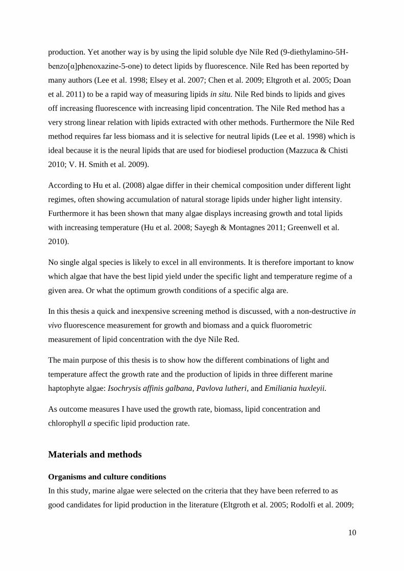
The algae plate is placed on top of the temperature gradient and enclosed by the light gradient

cover. The 96 diode lights are arranged on the cover so that each well receives light from one

diode. This way each row of wells is exposed to the same light and each column of wells the

same temperature.

The algae were grown with 24 hours continuous light for four days except for a 15 min break

each sixth hour, allowing the chip controlling the diode lights to reset. The experiments were

terminated by freezing at -30 C˚. This was done so later measurements could be preformed at

a more convenient time and also to help break open the cells.

An Imaging Pulse Amplitude Modulated Chlorophyll Fluorometer (PAM) (Walz mess- und

Regeltechnik, Effeltrich, Germany) was used to measure in vivo fluorescence from the

growing algae. The advantage of the PAM is that it quickly can do the fluorescence

measurements on all wells of a micro-plate simultaneously, and in a non destructive way so

the algae can quickly be returned to the incubator.

When a chlorophyll a molecule absorbs a photon it is transferred from its low energy ground

state to its high energy excited state. Chlorophyll can only stay in its excited state for a short

time before it has to transfer its energy. If the energy is transmitted to oxygen, damaging

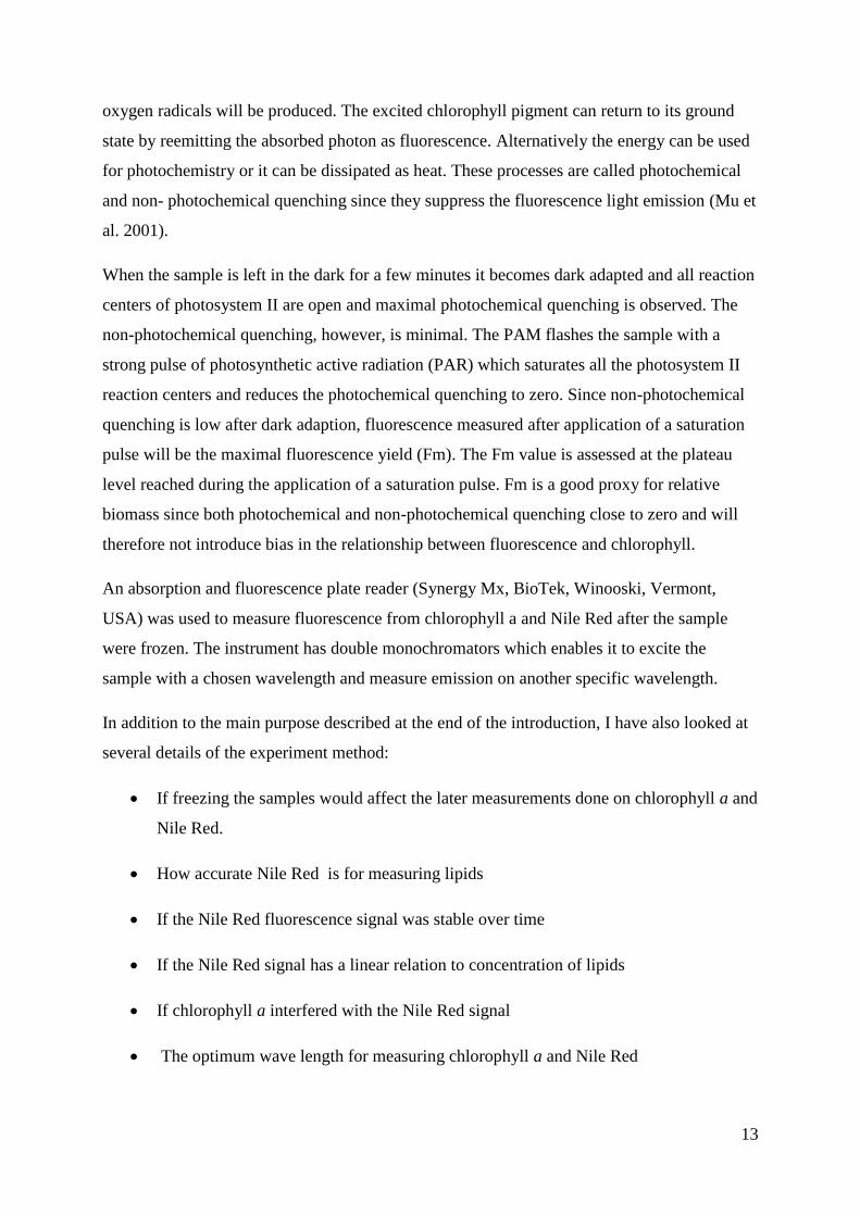
Figure 1 The incubator with a well-plate (left) and the light cover

(right)

13

oxygen radicals will be produced. The excited chlorophyll pigment can return to its ground

state by reemitting the absorbed photon as fluorescence. Alternatively the energy can be used

for photochemistry or it can be dissipated as heat. These processes are called photochemical

and non- photochemical quenching since they suppress the fluorescence light emission (Mu et

al. 2001).

When the sample is left in the dark for a few minutes it becomes dark adapted and all reaction

centers of photosystem II are open and maximal photochemical quenching is observed. The

non-photochemical quenching, however, is minimal. The PAM flashes the sample with a

strong pulse of photosynthetic active radiation (PAR) which saturates all the photosystem II

reaction centers and reduces the photochemical quenching to zero. Since non-photochemical

quenching is low after dark adaption, fluorescence measured after application of a saturation

pulse will be the maximal fluorescence yield (Fm). The Fm value is assessed at the plateau

level reached during the application of a saturation pulse. Fm is a good proxy for relative

biomass since both photochemical and non-photochemical quenching close to zero and will

therefore not introduce bias in the relationship between fluorescence and chlorophyll.

An absorption and fluorescence plate reader (Synergy Mx, BioTek, Winooski, Vermont,

USA) was used to measure fluorescence from chlorophyll a and Nile Red after the sample

were frozen. The instrument has double monochromators which enables it to excite the

sample with a chosen wavelength and measure emission on another specific wavelength.

In addition to the main purpose described at the end of the introduction, I have also looked at

several details of the experiment method:

If freezing the samples would affect the later measurements done on chlorophyll a and

Nile Red.

How accurate Nile Red is for measuring lipids

If the Nile Red fluorescence signal was stable over time

If the Nile Red signal has a linear relation to concentration of lipids

If chlorophyll a interfered with the Nile Red signal

The optimum wave length for measuring chlorophyll a and Nile Red

14

In organizing this thesis, the results from the experiments concerning the methods are

presented consecutively throughout material and method section. The results for the main

experiments are presented in the result section.

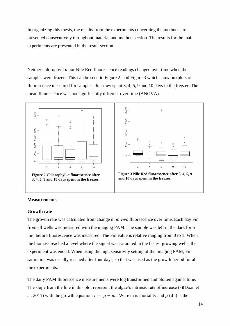
Neither chlorophyll a nor Nile Red fluorescence readings changed over time when the

samples were frozen. This can be seen in Figure 2 and Figure 3 which show boxplots of

fluorescence measured for samples after they spent 3, 4, 5, 9 and 10 days in the freezer. The

mean fluorescence was not significantly different over time (ANOVA).

Measurements

Growth rate

The growth rate was calculated from change in in vivo fluorescence over time. Each day Fm

from all wells was measured with the imaging PAM. The sample was left in the dark for 5

min before fluorescence was measured. The Fm value is relative ranging from 0 to 1. When

the biomass reached a level where the signal was saturated in the fastest growing wells, the

experiment was ended. When using the high sensitivity setting of the imaging PAM, Fm

saturation was usually reached after four days, so that was used as the growth period for all

the experiments.

The daily PAM fluorescence measurements were log transformed and plotted against time.

The slope from the line in this plot represent the algae’s intrinsic rate of increase (r)(Doan et

al. 2011) with the growth equation: . Were m is mortality and (d-1

) is the

Figure 2 Chlorophyll a fluorescence after

3, 4, 5, 9 and 10 days spent in the freezer.

Figure 3 Nile Red fluorescence after 3, 4, 5, 9

and 10 days spent in the freezer.

15

specific growth rate. Assuming mortality is negligible in exponential growth, this plot will

give the specific growth rate of the algae in question. Dividing on the specific growth rate by

the natural log of 2 (0.6931) will give doublings per day.

Biomass

Chlorophyll a fluorescence measured on the plate reader was converted to micrograms

chlorophyll a molecules per liter (µg/L) and used as a proxy for biomass. The assumption is

that the relationship between chlorophyll a and other cell components in the cell is constant.

Therefore a change in chlorophyll a should represent the same change in biomass.

To measure chlorophyll a I used fluorescence. To find the optimum excitation and emission

wave length, I did a small experiment on a standard sample of pure chlorophyll a (Sigma,

lot#BCBF5595V) dissolved in dimethyl sulfoxide (DMSO). The standard sample was excited

with light from 420 to 450 nm and emission from this was measured from 650 to 700 nm,

from this a contour plot was made (Figure 4). The optimum was 430 nm excitation and 675 nm

emission.

Figure 4 Chlorophyll a fluorescence spectrum. Excitation from

420 to 450 nm. Emission measured from 650 to 700 nm.

16

For the real samples the frozen well-plates were thawed and chlorophyll a content was

measured. Each sample was excited with 430 nm light and the fluorescence emission was

measured on 675nm.

Chlorophyll a fluorescence was converted to µg/L via a calibration curve made from the

chlorophyll standard.

Lipid concentration

To measure lipids I used fluorescence from Nile Red (Sigma-Aldrich, N3013). Authors have

used different excitation and emission wavelengths for measuring the Nile Red signal, ranging

from 470 to 549 nm and from 540 to 628 nm, respectively. So finding the right excitation and

emission for a particular medium and

solvent is important.

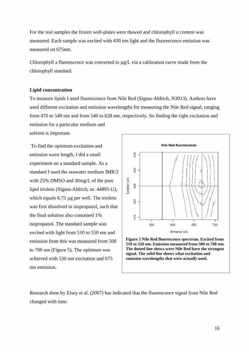
To find the optimum excitation and

emission wave length, I did a small

experiment on a standard sample. As a

standard I used the seawater medium IMR/2

with 25% DMSO and 30mg/L of the pure

lipid triolein (Sigma-Aldrich, nr. 44895-U),

which equals 6.75 µg per well. The triolein

was first dissolved in isopropanol, such that

the final solution also contained 1%

isopropanol. The standard sample was

excited with light from 510 to 550 nm and

emission from this was measured from 500

to 700 nm (Figure 5). The optimum was

achieved with 530 nm excitation and 675

nm emission.

Research done by Elsey et al. (2007) has indicated that the fluorescence signal from Nile Red

changed with time.

Figure 5 Nile Red fluorescence spectrum. Excited from

510 to 550 nm. Emission measured from 500 to 700 nm.

The dotted line shows were Nile Red have the strongest

signal. The solid line shows what excitation and

emission wavelengths that were actually used.

17

To see if Nile Red measurements were stable over time, five concentrations of a standard

(Triolein in IMR/2 with 25% DMSO) were measured every 2 min for 30min in the

spectrophotometer. The same five concentrations were used to make a standard curve as a

check for linearity. I found that the signal did not change within the 30 min timeframe (figure

not shown). The Nile Red standard curve from different triolein concentrations was linear and

the R-squared from a linear model was 0.983.

For the real samples, after chlorophyll a fluorescence was measured; each well was treated

with 25% DMSO (v/v). The DMSO helps break open the cells and homogenize the lipids so

they don’t form droplets. Next the samples were stained with 0.5 µg/mL of Nile Red dye

vortex mixed for 2 min, and then incubated at 37C˚ for 10 min. Figure 5 shows that the

strongest Nile Red signal comes from excitation 530 nm light and measuring emission at 675

nm. However the signal turned out to be unstable when measured on 675 nm and it gave a

poor correlation with the lipid standard. That’s why Nile Red fluorescence was measured with

an excitation wavelength of 530 nm and an emission wavelength of 575 nm as recommended

by Chen et al. (2009).

Lipid calibration

Initial test showed that the more chlorophyll a the sample contained, the less signal was

gained from the Nile Red dye. To explore this, standards with known concentrations of

chlorophyll and triolein were used. Six concentrations of triolein standard in IMR/2 medium

were combined with four concentrations of chlorophyll a standard in DMSO. The triolein

standard was first dissolved in isopropanol and had a final concentration of 1% isopropanol.

The chlorophyll a standard was first dissolved in ethanol and had a final concentration of 2%

ethanol. On 96 well plate 24 different combinations of triolein and chlorophyll was made,

with four replicates of each. First chlorophyll a fluorescence was measured, then Nile Red

dye was added and Nile Red fluorescence was measured.

From this data a linear model was made where Nile Red fluorescence was modeled as a

function of lipid concentration and chlorophyll a fluorescence. From this linear model it was

clear that chlorophyll a interfered with the Nile Red fluorescence.

To adjust for the fact that chlorophyll a lowered the fluorescence emission of Nile Red, a new

linear model was made. Chlorophyll-adjusted lipid content was calculated from the linear

model with lipids as a function of Nile Red (NR) and chlorophyll a (Chl) fluorescence. The

regression gave the formula:

18

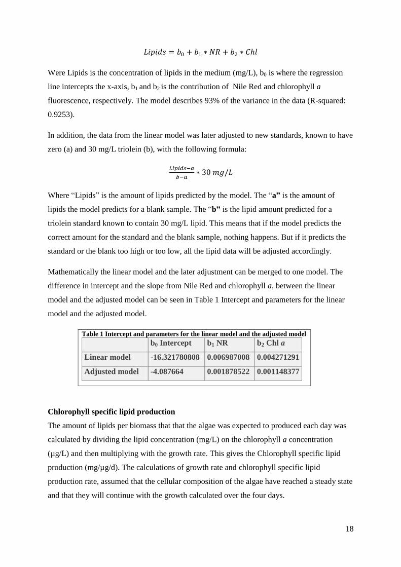
Were Lipids is the concentration of lipids in the medium (mg/L), b0 is where the regression

line intercepts the x-axis, b1 and b2 is the contribution of Nile Red and chlorophyll a

fluorescence, respectively. The model describes 93% of the variance in the data (R-squared:

0.9253).

In addition, the data from the linear model was later adjusted to new standards, known to have

zero (a) and 30 mg/L triolein (b), with the following formula:

Where “Lipids” is the amount of lipids predicted by the model. The “a” is the amount of

lipids the model predicts for a blank sample. The “b” is the lipid amount predicted for a

triolein standard known to contain 30 mg/L lipid. This means that if the model predicts the

correct amount for the standard and the blank sample, nothing happens. But if it predicts the

standard or the blank too high or too low, all the lipid data will be adjusted accordingly.

Mathematically the linear model and the later adjustment can be merged to one model. The

difference in intercept and the slope from Nile Red and chlorophyll a, between the linear

model and the adjusted model can be seen in Table 1 Intercept and parameters for the linear

model and the adjusted model.

Table 1 Intercept and parameters for the linear model and the adjusted model

b0 Intercept b1 NR b2 Chl a

Linear model -16.321780808 0.006987008 0.004271291

Adjusted model -4.087664 0.001878522 0.001148377

Chlorophyll specific lipid production

The amount of lipids per biomass that that the algae was expected to produced each day was

calculated by dividing the lipid concentration (mg/L) on the chlorophyll a concentration

(µg/L) and then multiplying with the growth rate. This gives the Chlorophyll specific lipid

production (mg/µg/d). The calculations of growth rate and chlorophyll specific lipid

production rate, assumed that the cellular composition of the algae have reached a steady state

and that they will continue with the growth calculated over the four days.

19

Statistical methods

Density plots were used to look at the univariate distributions of the response variables. The

plots show the range of values and whether distributions are skewed. Density plots can be

thought of as smoothed histograms using kernel smoothing. The area under the curve always

equals one. One of the advantages of the density plot, is that several distributions can be

compared in one plot.

Scatter plot matrices were used to look at the bivariate relations between light and

temperature, and all the outcome variables. These figures show pair-wise scatter plots with a

loess smoothing line and correlation coefficient for all the variables. Loess (local regression)

is a general method for visualizing nonlinear trends in scatterplots (Cleveland 1979).

To describe the relationship between each outcome variable and light and temperature,

generalized additive models (GAM)(Wood 2006) were used. GAM models are extensions of

generalized linear models, using splines to allow for non-linear effects of the predictors. The

GAM regressions were used to model the response of each outcome variable to the effect of

temperature. Predictions from the GAM models were plotted against temperature in line plots.

The GAM regressions were further used to model the response of each outcome variable to

the combined effect of light and temperature. This way I could account for both possible

confounding and interaction between light and temperature. In the experiment light and

temperature were designed to be independent, but they turned out to be slightly associated.

Predictions from the GAM models were plotted against light and temperature in contour plots.

All data was processed in R programming environment for statistical computing (R

Development Core Team 2010).

20

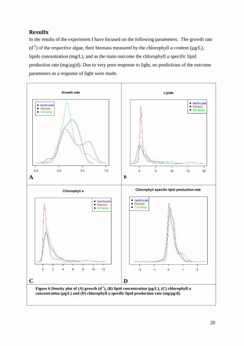
Results In the results of the experiment I have focused on the following parameters: The growth rate

(d-1

) of the respective algae, their biomass measured by the chlorophyll a content (µg/L),

lipids concentration (mg/L), and as the main outcome the chlorophyll a specific lipid

production rate (mg/µg/d). Due to very poor response to light, no predictions of the outcome

parameters as a response of light were made.

A

B

C

D

Figure 6 Density plot of (A) growth (d-1

), (B) lipid concentration (µg/L), (C) chlorophyll a

concentration (µg/L) and (D) chlorophyll a specific lipid production rate (mg/µg/d).

21

Looking at the growth rate distribution for all light and temperature treatments combined, one

can see that distributions for the three alge is between zero and 0.5, although Pavlova also

have a second peek around 0.7. One can also see in the plot that Pavlova reaches the highest

growth rates with Emiliania on a close second (Figure 6 A). For all three species there were

treatments that resulted in negative growth rates. All three distributions are close to

symmetrical.

The lipid concentrations showed a narrow peak from zero to 3mg/L for all three algae. The

long tail shows a few extreme values. Isochrysis achieved the highest lipid concentration of

almost 19 mg/L, Emiliania reached close to 12 mg/L and Pavlova only 7 mg/L. They all also

showed treatments with (meaningless) negative lipid values, Figure 6 B.

The chlorophyll a concentrations were all skewed with tails into high values. Isochrysis

achieved the highest chlorophyll a concentrations Figure 6 C.

The distribution of chlorophyll a specific lipid production rate was remarkably similar for the

three algae. The density curve was centered at 0.5 mg/µg/d, with values reaching out beyond

±2. The negative values are due to the negative growth rates used in the calculation Figure 6

D.

A scatter plot matrix show many parameters plotted pair-wise against each other. The lower

left part of the matrix is the scatter plots with a red loess regression line which describes the

trend in the data. The upper right part is the correlation matrix between the parameters. The

parameter above a scatter plot is the x-axis and the parameter to the right of it is the y-axis.

Light and temperature are not entirely independent in any of the experiments for any of the

species, there is a slight increase in light levels at higher temperatures with a correlation of

0.15 to 0.23 (Figure 7). Also none of the parameters outcomes showed a strong response to

light. The growth response to temperature on the other hand was strong, especially for

Pavlova with a correlation of 0.86. Since chlorophyll a fluorescence was used to calculate

lipids, these two had a strong positive relation.

There was no clear pattern to the relation between chlorophyll a specific lipid production rate

and the other parameters.

22

Figure 7 Scatter plot matrices of light (µE m-2

s-1

),

temperature (C˚), the growth rate mu, chlorophyll

a (µg/L), lipid concentration (mg/L) and lipid per

chlorophyll per day (mg/ µg/d)

23

Due to the weak and erratic response to

light (see discussion) one can use

predictions from the GAM models to plot

the outcome parameters as a function of

temperature and see how they are affected

by temperature (Figure 8).

In all three algae, growth increased with

temperature. Isochrysis reached a plateau

at ca 19 C˚ with a growth rate close to 0.4.

Pavlova reached its plateau at ca 22 C˚

with a growth rate of 0.6. Emiliania did

not reach its plateau in the temperature

range of this experiment. At 24 C˚ it

achieved a growth rate of slightly over 0.3.

The R-squared for this GAM model was

0.51, 0.78 and 0.21 for Isochrysis, Pavlova

and Emiliania respectively.

Lipid normalized to chlorophyll a content

showed a very different response to

temperature for the different algae species.

Emiliania was the species that achieved

the most lipid per chlorophyll. It increased

with temperature to ca 15 C˚ and then

decreased. For Pavlova, the amount of

lipid per chlorophyll decreased with

increasing temperature over the total

range. Isochrysis showed a slow increase

in lipid per chlorophyll with temperature.

(R2

= 0.26, 0.29 and 0.27 for Isochrysis,

Pavlova and Emiliania respectively).

The chlorophyll a specific lipid production

rate increased almost linearly with temperature for Emiliania and Pavlova, and would

Figure 8 Prediction of growth rate, lipids per chlorophyll

and lipids per chlorophyll per day, as a function of

temperature.

24

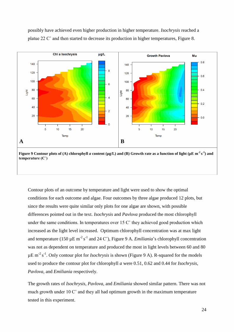
possibly have achieved even higher production in higher temperature. Isochrysis reached a

platue 22 C˚ and then started to decrease its production in higher temperatures, Figure 8.

Contour plots of an outcome by temperature and light were used to show the optimal

conditions for each outcome and algae. Four outcomes by three algae produced 12 plots, but

since the results were quite similar only plots for one algae are shown, with possible

differences pointed out in the text. Isochrysis and Pavlova produced the most chlorophyll

under the same conditions. In temperatures over 15 C˚ they achieved good production which

increased as the light level increased. Optimum chlorophyll concentration was at max light

and temperature (150 µE m-2

s-1

and 24 C˚), Figure 9 A. Emiliania’s chlorophyll concentration

was not as dependent on temperature and produced the most in light levels between 60 and 80

µE m-2

s-1

. Only contour plot for Isochrysis is shown (Figure 9 A). R-squared for the models

used to produce the contour plot for chlorophyll a were 0.51, 0.62 and 0.44 for Isochrysis,

Pavlova, and Emiliania respectively.

The growth rates of Isochrysis, Pavlova, and Emiliania showed similar pattern. There was not

much growth under 10 C˚ and they all had optimum growth in the maximum temperature

tested in this experiment.

A B

Figure 9 Contour plots of (A) chlorophyll a content (µg/L) and (B) Growth rate as a function of light (µE m-2

s-1

) and

temperature (C˚)

25

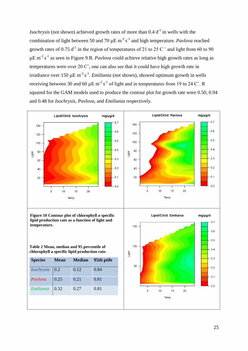
Isochrysis (not shown) achieved growth rates of more than 0.4 d-1

in wells with the

combination of light between 50 and 70 µE m-2

s-1

and high temperature. Pavlova reached

growth rates of 0.75 d-1

in the region of temperatures of 21 to 25 C ˚ and light from 60 to 90

µE m-2

s-1

as seen in Figure 9 B. Pavlova could achieve relative high growth rates as long as

temperatures were over 20 C˚, one can also see that it could have high growth rate in

irradiance over 150 µE m-2

s-1

. Emiliania (not shown), showed optimum growth in wells

receiving between 30 and 60 µE m-2

s-1

of light and in temperatures from 19 to 24 C˚. R

squared for the GAM models used to produce the contour plot for growth rate were 0.50, 0.94

and 0.48 for Isochrysis, Pavlova, and Emiliania respectively.

Table 2 Mean, median and 95 percentile of

chlorophyll a specific lipid production rate.

Species Mean Median 95th ptile

Isochrysis 0.2 0.12 0.84

Pavlova 0.25 0.21 0.81

Emiliania 0.32 0.27 0.81

Figure 10 Contour plot of chlorophyll a specific

lipid production rate as a function of light and

temperature.

26

The chlorophyll a specific lipid production rate for Isochrysis was highest in the highest light

and temperature levels. Pavlova had its highest production in 90 µE m-2

s-1

light and ca 18 C˚

(Figure 10). Emiliania was the one that achieved the highest chlorophyll a specific lipid

production rate, with a mean of 0.32 mg/µg/d .This production occurred above 20 C˚ and with

light from 50 to 70 µE m-2

s-1

Discussion

Summary of the results

For all three algae species light did not give much response, while temperature gave strong a

response. Pavlova was the algae that achieved the highest growth rate, while Isochrysis

produced the most biomass and had the highest lipid concentration. When growth rate,

biomass and lipid concentration was merged to chlorophyll a specific lipid production rate,

Emiliania emerged as the most efficient producer.

The Method and Sources of error

There are several things in this experiment that could lead to uncertainties in the results. Some

are due to methodological weaknesses and some might be mistakes done along the way.

The main uncertainties seemed to be in the lipid predictions. The model I made to predict

lipid concentration from Nile Red fluorescence, predicted a concentration of 30 mg/L from a

fluorescence signal of ca 6600. The standard I later adjusted the model with, of a known

concentration of 30 mg/L lipid gave a fluorescence signal of 18000. It could be that this huge

difference was due to nonlinearities in the signal from very high lipid concentrations. I did

test the linearity of the lipid-Nile Red association, but not that high. Another explanation

could be that by mistake the new standard contained more than the 30 mg/L it was thought to

contain.

27

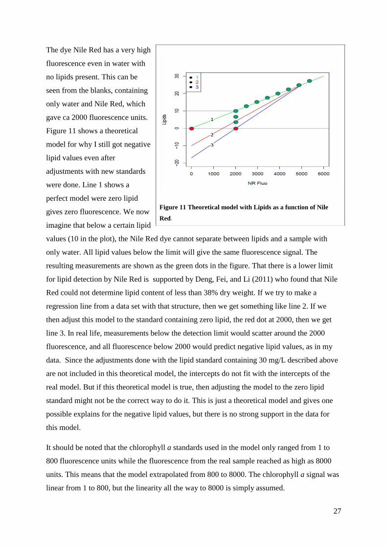
The dye Nile Red has a very high

fluorescence even in water with

no lipids present. This can be

seen from the blanks, containing

only water and Nile Red, which

gave ca 2000 fluorescence units.

Figure 11 shows a theoretical

model for why I still got negative

lipid values even after

adjustments with new standards

were done. Line 1 shows a

perfect model were zero lipid

gives zero fluorescence. We now

imagine that below a certain lipid

values (10 in the plot), the Nile Red dye cannot separate between lipids and a sample with

only water. All lipid values below the limit will give the same fluorescence signal. The

resulting measurements are shown as the green dots in the figure. That there is a lower limit

for lipid detection by Nile Red is supported by Deng, Fei, and Li (2011) who found that Nile

Red could not determine lipid content of less than 38% dry weight. If we try to make a

regression line from a data set with that structure, then we get something like line 2. If we

then adjust this model to the standard containing zero lipid, the red dot at 2000, then we get

line 3. In real life, measurements below the detection limit would scatter around the 2000

fluorescence, and all fluorescence below 2000 would predict negative lipid values, as in my

data. Since the adjustments done with the lipid standard containing 30 mg/L described above

are not included in this theoretical model, the intercepts do not fit with the intercepts of the

real model. But if this theoretical model is true, then adjusting the model to the zero lipid

standard might not be the correct way to do it. This is just a theoretical model and gives one

possible explains for the negative lipid values, but there is no strong support in the data for

this model.

It should be noted that the chlorophyll a standards used in the model only ranged from 1 to

800 fluorescence units while the fluorescence from the real sample reached as high as 8000

units. This means that the model extrapolated from 800 to 8000. The chlorophyll a signal was

linear from 1 to 800, but the linearity all the way to 8000 is simply assumed.

Figure 11 Theoretical model with Lipids as a function of Nile

Red.

28

The chlorophyll a standard was dissolved in ethanol and diluted in DMSO. The real samples

were not exposed to DMSO before after the chlorophyll a was measured on the plate reader.

This means that chlorophyll a molecules were in different mediums in the standard and the

real sample which could lead to different fluorescence emission. It is known that pure

chlorophyll a fluoresce more than chlorophyll a bound to membranes and proteins (Honeywill

& Paterson 2002). Also other pigments that usually transfers their energy to chlorophyll a will

emit fluorescence themselves when not connected in the chloroplast membrane. This means

that compared with the pure chlorophyll standard the chlorophyll a concentration of the real

sample could be underestimated, since the free form of chlorophyll emits more fluorescence.

This again could have lead to an underestimation of the lipids too, since chlorophyll was used

in the model that calculates the lipid concentration. On the other hand when all the accessory

pigments are still bound to the membrane they will transfer their energy to chlorophyll a

which then will emit more fluorescence (Falkowski 1985). The algae samples in my

experiment had been frozen which should lysis the cells, such that the chlorophyll could be

both in free form and bound to membranes. The potential error introduced by the difference

between the standard and the real sample is the same for all the algae species. Hence the

comparison between them should still be valid.

Four of the wells one the 96 well-plate were used for standards. They were there to calculate

the Nile Red fluorescence to lipid concentration, the chlorophyll a fluorescence to µg/L and to

have blanks so the background fluorescence could be removed. They were also meant to

adjust for measuring errors by the plate reader between days. There were several problems

with this. One was that the standards on the plates gave different results on the different

plates, and were therefore not used. The different results is thought to be from human error

were the four standards were not places in the same well number on the different plates.

Therefore new standers were measured and used, which means that the option of mitigating

measuring errors, done by the plate reader, were lost.

The length of the growth period was set to 4 days. This was the time it took for some of the

fastest growing algae to reach a biomass were the signal starts to overflow. Overflow is when

it is too much fluorescence for the PAM to accurately measure. The wells where this happens

will appear to have less fluorescence than what they really have. When then log fluorescence

is plotted as a function of days, the regression line will have a less steep angle when the

fluorescence from the last day is lowered by the overflow. Since the growth rate is calculated

from the angle of the regression line, overflow will lead to underestimation of the growth rate

29

of the algae in wells with the fastest growth. But with a growth period of only four days, this

problem is small.

When the experiment was designed the light was meant to be constant for each row of wells.

Unfortunately the light varied a lot. But, since the light was measured before and after each

experiment and the average values were used, this should not lead to any error.

Although light and temperature were designed independent in the experiment, there were

some correlations between the two. The light levels were higher where the temperature was

high due to a few LEDs in high temperature with very high irradiance. Because the

correlations are so small (0.15, 0.23, and 0.23), light and temperature were treated as

independent parameters in the analysis.

In the experiment, each light and temperature combination was replicated three times. If the

light and temperature had indeed been constant over the three replicates, they would have

been true replicates. Then the mean outcome value over the three replicates could have been

used to reduce measurement error. However, since the light level varied over the replicates,

one could argue that the replicates were in fact independent experiments, with different light

settings. This approach was taken in this thesis, resulting in a three times larger sample size.

The analysis in the thesis (linear models, GAM models) assumed that the units of the sample

(or rather the residuals) were independent. But because of the replicate structure, this was not

entirely true. Mixed effect models would have picked up the correlation structure caused by

the replicates, but the only difference in estimates would have been in the p-values, not in the

model coefficients. Because temperature and light are known to have an effect on biological

systems, p-values are not that important in this thesis. Since ordinary linear models are easier,

they were used to analyze the data. The use of ordinary least squares also made it possible to

use the flexible GAM models.

Chlorophyll a on Nile Red

It is clear from the regression described in the method section, that chlorophyll a interferes

with the Nile Red fluorescence signal. The question is: why is this? And why have so many

authors recommended Nile Red as a strong lipid indicator without correcting for chlorophyll a

interference in their methods?

One explanation for why the Nile red signal is reduced by chlorophyll is that chlorophyll a

maybe do absorb some light in the 530 nm region. According to Taiz & Zeiger (2010)

30

chlorophyll a does not efficiently absorb in the green part of the spectrum, but some is still

absorbed. If that is the case, when a sample is excited with light of 530 nm, both Nile Red and

chlorophyll a will absorb light. When emission is only measured on 570, were chlorophyll has

low emission, only the light absorbed by Nile Red will be reemitted as fluorescence. When

the fluorescence measured from a sample is then compared with the fluorescence from a lipid

standard of a know concentration, the signal from the real sample will be less than that from

the standard even though they have the same lipid concentration. This is because the standard

does not have any other pigments to absorb light, and all the light the standard is exposed to

will be absorbed and reemitted as fluorescence at 570 nm. This phenomenon would only get

stronger if the sample was excited with a wavelength known to be strongly absorbed by

chlorophyll a, like McGinnis & Dempster (1997) who used a excitation of 450 nm and

measured emission on 540 nm. Additional interference could result from chlorophyll a

reabsorbing fluorescence emitted by Nile Red, especially if the emission is measured in a

region were chlorophyll a got strong absorption. I found that Nile Red had its real optimum

fluorescence at 670 nm which probably would have been a poor choice since chlorophyll a

got its second absorption peak on 675. Eltgroth et al. (2005) excited their sample with 492 nm

light and measured emission on 625 nm, were chlorophyll a had pretty high absorption. This

means that both excitation and emission wavelength should be chosen with care.

One could argue that other pigments in the algae were the ones that did the absorbing, but the

regression was done with pure chlorophyll a. Although it could have had a bigger affect in the

real sample where other pigments like β-carotene and chlorophyll b were present too. It

should also be noted that the reduction in Nile Red signal was identified to be due to the

chlorophyll a content in samples with only a maximum chlorophyll a signal of 800

fluorescence units. This shows that chlorophyll a could interfere with Nile Red measurements

in most samples, not only those with extreme chlorophyll a values.

A quick example on how important chlorophyll a was in my model: Using the adjusted

coefficients from the model used to predict lipid concentration, one will get:

Inserting the mean fluorescence signal values of Nile Red (2500) and chlorophyll a (1100)

one will get:

31

Chlorophyll a signal ranged from 0 to ca 8000 fluorescence units in the data, and therefore

had and important effect on the lipid estimates.

Some authors do mention that the chlorophyll a concentration of the sample could be a

problem. Chen et al. (2009) mentions that species with high amount of chlorophyll a it can be

hard to measure lipids with Nile Red using 560/620 nm light because of increased background

fluorescence from chlorophyll. Held & Raymond (2011) argue that using excitation at 530 nm

and emission measured at 570 nm light will minimize background fluorescence from

chlorophyll. Eltgroth et al. (2005) used a Schott glass band-pass output filter to mask

chlorophyll emission. Even though masking the fluorescence from chlorophyll is a good idea

that should be adopted by others, it will not do anything to prevent or take into account the

fact that chlorophyll a will lower the emission from Nile Red. Other authors conclude that

Nile Red can be used accurately to measure lipid concentration, without even discussing the

problem with chlorophyll (Cooksey et al. 1987; Elsey et al. 2007; McGinnis & Dempster

1997; Lee et al. 1998; Deng & Fei 2011). My results suggest that chlorophyll a should be

either be measured and corrected for in Nile Red-based lipid estimates or the chlorophyll

should be bleached before Nile Red is added.

Light response

The algae’s response to light was not as expected. From the scatter plots one can see that the

regression line for growth as a function of light is more or less flat. When growth is plotted as

a function of light one will expect to get a typical light response curve, which has the same

overall structure for all photosynthetic algae (Graham et al. 2009). From the light

compensation point, were the amount of CO2 used in respiration is balanced out by

assimilation, growth should increase close to linearly with increasing light. At a point the

effect of more light on growth will gradually diminish to zero, the algae is said to be light

saturated. The growth is maximal when the algae are light saturated. Further increases in light

after this will have no effect or eventually lead to photo inhibition were growth will be

reduced (Taiz & Zeiger 2010). It is difficult to pinpoint an exact light value for were the

algae’s growth is light saturated because the light response is curved close to maximum

growth. Therefore the term “onset of light saturation” is often used. It is defined as the light

value where the response line intercepts the maximum growth asymptote if the light response

32

was linear all the way. The advantage of onset of light saturation is that it can be compared

between species.

One explanation for why I did not get the expected light response in my experiment, could be

that all the algae were light saturated even in the lowest light levels, without being

photoinhibited in the highest light levels. The amount of light needed to reach light saturation

varies between species, and Talling (1957) propose that it is a result of what depth they

usually grow in. Skjelbred et al. (2012) found onset of light saturation for Pseudochattonella

farcimen with light intensity from 30 to 40 µE m-2

s-1

. Since almost all of my treatments

received light of 30 µE m-2

s-1

or more, they could all be light saturated. Further Ryther (1959)

showed that algae cultivated in flasks at different depths would adapt to the light levels there

and that this could affect the light intensity needed to reach light saturation in later

experiments. Although not measured, the light levels in the culture room were the algae were

stored was low to prevent quick growth and early exhaustion of the growth medium. If that is

the case, the algae could have been adapted to low light levels and therefore reach light

saturation in low light levels.

That the growth was not reduced in the highest irradiance indicates that there were low or no

photoinnhibition. To induce photoinnhibition Leverenz & Falk (1990) exposed their algae

with over 1000 µE m-2

s-1

light, which is substantially more than my highest light level of 150

µE m-2

s-1

. Further is 50% of the photoinnhibition is caused by UV light (Smith & Baker

1980), of which there is none from the LEDs used in the incubator. Marra (1978) reports that

photoinhibition usually only reduce photosynthesis by between 5 and 10%, so if there were

any photoinnhibition in 150 µE m-2

s-1

light, we might not detect it.

Since the in vivo fluorescence was measured every day during the growth period, another

possible explanation for the minimal response to light could be that the well-plate was put

back in the incubator the wrong way. This would lead to a diffuse light response since the

algae would randomly receive high and low irradiance. However, since the light and

temperature gradients in the incubator are at right angles, this type of error should also have

lead to a diffuse temperature response, which was not the case in the experiment. Another

scenario that could lead to no light response would be if the well-plate were sometimes turned

the wrong way when PAM measurements were done. But this would affect the growth rate

calculation. Since the growth rate is calculated by the regression line from log fluorescence as

33

a function of time, the growth rate would be zero if the fluorescence alternated between high

and low.

It should be mentioned that one of the replicates of Emiliania did have closer to expected light

response, but the reasons for this unknown.

Experimental parameters

When selecting an alga for biofuel production, there are many desirable traits. Borowitzka

(1992) states that a key factor for getting production economically viable is screening

microalgae with the right criteria. One problem when looking into the literature on this field,

as Griffiths & Harrison (2009) mentions, is that authors inspect only a few traits and leave out

data that could enable others to compare the traits they are looking for. One example of this is

when only biomass per square meters is reported, without saying how deep the culture vessel

was. This makes it hard to know the biomass per liter. Looking at the main traits for algae,

one can see that they give information on different aspects. Most probably no algae will be

supreme inn all traits, so prioritizing is needed.

Biomass µg/L: Using fluorescence from chlorophyll a as a proxy for biomass has, as

Kruskopf & Flynn (2006) reminds us, some problems. One of them is that shade adapted cells

will have more total chlorophyll a than cells adapted to high irradiance (Taiz & Zeiger 2010).

Further the amount of fluorescence per unit chlorophyll a is known to vary due to sources

such as photoinhibition, photoadaptation, and nutrient limitation (Falkowski 1985). In

addition to this, chlorophyll a fluorescence emission peaks at 675 nm and can be reabsorbed

by other algae. This can lead to less signal per unit chlorophyll a in high concentrations of

algae (Honeywill & Paterson 2002).

Even with its problems, chlorophyll a fluorescence as an approximation of the algae biomass

is considered safe by many (Held 2011). The algae cultures in my study were all grown in the

same light levels before the experiment, and should therefore be adapted to the same light

levels. Some individual adaptation could occur during the four days of growth. In high light

levels algae can also move there chloroplast within the cell to reduce absorption with about

15%, and can therefore adjust to high light levels without reducing their chlorophyll a

concentration (Taiz & Zeiger 2010).

34

Growth rate d-1

: Using in vivo fluorescence to calculate the growth rate should be safe even

with the known variations in chlorophyll a fluorescence. The assumption that the fluorescence

from chlorophyll a linearly correlate with cell number as long as light and temperature are

kept constant and the algae have reached a physiological steady state (Brand et al. 1981; Held

2011). When daily fluorescence is log transformed and plotted as a function of time, the slope

of the last-squares regression line will at least describe the relative increase in chlorophyll a

per day if not the actual increase in biomass.

Lipid concentration mg/L: Assuming the fluorometric estimation of lipid concentration is

correct, it still have some limitations. Lipid concentration tells us about the amount of lipids in

one liter of growth medium. It tells us nothing about how much lipid the algae can be

expected to produce per unit time. Nor does it give information on whether the algae grow

quickly with a low percentage of the weight as lipids or if they grow slowly with high lipid

percentage. Furthermore it does not say if it is high biomass with low lipid content or low

biomass with high lipid content. It is also not possible to compare the lipid concentration

between two experiments since it depends on the start inoculums, which I have not controlled

to be the same.

Lipid per biomass mg/µg: When the lipid concentration is divided on the proxy for biomass,

chlorophyll a, one gets the lipid content which is lipid per biomass. It gives information on

the question if the algae are accumulating lipids in their cells under certain light and

temperature regiments. The ASP program focused their research on algae that could achieve a

dry biomass with a high percentage of lipids. If the growth rate is low in the algae with high

lipid content, the production per day is still low.

Lipid production mg/d: When the lipid concentration is multiplied by the growth rate, the

result is lipid production. It is by many authors considered as the best criteria for choosing

algae (Rodolfi et al. 2009; M. A. Borowitzka 1992). Lipid production is how much lipid the

algae can make per day, which is very important information. However it cannot be compared

between experiments because it is dependent on the biomass it started with. Moreover the

potential lack of information on the amount of biomass that gives this lipid production could

be a problem in downstream processing.

Chlorophyll a specific lipid production rate mg/µg/d: If the lipid content per biomass is

multiplied with the growth rate one will get the chlorophyll a specific lipid production rate,

which is the lipid production per biomass per day. Although the ratio between chlorophyll a

35

and carbon in a algae cell can vary twofold between species (Kruskopf & Flynn 2006), the

chlorophyll a specific lipid production rate can still be compared between species since it can

be thought of as the amount of available photochemical energy that goes through chlorophyll

a that is used to produce lipids, per day.

Depending on what criteria you choose to select for, different algae will come out on top, as

can be seen in the result section. I would argue that chlorophyll a specific lipid production

rate is the best selection criteria. But one also needs information on the growth rate, the

biomass concentration, and the lipid concentration since they all affect the chlorophyll a

specific lipid production rate. Furthermore, if two algae possess the same chlorophyll a

specific lipid production rate, then the other three parameters can be used to select the alga

most suited for your production plant.

In my experiment, selecting for chlorophyll a specific lipid production rate, Emiliania was the

one that preformed the best. Although for future research I would recommend a screening

system optimized for the hybrid system mentioned in the introduction. This could be done by

first screening for algae that have high growth rate and would produce a large biomass in the

photobioreactor. Then screen for algae that accumulates large quantities of lipids under

nutrient deficient conditions in an open raceway pond.

Conclusion

This method is suitable for fast and inexpensive screening of algae for growth rate and

biomass production. The Nile Red dye has potential for lipid detection, but still needs more

research for it to be used with certainty.

36

References

Bligh, E.G. & Dyer, W.J., 1959. A rapid method of total lipid extraction and purification. Canadian

Journal of Biochemistry And Physiology, 37(8), pp.911-917.

Borowitzka, L.J., Borowitzkal, M.A. & Moulton, T.P., 1984. Production and utilization of microalgae

The mass culture of Dunaliella salina for fine chemicals : From laboratory to pilot plant.

Hydrobiologia, 116, pp.115-134.

Borowitzka, M.A., 1992. Algal biotechnology products and processes - matching science and

economics. Journal of Applied Phycology, 4, pp.267-279.

Bozbas, K., 2008. Biodiesel as an alternative motor fuel: Production and policies in the European

Union. Renewable and Sustainable Energy Reviews, 12(2), pp.542-552.

Brand, L.E., Guillard, R.R.L. & Murphy, L.S., 1981. A method for the rapid and precise determination

of acclimated phytoplankton reproduction rates. Journal of Plankton Research, 3(2), pp.193-201.

Charpentier, A.D., Bergerson, J.A. & MacLean, H.L., 2009. Understanding the Canadian oil sands

industry’s greenhouse gas emissions. Environmental Research Letters, 4(1), p.014005.

Chen, W. et al., 2009. A high throughput Nile red method for quantitative measurement of neutral

lipids in microalgae. Journal of Microbiological Methods, 77(1), pp.41-47.

Chisti, Y., 2007. Biodiesel from microalgae. Biotechnology Advances, 25(3), pp.294-306.

Cleveland, W.S., 1979. Robust locally weighted regression and smoothing scatterplots. Journal of the

American Statistical Association, 74(368), pp.829-836.

Cooksey, K.E. et al., 1987. Fluorometric determination of the neutral lipid content of microalgal cells

using Nile Red. Journal of Microbiological Methods, 6(6), pp.333-345.

Deng, X. & Fei, X., 2011. The effects of nutritional restriction on neutral lipid accumulation in

Chlamydomonas and Chlorella. African Journal of Microbiology, 5(3), pp.260-270.

Dismukes, G.C. et al., 2008. Aquatic phototrophs: efficient alternatives to land-based crops for

biofuels. Current Opinion in Biotechnology, 19(3), pp.235-240.

Doan, T.T.Y., Sivaloganathan, B. & Obbard, J.P., 2011. Screening of marine microalgae for biodiesel

feedstock. Biomass and Bioenergy, 35(7), pp.2534-2544.

Doney, S.C. et al., 2009. Ocean Acidification: The Other CO 2 Problem. Annual Review of Marine

Science, 1(1), pp.169-192.

Edvardsen, B., Moy, F. & Paasche, E., 1990. Hemolytic activity in extracts of Chrysochromulina

polylepis grown at different levels of selenite and phosphate. Toxic Marine Phytoplankton,

pp.284-289.

Elsey, D. et al., 2007. Fluorescent measurement of microalgal neutral lipids. Journal of

Microbiological Methods, 68(3), pp.639-642.

37

Eltgroth, M.L., Watwood, R.L. & Wolfe, G.V., 2005. Production and cellular localization of neutral

long-chain lipids in the haptophyte algae Isochrysis galbana and Emiliania huxleyi. Journal of

Phycology, 41(5), pp.1000-1009.

Eppley, R.W., Holmes, W.R. & Strickland, J.D.H., 1967. Sinking rates of marine phytoplankton

measured whit a fluorometer. Journal of Experimental Marine Biology and Ecology, 1, pp.191-

208.

Fairley, P., 2011. Introduction: next generation biofuels. Nature, 474(7352), pp.2-5.

Falkowski, P., 1985. Chlorophyll a fluorescence in phytoplankton: relationship to photosynthesis and

biomass. Journal of Plankton Research, 7(5), pp.715-731.

Graham, L.E., Graham, J.M. & Wilcox, L.W., 2009. Algae Second edi., San Francisco: Pearson

Education.

Graham-Rowe, D., 2011. Agriculture: beyond food versus fuel. Nature, 474(7352), pp.6-8.

Greenwell, H.C. et al., 2010. Placing microalgae on the biofuels priority list: a review of the

technological challenges. Journal of the Royal Society, 7(46), pp.703-726.

Griffiths, M.J. & Harrison, S.T.L., 2009. Lipid productivity as a key characteristic for choosing algal

species for biodiesel production. Journal of Applied Phycology, 21(5), pp.493-507.

Held, P., 2011. Monitoring of algal growth using their intrinsic properties. Biofuel Research.

Held, P. & Raymond, K., 2011. Determination of algal cell lipids using Nile Red using microplates to

monitor neutral lipids in chlorella vulgaris. Biofuel Research.

Honeywill, C. & Paterson, D.M., 2002. Determination of microphytobenthic biomass using pulse-

amplitude modulated minimum fluorescence. European Journal of Phycology, 37(4), pp.485-

492.

Hu, Q. et al., 2008. Microalgal triacylglycerols as feedstocks for biofuel production: perspectives and

advances. The Plant journal : for cell and molecular biology, 54(4), pp.621-39.

Huntley, M.E. & Redalje, D.G., 2007. CO2 Mitigation and renewable oil from photosynthetic

microbes: a new appraisal. Mitigation and Adaptation Strategies for Global Change, 12(4),

pp.573-608.

Imai, I. et al., 1996. Selenium requirement for growth of a novel red tide flagellate Chattonella

verruculosa (Raphidophyceae) in culture. Fisheries Science, 62(5), pp.834–835.

Jimenez, C., 2003. Relationship between physicochemical variables and productivity in open ponds

for the production of Spirulina: a predictive model of algal yield. Aquaculture, 221(1-4), pp.331-

345.

Kirk, J.T.O., 1994. Light and photosynthesis in aquatic ecosystems Second edi., Cambridge university

press.

Knothe, G., 2010. Biodiesel and renewable diesel: a comparison. Progress in Energy and Combustion

Science, 36(3), pp.364-373.

38

Kruskopf, M. & Flynn, K.J., 2006. Chlorophyll content and fluorescence responses cannot be used to

gauge reliably phytoplankton biomass, nutrient status or growth rate. The New Phytologist,

169(3), pp.525-36.

Lee, S.J., Yoon, B.D. & Oh, H.M., 1998. Rapid method for the determination of lipid from the green

alga Botryococcus braunii. Biotechnology Techniques, 12(7), pp.553-556.

Leverenz, J.W. & Falk, S., 1990. The effects of photoinhibition on the photosynthetic light-response

curve of green plant cells (Chlamydomonas reinhardtii). Planta, 182, pp.161-168.

Lewis, T., Nichols, P.D. & McMeekin, T.A., 2000. Evaluation of extraction methods for recovery of

fatty acids from lipid-producing microheterotrophs. Journal of Microbiological Methods, 43(2),

pp.107–116.

Marchetti, J., Miguel, V. & Errazu, A., 2007. Possible methods for biodiesel production. Renewable

and Sustainable Energy Reviews, 11(6), pp.1300-1311.

Marra, J., 1978. Phytoplankton photosynthetic response to vertical movement in a mixed layer. Marine

Biology, 46, pp.203-208.

Martin, J., 2011. Perspective: don’t foul the water. Nature, 474(7352), p.17.

Mazzuca, S.T. & Chisti, Y., 2010. Potential fuel oils from the microalga Choricystis minor. Journal of

Chemical Technology Biotechnology, 85(1), pp.100-108.

McGinnis, K.M. & Dempster, T.A., 1997. Characterization of the growth and lipid content of the

diatom Chaetoceros muelleri. Journal of Applied Phycology, 9, pp.19-24.

Mitchell, D., 2008. A note on rising food prices. World Bank Policy Research.

Mu, P., Li, X.P. & Niyogi, K.K., 2001. Update on photosynthesis non-photochemical quenching . A

response to excess light energy. Plant Physiology, 125, pp.1558-1566.

Pulz, O., 2001. Photobioreactors: production systems for phototrophic microorganisms. Applied

Microbiology Biotechnology, 57(3), pp.287-293.

Rodolfi, L. et al., 2009. Microalgae for oil: strain selection, induction of lipid synthesis and outdoor

mass cultivation in a low-cost photobioreactor. Biotechnology and Bioengineering, 102(1),

pp.100-12.

Ryther, J.H., 1959. Light adaptation by marine phytoplankton. Limnology and Oceanography.

Sanderson, K., 2011. Lignocellulose: a chewy problem. Nature, 474(7352), pp.12-4.

Savage, N., 2011. Fuel options: the ideal biofuel. Nature, 474(7352), pp.9-11.

Sayegh, F.A.Q. & Montagnes, D.J.S., 2011. Temperature shifts induce intraspecific variation in

microalgal production and biochemical composition. Bioresource Technology, 102(3), pp.3007-

3013.

Schnepf, R., 2006. CRS report for congress and agriculture : an overview. Congressional Research

Service.

39

Scott, S.A. et al., 2010. Biodiesel from algae: challenges and prospects. Current Opinion in

Biotechnology, 21(3), pp.1-10.

Searchinger, T. et al., 2008. Use of U.S. croplands for biofuels increases greenhouse gases through

emissions from land-use change. Science, 319(1238), pp.1238-1240.

Sheehan, J., 1998. A look back at the US Department of Energy’s Aquatic Species Program: biodiesel

from algae. National Renewable Energy Laboratory.

Sims, R.E.H. et al., 2010. An overview of second generation biofuel technologies. Bioresource

Technology, 101(6), pp.1570-1580.

Skjelbred, B., Andersen, T. & Edvardsen, B., 2012. A high-throughput method for measuring growth

and respiration in microalgal cultures. Journal of Applied Phycology.

Smith, R.C. & Baker, K.S., 1980. Biologically effective dose transmitted by culture bottles in 14C

productivity experiments. Limnology and Oceanography, 25(2), pp.364-366.

Smith, V.H. et al., 2009. The ecology of algal biodiesel production. Trends in Ecology & Evolution,

25(5), pp.1-9.

Taiz, L. & Zeiger, E., 2010. Plant Physiology Fifth Edit., Sunderland, Massachusetts: Sinauer

Associates.

Talling, J.F., 1957. The phytoplankton population as a compound photosynthetic system. New

Phytologist, 56(2), pp.133-149.

Tilman, D., Hill, J. & Lehman, C., 2006. Carbon-negative biofuels from low-input high-diversity

grassland biomass. Science, 314, pp.1598-1600.

White, S., Anandraj, A. & Bux, F., 2011. PAM fluorometry as a tool to assess microalgal nutrient

stress and monitor cellular neutral lipids. Bioresource Technology, 102(2), pp.1675-1682.

Widdicombe, S. & Spicer, J.I., 2008. Predicting the impact of ocean acidification on benthic

biodiversity: What can animal physiology tell us? Journal of Experimental Marine Biology and

Ecology, 366(2), pp.187-197.

Wood, S.N. 2006. Generalized additive models: an introduction with R. CRC

Yang, J. et al., 2011. Life-cycle analysis on biodiesel production from microalgae: water footprint and

nutrients balance. Bioresource Technology, 102(1), pp.159-165.

Zhu, X.G., Long, S.P. & Ort, D.R., 2008. What is the maximum efficiency with which photosynthesis

can convert solar energy into biomass? Current Opinion in Biotechnology, 19(2), pp.153-159.

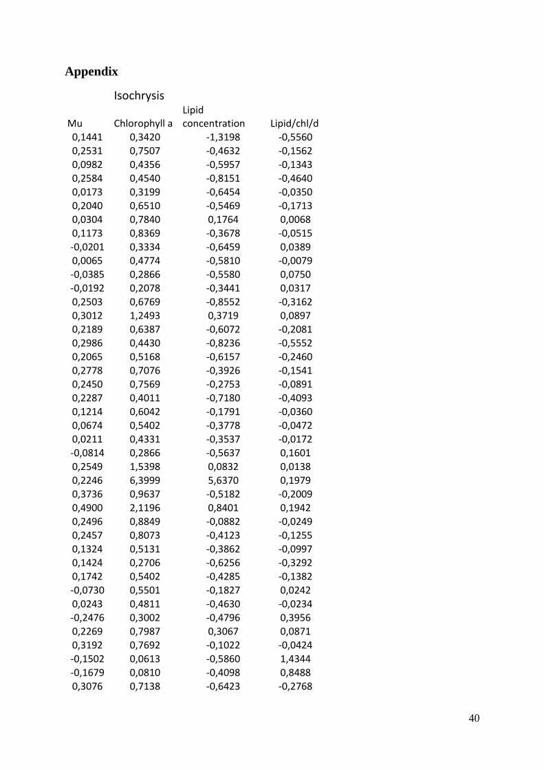
40

Appendix

Isochrysis

Mu Chlorophyll a Lipid concentration Lipid/chl/d

0,1441 0,3420 -1,3198 -0,5560 0,2531 0,7507 -0,4632 -0,1562 0,0982 0,4356 -0,5957 -0,1343 0,2584 0,4540 -0,8151 -0,4640 0,0173 0,3199 -0,6454 -0,0350 0,2040 0,6510 -0,5469 -0,1713 0,0304 0,7840 0,1764 0,0068 0,1173 0,8369 -0,3678 -0,0515

-0,0201 0,3334 -0,6459 0,0389 0,0065 0,4774 -0,5810 -0,0079 -0,0385 0,2866 -0,5580 0,0750 -0,0192 0,2078 -0,3441 0,0317 0,2503 0,6769 -0,8552 -0,3162 0,3012 1,2493 0,3719 0,0897 0,2189 0,6387 -0,6072 -0,2081 0,2986 0,4430 -0,8236 -0,5552 0,2065 0,5168 -0,6157 -0,2460 0,2778 0,7076 -0,3926 -0,1541 0,2450 0,7569 -0,2753 -0,0891 0,2287 0,4011 -0,7180 -0,4093 0,1214 0,6042 -0,1791 -0,0360

0,0674 0,5402 -0,3778 -0,0472 0,0211 0,4331 -0,3537 -0,0172 -0,0814 0,2866 -0,5637 0,1601 0,2549 1,5398 0,0832 0,0138 0,2246 6,3999 5,6370 0,1979 0,3736 0,9637 -0,5182 -0,2009 0,4900 2,1196 0,8401 0,1942 0,2496 0,8849 -0,0882 -0,0249 0,2457 0,8073 -0,4123 -0,1255 0,1324 0,5131 -0,3862 -0,0997 0,1424 0,2706 -0,6256 -0,3292 0,1742 0,5402 -0,4285 -0,1382

-0,0730 0,5501 -0,1827 0,0242 0,0243 0,4811 -0,4630 -0,0234 -0,2476 0,3002 -0,4796 0,3956 0,2269 0,7987 0,3067 0,0871 0,3192 0,7692 -0,1022 -0,0424 -0,1502 0,0613 -0,5860 1,4344 -0,1679 0,0810 -0,4098 0,8488 0,3076 0,7138 -0,6423 -0,2768

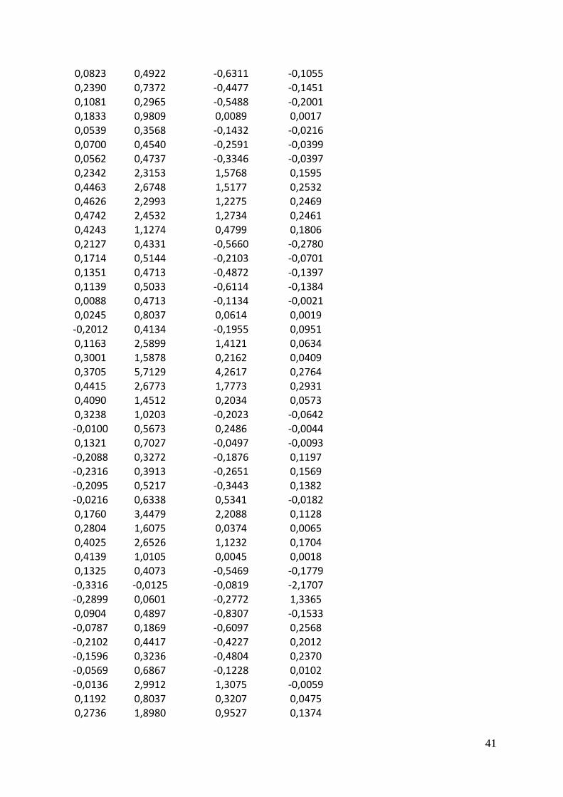
41

0,0823 0,4922 -0,6311 -0,1055

0,2390 0,7372 -0,4477 -0,1451 0,1081 0,2965 -0,5488 -0,2001 0,1833 0,9809 0,0089 0,0017 0,0539 0,3568 -0,1432 -0,0216 0,0700 0,4540 -0,2591 -0,0399 0,0562 0,4737 -0,3346 -0,0397 0,2342 2,3153 1,5768 0,1595 0,4463 2,6748 1,5177 0,2532 0,4626 2,2993 1,2275 0,2469 0,4742 2,4532 1,2734 0,2461 0,4243 1,1274 0,4799 0,1806 0,2127 0,4331 -0,5660 -0,2780

0,1714 0,5144 -0,2103 -0,0701 0,1351 0,4713 -0,4872 -0,1397 0,1139 0,5033 -0,6114 -0,1384 0,0088 0,4713 -0,1134 -0,0021 0,0245 0,8037 0,0614 0,0019 -0,2012 0,4134 -0,1955 0,0951 0,1163 2,5899 1,4121 0,0634 0,3001 1,5878 0,2162 0,0409 0,3705 5,7129 4,2617 0,2764 0,4415 2,6773 1,7773 0,2931 0,4090 1,4512 0,2034 0,0573 0,3238 1,0203 -0,2023 -0,0642

-0,0100 0,5673 0,2486 -0,0044 0,1321 0,7027 -0,0497 -0,0093 -0,2088 0,3272 -0,1876 0,1197 -0,2316 0,3913 -0,2651 0,1569

-0,2095 0,5217 -0,3443 0,1382 -0,0216 0,6338 0,5341 -0,0182 0,1760 3,4479 2,2088 0,1128 0,2804 1,6075 0,0374 0,0065 0,4025 2,6526 1,1232 0,1704 0,4139 1,0105 0,0045 0,0018 0,1325 0,4073 -0,5469 -0,1779 -0,3316 -0,0125 -0,0819 -2,1707 -0,2899 0,0601 -0,2772 1,3365

0,0904 0,4897 -0,8307 -0,1533 -0,0787 0,1869 -0,6097 0,2568 -0,2102 0,4417 -0,4227 0,2012 -0,1596 0,3236 -0,4804 0,2370 -0,0569 0,6867 -0,1228 0,0102 -0,0136 2,9912 1,3075 -0,0059 0,1192 0,8037 0,3207 0,0475 0,2736 1,8980 0,9527 0,1374

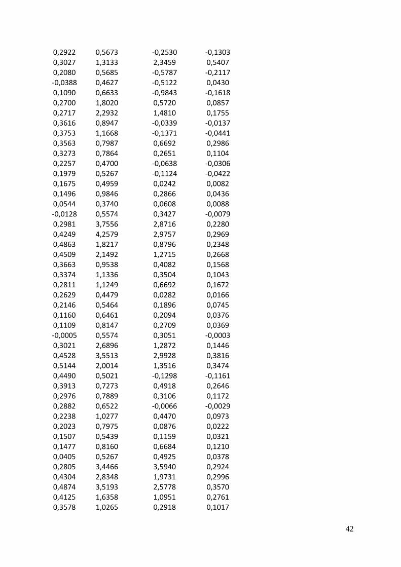
42

0,2922 0,5673 -0,2530 -0,1303

0,3027 1,3133 2,3459 0,5407 0,2080 0,5685 -0,5787 -0,2117 -0,0388 0,4627 -0,5122 0,0430 0,1090 0,6633 -0,9843 -0,1618 0,2700 1,8020 0,5720 0,0857 0,2717 2,2932 1,4810 0,1755 0,3616 0,8947 -0,0339 -0,0137 0,3753 1,1668 -0,1371 -0,0441 0,3563 0,7987 0,6692 0,2986 0,3273 0,7864 0,2651 0,1104 0,2257 0,4700 -0,0638 -0,0306 0,1979 0,5267 -0,1124 -0,0422

0,1675 0,4959 0,0242 0,0082 0,1496 0,9846 0,2866 0,0436 0,0544 0,3740 0,0608 0,0088 -0,0128 0,5574 0,3427 -0,0079 0,2981 3,7556 2,8716 0,2280 0,4249 4,2579 2,9757 0,2969 0,4863 1,8217 0,8796 0,2348 0,4509 2,1492 1,2715 0,2668 0,3663 0,9538 0,4082 0,1568 0,3374 1,1336 0,3504 0,1043 0,2811 1,1249 0,6692 0,1672 0,2629 0,4479 0,0282 0,0166

0,2146 0,5464 0,1896 0,0745 0,1160 0,6461 0,2094 0,0376 0,1109 0,8147 0,2709 0,0369 -0,0005 0,5574 0,3051 -0,0003

0,3021 2,6896 1,2872 0,1446 0,4528 3,5513 2,9928 0,3816 0,5144 2,0014 1,3516 0,3474 0,4490 0,5021 -0,1298 -0,1161 0,3913 0,7273 0,4918 0,2646 0,2976 0,7889 0,3106 0,1172 0,2882 0,6522 -0,0066 -0,0029 0,2238 1,0277 0,4470 0,0973 0,2023 0,7975 0,0876 0,0222

0,1507 0,5439 0,1159 0,0321 0,1477 0,8160 0,6684 0,1210 0,0405 0,5267 0,4925 0,0378 0,2805 3,4466 3,5940 0,2924 0,4304 2,8348 1,9731 0,2996 0,4874 3,5193 2,5778 0,3570 0,4125 1,6358 1,0951 0,2761 0,3578 1,0265 0,2918 0,1017

43

0,3245 0,6412 0,0733 0,0371

0,2931 0,5390 0,0118 0,0064 0,2165 0,8295 0,1344 0,0351 0,2095 1,0548 0,2882 0,0572 0,1218 0,5070 0,4741 0,1139 0,1331 1,1336 0,7449 0,0875 0,0322 0,5513 0,4779 0,0279 0,3896 6,0466 5,6155 0,3618 0,5214 7,0461 7,2017 0,5329 0,5255 3,6510 4,3050 0,6196 0,4708 2,1270 1,9346 0,4282 0,3497 1,3379 1,0914 0,2853 0,3278 0,6091 0,4022 0,2165

0,2448 1,1225 0,0395 0,0086 0,1658 0,9932 0,1406 0,0235 0,2015 0,9058 0,0497 0,0110 0,1600 0,6670 0,1162 0,0279 0,1811 0,6596 0,3835 0,1053 0,0641 0,3346 0,2513 0,0481 0,2905 6,2928 5,5840 0,2578 0,3071 4,7294 4,5069 0,2927 0,5010 3,5180 4,5829 0,6526 0,4178 2,3769 2,4871 0,4372 0,4013 1,1225 0,3194 0,1142 0,3404 2,7917 3,0244 0,3687

0,2431 0,6461 -0,0198 -0,0075 0,2201 0,7803 -0,0825 -0,0233 0,1777 0,5230 0,0400 0,0136 0,1922 0,9563 0,3673 0,0738

0,1446 0,9945 1,0453 0,1520 0,0590 0,4023 0,4028 0,0591 0,3861 4,7626 7,0007 0,5676 0,4051 8,6169 9,4860 0,4460 0,4810 4,4315 5,5778 0,6054 0,4464 2,0704 2,0753 0,4474 0,4411 1,9817 1,0571 0,2353 0,2476 1,7983 2,2085 0,3041 0,2104 0,6966 0,2151 0,0650

0,1401 0,6338 0,2279 0,0504 0,0884 0,5205 0,3439 0,0584 0,1336 0,6916 0,1974 0,0381 0,1048 0,7704 0,4794 0,0652 0,0400 0,6079 0,2696 0,0177 0,2921 8,6280 9,3311 0,3159 0,3017 4,2197 4,5481 0,3252 0,4228 3,2349 3,6595 0,4783

44

0,3836 0,7483 0,1243 0,0637

0,2688 1,1065 1,7660 0,4289 0,1096 0,4971 0,3822 0,0843 0,0944 0,6325 0,4917 0,0734 0,0853 0,7384 0,3725 0,0430 0,3143 1,5287 4,0703 0,8370 0,3501 2,7893 4,7353 0,5944 0,2713 1,3441 1,7396 0,3512 0,4065 2,5615 2,9505 0,4682 0,1984 0,9317 1,0713 0,2281 0,2806 1,1040 0,9897 0,2515 0,1723 0,8947 1,0800 0,2080 0,2263 0,9403 0,8877 0,2136

0,1137 0,8837 0,6282 0,0808 0,1074 1,1040 0,7681 0,0747 0,0364 0,9723 0,4254 0,0159 0,0440 1,2370 0,9747 0,0346 0,4170 2,1898 5,2768 1,0049 0,3604 1,5792 3,6290 0,8282 0,3698 1,7023 2,2072 0,4795 0,3988 2,1344 1,9547 0,3652 0,3486 1,6580 1,3468 0,2832 0,3898 2,5098 2,2392 0,3478 0,3268 1,9756 1,7389 0,2876 0,3120 1,0055 0,8659 0,2687

0,2562 1,1397 1,1470 0,2578 0,1249 1,1520 0,8297 0,0900 0,1635 2,3215 2,1029 0,1481 0,0866 1,2013 0,8926 0,0643

0,3948 3,9243 8,6325 0,8684 0,4617 8,7585 15,2180 0,8023 0,4660 3,2103 3,9108 0,5677 0,5642 5,1935 5,6856 0,6177 0,3910 2,1996 1,8540 0,3296 0,3763 2,2969 2,6886 0,4404 0,3171 1,9694 2,0788 0,3347 0,2441 1,4278 1,5848 0,2709 0,2437 1,1373 1,3401 0,2871

0,1000 1,5164 1,8290 0,1207 0,1391 2,7720 2,7468 0,1378 0,0914 2,3880 2,5444 0,0974 0,4074 3,4479 7,5720 0,8947 0,4598 8,4532 13,4980 0,7343 0,5297 3,8356 5,6043 0,7740 0,2479 1,1471 1,2910 0,2790 0,3797 2,1258 1,9842 0,3544

45

0,2445 1,0511 1,3686 0,3184

0,3480 1,7368 1,1536 0,2312 0,3287 1,7269 1,6816 0,3201 0,2697 1,6075 1,7806 0,2988 0,0754 1,4364 2,3762 0,1248 0,1500 3,2681 3,0536 0,1402 0,0956 1,3859 2,2258 0,1535 0,3385 5,3584 11,1464 0,7042 0,5365 10,1569 16,6578 0,8799 0,5746 5,9505 9,8427 0,9505 0,5739 5,0026 7,2509 0,8318 0,4493 2,1528 4,5079 0,9409 0,3709 2,0162 3,3773 0,6213

0,3209 1,7811 2,9814 0,5372 0,2038 1,4192 2,6362 0,3785 0,2774 1,6531 2,2740 0,3816 0,1387 1,6888 1,3793 0,1133 0,1314 3,1426 3,5564 0,1487 0,0475 1,6407 2,1347 0,0618 0,2468 7,8685 15,4810 0,4855 0,4012 11,0272 18,4616 0,6716 0,5247 7,2665 12,5901 0,9090 0,4820 4,5275 8,0606 0,8581 0,4583 3,0441 5,3900 0,8115 0,3683 1,9645 2,7129 0,5087

0,3437 1,8439 2,7431 0,5113 0,3527 1,8993 2,3778 0,4416 0,2172 2,0827 2,1563 0,2249 0,2597 2,3584 2,1599 0,2379

0,0445 2,8755 2,7343 0,0423 -0,0270 1,5472 2,0550 -0,0358 0,3688 11,2722 17,7978 0,5822 0,4102 9,3444 14,5248 0,6376 0,4114 8,8496 16,3606 0,7605 0,5051 6,2017 12,9399 1,0539 0,5077 3,0773 5,2877 0,8724 0,3508 2,3646 4,0648 0,6031 0,3812 2,2255 3,8299 0,6560

0,3422 2,0100 2,9226 0,4976 0,1940 1,4438 3,0650 0,4118 0,2363 1,5558 1,6216 0,2463 0,0319 1,4930 1,8842 0,0403 -0,1018 1,9522 2,6319 -0,1373 0,2661 9,8676 16,3034 0,4397 0,3836 9,5746 15,3275 0,6141 0,4819 8,2144 16,9721 0,9956

46

0,3300 1,4216 1,9980 0,4637

0,3997 2,9789 5,3367 0,7161 0,2754 2,5185 3,7406 0,4090 0,1738 1,4450 2,2452 0,2700 0,1227 1,2653 2,3462 0,2275

Pavlova

Mu Chlorophyll a

Lipid concentration Lipid/chl/d

0,3176 0,2669 0,7555 0,8990 0,6627 1,1594 -0,0575 -0,0329 0,3084 0,1894 0,6080 0,9900

0,6334 0,3753 -0,5599 -0,9450 0,2616 0,2780 0,4465 0,4202 0,4008 0,4048 -0,1134 -0,1123 0,2753 0,1241 -0,0014 -0,0031 0,3263 0,3703 0,4725 0,4163 0,2054 0,2460 0,1442 0,1204 0,1518 0,3531 0,8622 0,3706 0,1806 0,1783 1,1424 1,1569 0,1103 0,3950 0,7528 0,2103 0,4600 0,4294 1,1043 1,1830 0,3744 0,2719 0,4745 0,6535 0,4409 0,3482 0,1043 0,1320

0,5527 0,5833 -0,0878 -0,0832 0,4253 0,3999 0,5470 0,5818 0,4922 0,7741 0,3927 0,2497 0,4179 0,4848 1,0076 0,8685 0,3030 0,2620 0,0972 0,1123 0,2269 0,2312 0,5043 0,4948 0,1932 0,2731 0,4062 0,2874 0,1683 0,2915 0,6751 0,3897 0,1609 0,7692 1,2259 0,2564 0,6431 1,2702 0,9945 0,5035 0,7135 1,7725 1,5757 0,6343 0,6028 1,0154 0,7323 0,4348 0,6718 1,0646 0,5829 0,3678

0,4907 0,4430 0,1401 0,1552 0,2452 0,5747 0,7439 0,3174 0,3707 0,5464 0,6423 0,4358 0,1290 0,7643 1,0748 0,1814 0,2189 0,5365 0,2912 0,1188 0,0326 0,4873 0,7581 0,0507 0,1413 0,5648 0,8718 0,2181 0,1074 0,2472 0,3501 0,1521

47

0,6538 0,9255 0,0436 0,0308

0,6939 1,6506 1,4038 0,5901 0,6798 0,4737 -0,1092 -0,1567 0,2541 0,3826 -0,0608 -0,0404 0,4950 0,6904 0,4254 0,3050 0,2440 0,2411 1,8754 1,8984 0,3876 0,5735 0,7108 0,4804 0,2914 0,3531 0,5165 0,4262 0,1750 0,3986 0,4688 0,2058 0,0083 0,5870 1,0597 0,0149 0,1265 0,4799 1,0650 0,2807 0,0919 1,2197 1,6650 0,1255 0,5786 2,1381 1,6162 0,4374

0,7356 3,5882 3,2827 0,6730 0,7507 1,2739 0,2766 0,1630 0,6955 0,5796 0,3784 0,4541 0,4938 1,4019 1,9965 0,7033 0,2528 1,0277 3,2798 0,8068 0,2259 0,8307 1,9314 0,5252 0,0608 0,7470 1,1846 0,0964 0,1450 0,3223 0,5705 0,2567 0,0262 0,2645 0,5540 0,0550 0,1305 0,9452 1,4089 0,1945 0,0557 0,3026 0,6422 0,1182 0,4246 3,6584 2,8842 0,3348

0,6105 3,4491 3,1548 0,5584 0,7000 2,3523 1,0853 0,3230 0,5681 1,1865 2,1562 1,0324 0,4530 1,2296 1,6047 0,5912

0,2143 0,9526 1,9812 0,4458 0,2057 0,9501 1,8343 0,3971 0,3092 0,5390 0,7049 0,4043 0,0466 0,4220 0,8269 0,0914 0,1399 0,5365 0,7083 0,1847 0,0148 0,1832 0,8709 0,0704

-0,0089 0,1389 0,8295 -0,0534 0,6633 3,5784 3,8296 0,7098

0,6494 4,5386 4,2895 0,6138 0,6563 3,4590 3,2035 0,6078 0,5629 2,0974 2,7392 0,7352 0,5384 1,3318 1,8784 0,7594 0,1603 1,4229 2,4030 0,2707 0,2429 0,8086 1,1574 0,3477 0,2436 0,8726 0,7682 0,2144 0,0835 0,4553 0,6625 0,1215

48

0,1733 0,4220 0,8908 0,3658

0,0137 0,3556 0,5094 0,0197 -

0,0872 0,6362 0,8314 -0,1140 0,5863 6,9181 6,9958 0,5929 0,6148 3,1389 3,4102 0,6679 0,6424 2,8607 2,3467 0,5270 0,3708 0,3937 0,9733 0,9166 0,4352 1,0572 3,5929 1,4788 0,1226 0,8123 3,9599 0,5978 0,0935 0,5045 1,1762 0,2179 0,0316 0,4590 0,9121 0,0628 0,1527 0,0958 0,4042 0,6442

0,5647 0,5193 0,2395 0,2604 0,2019 0,0860 -0,0032 -0,0075 0,5095 0,5390 0,2954 0,2793 0,1465 0,0466 0,2061 0,6485

0,2783 0,0860 0,1584 0,5127 0,1856 0,0872 0,3981 0,8471 0,2005 0,0934 0,1371 0,2943 0,1491 0,1918 0,2984 0,2320 0,0765 0,2177 0,5236 0,1839 0,0601 0,0626 0,3112 0,2990 0,0251 0,2398 0,4353 0,0456 0,3066 0,1992 0,6416 0,9873

0,2364 0,1451 0,5948 0,9695 0,3313 0,4048 -0,0308 -0,0252 0,4324 0,4233 0,2814 0,2875 0,3183 0,1623 -0,2326 -0,4561 0,3571 0,4085 0,2038 0,1781 0,2762 0,1020 0,0211 0,0572 0,1714 0,1574 0,3339 0,3636 0,1316 0,1980 -0,2669 -0,1774 0,0899 0,0663 -0,0704 -0,0955 0,0812 0,2792 0,3293 0,0958 0,0308 0,2238 0,3358 0,0463 0,6275 0,4565 0,2448 0,3365 0,7836 1,1237 0,8108 0,5654

0,5106 0,4577 0,4695 0,5237 0,5823 0,5008 -0,0032 -0,0037 0,3901 0,1943 -0,1294 -0,2599 0,2788 0,6202 0,5591 0,2513 0,2834 0,2768 0,3288 0,3367 0,0716 0,2152 0,6640 0,2210 0,1368 0,3457 0,3143 0,1243 0,0020 0,5131 0,6019 0,0023

49

0,1019 0,2078 0,3190 0,1564

0,0304 0,1204 -0,0668 -0,0168 0,5770 0,1783 0,0322 0,1042 0,7674 0,7581 0,4942 0,5003 0,5731 0,3753 0,2084 0,3183 0,1720 0,1192 -0,0755 -0,1090 0,3787 0,3740 0,0213 0,0216 0,1894 0,2435 0,1363 0,1060 0,2578 0,3568 0,3114 0,2250 0,1761 0,2829 0,2031 0,1264 0,0806 0,3703 0,1531 0,0333

-0,0201 0,6239 0,7203 -0,0232

0,0721 0,2091 0,3371 0,1162 0,0328 0,1291 0,4465 0,1134 0,7305 0,8184 0,1034 0,0923 0,7759 1,2173 0,9319 0,5940

0,6796 0,9698 0,4456 0,3123 0,5864 0,9821 0,9793 0,5847 0,4514 0,5353 0,3558 0,3001 0,2573 0,3900 0,4984 0,3287 0,1445 0,2669 0,5488 0,2971 0,0292 0,3125 0,5913 0,0553 0,0558 0,3236 0,1865 0,0322

-0,0106 0,1254 0,0448 -0,0038 0,0511 0,2620 0,4973 0,0970 0,0016 0,1660 0,4340 0,0041 0,6371 1,2961 0,2691 0,1323 0,7539 1,4376 0,5289 0,2773 0,7240 1,2985 0,3352 0,1869 0,4855 1,0659 0,7719 0,3516 0,4381 0,4257 0,2743 0,2823 0,2441 0,6153 0,9715 0,3854 0,1540 0,5107 0,7781 0,2347 0,1878 0,2608 -0,1181 -0,0851 0,0122 0,2238 0,2100 0,0114 0,0523 0,2719 0,3355 0,0645

-0,0489 0,0823 0,2902 -0,1725

-0,0783 0,0823 0,7222 -0,6876 0,7288 2,5492 0,5327 0,1523 0,7002 0,9292 0,0884 0,0666 0,6190 1,4278 0,3900 0,1691 0,4602 1,2961 1,2853 0,4564

50

0,4597 0,4725 0,2823 0,2746

0,1478 0,4750 -0,1607 -0,0500 0,1704 0,1758 0,0525 0,0508 0,1144 0,3716 0,6145 0,1892 0,0056 0,1131 0,4184 0,0207 0,0478 0,2165 0,4999 0,1105

-0,0561 0,0970 0,7604 -0,4399

-0,1007 0,0577 0,4269 -0,7458 0,6192 1,2320 0,4085 0,2053 0,6559 1,1102 1,2152 0,7180 0,5927 0,5993 0,4851 0,4797

0,2238 0,1808 0,5567 0,6894 0,3080 0,2731 2,1231 2,3946 0,1360 0,4134 0,1069 0,0352 0,0303 0,1315 0,6216 0,1435

-0,0391 0,1106 0,3936 -0,1391 0,4048 0,3556 0,7160 0,8153 0,6368 1,7146 0,8474 0,3147 0,3852 0,4590 0,4105 0,3445 0,6274 1,4425 0,3362 0,1462 0,3193 0,4380 0,5920 0,4315 0,4287 0,6769 0,4222 0,2674

0,2800 0,4479 -0,6649 -0,4157 0,2733 0,5698 0,2227 0,1068 0,1902 0,3703 0,4687 0,2407 0,1106 0,3359 0,1567 0,0516 0,1523 0,2066 0,5095 0,3757 0,1334 0,1549 0,4425 0,3811 0,5206 0,6338 0,5867 0,4820 0,4540 0,5131 0,3201 0,2833 0,4931 0,7778 0,3529 0,2237 0,5601 1,4955 -0,2306 -0,0864 0,4490 0,9846 0,5120 0,2335 0,4641 1,1397 0,9610 0,3914 0,3441 0,8763 0,2663 0,1046

0,2462 0,7150 0,3432 0,1182 0,2014 0,6695 0,8849 0,2662 0,1606 0,3753 0,7288 0,3119 0,1519 0,2792 0,2335 0,1270 0,0932 0,1684 0,4307 0,2383 0,7244 1,9411 0,4012 0,1497 0,6707 4,1963 2,8657 0,4580 0,6295 1,6395 0,6308 0,2422

51

0,6754 2,7277 1,3566 0,3359

0,4761 1,1619 0,2885 0,1182 0,2900 1,1496 1,5488 0,3907 0,3055 0,8849 0,4472 0,1544 0,0689 0,6695 0,3739 0,0385 0,1618 0,6387 0,4692 0,1189 0,0092 0,4577 0,5596 0,0112 0,1214 0,4245 0,1229 0,0351 0,0801 0,3408 0,6065 0,1425 0,6598 1,5989 0,4820 0,1989 0,6492 4,5792 2,7476 0,3895 0,6901 2,2673 0,9948 0,3028 0,2862 0,3962 -0,0707 -0,0511

0,4827 1,3650 -0,0762 -0,0269 0,2655 0,7667 0,4365 0,1511 0,3066 0,9428 0,4335 0,1410 0,2138 0,8381 -0,0135 -0,0034 0,1114 0,7753 0,5610 0,0806

-0,0403 0,4614 0,5875 -0,0513 0,1317 0,3125 0,4072 0,1716 0,0824 0,3445 0,7433 0,1777 0,6352 6,1143 3,9936 0,4149 0,7904 4,1114 2,2774 0,4378 0,7567 2,9025 1,2173 0,3174

0,6552 2,4741 0,9341 0,2474 0,5010 2,0654 0,3800 0,0922 0,2856 1,2702 0,6037 0,1358 0,1630 0,9600 0,3237 0,0550 0,0204 0,7803 0,4360 0,0114 0,0854 0,7569 0,5381 0,0607

-0,0178 0,7224 0,3820 -0,0094 0,0494 0,6732 0,5991 0,0440 0,0284 0,2435 0,6510 0,0758 0,5608 4,5607 2,4974 0,3071 0,5551 4,2062 1,7891 0,2361 0,7597 3,7101 1,5179 0,3108

0,5202 2,8804 1,2323 0,2226 0,4735 1,9596 0,7434 0,1796 0,2519 1,2530 1,4461 0,2907 0,1597 0,9366 0,6701 0,1143 0,2200 0,8320 0,2776 0,0734 0,0313 0,7483 0,2803 0,0117 0,0706 0,5279 -0,1038 -0,0139

- 0,4233 0,0785 -0,0134

52

0,0721

-0,0711 0,1684 -0,3114 0,1315 0,6676 3,4873 2,4090 0,4612 0,6814 3,8873 2,3821 0,4175 0,6654 3,8209 1,8654 0,3249 0,5066 3,0035 1,7811 0,3004 0,5028 2,0716 1,8059 0,4383 0,1507 1,1323 0,8903 0,1185 0,1750 1,3071 0,8505 0,1139 0,0972 0,8874 0,9811 0,1074

-0,0250 0,4208 0,9422 -0,0560

0,0301 0,4836 1,1680 0,0728 -

0,1137 0,3974 0,8997 -0,2574 -

0,1580 0,2128 0,3931 -0,2919 0,6097 3,4466 1,4468 0,2560 0,6226 3,4639 1,0910 0,1961 0,6136 3,8615 1,8395 0,2923 0,3748 0,6990 -1,0356 -0,5552 0,3276 1,6961 0,5728 0,1106 0,1112 0,9440 -0,1740 -0,0205

-0,0057 0,9058 0,6978 -0,0044

-0,0761 0,7150 0,2849 -0,0303

Emiliania

Mu Chlorophyll a Lipid concentration Lipid/chl/d

0,0070 0,4122 1,6198 0,0275 0,4152 1,1299 1,0458 0,3843 0,1127 0,7926 1,1594 0,1648 0,3997 1,4032 0,5794 0,1650 0,0607 0,4380 0,7874 0,1090

0,1729 0,5341 0,9840 0,3186 0,0448 0,4159 0,8869 0,0956 0,2035 0,5501 1,9495 0,7211 0,0655 0,3531 1,2754 0,2367 0,1712 0,2546 0,6162 0,4143 0,0229 0,3334 0,3535 0,0243 0,1379 0,3765 0,1645 0,0602 0,2100 0,7889 1,1334 0,3018 0,1322 1,6284 2,3994 0,1948

53

0,2441 0,8997 1,6350 0,4436

0,3703 1,5115 1,5746 0,3858 0,2420 1,3958 1,5305 0,2654 0,2961 1,1976 0,5585 0,1381 0,1938 0,6645 0,3656 0,1066 0,2209 0,7680 0,6574 0,1891 0,1689 0,6756 0,4623 0,1156 0,0586 0,4836 0,7829 0,0948 0,2114 1,1520 1,2111 0,2222 0,0920 0,5316 0,1026 0,0178 0,4158 1,3896 1,7483 0,5232 0,4334 3,3506 4,3704 0,5653 0,4091 1,6186 1,6576 0,4190

0,5632 2,5702 1,3073 0,2865 0,2730 1,5706 1,9115 0,3323 0,2957 0,7519 1,3620 0,5356 0,1868 0,7753 0,7451 0,1795 0,2655 0,8541 0,7359 0,2287 0,2296 0,6769 1,4009 0,4752 0,1067 1,1299 1,3012 0,1228 0,2940 1,1360 0,9707 0,2512 0,2173 2,6600 2,4600 0,2010 0,3844 1,1705 1,2602 0,4139 0,4354 3,0576 2,7314 0,3889 0,4877 1,9276 1,6434 0,4158

0,0500 0,3236 0,2842 0,0439 0,2936 1,1779 1,4550 0,3627 0,0311 0,3986 0,6548 0,0510 0,2259 0,6128 1,0274 0,3787

0,2293 0,7532 1,1471 0,3492 0,2657 0,7569 1,0979 0,3854 0,0643 0,7630 0,6791 0,0573 0,2735 1,5767 1,2973 0,2251 0,2378 2,6686 2,2408 0,1996 0,3756 2,0544 2,4361 0,4454 0,4475 2,6071 2,9104 0,4996 0,5645 2,9936 1,8470 0,3483 0,5166 2,0667 1,5797 0,3949

0,3965 1,5903 1,4433 0,3599 0,3742 1,0732 1,3292 0,4634 0,3222 0,9575 0,8906 0,2996 0,2599 0,6535 1,0541 0,4193 0,2748 0,8233 1,0059 0,3357 0,1373 0,9735 0,5712 0,0805 0,2450 2,2304 2,2941 0,2520 0,2311 3,7064 3,5583 0,2218

54

0,2615 2,9161 2,7271 0,2445

0,4014 2,0285 2,1245 0,4204 0,4632 2,2070 2,1671 0,4548 0,3190 1,3995 1,4832 0,3381 0,4064 1,7171 1,8453 0,4368 0,3921 1,6284 1,5710 0,3783 0,3794 1,2087 0,9314 0,2924 0,2898 1,1188 1,2909 0,3343 0,2292 0,9895 1,1121 0,2576 0,2491 1,6186 0,9813 0,1510 0,0247 1,8451 1,8745 0,0251 0,0495 1,6149 2,0824 0,0639 0,2333 1,5029 2,0381 0,3164

0,2708 2,0765 2,7667 0,3607 0,3408 2,5726 3,3647 0,4457 0,2900 2,3006 2,5605 0,3227 0,4064 1,6851 1,5825 0,3817 0,3292 1,5730 2,7516 0,5758 0,4029 1,6777 2,2725 0,5457 0,2872 0,9464 1,4664 0,4450 0,1526 0,2768 0,6087 0,3357 0,1165 0,3371 1,3432 0,4641 0,0023 0,8307 1,4336 0,0040 -0,0795 2,4458 2,2677 -0,0738 0,3278 2,0384 2,0304 0,3266

0,2442 1,6161 1,9239 0,2907 0,3013 1,6260 2,3370 0,4330 0,0366 0,4380 1,1668 0,0975 0,3494 1,3995 1,8646 0,4655

0,3325 1,6567 1,8397 0,3693 0,2795 1,0265 1,4227 0,3874 0,2699 0,7126 1,0059 0,3810 0,0036 0,5550 5,5045 0,0355 0,2077 0,7544 5,8483 1,6102 -0,0044 0,3186 6,4336 -0,0898 0,2851 2,4261 9,3333 1,0967 -0,0522 0,2300 7,2771 -1,6500 0,1064 0,6128 8,1564 1,4155

-0,0495 0,2435 6,0574 -1,2315 0,1304 0,7126 2,1461 0,3927 -0,0189 0,4848 1,4453 -0,0564 0,1897 0,8295 0,3429 0,0784 -0,0276 0,5144 0,7947 -0,0427 0,0480 1,6998 1,5944 0,0451 0,1491 0,9723 5,4016 0,8283 0,0831 0,4343 5,6436 1,0800

55

0,1643 1,0351 7,4739 1,1863

0,1425 0,9378 8,2116 1,2481 0,1265 1,0080 8,3072 1,0426 0,1820 1,2751 9,4468 1,3484 0,1714 1,2407 6,7941 0,9387 0,1489 0,9649 2,4097 0,3719 0,1705 1,2579 1,5184 0,2058 0,0447 0,5008 0,7088 0,0633 0,1172 2,0421 2,0658 0,1185 0,0002 1,2173 1,1761 0,0002 0,1979 1,1089 6,4890 1,1580 0,2186 2,1098 11,4351 1,1849 0,1097 1,0178 7,3771 0,7949

0,1796 1,5718 10,0485 1,1481 0,1235 1,1176 8,6911 0,9604 0,1663 1,5053 10,6308 1,1742 0,1049 0,8800 6,6398 0,7914 0,1054 0,9661 3,5230 0,3841 0,2072 1,6038 1,9049 0,2461 0,1769 2,8311 2,5840 0,1614 0,2167 5,4027 4,8327 0,1938 0,0331 3,1253 2,7871 0,0295 0,1656 0,9612 5,8534 1,0082 0,2057 1,9103 9,1320 0,9834 0,1257 0,9415 6,9790 0,9318

-0,0744 0,2645 5,7143 -1,6075 0,1273 0,8566 7,2623 1,0792 -0,0233 0,2842 8,0884 -0,6639 0,1472 1,1176 6,4031 0,8435

0,1472 0,8603 1,1061 0,1893 0,2296 1,8340 1,1297 0,1414 0,0847 2,1467 1,1828 0,0467 0,2118 5,6797 4,6665 0,1740 0,0477 5,1048 4,1095 0,0384 0,2191 1,2444 7,9491 1,3997 0,1793 1,9657 9,8656 0,9000 0,1442 1,5484 8,4412 0,7860 0,1707 1,7417 9,3936 0,9209

0,1769 1,7134 10,3703 1,0707 0,1075 1,0929 10,6275 1,0457 0,1232 0,9255 5,8764 0,7820 0,0872 1,4635 1,8322 0,1091 0,1921 1,8537 1,3547 0,1404 0,1259 2,4471 1,1305 0,0582 0,1795 5,5283 4,5910 0,1490 0,0193 3,4306 2,7807 0,0156

56

0,1058 1,1249 7,5559 0,7106

0,1756 1,7811 8,9720 0,8846 0,1887 2,0248 8,9364 0,8326 0,1978 2,0605 9,7173 0,9326 0,1571 1,2813 9,7118 1,1911 0,2006 1,0634 7,9474 1,4993 0,1463 1,0166 6,0478 0,8702 0,1824 1,0400 1,8711 0,3281 0,1529 1,5447 0,5067 0,0502 0,2110 2,1442 1,3740 0,1352 0,0439 5,1233 4,4236 0,0379 -0,0902 3,1180 2,4063 -0,0696 0,1526 1,6457 7,9684 0,7387

0,1776 2,1282 9,6170 0,8027 0,1531 2,1836 10,2191 0,7165 0,1459 2,3523 11,4716 0,7117 0,1664 1,5669 10,1886 1,0821 0,1134 1,4782 9,8335 0,7546 0,1563 1,2419 7,1108 0,8951 0,1332 1,1705 3,6046 0,4103 0,1404 0,8664 0,8676 0,1406 0,1858 1,3281 -0,0355 -0,0050 0,0219 1,7577 0,5644 0,0070 -0,2509 2,9542 2,4227 -0,2058 0,1978 2,1171 8,9192 0,8334

0,1466 1,7171 7,9955 0,6828 0,1499 2,1430 11,0435 0,7724 0,0182 0,3740 6,5304 0,3178 0,1162 1,7023 10,3619 0,7070

0,0845 1,3059 9,5901 0,6206 0,0217 0,7680 4,1872 0,1181 -0,0032 1,0043 3,8441 -0,0121 0,0577 0,0774 0,1297 0,0968 0,4448 0,5279 0,3133 0,2639 0,0910 0,1032 0,1688 0,1488 0,3481 0,3716 0,1693 0,1586 0,0180 0,0613 0,1730 0,0506 0,1705 0,1192 0,0560 0,0801

0,0516 0,0626 -0,2580 -0,2126 0,1642 0,1327 0,1625 0,2010 0,0247 0,0700 0,1754 0,0619 0,1490 0,2115 -0,0908 -0,0640 0,0100 0,0724 -0,3371 -0,0465 0,0007 0,1648 -0,2791 -0,0011 0,2036 0,1943 0,1768 0,1853 0,1697 0,1241 0,2785 0,3807

57

0,2381 0,1906 0,2560 0,3197

0,2935 0,3740 0,1735 0,1361 0,1877 0,1709 0,1888 0,2073 0,2642 0,3433 0,2086 0,1606 0,2441 0,3039 0,1738 0,1396 0,1978 0,2423 0,2291 0,1870 0,1540 0,1771 0,2302 0,2002 0,0450 0,0823 -0,2396 -0,1310 0,0871 0,3716 -0,0937 -0,0220 0,0122 0,1487 -0,4180 -0,0342 0,4825 0,6018 0,3333 0,2673 0,7843 3,1352 2,5633 0,6412 0,3804 0,4023 0,0891 0,0842

0,5774 0,9969 0,5968 0,3456 0,2283 0,2546 0,0020 0,0018 0,4872 1,3158 1,2286 0,4549 0,1747 0,2226 -0,0147 -0,0116 0,3028 0,6190 0,4433 0,2169 0,1879 0,3063 0,5668 0,3476 0,1753 0,6202 0,1946 0,0550 0,1584 0,6325 0,1291 0,0323 0,0549 0,6953 0,0937 0,0074 0,4533 0,4023 0,0477 0,0538 0,7945 3,1697 1,2542 0,3144 0,5070 0,6682 0,1323 0,1004

0,0741 0,0638 -0,3939 -0,4573 0,2574 0,3248 0,1520 0,1204 0,0718 0,0552 0,2273 0,2958 0,2853 0,3962 0,2730 0,1966

0,2300 0,3568 0,2044 0,1317 0,2777 0,7162 0,7125 0,2763 0,1291 0,7064 0,1116 0,0204 0,1839 0,8714 0,2617 0,0552 0,0851 0,8086 0,2276 0,0240 0,6605 0,8258 0,3376 0,2700 0,7816 3,7089 3,0759 0,6482 0,6493 1,2714 0,4640 0,2369 0,5819 1,1373 0,5379 0,2752

0,5327 0,9489 0,2758 0,1548 0,5467 0,9600 0,7182 0,4090 0,4344 0,6338 0,4571 0,3133 0,2883 0,9255 0,7405 0,2307 0,2893 0,6633 0,4903 0,2138 0,1834 0,7052 0,1987 0,0517 0,1631 0,9378 0,3049 0,0530 0,0809 0,9637 0,4042 0,0339

58

0,6064 0,9132 0,2275 0,1511

0,7351 2,4409 1,3427 0,4044 0,7327 1,8894 0,2214 0,0859 0,6425 2,4631 1,5700 0,4095 0,6102 1,2493 0,9543 0,4661 0,5683 1,1102 0,5390 0,2759 0,4483 0,8037 0,5517 0,3078 0,2908 0,4393 0,1367 0,0905 0,3019 0,7433 0,4335 0,1761 0,2532 0,5451 -0,1929 -0,0896 0,1171 1,1249 0,4757 0,0495 0,0505 0,8480 0,4165 0,0248 0,6637 2,0950 1,4746 0,4672

0,7357 2,8410 1,4491 0,3753 0,7199 2,0531 0,8307 0,2913 0,6516 2,6822 1,3066 0,3174 0,6128 1,5632 0,7305 0,2864 0,5435 1,0523 0,1788 0,0924 0,4871 1,0671 0,8576 0,3915 0,4279 0,8418 0,4690 0,2384 0,2596 0,5427 0,1073 0,0513 0,1910 0,2595 -0,4593 -0,3381 0,0926 0,6018 0,1041 0,0160 -0,0636 0,3900 -0,0088 0,0014 0,6099 1,3601 0,3175 0,1424

0,6239 1,9854 0,9290 0,2920 0,6613 2,0642 1,8817 0,6029 0,1265 0,0650 0,0318 0,0618 0,6132 1,8143 1,1808 0,3991

0,5256 1,2911 0,9539 0,3883 0,3938 1,0302 0,8494 0,3247 0,3140 0,4934 0,2135 0,1359