1

The Effect of Financial Transaction Tax on Market

Liquidity and Volatility: An Italian Perspective

by

Lyudmyla Hvozdyk1 and Serik Rustanov

University of Essex

February 2016

Abstract

This paper investigates the effect of the Financial Transaction Tax announcement, 29 December 2012, and the tax introduction, 1 March 2013, on the liquidity and volatility of the affected Italian stocks. The paper examines two-month windows of daily observations before and after each event. To assess the change in liquidity in pre- and post-event samples, the Mann-Whitney U-test for the equality of medians is employed, while for the assessment of volatility change, we apply the Levene test and its modifications for homogeneity of variances. The paper documents that the announcement of the tax positively affects market liquidity, whereas there is a dramatic decrease in liquidity as a result of tax introduction. It implies that the trading costs of the affected equities decrease after the tax announcement and significantly increase after the tax introduction events. As for volatility, the results mainly indicate no statistically significant changes between the pre- and post-tax announcement and introduction events.

JEL Categories: H250, G280, G180.

Keywords: Financial transaction tax, Volatility, Liquidity, Market capitalisation.

1Corresponding author at: Essex Business School, University of Essex, Wivenhoe Park, CO4 3SQ, United Kingdom. Email address: lhvozdyk@essex.ac.uk.

2

1 Introduction

In 2007 - 2008, the world experienced one of the worst financial crises since 1930, which

led to the failure of some financial institutions and to many others being bailed out by their

governments (Hull, 2015). As a result of government support, to meet the costs of future

crises, policy makers proposed several ways to raise revenues from the financial sector by

imposing levies on financial institutions and additional tax instruments (Matheson, 2011).

Thus, the already existing Financial Transaction Tax (FTT) policy has widely renewed its

attention from regulators and researchers. The prevalence of FTT can also be seen from the

fact that 11 countries of the European Union adapted new regulation rules for common FTT

law (European Commission, 2011). Furthermore, various types of FTT already exist in

approximately 30 countries in the world, including the United Kingdom, France, Italy, China

and Brazil (Capelle-Blancard and Havrylchyk, 2014). Depending on state policy, FTT could

be imposed on derivatives and/or the stock market. For instance, Matheson (2011)

distinguishes several common types of FTT among which the security and currency

transaction taxes are outlined.

The notion of FTT has been subject to extensive debate concerning its merits for decades.

One of the first arguments regarding FTT usually refers to Keynes (1936) and Tobin (1978)

who advocate the idea of tax imposition on financial transactions. Keynes (1936) argues that

because many traders are motivated by short-term speculations and not by fundamentals, the

imposition of FTT would discourage speculative trading and thus reduce wasted resources

and stock price volatility. In addition, Tobin (1978) introduces a one-percent tax on all

foreign exchange transactions, claiming that it would make short-term speculations with

currencies unreasonable and reduce cross-border capital flow. Other proponents of the idea,

Stiglitz (1989) and Summers and Summers (1989), claim that noise traders are the main

obstacle for asset prices to follow their fundamentals that destabilise financial markets. They

believe that FTT could discourage noise traders and hence mitigate asset price volatility. On

the other hand, opponents such as Schwert and Seguin (1993) and Kupiec (1996) state that

speculation is a stabilising aspect of the financial market because it increases liquidity of

asset prices. Thus, they argue that the introduction of FTT will decrease the liquidity of asset

prices and consequently amplify volatility.

However, there are several papers in the literature that demonstrate no effect of the

imposition of FTT on market behaviour. Bloomfield et al. (2009) carry out an experiment to

examine the impact of transaction cost increase in a form of tax on bid-ask spreads of stock

3

prices. They conclude that an increase in transaction costs has no effect on spreads and thus

that there is no change in liquidity. They explain this result by stating that the tax is an

obstacle for trading not only for noise traders but also for rational members. In addition, Roll

(1989) and Saporta and Kan (1997) argue that there is no relationship between the

introduction of FTT and the volatility of asset prices.

Because the views do not reach a consensus, it is important to research this area of study

and examine the effect of FTT on market quality. This paper studies the introduction of FTT

on equity securities executed on exchange in Italy by analysing the impact of the FTT

announcement and imposition on market liquidity and volatility. The Italian FTT was

introduced by the Stability Bill (Law 228) on 24 December 2012 and was then published on

29 December 2012 in the Italian Official Gazette (di Wiesenhoff and Egori, 2013). The tax is

applicable to shares traded on exchange and OTC (over-the-counter) issued by Italian

resident companies with 500 million Euros or above market capitalisations from 1 March

2013 onwards. Both shares traded on exchange and OTC are taxable at a rate of 0.12% and

0.22%, respectively, for 2013 and 0.1% and 0.2% for 2014 and onwards. The list of

exempted companies was published by the Ministry of Economy and Finance of Italy twice:

in November 2012 as well as in February 2013 (di Wiesenhoff and Egori, 2013; Coelho,

2015).

A similar type of tax on financial transactions had already been imposed in France in

2012, and since then, some empirical studies such as the EU Commission (2013), Colliard

and Hoffmann (2015), Becchetti et al. (2013) and Capelle-Blancard and Havrylchyk (2014)

have investigated the effect of the tax on market liquidity and volatility in France; Coelho

(2015) identifies a large tax avoidance response in both France and Italy.

The present paper makes the following contributions to the literature. First, this paper

examines the effect of the announcement and imposition of Italian FTT on market liquidity

and volatility. Second, given the conflicting results obtained by several authors using

difference-in-difference methodology, we implement an alternative method of Levene’s test

statistic and its modified measures to evaluate the effect on volatility, while for the impact on

liquidity measured as bid-ask spreads, we use the Mann-Whitney U-test statistic for the

equality of medians, motivated by Baltagi et al. (2006). Both tests are found to be robust

against non-normality in the financial series (Baltagi et al., 2006; Nachar, 2008). Finally, we

construct and analyse joint as well as size-sorted decile portfolios from affected stocks traded

4

in the Italian main exchange, weighting them by two different schemes, which helps us to

provide a detailed and comprehensive robustness check.

Using daily data with two months prior to and two months after the announcement and

introduction events, our study indicates that there is a modest increase in liquidity after the

date of the announcement, while liquidity decreases dramatically after the tax introduction

event. In contrast, any changes in volatility measures are found to be not statistically

significant as a result of both the announcement and introduction of FTT events. The results

support the predictions of Kupiec (1996) regarding the increase of market liquidity after the

announcement of FTT. As for volatility, the insignificant results are consistent with most of

the recent empirical studies on the French FTT, namely Colliard and Hoffmann (2015),

Capelle-Blancard and Havrylchyk (2014) and Coelho (2015).

The rest of the paper is organised as follows. Section 2 provides the empirical literature

review. Section 3 describes the methodology and data. Section 4 reports the obtained results.

Section 5 concludes.

2 Background literature

Empirical research on the effect of Financial Transaction Tax usually focuses on three key

factors: volatility, liquidity and asset prices. Because the effect of FTT on market liquidity

and volatility are the main concerns to investors, many researchers focused their attention

mainly on these two parameters in the literature. The most significant previous studies in this

area are divided into two parts, namely, general literature on the effect of FTT on market

quality in different parts of the world and more recent research of limited FTT imposed in

France and Italy on asset price liquidity and volatility.

Worldwide research on transaction costs (including FTT).

The effects of FTT on market quality in different countries are diverse, and a few even

show contradictive results. The introduction of FTT in approximately half of the considered

studies below shows no effect on volatility; the other half concludes that FTT affects

volatility positively, while Foucault et al. (2011) observe a decrease in volatility as a

consequence of rising transaction costs. In contrast, in regard to the effect of FTT on

liquidity, the papers mainly state a negative relationship between the introduction of tax and

market liquidity.

One of the earliest works that examines the relationship between FTT and asset price

volatility is presented in Roll (1989). This paper examines the effect of various regulations,

5

including FTT, on price volatility in 23 different countries, four of which do not have any

type of FTT. The data cover the pre- and post-1987 crash period where the standard deviation

of returns regressed on price limits, margin requirements and trading taxes in 23 countries

using the OLS method. The coefficients on the FTT variable are all negative but are not

statistically significant, suggesting no impact of FTT on price volatility. Saporta and Kan

(1997) investigate the effect of STT (stamp duty) on the UK all-FTSE index return volatility

using daily data between 2 January 1969 and 22 November 1996, weekly data between 8

January 1965 and 21 June 1996 and monthly data from January 1955 to December 1995

share (all-FTSE index), and they conclude that changes in stamp duty do not have any impact

on volatility. Hu (1998) studies the effect of STT on asset price volatility and turnover from

the Asian perspective considering countries such as Hong Kong, Japan, Korea and Taiwan;

Hu (1998) uses weekly data between 1975 and 1994. By comparing the means of turnovers

before and after the introduction of tax event, Hu (1998) states that there are no significant

changes. The method for volatility compares the standard deviations of returns before and

after the transaction tax change where the null hypothesis equates the standard deviation of

the period with the high tax rate to the standard deviation with the low tax rate. The author

uses two types of volatility, namely market and idiosyncratic volatilities, where in the latter,

the portfolios are sorted by size. The overall results show that the tax rate increase has no

significant impact on volatility. In addition to the Asian perspective, Chou and Wang (2006)

examine the effect of the reduction of tax on trading volume, bid-ask spreads and price

volatility in Taiwan, which occurred in May 2000 using intraday and daily TAIEX futures

data between 1 May 1999 and 30 April 2001. The volatilities are measured using an estimator

of Andersen et al. (2001) for realised volatility and a high-low estimator of Parkinson (1980).

These measures are used in a three-equation structural model mainly regressing each of the

three parameters (trading volume, bid-ask spread and volatility) on the other two and own

lagged values. Overall, the paper also comes to the conclusion that the tax reduction has no

significant impact on price volatility but negatively affects liquidity. Analysing the US

market, Pomeranets and Weaver (2011) study the impact of STT on stock liquidity and

volatility using daily closing prices of the New York Stock Exchange (NYSE), the American

Stock Exchange (AMEX) and the National Association of Securities Dealers Automated

Quotations (NASDAQ) between 1932 and 1981, covering nine tax rate change regimes. The

paper follows the portfolio approach of Jones and Seguin (1997) by comparing the portfolio

of the NYSE/AMEX with NASDAQ stocks and calculates the volatility measure of Johnson

and Kotz (1970), while for the liquidity parameter, they use the Amihud (2002) illiquidity

6

measure. As a result, they show no consistent relationship between changes in transaction

taxes and volatility, whereas their study indicates a negative impact of FTT on liquidity.

However, some researchers observe an increase in volatility after the introduction of FTT.

Umlauf (1993) is one of the first to show this increase, using the Swedish market for the

analysis. The data consists of daily and weekly Swedish all-share index returns from 1980 to

1987, including two tax rate increase announcements in the period. After the increase of the

tax rate from 1% to 2% in 1986, 11 Swedish companies migrated to London. Umlauf (1993),

therefore, compares the volatilities of these 11 companies’ shares and those of the remaining

companies in Sweden affected by tax. The result shows higher volatility for the Stockholm-

based shares compared with their London-based counterparts. A few years later, a

supplementary study to Umlauf (1993) by Jones and Seguin (1997), in contrast, studied the

effect of tax reduction in US stock exchanges on price volatility. The daily data of

NYSE/AMEX and NASDAQ used in the analysis are from one year prior and one year after

the implementation of tax reduction on 1 May 1975 in the US stock exchanges. By using

difference-in-difference approach changes in volatility for NYSE/AMEX, portfolios are

compared with changes in volatility for the control NASDAQ portfolios. As a consequence,

consistent with Umlauf (1993), Jones and Seguin (1997) conclude that the reduction in the

transaction costs decreases stock return volatility. Baltagi et al. (2006) investigate the impact

of a tax rate increase from 0.3% to 0.5% on trading value and price volatility in China on 10

May 1997. Shanghai and Shenzhen A level daily share indices are used in the period between

11 November 1996 and 10 November 1997. The change in trading value is tested using a two

sample t-test, while the volatility change before and after the tax rate increase is assessed

using the Levene statistics (Levene, 1960) as well as its modified estimators. The results

suggest that trading value decreases and prices become more volatile after the increased tax

rate. Additionally, Hau (2006) examines the volatility changes in the French stock market as

a result of transaction costs increase between 1995 and 1999. The data consist of hourly

intraday data for 26 stocks mostly from the CAC 40 index. Using panel regressions, Hau

(2006) concludes that the volatility of stocks increases as transaction costs rise. Similarly,

Phylaktis and Aristidou (2007) analyse the Greek stock market examining the effect of STT

on volatility. They use daily the All-Share Index and the FTSE/ASE 20 Index in the period

between 24 September 1997 and 31 December 2003, within which several STT changes in

Greece occurred. To estimate the tax change impact on volatility GARCH-M and EGARCH-

M models are used, and it is concluded that the STT rise increases volatility, particularly

during the bull period for both index data. Using another GARCH model modification,

7

namely AC-GARCH (asymmetric and component), Liau et al. (2012) analyse daily TAIEX

futures data by comparing pre- and post-tax reduction periods between 21 July 1998 and 31

December 2007 in Taiwan. The results also show that the volatility in low tax periods is

smaller compared with that of high tax periods. Further, the effect of transaction costs on

exchange rate volatility is investigated by Lanne and Vesala (2010). They use Deutsche

Mark–Dollar (DM/$) and Yen–Dollar (Yen/$) exchange rate intradaily data between 1

October 1992 and 30 September 1993 regressing on daily and intradaily equations. For the

daily regression analysis realised variances are estimated and regressed on transaction costs

and some control variables, while to analyse the intraday exchange rate quotations, the

Flexible Fourier form regression (Galant, 1981) is employed. According to their results, an

increase in transaction costs leads to higher volatility. Another study by Sinha and Mathur

(2012) investigates the impact of an increase of STT from 0.1% to 0.125% on share price

volatility in India using daily S&P CNX 500 index data one year prior to and after the

implementation of the tax occurred on 1 June 2006. They employ a switching first order

autocorrelation model and conclude that tax rise results in an asset price volatility increase.

In contrast, Foucault et al. (2011) examine the French reform which raised transaction

costs in the forward market for noise traders and, using a difference-in-difference approach,

conclude that market liquidity and volatility are significantly reduced as a result of the

reform. Interestingly, the decrease in one of the volatility measures is also spotted by Green

et al. (2000) using the London Stock Exchange data. The research is based on a long-run

dataset covering the period of monthly data from 1870 to 1986 and identifies the effect of

transaction costs on separate volatility measures such as market volatility, fundamental

volatility and excess volatility. The data used in the paper consists of share price indices

divided into three parts: the Green et al. (1996) index of 175 industrial and utility shares

between 1866 and 1930, the Actuaries’ Investment index of 140 industrial and utility shares

from 1930 to 1962, and the Financial Times Actuaries index of 500 industrial shares from

1962 to 1986. Market volatility is calculated as the standard deviation of returns, while the

fundamental volatility is measured as the standard deviation of difference between the

discount rate and dividend yield. Excess volatility is given as the excess of the market

volatility over the fundamental volatility. Using the OLS method, all these volatilities are

then regressed separately on the model, including all of the components of lagged volatilities

and transactions costs to check the importance of these costs via their parameters. The results

show that transaction cost variables are collectively significant in all of the equations. The

coefficients of transaction costs variables in market and excess volatility equations show

8

uniformly positive signs, whereas the same transactions costs have equally uniformly

negative signs in the equations of fundamental volatilities. These results indicate that there is

a significant impact of transactions costs on price volatility, while the effect depends on the

type of volatility. The feedback is positive for market and excess volatilities, suggesting an

increase in volatility as a result of increase in transactions costs, whereas the opposite is true

for fundamental volatility.

French and Italian FTT studies.

There are several papers in the literature that investigate the unique types of FTT imposed

in 2012 and 2013 in France and Italy, respectively. The taxes are different because they do

not affect all of the shares traded in these countries. For example, French FTT applies to

stock trading of the companies of a minimum market capitalisation of 1 billion EUR, while

for Italy, it is only for company shares with a minimum of 500 million EUR market

capitalisation.

One of the first analyses of the effect of French FTT on trading volume and price volatility

is given by the EU Commission (2013). The paper uses the period of one year prior to the tax

policy change and 6 months after that date, analysing 108 large taxed companies’ shares and

35 large taxed companies’ shares of the CAC 40. Employing a difference-in-difference

estimation, several untaxed company shares, such as DAX 30, 40 Italian companies and other

French untaxed companies, are used as control groups. The results show that although the

volume of trades decreased after the tax rate rise, there is no effect on the volatility

parameter. Similarly, Colliard and Hoffmann (2015), relying on difference-in-difference

methodology, compare trading volumes, bid-ask spreads and volatilities of shares of taxed

French companies with the shares of non-taxed Dutch and Luxembourg companies. The

intraday data are used for a period of two months prior to and three months after the FTT

introduction. The results are consistent with EU Commission (2013) and show no significant

effect of FTT on intraday volatility and a decrease in trading volume. They also show that

FTT has no effect on bid-ask spreads. Further, Capelle-Blancard and Havrylchyk (2014)

examine the daily data of share prices six months before (02.12-07.12) and after (08.12-

01.13) the imposition of STT in France. The impact of STT on market volatility is measured

using different forms of volatility estimated from squared logarithmic returns, GARCH (1, 1)

and a high-low range, while for liquidity, activity-based, transaction-cost and price-impact

measures are used. These types of volatility and liquidity are then used to estimate the impact

of STT on market quality through a difference-in-difference approach, separating the impact

9

of French large firms’ stocks from foreign firms’ and small French firms’ stocks. The

findings suggest that although the STT leads to a decline in trading activity, it does not affect

market liquidity and shows no impact on volatility measures. Coelho (2015) evaluates the

elasticities of substitution vs. avoidance after the introduction of French and Italian FTTs and

finds large avoidance responses. Becchetti et al. (2014), analysing 106 taxed French

companies as a treatment group and 220 French non-taxed companies as a control group,

show a reduction in volatility as a consequence of FTT. They use intraday data within the

period of 90 days prior to and 90 days after the introduction of FTT in France. Employing a

difference-in-difference approach, the results indicate a significant decrease in volatility in

the treatment group.

3 Methodology and data

3.1 Methodology

The main goal of this study is to examine the changes (if any) in liquidity and the volatility

of stock returns affected by the transaction tax. To test the effect on liquidity, we use the

Mann-Whitney U-Test (Mann and Whitney, 1947), while for the change in volatility, Levene

(Levene, 1960), Brown-Forsythe (Brown and Forsythe, 1974), and O’Brien (O’Brien, 1981)

tests are implemented.

Because for the measurement of volatility, two additional series are obtained using the

market model and a seasonality and news adjustment model employed by Schwert (1990) and

Chordia et al. (2005), these equations will be presented first. Then, test statistics for liquidity

and volatility will be introduced.

Market model

Following Hu (1998), who implements the market model to examine the difference in

idiosyncratic risk before and after the tax increase in the Asian market, we examine the so-

called noise component of excess market returns by implementing the following model,

Ri – Rf = αi + bi(RM – Rf) + εi (1)

where Ri – Rf is excess return on portfolio i, RM – Rf is excess market return or the market

premium, a and b are an intercept and a slope, and εi is the series of the unexplained part of

returns or an idiosyncratic component. The logarithmic return series and its idiosyncratic

component will be employed to test for the volatility difference as a consequence of tax

announcement and introduction events in the Italian stock market.

10

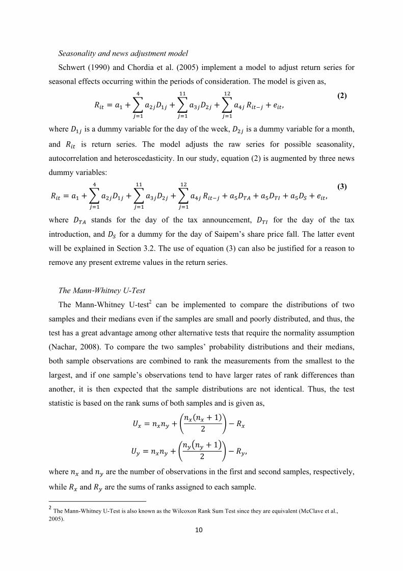
Seasonality and news adjustment model

Schwert (1990) and Chordia et al. (2005) implement a model to adjust return series for

seasonal effects occurring within the periods of consideration. The model is given as,

𝑅!" = 𝑎! + 𝑎!!𝐷!!

!

!!!

+ 𝑎!!𝐷!!

!!

!!!

+ 𝑎!!

!"

!!!

𝑅!"!! + 𝑒!" , (2)

where 𝐷!! is a dummy variable for the day of the week, 𝐷!! is a dummy variable for a month,

and 𝑅!" is return series. The model adjusts the raw series for possible seasonality,

autocorrelation and heteroscedasticity. In our study, equation (2) is augmented by three news

dummy variables:

𝑅!" = 𝑎! + 𝑎!!𝐷!!

!

!!!

+ 𝑎!!𝐷!!

!!

!!!

+ 𝑎!!

!"

!!!

𝑅!"!! + 𝑎!𝐷!" + 𝑎!𝐷!" + 𝑎!𝐷! + 𝑒!" , (3)

where 𝐷!" stands for the day of the tax announcement, 𝐷!" for the day of the tax

introduction, and 𝐷! for a dummy for the day of Saipem’s share price fall. The latter event

will be explained in Section 3.2. The use of equation (3) can also be justified for a reason to

remove any present extreme values in the return series.

The Mann-Whitney U-Test

The Mann-Whitney U-test2 can be implemented to compare the distributions of two

samples and their medians even if the samples are small and poorly distributed, and thus, the

test has a great advantage among other alternative tests that require the normality assumption

(Nachar, 2008). To compare the two samples’ probability distributions and their medians,

both sample observations are combined to rank the measurements from the smallest to the

largest, and if one sample’s observations tend to have larger rates of rank differences than

another, it is then expected that the sample distributions are not identical. Thus, the test

statistic is based on the rank sums of both samples and is given as,

𝑈! = 𝑛!𝑛! +𝑛! 𝑛! + 1

2 − 𝑅!

𝑈! = 𝑛!𝑛! +𝑛! 𝑛! + 1

2 − 𝑅! ,

where 𝑛! and 𝑛! are the number of observations in the first and second samples, respectively,

while 𝑅! and 𝑅! are the sums of ranks assigned to each sample.

2The Mann-Whitney U-Test is also known as the Wilcoxon Rank Sum Test since they are equivalent (McClave et al., 2005).

11

The Mann-Whitney U-Test’s null hypothesis states that the two samples come from

identical populations and that the medians of both samples are not different, while the

alternative hypothesis stipulates that the probability distribution of one sample shifted to the

left or to the right of another; hence, one sample’s median is larger than the other (Nachar,

2008; McClave et al., 2005). There are two main conditions that are required for the test to be

valid. First, the two investigated samples are random, independent and drawn from the same

population, and second, their probability distributions are continuous. Because it is not

expected for the series of liquidity measures considered in this paper to be normally

distributed and assuming that the series fit the abovementioned requirements, the Mann-

Whitney test is chosen to compare changes in liquidities of stocks.

Levene’s, Brown-Forsythe, and O’Brien Tests

We use a time series of logarithmic returns, residuals of equation (1) and equation (3) to

test for the difference in return volatility before and after tax announcement and introduction

events. The null hypothesis is that the variances of the two samples are equal. This approach

is also employed by Baltagi et al. (2006), where the homogeneity of variances of returns is

tested. There are several tests that can be implemented to examine the homogeneity of

variances of two samples. In our study, the following statistics are used.

Because the common F-ratio and Bartlett’s tests for equality of variances are very

sensitive to departures from the normality assumption, in 1960, Howard Levene developed

two different statistics and demonstrated their satisfactory power under non-normality

conditions (Levene, 1960). The two modifications of Levene’s tests employ the absolute and

quadratic measures, which are given as follows:

𝑊 = 𝑁 − 𝑘 𝑁! 𝑍! − 𝑍 !!

!!!

𝑘 − 1 (𝑍!"!!!!!

!!!! − 𝑍!) !

(5)

where 𝑁! is the sample size of the ith group and k is the number of groups, while the

definition of 𝑍!" differs depending on the variety of the test. For the absolute estimate, the test

statistic uses 𝑍!" = 𝑌!" − 𝑌! , where 𝑌! is the mean of the ith subgroup, 𝑍 is the mean of all

𝑍!", 𝑍! is the mean of 𝑍!" in subgroup i, while for the quadratic form, the test statistic uses

𝑍!"! = 𝑌!" − 𝑌! ! , where 𝑌! is the mean of the ith subgroup. Levene’s tests do not assume

the equality of means of investigated group samples (Baltagi et al., 2006). Critical values are

obtained from the Snedecor F-table (Brown and Forsythe, 1974).

12

However, Brown and Forsythe (1974) argue that the estimate of the mean in the Levene’s

test should be replaced by the median measure, which they prove to be a more robust

estimate. As a result, they define 𝑍!" in equation (5) as 𝑍!" = 𝑌!" − 𝑌! , where 𝑌! is the

median of the ith subgroup.

Another modification of Levene’s statistic is provided by O’Brien (1981). For this test

type, the test statistic in equation (5) uses

𝑍!" =!.!! !!!! !! !!"!!! ! !!.!(!!!!)!!

!

(!!!!)(!!!!),

where 𝑛! is the size of the ith group and 𝑠!! is the sample variance. Abdi (2007) states that

O’Brien’s test is versatile compared with other tests and minimises both the type I and type II

errors. In this study, we use both versions of the test. However, the preference in obtained

results is given to the modified test of Brown and Forsythe (1974) to be consistent with

Baltagi et al. (2006).

3.2 Data description

Analysed in this paper are closing spot, bid and ask prices of Italian shares that are traded

or used to trade in the Borsa Italiana, the Italian national stock exchange, with market

capitalisation of above 500 million Euros on 30 November 2012 and 28 February 2013.

Prices are obtained from Bloomberg and are denominated in Euros. Weekends and holidays

are excluded, resulting in 125 daily observations.

The six-month period from 29 October 2012 to 30 April 2013 is chosen to examine the

effect of the announcement and imposition of the FTT on liquidity and volatility of stock

returns by comparing two months prior to and two months after the events. A six-month

sample is divided into three equal subsamples: the period from the tax announcement event,

29 December 2012, to the tax introduction day, 1 March 2013, comprises two months, which

is used as both a post-announcement period as well as a pre-tax imposition period. Similar

short-term sample periods for detecting the effect of the financial tax on market efficiency are

used by Baltagi et al. (2006) and Colliard and Hoffmann (2015).

The Ministry of Economy and Finance of Italy introduced a list of exempt resident Italian

companies, the shares of which have a market capitalisation of less than 500 million Euros in

November 2012 (di Wiesenhoff and Egori, 2013) and in February 2013 (Coelho, 2015). We

compile a list of taxable shares using both November 2012 and February 2013 market

capitalisations. The former is employed for evaluating the effect of the tax announcement,

while the latter is used to study the effect of the tax imposition. There are 77 shares with

13

market capitalisation exceeding 500 million Euros on 30 November 2012, and there are 81

shares with market capitalisation of 500 million Euros or above as of 28 February 2013,

according to the Borsa Italiana.

To test for any effect of FTT on stock liquidity and volatility, all stocks are combined into

one joint portfolio and ten size-sorted (decile) portfolios weighted by market capitalisation of

November 2012 and February 2013. The joint portfolio is used to examine the effect of FTT,

if any, on all chosen stocks, while size-sorted decile portfolios are used to note any sensitivity

of the possible effect with respect to market capitalisation. The largest group by market

capitalisation is denoted as Portfolio 1 (decile 1) and the smallest as Portfolio 10 (decile 10).

Table 1 provides two lists of companies with a capitalisation of 500 million Euros or above

based on two dates and the companies’ corresponding weights. The weight of each share is

estimated as

wi = ci/ct,

where wi is a weight of individual share i in a portfolio, ci is individual share capitalisation

and ct is total sample capitalisation.

3.2.1 Bid and ask prices

Bid and ask prices are employed to extract two measures of liquidity following Chordia et

al. (2005). The obtained measures are the quoted spread measured as a difference between

bid and ask prices and the relative quoted spread measured as the quoted spread divided by

the mid-point of the bid-ask prices. Quoted and relative quoted spreads are estimated for each

stock and ordered by market capitalisation from the highest to the lowest according to the

November 2012 and February 2013 market capitalisations. To create liquidity measures for

the joint and size-sorted decile portfolios, the individual quoted and relative quoted spreads

are multiplied by the corresponding weights given in Table 1. As a result, 11 portfolios (one

joint and ten size-sorted) are generated from all stocks for each market capitalisation list.

Figure 1 plots the time series of quoted and relative quoted spreads of joint portfolios

based on two market capitalisation records (solid and dotted lines). Although weighted

differently, the joint portfolios based on two market capitalisation measures demonstrate

similar fluctuations throughout the period. Both panels A and B indicate that both liquidity

measures increase after the tax is imposed on 1 March 20133.

3Since the tax news was officially published on Saturday 29 December 2012 when the markets were closed until 4 January 2013, we take the previous day of 28 December as the pre-announcement sample end date. Our figures show 28 December as the announcement date for illustrative purposes only.

14

Table 1. List of shares issued by taxed Italian companies. The list is based on market capitalisations of November 2012 and February 2013. The portfolios are based on a weighted market capitalisation approach where weights are estimated as wi = ci/ct, where wi is the weight of an individual share in a portfolio, ci is individual share capitalisation and ct is total sample capitalisation. Each weighting scheme has one joint portfolio and 10 size-sorted decile portfolios. Portfolio 1 (P1) represents the decile portfolio with the largest market capitalisation, while Portfolio 10 (P10) is the decile portfolio with the smallest market capitalisation.

November 2012 market capitalisation February 2013 market capitalisation

Share

Market cap.,

million euro

Weights Share

Market cap.,

million euro

Weights

decile joint decile joint

Port

folio

1

1 ENI 66383.10 0.3377 0.1978 1 ENI 63251.62 0.3324 0.1864 2 ENEL 27568.17 0.1402 0.0822 2 ENEL 25921.21 0.1362 0.0764 3 UNICREDIT 20833.48 0.1060 0.0621 3 UNICREDIT 22493.09 0.1182 0.0663 4 GENERALI 20157.55 0.1025 0.0601 4 INTESA SANPAOLO 19247.92 0.1011 0.0567 5 INTESA SANPAOLO 20134.08 0.1024 0.0600 5 GENERALI 19186.48 0.1008 0.0565 6 SAIPEM 15143.11 0.0770 0.0451 6 LUXOTTICA GROUP 16646.67 0.0875 0.0490 7 LUXOTTICA GROUP 14849.02 0.0755 0.0443 7 SNAM 12242.39 0.0643 0.0361 8 SNAM 11518.94 0.0586 0.0343 8 FIAT INDUSTRIAL 11303.68 0.0594 0.0333

Total of decile 1 196587.45 Total of decile 1 190293.06

Port

folio

2

9 FIAT INDUSTRIAL 10098.95 0.1904 0.0301 9 SAIPEM 9044.08 0.1738 0.0266 10 TELECOM ITALIA 9412.11 0.1775 0.0281 10 ATLANTIA 8718.31 0.1676 0.0257 11 ATLANTIA 8691.42 0.1639 0.0259 11 TELECOM ITALIA 7529.88 0.1447 0.0222 12 ENEL GREEN POWER 6606.44 0.1246 0.0197 12 ENEL GREEN POWER 7025.89 0.1350 0.0207

13 TERNA 5871.15 0.1107 0.0175 13 TERNA 6396.85 0.1230 0.0188 14 FIAT 4425.27 0.0834 0.0132 14 FIAT 5073.25 0.0975 0.0149 15 PIRELLI & C 4247.02 0.0801 0.0127 15 PIRELLI & C 4229.24 0.0813 0.0125 16 MEDIOBANCA 3683.83 0.0695 0.0110 16 MEDIOBANCA 4009.54 0.0771 0.0118

Total of decile 2 53036.19 Total of decile 2 52027.04

Port

folio

3

17 TELECOM ITALIA RSP 3672.61 0.1467 0.0109 17 PRYSMIAN 3605.85 0.1340 0.0106 18 CAMPARI 3351.1 0.1339 0.0100 18 SALVATORE

FERRAGAMO 3535.5 0.1313 0.0104

19 PRYSMIAN 3133.5 0.1252 0.0093 19 CAMPARI 3519.28 0.1307 0.0104 20 PARMALAT 3119.68 0.1247 0.0093 20 EXOR 3417.78 0.1270 0.0101 21 EXOR 3044.58 0.1217 0.0091 21 TOD'S 3377.9 0.1255 0.0100 22 LOTTOMATICA 2930.64 0.1171 0.0087 22 PARMALAT 3208.18 0.1192 0.0095 23 SALVATORE

FERRAGAMO 2920.97 0.1167 0.0087 23 UBI BANCA 3136.82 0.1165 0.0092

24 TOD'S 2853.97 0.1140 0.0085 24 MEDIOLANUM 3115.93 0.1158 0.0092 Total of decile 3 25027.05 Total of decile 3 26917.24

Port

folio

4

25 MEDIOLANUM 2764.99 0.1593 0.0082 25 LOTTOMATICA 3057.51 0.1580 0.0090 26 UBI BANCA 2738.88 0.1578 0.0082 26 TELECOM ITALIA RSP 2961.48 0.1531 0.0087 27 BANCA MONTE PASCHI

SIENA 2370.48 0.1366 0.0071 27 AUTOGRILL 2470.35 0.1277 0.0073

28 FINMECCANICA 2346.16 0.1352 0.0070 28 BANCA MONTE PASCHI SIENA

2463.96 0.1273 0.0073

29 BANCO POPOLARE 2006.61 0.1156 0.0060 29 BANCO POPOLARE 2262.82 0.1170 0.0067 30 AUTOGRILL 1935.96 0.1116 0.0058 30 FINMECCANICA 2183.56 0.1129 0.0064 31 DIASORIN 1597.06 0.0920 0.0048 31 MEDIASET 1986.19 0.1027 0.0059 32 BANCA POP EMILIA

ROMAGNA 1594.71 0.0919 0.0048 32 BUZZI UNICEM 1962.69 0.1014 0.0058

Total of decile 4 17354.85 Total of decile 4 19348.56

Port

folio

5

33 BUZZI UNICEM 1545.98 0.1310 0.0046 33 GEMINA 1935.61 0.1408 0.0057 34 DE' LONGHI 1542.3 0.1307 0.0046 34 BANCA POP EMILIA

ROMAGNA 1825.19 0.1327 0.0054

35 SIAS 1518.7 0.1287 0.0045 35 DE' LONGHI 1771.58 0.1288 0.0052 36 MEDIASET 1508.28 0.1278 0.0045 36 AZIMUT HOLDING 1737.37 0.1263 0.0051 37 BANCA CARIGE 1494.53 0.1266 0.0045 37 BANCA POPOLARE

MILANO 1663.1 0.1209 0.0049

38 AZIMUT HOLDING 1448.01 0.1227 0.0043 38 EXOR PRV 1608.28 0.1170 0.0047 39 BANCA GENERALI 1394.28 0.1181 0.0042 39 SIAS 1605.5 0.1168 0.0047 40 HERA 1351.67 0.1145 0.0040 40 IMPREGILO 1604.82 0.1167 0.0047

Total of decile 5 11803.75 Total of decile 5 13751.45

15

Port

folio

6

41 BANCA POPOLARE SONDRIO

1350.21 0.1305 0.0040 41 HERA 1602.65 0.1377 0.0047

42 RECORDATI 1350.12 0.1305 0.0040 42 DIASORIN 1596.39 0.1372 0.0047 43 BANCA POPOLARE

MILANO 1329.83 0.1285 0.0040 43 RECORDATI 1579.18 0.1357 0.0047

44 A2A 1319.04 0.1275 0.0039 44 BANCA GENERALI 1524.08 0.1309 0.0045 45 IMPREGILO 1285.31 0.1242 0.0038 45 BANCA POPOLARE

SONDRIO 1441.11 0.1238 0.0042

46 EXOR PRV 1267.81 0.1225 0.0038 46 BANCA CARIGE 1396.4 0.1200 0.0041 47 CREDITO EMILIANO 1232.45 0.1191 0.0037 47 A2A 1298.82 0.1116 0.0038 48 GEMINA 1212.76 0.1172 0.0036 48 CREDITO EMILIANO 1200.03 0.1031 0.0035

Total of decile 6 10347.53 Total of decile 6 11638.66

Port

folio

7

49 ANSALDO STS 1092.43 0.1451 0.0033 49 ANSALDO STS 1179.74 0.1446 0.0035 50 INTESA SANPAOLO RSP 986.17 0.1310 0.0029 50 BRUNELLO

CUCINELLI 1059.56 0.1299 0.0031

51 BRUNELLO CUCINELLI 934.03 0.1241 0.0028 51 FONDIARIA - SAI 1058.9 0.1298 0.0031 52 DANIELI & C 931.38 0.1237 0.0028 52 ERG 1034.93 0.1269 0.0030 53 RCS MEDIAGROUP 924.15 0.1228 0.0028 53 INTESA SANPAOLO

RSP 988.19 0.1211 0.0029

54 SARAS 891.67 0.1185 0.0027 54 ACEA 975.68 0.1196 0.0029 55 CREDITO

BERGAMASCO 888.99 0.1181 0.0026 55 BENI STABILI 939.71 0.1152 0.0028

56 FONDIARIA - SAI 878.19 0.1167 0.0026 56 AMPLIFON 920.77 0.1129 0.0027 Total of decile 7 7527.01 Total of decile 7 8157.48

Port

folio

8

57 ACEA 853.98 0.1547 0.0025 57 SORIN 914.46 0.1415 0.0027 58 BENI STABILI 852.83 0.1544 0.0025 58 SARAS 829.52 0.1284 0.0024 59 ERG 810.71 0.1468 0.0024 59 DANIELI & C 825.36 0.1277 0.0024 60 SORIN 795.09 0.1440 0.0024 60 YOOX 809.95 0.1253 0.0024 61 AMPLIFON 777.47 0.1408 0.0023 61 ITALCEMENTI 784.09 0.1213 0.0023 62 PIAGGIO & C 717.81 0.1300 0.0021 62 ASTM 773.75 0.1197 0.0023 63 UNIPOL 713.85 0.1293 0.0021 63 UNIPOL 765.59 0.1185 0.0023

64 RCS MEDIAGROUP 759.89 0.1176 0.0022

Total of decile 8 5521.74 Total of decile 8 6462.61

Port

folio

9

64 YOOX 672.74 0.1493 0.0020 65 CREDITO BERGAMASCO

755.71 0.1361 0.0022

65 CIR 666.33 0.1479 0.0020 66 PIAGGIO & C 728.69 0.1312 0.0021 66 CATTOLICA

ASSICURAZIONI 663.30 0.1472 0.0020 67 CATTOLICA

ASSICURAZIONI 728.66 0.1312 0.0021

67 INDESIT COMPANY 638.31 0.1416 0.0019 68 BREMBO 708.38 0.1276 0.0021 68 ITALCEMENTI 633.30 0.1405 0.0019 69 MILANO

ASSICURAZIONI 683.01 0.1230 0.0020

69 ASTM 631.84 0.1402 0.0019 70 GEOX 654.92 0.1180 0.0019 70 BREMBO 600.61 0.1333 0.0018 71 INTERPUMP GROUP 652.95 0.1176 0.0019

72 INDESIT COMPANY 639.65 0.1152 0.0019 Total of decile 9 4506.43 Total of decile 9 5551.97

Port

folio

10

71 INTERPUMP GROUP 591.46 0.1547 0.0018 73 CAMFIN 637.16 0.1212 0.0019 72 MILANO

ASSICURAZIONI 571.06 0.1494 0.0017 74 IREN 623.63 0.1186 0.0018

73 EI TOWERS 570.15 0.1491 0.0017 75 CIR 618.29 0.1176 0.0018 74 GEOX 545.25 0.1426 0.0016 76 EI TOWERS 616.96 0.1173 0.0018 75 IMA 526.88 0.1378 0.0016 77 IMA 604.07 0.1149 0.0018 76 IREN 514.56 0.1346 0.0015 78 MARR 578.74 0.1101 0.0017 77 DANIELI & C RSP 504.12 0.1318 0.0015 79 ASTALDI 535.38 0.1018 0.0016

80 SAFILO GROUP 524.18 0.0997 0.0015 81 DANIELI & C RSP 520.27 0.0989 0.0015

Total of decile 10 3823.48 Total of decile 10 5258.68

Total market capitalisation 335535.48 Total market capitalisation 339406.75

Similarly, Figure 2 demonstrates relative quoted spreads of the decile portfolios based on

the February market capitalisation record. Like the spreads of joint portfolios, the spreads of

decile portfolios, regardless of the size, tend to increase after the introduction of the tax and

seem to demonstrate no effect of the announcement date. Furthermore, the figure shows that

the higher the market capitalisation of the portfolio (see decile portfolios P1-P4 in Figure 2),

16

the smaller the bid-ask spread on average, while portfolios with small market capitalisation

demonstrate much wider bid-ask spreads (see for example portfolios P6-P10 in Figure 2)4.

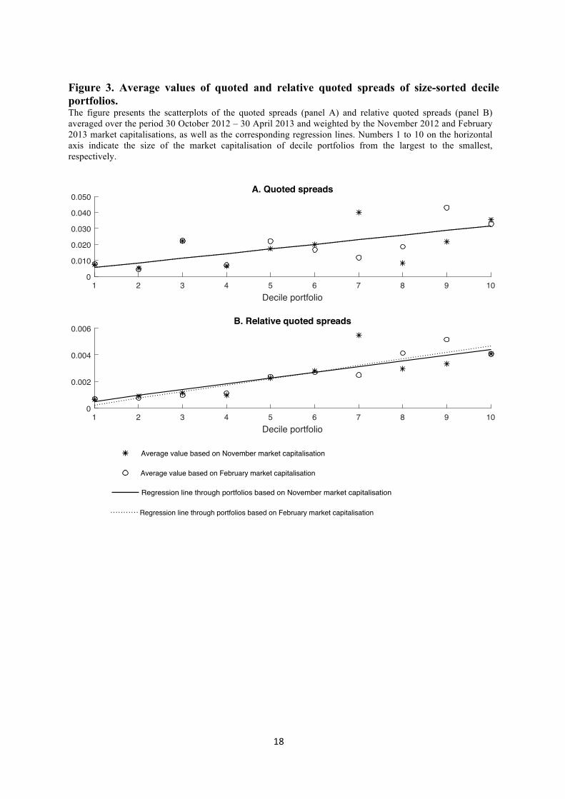
This observation is confirmed by Figure 3, which documents an upward tendency in the

quoted and relative quoted spreads averaged over the whole time period of six months for

each decile portfolio. Figure 3 shows that the higher the market capitalisation, the smaller the

bid-ask spread.

Figure 1. Quoted and relative quoted spreads of joint portfolios, October 2012 – April 2013, daily observations. The figure presents plots of quoted (panel A) and relative quoted spreads (panel B) based on orders of November 2012 and February 2013 market capitalisations. The date of the tax announcement is marked as 28 December because the tax news was published on Saturday 29 December when the markets were closed.

4Figures of quoted spreads of the February market capitalisation, as well as of both liquidity measures based on the November capitalisation are similar. They are omitted for brevity and are available from authors upon request.

29/10/12 28/12/12 01/03/13 30/04/130

0.005

0.01

0.015

0.02A. Quoted spreads

29/10/12 28/12/12 01/03/13 30/04/130

0.5

1

1.5

2 �10-3 B. Relative quoted spreads

February market capitalisationNovember market capitalisation

17

Figure 2. Relative quoted spreads of size-sorted decile portfolios (February market cap). The figure presents the plots of size-sorted decile portfolios for relative quoted spreads based on February 2013 market capitalisation. P1 and P10 stand for the largest and the smallest decile portfolio by market capitalisation, respectively.

Using 11 portfolios (one joint and ten decile portfolios) for both liquidity measures and

both market capitalisations, Table 2 provides the summary statistics of the series. In addition

to confirming the graphical evidence about the average liquidity values across decile

portfolios, relative quoted spreads of all portfolios have lower variations than those of the

quoted spread series because the means and standard deviations of the former series are

several times lower than those of the latter series. The skewness and kurtosis of all series of

spreads clearly deviate from those of the normal distribution, and the Jarque-Bera (JB) tests

confirm that the series are not normally distributed by rejecting the null hypothesis of

normality at a less than 10% significance level. Another test of the Ljung-Box for an up-to-

22-order serial correlation indicates that most of the series are autocorrelated, where the null

hypothesises of no serial correlations is rejected at a less than 10% significant level.

29/10/12 28/12/12 01/03/13 30/04/130

0.002

P1

29/10/12 28/12/12 01/03/13 30/04/130

0.002

P2

29/10/12 28/12/12 01/03/13 30/04/130

0.002

P3

29/10/12 28/12/12 01/03/13 30/04/130

0.004

P4

29/10/12 28/12/12 01/03/13 30/04/130

0.005

P5

29/10/12 28/12/12 01/03/13 30/04/130

0.010

P6

29/10/12 28/12/12 01/03/13 30/04/130

0.010

P7

29/10/12 28/12/12 01/03/13 30/04/130

0.010

P8

29/10/12 28/12/12 01/03/13 30/04/130

0.010

P9

29/10/12 28/12/12 01/03/13 30/04/130

0.010

P10

18

Figure 3. Average values of quoted and relative quoted spreads of size-sorted decile portfolios. The figure presents the scatterplots of the quoted spreads (panel A) and relative quoted spreads (panel B) averaged over the period 30 October 2012 – 30 April 2013 and weighted by the November 2012 and February 2013 market capitalisations, as well as the corresponding regression lines. Numbers 1 to 10 on the horizontal axis indicate the size of the market capitalisation of decile portfolios from the largest to the smallest, respectively.

1 2 3 4 5 6 7 8 9 10Decile portfolio

0

0.010

0.020

0.030

0.040

0.050A. Quoted spreads

Average value based on November market capitalisationRegression line through portfolios based on November market capitalisationAverage value based on February market capitalisationRegression line through portfolios based on February market capitalisation

1 2 3 4 5 6 7 8 9 10Decile portfolio

0

0.002

0.004

0.006B. Relative quoted spreads

1 2 3 4 5 6 7 8 9 10Decile portfolio

0

0.01

0.02

0.03

0.04

0.05A. Quoted spreads

Average value based on November market capitalisationRegression line through portfolios based on November market capitalisation

1 2 3 4 5 6 7 8 9 10Decile portfolio

0

0.001

0.002

0.003

0.004

0.005

0.006B. Relative Quoted spreads

Average value based on February market capitalisationRegression line through portfolios based on February market capitalisation

1 2 3 4 5 6 7 8 9 10Decile portfolio

0

0.01

0.02

0.03

0.04

0.05A. Quoted spreads

Average value based on November market capitalisationRegression line through portfolios based on November market capitalisation

1 2 3 4 5 6 7 8 9 10Decile portfolio

0

0.001

0.002

0.003

0.004

0.005

0.006B. Relative Quoted spreads

Average value based on February market capitalisationRegression line through portfolios based on February market capitalisation

1 2 3 4 5 6 7 8 9 10Decile portfolio

0

0.01

0.02

0.03

0.04

0.05A. Quoted spreads

Average value based on November market capitalisationRegression line through portfolios based on November market capitalisation

1 2 3 4 5 6 7 8 9 10Decile portfolio

0

0.001

0.002

0.003

0.004

0.005

0.006B. Relative Quoted spreads

Average value based on February market capitalisationRegression line through portfolios based on February market capitalisation

1 2 3 4 5 6 7 8 9 10Decile portfolio

0

0.01

0.02

0.03

0.04

0.05A. Quoted spreads

Average value based on November market capitalisationRegression line through portfolios based on November market capitalisation

1 2 3 4 5 6 7 8 9 10Decile portfolio

0

0.001

0.002

0.003

0.004

0.005

0.006B. Relative Quoted spreads

Average value based on February market capitalisationRegression line through portfolios based on February market capitalisation

19

Table 2. Summary statistics of the time series of liquidity measures, November 2012 and February 2013 market capitalisation records, October 2012 – April 2013, 125 daily observations. The table presents summary statistics for the quoted spreads (QS) and relative quoted spreads (RQS) for the joint and decile portfolios.

November 2012 market capitalisation February 2013 market capitalisation

P Variable Mean Standard Deviation Skewness Kurtosis Jarque-Berra Q(22) Mean Standard

Deviation Skewness Kurtosis Jarque-Berra Q(22)

Joint QS 0.010 0.007 -9.149 96.912 47678.19 (0.00) 12.21 (0.95) 0.011 0.005 -6.512 64.601 20647.40 (0.00) 68.05 (0.00) RQS 0.001 0.000 -3.274 27.991 3476.20 (0.00) 260.97 (0.00) 0.001 0.000 -0.934 8.994 205.26 (0.00) 520.94 (0.00)

1 QS 0.007 0.012 -10.471 114.953 67562.72 (0.00) 0.68 (1.00) 0.008 0.002 2.931 14.386 854.15 (0.00) 34.26 (0.05) RQS 0.001 0.001 -10.426 114.317 66803.08 (0.00) 0.65 (1.00) 0.001 0.000 2.565 11.866 546.49 (0.00) 32.92 (0.06)

2 QS 0.005 0.001 1.342 4.600 50.87 (0.00) 65.85 (0.00) 0.004 0.024 -10.943 121.520 75656.64 (0.00) 0.40 (1.00) RQS 0.001 0.000 1.288 4.432 45.23 (0.00) 105.38 (0.00) 0.001 0.002 -10.878 120.582 74472.87 (0.00) 0.24 (1.00)

3 QS 0.022 0.011 2.301 10.460 400.22 (0.00) 341.65 (0.00) 0.022 0.011 2.454 11.546 505.89 (0.00) 299.96 (0.00) RQS 0.001 0.000 2.341 10.789 430.17 (0.00) 216.80 (0.00) 0.001 0.001 2.511 11.974 550.80 (0.00) 183.06 (0.00)

4 QS 0.006 0.002 1.332 4.385 46.94 (0.00) 112.43 (0.00) 0.007 0.003 1.780 6.439 127.59 (0.00) 273.82 (0.00) RQS 0.001 0.000 1.239 3.948 36.66 (0.00) 186.45 (0.00) 0.001 0.001 1.734 6.458 124.90 (0.00) 284.03 (0.00)

5 QS 0.018 0.006 0.822 4.096 20.33 (0.00) 61.73 (0.00) 0.022 0.009 1.210 5.244 56.71 (0.00) 81.51 (0.00) RQS 0.002 0.001 0.730 3.758 14.08 (0.00) 83.01 (0.00) 0.003 0.001 1.021 4.920 40.92 (0.00) 30.14 (0.12)

6 QS 0.020 0.010 1.061 4.134 30.15 (0.00) 215.85 (0.00) 0.017 0.007 1.103 4.686 40.17 (0.00) 195.28 (0.00) RQS 0.004 0.002 0.939 4.019 23.76 (0.00) 109.00 (0.00) 0.002 0.001 1.079 4.584 37.34 (0.00) 228.66 (0.00)

7 QS 0.040 0.018 0.535 3.119 6.04 (0.05) 59.55 (0.00) 0.012 0.005 1.142 4.473 38.49 (0.00) 101.89 (0.00) RQS 0.006 0.003 0.545 3.180 6.37 (0.04) 73.18 (0.00) 0.002 0.001 0.972 4.075 25.70 (0.00) 64.12 (0.00)

8 QS 0.008 0.004 0.898 3.177 16.98 (0.00) 326.33 (0.00) 0.018 0.009 1.038 3.692 24.93 (0.00) 278.51 (0.00) RQS 0.003 0.001 0.813 3.192 13.97 (0.00) 241.01 (0.00) 0.003 0.001 0.997 3.683 23.14 (0.00) 242.73 (0.00)

9 QS 0.022 0.010 1.194 4.131 36.37 (0.00) 252.82 (0.00) 0.043 0.019 0.555 2.825 6.57 (0.04) 81.35 (0.00) RQS 0.003 0.001 1.124 4.103 32.67 (0.00) 116.62 (0.00) 0.007 0.003 0.596 2.907 7.43 (0.02) 82.35 (0.00)

10 QS 0.035 0.018 1.562 5.475 82.71 (0.00) 294.37 (0.00) 0.033 0.015 1.765 6.945 145.97 (0.00) 333.96 (0.00) RQS 0.004 0.002 1.520 5.519 81.18 (0.00) 193.51 (0.00) 0.004 0.001 1.104 4.163 32.43 (0.00) 568.29 (0.00)

20

3.2.2 Spot prices

We use the closing prices of stocks to obtain three measures of return time series to test

them for possible volatility changes around the tax announcement and tax imposition dates.

For this reason, motivated by Baltagi et al. (2006), Hu (1998) and Chordia et al. (2005), three

series are respectively estimated, namely logarithmic returns, residuals of equation (1) and

residuals of equation (3).

Individual logarithmic return series are calculated as continuously compounded daily

returns:

rt = ln(pt/pt-1)*100%,

where pt and pt-1 are stock prices at time t and t-1, respectively, and ln is the natural

logarithm.

Logarithmic returns of joint and size-sorted decile portfolios are calculated as weighted

average returns where the weights correspond to the market capitalisation records given in

Table 1. As a result, 11 portfolio return series, including one joint and ten decile portfolios,

are obtained for the November 2012 and February 2013 market capitalisations.

Table 3. Market model regressions.

The table provides results of the market model regressions represented by equation (1) using excess returns of joint portfolios, the largest (P1) and smallest (P10) decile portfolios for both market capitalisations. Regressions are adjusted for possible autocorrelation and heteroscedasticity in the residuals using Newey-West procedure. Standard errors are in italics in parentheses. ***, ** and * indicate statistical significance at the 10%, 5% and 1% levels, respectively.

Variables Excess returns, joint portfolio Excess returns, decile portfolio P1 Excess returns, decile portfolio P10

November cap February cap November cap February cap November cap February cap

Intercept

Excess market return

-0.001

(0.01)

0.967*

(0.01)

0.017* (0.01)

0.954* (0.00)

-0.033 (0.03)

1.060* (0.03)

0.006 (0.02)

1.037* (0.02)

0.158** (0.07)

0.664* (0.04)

0.182** (0.07)

0.598* (0.04)

Adj R2: Residual

diagnostics: Q(12)

JB Obs*R2

0.99

11.01 (0.53)

679.13 (0.00) 12.92 (0.00)

0.997

17.61 (0.13) 2.06 (0.37) 0.73 (0.69)

0.96

15.62 (0.21)

873.29 (0.00) 14.08 (0.00)

0.97

16.33 (0.18) 49.93 (0.00) 6.17 (0.05)

0.65

9.85 (0.63) 6.50 (0.04) 0.87 (0.65)

0.58

14.62 (0.26) 2.03 (0.36) 0.13 (0.94)

Note: P-values are in parentheses for the residual diagnostics.

21

Table 3 presents the results of estimating equation (1) for one joint portfolio, the largest

decile portfolio and the smallest decile portfolio5 for two market capitalisation records. The

FTSE Italian All Shares Index is used as a proxy for the market return variable in the market

model, while the risk-free rate is represented by the US one-month Treasury Bill. The excess

return on the market proxy shows highly significant explanatory power for the variability of

all excess returns of the given portfolios. Residuals from these regressions will be employed

for subsequent testing. Although the residuals do not show serial correlation at any

significance level less than 10%, as demonstrated by the Ljung-Box test statistics for an up-

to-22-order serial correlation, they deviate from the normality in about two-thirds of the

cases.

Regression results and residual diagnostics for equation (3) are presented in Table 4.

Because none of the coefficients on the day of the week dummy variables are significant

across all regressions, they are omitted from the regressions. The month of February has a

negative and statistically significant impact at a less than 5% level on the returns of joint

portfolios and large market capitalisation portfolio P1, while it causes no impact on the small

capitalisation portfolio P10. January, in contrast, positively affects the small capitalisation

portfolio, but not the large one or the joint one. Interestingly, coefficients on the tax

announcement dummy variables are positive and statistically significant at a less than 1%

level, while coefficients on the tax imposition event are negative and highly statistically

significant. The coefficient on a dummy variable for the Saipem share price drop is negative

as expected and is highly significant in all regression specifications. Regression residuals

show no signs of serial correlation and are normally distributed.

Figure 4 plots the time series of three return measures for joint portfolios based on two

market capitalisation records: the logarithmic returns on Panel A, residuals of the market

model in Panel B and residuals of the adjusted model in Panel C. In Panel A, there is an

abrupt return plunge on 30 January 2013, when the Saipem’s6 share price dropped by 34.3%,

resulting in other stocks tumbling, which knocked down Italy’s stock market (Stevenson,

2013). The overall tendency of the joint portfolio returns in Panel A, despite the difference in

weights, shows similar fluctuations throughout the period, indicating no sign of changes in

return variations among three subsample periods. Panel B plots the residuals of equation (1),

or market model residuals. A dramatic plunge on 30 January remains the lowest for the

5Regression results for the other decile portfolios are available from the authors upon request. 6Italian oil services group.

22

residuals based on the November capitalisation. However, for the February capitalisation

record, the fitted return is very close to the actual return on 30 January, resulting in a small

residual value. Both series will be employed for testing, and the difference between the two

will be noted. Panel C plots the residuals of the adjustment regression (3). Adjusting the

return series shows lower variations throughout the period compared with those of the raw

return series. Overall, the plots do not demonstrate any noticeable changes in variations

between pre- and post-FTT announcement and imposition days.

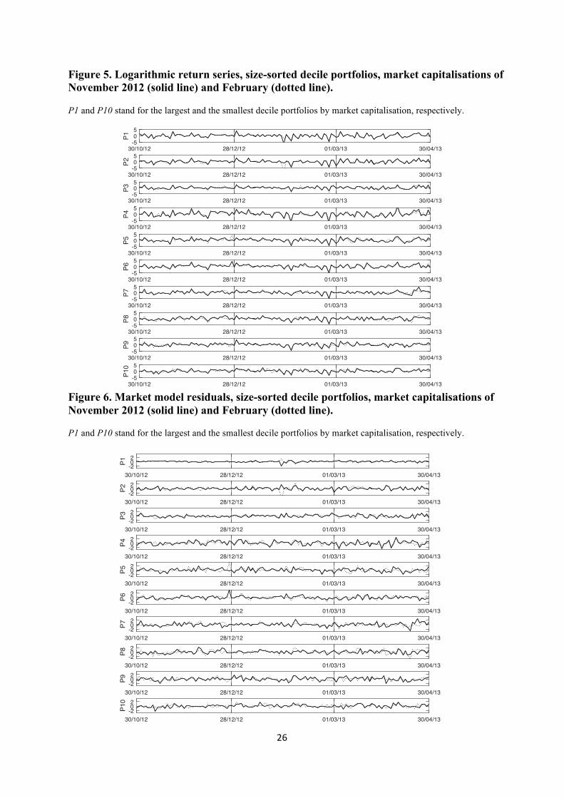
Figures 5, 6 and 7 illustrate three return measures of size-sorted decile portfolios for both

market capitalisation records. All graphs show no distinguishable changes in variations

between pre- and post-announcement or tax introduction periods.

The summary statistics of the logarithmic return series and residuals of equations (1) and

(3) for the joint and decile portfolios based on two market capitalisation records are presented

in Table 57. The logarithmic returns of the decile portfolios are mainly not normally

distributed as expected, except for portfolios P3, P4 and P10 of the February market

capitalisation. Residuals of the market model are normally distributed for 12 out of 20 cases

without any discernible pattern across portfolios. For the adjusted residuals, portfolios with

medium capitalisation tend to be non-normal (P4-P9 for the November capitalisation, P5-P8

for the February capitalisation). Ljung-Box test statistics for an up-to-22-order serial

correlation for all but three portfolio returns do not reject the null hypothesis of no

autocorrelation at the 10% significance level.

7There are 22 portfolios in total: two joint portfolios and 20 decile portfolios for each return measure: one half is based on the November market capitalisation, and the other half is based on the February market capitalisation.

23

Table 4. Adjustment regressions.

The table provides the results of estimating equation (3) using a return series of joint portfolios, the largest and smallest decile portfolios based on the November and February market capitalisations. Regressions are adjusted for possible autocorrelation and heteroscedasticity in the residuals using Newey-West procedure. Standard errors are in italics in parentheses. ***, ** and * indicate statistical significance at the 10%, 5% and 1% levels, respectively.

Variables Log return,

joint portfolio Log returns,

decile portfolio P1 Log returns,

decile portfolio P10 November cap February cap November cap February cap November cap February cap

Intercept

November

December

January

February

March

April

FTT announcement

FTT imposition

30 Jan 2013 (Saipem)

AR(1)

AR(3)

AR(8)

AR(12)

0.271 (0.21)

-

-0.098 (0.31) 0.150 (0.25)

-0.712** (0.33) -0.335 (0.31) 0.092 (0.38)

2.653* (0.27)

-1.258* (0.25)

-4.443* (0.14)

-0.189**

(0.09)

0.274 (0.21)

-

-0.064 (0.30) 0.174 (0.25)

-0.680** (0.33) -0.354 (0.31) 0.098 (0.38)

2.569* (0.27)

-1.235* (0.25)

-3.700* (0.14)

-0.192**

(0.10)

0.401*** (0.24)

-

-0.185 (0.34) 0.072 (0.27)

-1.006** (0.41) -0.584 (0.38) 0.086 (0.43)

2.819* (0.29)

-0.977* (0.32)

-3.017* (0.18)

-0.191* (0.07)

-0.194** (0.10)

0.386 (0.23)

-

-0.270 (0.35) -0.001 (0.26)

-1.002* (0.38) -0.462 (0.37) 0.041 (0.43)

2.995* (0.26)

-0.934* (0.31)

-6.115* (0.16)

-0.166** (0.07)

-0.179** (0.09)

0.068* (0.01)

-0.152 (0.27) 0.142 (0.25) 0.536* (0.13) -0.142 (0.27) 0.134 (0.17) 0.420 (0.26)

1.763* (0.13)

-0.466* (0.17)

-3.507* (0.13)

0.138 (0.27)

-

0.039 (0.31) 0.284 (0.37) -0.119 (0.36) 0.076 (0.35) 0.187 (0.40)

1.804* (0.26)

-1.344* (0.30)

-2.716* (0.27)

0.159 (0.11) 0.125 (0.11)

R2

Residual diagnostics:

Q(12) JB

Obs*R2

0.22

10.91 (0.54) 3.84 (0.15)

27.53 (0.02)

0.20

10.79 (0.55) 4.50 (0.11)

29.52 (0.01)

0.22

9.60 (0.65) 4.52 (0.10)

34.30 (0.06)

0.29

8.80 (0.72) 2.77 (0.25)

29.32 (0.17)

0.15

6.56 (0.89) 2.06 (0.36) 9.42 (0.40)

0.17

10.20 (0.60) 0.48 (0.79)

22.62 (0.48) Note: P-values are in parentheses for the residual diagnostics.

24

Figure 4. Plots of three return series of the joint portfolios based on the November 2012 and February 2013 market capitalisations, October 2012 – April 2013, 125 daily observations. The figure plots portfolio returns as the logarithmic returns (panel A), market model residuals (panel B) and adjusted residuals (panel C). The adjusted series lose the first few observations due to the lag component of equation (3). The date of the tax announcement is marked as 28 December for illustrative purposes because the tax news was published on Saturday 29 December when the markets were closed.

30/10/12 28/12/12 01/03/13 30/04/13-4.0

2.0

0

2.0%

A. Logarithmic returns

30/10/12 28/12/12 01/03/13 30/04/13-0.4

-0.2

0

0.2%

B. Market model residuals

30/10/12 28/12/12 01/03/13 30/04/13-4.0

-2.0

0

2.0%

C. Adjusted residuals

February market capitalisationNovember market capitalisation

25

Table 5. The summary statistics of the logarithmic returns, market model residuals and adjusted return residuals, October 2012 – April 2013, daily observations. R stands for logarithmic returns, MM for residuals of the market model and ADJ for residuals of the adjusted equation. P-values are in parentheses for the Jarque-Berra and Q-tests.

Market capitalisation of November 2012 Market capitalisation of February 2013

P Variable Mean Standard Deviation Skewness Kurtosis Jarque-Berra Q(22) Mean Standard

Deviation Skewness Kurtosis Jarque-Berra Q(22)

Joint R 0.069 1.319 -0.534 4.677 20.41 (0.00) 28.10 (0.17) 0.086 1.299 -0.497 4.574 17.90 (0.00) 27.93 (0.18) MM 0.000 0.104 -1.670 13.968 679.13 (0.00) 18.39 (0.68) 0.000 0.076 0.207 3.477 2.06 (0.36) 38.81 (0.02) ADJ 0.000 1.191 -0.243 3.767 3.84 (0.15) 22.57 (0.43) 0.000 1.189 -0.273 3.817 4.50 (0.11) 22.63 (0.42)

1 R 0.044 1.474 -0.639 5.048 30.10 (0.00) 27.67 (0.19) 0.081 1.434 -0.455 4.330 13.42 (0.00) 28.91 (0.15) MM 0.000 0.306 -2.136 15.279 873.29 (0.00) 21.43 (0.49) 0.000 0.266 0.179 6.088 49.93 (0.00) 21.32 (0.50) ADJ 0.000 1.267 -0.300 3.484 2.77 (0.25) 15.42 (0.84) 0.000 1.296 -0.401 3.569 4.52 (0.10) 17.11 (0.76)

2 R 0.057 1.329 -0.410 4.386 13.39 (0.00) 32.90 (0.06) -0.011 1.465 -1.516 10.600 345.96 (0.00) 23.35 (0.38) MM 0.000 0.596 0.187 3.394 1.52 (0.47) 27.04 (0.21) 0.000 0.750 -2.170 19.472 1499.13 (0.00) 20.99 (0.52) ADJ 0.000 1.248 -0.219 3.563 2.38 (0.30) 22.97 (0.40) 0.000 1.178 -0.015 3.093 0.05 (0.98) 23.24 (0.39)

3 R 0.105 0.992 0.183 3.448 1.73 (0.42) 20.91 (0.53) 0.145 1.181 -0.032 3.787 3.22 (0.20) 17.44 (0.74) MM 0.000 0.571 0.286 2.925 1.72 (0.42) 16.72 (0.78) 0.000 0.544 0.327 3.143 2.32 (0.31) 18.80 (0.66) ADJ 0.000 0.957 0.070 3.333 0.61 (0.74) 21.93 (0.46) 0.000 1.107 -0.074 3.767 2.84 (0.24) 17.65 (0.73)

4 R 0.089 1.929 -0.093 4.090 6.32 (0.04) 16.53 (0.79) 0.072 1.606 -0.053 3.846 3.76 (0.15) 24.89 (0.30) CAPM 0.000 0.918 -0.230 3.469 2.23 (0.33) 16.02 (0.82) 0.000 0.771 0.144 2.929 0.45 (0.80) 15.56 (0.84) ADJ 0.000 1.812 -0.091 4.013 5.47 (0.06) 19.26 (0.63) 0.000 1.514 0.020 3.729 2.62 (0.27) 24.52 (0.32)

5 R 0.143 1.385 -0.450 4.094 10.37 (0.01) 19.97 (0.59) 0.242 1.372 -0.150 4.151 7.30 (0.03) 9.78 (0.99) MM 0.000 0.767 -0.248 3.114 1.33 (0.51) 16.73 (0.78) 0.000 0.776 0.961 6.504 82.51 (0.00) 21.74 (0.48) ADJ 0.000 1.310 -0.234 3.912 5.43 (0.07) 19.04 (0.64) 0.000 1.327 -0.003 4.252 8.10 (0.02) 16.89 (0.77)

6 R 0.223 1.342 -0.390 4.691 17.91 (0.00) 12.64 (0.94) 0.112 1.237 -0.550 5.600 41.18 (0.00) 18.21 (0.69) MM 0.000 0.610 0.881 5.906 59.68 (0.00) 23.25 (0.39) 0.000 0.651 0.004 3.378 0.74 (0.69) 30.67 (0.10) ADJ 0.000 1.269 -0.299 4.645 15.83 (0.00) 19.63 (0.61) 0.000 1.143 -0.438 4.939 23.37 (0.00) 14.86 (0.87)

7 R 0.108 1.231 -0.294 5.682 38.93 (0.00) 12.74 (0.94) 0.176 1.165 -0.608 5.099 30.40 (0.00) 13.90 (0.91) MM 0.000 0.790 -0.014 4.412 10.30 (0.01) 20.59 (0.55) 0.000 0.669 0.119 3.536 1.78 (0.41) 22.07 (0.46) ADJ 0.000 1.178 -0.301 5.129 25.30 (0.00) 16.67 (0.78) 0.000 1.103 -0.462 5.002 25.11 (0.00) 13.75 (0.91)

8 R 0.164 1.175 -0.500 4.002 10.36 (0.01) 9.47 (0.99) 0.130 1.250 -0.542 3.316 6.59 (0.04) 10.41 (0.98) MM 0.000 0.732 0.397 3.059 3.27 (0.19) 21.20 (0.51) 0.000 0.857 -0.418 4.719 18.89 (0.00) 10.81 (0.98) ADJ 0.000 1.111 -0.428 3.980 8.76 (0.01) 10.45 (0.98) 0.000 1.205 -0.539 3.437 7.00 (0.03) 11.76 (0.96)

9 R 0.162 1.183 -0.319 4.836 19.52 (0.00) 13.48 (0.92) 0.152 1.173 -0.288 4.326 10.80 (0.00) 22.49 (0.43) MM 0.000 0.786 -0.097 2.787 0.43 (0.81) 15.64 (0.83) 0.000 0.693 0.218 2.943 1.00 (0.61) 22.09 (0.46) ADJ 0.000 1.098 -0.579 4.330 16.07 (0.00) 16.70 (0.78) 0.000 1.029 -0.316 3.611 3.80 (0.15) 21.76 (0.47)

10 R 0.207 1.116 -0.441 3.688 6.46 (0.04) 11.10 (0.97) 0.227 1.063 -0.106 3.450 1.28 (0.53) 23.31 (0.39) MM 0.000 0.656 -0.089 4.108 6.50 (0.04) 13.67 (0.91) 0.000 0.686 0.291 2.767 2.03 (0.36) 18.63 (0.67) ADJ 0.000 1.029 -0.276 3.306 2.06 (0.36) 12.06 (0.96) 0.000 0.982 0.157 3.013 0.48 (0.79) 20.36 (0.56)

26

Figure 5. Logarithmic return series, size-sorted decile portfolios, market capitalisations of November 2012 (solid line) and February (dotted line). P1 and P10 stand for the largest and the smallest decile portfolios by market capitalisation, respectively.

Figure 6. Market model residuals, size-sorted decile portfolios, market capitalisations of November 2012 (solid line) and February (dotted line). P1 and P10 stand for the largest and the smallest decile portfolios by market capitalisation, respectively.

30/10/12 28/12/12 01/03/13 30/04/13-505

P1

30/10/12 28/12/12 01/03/13 30/04/13-505

P2

30/10/12 28/12/12 01/03/13 30/04/13-505

P3

30/10/12 28/12/12 01/03/13 30/04/13-505

P4

30/10/12 28/12/12 01/03/13 30/04/13-505

P5

30/10/12 28/12/12 01/03/13 30/04/13-505

P6

30/10/12 28/12/12 01/03/13 30/04/13-505

P7

30/10/12 28/12/12 01/03/13 30/04/13-505

P8

30/10/12 28/12/12 01/03/13 30/04/13-505

P9

30/10/12 28/12/12 01/03/13 30/04/13-505

P10

30/10/12 28/12/12 01/03/13 30/04/13-202

P1

30/10/12 28/12/12 01/03/13 30/04/13-202

P2

30/10/12 28/12/12 01/03/13 30/04/13-202

P3

30/10/12 28/12/12 01/03/13 30/04/13-202

P4

30/10/12 28/12/12 01/03/13 30/04/13-202

P5

30/10/12 28/12/12 01/03/13 30/04/13-202

P6

30/10/12 28/12/12 01/03/13 30/04/13-202

P7

30/10/12 28/12/12 01/03/13 30/04/13-202

P8

30/10/12 28/12/12 01/03/13 30/04/13-202

P9

30/10/12 28/12/12 01/03/13 30/04/13-202

P10

27

Figure 7. Adjusted returns, size-sorted decile portfolios, market capitalisations of November 2012 (solid line) and February (dotted line). P1 and P10 stand for the largest and the smallest decile portfolios by market capitalisation, respectively.

4 Empirical results

In this section, the results of the test concerning the liquidity change around the tax

announcement and tax imposition events for the portfolios comprised of Italian stocks are

reported. The obtained results regarding volatility effect are introduced separately for each

series, namely, logarithmic returns, market model residuals and adjusted returns. The effect

of the tax announcement of 29 December 2012 is evaluated using the November

capitalisation since the February 2013 capitalisation cannot be known in December 2012. The

impact of the tax imposition event of 1 March 2013 is studied from the perspective of the

nearest market capitalisation of February 2013.

4.1 Liquidity

Using the method in section 3.1, quoted and relative quoted measures of the joint and

decile portfolios are tested for changes in their medians as a consequence of the tax

announcement and tax imposition. Table 6 presents the Mann-Whitney test results for two

joint portfolios. For completeness, test statistics for homogeneity of variances are also

included in the table.

30/10/12 28/12/12 01/03/13 30/04/13-505

P1

30/10/12 28/12/12 01/03/13 30/04/13-505

P2

30/10/12 28/12/12 01/03/13 30/04/13-505

P3

30/10/12 28/12/12 01/03/13 30/04/13-505

P4

30/10/12 28/12/12 01/03/13 30/04/13-505

P5

30/10/12 28/12/12 01/03/13 30/04/13-505

P6

30/10/12 28/12/12 01/03/13 30/04/13-505

P7

30/10/12 28/12/12 01/03/13 30/04/13-505

P8

30/10/12 28/12/12 01/03/13 30/04/13-505

P9

30/10/12 28/12/12 01/03/13 30/04/13-505

P10

28

Table 6. Test statistics for two liquidity measures of joint portfolios around the tax announcement, 29 December 2012, and tax imposition dates, 1 March 2013, daily observations, October 2012 – April 2013. ***, ** and * indicate statistical significance at 10%, 5% and 1%, respectively.

Statistic Quoted spreads Relative quoted spreads

A. Tax announcement, 29 December 2012, November market capitalisation Median before the event 0.0097 0.0011 Median after the event 0.0089 0.0009 Mann-Whitney U-test 2043* 2378* Standard Deviation before 0.011 0.000 Standard Deviation after 0.001 0.000 Levene’s absolute 2.184 1.207 Levene’s quadratic 1.052 1.052 Brown-Forsythe 1.090 1.302 O'Brien 1.029 1.026 B. Tax imposition, 1 March 2013, February market capitalisation Median before the event 0.0091 0.0009 Median after the event 0.0128 0.0014 Mann-Whitney U-test 970 * 926* Standard Deviation before 0.001 0.000 Standard Deviation after 0.002 0.000 Levene’s absolute 9.661* 2.366 Levene’s quadratic 5.408** 1.278 Brown-Forsythe 6.061** 2.541 O'Brien 5.275** 1.250

Table 6 Panel A demonstrates that the median quoted and relative quoted spread values

decrease from 0.0097 to 0.0089 and from 0.0011 to 0.0009 after the tax announcement date

of 29 December 2012 at the less than 1% significance level, suggesting that liquidity of the

affected Italian stocks increases after the FTT announcement. In contrast, Panel B shows that

the median quoted and relative quoted spreads increase after the tax introduction from 0.0091

to 0.0128 and 0.0009 to 0.0014 at the less than 1% statistically significant level, indicating

that liquidity of the affected stocks decreases after the tax imposition. The size of the

statistically significant increase in spreads ranges between 41% and 56%. Interestingly, the

volatility of quoted spreads almost doubles as a result of FTT imposition of 1 March 2013 at

the less than 5% significance level. However, there is no statistically significant difference

between volatility of liquidity measures around the tax announcement date.

29

Table 7. Mann-Whitney U-test statistics for quoted and relative quoted spreads of decile portfolios around the tax announcement and the tax imposition dates. P-values are in parentheses. ***, ** and * denote statistical significance at the 10%, 5% and 1% levels, respectively.

P Statistic Quoted spreads Relative quoted spreads

A. Tax announcement, 29 December 2012, November market capitalisation Median before 0.0076 0.0006 1 Median after 0.0074 0.0006 Mann-Whitney U-test 1903 (0.10)*** 1993 (0.06)*** Median before 0.0045 0.0008 2 Median after 0.0041 0.0007 Mann-Whitney U-test 1841.5 (0.28) 2251 (0.00)* Median before 0.0146 0.0007 3 Median after 0.0183 0.0008 Mann-Whitney U-test 1509.5 (0.01)* 1597 (0.09)*** Median before 0.0053 0.0008 4 Median after 0.0048 0.0006 Mann-Whitney U-test 1941 (0.16) 2206 (0.00)* Median before 0.0177 0.0023 5 Median after 0.0136 0.0016 Mann-Whitney U-test 2152 (0.00)* 2335 (0.00)* Median before 0.0152 0.0035 6 Median after 0.0160 0.0031 Mann-Whitney U-test 1724 (0.59) 1949 (0.14) Median before 0.0400 0.0055 7 Median after 0.0273 0.0036 Mann-Whitney U-test 2148 (0.00)* 2178 (0.00)* Median before 0.0060 0.0021 8 Median after 0.0058 0.0018 Mann-Whitney U-test 1849 (0.57) 2065 (0.01)* Median before 0.0164 0.0026 9 Median after 0.0171 0.0023 Mann-Whitney U-test 1745 (0.72) 1983 (0.08)*** Median before 0.0271 0.0035 10 Median after 0.0258 0.0030 Mann-Whitney U-test 1920 (0.23) 2056 (0.02)** B. Tax imposition, 1 March 2013, February market capitalisation Median before 0.0065 0.0005 1 Median after 0.0074 0.0006 Mann-Whitney U-test 1475 (0.01)* 1457 (0.01)* Median before 0.0051 0.0006 2 Median after 0.0070 0.0009 Mann-Whitney U-test 1391.5 (0.00)* 1265 (0.00)* Median before 0.0191 0.0009 3 Median after 0.0259 0.0011 Mann-Whitney U-test 1184.5 (0.00)* 1258 (0.00)* Median before 0.0052 0.0007 4 Median after 0.0092 0.0014 Mann-Whitney U-test 1021 (0.00)* 985 (0.00)* Median before 0.0196 0.0026 5 Median after 0.0268 0.0033 Mann-Whitney U-test 1288 (0.00)* 1350 (0.00)* Median before 0.0106 0.0012 6 Median after 0.0205 0.0024 Mann-Whitney U-test 959 (0.00)* 937 (0.00)* Median before 0.0088 0.0017 7 Median after 0.0140 0.0026 Mann-Whitney U-test 1254 (0.00)* 1288 (0.00)* Median before 0.0123 0.0018 8 Median after 0.0255 0.0039 Mann-Whitney U-test 1093 (0.00)* 1094 (0.00)* Median before 0.0312 0.0049 9 Median after 0.0511 0.0080 Mann-Whitney U-test 1245 (0.00)* 1241 (0.00)* Median before 0.0243 0.0032 10 Median after 0.0441 0.0053 Mann-Whitney U-test 1007 (0.00)* 942 (0.00)*

30

Table 7 reports the Mann-Whitney U-test results for both liquidity measures of all decile

portfolios around the tax announcement and tax imposition dates. Three out of ten quoted

spreads and eight out of ten relative quoted spreads demonstrate a significant decrease after

the tax announcement, while the liquidity measures of the decile portfolio P3 show a

significant increase, albeit small in magnitude. Furthermore, after the tax introduction, both

spreads considerably increase for all decile portfolios, clearly indicating a decrease in

liquidity for all stocks. The magnitude of the liquidity decrease is inversely proportional to

the market capitalisation; that is, smaller companies experience a larger liquidity dry up.

Overall, the results suggest that the announcement of FTT has a positive effect on the

liquidity of affected stocks in the Italian market, while the liquidity of stocks reduces

substantially after tax introduction.

The obtained results, in terms of FTT introduction effect, are consistent with Chou and

Wang (2006), who use a similar measure of liquidity. Furthermore, although Baltagi et al.

(2006), Pomeranets and Weaver (2011) and Foucault et al. (2011) use different measures of

liquidity, the results are found to be consistent with these papers as well.

4.2 Volatility

Volatility of the logarithmic returns, market model residuals and adjusted returns is

analysed in this section. Table 8 presents results from four tests of homogeneity of variances

for the joint portfolio around the tax announcement and tax imposition dates.

Table 8. Test statistics for the volatility change around the tax announcement and tax imposition dates, joint portfolios based on three return measures.

Statistic Logarithmic returns

Market model residuals

Adjusted returns

A. Tax announcement, 29 December 2012 Standard Deviation before&

1.061 0.068 1.097 Standard Deviation after&& 1.539 0.136 1.203 Levene’s absolute 1.257 (0.27) 4.356 (0.04)** 0.008 (0.93) Levene’s quadratic 2.337 (0.13) 1.874 (0.17) 0.158 (0.69) Brown-Forsythe 0.845 (0.36) 4.401 (0.04)** 0.008 (0.93) O'Brien 2.277 (0.14) 1.824 (0.18) 0.138 (0.71) B. Tax imposition, 1 March 2013 Standard Deviation before 1.501 0.086 1.212 Standard Deviation after 1.322 0.080 1.257 Levene’s absolute 0.104 (0.75) 0.033 (0.86) 1.213 (0.27) Levene’s quadratic 0.405 (0.53) 0.221 (0.65) 0.038 (0.85) Brown-Forsythe 0.071 (0.79) 0.004 (0.95) 1.234 (0.27) O'Brien 0.393 (0.53) 0.205 (0.65) 0.038 (0.85)

Notes: &, &&Standard Deviations of portfolio returns before and after the tax announcement and tax imposition days. P-values are in the parentheses. ***, ** and * indicate statistical significance at 10%, 5% and 1%, respectively.

31

Table 8 demonstrates that the null hypothesis of equality of variances is not rejected at all

conventional significance levels for the logarithmic returns and adjusted returns of joint

portfolios around the tax announcement date, even though they show an increase in standard

deviations from 1.061 to 1.539, and from 1.097 to 1.203. The results for the market model

residuals are mixed around the tax announcement date: Levene’s test for absolute measures

and the Brown-Forsythe test confirm an increase at the 5% level, while Levene’s test for

quadratic measures and O’Brien’s test confirm that the volatilities are not significantly

different around the tax announcement date.

The tax imposition event did not change the volatility at the less than 10% significance

level for all return measures as confirmed by all four tests. For example, the standard

deviation of the logarithmic returns and market model residuals lowers after the tax

imposition date: a pre-tax value of 1.501 vs. a post-tax value of 1.322, and 0.086 vs. 0.080,

respectively, but the change is not statistically significant. Adjusted returns, in contrast,

demonstrate an increase in standard deviation from 1.212 to 1.257 around the tax introduction

event, although this change is also not statistically significant. A relatively smaller value of

the standard deviation before the tax imposition event here can be attributed to the Saipem

share price drop of the pre-tax period, which was accounted for by a dummy variable in

equation (3).

Table 9 provides a breakdown of the test results for the standard deviations of three return

series around the tax announcement event of 29 December 2012 by size-sorted decile

portfolios. Generally, there is no pattern indicating a significant change in volatility as a

result of the tax announcement. However, there are some individual occurrences of a

significant change in the return variance. For example, the standard deviation of logarithmic

returns increases for decile portfolios P1 and P9 at the 10% significance level. Additionally,

the market model residuals of portfolios P1-P3 and P9 enjoy an increase in variance at the

5% significance level. At the same time, portfolio P8 demonstrates a statistically significant

decrease in volatility from 0.841 to 0.545 as a result of the tax announcement. In the case of

adjusted returns, test statistics show no effect of the announcement on the volatility of stocks

sorted by market size.

32

Table 9. Test statistics for the volatility change around the tax announcement date of 29 December 2012, decile portfolios based on three return measures (p-values in parentheses).

P Statistic Logarithmic returns Market model residuals Adjusted returns

Standard Deviation before 1.136 0.192 0.010 Standard Deviation after 1.778 0.406 0.011 1 Levene’s absolute 3.155 (0.08)*** 3.532 (0.06) 0.202 (0.65) Levene’s quadratic 3.152 (0.08)*** 0.056 (0.16) 0.363 (0.55) Brown-Forsythe 2.165 (0.15) 3.814 (0.05)** 0.226 (0.64) O'Brien 3.071 (0.08)*** 2.005 (0.16) 0.352 (0.55) Standard Deviation before 1.002 0.444 0.009 Standard Deviation after 1.432 0.649 0.012 2 Levene’s absolute 0.845 (0.36) 6.242 (0.01)* 1.033 (0.31) Levene’s quadratic 1.816 (0.18) 4.374 (0.04)** 1.466 (0.23) Brown-Forsythe 0.848 (0.36) 4.853 (0.03)** 1.070 (0.30) O'Brien 1.769 (0.19) 4.261 (0.04)** 1.428 (0.24) Standard Deviation before 0.857 0.425 0.011 Standard Deviation after 1.017 0.554 0.011 3 Levene’s absolute 0.053 (0.82) 4.358 (0.04)** 0.031 (0.86) Levene’s quadratic 0.687 (0.41) 2.439 (0.12) 0.011 (0.92) Brown-Forsythe 0.058 (0.81) 4.164 (0.04)** 0.049 (0.83) O'Brien 0.668 (0.42) 2.373 (0.13) 0.010 (0.92) Standard Deviation before 1.806 0.793 0.015 Standard Deviation after 2.011 0.823 0.015 4 Levene’s absolute 0.044 (0.83) 0.001 (0.98) 0.988 (0.32) Levene’s quadratic 0.291 (0.59) 0.072 (0.79) 0.001 (0.98) Brown-Forsythe 0.061 (0.81) 0.001 (0.97) 0.967 (0.33) O'Brien 0.283 (0.60) 0.069 (0.79) 0.001 (0.98) Standard Deviation before 1.221 0.679 0.012 Standard Deviation after 1.456 0.780 0.013 5 Levene’s absolute 0.139 (0.71) 0.326 (0.57) 0.007 (0.93) Levene’s quadratic 0.595 (0.44) 0.672 (0.41) 0.069 (0.79) Brown-Forsythe 0.080 (0.78) 0.367 (0.55) 0.000 (0.99) O'Brien 0.579 (0.45) 0.652 (0.42) 0.066 (0.80) Standard Deviation before 1.299 0.769 0.009 Standard Deviation after 1.432 0.630 0.014 6 Levene’s absolute 0.000 (0.99) 0.155 (0.70) 0.423 (0.52) Levene’s quadratic 0.165 (0.69) 0.481 (0.49) 1.795 (0.18) Brown-Forsythe 0.005 (0.94) 0.172 (0.68) 0.466 (0.50) O'Brien 0.160(0.69) 0.470 (0.49) 1.749 (0.19) Standard Deviation before 1.120 0.699 0.010 Standard Deviation after 1.309 0.683 0.011 7 Levene’s absolute 0.043 (0.84) 0.474 (0.49) 0.098 (0.76) Levene’s quadratic 0.394 (0.53) 0.014 (0.91) 0.115 (0.74) Brown-Forsythe 0.032 (0.86) 0.497 (0.48) 0.122 (0.73) O'Brien 0.383 (0.54) 0.014 (0.91) 0.111 (0.74) Standard Deviation before 1.152 0.841 0.012 Standard Deviation after 1.302 0.545 0.011 8 Levene’s absolute 0.034 (0.85) 4.944 (0.03)** 0.653 (0.42) Levene’s quadratic 0.361 (0.55) 4.867 (0.03)** 0.135 (0.71) Brown-Forsythe 0.036 (0.85) 3.648 (0.06)*** 0.614 (0.44) O'Brien 0.350 (0.55) 4.750 (0.03)** 0.133 (0.72) Standard Deviation before 0.914 0.657 0.009 Standard Deviation after 1.448 0.838 0.011 9 Levene’s absolute 2.514 (0.12) 2.889 (0.09)*** 0.557 (0.46) Levene’s quadratic 3.379 (0.07)*** 2.591 (0.11) 1.552 (0.22) Brown-Forsythe 2.599 (0.11) 2.898 (0.09)*** 0.569 (0.45) O'Brien 3.293 (0.07)*** 2.521 (0.12) 1.511 (0.22) Standard Deviation before 1.015 0.627 0.007 Standard Deviation after 1.299 0.577 0.008 10 Levene’s absolute 0.867 (0.35) 0.028 (0.87) 0.806 (0.37) Levene’s quadratic 1.606 (0.21) 0.166 (0.68) 0.230 (0.63) Brown-Forsythe 0.850 (0.36) 0.051 (0.82) 0.843 (0.36) O'Brien 1.563 (0.21) 0.163 (0.69) 0.223 (0.64)

33

Table 10. Test statistics for the volatility change around the tax imposition date of 1 March 2013, decile portfolios based on three return measures (p-values in parentheses).

P Statistic Logarithmic returns

Market model residuals

Adjusted returns

Standard Deviation before 1.664 0.323 0.012 Standard Deviation after 1.340 0.268 0.013 1 Levene’s absolute 0.004 (0.95) 0.008 (0.93) 1.979 (0.16) Levene’s quadratic 0.363 (0.55) 0.558 (0.46) 0.237 (0.63) Brown-Forsythe 0.015 (0.90) 0.011 (0.92) 2.273 (0.14) O'Brien 0.353 (0.55) 0.542 (0.46) 0.233 (0.63) Standard Deviation before 1.824 1.032 0.011 Standard Deviation after 1.402 0.622 0.013 2 Levene’s absolute 0.055 (0.82) 0.458 (0.50) 1.786 (0.19) Levene’s quadratic 0.624 (0.43) 1.114 (0.29) 1.112 (0.29) Brown-Forsythe 0.088 (0.77) 0.459 (0.50) 1.862 (0.18) O'Brien 0.608 (0.44) 1.086 (0.30) 1.088 (0.30) Standard Deviation before 1.296 0.520 0.012 Standard Deviation after 1.181 0.592 0.011 3 Levene’s absolute 0.081 (0.78) 3.620 (0.06) 0.132 (0.72) Levene’s quadratic 0.226 (0.64) 0.755 (0.39) 0.061 (0.81) Brown-Forsythe 0.098 (0.76) 3.316 (0.07) 0.135 (0.71) O'Brien 0.219 (0.64) 0.740 (0.39) 0.059 (0.81) Standard Deviation before 1.704 0.911 0.014 Standard Deviation after 1.720 0.805 0.015 4 Levene’s absolute 0.434 (0.51) 1.738 (0.19) 1.610 (0.21) Levene’s quadratic 0.003 (0.96) 0.717 (0.40) 0.335 (0.56) Brown-Forsythe 0.382 (0.54) 1.758 (0.19) 1.632 (0.21) O'Brien 0.003 (0.96) 0.696 (0.41) 0.329 (0.57) Standard Deviation before 1.342 0.666 0.013 Standard Deviation after 1.342 0.809 0.014 5 Levene’s absolute 1.002 (0.32) 1.433 (0.23) 0.801 (0.37) Levene’s quadratic 0.000 (0.99) 1.487 (0.23) 0.015 (0.90) Brown-Forsythe 0.877 (0.35) 1.130 (0.29) 0.806 (0.37) O'Brien 0.000 (0.99) 1.454 (0.23) 0.015 (0.90) Standard Deviation before 1.367 0.656 0.011 Standard Deviation after 1.287 0.703 0.011 6 Levene’s absolute 0.422 (0.52) 1.024 (0.31) 0.576 (0.45) Levene’s quadratic 0.065 (0.80) 0.151 (0.70) 0.009 (0.93) Brown-Forsythe 0.210 (0.65) 1.051 (0.31) 0.417 (0.52) O'Brien 0.063 (0.80) 0.148 (0.70) 0.009 (0.93) Standard Deviation before 1.376 0.578 0.010 Standard Deviation after 1.024 0.764 0.010 7 Levene’s absolute 0.389 (0.53) 3.085 (0.08)*** 0.687 (0.41) Levene’s quadratic 1.492 (0.23) 2.119 (0.15) 0.040 (0.84) Brown-Forsythe 0.452 (0.50) 3.079 (0.08)*** 0.573 (0.45) O'Brien 1.453 (0.23) 2.071 (0.15) 0.040 (0.84) Standard Deviation before 1.302 0.715 0.012 Standard Deviation after 1.306 1.048 0.011 8 Levene’s absolute 0.327 (0.57) 2.897 (0.09)*** 0.024 (0.88) Levene’s quadratic 0.000 (0.99) 2.450 (0.12) 0.574 (0.45) Brown-Forsythe 0.464 (0.50) 2.818 (0.10)*** 0.018 (0.89) O'Brien 0.000 (0.99) 2.391 (0.13) 0.557 (0.46) Standard Deviation before 1.417 0.727 0.011 Standard Deviation after 1.073 0.692 0.012 9 Levene’s absolute 0.744 (0.39) 0.105 (0.75) 0.730 (0.40) Levene’s quadratic 1.827 (0.18) 0.096 (0.76) 0.009 (0.93) Brown-Forsythe 0.504 (0.48) 0.071 (0.79) 0.798 (0.37) O'Brien 1.779 (0.19) 0.092 (0.76) 0.009 (0.93) Standard Deviation before 1.248 0.698 0.008 Standard Deviation after 1.092 0.746 0.010 10 Levene’s absolute 0.152 (0.70) 0.460 (0.50) 2.295 (0.13) Levene’s quadratic 0.608 (0.44) 0.226 (0.64) 1.241 (0.27) Brown-Forsythe 0.143 (0.71) 0.551 (0.46) 2.261 (0.14) O'Brien 0.590 (0.44) 0.223 (0.64) 1.214 (0.27)

34

Moving on to the effect of tax announcement on volatility of the affected stocks, Table 10

shows that all but two decile portfolios based on three return measures experience no

significant effect of the FTT imposition because the test statistics for homogeneity of

variances are not statistically significant even at the 10% level. Only two decile portfolios, P7

and P8, based on market model residuals experience a significant increase in volatility as

confirmed by Levene’s absolute and Brown-Forsyth tests, while this result is not supported

by Levene’s quadratic and O’Brien’s tests.

To summarise, we can see that all test results mainly show no changes in stock return

volatility for the joint and decile portfolios. However, there are a few indications of volatility

change for the logarithmic return series as well as for the market model residuals resulting

from the tax announcement event. In comparison, the adjusted series shows no indication of

volatility change between subsamples for all portfolios. This difference might be explained as

an impact of Saipem’s share price drop during the post-announcement period that was

accounted for in the case of adjusted returns. Thus, based on the results of adjusted series, we

state that neither the announcement nor introduction of FTT events affects return volatility of

the taxed Italian stocks regardless of the size of the portfolio considered.

5 Conclusions

The analysis of the impact of financial transaction taxes on market behaviour is a topic of

current interest in financial research. However, this area of study still remains a contentious

issue not only for researchers but also for policy makers. Proponents of FTT argue that the

introduction of tax positively affects market quality, whereas the ideas of opponents are

contradictive.

In this study, the effect of the announcement and introduction of Italian FTT on the

affected stocks is examined. Although the paper’s results for volatility contradict the ideas of

proponents and opponents of FTT such as Keynes (1936), Tobin (1978), Schwert and Seguin

(1993), and Kupiec (1996), they show consistency with recent French and Italian FTT

research papers, namely the EU Commission report (2013), Colliard and Hoffmann (2015),

Capelle-Blancard and Havrylchyk (2014) and Coelho (2015).

Data on affected Italian stocks show that the announcement of the 0.12% tax decreases

quoted and relative quoted measures by 8% and 18%, respectively, whereas the same

measures of liquidity dramatically widen by 41% and 56%, respectively, as a result of a tax

introduction event. As for volatility, the results indicate no statistically significant changes

35

throughout all subsamples before and after the announcement and introduction events. Thus,

volatility does not change as a result of the FTT introduction as some proponents argue.

It is known that liquidity is an important aspect of trading because, in a less liquid market,

traders take higher losses because of increased bid-ask spreads (Hull, 2015). As FTT is

imposed in part due to raising revenue for future support of the financial sector, the burden of

FTT should be laid on financial institutions only (Matheson, 2011). Since all traders pay for

the increased bid-ask spreads, including businesses and individuals, policy makers should

take it into account for future consideration.

36

References

Abdi, H. (2007) “O’Brien test for homogeneity of variance”, In: Encyclopedia of Measurement and Statistics. Thousand Oaks (CA): Sage; Amihud, Y. (2002) “Illiquidity and stock returns: Cross-section and time series effects”, Journal of Financial Markets, 5, 31–56; Andersen, T.G., Bollerslev, T.B., Diebold, F. and Ebens, H. (2001) “The distribution of realised stock return volatility”, Journal of Financial Economics, 61, 43-76; Baltagi, B., Li, D. and Li, Q. (2006) “Transaction tax and stock market behaviour: Evidence from an emerging market”, Empirical Economics, 31, 393-408; Becchetti, L., Ferrari, M. and Trenta, U. (2014) “The impact of the French Tobin tax”, Journal of Financial Stability, 15, 127–148; Bloomfield, R., O'Hara, M. and Saar, G. (2009) “How noise trading affects markets: An experimental analysis”, Review of Financial Studies, 22(6), 2275-2302;

Brown, M.B. and Forsythe, A.B. (1974) “Robust tests for the equality of variances”, American Statistical Association, 69(346), 364-367; Capelle-Blancard, G. and Havrylchyk, O. (2014) “The impact of the French securities transaction tax on market liquidity and volatility”, SSRN Working Paper; Chordia, T., Sarkar, A. and Subrahmanyam, A. (2005) “The joint dynamics of liquidity, returns and volatility across small and large firms”, Federal Reserve Bank of New York Staff Report, 207; Chou, R.K. and Wang, G.H.K. (2006) “Transaction tax and market quality of the Taiwan stock index futures, Journal of Futures Market, 26(12), 1195-1216; Coelho, M. (2015) “Dodging Robin Hood: Responses to France and Italy’s financial transaction taxes”, SSRN Working Paper; Colliard, J.E. and Hoffmann, P. (2015) “Financial transaction taxes, market composition and liquidity”, Journal of Finance, in press; EU Commission (2013) “Did the new French tax on financial transactions influence trading volumes, price levels and/or volatility on the taxed market segment? A trend analysis”; European Commission (2011) “Proposal for a Council Directive on a common system of financial transaction tax and amending Directive 2008/7/EC”; Foucault, T., Sraer, D. and Thesmar, D.J. (2011) “Individual investors and volatility”, Journal of Finance, 66(4), 1369-1406; Galant, A.R. (1981) “On the bias in flexible functional forms and an essentially unbiased form: the Fourier flexible form”, Journal of Econometrics, 15, 211-245; Green, C.J., Maggioni, P. and Murinde, V. (2000) “Regulatory lessons for emerging stock markets from a century of evidence on transactions costs and share price volatility in the London Stock Exchange”, Journal of Banking and Finance, 24, 577-601; Hau, H. (2006) “The role of transaction costs for financial volatility: Evidence from the Paris Bourse”, Journal of The European Economic Association, 4(4), 862-890; Hu, S. (1998) “The effects of the stock transaction tax on the stock market: Experience from Asian markets”, Pacific-Basin Finance Journal, 6, 347-364; Hull, J.C. (2015) “Risk management and financial institutions”, New Jersey: John Wiley and Sons, Inc.; Johnson, N.L. and Kotz, S. (1970) “Continuous univariate distributions”, Boston: Houghton Mifflin; Jones, C.M. and Seguin, P.J. (1997) “Transaction costs and price volatility: Evidence from commission deregulation, The American Economic Review, 87(4), 742-737; Keynes, J.M. (1936) “The general theory of employment, interest and money”, New York: Harcourt Brace; Kupiec, P. (1996) “Noise traders, excess volatility and a securities transaction tax”, Journal of Financial Services Research, 10, 115-129; Lanne, M. and Vesala, T. (2010) “The effect of a transaction tax on exchange rate volatility”, International Journal of Finance and Economics, 15, 123-133; Levene, H. (1960) “Robust tests for equality of variances”, in Olkin, I ed., Contributions to probability and statistics, Palo Alto, California: Stanford University Press, 278-292; Liau Y.S., Wu, Y.C. and Hsu, H. (2012) “Transaction tax and market volatility: Evidence from the Taiwan futures market, Journal of Applied Finance and Banking, 2(2), 45-58; Mann, H.B. and Whitney, D.R. (1947) “On a test of whether one of two random variables is stochastically larger than the other”, Annals of Mathematical Statistics, 18, 50-60;

37

Matheson, T. (2011) “Taxing financial transactions: Issues and evidence”, IMF Working Paper, WP/11/54; McClave, J.T., Benson, P.G. and Sincich, T. (2005) “Statistics for business and economics”, New Jersey: Pearson Education, Inc.; Nachar, N. (2008) “The Mann-Whitney U: A Test for assessing whether two independent samples come from the same distribution”, Tutorials in Quantitative Methods for Psychology, 4(1), 13-20; O’Brien, R.G. (1981) “A simple test for variance effects in experimental designs”, Psychological Bulletin, 89, 570-574; Parkinson, M. (1980) “The extreme value method for estimating the variance of the rate of return”, Journal of Business, 53, 61-68; Phylaktis, K. and Aristidou, A. (2007) “Security transaction taxes and financial volatility: Athens stock exchange”, Applied Financial Economics, 17(18), 1455-1467; Pomeranets, A. and Weaver, D.G. (2011) “Securities transaction taxes and market quality”, Bank of Canada, Working Paper, 26; Roll, R. (1989) “Price volatility, international market links and their implication for regulatory policies”, Journal of Financial Services Research, 3(2-3), 211-246; Saporta, V. and Kan K. (1997) “The effects of stamp duty on the level and volatility of UK equity prices”, Bank of England, Working Paper, 71; Schwert, W. (1990) “Stock market volatility and the crash of 87”, Review of Financial Studies, 3, 77-102; Schwert, G.W. and Seguin, P.J. (1993) “Security transaction taxes: An overview of costs and benefits and unresolved questions, Financial Analyst Journal, 49(5), 27-35; Sinha, P. and Mathur, K. (2012) “Securities transaction tax and the stock market – an Indian experience”, MPRA Paper, 42743; Stevenson, A. (2013) “Saipem share sale to be investigated”, Financial Times; Stiglitz, J.E. (1989) “Using tax policy to curb speculative short-term trading”, Journal of Financial Services Research, 3, 101-115; Summers, L.H. and Summers, V.P. (1989) “When financial markets work too well: a cautious case for a securities transaction tax”, Journal of Financial Services Research, 3, 261-289; Tobin, J. (1978) “A proposal for international monetary reform”, Eastern Economic Review, 4, 153-159; Umlauf, S.R. (1993) “Transaction taxes and the behaviour of the Swedish stock market”, Journal of Financial Economics”, 33, 227-240; Wiesenhoff, V.S. di and Egori, R. (2013) “2013 Italian financial transaction tax”, Freshfields Bruckhaus Deringer.