The Effect of Financial Flexibility on Payout Policy

ONLINE APPENDIX

Abstract

This online appendix shows the results of the first stage regressions of our IV model

and an analysis of the effects of real estate prices on dividend smoothing. This appendix

also provides extra results and additional robustness tests for some of the main empirical

results.

1 First Stage Results on Endogeneity Issues

As noted in the section 4 of the paper, financial flexibility -induced by variation in real estate

prices- could be correlated with the firm’s payout policy. To address this endogeneity problem,

we instrument local real estate prices as the interaction between the elasticity of supply on the

local real estate market and long-term interest rates to capture changes in real estate demand.

Table 1 presents the result of our first-stage regression. Very constrained land supply metropoli-

tan statistical areas (MSAs) and cities present low values of local real estate supply elasticity

(i.e., real estate prices in these areas are inelastic.) Therefore, we expect that a decline in in-

terest rates will produce a higher increase in real estate prices in MSAs with lower elasticity of

supply. As expected, the interaction between the measure of local real estate supply elasticity

and interest rates is positive and significant at the 1% level. The specification in column [4]

shows that a 1% decrease in the mortgage rate significantly increases the MSA price index by

3.2% in supply constrained MSAs (top quartile) than in unconstrained MSAs (bottom quartile).

In columns [2], [4], [6], and [8] we control for the interaction between local housing supply

elasticity and time (i.e., year) in order to address the critique in Davidoff (2016). We find that

the coefficient of the interaction between the local housing supply elasticity and the mortgage

rate remains robust to the Davidoff’s correction across the different specifications.

[Insert Table 1 around here]

Table 2 presents the results related to the second endogeneity problem discussed in section

4. Specifically, in our main specification we control for the initial characteristics of the firms

(characteristics that make firms more likely to own real estate) interacted with real estate prices.

Control variables that might play an important role in the real estate ownership decision are age,

assets, and return on assets, as well as two-digit industry dummies and state dummies. In table

2 we present results of two related analysis. First, we run cross-sectional OLS regressions of

a dummy equal to one when the firm owns real estate, REOwner, on the initial characteristics

mentioned above. Second, we run the same regression using the market value of the firm’s

real estate assets as the dependent variable. Positive and significant coefficients across both the

specifications show that firm’s age, asset size, and return on assets positively affect both the

likelihood of owning real estate assets as well as market value of Corporate Real Estate (CRE)

assets.

[Insert Table 2 around here]

2 Effect of Financial Flexibility on Dividend Smoothing

In this section, we reveal the effects of financial flexibility on the firms’ dividend smoothing. We

show that a positive shock in the firms’ financial flexibility -resulting from a shock in the value

2

of their collaterizable assets- leads to a higher level of dividend smoothing, or equivalently, that

the measures of speed of adjustment (SOA) in Lintner (1956) and Leary and Michaely (2011)

decrease.

The empirical fact that companies smooth dividends has been a subject of debate since

Lintner (1956) documented it. However, there is no consensus about the economic drivers for

dividend smoothing. Managers strongly believe that market rewards firms with a stable dividend

policy (see Black (1976)). As a result, dividend smoothing has steadily increased over the past

80 years (see Brav et al. (2005) and Leary and Michaely (2011).) Some papers argue that it

is optimal for the firm to smooth dividends in the existence of asymmetric information. Other

papers show that dividend smoothing is a result of the attempt to reduce the agency costs of free

cash flows.1

Leary and Michaely (2011) examine several characteristics of firms to explain why they

smooth dividends. They show that firms that are cash cows, with little growth prospects,

weaker governance, and greater institutional holdings, smooth dividends more. On the other

hand, younger firms, smaller firms, and firms with more volatile earnings and returns, tend to

smooth dividends less. The current literature concludes that dividend smoothing is most com-

mon among financially unconstrained firms. Positive shocks to the value of a firms CRE assets

allow firms to increase their financing capacity and these firms have more resources at their dis-

posal to implement dividend smoothing policies. We formally test the conjecture: “The average

dividend smoothing increases in the market value of firms’ collateralizable assets.”

1The determinants of dividend smoothing have been widely studied. There is a stream of literature that showsthat the use of dividends to signal private information about the future cash flows of the firm is one of the driversof dividend smoothing (e.g., Kumar (1988); Kumar and Lee (2001); Guttman, Kadan, and Kandel (2010)). Otherpapers suggest that dividend smoothing is driven by the asymmetric information between firms’ owners and man-agers (e.g., Fudenberg and Tirole (1995); De Marzo and Sannikov (2015)). Other studies show that costly externalfinancing generates dividend smoothing since firms may not increase dividends after a positive shock in earningsfor precuationary reasons (e.g., Almeida, Campello, and Weisbach (2004); Bates, Kahle, and Stulz (2009)).

3

2.1 Effect on dividend smoothing. Empirical strategy

We use two measures of dividend smoothing throughout the empirical analysis that studies

the effect of changes in the value of CRE assets on the firm’s dividend smoothing. First, we

consider the speed of adjustment (SOA) from the partial adjustment model of Lintner (1956).

This is the most common measure of smoothing used in the dividend policy literature (see, for

example, Dewenter and Warther (1998); Brav et al. (2005); and Skinner (2008)). The SOA can

be estimated as the coefficient -β1 from the following regression:

∆Dit = α + β1 ·Dit−1 + β2 · Eit + εit. (1)

where Dit denotes the dividends paid by firm i at time t and Eit denotes earnings. A high value

of SOA is interpreted as the firm smoothing less.

The above measure of dividend smoothing presents some limitations. The methodology

in Lintner (1956) assumes that firms follow a particular form of payout policy. That is, firms

have a target payout ratio and the actual payout ratio reverts continuously towards this target.2

However, survey evidence in Brav et al. (2005) shows that the payout ratio is a less relevant

target today than it was in the 1950s. For example, only 28% of CFOs claim to target the payout

ratio, while almost 40% claim to target the level of dividends per share (DPS). As a result, the

model in equation (1) does not fully apply to modern payout policies and the estimated SOA

may not provide a reliable measure of dividend smoothing.

We also consider the measure of dividend smoothing developed in Leary and Michaely

(2011). They set up the following two-step procedure to estimate the SOA:

∆Dit = α + β · devit + εit (2)2The payout ratio refers to the common dividend paid over the net income.

4

devit = TPRi ∗ Eit −Dit−1 (3)

where the target payout ratio (TPRi) is the firm median payout ratio over the sample period.

Using that estimated TPRi, an explicit deviation from target, devit, is constructed for each

period. Finally, dividend smoothing is estimated as the coefficient β from the above regression.

Our empirical strategy to analyze the effect of shocks in the firms’ financial flexibility on the

firm’s dividend smoothing is equivalent to the analyses for cash dividends and share repurchases

presented in the paper. Specifically, we run different specifications of the following equation

for the two measures of dividend smoothing of firm i with headquarters located in location l at

year t, Div smoothinglit:

Div smoothinglit = αi + δi + β ·REV aluelit + γ ·P lt +

∑k

κkXik ·P l

t +Controlsit + εit (4)

2.2 Main results

Table 3 exhibits the results of the tests for dividend smoothing. It reports various specifications

of equation (4). We find that all the β coefficients in columns [1] to [6] are negative and signifi-

cant, which supports our argument. A firm with lower speed of dividend adjustment smooths its

dividend payments more compared to a firm with higher speed of dividend adjustment. Columns

[1] to [3] report the results of the test that we obtain using the dividend smoothing measure from

the partial adjustment model of Lintner (1956). Columns [4] to [6] report analogous results

using the dividend smoothing measure in Leary and Michaely (2011).

Column [1] shows the estimates for equation (4) in its OLS specification where the state

residential price index is used to calculate the market value of CRE assets. Column [2] is similar

to [1] except that the real estate value is calculated using the MSA level residential price index.

The coefficient for REV alue in column [2], −0.0380, is significant at the 1% confidence level

5

and suggests that for every 1% increase in the value of collateralizable real estate assets, SOA

decreases by 3.80%. Column [3] reports the equivalent results for the IV estimation of equation

(4). In all these 3 specifications, the REV alue coefficient is negative, significant, and present a

similar magnitude. These estimates validate our conjecture that dividend smoothing increases

in financial flexiblity.

[Insert Table 3 around here]

Columns [4], [5] are [6] report the estimates of the same specifications of equation (4) than

columns [1], [2], and [3], respectively, for the second measure of dividend smoothing. We

find that the estimated coefficients for REV alue in all the three columns are negative and

significant. Specifically, the REV alue coefficient in column [5] can be interpreted as a 1%

increase in the value of collateralizable real estate assets results in a decrease in the speed of

dividend adjustment by 4.36%. Note that a decrease in the speed of dividend adjustment is

equivalent to an increase in dividend smoothing.

3 Extra Results and Additional Robustness Tests

This section provides extra results and additional robustness tests to the paper. In table 4,

we address the concern that the effect of financial flexibility on payout is not derived by the

distribution of real estate assets. We test this by interacting REV alue with RE Owner dummy

(equals to 1 when a firm owns some real estate assets). The dependent variable in columns [1]

and [2] is cash dividends over lagged PPE, while it is share repurchases over lagged PPE in

columns [3] and [4]. The coefficient for the interaction term remains positive and significant

across all the four columns.

[Insert Table 4 around here]

6

In table 5 we run our main specification for dividends (columns [1] − [3]) and share re-

purchases (columns [4] − [6]) while controlling for investment. The estimated coefficients are

positive and significant across all the columns, indicating that the effect of collateral value on

payout is robust to the inclusion of investments as a control variable. Similarly, table 6 shows

the significant effect ofREV alue on the two measures of dividend smoothing while controlling

for the investments.

[Insert Tables 5 and 6 around here]

Finally, figure 1 provides few graphical evidences. In Figure 1.A, we compare the average

Tobin’s Q of firms that experienced the highest positive shocks in the value of their collateral-

izable real estate assets to the average Tobin’s Q of firms that experience the lowest or negative

shocks.3 We use Tobin’s Q as a proxy of the level of profitable (or positive NPV) investments

available to each firm. We categorize the firms (top vs bottom half) in terms of change in mar-

ket value of their CRE assets. Over the sample period, we observe that the firms in the top half

group have consistently low Tobin’s Q compared to the firms in the bottom half one. A t-test

shows that the mean of the Tobin’s Q is significantly different for both groups (t = 6.1305).

Moreover, we compare the average debt of firms in the top versus the bottom half in terms

of change in value of their collateralizable real estate assets (see Figure 1.B). We find that firms

which experienced higher growth in the value of their CRE assets (top half) exhibit a higher

level of debt and, therefore, a higher use of the collateral channel when compared to the firms

with lower growth in the value of their collateralizable real estate assets (bottom half). We also

compare the dividend paid and shares repurchased for firms in the top and bottom half groups

3Tobin’s Q is defined as the ratio of the market value of a firm to book value of its total assets (Compustat item6) where the market value of the firm equals the market value of common equity (item 199 [share price at the endof the fiscal year] times item 25 [common shares outstanding]) plus the book value of preferred stock (items 56,10, 130) plus the book value of total debt (the sum of total short-term debt [item 9] and total long-term debt [item34]).

7

(see Figures 1.C and 1.D). Similarly, firms in the top half group present a higher annual mean

in dividends paid and shares repurchased.

[Insert Figure 1 around here]

8

References

Almeida, Heitor, Murillo Campello, and Michael Weisbach. 2004. “The cash flow sensitivity

of cash.” Journal of Finance 59 (4): 1777–1804.

Bates, Thomas, Kathleen Kahle, and Rene Stulz. 2009. “Why do US firms hold so much more

cash than they used to?” The Journal of Finance 64 (5): 1985–2021.

Black, Fischer. 1976. “The dividend puzzle.” Journal of Portfolio Management 2 (2): 5–8.

Brav, Alon, John Graham, Campbell Harvey, and Roni Michaely. 2005. “Payout policy in the

21st century.” Journal of Financial Economics 77 (3): 483–527.

Davidoff, Thomas. 2016. “Supply constraints are not valid instrumental variables for home

prices because they are correlated with many demand factors.” Critical Finance Review 5

(2): 177–206.

De Marzo, Peter, and Yuliy Sannikov. 2015. “Learning, termination, and payout policy in

dynamic incentive contracts.” Stanford GSB Working Paper, no. 3432.

Dewenter, Kathryn, and Vincent Warther. 1998. “Dividends, asymmetric information, and

agency conflicts: Evidence from a comparison of the dividend policies of Japanese and US

firms.” Journal of Finance 53 (3): 879–904.

Fudenberg, Drew, and Jean Tirole. 1995. “A theory of income and dividend smoothing based

on incumbency rents.” Journal of Political Economy 103 (1): 75–93.

Guttman, Ilan, Ohad Kadan, and Eugene Kandel. 2010. “Dividend stickiness and strategic

pooling.” Review of Financial Studies 23 (12): 4455–4495.

Kumar, Praveen. 1988. “Shareholder-manager conflict and the information content of divi-

dends.” Review of Financial Studies 1 (2): 111–136.

9

Kumar, Praveen, and Bong-Soo Lee. 2001. “Discrete dividend policy with permanent earn-

ings.” Financial Management 30 (3): 55–76.

Leary, Mark, and Roni Michaely. 2011. “Determinants of dividend smoothing: Empirical

evidence.” Review of Financial Studies 24 (10): 3197–3249.

Lintner, John. 1956. “Distribution of incomes of corporations among dividends, retained

earnings, and taxes.” American Economic Review 46 (2): 97–113.

Skinner, Douglas. 2008. “The evolving relation between earnings, dividends, and stock repur-

chases.” Journal of Financial Economics 87 (3): 582–609.

10

Tabl

e1:

Firs

t-st

age

regr

essi

on.T

heim

pact

oflo

calh

ousi

ngsu

pply

elas

ticity

onho

usin

gpr

ices

.Thi

sta

ble

prov

ides

the

resu

ltsof

the

first

stag

ere

gres

sion

.It

stud

ies

the

effe

ctof

loca

lho

usin

gsu

pply

elas

ticity

onre

ales

tate

pric

esat

the

MSA

and

city

leve

l.A

llre

gres

sion

sco

ntro

lfor

year

and

firm

fixed

effe

cts

and

stan

dard

erro

rscl

uste

red

atth

eM

SA/c

ityle

vel.

T-st

atis

tics

are

repo

rted

inpa

rent

hese

s.∗∗

∗ ,∗∗

,and

∗de

note

stat

istic

alsi

gnifi

canc

eat

the

1%,5

%,a

nd10

%le

vel,

resp

ectiv

ely.

MSA

Res

iden

tialP

rice

sC

ityC

omm

erci

alPr

ices

[1]

[2]

[3]

[4]

[5]

[6]

[7]

[8]

Loc

alho

usin

gsu

pply

elas

ticity

×M

ortg

age

rate

0.025∗∗

∗0.013∗∗

∗0.019∗∗

∗0.013∗∗

∗

(5.6

9)(4

.50)

(5.5

2)(4

.77)

Firs

tqua

rtile

ofel

astic

ity×

Mor

tgag

era

te−0.056∗∗

∗−0.032∗∗

∗−0.042∗∗

∗−0.028∗∗

∗

(-7.

29)

(-4.

09)

(-6.

10)

(-3.

86)

Seco

ndqu

artil

eof

elas

ticity

×M

ortg

age

rate

−0.038∗∗

∗−0.019∗∗

−0.027∗∗

−0.016∗∗

(-4.

61)

(-2.

38)

(-3.

59)

(-2.

14)

Thi

rdqu

artil

eof

elas

ticity

×M

ortg

age

rate

−0.010

0.002

−0.007

0.001

(-1.

63)

(0.3

2)(-

1.17

)(0

.12)

Loc

alho

usin

gsu

pply

elas

ticity

×Y

ear

−0.003∗∗

∗−0.003∗∗

∗−0.001∗∗

−0.002∗∗

∗

(-4.

76)

(-4.

41)

(-2.

17)

(-2.

98)

Yea

rFE

Yes

Yes

Yes

Yes

Yes

Yes

Yes

Yes

Loc

atio

nFE

Yes

Yes

Yes

Yes

Yes

Yes

Yes

Yes

Obs

erva

tions

1953

1953

1953

1953

1869

1869

1869

1869

R2

0.81

40.

815

0.81

50.

818

0.82

00.

820

0.82

10.

822

11

Table 2: Determinants of the real estate ownership decision. This table provides the characteristicsthat determine real estate ownership decision in 1993. The dependent variable in column [1] is a dummy thatindicates whether the firm reports any real estate asset on its balance sheet in 1993 labeled as REOwner. Thedependent variable in column [2] is the market value of the firm real estate assets in 1993 labeled as REValue.These two columns show the results of the cross-sectional regressions in 1993 controlled by the 5 quantiles ofassets, ROA, age, as well as industry and state fixed effects(FE). T-statistics are reported in parentheses. ∗∗∗, ∗∗,and ∗ denote statistical significance at the 1%, 5%, and 10% level, respectively.

REOwner REValue[1] [2]

2nd quintile of assets 0.179∗∗∗ 0.125∗

(7.20) (1.70)3rd quintile of assets 0.383∗∗∗ 0.203∗∗∗

(14.41) (2.58)4th quintile of assets 0.533∗∗∗ 0.253∗∗∗

(18.8) (3.01)5th quintile of assets 0.538∗∗∗ 0.125

(17.1) (1.34)2nd quintile of ROA 0.118∗∗∗ 0.295∗∗∗

(4.41) (3.81)3rd quintile of ROA 0.154∗∗∗ 0.172∗∗∗

(5.71) (2.15)4th quintile of ROA 0.158∗∗∗ 0.219∗∗∗

(5.80) (2.71)5th quintile of ROA 0.130∗∗∗ 0.191∗∗

(4.90) (2.43)2nd quintile of age 0.064∗∗ 0.018

(2.27) (0.22)3rd quintile of age 0.120∗∗∗ 0.057

(4.50) (0.72)4th quintile of age 0.217∗∗∗ 0.368∗∗∗

(8.38) (4.80)5th quintile of age 0.261∗∗∗ 0.741∗∗∗

(9.29) (8.90)

Industry FE Yes YesState FE Yes Yes

Observations 2,163 2,163R2 0.538 0.267

12

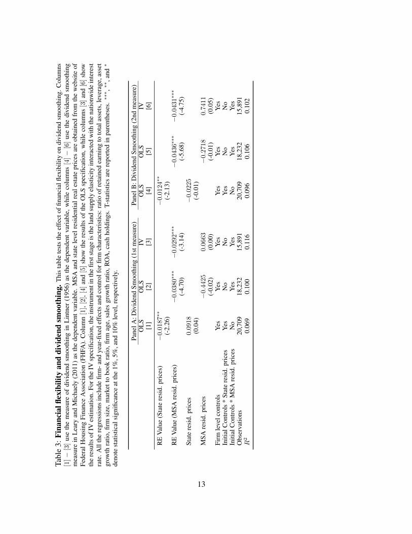
Tabl

e3:

Fina

ncia

lflex

ibili

tyan

ddi

vide

ndsm

ooth

ing.

Thi

sta

ble

test

sth

eef

fect

offin

anci

alfle

xibi

lity

ondi

vide

ndsm

ooth

ing.

Col

umns

[1]−

[3]

use

the

mea

sure

ofdi

vide

ndsm

ooth

ing

inL

intn

er(1

956)

asth

ede

pend

ent

vari

able

,w

hile

colu

mns

[4]−

[6]

use

the

divi

dend

smoo

thin

gm

easu

rein

Lea

ryan

dM

icha

ely

(201

1)as

the

depe

nden

tvar

iabl

e.M

SAan

dst

ate

leve

lres

iden

tialr

eale

stat

epr

ices

are

obta

ined

from

the

web

site

ofFe

dera

lHou

sing

Fina

nce

Ass

ocia

tion

(FH

FA).

Col

umn[1],[2],[4]

and[5]

show

the

resu

ltsof

the

OL

Ssp

ecifi

catio

n,w

hile

colu

mns

[3]

and[6]

show

the

resu

ltsof

IVes

timat

ion.

Fort

heIV

spec

ifica

tion,

the

inst

rum

enti

nth

efir

stst

age

isth

ela

ndsu

pply

elas

ticity

inte

ract

edw

ithth

ena

tionw

ide

inte

rest

rate

.All

the

regr

essi

ons

incl

ude

firm

-and

year

-fixe

def

fect

san

dco

ntro

lfor

firm

char

acte

rist

ics:

ratio

ofre

tain

edea

rnin

gto

tota

lass

ets,

leve

rage

,ass

etgr

owth

ratio

,firm

size

,mar

kett

obo

okra

tio,fi

rmag

e,sa

les

grow

thra

tio,R

OA

,cas

hho

ldin

gs.

T-st

atis

tics

are

repo

rted

inpa

rent

hese

s.∗∗

∗ ,∗∗

,and

∗

deno

test

atis

tical

sign

ifica

nce

atth

e1%

,5%

,and

10%

leve

l,re

spec

tivel

y.

Pane

lA:D

ivid

end

Smoo

thin

g(1

stm

easu

re)

Pane

lB:D

ivid

end

Smoo

thin

g(2

ndm

easu

re)

OL

SO

LS

IVO

LS

OL

SIV

[1]

[2]

[3]

[4]

[5]

[6]

RE

Val

ue(S

tate

resi

d.pr

ices

)−0.0187∗

∗−0.0124∗

∗

(-2.

26)

(-2.

13)

RE

Val

ue(M

SAre

sid.

pric

es)

−0.0380∗

∗∗−0.0292∗

∗∗−0.0436∗

∗∗−0.0431∗

∗∗

(-4.

70)

(-3.

14)

(-5.

68)

(-4.

75)

Stat

ere

sid.

pric

es0.0918

−0.0225

(0.0

4)(-

0.01

)M

SAre

sid.

pric

es−0.4425

0.0663

−0.2718

0.7411

(-0.

02)

(0.0

0)(-

0.01

)(0

.05)

Firm

leve

lcon

trol

sY

esY

esY

esY

esY

esY

esIn

itial

Con

trol

s*

Stat

ere

sid.

pric

esY

esN

oN

oY

esN

oN

oIn

itial

Con

trol

s*

MSA

resi

d.pr

ices

No

Yes

Yes

No

Yes

Yes

Obs

erva

tions

20,7

0918

,232

15,8

9120

,709

18,2

3215

,891

R2

0.06

90.

100

0.11

60.

096

0.10

60.

102

13

Table 4: Real estate owners and payout. This table tests the robustness of the effect of financial flexibilityon the payout policy for firms that are real estate owners. The dependent variable in panel A of this table is cashdividend over lagged PPE and in panel B is share repurchase over lagged PPE. RE OWNER is a dummy that takesthe value of one if the firm owns real estate and zero otherwise. The regressions used in panel A and panel B aresame as the ones presented in columns [4] − [5] of table 2 (for panel A) and of table 3 (for panel B) in the paper.MSA level residential real estate prices are obtained from the website of Federal Housing Finance Association(FHFA). All regressions use MSA-level residential prices, year and firm fixed effect, control for ratio of retainedearning to total assets, leverage, asset growth ratio, firm size, market to book ratio, firm age, sales growth ratio,ROA, cash holdings, real estate ownership and initial controls interacted with MSA-level residential prices. T-statistics are reported in parentheses. ∗∗∗, ∗∗, and ∗ denote statistical significance at the 1%, 5%, and 10% level,respectively.

Panel A: Dividend Paid Panel B: Shares RepurchasedOLS IV OLS IV[1] [2] [3] [4]

RE OWNER * RE Value (MSA resid. prices) 0.0037∗∗∗ 0.0047∗∗∗ 0.0032∗∗∗ 0.0040∗∗∗

(9.14) (10.24) (4.39) (4.83)MSA resid. prices 0.0172 0.0390 −0.2676 −0.3676

(0.05) (0.07) (-0.41) (-0.41)Firm level controls (incl. RE OWNER) Yes Yes Yes YesInitial Controls * MSA resid. prices Yes Yes Yes YesYear FE Yes Yes Yes YesFirm FE Yes Yes Yes YesObservations 18,336 15,986 17,242 15,042R2 0.788 0.781 0.449 0.455

14

Tabl

e5:

Fina

ncia

lflex

ibili

tyan

dpa

yout

:R

obus

tnes

ste

st5a

.Thi

sta

ble

test

sth

ero

butn

ess

ofth

eef

fect

offin

anci

alfle

xibi

lity

onth

epa

yout

polic

yof

the

firm

whi

leco

ntro

lling

for

the

inve

stm

ent.

The

depe

nden

tvar

iabl

ein

colu

mns

[1]−

[3]

isca

shdi

vide

ndov

erla

gged

PPE

and

inco

lum

ns[4]−

[6]

issh

are

repu

rcha

sed

over

lagg

edPP

E.T

here

gres

sion

sus

edin

colu

mns

[1]−

[3]

are

sam

eas

the

ones

pres

ente

din

colu

mns

[3],

[4],

and

[5]o

ftab

le2

inth

epa

perw

ithan

addi

tiona

lcon

trol

ofin

vest

men

t.Si

mila

rly,

regr

essi

ons

used

inco

lum

ns[4]−

[6]

are

sam

eas

the

ones

pres

ente

din

colu

mns

[3],

[4],

and

[5]

ofta

ble

3in

the

pape

rw

ithan

addi

tiona

lco

ntol

ofin

vest

men

t.In

vest

men

tva

riab

leis

defin

edas

capi

tal

expe

nditu

reno

rmal

ized

byla

gged

PPE

.All

the

regr

essi

ons

uses

year

-an

dfir

m-

fixed

effe

cts,

cont

rolf

orra

tioof

reta

ined

earn

ing

toto

tala

sset

s,le

vera

ge,a

sset

grow

thra

tio,fi

rmsi

ze,m

arke

tto

book

ratio

,firm

age,

sale

sgr

owth

ratio

,RO

A,c

ash

hold

ings

,and

initi

alfir

mle

velc

hara

cter

istic

sin

tera

cted

with

real

esta

tepr

ices

.T-s

tatis

tics

are

repo

rted

inpa

rent

hese

s.∗∗

∗ ,∗∗

,and

∗de

note

stat

istic

alsi

gnifi

canc

eat

the

1%,5

%,a

nd10

%le

vel,

resp

ectiv

ely.

Div

iden

d/la

gged

PPE

Shar

eR

epur

chas

e/la

gged

PPE

OL

SO

LS

IVO

LS

OL

SIV

[1]

[2]

[3]

[4]

[5]

[6]

RE

Val

ue(S

tate

resi

d.pr

ices

)0.0030∗

∗∗0.0026∗∗

∗

(9.3

5)(4

.65)

RE

Val

ue(M

SAre

sid.

pric

es)

0.0034∗

∗∗0.0044∗∗

∗0.0030∗

∗∗0.0039∗

∗∗

(8.3

4)(9

.40)

(4.1

1)(4

.75)

Stat

ere

sid.

Pric

es0.3445∗

∗∗0.1187

(7.5

9)(1

.41)

MSA

resi

d.Pr

ices

0.0103

0.0272

−0.2607

−0.3606

(0.0

3)(0

.05)

(-0.

40)

(-0.

40)

Inve

stm

ent

0.0011

0.0008

0.0006

0.0040∗∗

∗0.0036∗

∗∗0.0032∗

∗

(1.5

9)(0

.14)

(0.8

0)(3

.35)

(2.8

1)(2

.36)

Firm

leve

lcon

trol

sY

esY

esY

esY

esY

esY

esIn

itial

Con

trol

s*

Stat

ere

sid.

Pric

esY

esN

oN

oY

esN

oN

oIn

itial

Con

trol

s*

MSA

resi

d.Pr

ices

No

Yes

Yes

No

Yes

Yes

Yea

rFE

Yes

Yes

Yes

Yes

Yes

Yes

Firm

FEY

esY

esY

esY

esY

esY

esO

bser

vatio

ns20

,631

18,1

9415

,857

19,4

6017

,106

14,9

19R

20.

781

0.78

30.

779

0.44

50.

450

0.45

6

15

Tabl

e6:

Fina

ncia

lflex

ibili

tyan

ddi

vide

ndsm

ooth

ing:

Rob

ustn

ess

test

5b.

Thi

sta

ble

test

sth

eef

fect

offin

anci

alfle

xibi

lity

onth

edi

vide

ndsm

ooth

ing

whi

leco

ntro

lling

for

the

inve

stm

ent.

The

base

line

regr

essi

onis

the

spec

ifica

tion

inco

lum

n[1

],[2

],an

d[3

]of

tabl

e3.

Col

umns

[1]−

[3]

use

trad

ition

ally

used

mea

sure

ofdi

vide

ndsm

ooth

ing

asde

pend

ent

vari

able

,whi

leco

lum

ns[4]−

[6]

use

divi

dend

smoo

thin

gm

easu

reas

used

inL

eary

and

Mic

hael

y(2

011)

asth

ede

pend

entv

aria

ble.

The

regr

essi

ons

used

are

sam

eas

the

ones

pres

ente

dta

ble

3w

ithan

addi

tiona

lcon

trol

ofin

vest

men

t.In

vest

men

tvar

iabl

eis

defin

edas

capi

tale

xpen

ditu

reno

rmal

ized

byla

gged

PPE

.All

the

regr

essi

ons

uses

year

-an

dfir

m-

fixed

effe

cts,

cont

rolf

orra

tioof

reta

ined

earn

ing

toto

tala

sset

s,le

vera

ge,a

sset

grow

thra

tio,fi

rmsi

ze,m

arke

tto

book

ratio

,firm

age,

sale

sgr

owth

ratio

,RO

A,c

ash

hold

ings

,and

initi

alfir

mle

velc

hara

cter

istic

sin

tera

cted

with

real

esta

tepr

ices

.T-s

tatis

tics

are

repo

rted

inpa

rent

hese

s.∗∗

∗ ,∗∗

,and

∗de

note

stat

istic

alsi

gnifi

canc

eat

the

1%,5

%,a

nd10

%le

vel,

resp

ectiv

ely. D

ivid

end

Smoo

thin

g(1

stm

easu

re)

Div

iden

dSm

ooth

ing

(2nd

mea

sure

)O

LS

OL

SIV

OL

SO

LS

IV[1

][2

][3

][4

][5

][6

]

RE

Val

ue(S

tate

resi

d.pr

ices

)−0.0181∗∗

−0.0125∗∗

(-2.

17)

(-2.

11)

RE

Val

ue(M

SAre

sid.

pric

es)

−0.0374∗∗

∗−0.0283∗∗

∗−0.0440∗∗

∗−0.0437∗

∗∗

(-4.

60)

(-3.

02)

(-5.

68)

(-4.

78)

Stat

ere

sid.

pric

es0.0670

−0.0513

(0.0

3)(-

0.03

)M

SAre

sid.

pric

es−0.3876

−0.1153

−0.2012

0.5103

(-0.

02)

(-0.

01)

(-0.

01)

(0.0

3)In

vest

men

t0.0431

0.0245

0.0309

0.0332

0.0367

0.0429

(1.2

8)(0

.89)

(1.0

2)(1

.40)

(1.3

9)(1

.45)

Firm

leve

lcon

trol

sY

esY

esY

esY

esY

esY

esIn

itial

Con

trol

s*

Stat

ere

sid.

pric

esY

esN

oN

oY

esN

oN

oIn

itial

Con

trol

s*

MSA

resi

d.pr

ices

No

Yes

Yes

No

Yes

Yes

Yea

rFE

Yes

Yes

Yes

Yes

Yes

Yes

Firm

FEY

esY

esY

esY

esY

esY

esO

bser

vatio

ns20

,532

18,0

9015

,762

20,5

3218

,090

15,7

62R

20.

069

0.10

10.

116

0.09

70.

107

0.10

3

16

Figure 1: Trends in firms segregated by change in the market value of their CRE assets.Panel A shows the average Tobin’s Q for firms which experienced the highest positive change in the value of theircollateralizable real estate assets (top half) as compared to firms which experienced the lowest or negative changein the value of their collateralizable real estate assets (bottom half). Equivalently, panels B, C, and D exhibit thetime series in average debt, average dividend paid, and average shares repurchased by these two groups of firms.

17