The Effect of Energy Efficiency Labeling:

Bunching and Prices in the Irish Residential

Property Market

Marie Hyland, Anna Alberini & Seán Lyons

TEP Working Paper No. 0516

Updated August 2016

Trinity Economics Papers Department of Economics Trinity College Dublin

1

The Effect of Energy Efficiency Labeling: Bunching and Prices in the Irish

Residential Property Market ‡

Marie Hyland,1 Anna Alberini

2 and Seán Lyons

3

This version: August 2016, comments welcome

Abstract.

This paper analyses the system of energy performance certificates in place in Ireland. We

find that having a system with discrete energy-efficiency thresholds causes “bunching”

among properties just on the more favorable side of the label cut-off points. This indicates

that, in the region around the label thresholds, assessors tend to be extra lenient when

evaluating the energy performance of dwellings. We examine possible reasons for this

finding, including the market returns to energy efficiency using home sales data from the

Irish property price register, and conclude that most likely assessors are trying to ingratiate

homeowners to get repeat business. We find evidence of a partial “disconnect” between

sellers’ expectations and buyers’ valuation of properties labeled as more efficient.

Keywords: Residential energy efficiency; Energy Performance Certificates; Bunching

QEL Classification: Q40; Q48; R21.

‡ This research makes use of data compiled by the Central Statistics Office (CSO). The use of data compiled by

the CSO does not imply the endorsement of the CSO in relation to the interpretation or analysis of the data. We

are grateful to Gregg Patrick of the CSO for support with the data. We also wish to gratefully acknowledge

Trutz Haase for facilitating the use of the HP Deprivation Index (Haase and Pratschke, 2012). 1 Economic and Social Research Institute (ESRI) and Trinity College Dublin. Corresponding author. Email:

hylandm1@tcd.ie 2 Department of Agricultural and Resource Economics, University of Maryland.

3 Economic and Social Research Institute (ESRI) and Trinity College Dublin.

2

1. Introduction

Buildings are responsible for 40% of energy use and 36% of CO2 emissions in

Europe. They offer significant opportunities for efficiency improvements and are specifically

targeted in the EU’s Energy Efficiency Directive (European Union, 2012). More stringent

building standards, energy certification schemes and incentives to energy efficiency upgrades

are the principal policy tools to improve the energy performance of the building stock. In this

paper, we examine one of these tools - energy certification.

Energy certificates were introduced to tackle an information asymmetry problem in

housing markets. Before their introduction, prospective buyers or tenants were unable to

observe the energy performance of properties. The energy certificates convey information to

potential buyers or tenants about a property’s energy performance, thus allowing them to take

this into consideration in their decision to buy or rent a property. Energy certification is a

market-based environmental policy tool which should cause positive shifts in the demand for

energy efficient properties, thereby increasing the price and, ultimately, the supply of energy-

efficient dwellings.

In the EU, two designs for energy certificates have been adopted - one based on a

stepped certification scale (see Figure 1) and the other based on a continuous color-band strip

(see Figure A1 in Appendix A). Stepped labels, where a building receives an energy-

efficiency grade (generally a letter grade) based on an underlying continuous measure of

energy performance (see Figure 1 in Section 2), are more commonly used. The use of letter

grades based on an underlying continuous measure means that, at the threshold between one

letter grade and the next, a marginal change in the continuous measure of energy efficiency

causes a discrete change in the rating achieved. If energy efficiency is valued by the market

there is an incentive, from the point of view of home sellers, to fall on the more favorable

side of a threshold. Bunching occurs when there is an excess frequency of homes on the

3

favorable side of a threshold accompanied by a much reduced frequency on the unfavorable

side of that threshold.

Bunching has been well documented in the public finance literature. For example,

Saez (2010), Chetty et al. (2011) and Kleven and Waseem (2013) have found that cutoff

points that result in kinks and notches in income tax regimes can lead to a “bunching” of tax-

filers on the policy-favored side of the threshold. This phenomenon has also been

documented in other domains, including car manufacturing in response to the gas guzzler tax

or the presentation of a new car’s fuel economy (Sallee and Slemrod (2012)) and household

appliances at the standards for the Energy Star certification (Houde (2013)). To the best of

our knowledge, the first authors to provide evidence on the occurrence of bunching in a

building certification scheme were Atasoy and Traxler (2015).

In this paper we ask two research questions regarding the energy efficiency labeling

scheme for homes. First, does a design of the labeling scheme based on letter grades and on

sharp thresholds for assigning such letter grades affect the distribution of certified energy

efficiency? And, second, if so, is the price premium for more efficient properties an

explanation for this effect?

We analyze the potential for bunching in the residential property market. Using data

on housing transactions in Ireland, we ask whether the stepped certification scale leads to

bunching on the more favorable side of the letter-grade thresholds. Somewhat surprisingly,

while in previous analyses of bunching in energy certification schemes (i.e., those for cars

and appliances) the bunching was as a result of “tweaking” in manufacturing processes, we

find the strongest evidence of bunching amongst existing homes rather than newly-built

properties. Bunching thus occurs without any changes being made to the energy performance

of the properties, suggesting that it is due to the behavior of energy efficiency assessors.

4

Using methodologies from the public finance literature we quantify the magnitude of

the bunching response by examining what the distribution of energy efficiency ratings in

Ireland would be under a labeling system that does not use discrete classification thresholds.

Our dataset contains information on each property’s transaction price, which allows us to

estimate the market returns to residential energy efficiency, and to see if they are a potential

reason for bunching.

While our analysis focuses on the Irish context, the implications of our

research extend to other countries. The Irish system of EPCs is part of an EU-wide system

and thus our findings are of relevance to policy makers in all European countries, and indeed

any country that already has, or is considering the implementation of, an energy certification

scheme.

The remainder of the paper is organized as follows. Section 2 gives on overview of

the system of EPCs in place in Ireland. Section 3 discusses earlier literature. Section 4

presents the data used in the analysis, while Section 5 outlines the methodology we use to

quantify bunching. The results of the bunching analysis are presented in Section 6, and

Section 7 discusses possible explanations for why the bunching is occurring. Section 8

concludes.

2. Background

To reduce emissions from the building stock for both new and existing properties, the

European Commission introduced the Energy Performance of Buildings Directive (EPBD,

European Union (2003)). The EPBD introduced binding legislation on the minimum energy

performance of all newly-constructed properties and on existing properties undergoing major

renovation, and required any newly-built property, or any property offered for sale or to let,

to have an Energy Performance Certificate (EPC).

5

The EPBD was transposed into Irish law in 2006. EPCs for residential properties in

Ireland are referred to as Building Energy Ratings (BERs). The Sustainable Energy Authority

of Ireland (SEAI) is responsible for the BER scheme. The EPBD legislation states that, as of

2007, any new property for which planning permission is sought must have a BER certificate.

Furthermore, any existing property offered for sale or to let from January 2009 onwards is

required to have a BER certificate, which must be made available to the buyer or letter at the

point of transaction. The legislation was strengthened in 2010 with the introduction of the

Recast EPBD (European Union, 2010). The Recast legislation requires that, as of January

2013, the BER be stated in all advertisements related to properties offered for sale or to let.

BER labels are assigned based on the energy performance score that a property

receives. This score, expressed in kWh/m2/year, is assigned based on the calculated energy

usage for space and water heating, ventilation and lighting purposes. It is based on assumed

typical occupant behavior (what the SEAI refer to as “standardised operating conditions”),

and does not include energy used for the operation of electrical appliances or equipment

(TVs, fridges, etc.; see Appendix A). Homes are assessed and energy ratings assigned by

licensed, independent BER assessors, and the process is overseen by the SEAI.

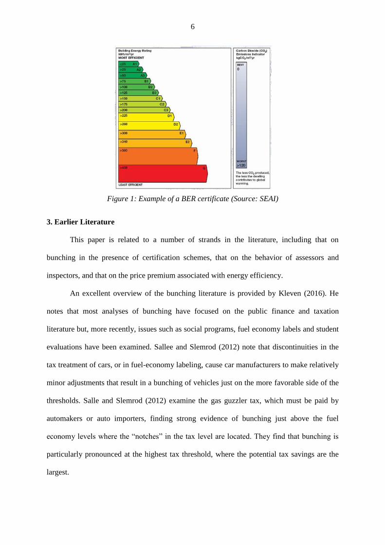
BER certificates are based on a 15-point scale from A1 to G, according on a

property’s energy performance score (its calculated energy usage), where a lower energy use

score results in a better efficiency rating. An example of a BER certificate, which indicates

the energy rating cut-off points, is displayed in Figure 1.

6

Figure 1: Example of a BER certificate (Source: SEAI)

3. Earlier Literature

This paper is related to a number of strands in the literature, including that on

bunching in the presence of certification schemes, that on the behavior of assessors and

inspectors, and that on the price premium associated with energy efficiency.

An excellent overview of the bunching literature is provided by Kleven (2016). He

notes that most analyses of bunching have focused on the public finance and taxation

literature but, more recently, issues such as social programs, fuel economy labels and student

evaluations have been examined. Sallee and Slemrod (2012) note that discontinuities in the

tax treatment of cars, or in fuel-economy labeling, cause car manufacturers to make relatively

minor adjustments that result in a bunching of vehicles just on the more favorable side of the

thresholds. Salle and Slemrod (2012) examine the gas guzzler tax, which must be paid by

automakers or auto importers, finding strong evidence of bunching just above the fuel

economy levels where the “notches” in the tax level are located. They find that bunching is

particularly pronounced at the highest tax threshold, where the potential tax savings are the

largest.

7

Sallee and Slemrod (2012) also find that bunching occurs with the fuel economy

label, where there are no obvious tax savings to be made, but manufacturers exploit the fact

that the labels present the fuel economy as an integer. This suggests that car manufacturers

believe that consumers value fuel economy.

Ito and Sallee (2014) study bunching behavior in the Japanese automobile market. In

Japan, the fuel economy standards for cars are determined by a vehicle’s fuel economy but

are also a step-function of vehicle weight, whereby heavier vehicles are allowed to meet a

lower standard. Ito and Sallee (2014) find that this “double-notched” policy causes vehicle

manufacturers to bunch at vehicle-weight threshold points, where the required levels of fuel-

economy fall. This bunching response results in weight increases for 10% of the vehicles and

exacerbates a number of externalities.

Houde (2014) analyses how appliance manufacturers respond to energy-efficiency

labeling schemes. Houde (2014) examines the “Energy Star” certification in the US, finding

that manufacturers produce goods that just about make the requirement for certification, and

then charge a price premium for these goods. Alberini et al. (2015) use a regression

discontinuity design and matching methods, and document that Swiss auto importers seek to

charge 5-11% more for otherwise similar vehicles that barely attain the “A” fuel economy

label.

Recently, Atasoy and Traxler (2015) use methodologies from the public finance

literature to study bunching in green building certification systems. They uncover evidence of

a supply-side response to energy-efficiency labels in both the US and the UK by measuring

the level of bunching in the Leadership in Energy and Environmental Design (LEED) system

used in the US and in the Building Research Establishment Environmental Assessment

Method (BREEAM) system used in the UK. Using data from the LEED certification scheme,

they also explore the relationship between bunching and corruption indicators and energy

8

prices. They find no relationship between bunching and corruption, but some tentative

evidence that bunching is less prominent in states with lower energy prices.

While some of the papers discussed above document how certifications or standards

based on discrete cutoffs may incentivize manufactures to alter their behavior, in our analysis

we find that bunching is most pronounced in the certification of existing properties. The key

parties in the home energy label process are, of course, the assessors, and so we turn to the

literature to find studies that have examined the incentives and behaviors of testers,

inspectors, and assessors.

An interesting context is the vehicle emissions testing program, which in the US is

often done at decentralized facilities, such as private garages or gas stations. Hubbard (1998,

2002) documents how mechanics falsely pass vehicles undergoing emissions testing in

California. Hubbard (1998) analyses the firm-level characteristics that make some firms more

likely than others to pass a given vehicle. He finds higher rates of lenience at privately-owned

garages (as opposed to state-run test centers) and garages with an increased number of

geographically-close competitors. He hypothesizes that certain firms are more lenient in order

to gain a reputation for “friendliness” and ensure repeat business.

While Hubbard (1998) looks at the behavior of garages conducting smog tests,

Hubbard (2002) examines the behavior of customers who are having their vehicles tested. He

finds that customers are 30% more likely to return to a garage where they have previously

passed a smog check. He also finds that when customers are choosing a garage, they are

sensitive to the garage’s overall pass rate; confirming his previous findings on the importance

of having a “friendly” reputation.

More recent research on the behavior of mechanics conducting emissions testing has

been conducted by Gino and Pierce (2010) and Pierce and Snyder (2012). Gino and Pierce

(2010) find evidence of wealth-based discrimination in vehicle emissions testing, whereby

9

mechanics are more likely to pass consumers in standard, as opposed to high-end, luxury,

vehicles. They also conduct a number of economic experiments with human subjects and find

that this discriminatory behavior is likely driven by envy of wealthier consumers and one’s

empathy towards those of similar wealth levels.

Pierce and Snyder (2012) provide further evidence that overly-lenient mechanics

fraudulently help customers to pass emissions tests. They find strong discontinuities in the

distribution of emission test scores just at the regulatory thresholds. Following a tightening of

emissions standards, 50% of vehicles that would have passed based on the old standards but

should fail based on the new ones have had their test scores shifted into the passing range.

Their analysis suggests that this is the result of illegal behavior by inspectors and not the

result of preemptive repairs being carried out on vehicles.

In the case of fuel economy standards, appliance labels and emissions testing there are

clear monetary incentives to reach a given thresholds (in the case of fuel-economy a lower

tax rate, in the case of appliances a higher price tag, and revenue from the repairs in the case

of smog testing), which raises an obvious question: Are there financial incentives in place

that lead to bunching in energy performance certificates for properties? If the property market

values energy efficiency, and the BER label conveys energy efficiency to potential buyers,

sellers will be able to charge a price premium for properties that achieve a higher efficiency

rating. In this paper, we examine whether this is a possible reason for bunching, using data

from the residential property market in Ireland.

There is ample evidence to suggest that energy efficiency is valued in residential

property markets.4 Early evidence dates back to Gilmer (1989) and Dinan and Miranowski

(1989). More recently, Brounen and Kok (2011) find that in the Netherlands homes that

receive a “green” label are sold at a 3.8% price premium. Cajias and Piazolo (2013) find that

4 A related strand of literature also documents a price premium for energy efficiency in the commercial segment

of the market; see for example Eichholtz et al. (2010, 2013) and Fuerst and McAllister (2011a,b).

10

green certification positively impacts rental rates and market values in Germany, and Fuerst

et al. (2015) show that, in the UK, properties that receive an A or B rating receive a 5%

premium relative to otherwise comparable D-rated properties.

4. The Data

Our dataset was compiled by the Irish Central Statistics Office (CSO) by merging

data from the Irish Property Price Register maintained by the Revenue Commissioners,

SEAI’s register of all issued BER certificates and the All-Island HP Deprivation Index

(Haase and Pratschke, 2012), which provides an indication of the general affluence, and thus

the desirability, of a particular property’s location based on Census data for “small areas.”5

A property price register was established in Ireland in 2010; the data we use from the

Revenue Commissioners contain information on the date of sale, the address and the price of

all properties sold in Ireland from January 2010 until mid-April 2015. This was a difficult

period for the Irish housing market, characterized by low sales volumes, particularly in the

earlier years of our data. The property sales per year are summarized in Table 1 below.

Table 1: Number of property sales per year

Year Number of transactions

2010 13,280

2011 12,646

2012 18,714

2013 22,861

2014 31,606

2015 (to mid-April) 4,359

Total 103,466

5 This is the smallest unit of geographical disaggregation used by the CSO that maintains data confidentiality;

small areas contain between 50 and 200 dwellings.

11

Property transaction data from the Revenue Commissioners were matched with data

from SEAI’s BER register, which includes details of all residential BERs published to date.

The data from SEAI and from the Revenue Commissioners are matched based on each

property’s address. An exact match was not possible for all properties6 and thus our data set

contains information on transaction prices and BER assessments for 77,444 properties –

approximately 75% of all property sales in Ireland over this period. This final dataset covers

virtually all of the sales in urban and suburban areas.

Table 2 presents descriptive statistics for the matched properties in our data. The

average property in our data was sold for €222,834 (in real 2011 values, including VAT), has

an average floor area of 113m2 and has an average calculated energy usage of

292kWh/m2/year. Table 2 also shows that the most common aggregated BER label is a C

rating, and that A-rated properties are very rare. Most of the properties sold during this time

period were existing, rather than newly built, properties (92%), with detached or semi-

detached homes accounting for almost two thirds of the sales (27% and 35%, respectively).

The properties sold are quite diverse in terms of vintage, but the sales generally mirror the

construction boom in Ireland in the 2000s. Twenty-eight percent of the properties sold were

built between 2002 and 2007. The majority of sales were to owner occupiers, with just under

23% of properties being sold to investors.

Table 2: Descriptive statistics

Continuous variables:

Avg. sales price (incl. VAT)

€222,834

Avg. floor area:

113m2

Avg. energy score 292 kWh/m2/yr

Categorical variables:

BER category:

Construction period

A 0.5% Before 1919 7.3%

B 8.9% 1919-1940 6.8%

C 32.3% 1941-1960 9.9%

D 26.1% 1961-1970 5.6%

6 Most unmatched properties are located in rural areas where non-unique addresses meant that an exact match

could not be made.

12

E 14.5% 1971-1980 9.4%

FG 17.8% 1981-1990 9.1%

Main heating fuel: 1991-1995 6.3%

Electricity 12.3% 1996-2001 13.6%

Natural gas 48.3% 2002-2007 28.4%

LPG 1.5% 2008 on 3.7%

Oil-fired 34.8% Coastal dummy:

Renewable 0.2% Non-coastal 92.1%

Solid fuel 2.9% Coastal 7.9%

Property type: New/Second hand:

Ground-floor apt. 4.3% Second-hand 92.2%

Mid-floor apt. 4.7% New 7.8%

Top-floor apt. 3.7% Area type:

Basement 0.0% Mixed 6.3%

Maisonette 0.8% Rural 22.6%

Detached house 26.5% Urban 71.1%

Semi-detached 35.0% Buyer type:

End-of-terrace 7.7% Non Owner-Occupier 22.9%

Mid-terrace 17.3% First-time buyer (FTB) 31.1%

Owner-Occupier, non FTB 46.0%

The BER categories listed in Table 2 are assigned according to the energy use score

each property receives in its energy efficiency evaluation, which is carried out by

independent BER assessors. The energy efficiency scores are calculated using a dedicated

software package, the Dwellings Energy Assessment Procedure (DEAP).7

Preliminary evidence that bunching may be occurring can be inferred from the raw

data. Figure 2 plots the distribution of the calculated energy use score across all properties.

There is clear evidence of bunching just at the more favorable side of the label thresholds

(indicated by dashed vertical lines). Bunching appears to be particularly pronounced at

225kWh/m2/yr; this is the threshold between receiving a C3 versus a D1 energy rating.

7Further details of the DEAP software and assessment procedure are provided in Appendix A.

13

Figure 2: Preliminary evidence of bunching at the label thresholds

5. Methodology: Quantifying Bunching

In order to quantify the extent to which the distribution of energy efficiency is being

affected by having a scheme in place with discrete thresholds, we examine what the

distribution would look like in the absence of these label cut-off points. In order to generate a

counterfactual distribution, we follow a methodology used in the public finance literature to

quantify the behavioral responses to notches and kink points in tax regimes (see for example

Saez (2010); Chetty et al. (2011); Kleven and Waseem (2013)). Following Kleven and

Waseem (2013) who analyze each income tax bracket in isolation, we analyze each BER-

label threshold separately. In doing so we are assuming that if and when an assessor passes a

property from one BER category into a more favorable category by adjusting the continuous

energy rating, he or she moves the property up by only a single grade. We believe that this is

a reasonable assumption.8

8 As noted by Ito and Sallee (2014), this assumption is likely to result in a conservative estimate of bunching, as

we will not account for the bunching response of any properties that “jump” more than one label.

0

.00

2.0

04

.00

6

Den

sity

0 200 400 600Continuous efficiency measure (kWh/m2/yr)

14

We begin by collapsing the properties into integer point bins ( ) based on their

continuous measure of energy use (such that each interval represents 1 kWh/m2/year). We

then count the number of properties in each bin. In order to estimate the counterfactual

distribution, we fit a flexible polynomial to the empirical energy-use distribution, omitting the

contribution of a range of observations surrounding each threshold where we assume

bunching is occurring. The regression takes the form:

where is the number of properties in bin , is the level of energy efficiency in bin , and

is the order of the polynomial. and refer to the upper and lower bound of the excluded

range – this is the area of the distribution that we believe is being affected by bunching. We

estimate the counterfactual distribution excluding the observations in the excluded range, and

predict the counterfactual number properties per bin:

. The excess

bunching on the favourable side of each BER threshold is defined as the difference between

the true and the counterfactual number of observations in the bins from the lower bound of

the excluded range up to the threshold point ( ):

. The excess

observations on the favourable side of the cutoff are “missing” observations from the

unfavorable side, thus the missing mass is defined as: .

Bunching is sharp in the area below the cutoff and so, following Kleven and Waseem

(2013), the lower bound of the excluded range ( ) can be determined visually. As the area of

missing mass above the threshold is more diffuse, the upper bound ( ) is determined such

that the total number of excess observations on the favorable side of the threshold

approximately equals the total number of missing observations on the unfavorable side. In

other words, we determine such that ˆ ˆB M . To ensure the robustness of our estimates we

15

conduct sensitivity analyses as to the degree of the polynomial ( used to estimate , and as

to the lower bound of the excluded range where bunching begins ( ).

We calculate two estimates of bunching: i) the total number of extra observations in

the excluded range on the favorable side of the threshold ( ), and ii) a relative measure of

bunching ( ) which is the total excess mass relative to the average number of observations in

the excluded range as per the counterfactual distribution (i.e., the average from to ).

Following Chetty et al. (2011), we calculate the standard errors on the bunching estimates

using a parametric bootstrapping procedure, whereby we draw from the estimated vector of

errors ( ) to generate a new set of property counts and follow the steps explained above to

estimate absolute bunching ( ) and relative bunching ( ). The standard errors are thus

defined as the standard deviation of the distribution of these estimates.

6. Results

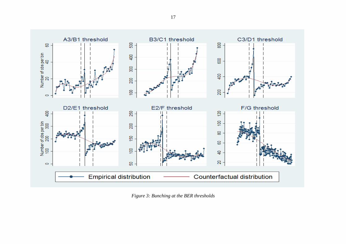
We find strong evidence of bunching across the BER label categories, although the

bunching response is stronger at some label thresholds than others. In particular we note that

bunching is more pronounced at the thresholds where the letter changes (e.g., from B3 to C1)

relative to the thresholds within letter grades (e.g., from B2 to B3) (see Table 3). Figure 3

plots the empirical distribution against the counterfactual distribution (estimated by fitting the

flexible polynomial outlined in the previous section) at each letter grade threshold (i.e., the

cutoff points between A3 and B1, B3 and C1, etc.). In each case there is clear excess

bunching on the favorable side of the threshold, accompanied by missing mass at the

unfavorable side.

The graphs in Figure 3 illustrate the excess bunching. The dashed vertical lines

represent the lower and upper bounds of the excluded range. In all cases we choose a

conservative range of observations to exclude. This will reduce the potential bias in our

16

estimates due to possible misspecification of the polynomial. On the other hand it may result

in an under-estimate of the magnitude of bunching.

It is clear that bunching is less sharp at some thresholds than others. For example,

there is a lot more noise at the cut-off between A3 and B1 labels. As these labels imply very

high levels of energy efficiency, there are very few observations here (only 1.3% of

properties in our sample have a B1 rating or better). It is also possible that, at this level of

energy efficiency, it is harder to make small adjustments to the continuous measure of

efficiency such that a property makes the next grade.

Table 3 shows that the absolute number of excess observations is largest just on the

favorable side of the C3 label threshold. In the narrow region on the more favorable side of

the C3 threshold there 817 extra observations, relative to what the counterfactual distribution

predicts there would be in the absence of the label notch. However, the counterfactual

number of observations per bin is also highest here, so the relative amount of bunching is not

largest. Relative bunching is most pronounced at the cutoff between D and E letter grades,

and at the very end of the BER scale, between F and G labels. At the threshold between D2

and E1 labels, there are 3.3 times as many observations as predicted by the counterfactual

distribution, while between F and G labels relative bunching is 3.1 times the counterfactual

number of observations. This may indicate reluctance among assessors to assign the worst

BER labels to properties. At the opposite end of the scale, we see that the total number of

excess observations at the favorable side of the A3 threshold is low; however, the relative

degree of bunching is large here as there are relatively few properties in this area of the

distribution.

17

Figure 3: Bunching at the BER thresholds

18

Table 3: Total estimated excess mass ( ) and relative magnitude of bunching ( )

Threshold

A3 – B1 33.80 (6.02)*** 2.52 (0.87)***

B1 – B2 17.96 (2.02)*** 0.48 (0.08)***

B2 – B3 88.27 (15.63)*** 0.80 (0.18)***

B3 – C1 326.25 (40.38)*** 1.40 (0.25)***

C1 – C2 320.19 (44.10)*** 1.02 (0.19)***

C2 – C3 372.65 (49.87)*** 1.04 (0.19)***

C3 – D1 816.52 (100.20)*** 2.35 (0.45)***

D1 – D2 278.50 (20.85)*** 1.03 (0.10)***

D2 – E1 616.43 (91.76)*** 3.29 (0.71)***

E1 – E2 108.66 (11.96)*** 0.73 (0.11)***

E2 – F 245.47 (9.43)*** 2.23 (0.15)***

F – G 193.03 (8.50)*** 3.10 (0.18)*** Note: Standard errors, calculated using parametric bootstrapping, in parentheses. *** p < 0.01. Bold font

highlights where the letter grade changes – bunching is always more pronounced at these points.

Table 3 also indicates that bunching is much more pronounced at the thresholds where

the letter grade changes (for example, B3-C1, C3-D1, etc.). Thresholds within letter grades

result in much less bunching, here the values of are often less than one indicating that the

bunching response is small, albeit statistically significant.

7. What are the Reasons for Bunching?

In Section 6 we documented visual and statistical evidence of bunching of properties

at the cutoffs between one energy efficiency category and the next. In this section, we

discuss, and look for evidence to back up or rule out, possible reasons why bunching occurs.

The first possible reason is that bunching is simply an artifact of the algorithm used to

compute the home’s energy consumption rate. However, experts within SEAI (the designated

BER issuing authority) with whom we spoke ruled out this possibility.9

When data for a particular property is missing, many assessment packages (including,

for example, the Standard Assessment Procedure used in the UK; see below) impute the

average values for homes of the same vintage. While in principle this could result in a

“lumpy” distribution of energy efficiency scores, there is no reason why this should result in

9 We are grateful to SEAI staff who answered our queries relating to this matter.

19

bunching at the thresholds. Moreover, data from similar programs and software in other

countries—such as the Standard Assessment Procedure efficiency scores, which were

assigned to the homes covered by the English House Conditions Survey—follow a smooth

distribution and do not exhibit bunching.10

To further verify that the bunching we observe is not an artifact of the DEAP

software, we look for evidence of bunching in a sub-sample of properties where we believe

the incentives to bunch are weakest. Specifically, we use the database of all BER certificates

issued to date11

and look for evidence of bunching for the properties designated as “social

housing lettings,” and compare these to properties offered for private lettings. For social

lettings (housing made available to, for example, low-income families and people with

disabilities) the property owners will not be trying to extract extra rent from lessees for more

energy-efficient properties, and thus we believe that the incentives to bunch are lowest here.

Figure A3 in Appendix C compare the distribution of energy efficiency for properties

designated for social housing rental with those for private letting. As is clear from these

graphs, we do not observe the same bunching pattern for social housing. This provides further

evidence that the bunching we observe in our data is not an artifact of the DEAP software.

We check whether the energy efficiency of a home affects its sale value below, but we

note that assessors charge a flat fee for their services, and their earnings are not directly

linked to the sale price of a home. They therefore do not have a direct incentive to overstate

the energy efficiency of a home. They do not have a direct incentive to understate it either,

10

We obtained the data from the 2009 wave of the English House Conditions Survey. The Standard Assessment

Procedure (SAP) score range from 1 to 84.5, where a higher figure denotes better efficiency. The UK Energy

Performance Certification, which assigns letter grades ranging from A (best) to G (worst), is based on the

interval where the SAP score falls. For example, the current standard for attaining an A grade is a SAP score of

92 or more. We did not observe any discontinuities or spikes in the distribution of the SAP scores. Our findings

are thus in contrast with those reported for the UK in Comerford et al. (2016), who attribute bunching to minor

fixes and repairs done by owners. We judge this explanation based on behaviors as unlikely, since the energy

consumption rate is computed following a government-approved procedure based on structural characteristics of

the home, and the assessment is not conducted in such a way that warns owners about the potential for

improvement (in other words, there is no testing and re-testing). 11

Available for download from the National BER Research Tool:

https://ndber.seai.ie/BERResearchTool/Register/Register.aspx

20

since, unlike vehicle emissions testing programs, there is no obligation to do repairs to a

home that does, or does not, attain a certain BER level.

An earlier study based on homes sales and lettings in Ireland from 2008 to 2012

(Hyland et al., 2013) found that asking prices were strongly influenced by the BER

attainment. Owners of A-rated homes asked for 9% more, all else the same, than a

comparable home with a D rating. We use the final transaction prices documented in our

dataset, along with house characteristics and BER status, to see whether final prices actually

mirror the energy performance of a home.

We use the well-established hedonic price model (Rosen, 1974), and fit the equation:

ln i i i i i i iP X BER Z T (2)

where, ln iP is the log of sales price of property i; iX represents the property-specific

variables associated with property i (other than the energy label); iBER is a dummy variable

indicating which BER label (from A to G) property i receives; and iZ represents a vector of

county and Dublin-postcode dummies12

to control for the large impact that location has on

property prices. iT controls for the year and month in which property i was sold – this

captures changes in the economy-wide selling conditions over time and seasonality; finally,

i represents the error term.

The BER labels are assigned on a 15-point scale from A1 to G (see Figure 1);

however, as there are very few A-rated properties in our sample,13

we collapse the A1, A2

and A3 properties into a single “A” category. The main results from the regressions are

presented in Table 4.

12

A full nationwide system of postcodes was not introduced in Ireland until July 2015. 13

After excluding extreme outliers from the sample, there is only one A1 property in our sample, 25 A2

properties and 321 A3-rated properties

21

Table 4: Effect of BER labels on transaction prices

Y: log (Price ex.VAT) Baseline Dublin only From 2013 on

A (aggregated) 0.229 (0.023)*** 0.114 (0.030)*** 0.248 (0.029)***

B1 0.180 (0.020)*** 0.107 (0.025)*** 0.265 (0.028)***

B2 0.128 (0.013)*** 0.072 (0.015)*** 0.208 (0.019)***

B3 0.123 (0.009)*** 0.049 (0.011)*** 0.184 (0.013)***

C1 0.125 (0.008)*** 0.083 (0.010)*** 0.168 (0.011)***

C2 0.136 (0.008)*** 0.088 (0.009)*** 0.172 (0.011)***

C3 0.151 (0.007)*** 0.099 (0.009)*** 0.178 (0.010)***

D1 0.135 (0.007)*** 0.088 (0.008)*** 0.159 (0.010)***

D2 0.132 (0.007)*** 0.096 (0.008)*** 0.145 (0.009)***

E1 0.119 (0.007)*** 0.076 (0.008)*** 0.130 (0.010)***

E2 0.123 (0.007)*** 0.082 (0.008)*** 0.136 (0.009)***

F 0.081 (0.007)*** 0.058 (0.008)*** 0.081 (0.010)***

G Reference

Observations 74,701 28,927 42,615

R-squared 0.726 0.753 0.747 Notes: Robust standard errors in parentheses. *** p < 0.01, ** p < 0.05, * p < 0.1. For a full list of control

variables please refer to Appendix B.

Table 4 shows that more energy-efficient properties transact at a price premium. For

the baseline sample, A-rated properties transact at a price premium of 26% relative to

otherwise comparable G-rated properties, and B1 properties at a 20% premium. However, in

the baseline sample the returns to energy efficiency are not monotonic. For example, the

returns to C3-rated properties are greater than the return to B3-rated properties. Moreover, at

the higher end of the efficiency scale, the price premiums between adjacent label categories

are often not statistically different, indicating that the property market does not generally

award a price premium for single label-grade increases in energy efficiency.

Table 4 also shows that the returns to energy efficiency are significantly smaller in the

Dublin metro area (where energy efficiency is presumably trumped by other considerations

and demand and supply conditions; see Hyland et al., 2013), and larger for the nation as a

whole from 2013 onwards, when they generally follow a monotonic pattern. As 2013 was the

year when the strengthened “Recast” BER legislation came into effect, these larger and more

consistent returns suggest that the Recast legislation achieved its desired effect of increasing

the awareness of energy efficiency.

22

An interesting result of these regressions is that while they suggest a general positive

effect of efficiency labels on property prices (with the exception of Dublin), the differences

between adjacent label categories are not always statistically significant. This is despite the

fact that we see significant bunching at all letter-grade thresholds.

Taken together, the evidence from Hyland et al. (2013), and the regressions in Table 4

suggest that while sellers appear to have a strong preference for receiving a better efficiency

label, the market does not always reward the higher label, at least not in terms of selling

price. This suggests a disconnect between sellers’ expectations of the returns to energy

efficiency and the market valuation of it.

Based on these findings, we speculate that bunching occurs not because assessors can

realize immediate gains from the price premium associated with the sale of more energy-

efficient properties, but because they hope to ingratiate their customers (the home sellers),

who do believe a better BER rating means a better sale price. This will generate repeat

business for the assessor and word-of-mouth recommendations that generate future business.

It is important to note that the efficiency thresholds have remained unchanged since the

inception of the scheme, and no significant changes have been made to the DEAP software.

The consistency of the thresholds and methodology, we believe, makes “bunching” more

likely as it removes any uncertainty among assessors as to how much the continuous energy

use score needs to be adjusted to move a property to the favorable side of a threshold.

It is possible that bunching is occurring for other reasons as well. Having a better

BER label may be associated with other positive market outcomes; for example, more highly-

rated homes may sell faster. Unfortunately we have no information on how long the

properties in our data were on the market for, and thus leave analysis of this potential channel

to future research.

23

8. Discussion and concluding remarks

In this paper we show that having an energy rating scheme in which properties are

assigned energy labels based on a continuous measure of energy efficiency leads to bunching,

i.e., discontinuities in the distribution, just on the more favorable side of the label thresholds.

In the region of the thresholds, marginal changes in the continuous measure can lead to large

and discrete changes in the outcome achieved.

We find that the bunching is particularly strong at the lower end of the efficiency

scale. This may be reflective of a reluctance to assign the most energy inefficient labels to

properties. Different magnitudes of bunching at different points along the BER scale may

also reflect a constraint on the possibility of “tweaking” the energy-efficiency scores, which

may be easier to do at some thresholds relative to others.14

Our results are robust with respect

to numerous checks (see Appendix C).

As we have data on the sales price of these properties, we investigate whether this

bunching behavior correlates with premiums in sales prices associated with receiving a better

label. Using hedonic regression techniques we find that while energy efficiency is generally

positively valued in the Irish property market, the differences between the premiums received

by adjacent label categories are generally not significant. We do find however that there is a

significant penalty for receiving the worst possible efficiency rating, relative to receiving the

second-worst label. Thus, while we find evidence of significant bunching behavior across the

entire range of labels, we generally only find evidence of a sales price effect at the lower end

of the efficiency scale. This suggests that there is a disconnect between sellers’ expectations

of the returns to energy efficiency and the market’s valuation of it, at the higher end of the

scale.

14

Numerous parameters are inputted by the assessors into the DEAP software - many of which are discrete

rather than continuous in nature, which may constrain the potential pattern of bunching

24

While it is important to consider the behavior of the buyers and sellers in this market,

the behavior of another set of agents, i.e., the independent assessors, should also be

considered. BER assessors are intermediate agents who are relied upon to implement the

energy certification scheme. Our results show that these assessors are facing some incentives

that are leading to perverse behavior (from the point of view of the certification scheme) in

the region of the thresholds. The earnings of BER assessors are not directly linked to the sales

price of a home, and for this reason, there is no direct incentive to overstate energy

efficiency. However, we speculate that assessors may behave in a way that is systematically

different when a property is in the region of a threshold in order to ingratiate property sellers

and generate future business via word-of-mouth recommendations. Research from other

fields has demonstrated that experts sometimes act in ways that are overly-lenient towards

consumers to ensure repeat business and to win customers in competitive markets.

There are a number of policy implications that can be drawn from our analysis. Our

evidence of bunching illustrates a potential downside to having a certification scheme in

place based on discrete notches. The strong evidence we find of bunching across the BER

scale indicates that tighter auditing of the system may be warranted.15

The fact that assessors

are being more generous in their evaluations in the vicinity of the thresholds indicates a

degree of non-compliance which has, heretofore, gone unnoticed. If buyers were to become

aware of this bunching behavior, it may erode trust in the certification scheme making buyers

less willing to pay a premium for energy efficiency. This may in turn act as a barrier to the

provision of a more energy-efficient housing stock. Furthermore, if information asymmetry is

the market failure that energy labels are trying to address, it is crucial that these labels

accurately represent information about the energy efficiency of all properties – including

those whose efficiency levels fall in the vicinity of the thresholds. Finally, it is worth

15

Indeed the SEAI have themselves highlighted (SEAI, 2015) a number of problem areas in the BER assessment

procedure which they will be targeting in future audits. Such enforcement activity may help alleviate the

bunching phenomenon..

25

highlighting that the methodologies we have used to estimate bunching in this paper could be

applied by the regulator to assess where discontinuities in the energy-efficiency distribution

are most pronounced, and thus target their resources at auditing these areas.

References

Alberini, A., Bareit, M. and Filippini, M., 2014. Does the Swiss Car Market Reward Fuel

Efficient Cars? Evidence from Hedonic Pricing Regressions, a Regression Discontinuity

Design, and Matching, Working Paper.

Atasoy, A. T. and Traxler, C., 2015. Economics of Bunching: Evidence from Green Building

Certification Systems. Working Paper.

Brounen, D. and Kok, N., 2011. On the economics of energy labels in the housing market,

Journal of Environmental Economics and Management, 62(2), 166-179.

Cajias, M. and Piazolo, D., 2013. Green performs better: energy efficiency and financial

return on buildings, Journal of Corporate Real Estate, 15(1), 53-72.

Chetty, R., Friedman, J. N., Olsen, T. Pistaferri, L., 2011. Adjustment Costs, Firm Responses,

and Micro vs. Macro Labor Supply Elasticities: Evidence from Danish Tax Records,

Quarterly Journal of Economics, 126, 749-804.

Comerford, D., Lange, I. and Moro, M. 2016. The Supply-side Effects of Energy Efficiency

Labels, Colorado School of Mines working paper 2016-01, Golden, CO, January.

Dinan, T. M. and Miranowski, J. A., 1989. Estimating the implicit price of energy efficiency

improvements in the residential housing market: A hedonic approach, Journal of Urban

Economics, 25(1), 52-67.

Eichholtz, P., Kok, N. and Quigley, J. M., 2010. Doing well by doing good? Green office

buildings. The American Economic Review, 2492-2509.

Eichholtz, P., Kok, N. and Quigley, J. M., 2013. The economics of green building. Review of

Economics and Statistics, 95(1), 50-63.

European Commission, 2011. Energy Efficiency Plan 2011. Communication from the

Commission to the European Parliament, the Council, the European Economic and Social

Committee and the Committee of the Regions.

European Union, 2003. DIRECTIVE 2002/91/EC OF THE EUROPEAN PARLIAMENT

AND OF THE COUNCIL of 16 December 2002 on the energy performance of buildings,

Official Journal of the European Communities, 46.

European Union, 2010. DIRECTIVE 2010/31/EU OF THE EUROPEAN PARLIAMENT

AND OF THE COUNCIL of 19 May 2010 on the energy performance of buildings (recast),

Official Journal of the European Union, 53.

26

European Union, 2012. DIRECTIVE 2012/27/EU OF THE EUROPEAN PARLIAMENT

AND OF THE COUNCIL of 25 October 2012 on energy efficiency, amending Directives

2009/125/EC and 2010/30/EU and repealing Directives 2004/8/EC and 2006/32/EC, Official

Journal of the European Union, 55.

Fuerst, F., McAllister, P., 2011a. Green noise or green value? Measuring the effects of

environmental certification on office values. Real Estate Economics, 39, 45-69.

Fuerst, F., McAllister, P., 2011b. Eco-labeling in commercial office markets: Do LEED and

Energy Star offices obtain multiple premiums? Ecological Economics, 70, 1220-1230.

Fuerst, F., McAllister, P., Nanda, A. and Wyatt, P., 2015. Does energy efficiency matter to

home-buyers? An investigation of EPC ratings and transaction prices in England, Energy

Economics, 48, 145-156.

Gino, F. and Pierce, L., 2010. Robin Hood under the hood: Wealth-based discrimination in

illicit customer help, Organization Science, 21 (6), 1176-1194.

Haase, T. and Pratschke, J., 2012. The 2011 Pobal HP Deprivation Index for Small Areas

(SA) - Introduction and Reference Tables. Technical Report.

Houde, S., 2014. Bunching with the Stars: How firms respond to environmental certification.

Working paper.

Hubbard, T., N., 1998. An Empirical Examination of Moral Hazard in the Vehicle Inspection

Market, The RAND Journal of Economics, 29 (2), 406-426.

Hubbard, T., N., 2002. How do consumers motivate experts? Reputational incentives in an

auto repair market, Journal of Law and Economics, 45 (2), 437-468.

Hyland, M., Lyons, R. C. and Lyons, S., 2013. The value of domestic building energy

efficiency - Evidence from Ireland, Energy Economics, 40, 943-952.

Ito, K. and Sallee, I., 2015. The Economics of Attribute-Based Regulation: Theory and

Evidence from Fuel-Economy Standards. Working Paper.

Kleven, H., 2016. Bunching, Annual Review of Economics, 8.

Kleven, H. and Waseem, M., 2013. Using Notches to Uncover Optimization Frictions and

Structural Elasticities: Theory and Evidence from Pakistan. Quarterly Journal of Economics,

128, 669-723.

Pierce, L. and Snyder, J. A., 2012. Discretion and Manipulation by Experts: Evidence from a

Vehicle Emissions Policy Change, The B.E. Journal of Economic Analysis and Policy, 12 (3).

Saez, E., 2010. Do Taxpayers Bunch at Kink Points? American Economic Journal: Economic

Policy, 2, 180-212.

27

Sallee, J. and Slemrod, J., 2012. Car Notches: Strategic Automaker Responses to Fuel

Economy Policy. Journal of Public Economics, 96, 981–999.

SEAI, 2012. Dwelling Energy Assessment Procedure (DEAP) Version 3.2.1: Irish official

method for calculating and rating the energy performance of dwellings. Available from:

http://www.seai.ie/Your_Building/BER/BER_Assessors/Technical/DEAP/DEAP_2009/DEA

P_Manual.pdf [Accessed: 23rd October 2015]

SEAI, 2014. A Guide to Building Energy Rating for Homeowners. Available from:

http://www.seai.ie/Your_Building/BER/Your_Guide_to_Building_Energy_Rating.pdf

[Accessed: 22nd October 2015]

SEAI, 2015. BER Assessors – Dwellings Technical Bulletin, Issue No. 1/15, December 2015.

Available from: http://www.seai.ie/Your_Building/BER/DBER-Tech-Bulletin-Dec-2015.pdf

[Accessed: 7th January 2016]

SEAI (n.d.). Introduction to DEAP for professionals. Available from:

http://www.seai.ie/Your_Building/BER/BER_Assessors/Technical/DEAP/Introduction_to_D

EAP_for_Professionals.pdf [Accessed Accessed: 22nd October 2015]

Wiley, J. A., Benefield, J. D. and Johnson, K. H., 2010. Green design and the market for

commercial office space, The Journal of Real Estate Finance and Economics, 41(2), 228-

243.

28

Appendix A: Further information on Energy Performance Certificates

Example of a continuous energy performance label:

Figure A1: The EPC design used in the Flanders region of Belgium

BER assessment procedure and DEAP software

As described in SEAI (2014), a BER is assigned according to a dwelling’s calculated energy

usage for space and water heating and lighting purposes, under standard operating conditions.

Factors which determine the calculated energy usage include dimensions, orientation,

insulation, efficiencies of water and space heating systems, and the proportion of energy-

efficient lighting. Independent certified BER assessors inspect the property and input the

energy-related characteristics into a specific software - the Dwellings Energy Assessment

Procedure (DEAP); the official software used in Ireland for calculating the energy

performance of buildings. The software guides the BER assessors through the following tabs:

Start: Property and assessor details

Dimensions

Ventilation

29

Building elements (including information on U-values)

Water heating

Lighting and internal gains

Net space heating demand

Dist. system losses and gains

Energy requirements

Summer internal temperature

Results

The assessors input information on the above features based on their observed assessment. If

information on a particular input is not available, conservative default values are given in the

DEAP manual (SEAI, 2012). There are strict guidelines to which the BER assessors are

expected to adhere to avoid incorrect data entry (SEAI, n.d.).

Since the BER system was introduced the energy grade thresholds have never been

changed, and no significant changes have been made to the DEAP software.16

For further

details of the DEAP software, a guide is available from the SEAI.17

16

As confirmed by email correspondence with the SEAI on January 8th

, 2016. 17

www.seai.ie/Your_Building/BER/BER_Assessors/Technical/DEAP

30

Appendix B: Full hedonic results (including control variables)

Y: Log(Price excl. VAT) Baseline Dublin only From 2013 on

BER label:

(ref: G)

A (aggregate) 0.229 (0.023)*** 0.114 (0.030)*** 0.248 (0.029)***

B1 0.180 (0.020)*** 0.107 (0.025)*** 0.265 (0.028)***

B2 0.128 (0.013)*** 0.072 (0.015)*** 0.208 (0.019)***

B3 0.123 (0.009)*** 0.049 (0.011)*** 0.184 (0.013)***

C1 0.125 (0.008)*** 0.083 (0.010)*** 0.168 (0.011)***

C2 0.136 (0.008)*** 0.088 (0.009)*** 0.172 (0.011)***

C3 0.151 (0.007)*** 0.099 (0.009)*** 0.178 (0.010)***

D1 0.135 (0.007)*** 0.088 (0.008)*** 0.159 (0.010)***

D2 0.132 (0.007)*** 0.096 (0.008)*** 0.145 (0.009)***

E1 0.119 (0.007)*** 0.076 (0.008)*** 0.130 (0.010)***

E2 0.123 (0.007)*** 0.082 (0.008)*** 0.136 (0.009)***

F 0.081 (0.007)*** 0.058 (0.008)*** 0.081 (0.010)***

Property type:

(ref: Semi-detached house)

Ground-floor apartment -0.226 (0.008)*** -0.210 (0.010)*** -0.236 (0.011)***

Mid-floor apartment -0.297 (0.008)*** -0.203 (0.010)*** -0.331 (0.011)***

Top-floor apartment -0.265 (0.008)*** -0.219 (0.010)*** -0.288 (0.010)***

Basement dwelling 0.203 (0.412) 0.046 (0.449) 0.241 (0.472)

Maisonette -0.209 (0.014)*** -0.202 (0.017)*** -0.243 (0.019)***

Detached house 0.110 (0.004)*** 0.110 (0.007)*** 0.119 (0.006)***

End-of-terrace house -0.077 (0.005)*** -0.066 (0.006)*** -0.086 (0.007)***

Mid-terrace house -0.137 (0.004)*** -0.113 (0.005)*** -0.151 (0.005)***

Period of Construction:

(ref: 2002-2007)

Before 1919 0.086 (0.009)*** 0.251 (0.012)*** 0.125 (0.012)***

1919-1940 0.121 (0.008)*** 0.265 (0.010)*** 0.170 (0.011)***

1941-1960 0.153 (0.007)*** 0.256 (0.009)*** 0.213 (0.009)***

1961-1970 0.153 (0.007)*** 0.254 (0.009)*** 0.203 (0.010)***

1971-1980 0.101 (0.006)*** 0.181 (0.008)*** 0.136 (0.008)***

1981-1990 0.096 (0.006)*** 0.179 (0.007)*** 0.121 (0.008)***

1991-1995 0.092 (0.006)*** 0.141 (0.007)*** 0.123 (0.008)***

1996-2001 0.060 (0.004)*** 0.101 (0.007)*** 0.079 (0.006)***

2008 on 0.005 (0.010) -0.001 (0.015) 0.036 (0.014)**

Buyer type:

(ref: Owner-occ., non-FTB)

First-time buyer (FTB), owner-occ. -0.043 (0.003)*** -0.049 (0.003)*** -0.043 (0.004)***

Non-owner occupier -0.150 (0.004)*** -0.131 (0.006)*** -0.158 (0.005)***

County and postcode dummies:

(ref: Cork county)

Carlow County -0.214 (0.014)*** -0.192 (0.018)***

Cavan County -0.454 (0.016)*** -0.491 (0.019)***

Clare County -0.222 (0.011)*** -0.259 (0.015)***

Cork City 0.160 (0.009)*** 0.173 (0.013)***

Donegal County -0.368 (0.013)*** -0.395 (0.016)***

Dun Laoghaire-Rathdown 0.707 (0.007)*** 0.118 (0.008)*** 0.829 (0.009)***

Fingal 0.397 (0.007)*** -0.149 (0.008)*** 0.466 (0.009)***

Galway City 0.175 (0.009)*** 0.220 (0.013)***

Galway County -0.219 (0.013)*** -0.225 (0.016)***

Kerry County -0.143 (0.012)*** -0.169 (0.016)***

Kildare County 0.144 (0.008)*** 0.198 (0.010)***

Kilkenny County -0.118 (0.013)*** -0.099 (0.017)***

Laois County -0.319 (0.013)*** -0.298 (0.016)***

Leitrim County -0.526 (0.020)*** -0.548 (0.024)***

Limerick City -0.097 (0.013)*** -0.155 (0.015)***

Limerick County -0.180 (0.012)*** -0.209 (0.016)***

31

Longford County -0.637 (0.021)*** -0.652 (0.024)***

Louth County -0.090 (0.010)*** -0.082 (0.014)***

Mayo County -0.285 (0.014)*** -0.316 (0.017)***

Meath County 0.055 (0.008)*** 0.088 (0.011)***

Monaghan County -0.282 (0.022)*** -0.325 (0.027)***

North Tipperary -0.257 (0.017)*** -0.251 (0.021)***

Offaly County -0.203 (0.017)*** -0.223 (0.022)***

Roscommon County -0.547 (0.017)*** -0.559 (0.022)***

Sligo County -0.292 (0.014)*** -0.295 (0.018)***

South Dublin 0.446 (0.007)*** -0.117 (0.008)*** 0.541 (0.009)***

South Tipperary -0.267 (0.015)*** -0.294 (0.018)***

Waterford City -0.253 (0.012)*** -0.259 (0.015)***

Waterford County -0.169 (0.015)*** -0.172 (0.019)***

Westmeath County -0.253 (0.011)*** -0.246 (0.015)***

Wexford County -0.157 (0.010)*** -0.148 (0.013)***

Wicklow County 0.345 (0.009)*** 0.392 (0.012)***

Dublin1 0.436 (0.016)*** -0.118 (0.016)*** 0.534 (0.021)***

Dublin10 0.371 (0.021)*** -0.243 (0.021)*** 0.424 (0.032)***

Dublin11 0.408 (0.011)*** -0.201 (0.012)*** 0.464 (0.015)***

Dublin12 0.529 (0.011)*** -0.097 (0.011)*** 0.637 (0.016)***

Dublin13 0.509 (0.013)*** -0.043 (0.013)*** 0.612 (0.019)***

Dublin14 0.796 (0.029)*** 0.187 (0.027)*** 0.947 (0.033)***

Dublin15 0.569 (0.017)*** -0.006 (0.016) 0.726 (0.023)***

Dublin17 0.454 (0.024)*** -0.164 (0.026)*** 0.498 (0.028)***

Dublin2 0.629 (0.017)*** 0.076 (0.017)*** 0.767 (0.023)***

Dublin20 0.414 (0.030)*** -0.166 (0.026)*** 0.451 (0.040)***

Dublin3 0.664 (0.010)*** 0.046 (0.010)*** 0.778 (0.015)***

Dublin4 0.836 (0.013)*** 0.245 (0.012)*** 0.976 (0.016)***

Dublin5 0.605 (0.012)*** 0.000 (0.012) 0.729 (0.015)***

Dublin6 0.850 (0.014)*** 0.255 (0.014)*** 0.986 (0.020)***

Dublin6w 0.636 (0.013)*** 0.017 (0.012) 0.774 (0.018)***

Dublin7 0.559 (0.011)*** -0.055 (0.011)*** 0.658 (0.015)***

Dublin8 0.518 (0.012)*** -0.090 (0.012)*** 0.625 (0.015)***

Dublin9 0.613 (0.009)*** 0.720 (0.013)***

Number of stories -0.044 (0.004)*** -0.044 (0.005)*** -0.047 (0.005)***

Number of chimneys 0.017 (0.002)*** 0.022 (0.002)*** 0.015 (0.003)***

Log (Total floor area) 0.641 (0.007)*** 0.693 (0.010)*** 0.628 (0.009)***

New home dummy -0.089 (0.007)*** -0.103 (0.011)*** -0.152 (0.009)***

Coastal dummy 0.142 (0.007)*** 0.062 (0.011)*** 0.144 (0.009)***

Log (Area population density) 0.015 (0.002)*** -0.035 (0.002)*** 0.017 (0.002)***

Area deprivation score 0.019 (0.000)*** 0.019 (0.000)*** 0.021 (0.000)***

Area type:

(ref: Urban)

Mixed -0.036 (0.007)*** -0.161 (0.014)*** -0.043 (0.010)***

Rural -0.135 (0.007)*** -0.239 (0.028)*** -0.141 (0.008)***

Year dummies:

(ref: 2010; 2013 in column 3)

2011 -0.212 (0.005)*** -0.234 (0.006)***

2012 -0.363 (0.004)*** -0.354 (0.005)***

2013 -0.366 (0.004)*** -0.266 (0.005)***

2014 -0.245 (0.004)*** -0.050 (0.005) 0.129 (0.004)***

2015 -0.176 (0.007)*** 0.064 (0.009)*** 0.252 (0.007)***

Month dummies:

(ref: January)

February -0.005 (0.008) -0.010 (0.010) 0.002 (0.009)

March 0.006 (0.007) 0.011 (0.010) 0.011 (0.009)

April -0.002 (0.008) 0.018 (0.010)* 0.024 (0.010)**

May 0.005 (0.008) 0.021 (0.010)** 0.044 (0.010)***

32

Notes: Robust standard errors in parentheses. *** p<0.01, ** p<0.05, * p<0.1

June 0.012 (0.008) 0.028 (0.010)*** 0.065 (0.010)***

July 0.018 (0.007)** 0.053 (0.010)*** 0.064 (0.010)***

August 0.014 (0.007)** 0.045 (0.010)*** 0.079 (0.010)***

September 0.012 (0.007) 0.045 (0.010)*** 0.078 (0.010)***

October 0.023 (0.007)*** 0.062 (0.010)*** 0.102 (0.009)***

November 0.012 (0.007) 0.059 (0.010)*** 0.097 (0.010)***

December 0.023 (0.007)*** 0.074 (0.009)*** 0.115 (0.009)***

Constant 9.085 (0.034)*** 9.695 (0.050)*** 8.645 (0.045)***

Observations 74,701 28,927 42,615

R-squared 0.729 0.755 0.748

33

Appendix C: Robustness checks

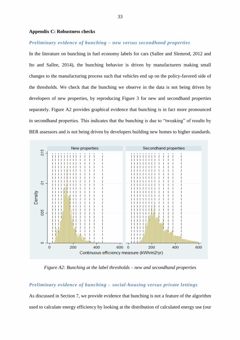
Preliminary evidence of bunching – new versus secondhand properties

In the literature on bunching in fuel economy labels for cars (Sallee and Slemrod, 2012 and

Ito and Sallee, 2014), the bunching behavior is driven by manufacturers making small

changes to the manufacturing process such that vehicles end up on the policy-favored side of

the thresholds. We check that the bunching we observe in the data is not being driven by

developers of new properties, by reproducing Figure 3 for new and secondhand properties

separately. Figure A2 provides graphical evidence that bunching is in fact more pronounced

in secondhand properties. This indicates that the bunching is due to “tweaking” of results by

BER assessors and is not being driven by developers building new homes to higher standards.

Figure A2: Bunching at the label thresholds – new and secondhand properties

Preliminary evidence of bunching – social-housing versus private lettings

As discussed in Section 7, we provide evidence that bunching is not a feature of the algorithm

used to calculate energy efficiency by looking at the distribution of calculated energy use (our

34

measure of energy efficiency) where, we believe, the assessors do not have an incentive to

adjust the energy efficiency score, i.e., for properties designated for social housing. We

compare this distribution to that of private lettings where it is likely that incentive to bunch

do exist.

Figure A3: Distribution of energy efficiency Private and Social housing lettings

Figure A3 shows a stark contrast in the distribution of energy efficiency between social

housing and private lettings. While for social housing there does appear to be a discontinuity

at 300kWh/m2/yr; the cut-off between D2 and E1 labels, the discontinuities are much more

pronounced and more pervasive for private lettings.

Returns to energy efficiency for rural versus non-rural properties:

As noted in Section 3, the Central Statistics Office were not able to obtain an exact match

between all properties in the Property Price Register and BER datasets, and most of these

35

unmatched observations were for properties located in rural areas. We check that the results

of our hedonic regression model are not being affected by this by looking at the returns to

energy efficiency for rural and non-rural properties separately. As Table A2 below illustrates,

for highly-efficient properties (those that received an A or B1 rating) the returns are

somewhat larger once rural properties are excluded, this is likely due in part to the fact that

there are relatively few highly-efficient properties located in rural areas (for example, there

are only 43 A-rated properties located in rural areas). Therefore, our results presented in

Table 4 are likely to be a lower-bound estimate of the returns to energy efficiency at the top

of the efficiency scale. However, lower down the scale the returns in rural and non-rural

properties are comparable. Therefore, we do not believe that our results are significantly

affected by these missing properties.

Table A2: Effect of BER labels on transaction prices, rural and non-rural properties:

Y: log (Price ex.VAT) Rural properties Non-rural properties

A (aggregated) 0.117(0.074) 0.251(0.024)***

B1 0.131(0.069)* 0.196(0.020)***

B2 0.142(0.043)*** 0.138(0.013)***

B3 0.172(0.028)*** 0.118(0.009)***

C1 0.130(0.025)*** 0.135(0.008)***

C2 0.151(0.024)*** 0.141(0.008)***

C3 0.171(0.023)*** 0.152(0.007)***

D1 0.140(0.023)*** 0.137(0.007)***

D2 0.131(0.023)*** 0.133(0.007)***

E1 0.132(0.025)*** 0.115(0.007)***

E2 0.117(0.024)*** 0.121(0.007)***

F 0.083(0.025)*** 0.079(0.007)***

G Reference Reference

Observations 61,561 13,140

R-squared 0.777 0.451 Notes: Robust standard errors in parentheses. *** p<0.01, ** p<0.05, * p<0.1.

Sensitivity to the order of the polynomial – bunching estimates:

The results displayed in Figure 4 and in Table 3 are based on an estimated polynomial

of degree 5. A polynomial of degree 5 was chosen as it led to the lower Akaike Information

Criterion (AIC) values than lower-order polynomials, and when model was estimated using

36

higher-order polynomials, the higher polynomials were frequently dropped due to

collinearity. Table A3 below shows that while the order of the polynomial does affect the

relative bunching estimates, the effect is not large and in all cases the pattern and significance

of the results are unchanged.

Table A3: Sensitivity to the order of the polynomial:

Relative bunching estimate ( )

Threshold P=3 P=4 P=5 P=6

A3 - B1 2.27 (0.70)*** 2.83 (0.89)*** 2.52 (0.87)*** 2.40 (0.82)***

B1 - B2 0.67 (0.10)*** 0.48 (0.09)*** 0.48 (0.08)*** 0.49 (0.09)***

B2 - B3 1.49 (0.24)*** 0.84 (0.19)*** 0.80 (0.18)*** 0.90 (0.18)***

B3 - C1 1.88 (0.32)*** 1.41 (0.24)*** 1.40 (0.25)*** 1.47 (0.27)***

C1 - C2 1.21 (0.17)*** 1.02 (0.18)*** 1.02 (0.19)*** 1.01 (0.19)***

C2 - C3 1.28 (0.22)*** 1.04 (0.19)*** 1.04 (0.19)*** 1.02 (0.19)***

C3 - D1 2.28 (0.34)*** 2.31 (0.45)*** 2.35 (0.45)*** 2.33 (0.45)***

D1 - D2 1.06 (0.10)*** 1.04 (0.12)*** 1.03 (0.10)*** 1.04 (0.11)***

D2 - E1 3.38 (0.55)*** 3.20 (0.72)*** 3.29 (0.71)*** 3.29 (0.73)***

E1 - E2 0.81 (0.09)*** 0.80 (0.11)*** 0.79 (0.11)*** 0.79 (0.11)***

E2 – F 2.18 (0.14)*** 2.25 (0.15)*** 2.23 (0.15)*** 2.22 (0.14)***

F – G 4.27 (0.12)*** 3.96 (0.18)*** 3.10 (0.18)*** 2.66 (0.16)***

Sensitivity to the excluded range – bunching estimates:

As the lower bound of the excluded range ( ) was determined visually, we

recalculate the bunching estimates firstly by widening the excluded range (i.e., making

lower) and then by narrowing it (i.e., making higher), both times by one bin (i.e.,

1/kWh/m2/year). A narrower bin should provide lower estimates of bunching and, as Table

A4 shows, this is what we find. Across some thresholds there are notable differences in the

bunching estimates when we vary the excluded range. However, comparing the estimates

from the narrow range (i.e., the most conservative estimates) to our main estimates (presented

in Table 3), the differences are never statistically significant. Therefore, we conclude that our

estimates are not biased by the choice of the excluded range.

37

Table A4: Sensitivity to the excluded range:

Relative bunching estimate ( )

Threshold reduced by 1 (wider excl. range) increased by 1 (narrower excl. range)

A3 – B1 2.62 (1.30)** 1.52 (0.48)***

B1 – B2 0.53 (0.15)*** 0.47 (0.08)***

B2 – B3 1.22 (0.28)*** 0.63 (0.11)***

B3 – C1 1.57 (0.36)*** 1.07 (0.16)***

C1 – C2 1.39 (0.26)*** 0.95 (0.10)***

C2 – C3 1.36 (0.26)*** 0.91 (0.11)***

C3 – D1 2.22 (0.40)*** 1.95 (0.22)***

D1 – D2 1.08 (0.10)*** 0.72 (0.05)***

D2 – E1 3.24 (0.49)*** 2.61 (0.31)***

E1 – E2 0.79 (0.10)*** 0.51 (0.05)***

E2 – F 2.62 (0.20)*** 1.72 (0.10)***

F – G 4.21 (0.17)*** 3.66 (0.13)***

Testing for buyer awareness of bunching:

As a final robustness check, we test whether property buyers may be aware of bunching

behavior and thus disregarding (or valuing less) the energy efficiency of properties if the

continuous measure of energy efficiency (the calculated energy use score) is near a label

threshold. To do so we run the hedonic model excluding properties with continuous energy-

use scores within 5 kWh of the favorable side of the threshold. Table A5 presents the results

from this subsample and for all properties; it shows that the estimates are not sensitive to the

exclusion of the observations near the thresholds.

Table A5: Hedonic regression results – testing for buyer awareness of bunching:

Y: log (Price ex.VAT) Baseline Excluding properties at/near the thresholds

A (aggregate) 0.229(0.023)*** 0.240(0.026)***

B1 0.180(0.020)*** 0.168(0.022)***

B2 0.128(0.013)*** 0.135(0.016)***

B3 0.123(0.009)*** 0.116(0.011)***

C1 0.125(0.008)*** 0.122(0.009)***

C2 0.136(0.008)*** 0.137(0.008)***

C3 0.151(0.007)*** 0.152(0.008)***

D1 0.135(0.007)*** 0.136(0.008)***

D2 0.132(0.007)*** 0.132(0.007)***

E1 0.119(0.007)*** 0.121(0.008)***

E2 0.123(0.007)*** 0.123(0.007)***

F 0.081(0.007)*** 0.082(0.007)***

G Reference Reference

Observations 74,701 60,046

R-squared 0.729 0.734 Notes: Robust standard errors in parentheses. *** p < 0.01, ** p < 0.05, * p < 0.1.