THE EFFECT OF ELECTORAL COMPETITIVENESS ON

INCUMBENT BEHAVIOR∗

Sanford C. GordonNew York University

Gregory HuberYale University

Abstract

What is the marginal effect of competitiveness on the power of electoral incentives? Ad-

dressing this question empirically is difficult because challenges to incumbents are endogenous

to their behavior in office. To overcome this obstacle, we exploit a unique feature of Kansas

courts: fourteen districts employ partisan elections to select judges, while seventeen employ

noncompetitive retention elections. In the latter, therefore, challengers are ruled out. We find

judges in partisan systems sentence more severely than those in retention systems. Additional

tests attribute this to the incentive effects of potential competition, rather than the selection of

more punitive judges in partisan districts.

∗This is the latest in a series of joint papers by the authors; the ordering of names reflects aprinciple of rotation. We thank Neal Beck, Alan Gerber, Catherine Hafer, Shigeo Hirano, DimitriLanda, David Mayhew, Rebecca Morton, Peter Rosendorff, Howard Rosenthal, Jasjeet Sekhon,Alastair Smith, Rocio Titiunik, Lynn Vavreck, Craig Volden, Ebonya Washington and the refereesand QJPS editors for their helpful comments. Earlier versions of this paper were presented atthe 2005 annual meeting of the Midwest Political Science Association and in seminars at Berkeley,the Harris School, NYU Law School, and Princeton, where we received valuable feedback. NicoleSimonelli provided excellent research assistance. This research was supported by the NationalScience Foundation (SES Grants 0317667 and 0318033). Gordon also gratefully acknowledges thesupport of the Center for the Study of Domestic Politics at Princeton, where he was in residencein 2005-2006.

1 Introduction

In empirical studies of the agency relationship between voters and elected officials, it has been well

established that the behavior of the latter seems in many cases to conform to the demands of the

former (e.g. Besley and Coate 2003; Bartels 1991; Miller and Stokes 1963). This conformity has

been explained with reference to the success of voters at selecting likeminded officials and by the

incentive effects of periodic review. To the extent that incumbents alter their behavior in anticipa-

tion of possible sanction at the polls, a puzzle emerges: To what extent does the competitiveness of

the electoral environment increase the power of these incentives? This question has taken on par-

ticular importance in the American political context, where public officials in numerous positions

frequently run for reelection unopposed or face only token opposition (Cox and Katz 1996).

The absence of serious challengers may be said to contribute to an erosion of democratic ac-

countability. At the same time, however, this absence (and the resulting lopsided margins by which

incumbents often retain office) may reflect incumbent compliance with public demands rather than

autonomy from them. In addition to serving as alternatives for voters, serious challengers in com-

petitive elections can audit incumbents and provide information to voters about the qualifications

of incumbents or their behavior in office. The mere threat that a challenger could play these roles

might be sufficient to alter incumbent behavior. Such a response would deny challengers a strong

case to make to voters for the incumbent’s replacement, or deter them from running altogether. In

this regard, the potential for competition could improve incumbent compliance because of the role

that challengers might play, but, in the vast majority of circumstances, never get the chance to.

A central empirical implication of this argument is that incumbents should be more responsive

to public demands when the potential for electoral competition is higher. Unfortunately, isolating

the effect of competitiveness empirically is difficult because challenger viability – whether in primary

or general election contests – is itself endogenous to incumbent performance. In other words, the

spirited electoral contests that officeholders fear are the very ones in which a challenger has a case

to make to voters about an incumbent’s failures.

To overcome this problem, we rely on a unique feature of district court judicial elections in

Kansas. There, fourteen judicial districts employ partisan competitive elections to select judges,

while seventeen employ gubernatorial appointment and non-competitive retention elections. The

retention districts provide an appropriate baseline of comparison: Although judges in those districts

must face the voters, by law, there can be no challengers. Comparing officials in a single state

permits us to hold constant numerous potential confounding factors, most importantly the legal

environment in which those officials operate.

We derive predictions concerning the relationship between the sentencing behavior of incum-

bent judges and the electoral system in which they operate. Employing data on felony convictions

in Kansas and several econometric approaches, we demonstrate that judges in partisan competitive

systems sentence significantly more punitively than those in retention systems. Our identification

strategy subsequently exploits variation in judges’ electoral calendars to demonstrate that the effect

of the electoral system is more pronounced in altering judges’ incentives than in changing who is

selected to office. Our findings demonstrate that the potential for competition from challengers

substantially enhances incumbent attention to voter demands, while providing insight into both

the functioning of electoral systems generally and the operation of the criminal justice system in

particular.

2 Elections, Accountability, and the Role of Challengers

2.1 Selection and Incentives

Broadly speaking, there are two mechanisms by which elections might produce faithful representa-

tion on the part of elected officials. The first is selection. Ideally, competitive elections allow voters

to choose candidates whose preferences most closely mirror their own (Downs 1957; Fearon 1999).

In the selection account, the presence of challengers facilitates a closer match between voters and

their representatives through the provision of alternatives. The second mechanism is the incentive

effect of elections (Barro 1973; Ferejohn 1986). Even those incumbents who do not share their

constituents’ preferences or possess strong qualifications may nonetheless behave faithfully or work

hard if their failure to do so will result in their subsequent punishment at the polls.1

1Of course, faithful agency by politicians to their constituents, while individually rational, mightlead to collectively suboptimal results (e.g. Mayhew 1974; Maskin and Tirole 2004). We return tothis general point in the conclusion.

2

2.2 The Functions of Challengers

The threat a challenger poses to an incumbent plays a critical role in structuring incumbent in-

centives. If voter preferences are heterogeneous, the presence of an additional choice on the ballot

may be sufficient to reduce the vote share of an incumbent with an otherwise strong reputation.

Challengers also play an informational role in elections. They are strongly motivated to audit

incumbent performance and, when possible, publicize actual or perceived missteps (Arnold 1993).

In this respect, challengers play a “fire alarm” role (McCubbins and Schwartz 1984), monitoring

incumbents on behalf of voters and reporting evidence of shirking. This role complements the infor-

mational function of the media, constituency groups, and grassroots organizations, as attention to

incumbent behavior is far more intense during competitive electoral contests (Arnold 2004; Alvarez

1997). If entering a race entails opportunity costs for a challenger, the very fact that he or she has

stepped into the ring may signal to voters that the incumbent is deficient in some regard (Gordon,

Huber, and Landa forthcoming).

What should we expect to observe if incumbents alter their behavior in anticipation of this

threat? First, we should frequently see races lacking a viable challenger. Viability is often a

consequence of the incumbent’s vulnerability, which he or she will take pains to minimize.2 In

the absence of viable challengers, incumbents should secure reelection by wide margins. Second,

we should expect voters to be ignorant much of the time, because their knowledge of incumbent

behavior is endogenous to campaigning by challengers (and the subsequent attention paid by the

media).

In light of these difficulties, efforts to ascertain the incentive effect of electoral competition

using data on voter knowledge and election outcomes will likely suffer from simultaneity bias.

One might posit, for example, that a relationship between competition and compliance implies

that unpopular decisions by elected officials will tempt challengers to enter a race, lowering an

incumbent’s vote share (cf. Brady, Canes-Wrone, and Cogan 2002). However, incumbents who

make unpopular decisions may perceive themselves to be safe from effective challenges for reasons

the analyst cannot observe. Similarly, one could argue that low levels of voter knowledge ought to

2When we do observe viable challenges, it is likely due to unanticipated shocks that makeincumbents vulnerable, actions by incumbents unwilling or incapable of heeding public opinion,shifting electoral coalitions that make extant majorities difficult to sustain, or entrenched ideologicaldivisions in a district.

3

be associated with greater incumbent noncompliance because voter ignorance allows incumbents to

make choices without electoral implications. However, low levels of voter knowledge or attentiveness

may be a consequence of incumbent compliance with voter demands and its deterrent effect on

challenger entry, rather than a cause of noncompliance.

A more promising direction is to examine the behavior of incumbents. In particular, incum-

bents should alter their behavior given the threat of real electoral competition more than they

would in its absence. Moving toward an empirical test of this prediction requires surmounting two

obstacles. First, we require a measure of the extent of incumbent compliance with public demands.

Second, to overcome the endogeneity of challenger viability, we require an exogenous determinant

of the potential threat of electoral competition.

2.3 The Case of Judicial Elections

Examining the behavior of trial judges is an especially useful means for understanding the connec-

tion between electoral institutions and the behavior of public officials. Examining the behavior of

Kansas trial court judges in particular provides a unique opportunity to understand the specific

effects of electoral competitiveness.

The behavior of elected trial judges. Trial judges must face periodic review by voters in

39 American states. Examining their behavior, as opposed to that of other elected officials, confers

three immediate advantages. First, we can employ the sentences sanctioned by judges in individual

criminal cases to obtain a direct measure of action that is comparable across officials and different

institutional contexts. Owing to reporting requirements, data on sentencing is often accompanied

by an enormous volume of information about specific conditions under which sentences were handed

down. This makes it possible to account for much of the natural heterogeneity of circumstances

judges confront when making decisions.

Second, voters tend to know next to nothing about judges’ decisions in the vast majority

of cases (Mathias 1990; Sheldon and Lovrich 1983). To the extent that very low levels of voter

knowledge enhance opportunities for incumbent autonomy, the study of elected judges comprises a

difficult case for testing general theories of electoral accountability.

Third, on the rare occasion that voters do become aware of judicial behavior, it is usually due

to coverage of high-profile trials or controversial cases of recidivism. Critically, adverse publicity

4

nearly always corresponds to cases of perceived judicial leniency. Media accounts of courtroom

proceedings tend to result in voters believing judges are too lenient (Roberts and Edwards 1989).

Additionally, voters are inclined to believe the criminal justice system as a whole is too lenient

(Warr 1995). Finally, nearly all convicts claim to have been punished too much, and more definitive

evidence of overpunishment typically comes to light years after a judge hands down a sentence.3

By contrast, an episode of recidivism or unusually pointed criticism of a judge by a victims’ rights

group or police union (or challenger) provides a more immediate signal that a judge’s sentence did

not fit the crime.

An informational environment in which judges have greater reason to fear voters perceiving

them as too lenient than too severe (if they perceive judges at all) creates an asymmetry: If the

constraint of public opinion binds at all, it will tend to make judges weakly more punitive rather than

more moderate with respect to constituent preferences (Huber and Gordon 2004). This asymmetry

is reinforced by an important feature of the trial judge’s institutional environment: sentencing

guideline regimes and statutory maximum penalties imply that those sentences a typical voter

might perceive as “too harsh” often fall outside the range of the judge’s discretion.4

The (weak) unidirectionality of the electoral incentive is valuable because it eliminates the

need for the analyst to determine which direction (more lenient or harsh) engenders greater compli-

ance with public demands for a particular judge, a difficulty that besets the analysis of legislative

behavior (but see Lee, Moretti, and Butler 2004).5 This is critical because in general we will not

be able to obtain a measure of a judge’s primitive sentencing preferences apart from those induced

by his or her political environment.

Kansas judicial selection as a natural experiment. There are 31 judicial districts in

Kansas, each composed of from one to seven of the state’s 105 counties. Incumbent judges occupy

unique seats (called “divisions”), and are therefore not in direct competition with one another.

3Moreover, even evidence of wrongful prosecution or juror error attaches not to the sentencingjudge, but rather to those who fabricated evidence or misjudged its veracity.

4Whereas all crimes have mandatory maximum penalties, not all have mandatory minima. Inmany states (including Kansas, the subject of our analysis below), guideline minimum sentencesmay be broached if the judge determines the presence of exculpatory factors.

5In the context of sentencing, the bidirectionality problem is most likely to emerge given voterevaluation of sentences for so-called “victimless crimes” such as drug possession. Accordingly, weexclude sentences for such crimes in our analysis below.

5

Judges in all districts serve staggered four year terms, with elections occurring in even years.

Kansas is one of two states in which the method of selecting judges differs from district to district.

Since 1974, subject to approval in a district-wide referendum, individual districts can choose to

replace the default system of selecting judges via partisan competitive elections with a system of

gubernatorial appointment and non-competitive retention elections.

A brief history of the adoption process is warranted. A 1972 amendment to the state con-

stitution authorized the legislature to codify procedures for districts to choose between the two

selection methods. Once those procedures were in place, each existing judicial district voted on its

own selection method in 1974. That year, 23 of the 29 districts switched to retention elections.

Since then, in order to place the issue of judicial selection system on the general election ballot,

supporters must present a petition signed by more of a district’s voters than 5% of the number

who voted in the preceding secretary of state election. Since 1984, a statutory provision prohibits

a district from returning to this question more than once every seven years.

By 1984, eight of the districts that initially switched to retention had returned to the partisan

method (and two new retention districts were created out of counties in existing ones). Three

additional districts voted to keep the retention system, although one subsequently returned to the

partisan method. In 1986, the district encompassing Kansas City unsuccessfully voted to shift

back to the retention system it had narrowly abandoned in 1980, while two other districts (one

containing Topeka, and the other a northern suburb of Kansas City) failed to shift from retention

to the partisan method in 2000. Since then, no additional measures have been considered, although

some groups have pressed to eliminate one option or the other altogether (Sanders 1995; Kansas

Citizens Justice Initiative 1999; Ventimiglia 2006). The most recent observed vote in favor of the

retention method ranges from 26% to 68%, with a mean of about 50%.6

In districts employing the partisan selection method, judges seek their party’s nomination

in primaries held in August.7 The victors then face off in a general contest on Election Day

6Source: State of Kansas, Election Statistics: Primary and General Elections. Because districtswere reorganized between 1974 and 2006, we identified the most recent vote on selections systems ineach county during this period, and then aggregated these data by contemporary judicial districtsto calculate these percentages. Reweighting the county level data to adjust for shifts in relativepopulation produces highly similar figures.

7The partisan primaries are closed to members of the opposite party, although the Democraticprimary is open to unaffiliated voters.

6

in November.8 In retention districts, a nominating commission in each proposes names to the

governor.9 If she chooses to appoint a nominee, that judge will serve a one-year probationary

term followed by a retention vote.10 If retained, the judge will stand for retention every four years

thereafter. In a retention election, the judge’s name appears on the ballot, and voters can vote

“Yes” or “No.”11 A map of the judicial districts appears in Figure 1. Fourteen districts currently

employ the familiar partisan selection method. These districts comprise 53 counties, in which

roughly 42% of Kansans reside. The remaining seventeen districts employ the non-competitive

retention method.

Figure 1 about here

Assuming that a district’s choice of method for selecting judges is unconfounded by factors that

influence judicial decision making (discussed in greater detail below), the institutional variation in

Kansas judicial districts permits us to consider the incentives for incumbents created by the threat

of challengers, while circumventing the problem of endogenous challenger viability. Whereas the

threat posed by challengers in the primary or general election may vary among competitive districts,

in retention districts there can be no challenger irrespective of incumbent behavior in office. The

set of decisions made by judges in retention districts therefore constitutes a suitable control group

against which to make comparisons of decisions made by judges who serve under the threat of

primary and/or general election challenges.

Other empirical contexts in which these comparisons might be made are problematic. One

could, for example, consider comparing judicial sentencing behavior across states with different

selection methods. Even if one could adequately control for the contextual and institutional het-

8We compiled data on the 138 contests in partisan competitive districts involving an incum-bent trial judge from 1994 to 2002 (source: Kansas Secretary of State). Nine incumbents facedchallengers in primary elections (three lost) and ten did so in general elections (one lost). As wenoted above, because challenger entry is endogenous to incumbent performance, these numbers bythemselves do not indicate an effect on incumbent accountability, although they do reveal thatincumbent judges can be defeated.

9Commissions are each composed of an equal number of attorneys and no attorneys. Attorneymembers are elected by their peers; others are appointed by Boards of County Commissioners.

10In the absence of an appointment, the seat remains open.11From 1994 to 2002, 144 judges stood for retention election; none lost his or her seat. The average

Yes vote for incumbent judges was 76% (with a standard deviation of 5%) and the minimum was51%.

7

erogeneity across states, however, fundamental differences in legal systems would remain difficult to

account for. Criminal codes vary enormously in how they categorize crimes, and judges in different

states have vastly different discretion in punishing offenders. By confining our analysis to a single

state, we can hold constant the legal system under which judges (as well as prosecutors, defense

attorneys, and defendants) operate.

Another possibility is to examine the behavior of officials in another state. For example, Mis-

souri has a similarly bifurcated system of selecting judges. However, Missouri adopted nonpartisan

selection of circuit court judges only in urban areas (Kansas City and St. Louis) on the heels

of charges that urban political machines were exercising undue influence in the selection process

(Watson and Downing 1969). The effect of the selection mechanism in Missouri is therefore not

separable from numerous other differences between urban and rural counties. Such confounding

influences are likely to be minimal in the Kansas setting. Two of the four most urban counties in

the state (Wyandotte and Sedgwick) select district judges via partisan races, while the other two

(Shawnee and Johnson) employ a retention system. Rural counties are similarly split.

To determine whether the institutional variable is a proxy for other features of judges’ envi-

ronments (e.g. voter preferences, engagement, or attentiveness), we gathered data on the political

and demographic characteristics of Kansas’ 31 judicial districts. We then compared the charac-

teristics of the partisan competitive and retention districts using t-tests of equality of means and

bootstrapped Kolmogorov-Smirnov tests of equality of distributions. The first two columns of Table

1 report the associated p-values. District crime rate is one of two variables for which substantial

imbalance exists between the two systems – retention districts have significantly higher crime rates,

a result largely driven by Shawnee County (the location of Topeka). The other variable is the aver-

age support for Kansas Supreme Court justices in their retention elections, which could conceivably

proxy citizen mistrust of the judicial system. This imbalance appears because of very low support

for incumbent Supreme Court judges in Districts 4 and 11.

Table 1 about here

8

2.4 Identification Strategy

In Appendix A, we present a simple heuristic model to clarify the intuition underlying the incentive

effect of potential competitiveness on elected judges. We anticipate that, ceteris paribus, incumbent

judges in Kansas’s partisan competitive districts will sentence more punitively than judges in its

retention districts. While consistent with an incentive effect, such a finding would also be consistent

with a selection account: voters in partisan districts may select inherently more punitive judges

than judicial nominating commissions do in retention districts. Alternatively, voters in partisan

districts may elect district attorneys more punitive than voters in retention districts do.

Addressing the concern about differences in elected prosecutors is straightforward and is dis-

cussed in greater detail below. Our strategy for identifying the incentive effect of potential compet-

itiveness, and for eliminating rival interpretations for that effect, proceeds in several phases. The

first two aim to ensure that the distinction between electoral systems is not merely a proxy for

other features of districts that may contribute to differences in sentencing. Phase one is regression-

based: we consider whether the estimated effect of the electoral system is sensitive to the inclusion

of observable district characteristics, including the crime rate and electoral support for incumbent

Supreme Court judges, in a saturated model of sentencing behavior.

Phase two relaxes the parametric assumptions of regression in a matching analysis. We com-

pare outcomes from similar criminal cases drawn from matched pairs of observably similar judicial

districts with different electoral systems. This approach discards data from retention districts that

are not comparable to those that employ the competitive system. We then conduct an additional

matching analysis restricting our attention to districts for which the most recent referendum on

selection mechanism was “close” (defined below). The intuition behind this approach (see Lee

forthcoming) is that districts where support is near-even are those in which random factors affect-

ing turnout (which is quite low for these referenda) will tend to play a prominent role relative to

underlying voter preferences, thereby more closely approximating a randomized experiment.

Of course, the possibility still remains that the incentive effect of the electoral system is

confounded by an unobservable tendency of partisan competitive districts to select inherently more

punitive judges. Our strategy for disentangling these competing explanations for differences in

judicial behavior (Phase three) exploits variation in behavior over judges’ electoral calendars. If

9

elected judges discount the future value of holding office relative to the benefit of assigning their

most preferred sentences, then an incentive-based account predicts that judges will sentence weakly

more punitively as election approaches, controlling for secular trends in sentencing. We refer to

this phenomenon as the electoral “proximity effect.”12 A pure selection account, by contrast, is

incompatible with the dynamic adjustment implied by a significant proximity effect.

More importantly, considering the nature of the interaction between electoral rules and elec-

toral proximity sheds additional light on how judges’ incentives operate. Suppose that electoral

incentives were comparable under both selection methods, but that voters in partisan competi-

tive districts tended to select judges who were inherently more punitive than those selected by

nominating commissions in retention districts. We should then anticipate the electoral proximity

effect to be smaller in the competitive districts than the noncompetitive ones. The intuition is

as follows: at any given point on the electoral calendar, retention judges would sentence more le-

niently on average than partisan judges. Given diminishing electoral returns to sentencing harshly,

the marginal electoral benefit to a retention judge of increasing her sentence would be larger. As

election drew closer, the retention judge would therefore respond to a shift in her priorities toward

accommodating electoral pressure with larger increases in sentencing than would a partisan judge.

By contrast, suppose judges did not differ much in their innate sentencing preferences across

selection systems, but that partisan competitive incumbents were instead responding to the threat

of a viable challenger with more punitive sentences. This account is consistent with either a smaller

or larger proximity effect in partisan competitive districts than in retention districts. Judges in

partisan competitive systems are more likely to be constrained by statutory or guideline maximum

sentences earlier in their terms than their retention system counterparts. Consequently, situations

may arise in which a partisan judge’s sentencing is unresponsive to electoral proximity whereas

a retention judge’s sentencing continues to increase over the course of her term. Unconstrained

12For two reasons, it is appropriate to view electoral proximity as exogenous to judicial decisionmaking. First, pursuant to Rule 107 of the Kansas Supreme Court, trial court cases must beapportioned “as equally as possible” among judges within a district, and judges cannot refusecases except in instances of clear conflicts of interest. The practical effect of this rule has beenthe adoption of random or near-random assignment of cases across judges within the districts.Consequently, judges cannot “cherry pick” cases they expect to be politically uncontroversial, norcan prosecutors or defense attorneys cherry pick judges on the basis of their electoral proximity.Second, the electoral calendar is fixed, so judges cannot call early elections to capitalize on populardecisions.

10

partisan judges, however, face higher marginal electoral benefits from sentencing harshly at any

given point in their electoral calendars (to avoid the threat of a viable challenger); consequently,

as election draws closer (and electoral benefits weigh more heavily in their decision calculus),

partisan competitive judges would respond with larger increases in sentencing than their retention

counterparts.

To summarize the third phase of our strategy: (1) A finding that at least some judges become

more punitive as election approaches is consistent with an account based on electoral incentives

and not selection alone; (2) A finding that this electoral proximity effect is greater in retention

districts than partisan competitive districts is consistent with both the challenger-based incentive

mechanism and the alternative, selection-based account; (3) A finding that the proximity effect is

greater in partisan competitive districts than retention districts is consistent with the challenger-

based incentive mechanism but not the selection account.

3 Data and Method

3.1 Sentencing in Kansas

We obtained data on the sentencing behavior of 160 Kansas district court judges from 1997 to

2003. Seventy-three judges served in districts with partisan competitive elections, and eighty-seven

in districts with retention elections.13 Criminal sentencing in Kansas is governed by the Kansas

Sentencing Guidelines Act of 1993 as amended (hereafter, the guidelines), which places limits on

the discretion of trial court judges in assigning sentences to convicted offenders. Convicts serve at

least 85% of the sentence a judge hands down before becoming eligible for parole. As with most

guideline systems, judges are required to take into account an offender’s criminal history and the

severity of the offense committed to determine an applicable range of appropriate sentences. Judges

then have limited discretion to depart from the recommended range.

Although the guidelines suggest a single, presumptive sentence for history/severity combina-

tions, judges can generally choose to assign any sentence between the minimum and maximum

guideline sentences without further justification. If a judge wishes to “upwardly depart,” he or

13Some districts also have magistrate judges, who have limited authority and whose decisions areexcluded from our analysis.

11

she may assign a sentence up to twice the guideline maximum given one or more aggravating cir-

cumstances specified in the statute.14 He or she may also assign a departure sentence below the

minimum sentence given mitigating circumstances.15 Departure sentences are subject to appellate

review and will be sustained if there are “substantial and compelling reasons for the departure.”16

In multiple count convictions, judges have discretion to assign sentences on less severe counts to

run either concurrently or consecutively to the first sentence with the condition that the total time

in prison cannot exceed twice the sentence on the primary count.

The dataset for our analysis was created by merging information about Kansas’s judges and

judicial districts with records of the sentences they assigned to individual defendants collected by

the Kansas Sentencing Commission. We restricted our analysis to those felonies for which there were

a reasonable number of cases across the state (more than 250), for which judges have discretion in

sentencing, and for which incarceration is a possibility. This left us with a range of person (assault,

criminal threat, robbery, sexual assault) and property crimes (theft, burglary, arson).17 We have

18,141 cases for the period between July 1, 1997 and June 30, 2003.18

The vast majority of cases were resolved via plea bargain. This is similar to the situation

in most states, and does not threaten our ability to make inferences about judges’ incentives. A

judge’s optimal sentence (discounted by the probability of a conviction) is properly viewed as a

reversion or threat point in the negotiation between the prosecutor and defendant. Also, judges in

14Prior to the Kansas Supreme Court’s decision on May 25, 2001 in State v. Gould (271 Kan.394, 23 P.3d 801), judges were free to identify those aggravating factors that warranted a departureabove the guideline maximum sentence. The Gould decision held that any facts that led a judgeto assign a sentence above the guideline maximum would have to be proven “beyond a reasonabledoubt” before a jury. In a measure that became effective June 6, 2002, the state legislature alteredthe guidelines to require such factors be proven to a jury, either during trial or in a separatepost-conviction sentencing hearing. In our analysis, we account for how this ruling, in the periodbetween May 2001 and June 2002, limited judges’ authority to sentence single count cases to nomore than the guideline maximum and multi-count cases to no more than twice that quantity.

15The Gould decision did not affect these downward departures.16See K.S.A. 22-3604.17We excluded homicide cases for two reasons. First, under Kansas law, judges lack sentencing

discretion for murder convictions. (The jury decides between life imprisonment and the deathpenalty.) Second, defendants often plead guilty to manslaughter to avoid a murder trial. (Includingthe manslaughter cases does not affect our main results.) Additionally, we excluded drug crimes onthe grounds that preferences about punishment for drug offenders may vary substantially, whereaspunishment for those convicted of the crimes we examine is uncontroversial. See also footnote 5.

18We discard all cases heard by judges who sentenced fewer than 25 cases in our dataset and allcases heard by retention judges during their probationary term.

12

Kansas have the discretion to reject settlements between prosecutors and defendants.19 Because

bargaining takes place in the shadow of the judge (LaCasse and Payne 1999), it incorporates the

judge’s underlying preferences about punishment.20 Observed sentences range from zero to 3,185

months. In 69% of cases, the sentence includes probation, a fine, or community service, but no time

in prison. For the remaining 31% of cases, the median prison sentence is 32 months. The number

of counts in a conviction ranges from one to 50. 74% of cases have only a single count, and 99%

have five or fewer counts.

A cursory examination of the data reveals preliminary support for the hypothesis that sen-

tencing in partisan competitive districts is more severe than in retention districts. 35% of sentences

handed down in the competitive districts include prison terms, compared with 27% in the retention

jurisdictions. Likewise, the median non-zero prison sentence is higher in the partisan than reten-

tion districts — 33 versus 31 months. The respective average non-zero prison terms are 66 and 57

months. All of these differences are highly statistically significant.

3.2 Case-level Covariates

A downside to a simple description of mean differences in sentencing outcomes is that this approach

does not account for other relevant distinctions among cases. Fortunately, we have numerous vari-

ables to account for contextual heterogeneity in sentencing. Summary statistics for model variables

appear in Table 2. Our primary measure of culpability is the natural log of the presumptive sen-

tence (plus one, to match the scaling of the dependent variable) associated with the conviction’s

top count. This captures the extent to which the state’s elected officials view that criminal act by a

defendant with a particular criminal history as harmful. We also include two indicator variables to

control for revisions to the guidelines that occurred in 1996 and 1999.21 Because judges have discre-

tion to sentence additional counts concurrently or consecutively (subject to constraints discussed

above), we also control for the number of additional counts in the conviction. Aggravating factors

19Note that the fact that judges rarely reject plea bargains is not evidence against a judge’sinfluence in the process; if attorneys correctly anticipate what a judge will accept, we should neverobserve plea bargains rejected.

20Confirming the judge’s importance, we find substantial variation in sentencing practices indistricts with multiple judges but only one district attorney.

21Earlier guideline regimes are relevant because the applicable guidelines are those in place atthe time of the felony, not the sentencing.

13

the judge is obliged to take into account include whether the defendant is a classified persistent sex

offender, whether he or she was in possession of a firearm at the time of the crime, and whether

the victim was a child, government employee, or law enforcement official.

Table 2 about here

We also include crime-specific indicator variables to account for heterogeneity in sentences, and

year-specific effects to capture non-monotone secular trends in perceptions of criminal culpability.

These latter controls are also vital because we wish to account for the confounding effect of the

prosecutor’s electoral calendar. All district attorneys in Kansas are on the same four year electoral

calendar, but judges within a district serve staggered terms. Year effects therefore control for

changes in sentencing that might result from variation over time in prosecutors’ electoral incentives.

In our analysis of the judge’s electoral proximity effect, we can also account for average differences

in district attorneys’ offices through the inclusion of judge-specific fixed effects. These span all time-

invariant features of the district (including, for example, the culture in the prosecutor’s office).

Variables affecting punitiveness consist of defendant-, case-, and judge-specific characteristics.

Included in the model are indicators of whether the sentence resulted from a plea bargain and

whether the defendant had appointed counsel. We also include measures representing whether the

defendant was male, nonwhite, or Hispanic. We control for defendant age and age-squared (under

the hypothesis that judges are likely to be lenient toward both the youngest and oldest defendants).

An indicator variable equals one if the judge serves in a partisan competitive district, and zero if

in a retention district. (Our measure of electoral proximity is discussed below.)

4 Results

4.1 The Baseline Systemic Effect

Our first set of estimates concerns the baseline hypothesis: Ceteris paribus, judges should behave

more punitively in partisan competitive districts than in retention districts. We first present the

results of our regression estimation, and then proceed to the matching analysis.

Regression Analysis. Our regression analysis relies on two substantive assumptions. First,

all judges, no matter how lenient, adhere to the principle of proportionality : greater culpabil-

14

ity demands greater punishment. Second, from the perspective of the defendant, the worst non-

incarcerative sentence is preferable to the most lenient prison term. In Appendix B, we demonstrate

how these assumptions, coupled with the right-censoring implied by statutory maximum sentences,

yield the two-limit Tobit likelihood function (with an adjustment for judge-specific groupwise het-

eroscedasticity). The dependent variable is the natural logarithm of the prison term, in months,

plus an unidentified constant. We adopt the common practice of setting the constant to one.

This normalization implies that one month in prison is exactly twice as painful as the worst non-

incarcerative punishment. (We experimented with a broad range of alternative values, none of

which affected our results.) Finally, note that a left-censored observation corresponding to zero

prison time does not stand in for an unobserved “negative” sentence. All convicted felons are

punished, but many are punished with a sentence less severe than prison.

First, we estimated four Tobit models, the coefficient estimates from which appear in columns

1, 2, 4, and 5 of Table 3. Specifications (1) and (2) employ all observations. Specifications (4) and

(5) restrict the sample to all cases from retention districts plus cases from competitive districts in

which the judge faced no competition in the subsequent election. Restricting the sample in this

way is meant to capture the notion that it is the potential for challenger entry, rather than the fact

of a challenge, that motivates changes in the behavior of incumbents. Models (2) and (5) include

aggregate district-level measures in addition to case- and defendant-level factors.

Table 3 about here

We note a large number of significant predictors of punishment. The presumptive sentence

and additional counts on the conviction have very strong positive effects, as expected, as do the

aggravating factors. Also as expected, the presence of appointed (rather than privately-hired)

counsel raises the expected length of incarceration while a plea bargain lowers it. We further find

that nonwhites and Hispanics tend to receive larger punishments, even controlling for the legally

relevant characteristics of individual cases. These findings, while troubling, are beyond the scope

of the current analysis.

The column (2) and (5) specifications with district-level measures suggests more stringent

sentences in districts with larger nonwhite populations and higher turnout and crime rates. Finally,

likelihood ratio tests for all specifications allow us overwhelmingly to reject the null hypothesis that

15

the year-specific indicator variables are jointly insignificant.

Next, we turn to the effect of potential electoral competition. In the four specifications dis-

cussed above, as expected, the coefficient on the partisan competitive district indicator is positive

and highly statistically significant. Note that restricting our sample to judges who were subse-

quently unchallenged does not substantially alter the estimated effect of competitiveness. This

suggests that the results are not driven by the behavior of judges who, ex ante, perceive themselves

as particularly vulnerable.

Because the magnitude of Tobit coefficients can be difficult to interpret, we derived several

quantities of greater substantive interest. This entailed setting all control variables at their sample

medians (for district characteristics, we employ the district medians), and employing the modal

crime (burglary) and year (2001). Our findings suggest estimated differences in the probability

of an assigned prison term between partisan competitive and retention districts of 2.81% and

4.01%, depending on specification. These numbers may seem small at first, but one must keep

in mind that the baseline probability of incarceration with the control variables set in this way

is approximately 17% to 18% (depending on specification). The proportionate increase in the

probability of incarceration associated with a change in the electoral rules is therefore about 16%

to 23%, depending on specification.

Next, we calculated the change in the expected sentence given prison assignment (a more

meaningful quantity than the change in unconditional expected prison time). Here, we set the

value of the logged presumptive sentence equal to its median among observations for which prison

was imposed. We find that the presence of a potential challenger increases the expected non-zero

sentence by about 2.5 to 3.7 months, which represents a 7.8% to 11.6% increase over the median

non-zero prison sentence in a retention district (32 months).

While our dataset includes thousands of case-level observations, it would be erroneous to

assume that these observations are independent. We employ two approaches to test the sensitivity of

our results to violations of independence. The first is to cluster observations by group in calculating

the covariance matrix of our coefficient estimates. The standard errors reported in Table 3 are

clustered at the judge level. We also derived standard errors clustering at the judge-year, district-

year, and district levels. Regardless of the level at which the dependence is assumed to exist, we

can always reject the null hypothesis at a p-value of 0.03 or smaller (one-tailed test).

16

The clustering approach requires assuming that the number of groups approaches infinity,

which may not be merited if dependence among observations operates at the district level. As an

additional robustness check, we therefore employed the two-step approach advocated by Wooldridge

(2006, 19-20): First, estimate the Tobit specifications in columns (1) and (4), substituting a vector

of district-specific effects for the partisan selection indicator. Second, using weighted least squares,

regress the coefficient estimates for the district effects on the district-level measures, including the

selection method. (The weighting matrix has for its diagonal elements the ratio of the number

of observations specific to each district to the variance of the first-stage district effect estimate.)

Estimates for the second stage regressions appear in columns (3) and (6) of Table 3. In both

specifications, the effect of the partisan selection method on the conditional district mean is positive

and statistically significant at above the 95% level.

Matching. The Tobit models, while theoretically motivated, require strong functional form

assumptions (e.g. linearity in variables). To ensure these do not drive our results, we also analyzed

the data using a more flexible approach: nearest neighbor, one-to-one matching.22 Matching pro-

ceeds by pairing observations from treatment (partisan competitive) and control (retention) groups

that are similar in terms of their observed covariates, and comparing the outcomes (incarceration).

In the current application, the wealth of data permit us to obtain exact matches – and thus perfect

balance – in treatment and control groups on all discrete case, defendant, and crime characteristics

listed above. Given a group of exact matches, we pair observations closest in defendant age.23

Estimates for the matching analysis are displayed in Table 4. The table displays estimates

of average treatment effects on the treated (ATT), i.e. the estimated effect of the electoral system

on sentences administered in partisan competitive districts.24 For the ATT estimates in columns

(1) and (2), we make no effort to achieve balance on district-level observables. A case with a

particular fact pattern from a partisan competitive district may be matched with one with the

same fact pattern from any of the seventeen retention districts. The first row of estimates reports

ATT estimates of changes in the probability of incarceration. The highly statistically significant

22Matching was conducted using Sekhon’s (2006) Match algorithm in R.23When necessary, we employ a caliper to insure balance on age. The p-values for bootstrapped

Kolmogorov-Smirnov tests of equality of distributions after matching range from 0.23 to 0.93.24ATT estimates permit superior balance on covariates not exactly matched on (particularly at

the district level – see below), but are comparable to average treatment effect (ATE) estimates.

17

3.6% to 3.8% increase confirms the Tobit results.

Table 4 about here

The parametric assumptions underlying the Tobit specification permitted us to calculate the

expected change in incarceration given a prison sentence was imposed. The matching algorithm

does not permit us to derive a comparable figure without additional assumptions; however, by

pooling both prison and non-prison sentences, we can estimate the average treatment effect in

months across all observations. The expected shift – quite small because of the large number of

sentences with no prison time – is a still statistically significant 0.554 or 0.551 months, depending

on whether subsequently challenged judges are included.

Our ability to exactly match on discrete case factors stems from the fact that there are 1,134

unique fact pattern “clusters” in the sentencing data for which we possess observations from both

treatment and control groups. Distance matching on defendant age within each cluster without

concern of ties is expedited by the presence in the data of defendant birthdays, which allow us

to measure this characteristic to the day. Matching observations on the basis of district-level

variables is more complicated, owing to the presence of just 31 unique values for each measure.

This essentially guarantees the district-level covariates will not be balanced between treatment and

control groups at the case level, even if excellent balance can be achieved at the district level. We

therefore adopt a two-step approach. First, using the genetic matching algorithm of Diamond and

Sekhon (2005), we pair partisan competitive districts with politically and demographically similar

retention districts. For example, District 18 (Sedgwick County, the location of Wichita) is paired

with District 7 (Douglas County, the location of Lawrence). (The full list of district matches is:

13/6, 14/8, 15/12, 16/8, 17/12, 18/7, 19/7, 20/30, 22/12, 23/30, 24/12, 26/25, 27/21, and 29/7.)

Post-matching balance statistics at the district level appear in the third and fourth columns of

Table 1. Note that this technique enables us to achieve balance on the crime rate and Supreme

Court retention vote, both of which were significantly unbalanced in the raw district-level data.

Having matched comparable districts, we then search for unique fact pattern clusters in district

pairs, matching observations closest in age as above.

Results from the analysis with district matching appear in the third and fourth columns

of Table 4. The district matching technique discards a large volume of sentencing information,

18

drawing cases from only seven of the seventeen retention districts to assure comparability. For

example, only one of the five southeastern retention districts (6) is kept. Shawnee County, with

its unusually high crime rate, is discarded, as are districts 4 and 11, owing to their unusually

low Supreme Court retention votes. This approach dramatically decreases the overall sample size

compared to matching on case-level covariates only. However, as the table indicates, adopting the

more conservative approach significantly increases the magnitude of the estimated effects, which

remain highly statistically significant. This again confirms our basic result: cases with observably

identical fact patterns and defendant characteristics are more likely to result in stiffer penalties in

districts where the threat of electoral competition looms over the judge.

Our final matching analysis restricts attention to the nineteen districts for which the most

recent referenda on judicial selection were within ten percentage points of 50%, to reduce the

likelihood that systematic but unobservable differences between the voters in partisan and retention

districts are driving our results. Results appear in the fifth and sixth columns of Table 4, and are

similar in magnitude and statistical significance to those reported in the first two columns of the

table.25

4.2 Exploiting Electoral Proximity to Evaluate Competing Mechanisms

The foregoing analysis has provided strong evidence that judges in partisan competitive districts

are more punitive than those in retention districts. This finding is consistent with incumbent

incentives generated by the potential informational role of challengers, but also, as discussed above,

with a rival causal mechanism. As we note in Section II, however, a finding that judges in partisan

competitive systems become more punitive as election draws closer while judges in retention systems

do not would constitute empirical confirmation of the challenger-induced incentive account, and

disconfirmation of the alternative.

Our measure of electoral proximity is a scale that increases linearly each day from zero, when a

judge’s next election is about four years away, up to one, when it is imminent. Because a judge in a

25Limitations of data prevent using a range much narrower than 40-60%. If we narrow the rangeto 44-56%, the magnitude of our estimates is smaller, but they remain statistically significant atconventional levels. Narrowing the range to 47-53% leaves only one partisan competitive district(Sedgwick) from which to draw cases, and four more rural districts. For that range, our ATTestimate – which may be properly regarded as a Wichita-specific fixed effect – is negative.

19

competitive district might not face a challenger in that year’s primary and/or general election, some

judges in competitive districts who are up for reelection cannot lose in that year. These judges learn

they will be unchallenged when a statewide filing deadline passes in June of the election year. Our

measure of electoral proximity therefore resets to zero if a judge in a competitive district learns

she will be unchallenged (until at least the next election, about 4 years and 5 months later).26

The measure resets similarly when a judge wins the general election (or wins the primary and is

unchallenged in the general election). In either electoral system, judges who choose not to run

again (do not file by the filing deadline) or who are defeated have electoral proximity scores of zero

for the period between the relevant event and the end of their terms.27

Table 5 provides empirical support for this prediction. We created interaction terms to esti-

mate the effect of electoral proximity in each type of system. (This is equivalent to, although easier

to interpret than, including the baseline effect of electoral proximity across districts, the partisan

competitive indicator, and the interaction of electoral proximity and the partisan competitive in-

dicator.) The specification in column (2) includes judge-specific fixed effects, which permit us to

control for all time invariant characteristics of a judge’s (and her district’s) punitiveness – including

those arising from differences among districts in the kinds of judges (and prosecutors) they tend to

put on the bench. The fixed effects span the selection mechanism indicator variable and observable

district-level characteristics, so those measures are omitted from the second specification.

26While all judges must be concerned with being defeated in a fall election, those in competitivedistricts can avoid this risk altogether if they can deter potential challengers from entering therace by the June filing deadline. To account for this possibility, we have also coded an alternativemeasure of electoral proximity as a function which increases each day to one on the filing deadline.For all judges in competitive districts who run again and are challenged that year, proximity thenremains at one until the day after their last competitive election (which they may win or lose).For comparability, judges in retention districts who run again are also assigned a proximity scoreof one from the filing deadline until the day after the general election. Coefficient estimates usingthis measure of proximity are statistically significant but about 10% smaller in absolute value thanthose reported in Table 5 below, a finding that is not surprising because this approach pools allsentencing between the filing deadline and the fall election as occurring under conditions of maximalelectoral threat.

27This approach assigns both judges who decide to retire and those whose next election is farin the future as having low electoral proximity scores. One might be concerned that the estimatesof the relative effects of electoral proximity shown in Table 5 below arise because of differencesbetween judges who seek to retain office and those who do not. However, excluding all sentencesassigned by judges who chose not to run again increases the difference between electoral proximityin competitive and retention districts.

20

Table 5 about here

The primary variables of interest are the effect of selection system in (1) and the interaction

between the institution and electoral proximity in both (1) and (2). The coefficient estimates

for these variables confirm two important points. First, electoral proximity exerts a statistically

significant pressure to become more punitive in the partisan competitive districts, but not in the

retention districts. Holding the control variables at the same values discussed above, a shift from

minimal proximity (e.g. the day after a filing deadline in which no challengers have filed) to

maximal proximity (the days leading up to the general election in the presence of a challenger)

in a competitive district leads to a statistically significant 3.4% increase in the probability of

incarceration and, conditional on incarceration, a sentence 3.2 months longer. These effects are

substantial, given that the baseline probability of incarceration is around 20% and the median

sentence length in cases involving any incarceration is 32 months. Thus, these figures represents

a 17% proportional increase in the probability a defendant is incarcerated and a 10% increase in

sentence length. (The effects are even larger in the column [2] specification.) In noncompetitive

districts, by contrast, an increase from minimal to maximal electoral threat produces a decrease in

the probability of incarceration and sentence length, but in neither specification is that difference

statistically distinguishable from zero.

Second, while the coefficient on the first-order partisan competitive indicator in specification

(1) is positive, it is not statistically distinguishable from zero. Thus, while judges in competitive

districts are always predicted to be more punitive than their counterparts in retention districts,

the difference in their sentences exceeds estimation error at the 95% threshold only once a judge is

about one-third of the way into her term. Finally, when election is imminent, judges in competitive

districts are 7.1% (6.3% given the column [2] estimates) more likely to sentence a convict to time in

prison and, conditional on incarceration, assign sentences 6.3 months longer than their counterparts

in retention districts (5.6 per column [2] estimates). All of the differences given maximal electoral

threat are highly statistically significant.

21

5 Some Remaining Confounding Influences Addressed

The battery of statistical tests described above suggest that our findings are robust to alternative

specifications and incompatible with competing causal mechanisms. Here, we consider four remain-

ing objections. First, one might object that merely controlling for the crime rate does not take

into account variation in its effect on the behavior of public officials over the electoral cycle (Levitt

1997). This argument could be developed in two different ways. One might posit that a higher

crime rate would lead all judges to raise their sentences as reelection nears in order to satisfy fear-

ful voters. On the other hand, a high crime rate may itself be an artifact of a tendency by liberal

judges to coddle criminals, and would therefore yield a smaller proximity effect than comparatively

crime-free, conservative districts where punishment is non-controversial.

To address these arguments, we conducted two additional tests. We first re-estimated the

model reported in Table 5 including the interaction between crime rate and electoral proximity,

finding the results nearly unchanged. The electoral proximity coefficient is positive and statistically

significant in competitive districts (and 17% larger than in Table 5, column [1]) and indistinguish-

able from zero in retention districts. The estimates suggest no electorally-conditioned effect of

crime rates on sentencing. We also re-estimated the earlier model specification dropping the ob-

servations from Shawnee County, which had a crime rate fully 34% higher than in the next most

dangerous county. Again, the results are nearly unchanged (the coefficient on electoral proximity

in competitive districts is 0.7% smaller than before).

A second and related argument is that controlling for Supreme Court judges’ average retention

vote share does not fully capture the dynamic effect, over the course of a judge’s term, of voter mis-

trust of the judicial system. For example, if retention districts had lower levels of mistrust (higher

retention vote shares), this might cause judges in those districts to worry less about sentencing too

leniently toward the end of their terms, independent of the district’s selection system. (Similarly,

the effect of competitive elections might also appear inflated if those districts with partisan elections

had higher levels of voter mistrust.) We therefore re-estimated the model reported in column (1)

of Table 5 including the interaction between average retention vote share for incumbent Supreme

Court justices and electoral proximity. Our basic results persist–over the course of their terms,

22

judges in partisan districts become more punitive, while those in retention districts do not.28

A third potential objection is that our results are driven by some intrinsic difference between

urban and rural counties. At first glance this seems unlikely because (as we discuss above), the

most urban counties are evenly split between retention and competitive systems. Further, in both

our regression and matching analyses, we sought to mitigate this potential confounding influence.

Nonetheless, we reestimated the model reported in column (2) of Table 5 separately for the 5

most populous (and urban) districts and the remaining districts. While indications of statistical

significance change slightly (in part due to the reduced sample size), we continue to find a larger

proximity effect in competitive districts than in retention ones.

For the five largest districts, the proximity effect (in the specification with judge-specific fixed

effects) is positive and statistically significant at p < 0.022 (one-tailed test) in the competitive

districts and negative and statistically insignificant in retention districts. The estimates using the

remaining districts display a familiar pattern, but the coefficient on proximity in the competitive

district is significant only at p < .05 (one-tailed test). Nonetheless, we can reject the null hypotheses

that the proximity coefficients are identical across selection systems at p < 0.01.

Finally, to ensure our results are not driven by peculiarities of particular districts, we re-

estimated the main specification 31 times, each time omitting a single district. In all thirty-one

cases, the coefficient on electoral proximity is positive and significant (at p < .10, one-tailed test)

in the competitive districts and negative in the retentions districts. The average difference between

these coefficients is 0.56, with a standard deviation of 0.04. The minimum difference between

coefficients is 0.48, about 14% smaller than the column (1) specification. In short, we have little

reason to believe that these results are due to anything other than the difference in electoral

incentives between competitive and retention districts.

6 Conclusion

Does the threat of a viable challenger in an election alter the behavior of elected officials and,

by extension, the relationship between voters and those officials? This research provides strong

evidence that it does. Competitive elections, and the attendant risk of a viable challenger, force

28Employing a similar approach to test whether voter turnout is an alternative proxy for mistrustor superior citizen monitoring of judicial behavior yields nearly identical results.

23

incumbent politicians to pay more heed to potential negative voter reactions to their behavior. With

respect to this paper’s specific object of empirical scrutiny, the risk of challenger entry induces trial

judges elected in partisan competitive districts in Kansas to behave more punitively than their

peers in that state’s retention districts.

Potential challengers might alter incumbent behavior for different reasons. If they choose to

run for office, their presence might serve to improve voters’ selection of likeminded officials. On

the other hand, as we have argued, challengers can also enhance the relationship between voters

and incumbents by enhancing the power of electoral incentives. Through their implicit threat

to inform voters about the malfeasance of incumbents, for example, challengers may deter that

malfeasance in the first place. In our analysis, we find that the sentencing behavior of judges under

partisan competitive selection rules is indistinguishable from that of judges under retention rules

when election is a far-off prospect, but that the former become more punitive relative to the latter

as the electoral threat grows closer. This constitutes empirical confirmation that the increase in

the power of incentives caused by the threat of electoral competition dominates the selection effect.

We conclude with some informal observations about the normative implications of these re-

sults. The capacity to induce shifts in judicial behavior may not necessarily be an overriding goal

in determining the appropriate selection mechanism for lower court judges – or any official for

that matter (e.g. Maskin and Tirole 2004). Pandering behavior by elected officials is especially

problematic in the presence of severe information asymmetries between them and voters. In the

case of trial judges, an impulse for consistency in treatment may produce a desire to eliminate

institutions that can produce variation in sentencing over time. Likewise, arguments concerning

the appropriate level of punishment for a particular crime may lead us to favor institutions that

produce more or less anticipation and fear by incumbents of punishment at the polls. These are

questions we cannot address here. We have sought instead to better identify and understand the

extent to which electoral incentives can bind incumbent officials, whether for better or worse.

24

Appendix A. A Model of Judges’ Preferred Sentences

Let p(s; q) be the probability a judge is reelected as a function of s ≥ 0, the imposed sentence,

and q, a parameter denoting the sensitivity of negative electoral response to lenient sentencing.

Formally, p : R+ × R → [0, 1]. We assume ∂p∂s > 0, ∂p

∂q < 0, and ∂2p∂s∂q > 0. That p is increasing

in the size of the sentence is intended to capture, in reduced form, the intuition in the text that

judges are threatened electorally by perceived leniency. The sensitivity of the “fire alarm” increases

given more lenient sentencing. Next, let sj ∈ R+ represent the judge’s ideal sentence in the absence

of electoral pressures. A judge’s loss associated with sentencing away from sj is described by

ν(s− sj), a globally concave function that reaches its maximum, denoted ν, when s = sj ; formally,

ν : R → [−∞, ν], with ∂2ν∂s2 < 0, and ∂ν

∂s |s=sj = 0. Let δ ∈ (0, 1) be the judge’s discount factor,

T ∈ R++ the time at which electoral pressures are at their maximum, and t ∈ [0, T ] the time

elapsed in a judge’s term. Normalize the undiscounted benefit of holding office to one.

A judge’s expected utility of imposing or sanctioning sentence s is the sum of the discounted

present value of retaining office and the disutility of sentencing away from her ideal:

E[uj(s;T, t, q, δ, sj)] = p(s; q)δT−t + ν(s− sj).

Differentiating with respect to s yields the following first order condition:

∂p(s∗; q)∂s

δT−t +∂ν(s∗ − sj)

∂s= 0.

Second order conditions indicating a maximum follow from the concavity of the functions

p(·) and ν(·). Next, we turn to comparative statics. We first consider the effect of changing the

sensitivity of electoral response. From the implicit function theorem,

∂s∗

∂q=

− ∂2p∂s∂q δT−t

∂2p∂s2 δT−t + ∂2ν

∂s2

> 0. (1)

Suppose the effect of moving from a non-competitive to a competitive electoral system is an in-

creased potential for adverse electoral consequences for leniency (the incentive account). The

empirical implication of (1) is that, ceteris paribus, sentencing should be more punitive in partisan

competitive districts than retention districts.

25

Second, we note the relationship between the judge’s optimal sentence and her electorally

unconstrained ideal sentence:

∂s∗

∂sj=

∂2ν∂s2

∂2p∂s2 δT−t + ∂2ν

∂s2

> 0. (2)

If judges in partisan competitive districts are inherently more punitive than those in retention

districts (the selection account), the empirical implication of (2) is, again, that sentencing should

be more punitive in the former than in the latter. In other words, a finding of greater punitiveness

in partisan competitive systems than retention systems is compatible with both the incentive and

selection accounts.

Third, we document the electoral proximity effect:

∂s∗

∂t=

∂p∂s ln(δ)δT−t

∂2p∂s2 δT−t + ∂2ν

∂s2

> 0.

Other things being equal, sentencing should become more punitive as election approaches – whether

or not observed differences in judicial behavior across electoral systems are generated by selection

or incentives.

The interaction between the judge’s sentencing preferences and electoral proximity is indicated

by the cross-partial derivative:

∂2s∗

∂sj∂t=

∂s∗∂sj

(ln(δ)∂2p∂s2 − ∂3p

∂s3∂s∗∂t )δT−t + ∂3ν

∂s3∂s∗∂t (1− ∂s∗

∂sj)

∂2p∂s2 δT−t + ∂2ν

∂s2

. (3)

While this expression seems quite complicated, it is always negative provided the third-order terms

are sufficiently small (e.g. in the case of quadratic utility).29 In other words, if judges in partisan

competitive districts are more primitively punitive, then the electoral proximity effect should be

smaller in the partisan districts than the retention districts.

The interaction between fire alarm sensitivity and electoral proximity is given by the cross-

partial derivative:

29Substantively, constraints on the third-order terms imply that the judge’s utility function doesnot experience abrupt changes in the degree of its concavity over any part of its domain.

26

∂2s∗

∂q∂t=

[ln(δ)(∂2p∂s2

∂s∗∂q + ∂2p

∂s∂q )− ∂s∗∂t (∂3p

∂s3∂s∗∂q ) + ∂3p

∂s2∂q]δT−t − ∂3ν

∂s3∂s∗∂q

∂s∗∂t

∂2p∂s2 δT−t + ∂2ν

∂s2

(4)

Provided the third-order terms are sufficiently small, the sign of (4) hinges on the quantity

∂2p

∂s2

∂s∗

∂q+

∂2p

∂s∂q. (5)

Substituting (1) into (5) gives

∂2p∂s∂q

∂2ν∂s2

∂2p∂s2 δT−t + ∂2ν

∂s2

> 0.

Because this quantity is positive, for sufficiently small third-order terms the cross-partial ∂2s∗∂q∂t is also

positive. If judges in partisan competitive systems face stronger sanctions for lenient sentencing,

then the electoral proximity effect should be larger in those districts than in retention districts – a

prediction opposite from that of the selection account.

Note that the foregoing results assume that the choice of s∗ is not constrained from above.

Suppose instead that a judge’s sentencing discretion was limited by a maximum sentence: s∗ ∈ [0, s].

In that case, all of the above results weakly hold save the last one. If, for a given q = q′, there

exists a time t′ ≥ 0 such that s∗(q = q′, t = t′) = s, then s∗(q = q′, t) = s for all t ∈ [t′, T ]. Because,

for interior optimum sentences, ∂2s∗∂q∂t > 0 and ∂s∗

∂q > 0, for all q′′ > q′, t′′, the minimum value of

t for which s∗(q = q′′, t) = s, is strictly less than t′. Consequently, on [t′′, t′), ∂s∗∂t |q=q′ > 0, and

∂s∗∂t |q=q′′′ = 0. Ceteris paribus, judges in partisan competitive systems will be bound by statutory

maximum sentences earlier in their terms than those in retention systems (if they are bound at

all). Consequently, their assigned sentences will thereafter be unresponsive to changes in electoral

proximity, even while the sentences of judges in retention systems continue to rise as election

approaches.

Because prosecutors and defendants negotiate plea bargains in the shadow of the judge, who

both has the power to reject them as well as to sentence given a conviction following a failure to

reach an agreement, both negotiated pleas and sentencing at trial will reflect the judge’s preferred

sentence (LaCasse and Payne 1999) and be similarly responsive to changes in parameter values.

27

Appendix B. Derivation of the Maximum Likelihood Estimator

To operationalize proportionality in the statistical model, we adopt a reduced-form representation

of the judge’s optimal sentence, s∗, discussed in Appendix A. Specifically, we assume the induced

ideal punishment of judge j for convicted defendant i at time t is a multiplicative function of

the defendant’s culpability and the judge’s punitiveness. Culpability cit ∈ R+ refers to a set of

circumstances or a fact pattern associated with the commission of a crime, including the criminal

history of the defendant, the nature of the crime itself, and victim characteristics. Punitiveness,

aijt ∈ R+ can emerge from several sources: judge-specific time invariant characteristics such as

philosophy or ideology, the position of the judge in his or her electoral calendar, or any possibly

discriminatory motivations associated with specific defendant characteristics.

The utility to judge j of sentence s for defendant i at time t is single-peaked and given

by uj(s; cit, aijt) = −g(|aijtcit − s|), where g(·) is an arbitrary increasing function. The judge’s

unconstrained preferred sentence is s∗ijt = aijtcit. We model both punitiveness and culpability

as exponential functions of observable and unobservable (to the analyst) features of the judge,

defendant, crime, etc.: aijt = exp(X ′ijtβ + εa

ijt); and cit = exp(Z ′itγ + εcit). For each judge, we

assume εaijt and εc

it are distributed multivariate normal with mean vector 0 and covariance matrix

Σj . Substituting and taking logs gives

ln(s∗ijt) = X ′ijtβ + Z ′itγ + εa

ijt + εcit. (6)

In principle, β and γ could be estimated via least squares (although separate constant terms

would not be identified), with a standard error adjustment to account for judge-specific groupwise

heteroscedasticity. Two difficulties persist. First, statutory maximum sentences limit how long a

sentence a judge can assign. In those cases, we treat the data as right-censored: the judge may

have wanted to impose a larger sentence, but was unable to.

A more pervasive problem emerges because a sentence can consist of two components: the

incarcerative portion, consisting of jail time, and a non-incarcerative portion, consisting of, for

example, fines, probation, and community service. Difficulties emerge because we cannot place

non-incarcerative terms on the same metric as jail or prison time, and because a majority of cases

involve zero prison time.

28

We recast the scaling problem as a left-censoring problem by assuming that from the per-

spective of the defendant, the worst non-incarcerative sentence is preferable to the most lenient

prison term.30 Let γ be the most punitive sentence short of imprisonment. Representing the prison

portion of sentence s∗ijt as pijt, the dependent variable becomes ln(pijt + γ). As noted in the text,

we set γ = 1, an assumption that implies one month in prison is exactly twice as painful as the

maximum non-incarcerative sentence. Substituting values for γ between 0.1 and 10 has no influ-

ence on our substantive results. When a sentence involves zero prison time, it is left-censored at

ln(1) = 0. The right-censoring implied by the statutory maximum sentences and the left-censoring

implied by non-incarcerative sentences yields the two-limit Tobit likelihood function (with group-

wise heteroscedasticity adjustment) in which the right-censoring point differs from observation to

observation.

30Given the felonies to which we restrict our attention, this is not particularly controversial. Ifthis assumption were false, convicts would, when offered terms of probation, turn them down infavor of prison time. We know of no instance in which this has occurred.

29

References

Alvarez, R. Michael. 1997. Information and Elections. Ann Arbor, MI: University of Michigan

Press.

Arnold, R. Douglas. 2004. Congress, the Press, and Political Accountability. Princeton, NJ:

Princeton University Press and Russell Sage Foundation.

Arnold, R. Douglas. 1993. “Can Inattentive Citizens Control Their Elected Representa-

tives?” in Lawrence C. Dodd and Bruce I. Oppenheimer (eds.), Congress Reconsidered, 5th ed.

(Washington: CQ Press), pp. 401-416.

Barro, Robert. 1973. “The Control of Politicians: An Economic Model.” Public Choice 14:

19-42.

Bartels, Larry M. 1991. “Constituency Opinion and Congressional Policy Making: The Rea-

gan Defense Buildup.” American Political Science Review 85(2): 457-474.

Besley, Timothy and Stephen Coate. 2003. “Elected Versus Appointed Regulators: Theory

and Evidence.” Journal of the European Economic Association 1: 1176-1206.

Brady, David W., Brandice Canes-Wrone, and John F. Cogan. 2002. “Out of Step, Out of

Office: Electoral Accountability and House Members Voting.” American Political Science Review

96: 127-140.

Cox, Gary W. and Jonathan N. Katz. 1996. “Why Did the Incumbency Advantage in U.S.

House Elections Grow?” American Journal of Political Science, 40: 478-97.

Diamond, Alexis, and Jasjeet S. Sekhon. 2005. “Genetic Matching for Causal Effects: A

General Multivariate Matching Method for Achieving Balance in Observational Studies.” Mimeo,

Survey Research Center, University of California at Berkeley.

Downs, Anthony. 1957. An Economic Theory of Democracy. New York: Harper and Row.

Fearon, James D. 1999. “Electoral Accountability and the Control of Politicians: Selecting

Good Types versus Sanctioning Poor Performance.” In Democracy, Accountability, and Repre-

sentation, eds. Bernard Manin, Adam Przeworski, and Susan Stokes. New York: Cambridge

University Press, 55-97.

Ferejohn, John. 1986. “Incumbent Performance and Electoral Control.” Public Choice 50:

5-25.

30

Gordon, Sanford C., Gregory Huber, and Dimitri Landa. “Challenger Entry and Voter Learn-

ing.” American Political Science Review, forthcoming (May 2007).

Huber, Gregory A., and Sanford C. Gordon. 2004. “Accountability and Coercion: Is Justice

Blind when It Runs for Office?” American Journal of Political Science 48: 247-263.

Kansas Citizens Justice Initiative. 1999. “Draft Final Report of the Kansas Justice Commis-

sion.” Available at http://www.kscourts.org/kcji/draft/kcjirept.pdf.

LaCasse, Chantale, and Abigail A. Payne. 1999. “Federal Sentencing Guidelines and Manda-

tory Minimum Sentences: Do Defendants Bargain in the Shadow of the Judge?” Journal of Law

& Economics, 42: 245-69.

Lee, David S., Enrico Moretti, and Matthew J. Butler. 2004. “Do Voters Affect of Elect

Politices? Evidence from the U.S. House.” Quarterly Journal of Economics 119: 807-859

Lee David S. “Randomized Experiments from Non-Random Selection in U.S. House Elec-

tions.” Journal of Econometrics, Forthcoming.

Levitt, Steven D. 1997. “Using Electoral Cycles in Police Hiring to Estimate the Effect of

Police on Crime.” American Economic Review 87: 270-290.

Maskin, Eric and Jean Tirole. 2004. “The Politician and the Judge: Accountability in

Government” American Economic Review 94: 1034-1054.

Mathias, Sara. 1990. Electing Justice: A Handbook of Judicial Election Reforms. Chicago:

American Judicature Society.

Mayhew, David R. 1974. Congress: The Electoral Connection. New Haven: Yale University

Press.

McCubbins, Mathew D., and Thomas Schwartz. 1984. “Congressional Oversight Overlooked:

Police Patrols versus Fire Alarms.” American Journal of Political Science 28: 165-179.

Miller, Warren and Donald Stokes. 1963. “Constituency influence in Congress.” American.

Political Science Review 57: 45-56.

Roberts, Julian V., and Don Edwards. 1989. “Contextual Effects in Judgments of Crimes,

Criminals, and the Purposes of Sentencing.” Journal of Applied Pysychology 19: 902-917.

Sanders, Stacie L. 1995. “Kissing Babies, Shaking Hands, And Campaign Contributions: Is

This The Proper Role For The Kansas Judiciary?” Washburn Law Journal, Summer, pp. 573-87.

Sekhon, Jasjeet S. 2006. “Matching: Multivariate and Propensity Score Matching Software

31

with Automated Balance Search.” Available at http://sekhon.berkeley.edu/matching/.

Sheldon, Charles H., and Nicholas P. Lovrich. 1983. “Knowledge and Judicial Voting: The

Oregon and Washington Experience.” Judicature 67: 234-45.

Ventimiglia, Jack. 2006. “County’s conservatives petition to elect judges, end appointment

panel.” Johnson County Sun, May 18.

Warr, Mark. 1995. “Poll Trends: Public Opinion on Crime and Punishment” Public Opinion

Quarterly 59: 296-310.

Watson, Richard and Rondal Downing. 1969. The Politics of the Bench and the Bar. New

York: John Wiley and Sons, Inc.

Wooldridge, Jeffrey M. 2006. “Cluster-Sample Methods in Applied Econometrics: An Ex-

tended Analysis.” Michigan State University, Department of Economics mimeo.

32

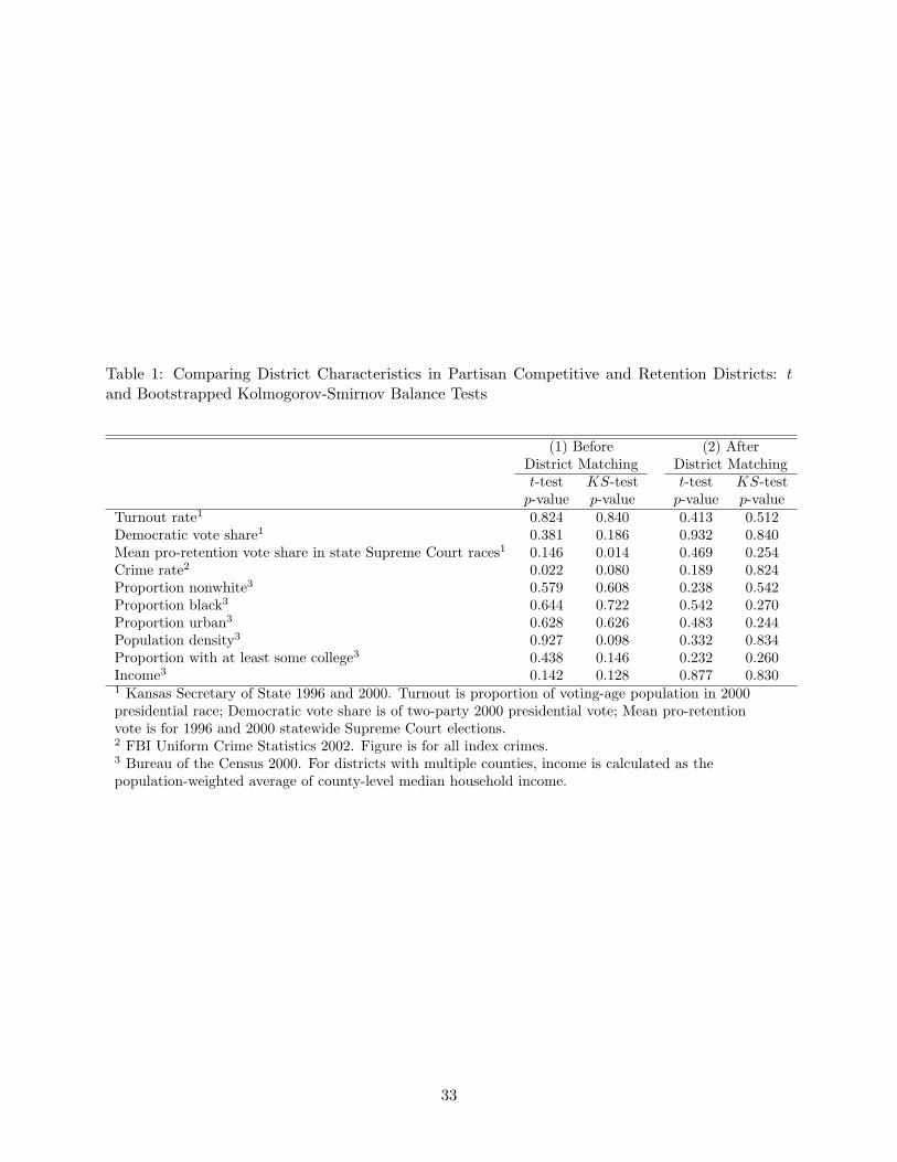
Table 1: Comparing District Characteristics in Partisan Competitive and Retention Districts: tand Bootstrapped Kolmogorov-Smirnov Balance Tests

(1) Before (2) AfterDistrict Matching District Matchingt-test KS-test t-test KS-test

p-value p-value p-value p-valueTurnout rate1 0.824 0.840 0.413 0.512Democratic vote share1 0.381 0.186 0.932 0.840Mean pro-retention vote share in state Supreme Court races1 0.146 0.014 0.469 0.254Crime rate2 0.022 0.080 0.189 0.824Proportion nonwhite3 0.579 0.608 0.238 0.542Proportion black3 0.644 0.722 0.542 0.270Proportion urban3 0.628 0.626 0.483 0.244Population density3 0.927 0.098 0.332 0.834Proportion with at least some college3 0.438 0.146 0.232 0.260Income3 0.142 0.128 0.877 0.8301 Kansas Secretary of State 1996 and 2000. Turnout is proportion of voting-age population in 2000presidential race; Democratic vote share is of two-party 2000 presidential vote; Mean pro-retentionvote is for 1996 and 2000 statewide Supreme Court elections.2 FBI Uniform Crime Statistics 2002. Figure is for all index crimes.3 Bureau of the Census 2000. For districts with multiple counties, income is calculated as thepopulation-weighted average of county-level median household income.

33

Table 2: Summary Statistics for Model Variables

Variable Mean Std. Dev. Min. Max.Ln(1+assigned prison sentence in months) 1.114 1.741 0 8.067

Ln(1+presumptive months prison) 1.017 1.765 0 6.655First guideline regime (1=yes) 0.028 0.164 0 1Second guideline regime (1=yes) 0.422 0.494 0 1Additional counts in conviction 0.462 1.408 0 49Persistent sex offender (1=yes) 0.003 0.057 0 1Firearm used in commission of crime (1=yes) 0.034 0.180 0 1Victim government official (1=yes) 0.019 0.137 0 1Victim child (1=yes) 0.085 0.279 0 1Assault (1=yes) 0.208 0.406 0 1Criminal Threat (1=yes) 0.074 0.262 0 1Robbery (1=yes) 0.080 0.272 0 1Sex Offense (1=yes) 0.108 0.311 0 1Theft (1=yes) 0.235 0.424 0 1Burglary (1=yes) 0.280 0.449 0 1

Appointed counsel (1=yes) 0.784 0.412 0 1Plea bargain (1=yes) 0.940 0.237 0 1Defendant male (1=yes) 0.892 0.310 0 1Defendant nonwhite (1=yes) 0.277 0.448 0 1Defendant Hispanic (1=yes) 0.084 0.277 0 1Defendant age (years) 29.265 10.025 15.439 86.103

District turnout rate 0.534 0.087 0.388 0.803District Democratic vote share 0.401 0.119 0.202 0.671District mean pro-retention vote share 0.753 0.028 0.643 0.822

in state Supreme Court racesDistrict crime rate 24.625 19.232 3.914 73.450District proportion nonwhite 0.167 0.116 0.016 0.418District proportion urban 0.753 0.222 0.134 0.950

Partisan (competitive) district 0.499 0.500 0 1Electoral proximity 0.504 0.257 0 1N=18,141. Sentencing data from Kansas Sentencing Commission. Elections data from KansasSecretary of State. See Table 1 for sources for district demographic data.

34

Table 3: Regression Estimates of the Effect of Judicial Selection Mechanism on Sentencing

All Judges Unchallenged Judges(1) (2) (3) (4) (5) (6)

Ln(1+presumptive months prison) 1.142 1.145 1.152 1.154(0.023) (0.023) (0.024) (0.023)

First guideline regime 0.381 0.339 0.428 0.384(0.169) (0.166) (0.178) (0.175)

Second guideline regime 0.25 0.232 0.23 0.204(0.110) (0.110) (0.118) (0.118)

Additional counts in conviction 0.142 0.148 0.145 0.151(0.020) (0.020) (0.021) (0.022)

Persistent sex offender 1.87 1.891 1.96 1.976(0.405) (0.400) (0.472) (0.466)

Firearm 1.56 1.585 1.596 1.634(0.143) (0.143) (0.159) (0.159)

Victim government official 0.947 0.943 0.86 0.861(0.188) (0.192) (0.204) (0.210)

Victim child -0.107 -0.086 -0.096 -0.08(0.156) (0.159) (0.167) (0.171)

Appointed counsel 0.913 0.879 0.954 0.921(0.077) (0.074) (0.081) (0.079)

Plea bargain -0.98 -1.015 -1.004 -1.028(0.091) (0.093) (0.094) (0.095)

Defendant male 1.302 1.281 1.321 1.3(0.124) (0.122) (0.133) (0.131)

Defendant nonwhite 0.117 0.116 0.113 0.103(0.063) (0.063) (0.065) (0.066)

Defendant Hispanic 0.26 0.148 0.305 0.19(0.107) (0.105) (0.112) (0.107)

Defendant age (years) 0.144 0.145 0.144 0.144(0.016) (0.016) (0.015) (0.015)

Defendant age squared -0.002 -0.002 -0.002 -0.002(0.000) (0.000) (0.000) (0.000)

District turnout rate 1.499 1.644 1.703 1.897(0.692) (0.966) (0.720) (0.963)

District Democratic vote share -0.612 -0.679 -0.863 -0.973(0.828) (0.912) (0.836) (1.006)

District mean pro-retention vote -1.008 -1.461 -1.539 -2.091share in state Supreme Court races (2.305) (2.500) (2.378) (2.589)

District crime rate 0.008 0.008 0.009 0.008(0.003) (0.004) (0.003) (0.004)

District proportion nonwhite 2.941 3.048 3.445 3.645(0.919) (1.185) (1.006) (1.286)

District proportion urban -0.774 -0.626 -0.81 -0.67(0.338) (0.354) (0.320) (0.357)

Partisan (competitive) district 0.268 0.391 0.368 0.268 0.365 0.333(0.108) (0.137) (0.173) (0.104) (0.144) (0.175)

σ 2.624 2.616 2.646 2.637log-likelihood -18067.864 -18036.014 -16315.641 -16282.859

N=18,141 in columns (1) and (2), 16,528 in columns (4) and (5), and 30 in columns (3) and (6).Dependent variable is Ln(1+assigned prison time in months). Standard errors in parentheses.Model specification in columns (1), (2), (4), and (5) is Tobit with groupwise (judge) heteroscedasticity-consistent standard errors. Coefficients for Crime and Year indicators are not reported.Results in columns (3) and (6) are for second-stage weighted-least squares regression described in text.

35

Table 4: Matching Estimates of the Average Effect of Treatment (Potential Competition) on theTreated (Cases in Partisan Competitive Districts)

Fact Pattern District, Then Close District Referenda, ThenMatching Only Fact-Pattern Matching Fact-Pattern Matching

(1) (2) (3) (4) (5) (6)Expected Change in All Judges Unchallenged All Judges Unchallenged All Judges Unchallenged

Pr(prison) 0.036 0.038 0.059 0.056 0.033 0.027(0.006) (0.007) (0.004) (0.005) (0.006) (0.006)

Months prison 0.554 0.551 1.166 1.148 0.439 0.322(unconditional) (0.148) (0.162) (0.068) (0.077) (0.122) (0.130)

Matched observations 4,748 3,890 1,195 1,066 2,491 2,105

Standard errors in parentheses.

36

Table 5: The Effect of Electoral Proximity on Sentencing by Selection Mechanism (Tobit Estimates)(1) (2)

Ln(1+presumptive months prison) 1.145 1.147(0.023) (0.015)

First guideline regime 0.339 0.284(0.165) (0.162)

Second guideline regime 0.228 0.188(0.111) (0.098)

Additional counts in conviction 0.148 0.152(0.020) (0.020)

Persistent sex offender 1.879 1.94(0.398) (0.374)

Firearm 1.581 1.554(0.143) (0.122)

Victim government official 0.940 0.924(0.192) (0.160)

Victim child -0.076 -0.129(0.159) (0.145)

Appointed counsel 0.879 0.904(0.074) (0.071)

Plea bargain -1.015 -0.962(0.092) (0.082)

Defendant male 1.280 1.288(0.122) (0.112)

Defendant nonwhite 0.115 0.085(0.063) (0.060)

Defendant Hispanic 0.146 0.125(0.106) (0.094)

Defendant age (years) 0.145 0.148(0.016) (0.014)

Defendant age squared -0.002 -0.002(0.000) (0.000)

District turnout rate 1.492(0.692)

District Democratic vote share -0.609(0.829)

District mean pro-retention vote -0.988share in state Supreme Court races (2.302)

District crime rate 0.008(0.003)

District proportion nonwhite 2.953(0.919)

District proportion urban -0.777(0.338)

Partisan (competitive) district 0.112(0.185)

Partisan (competitive) district 0.296 0.324× Electoral proximity (0.156) (0.132)

Retention (noncompetitive) district -0.261 -0.270× Electoral proximity (0.174) (0.152)

σ 2.615 2.559log-likelihood -18032.129 -17816.629

N=18,141. Dependent variable is Ln(1+assigned prison time in months). Groupwise (judge) heteroscedasticity-consistent standard errors appear in parentheses. Coefficients for Crime and Year indicators not reportedin both columns. Coefficients for Judge indicators not reported in column (2).

37

Figure 1: Kansas Judicial Districts and Selection Rules

15

8

2

16

25

17

4

24

30

12

20

26

23

6

5

13

9

22

31

11

1

28

14

21

27

19

3

18

7 10

29

Kansas City

Overland Park

Topeka

Wichita

Competitive Partisan District Noncompetitive Retention District

38