Journal of Sound and Vibration (1996) 196(2), 147–164

THE EFFECT OF DECAY RATE VARIABILITY ONSTATISTICAL RESPONSE PREDICTIONS

IN ACOUSTIC SYSTEMS

J. B* R. L. W

Department of Theoretical and Applied Mechanics, Univeristy of Illinois, Urbana, IL 61801,U.S.A.

(Received 15 September 1995, and in final form 14 February 1996)

Statistical predictions for the mean value and variance of both power input and powertransmission in acoustic systems are presented which include the effect of variable modaldecay rates. The newly derived models indicate that the variability of both characteristicsis expected to increase with increasing decay rate variability while predicting the effect.Results from numerical experimentation are presented which confirm both the expectedvariability increase in power transmission and the presented models’ ability to qualitativelyand quantitatively capture the increase.

7 1996 Academic Press Limited

1. INTRODUCTION

In an effort to improve statistical response predictions in reverberation rooms and otherdynamic systems researchers have previously explored the impact of different statisticalmodels for the natural frequency spectrum on response predictions. In a thoroughinvestigation Davy [1] experimentally measured reverberation room transmission functionvariances for comparison with analytical variance predictions based on both a Poissonspectrum model, originally presented by Lyon [2], and a nearest neighbor spectrum modelwhose form was inferred by Davy. Davy found a reasonable agreement between theoryand experiment. The nearest neighbor model provided the best results but stilloverestimated variances when single source and receiver positions were studied. Improvingon both the nearest neighbor and Poisson spectrum models, Weaver [3] proposed that theGaussian orthogonal ensemble (GOE) of random matrix theory [4] provides an accuratemodel for the fluctuations in the natural frequency spectrum of a variety of dynamicsystems [5]. Subsequent application of the GOE spectrum model to reverberation roomtransmission function variances provided an improved statistical estimate predictingreduced variations [6]. While advances in the understanding of spectrum models and theirimpact on response predictions have been made, unexplainable response fluctuations arestill observed.

Unpredictable fluctuations are a particular problem as frequencies of excitation andmodal overlaps decline. It is conjectured here that decay rate fluctuations contribute tothe inaccurate fluctuation predictions at lower frequencies and need to be modeled.Typically the decay rates of the modes contributing to the system’s response are assumedconstant in narrow frequency bands. This is a valid assumption in many systems and is

* Present address. Department of Engineering, Purdue University at Ft. Wayne, 2101 East Coliseum Blvd.,Ft. Wayne, IN 46805-1499, U.S.A.

147

0022–460X/96/370147+18 $18.00/0 7 1996 Academic Press Limited

. . . 148

a widely applied approximation in vibrations and acoustics. Significant variations in decayrates have, however, been observed experimentally at lower frequencies for both theresponse of reverberation rooms [7, 8], and the elastodynamic response of solids [3]. It isthe objective of the current paper to determine the impact of decay rate fluctuations onstatistical response predictions.

Despite renewed interest in improving the statistical models which describe the modalcharacteristics of complex systems, little research has been published concerning thedistribution of decay rates in complex systems. Most of the literature to date concerns thenon-exponential decay of acoustic fields in reverberation chambers [7–9]. An approachmore suitable to a statistical analysis was presented by Schroeder [10] in 1965 whopredicted that the modal decay rates in a complex acoustic field should be distributedaccording to a gamma distribution. More recently the authors have presented a refinedmodel for modal decay rate statistics [11], similar to Schroeder’s, which has been confirmedby numerical experimentation and indicates that modal decay rates are distributedaccording to a chi square distribution. In that study, as in the present, interest centeredon the character of finite difference models of membranes. It was found that the modaldecay rates, b, are distributed according to the probability density function,

p(b)=bB/2−1 e−b(mN/q)

(q/mN)B/2G(B/2), (1)

where N is the total number of nodes in the finite difference model, each with mass m,and B is the number of damped nodes each with viscous damping coefficient q. Extensionof this model to systems of physical interest is straight forward and has been discussedpreviously by Schroeder [10]. More importantly, the above statistical model for thedistribution of decay rates will be used to modify power input and transmission statisticsin acoustic systems.

2. THEORETICAL RESULTS

Statistical estimates for the power input and energy density characteristics of irregularlyshaped, damped membranes are presented in this section. Membranes were chosen for thisstudy because of their relatively easy numerical simulation and their similarity to theacoustic systems which are the primary motivation for this work. Interest is limited tosteady state responses and harmonic excitations where, to date, much of the previousresearch has centered [1, 2, 6]. The methods presented in this chapter for estimating systemcharacteristics are extensions of an approach initiated by Lyon [2] and continued by otherresearchers [1, 6]. The current work, however, is more general than those preceding it andincludes the effect of variable modal decay rates on the statistical predictions. As a result,the work of the previous researchers is encompassed by the current predictions and willbe derived as special cases of the more general results presented here.

The response of linear systems to steady state excitations is conveniently formulated interms of the system’s admittance, T(x� s , x� r ; v), which provides an expression for thesystem’s velocity response to a unit magnitude, harmonic force as a function of sourceposition, x� s , receiver position, x� r , and excitation frequency v. The admittance for anarbitrary, viscously damped membrane of area A and mass density r can be calculateddirectly from the governing equation of motion by exciting the membrane with a unitmagnitude harmonic point force,

92T(x� s , x� r ; v)+ ivz(x� )T(x� s , x� r ; v)+ k2T(x� s , x� r ; v)= ivd(x� − x� s ), (2)

149

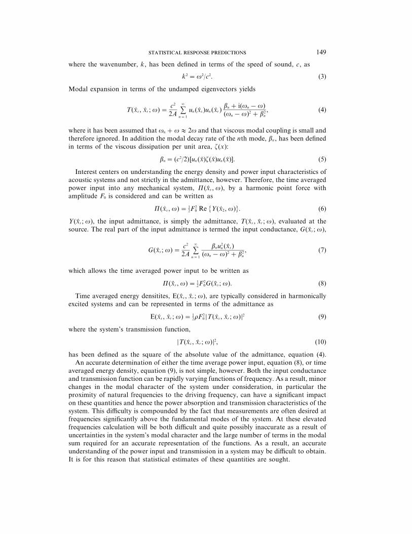
where the wavenumber, k, has been defined in terms of the speed of sound, c, as

k2 =v2/c2. (3)

Modal expansion in terms of the undamped eigenvectors yields

T(x� s , x� r ; v)=c2

2Asa

n=1

un (x� s )un (x� r )bn +i(vn −v)(vn −v)2 + b2

n, (4)

where it has been assumed that vn +v1 2v and that viscous modal coupling is small andtherefore ignored. In addition the modal decay rate of the nth mode, bn , has been definedin terms of the viscous dissipation per unit area, z(x):

bn =(c2/2)[un (x� )z(x� )un (x� )]. (5)

Interest centers on understanding the energy density and power input characteristics ofacoustic systems and not strictly in the admittance, however. Therefore, the time averagedpower input into any mechanical system, P(x� s , v), by a harmonic point force withamplitude F0 is considered and can be written as

P(x� s , v)= 12F

20 Re {Y(x� 2, v)}. (6)

Y(x� s ; v), the input admittance, is simply the admittance, T(x� s , x� r ; v), evaluated at thesource. The real part of the input admittance is termed the input conductance, G(x� s ; v),

G(x� s ; v)=c2

2Asa

n=1

bnu2n (x� s )

(vn −v)2 + b2n, (7)

which allows the time averaged power input to be written as

P(x� s , v)= 12F

20G(x� s ; v). (8)

Time averaged energy densitites, E(x� s , x� r ; v), are typically considered in harmonicallyexcited systems and can be represented in terms of the admittance as

E(x� s , x� r ; v)= 12rF 2

0 =T(x� s , x� r ; v)=2 (9)

where the system’s transmission function,

=T(x� s , x� r ; v)=2, (10)

has been defined as the square of the absolute value of the admittance, equation (4).An accurate determination of either the time average power input, equation (8), or time

averaged energy density, equation (9), is not simple, however. Both the input conductanceand transmission function can be rapidly varying functions of frequency. As a result, minorchanges in the modal character of the system under consideration, in particular theproximity of natural frequencies to the driving frequency, can have a significant impacton these quantities and hence the power absorption and transmission characteristics of thesystem. This difficulty is compounded by the fact that measurements are often desired atfrequencies significantly above the fundamental modes of the system. At these elevatedfrequencies calculation will be both difficult and quite possibly inaccurate as a result ofuncertainties in the system’s modal character and the large number of terms in the modalsum required for an accurate representation of the functions. As a result, an accurateunderstanding of the power input and transmission in a system may be difficult to obtain.It is for this reason that statistical estimates of these quantities are sought.

. . . 150

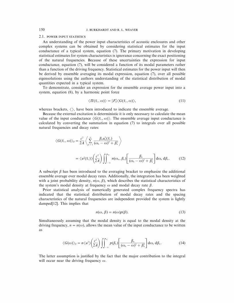
2.1.

An understanding of the power input characteristics of acoustic enclosures and othercomplex systems can be obtained by considering statistical estimates for the inputconductance of a typical system, equation (7). The primary motivation in developingstatistical estimates for system characteristics is ignorance concerning the exact positioningof the natural frequencies. Because of these uncertainties the expression for inputconductance, equation (7), will be considered a function of its modal parameters ratherthan a function of the driving frequency. Statistical estimates for the power input will thenbe derived by ensemble averaging its modal expression, equation (7), over all possibleeigensolutions using the authors understanding of the statistical distribution of modalquantities expected in a typical system.

To demonstrate, consider an expression for the ensemble average power input into asystem, equation (8), by a harmonic point force

�P(x� s , v)�= 12F

20�G(x� s , v)�, (11)

whereas brackets, ��, have been introduced to indicate the ensemble average.Because the external excitation is deterministic it is only necessary to calculate the mean

value of the input conductance �G(x� s , v)�. The ensemble average input conductance iscalculated by converting the summation in equation (7) to integrals over all possiblenatural frequencies and decay rates:

�G(x� s , v)�b =c2

2A W sa

n=1

bnu2n (x� s )

(vn −v)2 + b2n w

= �u2(x� s )�0 c2

2A1 gga

−a

n(vn , bn )$ bn

(vn −v)2 + b2n% dvn dbn . (12)

A subscript b has been introduced to the averaging bracket to emphasize the additionalensemble average over modal decay rates. Additionally, the integration has been weightedwith a joint probability density, n(v, b), which describes the statistical characteristics ofthe system’s modal density at frequency v and modal decay rate b.

Prior statistical analysis of numerically generated complex frequency spectra hasindicated that the statistical distribution of modal decay rates and the spacingcharacteristics of the natural frequencies are independent provided the system is lightlydamped[12]. This implies that

n(v, b)= n(v)p(b). (13)

Simultaneously assuming that the modal density is equal to the modal density at thedriving frequency, n= n(v), allows the mean value of the input conductance to be writtenas

�G(v)�b = n�u2�0 c2

2A1 gga

−a

p(bn )$ bn

(vn −v)2 + b2n% dvn dbn . (14)

The latter assumption is justified by the fact that the major contribution to the integralwill occur near the driving frequency v.

151

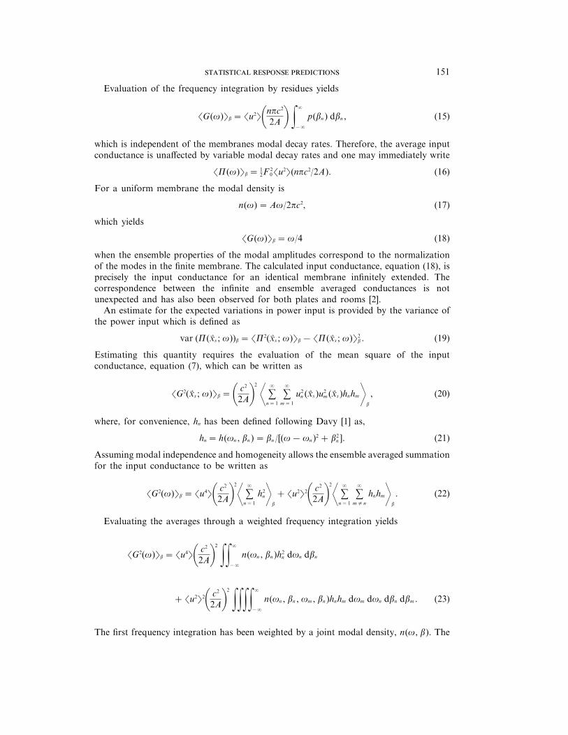
Evaluation of the frequency integration by residues yields

�G(v)�b = �u2�0npc2

2A 1 ga

−a

p(bn ) dbn , (15)

which is independent of the membranes modal decay rates. Therefore, the average inputconductance is unaffected by variable modal decay rates and one may immediately write

�P(v)�b = 12F

20�u2�(npc2/2A). (16)

For a uniform membrane the modal density is

n(v)=Av/2pc2, (17)

which yields

�G(v)�b =v/4 (18)

when the ensemble properties of the modal amplitudes correspond to the normalizationof the modes in the finite membrane. The calculated input conductance, equation (18), isprecisely the input conductance for an identical membrane infinitely extended. Thecorrespondence between the infinite and ensemble averaged conductances is notunexpected and has also been observed for both plates and rooms [2].

An estimate for the expected variations in power input is provided by the variance ofthe power input which is defined as

var (P(x� s ; v))b = �P2(x� s ; v)�b − �P(x� s ; v)�2b . (19)

Estimating this quantity requires the evaluation of the mean square of the inputconductance, equation (7), which can be written as

�G2(x� s ; v)�b =0 c2

2A12

W sa

n=1

sa

m=1

u2n (x� s )u2

m (x� s )hnhmwb

, (20)

where, for convenience, hn has been defined following Davy [1] as,

hn = h(vn , bn )= bn /[(v−vn )2 + b2n ]. (21)

Assuming modal independence and homogeneity allows the ensemble averaged summationfor the input conductance to be written as

�G2(v)�b = �u4�0 c2

2A12

W sa

n=1

h2nwb

+ �u2�20 c2

2A12

W sa

n=1

sa

m$ n

hnhmwb

. (22)

Evaluating the averages through a weighted frequency integration yields

�G2(v)�b = �u4�0 c2

2A12

gga

−a

n(vn , bn )h2n dvn dbn

+ �u2�20 c2

2A12

gggga

−a

n(vn , bn , vm , bn )hnhm dvm dvn dbn dbm . (23)

The first frequency integration has been weighted by a joint modal density, n(v, b). The

. . . 152

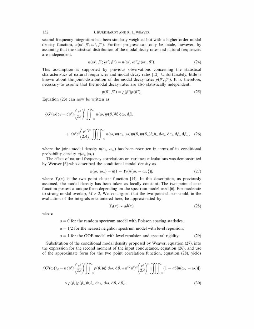
second frequency integration has been similarly weighted but with a higher order modaldensity function, n(v', b', v0, b0). Further progress can only be made, however, byassuming that the statistical distribution of the modal decay rates and natural frequenciesare independent.

n(v', b'; v0, b0)= n(v', v0)p(v', b0). (24)

This assumption is supported by previous observations concerning the statisticalcharacteristics of natural frequencies and modal decay rates [12]. Unfortunately, little isknown about the joint distribution of the modal decay rates p(b', b0). It is, therefore,necessary to assume that the modal decay rates are also statistically independent:

p(b', b0)= p(b')p(b0). (25)

Equation (23) can now be written as

�G2(v)�b = �u4�0 c2

2A12

gga

−a

n(vn )p(bn )h2n dvn dbn

+ �u2�20 c2

2A12

gggga

−a

n(vn )n(vm =vn )p(bn )p(bm )hnhm dvm dvn dbn dbm , (26)

where the joint modal density n(vn , vm ) has been rewritten in terms of its conditionalprobability density n(vm =vn ).

The effect of natural frequency correlations on variance calculations was demonstratedby Weaver [6] who described the conditional modal density as

n(vn =vm )= n[1−Y2(n{vn −vm})], (27)

where Y2(x) is the two point cluster function [14]. In this description, as previouslyassumed, the modal density has been taken as locally constant. The two point clusterfunction possess a unique form depending on the spectrum model used [6]. For moderateto strong modal overlap, Mq 2, Weaver argued that the two point cluster could, in theevaluation of the integrals encountered here, be approximated by

Y2(x)0 ad(x), (28)

where

a=0 for the random spectrum model with Poisson spacing statistics,

a=1/2 for the nearest neighbor spectrum model with level repulsion,

a=1 for the GOE model with level repulsion and spectral rigidity. (29)

Substitution of the conditional modal density proposed by Weaver, equation (27), intothe expression for the second moment of the input conductance, equation (26), and useof the approximate form for the two point correlation function, equation (28), yields

�G2(v)�b = n�u4�0 c2

2A12

gga

−a

p(bn )h2n dvn dbn+n2�u2�20 c2

2A12

gggga

−a

{1− ad[n(vm −vn )]}

×p(bn )p(bm )hnhm dvm dvn dbn dbm . (30)

153

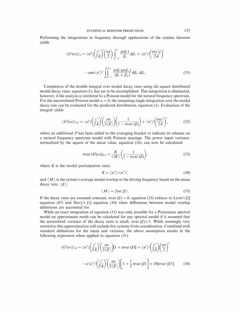
Performing the integrations in frequency through applications of the residue theoremyields

�G2(v)�b = �u4�0 c2

2A12

0np

2 1 ga

−a

p(bn )bn

dbn + �u2�20npc2r

2A 12

−anp�u2�2 gga

−a

p(bn )p(bm )(bn + bm )

dbm dbn . (31)

Completion of the double integral over modal decay rates using chi square distributedmodal decay rates, equation (1), has yet to be accomplished. This integration is eliminated,however, if the analysis is restricted to a Poisson model for the natural frequency spectrum.For the uncorrelated Poisson model a=0, the remaining single integration over the modaldecay rate can be evaluated for the predicted distribution, equation (1). Evaluation of theintegral yields

�G2(v)�b,P = �u4�0 c2

2A12

0 np

2�b�10 11−nvar (b)1+ �u2�20npc2

2A 12

, (32)

where an additional P has been added to the averaging bracket to indicate its reliance ona natural frequency spectrum model with Poisson spacings. The power input variance,normalized by the square of the mean value, equation (16), can now be calculated:

nvar (P(v))b,P =K

�M� 0 11−nvar (b)1, (33)

where K is the modal participation ratio,

K= �u4�/�u2�2, (34)

and �M� is the system’s average modal overlap at the driving frequency based on the meandecay rate, �b�:

�M�=2pn�b�. (35)

If the decay rates are assumed constant, nvar (b)=0, equation (33) reduces to Lyon’s [2]equation (47) and Davy’s [1] equation (10) when differences between modal overlapdefinitions are accounted for.

While an exact integration of equation (31) was only possible for a Poissonian spectralmodel an approximate result can be calculated for any spectral model if it assumed thatthe normalized variance of the decay rates is small, nvar (b)�1. While seemingly veryrestrictive this approximation will exclude few systems from consideration. Combined withstandard definitions for the mean and variance, the above assumption results in thefollowing expression when applied to equation (31):

�G2(v)�db = �u4�0 c2

2A12

0 np

2�b�1[1+nvar (b)]+ �u2�20 c2

2A10np

2 12

−a�u2�20 c2

2A12

0 np

2�b�1$1+12

nvar (b)%+O[nvar (b)2], (36)

. . . 154

where the subscript b has been replaced with db to emphasize that an approximation,nvar (b)�1, has been used. An approximate expression for the normalized variance of theinput power can then be constructed:

nvar (P(v))db =(1/�M�)[(K− a)+ (K− a/2) nvar (b)], (37)

where K and �M� have been defined previously in equations (34) and (35). The expressionindicates that the introduction of a variable modal decay rate, not unexpectedly, causesan increase in the expected power input variance. The percentage increase in the powerinput variance, DPvar , is independent of modal overlap and directly proportional to thenormalized variance of the decay rates:

DPvar =100[1+ (a/2(K− a))] nvar (b).

For constant decay rates, nvar (b)=0, equation (37) reduces to Davy’s [1] equation (10)for a Poissonian spectral model, a=0, and Davy’s equation (12) for the nearest neighborspectrum model, a=1/2.

2.2.

In addition to power input estimates, knowledgable use and analysis of reverberationrooms and other complex systems requires an understanding of mean square energydensities. Statistical estimates for the energy density, equation (9), involves estimating thesystem’s transmission function =T(x� s , x� r ; v)=2.

In a fashion similar to the analyses of both Lyon [2] and Davy [4], the admittance willbe written as

T(x� s , x� r ; v)c2/2A

= sa

n=1

un (x� s )un (x� r )bn −i(vn −v)(vn −v)2 + b2

n= s

a

n=1

usnur

nQn , (38)

where the quantity

Qn =Q(vn , bn )= (bn −i(vn −v))/((vn −v)2 + b2n ) (39)

represents an enhancement factor of the nth mode due to the proximity of the drivingfrequency. The modal amplitudes at the source and receiver position have also been writtenin an abbreviated form: un (x� s )= us

n and un (x� r )= urn . The transmission function can now

be written as

=T(x� s , x� r ; v)=2 =12 0 c2

2A12

sa

n=1

sa

m=1

usnus

murnur

m (QnQ�m +Q�nQm ), (40)

where an overbar has been introduced to indicate that a complex conjugate has been taken.If the statistical character of the frequency spectrum and modal amplitudes are assumedindependent and the modal amplitude statistics are independent in space and for differingmodes, contributions to the sum occur only when n=m. These simplifications allow themean value of the transmission function to be written as

�=T(v)=2�= �u2�20 c2

2A12

W sa

n=1

=Qn =2w. (41)

155

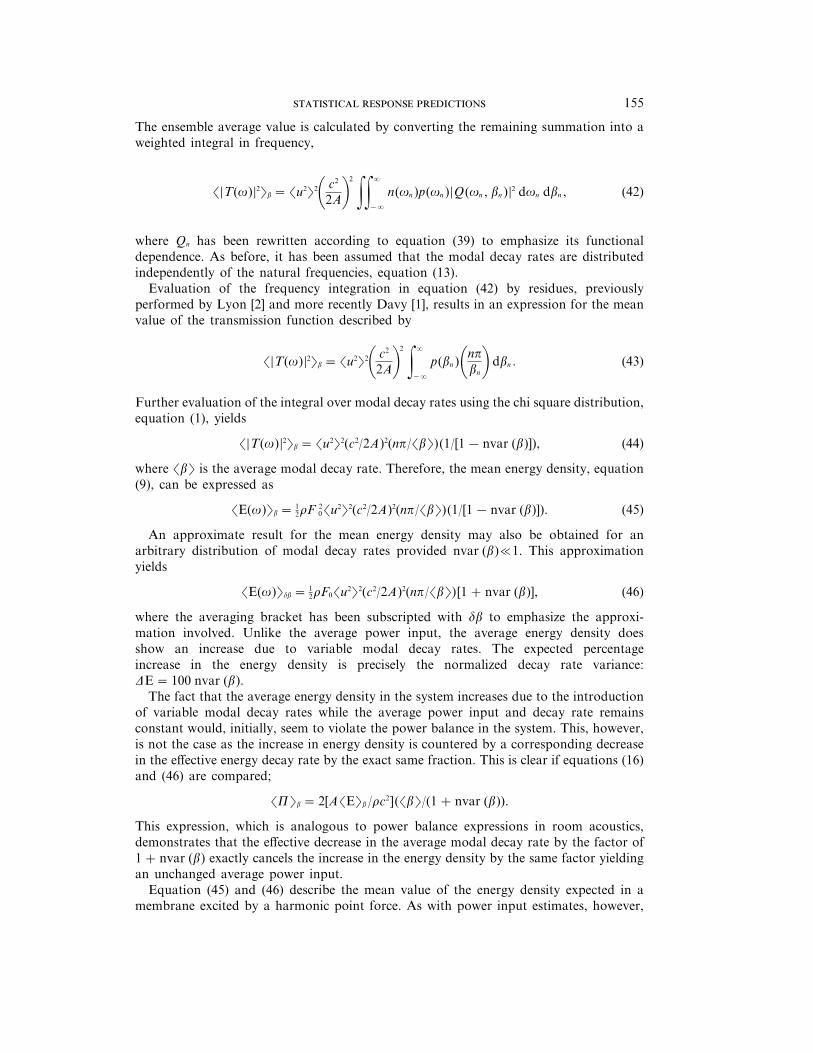
The ensemble average value is calculated by converting the remaining summation into aweighted integral in frequency,

�=T(v)=2�b = �u2�20 c2

2A12

gga

−a

n(vn )p(vn )=Q(vn , bn )=2 dvn dbn , (42)

where Qn has been rewritten according to equation (39) to emphasize its functionaldependence. As before, it has been assumed that the modal decay rates are distributedindependently of the natural frequencies, equation (13).

Evaluation of the frequency integration in equation (42) by residues, previouslyperformed by Lyon [2] and more recently Davy [1], results in an expression for the meanvalue of the transmission function described by

�=T(v)=2�b = �u2�20 c2

2A12

ga

−a

p(bn )0np

bn1 dbn . (43)

Further evaluation of the integral over modal decay rates using the chi square distribution,equation (1), yields

�=T(v)=2�b = �u2�2(c2/2A)2(np/�b�)(1/[1−nvar (b)]), (44)

where �b� is the average modal decay rate. Therefore, the mean energy density, equation(9), can be expressed as

�E(v)�b = 12rF 2

0�u2�2(c2/2A)2(np/�b�)(1/[1−nvar (b)]). (45)

An approximate result for the mean energy density may also be obtained for anarbitrary distribution of modal decay rates provided nvar (b)�1. This approximationyields

�E(v)�db = 12rF0�u2�2(c2/2A)2(np/�b�)[1+nvar (b)], (46)

where the averaging bracket has been subscripted with db to emphasize the approxi-mation involved. Unlike the average power input, the average energy density doesshow an increase due to variable modal decay rates. The expected percentageincrease in the energy density is precisely the normalized decay rate variance:DE=100 nvar (b).

The fact that the average energy density in the system increases due to the introductionof variable modal decay rates while the average power input and decay rate remainsconstant would, initially, seem to violate the power balance in the system. This, however,is not the case as the increase in energy density is countered by a corresponding decreasein the effective energy decay rate by the exact same fraction. This is clear if equations (16)and (46) are compared;

�P�b =2[A�E�b /rc2](�b�/(1+nvar (b)).

This expression, which is analogous to power balance expressions in room acoustics,demonstrates that the effective decrease in the average modal decay rate by the factor of1+nvar (b) exactly cancels the increase in the energy density by the same factor yieldingan unchanged average power input.

Equation (45) and (46) describe the mean value of the energy density expected in amembrane excited by a harmonic point force. As with power input estimates, however,

. . . 156

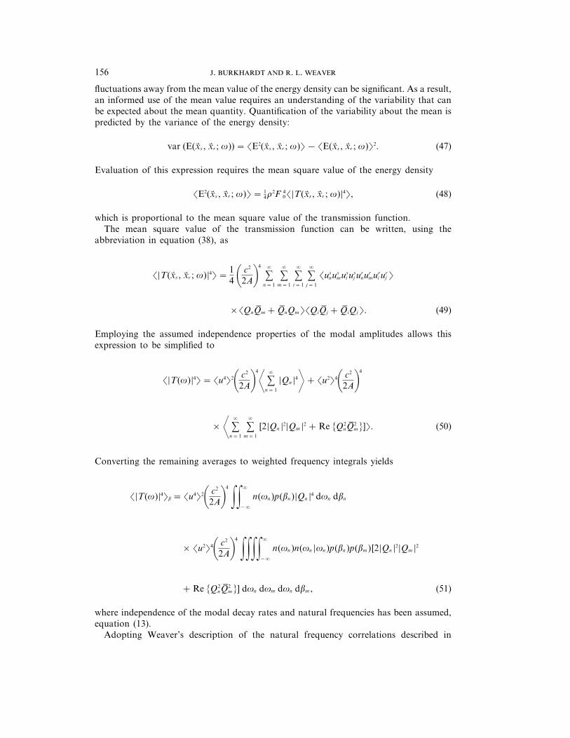
fluctuations away from the mean value of the energy density can be significant. As a result,an informed use of the mean value requires an understanding of the variability that canbe expected about the mean quantity. Quantification of the variability about the mean ispredicted by the variance of the energy density:

var (E(x� s , x� r ; v))= �E2(x� s , x� r ; v)�− �E(x� s , x� r ; v)�2. (47)

Evaluation of this expression requires the mean square value of the energy density

�E2(x� s , x� r ; v)�= 14r

2F 40�=T(x� s , x� r ; v)=4�, (48)

which is proportional to the mean square value of the transmission function.The mean square value of the transmission function can be written, using the

abbreviation in equation (38), as

�=T(x� s , x� r ; v)=4�=14 0 c2

2A14

sa

n=1

sa

m=1

sa

i=1

sa

j=1

�usnus

musi us

j urnur

muri ur

j �

�QnQ�m +Q�nQm��QiQ�j +Q�iQj�. (49)

Employing the assumed independence properties of the modal amplitudes allows thisexpression to be simplified to

�=T(v)=4�= �u4�20 c2

2A14

W sa

n=1

=Qn =4w+ �u2�40 c2

2A14

×W sa

n=1

sa

m=1

[2=Qn =2=Qm =2 +Re {Q2nQ�2

m}]�. (50)

Converting the remaining averages to weighted frequency integrals yields

�=T(v)=4�b = �u4�20 c2

2A14

gga

−a

n(vn )p(bn )=Qn =4 dvn dbn

× �u2�40 c2

2A14

gggga

−a

n(vn )n(vn =vn )p(bn )p(bm )[2=Qn =2=Qm =2

+Re {Q2nQ�2

m}] dvn dvm dvn dbm , (51)

where independence of the modal decay rates and natural frequencies has been assumed,equation (13).

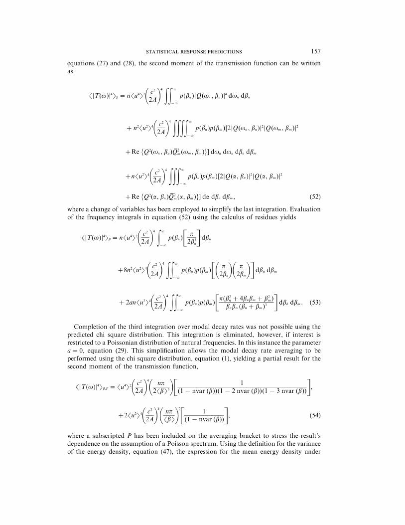
Adopting Weaver’s description of the natural frequency correlations described in

157

equations (27) and (28), the second moment of the transmission function can be writtenas

�=T(v)=4�b = n�u4�20 c2

2A14

gga

−a

p(bn )=Q(vn , bn )=4 dvn dbn

+ n2�u2�40 c2

2A14

gggga

−a

p(bn )p(bm )[2=Q(vn , bn )=2=Q(vm , bm )=2

+Re {Q2(vn , bn )Q�2m (vm , bm )}] dvn dvn dbn dbm

+n�u2�40 c2

2A14

ggga

−a

p(bn )p(bm )[2=Q(a, bn )=2=Q(a, bm )=2

+Re {Q2(a, bn )Q�2m (a, bm )}] da dbn dbm , (52)

where a change of variables has been employed to simplify the last integration. Evaluationof the frequency integrals in equation (52) using the calculus of residues yields

�=T(v)=4�b = n�u4�20 c2

2A14

ga

−a

p(bn )$ p

2b3n% dbn

+8n2�u2�40 c2

2A14

gga

−a

p(bn )p(bm )$0 p

2bn10 p

2bm1% dbn dbm

+2an�u2�40 c2

2A14

gga

−a

p(bn )p(bm )$p(b2n +4bnbm + b2

m )bnbm (bn + bm )3 % dbb dbm . (53)

Completion of the third integration over modal decay rates was not possible using thepredicted chi square distribution. This integration is eliminated, however, if interest isrestricted to a Poissonian distribution of natural frequencies. In this instance the parametera=0, equation (29). This simplification allows the modal decay rate averaging to beperformed using the chi square distribution, equation (1), yielding a partial result for thesecond moment of the transmission function,

�=T(v)=4�b,P = �u4�20 c2

2A14

0 np

2�b�31$ 1(1−nvar (b))(1−2 nvar (b))(1−3 nvar (b))%,

+2�u2�40 c2

2A14

0 np

�b�12

$ 1(1−nvar (b))%, (54)

where a subscripted P has been included on the averaging bracket to stress the result’sdependence on the assumption of a Poisson spectrum. Using the definition for the varianceof the energy density, equation (47), the expression for the mean energy density under

. . . 158

similar assumptions, equation (45), and the definition of the second moment of the energydensity, equation (48), the variance, normalized by its mean value, can be written as

nvar (E(v))b,P =1+K 2

�M� $ 1−nvar (b)(1−2 nvar (b))(1−3 nvar (b))%. (55)

For constant modal decay rates, nvar (b)=0, this result reduces to that previouslypresented by Lyon [2, equation (64)], and Davy [1, equation (5)].

Calculation of a variance prediction for an arbitrary spectrum model and chi squaredistributed modal decay rates has not been possible. However, as in the calculation of themean square value of the admittance, equation (31), an approximate result is possible ifnvar (b)�1. This approximation yields, to leading order in nvar (b),

�=T(v)=4�db = �u4�20 c2

2A14

0 np

2�b�31[1+6 nvar (b)]

+2�u2�40 c2

2A14

0 np

2�b�12

[1+nvar (b)]2

−a�u2�40 c2

2A14

0 np

2�b�31[3+10 nvar (b)], (56)

where db has been used as the subscript for the averaging bracket to indicate theapproximation. An estimate for the variance of the energy density, normalized by thesquare of its mean value, can now be constructed using its definition, equation (47), theexpression for the mean energy density calculated using the same approximation, equation(46), and the definition for the second moment of the energy density, equation (48):

nvar(E(v))db =1+(K 2/�M�)[1+4 nvar (b)]− (a/�M�)[3+4 nvar (b)], (57)

where K and �M� are the participation ratio, equation (34), and the mean modal overlap,equation (35), respectively.

Estimates for the normalized variance of the transmission function with assumedconstant decay rates, similar to those of other researchers [1, 2, 6], can be derived fromthe general expressions (57) by assuming that nvar (b)=0. Substitution yields

nvar (E(v))=1+(K2 −3a)/�M�. (58)

This result corresponds with Weaver’s prediction for the normalized variance [6, equation(11)].

3. NUMERICAL RESULTS

The statistical predictions presented in the last section provide estimates for the dynamiccharacteristics of irregularly shaped membranes and other complex systems excited byharmonic point sources. In particular, expressions were developed describing the variationsthat can be expected in the power input and in the resulting energy densities in the system.The variance predictions describe the variability that can be expected in thesecharacteristics, for example, due to different driving frequencies or for nominally identicalsystems. This generalized ergodicity is thought to apply because changes in the frequencyof excitation, when large in comparison with a typical resonant width, will result in a

159

unique system response dominated by a different collection of natural frequencies. Theaccuracy of these predictions and the applicability of the statistical approach presented hasbeen determined by numerically simulating the response of irregularly shaped membranes.

As with reverberation rooms [1], measurements on the simulated membranes were nottaken at the source position. Therefore, confirmation of the statistical estimates are limtedto a consideration of variances in the membrane’s energy density. The accuracy of theenergy density variance prediction, equation (57), was determined by comparison with theresponse variations observed in numerical simulations of the dynamic response ofirregularly shaped membranes. Since interest has been limited to harmonic point forces,such a comparison could have been performed by simulating the membrane’s steady stateresponse to several harmonic excitations and evaluating the statistical character of theseresults. A more efficient method, however, is to construct transient responses to broadband excitations. Fourier transforms of these responses can then provide information onthe steady state responses of interest. Therefore, statistical information concerning thesystem’s energy density can be obtained by analyzing the square of the magnitude of theFourier transform of the response in frequency.

For the purpose of comparison described above, a finite difference model for a nominallysquare membrane with irregular boundaries was integrated in time. A second ordertemporal central difference scheme was used to construct the solution of the ordinarydifferential equation. The governing differential equation was obtained from a secondorder spatial approximation to the Laplacian, 92, used to generate the membrane’s stiffnessmatrix, [k]. The mass matrix, [m], is the identity matrix while the damping matrix, [c], isalso diagonal but with non-zero entrees corresponding to the damped degrees-of-freedomonly. The meshes considered had a nominal dimension of 199×199 degrees-of-freedomwith a maximum of two sites perpendicularly into the mesh randomly fixed at eachboundary point.

Each mesh considered was impulsively excited at its central node by a Gaussian toneburst 0·05 time units wide at its inflection points with a center frequency of f=40 Hz. Timewas scaled such that all the systems possessed a unit transit time. At the center frequencya wavelength spans approximately seven mesh spacings yielding waves which are nearlyisotropic and non-dispersive. The response of the finite difference equations to thedescribed Gaussian tone burst was integrated in time with a step, dt=0·0025, to ensurestability and a reasonable correspondence between the continuous and discrete model.Each membrane was integrated for a total time corresponding to three hundred transitswith nodal response amplitudes recorded at twenty arbitrarily chosen positions in eachsimulated membrane.

The membrane response at each receiver position, x� ri , was fast Fourier transformed(FFT) yielding the admittance function, Ti (x� s , x� ri ; v), where the receiver position andfrequency response have been subscripted with an i to indicate its reliance on the ithreceiver position. The energy spectra at the individual receiver positions, =Ti (x� s , x� ri ; v)=2,were then calculated from the frequency response function. The power spectra were thennormalized by the power spectral density of the forcing function and adjusted for thefrequency trend in the mean value of the energy density, equation (46), due to an increasingmodal density in frequency, equation (17). The normalized power spectra calculated forthe twenty receiver positions were then combined, resulting in a spatial average overreceiver position, �=Ti (x� s , x� ri ; v)=2�i . The spatially averaged power spectrum was thenstatistically analyzed for it’s variations as a function of frequency producing an estimatefor the normalized variance of the energy density in frequency. All statistics presented inthis study represent spatially averaged frequency statistics; no ensemble averaging wasperformed. Analysis of the power spectrum was limited to a frequency band equal to the

. . . 160

width between the inflection points of the source’s Gaussian power spectrum and centeredat the frequency of the harmonic excitation: 30 Q fQ 50 Hz. Analysis was limited to thisfrequency band to avoid distortions caused by the normalization of the response spectrumdue to small values of the source’s power spectrum at frequencies far from its peak.

The theory presented for variance of the energy density, equation (57), predicts that thenormalized variance of the energy density will increase as a result of a distribution of modaldecay rates. This effect, however, should be undetectable in systems with a narrowdistribution of modal decay rates. For example, in a system with a 1% variation in modaldecay rates the normalized variance can be expected to increase by approximately 4% forthe GOE spectrum model at a modal overlap of one. A 10% enhancement of thenormalized variance of the energy density in a similar system requires approximately a2.5% variation in modal decay rates. Therefore, in the numerical experiments an effort wasmade to choose systems with significant variation in modal decay rates. The expectednormalized variance of modal decay rates is inversely proportional to the number ofdamped sites, B, in the membrane [11]. Using this as an estimate, a 10% increase in thevariance would require about 90 damped sites in the approximately 199×199degree-of-freedom meshes under consideration. Greater enhancement of the energydensities variance would require using fewer damped sites. Using a small number ofdamped sites in the simulation, however, requires extremely larger damper strengths toachieve significant modal overlaps. With 90 damped sites a damper strength ofapproximately twenty, c=20, would be required to achieve a modal overlap of 10 in thesystems under investigation. Such a large damper strength is physically unrealistic. At theseelevated damper strenghts it is possible that such a site would appear blocked rather thandamped. Therefore, achieving substantial modal decay rate variances and significant modaloverlap is not straightforward.

To simulate systems with few damped sites, and hence significant variances in modaldecay rates, the viscous dampers were grouped into pods approximately one half of awavelength across. This allows groups of several damped sites to appear as one dampedsite to the system. This approach allows the effective number of damped sites in themembrane, Be , to be reduced, resulting in an increased decay rate variance. Thecorrespondence between the number of damped sites, B, and the number of pods, however,is only approximate. Uncertainty regarding the modal decay rate variance and the propervalue for the number of equivalent damped sites, Be , in the simulated systems demandedthat this parameter be determined from the response of the membrane. This parameter canbe determined from the temporal decay of the membrane’s response. Response decays aretypically considered to be exponential in time. Such exponential behavior follows only ifthe individual modes which compose the response possess identical decay rates. Whenmultiple decay rates are present in a system, however, the diffuse field decays in anonexponential manner. The form of the temporal decay of the spatially average, squareamplitude, d(t), can be determined by averaging the exponential decay of the constituentmodes using the known distribution for the modal decay rates, equation (1),

d(t)=ga

−a

p(b) e−2bt db. (59)

Evaluation of this integral yields an expression for the decay of the spatially averagedsquare amplitude of the form

d(t)= [1+ (2 var (b)/�b�)t]−1/nvar(b), (60)

similar to that originally described by Schroeder [10]. Spatially averaged decays from the

161

simulated membranes were fitted to this expression by employing a non-linear least squarefit which provided an immediate estimate for the average decay rate, �b�, and itsnormalized variance nvar (b). A similar procedure could be used to determine the decayrate variances in experimental systems. In this work the non-linear square curve fit wasperformed using the subroutine package MINPACK.

Energy density statistics were generated by numerical simulation for a series ofmembranes with varying modal overlap and a variety of damper distributions. Forcomparative purposes a series of membranes with a small modal decay rate variance wasinvestigated for comparison with the previous predictions for energy density statisticswhich neglect the effect of varying modal decay rates [1, 2]. The membranes considered had20% of their sites viscously damped at randomly distributed sites throughout the mesh. Allthe systems simulated in this study were substantially reverberant. The energy decay pertransit time ranged from 0·004 at a modal overlap of one to 0·050 at a modal overlap ofapproximately thirteen. Therefore, the most lightly damped system allowed 250 transitsbefore the amplitude of the transient decreased by a factor of e. The most heavily dampedmembranes allowed 20 such transits. A curve fit of the reverberant decay determined thenormalized variance of the modal decay rates involved in the response, nvar (b)=0·001.

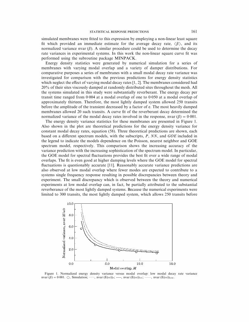
The energy density variance statistics for these membranes are presented in Figure 1.Also shown in the plot are theoretical predictions for the energy density variance forconstant modal decay rates, equation (58). Three theoretical predictions are shown, eachbased on a different spectrum models, with the subscripts, P, NN, and GOE included inthe legend to indicate the models dependence on the Poisson, nearest neighbor and GOEspectrum model, respectively. This comparison shows the increasing accuracy of thevariance prediction with the increasing sophistication of the spectrum model. In particular,the GOE model for spectral fluctuations provides the best fit over a wide range of modaloverlaps. The fit is even good at higher damping levels where the GOE model for spectralfluctuations is questionably accurate [11]. Reasonably accurate variance predictions arealso observed at low modal overlap where fewer modes are expected to contribute to asystems single frequency response resulting in possible discrepancies between theory andexperiment. The small discrepancy which is observed between the theory and numericalexperiments at low modal overlap can, in fact, be partially attributed to the substantialreverberance of the most lightly damped systems. Because the numerical experiments werelimited to 300 transits, the most lightly damped system, which allows 250 transits before

Figure 1. Normalized energy density variance versus modal overlap: low modal decay rate variancenvar (b)=0·001. w, Simulation; ·····, nvar (E(v))P ; ----, nvar (E(v))NN ; ——, nvar (E(v))GOE .

. . . 162

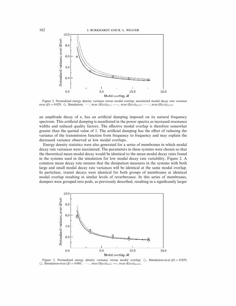
Figure 2. Normalized energy density variance versus modal overlap: maximized modal decay rate variancenvar (b)=0·029. e, Simulation; ·····, nvar (E(v))db,P ; -----, nvar (E(v))db,NN ; ——, nvar (E(v))db,GOE .

an amplitude decay of e, has an artificial damping imposed on its natural frequencyspectrum. This artificial damping is manifested in the power spectra as increased resonancewidths and reduced quality factors. The effective modal overlap is therefore somewhatgreater than the quoted value of 1. The artificial damping has the effect of reducing thevariance of the transmission function from frequency to frequency and may explain thedecreased variance observed at low modal overlaps.

Energy density statistics were also generated for a series of membranes in which modaldecay rate variances were maximized. The parameters in these systems were chosen so thatthe theoretical mean modal decay would be identical to the mean modal decay rates foundin the systems used in the simulation for low modal decay rate variability, Figure 2. Acommon mean decay rate ensures that the dissipation measures in the systems with bothlarge and small modal decay rate variances will be identical at the same modal overlap.In particluar, transit decays were identical for both groups of membranes at identicalmodal overlap resulting in similar levels of reverberance. In this series of membranes,dampers were grouped into pods, as previously described, resulting in a significantly larger

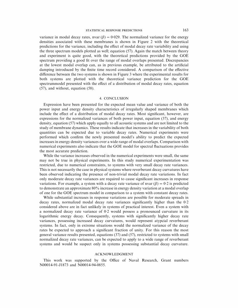
Figure 3. Normalized energy density variance versus modal overlap: r, Simulation-nvar (b)=0·029;w, Simulation-nvar (b)=0·001; ——, nvar (E(v))GOE ; ----, nvar (E(v))db,GOE .

163

variance in modal decay rates, nvar (b)=0·029. The normalized variance for the energydensities associated with these membranes is shown in Figure 2 with the theoreticalpredictions for the variance, including the effect of modal decay rate variability and usingthe three spectrum models plotted as well; equation (57). Again the match between theoryand experiment is quite good, with the theoretical predictions provided by the GOEspectrum providing a good fit over the range of modal overlaps presented. Discrepanciesat the lowest modal overlap can, as in previous example, be attributed to the artificialdamping introduced by the finite time record considered. A comparison of the effectivedifference between the two systems is shown in Figure 3 where the experimental results forboth systems are plotted with the theoretical variance prediction for the GOEspectrummodel presented with the effect of a distribution of modal decay rates, equation(57), and without, equation (58).

4. CONCLUSION

Expression have been presented for the expected mean value and variance of both thepower input and energy density characteristics of irregularly shaped membranes whichinclude the effect of a distribution of modal decay rates. Most significant, however, areexpressions for the normalized variances of both power input, equation (37), and energydensity, equation (57) which apply equally to all acoustic systems and are not limited to thestudy of membrane dynamics. These results indicate that increases in the variability of bothquantities can be expected due to variable decay rates. Numerical experiments wereperformed which confirm the newly presented model’s ability to predict the expectedincreases in energy density variances over a wide range of modal overlaps. Comparison withnumerical experiments also indicate that the GOE model for spectral fluctuations providesthe most accurate prediction.

While the variance increases observed in the numerical experiments were small, the samemay not be true in physical experiments. In this study numerical experimentation wasrestricted, due to numerical constraints, to systems with very small decay rate variances.This is not necessarily the case in physical systems where reverberant decay curvatures havebeen observed indicating the presence of non-trivial modal decay rate variations. In factonly moderate decay rate variances are required to cause significant increases in responsevariations. For example, a system with a decay rate variance of nvar (b)=0·2 is predictedto demonstrate an approximate 80% increase in energy density variation at a modal overlapof one for the GOE spectrum model in comparison to a system with constant decay rates.

While substantial increases in response variations are possible for moderate spreads indecay rates, normalized modal decay rate variances significantly higher than the 0·2considered above are in fact unlikely in systems of practical interest. Even a system witha normalized decay rate variance of 0·2 would possess a pronounced curvature in itslogarithmic energy decay. Consequently, systems with significantly higher decay ratevariances, possessing increased decay curvatures, would represent atypcial reverberantsystems. In fact, only in extreme situations would the normalized variance of the decayrates be expected to approach a significant fraction of unity. For this reason the mostgeneral variance results presented, equations (37) and (57), restricted to systems with smallnormalized decay rate variances, can be expected to apply to a wide range of reverberantsystems and would be suspect only in systems possessing substantial decay curvature.

ACKNOWLEDGMENT

This work was supported by the Office of Naval Research, Grant numbersN00014-91-J1873 and N00014-94-0855.

. . . 164

REFERENCES

1. J. L. D 1981 Journal of Sound and Vibration 77, 455–479. The relative variance of thetransmission function of a reverberation room.

2. R. H. L 1969 Journal of the Acoustical Socity of America 45, 545–565. Statistical analysisof power injection and response in structures and rooms.

3. R. L. W 1989 Journal of the Acoustical Society of America 85, 1005–1013. Spectral statisticsin elastodynamics.

4. O. B, M.-J. G and C. S 1986 in Quantum Chaos and Statistical NuclearPhysics, 18–40. New York: Springer. Spectral fluctuations of classically chaotic system.

5. O. L, C. S and D. S 1992 Europhysics Letters 18, 101–106. Quantum chaosmethods applied to high-frequency plate vibrations.

6. R. L. W 1989 Journal of Sound and Vibration 130, 487–491. On the ensemble variance ofreverberation room transmission fucntions. The effect of spectral rigidity.

7. K. B 1980 Journal of Sound and Vibration 73, 19–29. Monotonic curvature of lowfrequency decay records in reverberation chambers.

8. F. K and K. Y 1986 Journal of the Acoustical Society of America 80, 543–554.A systematic study of power-law decays in reverberation rooms.

9. T. B and S. L. Y 1982 Journal of the Acoustical Society of America 72, 1838–1844.Curvature of sound decays in partially reverberant rooms.

10. M. R. S 1965 in 5th International Congress on Acoustics, Liege G31, 1–4. Some newresults in reverberation theory.

11. J B and R. L. W 1996 Journal of the Acoustical Society of America 100,in press. Spectral statistics in damped systems—Part I. Modal decay rate statistics.

12. J B 1995 Ph.D Thesis, University of Illinois, Statistical response predictions indamped, complex systems.

13. J B and R. L. W 1996 Journal of the Acoustical Society of America 100,in press. Spectral statistics in damped systems—Part II. Spectral denisty fluctuations.

14. T. A. B, J. F, J. B. F, P. A. M, A. P and S. S. W 1986 Reviewsof Modern Physics 53, 385–479. Random matrix physics: spectrum and strength fluctuations.