The Effect of Cultural and Political Factors on FDI B. 325537 - id...1 The Effect of Cultural and Political Factors on FDI Between the US and Partner Countries Author: B.F.M. Lausberg

1

The Effect of Cultural and Political Factors on FDI

Between the US and Partner Countries

Author: B.F.M. Lausberg

EUR study number: 325537

Thesis supervisor: Prof. J.M. Viaene

Finish date: [month year]

ERASMUS UNIVERSITY ROTTERDAM

ERASMUS SCHOOL OF ECONOMICS

MSc Economics & Business

Master Specialization Financial Economics

2

PREFACE AND ACKNOWLEDGEMENTS

NON-PLAGIARISM STATEMENT

By submitting this thesis the author declares to have written this thesis completely by himself/herself, and not to

have used sources or resources other than the ones mentioned. All sources used, quotes and citations that were

literally taken from publications, or that were in close accordance with the meaning of those publications, are

indicated as such.

COPYRIGHT STATEMENT

The author has copyright of this thesis, but also acknowledges the intellectual copyright of contributions made by

the thesis supervisor, which may include important research ideas and data. Author and thesis supervisor will have

made clear agreements about issues such as confidentiality.

Electronic versions of the thesis are in principle available for inclusion in any EUR thesis database and repository,

such as the Master Thesis Repository of the Erasmus University Rotterdam

3

ABSTRACT

Foreign direct investment is a major form of international capital transfer and has increased

substantially over the last decades as a consequence of rising global economic integration. It

has even grown faster than world GDP and merchandise trade even despite of the large drop

in world FDI flows at the turn of the millennium. The two-way flow between developed

countries still accounts for the largest part of asset trade. Around 80% of total FDI flows are

invested between developed countries. Furthermore, inward FDI stock of developing

countries has decreased over the last eight years as a percentage of total inward FDI stock. If

developing countries want to reverse this trend it is important for governments and

companies of these developing countries to know which factors determine bilateral FDI

stock. This paper has tried to contribute empirical findings and results to the question as to

what way cultural and political factors influence asset trade and in particular FDI. Therefore,

this paper investigated a set of bilateral US inward and outward FDI stock data for the time

period 1985-2006 in a panel with 37 countries. Cultural differences proved to have a

significant negative effect on bilateral FDI stock. Also, the results demonstrated a significant

effect of the type of legal family in a country on FDI. However, the effect of belonging to

same legal family is negative. The political situation in a country proved to be a significant

determinant of bilateral FDI stock. Countries with a low political rank receive more FDI from

the US.

4

TABLE OF CONTENTS PREFACE AND ACKNOWLEDGEMENTS ........................................................................... 2

ABSTRACT ............................................................................................................................... 3

LIST OF TABLES ..................................................................................................................... 5

1. INTRODUCTION ............................................................................................................. 6

2. THEORY ......................................................................................................................... 10

2.1 FDI flows depend on international informational asymmetries ................................ 10

2.2 The link between informational asymmetry and distance; the gravity model .......... 12

2.3 The link between informational asymmetry and cultural and political Differ. ......... 14

2.4 Political instability causes risk .................................................................................. 17

2.5 Hypotheses ................................................................................................................ 18

3. METHODOLOGY .......................................................................................................... 21

3.1 Variables explained ................................................................................................... 21

3.2 Model ........................................................................................................................ 26

3.3 Gravity equations ...................................................................................................... 30

3.3.1 Basic gravity equation........................................................................................ 30

3.3.2 Augmented gravity equation .............................................................................. 31

3.3.3 Augmented gravity equation including explaining variables separately ........... 31

3.3.4 Total gravity equation including all explaining variables .................................. 31

3.3.5 Time and country fixed effects model ............................................................... 32

4. RESULTS ........................................................................................................................ 33

4.1 Results ....................................................................................................................... 33

4.1.1 Basic gravity model ........................................................................................... 33

4.1.2 Augmented gravity model.................................................................................. 34

4.1.3 Augmented gravity model including explaining variables separately ............... 35

4.1.4 Total model including all explaining variables .................................................. 37

4.1.5 Time and country fixed effects models .............................................................. 41

4.1.6 Comparing the parameters for different models ................................................ 46

4.1.7 Wald-test ............................................................................................................ 52

4.1.8 Robustness check ............................................................................................... 53

4.2 Discussion ................................................................................................................. 54

5. CONCLUSION ................................................................................................................ 59

REFERENCES ........................................................................................................................ 61

APPENDICES ......................................................................................................................... 61

5

LIST OF TABLES

Table 1.1: FDI Stock Developed & Developing Countries 6

Table 4.1: Basic Gravity Model 33

Table 4.2: Augmented Gravity Model 34

Table 4.3: Total Gravity Model: incl. Legal Family and Political Difference indicators 38

Table 4.4: Total Gravity Model: incl. Legal Family 01 and Political Difference indicators 38

Table 4.5: Total Gravity Model: incl. Legal Family and Political Rank indicators 39

Table 4.6: Total Gravity Model: incl. Legal Family 01 and Political Rank indicators 39

Table 4.7: Total Gravity Model: incl. Legal Family and Political Difference indicators (Time Fixed) 42

Table 4.8: Total Gravity Model: incl. Legal Family 01 and Political Difference indicators (Time Fixed) 42

Table 4.9: Total Gravity Model: incl. Legal Family and Political Difference indicators (Time Fixed) 43

Table 4.10: Total Gravity Model: incl. Legal Family 01 and Political Rank indicators (Time Fixed) 43

Table 4.11: Augmented Gravity Model (Country Fixed) 45

Table 4.12: Parameters & probabilities of Legal Family & Legal Family 01 46

Table 4.13: Parameters & probabilities of Culture 46

Table 4.14: Parameters & probabilities of Voice and Accountability indicator 47

Table 4.15: Parameters & probabilities of Political Stability No Violence indicator 48

Table 4.16: Parameters & probabilities of Government effectiveness indicator 49

Table 4.17: Parameters & probabilities of Regulatory Quality indicator 49

Table 4.18: Parameters & probabilities of Rule of Law indicator 50

Table 4.19: Parameters & probabilities of Control of Corruption indicator 51

Table 4.20: Wald-Test 52

Table 4.21: Robustness Check 53

Appendix

Table 1: Differences in Hofstede's cultural indicators between the US and partner countries 65

Table 2: Rank of Political indicators 66

Table 3: FDI stock between the US and trading partners 66

Table 4: Total FDI Stock Basic Gravity Model; including Explaining Variables Separately 67

Table 5: Inward FDI Stock Basic Gravity Model; including Explaining Variables Separately 68

Table 6: Outward FDI Stock Basic Gravity Model; including Explaining Variables Separately 69

6

1. INTRODUCTION




in world FDI flows at the turn of the millennium. Over the last 15 years, before the beginning

of the crisis, FDI had increased by over 400%. Forces that drive global economic integration

true FDI are initiated by prospects of reduced risk true diversification of investment

opportunities, reduced costs of capital for businesses and better allocation of capital. All these

forces must ultimately lead to increased economic growth (Guerin, 2006).

Large multinational enterprises are the main drivers of this emerging global economy, while

they internationalize their production chains and expand internationally by entering new

markets to reach more consumers. Currently one-third of world trade is accounted for by

MNE‟s, which is for the largest part intra-firm trade. FDI‟s most important feature is that it is

prominent in industries where the classical competitive paradigm is the most ill fitting

(Brouwer et al, 2008). The two-way flow between developed countries still accounts for the

largest part of asset trade. Around 80% of total FDI flows are invested between developed

countries. Furthermore, inward FDI stock of developing countries has decreased over the last

eight years as a percentage of total inward FDI stock.

Table 1.1: FDI Stock Developed & Developing Countries

Inward FDI Stock 1990 2000 2008 Outward FDI Stock 1990 2000 2008

Developed Countries 1.412.605 3.960.321 10.212.893 Developed Countries 1.640.405 5.186.178 13.623.626Developing Countries 529.593 1.736.167 4.275.982 Developing Countries 145.179 862.358 2.356.649

Developing Countries as Developing Countries asPercentage of Total 27,3% 30,5% 29,5% Percentage of Total 8,1% 14,3% 14,7%

This development is unfavourable for developing countries, as Foreign Direct Investments

are regarded as a substantial contributor to international economic integration and

development in general. According to Borensztein et al. (1998) Foreign Direct Investments

contribute more to growth than domestic investments. In addition, FDI flows are also more

advantageous and sustainable than other international asset flows, because of the intent of

foreign direct investors to enter into a long-term relationship. Moreover, Brenton et al.

(1999) conclude in their article that FDI induces managerial and technological knowledge

7

spill-overs, which lead to expanded export opportunities, increased international linkages,

and more domestic competition and consequently increased product variety.

“OECD recommends that a direct investment enterprise be defined as an incorporated or

unincorporated enterprise in which a foreign investor owns 10 per cent or more of the

ordinary shares or voting power of an incorporated enterprise or the equivalent of an

unincorporated enterprise. Foreign Direct Investment is a cross-border investment made by

an investor with the intent of obtaining a long-lasting interest in an enterprise resident in

another country” (OECD). Basically, a firm can employ a variety of methods when it wishes

to make sales abroad. A firm can export its products, it can license a foreign company,

appoint agents or can engage in Foreign Direct Investment. By engaging in Foreign Direct

Investment it is possible for a firm to produce directly in the country it wishes to sell its

products (Petroulas, 2006).

FDI exists in several major forms. The first type is called horizontal FDI, which is market

oriented and gives companies access to foreign markets. In this form FDI is acting as a

substitute for trade. The second is called vertical FDI, which is production oriented and

enables transnational organizations to minimize their costs. These global companies try to

gain strategic advantage by shifting low-paid jobs abroad while keeping high value added

research at home. By applying this strategy TNOs produce either parts of or the entire final

product in low-cost countries. In this form FDI is acting as a complement for trade. FDI

flows are often seen as either a substitute for trade (horizontal FDI) or as a complement to

trade (vertical FDI). A third type of rationale implies that the mode of outsourcing depends

on the market structure, while companies in oligopolistic markets make extra profits,

companies in competitive markets can lower their costs. A theoretical explanation of the

difference between horizontal and vertical FDI is that firms engaging in horizontal FDI are

said to sell their products in foreign markets, unlike firms that engage in vertical FDI which

are said to serve the home market (Guerin, 2006).

Besides increasing FDI flows there exists another important feature of global economic

integration. The role of cultural and political differences, which is often seen as an interfering

factor in realizing global economic integration, has been the subject of many scientific

articles (Shenkar, 2001). According to Shenkar (2001) “cultural distance” is a widely used

8

construct in international business where it has been applied to, amongst others, foreign

investment expansion, entry mode choice, and the performance of foreign invested affiliates.

In the middle of the last century Tinbergen (1962) and Pöyhönen(1963) conducted research

on bilateral trade and foreign investment and independently introduced a gravity equation

framework used in empirical analyses. Since then researchers have applied the gravity

equation framework extensively and successfully to a large number of policy issues. They

have applied it, for example, to study the effect of exchange rates, a common currency, trade

policies or regional integration.

Most recently, the scope of the gravity equation framework has been expanded by researchers

who introduced variables that represent political and cultural differences to the gravity model.

Their aim is to identify the effect of cultural and political factors on asset trade (Flörkemeier,

2002; Guiso et al., 2009; Kalemli-Ozcan and Sorensen, 2007; Heuchemer and Sander, 2007;

Heuchemer et al., 2008). These studies present empirical results which show that trust in

other countries, institutions, trust in these institutions, and cultural differences are important

drivers, or on the contrary important barriers, to economic exchange. Heuchemer et al. (2008)

investigate the determinants of European banking market integration with a focus on these

cultural and political differences. They employ a dataset of European cross-border loans and

deposits and use various gravity models that are augmented by societal proxies. These

societal proxies consist of variables that measure the Euclidean distance of different cultural

and political factors between European countries.

To our knowledge these societal proxies have not yet been used to investigate FDI stock

between US and partner countries. This thesis will try to contribute empirical findings and

results to the question as to what way cultural and political factors influence asset trade and in

particular FDI. In this study I will first test the gravity equation and secondly, the societal

proxies, the indicators of differences in culture and political situation to measure the effect of

cultural and political factors on FDI stock between the US and their trading partner countries.

I will use a set of bilateral US inward and outward FDI stock data for the time period 1985-

2006 in a panel with 37 countries. My objective is to answer three questions:

9

Do cultural differences affect the amount of FDI stock between the US and a trading partner

and to what extent is there any difference between the amount of inward and outward stock?

Do political differences affect the amount of FDI stock between the US and a trading partner

and to what extent is there any difference between the amount of inward and outward stock?

Does the quality of the political situation in a partner country affect the amount of FDI stock

between the US and a trading partner and to what extent is there any difference between the

amount of inward and outward stock?

This study could have implications on both theory and policy. If cultural and political

variables can explain the patterns of bilateral FDI stock a country‟s financial integration

depends on it. By taking the US as example we could be able to explain which part of FDI

stock does not depend on easily changeable policy, like exchange rates or tax rates, but on

robust factors like culture and political situation. As we have seen above total outward FDI

stock towards developing countries has decreased during the last eight years. Our results

could be helpful for governments in developing countries to adapt their policy for attracting

FDI.

Before those results can be presented, section 2 will first present the theoretical background,

including theory on informational asymmetries, the gravity model, and political and cultural

differences. It also defines the hypotheses tested in this thesis. Section 3 discusses the

methodology of the empirical research, including an explanation of the variables, the model,

and the gravity equations that are being used. In section 4, the empirical results will be

presented alongside the different gravity equations that are being used. This will be

completed by a robustness check and a Wald-test, followed by a discussion of the results. The

thesis will be concluded in section 5.

10

2. THEORY

This chapter will discuss different theories that could explain the influence of political and

cultural factors on FDI. Besides Empirical FDI research different articles are mentioned

whose subjects are information asymmetry and investment risk caused by political instability.

Subsequently, we will try to derive hypotheses out of this theoretical background.

2.1 FDI flows depend on international informational

asymmetries

Consistent with portfolio diversification theory and the neoclassical model, equity flows

should be geographically dispersed to maximize the overall yield. However, it is a stylized

fact that FDI flows are geographically concentrated in certain regions and countries.

Prospects of more efficient allocation of capital, diversification of investment opportunities,

reduced cost of capital for businesses and economic growth drive the forces of financial

integration, as they drive the forces of global economic integration. Nevertheless, in

international financial markets the problems of information asymmetry are well recognized.

Different articles mention the biased foreign asset portfolios of countries towards the

domestic market. These biased portfolios are not optimally diversified and cause market

frictions (French and Poterba, 1991; Tesar and Werner, 1995).

Lane (2001) accentuates that despite the highly increased pace of globalization, behavioural

and informational barriers keep restricting the integration of the global capital market.

Furthermore, Portes et al. (2001) and Portes and Rey (2000) investigate bilateral equity flows

and bonds in a panel data regression model based on a gravity equation. In their sample the

information effect dominates the diversification effect. They state that there is only weak

support for a diversification motive. Just when they control for informational frictions they

find little proof of a diversification motive. In discussions of capital mobility and

globalization it is often assumed that international capital markets are frictionless but this

seems not to be the case, when looking at informational barriers.

Informational asymmetries appear to be the main cause of capital market segmentation.

Theories on asset trade are mainly dominated by models based on autarky prices, factor

11

endowments and comparative advantage. (Helpman and Razin, 1978; Svensson, 1988;

Obstfeld and Rogoff, 1996), while those theories should be dominated by models based on

differentiated assets, transaction costs, information asymmetries, and some kind of familiarity

effect (Heath and Tversky, 1991; Huberman, 2001). A shift should be made towards these

models like the shift in goods trade on theoretical modeling. In finance, literature information

asymmetries are more frequently used than in asset trade literature, although it emphasizes on

portfolio choice and asset pricing rather than on transaction volumes.

There are, however important factors to learn from finance literature. Gordon and Bovenberg

(1996) have developed a model at a macro level between foreign and domestic investors. In

their paper they concluded that there was an indirect but substantial support for the

informational asymmetry hypothesis. Their paper was based on a relationship between

current account deficits and real interest rates. Portes et al. (2001) use a sample in their paper,

which is strictly US centered, in which they find that an assets required level of information

determines the importance of the information variables. For example, assets with high

information content, such as corporate bonds, are explained for a greater part by information

variables rather than assets with low information content like treasury bonds. According to

this theory, information variables should be important explanatory variables for the prediction

of FDI flows, because of their high information content.

Ahearne et al. (2004) investigate in their paper the importance of a public listing in the US

for foreign firms. They conclude that a public listing is an important way to reduce

information costs, since public listings are standardized and produce credible financial

information. Their results demonstrate that a country‟s total amount of US publicly listed

companies explained for a substantial part a country‟s weight in US investors‟ portfolio.

Foreign countries in which companies do not commit to the US regulatory environment are

presented for a smaller part in US equity portfolios. This is an important factor behind the

home bias phenomenon.

Huberman (2001) researched a sample of shareholders of Regional Bell Operating

Companies and his results show that when people invest abroad they often invest in the

familiar and by doing that ignore the principals of portfolio theory. So they do not base their

12

investments purely on diversification principles but one some kind of “familiarity”. French

and Poterba (1991) also appeal to information asymmetry or some type of „familiarity‟ effect.

Transaction costs increase with information asymmetry, which reduces international bilateral

equity flows. Information asymmetry is directly influenced by a familiarity effect and this

familiarity effect declines with economic distance. Economic distance depends mainly on two

factors. Firstly, economic distance depends on national and governmental differences, which

are explained by differences and dissimilarities of institutions, political situation and culture.

This is also the main subject and research question of this paper. Secondly, economic

distance depends on geographical distance, which is attended to in the next section.

2.2 The link between informational asymmetry and distance; the

gravity model

Tesar (1995) studies the portfolio choices of Canadian and US investors and concludes in his

article that, to the extent that investors do invest in foreign securities, investors‟ decisions are

not purely made based on diversification motives. Alternatively, geographical distance seems

to be an important factor in the explanation of international portfolio investment decision.

Coval (1999) states that investors have easier access to information about companies located

near them, preferring them over distant ones on which they have relatively little information.

It is easier for investors to talk to employees, managers, and suppliers of the firm if the

company is located near them. In short, it is easier for an investor to monitor an investment

which is less remote, so distance, also literally, separates an investor from potential

investments.

Furthermore, Ghosh and Wolf (1999) study asset holdings in their article and also conclude

that informational asymmetries increase with distance.

Rauch (2001) states that geographical distance hinders cultural exchange, which makes

interaction between economic agents more difficult. This is probably the most natural

explanation that informational asymmetries are positively correlated with geographical

distance and it is also related to the next paragraph on cultural factors. Network effects are

determined by cultural affinities or similarities, which are directly related to international

13

economic relations (Rauch, 2001). Also according to Tesar and Werner (1995) the

international portfolio allocation decision is for a substantial part determined by geographic

proximity. Coval and Moskowitz (1999) explain, in their paper about economic distances,

that investment biases depend also on air fares and phone rates, which is perhaps a modern

explanation of geographical distance. Distance depends on the amount of money someone

has to pay to speak to another person instead of the amount of kilometers someone has to

travel, which is obviously strongly correlated.

Also Portes and Rey (2004) analyze in their article gross cross border equity flows. They

examine a sample of 14 countries and the bilateral equity flows between those countries and

shows a specific geographical pattern of international asset transactions, concluding that

geographic distance is positively correlated with informational asymmetry. They conclude

that a gravity model, as it is used in goods trade, will also fit in a model on trade of financial

assets. In a gravity model distance is used to correct the data for differences in FDI flows.

In addition, De Menil (1999) studies in his article FDI flows between European countries and

states that a gravity model explains the differences in FDI flows between those countries.

Moreover, in a substantial amount of papers it is empirically observed that trade and FDI

flows are correlated. This could be an argument in favour of a gravity model, in which

distance is used to explain equity flows. Most recent studies state that there exists a positive

correlation between the bilateral flow of goods and the flow of financial assets. (Brenton et

al., 1999)

Furthermore, De Sousa and Lochard (2006) study the relevance of a gravity model, in their

article about the trade-off between the benefits of a foreign affiliate of a multinational

enterprise and the cost of increasing distance of this affiliate to the head office. They

concluded that, in the model‟s reduced form, FDI depends not only on distance but also on a

bilateral inward and outward effect. This is related to both country‟s GDP and a multilateral

effect that is based on the relative attractiveness of alternative locations. (De Sousa and

Lochard, 2006)

However, contrary to the abundance of empirical proof there is little theoretical support to

find about the gravity equation for international equity flows. Martin and Rey (2004) wrote

14

one of the few articles which proposes a theory in which equity flows are explained by a

gravity model. Thereafter, Portes and Rey (2005) test the model and find that it explains the

transfer of equity flows with the same explanatory power as the model based on trade (Martin

and Rey, 2004). Also, Bergstrand and Egger (2007) offer a theoretical foundation by trying to

estimate a gravity equation to predict FDI flows based on an extending 2x2x2 knowledge-

capital model of multinational enterprises. Despite, the scarcity of theoretical fundamentals,

today the gravity model is widely used to explain FDI flows. Apparently, distance is an

important explaining variable in the basic gravity model supplemented by both countries‟

GDP and other factors, such as language and trade which I will discuss further in the

methodology section. But should cultural and political factors be incorporated in the model

and which role do those factors play in explaining bilateral FDI? We will try to answer this

question in the next two sections.

2.3 The link between informational asymmetry and cultural and

political Differ.

To evaluate financial assets, such as corporate shares and bonds, relevant information is

needed that is not equally available and straightforward to all market participants. What is

meant by this relevant information? It contains knowledge of accounting standards, legal

institutions, corporate culture, political situation and alterations, the organization of asset

markets and the relevant institutions.

Already in 1874, Cairnes stressed that, as well as geographical distance, the importance of

differences in political institutions, language, religion and social customs can be considered

as barriers to capital flows.

Pagano et al. (2002) and Ahearne et al. (2004) also emphasize the informational barriers

caused by different national accounting standards and practices. Bekaert (1995), in his article

on FDI flows towards emerging markets, studies the importance of indirect barriers to

investment and states that they are important when explaining international investment

patterns. According to him, these indirect barriers to investment include poor information

about those markets such as weak accounting standards, inefficient settlement systems and

poor investment protection. Thus, different institutions cause indirect or informational

15

barriers, which induce information asymmetry and obstruct economic integration. Also, Tesar

and Werner (1995) focus on language, institutional and regulatory differences and the cost of

obtaining information about foreign markets. According to Tesar (1995) the explanation as to

why people tend to have a home bias in their investments will most likely be that first people

need to build an extensive model including institutional constraints before they can exclude

home bias.

Coval (1999) explains that home bias explanations should focus on the primary factors,

which discourage investments abroad, like variations in regulation, culture, taxation,

sovereign risk and exchange rates.

Portes (2004) explores a panel data set on bilateral gross cross-border equity flows, between

14 countries, using a gravity model. He focuses on information asymmetry. The results are

robust to various sets of variables, such as effectiveness of legal system, language and the

presence of a major financial centre. These information variables are still significant in

Portes‟ model even after controlling for trade in goods. This implies that theories which

suggest that asset trade and goods trade are perfectly correlated do not capture all the

informational asymmetry effects on asset trade. Portes concludes that: “These results may

have implications for the home bias literature. Countries have different information sets,

which heavily influence their international transactions. We capture different facets of these

information sets with our information variables. More work linking transactions and holdings

appears necessary, both theoretically and empirically.”

As mentioned above political situation may influence the information or transaction costs. De

Sousa and Lochard (2006) discussed increased investments and reduced macroeconomic

instability in the EMU and concluded that this was also caused by increased transparency and

credibility of national rules and policies.

According to French (1991) because investors know less about foreign institutions and

markets they impute extra risk to foreign investments and do not base their investment

decision solely on returns and standard deviations of returns.

16

Grinblatt and Keloharju (2001) use a gravity type equation model to examine the effects of

culture, language and distance on investments and trade within Finland. Their sample consists

of Finnish and Swedish investors and Finnish and Swedish firms operating in Finland, whose

behaviour they examine. They find that “investors simultaneously exhibit a preference for

nearby firms and for same-language and same-culture firms.” (Grinblatt and Keloharju,

2001). Culture and language seem to have a positive relationship with regards to ownership

weights in Finnish firms.

Also Sander and kleimeier(2004) mention in their paper the importance of legal and cultural

difference in explaining economic convergence between countries.

Guiso (2009) looks into data on bilateral trust between European countries to illustrate the

effects of cultural biases on economic exchange. In addition to the general trust level of the

population of a country, he finds specific cultural aspects of the match between trusted and

trusting country, like genetic and somatic similarities, history of conflicts that influence

bilateral trust between countries and that higher bilateral trust leads to more trade between

countries and more direct investment. He also finds that goods that are more trust intensive

are more affected by this effect. Guiso (2009) concludes that perceptions rooted in culture are

important determinants of economic exchange and especially direct investments.

Guerin (2006) expresses in his paper about FDI flows that it is commonly observed that the

familiarity effect, which reduces informational frictions and induces investments, stimulates

investors to invest in countries with similar characteristics and legal systems and finds in his

study that: “The cost of information gathering would likely increase with distance, as

familiarity with the host country‟s investment opportunities, customs and culture decreases.”

As explained in the introduction researchers have begun including political and cultural

differences in the gravity equation framework, such as Flörkemeier 2002, Guiso et al. 2005,

Heuchemer and Sander 2007, Kalemli-Ozcan and Sørensen 2007. The articles have shown

that differences in culture and institutions can be important drivers and barriers to economic

exchange. The effect of these variables is even suggested to be more pertinent on FDI flows.

Shenkar (2001) argues, in his paper on cultural distance, three different primary thrusts of

cultural differences, mentioned in FDI literature. The first one has been developed to explain

17

cultural distance and the launch or sequence of foreign investment, a theory in which the

subject of familiarity emerges arguing that MNE‟s are expected to invest less in culturally

distant markets.

Osawa (1979) and Yoshino (1976) discussed the lack of Japanese FDI in the West and

concluded that this was probably due to cultural differences. Davidson (1980) added to this

that the relatively high amount of US FDI investments in Canada could be explained by their

cultural similarity. By way of contrast Dunning (1988) argued that cultural differences could

also be a reason for increased FDI flows between home and host markets to overcome

disruption, transactional and market failures. Shenkar concludes in his literature review that

cultural differences can both cause disruption or synergy.

Heuchemer (2008) investigates the determinants of European banking integration with a

focus on the potentially limiting role of cultural and political factors. Though this

investigation he shows that, besides border and distance effects, legal heritage differences and

cultural differences do have a substantial impact on the pattern of bilateral cross-border

banking. He also finds that differences in governance, and political factors, have less impact

on the explanation of cross-border banking integration.

2.4 Political instability causes risk

Ahearne (2004) mentions in his article the influence of differences between countries and the

weight of the familiarity effects. Ahearne argues that: “information asymmetries can arise

from differences in accounting standards, disclosure requirements, and regulatory

environments between countries.” If investors are contemplating an FDI investment in a

foreign company they must make use of documents published under different accounting

standards and regulations as in their home country and the credibility of these documents is

determined by regulations, institutions and political situation in that country which differ

substantially between countries. These differences induce information costs and transaction

costs, which will have to be paid by the investor. So, information costs caused by country

differences in accounting principles, disclosure requirements, regulatory environment,

institutions and political situation, may be significantly higher in some countries than in

others.

18

Bekaert (1995) develops in his article a return-based measure of market integration for

nineteen emerging equity markets. In his article he distinguishes between three kinds of

barriers. First are legal barriers which are caused by the different legal institutions, such as

ownership restrictions and taxes. Secondly, barriers arise due to differences in available

information, investor protection and accounting standards. Third are barriers that are caused

by emerging market specific risks (EMSR) that disruption foreign investments and cause de

facto segmentation. Political risk, economic policy risk, economic and political instability

liquidity risk, and perhaps currency risk are considered EMSR‟s. Bekaert also mentions in his

article that some think that these risks are not priced because they are diversifiable, but refers

to Chuhan (1994) to prove that for example liquidity risks are a major impediment to

investing in emerging markets. Besides a substantial amount of papers that measure political

risk and investments throughout the world, other EMSR‟s, Bekaert (1995) mentions, are

related to specific country risks. He states that: “For example, credit ratings not only reflect

assessments of political stability but also incorporate factors related to the economic

environment. Unstable macroeconomic policies, for instance, appear to have detrimental

effects on stock market performance. Barriers to investment are a direct function of the

domestic policies pursued in the various economies.”

2.5 Hypotheses

The theory and the empirical literature suggest different determinants of FDI, from which

some hypotheses can be derived. In addition, according to the theory and empirical literature,

discussed above, two main reasons can be identified that cause differences in bilateral asset

trade.

Firstly, information asymmetries between countries determine the level of investments

between those countries. Information asymmetry induces transaction costs which negatively

affect bilateral investment flows. Information asymmetry rises with economic distance and

substantial economic distance causes monitoring problems which increases transaction costs

and lowers bilateral asset trade. Roughly, two main determinants of economic distance can

be identified: geographical distance and “unfamiliarity”. Geographical distance is generally

19

accepted as being a determinant of bilateral FDI flows and is consequently incorporated in

the basic gravity model. “Unfamiliarity” or “familiarity” is caused by differences between

countries. An example of such a difference is cultural difference, also referred to as cultural

distance by, for example, Shenkar (2001) in the previous section. Differences in culture can

cause transaction costs which in their turn have a negative effect on bilateral FDI flows, and

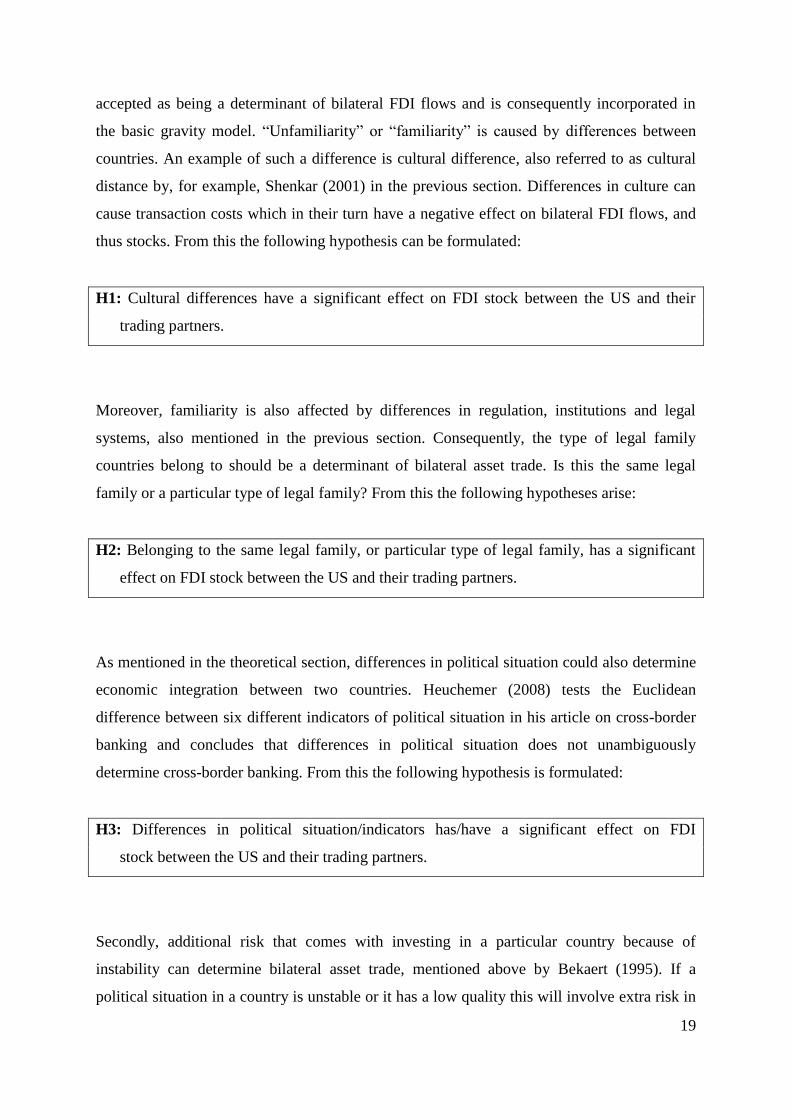
thus stocks. From this the following hypothesis can be formulated:

H1: Cultural differences have a significant effect on FDI stock between the US and their

trading partners.

Moreover, familiarity is also affected by differences in regulation, institutions and legal

systems, also mentioned in the previous section. Consequently, the type of legal family

countries belong to should be a determinant of bilateral asset trade. Is this the same legal

family or a particular type of legal family? From this the following hypotheses arise:

H2: Belonging to the same legal family, or particular type of legal family, has a significant

effect on FDI stock between the US and their trading partners.

As mentioned in the theoretical section, differences in political situation could also determine

economic integration between two countries. Heuchemer (2008) tests the Euclidean

difference between six different indicators of political situation in his article on cross-border

banking and concludes that differences in political situation does not unambiguously

determine cross-border banking. From this the following hypothesis is formulated:

H3: Differences in political situation/indicators has/have a significant effect on FDI

stock between the US and their trading partners.

Secondly, additional risk that comes with investing in a particular country because of

instability can determine bilateral asset trade, mentioned above by Bekaert (1995). If a

political situation in a country is unstable or it has a low quality this will involve extra risk in

20

investing in that country. I think that risk that is caused by instability is of more value in

explaining FDI stock, than risk that is caused by “unfamiliarity” with a different particular

political situation. So, I will test the six different political indicators which are also used by

Heuchemer, but instead of measuring the difference between two countries, I will measure

the rank or quality of that political indicator and see if it is significant in determining bilateral

FDI stock between the US and its partner countries. From this the following hypothesis can

be formulated:

H4: The quality of the political situation/indicators in a country does not has/have a

significant effect on FDI stock between the US and their trading partners.

21

3. METHODOLOGY

This chapter will discuss the empirical approach to test the hypotheses. Accordingly,

the data and variables used are discussed and incorporated in the model.

3.1 Variables explained

For this research a new dataset is constructed by gathering and combining data from different

sources.

FDI

As dependent variable we use in our model foreign direct investment data from OECD‟s

international direct investment database. The OECD‟s database provides nominal bilateral

FDI inward and outward stock of the US to and from its partner countries (country i). In this

research annual data of 37 partner countries over the period 1985-2006 were used. So we

have a total of 814 observations (37x21). To obtain the total FDI position between the US

and a partner country inward and outward stock has been added up. Because e few data

points were missing we extrapolated some years for some countries. So, three different

variables will be explained: total FDI, inward FDI and outward FDI. Total FDI is the sum of

inward and outward FDI.

GDP per capita

As mentioned in the theoretical part, the gravity equation is the most frequently used

workhorse for resolving bilateral investment flows and positions, and possibly the best way to

study the effect of third factors, such as cultural an political differences. In the gravity

equation model economic masses of both trading countries are used to explain investment

flows. So in our research we also use GDP of both US and its partner country. We expect the

sign of both US and partner country GDP to be positive.

GDP per capita acts as a proxy for relative factor endowments. Thus a positive coefficient for

β2 indicates that bilateral trade is inter-industry and driven by comparative advantage as

suggested by the “old” trade theory of the Ricardo-Heckscher-Ohlin-Samuelson type. In

contrast, a negative value for β2 would indicate support for the Linder hypothesis which

22

suggests that trade volumes are larger the more similar the trading partners are in terms of

factor proportions and thus development. (Heuchemer, 2008)

Population

Population is also used in a gravity equation. Population acts as a proxy for size of a country

and in combination with GDP per capita economic mass is represented in the model. We

expect the sign of both US and partner country population to be positive.

Distance

Geographical distance is considered to be a proxy of bilateral transaction costs. Firstly,

because geographical distance increases transportation costs for people traveling to a distant

country to monitor their investment, especially in the case of FDI, which is highly

information sensitive. Secondly, because geographical distance increases unfamiliarity and

information asymmetries. Distance is measured between the US capital and its partner

country‟s capital. We expect the sign of distance to be negative.

Border

Border is a dummy variable which captures shows the existence of a common border between

the US and the partner country. We expect the sign of a common border to be negative.

Language

In a gravity model it is also a common strategy to use a dummy variable for the existence of a

common language. Because a common language induces familiarity and facilitates

monitoring, we expect the sign to be positive.

Trade

Trade is the sum of import and export between the US and partner countries. Trade can

induce familiarity, which decreases information asymmetries and increases FDI investments

between countries. On the other hand trade and FDI flows can also act as substitutes. Because

of this ambiguity it will be difficult to predict whether the sign of trade will be positive or

negative. However, literature has shown that trade is likely to be positive.

23

Market Capitalization

Market capitalization is an important factor in FDI research, because when using a gravity

approach it is not only important to know the market size but also to which extent this market

is capitalized. A country with a high market capitalization will be able to generate more

capital to invest in FDI abroad. Hence, market capitalization in each country is an

endogenous variable in the model. higher asset price is implied by higher aggregate demand

from foreign countries, which in turn increases the incentives of agents to start new risky

projects and list more financial assets. Furthermore, it also offers more investment

opportunities to foreign countries, in which to invest FDI in. So market capitalization is

expected to have a positive sign.

Tax Rate

Corporate tax rates decrease returns in FDI, which takes away incentives to invest in a

foreign country with high corporate tax rates. So tax rate is expected to have a negative sign.

Tax Treaty

Tax treaty is a mutual agreement or bilateral contract of countries to lower tax for each other.

Tax treaty is a dummy variable which is expected to have a positive sign.

Legal Family

In our regression model we estimate two different legal family variables. The first one

Legalfam01 is a dummy variable which indicates if a partner country belongs to the same

legal family as the US. We expect the sign of this parameter to be positive due to a familiarity

effect. The second variable is Legalfam and indicates to which legal family a partner country

belongs. The options are Scandinavian, French, German and English (same as US). This

dummy is successfully applied in La Porta et al. (1998).

Cultural Differences

Cultural differences are measured as Euclidean distance and are derived from Hofstede‟s four

cultural dimensions and have also been used to examine in Heuchemer et al. (2008).

Hofstede‟s four cultural dimensions are based on the result of a broad questioning in more

than 50 countries. Hofstede (1980) conducted a factor analysis to identify four different

dimensions that can be used to describe national cultures. It is a measure that figures

prominently in the management literature. These four dimensions are:

24

“Power Distance Index (PDI) that is the extent to which the less powerful members of

organizations and institutions (like the family) accept and expect that power is distributed

unequally. This represents inequality (more versus less), but defined from below, not from

above. It suggests that a society's level of inequality is endorsed by the followers as much as

by the leaders.” (Hofstede, 1980)

“Individualism (IDV) on the one side versus its opposite, collectivism, that is the degree to

which individuals are integrated into groups. On the individualist side we find societies in

which the ties between individuals are loose: everyone is expected to look after him/herself

and his/her immediate family. On the collectivist side, we find societies in which people from

birth onwards are integrated into strong, cohesive in-groups, often extended families (with

uncles, aunts and grandparents) which continue protecting them in exchange for

unquestioning loyalty.” (Hofstede, 1980)

“Masculinity (MAS) versus its opposite, femininity, refers to the distribution of roles between

the genders which is another fundamental issue for any society to which a range of solutions

are found. The IBM studies revealed that (a) women's values differ less among societies than

men's values; (b) men's values from one country to another contain a dimension from very

assertive and competitive and maximally different from women's values on the one side, to

modest and caring and similar to women's values on the other.” (Hofstede, 1980)

“Uncertainty Avoidance Index (UAI) deals with a society's tolerance for uncertainty and

ambiguity; it ultimately refers to man's search for Truth. It indicates to what extent a culture

programs its members to feel either uncomfortable or comfortable in unstructured situations.

Unstructured situations are novel, unknown, surprising, different from usual. Uncertainty

avoiding cultures try to minimize the possibility of such situations by strict laws and rules,

safety and security measures, and on the philosophical and religious level by a belief in

absolute Truth; 'there can only be one Truth and we have it'. People in uncertainty avoiding

countries are also more emotional, and motivated by inner nervous energy. The opposite type,

uncertainty accepting cultures, are more tolerant of opinions different from what they are

used to; they try to have as few rules as possible, and on the philosophical and religious level

they are relativist and allow many currents to flow side by side. People within these cultures

25

are more phlegmatic and contemplative, and not expected by their environment to express

emotions.” (Hofstede, 1980)

According to the scores of Hofstede‟s factor analysis, each country can be characterized by a

score on each of the four dimensions and these scores are the basis for the cultural proxy in

our analysis. As mentioned above cultural differences are measured as Euclidean distance.

We expect the parameter sign to be negative as a consequence of a high cultural distance

increasing information asymmetry.

Political Indicators

Political differences are expressed in six different political or governance factors.

The World bank defines these six different dimensions of governance and constructs these in

units ranging from about -2.5 to 2.5, with higher values corresponding to better governance

outcomes. The governance dimensions are also ranked on a scale from 0 to 100. Six political

dimensions are defined: voice and accountability (VA), political stability and absence of

violence (PSNV), government effectiveness (GE), regulatory quality (RQ), rule of law (RL),

and control of corruption (CC). We calculate these dimensions in Euclidean distances

Furthermore, we also aggregate all these dimensions into an overall political risk proxy

(POLITICAL) that measures the general political dissimilarity between countries in one

Euclidean distance. Besides the calculation in Euclidean distances we also use political

variables in our regression model based on a partner country‟s rank on a political dimension

measurement list scaling from 0 to 100. So the partner country‟s performance is measured in

a specific governance dimension instead of its Euclidean difference with the US. Six political

dimensions are defined: voice and accountability rank (VAR), political stability and absence

of violence rank (PSNVR), government effectiveness rank (GER), regulatory quality rank

(RQR), rule of law rank (RLR), and control of corruption rank(CCR). Again we also

aggregate all these dimensions into an overall political risk proxy (POLITICALR) that

measures the general political performance of a country. The political variables measured in

Euclidean distance are expected to have a negative sign because with Euclidean distance

unfamiliarity increases and information asymmetry rises. The political variables measured in

ranks are expected to have a positive sign because a high value indicates a good performance

of a partner country on that particular dimension. A good performance in political indicators

implicates lower risk of an possible investment and could increase FDI.

26

3.2 Model

In this section we try to outline the functional forms of the models to be estimated and

furthermore we try to define the variables which best fit the models. The model will be

analyzed as panel data, sometimes called longitudinal data, which is analyzed differently as

pure cross sectional data or pooled cross sectional data, because country specific factors can

influence the dependent variable and the sample that is analyzed concern data for the same

country over time.

Moreover, an equation has to be defined to analyze the FDI flows over time. As mentioned in

the theoretical paragraph empirical literature shows that gravity equations are used to model

trade flows. The gravity equation is the most frequently used workhorse for resolving

bilateral investment flows and positions and possibly the best way to study the effect of third

factors, like cultural an political differences. In the gravity equation model economic masses

of both trading countries are used to explain investment flows.

In addition to the economic masses, geographical distance (DISTANCE) is also incorporated

in the regression equation. The model is completed by the gravitational constant (G):

Xijt = G ²DISTANCE

GDPGDP

ij

jtit (1)

where Xijt is defined as bilateral asset trade of country i to country j in year t. To arrive at the

regression model the gravity equation is converted into a linear relationship between the

explanatory variables and the trade flows, in this case, FDI flows. A logarithmic version of

the regression model is shown:

ln(Xijt) = x0 + β1 lnGDPit + β2 lnGDPjt + β3 lnDISTANCEij (2)

This is the essence of the gravity model but in the empirical literature more variations and

extensions of the basic gravity model are presented. We will show and test these variations

and extensions after which we will use the model that will best fit our data.

27

A popular version of the gravity equation used in the empirical trade literature, we find in

Baltagi (2003):

lnXijt = x0 + β1lnSIZEijt + β2lnRELijt + β3lnSIMILARijt + β4lnDISTANCEij + β5BORDERij

+

K

6k

βklnYijt + uijt (3)

Baltagi derives the variables SIZE, REL and SIMILAR from the advances of trade theory

presented by Krugman (1980) and Helpman & Krugman (1985). Size represents the

economic masses of both trading partners and is defined as the product or the sum of the

GDPs of the trading partners. REL represents the difference in economic welfare of the

trading partners measured in GDP per capita (GDPpc) and serves as a proxy for relative

factor endowments and possibly a level of familiarity.

SIMILAR is defined as a similarity index of both trading countries‟ GDP and serves as a

proxy for relative country size. Baltagi expands the gravity model with the dummy variable

BORDER, which represent an adjacent country. The remainder stochastic disturbance is

represented by uijt

Guerin (2006) also presents a gravity equation in has article in which he tries to explains FDI

flows. He specifies the following model:

Inflwijt = a + β1 lnPOPit + β2 lnGDPpcit + β3 lnDISTij + β4Zij + tt + dj + eij,t (4)

In this gravity equation country size is measured as POP which represents the population in a

partner country. Economic prosperity is again measured in GDPpc and also distance is

incorporated in the model by Guerin. These variables are in logs, therefore the coefficients

can be interpreted as semi-elasticities. A set of control variables are added to the model, Zij,

time dummies, tt, source country dummies, dj, and the remainder stochastic disturbance i.e.

the error term, eij,t.

Portes and Rey (2005) use a gravity model in his article on asset trade and arrives at the next

model:

28

logTij = k1log(MiMj) + k2log(τij) + k3 (5)

Mi and Mj represent the economic masses of country i and country j. In this equation

economic masses are measured as equity market capitalizations. τij represents the transaction

cost between the trading partners. k1<0, k2<0 and k3 are constants to be estimated.

These models will be tested combined and separately, to arrive at the best-fit model for our

data, which will be used to estimate the parameters of the variables.

In principle this baseline model that we will be using could be estimated by OLS. However,

the estimation results could possibly be biased due to omitted variable effects (Heuchemer,

2008). These omitted variable effects could represent effects that are similar to all country

pairs (i) but specific to any year (t) and effects (ii) that are country pair specific but similar

for all years respectively. Therefore, panel data techniques should be applied and the error

term will be defined as follows:

uijt = λij + τt + εijt (6)

In this equation the error term is explained by λij, which reflects any time invariant bilateral

idiosyncratic effect, and τt, which captures the time effect. The equation is completed with an

error term.

These unobserved effects can be considered as fixed or random. Therefore, the unobserved

time effect can be considered as fixed. To control for events, possible trends or aggregate

shocks, such as world business cycles movements, global capital market shocks or

movements in the world rate of interest year dummies are included in the model.

Incorporating year dummies in the model allows the intercept of the equation to change over

time and is able to correct for trends over time. The equation above contains the unobservable

time effect or fixed effect, τt, where the subscript t stands for year t. λij can de considered as a

separate intercept to be estimated for each country; it is the country fixed effect. There could

be time specific factors which are constant over different countries, which influence the

dependent variable. These factors are obtained in λij.

29

To analyze panel data with unobserved effects a Least Squared Dummy Variable Model

(LSDV) is used. This method generates results that are corrected for country and time

specific effects and errors.

This fixed effects model allows us to analyze panel data using OLS and meanwhile obtaining

comparable results which would be obtained using pure cross sectional data (Wooldridge,

2002).

We expect that the specifications above will capture a substantial amount of variance in the

data. However, the fixed effects approaches are not able to estimate models which contain

time invariant variables, such as border, distance, language or the political and cultural

factors, in which we are interested. They are also unable to estimate models which contain

country invariant variables, such as population of the US and GDP per capita of the US. So

these fixed effects approaches will be used estimating country and time variant variables for

their robustness. We will check for robustness by experimenting with various control

variables, normalizations and dummies, which are common in asset trade to arrive at the best

conclusion

Furthermore, in our model a substantial amount of country specific differences are measured,

most of those variables act as a proxy for political and cultural differences, which are non-

time varying. These political and cultural variables are measured as Euclidean distances

between two countries:

ED =

K

1k

jtkitk VV ² (7)

ED defines Euclidean distance and V are the different variable that are taken into account of

country i and of country j.

The modelling strategy is thus as follows: First we develop a baseline gravity equation

employing the pure trade-theoretic explanatory variables and estimate these different

variables, after which we will define a basic gravity model that best fits our data. Secondly,

this model is extended with two more variables that are also often used in empirical asset

30

trade models and we check the robustness of the variables incorporated in the first model.

Thirdly, the augmented model is extended with cultural and political variables separately and

run Wald-tests to test the significance of each of these variables. Time and country non-

varying variables will be left out of the model and fixed and random panel effects will be

tested. Fourthly, all the variables are incorporated to be tested into the gravity model and

again these variables will be tested, running Wald-tests. Fifthly, we leave time and country

non-varying variables out of the model and test fixed and random panel effects.

Because of the absence of a clear theoretical foundation the model is empirically tested and

the variables which best fit our data are selected and placed into the model.

3.3 Gravity equations

Different gravity equations are defined to test the effect and robustness of the models and

explaining variables.

3.3.1 Basic gravity equation

Different models and variables were tested such as GDP, population and GDP per capita for

both the US and trading partners. The most appropriate model incorporates population and

GDP per capita as shown below. Implicitly this means that GDP is also represented in the

model, however population and GDP per capita better fit our data. All variables were also

tested with and without log and the most significant was selected. After adding Distance,

Border and Language to the gravity model this resulted in the following basic benchmark

gravity equation:

lnFDIit = β0 + β1lnPopust + β2lnPopit + β3lnGDPpcust + β4lnGDPpcit + β5Distancei +

β6Borderi + β7Languagei + εit (8)

i = 1,…, N ; t = 1,…, T,

Whereby N is the number of countries and T the number of years, εit is the remainder

stochastic disturbance, εit ~ IID (0, )

31

3.3.2 Augmented gravity equation

By adding log Trade and log Market cap to the basic gravity equation we developed the

augmented gravity equation. Trade and Market cap are frequently used explaining variables

in the empirical asset trade literature and also add significance to our model.

This leads to the following augmented gravity equation:


β6Borderi + β7Languagei + β8lnTradeit + β9lnMarketcapit + εit (9)

i = 1,…, N ; t = 1,…, T,

Using this model we also test the robustness of the basic gravity model.

3.3.3 Augmented gravity equation including explaining variables

separately

Explaining variables are added to the augmented gravity equation separately to test if they are

significant and add value to the model running Wald-tests. Y represents the following

variables: TaxRate, TaxTreaty, LegalFam, LegalFam01, Culture, Political, VA, PSNV, GE,

RQ, RL, CC, VAR, PSNVR, GER, RQR, RLR and CCR


β6Borderi + β7Languagei + β8lnTradeit + β9lnMarketcapit + β10Y + εit (10)

i = 1,…, N ; t = 1,…, T,

3.3.4 Total gravity equation including all explaining variables

I will conclude specifying the total model including all explaining variables that were tested

above. Again we will run Wald-tests to test if the different variables are significant in the

extended model.

32


β6Borderi + β7Languagei + β8lnTradeit + β9lnMarketcapit + β10TaxRatei + β11TaxTreatyi +

β12LegalFam01i + β13Culturei + β14VAi + β15PSNVi + β16GEi + β17RQi + β18RLi + β19CCi + εit

i = 1,…, N ; t = 1,…, T, (11)

3.3.5 Time and country fixed effects model

In this model all time and country non-varying variables are left out of the model to test time

and country-fixed effects. The following model is specified to test time-fixed effects:

lnFDIit = β0 + β1lnPopit + β2lnGDPpcit + β3Distancei + β4Borderi + β5Languagei + β6lnTradeit +

β7lnMarketcapit + β8TaxRatei + β9TaxTreatyi + β10LegalFam01i + β11Culturei + β12VAi +

β13PSNVi + β14GEi + β15RQi + β16RLi + β17CCi + τt + εit

i = 1,…, N ; t = 1,…, T, (12)

The following model is specified to test country-fixed effects:

lnFDIit = β0 + β1lnPopust + β2lnPopit + β3lnGDPpcust + β4lnGDPpcit + β5lnTradeit +

β6lnMarketcapit + λi + εit

i = 1,…, N ; t = 1,…, T, (13)

33

4. RESULTS

In this chapter the results of the regression models will be explained, according to the

equations discussed in the methodology. After which, the estimated parameters of the

political and cultural factors are explained. On from this, a Wald test and robustness check

will be carried out to test the significance and the robustness of the political and cultural

parameters. The chapter is concluded with a discussion of the results.

4.1 Results

The models are discussed in the same sequence as in the methodology. First the basic gravity

model is explained

4.1.1 Basic gravity model

Table 4.1: Basic Gravity ModelMethod: Panel Least Squares Panel Least Squares Panel Least Squares

Sample: 1985-2006 1985-2006 1985-2006

Periods included: 22 22 22

Cross-sections included: 37 37 37

Total panel observations:814 814 814

Dependent variable: ln(Total FDI Stock) ln(Inward FDI Stock) ln(Outward FDI Stock)

Coefficiënt Probability Coefficiënt Probability Coefficiënt Probability

C -320,2688 0,000 -364,4429 0,000 -305,7848 0,000

lnGDPPC 1,3719 0,000 2,3303 0,000 1,0666 0,000

lnPOP 0,8305 0,000 1,1079 0,000 0,7154 0,000

lnGDPPCUS -7,5772 0,000 -10,2759 0,000 -6,8859 0,001

lnPOPUS 30,8127 0,000 35,5072 0,000 29,3685 0,000

BORDER 1,0036 0,000 0,6882 0,001 1,1940 0,000

DISTANCE 0,0003 0,019 -0,0002 0,180 0,0003 0,002

LANGUAGE 0,8853 0,000 0,9605 0,000 1,0016 0,000

R-squared 0,7135 0,792 0,661

Adjusted R-squared 0,7110 0,790 0,658

S.E. of regression 0,9820 1,222 0,961

Sum squared resid 777,2803 1117,754 740,224

Log likelihood -1136,2290 -1220,529 -1111,983

F-statistic 286,7927 405,987 223,245

Prob(F-statistic) 0,0000 0,000 0,000

The results of the basic regression model are shown in table 1. With the exception of the

Constant (C) and GDPpc US all parameter signs are positive. This implies that those

variables have a positive effect on asset trade between the US and its partner countries, both

on inward and outward side. As mentioned above GDPpc US has a negative effect on both

inward and outward stock of FDI. Thus, an increase of economic growth in the US causes a

34

decrease of FDI stock between the US and their partner countries. While economic growth in

the partner country has a positive effect on bilateral FDI stocks.

Another remarkable observation is the positive parameter of distance, implying that

investments between countries increase if countries are more distant. This could be a

consequence of FDI being a substitute for trade. With distance transportation costs rise and it

becomes cheaper for a MNE to produce abroad and for example invest in a subsidiary

company, which increases FDI. The fact that especially outward FDI stock is significantly

influenced by distance emphasizes this argument, because profitability of producing abroad

depends on costs and especially labour costs. In contrary to the US, where labour costs are

relatively high and so partner countries are less likely to decide to produce in the US and

consequently inward FDI stock is insignificant.

With exception of distance for total FDI stock and inward FDI stock, all signs are significant

at a 1% level of significance. 71% of total FDI stock, 79% of inward FDI stock and 66% of

outward FDI stock is explained by the gravity equation. So, the basic gravity has more value

explaining inward FDI stock than outward FDI stock.

4.1.2 Augmented gravity model

Table 4.2: Augmented Gravity ModelMethod: Panel Least Squares Panel Least Squares Panel Least Squares

Sample: 1985-2006 1985-2006 1985-2006






C -270,3553 0,000 -324,1920 0,000 -259,5891 0,000

lnGDPPC 0,7929 0,000 1,7451 0,000 0,5611 0,000

lnPOP 0,3419 0,000 0,5421 0,000 0,2723 0,000

lnGDPPCUS -7,1587 0,000 -10,0437 0,000 -6,3707 0,000

lnPOPUS 26,7540 0,000 32,4387 0,000 25,5000 0,000

BORDER -0,4379 0,004 -0,9547 0,000 -0,1218 0,443

DISTANCE -0,0003 0,002 -0,0007 0,000 -0,0001 0,174

LANGUAGE 0,5517 0,000 0,5866 0,000 0,7201 0,000

lnTRADE 0,6494 0,000 0,7695 0,000 0,5968 0,000

lnMARKETCAP 0,1625 0,000 0,0194 0,625 0,1158 0,000

R-squared 0,8164 0,841 0,756


S.E. of regression 0,7871 1,069 0,817


Log likelihood -955,1598 -1117,865 -979,312

F-statistic 397,2367 439,065 274,895

Prob(F-statistic) 0,0000 0,000 0,000

35

In the augmented gravity model lnTrade and lnMarketcap variables have been added to the

model to increase the model‟s fit. R-squared increases after adding both variables to 82%,

84% and 76% for total FDI stock, inward FDI stock and outward FDI stock respectively, an

overall increase of approximately 10%. Trade and Market Capitalization have obviously a

great explaining value. Both variables are significant at a 1% significance level. Except for

inward stock, the market capitalization of the partner country is not significant. This suggests

that market capitalization of a receiving country is an important explaining factor for FDI and

not the market capitalization of the investing country. Also, the sign of Trade is positive

possibly because of the theory, as explained before, that trade increases familiarity and

consequently familiarity induces investments. When adding Trade and Market capitalization

to the model all signs of the remaining variables stay the same except for border and distance

which change from positive to negative. This is probably caused by the correlation between

trade and both border and distance. When border and distance are corrected for trade only a

negative effect remains, meaning that sharing a border and being distant to a partner

decreases FDI. This is probably due to the possibility of FDI being a substitute for trade. This

effect is only observed for inward FDI stock and total FDI stock. In the augmented gravity

equation border and distance are insignificant for outward FDI stock at a 10% significance

level.

4.1.3 Augmented gravity model including explaining variables

separately

The explaining variables will be implemented into the augmented gravity model separately

and the results will also be discussed separately per variable. With exception of legal family,

culture and the separate political indicators: VA, PSNV, GE, RQ, RL and CC. These are

discussed at the end of this chapter when they are analyzed for all models together.

Tax rate

Tax rate is not significant in explaining total FDI stock at a 10% significance level. Tax rate

is significant in explaining inward FDI stock at a 1% significance level and outward FDI

stock at a 5% significance level. The sign of the tax rate for inward FDI is positive. Hence,

the higher a corporate tax level in a partner country, the higher the FDI stock to the US from

that country. As a consequence of a high corporate tax level at home, countries invest more

36

abroad. The sign of the tax rate parameter for outward FDI stock is negative as investing in a

partner country becomes more expensive with higher corporate tax levels and consequently

FDI decreases.

Tax Treaty

Tax treaty is significant in explaining total FDI stock and inward FDI stock at a 5%

significance level and it is significant in explaining outward FDI stock at a 1% significance

level. Looking at total and outward FDI stock a tax treaty has a positive effect on FDI which

is in line with the theory that tax breaks have positive effect on investments. The augmented

gravity model, however, shows that a tax treaty has a negative effect on inward FDI stock,

which suggests that partner countries invest less in the US if there exists a tax treaty between

these countries.

Political Difference

The political variable representing the difference between the US and a partner country on all

six aspects of political situation in a country is significant for total and outward FDI stock at a

5% significance level. In explaining inward FDI stock political variable is insignificant. The

sign shown by the augmented gravity model for the parameter is positive. This is remarkable

because it suggests that the more different political situations in a country are the investments

it breeds, whereas we would expect that similar situations increase familiarity and as a

consequence increases investments. The US invests in countries which have a substantial

different political situation. An explanation could be that political difference is of less

importance than political quality or rank. Higher quality or a higher rank means more

stability and less risk. Investment risk increases costs and decreases investment. In three of

the six political indicators the US takes a relatively low rank which means more or less

political instability. Countries that represent a high rank have a different political situation as

the US but are an attractive country, in which to inves, so in this case more political

difference could mean more FDI outward stock. This is emphasized by the fact that outward

stock is significant and inward stock is not. We will have a closer look at this below where

we will explain the different political indicators separately.

Political Rank

The variable indicating the quality of the political situation in a partner country of the US

measured by six different indicators is significant in the inward FDI stock model at a 5%

37

significance rate and in the outward at a 1% significance rate. The political rank variable is

insignificant in the total FDI stock model. First, in the inward FDI stock model the sign of the

political rank parameter is positive indicating that countries with a high rank or quality of

total political situation will invest more FDI in the US than countries that have a low rank or

quality of total political situation. In general, countries with better developed governments

and institutions are better facilitated in investing abroad. Secondly, in the outward FDI stock

model the sign of the political rank parameter is negative indicating that the US invests more

FDI in countries with a low quality or rank of total political situation. This suggests a strong

weight of vertical FDI flows from the US to abroad relative to the total amount from the US

to abroad. Vertical FDI flows take place especially from developed to developing country.

4.1.4 Total model including all explaining variables

In this paragraph four different models are shown. An important advantage of showing four

models is that we can test robustness of the parameters. In all four models all variables are

included. They only differ in the following aspects:

Model 3 (Table 4.3): Political indicators measured in differences and Legalfam are included.


Model 5 (Table 4.5): Political indicators measured in ranks and Legalfam are included.

Model 6 (Table 4.6): Political indicators measured in ranks and Legalfam01 are included.

38

Table 4.3: Total Gravity Model; including Legal Family and Political Difference indicatorsMethod: Panel Least Squares Panel Least Squares Panel Least Squares

Sample: 1985-2006 1985-2006 1985-2006






C -277,3015 0,000 -295,2990 0,000 -283,5315 0,000

lnGDPPC 0,8055 0,000 1,4855 0,000 0,6597 0,000

lnPOP 0,2283 0,000 0,4054 0,000 0,1363 0,027

lnGDPPCUS -7,5764 0,000 -8,7367 0,000 -7,4135 0,000

lnPOPUS 27,7465 0,000 29,3791 0,000 28,3386 0,000

BORDER -0,3660 0,059 -0,2846 0,250 -0,0510 0,794

DISTANCE 0,0001 0,343 -0,0005 0,001 0,0004 0,000

LANGUAGE -0,1229 0,338 -0,0805 0,637 -0,0329 0,799

lnTRADE 0,7554 0,000 0,7936 0,000 0,7208 0,000

lnMARKETCAP 0,1337 0,000 -0,0394 0,344 0,0850 0,008

TAXRATE -0,0002 0,033 0,0002 0,068 -0,0003 0,000

TAXTREATY 0,0506 0,713 -0,6511 0,000 -0,0293 0,833

LEGALFAM -0,1189 0,024 0,0151 0,830 -0,1904 0,000

CULTURE -0,0151 0,000 -0,0130 0,000 -0,0167 0,000

VA -0,00001 0,086 -0,00003 0,002 -0,00001 0,073

PSNV -0,000001 0,855 0,00003 0,005 -0,00003 0,000

GE 0,0001 0,000 -0,0001 0,000 0,0001 0,000

RQ 0,00003 0,085 0,0001 0,000 0,00003 0,094

RL -0,00005 0,002 -0,0001 0,000 -0,00003 0,031

CC 0,000003 0,842 0,0001 0,000 -0,00003 0,030

R-squared 0,842 0,884 0,805


S.E. of regression 0,730 0,910 0,733


Log likelihood -864,578 -9623,344 -862,161

F-statistic 216,093 286,952 166,182

Prob(F-statistic) 0,000 0,000 0,000

Table 4.4: Total Gravity Model; including Legal Family 01 and Political Difference indicatorsMethod: Panel Least Squares Panel Least Squares Panel Least Squares

Sample: 1985-2006 1985-2006 1985-2006






C -239,3739 0,000 -273,4102 0,000 -251,6227 0,000

lnGDPPC 0,4809 0,000 1,3217 0,000 0,3840 0,000

lnPOP 0,1146 0,047 0,3370 0,000 0,0448 0,459

lnGDPPCUS -6,2155 0,000 -7,9900 0,000 -6,2689 0,000

lnPOPUS 23,9064 0,000 27,1894 0,000 25,0968 0,000

BORDER -0,0245 0,890 -0,1348 0,575 0,2823 0,130

DISTANCE 0,0004 0,000 -0,0004 0,006 0,0008 0,000

LANGUAGE 0,5075 0,000 0,1917 0,244 0,5345 0,000

lnTRADE 0,7994 0,000 0,8113 0,000 0,7636 0,000

lnMARKETCAP 0,2070 0,000 0,0050 0,903 0,1462 0,000

TAXRATE -0,0002 0,001 0,0002 0,060 -0,0003 0,000

TAXTREATY -0,4702 0,000 -0,8995 0,000 -0,5010 0,000

LEGALFAM -1,2132 0,000 -0,7215 0,000 -0,9079 0,000

CULTURE -0,0242 0,000 -0,0181 0,000 -0,0248 0,000

VA 0,00001 0,112 -0,00002 0,160 0,00001 0,475

PSNV 0,00002 0,008 0,00004 0,000 -0,00001 0,092

GE 0,00002 0,317 -0,0001 0,000 0,0001 0,000

RQ 0,0001 0,000 0,0002 0,000 0,0001 0,000

RL -0,0001 0,000 -0,0001 0,000 -0,00005 0,001

CC -0,00004 0,000 0,0001 0,000 -0,0001 0,000

R-squared 0,863 0,888 0,817


S.E. of regression 0,679 0,896 0,710


Log likelihood -806,759 -9505,302 -836,647

F-statistic 256,451 297,559 180,018


39

Table 4.5: Total Gravity Model; including Legal Family and Political Rank indicatorsMethod: Panel Least Squares Panel Least Squares Panel Least Squares

Sample: 1985-2006 1985-2006 1985-2006






C -285,3985 0,000 -287,3239 0,000 -296,8237 0,000

lnGDPPC 0,8229 0,000 1,4107 0,000 0,7966 0,000

lnPOP 0,3402 0,000 0,3390 0,000 0,4068 0,000

lnGDPPCUS -8,1606 0,000 -8,9919 0,000 -8,1486 0,000

lnPOPUS 28,7541 0,000 28,8700 0,000 29,7567 0,000

BORDER -0,0668 0,680 -0,9346 0,000 0,4348 0,009

DISTANCE 0,0010 0,000 0,0002 0,348 0,0012 0,000

LANGUAGE 0,1995 0,117 0,4852 0,010 0,3035 0,020

lnTRADE 0,8729 0,000 1,0207 0,000 0,7226 0,000

lnMARKETCAP 0,1468 0,000 -0,0060 0,883 0,1262 0,000

TAXRATE -0,0005 0,000 -0,0002 0,065 -0,0007 0,000

TAXTREATY 0,0597 0,650 -0,7217 0,000 0,0289 0,831

LEGALFAM -0,1219 0,004 0,0588 0,359 -0,2542 0,000

CULTURE -0,0060 0,004 -0,0089 0,005 -0,0041 0,050

VA 0,0255 0,000 0,0307 0,000 0,0248 0,000

PSNV 0,0001 0,970 -0,0132 0,000 0,0029 0,169

GE -0,0648 0,000 0,0127 0,138 -0,0683 0,000

RQ -0,0272 0,000 -0,0510 0,000 -0,0284 0,000

RL 0,0180 0,002 0,0262 0,005 0,0089 0,142

CC 0,0365 0,000 -0,0019 0,887 0,0450 0,000

R-squared 0,870 0,880 0,833


S.E. of regression 0,663 0,927 0,677


Log likelihood -788,108 -9756,409 -799,376

F-statistic 270,778 275,396 201,913


Table 4.6: Total Gravity Model; including Legal Family 01 and Political Rank indicatorsMethod: Panel Least Squares Panel Least Squares Panel Least Squares

Sample: 1985-2006 1985-2006 1985-2006






C -266,8515 0,000 -286,5920 0,000 -284,6221 0,000

lnGDPPC 0,6484 0,000 1,4034 0,000 0,6711 0,000

lnPOP 0,2365 0,000 0,3289 0,000 0,3486 0,000

lnGDPPCUS -7,5245 0,000 -8,9376 0,000 -7,7686 0,000

lnPOPUS 26,9029 0,000 28,7858 0,000 28,5450 0,000

BORDER -0,2919 0,082 -0,9422 0,000 0,2747 0,120

DISTANCE 0,0009 0,000 0,0001 0,460 0,0012 0,000

LANGUAGE 0,5303 0,000 0,4318 0,014 0,7122 0,000

lnTRADE 0,9317 0,000 1,0164 0,000 0,7812 0,000

lnMARKETCAP 0,1641 0,000 -0,0098 0,810 0,1420 0,000

TAXRATE -0,0004 0,000 -0,0002 0,096 -0,0006 0,000

TAXTREATY -0,0555 0,677 -0,7203 0,000 -0,0659 0,637

LEGALFAM -0,3900 0,001 -0,0778 0,642 -0,1108 0,343

CULTURE -0,0093 0,000 -0,0094 0,009 -0,0051 0,029

VA 0,0197 0,000 0,0300 0,000 0,0219 0,000

PSNV -0,0036 0,075 -0,0125 0,000 -0,0017 0,426

GE -0,0567 0,000 0,0153 0,108 -0,0689 0,000

RQ -0,0201 0,002 -0,0510 0,000 -0,0217 0,002

RL 0,0170 0,004 0,0268 0,004 0,0067 0,281

CC 0,0313 0,001 -0,0036 0,792 0,0451 0,000

R-squared 0,870 0,880 0,826


S.E. of regression 0,661 0,927 0,691


Log likelihood -786,150 -9759,628 -816,243

F-statistic 272,322 275,121 191,747


40

If we compare those four models we see that the best fit or the highest R-squared (adjusted) is

produced in model 6, namely 0.867%, followed by model 5, model 4 and model 3, with

0.866%, 0.860% and 0.838% respectively. This proves that political ranks over political

differences explain the data more precisely. In addition, Legalfam01 fits the data more

precise than Legalfam shown by the adjusted R-squared.

If we have a closer look at the different explaining variables and compare the four different

extended models we see that the first five explaining variables in the model: C, lnGDPpc,

lnPop, lnGDPpcUS and PopUS have approximately the same parameter and are all

significant, with the exception of lnPop in model 3 and 4. This shows that the first five

parameters in the model are rather robust.

If we do the same for the variable border we see that border is not significant in every model,

but has the same signs in all models, with the exception of the outward FDI stock model 3.

Sharing a border has a positive effect on outward FDI stock and a negative effect on total and

inward FDI stock.

Distance has in all four models a positive effect on total and outward FDI stock. In models

(5&6) including the political rank variables distance also has a positive effect on inward FDI

stock but in models (3&4) including the political difference variables it has a negative effect

on inward FDI. So distance has a positive effect on total and outward FDI stock but the effect

on inward FDI stock is ambiguous. In addition, distance is in almost every model significant.

Language is in all models significant, except for model 3. In the remaining models language

has an unambiguous positive effect on FDI stock.

lnTrade is in all models significant and has a positive effect on FDI stock between the US and

partner countries.

LnMarketCap of a partner country is in all models significant in explaining total and outward

FDI stock on which it has a positive effect. So market capitalization of a particular country

41

explains, according our model, FDI to that particular country and not from that particular

country.

The corporate tax rate of a partner country has a negative effect on total and outward FDI

stock and the effect on inward FDI stock is ambiguous and insignificant and depending on

the model.

The existence of a tax treaty between the US and its partner country is only significant in all

models explaining inward FDI stock, in which it has a negative effect. Only in model 4 does

it have a significant effect on total and outward stock and also for these explained variables

the effect is negative.

4.1.5 Time and country fixed effects models

In this paragraph five different fixed effects models are shown. An important advantage of

showing these five models is that we can test robustness of the parameters. The models are

tested with time fixed effects or year dummies. The first four models contain the same

variables as models 3-6 excluding population US and GDP per capita US. Because these

variables are the same for each country they only differ in time. Thus, it is impossible to

incorporate these variables into a time-fixed model. The fifth model (11) is tested with cross-

section fixed effects or country dummies and therefore all the time invariant variables are

excluded. The following five fixed effects models are shown:


Model8(Table 4.8): Political indicators measured in differences and Legalfam01 are included.

Model 9 (Table 4.9): Political indicators measured in ranks and Legalfam are included.

Model 10 (Table 4.10): Political indicators measured in ranks and Legalfam01 are included.

(all time-fixed)

Model 11 (Table 4.11): Basic gravity model (country-fixed).

42

Table 4.7: Total Gravity Model; including Legal Family and Political Difference (Time Fixed)Method: Panel Least Squares Panel Least Squares Panel Least Squares

Sample: 1985-2006 1985-2006 1985-2006






C -8,0187 0,000 -17,6824 0,000 -5,0750 0,000

lnGDPPC 0,8367 0,000 1,5357 0,000 0,6854 0,000

lnPOP 0,2452 0,000 0,4349 0,000 0,1499 0,018

BORDER -0,3543 0,070 -0,2511 0,314 -0,0388 0,844

DISTANCE 0,0001 0,305 -0,0005 0,001 0,0004 0,000

LANGUAGE -0,1143 0,376 -0,0783 0,648 -0,0251 0,847

lnTRADE 0,7462 0,000 0,7767 0,000 0,7131 0,000

lnMARKETCAP 0,1343 0,000 -0,0389 0,361 0,0822 0,013

TAXRATE -0,0002 0,026 0,0002 0,102 -0,0003 0,000

TAXTREATY 0,0604 0,663 -0,6220 0,001 -0,0238 0,866

LEGALFAM -0,1262 0,017 0,0029 0,967 -0,1965 0,000

CULTURE -0,0148 0,000 -0,0126 0,000 -0,0164 0,000

VA 0,0000 0,089 0,0000 0,003 -0,000015 0,077

PSNV 0,0000 0,951 0,0000 0,003 -0,000029 0,000

GE 0,0001 0,000 -0,0001 0,000 0,000101 0,000

RQ 0,0000 0,081 0,0001 0,000 0,000029 0,091

RL 0,0000 0,002 -0,0001 0,000 -0,000033 0,031

CC 0,0000 0,812 0,0001 0,000 -0,000031 0,033

R-squared 0,8440 0,8863 0,8064


S.E. of regression 0,7340 0,9140 0,7388


Log likelihood -858,9178 -955,4888 -858,4365

F-statistic 107,1898 142,6316 81,9905

Prob(F-statistic) 0,0000 0,0000 0,0000

Table 4.8: Total Gravity Model; incl. Legal Family 01 and Political Difference (Time Fixed)Method: Panel Least Squares Panel Least Squares Panel Least Squares

Sample: 1985-2006 1985-2006 1985-2006






C -4,0576 0,000 -15,5551 0,000 -1,8874 0,072

lnGDPPC 0,4979 0,000 1,3694 0,000 0,3980 0,000

lnPOP 0,1227 0,038 0,3651 0,000 0,0508 0,413

BORDER -0,0239 0,894 -0,1066 0,661 0,2839 0,133

DISTANCE 0,0005 0,000 -0,0004 0,010 0,0008 0,000

LANGUAGE 0,5079 0,000 0,1893 0,253 0,5345 0,000

lnTRADE 0,7968 0,000 0,7969 0,000 0,7618 0,000

lnMARKETCAP 0,2073 0,000 0,0053 0,899 0,1433 0,000

TAXRATE -0,0002 0,001 0,0001 0,099 -0,0003 0,000

TAXTREATY -0,4623 0,000 -0,8688 0,000 -0,4962 0,000

LEGALFAM01 -1,1997 0,000 -0,6868 0,000 -0,8950 0,000

CULTURE -0,0241 0,000 -0,0177 0,000 -0,0246 0,000

VA 0,0000 0,124 0,0000 0,152 0,000006 0,498

PSNV 0,0000 0,008 0,0000 0,000 -0,000013 0,097

GE 0,0000 0,289 -0,0001 0,000 0,000069 0,000

RQ 0,0001 0,000 0,0002 0,000 0,000094 0,000

RL -0,0001 0,000 -0,0001 0,000 -0,000048 0,001

CC 0,0000 0,000 0,0001 0,000 -0,000080 0,000

R-squared 0,8646 0,8896 0,8179


S.E. of regression 0,6837 0,9007 0,7165


Log likelihood -802,6780 -944,7034 -834,3915

F-statistic 126,5707 147,4309 88,3971

Prob(F-statistic) 0,0000 0,0000 0,0000

43

Table 4.9: Total Gravity Model; including Legal Family and Political Rank (Time Fixed)Method: Panel Least Squares Panel Least Squares Panel Least Squares

Sample: 1985-2006 1985-2006 1985-2006






C -9,4423 0,000 -18,5486 0,000 -8,1894 0,000

lnGDPPC 0,8549 0,000 1,4544 0,000 0,8297 0,000

lnPOP 0,3572 0,000 0,3623 0,000 0,4258 0,000

BORDER -0,0449 0,783 -0,9000 0,000 0,4627 0,006

DISTANCE 0,0010 0,000 0,0002 0,252 0,0012 0,000

LANGUAGE 0,2153 0,092 0,5002 0,008 0,3190 0,015

lnTRADE 0,8657 0,000 1,0108 0,000 0,7130 0,000

lnMARKETCAP 0,1477 0,000 -0,0044 0,916 0,1247 0,000

TAXRATE -0,0005 0,000 -0,0003 0,043 -0,0007 0,000

TAXTREATY 0,0613 0,644 -0,7028 0,001 0,0255 0,852

LEGALFAM -0,1265 0,003 0,0540 0,403 -0,2590 0,000

CULTURE -0,0057 0,006 -0,0086 0,008 -0,0038 0,070

VA 0,0257 0,000 0,0309 0,000 0,0250 0,000

PSNV -0,0002 0,922 -0,0136 0,000 0,0027 0,214

GE -0,0652 0,000 0,0121 0,160 -0,0687 0,000

RQ -0,0284 0,000 -0,0523 0,000 -0,0296 0,000

RL 0,0186 0,002 0,0278 0,003 0,0093 0,130

CC 0,0370 0,000 -0,0022 0,870 0,0458 0,000

R-squared 0,872 0,882 0,836


S.E. of regression 0,665 0,931 0,681


Log likelihood -780,394 -969,046 -793,970

F-statistic 135,045 136,796 100,090


Table 4.10: Total Gravity Model; including Legal Family 01 and Political Rank (Time Fixed)Method: Panel Least Squares Panel Least Squares Panel Least Squares

Sample: 1985-2006 1985-2006 1985-2006






C -7,600 0,000 -18,524 0,000 -7,349 0,000

lnGDPPC 0,682 0,000 1,462 0,000 0,709 0,000

lnPOP 0,255 0,000 0,363 0,000 0,371 0,000

BORDER -0,266 0,117 -0,888 0,000 0,310 0,085

DISTANCE 0,001 0,000 0,000 0,313 0,001 0,000

LANGUAGE 0,536 0,000 0,436 0,013 0,718 0,000

lnTRADE 0,926 0,000 1,003 0,000 0,772 0,000

lnMARKETCAP 0,165 0,000 -0,010 0,816 0,140 0,000

TAXRATE 0,000 0,000 0,000 0,057 -0,001 0,000

TAXTREATY -0,047 0,728 -0,692 0,001 -0,061 0,664

LEGALFAM01 -0,360 0,002 -0,028 0,868 -0,077 0,515

CULTURE -0,009 0,000 -0,009 0,019 -0,005 0,054

VA 0,020 0,000 0,0308 0,000 0,022 0,000

PSNV -0,004 0,065 -0,0128 0,000 -0,002 0,389

GE -0,058 0,000 0,0134 0,163 -0,070 0,000

RQ -0,021 0,002 -0,0528 0,000 -0,023 0,001

RL 0,017 0,003 0,0283 0,003 0,007 0,264

CC 0,032 0,001 -0,0031 0,823 0,046 0,000

R-squared 0,872 0,882 0,828


S.E. of regression 0,664 0,932 0,696


Log likelihood -779,765 -969,402 -811,924

F-statistic 135,291 136,645 94,748


44

If we compare those four models we see that the best fit or the highest R-squared (adjusted) is

produced in model 9, namely 0.872%. Followed by model 10, model 8 and model 7, with

0.872%, 0.865% and 0.844%, respectively. Furthermore, Inward FDI stock is better

explained by the models than outward FDI stock

If we have a closer look at the different explaining variables and compare the four different

fixed-effects models we see that the first three explaining variables in the model, namely C,

lnGDPpc, and lnPop have approximately the same parameter and are all significant at a 5%

significance level with the exception of lnPop in model 8 where it explains outward stock.

Also, all the parameters of the first three parameters have the same sign, which shows that the

first three parameters in the model are rather robust.

If we do the same for border we see that border is not significant in most of the models but

has the same signs in all models with the exception of the outward FDI stock model 7.

Sharing a border has a positive effect on outward FDI stock and a negative effect on total and

inward FDI stock.

Distance has in all four models a positive effect on total and outward FDI stock. In models

(9&10) including the political rank variables distance also has a positive effect on inward

FDI stock but these are insignificant in models (7&8) and including the political difference

variables it has a negative effect on inward FDI. So distance has a positive effect on total and

outward FDI stock but the effect on inward FDI stock is ambiguous. In addition, distance is

in almost every model significant.

Language is in almost all models significant, except for model 7 and model 8 inward stock. In

the remaining models language has an unambiguous positive effect on FDI stock.

lnTrade is in all models significant and has a positive effect on FDI stock between the US and

partner countries.

LnMarketCap of a partner country is in all models significant in explaining total and outward

FDI stock on which it has a positive effect. So, according our model, market capitalization of

a country explains FDI to that country and not from that country.

45

The corporate tax rate of a partner country is significant and has a negative effect on total and

outward FDI stock and the effect on inward FDI stock is ambiguous, mostly insignificant and

depending on the model.

The existence of a tax treaty between the US and its partner country is only significant in

explaining inward FDI stock in all models, in which it has a negative effect. Only in model 8

does it have a significant effect on total and outward stock and also for these explained

variables the effect is negative.

Finally, in model 11 country dummies are included and the basic gravity equation is tested.

This model arrives at a high R-squared, namely 0,963%, 0,965% and 0,944% for total,

inward, and outward stock respectively.

Table 4.11: Augmented Gravity Model; (Country Fixed)Method: Panel Least Squares Panel Least Squares Panel Least Squares

Sample: 1985-2006 1985-2006 1985-2006






C -235,216 0,000 -79,623 0,053 -271,798 0,000

lnGDPPC 0,750 0,000 0,043 0,669 0,867 0,000

lnPOP -0,469 0,095 -0,059 0,889 0,308 0,328

lnGDPPCUS -5,129 0,000 0,476 0,704 -6,285 0,000

lnPOPUS 23,285 0,000 6,342 0,139 26,466 0,000

lnTRADE 0,225 0,000 0,356 0,000 0,167 0,001

lnMARKETCAP 0,162 0,000 -0,063 0,022 0,139 0,000

R-squared 0,963 0,965 0,944


S.E. of regression 0,361 0,515 0,400


Log likelihood -302,540 -548,399 -383,974

F-statistic 478,605 465,250 307,280


46

4.1.6 Comparing the parameters for different models

Legal Family and Legal Family 01

Table 4.12: Parameters & probabilities of Legal family & Legal family 01LegalFam Normal Time Fixed Separately

Political Difference Political Rank Political Difference Political Rank

Total -0,119 0,02 -0,122 0,00 -0,126 0,02 -0,127 0,00 -0,1222 0,01

Inward 0,015 0,83 0,059 0,36 0,003 0,97 0,054 0,40 0,0338 0,59

Outward -0,190 0,00 -0,254 0,00 -0,196 0,00 -0,259 0,00 -0,2536 0,00

LegalFam01 Normal Time Fixed Separately

Political Difference Political Rank Political Difference Political Rank

Total -1,213 0,00 -0,390 0,00 -1,200 0,00 -0,360 0,00 -0,7098 0,00

Inward -0,722 0,00 -0,078 0,64 -0,687 0,00 -0,028 0,87 0,1747 0,59

Outward -0,908 0,00 -0,111 0,34 -0,895 0,00 -0,077 0,51 -0,6878 0,00

In general, it can be concluded that both Legal Family and Legal Family 01 are significant, at

a 1% significance level, in the models explaining total and outward FDI stock. The only

exceptions on this observation are the models in which the variables Legal family 01 and

political Ranks are combined. In these models Legal Family 01 is insignificant in explaining

outward FDI stock. In contrast both Legal Family and Legal Family 01 are insignificant in

explaining inward FDI stock, with the exception of the models combining political difference

indicators and legal family 01.

The estimated parameters of the legal factors have the same negative sign in all models and

broadly are of the same magnitude, proving that they are rather robust. It contradicts the

theoretical foundation that the sign of legal family is negative. As theory suggests, belonging

to the same legal family increases familiarity and reduces transaction costs which should

raise investments between countries. Moreover, introducing legal family into the augmented

gravity model decreases the significance of border and distance in the model.

Culture

Table 4.13: Parameters & probabilities of CultureCulture Normal Time Fixed Separately

Legal Family Legal Family 01 Legal Family Legal Family 01


Total -0,015 0,00 -0,024 0,00 -0,015 0,00 -0,024 0,00 -0,0155 0,00

Inward -0,013 0,00 -0,018 0,00 -0,013 0,00 -0,018 0,00 -0,0266 0,00

Outward -0,017 0,00 -0,025 0,00 -0,016 0,00 -0,025 0,00 -0,0122 0,00

Political Rank

Total -0,006 0,00 -0,009 0,00 -0,006 0,01 -0,009 0,00

Inward -0,009 0,01 -0,009 0,01 -0,009 0,01 -0,009 0,02

Outward -0,004 0,05 -0,005 0,03 -0,004 0,07 -0,005 0,05

47

In all three augmented gravity models, total, inward and outward FDI stock, difference in

culture between the US and its partner countries is significant at a 1% significance level.

Only in the model explaining outward stock in combination with political rank, is culture

significant at a 10% significance level. In all three models the sign of culture‟s parameter is

negative. Theoretical foundation suggests that differences in culture decrease familiarity and

increase transaction costs, which causes lower investments between partner countries.

Implementing culture into the augmented gravity model lowers the significance of language

and distance for total FDI stock, which is possibly due to high correlation between culture

and language and distance. In the outward FDI stock model border‟s significance level is also

lowered substantially when introducing culture into the model.

In all models culture‟s parameter magnitude is approximately the same. Only in combination

with political difference indicators is the effect approximately twice as large as in

combination with political rank indicators. Culture is together with trade the most robust

explaining variable. It has the same sign and magnitude in all models. In models explaining

political rank culture is slightly less significant probably due correlation effects between

culture and political rank.

Different political indicators

Voice and Accountability

Table 4.14: Parameters & probabilities of Voice and Accountability indicatorVA Normal Time Fixed Separately



Total -0,00001 0,09 0,00001 0,11 -0,00001 0,09 0,00001 0,12 0,000001 0,90

Inward -0,00003 0,00 -0,00002 0,16 -0,00003 0,00 -0,00002 0,15 -0,000016 0,08

Outward -0,00001 0,07 0,00001 0,48 -0,00001 0,08 0,00001 0,50 -0,000004 0,55

Political Rank

Total 0,02551 0,00 0,01968 0,00 0,02572 0,00 0,02027 0,00 0,00991 0,00

Inward 0,03065 0,00 0,02998 0,00 0,03087 0,00 0,03083 0,00 0,02673 0,00

Outward 0,02483 0,00 0,02188 0,00 0,02496 0,00 0,02243 0,00 0,00554 0,01

Voice and Accountability (VA) Rank is significant, at a 1% significance level, in all models.

VA Rank has a positive sign, which means that between the US and partner countries with

high quality voice and accountability more FDI investments are initiated than between the US

48

and countries with low a VA rank, both for inward and outward FDI stock. Voice and

Accountability Difference is only significant in explaining inward FDI stock in combination

with legal family. In these models the VA difference parameter has a negative sign, meaning

that more different countries provide less inward FDI stock, although the effect is very small.

According to these results we can conclude that VA rank is a better explanatory variable for

FDI stock than VA difference. Consequently, it can be concluded that the quality of voice

and accountability in a country is more important than the difference between that country

and the US in explaining bilateral FDI stock. Furthermore, parameter estimations are rather

robust as sign and magnitude are approximately the same in all models.

Political Stability No Violence

Table 4.15: Parameters & probabilities of Political Stability No Violence indicatorPSNV Normal Time Fixed Separately



Total 0,00000 0,85 0,00002 0,01 0,00000 0,95 0,00002 0,01 0,000026 0,00

Inward 0,00003 0,00 0,00004 0,00 0,00003 0,00 0,00004 0,00 0,000059 0,00

Outward -0,00003 0,00 -0,00001 0,09 -0,00003 0,00 -0,00001 0,10 -0,000001 0,91

Political Rank

Total 0,00008 0,97 -0,00361 0,08 -0,00021 0,92 -0,00376 0,07 -0,00231 0,19

Inward -0,01319 0,00 -0,01251 0,00 -0,01361 0,00 -0,01278 0,00 -0,00408 0,10

Outward 0,00295 0,17 -0,00169 0,43 0,00268 0,21 -0,00184 0,39 -0,00346 0,06

Political Stability No Violence (PSNV) is significant in explaining inward FDI stock at a

significance level of 1% and insignificant in explaining outward FDI stock. The sign of

PSNV rank in explaining inward FDI stock is negative, meaning that politically stable

countries invest less FDI in the US than unstable countries do. A reason could be that large

investors like the UK, Netherlands, and France occupy a rather low rank in this indicator.

Taking into account that the Political Difference indicator has a positive sign, the fact that the

US has an average score in this indicator shows that countries with extreme scores invest

larger amounts in the US than countries with an average score. Again this shows that

empirical results do not underwrite theoretical foundation of familiarity in the area of politics,

this in accordance with political rank. Hence, it is difficult to interpret this political indicator.

49

Government Effectiveness

Table 4.16: Parameters & probabilities of Government Effectiveness indicatorGE Normal Time Fixed Separately



Total 0,00006 0,00 0,00002 0,32 0,00006 0,00 0,00002 0,29 0,000029 0,00

Inward -0,00009 0,00 -0,00012 0,00 -0,00009 0,00 -0,00012 0,00 -0,000011 0,29

Outward 0,00010 0,00 0,00007 0,00 0,00010 0,00 0,00007 0,00 0,000040 0,00

Political Rank

Total -0,06478 0,00 -0,05673 0,00 -0,06523 0,00 -0,05793 0,00 -0,01465 0,00

Inward 0,01270 0,14 0,01534 0,11 0,01209 0,16 0,01341 0,16 0,00704 0,07

Outward -0,06830 0,00 -0,06892 0,00 -0,06868 0,00 -0,07015 0,00 -0,02043 0,00

Government Effectiveness (GE) Difference is, in general, significant in explaining inward

and outward FDI stock. Its parameter has a positive sign if explaining outward stock and a

negative sign explaining inward stock, meaning that dissimilar countries receive more FDI

from the US and similar countries provide more FDI to the US.

Government Effectiveness Rank is significant, at a 1% significance level, if explaining

outward and total FDI stock and only significant, at a 10% significance level, in explaining

inward FDI if it is separately added to the augmented gravity model. Its parameter has a

negative sign if explaining outward and total stock and a positive sign in explaining inward

stock. This means that countries with a high GE rank provide inward stock to the US and US

invests more FDI in countries with a low GE rank. If taken into account that the US has a

high GE rank, this observation is similar to the GE difference variable emphasizing the same

conclusion. Moreover, parameter estimations are rather robust as sign and magnitude are

approximately the same in all models.

Regulatory Quality

Table 4.17: Parameters & probabilities of Regulatory Quality indicatorRQ Normal Time Fixed Separately



Total 0,00003 0,09 0,00010 0,00 0,00003 0,08 0,00010 0,00 0,000019 0,01

Inward 0,00014 0,00 0,00017 0,00 0,00014 0,00 0,00017 0,00 0,000017 0,10

Outward 0,00003 0,09 0,00009 0,00 0,00003 0,09 0,00009 0,00 0,000027 0,00

Political Rank

Total -0,02720 0,00 -0,02011 0,00 -0,02836 0,00 -0,02128 0,00 -0,00414 0,05

Inward -0,05097 0,00 -0,05104 0,00 -0,05232 0,00 -0,05278 0,00 -0,00395 0,21

Outward -0,02842 0,00 -0,02167 0,00 -0,02962 0,00 -0,02298 0,00 -0,00637 0,00

50

Regulatory Quality (RQ) difference is significant in the total, outward, and inward FDI model

at a 1% significance rate, only if RQ difference is added to the augmented gravity model

separately it is significant at a 10% significance rate. Also, in this model the sign of the

political difference indicator is positive, which again means that unfamiliarity or dissimilarity

breeds investments in the area of politics for both inward as outward FDI stock.

Regulatory Quality Rank is significant in the total, outward and inward FDI model at a 1%

significance level, with the exception of the model where RQ rank is separately added; here

being insignificant in explaining inward FDI stock. In all models the sign of this parameter is

negative suggesting that the US invests more in countries with low quality regulation and

receives less FDI from countries with high regulation quality. This contradicts theoretical

foundation, which states that high quality regulation facilitates investments and raises FDI.

Moreover, estimations are rather robust as sign and magnitude remain approximately the

same in all models.

Rule of Law

Table 4.18: Parameters & probabilities of Rule of Law indicatorRL Normal Time Fixed Separately



Total -0,00005 0,00 -0,00006 0,00 -0,00005 0,00 -0,00006 0,00 0,000014 0,03

Inward -0,00011 0,00 -0,00012 0,00 -0,00011 0,00 -0,00012 0,00 -0,000005 0,59

Outward -0,00003 0,03 -0,00005 0,00 -0,00003 0,03 -0,00005 0,00 0,000025 0,00

Political Rank

Total 0,01802 0,00 0,01700 0,00 0,01858 0,00 0,01748 0,00 -0,00363 0,07

Inward 0,02624 0,00 0,02683 0,00 0,02784 0,00 0,02832 0,00 0,00318 0,29

Outward 0,00894 0,14 0,00670 0,28 0,00927 0,13 0,00699 0,26 -0,00808 0,00

Rule of Law (RL) difference is significant in the total, inward and outward FDI model at a

5% significance rate, and insignificant in explaining inward FDI stock if it is added to the

augmented model separately. The Rule of Law difference indicator sign is also negative in all

three models suggesting that dissimilarity decreases investments, according to the theory of

familiarity. However the parameter extracted from the augmented model suggests the

opposite. It can be concluded the parameter is not robust in explaining total and outward FDI

stock.

51

Rule of Law Rank is significant in the total and inward model at a 1% significance rate and

insignificant in explaining outward FDI stock. In both models the sign is positive indicating

that low quality Rule of Law in a partner country decreases FDI investments from a particular

country to the US. Remarkable is the sign and significance of the parameter derived from the

augmented gravity model where RL rank is separately added. In this model outward FDI is

explained by RL rank and the sign is negative, which is contrary to the other models. Hence,

these parameter estimations are not robust.

Control of Corruption

Table 4.19: Parameters & probabilities of Control of Corruption indicatorCC Normal Time Fixed Separately



Total 0,00000 0,84 -0,00004 0,00 0,00000 0,81 -0,00004 0,00 0,000026 0,00

Inward 0,00010 0,00 0,00008 0,00 0,00010 0,00 0,00009 0,00 0,000047 0,00

Outward -0,00003 0,03 -0,00008 0,00 -0,00003 0,03 -0,00008 0,00 0,000016 0,02

Political Rank

Total 0,03652 0,00 0,03134 0,00 0,03698 0,00 0,03210 0,00 -0,00549 0,02

Inward -0,00191 0,89 -0,00362 0,79 -0,00221 0,87 -0,00308 0,82 0,00278 0,42

Outward 0,04499 0,00 0,04509 0,00 0,04578 0,00 0,04624 0,00 -0,01032 0,00

Control of Corruption (CC) difference is significant in the outward and inward FDI model at

a 5% significance level. The same happens in the total models where CC difference is not

combined with legal family. The sign is positive in explaining inward stock, meaning that the

more dissimilar a country is in control of corruption the more it invests in the US. The CC

difference sign is ambiguous in explaining outward FDI as the total models assign a negative

sign to CC difference, while the augmented model, where CC difference is separately added,

assigns a positive sign. Hence, the parameter is not robust.

Control of Corruption Rank is significant in the total and outward model, at a 1% significance

CC rank, is insignificant in explaining inward stock. Again, the sign is positive in the total

models and negative in the augmented model, which suggests the results are not robus

52

4.1.7 Wald-test

In this section a Wald-Test is performed on the political indicators, also in combination with

the cultural difference indicator.

Table 4.20: Wald-Test

Wald-Tests All Political Indicators Excl. Cultural indicator All Political Indicators Incl. Cultural indicator

1 Legalfam Political Difference Test Statistic Value df Probability Value df Probability

F-statistic 5,707 (6, 772) 0,000 11,143 (7, 772) 0,000

Chi-square 34,243 6 0,000 78,002 7 0,000

2 Legalfam01 Political Difference Test Statistic Value df Probability Value df Probability

F-statistic 10,485 (6, 772) 0,000 23,781 (7, 772) 0,000

Chi-square 62,910 6 0,000 166,467 7 0,000

3 Legalfam Political Rank Test Statistic Value df Probability Value df Probability

F-statistic 34,330 (6, 772) 0,000 37,009 (7, 772) 0,000

Chi-square 205,982 6 0,000 259,062 7 0,000

4 Legalfam01 Political Rank Test Statistic Value df Probability Value df Probability

F-statistic 17,919 (6, 772) 0,000 30,943 (7, 772) 0,000

Chi-square 107,512 6 0,000 216,601 7 0,000

5 Legalfam Political Difference (Time Fixed) Test Statistic Value df Probability Value df Probability

F-statistic 5,926 (6, 753) 0.0000 10,953 (7, 753) 0,000

Chi-square 35,557 6 0.0000 76,670 7 0,000

6 Legalfam01 Political Difference (Time Fixed) Test Statistic Value df Probability Value df Probability

F-statistic 10,407 (6, 753) 0.0000 23,155 (7, 753) 0,000

Chi-square 62,442 6 0.0000 162,084 7 0,000

7 Legalfam Political Rank (Time Fixed) Test Statistic Value df Probability Value df Probability

F-statistic 34,751 (6, 753) 0.0000 36,948 (7, 753) 0,000

Chi-square 208,504 6 0.0000 258,634 7 0,000

8 Legalfam01 Political Rank(Time Fixed) Test Statistic Value df Probability Value df Probability

F-statistic 18,503 (6, 753) 0.0000 30,942 (7, 753) 0,000

Chi-square 111,016 6 0.0000 216,593 7 0,000

We can conclude from table 4.20 that in the model including Legal Family and Political Rank

the political and cultural indicators are the most significant. Therefore, Political Rank is a

better estimator of bilateral FDI stock than Political Difference in combination with the Legal

Family variable. These results are robust as they are roughly similar in the time-fixed models.

53

4.1.8 Robustness check

In this section the robustness of the cultural and political variables is checked. A model which

best fits the data is identified, after which it will be tested for robustness by dropping a

country from the sample each time.

Table 4.21: Robustness Check

Robustness Check Legal Family 01 Legal Family Legal Family 01 Legal Family 01

Political Rank Political Rank Political Difference Political Rank

(Time Fixed)

Country Coefficient Prob. Coefficient Prob. Coefficient Prob. Coefficient Prob.

Australia -0,010 0,000 -0,007 0,002 -0,024 0,000 -0,009 0,000

Austria -0,010 0,000 -0,006 0,003 -0,024 0,000 -0,009 0,000

Canada -0,009 0,000 -0,006 0,003 -0,024 0,000 -0,009 0,000

Denmark -0,009 0,000 -0,006 0,004 -0,025 0,000 -0,009 0,000

Finland -0,010 0,000 -0,006 0,007 -0,025 0,000 -0,010 0,000

France -0,010 0,000 -0,007 0,001 -0,024 0,000 -0,010 0,000

Germany -0,009 0,000 -0,005 0,014 -0,024 0,000 -0,008 0,001

Greece -0,006 0,017 -0,002 0,411 -0,022 0,000 -0,005 0,038

Ireland -0,011 0,000 -0,006 0,003 -0,023 0,000 -0,010 0,000

Italy -0,017 0,000 -0,014 0,000 -0,032 0,000 -0,017 0,000

Japan -0,007 0,004 -0,004 0,073 -0,021 0,000 -0,006 0,010

South Korea -0,004 0,046 0,001 0,617 -0,018 0,000 -0,004 0,076

Mexico -0,009 0,000 -0,006 0,004 -0,024 0,000 -0,009 0,000

Netherlands -0,007 0,001 -0,005 0,011 -0,019 0,000 -0,007 0,002

New Zealand -0,010 0,000 -0,007 0,000 -0,024 0,000 -0,010 0,000

Norway -0,009 0,000 -0,006 0,004 -0,024 0,000 -0,009 0,000

Poland -0,011 0,000 -0,007 0,001 -0,027 0,000 -0,010 0,000

Portugal -0,008 0,003 -0,003 0,233 -0,025 0,000 -0,007 0,005

Spain -0,010 0,000 -0,006 0,002 -0,024 0,000 -0,009 0,000

Sweden -0,009 0,000 -0,006 0,004 -0,026 0,000 -0,009 0,000

Switzerland -0,009 0,000 -0,006 0,004 -0,024 0,000 -0,009 0,000

Turkey -0,008 0,000 -0,004 0,031 -0,022 0,000 -0,008 0,001

United Kingdom -0,011 0,000 -0,007 0,000 -0,026 0,000 -0,010 0,000

Egypt -0,012 0,000 -0,005 0,019 -0,030 0,000 -0,012 0,000

South Africa -0,011 0,000 -0,007 0,001 -0,026 0,000 -0,011 0,000

Argentina -0,007 0,001 -0,004 0,053 -0,023 0,000 -0,007 0,001

Brazil -0,009 0,000 -0,006 0,002 -0,026 0,000 -0,009 0,000

Chile -0,010 0,000 -0,007 0,001 -0,024 0,000 -0,009 0,000

Venezuela -0,009 0,000 -0,006 0,007 -0,024 0,000 -0,008 0,001

Israel -0,009 0,000 -0,007 0,000 -0,025 0,000 -0,009 0,000

China -0,010 0,000 -0,007 0,001 -0,023 0,000 -0,009 0,000

Hong Kong -0,009 0,000 -0,009 0,000 -0,024 0,000 -0,008 0,001

India -0,006 0,011 -0,005 0,007 -0,023 0,000 -0,005 0,021

Indonesia -0,010 0,000 -0,010 0,000 -0,025 0,000 -0,010 0,000

Malaysia -0,008 0,000 -0,005 0,019 -0,024 0,000 -0,008 0,001

Singapore -0,011 0,000 -0,009 0,000 -0,024 0,000 -0,010 0,000

Thailand -0,008 0,000 -0,004 0,032 -0,025 0,000 -0,007 0,001

The total model with Legal Family 01 and political Rank is selected, because this model has

the best fit and highest R-squared. Culture‟s parameter has a value of -0.009, which means

that one unit increase, in Euclidean distance, between the US and a partner country, total FDI

stock decreases by 0.9% (Exp((-0.009)-1)*100). Besides that Culture is significant, it has a

marginal effect on FDI stock between countries. The four models above give roughly the

same results; except for the model with Political Difference included, where the parameter of

culture is substantially larger. If this model is used the parameter is -0,024, which means that

one unit increase in Euclidean distance indicates that FDI stock between US and a partner

country decreases by 2.4% (Exp((-0.024)-1)*100). So, in combination with political

difference instead of political rank, the influence of the cultural variable increases

substantially. The outliers of the model, including Legal Family and Political Rank, are the

cases when Italy and South Korea are being dropped, which leads to an estimated coefficient

54

of 0.017 and 0.004 respectively. These estimates result in a decrease of 1.6% and 0.4% FDI

stock per unit.

If the total model with legal family 01 and political rank (table 4.6) is selected as the

preferred model. The sensitivity of the different political and cultural variables can be

calculated. The parameter of legal family 01 is -0.39, which means that belonging to the same

legal family decreases FDI stock with 32% (Exp((-0.39)-1)*100). The political rank variable:

voice and accountability (VA) has a parameter of 0.0197, which means that a one unit

increase in the political rank index indicates that FDI stock increases with 2% (Exp((0.0197)-

1)*100).

4.2 Discussion

The different models described above tested the impact of cultural and political variables on

the magnitude of FDI stock between the US and their trading partners. The models show

several significant and robust results for the control variables as well as the explaining

variables mentioned in the research question and hypotheses.

Both countries‟ GDP per capita have proven to be significant and robust in the different

gravity models. However, GDP per capita of the trading partner showed a positive sign and

GDP per capita of the US showed a negative sign. Meaning that, low GDP per capita of the

US and high GDP per capita of the trading partner positively affect FDI growth. The positive

sign of the trading partner could be explained by the fact that growth of a country‟s GDP

increases possibilities to invest but also options to invest in. Following this explanation, the

negative sign of GDP per capita of the US is remarkable. We can conclude that increasing

GDP makes the US more self-centered or inward looking as it decreases bilateral FDI stock.

Other papers which use the gravity equation all find a positive sign for GDP per capita, but

they do not investigate bilateral FDI stock of the US, they use multilateral flows to test the

gravity equation. Therefore, it seems that this observation is typical for the US and could be

an interesting subject for new articles.

55

Population of the US and the trading partners positively affects the magnitude of bilateral

FDI stock. This is according theory of the gravity model which states that the size of a

country determines for a large part FDI stock. The parameters have proven to be robust and

significant.

Border‟s parameter estimation proved to be less robust. The estimation of its parameter is, in

roughly half of the models, significant and in the models in which it is significant renders a

positive sign for outward FDI stock and a negative sign for inward FDI stock. However, this

shows only after correcting for trade. This is possibly due to FDI being a supplement of trade.

As labor costs in the US are high relative to Mexico, the US invest FDI in Mexico to produce

its products cheaper after which they are exported to the US. This increases outward FDI

stock. In contrary, Mexico will not invest in the US because it can produce cheaper at home

and export to the US. This decreases inward FDI stock. Canada is also adjacent to the US but

shows a smaller difference between inward and outward FDI stock and thus, has less

explaining power.

Distance is roughly in all models significant. The sign is positive in the total and outward FDI

models, meaning that the US invests more in distant countries. The sign in the inward stock

models is ambiguous.

Language is in all models significant, except for the model including legal family and

political difference variables, probably due to correlation effects. In all other models language

is significant. Speaking the same language has an unambiguous positive effect on bilateral

FDI stock.

The get to the augmented gravity model trade and market capitalization were added. Trade is

in all models significant, robust and has an unambiguous positive effect on bilateral FDI

stock. Overall, FDI acts as a complement of trade according the gravity model. It is also

according theory of familiarity, as trade induces familiarity, which increases bilateral FDI

stock. Market Capitalization is also significant and robust, but only for outward FDI. As

discussed before market capitalization influences FDI stock to a particular country not from a

country.

56

Regarding the control variables, existing theory and literature is confirmed by this thesis.

Only, as mentioned above, the GDP per capita US parameter estimation yields a divergent

result. This could be typical for the US and deserves some further investigation.

Subsequently, we arrived at the additional explaining variables, which are also represented in

our hypotheses. Respectively: culture, legal family, legal family 01, political difference

indicators, and political rank indicators.

First, in this empirical study the following hypothesis was tested:

H1: Cultural differences have a significant effect on FDI stock between the US and their

trading partners.

As explained above culture is together with trade the most robust explaining variable. In all

the gravity models culture‟s parameter has the same magnitude and sign. Only in

combination with political difference indicators the effect is approximately twice as large as

in combination with political rank indicators. In models explaining political rank culture is

slightly less significant probably due correlation effects between culture and political rank.

Therefore, based on the results of the regression analysis, hypothesis one can be confirmed

To investigate the effect of legal systems on FDI we identified two different variables to test

the following hypothesis:

H2: Belonging to the same legal family, or particular type of legal family, has a significant

effect on FDI stock between the US and their trading partners.

Legal family indicates the type of legal family a country‟s legal system belongs to. Legal

family 01 indicates if a country has the same legal system as the US. Broadly, it can be

concluded that both Legal Family and Legal Family 01 are significant, at a 1% significance

level, in the models explaining total and outward FDI stock. In contrast, both Legal Family

and Legal Family 01 are insignificant in explaining inward FDI stock, with the exception of

the models combining political difference indicators and legal family 01. The estimated

parameters of the legal factors have the same negative sign in all models and broadly the

57

same magnitude, concluding that they are rather robust. Obviously, the parameter of legal

family 01 is larger, because the input differs between 0 and 1, as the input of legal family

differs between 0 and 3. Looking at the fit of the models, in which the legal family variables

are represented, legal family has more explaining power; however the difference is very

small. So, based on the results of the regression analysis, hypothesis two can be confirmed,

however only total and outward FDI stock between the US and their trading partners is

explained by legal family.

At last we tested political variables to see how they influence FDI stock. Therefore, we

identified the following two hypotheses:

H3: The quality of the political situation/indicators in a country does not have has/have a

significant effect on FDI stock between the US and their trading partners.

H4: Differences in political situation/indicators has/have a significant effect on FDI

stock between the US and their trading partners.

The total political difference variable, “political”, has been added to the augmented gravity

model and was tested significant, at a 5% significance level, in explaining outward and total

FDI stock. “Political” Showed a positive sign, meaning that countries with a dissimilar

political profile can expect more FDI investments from the US than countries with a similar

political profile. The total rank variable “politicalr” was also added to the augmented model

rendering a parameter with a negative sign, significant at a 1% significance rate. This

negative sign means that countries with a low political rank can expect more FDI investments

from the US. Taking in mind that US has a rather high average political rank of 85 this

corresponds with the “political” variable which shows that dissimilar countries can expect

more FDI investments.

Furthermore, in the inward model “politicalr” was significant at a 5% significance rate and

showed a positive sign. This means that countries with a high political rank are expected to

invest more FDI in the US than countries with a low political rank. The political rank table

shows that countries with high rank are mainly developed countries and a low rank

corresponds with developing countries. Consequently, our findings correspond with literature

58

on vertical and horizontal FDI. Vertical FDI usually flows from developed to developing

country and horizontal FDI often flows from developed to developed country.

Also, the six different political indicators were added to the gravity model showing

substantially more explaining power than the total political variables, both in the form of

political difference as in the form of political rank. This could be explained by the fact that

different political indicators show different, opposite, signs, which obviously increases

explaining power if they are taken separately. Almost all six different political variables have

a significant effect on bilateral FDI stock, extensively explained in the paragraph above.

When having a closer look at the differences between the political difference and the political

rank variables we can see that models including the political rank variables have a better

explaining power. Especially, the models including a political indicator in which the US has

a low, more average, rank. This means that both countries with a low rank as well as

countries with a high rank are very dissimilar from the US. This suggests that political rank

has a better explaining power than political difference. Although, political difference is

significant in explaining outward FDI stock this could probably be due to the fact that this

difference is based on, and correlated with, political rank. Consequently, we could conclude

that in explaining the influence of political factors on FDI stock, familiarity does not play any

role. But the political difference indicators are significant purely because they are correlated

with political rank and not because they explain the “familiarity” element in FDI theory. This

could be an explanation why models including political rank indicators have more explaining

power, a higher R-squared, than models including political difference indicators. Applying

the theory, explained in the theoretical section, on this conclusion we could conclude that the

risk of instability is more important than the risk of unfamiliarity.

So, hypothesis three can be rejected as political rank has a significant effect on FDI.

Hypothesis four can be confirmed because it seems that difference does not explain the

significant variables in the model but the fact that difference is correlated with rank explains

that the variables are significant.

59

5. CONCLUSION




in world FDI flows at the turn of the millennium. The two-way flow between developed

countries still accounts for the largest part of asset trade. Around 80% of total FDI flows are

invested between developed countries. Furthermore, inward FDI stock of developing

countries has decreased over the last eight years as a percentage of total inward FDI stock.

This development is unfavourable for developing countries, as Foreign Direct Investments

are regarded as a substantial contributor to international economic integration and

development in general. If developing countries want to reverse this trend it is important for

governments and companies of these developing countries to know which factor determine

bilateral FDI stock. Besides easily changeable factors like interest rates, we have investigated

more robust factors, like cultural and political factors. If cultural and political variables can

explain the patterns of bilateral FDI stock a country‟s financial integration depends on it. Our

results could be helpful for governments in developing countries to adapt their policy for

attracting FDI. The role of cultural and political differences, which is often seen as an

interfering factor in realizing global economic integration, has been the subject of many

scientific articles

In this thesis I have tried to contribute empirical findings and results to the question as to

what way cultural and political factors influence asset trade and in particular FDI. Two main

theories could be identified that explain why cultural or political factors affect bilateral asset

trade. Firstly, information asymmetries between countries determine the level of investments

between those countries. Information asymmetry induces transaction costs which negatively

affect bilateral investment flows. Secondly, additional risk that comes with investing in a

particular country because of instability. If a political situation in a country is unstable or it

has a low quality this will involve extra risk in investing in that country.

60

The first theory explains the effect of cultural differences on bilateral FDI stock and the

results showed that there exists an unambiguous negative effect of cultural difference on FDI

stock.

It was expected that the first theory would also explain the difference in legal family between

the US and their partner countries. Hence, the estimation of the legal family parameter was

significant. However, the models rendered a negative effect of belonging to the same legal

family on bilateral FDI stock. So, the type of legal family affects FDI stock, except it has an

opposite sign as expected. This might be a next research topic.

Both theories mentioned above could possibly explain the effect of the political situation

indicators. However, the results showed that the political rank indicators had more explaining

power than the political difference indicators. This suggests that the theory, above, based on

political instability is more likely to explain the influence of the political situation on bilateral

FDI stock. Although the different indicators show opposite effects they all prove to have a

significant effect on FDI. In general, the results show that countries with a low political rank

attract more FDI than countries with a high political rank do.

If developing countries should make policy based on the results of this thesis they should aim

their policy on countries with similar culture or a different legal family as those countries are

more likely invest FDI. Although, on all different political indicators should be anticipated in

a different way, they could conclude that political instability does not obstruct FDI, as

political instable countries attract more FDI, according the results.

61

REFERENCES

Ahearne, A. G., Griever, W. L., & Warnock, F. E. (2004). Information costs and home bias:

An analysis of US holdings of foreign equities. Journal of International Economics,

62(2), 313-336.

Baltagi, B. H., Egger, P., & Pfaffermayr, M. (2003). A generalized design for bilateral trade

flow models. Economics Letters, 80(3), 391-397.

Bekaert, G. (1995). Market integration and investment barriers in emerging equity markets.

The World Bank Economic Review, 9(1), 75.

Bergstrand, J. H., & Egger, P. (2007). A knowledge-and-physical-capital model of

international trade flows, foreign direct investment, and multinational enterprises.

Journal of International Economics, 73(2), 278-308.

Borensztein, E., De Gregorio, J., & Lee, J. W. (1998). How does foreign direct investment

affect economic growth? 1. Journal of International Economics, 45(1), 115-135.

Brenton, P., Di Mauro, F., & Lücke, M. (1999). Economic integration and FDI: An empirical

analysis of foreign investment in the EU and in central and eastern europe. Empirica,

26(2), 95-121.

Brouwer, J., Paap, R., & Viaene, J. M. (2008). The trade and FDI effects of EMU

enlargement. Journal of International Money and Finance, 27(2), 188-208.

Chuhan, P. (1994). Are institutional investors an important source of portfolio investment in

emerging markets? Policy Research Working Paper Series,

62

Coval, J. D., & Moskowitz, T. J. (1999). Home bias at home: Local equity preference in

domestic portfolios. The Journal of Finance, 54(6), 2045-2073.

Davidson, W. H. (1980). The location of foreign direct investment activity: Country

characteristics and experience effects. Journal of International Business Studies, 11(2),

9-22.

de Ménil, G. (1999). Real capital market integration in the EU: How far has it gone? what

will the effect of the euro be? Economic Policy, 14(28), 165-201.

De Sousa, J., & Lochard, J. (2006). Does the single currency affect foreign direct investment?

A gravity-like approach.

Dunning, J. H. (1988). The eclectic paradigm of international production: A restatement and

some possible extensions. Journal of International Business Studies, 19(1), 1-31.

Flörkemeier, H. (2002). Functional regions and the measurement of economic integration.

Albert-Ludwigs-Universität Freiburg Im Breisgau, Institut Für Allgemeine

Wirtschaftsforschung, Discussion Papers,

French, K. R., & Poterba, J. M. (1991). Investor diversification and international equity

markets. The American Economic Review, 81(2), 222-226.

Ghosh, S., & Wolf, H. (1999). The geography of capital flows. Capital Inflows to Emerging

Markets, University of Chicago Press, Chicago,

Gordon, R. H., & Bovenberg, A. L. (1996). Why is capital so immobile internationally?

possible explanations and implications for capital income taxation. The American

Economic Review, 86(5), 1057-1075.

63

Grinblatt, M., & Keloharju, M. (2001). How distance, language, and culture influence

stockholdings and trades. The Journal of Finance, 56(3), 1053-1073.

Guerin, S. S. (2006). The role of geography in financial and economic integration: A

comparative analysis of foreign direct investment, trade and portfolio investment flows.

World Economy, 29(2), 189-209.

Guerin, S. S., & Manzocchi, S. (2006). When FDI flows from rich to poor countries: Do

democracy and economic reform matter? CEPS Working Document, 251

Guiso, L., Sapienza, P., & Zingales, L. (2005). Cultural biases in economic exchange.

Guiso, L., Sapienza, P., & Zingales, L. (2009). Cultural biases in economic exchange?*.

Quarterly Journal of Economics, 124(3), 1095-1131.

Guiso, L., Sapienza, P., & Zingales, L. (2009). Cultural biases in economic exchange?*.

Quarterly Journal of Economics, 124(3), 1095-1131.

Heath, C., & Tversky, A. (1991). Preference and belief: Ambiguity and competence in choice

under uncertainty. Journal of Risk and Uncertainty, 4(1), 5-28.

Helpman, E., & Krugman, P. R. (1985). Market structure and foreign trade MIT press

Cambridge, MA.

Helpman, E., Melitz, M., & Rubinstein, Y. (2008). Estimating trade flows: Trading partners

and trading volumes*. Quarterly Journal of Economics, 123(2), 441-487.

Helpman, E., & Razin, A. (1978). A theory of international trade under uncertainty

Academic Press.

64

Heuchemer, S., Kleimeier, S., & Sander, H. (2008). The geography of european cross-border

banking: The impact of cultural and political factors.

Heuchemer, S., & Sander, H. (2007). Do cultural affinities influence international trade.

Paper Presented on the 8th Annual International Business Research Conference of the

University of North Florida and the University Warsaw, Jacksonville February, 9-10.

Huberman, G. (2001). Familiarity breeds investment. Review of Financial Studies, 14(3),

659.

Kalemli-Ozcan, S., & Sørensen, B. (2007). How integrated are european financial markets?

and what‟s trust got to do with it?

Krugman, P. (1980). Scale economies, product differentiation, and the pattern of trade. The

American Economic Review, 70(5), 950-959.

La Porta, R., Lopez-de-Silanes, F., Shleifer, A., & Vishny, R. W. (1998). Law and finance.

Journal of Political Economy, 106(6), 1113-1155.

Lane, P. R., & Milesi-Ferretti, G. M. (2001). The external wealth of nations: Measures of

foreign assets and liabilities for industrial and developing countries. Journal of

International Economics, 55(2), 263-294.

Martin, P., & Rey, H. (2004). Financial super-markets: Size matters for asset trade. Journal

of International Economics, 64(2), 335-361.

Obstfeld, M., Rogoff, K. S., & Wren-lewis, S. (1996). Foundations of international

macroeconomics MIT press Cambridge, MA.

65

Ozawa, T. (1979). International investment and industrial structure: New theoretical

implications from the japanese experience. Oxford Economic Papers, 31(1), 72-92.

Pagano, M., Röell, A. A., & Zechner, J. (2002). The geography of equity listing: Why do

companies list abroad? The Journal of Finance, 57(6), 2651-2694.

Petroulas, P. (2007). The effect of the euro on foreign direct investment. European Economic

Review, 51(6), 1468-1491.

Portes, R., & Rey, H. (2005). The determinants of cross-border equity flows. Journal of

International Economics, 65(2), 269-296.

Portes, R., Rey, H., & Oh, Y. (2001). Information and capital flows: The determinants of

transactions in financial assets. European Economic Review, 45(4-6), 783-796.

Poyhonen, P. (1963). A tentative model for the volume of trade between countries.

Weltwirtschaftliches Archiv, 90(1), 93-99.

Rauch, J. E. (2001). Business and social networks in international trade. Journal of Economic

Literature, , 1177-1203.

Sander, H., & Kleimeier, S. (2004). Convergence in euro-zone retail banking? what interest

rate pass-through tells us about monetary policy transmission, competition and

integration. Journal of International Money and Finance, 23(3), 461-492.

Shenkar, O. (2001). Cultural distance revisited: Towards a more rigorous conceptualization

and measurement of cultural differences. Journal of International Business Studies,

32(3), 519-535.

66

Svensson, L. E. O. (1988). Trade in risky assets. The American Economic Review, 78(3), 375-

394.

Tesar, L. Werner, IM, 1995. home bias and high turnover. Journal of International Money

and Finance, 14(4), 467-492.

Tesar, L. L., & Werner, I. M. (1992). Home bias and the high turnover. NBER Working

Paper,

Tesar, L. L., & Werner, I. M. (1995). US equity investment in emerging stock markets. The

World Bank Economic Review, 9(1), 109.

Tinbergen, J. (1962). Shaping the world economy: Suggestions for an international economic

policy Twentieth Century Fund New York.

Wooldridge, J. M. (2002). Econometric analysis of cross section and panel data The MIT

press.

Wooldridge, J. M. (2002). Econometric analysis of cross section and panel data The MIT

press.

Yoshino, M. Y. (1976). Japan's multinational enterprises Harvard University Press.

67

APPENDICES

Appendix 1:

Appendix 1: Differences in Hofstede's cultural indicators between the US and partner countries

2006 PDI IDV MAS UAI Total

1 Australia 4 1 1 5 72 UK 5 2 4 11 133 Canada 1 11 10 2 154 New Zealand 18 12 4 3 225 Ireland 12 21 6 11 276 South Africa 9 26 1 3 287 Switzerland 6 23 8 12 288 Germany 5 24 4 19 319 Italy 10 15 8 29 35

10 Finland 7 28 36 13 4811 Netherlands 2 11 48 7 5012 Austria 29 36 17 24 5513 France 28 20 19 40 5614 India 37 43 6 6 5715 Denmark 22 17 46 23 5816 Norway 9 22 54 4 5917 Israel 27 37 15 35 6018 Argentina 9 45 6 40 6119 Spain 17 40 20 40 6220 Poland 28 31 2 47 6321 Sweden 9 20 57 17 6322 Brazil 29 53 13 30 6923 Egypt 40 53 10 22 7124 Turkey 26 54 17 39 7325 Japan 14 45 33 46 7426 Hong Kong 28 66 5 17 7427 Thailand 24 71 28 18 8228 Mexico 41 61 7 36 8229 China 40 71 4 16 8330 Indonesia 38 77 16 2 8731 South Korea 20 73 23 39 8832 Singapore 34 71 14 38 8933 Chile 23 68 34 40 8934 Greece 20 56 5 66 8935 Malaysia 64 65 12 10 9336 Venezuela 41 79 11 30 9537 Portugal 23 64 31 58 95

68

Appendix 2:

Appendix 2: Rank of political indicators

2006 VA PSNV GE RQ RL CC Average

1 Finland 100 99 99 97 99 100 992 Switzerland 98 99 99 92 98 97 973 New Zealand 98 95 95 97 97 99 974 Denmark 100 76 100 99 99 99 955 Norway 97 90 98 90 100 97 956 Sweden 95 90 97 93 98 98 957 Canada 93 83 97 94 96 94 938 Ireland 96 85 91 99 92 92 939 Australia 94 78 96 96 95 95 92

10 Netherlands 99 73 96 96 94 96 9211 Austria 91 83 92 95 97 95 9212 Germany 95 79 93 93 94 93 9113 UK 96 65 94 100 93 94 9014 Hong Kong 70 88 93 100 91 93 8915 Japan 77 86 91 86 90 90 8716 Singapore 32 94 100 98 95 98 8617 France 92 63 90 85 90 92 8518 Chile 76 67 84 92 88 91 8320 Portugal 91 79 78 82 82 83 8221 Spain 84 53 80 85 84 83 7822 Greece 78 63 72 73 71 65 7123 South Korea 66 60 86 71 72 68 7024 Italy 79 60 69 77 60 64 6825 Israel 73 11 87 80 74 82 6826 South Africa 75 46 75 68 59 70 6527 Poland 71 56 71 70 59 62 6528 Malaysia 31 57 82 66 65 67 6129 Brazil 62 41 52 54 45 53 5130 Turkey 43 27 63 58 54 60 5131 Mexico 51 30 60 62 42 46 4932 India 59 19 57 47 58 52 4933 Thailand 31 20 65 59 54 51 4734 Argentina 57 48 56 24 40 44 4535 China 6 36 59 42 43 37 3736 Egypt 12 21 33 35 51 38 3237 Indonesia 41 13 43 43 26 23 3138 Venezuela 34 15 23 10 5 15 17

19 US 86 61 91 94 92 89 85

Appendix 3:

Appendix 3: FDI stock between the US and trading partners (2006)

Country Inward Country Outward Country Outw - Inw Country Outw + Inw1 UK 303232 1 UK 364084 1 Australia 96860 1 UK 6673162 Japan 210996 2 Canada 246451 2 Canada 87472 2 Canada 4054303 Germany 202581 3 Netherlands 215715 3 Mexico 78624 3 Netherlands 4050084 Netherlands 189293 4 Australia 122587 4 UK 60852 4 Japan 3027655 Canada 158979 5 Germany 99253 5 Singapore 58005 5 Germany 3018346 France 158830 6 Japan 91769 6 Ireland 55064 6 Switzerland 2303447 Switzerland 140259 7 Switzerland 90085 7 Hong Kong 34594 7 France 2247638 Ireland 28551 8 Mexico 84699 8 Spain 34471 8 Australia 1483149 Australia 25727 9 Ireland 83615 9 Brazil 30479 9 Ireland 112166

10 Sweden 22287 10 France 65933 10 Netherlands 26422 10 Mexico 9077411 Spain 14942 11 Singapore 60417 11 China 21674 11 Spain 6435512 Italy 11883 12 Spain 49413 12 Italy 17053 12 Singapore 6282913 South Korea 8609 13 Hong Kong 38118 13 Austria 15038 13 Sweden 5822514 Norway 7835 14 Sweden 35938 14 South Korea 13671 14 Hong Kong 4164215 Finland 7289 15 Brazil 32601 15 Sweden 13651 15 Italy 4081916 Venezuela 7246 16 Italy 28936 16 Argentina 12667 16 Brazil 3472317 Denmark 7209 17 South Korea 22280 17 Malaysia 12018 17 South Korea 3088918 Mexico 6075 18 China 22228 18 Indonesia 10505 18 China 2278219 Israel 4500 19 Austria 17405 19 Chile 10081 19 Austria 1977220 Hong Kong 3524 20 Argentina 13086 20 Thailand 7911 20 Venezuela 1880221 Singapore 2412 21 Malaysia 12450 21 Poland 7161 21 Norway 1811522 Austria 2367 22 Venezuela 11556 22 India 6850 22 Israel 1446423 Brazil 2122 23 Indonesia 10585 23 Egypt 5918 23 Argentina 1350524 India 2002 24 Norway 10280 24 Israel 5464 24 Denmark 1296225 Greece 1500 25 Chile 10243 25 New Zealand 5106 25 Malaysia 1288226 South Africa 652 26 Israel 9964 26 Venezuela 4310 26 India 1085427 New Zealand 615 27 India 8852 27 Portugal 3183 27 Indonesia 1066528 China 554 28 Thailand 8217 28 South Africa 3166 28 Chile 1040529 Malaysia 432 29 Poland 7190 29 Norway 2445 29 Finland 988130 Argentina 419 30 Egypt 5911 30 Turkey 1868 30 Thailand 852331 Thailand 306 31 Denmark 5753 31 Greece 573 31 Poland 721932 Turkey 220 32 New Zealand 5721 32 Denmark -1456 32 New Zealand 633633 Chile 162 33 South Africa 3818 33 Finland -4697 33 Egypt 590434 Indonesia 80 34 Portugal 3033 34 Switzerland -50174 34 South Africa 447035 Poland 29 35 Finland 2592 35 France -92897 35 Greece 357336 Egypt -7 36 Turkey 2088 36 Germany -103328 36 Portugal 288337 Portugal -150 37 Greece 2073 37 Japan -119227 37 Turkey 2308

69

Appendix 4:

Ap

pen

dix

4:

Tota

l F

DI

Sto

ck B

asi

c G

ravit

y M

od

el;

incl

ud

ing E

xp

lain

ing V

ari

ab

les

Sep

ara

tely

Co

eff

icie

nt

LEG

ALFA

MLEG

ALFA

M0

1TA

XR

ATE

TA

XTR

EA

TYC

ULTU

RE

PO

LITIC

AL

VA

PS

NV

GE

RQ

RL

CC

PO

LITIC

ALrV

Ar

PS

NV

rG

Er

RQ

rR

Lr

CC

r

C-2

78,2

108

-253,1

675

-270,3

044

-267,1

296

-245,1

721

-280,6

379

-270,7

167

-277,7

514

-285,8

857

-280,3

357

-277,0

115

-279,4

678

-275,8

873

-250,2

487

-274,4

244

-290,5

766

-276,7

858

-275,3

989

-277,9

019

lnG

DP

PC

0,8

664

0,6

385

0,7

910

0,7

974

0,5

452

0,8

942

0,7

971

0,8

732

0,9

127

0,8

891

0,8

579

0,8

743

0,8

505

0,5

684

0,8

310

0,9

855

0,8

574

0,8

500

0,8

763

lnP

OP

0,3

626

0,2

598

0,3

603

0,3

323

0,1

507

0,3

713

0,3

439

0,3

990

0,3

453

0,3

552

0,3

486

0,3

615

0,3

504

0,2

537

0,3

424

0,3

509

0,3

482

0,3

498

0,3

478

lnG

DP

PC

US

-7,4

062

-6,7

464

-7,0

600

-7,1

638

-6,3

214

-7,5

890

-7,1

716

-7,4

346

-7,8

264

-7,5

727

-7,4

681

-7,5

719

-7,4

026

-6,4

107

-7,3

321

-8,1

069

-7,4

473

-7,4

004

-7,5

254

lnP

OP

US

27,5

570

25,1

280

26,6

728

26,4

883

24,3

883

27,8

180

26,7

897

27,4

713

28,4

089

27,7

991

27,4

687

27,7

184

27,3

698

24,6

416

27,2

049

29,0

642

27,4

748

27,3

278

27,6

214

BO

RD

ER

-0,3

859

-0,6

511

-0,3

935

-0,4

668

-0,5

253

-0,4

261

-0,4

343

-0,4

223

-0,5

210

-0,3

553

-0,4

795

-0,4

963

-0,4

244

-0,5

772

-0,4

394

-0,4

006

-0,4

061

-0,4

368

-0,4

456

DIS

TA

NC

E-0

,0003

-0,0

001

-0,0

002

-0,0

003

-0,0

002

-0,0

003

-0,0

003

-0,0

003

-0,0

002

-0,0

002

-0,0

003

-0,0

003

-0,0

003

-0,0

002

-0,0

003

-0,0

001

-0,0

002

-0,0

003

-0,0

003

LA

NG

UA

GE

0,3

880

1,0

876

0,6

360

0,5

555

-0,1

055

0,5

992

0,5

526

0,5

872

0,6

267

0,5

872

0,5

956

0,5

873

0,5

842

0,4

496

0,5

751

0,6

469

0,5

940

0,5

833

0,6

056

lnTR

AD

E0,6

143

0,7

492

0,6

445

0,6

702

0,7

694

0,6

219

0,6

471

0,6

114

0,6

560

0,6

249

0,6

399

0,6

383

0,6

337

0,7

599

0,6

421

0,6

294

0,6

357

0,6

338

0,6

300

lnM

AR

KE

TC

AP

0,1

583

0,1

950

0,1

274

0,1

606

0,1

443

0,1

850

0,1

632

0,1

766

0,1

810

0,1

822

0,1

825

0,1

878

0,1

745

0,1

355

0,1

684

0,2

058

0,1

762

0,1

792

0,1

873

LEG

ALFA

M-0

,1222

LEG

ALFA

M0

1-0

,7098

TA

XR

ATE

0,0

000

TA

XTR

EA

TY

0,2

599

CU

LTU

RE

-0,0

155

PO

LITIC

AL

0,0

000

VA

0,0

000

PS

NV

0,0

000

GE

0,0

000

RQ

0,0

000

RL

0,0

000

CC

0,0

000

PO

LITIC

ALr

-0,0

006

VA

r0,0

099

PS

NV

r-0

,0023

GEr

-0,0

147

RQ

r-0

,0041

RLr

-0,0

036

CC

r-0

,0055

Pro

bab

ilit

yLEG

ALFA

MLEG

ALFA

M0

1TA

XR

ATE

TA

XTR

EA

TYC

ULTU

RE

PO

LITIC

AL

VA

PS

NV

GE

RQ

RL

CC

PO

LITIC

ALrV

Ar

PS

NV

rG

Er

RQ

rR

Lr

CC

r

C0,0

00

0,0

00

0,0

00

0,0

00

0,0

00

0,0

00

0,0

00

0,0

00

0,0

00

0,0

00

0,0

00

0,0

00

0,0

00

0,0

00

0,0

00

0,0

00

0,0

00

0,0

00

0,0

00

lnG

DP

PC

0,0

00

0,0

00

0,0

00

0,0

00

0,0

00

0,0

00

0,0

00

0,0

00

0,0

00

0,0

00

0,0

00

0,0

00

0,0

00

0,0

00

0,0

00

0,0

00

0,0

00

0,0

00

0,0

00

lnP

OP

0,0

00

0,0

00

0,0

00

0,0

00

0,0

00

0,0

00

0,0

00

0,0

00

0,0

00

0,0

00

0,0

00

0,0

00

0,0

00

0,0

00

0,0

00

0,0

00

0,0

00

0,0

00

0,0

00

lnG

DP

PC

US

0,0

00

0,0

00

0,0

00

0,0

00

0,0

00

0,0

00

0,0

00

0,0

00

0,0

00

0,0

00

0,0

00

0,0

00

0,0

00

0,0

00

0,0

00

0,0

00

0,0

00

0,0

00

0,0

00

lnP

OP

US

0,0

00

0,0

00

0,0

00

0,0

00

0,0

00

0,0

00

0,0

00

0,0

00

0,0

00

0,0

00

0,0

00

0,0

00

0,0

00

0,0

00

0,0

00

0,0

00

0,0

00

0,0

00

0,0

00

BO

RD

ER

0,0

12

0,0

00

0,0

10

0,0

02

0,0

00

0,0

05

0,0

05

0,0

05

0,0

01

0,0

22

0,0

02

0,0

01

0,0

06

0,0

00

0,0

04

0,0

08

0,0

08

0,0

04

0,0

04

DIS

TA

NC

E0,0

01

0,1

00

0,0

24

0,0

03

0,0

87

0,0

04

0,0

02

0,0

02

0,0

27

0,0

14

0,0

04

0,0

01

0,0

03

0,0

53

0,0

03

0,1

96

0,0

10

0,0

03

0,0

03

LA

NG

UA

GE

0,0

00

0,0

00

0,0

00

0,0

00

0,3

11

0,0

00

0,0

00

0,0

00

0,0

00

0,0

00

0,0

00

0,0

00

0,0

00

0,0

00

0,0

00

0,0

00

0,0

00

0,0

00

0,0

00

lnTR

AD

E0,0

00

0,0

00

0,0

00

0,0

00

0,0

00

0,0

00

0,0

00

0,0

00

0,0

00

0,0

00

0,0

00

0,0

00

0,0

00

0,0

00

0,0

00

0,0

00

0,0

00

0,0

00

0,0

00

lnM

AR

KE

TC

AP

0,0

00

0,0

00

0,0

00

0,0

00

0,0

00

0,0

00

0,0

00

0,0

00

0,0

00

0,0

00

0,0

00

0,0

00

0,0

00

0,0

00

0,0

00

0,0

00

0,0

00

0,0

00

0,0

00

LEG

ALFA

M0,0

06

LEG

ALFA

M0

10,0

00

TA

XR

ATE

0,9

45

TA

XTR

EA

TY

0,0

34

CU

LTU

RE

0,0

00

PO

LITIC

AL

0,0

07

VA

0,9

04

PS

NV

0,0

00

GE

0,0

00

RQ

0,0

08

RL

0,0

26

CC

0,0

00

PO

LITIC

ALr

0,1

80

VA

r0,0

00

PS

NV

r0,1

89

GEr

0,0

00

RQ

r0,0

55

RLr

0,0

74

CC

r0,0

19

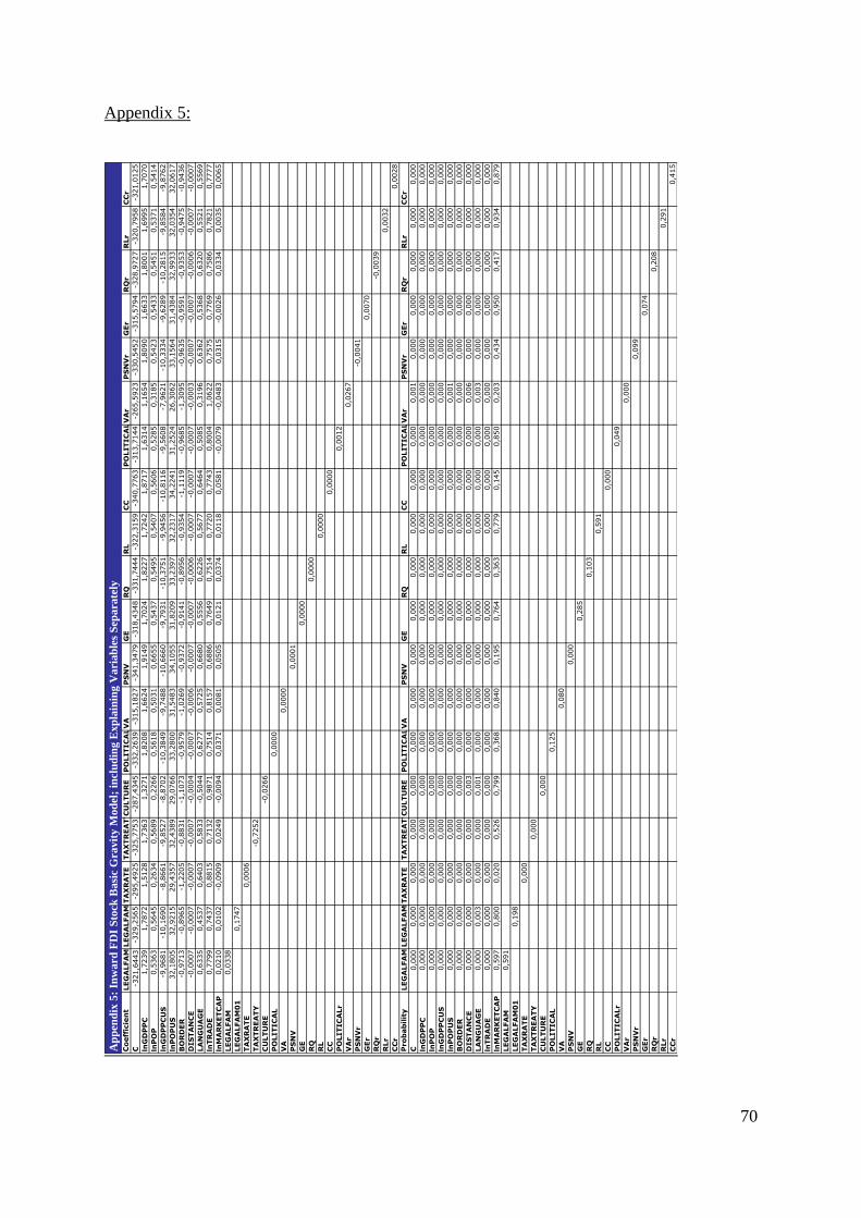
70

Appendix 5:

Ap

pen

dix

5:

Inw

ard

FD

I S

tock

Basi

c G

ravit

y M

od

el;

incl

ud

ing E

xp

lain

ing V

ari

ab

les

Sep

ara

tely

Co

eff

icie

nt

LEG

ALFA

MLEG

ALFA

M0

1TA

XR

ATE

TA

XTR

EA

TYC

ULTU

RE

PO

LITIC

AL

VA

PS

NV

GE

RQ

RL

CC

PO

LITIC

ALrV

Ar

PS

NV

rG

Er

RQ

rR

Lr

CC

r

C-3

21,6

443

-329,2

565

-295,4

925

-325,7

753

-287,4

345

-332,2

639

-315,1

827

-341,3

479

-318,4

348

-331,7

444

-322,3

159

-340,7

763

-313,7

144

-265,5

923

-330,5

452

-315,5

794

-328,9

727

-320,7

958

-321,0

125

lnG

DP

PC

1,7

239

1,7

872

1,5

128

1,7

363

1,3

271

1,8

208

1,6

624

1,9

149

1,7

024

1,8

227

1,7

242

1,8

717

1,6

314

1,1

654

1,8

090

1,6

633

1,8

001

1,6

995

1,7

070

lnP

OP

0,5

363

0,5

645

0,2

634

0,5

689

0,2

266

0,5

618

0,5

031

0,6

655

0,5

437

0,5

495

0,5

407

0,5

606

0,5

285

0,3

185

0,5

423

0,5

433

0,5

451

0,5

371

0,5

414

lnG

DP

PC

US

-9,9

681

-10,1

690

-8,8

661

-9,8

527

-8,8

702

-10,3

849

-9,7

488

-10,6

660

-9,7

931

-10,3

751

-9,9

456

-10,8

116

-9,5

608

-7,9

621

-10,3

334

-9,6

289

-10,2

815

-9,8

584

-9,8

762

lnP

OP

US

32,1

805

32,9

215

29,4

357

32,4

389

29,0

766

33,2

800

31,5

483

34,1

055

31,8

209

33,2

397

32,2

317

34,2

241

31,2

524

26,3

062

33,1

564

31,4

384

32,9

933

32,0

354

32,0

617

BO

RD

ER

-0,9

713

-0,8

965

-1,2

205

-0,8

831

-1,1

073

-0,9

579

-1,0

269

-0,9

372

-0,9

141

-0,8

956

-0,9

354

-1,1

119

-0,9

685

-1,3

095

-0,9

635

-0,9

591

-0,9

353

-0,9

475

-0,9

436

DIS

TA

NC

E-0

,0007

-0,0

007

-0,0

007

-0,0

007

-0,0

004

-0,0

007

-0,0

006

-0,0

007

-0,0

007

-0,0

006

-0,0

007

-0,0

007

-0,0

007

-0,0

003

-0,0

007

-0,0

007

-0,0

006

-0,0

007

-0,0

007

LA

NG

UA

GE

0,6

335

0,4

537

0,6

403

0,5

833

-0,5

044

0,6

277

0,5

725

0,6

680

0,5

556

0,6

226

0,5

677

0,6

464

0,5

085

0,3

196

0,6

362

0,5

368

0,6

320

0,5

521

0,5

569

lnTR

AD

E0,7

799

0,7

437

0,8

815

0,7

132

0,9

871

0,7

514

0,8

157

0,6

886

0,7

649

0,7

514

0,7

720

0,7

743

0,8

004

1,0

622

0,7

575

0,7

769

0,7

586

0,7

821

0,7

777

lnM

AR

KE

TC

AP

0,0

210

0,0

102

-0,0

909

0,0

249

-0,0

094

0,0

371

0,0

081

0,0

505

0,0

121

0,0

374

0,0

118

0,0

581

-0,0

079

-0,0

483

0,0

315

-0,0

026

0,0

334

0,0

035

0,0

065

LEG

ALFA

M0,0

338

LEG

ALFA

M0

10,1

747

TA

XR

ATE

0,0

006

TA

XTR

EA

TY

-0,7

252

CU

LTU

RE

-0,0

266

PO

LITIC

AL

0,0

000

VA

0,0

000

PS

NV

0,0

001

GE

0,0

000

RQ

0,0

000

RL

0,0

000

CC

0,0

000

PO

LITIC

ALr

0,0

012

VA

r0,0

267

PS

NV

r-0

,0041

GEr

0,0

070

RQ

r-0

,0039

RLr

0,0

032

CC

r0,0

028

Pro

bab

ilit

yLEG

ALFA

MLEG

ALFA

M0

1TA

XR

ATE

TA

XTR

EA

TYC

ULTU

RE

PO

LITIC

AL

VA

PS

NV

GE

RQ

RL

CC

PO

LITIC

ALrV

Ar

PS

NV

rG

Er

RQ

rR

Lr

CC

r

C0,0

00

0,0

00

0,0

00

0,0

00

0,0

00

0,0

00

0,0

00

0,0

00

0,0

00

0,0

00

0,0

00

0,0

00

0,0

00

0,0

01

0,0

00

0,0

00

0,0

00

0,0

00

0,0

00

lnG

DP

PC

0,0

00

0,0

00

0,0

00

0,0

00

0,0

00

0,0

00

0,0

00

0,0

00

0,0

00

0,0

00

0,0

00

0,0

00

0,0

00

0,0

00

0,0

00

0,0

00

0,0

00

0,0

00

0,0

00

lnP

OP

0,0

00

0,0

00

0,0

00

0,0

00

0,0

00

0,0

00

0,0

00

0,0

00

0,0

00

0,0

00

0,0

00

0,0

00

0,0

00

0,0

00

0,0

00

0,0

00

0,0

00

0,0

00

0,0

00

lnG

DP

PC

US

0,0

00

0,0

00

0,0

00

0,0

00

0,0

00

0,0

00

0,0

00

0,0

00

0,0

00

0,0

00

0,0

00

0,0

00

0,0

00

0,0

00

0,0

00

0,0

00

0,0

00

0,0

00

0,0

00

lnP

OP

US

0,0

00

0,0

00

0,0

00

0,0

00

0,0

00

0,0

00

0,0

00

0,0

00

0,0

00

0,0

00

0,0

00

0,0

00

0,0

00

0,0

01

0,0

00

0,0

00

0,0

00

0,0

00

0,0

00

BO

RD

ER

0,0

00

0,0

00

0,0

00

0,0

00

0,0

00

0,0

00

0,0

00

0,0

00

0,0

00

0,0

00

0,0

00

0,0

00

0,0

00

0,0

00

0,0

00

0,0

00

0,0

00

0,0

00

0,0

00

DIS

TA

NC

E0,0

00

0,0

00

0,0

00

0,0

00

0,0

03

0,0

00

0,0

00

0,0

00

0,0

00

0,0

00

0,0

00

0,0

00

0,0

00

0,0

06

0,0

00

0,0

00

0,0

00

0,0

00

0,0

00

LA

NG

UA

GE

0,0

00

0,0

03

0,0

00

0,0

00

0,0

01

0,0

00

0,0

00

0,0

00

0,0

00

0,0

00

0,0

00

0,0

00

0,0

00

0,0

03

0,0

00

0,0

00

0,0

00

0,0

00

0,0

00

lnTR

AD

E0,0

00

0,0

00

0,0

00

0,0

00

0,0

00

0,0

00

0,0

00

0,0

00

0,0

00

0,0

00

0,0

00

0,0

00

0,0

00

0,0

00

0,0

00

0,0

00

0,0

00

0,0

00

0,0

00

lnM

AR

KE

TC

AP

0,5

97

0,8

00

0,0

20

0,5

26

0,7

99

0,3

68

0,8

40

0,1

95

0,7

64

0,3

63

0,7

79

0,1

45

0,8

50

0,2

03

0,4

34

0,9

50

0,4

17

0,9

34

0,8

79

LEG

ALFA

M0,5

91

LEG

ALFA

M0

10,1

98

TA

XR

ATE

0,0

00

TA

XTR

EA

TY

0,0

00

CU

LTU

RE

0,0

00

PO

LITIC

AL

0,1

25

VA

0,0

80

PS

NV

0,0

00

GE

0,2

85

RQ

0,1

03

RL

0,5

91

CC

0,0

00

PO

LITIC

ALr

0,0

49

VA

r0,0

00

PS

NV

r0,0

99

GEr

0,0

74

RQ

r0,2

08

RLr

0,2

91

CC

r0,4

15

71

Appendix 6:

Ap

pen

dix

6:

Ou

tward

FD

I S

tock

Basi

c G

ravit

y M

od

el;

incl

ud

ing E

xp

lain

ing

Vari

ab

les

Sep

ara

tely

Co

eff

icie

nt

LEG

ALFA

MLEG

ALFA

M0

1TA

XR

ATE

TA

XTR

EA

TYC

ULTU

RE

PO

LITIC

AL

VA

PS

NV

GE

RQ

RL

CC

PO

LITIC

ALrV

Ar

PS

NV

rG

Er

RQ

rR

Lr

CC

r

C-2

75,5

272

-241,9

889

-267,1

996

-255,2

779

-239,5

959

-268,4

323

-257,7

762

-259,3

711

-280,7

443

-273,6

211

-270,6

357

-264,8

090

-273,1

086

-248,2

234

-265,4

944

-286,7

496

-269,1

348

-270,7

271

-273,3

399

lnG

DP

PC

0,7

119

0,4

104

0,6

123

0,5

657

0,3

681

0,6

506

0,5

400

0,5

585

0,7

272

0,6

992

0,6

717

0,6

097

0,7

032

0,4

362

0,6

174

0,8

257

0,6

589

0,6

871

0,7

157

lnP

OP

0,3

146

0,1

922

0,3

615

0,2

603

0,1

230

0,2

980

0,2

620

0,2

704

0,2

760

0,2

908

0,2

832

0,2

837

0,2

927

0,2

233

0,2

727

0,2

831

0,2

814

0,2

894

0,2

825

lnG

DP

PC

US

-6,8

763

-5,9

442

-6,5

341

-6,3

660

-5,7

054

-6,7

478

-6,3

056

-6,3

622

-7,2

935

-6,9

620

-6,8

946

-6,6

143

-6,9

735

-5,9

476

-6,6

261

-7,6

684

-6,8

067

-6,9

082

-7,0

503

lnP

OP

US

27,1

301

23,8

267

26,1

906

25,1

367

23,6

181

26,4

160

25,3

210

25,4

790

27,7

581

26,9

713

26,6

891

26,0

539

27,0

084

24,3

055

26,1

564

28,6

167

26,5

740

26,7

692

27,0

869

BO

RD

ER

-0,0

174

-0,3

304

-0,0

005

-0,1

585

-0,1

884

-0,1

143

-0,1

397

-0,1

221

-0,2

441

-0,0

058

-0,1

974

-0,1

596

-0,0

915

-0,1

982

-0,1

256

-0,0

782

-0,0

758

-0,1

217

-0,1

405

DIS

TA

NC

E-0

,0002

0,0

000

0,0

000

-0,0

001

0,0

000

-0,0

001

-0,0

001

-0,0

001

0,0

000

-0,0

001

-0,0

001

-0,0

001

-0,0

001

-0,0

001

-0,0

001

0,0

001

-0,0

001

-0,0

001

-0,0

001

LA

NG

UA

GE

0,3

795

1,2

389

0,8

274

0,7

243

0,2

067

0,7

619

0,7

153

0,7

190

0,8

243

0,7

707

0,7

950

0,7

412

0,8

003

0,6

635

0,7

548

0,8

506

0,7

844

0,7

899

0,8

202

lnTR

AD

E0,5

254

0,6

944

0,5

626

0,6

227

0,6

900

0,5

733

0,6

083

0,5

980

0,6

083

0,5

628

0,5

818

0,5

909

0,5

591

0,6

580

0,5

865

0,5

722

0,5

769

0,5

630

0,5

620

lnM

AR

KE

TC

AP

0,1

101

0,1

487

0,0

916

0,1

148

0,1

000

0,1

385

0,1

120

0,1

152

0,1

463

0,1

481

0,1

535

0,1

330

0,1

487

0,0

994

0,1

260

0,1

832

0,1

394

0,1

552

0,1

659

LEG

ALFA

M-0

,2536

LEG

ALFA

M0

1-0

,6878

TA

XR

ATE

-0,0

001

TA

XTR

EA

TY

0,3

149

CU

LTU

RE

-0,0

122

PO

LITIC

AL

0,0

000

VA

0,0

000

PS

NV

0,0

000

GE

0,0

000

RQ

0,0

000

RL

0,0

000

CC

0,0

000

PO

LITIC

ALr

-0,0

015

VA

r0,0

055

PS

NV

r-0

,0035

GEr

-0,0

204

RQ

r-0

,0064

RLr

-0,0

081

CC

r-0

,0103

Pro

bab

ilit

yLEG

ALFA

MLEG

ALFA

M0

1TA

XR

ATE

TA

XTR

EA

TYC

ULTU

RE

PO

LITIC

AL

VA

PS

NV

GE

RQ

RL

CC

PO

LITIC

ALrV

Ar

PS

NV

rG

Er

RQ

rR

Lr

CC

r

C0,0

00

0,0

00

0,0

00

0,0

00

0,0

00

0,0

00

0,0

00

0,0

00

0,0

00

0,0

00

0,0

00

0,0

00

0,0

00

0,0

00

0,0

00

0,0

00

0,0

00

0,0

00

0,0

00

lnG

DP

PC

0,0

00

0,0

00

0,0

00

0,0

00

0,0

00

0,0

00

0,0

00

0,0

00

0,0

00

0,0

00

0,0

00

0,0

00

0,0

00

0,0

00

0,0

00

0,0

00

0,0

00

0,0

00

0,0

00

lnP

OP

0,0

00

0,0

00

0,0

00

0,0

00

0,0

06

0,0

00

0,0

00

0,0

00

0,0

00

0,0

00

0,0

00

0,0

00

0,0

00

0,0

00

0,0

00

0,0

00

0,0

00

0,0

00

0,0

00

lnG

DP

PC

US

0,0

00

0,0

01

0,0

00

0,0

00

0,0

01

0,0

00

0,0

00

0,0

00

0,0

00

0,0

00

0,0

00

0,0

00

0,0

00

0,0

01

0,0

00

0,0

00

0,0

00

0,0

00

0,0

00

lnP

OP

US

0,0

00

0,0

00

0,0

00

0,0

00

0,0

00

0,0

00

0,0

00

0,0

00

0,0

00

0,0

00

0,0

00

0,0

00

0,0

00

0,0

00

0,0

00

0,0

00

0,0

00

0,0

00

0,0

00

BO

RD

ER

0,9

12

0,0

36

0,9

97

0,3

19

0,2

24

0,4

71

0,3

88

0,4

42

0,1

22

0,9

71

0,2

14

0,3

16

0,5

63

0,2

18

0,4

28

0,6

10

0,6

33

0,4

40

0,3

71

DIS

TA

NC

E0,0

53

0,9

87

0,8

44

0,2

17

0,7

94

0,2

17

0,2

01

0,1

75

0,7

73

0,5

64

0,2

87

0,1

37

0,2

74

0,4

76

0,2

13

0,3

80

0,4

62

0,2

89

0,2

57

LA

NG

UA

GE

0,0

00

0,0

00

0,0

00

0,0

00

0,0

61

0,0

00

0,0

00

0,0

00

0,0

00

0,0

00

0,0

00

0,0

00

0,0

00

0,0

00

0,0

00

0,0

00

0,0

00

0,0

00

0,0

00

lnTR

AD

E0,0

00

0,0

00

0,0

00

0,0

00

0,0

00

0,0

00

0,0

00

0,0

00

0,0

00

0,0

00

0,0

00

0,0

00

0,0

00

0,0

00

0,0

00

0,0

00

0,0

00

0,0

00

0,0

00

lnM

AR

KE

TC

AP

0,0

00

0,0

00

0,0

03

0,0

00

0,0

01

0,0

00

0,0

00

0,0

00

0,0

00

0,0

00

0,0

00

0,0

00

0,0

00

0,0

01

0,0

00

0,0

00

0,0

00

0,0

00

0,0

00

LEG

ALFA

M0,0

00

LEG

ALFA

M0

10,0

00

TA

XR

ATE

0,0

18

TA

XTR

EA

TY

0,0

13

CU

LTU

RE

0,0

00

PO

LITIC

AL

0,0

21

VA

0,5

53

PS

NV

0,9

06

GE

0,0

00

RQ

0,0

00

RL

0,0

00

CC

0,0

24

PO

LITIC

ALr

0,0

01

VA

r0,0

08

PS

NV

r0,0

59

GEr

0,0

00

RQ

r0,0

05

RLr

0,0

00

CC

r0,0

00

Documents

The Effect of Cultural and Political Factors on FDI B. 325537 - id...1 The Effect of Cultural and Political Factors on FDI Between the US and Partner Countries Author: B.F.M. Lausberg