The Effect of Concealed Handgun Laws on Crime:Beyond the Dummy Variables*

Hashem DezhbakhshDepartment of Economics

Emory UniversityAtlanta, Ga 30322-2240

Tel. (404) 727-4679Fax (404) 727-4639econhd@emory.edu

and

Paul H. RubinDepartment of Economics

Emory UniversityAtlanta, Ga 30322-2240

Tel. (404) 727-6365Fax (404) 727-4639prubin@emory.edu

January 1999

* We have benefited from comments by Issac Ehrlich, Belton Fleisher, Daniel Nagin, andManoucher Parvin. The usual disclaimer applies, however. We also thank John Lott and DavidMustard for providing us with the data and the Emory University Research Committee for financialsupport.

1

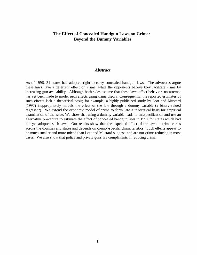
The Effect of Concealed Handgun Laws on Crime:Beyond the Dummy Variables

Abstract

As of 1996, 31 states had adopted right-to-carry concealed handgun laws. The advocates arguethese laws have a deterrent effect on crime, while the opponents believe they facilitate crime byincreasing gun availability. Although both sides assume that these laws affect behavior, no attempthas yet been made to model such effects using crime theory. Consequently, the reported estimates ofsuch effects lack a theoretical basis; for example, a highly publicized study by Lott and Mustard(1997) inappropriately models the effect of the law through a dummy variable (a binary-valuedregressor). We extend the economic model of crime to formulate a theoretical basis for empiricalexamination of the issue. We show that using a dummy variable leads to misspecification and use analternative procedure to estimate the effect of concealed handgun laws in 1992 for states which hadnot yet adopted such laws. Our results show that the expected effect of the law on crime variesacross the counties and states and depends on county-specific characteristics. Such effects appear tobe much smaller and more mixed than Lott and Mustard suggest, and are not crime-reducing in mostcases. We also show that police and private guns are compliments in reducing crime.

2

I. Introduction

The right-to-carry concealed handgun laws--“shall issue” laws--and their possible effects on

crime have been the subject of extensive policy and academic debate as more states adopt such

laws. 1 From 1977 to 1992 ten states passed such laws making it much easier to obtain licenses

to carry concealed handguns, and thirteen states adopted this law between 1992 and 1996.

These laws are at odds with the recently passed Federal Brady Bill, which is restrictive in terms

of gun ownership, reflecting the conflict among various levels of government regarding the role

of handguns in violence. Such conflict also extends to academic circles. Some argue the

concealed handgun laws increase criminals’ access to guns through theft, overpowering victims,

or black market, thus leading to a civil arms race which can only increase crime (Cook (1991),

Kellermann et al. (1995), McDowall, Loftin, and Wiersema (1995), Cook and Ludwig (1996),

Cook and Leitzel (1996), Hemenway (1997), and Ludwig (1998)). We call this outcome the

“facilitating effect” of concealed handgun laws. The supporters of these laws dispute the

facilitating effect, maintaining that the effect is opposite. They argue that allowing citizens to

carry firearms will increase criminals’ uncertainty regarding an armed response, thus leading to

less crime— the “deterrence effect” (Kleck and Patterson (1993), Polsby (1994, 1995), Lott and

Mustard (1997) and Lott (1998)).

No study has formalized the above arguments theoretically. Such a theoretical basis is

necessary for any empirical investigation of the issue. In this paper we formalize these

arguments in the context of the economic model of crime. We demonstrate that the direction

and magnitude of any resulting change would depend on the parameters of the criminal’s

1 Henceforth, we refer to such provisions as "concealed handgun" laws. These laws are also referred to as“shall issue” laws (laws mandating that authorities “shall issue” permits to carry concealed handguns).

3

optimization problem and the characteristics of the individual and his social and economic

setting. This means that any change in crime rate induced by concealed handgun laws will

depend on demographic, social, and economic specifities of the observation units (in this case

counties). Thus, these laws might lead to increases in crime in some jurisdictions and decreases

in others. For example, one would expect the effect of the law on crime to be more pronounced

in more populated counties, because authorities who have discretion over issuing handgun-

carrying permits in absence of a concealed handgun law are the most restrictive in these

counties. The largest changes in handgun density as the result of such laws are therefore

expected in populated counties. Moreover, since the law excludes juveniles from receiving gun-

carrying permits, the deterrent effect is expected to be smaller in counties with a younger

population. Other demographic determinants of propensity to carry a concealed weapon may

lead to similar differential effects.

We also empirically examine the effect of concealed handgun laws on crime. We base our

empirical analysis on the aforementioned theoretical considerations by allowing the effect of the

law on crime to be a function of characteristics of the population in a given jurisdiction. We can

then infer how various factors influence the magnitude of the change in crime resulting from

these laws. More specifically, we project what the 1992 crime rate for counties without such a

law would have been if the county had adopted such a law by 1992. We then compare these

projections, which are a function of county characteristics, with actual crime data for each

county in 1992 to infer how the absence of the law has affected crime in these counties. We

also examine the relationship between these projected changes and county characteristics. We

use Lott and Mustard’s data which covers 3,054 counties for the period 1977-1992 and includes

series on various categories of crime and arrest rates and economic, demographic, and political

4

variables. The rich data set allows us to exploit cross county heterogeneities, while our theory-

based empirical procedure allows us to make state level inference about the potential effect of

the law.

Ignoring specific population characteristics when modeling the effect of the law leads to

model misspecification and invalid inference. For example, in a highly publicized study, which

covers more than 3000 U.S. counties over a decade, Lott and Mustard (1997) use a dummy

variable to model the effect of the law as a shift in the intercept of the linear crime equation they

estimate.2 The method is predicated on two assumptions: (1) all behavioral (response)

parameters of this equation (slope coefficients) are fixed— unaffected by the law and (2) the

effect of the law on crime is identical across counties. We demonstrate that these assumptions

can be rejected both on theoretical and empirical grounds. Our procedure is intended to

overcome such shortcoming.

The remaining sections are organized as follows: Section II elaborates on the stated effects

of the concealed handgun laws and extends the economic model of crime to examine such

effects. Section III discusses the estimation issues involved in measuring the effect of these laws

and the problems with using dummy variables for this purpose. This section also presents an

alternative estimation procedure that draws on the theoretical considerations discussed in

Section II. Section IV describes the data and presents and discusses the results. Section V

contains concluding remarks.

II- Concealed Handgun Laws and The Economic Model of Crime

2 Lott and Mustard report that passage of concealed handgun laws by a state causes a significant reduction inviolent as well as property crime rates (Lott and-Mustard, Table 11). They attribute their results to adeterrent effect.

5

Thirty one states have so far adopted concealed handgun laws.3 These laws require that

permits to carry concealed handguns be granted to any adult applicant unless the individual has

a criminal record or a history of serious mental illness. Prior to adopting these laws, local

authorities had discretion in granting such permits on a case by case basis, and the most

populated counties were the most restrictive in issuing such permits (Lott and Mustard (1997)).

The supporters of concealed handgun laws argue that allowing law-abiding citizens to carry

concealed handguns increases the overall security by deterring attackers (Kleck and Patterson

(1993), Polsby (1995), and Lott and Mustard (1997)). Since the firearms are concealed,

predators do not know a priori which potential victims or bystanders might be armed. The

armed citizens, therefore, not only enhance their own security but also provide a positive

externality for unarmed citizens. The resulting uncertainty increases the criminal’s perceived

failure probability, leading to a lower expected benefit from (or a higher expected cost of) a

criminal act and therefore to a lower crime rate.

The opponents of these laws are skeptical of such implications (Cook (1991), Kellermann

et al. (1993, 1995), Cook, Molliconi, and Cole (1995), McDowall, Loftin, and Wiersema

(1995), Cook and Ludwig (1996), Hemenway (1997), and Ludwig (1998)). They argue, to the

contrary, that these laws are likely to increase the crime rate. For example, Cook and Leitzel

(1996) note that only a small percentage of felons and youths use the primary market to acquire

3 States are adopting these laws at an increasing rate. Only 8 states had adopted such laws by 1986. By1992, another 10 states had adopted them, and since then 13 more states have joined the group.

6

their handguns; the rest rely on friends, theft, or on street transactions to acquire handguns.

Through these channels, concealed handgun laws may increase the number of guns available to

criminals. Criminals can also use their victims’ guns against them, as many individuals who

suddenly find themselves involved in a violent confrontation may not be able to use their guns

effectively (Kellermann et al. (1995)). Overall, these authors believe that increased gun

availability lowers the criminals’ cost of illegally obtaining firearms, thus fueling a civilian arms

race. The enhanced prevalence of guns, in turn, prompts their substitution for less lethal

weapons in hostile confrontations, thus leading to an increase in crime rates (Ludwig (1998)).

The arguments on both sides imply that the net change in expected benefit from committing

crime is the causal link between concealed handgun laws and crime rates. The direction and

magnitude of such change depends on the relative strength of the hypothesized forces. In the

rest of this section we use the economic model of crime to formalize theses arguments, to

examine theoretically the effect of these laws on crime, and to provide a basis for empirical

examination of the issue.

Modeling the Effect of the Law:

The economic models of criminal behavior--Fleisher (1966), Becker (1968), Sjoquist

(1973), Ehrlich (1975), and Block and Heineke (1975)--are formulated within the framework of

the theory of choice under uncertainty. These models derive a supply, or production offense,

function assuming an optimizing agent who allocates time between legal and/or illegal activities

in such a way as to maximize expected utility. Given the empirical focus of this paper, we do

not develop a new crime model; rather, we extend an existing model to incorporate the effect

of the gun laws.

7

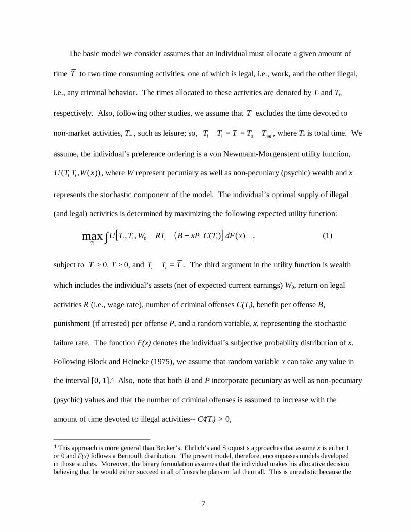
The basic model we consider assumes that an individual must allocate a given amount of

time T to two time consuming activities, one of which is legal, i.e., work, and the other illegal,

i.e., any criminal behavior. The times allocated to these activities are denoted by Tl and Ti,

respectively. Also, following other studies, we assume that T excludes the time devoted to

non-market activities, Tnm, such as leisure; so, T T T T Tl i nm+ = = −0 , where T0 is total time. We

assume, the individual’s preference ordering is a von Newmann-Morgenstern utility function,

U T T W xl i( , ( )), , where W represent pecuniary as well as non-pecuniary (psychic) wealth and x

represents the stochastic component of the model. The individual’s optimal supply of illegal

(and legal) activities is determined by maximizing the following expected utility function:

( )[ ]T

l i l ii

U T T W RT B xP C T dF xmax , , ( ) ( )0 + + −∫ , (1)

subject to Tl ≥ 0, Ti ≥ 0, and T T Tl i+ = . The third argument in the utility function is wealth

which includes the individual’s assets (net of expected current earnings) W0, return on legal

activities R (i.e., wage rate), number of criminal offenses C(Ti), benefit per offense B,

punishment (if arrested) per offense P, and a random variable, x, representing the stochastic

failure rate. The function F(x) denotes the individual’s subjective probability distribution of x.

Following Block and Heineke (1975), we assume that random variable x can take any value in

the interval [0, 1].4 Also, note that both B and P incorporate pecuniary as well as non-pecuniary

(psychic) values and that the number of criminal offenses is assumed to increase with the

amount of time devoted to illegal activities-- C′(Ti) > 0,

4 This approach is more general than Becker’s, Ehrlich’s and Sjoquist’s approaches that assume x is either 1or 0 and F(x) follows a Bernoulli distribution. The present model, therefore, encompasses models developedin those studies. Moreover, the binary formulation assumes that the individual makes his allocative decisionbelieving that he would either succeed in all offenses he plans or fail them all. This is unrealistic because the

8

We introduce concealed handgun laws through an index variable H defined on [0, 1]

interval, where H=0 means no law (no concealed handgun carrying) and a larger H value

indicates a more permissive handgun law. To incorporate the arguments for or against such

laws, we extend the basic model by allowing several of its variables to change with H. Some

changes capture the deterrent effect and others capture the facilitating effect of these laws. The

deterrent effect is rooted in the offender’s concern about an armed response which alters his

perceived probability distribution of the stochastic failure rate x and also increases the possible

punishment for an unsuccessful crime P. We model the probability change by introducing a

parameter, α, that shifts the mean of the perceived distribution--the expected failure rate. This

changes the failure rate to x+αH where the added term αH is zero when H is zero (no law) and

increases with H in such a way that x+αH remains within the [0, 1] range. So, the expected

failure rate in the presence of a concealed handgun law is E(x) + α. The prospect of an armed

response also increases the possible punishment. The perpetrator now, besides fearing financial

sanctions and prison term, must worry about being shot by the victim or a bystander. We model

this by changing P to P(H), where P’(H)>0.

On the other hand, the facilitating effect of the law manifests itself through an increase in the

net benefit per offense B and an increase in the number of offenses, C, given the amount of time

devoted to illegal activities, Ti. Note that B is net of any expense associated with implementing a

crime, so the reduction in the cost of acquiring handguns, which is argued to be the result of

permissive gun laws, increases B. So we change B to B(H), where B’(H)>0. Moreover, the

substitution of handguns for less lethal weapons increases the efficiency of offenses committed

individual may fail on all, none, or a fraction of the attempted offenses; the formulation we adopt allows theindividual to be confronted with a continuum of failure possibilities.

9

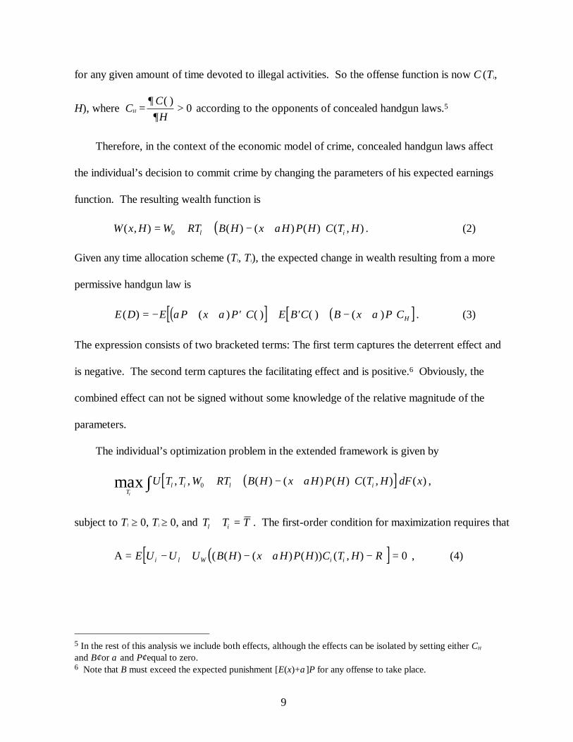
for any given amount of time devoted to illegal activities. So the offense function is now C (Ti,

H), where CH =∂∂CH( )⋅ > 0 according to the opponents of concealed handgun laws.5

Therefore, in the context of the economic model of crime, concealed handgun laws affect

the individual’s decision to commit crime by changing the parameters of his expected earnings

function. The resulting wealth function is

( )W x H W RT B H x H P H C T Hl i( , ) ( ) ( ) ( ) ( , )= + + − +0 α . (2)

Given any time allocation scheme (Tl, Ti), the expected change in wealth resulting from a more

permissive handgun law is

( )[ ] ( )[ ]E D E P x P C E B C B x P CH( ) ( ) ( ) ( ) ( )= − + + ′ ⋅ + ′ ⋅ + − +α α α . (3)

The expression consists of two bracketed terms: The first term captures the deterrent effect and

is negative. The second term captures the facilitating effect and is positive.6 Obviously, the

combined effect can not be signed without some knowledge of the relative magnitude of the

parameters.

The individual’s optimization problem in the extended framework is given by

( )[ ]T

l i l ii

U T T W RT B H x H P H C T H dF xmax , , ( ) ( ) ( ) ( , ) ( )0 + + − +∫ α ,

subject to Tl ≥ 0, Ti ≥ 0, and T T Tl i+ = . The first-order condition for maximization requires that

( )[ ]Α = − + − + − =E U U U B H x H P H C T H Ri l W i i( ( ) ( ) ( )) ( , )α 0 , (4)

5 In the rest of this analysis we include both effects, although the effects can be isolated by setting either CH

and B′ or α and P′ equal to zero.6 Note that B must exceed the expected punishment [E(x)+α]P for any offense to take place.

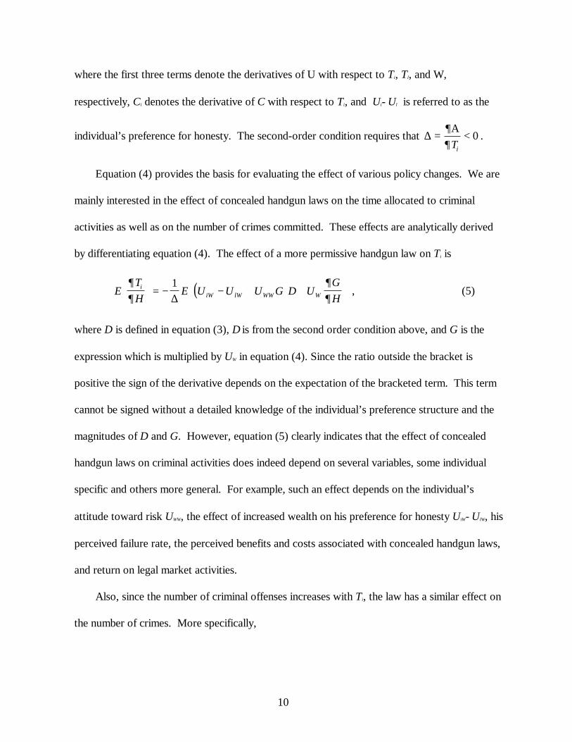
10

where the first three terms denote the derivatives of U with respect to Ti, Tl, and W,

respectively, Ci denotes the derivative of C with respect to Ti, and Ui− Ul is referred to as the

individual’s preference for honesty. The second-order condition requires that ∆ Α= <∂∂Ti

0 .

Equation (4) provides the basis for evaluating the effect of various policy changes. We are

mainly interested in the effect of concealed handgun laws on the time allocated to criminal

activities as well as on the number of crimes committed. These effects are analytically derived

by differentiating equation (4). The effect of a more permissive handgun law on Ti is

( )ETH

E U U U G D UGH

iiW lW WW W

∂∂

∂∂

= − − + +

1∆ , (5)

where D is defined in equation (3), ∆ is from the second order condition above, and G is the

expression which is multiplied by UW in equation (4). Since the ratio outside the bracket is

positive the sign of the derivative depends on the expectation of the bracketed term. This term

cannot be signed without a detailed knowledge of the individual’s preference structure and the

magnitudes of D and G. However, equation (5) clearly indicates that the effect of concealed

handgun laws on criminal activities does indeed depend on several variables, some individual

specific and others more general. For example, such an effect depends on the individual’s

attitude toward risk UWW, the effect of increased wealth on his preference for honesty UiW− UlW, his

perceived failure rate, the perceived benefits and costs associated with concealed handgun laws,

and return on legal market activities.

Also, since the number of criminal offenses increases with Ti, the law has a similar effect on

the number of crimes. More specifically,

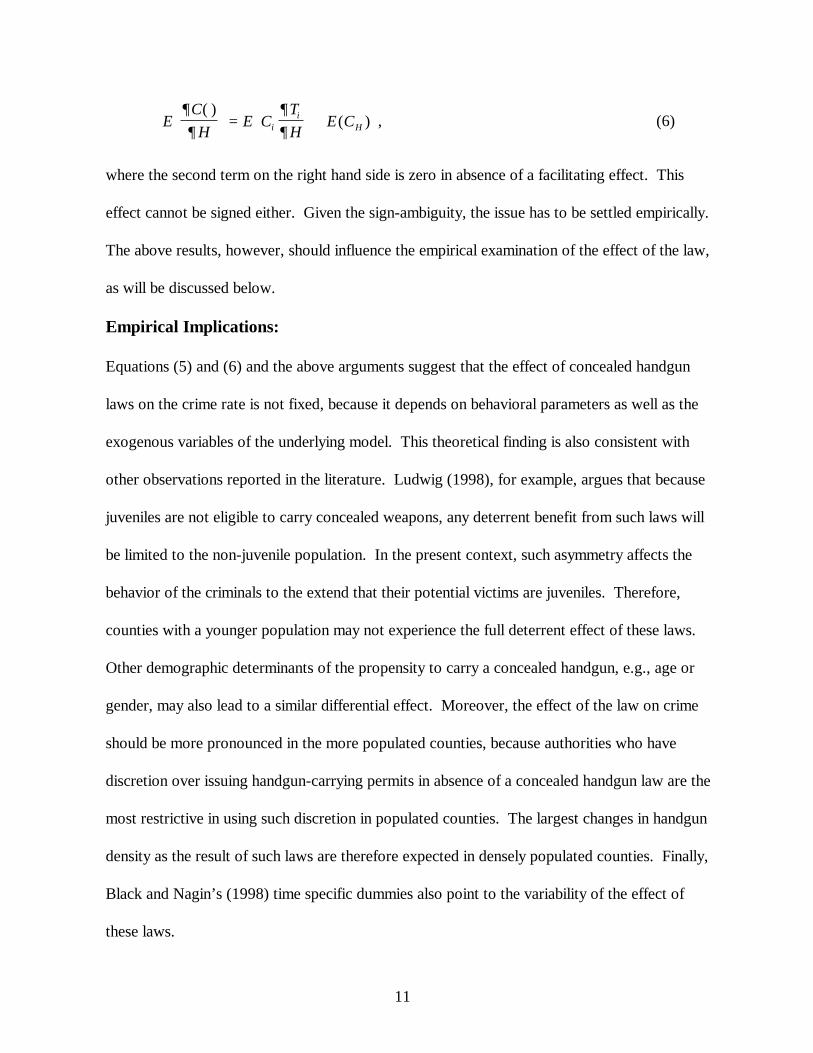
11

ECH

E CTH

E Cii

H

∂∂

∂∂

( )( )

⋅

=

+ , (6)

where the second term on the right hand side is zero in absence of a facilitating effect. This

effect cannot be signed either. Given the sign-ambiguity, the issue has to be settled empirically.

The above results, however, should influence the empirical examination of the effect of the law,

as will be discussed below.

Empirical Implications:

Equations (5) and (6) and the above arguments suggest that the effect of concealed handgun

laws on the crime rate is not fixed, because it depends on behavioral parameters as well as the

exogenous variables of the underlying model. This theoretical finding is also consistent with

other observations reported in the literature. Ludwig (1998), for example, argues that because

juveniles are not eligible to carry concealed weapons, any deterrent benefit from such laws will

be limited to the non-juvenile population. In the present context, such asymmetry affects the

behavior of the criminals to the extend that their potential victims are juveniles. Therefore,

counties with a younger population may not experience the full deterrent effect of these laws.

Other demographic determinants of the propensity to carry a concealed handgun, e.g., age or

gender, may also lead to a similar differential effect. Moreover, the effect of the law on crime

should be more pronounced in the more populated counties, because authorities who have

discretion over issuing handgun-carrying permits in absence of a concealed handgun law are the

most restrictive in using such discretion in populated counties. The largest changes in handgun

density as the result of such laws are therefore expected in densely populated counties. Finally,

Black and Nagin’s (1998) time specific dummies also point to the variability of the effect of

these laws.

12

Using the county as the basis for aggregation, behavioral equations (5) and (6) can be

written in the following general form:

[ ]ECH

EK W R B P C T x g Ujt

jt jt jt jt jt i jt jt jt

∂∂ α η( )

, , , , ( ), , ( ),⋅

= 0 , (7)

where j and t denote county and time, K[.] is a general function, g(U) is a function denoting

higher derivatives of the utility function, and η is a portmanteau variable capturing influences

which are unaccounted for as well as higher derivatives of the terms included in the above

expression.

The heterogeneity indicated by the above equations has important implications for testing

the effect of concealed handgun laws on crime. In particular the effect is not fixed and should

be allowed to vary across observation units, e.g., counties. Moreover, if the law affects the

behavior of criminals or of citizens, then the testing procedure should allow the behavioral

(response) parameters of the model to change. It seems highly unlikely that the magnitude of the

effects such laws may have on crime rates in a county would be independent of its economic and

demographic characteristics. In fact, the effect may vary with the age and gender composition

of the population, population density, characteristics of police, and economic conditions of the

counties, among other things. Finally, variations across counties within a state in terms of how

easily permits were issued prior to adoption of concealed handgun laws make it necessary to

allow the effect of these laws to be heterogeneous across counties. For example, the most

pronounced changes are expected in counties with the most restrictive licensing practice prior to

the enactment of the law. Ignoring such heterogeneity and assuming that ECH

jt

∂∂

( )⋅

is a fixed

13

quantity leads to estimation bias due to imposing incorrect restriction. We later report empirical

evidence to support this point.

Also, note that a crime equation in implicit form can be derived from the first order

condition, equation (4). The right hand side variables and parameters of this equation are the

same as the variables and parameters that appear on the right hand side of equation (7) which

captures the effect of the concealed handgun law on crime. We maintain the same parallel

between our crime equation and the equation we propose for measuring the effect of the law.

III- Estimation Methods and Issues

In regression analysis an intercept-shifting dummy variable is often used to estimate the

effect of an institutional change. The statistical and conceptual ramifications of this practice is

seldom examined, particularly when the empirical analysis is not predicated on economic

theory. To better motivate our procedure which is intended to overcome the shortcomings of

this approach, we elaborate on this issue using Lott and Mustard’s (1997) highly publicized

study on the effect of concealed handgun laws on crime.7 Lott and Mustard use county level

panel data to estimate several linear crime equations. The dependent variable in each equation

is one of several crime rates— murder, rape, aggravated assault, robbery, burglary, larceny, and

auto theft. The regressors include the arrest rate corresponding to that crime category, a host

of economic and socio-demographic factors, and a binary variable measuring the status of the

concealed handgun law. This variable equals 1 if a county has such a law in place in a given

7 Lott and Mustard use the most comprehensive data set to examine this issue. There are several other usefulbut smaller studies that examine the effect of gun availability on crime; See Kleck (1995) and Lott andMustard (1997) for a review.

14

period and 0 otherwise. The other regressors serve as control variables. The model they

estimate is therefore

C H A Xjt jt jt jt jt= + + + +α γ β δ ε , (8)

where H is the binary variable, A is the arrest rate, X includes the economic and demographic

variables and a set of time and county dummies (one for each sampling year or county), ε is the

regression error, and j and t denote counties and time periods, respectively.

Lott and Mustard's inference about the effect of concealed handgun laws on various

categories of crime is based on the sign and statistical significance of the estimated coefficient

of the binary variable— estimate of γ. A positive and significant estimate suggests that

concealed handgun provisions would increase the crime rate, while a negative and significant

estimate points to the contrary conclusion. Note that they use γ in place of the expression in

the right hand side of equation (7). This expression clearly depends on county specific

exogenous variables as well as the behavioral parameters of the model. Ignoring the

heterogeneity of the effect of the law on various counties and parameterizing the effect as a

fixed parameter leads to biased estimation. The 2SLS estimate of γ reported by Lott and

Mustard is negative, substantially large, and significant for all crime categories, further

15

supporting their deterrence hypothesis.8 The aforementioned bias can perhaps explain these

unusually large negative estimates.9

Following our theoretical results, we allow all behavioral parameters of the regression

model to change with the law, and thus the effect of the law on crime rates to be

heterogeneous across counties. The data will then show which of these parameters the law

indeed affects. We implement this parameter flexibility by first estimating two separate crime

equations, one for counties in states with a concealed handgun law and the other for the

remaining counties:

C A Xl jt l l l jt l l jt l jt, , , , ,= + + +α β δ ε (9a)

C A Xnl jt nl nl nl jt nl nl jt nl jt, , , , ,= + + +α β δ ε (9b)

where l, nl indicate the presence or the absence of the concealed handgun law, respectively.

Then, we examine whether the law affects the response parameters by using an asymptotic

Wald test of the null hypothesis H l nl0:Θ Θ= against the alternative H l nl0:Θ Θ≠ , where Θ

denotes ( β δ, ).10 This hypothesis implies that the effect of the law on crime is a constant

parameter γ (or αl− αnl) which does not change across county or over time. This of course is at

8 The 2SLS that treats the arrest rate as an endogenous variable which is itself affected by the crime rate isthe appropriate method for estimating equation (8). In addition to 2SLS, Lott and Mustard use OLS method,which ignores the simultaneity between crime and arrest, to project the expected reduction in the number ofmurders, rapes, robberies, and aggravated assaults for 1992 through 1995 if those states without right-to-carryconcealed handgun provisions had adopted them in 1992. Much of the public attention that Lott and Mustardhave received centers on these OLS based projections and not the more appropriate 2SLS results; see, e.g., thearticle by Richard Morin, in The Washington Post, Sunday, March 23 1997, page 5; also, see Ludwig (1998)and Black and Nagin (1998) who criticize Lott and Mustard on methodological grounds. These authors allfocus on the inappropriate OLS results rather than the 2SLS results.9 Such specification bias also makes the coefficient estimates fragile with respect to small change in themodel such as inclusion or exclusion of various control variables. Bartley, Cohen and Froeb (1998) use themethod suggested by Leamer (1983) to examine the range of estimates of the coefficient of the binary variablein Lott-Mustard specification and find it to be quite wide in many cases.

16

odds with equation (7). A rejection of the null implies that the law affects the response (slope)

parameters of the model, thus rejecting a simple intercept change formulation. As we report in

the next section the null of a fixed parameter effect of the law is rejected strongly in all cases,

making the use of a less restrictive procedure necessary.

We estimate for each county the direction and extent of the change in crime rate that may

result from introducing the concealed handgun law. We determine how different the crime rate

would have been during 1992 in the counties that did not have the concealed handgun law in

place, had they adopted the law by 1992. We obtain these estimates, which are useful for

policy purposes, simply by switching the estimates of the behavioral parameters in equations

(9a) and (9b) and computing the resulting predicted values for the dependent variable (the

crime rate) over the relevant year. The estimates are obtained from ∃ ∃ ∃,C Zj l l nl j92 92= +α Θ ,

where Znl denotes the regressors in equation (9b), Θ denotes ( β δ, ), 92 is year, and j is

restricted to the aforementioned group of counties. These are simply predicted crime rate

conditional on adopting the concealed handgun law. The difference between the predicted and

actual crime rates measures the effect of concealed handgun laws on crime. We emphasize that

our interest is in making an inference about the expected 1992 crime rates conditional on the

law being in place in a county that did not have it in 1992. This estimate is then compared with

the county’s actual 1992 crime rates to estimate the expected change. It is important to note

that in the above comparison, one should not use the county’s predicted crime rate without the

law in 1992, ∃ ∃,αnl nl nl jZ+ Θ 92 , instead of the observed (actual) crime rate Cnl. This is because the

10 The Wald statistic is the quadratic form constructed on the estimate of the difference (Θ l− Θ nl). Thestatistic is asymptotically distributed as a χ2 variate with degrees of freedom equal to the number ofparameters tested (Godfrey (1988, ch. 4) and Lo and Newey (1985), see also Pesaran et al. (1985)).

17

former does not have any information that is useful for our inference but is not contained in the

county’s observed 1992 crime rate. Therefore, if we used the predicted crime rate instead of

the actual crime rate, we would just be adding extra noise (residual), thus reducing the

accuracy of the inference. Also, note that all the information relevant to adopting the law is

incorporated in ∃Θ l which is estimated using counties with the law.

To see how our procedure relates to the theoretical equation (7) and also to formally

contrast this procedure with the intercept-shifting dummy variable approach, consider the

following. The latter parameterizes the law-induced crime change as αl − αnl which is γ in

equation (8)— the shift in the intercept. This parameter is fixed across all counties and

independent of county characteristics. It also implies that the law does not affect any of the

behavioral parameters of the model. We, on the other hand, parameterize the change as

(αl + Θ l Z nl,j92) − Cnl,j92

which after substitution from (9b) and setting the random error ε nl to zero--its expected value-

-yields

(αl − αnl) + (Θ l − Θ nl)Z nl,j92.

Note that the first term in the above expression is the intercept change, used, e.g., by Lott and

Mustard, while the second term is our addition which varies with county characteristics and is a

function of model parameters. This expression is the empirical counterpart of the law-induced

crime change as given by equation (7). Also, note the similarities between the parameters and

variables in this expression and those in the crime equations (9a,b). We documented a similar

parallel between the theoretical counterparts of crime and the change in crime.

We summarize the predictions we so obtain to generate an inference about the potential

influence of the law in each state which did not have a concealed handgun law in 1992. The

18

predictions are further analyzed to determine factors that influence their direction or

magnitude. This approach allows the effect of permissive handgun laws to vary with

population density, racial and gender characteristics, income, and so forth. At the same time, it

exploits the variation in the timing of these state laws to investigate their impact.

Following Ehrlich (1973), in all our estimation we treat the arrest rate, A, as an

endogenous variable that is affected by such variables as lagged crime rate, economic and

demographic variables in the crime equation, police employment and payroll, and a set of

variables to control for political influences. These latter variables include percentage of votes

received by the Republican presidential candidate, and the percentage of a states’ population

that are members of the National Rifle Association.11 We estimate equations (9a) and (9b)

along with the corresponding arrest equations via 2SLS, allowing the concealed handgun law

to also shift the coefficients of the arrest equation in the first stage of estimation; such shifts are

incorporated in cases where the Wald test applied to an arrest equation suggested such a

change is warranted. This ensures the consistency of the second stage estimates. In all our

estimations, we correct the residuals from the second stage least square to account for using

predicted arrest rather than the actual arrest rate in estimation of crime equation; see, e.g.,

Davidson and MacKinnon (1993, ch. 7).

IV- Data and Results12

We use the data provided to us by Lott and Mustard. The data set covers 3,054 counties

for the period 1977-1992. However, since several series are only reported for 1982 through

1992, the effective time span is shorter. The data set includes the FBI’s crime data for murder,

11 See, also, Lott and Mustard (1997), page 42.

19

rape, aggravated assault, and robbery which comprise “violent crime” and auto theft, burglary,

and larceny which comprise “property crime”. The series also include the corresponding arrest

rate for these nine crime categories, population, population density, real per capita personal

income, real per capita unemployment insurance payments, real per capita income maintenance

payments, real per capita retirement payments per person over 65 years of age, and population

characteristics for thirty-six age and race segments (black, white and other; male and female;

and age divisions.) The data set also includes state level data on police employment and

payroll, percentage of votes received by the Republican presidential candidate, and the

percentage of each state’s population that are members of the National Rifle Association. This

is the most exhaustive panel data set available for research in this area.

As indicated earlier, our empirical strategy starts with testing whether the data supports

modeling the effect of the law through an intercept-shifting dummy variable— the hypothesis

of no slope change due to the law. Using an asymptotic Wald test for all nine categories of

crimes, we find that this hypothesis is rejected strongly for all categories of crime. The

statistics for various crime equations are 131.2 (murder), 152.5 (rape), 395.3 (aggravated

assault), 194.2 (robbery), 451.2 (burglary), 323.7 (larceny), 479.3 (auto theft); all statistics

have p-values which are close to zero. That is, in all cases, there are significant changes in

the slope coefficients, so that assuming all changes to be embedded in the intercept is

incorrect. This suggests that the Lott-Mustard results are biased by misspecification. Similar

results for the arrest equation, used in the first stage of the 2SLS estimation, indicate the

coefficients of these equations also change with the law. In fact, we incorporate these

changes when obtaining the predicted arrest rates. A comparison of our predicted arrest

12 We reported some of the empirical results in Dezhbakhsh and Rubin (1998).

20

rates to that of Lott and Mustard’s reveal the inaccuracy introduced by limiting the change to

the intercept term. For example, depending on the crime category, the mean square error of

Lott and Mustard’s predicted arrest rates is from 1.5 to 5.2 times larger than ours. Their

predicted arrest rates also include a large number of negative values (i.e., over 19,000 of

about 33,000 observation for auto theft are negative; the number of negative arrest rates for

aggravated assault and property crimes are, respectively, 9,900 and 13,500.

We use the two stage procedure described earlier to estimate the hypothetical effect on

crime in each county in states that did not have a concealed handgun law in place if such a

law had been in effect in 1992. We examine these effects in two ways, both on a county-by-

county basis. First, we examine for each crime and for each county the predicted effect of

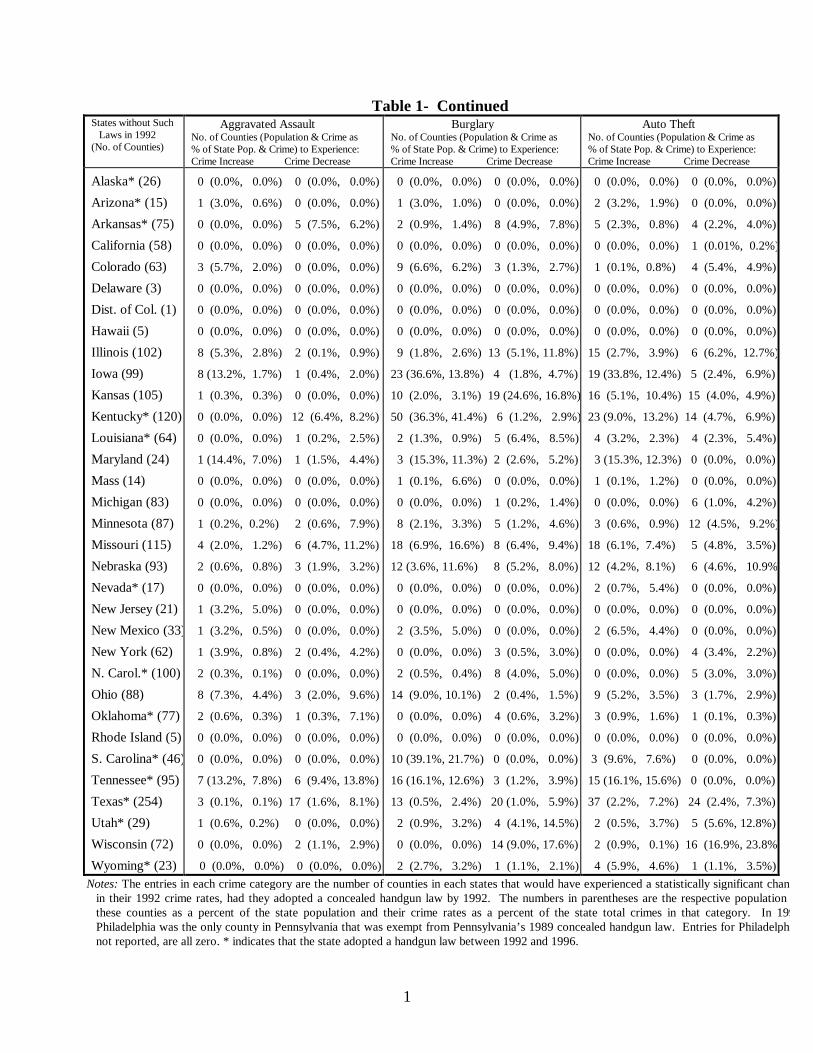
changing the law. Table 1 contains summary statistics derived from these county level

conditional predictions. Second, we examine the effect of county characteristics on predicted

change in crime rates for each aggregated crime category (violent, property). Table 2 reports

results of regressing these predictions on various county characteristics.

The interpretation of Table 1 is as follows: There were thirty-three states without such

laws in 1992, excluding Pennsylvania where Philadelphia county was given exemption from

the law passed in 1989. Consider, for example, murder in Texas. Since Texas is in our

sample, this indicates that in 1992 this state did not have a concealed handgun law in place,

although the * indicates that it had adopted such a law by 1996. There are 254 counties in

Texas as shown in (column 1). Had the concealed handgun law been in effect in Texas in

1992, then in seven of those counties, which include .4% of the population in the state and

account for 9.4% of the state murders, murder rates would have decreased by a statistically

21

significant amount.13 Thus, for counties in six states a concealed handgun law would have

reduced murder rates and for all counties in the other twenty seven states it would have been

ineffective. Overall, the results indicate a relatively small, and crime reducing, effect of

concealed handgun laws on murder rates.

It appears that there would have been little effect on rape with twenty-one states

unaffected, four states with unambiguous increases, and two states with unambiguous

decreases. The effect on robbery would have been an increase in crime for many states. For

counties in thirteen states, there would have been an unambiguous increase in robbery; there

would have been mixed effect (increase in some counties and decrease in some) in counties in

only three states. The overall increase in robbery is not surprising given that concealed

handguns add little deterrence in this case. Many potential robbery targets such as banks and

various shops already have armed protection; therefore, concealed firearm laws do not

provide them with deterrence benefits, but these laws apparently have a large crime

facilitating effect for robbers.

For aggravated assault eleven states would have been unaffected, seven states adversely

affected, and four states would have observed a drop in crime. The result for the remaining

states is mixed. For the three categories of property crime (only two reported in the table)

the effect would have been more mixed. Altogether there were 33 states containing 2074

counties that did not have shall issue laws in 1992, so the largest percentage of counties

predicted to be affected in one direction by changing the law would have been the 15% of

13 If the actual 1992 crime rate for a county falls short of (exceeds) the confidence interval for the projectedcrime rate conditional on the law being in place, then we infer that the law would have increased (decreased)the crime rate for that county.

22

counties predicted to experience an increase in larceny; all other predicted percentage

changes in any direction are less than 10%.

We can also derive policy implications from these ex post predictions for particular states

which had not adopted the law by 1996 (states without an identifying *). Maryland would

expect increases in robbery, assault, burglary, and auto theft, and so probably should not

adopt the law. Similarly New Mexico would expect small increases in robbery and all three

categories of property crime, and so also should not adopt the law. In Iowa, rape, robbery,

assault, burglary and auto theft would increase, if the law is adopted. On the other hand, were

Illinois to adopt a handgun law, then we would expect decreases in murder, robbery,

burglary, and auto theft, but an increase in assault. Kansas could expect reductions in

murder, rape, and burglary, and increases in auto theft and a small increase in assault.

Minnesota might also benefit from the law. For most other states that had not adopted the

law by 1996, effects would be small and mixed.

We next determine which characteristics of counties are associated with increases or decreases

in each aggregate type of crime (violent and property crime). We do this by regressing the

predicted change in crime rates for each of the counties without the law in 1992 on a set of

demographic and economic variables for the county. The economic variables, all measured per

capita, are personal income, unemployment insurance, and retirement payments per person over 65.

We also include (predicted) arrest rates, population density, and demographic variables. Since most

crime is committed by young males, we include number of black and non-black males 10-29 years

old, and similarly for females. We include persons 65 and over, who are perhaps more likely to be

victims than perpetrators of crimes. Finally, we include per capita measures of the number of NRA

members in the state, and police payroll. In all cases, we measure the effect of the relevant variable

23

on predicted changes in crime by category of the existence of a concealed handgun law in the

county.

Regression results, summarized in Table 2. For example, the + marks for arrest rate suggest

that for counties with higher arrest rates, passage of shall issue laws leads to increased crime,

perhaps because residents of such counties have a higher propensity to commit crime which leads to

a larger facilitating effect of handguns. On the other hand, for counties that spend relatively more

on police the laws lead to crime reductions. This is plausible: Higher spending on police will not

effect the deterrent benefit of handguns, but will reduce the facilitating effect of handguns that

benefits criminal activity. It may also be that higher police expenditures enable more effective

screening of would-be gun carriers. This implies that states contemplating passage of handgun laws

should increase expenditure on enforcement; police and private guns seem to be compliments in

crime reduction, not substitutes.

The other consistent results are for likely victims: more elderly people and more young (10-29

year old) non-black females are associated with reduced crime as a result of passage of gun laws.

This may represent evidence of the deterrent effect in some cases, with these variables contributing

to such an effect. Experiments with other specifications indicates that this specification provides

most of the useful information in the data, and is sufficiently aggregated so that the results are easily

interpreted.

V- Concluding Remarks

The role of handguns in violent crimes is a hotly debated public policy issue. Recently many

states have adopted right-to-carry concealed handgun laws. The advocates argue these permissive

24

laws have a deterrent effect on crime, while the opponents point to their potential crime-facilitating

effects through increased gun availability. These arguments imply that concealed handgun laws may

cause a change in the behavior of criminals either directly or as the result of a change in the behavior

of their potential victims. No attempt has yet been made to model the effect of such laws in the

context of the economic theory of crime. The ensuing empirical work, therefore, uses methods that

are not based on the behavioral implications of such laws, although such a theoretical basis is

necessary for any credible examination of the issue. For example, the highly publicized Lott and

Mustard (1997) study that suggests these laws have a strong crime-reducing effect estimates such

effects through a regression dummy variable. This method assumes that the effect of the law on

crime is identical across all counties and independent of any county characteristics, an assumption

flatly contradicted by “conventional wisdom” and by the theory presented in this paper. Research

purporting to demonstrate statistically that handgun related laws have important impacts on crime

rates are of direct relevance to policy debates as well as to legislation. It is imperative that such

debates and subsequent legislation rely on solid empirical findings.

In this paper we extend the economic model of crime to incorporate the effect of concealed

handgun laws. We demonstrate that the direction and magnitude of any resulting change would

depend on the parameters of the criminal’s optimization problem and thus the characteristics of the

individual and his (her) social and economic setting. This means that any change in crime rate

induced by concealed handgun laws will depend on demographic, social, and economic specifities of

the observation units. So these laws might lead to increases in crime in some jurisdictions and

decreases in others.

We then propose an empirical procedure to examine the effect of concealed handgun laws on

crime rates. Our procedure draws on the theoretical considerations resulting from the extended

25

crime model, therefore allowing us to assess the full implications of the right-to-carry gun provisions.

We find that the results of concealed weapons laws are much smaller than suggested by Lott and

Mustard and by no means crime-reducing across all categories. For murder, for example, there is

only a small reduction. For robbery, many states experience increases in crime. For other crimes,

results are ambiguous, with some states showing predicted increases and some predicted decreases.

We identify states (Illinois, Kansas, Minnesota) that might benefit from passage of these laws, and

states (Maryland, New Mexico, and Iowa) that probably would not.

We also examine demographic and other influences on the likely effect of passage of laws on

crime rates. We find that there are predictable patterns on the effect of shall issue laws on crime.

For example, counties spending more on police could expect a decrease in crime from the passage

of a law, or smaller increases where the law leads to an increase in crime; police and private guns

seem to be compliments in crime reduction. Our theoretical and subsequent empirical work points

to the inadequacy of testing the effect of concealed handgun laws without considering their

theoretical implication. The sort of analysis developed here could be used to enable policy makers

to more carefully tailor laws to particular conditions in a jurisdiction.

26

References

Bartley, William Alan and Mark A. Cohen, “The Effect of Concealed Weapon Laws: An Extreme

Bounds Analysis,” Economic Inquiry, 36, April 1998, pp. 258-265.

Becker, Gary S., “Crime and Punishment: An Economic Approach,” Journal of Political Economy,

76(2), 1968, 169-217.

Black, Dan A. and Daniel S. Nagin, Do Right-to-Carry Laws Deter Violent Crime?” Journal of

Legal Studies, 27, January 1998, 209-219.

Block, M.K. and J.M. Heineke, “A Labor Theoretic Analysis of the Criminal Choice,” American

Economic Review, 65(3), June 1975, pp. 314-325.

Cook, Philip J., “The Technology of Personal Violence,” In Tonry M., ed. Crime and Justice: A

Review of Research, University of Chicago Press, 14, 1991, pp. 1-70.

Cook, Philip J. Stephanie Molliconi and Thomas B. Cole, “Regulating Gun Markets,” Journal of

Criminal Law and Criminology, 86(1), Fall 1995, pp. 59-92.

Cook, Philip J. and James A. Leitzel, “Perversity, Futility, Jeopardy: An Economic Analysis of the

Attack on Gun Control,” Law and Contemporary Problems, 59 (1), Winter 1996, pp. 1-28.

Cook, Philip J. and Jen Ludwig, “Guns in America: Results of a Comprehensive National Survey on

Firearms Ownership and Uses,” Report Prepared for National Institute of Justice, 1996.

Davidson, Russell, and James G. MacKinnon, Estimation and Inference in Econometrics, New

York: Oxford University Press, 1993.

Dezhbakhsh, Hashem and Paul H. Rubin, “Lives Saved or Lives Lost: The Effects of Concealed

Handgun Laws on Crime,” American Economic Review, 88(2), May 1998, pp. 468-474.

Ehrlich, Isaac, “Participation in Illegitimate Activities: A Theoretical and Empirical Investigation,”

Journal of Political Economy, 81(3), May-June 1973, pp. 521-565.

Fleisher, Belton, The Economics of Delinquency, Chicago: Univeristy of Chicago Press, 1966.

Godfrey, L.G., Misspecification Tests in Econometrics, The Lagrange Multiplier Principle and

Other Approaches, Cambridge: Cambridge University Press, 1988.

27

Hemenway David, “Survey research and self-defense gun use: An explanation of extreme

overestimates,” Journal of Criminal Law and Criminology, 87, August 1997, pp. 1430-1445.

Kellermann, Arthur L., Fredrick P. Rivara, Norman B. Rushforth, Joyce G. Banton, Donald T.

Reay, Jerry T. Francisco, Ana B. Locci, Janice Prodzinski, Bella B. Hackman, and Grant Somes,

"Gun Ownership as a Risk Factor for Homicide in the Home, "The New England Journal of

Medicine, 329(15), 1993, pp. 1084-1091.

Kellermann, Arthur L., Lori Westohal, Lauri Fischer, and Beverly Harvard, "Weapon Involvement

in Home Invasion Crime," The Journal of the American Medical Association, 273(22), 1995,

pp. 1759-1762.

Kleck, Gary and E. Britt Patterson, “The Impact of Gun Control and Gun Ownership Levels on

Violence Rates,” Journal of Quantitative Criminology, 9, 1993, pp. 249-287.

Kleck, Gary, “Guns and Violence: An Interpretive Review of the Field,” Social Pathology, 1,

January 1995, pp. 12-47.

Leamer, Edward E. and Leonard Herman, "Reporting the Fragility of Regression Estimates," The

Review of Economics and Statistics, 65(2), 1983, pp. 306-317.

Lo, Andrew W. and Whitney K. Newey, “A Large-Sample Chow Test for the Linear Simultaneous

Equation,” Economics Letters, 1985, 18(4), pp. 351-353.

Lott, John R., More Guns, Less Crime: Understanding Crime and Gun-Control Laws, Chicago:

University of Chicago Press, 1998.

Lott, John R. and David B. Mustard, "Crime, Deterrence and Right-to-Carry Concealed

Handguns," Journal of Legal Studies, 26(1), January 1997, pp. 1-68.

Ludwig, Jens, “Concealed-Gun-Carrying Laws and Violent Crime: Evidence from State Panel

Data” International Review of Law and Economics, Forthcoming 1998.

McDowall, David, Colin Loftin, and Brian Wiersema, “Easing Concealed Firearms Laws: Effects on

Homicide in Three States,” Journal of Criminal Law and Criminology, 86(1), Fall 1995, pp.

193-206.

28

Pesaran, M.H., R.P. Smith, and J,S. Yeo, “Testing for Structural Stability and Predictive Failure: A

Review,” Manchester Review, 53, 1985, pp. 280-295.

Polsby, Daniel D., “Firearm Costs, Firearm Benefits and the Limits of Knowledge,” Journal of

Criminal Law and Criminology, 86(1), Fall 1995, pp. 207-220.

______________ , “The False Promise of Gun Control,” Atlantic Monthly, March 1994, pp. 57-70.

Sjoquist, David L., “Property Crime and Economic Behavior: Some Empirical Results, American

Economic Review, 63(3), 1973, pp. 439-446.

Table 1- The Predicted Effect of Adopting Concealed Handgun Laws on Crimes in States without Such Laws in 1992

States without Such Laws in 1992(No. of Counties)

MurderNo. of Counties (Population & Crime as% of State Pop. & Crime) to Experience:Crime Increase Crime Decrease

RapeNo. of Counties (Population & Crime as% of State Pop. & Crime) to Experience:Crime Increase Crime Decrease

RobberyNo. of Counties (Population & Crime as% of State Pop. & Crime) to Experience:Crime Increase Crime Decrease

Alaska* (26)

Arizona* (15)

Arkansas* (75)

California (58)

Colorado (63)

Delaware (3)

Dist. of Col. (1)

Hawaii (5)

Illinois (102)

Iowa (99)

Kansas (105)

Kentucky* (120)

Louisiana* (64)

Maryland (24)

Mass. (14)

Michigan (83)

Minnesota (87)

Missouri (115)

Nebraska (93)

Nevada* (17)

New Jersey (21)

New Mexico (33)

New York (62)

N. Carol.* (100)

Ohio (88)

Oklahoma* (77)

Rhode Island (5)

S. Carolina* (46)

Tennessee* (95)

Texas* (254)

Utah* (29)

Wisconsin (72)

Wyoming* (23)

0 (0.0%, 0.0%) 0 (0.0%, 0.0%)

0 (0.0%, 0.0%) 0 (0.0%, 0.0%)

0 (0.0%, 0.0%) 0 (0.0%, 0.0%)

0 (0.0%, 0.0%) 0 (0.0%, 0.0%)

0 (0.0%, 0.0%) 0 (0.0%, 0.0%)

0 (0.0%, 0.0%) 0 (0.0%, 0.0%)

0 (0.0%, 0.0%) 0 (0.0%, 0.0%)

0 (0.0%, 0.0%) 0 (0.0%, 0.0%)

0 (0.0%, 0.0%) 3 (2.1%, 15.8%)

0 (0.0%, 0.0%) 0 (0.0%, 0.0%)

0 (0.0%, 0.0%) 1 (0.2%, 7.5%)

0 (0.0%, 0.0%) 3 (0.8%, 7.1%)

0 (0.0%, 0.0%) 0 (0.0%, 0.0%)

0 (0.0%, 0.0%) 0 (0.0%, 0.0%)

0 (0.0%, 0.0%) 0 (0.0%, 0.0%)

0 (0.0%, 0.0%) 0 (0.0%, 0.0%)

0 (0.0%, 0.0%) 1 (0.3%, 9.6%)

0 (0.0%, 0.0%) 0 (0.0%, 0.0%)

0 (0.0%, 0.0%) 0 (0.0%, 0.0%)

0 (0.0%, 0.0%) 0 (0.0%, 0.0%)

0 (0.0%, 0.0%) 0 (0.0%, 0.0%)

0 (0.0%, 0.0%) 0 (0.0%, 0.0%)

0 (0.0%, 0.0%) 0 (0.0%, 0.0%)

0 (0.0%, 0.0%) 0 (0.0%, 0.0%)

0 (0.0%, 0.0%) 1 (1.3%, 3.2%)

0 (0.0%, 0.0%) 0 (0.0%, 0.0%)

0 (0.0%, 0.0%) 0 (0.0%, 0.0%)

0 (0.0%, 0.0%) 0 (0.0%, 0.0%)

0 (0.0%, 0.0%) 0 (0.0%, 0.0%)

0 (0.0%, 0.0%) 7 (0.4%, 9.4%)

0 (0.0%, 0.0%) 0 (0.0%, 0.0%)

0 (0.0%, 0.0%) 0 (0.0%, 0.0%)

0 (0.0%, 0.0%) 0 (0.0%, 0.0%)

0 (0.0%, 0.0%) 0 (0.0%, 0.0%)

1 (3.0%, 0.2%) 0 (0.0%, 0.0%)

0 (0.0%, 0.0%) 3 (1.7%, 8.0%)

0 (0.0%, 0.0%) 0 (0.0%, 0.0%)

0 (0.0%, 0.0%) 0 (0.0%, 0.0%)

0 (0.0%, 0.0%) 0 (0.0%, 0.0%)

0 (0.0%, 0.0%) 0 (0.0%, 0.0%)

0 (0.0%, 0.0%) 0 (0.0%, 0.0%)

0 (0.0%, 0.0%) 0 (0.0%, 0.0%)

5 (14.2%, 3.3%) 1 (0.7%, 8.6%)

0 (0.0%, 0.0%) 1 (0.1%, 2.2%)

1 (0.6%, 0.5%) 9 (3.7%, 32.9%)

0 (0.0%, 0.0%) 0 (0.0%, 0.0%)

0 (0.0%, 0.0%) 0 (0.0%, 0.0%)

0 (0.0%, 0.0%) 0 (0.0%, 0.0%)

0 (0.0%, 0.0%) 0 (0.0%, 0.0%)

0 (0.0%, 0.0%) 0 (0.0%, 0.0%)

2 (1.6%, 1.4%) 2 (3.7%, 4.3%)

0 (0.0%, 0.0%) 0 (0.0%, 0.0%)

0 (0.0%, 0.0%) 0 (0.0%, 0.0%)

0 (0.0%, 0.0%) 0 (0.0%, 0.0%)

0 (0.0%, 0.0%) 0 (0.0%, 0.0%)

0 (0.0%, 0.0%) 0 (0.0%, 0.0%)

2 (1.9%, 0.3%) 0 (0.0%, 0.0%)

2 (2.6%, 0.4%) 1 (1.2%, 1.8%)

0 (0.0%, 0.0%) 0 (0.0%, 0.0%)

0 (0.0%, 0.0%) 0 (0.0%, 0.0%)

1 (1.6%, 0.3%) 0 (0.0%, 0.0%)

2 (10.9%, 8.1%) 5 (5.2%, 13.8%)

0 (0.0%, 0.0%) 8 (0.6%, 6.4%)

0 (0.0%, 0.0%) 0 (0.0%, 0.0%)

1 (0.7%, 0.2%) 0 (0.0%, 0.0%)

0 (0.0%, 0.0%) 0 (0.0%, 0.0%)

0 (0.0%, 0.0%) 0 (0.0%, 0.0%)

1 (3.0%, 0.1%) 0 (0.0%, 0.0%)

0 (0.0%, 0.0%) 0 (0.0%, 0.0%)

0 (0.0%, 0.0%) 0 (0.0%, 0.0%)

0 (0.0%, 0.0%) 0 (0.0%, 0.0%)

0 (0.0%, 0.0%) 0 (0.0%, 0.0%)

0 (0.0%, 0.0%) 0 (0.0%, 0.0%)

0 (0.0%, 0.0%) 0 (0.0%, 0.0%)

1 (0.1%, 0.1%) 1 (1.5%, 7.3%)

8 (18.1%, 5.7%) 0 (0.0%, 0.0%)

1 (0.6%, 0.2%) 0 (0.0%, 0.0%)

8 (4.8%, 4.2%) 0 (0.0%, 0.0%)

1 (1.1%, 0.1%) 0 (0.0%, 0.0%)

2 (14.7%, 8.6%) 0 (0.0%, 0.0%)

0 (0.0%, 0.0%) 0 (0.0%, 0.0%)

2 (1.0%, 0.2%) 0 (0.0%, 0.0%)

1 (0.5%, 0.3%) 0 (0.0%, 0.0%)

3 (1.8%, 1.4%) 1 (0.6%, 1.0%)

0 (0.0%, 0.0%) 0 (0.0%, 0.0%)

1 (3.2%, 6.3%) 0 (0.0%, 0.0%)

0 (0.0%, 0.0%) 0 (0.0%, 0.0%)

1 (3.2%, 0.4%) 0 (0.0%, 0.0%)

0 (0.0%, 0.0%) 0 (0.0%, 0.0%)

0 (0.0%, 0.0%) 0 (0.0%, 0.0%)

5 (3.9%, 1.2%) 0 (0.0%, 0.0%)

0 (0.0%, 0.0%) 0 (0.0%, 0.0%)

0 (0.0%, 0.0%) 0 (0.0%, 0.0%)

0 (0.0%, 0.0%) 0 (0.0%, 0.0%)

6 (12.7%, 17.3%) 0 (0.0%, 0.0%)

2 (0.3%, 0.1%) 1 (0.01%, 2.0%)

0 (0.0%, 0.0%) 0 (0.0%, 0.0%)

2 (1.6%, 0.3%) 0 (0.0%, 0.0%)

0 (0.0%, 0.0%) 0 (0.0%, 0.0%)

(See notes at the end of the table) continued

1

Table 1- ContinuedStates without Such Laws in 1992(No. of Counties)

Aggravated AssaultNo. of Counties (Population & Crime as% of State Pop. & Crime) to Experience:Crime Increase Crime Decrease

BurglaryNo. of Counties (Population & Crime as% of State Pop. & Crime) to Experience:Crime Increase Crime Decrease

Auto TheftNo. of Counties (Population & Crime as% of State Pop. & Crime) to Experience:Crime Increase Crime Decrease

Alaska* (26)

Arizona* (15)

Arkansas* (75)

California (58)

Colorado (63)

Delaware (3)

Dist. of Col. (1)

Hawaii (5)

Illinois (102)

Iowa (99)

Kansas (105)

Kentucky* (120)

Louisiana* (64)

Maryland (24)

Mass (14)

Michigan (83)

Minnesota (87)

Missouri (115)

Nebraska (93)

Nevada* (17)

New Jersey (21)

New Mexico (33)

New York (62)

N. Carol.* (100)

Ohio (88)

Oklahoma* (77)

Rhode Island (5)

S. Carolina* (46)

Tennessee* (95)

Texas* (254)

Utah* (29)

Wisconsin (72)

Wyoming* (23)

0 (0.0%, 0.0%) 0 (0.0%, 0.0%)

1 (3.0%, 0.6%) 0 (0.0%, 0.0%)

0 (0.0%, 0.0%) 5 (7.5%, 6.2%)

0 (0.0%, 0.0%) 0 (0.0%, 0.0%)

3 (5.7%, 2.0%) 0 (0.0%, 0.0%)

0 (0.0%, 0.0%) 0 (0.0%, 0.0%)

0 (0.0%, 0.0%) 0 (0.0%, 0.0%)

0 (0.0%, 0.0%) 0 (0.0%, 0.0%)

8 (5.3%, 2.8%) 2 (0.1%, 0.9%)

8 (13.2%, 1.7%) 1 (0.4%, 2.0%)

1 (0.3%, 0.3%) 0 (0.0%, 0.0%)

0 (0.0%, 0.0%) 12 (6.4%, 8.2%)

0 (0.0%, 0.0%) 1 (0.2%, 2.5%)

1 (14.4%, 7.0%) 1 (1.5%, 4.4%)

0 (0.0%, 0.0%) 0 (0.0%, 0.0%)

0 (0.0%, 0.0%) 0 (0.0%, 0.0%)

1 (0.2%, 0.2%) 2 (0.6%, 7.9%)

4 (2.0%, 1.2%) 6 (4.7%, 11.2%)

2 (0.6%, 0.8%) 3 (1.9%, 3.2%)

0 (0.0%, 0.0%) 0 (0.0%, 0.0%)

1 (3.2%, 5.0%) 0 (0.0%, 0.0%)

1 (3.2%, 0.5%) 0 (0.0%, 0.0%)

1 (3.9%, 0.8%) 2 (0.4%, 4.2%)

2 (0.3%, 0.1%) 0 (0.0%, 0.0%)

8 (7.3%, 4.4%) 3 (2.0%, 9.6%)

2 (0.6%, 0.3%) 1 (0.3%, 7.1%)

0 (0.0%, 0.0%) 0 (0.0%, 0.0%)

0 (0.0%, 0.0%) 0 (0.0%, 0.0%)

7 (13.2%, 7.8%) 6 (9.4%, 13.8%)

3 (0.1%, 0.1%) 17 (1.6%, 8.1%)

1 (0.6%, 0.2%) 0 (0.0%, 0.0%)

0 (0.0%, 0.0%) 2 (1.1%, 2.9%)

0 (0.0%, 0.0%) 0 (0.0%, 0.0%)

0 (0.0%, 0.0%) 0 (0.0%, 0.0%)

1 (3.0%, 1.0%) 0 (0.0%, 0.0%)

2 (0.9%, 1.4%) 8 (4.9%, 7.8%)

0 (0.0%, 0.0%) 0 (0.0%, 0.0%)

9 (6.6%, 6.2%) 3 (1.3%, 2.7%)

0 (0.0%, 0.0%) 0 (0.0%, 0.0%)

0 (0.0%, 0.0%) 0 (0.0%, 0.0%)

0 (0.0%, 0.0%) 0 (0.0%, 0.0%)

9 (1.8%, 2.6%) 13 (5.1%, 11.8%)

23 (36.6%, 13.8%) 4 (1.8%, 4.7%)

10 (2.0%, 3.1%) 19 (24.6%, 16.8%)

50 (36.3%, 41.4%) 6 (1.2%, 2.9%)

2 (1.3%, 0.9%) 5 (6.4%, 8.5%)

3 (15.3%, 11.3%) 2 (2.6%, 5.2%)

1 (0.1%, 6.6%) 0 (0.0%, 0.0%)

0 (0.0%, 0.0%) 1 (0.2%, 1.4%)

8 (2.1%, 3.3%) 5 (1.2%, 4.6%)

18 (6.9%, 16.6%) 8 (6.4%, 9.4%)

12 (3.6%, 11.6%) 8 (5.2%, 8.0%)

0 (0.0%, 0.0%) 0 (0.0%, 0.0%)

0 (0.0%, 0.0%) 0 (0.0%, 0.0%)

2 (3.5%, 5.0%) 0 (0.0%, 0.0%)

0 (0.0%, 0.0%) 3 (0.5%, 3.0%)

2 (0.5%, 0.4%) 8 (4.0%, 5.0%)

14 (9.0%, 10.1%) 2 (0.4%, 1.5%)

0 (0.0%, 0.0%) 4 (0.6%, 3.2%)

0 (0.0%, 0.0%) 0 (0.0%, 0.0%)

10 (39.1%, 21.7%) 0 (0.0%, 0.0%)

16 (16.1%, 12.6%) 3 (1.2%, 3.9%)

13 (0.5%, 2.4%) 20 (1.0%, 5.9%)

2 (0.9%, 3.2%) 4 (4.1%, 14.5%)

0 (0.0%, 0.0%) 14 (9.0%, 17.6%)

2 (2.7%, 3.2%) 1 (1.1%, 2.1%)

0 (0.0%, 0.0%) 0 (0.0%, 0.0%)

2 (3.2%, 1.9%) 0 (0.0%, 0.0%)

5 (2.3%, 0.8%) 4 (2.2%, 4.0%)

0 (0.0%, 0.0%) 1 (0.01%, 0.2%)

1 (0.1%, 0.8%) 4 (5.4%, 4.9%)

0 (0.0%, 0.0%) 0 (0.0%, 0.0%)

0 (0.0%, 0.0%) 0 (0.0%, 0.0%)

0 (0.0%, 0.0%) 0 (0.0%, 0.0%)

15 (2.7%, 3.9%) 6 (6.2%, 12.7%)

19 (33.8%, 12.4%) 5 (2.4%, 6.9%)

16 (5.1%, 10.4%) 15 (4.0%, 4.9%)

23 (9.0%, 13.2%) 14 (4.7%, 6.9%)

4 (3.2%, 2.3%) 4 (2.3%, 5.4%)

3 (15.3%, 12.3%) 0 (0.0%, 0.0%)

1 (0.1%, 1.2%) 0 (0.0%, 0.0%)

0 (0.0%, 0.0%) 6 (1.0%, 4.2%)

3 (0.6%, 0.9%) 12 (4.5%, 9.2%)

18 (6.1%, 7.4%) 5 (4.8%, 3.5%)

12 (4.2%, 8.1%) 6 (4.6%, 10.9%)

2 (0.7%, 5.4%) 0 (0.0%, 0.0%)

0 (0.0%, 0.0%) 0 (0.0%, 0.0%)

2 (6.5%, 4.4%) 0 (0.0%, 0.0%)

0 (0.0%, 0.0%) 4 (3.4%, 2.2%)

0 (0.0%, 0.0%) 5 (3.0%, 3.0%)

9 (5.2%, 3.5%) 3 (1.7%, 2.9%)

3 (0.9%, 1.6%) 1 (0.1%, 0.3%)

0 (0.0%, 0.0%) 0 (0.0%, 0.0%)

3 (9.6%, 7.6%) 0 (0.0%, 0.0%)

15 (16.1%, 15.6%) 0 (0.0%, 0.0%)

37 (2.2%, 7.2%) 24 (2.4%, 7.3%)

2 (0.5%, 3.7%) 5 (5.6%, 12.8%)

2 (0.9%, 0.1%) 16 (16.9%, 23.8%)

4 (5.9%, 4.6%) 1 (1.1%, 3.5%)Notes: The entries in each crime category are the number of counties in each states that would have experienced a statistically significant change

in their 1992 crime rates, had they adopted a concealed handgun law by 1992. The numbers in parentheses are the respective population ofthese counties as a percent of the state population and their crime rates as a percent of the state total crimes in that category. In 1992Philadelphia was the only county in Pennsylvania that was exempt from Pennsylvania’s 1989 concealed handgun law. Entries for Philadelphia,not reported, are all zero. * indicates that the state adopted a handgun law between 1992 and 1996.

2

Table 2- Determinants of the Magnitude of the Change in Crime Induced by Concealed Handgun Laws

CharacteristicsViolentCrimes

PropertyCrimes

Arrest Rate

Police Payroll

Population Density

NRA Membership

Income

Retirement Payment

Black Males (10-29)

Black Fem. (10-29)

Non-Black Males (10-29)

Non-Black Fem. (10-29)

Population Over 65

+

−

+

+

−

− +

+

−

−

+

− +

−

+

−

−

Notes: A + sign indicates that characteristic is associated with a significant (at the10% level) increase in the type of crime for counties if a handgun law had been ineffect in 1992; a - sign indicates that the characteristic is associated with a significantdecrease.