The effect of cell resolution on depressions in Digital ... · PDF file2002). The occurrence of ... (Wang and Liu, 2006). However, depression filing can sometimes result in substantial

THE EFFECT OF CELL RESOLUTION ONDEPRESSIONS IN DIGITAL ELEVATION MODELSPaul A Zandbergen, Department of Geography, University of South FloridaCorrespondence to Paul A Zandbergen: [email protected]

A proper understanding of the occurrence of depressions is necessary to understand how they affect theprocessing of a Digital Elevation Model (DEM) for hydrological analysis. While the effect of DEM cell res-olution on common terrain derivatives has been well established, this is not well understood for depressions.The more widespread availability of high resolution DEMs derived through Light Detection and Ranging(LIDAR) technologies presents new challenges and opportunities for the characterization of depressions.A 6-meter LIDAR DEM for a study watershed in North Carolina was used to determine the effect of DEMcell resolution on the occurrence of depressions. The number of depressions was found to increase withsmaller cell sizes, following an inverse power relationship. Scale-dependency was also found for the averagedepression surface area, average depression volume, total depression area and total depression volume.Results indicate that for this study area the amount of depressions in terms of surface area and volume isat a minimum for cell sizes around 30 to 61 meters. In this resolution range there will still be many artificialdepressions, but their presence is less than at lower or higher resolutions. At finer scales, the (small) ver-tical error of the LIDAR DEM needs to be considered and introduces a large number of small and shallowartificial depressions. At coarser scales, the terrain variability is no longer reliably represented and asubstantial number of large and sometimes deep artificial depressions is created. The results presentedhere support the conclusion that the use of the highest resolution and most accurate data, such as LIDAR-derived DEMs, may not result in the most reliable estimates of terrain derrivatives unless proper consider-ation is given to the scale-dependency of the parameters being studied.

INTRODUCTION

WHAT ARE DEPRESSIONS?

Digital Elevation Models (DEMs) are widely used in hydrological analysis. Most DEMs containnumerous topographic depressions, which are defined as areas without an outlet; they are alsoreferred to as sinks or pits. In regular-grid DEMs, topographic depressions are represented byan area of one or more contiguous cells that is lower than all of its neighboring cells. Single-celldepressions are often referred to as pits, but not all literature is consistent in this terminology.Determining hydrologically relevant terrain attributes in most cases requires the removal of thesedepressions; the DEM needs to be made “hydrologically correct”, i.e. water running over thesurface must continue to flow downstream. A proper understanding of the occurrence of depres-sions is necessary to understand how their presence affects the processing of a DEM for hydrolo-gical analysis.

With the more widespread use of higher resolution and more accurate DEMs using technolo-gies like Light Detection and Ranging (LIDAR), there is an expectation that the presence of arti-ficial depressions will be reduced. However, research using high resolution LIDAR-derived DEMshas indicated that in fact high resolution DEMs have a very large number of (mostly small) de-pressions because of greater surface roughness and finer resolutions (MacMillan et al., 2003).Despite the availability of interpolation techniques such as ANUDEM (Hutchinson, 1989), which

ARTICLES

APPLIED GIS, VOLUME 2, NUMBER 1, 2006 MONASH UNIVERSITY EPRESS 04.1

mailto:[email protected]

effectively reduce the presence of depressions, most DEMs available today and those currentlybeing created using LIDAR and related technologies contain a substantial amount of topographicdepressions. Depression removal, therefore, will remain a necessary step in the use of DEMs forhydrological analysis.

Topographic depressions can be artificial or real. Artificial depressions are introducedprimarily because of input-data errors, interpolation defects during DEM generation, truncationor rounding of interpolated values to lower precision, averaging of elevations within cells, orsmoothing effects caused by resampling (Martz and Garbrecht, 1998; Tribe, 1991; Florinsky,2002). The occurrence of artificial depressions is also linked to the vertical and horizontal resol-ution of the original elevation data and the variability of the landscape being modeled. For ex-ample, artificial depressions are very common in low-relief areas (Martz and Garbrecht, 1998;Liang and Mackay, 2000), which can in part be attributed to the limited vertical accuracy ofDEMs.

Real or natural depressions represent areas of natural storage or man-made modifications tothe landscape. In certain geomorphological settings, like in karst environments, such real depres-sions are very common. Normally, however, real depressions are much less common than artificialones and may be almost absent in most terrain types (Mark, 1984; Goodchild and Mark, 1987).This is because fluvial erosion processes do not normally produce such features; exceptions arekarst or recently glaciated terrains, where potholes, sinkholes, ponds, lakes and other naturaldepressions may prevail. Man-made structures, such as detention basins, ponds, and quarriesare also real depressions and can be very common in urbanized landscapes.

Without supplementary information or field investigation it is not possible to determine withcertainty using only the DEM whether a topographic depression is artificial or real, althoughpromising modeling approaches exist which can assist in distinguishing artificial from real de-pressions (Lindsay and Creed, 2006). Whatever the nature of the depressions, they all artificiallytruncate flow and prevent the analysis of downstream flow paths. All hydrologic models ultimatelyrely on some form of overland flow simulation to define drainage courses and watershed structure(Garbrecht and Martz, 2000). To create a fully connected drainage network, water outflow forevery DEM grid cell needs to be routed to an outlet; a topographic depression prevents simulatedwater flow from being routed to an outlet, resulting in disconnected stream-flow patterns andinterior subwatersheds with no outlets. For some real depressions this may in fact be a correctrepresentation of the actual hydrology, but even most real depressions ultimately overflow intoa downstream hydrologic system. Due to the undesirable effects resulting from the occurrenceof depressions, most hydrological modeling that employs DEMs has as its first step the identific-ation and removal of depressions.

A number of depression removal techniques are available, which fall into two main categories:filling and breaching. Depression filling raises the elevations of the cells in a DEM up until theelevation of the lowest neighboring cell – this process continues until the entire depression is re-moved. This approach to depression removal effectively floods the depression until an outlet isreached and the depression “overflows”. The result is a filled DEM whose cell elevation valuesare either the same or higher than the original DEM, never lower. Depression filling assumes alldepressions are caused by elevation underestimation. Depression filling has become by far themost widely used approach, in part because of its relative simplicity. Several different algorithmshave been developed to fill depressions (Marks et al., 1984; O’Callaghan and Mark, 1984; Jenson

DEPRESSIONS IN DIGITAL ELEVATION MODELS ARTICLES04.2

and Domingue, 1988; Martz and Jong, 1988; Planchon and Darboux, 2001). Some of the differ-ences between these algorithm include the size of scan window used, the scan direction, and thedegree to which flow direction in the resulting filled depressions is characterized (Wang and Liu,2006). However, depression filing can sometimes result in substantial modifications of the ori-ginal DEM (Jenson and Domingue, 1988; Planchon and Darboux, 2001), in particular in areaswith very low relief.

Depression breaching lowers the elevations of the cells in a DEM along a breach channel,which is analogous to creating a trench through the “dam” or obstacle in front of the depression.The result is a breached DEM whose cell elevation values are either the same or lower than theoriginal DEM, never higher. Depression filling and breaching represent two opposite approaches,and several techniques have been established to combine the two into a single approach. Con-strained breaching (Martz and Garbrecht, 1999) limits the breach channel length to a maximumof two grid cells, while all other depressions are filled. The Impact Reduction Approach (Lindsayand Creed, 2005a) selects filling or breaching depending on which method results in the leastamount of modification of the DEM.

Despite the existence of several alternative depression removal techniques, a better under-standing of depressions is needed. Early work on digital terrain modeling commonly used DEMsof fairly coarse resolution and limited vertical accuracy and it was therefore justified to assumethat all depressions were artifacts (O’Callaghan and Mark, 1984; Jenson and Domingue, 1988,Hutchinson, 1989; Fairfield and Leymarie, 1991). However, recent DEMs derived form digitalphotogrammetry, LIDAR and related technologies are of much higher resolution and verticalaccuracy, allowing for a more reliable representation of terrain variability, including real depres-sions. Real depressions play a role in the storage of water, sediment and nutrients, contribute toevaporation and groundwater recharge, and can provide critical habitat (Hayashi and van derKamp, 2000; Rosenberry and Winter, 1997). As a result, the practice of depression removal isbeing challenged (McCormack et al., 1993), and a more thorough characterization of depressionsis needed prior to the use of a DEM for hydrological analysis.

EFFECT OF DEM CELL RESOLUTION ON TERRAIN ATTRIBUTES

The ability to derive an understanding of watershed processes depends on reliability of thelandscape input data, which is strongly influenced by the DEM scale or cell resolution (Kenwardet al., 2000; Thompson et al, 2001; McMaster, 2002). Advances in numerical models to monitorand predict hydrology and geomorphology rely heavily on DEMs and their integrity. Manystudies have examined the effect of different DEM cell sizes on the ability of a DEM to accuratelyand reliably represent form and function of landscapes (e.g. Zhang and Montgomery, 1994;Walker and Willgoose, 1999; Thieken et al, 1999; Zhan et al., 1999; Schoorl et al., 2000; Wolockand McCabe, 2000; Thompson et al., 2001; McMaster, 2002; Kienzle, 2004). The underlyingpurpose of this body of research is to determine at what DEM cell resolution it is appropriateto examine watershed behavior and landscape features, and how dependent analysis results areto DEM cell resolution.

Most research supports the notion that a smaller DEM cell size produces a more accuraterepresentation of the actual terrain and therefore results in more reliable terrain derivatives. Ingeneral the effects of DEM cell resolution on common terrain derivatives are fairly well under-stood. For example, as the cell size gets smaller, the mean slope for a given area will increase.

DEPRESSIONS IN DIGITAL ELEVATION MODELS ARTICLES 04.3

This is simply a reflection of the fact that with smaller cell sizes terrain variability is better rep-resented. In theory, as cell size decreases further, the cell size would become smaller than thespatial variability of the actual terrain, and no further increase in mean slope would be observed.Several studies have pointed out that a DEM cell resolution of 10 meters appears to representsufficient terrain detail to produce very reliable terrain derivatives (Zhang and Montgomery,1994; Hancock, 2005) suggesting that little additional information is gained from even smallerDEM cell sizes. However, the empirical evidence for this is very sparse, in part because up untilrecently very few DEMs at such high resolutions with appropriate vertical accuracy were available.

The effect of DEM cell resolution is not well understood for all terrain derivatives, in partic-ular the more complex ones. Calculating terrain derivatives is a procedure in which new variablesdescribing the properties of the surface are computed from the elevation points of a DEM. Thesederivatives are commonly divided into primary topographic attributes, such as slope, aspect,curvature, and catchment area; and secondary topographic attributes, such as topographic wetnessindex and stream power index. Primary topographic attributes are calculated directly from theelevation data or from one of its derivatives, while secondary topographic attributes are calculatedfrom two or more primary ones. From this perspective, determining the presence of depressionsis a primary topographic attribute. While this distinction is useful, from the perspective of under-standing the effect of cell resolution a more useful classification of terrain derivatives is basedon their spatial properties rather than their source of calculation. Derivatives based on a fixedneighborhood can be considered as constrained, while derivatives that are based on far-reachingspatial interactions can be considered as unconstrained. Derivatives such as slope and aspectwould be considered constrained, while derivatives such as catchment area and the presence ofdepressions would be considered unconstrained. The behavior of constrained derivatives is fairlypredictable since they are commonly determined by analyzing a 3x3 cell window around the cellfor which the derivative is calculated and this behavior can to some degree be described analyt-ically. For unconstrained derivatives the behavior is much less predictable since it may vary acrossmultiple scales and this behavior requires empirical characterization. Due to their complexity,the body of research on the effect of DEM cell resolution on unconstrained terrain derivativesis not very extensive, but does include a characterization of watershed boundaries (Hancock,2005; Oksanen and Sarjakoski, 2005) and stream networks (Clarke and Burnett, 2003; McMaster,2002; Wang and Yin, 1998). Only one study (Lindsay and Creed, 2005b) has considered theeffect of DEM cell resolution on depressions, suggesting that the number of depressions sharplyincreases with finer scale DEMs. The research presented here builds upon the work by Lindsayand Creed (2005b) by expanding the parameters used to characterize depressions and by devel-oping more detailed explanations for the scale-dependency of depressions in DEMs.

RESEARCH OBJECTIVE

Despite the body of research on the effect of DEM resolution on terrain derivatives, the effecton the presence, shape and size of depressions has received very little attention and is not wellunderstood. Studies that make reference to depressions and DEM resolution are quick to pointout that most depressions are artificial, introduced by errors in the original data and/or the DEMcreation, and that these are expected to disappear when a DEM of higher vertical accuracy isemployed. Higher resolution DEMs, however, have been shown to contain a very large numberof depressions. The purpose of this study, therefore, is to determine the effect of DEM cell resol-


ution on the nature of depressions, including their number, surface area, volume and spatialdistribution in the landscape. Statistical relationships are developed to characterize the scale-de-pendency of the occurrence of depressions. A case-study is used to develop empirical relationshipsbetween cell resolution and quantitative characteristics of depressions. While the exact empiricalfindings are specific to the general morphological characteristics of the case-study area, the gen-eral patterns identified are expected to be applicable to different regions.

METHODS

A high resolution LIDAR DEM was obtained for the Middle Creek watershed in Wake County,North Carolina. This study area was selected in part because of the availability of a high resolutionLIDAR DEM and a highly accurate small-scale stream network. This study area also representsa range of low to moderate slopes where many depressions are likely to occur.

The LIDAR DEM was obtained from the North Carolina Flood Mapping Program. The rawLIDAR data for this area was collected in 2002 and processing of the data was completed in2004. A 6-meter bare earth DEM was created by the North Carolina Flood Mapping Program.[Note: the original DEM was created in the State Plane Coordinate System in US Survey Feetand the resolution was exactly 20 feet. The actual DEM cell size was therefore approximately6.096 meters, but is referred to here as the 6-meter DEM. Resampled versions of the original20-feet DEM are also reported to the nearest meter, while the actual DEM processing was ac-complished in the non-metric State Plane Coordinate System.] Details on the collection, processingand accuracy assessment of the LIDAR data are provided in a series of Issue Papers producedby the North Carolina Flood Mapping Program (2006); a brief summary follows. The originalLIDAR data was collected with a ground spacing of sampling points of approximately 3 meters.To produce the bare earth DEM a combination of manual and automated cleaning techniqueswere employed. These post-processing techniques included the use of automated procedures todetect elevation changes that appeared unnatural to remove buildings, as well as the use of lastreturns to remove vegetation canopy. The accuracy specifications for the collection of the LIDARdata report a vertical accuracy requirement of 25 cm for all the inland Counties; field testing ofthe vertical accuracy for Wake County resulted in a vertical accuracy assessment of 13.2 cm(North Carolina Flood Mapping Program, 2002). This estimate represents the 95% Root MeanSquare Error (RMSE) of 125 surveyed checkpoints across a range of land cover classes. Theoriginal accuracy assessment was completed for all of Wake County. The Middle Creek Watershedfalls almost completely within Wake County and both landform and land cover of the rest ofCounty are very similar to that of the study watershed; therefore, the accuracy assessment forWake County can be considered a reliable estimate for the accuracy of the LIDAR data used inthis study. The 95% RMSE was adopted instead of the 100% RMSE as the most reliable accuracystatistic in the North Carolina Floodplain Mapping Program due to non-normal distribution ofobserved errors, resulting in skewed 100% RMSE values due to a small number of outliers (NorthCarolina Flood Mapping Program, 2001)

Individual tiles of the LIDAR DEM covering the Middle Creek watershed were obtained andmosaiced together to form a single continuous DEM. This DEM was processed using an automatedstream and watershed delineation procedure to generate 103 subwatersheds. This procedureconsisted of filling all depressions using the Planchon and Darboux (2001) algorithm, followedby determining flow direction using the D-8 method (Mark, 1984; O’Callaghan and Mark,


1984). Subwatersheds and stream networks were delineated using a constant stream thresholdof 0.016 km2 which produced first order streams which closely approximated the stream networkderived by Wake County through photogrammetry.

The entire Middle Creek Watershed covers an area of 173 square kilometers with a total reliefof 98 meters and an average slope of 3.56 degrees. Figure 1 shows the location of the MiddleCreek Watershed as well as the 103 subwatersheds.

Figure 1 Location of Middle Creek Watershed in Wake County, North Carolina

The original 6-meter LIDAR DEM was resampled by factors of 3, 5, 10, 25, 50 and 100 toproduce DEMs with resolutions of 6, 18, 30, 61, 152, 305 and 610 meters. This set of resamplingfactors is very similar to those employed in other recent efforts to examine the scale-dependencyof terrain derivatives using high to medium-resolution DEMs (Brasington and Richards, 1998;Kienzle, 2004; Usery et al., 2004; Claessens et al., 2005). The chosen set of resampling factorswas also based on the fact that some degree of non-linear behavior could be expected (Lindsayand Creed, 2005b) and therefore the sequence of DEM cell sizes used is also non-linear. Nearestneighbor resampling was used, which in effect takes every 3rd, 5th, 10th, 25th, 50th and 100th

point, respectively, in both X and Y direction from the original 6-meter DEM. This approach


was deemed appropriate since it maintains the exact same elevation values for those selectedlocations without any additional smoothing effects. The information loss in each resampling cantherefore be attributed entirely to the effect of using a coarser grid, and not to the smoothingeffect inherent in other resampling techniques such as bilinear interpolation or cubic convolution.Nearest neighbor has also been the technique of choice in most other recent studies which usedresampling to produce coarser DEMs for the purpose of determining the effect of DEM resolution(Barber and Shortridge, 2005; Lindsay and Creed, 2005b; Wolock and McCabe, 2000).

The depression characteristics for each of the seven DEMs were determined in the followingmanner. First, depressions were filled using the Planchon and Darboux (2001) algorithm. Second,by comparing the original DEM with the filled DEM, the amount, extent and depth of depressionswere determined. The following parameters were obtained for each DEM: number of depressions,number of depression cells, combined surface area of all depressions, combined volume of alldepressions, number of cells of each depression, surface area of each depression, and volume ofeach depression. For visual comparison, slope grids were derived from each DEM using themethod developed by Horne (1981).

RESULTSPrior to a more quantitative analysis of the depressions’ parameters, results for two selected studyareas are presented to characterize the effect of DEM cell resolution in a visual manner. Figure2a shows an orthophoto and the stream network for the first study area. This area consists of ameandering riverbed in a wide channel in a relatively undeveloped and vegetated area. Slopesvary between 0 and 5 degrees through most of this area, but there is one steep streambank onthe south-side of the main channel, as shown in Figure 2b. Figures 2c, 2d, and 2e show the extentand depth of the depressions based on DEMs of 6, 30 and 61 meters, respectively.

The pattern in the depressions derived from the original 6-meter LIDAR DEM in Figure 2creveals a large number of depressions, with many of the small ones being very shallow; most ofthese are expected to be artificial depressions. Larger depressions are also deeper and occurwithin or immediately adjacent to the stream; some of these are expected to be real depressions,although some will be artificial. As the cell size increases to 30 and 61 meter, the total numberof depressions decreases substantially. Most of the very small and shallow depressions in the 6-meter DEM have disappeared, but a number of shallow single-pixel depressions remain in boththe 30 and 61 meter DEM. Most of the larger and deeper depressions are still identified, butwith much fewer cells. No depressions appeared in the 152 meter DEM.

While the decrease in the number of depressions is evident based on a visual comparison ofFigures 2c, 2d and 2e, trends in surface area and volume are not immediately clear and requirefurther quantification.


Figure 2a Orthophoto and stream network for selected study area 1


Figure 2b Slope grid derived from 6-meter original DEM for selected study area 1


Figure 2c Extent and depth of depressions in 6-meter original DEM for selected study area 1


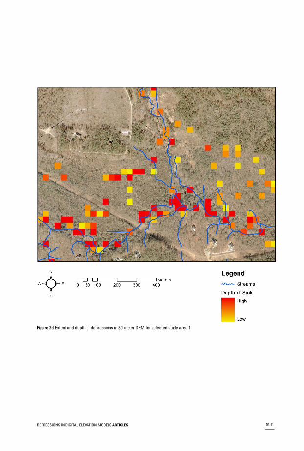
Figure 2d Extent and depth of depressions in 30-meter DEM for selected study area 1


Figure 2e Extent and depth of depressions in 61-meter DEM for selected study area 1

Figure 3a shows another type of study area, consisting of a more developed part of the wa-

tershed with low density residential development. Several man-made re/detention ponds are visiblewhich represent real depressions. [Note: this study area was chosen on purpose to show examplesof real depressions. Obviously, real depressions do not have to be ponds and can naturally occurin undeveloped areas, but these cannot always be identified easily on an orthophoto.] The slopegrid in Figure 3b confirms the presence of some well-defined banks around ponds, roads andbuildings, but otherwise the area is characterized by very smooth topography resulting from thegrading of the residential sub-division and the agricultural fields. Figures 3c, 3d, and 3e showthe extent and depth of the depressions based on DEMs of 6, 30 and 61 meters, respectively.The pattern in the depressions derived from the original 6-meter LIDAR DEM in Figure 3c reveals


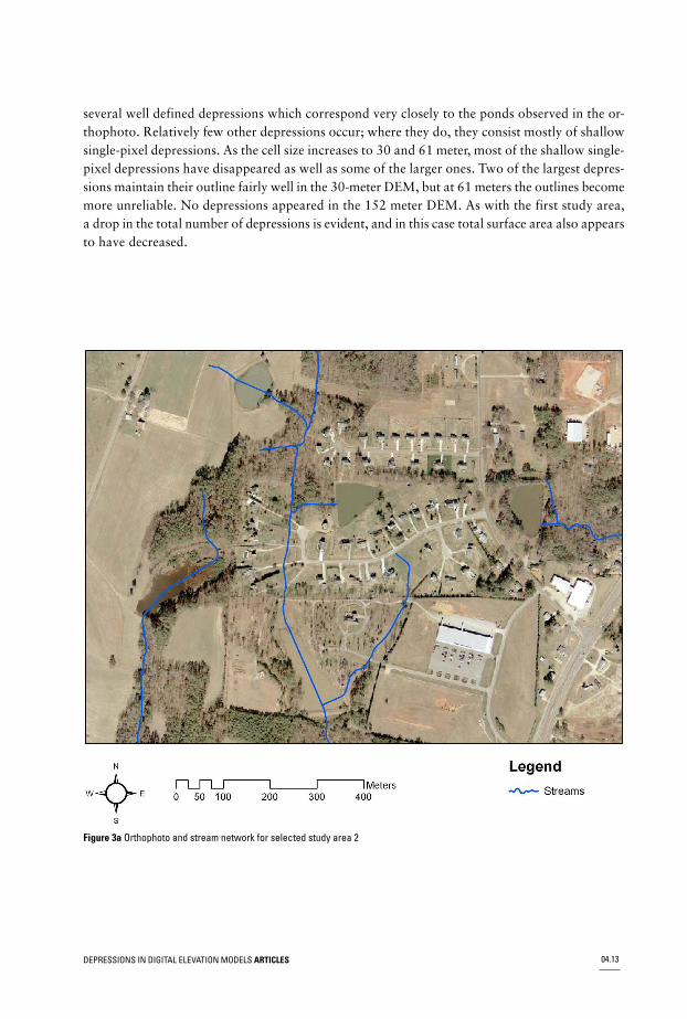
several well defined depressions which correspond very closely to the ponds observed in the or-thophoto. Relatively few other depressions occur; where they do, they consist mostly of shallowsingle-pixel depressions. As the cell size increases to 30 and 61 meter, most of the shallow single-pixel depressions have disappeared as well as some of the larger ones. Two of the largest depres-sions maintain their outline fairly well in the 30-meter DEM, but at 61 meters the outlines becomemore unreliable. No depressions appeared in the 152 meter DEM. As with the first study area,a drop in the total number of depressions is evident, and in this case total surface area also appearsto have decreased.

Figure 3a Orthophoto and stream network for selected study area 2


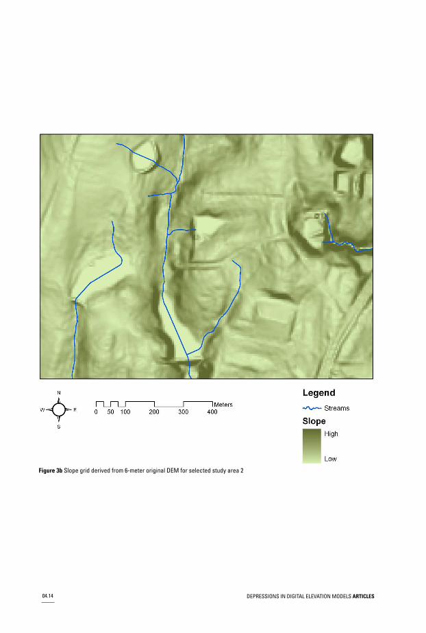
Figure 3b Slope grid derived from 6-meter original DEM for selected study area 2


Figure 3c Extent and depth of depressions in 6-meter original DEM for selected study area 2


Figure 3d Extent and depth of depressions in 30-meter DEM for selected study area 2


Figure 3e Extent and depth of depressions in 61-meter DEM for selected study area 2

The qualitative results so far provide a number of insights: 1) The number of depressionsappears to decrease with increasing cell size; 2) Many of the small and shallow depressions, whichare most likely artificial, disappear with increasing cell size, but a number of single-pixel depres-sions persist; 3) Trends in surface area and volume require more detailed quantification; and 4)Interpretation of results will require a consideration of artificial and real depressions.

Following this introductory visual characterization, a more rigorous quantitative descriptionis presented. First, Figure 4 shows the spatial extent of the depressions in the entire watershedfor selected resolutions. It confirms that the number of depressions decreases with increasing cellsize, but the changes in total surface area are less obvious. Statistical analyses presented in whatfollows all pertain to the entire watershed.


Figure 4 Extent of depressions in Middle Creek Watershed for selected DEM cell resolutions

Moving on to the more quantitative characterization of depressions, Figure 5 shows the rela-tionship between the number of depressions and cell resolution; a log scale is used for both axes.Table 1 reports the statistical summary for this data. Results reveal that the number of depressionsdecreases with cell resolution. Curve-fitting regression revealed an inverse power relationshipwith a very high degree of correlation. Table 2 reports the curve-fitting results – the results forsurface area and volume are included here and will be discussed in later sections.

The relationship between the number of depressions and cell resolution can be described as:number of depressions = 476,146* (cell size in meters) - 1.5098. The R-square for this regressionis 0.9988 and the relationship is significant with p < 0.0001. The power value for this relationshipis -1.5098.


Figure 5 Relationship between number of depressions and DEM cell resolution

Table 1 Descriptive statistics for depressions

Table 2 Non-linear regression results for depression characteristicsRegression model is based on an inverse power function: variable = A*(cell size)B

At first glance it may not seem very intuitive that the number of depressions for fine-scaleDEMs is much larger than for coarse-scale DEMs for the same area, since it is expected that fine-scale DEMs are more accurate in their representation of morphological features. However, itshould be recognized that the number of grid cells for a given area decreases by a power of 2


with increasing cell size. For example, a square parcel of land of 90,000 square meters would berepresented by 2500 cells in a 6-meter raster and by 25 cells in a 60-meter raster. For every 10-fold increase in cell size, the number of cells required to represent the exact same area is reduced100-fold, which is represented by a power factor of 2. The inverse power relationship betweenthe number of depressions and cell size, therefore, is not unexpected. What is somewhat surprising,however, is the fact that the power factor is much lower than 2. If the relation between thenumber of depressions and cell size were scale-independent, the power value would be exactly2, and it can therefore be inferred that the relationship is indeed scale-dependent. The fact thatthe power value is much less than two (i.e. 1.5098) is of significance, since this suggests that thenumber of depressions relative to the total number of cells in fact increases with large cell sizes.

The inverse power relationship between the number of depressions and cell size has implica-tions for how depressions are handled in terrain processing. As observed by Lindsay and Creed(2005b), the common practice of removing depressions prior to modeling flow networks usesalgorithms which rely on the identification of individual depressions prior to removal. These al-gorithms are currently at their limit in terms of DEM size, and despite increases in computingpower the depression removal techniques currently in use will not be able to process higher res-olution DEMs.

The number of depressions in the original 6-meter LIDAR DEM was 34,421 for the entirewatershed, or approximately 198 depressions per square kilometer. An even finer scale DEM offor example 3 meters would result in a depression density of approximately 500 depressions persquare kilometer. While 3 to 6 meters presents the current limit of most widely used LIDARDEMs, it does not seem impossible that with continued improvements in LIDAR collection andprocessing technology a cell resolution of 1 meter or even less might be used in the future. A 30cm DEM would have a depression density of approximately 16,500 depressions per squarekilometer, which presents serious challenges for current computing power.

While a number of depression filling algorithms exist, the one developed by Jenson andDomingue (1988) is by far the best known and has been implemented in nearly all GIS and hy-drologic software packages. Despite the widespread adoption of the Jenson and Domingue (1988)algorithm, the identification and filling of depressions remains the most time-consuming step inthe extracting stream networks and subwatersheds (Wang and Liu, 2006). Due to the relativelycomplex nature of the Jenson and Domingue (1988) algorithm and the large file size of theLIDAR DEM used in this study, none of the commercial GIS software with terrain analysisfunctions was able to process the LIDAR DEM for depression characterization within an accept-able time-frame. Processing of the LIDAR DEM for this study was therefore accomplished usingthe Planchon and Darboux (2001) algorithm, which is insensitive to data size and complexity.Both the Planchon and Darboux (2001) algorithm and the more recently developed Wang andLiu (2006) algorithm are expected to perform well with the large file sizes of LIDAR. These al-gorithms have not been implemented in commercial GIS and hydrologic software, but that canbe expected as processing of LIDAR data becomes more widespread. However, both these al-gorithms only address depression filling and do not consider alternative approaches to handledepressions such as breaching.

In addition to the number of depressions, the effect of cell size on the characteristics of de-pressions was determined by looking at the average area and the average volume of all depressions.Figure 6 shows the relationship between average depression area (in square meters) and cell size,


while Figure 7 shows the relationship between average depression volume (in cubic meters) andcell size.

Figure 6 Relationship between average area of depressions and DEM cell resolution

Figure 7 Relationship between average volume of depressions and DEM cell resolution

As could be expected based on the discussion of the number of depressions, both averagearea and average volume increase with larger cell sizes, revealing a power function. Curve-fittingregression results are reported in Table 2. Both relationships are very strong (R-square value of0.9907 and 0.9726, respectively) and highly significant (p < 0.0001 for both).


This general pattern was to be expected: as the DEM cell size increases, there are fewer de-pressions, but they are larger in size. The power relationships found reflects the same phenomenadescribed earlier: the number of grid cells for a given area decreases by a power of 2 with increas-ing cell size. Again, it is significant to note the power values: +1.7331 for average area and 2.3061for average volume. If the relationship was scale-independent these power values would be 2,and it can therefore be inferred that the relationships between cell resolution and average areaand volume are indeed scale-dependent.

In addition to exploring the effect of cell resolution on the average area of depressions interms of actual surface area, it is useful to explore the average size of depressions in terms of thenumber of cells. Figure 8 shows the relationship between the average size of depressions innumber of cells and cell resolution. Summary statistics are provided in Table 3.

Figure 8 Relationship between average size of depressions in number of cells and DEM cellresolution

Table 3 Summary statistics for the size distribution of depressions in number of cells


In general, many DEMs have a large number of very small depressions consisting of only oneor several cells, and a much smaller number of depressions consisting of a large number of cells.The DEMs used here are no exception to this, and the values for average size are fairly low.However, Figure 3 reveals a very surprising trend: the average number of cells per depressionfor the original 6-meter LIDAR DEM is 6.1 cells, but this drops off quickly to less than half thatwith increasing cell size, and levels out at around 1.6 cells at a cell size of around 61 meters. Thedescriptive statistics in Table 3 confirm that the maximum and standard deviation also decreasesubstantially with increasing cell size. These results suggest that the fine-scale DEMs are muchless dominated by single-cell depressions.

The pattern in Figure 3 requires some further consideration. The fact that for most of theDEM cell resolutions considered the value is between 1 and 2 is not surprising: the theoreticalminimum is one and single-pixel artificial depressions are often very dominant in DEMs. However,the much higher values for fine-scale DEMs suggest there is another phenomena at work. Thehypothesis presented here is that the original 6-meter LIDAR DEM contain a substantial numberof real depressions of relatively small size (i.e. several dozen to several hundred cells); some typ-ical examples are shown in Figure 3c, and may include man-made ponds as well as natural de-pressions. As the cell size increases, these real depressions are represented by a much lowernumber of cells or may disappear altogether, making them more difficult to distinguish fromartificial depressions. Therefore, the fine-scale DEMs are less dominated by single-cell depressionsand the average number of cells per depression is higher.

While this hypothesis explains the pattern observed in Figure 8 it should be pointed out thatproving this hypothesis requires that artificial and real depressions can be separated. At present,no such technique using only the DEM exists and intensive field verification would be requiredto accomplish this. At present, therefore, it remains a hypothesis for further research. It doeshowever, present some interesting new perspectives relevant for future research on depressions.For example, it suggests that many real depressions in landscapes might be relatively small,making them impossible to recognize in coarse-scale DEMs of 30 meters or larger. This emphasizesthe need to use high resolution DEMs to characterize depressional storage, particular in areasof moderate to low slopes. It also suggests that a technique to separate real from artificial depres-sions in a DEM should consider depression surface area as one of its criteria, but that the abilityto accomplish this is limited at coarse resolutions.

To further explore the size distribution of depressions, Figure 9 shows the cumulative distri-bution function of the number of depressions by depression size in cells. To maintain legibility,only the result for the original 6-meter LIDAR DEM and the 30-meter DEM are shown. Figure9 reveals that the coarser-scale DEM is indeed more dominated by smaller depressions. Thenumber of depressions of 1 cell as a percentage of the total number of depression is 56.6% forthe 6-meter DEM and 68.6% for the 30-meter DEM. Figure 9 reveals that this difference is fairlyconsistent across all depression sizes.


Figure 9 Cumulative distribution function of the number of depressions by depression size in cells for 6-meter and30-meter DEMs

Another meaningful and perhaps more insightful way to quantify the dominance of smalldepressions is to plot the cumulative distribution function of the depression area by depressionsize in cells. This is shown in figure 10, again only using the results for the original 6-meterLIDAR DEM and the 30-meter DEM. The area of depressions of 1 cell as a percentage of thetotal area of depressions is 9.2% for the 6-meter DEM and 30.4% for the 30-meter DEM. Figure10 reveals that this difference is fairly consistent across all depression sizes; however, at the upperend of the distribution the two curves approach each other as a result of the occurrence of onevery large depression. It should be noted that the curves in Figure 10 are not as smooth as inFigure 9; while in Figure 9 each depression is counted equally in determining the proportion, inFigure 10 each depression is weighted by its surface area, resulting in “jumps” in the distributionfor larger depressions.


Figure 10 Cumulative distribution function of the area of depressions by depression size in cells for 6-meter and30-meter DEMs

While the number of depressions and their size distribution provide a meaningful character-ization of the occurrence of depressions in DEMs of varying resolutions, ultimately of most interestare the total surface area and the total volume of depressions. These two parameters are mean-ingful in their own right for hydrological modeling since they provide information on the poten-tially available depressional storage in the landscape. They are also relevant for terrain processingsince they provide an indication of how much the original DEM needs to be modified in orderto become hydrologically correct. The scale-dependency of the relationship between cell size andthe number of depressions, as well as the scale-dependency of the size distribution of depressions,have already provided some indication that the total surface area and the total volume are notlikely to be scale-independent either. Figure 11 shows the relationship between the total surfacearea of depressions and cell size and Figure 12 shows the relationship between the total volumeof depressions and cell size.


Figure 11 Relationship between total surface area of depressions and DEM cell resolution

Figure 12 Relationship between total volume of depressions and DEM cell resolution

Both Figure 11 and 12 reveal scale-dependency of total surface area and total volume, respect-ively, but in somewhat surprising patterns. In Figure 11 the total surface area of depressions is7.8 square kilometers for the original 6-meter DEM, drops to 6.03 for 18 meters, appears toreach a minimum of 5.4 for 30 and 61 meters, and then gradually increases up to 20.1 square


kilometers for the 610-meter DEM. In Figure 12 the total volume of depressions is 2.6 millionm3 for the original 6-meter DEM, drops slightly to 2.1 and 2.0 million m3 for the 18 and 30-meter DEM, respectively, and then starts to gradually increase to 2.7 million m3 for the 61-meterDEM and ultimately to 76.7 million m3 for the 610-meter DEM. It should be recognized that ifthe surface area and volume were scale-independent, the curves in both Figures 11 and 12 wouldbe flat (i.e. straight lines with a slope of zero). The fact that they are not flat presents strongevidence of the scale-dependency of total depression area and volume.

In trying to find possible explanations for the scale-dependency of depression area and volume,it should be remembered that for many areas most depressions are expected to be artificial.Considering how artificial depressions are formed will provide some insights into the patternsfound in Figures 11 and 12.

The following explanation is presented for the observed scale-dependency of total area andtotal surface of depression. At the very highest resolution of 6 meters most of the small sinks (1to several cells) are likely artifacts – the DEM can be characterized by a very large number ofvery small and very shallow artificial depressions and a small number of larger and deeper truedepressions. As cell size increases to 30 or 61 meters, many of these small artificial depressionsdisappear since they are smaller than the new cell size; many (but fewer) small artificial depressionsremain (and some are newly created) as well as most of the larger and deeper real depressions.As a result, the total surface area of depressions drops. Since these small and artificial depressionsare very shallow, the effect on volume is much less strong; there is s small drop in depressionvolume going from 6 to 30 meters, but it is much less dramatic than for depression area.

As cell size increases from 61 to 152 meters and higher, small artificial depressions and somelarger real depressions disappear, but new large artificial depressions are created. In many areasthe cell resolution becomes insufficient to properly represent the variability in the terrain withinthe river channels. Minor channels which were well defined at the 30 or 61 meters resolutionbecome much less well defined, and many artificial depressions are created in and around thestream channel. As cell size increases to 305 meters and higher, even larger channels loose theirdefinition and very large artificial depressions are created.

This explanation suggests that there are two effects at work, both related to how artificialdepressions are formed: 1) For a very small cell size of 6 meters, the elevation difference betweenadjacent cells becomes very small and in many areas starts to approximate the vertical error ofthe elevation values. For this DEM the estimated vertical error is around 15 centimeters, whichcan be considered quite small for elevation data. Nevertheless, this small vertical error appearsto result in a large number of small and shallow artificial depressions at the original resolution.As the DEM gets coarser, this effect becomes less and artificial depressions start to disappear.2) For larger cell sizes (100 meters and higher) much of the spatial variability in elevation is lostand major channels loose their definition. This results in some very large and deep artificial de-pressions which because of their size have a strong influence on the total surface area and totalvolume of all depressions combined.

The first effect has been illustrated already in Figures 2c, 2d and 2e. The second effect is illus-trated in Figure 13a, 13b and 13c, which show the extent and depth of depressions as well asthe slope derived from DEMs of 6, 30 and 152 meters, respectively. The purple line representsthe cross section used later in Figure 14.


Figure 13a Depressions and slope derived from 6-meter original LIDAR DEM


Figure 13b Depressions and slope derived from 30-meter DEM


Figure 13c Depressions and slope derived from 152-meter DEM

Figure 13a shows the somewhat typical pattern for the depressions in the original 6-meterLIDAR DEM: a large number of small and relatively shallow depressions, as well as some largerand deeper ones close to the stream. The results in Figure 13b for 30 meters represent the firsteffect mentioned above: fewer depressions but covering a similar total area. As can be seen in


the results for the slope grid, at the highlighted cross section the stream channel is very narrow(1 or 2 cells) but still clearly defined. The slope grid for 152 meters in Figure 13c shows that thestream channel definition has been lost – it appears as if the channel has “collapsed”. As a result,a very large and deep artificial depression is created.

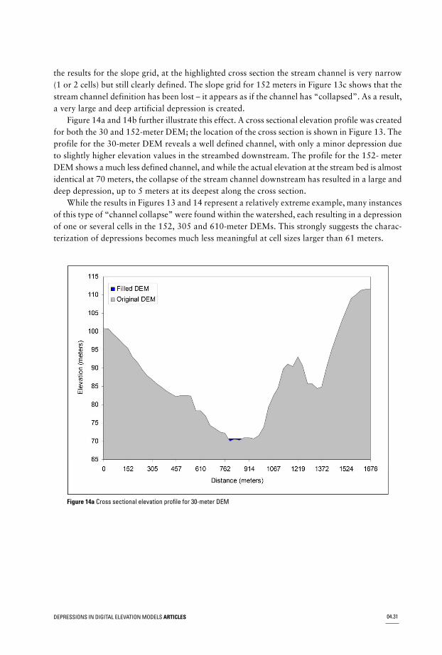
Figure 14a and 14b further illustrate this effect. A cross sectional elevation profile was createdfor both the 30 and 152-meter DEM; the location of the cross section is shown in Figure 13. Theprofile for the 30-meter DEM reveals a well defined channel, with only a minor depression dueto slightly higher elevation values in the streambed downstream. The profile for the 152- meterDEM shows a much less defined channel, and while the actual elevation at the stream bed is almostidentical at 70 meters, the collapse of the stream channel downstream has resulted in a large anddeep depression, up to 5 meters at its deepest along the cross section.

While the results in Figures 13 and 14 represent a relatively extreme example, many instancesof this type of “channel collapse” were found within the watershed, each resulting in a depressionof one or several cells in the 152, 305 and 610-meter DEMs. This strongly suggests the charac-terization of depressions becomes much less meaningful at cell sizes larger than 61 meters.

Figure 14a Cross sectional elevation profile for 30-meter DEM


Figure 14b Cross sectional elevation profile for 152-meter DEM

CONCLUSIONSResults of this study indicate that DEM cell resolution has a very strong effect on the occurrenceof depressions. The number of depressions was found to increase with smaller cell size followingan inverse power relationship. The power factor of 1.51 strongly suggest that the relationship isscale-dependent and not simply determined by the increased number of cells in the DEM for thesame study area. The inverse power relationship between the number of depressions and cell sizehas implications for how depressions are handled in terrain processing, and it is expected thatmost GIS software being used for terrain analysis will need to adopt revised algorithms for de-pression removal in order to process high resolution LIDAR DEMs.

Both average area and average volume of depressions were found to increase with larger cellsize, revealing a power function. This supports the general expectation that coarse scale DEMsare dominated by fewer but larger depressions. The power factors of 1.73 and 2.31 for averagearea and average volume, respectively, again indicate strong scale-dependency.

Scale-dependency was also found for the total area and total volume of depressions, but thepatterns are more complicated. Both decreased from the original 6-meter LIDAR DEM to 30and 61 meters, and increased for coarser-scale DEMs. An explanation based on the formationof artificial depressions has been presented.

Based on the results for this study area, there appears to be “sweet spot” around 30 to 61meters where the amount of depressions in terms of surface area and volume is at a minimum.In this resolution range there will still be many artificial depressions, but their presence is lessthan at finer or coarser scales. At finer scales, the (small) vertical error of the DEM needs to be


considered and introduces a large number of very small and very shallow artificial depressions.At coarser scales, the terrain structure is no longer reliably represented and a substantial numberof large and sometimes deep artificial depressions is created.

The results presented here support the conclusion that the use of the highest resolution andmost accurate data, such as LIDAR DEMs, may not result in the most reliable estimates of terrainderrivatives unless proper consideration is given to the scale-dependency of the parameters beingstudied. The results also suggest that further research into depression removal techniques forhigh resolution DEMs is needed, as well as a characterization of the scale-dependency of artificialand real depressions for different landscape types.

REFERENCESBarber, C; Shortridge, A. 2005. ‘LIDAR elevation data for surface hydrologic modeling: Resolution and

representation issues’. Cartography and Geographic Information Science 32 (4): 401–410.Brasington, J; Richards, K. 1998. ‘Interactions between model predictions , parameters and DTM scales for

TOPMODEL’. Computers and Geosciences 24 (4): 299–314.Claessens, L; Heuvelink, G; Schoor, J; Veldkmap, A. 2005. ‘DEM resolution effects on shallow landslide

hazard and soil redistribution modeling’. Earth Surface Processes and Landforms 30: 461–477.Clarke, S; Burnett, K. 2003. ‘Comparison of digital elevation models for aquatic data development’.

Photogrammetric Engineering and Remote Sensing 69 (12): 1367–1375.Fairfield, J; Leymarie, P. 1991. ‘Drainage networks from grid digital elevation models’. Water Resources

Research 27 (5), 709–717.Florinsky, I.V.2002. ‘Errors of signal processing in digital terrain modeling’. International Journal of

Geographical Information Science 15 (5): 475–501.Garbrecht J.; Martz, L. 2000. ‘Digital elevation model issues in water resources modeling’. In: Hydrologic

and hydraulic modeling support with Geographic Information Systems, D. Maidment and D. Djokic(eds.), pp. 1–27. ESRI Press, Redlands, CA.

Goodchild, M; Mark, D.M. 1987. ‘The fractal nature of geographic phenomena’. Annals of the Associationof American Geographers 77 (2): 265–278.

Hancock, G.R. 2005. ‘The use of DEMs in the identification and characterization of catchment over differentgrid scales’. Hydrological Processes 19: 1727–1749.

Hayashi, M; van der Kamp, G. 2000. ‘Simple equations to represent the volume-area-depth relationships ofshallow wetlands in small topographic depressions’. Journal of Hydrology 237: 74–85.

Horne B.K.P. 1981. ‘Hill shading and the reflectance map’. Proceedings of the IEEE 69 (1): 14–47.Hutchinson, M.F. 1989. ‘A new procedure for gridding elevation and stream line data with automatic removal

of spurious pits’. Journal of Hydrology 106: 211–232.Jenson, S; Domingue, J.O. 1988. ‘Extracting topographic structure from digital elevation data for geographic

information system analysis’. Photogrammetric Engineering and Remote Sensing 54 (11): 1593–1600.Kenward, T; Lettenmaier, D; Wood, E; Fielding, E. 2000. ‘Effects of digital elevation model accuracy on

hydrologic predictions’. Remote Sensing of the Environment 74: 432–444.Kienzle, S. 2004. ‘The effect of DEM raster resolution on first order, second order and compound terrain

derivatives’. Transaction in GIS 8 (1): 83–111.Liang, C; Mackay, D.S. 2000. ‘A general model of watershed extraction and representation using globally

optimal flow paths and up-slope contribution areas’. International Journal of GeographicalInformation Science 14 (4): 337–358.

Lindsay, J; Creed, I.F. 2005. ‘Removal of artifact depressions from digital elevation models: Towards aminim impact approach’. Hydrological Processes 19: 3113–3126.


Lindsay, J; Creed, I.F. 2005. ‘Sensitivity of digital landscapes to artifact depressions in remotely-sensedDEMs’. Photogrammetric Engineering and Remote Sensing 71 (9): 1029–1036.

Lindsay, J; Creed, I. 2006. ‘Distinguishing actual and artifact depressions in digital elevation data’. Computersand Geosciences (in press).

MacMillan, R; Marti, T; Earle, T; McNabb, D.H. 2003. ‘Automated analysis and classification of landformsusing high resolution digital elevation data: Applications and issues’. Canadian Journal of RemoteSensing 29 (5): 592–606.

Mark, D.M. 1984. ‘Automatic detection of drainage networks from digital elevation models’. Cartographica21: 168–178.

Marks, D; Dozier, J; Frew, J. 1984. ‘Automated basin delineation from digital elevation data’. Geo-Processing2: 299–311.

Martz, L; Garbrecht, J. 1998. ‘The treatment of flat areas and depressions in automated drainage analysisof raster digital elevation models’. Hydrological Processes 12: 843–855.

Martz, L; Garbrecht, J. 1999. ‘An outlet breaching algorithm for the treatment of closed depressions in araster DEM’. Computer and Geosciences 25: 835–844.

Martz, L; Jong, E.D. 1988. ‘CATCH: A Fortran program for measuring catchment area from digital elevationmodels’. Computers and Geosciences, 14: 627–640.

McCormack, J; Gahegan, M; Roberts, S; Hogg, J; Hoyle, B.S. 1993. ‘Feature-based derivation of drainagenetworks’. International Journal of Geographical Information Systems 7 (3): 263–279.

McMaster, K.J. 2002. ‘Effects of digital elevation model resolution on derive strem network positions’. WaterResources Research 38 (4): 13-1–13-8. DOI: 10.1029/2000WR000150

North Carolina Flood Mapping Program. 2006. Issues Papers of the North Carolina Cooperating TechnicalState Flood Mapping Program. Accessed online on April 6, 2006 athttp://www.ncgs.state.nc.us/floodmap.html.

North Carolina Flood Mapping Program. 2002. LIDAR Accuracy Assessment Report – Wake County.Accessed online on April 6, 2006 at http://www.ncgs.state.nc.us/floodmap.html.

North Carolina Flood Mapping Program. 2001. Issues 7: LIDAR Specifications. Accessed online on April6, 2006 at http://www.ncgs.state.nc.us/floodmap.html.

O’Callaghan, J; Mark, D.M. 1984. ‘The extraction of overland flow networks from digital elevation data’.Computer Vision, Graphics and Image Processing 28: 323–344.

Oksanen, J; Sarjakoski, T. 2005. ‘Error propogation analysis of DEM-based drainage basin delineation’.International Journal of Remote Sensing 26 (14): 3085–3102.

Planchon, O; Darboux, F. 2001. ‘A fast, simple algorithm to fill the depressions of digital elevation models’.Catena 46: 159–176.

Rosenberry, D; Winter, T.C. 1997. ‘Dynamics of water-table fluctuations in an upland between twoprairie-pothole wetlands in North Dakota’. Journal of Hydrology 191: 266–289.

Schoorl, J; Sonneveld, M; Veldkamp, A. 2000. ‘Three-dimensional landscape process modellilng: The effectof DEM resolution’. Earth Surface Processes and Landforms 25: 1025–1034.

Thompson, J; Bell, J; Buttlet, C.A. 2001. ‘Digital elevation model resolution: effects on terrain attributecalculation and quantitative soil-landscape modeling’. Geoderma 100: 67–89.

Thieken, A; Lucke, A; Diekkruger, B; Richter, O. 1999. ‘Scaling input data by GIS for hydrological modelling’.Hydrological Processes 13: 611–630.

Tribe, A. 1991. ‘Automated recognition of valleylines and drainage networks from grid digital elevationmodels: a review and a new method’. Journal of Hydrology 139: 263–293.

Usery, E; Finn, M; Scheidt, D; Ruhl, S; Beard, T; Bearden, M. 2004. ‘Geospatial data resampling and resolutioneffects on watershed modeling: A case study using the agricultural non-point source pollution model’.Journal of Geographical Systems 6: 289–306.

Walker, J; Willgoose, G.R. 1999. ‘On the effect of digital elevation model accuracy on hydrology andgeomorphology’. Water Resources Research 35 (7): 2259–2268.


http://www.ncgs.state.nc.us/floodmap.html



Wang, L; Liu, H. 2006. ‘An efficient method for identifying and filling surface depressions in digital elevationmodels for hydrologic analysis and modeling’. International Journal of Geographical InformationScience 20 (2): 193–213.

Wang, X; Yin, Z. 1998. ‘A comparison of drainage networks derived from digital elevation models at twoscales’. Journal of Hydrology 210: 221–241.

Wolock, D; McCabe, G.J. 2000. ‘Differences in topographic characteristics computed from 100 and 1000meter resolution DEM data’. Hydrological Processes 14: 987–1002.

Zhan, X; Drake, N; Wainwright, J; Mulligan, M. 1999. ‘Comparison of slope estimates from low resolutionDEMs: Scaling issues and a fractal method for their solution’. Earth Surface Processes and Landforms24: 763–779.

Zhang, W; Montgomery, D.R. 1994. ‘Digital elevation model grid size, landscape representation andhydrologic simulations’. Water Resources Research 30 (4): 1019–1028.

Cite this article as: Zandbergen, Paul. ‘The effect of cell resolution on depressions in Digital ElevationModels’. Applied GIS 2 (1). pp. 4.1–4.35. DOI: 10.2104/ag060004.


Documents

The effect of cell resolution on depressions in Digital ... · PDF file2002). The occurrence of ... (Wang and Liu, 2006). However, depression filing can sometimes result in substantial