The Effect of Bank Credit on Asset Prices: Evidence from the Japanese Real Estate Boom during the 1980s

NADA MORA

The Effect of Bank Credit on Asset Prices:

Evidence from the Japanese Real Estate

Boom during the 1980s

This paper studies whether bank credit fuels asset prices. Financial dereg-ulation during the 1980s allowed keiretsus to obtain finance publicly andreduce their dependence on banks. Banks that lost these blue-chip customersincreased their property lending, and serve as an instrument for the supplyof real estate loans. Using this instrument, I find that a 0.01 increase in aprefecture’s real estate loans as a share of total loans causes 14–20% higherland inflation compared with other prefectures over the 1981–91 period. Thetiming of losses of keiretsu customers also coincides with subsequent landinflation in a prefecture.

JEL codes: E44, G21, G28Keywords: bank credit, asset prices, financial regulation.

THE PURPOSE OF THIS paper is to determine whether bank creditaffects asset prices. The Japanese real estate boom during the 1980s provides a uniqueepisode to help answer this question. In particular, this paper studies the extent towhich an exogenous shock to the supply of bank credit fuels land prices. I showthat I have an instrument for the supply of real estate loans, which is the decreasein banks’ loans to keiretsu firms beginning in the early 1980s. I then take advantageof the cross-sectional and time-series variation in Japan’s 47 prefectures. Using this

I am indebted to David Weinstein and Hugh Patrick for giving me the opportunity to be a visitingscholar at the Center on Japanese Economy and Business (CJEB) at Columbia Business School duringthe summer of 2004 and for many helpful conversations. I would like to acknowledge David Weinsteinfor providing me with access to the Development Bank of Japan Corporate Finance Data Set and theCJEB for providing me with access to the Nikkei NEEDS database. I thank Takeo Hoshi for sharing hisdata and for his initial encouragement to pursue this topic. I also benefited from comments from RicardoCaballero, Roberto Rigobon, James Vickery, Sujit Kapadia, Deborah Lucas (the Editor), an anonymousreferee, participants at the MIT International Workshop, the 22nd Symposium on Banking and MonetaryEconomics in Strasbourg, and the 18th Australasian Finance and Banking Conference in Sydney.

NADA MORA is an Assistant Professor in Economics Department, The American Universityof Beirut (E-mail: [email protected]).

Received August 8, 2005; and accepted in revised form February 22, 2007.

Journal of Money, Credit and Banking, Vol. 40, No. 1 (February 2008)C© 2008 The Ohio State University

58 : MONEY, CREDIT AND BANKING

instrument, I find that a 0.01 increase in a prefecture’s real estate loans as a share oftotal loans causes 14–20% higher land inflation over the 1981–91 period. The timingof losses of keiretsu customers also coincides with subsequent land inflation in aprefecture.

There is consensus in the literature on Japan that a shock in the 1980s led banksto increase lending in the real estate sector. The regulatory change that decreasedthe demand for loans by keiretsus is a candidate for that shock. The first part of thispaper shows that lending to keiretsus declined as a result of the financial deregulation,which enabled keiretsu firms to obtain financing from the public market. This supportsthe Hoshi and Kashyap (2000, 2001) (hereafter HK) hypothesis, which is that largeand well-known firms (mostly keiretsus) substantially reduced their dependence onbank financing by issuing bonds during the 1980s. Therefore it was a choice by firmsto move away from banks. In contrast, the “good opportunities” hypothesis wouldimply that banks chose to move away from keiretsu firms. Real estate may have beenperceived to have good opportunities, rationalizing a shift of bank lending to the realestate sector during the 1980s.1 The results of extensive tests do not suggest that thiswas the case in Japan.

The regulatory change during the 1980s was not the first to change the financiallandscape in Japan. The history of the Japanese financial system runs contrary to thepopular opinion that it is unique in its emphasis on banks. This has been a relativelyrecent phenomenon. The history of the system evolved as an outcome of regulatorychanges, which in turn were endogenous to macroeconomic shocks. Among the moreimportant shocks to the Japanese economy were World War II and the oil shocksin the 1970s (see Hoshi and Kashyap 2001). It is interesting that firms (includingsmall and medium size enterprises) funded themselves mostly through the capitalmarket from the Meiji restoration until the 1930s. For example, the share of bondand equity finance in the external sources of funds for non-financial firms reached0.7 in 1935 (Ueda 1994). The government’s motivation to restrict competition wasa result of the 1930s and war. It was at this time that the government took controlof the allocation of credit and used banks to implement its preference toward fundingthe military. During the Japanese miracle period from the 1950s to the early 1970s,the government’s priority shifted from the military to industry. As a result, the systemdid not revert to the pre-war emphasis on capital markets. The savings restrictions onhouseholds guaranteed the flow of funds to the banks, which in turn channeled themto keiretsus.

It was only with the development of the Japanese corporate bond market thatkeiretsus decreased their demand for bank loans. I establish that this shock can beused to assess whether bank credit affects asset prices. The main part of the paperthen explains the Japanese bubble in land prices and its differential impact acrossJapan’s prefectures using the keiretsu loan shock as an instrument. When banks lost

1. A third view emphasizes monetary factors which can be related to the “good opportunities” view.For example, Ueda (2000) argues that monetary policy was responsible for the wide swings in asset pricesthat caused increased bank lending toward real estate.

NADA MORA : 59

their keiretsu customers, they increased their lending to the real estate sector and thatin turn fueled land prices.

Previous papers assessing why banks in Japan increased their real estate lendingduring the 1980s take land prices as given, overlooking the idea that the increase ofbank credit in real estate may itself have contributed to aggregate land price inflation.In standard asset pricing models with no credit market imperfections, the willingnessof banks to offer loans would have no impact on asset prices. Therefore, the presenceof credit constraints is fundamental to the empirical analysis in this paper. Kiyotakiand Moore (1997) provide a useful frame of reference. They assign a dual role toassets: they are not just factors of production, but also serve as collateral for loans.As a result, credit limits are affected by asset prices. Therefore, a firm’s borrowingcapacity and its demand for credit will be affected by changes in asset prices. Apositive productivity shock causes land prices to increase and raises the net worth offirms. This allows firms to borrow more, leading to a demand for land that increaseswith its price.2

However, this paper is concerned with the effects of allowing for shocks to thesupply of loans. In a separate note which extends the analysis in Kiyotaki and Moore(1997),3 I show that asset prices (and asset holdings) can also be affected by shocksto credit limits. A similar credit cycle is created when banks ease binding credit limitsindependently of firms’ net worth, allowing them to borrow more, invest more in theasset, and hence drive up the price of the asset.

Gerlach and Peng (2005) note that there can be a role for credit in asset valuations,an idea which goes back to Kindleberger (1978). This is also in the spirit of Ito andIwaisako (1996). In a setup with asymmetric information, they show that the extent towhich banks are willing to extend credit matters for projects that require acquisitionof land or stocks. Using a VAR, they find that total bank loans to real estate leadthe aggregate real land price in Japan, while only current land price inflation helpsexplain the growth of bank loans. Gerlach and Peng find instead that the directionof influence goes from demand and property prices to bank credit when looking ataggregate data from Hong Kong.

The main contribution of this paper is in isolating the effect of bank credit onreal estate prices using an instrument for the supply of real estate loans. A secondcontribution is in applying the analysis to dis-aggregated data. The results are relevantto the current policy debate on land price inflation, and the role of banks in fuelingreal estate lending. The closest paper to this one is Peek and Rosengren (2000), whichstudies the effect of an exogenous negative loan supply shock (originating in Japan)on the United States. They find that the decline in Japanese bank lending contributedto a substantial decline in new construction projects in the US.

The rest of this paper is organized as follows: Section 1 tests whether the fallin keiretsu loans was driven by firms or banks; having determined that the evidence

2. It is for this reason that a positive productivity shock causes the constrained borrowers to demandmore credit and invest more. In contrast, the first-best allocation is not affected and the only outcome isthat agents increase their consumption.

3. Available on author’s website, http://alum.mit.edu/www/namora.


supports the former, Section 2 assesses whether, and to what extent, bank credit affectsland prices; Section 3 concludes.

1. THE FALL IN LENDING TO KEIRETSUS: FIRM OR BANK CHOICE?

Japan liberalized its financial system in the 1980s. As part of this deregulation,firms reduced their borrowing from banks. The HK hypothesis is that large and well-known firms substantially reduced their dependence on bank financing by issuingbonds during the 1980s (with the market substituting reputation for monitoring). Incontrast, the “good opportunities” hypothesis implies that banks chose to move awayfrom keiretsus to the more promising real estate sector.

In this section, I briefly summarize existing evidence for the HK hypothesis, i.e., theidea that the development of the Japanese corporate bond market caused an exogenousfall in demand for bank loans, which then fueled an increase in bank real estate lending(as shown in Figure 1). I then present new evidence consistent with the HK hypothesisusing both bank-level and firm-level data.

1.1 Previous Literature

Hoshi and Kashyap articulate their view in several papers, drawing several stylizedfacts from data on publicly traded Japanese firms (Hoshi and Kashyap 2000, 2001).First, there was a substantial decrease in bank borrowing among large firms, andparticularly manufacturing firms. The ratio of bank debt to total assets for large

FIG. 1. Keiretsu Loans, Loans to Listed Firms, and Loans to Real Estate Sector (as a Share of Total Loans, All Banks,Average).

NOTES: Source: The keiretsu loans and loans to listed firms were provided by Takeo Hoshi, who compiled them fromKeizai Chosakai, Kin’yu Kikan no Toyushi (Investment and Loans by Financial Institutions), various issues. The real estateloans and the total loans come from the Nikkei NEEDS database.

NADA MORA : 61

manufacturing firms fell from 0.35 in the 1970s to below 0.15 by 1990. Second, firmsreplaced bank loans with bond financing. Third, the shift appears to have occurredrelatively soon after they became eligible to do so. There was rationing in the corporatebond market prior to 1976. Beginning that year, a firm could issue as many bondsas it chose provided that it met specific accounting criteria (see the Appendix andTable A3 for details). Hoshi and Kashyap also find that banks which relied moreheavily on customers with access to capital markets subsequently under-performedcompared with other banks.

Hoshi (2001) tests the hypothesis in two steps using individual bank data. He findsthat banks that increased the proportion of loans to the real estate sector during the1980s ended up with a higher non-performing loan ratio in 1998. He then uses apanel of 150 banks to regress the change in a bank’s real estate loan ratio on laggedchanges in keiretsu loan ratios, controlling for land prices and year effects. Banksexperiencing a greater decline in their keiretsu loan share subsequently increasedtheir real estate loans during the 1980s. Although this offers support for the HKview, it does not rule out the “good opportunities” view. It is better to distinguishbetween the two hypotheses using firm data, and I will take this up in Section 1.2below.

Hoshi, Kashyap, and Scharfstein (1993) document that the share of bank debt forthe 112 firms that were permitted to continuously issue convertible bonds from 1982to 1989 was lower and increasingly so as compared with the remaining 424 firmsin their sample. Weinstein and Yafeh (1998) emphasize the holdup problem of firmsby banks prior to liberalization. They find that although close bank-firm ties increasethe availability of capital to manufacturing firms, the associated cost of capital ishigher. Much of the difference in capital use between affiliated and unaffiliated firmsdisappeared by 1981. They interpret this as evidence supporting the importance ofthe liberalization of the foreign exchange law in 1980.

Even if firms reduced their borrowing from banks in favor of bond markets, it doesnot fully explain the shift of banks to real estate. Faced with a decrease in demand forbank loans from keiretsus, other alternatives include looking for other loans, investingin government bonds, seeking foreign opportunities, or choosing to reduce depositrates and shrink in size. These possibilities are considered in Section 1.2, but first Isummarize the existing literature.

Hoshi and Kashyap argue that gradual deregulation, combined with the policy oflimited liability, can explain why banks did not shrink as they lost their keiretsucustomers. One implication of the gradual deregulation was that households hadlimited savings options and continued to channel their funds to banks. When combinedwith interest rate controls to ensure positive profit margins and a policy of governmentdeposit guarantees, banks attempted to make up through volume the decrease inmargins during this period. The “convoy” system in Japan ensured that no bank wasallowed to go bankrupt. Therefore the government assumed banks’ credit risk. As themain bank system receded in importance, it was not effectively replaced with a properregulatory system to evaluate and monitor risk-taking by banks. Further implicationsof deregulation are highlighted in the Appendix. Variations of these arguments are


also raised by Kitigawa and Kurosawa (1994) and Cargill, Hutchison, and Ito (1997),among others.

To explain why banks predominantly moved to real estate and not to other typesof loans, government bonds or foreign opportunities, Hoshi (2001) argues that banksrelied on collateralized loans because they lacked close knowledge of new customers.Land was considered the most secure collateral because its value had not fallen inthe post-war period. Therefore a plausible explanation is that banks may (on average)have wrongly perceived low volatility in real estate. This view is echoed by Ueda(1994), who contends that banks actively competed for loans related to real estatebecause credit analysis was considered relatively easy as it consisted of forecastingfuture land prices, and these prices were expected to increase.

The actions of the Bank of Japan and the Ministry of Finance during the real estateboom are also interesting. Ueda (1994) argues that although the Bank of Japan andthe Ministry of Finance were concerned about the increase in land prices, they didnot try to stop it because the general price level was stable and they were unableto foresee the collapse. Only in April 1990 did they introduce quantitative controlslimiting bank lending in real estate. Ito (2004) suggests that this action contributedto the end of the land bubble. This supports the contention that it was a bank-led realestate boom as opposed to one driven by real estate demand.

1.2 New Empirical Tests on Firm or Bank Choice

Stylized evidence. I now present new evidence consistent with the HK hypothesis.Firm survey data provide insight into whether keiretsus chose to reduce bank loans orvice versa. The Bank of Japan conducts a quarterly survey of enterprises with ques-tions on short-term economic conditions, known as the Tankan survey. One of thequestions asks firms to assess the lending attitudes of financial institutions. Figure 2shows the “diffusion” index for manufacturing and real estate & construction enter-prises, respectively. Large manufacturing enterprises serve as a proxy for keiretsus. Ahigher value of the index indicates that more firms perceived accommodative lendingconditions. If the “good opportunities” hypothesis were correct, it would be expectedthat the index (or its difference) for real estate and construction firms would be higherthan that for large manufacturing firms during the 1980s. This is not the case. In fact,during the first part of the 1980s when the share of bank loans to keiretsus declinedfrom around 0.15 to 0.05 (Figure 1), large manufacturing enterprises reported in-creasingly accommodative lending attitudes in contrast to the stable lending attitudesperceived by construction and real estate firms.

Table 1 presents evidence on the source of flow of funds to the real estate marketbased on data reported in Cargill, Hutchison, and Ito (1997). If large real estatecompanies with the ability to borrow in the bond market were fueling the boom, banklending would not be expected to be the dominant means of financing real estateinvestment. It turns out that banks accounted for the principal source of funds (59 outof 120 trillion yen total at the peak of the boom in June 1991). Non-bank financialinstitutions accounted for another 50–55 trillion yen; insurance companies, creditunions, and foreign banks accounted for 9.1; and only a residual of 2 came from

NADA MORA : 63

FIG. 2. Tankan Survey: Perception by Enterprises of Financial Institutions’ Lending Attitudes (A Higher NumberIndicates Perception of More Relaxed Conditions).

NOTES: Source: Bank of Japan, Research and Statistics Department, http://www.boj.or.jp/en. For judgement questions, thepercentage share of the raw number of responding enterprises for each of the three choices is calculated. The diffusionindex (DI) is calculated as following: DI = percentage share of enterprises responding for choice 1 minus percentageshare of enterprises responding for choice 3. The choices for lending attitude were (i) accommodative choice (ii) not sosevere, and (iii) severe. Therefore if all the surveyed enterprises perceived the lending attitude to be accomodative, theindex would be equal to 100 and vice versa.

TABLE 1

FLOW OF FUNDS TO THE REAL ESTATE MARKET (TRILLIONS OF YEN) JUNE 1991

Credit TotalDomestic Insurance unions & Foreign Non- Capital to real

banks companies depository banks banks market estate

Direct financing 59 3 5.5 0.6 50–55 Residual 120(maximum 2)

Indirect lending activities throughnon-bank financial institutions

72 15 0.6 6.3

NOTE: Taken from Figure 5.6 in Cargill, Hutchison, and Ito (1997), who obtained the data from the Ministry of Finance.

the capital markets. It is important to note that a major share of non-bank financialinstitutions were specialized housing loan companies created as subsidiaries of banksin the 1970s (known as “jusen”). Therefore if we account for the indirect flow of fundsfrom banks to real estate via non-banks, banks would account for the vast majorityof the flow of funds to real estate (since 72 trillion yen is reported to be the flow offunds from banks to non-banks).


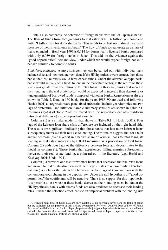
Table 1 also compares the behavior of foreign banks with that of Japanese banks.The flow of funds from foreign banks to real estate was 0.6 trillion yen comparedwith 59 trillion yen for domestic banks. This needs to be first normalized by a validmeasure of their investments in Japan.4 The flow of funds to real estate as a share ofloans extended in fiscal year 1991 is 0.114 for domestically licensed banks comparedwith only 0.039 for foreign banks in Japan. This adds to the evidence against the“good opportunities” demand view, under which we would expect foreign banks tobehave similarly to domestic banks.

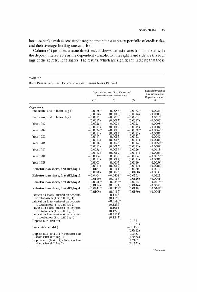
Bank-level evidence. A more stringent test can be carried out with individual bankbalance sheet and income statement data. If the HK hypothesis were correct, then thosebanks that lost keiretsus would have excess funds. Under the alternative hypothesis,banks would actively seek funds to lend in the real estate sector, as the return on theseloans was greater than the return on keiretsu loans. In this case, banks that increasetheir lending to the real estate sector would be expected to increase their deposit rates(and quantities of borrowed funds) compared with other banks. Regression results areshown in Table 2. Data on 150 banks for the years 1983–90 are used and followingHoshi (2001) all regressions are panel fixed effects that include year dummies and twolags of prefectural land inflation. Sample summary statistics are shown in Table A1.Columns (1)–(3) of Table 2 are estimated with the real-estate-loans-to-total-loansratio (first difference) as the dependent variable.

Column (1) is a similar model to that shown in Table 9.1 in Hoshi (2001). Fourlags of the keiretsu loan share (first difference) are included on the right-hand side.The results are significant, indicating that those banks that lost more keiretsu loanssubsequently increased their real estate lending. The estimates suggest that for a 0.01annual decrease (over 4 years) in a bank’s share of keiretsu loans to total loans, itslending in real estate increases by 0.0013 measured as a proportion of total loans.Column (2) adds four lags of the difference between loan and deposit rates to themodel in column (1). Those banks that experienced falling margins subsequentlyincreased their real estate lending, a point raised in the literature (e.g., Hoshi andKashyap 2001; Ueda 1994).

Column (3) provides one test for whether banks that decreased their keiretsu loansand moved to real estate also increased their deposit rates to obtain funds. Therefore,column (3) includes the interaction between the four lags of keiretsu loans with thecontemporaneous change in the deposit rate. Under the null hypothesis of “good op-portunities,” the coefficients will be negative. There is no support for this hypothesis.It is possible to test whether these banks decreased their lending rates, but under theHK hypothesis, banks with excess funds are also predicted to decrease their lendingrates. Further, the selection effect leads to an empirical problem with the lending side

4. Foreign bank flow of funds data are only available at an aggregate level from the Bank of Japanbut are sufficient for the purpose of this stylized comparison. Refer to “Detailed Data of Flow of FundsAccounts” available from the Bank of Japan, http://www.boj.or.jp/en. It provides information on total loansextended by domestically licensed banks and foreign-owned banks in Japan, respectively, in the section“Loans by Private Financial Institutions (Book Value)”.

NADA MORA : 65

because banks with excess funds may not maintain a constant portfolio of credit risks,and their average lending rate can rise.

Column (4) provides a more direct test. It shows the estimates from a model withthe deposit interest rate as the dependent variable. On the right-hand side are the fourlags of the keiretsu loan shares. The results, which are significant, indicate that those

TABLE 2

BANK REGRESSIONS: REAL ESTATE LOANS AND DEPOSIT RATES 1983–90

Dependent variable: First difference of:Dependent variable:

Real estate loans to total loansFirst difference of:

Deposit interest rate(1)a (2) (3) (4)

RegressorsPrefecture land inflation, lag 1b 0.0086∗∗ 0.0086∗∗ 0.0078∗∗ −0.0024∗∗

(0.0016) (0.0016) (0.0016) (0.0006)Prefecture land inflation, lag 2 −0.0013 −0.0008 −0.0005 0.0015∗

(0.0017) (0.0017) (0.0017) (0.0006)Year 1983 −0.0025∗ −0.0024 −0.0023 −0.0095∗∗

(0.0012) (0.0012) (0.0015) (0.0004)Year 1984 −0.0034∗∗ −0.0015 −0.0038∗∗ −0.0062∗∗

(0.0011) (0.0013) (0.0013) (0.0004)Year 1985 −0.0017 −0.0017 −0.0022 −0.0049∗∗

(0.0012) (0.0013) (0.0013) (0.0004)Year 1986 0.0016 0.0026 0.0014 −0.0056∗∗

(0.0012) (0.0013) (0.0013) (0.0004)Year 1987 0.0035∗∗ 0.0037∗∗ 0.0029 −0.0113∗∗

(0.0012) (0.0012) (0.0017) (0.0004)Year 1988 −0.0004 0.0000 −0.0004 −0.0079∗∗

(0.0011) (0.0012) (0.0015) (0.0004)Year 1989 0.0008 0.0007 0.0010 −0.0058∗∗

(0.0011) (0.0012) (0.0013) (0.0004)Keiretsu loan share, first diff, lag 1 −0.0163 −0.0111 −0.0060 0.0019

(0.0088) (0.0093) (0.0100) (0.0033)Keiretsu loan share, first diff, lag 2 −0.0464∗∗ −0.0401∗∗ −0.0253∗ 0.0222∗∗

(0.0110) (0.0117) (0.0126) (0.0041)Keiretsu loan share, first diff, lag 3 −0.0358∗∗ −0.0365∗∗ −0.0272 0.0115∗∗

(0.0114) (0.0121) (0.0146) (0.0043)Keiretsu loan share, first diff, lag 4 −0.0341∗∗ −0.0329∗∗ 0.0139 0.0247∗∗

(0.0109) (0.0112) (0.0160) (0.0041)Interest on loans–Interest on deposits

to total assets (first diff, lag 1)−0.1348(0.1159)

Interest on loans–Interest on depositsto total assets (first diff, lag 2)

−0.3510∗∗(0.1235)


0.1011(0.1276)


−0.2551∗(0.1245)

Deposit rate (first diff) 0.1373(0.1037)

Loan rate (first diff) −0.1193(0.0812)

Deposit rate (first diff) ∗ Keiretsu loanshare (first diff, lag 1)

0.8638(1.5868)

Deposit rate (first diff) ∗ Keiretsu loanshare (first diff, lag 2)

1.7107(1.1723)

(Continued)


TABLE 2

CONTINUED

Dependent variable: First difference of:Dependent variable:

Real estate loans to total loansFirst difference of:

Deposit interest rate(1)a (2) (3) (4)

RegressorsDeposit rate (first diff) ∗ Keiretsu loan

share (first diff, lag 3)2.0725

(1.4613)Deposit rate (first diff) ∗ Keiretsu loan

share (first diff, lag 4)−1.6570(1.3753)

Loan rate (first diff) ∗ Keiretsu loanshare (first diff, lag 1)

0.2324(2.0113)


−0.3579(1.0428)


−0.1702(1.9285)


3.7731(2.0532)

Constant 0.0034∗∗ 0.0032∗∗ 0.0043∗∗ 0.0053∗∗(0.0009) (0.0009) (0.0011) (0.0003)

Observations 1,200 1,200 1,200 1,200Number of Banks 150 150 150 150R2 0.11 0.12 0.13 0.49

NOTES: This table presents results from fixed effects regressions. Standard errors are reported in parentheses. Asterisks (∗) and (∗∗) indicatesignificance at the 5% and 1% levels, respectively.a Column (1) is a similar model to that in Hoshi (2001) Table 9 column 1.b Prefecture land inflation refers to the land inflation in the prefecture (among 47 prefectures) in which a bank is headquartered.

banks that lost keiretsu loans subsequently decreased their deposit rate relative toother banks, suggesting that they had excess funds. Therefore, the bank-level resultsdo not support the hypothesis that there were good opportunities in real estate thatrationalized a bank shift away from keiretsus.5

One potential criticism is that the results in Table 2 do not account for the differenttypes of banks (although fixed effects are included and variables such as keiretsuloans are normalized by each bank’s total loans). There may be institutional andsize differences between city banks, long-term credit banks, trust banks, and regionalbanks that are not fully accounted for, and the results may be generated by a subsetof the banks. For example, and as shown in the summary statistics in Table A1, citybanks, followed by long-term, and trust banks, are the largest banks. To account forthis possibility, the basic regression in column (1) was repeated including dummiesfor the five different bank types (random effects had to be used instead of fixed effectsbecause of the inclusion of bank-type dummies). The relation between a bank’s loss ofkeiretsu loans and its increase in real estate lending is robust. In the interest of brevity,all of the robustness checks discussed in the remainder of this section are available onthe author’s website. I also repeated the regression using only city banks, long-termand trust banks, and regional banks, respectively. The results do not appear to be

5. Other results (available on author’s website, http://alum.mit.edu/www/namora) regressed quantityvariables (such as the log first difference of total deposits and “borrowed money”) on the four lags ofthe change in the keiretsu loan share as before. The results confirm that banks that lost keiretsu loanssubsequently decreased their deposits as well.

NADA MORA : 67

driven by the larger city, long-term, and trust banks, and are, in fact, stronger amongthe regional banks (although the degrees of freedom are reduced among the formerbecause there are only 11 city banks and 10 long-term and trust banks). Finally, theresults are robust to the different bank sizes.6

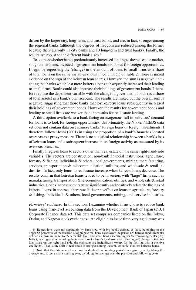
To address whether banks predominantly increased lending to the real estate market,sought other loans, invested in government bonds, or looked for foreign opportunities,I begin by regressing the (change) in the amount of loans to small firms as a shareof total loans on the same variables shown in column (1) of Table 2. There is mixedevidence on the sign of the keiretsu loan shares. However, the sum is negative, indi-cating that banks which lost more keiretsu loans subsequently increased their lendingto small firms. Banks could also increase their holdings of government bonds. I there-fore replace the dependent variable with the change in government bonds (as a shareof total assets) in a bank’s own account. The results are mixed but the overall sum isnegative, suggesting that those banks that lost keiretsu loans subsequently increasedtheir holdings of government bonds. However, the results for government bonds andlending to small firms are weaker than the results for real estate lending.

A third option available to a bank facing an exogenous fall in keiretsus’ demandfor loans is to look for foreign opportunities. Unfortunately, the Nikkei NEEDS dataset does not contain data on Japanese banks’ foreign loans or foreign investments. Itherefore follow Hoshi (2001) in using the proportion of a bank’s branches locatedoverseas as a proxy measure. There is no statistical relationship between a bank’s lossof keiretsu loans and a subsequent increase in its foreign activity as measured by itsoverseas branches.

Finally I regress loans to sectors other than real estate on the same right-hand-sidevariables. The sectors are construction, non-bank financial institutions, agriculture,forestry & fishing, individuals & others, local governments, mining, manufacturing,services, transportation & telecommunication, utilities, and wholesale & retail in-dustries. In fact, only loans to real estate increase when keiretsu loans decrease. Theresults confirm that keiretsu loans tended to be in sectors with “large” firms such asmanufacturing, transportation & telecommunication, utilities, and wholesale & retailindustries. Loans in these sectors were significantly and positively related to the lags ofkeiretsu loans. In contrast, there was little or no effect on loans in agriculture, forestry& fishing, individuals & others, local governments, mining, and service industries.

Firm-level evidence. In this section, I examine whether firms chose to reduce bankloans using firm-level accounting data from the Development Bank of Japan (DBJ)Corporate Finance data set. This data set comprises companies listed on the Tokyo,Osaka, and Nagoya stock exchanges.7 An eligible-to-issue time-varying dummy was

6. Regressions were run separately by bank size, with big banks defined as those belonging to theupper 85 percentile of the fraction of aggregate real bank assets over the period (23 banks), medium banksdefined as those in the 60 to 85 percentile (37), and small banks accounting for the remaining banks (90).In fact, in a regression including the interaction of a bank’s total assets with the (lagged) change in keiretsuloan share on the right-hand side, the estimates are insignificant except for the first lag with a positivecoefficient. That is, the shift to real estate is stronger among the smaller banks that lost keiretsu loans.

7. Note that the data were cleaned up for duplicate accounting periods in a given year by taking theaverage and, if there was a missing year, by taking the average over the previous and following years.


TABLE 3

BOND ISSUANCE ELIGIBILITY FOR DOMESTIC SECURED CONVERTIBLE BONDS

1976 1977 1978 1979 1980 1981 1982 1983 1984 1985 1986 1987 1988 1989 1990

Number ofcompanieseligible

65 378 422 496 559 616 671 675 727 799 819 855 1,084 1,247 1,374

As a share of totalcompanies (in %)

21.5 25.0 27.3 31.8 35.5 38.6 41.3 41.1 43.9 47.9 49.0 51.7 63.4 68.2 71.7

NOTE: The figures are from author’s calculations based on the accounting criteria effective in Japan from October 1976 to December 1990.These criteria are given in Table A3. The underlying accounting data comes from the DBJ Corporate Finance Data Set for listed Japanesecompanies. Therefore, “total companies” refers to the entire sample of companies with accounting data available in a given year. Note thatconvertible bonds were the principle source of public debt financing during the 1980s and these criteria were also applied to foreign issues ofconvertible bonds (refer to Hoshi, Kashyap, and Scharfstein 1993).

created based on the bond issuance criteria (BIC) reported in Table A3. Table 3 reportsthe number of companies eligible to issue secured convertible bonds for each yearfrom 1976 to 1990. The number steadily increased from a low of 65 companies in1976 (0.22 of the total listed) to 1374 by 1990 (0.72 of the total listed). The top panelof Table 4 summarizes the average ratio of a firm’s bank debt to its total bank andbond debt according to whether a firm was eligible to issue bonds or not. I use the termeligible to refer to those firms that later became eligible to issue convertible bondsthroughout the 1982–89 period, following Hoshi et al. (1993). In 1975 (the base year)when credit was still rationed, both eligible and ineligible firms had a bank debt ratioof approximately 0.89. By 1982, this ratio was 0.686 for eligible firms and remained0.888 for ineligible firms. By 1989, the ratio was 0.426 for eligible firms and 0.757for ineligible firms. It therefore appears that firms greatly reduced their dependenceon bank debt upon qualifying to issue bonds.

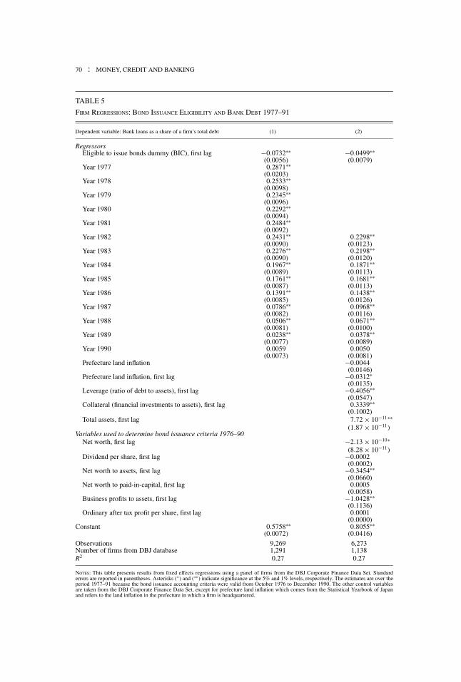
More formal results are reported in Table 5, column (1). The dependent variableis a firm’s bank debt to its total debt. The estimation is an unbalanced panel fixedeffects from 1977 to 1991 for 1291 companies. The ratio of bank debt is regressedon the first lag of the eligible-to-issue dummy and year dummies. The eligibilitydummy is significant at the 1% level and suggests that when a firm becomes eligibleto issue, its share of bank debt falls by 0.07. Column (2) controls for other variablesthat a priori may be thought to affect the bank debt ratio such as firm accountingvariables (leverage, collateral, total assets, and all the separate accounting variablesused to determine bond issuance eligibility) and land inflation in the firm’s prefecture.The latter is included to control for the possibility that high land inflation may be ameasure of good opportunities in the prefecture’s real estate. If so, firms located in thatprefecture would experience a fall in their bank debt if their banks shifted lending toreal estate. The coefficient remains significant at the 1% level, although it is reducedto 0.05.8

8. Note that these results are conservative because many firms reported bond data as missing insteadof zero in the DBJ database. When missing observations were replaced with zero, the results imply thatthe ratio of bank loans falls by approximately 0.10 once a firm qualifies to issue bonds. The magnitude isrobust to the specification in column (2). Refer to the author’s website for these results.

NADA MORA : 69

TAB

LE

4

RA

TIO

OF

FIR

MS’

BA

NK

DE

BT

TO

TOT

AL

DE

BT

1976

1977

1978

1979

1980

1981

1982

1983

1984

1985

1986

1987

1988

1989

1990

By

elig

ibil

ity

tois

sue

conv

erti

ble

bond

sth

roug

hout

1982

–89

Inel

igib

leto

issu

e89

.389

.388

.086

.987

.688

.288

.887

.585

.985

.384

.881

.478

.375

.774

.4Pa

rtly

elig

ible

93.2

91.2

85.6

82.9

82.0

83.6

82.3

80.8

78.1

73.5

70.4

66.0

63.0

60.5

57.7

Elig

ible

88.3

84.9

74.6

70.9

69.4

71.2

68.6

66.1

59.3

56.8

53.8

46.5

43.6

42.6

40.7

By

econ

omic

sect

orR

eale

stat

e93

.889

.189

.189

.089

.289

.387

.688

.379

.984

.784

.880

.367

.971

.672

.6R

eale

stat

e&

cons

truc

tion

94.0

91.2

90.2

88.5

87.8

89.7

88.4

89.2

85.4

87.3

78.5

68.9

63.1

67.8

68.6

Man

ufac

turi

ng88

.584

.780

.075

.975

.577

.474

.872

.066

.662

.359

.354

.451

.550

.449

.1A

mon

gfir

ms

elig

ible

tois

sue

bond

sth

roug

hout

1982

–89

Rea

lest

ate

92.3

92.9

89.8

89.2

85.9

84.3

82.3

84.2

74.2

81.6

76.2

72.5

59.8

64.1

66.1

Rea

lest

ate

&co

nstr

uctio

n91

.790

.688

.186

.384

.385

.983

.485

.079

.484

.670

.157

.651

.856

.555

.8M

anuf

actu

ring

84.9

79.2

71.4

66.3

66.3

67.9

64.0

61.2

53.3

50.0

46.8

39.7

37.0

37.2

36.2

NO

TE:

The

figur

esar

efr

omau

thor

’sca

lcul

atio

nsus

ing

the

DB

JC

orpo

rate

Fina

nce

Dat

aset

for

liste

dno

n-fin

anci

alco

mpa

nies

bycl

assi

fyin

gco

mpa

nies

acco

rdin

gto

elig

ibili

tyto

issu

edu

ring

the

peri

odfr

om19

82to

1989

and

acco

rdin

gto

whi

chse

ctor

they

belo

nged

.Elig

ible

-to-

issu

ebo

ndcr

iteri

aar

esh

own

inTa

ble

A3.

Afir

m’s

tota

ldeb

tis

calc

ulat

edas

the

sum

ofou

tsta

ndin

gsh

ort-

term

bank

loan

s(D

BJ

code

K19

60)+

long

-ter

mba

nklo

ans

(K23

50)+

tota

lout

stan

ding

bond

sco

mpo

sed

ofst

raig

htbo

nds

(K68

50),

conv

ertib

lebo

nds

(K68

90),

and

war

rant

bond

s(K

6930

).A

firm

’sba

nkde

btra

tiois

then

calc

ulat

edas

the

ratio

ofits

shor

t-te

rman

dlo

ng-t

erm

bank

loan

sto

itsto

tald

ebt.

The

calc

ulat

ions

are

base

don

allc

ompa

nies

with

acco

untin

gda

taav

aila

ble

for

each

year

duri

ng19

82–8

9(r

esul

ting

in37

1co

mpa

nies

).R

efer

toTa

ble

3fo

rin

form

atio

non

com

pani

esel

igib

leto

issu

ebo

nds

(dom

estic

secu

red

conv

ertib

le)

duri

ngth

epe

riod

.


TABLE 5

FIRM REGRESSIONS: BOND ISSUANCE ELIGIBILITY AND BANK DEBT 1977–91

Dependent variable: Bank loans as a share of a firm’s total debt (1) (2)

RegressorsEligible to issue bonds dummy (BIC), first lag −0.0732∗∗ −0.0499∗∗

(0.0056) (0.0079)Year 1977 0.2871∗∗

(0.0203)Year 1978 0.2533∗∗

(0.0098)Year 1979 0.2345∗∗

(0.0096)Year 1980 0.2292∗∗

(0.0094)Year 1981 0.2484∗∗

(0.0092)Year 1982 0.2431∗∗ 0.2298∗∗

(0.0090) (0.0123)Year 1983 0.2276∗∗ 0.2198∗∗

(0.0090) (0.0120)Year 1984 0.1967∗∗ 0.1871∗∗

(0.0089) (0.0113)Year 1985 0.1761∗∗ 0.1681∗∗

(0.0087) (0.0113)Year 1986 0.1391∗∗ 0.1438∗∗

(0.0085) (0.0126)Year 1987 0.0786∗∗ 0.0968∗∗

(0.0082) (0.0116)Year 1988 0.0506∗∗ 0.0671∗∗

(0.0081) (0.0100)Year 1989 0.0238∗∗ 0.0378∗∗

(0.0077) (0.0089)Year 1990 0.0059 0.0050

(0.0073) (0.0081)Prefecture land inflation −0.0044

(0.0146)Prefecture land inflation, first lag −0.0312∗

(0.0135)Leverage (ratio of debt to assets), first lag −0.4056∗∗

(0.0547)Collateral (financial investments to assets), first lag 0.3339∗∗

(0.1002)Total assets, first lag 7.72 × 10−11∗∗

(1.87 × 10−11)Variables used to determine bond issuance criteria 1976–90

Net worth, first lag −2.13 × 10−10∗(8.28 × 10−11)

Dividend per share, first lag −0.0002(0.0002)

Net worth to assets, first lag −0.3454∗∗(0.0660)

Net worth to paid-in-capital, first lag 0.0005(0.0058)

Business profits to assets, first lag −1.0428∗∗(0.1136)

Ordinary after tax profit per share, first lag 0.0001(0.0000)

Constant 0.5758∗∗ 0.8055∗∗(0.0072) (0.0416)

Observations 9,269 6,273Number of firms from DBJ database 1,291 1,138R2 0.27 0.27

NOTES: This table presents results from fixed effects regressions using a panel of firms from the DBJ Corporate Finance Data Set. Standarderrors are reported in parentheses. Asterisks (∗) and (∗∗) indicate significance at the 5% and 1% levels, respectively. The estimates are over theperiod 1977–91 because the bond issuance accounting criteria were valid from October 1976 to December 1990. The other control variablesare taken from the DBJ Corporate Finance Data Set, except for prefecture land inflation which comes from the Statistical Yearbook of Japanand refers to the land inflation in the prefecture in which a firm is headquartered.

NADA MORA : 71

Evidence from the DBJ database is also consistent with the flow of funds figuresto real estate reported in Table 1. The lower panel of Table 4 reports the ratio of afirm’s bank debt to total debt for firms in the real estate, real estate & construction,and manufacturing sector for comparison. The share of bank debt in 1976 is around0.94 for real estate firms and 0.89 for manufacturing firms. By 1986, the share haddeclined to 0.59 for manufacturing firms but only to 0.85 for real estate firms. Evenby 1990 and at the peak of the boom, the major part of real estate firms’ debt wasowed to banks (0.73, and 0.66 among the subset of real estate firms fully eligible toissue bonds throughout the 1982–89 period). Therefore the evidence suggests thatlarge real estate companies with the ability to borrow in the bond market were notfueling the boom. Bank lending remained the dominant means of financing real estateinvestment during the 1980s, even for relatively large companies. The DBJ databaseis composed of large companies as they are listed on Japan’s major stock exchanges.The results would likely be even more pronounced if data were available on financingof smaller real estate companies.9

2. SHOCKS TO THE SUPPLY OF BANK CREDIT: IS THEREAN EFFECT ON LAND PRICES?

This section uses bank loans to keiretsu firms to instrument for the supply of realestate loans in order to determine whether bank credit influences land prices. Thequestion is assessed by taking both cross-sectional and time-series’ slices of the dataon Japan’s 47 prefectures. To briefly review the theory for potential causality runningfrom bank credit to asset prices, in the presence of credit constraints, credit limitsare affected by the price of assets used as collateral for loans. However, the extentto which banks are willing to finance projects that require the acquisition of assetsalso matters. Asset prices can be positively affected by slackened credit limits and anincrease in available liquidity.

2.1 Empirical Estimation

Balance sheet data on 150 banks were compiled from the Nikkei NEEDS database.These data were used in Section 1.2 when testing the HK hypothesis. The variablesof interest in this section include loans disaggregated by sector (e.g., real estate),loans to keiretsu and listed firms, and the location of a bank’s headquarters. Theindividual bank data are then aggregated by prefecture. Table A2 presents samplesummary statistics. The maximum sample of the data is from 1976 to 1998. Howeverthe effective sample is from 1981 to 1993 because prefecture land prices are availablebeginning in 1980 and keiretsu loan numbers end in 1993. This is not constrainingbecause the 1981–93 sample is the relevant period to study the real estate boom.

9. The Ministry of Finance provides data on its website under the heading “Financial Statement Statisticsof Corporations by Industry, Quarterly” which include unlisted and smaller companies. However, data onfirm financing are only provided by size distribution for the following aggregate categories: all industry,manufacturing, and non-manufacturing.


FIG. 3. Inflation (a) Land Price Inflation and the Nikkei Stock Market Index, (b) Prefecture-Level Land Price Inflation(Selected Prefectures).

NOTES: Source: The Nikkei index (Nikkei Stock Average, TSE 225 issues, end of month) is from the Bank of Japan,http://www.boj.or.jp/en. Land prices, all areas and six largest cities are from the Japan Statistical Yearbook’s Table 17–12Index of Urban Land Prices (1960–2003), which in turn are from the Japan Real Estate Institute (as of end of March).Prefecture land prices are from the Japan Statistical Yearbook, various issues, which come from the annual July 1stPrefectural Land Price Survey carried out by the Land and Water Bureau, Ministry of Land, Infrastructure and Transport.The weighted average over six categories of land is taken: residential site, prospective housing land, commercial site,quasi-industrial site, industrial site, and housing land within urbanization control area. Land price indices are divided bythe GDP deflator to obtain real land prices, then the inflation rate is calculated as the annual log difference.

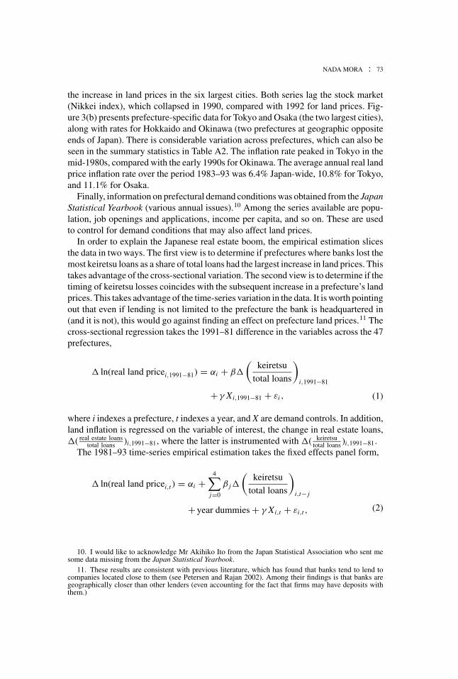
Land price data are available from the annual prefectural land price survey, con-ducted by the Ministry of Land, Infrastructure, and Transport on Japan’s 47 prefecturesand reported in the Japan Statistical Yearbook. Figure 3 shows real land price inflationfigures, which are expressed as annual rates. Averages for the country and the largestsix cities are presented in Figure 3(a). It is interesting that the country average lags

NADA MORA : 73

the increase in land prices in the six largest cities. Both series lag the stock market(Nikkei index), which collapsed in 1990, compared with 1992 for land prices. Fig-ure 3(b) presents prefecture-specific data for Tokyo and Osaka (the two largest cities),along with rates for Hokkaido and Okinawa (two prefectures at geographic oppositeends of Japan). There is considerable variation across prefectures, which can also beseen in the summary statistics in Table A2. The inflation rate peaked in Tokyo in themid-1980s, compared with the early 1990s for Okinawa. The average annual real landprice inflation rate over the period 1983–93 was 6.4% Japan-wide, 10.8% for Tokyo,and 11.1% for Osaka.

Finally, information on prefectural demand conditions was obtained from the JapanStatistical Yearbook (various annual issues).10 Among the series available are popu-lation, job openings and applications, income per capita, and so on. These are usedto control for demand conditions that may also affect land prices.

In order to explain the Japanese real estate boom, the empirical estimation slicesthe data in two ways. The first view is to determine if prefectures where banks lost themost keiretsu loans as a share of total loans had the largest increase in land prices. Thistakes advantage of the cross-sectional variation. The second view is to determine if thetiming of keiretsu losses coincides with the subsequent increase in a prefecture’s landprices. This takes advantage of the time-series variation in the data. It is worth pointingout that even if lending is not limited to the prefecture the bank is headquartered in(and it is not), this would go against finding an effect on prefecture land prices.11 Thecross-sectional regression takes the 1991–81 difference in the variables across the 47prefectures,

� ln(real land pricei,1991−81) = αi + β�

(keiretsu

total loans

)i,1991−81

+ γ Xi,1991−81 + εi , (1)

where i indexes a prefecture, t indexes a year, and X are demand controls. In addition,land inflation is regressed on the variable of interest, the change in real estate loans,�( real estate loans

total loans )i,1991−81, where the latter is instrumented with �( keiretsutotal loans )i,1991−81.

The 1981–93 time-series empirical estimation takes the fixed effects panel form,

� ln(real land pricei,t ) = αi +4∑

j=0

β j�

(keiretsu

total loans

)i,t− j

+ year dummies + γ Xi,t + εi,t , (2)

10. I would like to acknowledge Mr Akihiko Ito from the Japan Statistical Association who sent mesome data missing from the Japan Statistical Yearbook.

11. These results are consistent with previous literature, which has found that banks tend to lend tocompanies located close to them (see Petersen and Rajan 2002). Among their findings is that banks aregeographically closer than other lenders (even accounting for the fact that firms may have deposits withthem.)


� ln(real land pricei,t ) = αi + β�

(real estate loans

total loans

)i,t

+ year dummies + γ Xi,t + εi,t , (3)

where i indexes a prefecture, t indexes a year, X are demand controls, and�( real estate loans

total loans )i,t is instrumented with �( keiretsutotal loans )i,t and its four lags.12 Note that

the dependent variable, land price inflation, is expressed as an annual rate comparedwith the cross-section regressions, in which inflation is expressed as the rate over the1981–91 period.

2.2 Results

Table 6 reports the results of the cross-section regression, equation (1). For a 0.01decrease in the share of keiretsu loans to total loans in a prefecture, land inflationincreases by 4.7% (column (1)). This result is significant at the 1% level. Note thatthe average share of keiretsu loans is 0.06 during the estimated sample. Column (3)reports the instrumental variable (IV) results when instrumenting for the real estateloan share with the keiretsu loan share. The estimate is 20.3% and is significantat the 1% level. This suggests that prefectures whose banks experienced a greaterloss in their proportion of keiretsu loans experienced a larger increase in real estatelending, which fueled land inflation.13 Column (5) repeats the analysis but for “risky”loans instead of real estate loans. Risky loans are defined as the sum of real estate,construction, and non-bank financial institution loans, which were used to proxy forrisky loans by Hoshi (2001). As discussed in Section 1.2, a major part of non-bankfinancial institutions were the “jusen,” which were housing loan subsidiaries of banks.Similar results are obtained: a 0.01 increase in the instrumented share of risky loansleads to 14.2% higher prefectural land inflation over the 1981–91 period.

It is interesting to contrast the ordinary least squares (OLS) results to the IV results.Column (2) presents the regression of prefectural land inflation on a prefecture’sdifference in its real estate loan share over the 1981–91 period. Because the latteris not instrumented, the estimate of 11.5% higher inflation should be interpreted asa correlation. It is interesting that IV estimation implies an effect (20.3%) almost

12. Note that the variables for keiretsu loans and real estate loans are taken as a proportion of totalloans. This is the approach taken by Hoshi (2001). The advantage compared with using growth rates isthat the latter can exaggerate the importance of keiretsu loans if a bank starts from a low level. However,the conjecture that the significant effect of keiretsu loans on real estate loans may stem directly from theconstruction of the variables is not the case. First, the “total loans” measure used to normalize real estateloans comes from summing the 12 components of reported sectoral loans. In contrast, the “total loans”used for keiretsus comes from the total loans measure in a bank’s balance sheet. More importantly, nomechanical relation was found when robustness checks were done on other sectoral loans regressed onthe keiretsu loans. In fact, and as discussed in Section 1.2, only loans to real estate increase when keiretsuloans decrease.

13. The regressions were also estimated excluding the Tokyo and Osaka prefectures. This is to counterthe criticism that the coefficients might simply be capturing that the two largest prefectures had high landinflation rates (for some other reason) coupled with a larger share of loans to keiretsu firms. However, theresults remain significant.

NADA MORA : 75

TAB

LE

6

TH

EE

FFE

CT

OF

BA

NK

CR

ED

ITO

NL

AN

DPR

ICE

S:T

HE

PRE

FEC

TU

RE

CR

OSS

-SE

CT

ION

AL

VIE

W

Dep

ende

ntva

riab

le:L

ogdi

ffer

ence

inre

alpr

efec

tura

lla

ndpr

ice

betw

een

1991

and

1981

(1)

(2)

(3)

(4)

(5)

(6)

(7)

(8)

All

regr

esso

rsar

eth

edi

ffere

nce

betw

een

1991

and

1981

a

Kei

rets

ulo

ansh

are

−4.6

568∗∗

−3.4

475∗∗

(0.7

352)

(0.9

895)

Rea

lest

ate

loan

shar

e11

.485

2∗∗20

.301

6∗∗14

.864

9∗∗(2

.167

2)(4

.612

3)(4

.898

9)“R

isky

”lo

ansh

are

(loa

nsto

real

esta

te4.

4586

∗14

.248

9∗∗13

.543

5&

cons

truc

tion

&no

n-ba

nk(1

.663

2)(5

.013

0)(7

.521

4)fin

anci

alin

stitu

tions

)M

acro

cont

rols

c

Pref

ectu

repo

pula

tion,

inlo

gs3.

6120

∗∗0.

8910

3.88

69(0

.988

3)(1

.319

7)(2

.187

5)Pr

efec

ture

unem

ploy

men

trat

e−0

.137

60.

0878

0.00

19(0

.194

0)(0

.218

3)(0

.348

4)Pr

efec

ture

inco

me

per

capi

ta,i

nlo

gs−0

.099

41.

1116

−2.9

717

(0.7

785)

(0.9

088)

(3.1

228)

Pref

ectu

rejo

bop

enin

gsto

appl

icat

ions

−0.2

670

−0.2

694

−0.0

069

(0.1

415)

(0.1

740)

(0.3

522)

Pref

ectu

reC

PIex

clud

ing

rent

,in

logs

0.39

254.

0841

−3.1

615

(3.3

966)

(2.7

428)

(8.1

607)

Inst

rum

enti

ngfo

rre

ales

tate

or“

risk

y”Y

esY

esY

esY

eslo

ansh

are

wit

hke

iret

sulo

ansh

are?

Con

stan

t0.

8961

∗∗0.

7439

∗∗0.

5197

∗∗0.

6749

∗∗−0

.118

01.

0232

−0.5

199

1.83

71(0

.054

7)(0

.064

1)(0

.118

0)(0

.125

2)(0

.410

3)(0

.712

8)(0

.722

9)(2

.011

0)N

umbe

rof

pref

ectu

res

4747

4747

4747

4747

R2

0.35

0.38

0.16

0.17

R2<

0b0.

570.

46R

2<

0b

NO

TE

S:R

obus

tsta

ndar

der

rors

are

repo

rted

inpa

rent

hese

san

dth

eyar

ecl

uste

red

bypr

efec

ture

.Ast

eris

ks(∗

)an

d(∗

∗ )in

dica

tesi

gnifi

canc

eat

the

5%an

d1%

leve

ls,r

espe

ctiv

ely.

aE

xcep

tfor

Pref

ectu

repo

pula

tion

and

unem

ploy

men

t,w

hich

are

the

diff

eren

cebe

twee

n19

90an

d19

80du

eto

data

avai

labi

lity.

bN

ote

that

in2S

LS

the

R2

can

som

etim

esbe

nega

tive,

even

whe

na

cons

tant

isin

clud

ed.

cT

heco

ntro

lsar

eco

mpi

led

from

the

Japa

nSt

atis

tica

lYea

rboo

k,va

riou

sis

sues

.


twice as large. A similar result is found with risky loans. That the coefficient is largerwhen using IV underlies the significance of keiretsu loans in identifying real estatelending and the latter’s independent effect on land prices. One possible explanationis that a higher land price also reduces demand for land, which is the standard resultif we ignore the positive effect on net worth coming from the relaxation of creditconstraints. This biases the OLS coefficient downward. Another possibility is thata higher land price increases people’s expectation of future increases in land prices(especially in a speculative setting). This leads to an increase in supply of land andconstruction, and mitigates the OLS estimate.

Columns (6) through (8) report robustness results by including differences of vari-ables to control for demographic and economic differences across prefectures (suchas job openings to applications, growth in income per capita, population growth,the unemployment rate, and consumer price index (CPI) excluding rent). The (in-strumented) real estate loan share remains significant at the 1% level but its effecton land inflation is now smaller in magnitude (14.9% compared with 20.3% previ-ously). Similarly, the coefficient on the risky loan share is reduced but only to 13.5%.Apart from a prefecture’s population and its job openings to applications ratio, theremaining macroeconomic controls are insignificant. This may be on account of thelimited degrees of freedom and potential multicollinearity. Alternatively, demandfactors may not have been central to the large increase in land inflation over theperiod.

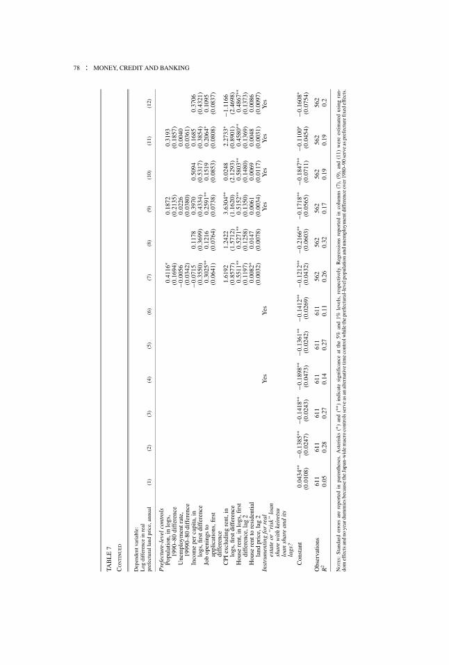
Table 7 reports the results of regressions that take advantage of the time-seriesvariation over the period 1981–93, equations (2) and (3). The first column reports thesimplest regression of the log difference in real prefectural land price regressed on the(first difference of) keiretsu loan share and its four lags, allowing for prefecture fixedeffects. The results are significant and imply that a 0.01 annual decrease (over 5 years)in the share of keiretsu loans to total loans leads to a subsequent 10% increase in aprefecture’s annual land inflation rate. Column (2) includes year dummies. Althoughthe significance and magnitude of the keiretsu loan loss is reduced, it is still the casethat a fall of 0.01 in keiretsu loans leads to a 6% increase in land price inflation.

Column (3) reports the estimates for the simple regression without an instrumentfor the real estate loan share. The results confirm the correlation between the increasein land prices and real estate loans (3.3% higher inflation). Column (4) instrumentsthe contemporaneous real estate loan share with the keiretsu loan share and its fourlags. The coefficient on the real estate loans is much larger and coincides with 27%higher land inflation in a prefecture. However the result is significant only at the 13%level.14 Columns (5) and (6) repeat the analysis for risky loans. A 0.01 increase in theinstrumented risky loan share coincides with a 9.5% higher land inflation rate and issignificant at the 10% level.15

14. It is worth mentioning that the Hausman test for all these models favors random effects over fixedeffects (e.g., the chi-squared value is 0.27 for the model in column (4)). Random effects is more efficientand the coefficient is estimated to be 18.6% and is significant at the 1.2% level. However, fixed effects arereported for ease of understanding the time dimension of the keiretsu shock.

15. The random effects model is favored and results in a similar coefficient estimate of 9.3%, which issignificant at the 1% level.

NADA MORA : 77

TAB

LE

7

TH

EE

FFE

CT

OF

BA

NK

CR

ED

ITO

NL

AN

DPR

ICE

S:T

HE

TIM

E-S

ER

IES

VIE

W:P

RE

FEC

TU

RE

FIX

ED

EFF

EC

TS

1981

–93

Dep

ende

ntva

riab

le:

Log

diff

eren

cein

real

pref

ectu

rall

and

pric

e,an

nual

(1)

(2)

(3)

(4)

(5)

(6)

(7)

(8)

(9)

(10)

(11)

(12)

Reg

ress

ors

Kei

rets

ulo

ansh

are,

first

diff

eren

ce−3

.315

4∗∗−1

.801

9∗∗−1

.164

0∗−1

.644

8∗(0

.659

7)(0

.618

6)(0

.582

1)(0

.671

6)K

eire

tsu

loan

shar

e,fir

stdi

ffer

ence

,lag

1−3

.399

6∗∗−1

.300

2−1

.087

0−1

.134

6(0

.762

6)(0

.727

0)(0

.614

5)(0

.768

6)K

eire

tsu

loan

shar

e,fir

stdi

ffer

ence

,lag

2−2

.438

0∗∗−1

.337

9−1

.394

5∗−1

.518

0(0

.784

1)(0

.753

2)(0

.590

7)(0

.791

3)K

eire

tsu

loan

shar

e,fir

stdi

ffer

ence

,lag

3−0

.959

2−1

.018

4−1

.114

2−1

.208

9(0

.770

0)(0

.734

7)(0

.582

6)(0

.771

8)K

eire

tsu

loan

shar

e,fir

stdi

ffer

ence

,lag

4−0

.197

9−0

.523

2−0

.710

7−0

.597

3(0

.659

4)(0

.616

8)(0

.545

7)(0

.652

7)R

eale

stat

elo

ansh

are,

first

diff

eren

ce3.

3498

∗27

.057

515

.687

6∗17

.300

2(1

.365

1)(1

8.01

39)

(6.5

623)

(15.

6500

)“R

isky

”lo

ansh

are

(loa

nsto

real

esta

te&

cons

truc

tion

&no

n-ba

nkfin

anci

alin

stitu

tions

.)

1.62

21∗

9.46

626.

3942

∗7.

9049

(0.7

119)

(5.0

734)

(2.7

412)

(5.5

950)

Year

dum

mie

s?Y

esY

esY

esY

esY

esY

esY

esY

esJa

pan-

wid

em

acro

cont

rols

Japa

nese

unem

ploy

men

t,fir

stdi

ffer

ence

−0.0

883

−0.0

251

−0.0

682

(0.0

687)

(0.0

824)

(0.0

738)

Nik

keis

tock

mar

ket,

inlo

gs,fi

rstd

iffe

renc

e0.

0344

−0.1

139

−0.0

296

(0.0

656)

(0.0

889)

(0.0

699)

Japa

npo

pula

tion,

inlo

gs,

first

diff

eren

ce12

.864

111

.532

76.

3481

(7.2

285)

(7.9

958)

(8.2

479)

(Con

tinu

ed)


TAB

LE

7

CO

NT

INU

ED

Dep

ende

ntva

riab

le:

Log

diff

eren

cein

real

pref

ectu

rall

and

pric

e,an

nual

(1)

(2)

(3)

(4)

(5)

(6)

(7)

(8)

(9)

(10)

(11)

(12)

Pre

fect

ure-

leve

lcon

trol

sPo

pula

tion,

inlo

gs,

1990

–80

diff

eren

ce0.

4116

∗0.

1872

0.31

93(0

.169

4)(0

.213

5)(0

.185

7)U

nem

ploy

men

trat

e,19

990–

80di

ffer

ence

−0.0

056

0.02

260.

0040

(0.0

342)

(0.0

380)

(0.0

361)

Inco

me

per

capi

ta,i

nlo

gs,fi

rstd

iffe

renc

e−0

.071

50.

1178

0.39

700.

5094

0.16

850.

3706

(0.3

550)

(0.3

699)

(0.4

334)

(0.5

317)

(0.3

854)

(0.4

321)

Job

open

ings

toap

plic

atio

ns,fi

rst

diff

eren

ce

0.30

25∗∗

0.12

160.

2591

∗∗0.

1519

0.20

64∗

0.10

95(0

.064

1)(0

.076

4)(0

.073

8)(0

.085

3)(0

.080

8)(0

.083

7)

CPI

excl

udin

gre

nt,i

nlo

gs,fi

rstd

iffe

renc

e1.

6192

1.24

223.

6304

∗∗0.

0248

2.27

33∗

−1.1

166

(0.8

577)

(1.5

712)

(1.1

620)

(2.1

293)

(0.8

901)

(2.4

698)

Hou

sere

nt,i

nlo

gs,fi

rst

diff

eren

ce,l

ag2

0.55

11∗∗

0.52

71∗∗

0.51

52∗∗

0.58

03∗∗

0.45

80∗∗

0.48

67∗∗

(0.1

197)

(0.1

258)

(0.1

350)

(0.1

480)

(0.1

369)

(0.1

373)

Hou

sere

ntto

resi

dent

ial

land

pric

e,la

g2

0.00

82∗

0.01

470.

0061

0.00

690.

0048

0.00

86(0

.003

2)(0

.007

8)(0

.003

4)(0

.011

7)(0

.003

1)(0

.009

7)In

stru

men

ting

for

real

esta

teor

“ri

sk”

loan

shar

ew

ith

keir

etsu

loan

shar

ean

dit

sla

gs?

Yes

Yes

Yes

Yes

Yes

Yes

Con

stan

t0.

0434

∗∗−0

.138

5∗∗−0

.141

8∗∗−0

.189

8∗∗−0

.136

1∗∗−0

.141

2∗∗−0

.121

2∗∗−0

.216

6∗∗−0

.171

8∗∗−0

.184

7∗∗−0

.110

0∗−0

.160

8∗(0

.010

8)(0

.024

7)(0

.024

3)(0

.047

3)(0

.024

2)(0

.026

9)(0

.043

2)(0

.060

3)(0

.056

5)(0

.071

1)(0

.045

4)(0

.075

4)

Obs

erva

tions

611

611

611

611

611

611

562

562

562

562

562

562

R2

0.05

0.28

0.27

0.14

0.27

0.11

0.26

0.32

0.17

0.19

0.19

0.2

NO

TE

S:St

anda

rder

rors

are

repo

rted

inpa

rent

hese

s.A

ster

isks

(∗)

and

(∗∗ )

indi

cate

sign

ifica

nce

atth

e5%

and

1%le

vels

,re

spec

tivel

y.R

egre

ssio

nsre

port

edin

colu

mns

(7),

(9),

and

(11)

wer

ees

timat

edus

ing

ran-

dom

effe

ctsa

ndno

year

dum

mie

sbec

ause

the

Japa

n-w

ide

mac

roco

ntro

lsse

rve

asan

alte

rnat

ive

time

cont

rolw

hile

the

pref

ectu

ral-

leve

lpop

ulat

ion

and

unem

ploy

men

tdif

fere

nce

over

1980

–90

serv

eas

pref

ectu

refix

edef

fect

s.

NADA MORA : 79

Finally, demand controls are included in the regressions reported in columns (7)through (12). As in the cross-section regressions, prefecture-level controls are in-cluded (job openings to applications, growth in income per capita, population growth,the unemployment rate, CPI excluding rent, as well as the second lags of house rentand the ratio of rent to residential land price). Japan-wide macro controls are alsoincluded (changes in the unemployment rate, equity prices, and population). Many ofthese variables enter with the expected sign. For example, a larger growth in a prefec-ture’s population contributes to higher land inflation. A prefecture experiencing anincrease in its job openings to applications ratio has higher land inflation, etc. What isimportant is that the significance of the loss in keiretsu loans is robust to these changes:a 0.01 annual decrease in the share (over 5 years) contributes to approximately 6%higher land inflation. Note that this estimate is similar to that found in column (2),which only includes year dummies. The result is similar whether we look at column(7) or (8). Column (7) reports a random effects model because some of the prefecturecontrols are time independent and therefore do not allow for prefecture fixed effects.Also omitted are the year dummies because the Japan-level controls are only timevarying with no cross-sectional variation.

Columns (9) and (10) show the IV regression for real estate loans reported incolumn (4) but re-estimated with demand controls. The magnitude is reduced to15.7–17.3% higher inflation. The coefficient of 17.3% from the fixed effects modelis not significant (in column (4) it was only significant at the 13% level). However,the associated random effects coefficient is 20.9% and is significant at the 5% level(the Hausman test chi-squared is 1.26 favoring the random effects model). Finally,columns (11) and (12) add demand controls to the IV regression for risky loansreported in column (6). The coefficient of 7.9% from the fixed effect model is onlysignificant at the 16% level, while the random effects coefficient for the same modelis 9.5% (similar to that reported in column (6)) and is significant at the 1.3% level.

From the panel regressions, it is evident that the timing of the keiretsu losses gen-erally coincides with subsequent increases in land prices in a prefecture during theperiod from 1981 to 1993. A 0.01 increase in a prefecture’s instrumented real estateloan share corresponds to a 15–27% higher annual land inflation rate (and is sig-nificant for the Hausman preferred random effects model). More generally, a 0.01instrumented increase in a prefecture’s risky loan share (loans to real estate, con-struction and non-bank financial institutions) leads to a 6–9.5% higher land inflationrate.

To get a better sense of the magnitude of the implied effect, it is worth comparingestimates with actual figures for Japan during the period from 1983 to 1993. Theaverage over Japan’s 47 prefectures of the share of keiretsu loans was 0.06, of realestates loans was 0.08, and of “risky” loans was 0.21. As for changes in these shares,the average for keiretsu loans was −0.002, for real estate loans was 0.002, and for“risky” loans was 0.007. At the same time, the average annual real land inflation ratein Japan was 6.4%. A simple calculation combining the coefficient estimates frommodel 7.3 (i.e., the one reported in Table 7, column (3)) and these average figures,implies that the average increase in real estate loans of 0.002 would lead to an increase


FIG. 4. The Japan Average Actual Land Inflation Rate and the Predicted Rate.

NOTES: Source: Land inflation is the average over the 47 prefectures of the prefectural real land price inflation. The predictedinflation rate comes from Model 7.3 for the uninstrumented real estate loans and from Model 7.4 for the keiretsu-shareinstrumented real estate loans (refer to columns (3) and (4) in Table 7).

in inflation of 0.8%. When using the IV coefficients from model 7.4, however, theimplied inflation rate coming from real estate lending is 6.18%, almost identical tothe actual figure in Japan over the period. A figure of 6.17% is derived from riskylending from model 7.6. Looking specifically at Tokyo, the implied inflation rate frommodel 7.4 is 16.6%, higher than the average actual inflation rate of 10.8%. Overallthese results suggest a large but not unrealistic effect of bank credit on land prices.

Figure 4 shows the time variation in the Japan-wide average land inflation rate andthe predicted rates based on the simple regression using real estate loans (model 7.3)and on the instrumented real estate loans (model 7.4). The instrumented real estatelending by banks predicts the actual land inflation rate well (this is also the casefor risky loans) and particularly during the 1980s, which is the relevant period. Thepredicted component tends to lead the actual rate during the boom. Note that thepredicted land inflation coming from the uninstrumented real estate lending does notdo a good job at capturing the actual path of land inflation.

3. CONCLUSION

Japan deregulated its financial system in the 1980s. The regulatory change thatdecreased the demand for loans by keiretsus led banks to increase lending in the realestate sector. I find evidence consistent with this explanation for the real estate boom.There is no support for the alternative that real estate had (or was perceived to have)good opportunities, rationalizing a shift of bank lending to real estate.

The Japanese real estate boom during the 1980s therefore provides the appropriatesetting and some answers to the question of whether bank credit affects asset prices. I

NADA MORA : 81

use a bank’s loss of keiretsu loans as an instrument for the supply of real estate loans,and take advantage of both the cross-sectional and time-series variation in land pricesin Japan’s 47 prefectures. The main findings are twofold: First, a 0.01 increase in aprefecture’s instrumented real estate loans as a share of total loans causes 14–20%higher land inflation over the 1981–91 period. Second, the timing of keiretsu loanlosses coincides with subsequent land inflation in a prefecture. In short, shocks to thesupply of credit fuel land prices.

That the supply of credit can have such a considerable impact on asset prices hasimplications for both monetary and regulatory policy. If there were no imperfectionsin credit markets, banks’ willingness to offer loans would have no impact on assetprices. The latter would only depend on the discounted flow of future income derivingfrom the asset. But in the presence of credit constraints and in the short run, a shock likeincomplete financial deregulation can have an amplified effect on asset prices. Thiscan be true even if financial liberalization were to ease credit market imperfectionsin the long run. The case of Japan illustrates this. Japan underwent incomplete andslow financial deregulation over two decades. The resulting “over-banking” problem(as dubbed by Hoshi and Kashyap) which has characterized the Japanese bankingsystem is gradually being resolved as banks merge and shrink.

What lessons for monetary and regulatory policy can be drawn? If the processof liberalization in Japan had been faster and more complete, the wrong incentiveswould not have materialized to cause banks to shift lending disproportionately to realestate. Ito (2004) argues that the supervisory regime should have been strengthenedin the 1980s to ensure stricter prudential guidelines (on real estate lending) when theregulatory regime began to allow for more competition. With the benefit of hindsight,such a move would have been justified. That said, central banks continue to strug-gle with appropriate policy when there is asset price inflation and little goods priceinflation. For example, Bernanke and Gertler (2001) argue that central banks shouldrespond to asset prices only to the extent to which they influence expected inflation.More research is needed, but the results of this paper suggest that banks can activelycontribute to asset price inflation.

APPENDIX

Financial Regulation and Deregulation in Japan

Banks and households. The Japanese economy was characterized by interest ratecontrols (TIRAL), which were effective from 1947 until 1992. While these werecontrols on deposit rates, they were accompanied by loan rate restrictions to ensure thatlong-term credit banks earned profits. Certain implications of interest rate controls onbanks’ profitability have been highlighted by Hoshi and Kashyap (2001) and Kitagawaand Kurosawa (1994). Hoshi and Kashyap argue that the increase in fraction of assetslent out by banks during deregulation reflects their attempting to make up throughvolume the reduction in margins they received on loans. Kitagawa and Kurosawa echothis view that the objective of banks was not profit but scale and that the two may have


TAB

LE

A1

SAM

PLE

STA

TIS

TIC

S:19

81–9

1,A

CR

OSS

BA

NK

S

Mea

n

Pane

lof

150

bank

s19

81–9

119

8119

91St

d.de

v.M

inim

umM

axim

um

Kei

rets

ulo

ans,

assh

are

ofto

tal

0.06

900.

1246

0.03

990.

1714

0.00

001.

7649

5a

Firs

tdif

fere

nce

−0.0

076

0.00

120.

0029

0.04

26−0

.499

70.

3238

Rea

lest

ate

loan

s,as

shar

eof

tota

l0.

0853

0.06

320.

0973

0.05

280.

0000

0.34

87Fi

rstd

iffe

renc

e0.

0032

0.00

09−0

.013

60.

0112

−0.0

474

0.09

33R

ealg

row

thra

teof

real

esta

telo

ans

0.10

580.

0262

0.01

600.

1180

−0.2

921

0.86

05(I

nter

esto

nlo

ans

&di

scou

nts

–In

tere

ston

depo

sits

)/to

tala

sset

s0.

0089

0.00

520.

0069

0.00

66−0

.018

70.

0397

Net

inte

rest

inco

me/

tota

lass

ets

0.01

800.

0100

0.01

490.

0064

−0.0

028

0.03

09In

tere

stin

com

eon

loan

s/to

tall

oans

0.06

230.

0411

0.07

310.

0117

0.00

000.

1081

Inte

rest

expe

nse

onde

posi

ts/to

tald

epos

its0.

0387

0.02

690.

0506

0.01

090.

0008

0.10

05Fi

rstd

iffe

renc

e0.

0028

0.00

750.

0162

0.00

95−0

.032

70.

0577

Am

ount

oflo

ans

tosm

allb

orro

wer

s/to

tall

oans

0.85

970.

9382

0.86

270.

2239

0.00

002.

2019

Gov

ernm

entb

onds

inow

nac

coun

t/tot

alas

sets

0.04

990.

0539

0.05

110.

0228

0.00

730.

1496

Fore

ign

bran

ches

/tota

lbra

nche

s0.

0145

0.01

180.

0187

0.05

940.

0000

0.61

90To

tala

sset

s,in

mill

ion

yen

3755

744

1954

148

6067

036

8365

080

5440

966

6000

00To

tala

sset

s,re

alte

rms

3989

423

291

6030

987

065

648

6767

36To

tall

oans

,in

mill

ion

yen

1860

464

8864

7332

2430

740

2569

529

878

3590

0000

Sect

oral

shar

es:

Ris

kylo

ans

(rea

lest

ate

&co

nstr

uctio

n&

non-

bank

sfin

anci

alin

stitu

tions

)0.

2209

0.17

230.

2539

0.07

270.

0000

0.51

72Fi

rstd

iffe

renc

e0.

0078

0.00

45−0

.013

70.

0167

−0.0

717

0.14

76L

oans

toA

gric

ultu

re,F

ores

try

and

Fish

ery

0.01

020.

0117

0.00

840.

0091

0.00

000.

0472

Loa

nsto

Indi

vidu

als

&O

ther

s0.

1699

0.16

730.

2000

0.05

010.

0664

0.39

95L

oans

toL

ocal

Gov

ernm

ents

0.01

420.

0162

0.00

960.

0187

0.00

000.

1099

Loa

nsto

Min

ing

0.00

390.

0043

0.00

320.

0037

0.00

000.

0329

Loa

nsto

Man

ufac

turi

ng0.

1975

0.23

940.

1571

0.07

220.

0371

0.41

48L

oans

toSe

rvic

es0.

1175

0.08

900.

1401

0.04

030.

0000

0.35

40L

oans

toT

rans

port

atio

n&

Tele

com

mun

icat

ion

0.02

720.

0262

0.02

610.

0173

0.00

450.

1658

Loa

nsto

Util

ities

0.00

990.

0103

0.00

730.

0178

0.00

000.

1553

Loa

nsto

Who

lesa

le&

Ret

ailI

ndus

trie

s0.

2288

0.26

320.

1944

0.05

800.

0632

0.40

99

(Con

tinu

ed)

NADA MORA : 83TA

BL

EA

1

CO

NT

INU

ED

By

bank

type

City

Lon

g-te

rmT

rust

Reg

iona

l1R

egio

nal2

Num

ber

ofba

nks

113

764

65Fr

actio

nof

aggr

egat

eba

nkas

sets

over

peri

od19

81–9

10.

505

0.10

60.

086

0.22

20.

081

Mea

nsK

eire

tsu

loan

s,as

shar

eof

tota

l0.

1536

0.26

010.

6503

0.04

470.

0071

Firs

tdif

fere

nce

−0.0

132

−0.0

203

−0.1

129

−0.0

016

−0.0

006

Rea

lest

ate

loan

s,as

shar

eof

tota

l0.

0784

0.10

190.

1603

0.06

600.

0965

Firs

tdif

fere

nce

0.00

480.

0082

0.00

310.

0022

0.00

36R

ealg

row

thra

teof

real

esta

telo

ans

0.15

930.

1059

0.08

490.

1011

0.10

35(I

nter

esto

nlo

ans

&di

scou

nts

–In

tere

ston

depo

sits

)/to

tala

sset

s−0

.001

30.

0241

0.00

010.

0067

0.01

30N

etin

tere

stin

com

e/to

tala

sset

s0.

0088

0.00

630.

0035

0.01

860.

0211

Inte

rest

inco

me

onlo

ans/

tota

lloa

ns0.

0646

0.06

730.

0656

0.05

930.

0643

Inte

rest

expe

nse

onde

posi

ts/to

tald

epos

its0.

0504

0.06

470.

0545

0.03

610.

0363

Firs

tdif

fere

nce

0.00

380.

0050

0.00

450.

0027

0.00

26A

mou

ntof

loan

sto

smal

lbor

row

ers/

tota

lloa

ns0.

4968

0.30

901.

0199

0.82

570.

9627

Gov

ernm

entb

onds

inow

nac

coun

t/tot

alas

sets

0.02

640.

0585

0.06

060.

0622

0.04

03Fo

reig

nbr

anch

es/to

talb

ranc

hes

0.09

400.

2092

0.06

410.

0010

0.00

01To

tala

sset

s,in

mill

ion

yen

2590

0000

1990

0000

6992

002

1947

628

7007

84To

tala

sset

s,re

alte

rms

2745

4821

1306

7381

820

741

7478

Tota

lloa

ns,i

nm

illio

nye

n12

0000

0011

3000

0026

4319

710

5550

742

0130

Sect

oral

shar

es:

Ris

kylo

ans

(rea

lest

ate

&co

nstr

uctio

n&

non-

bank

sfin

anci

alin

stitu

tions

)0.

1951

0.25

890.

3414

0.19

270.

2383

Firs

tdif

fere

nce

0.00

890.

0275

0.02

000.

0077

0.00

55L

oans

toA

gric

ultu

re,F

ores

try

and

Fish

ery

0.00

370.

0030

0.00

180.

0133

0.00

95L

oans

toIn

divi

dual

s&

Oth

ers

0.15

400.

1826

0.13

110.

1470

0.19

87L

oans

toL

ocal

Gov

ernm

ents

0.00

930.

0001

0.00

080.

0264

0.00

52L

oans

toM

inin

g0.

0060

0.00

600.

0035

0.00

380.

0036

Loa

nsto

Man

ufac

turi

ng0.

2471

0.21

770.

1811

0.22

290.

1649

Loa

nsto

Serv

ices

0.10

110.

0916

0.10

930.

1110

0.12

88L

oans

toT

rans

port

atio

n&

Tele

com

mun

icat

ion

0.03

280.

0613

0.06

350.

0229

0.02

50L

oans

toU

tiliti

es0.

0155

0.08

360.

0599

0.00

860.

0013

Loa

nsto

Who

lesa

le&

Ret

ailI

ndus

trie

s0.

2354

0.09

520.

1077

0.25

130.

2247

NO

TE

S:Fi

gure

sar

efr

omth

eN

ikke

iN

EE

DS

data

base

.T

heke

iret

sulo

ans

wer

epr

ovid

edby

Take

oH

oshi

,w

hoco

mpi

led

them

from

Kei

zai

Cho

saka

i,K

in’y

uK

ikan

noTo

yush

i(I

nves

tmen

tan

dL

oans

byFi

nanc

ial

Inst

itutio

ns),

vari

ous

issu

es.

aB

ecau

seth

eda

taso

urce

for

keir

etsu

loan

sis

diff

eren

tfro

mth

atfo

rto

tall

oans

,the

keir

etsu

loan

“sha

re”

for

som

eba

nks

(par

ticul

arly

Tru

stba

nks

inea

rly

1980

s)ex

ceed

son

e.


TAB

LE

A2

SAM

PLE

STA

TIS

TIC

S:19

81–9

1,A

CR

OSS

PRE

FEC

TU

RE

S

Mea

n

Pane

lof

47pr

efec

ture

s19

81–9

119

8119

91St

d.de

v.M

inim

umM

axim

um

Japa

nwid

eR

eall

and

pric

ein

dex,

aver

age

6la

rges

tciti

es0.

5548

0.31

701.

0239

0.26

290.

3170

1.02

39Fi

rstd

iffe

renc

e0.

1085

0.02

080.

0074

0.09

400.

0074

0.24

65R

eall

and

pric

ein

dex,

aver

age

all

0.81

990.

6841

1.09

740.

1289

0.68

411.

0974

Firs

tdif

fere

nce

0.04

500.

0221

0.07

680.

0346

0.00

030.

1077

Pre

fect

ure

spec

ific

Rea

llan

dpr

ice

atth

epr

efec

ture

1.40

950.

6257

2.43

293.

2744

0.06

6030

.799

6Fi

rstd

iffe

renc

e0.

1015

0.08

070.

0687

0.18

12−2

.256

32.

3458

Kei

rets

ulo

ans,

assh

are

ofto

tali

npr

efec

ture

0.05

070.

0658

0.03

580.

0472

0.00

110.

3711

Firs

tdif

fere

nce

−0.0

026

0.00

140.

0018

0.01

49−0

.158

70.

1529

Rea

lest

ate

loan

s,as

shar

eof

tota

lin

pref

ectu

re0.

0708

0.05

420.

0796

0.02

690.

0238

0.17

44Fi

rstd

iffe

renc

e0.

0023

0.00

00−0

.012

40.

0074

−0.0

300

0.02

95R

ealg

row

thra

teof

real

esta

telo

ans

0.09

970.

0182

0.02

290.

0879

−0.1

232

0.47

00R

isky

loan

s(r

eale

stat

e&

cons

truc

tion

&no

n-ba

nks

finan

cial

inst

itutio

ns)

0.20

070.

1544

0.23

540.

0442

0.11

430.

3729

Firs

tdif

fere

nce

0.00

760.

0029

−0.0

132

0.01

25−0

.062

40.

0633

Num

ber

ofba

nks

head

quar

tere

din

pref

ectu

re3.

1915

3.19

153.

1915

3.04

621.

0000

20.0

000

Prop

ortio

nof

maj

orba

nks

inpr

efec

ture

(city

&lo

ng-t

erm

&tr

ustb

anks

)0.

0331

0.03

310.

0331

0.12

480.

0000

0.75

00Pr

opor

tion

ofre

gion

alba

nks

inpr

efec

ture

(reg

iona

l1&

regi

onal

2ba

nks)

0.96

690.

9669

0.96

690.

1248

0.25

001.

0000

Prop

ortio

nof

long

-ter

m&

trus

tban

ksin

pref

ectu

re0.

0112

0.01

120.

0112

0.06

570.

0000

0.45

00P

refe

ctur

eM

acro

econ

omic

cont

rols

Popu

latio

n(i

n10

00s)

,in

logs

7.57

427.

5396

7.58

020.

7155

6.42

329.

3806

Une

mpl

oym

entr

ate,

in%

3.14

542.

4579

2.96

631.

0995

1.62

817.

7758

Job

open

ings

toap

plic

atio

ns0.

8756

0.66

161.

3663

0.48

200.

1314

2.44

15In

com

epe

rca

pita

(in

1000

yen)

,in

logs

7.64

217.

4020

7.90

210.

2194

7.16

248.

4011

CPI

excl

udin

gre

nt4.

4899

4.40

724.

5862

0.05

304.

3747

4.65

92H

ouse

rent

tore

side

ntia

llan

dpr

ice

6.04

276.

4906

5.62

992.

7795

0.64

5714

.856

6

NO

TE

S:Fi

gure

sar

efr

omth

eN

ikke

iN

EE

DS

data

base

for

bank

data

.The

keir

etsu

loan

sw

ere

prov

ided

byTa

keo

Hos

hi,w

hoco

mpi

led

them

from

Kei

zai

Cho

saka

i,K

in’y

uK

ikan

noTo

yush

i(I

nves

tmen

tan

dL

oans

byFi

nanc

ial

Inst

itutio

ns),

vari

ous

issu

es.

Japa

n-w

ide

land

pric

esar

efr

omth

ese

mi-

annu

alJa

pan

Rea

lE

stat

eIn

stitu

tean

dpr

efec

ture

land

pric

esar

efr

omth

ean

nual

July

1st

Pref

ectu

ral

Lan

dPr

ice

Surv

ey.

Pref

ectu

ral

mac

roec

onom

icco

ntro

lsar

eta

ken

from

the

Japa

nSt

atis

tica

lYea

rboo

kva

riou

sis

sues

.Pre

fect

ure

popu

latio

nan

dun

empl

oym

enta

repr

ovid

edfo

r19

80an

d19

90be

caus

e19

81an

d19

91ar

eno

tava

ilabl

e.

NADA MORA : 85

been equivalent in Japan at the time. For example, because of the policy of ensuredprofit margins, as profit margins fell banks increased scale. Another distorting policywas the discount window guidance. The discount rate at which the Bank of Japan lentfunds to banks was essentially a subsidy proportional to a bank’s size. Aside fromthese incentives, there is the possibility that banks were directly maximizing scaledue to social status, a branch manager’s promotion ambitions and so on.

The Japanese banking system was also characterized by regulation limiting bankentry, branch growth restrictions (requiring permission from the Ministry of Finance),regional segmentation, and bank segmentation from non-banks. Ueda (1994) arguesthat long-term and trust banks were more severely affected by the loss of manufac-turing firms because of their low branch to loan figure.

In addition to restrictions on banking activity, households had limited savingsoptions. Slow deregulation meant that household savings moved to insurance andpension alternatives only gradually. The share of household funds at banks fell from0.6–0.8 in 1960s and 1970s to 0.4–0.5 in the late 1980s. From 1980 to 86, 0.72 ofthe increase in savings was deposited at insurance companies and the rest at banks(Kitagawa and Kurosawa 1994). So although, as a share of GDP, deposits at banks didcontinue to increase during the 1980s, the overall increase in savings was even larger.The Big Bang in 1998 further deregulated the foreign exchange law and allowedresidents to directly open accounts in foreign institutions abroad. This led to a largecapital outflow (Cargill, Hutchison, and Ito 2000).

Firms. Corporate finance regulation was also extensive, and credit was rationed upto 1975. Restrictive bond issuance criteria (BIC) were in place from October 1976 toDecember 1990 and were based on accounting criteria (refer to Table A3). Only in1990 were the accounting criteria removed and the criteria limited to a firm’s rating(of BB or higher). These criteria applied to domestic secured convertible bonds,which were the principle source of public debt financing throughout the 1980s. Thecriteria also applied to foreign issues of convertible bonds (see Hoshi, Kashyap, andScharfstein 1993). Even fewer firms satisfied the criteria for unsecured bonds. In 1979,only two firms satisfied the BIC for domestic issues of unsecured straight bonds andunsecured convertible bonds (Matsushita Electric and Toyota Motors). By 1989, about300 companies were eligible to issue unsecured straight bonds and 500 companies toissue unsecured convertible bonds (Hoshi, Kashyap, and Scharfstein 1993 based onNomura Securities).

The relaxation of the foreign exchange law in 1980 allowed firms to issue bonds inforeign markets without explicit government approval. This triggered the easing ofthe domestic BIC. Prior to 1980, only Japanese banks were allowed to manage firms’collateral as trustees for the bondholders and they were members of the bond issuancecommittee. This led to high fees charged by banks. The foreign exchange law revisionin 1980 coupled with the increase in the supply of government bonds due to the oilshocks in the late 1970s helped relax domestic controls on bond finance. For example,total funds raised in overseas markets in 1981 exceeded 1.4 trillion yen, almost threetimes the 1975–79 average of 560 million yen. As a fraction of all securities issued


TABLE A3

BOND ISSUANCE CRITERIA FOR DOMESTIC SECURED CONVERTIBLE BONDS

Effective October 1976–July 1987A firm with net worth greater than 10 billion yen can issue if:

1. Dividend per share in the most recent accounting period exceeds 5 yen and2. Ordinary after-tax profit per share in the most recent accounting period is greater than 7 yen and3. One of the following three conditions is met:

a. Net worth ratio is greater than or equal to 0.15.b. Net worth/paid-in-capital is greater than or equal to 1.2.c. Business profits/total assets is greater than or equal to 0.04.

A firm with net worth greater than 6 billion yen but less than 10 billion yen can issue if:1. Dividend per share in the most recent accounting period exceeds 5 yen and2. Ordinary after-tax profit per share in the most recent accounting period is greater than 7 yen and3. Two of the following three conditions are met:


Effective July 1987–December 1990A firm with net worth greater than 10 billion yen can issue if:

1. Dividend per share in the most recent accounting period exceeds 5 yen and2. Ordinary after-tax profit per share in the most recent accounting period is greater than 7 yen and3. One of the following three conditions is met:






NOTE: This table reports the criteria effective from 1976 to 1990 based on accounting figures and as reported in Hoshi, Kashyap, andScharfstein (1993). Note that criteria based on a firm’s ratings became effective May 1989 whereby a firm with a BB rating or highercould issue bonds if its dividend per share were greater than 5 yen and its ordinary after-tax profit per share were greater than 7 yen.After December 1990, the accounting criteria ceased to be in effect and only the rating criteria were applicable. Therefore for theperiod May 1989–December 1990, the eligible-to-issue firms tabulated in Table 3 and based on only the accounting criteria are biaseddownwards.

by Japanese corporations, overseas issues rose from under 0.2 prior to 1980 to almost0.5 by 1985 (Weinstein and Yafeh 1998).

LITERATURE CITED

Bernanke, Ben S., and Mark Gertler. (2001) “Should Central Banks Respond to Movementsin Asset Prices?” The American Economic Review, 91, 253–57.

Cargill, Thomas F., Michael M. Hutchison, and Takatoshi Ito. (1997) The Political Economyof Japanese Monetary Policy. Cambridge and London: MIT Press.

NADA MORA : 87

Cargill, Thomas F., Michael M. Hutchison, and Takatoshi Ito. (2000) Financial Policy andCentral Banking in Japan. Cambridge and London: MIT Press.

Gerlach, Stefan, and Wensheng Peng. (2005) “Bank Lending and Property Prices in HongKong.” Journal of Banking and Finance, 29, 461–81.

Hoshi, Takeo. (2001) “What Happened to Japanese Banks?” Monetary and Economic Studies,19, 1–29.

Hoshi, Takeo, and Anil K. Kashyap. (2000) “The Japanese Banking Crisis: Where Did It Comefrom and How Will It End?” In NBER Macroeconomics Annual, edited by Ben S. Bernankeand Julio J. Rotemberg, pp. 129–201. Cambridge and London: MIT Press.

Hoshi, Takeo, and Anil K. Kashyap. (2001) Corporate Financing and Governance in Japan:The Road to the Future. Cambridge and London: MIT Press.

Hoshi, Takeo, Anil K. Kashyap, and David S. Scharfstein. (1993) “The Choice Between Publicand Private Debt: An Analysis of Post-Deregulation Corporate Financing in Japan.” NBERWorking Paper 4421, National Bureau of Economic Research.

Ito, Takatoshi. (2004) “Retrospective on the Bubble Period and Its Relationship to Develop-ments in the 1990s.” In Japan’s Lost Decade, edited by Gary R. Saxonhouse and Robert M.Stern, pp. 17–34. Malden, Oxford and Victoria: Blackwell Publishing Ltd.

Ito, Takatoshi, and Tokuo Iwaisako. (1996) “Explaining Asset Bubbles in Japan.” Monetaryand Economic Studies, 14, 143–93.

Kindleberger, Charles. (1978) “Manias, Panics and Crashes: A History of Financial Crises.” InFinancial Crises: Theory, History and Policy, edited by Charles Kindleberger and J. Laffarge.Cambridge: Cambridge University Press.

Kitagawa, Hiroshi, and Yoshitaka Kurosawa. (1994) “Japan: Development and StructuralChange of the Banking System.” In The Financial Development of Japan, Korea, and Tai-wan: Growth, Repression, and Liberalization, edited by Hugh T. Patrick and Yung ChulPark, pp. 81–128. New York and Oxford: Oxford University Press.

Kiyotaki, Nobuhiro, and John Moore. (1997) “Credit Cycles.” Journal of Political Economy,105, 211–48.

Peek, Joe, and Eric S. Rosengren. (2000) “Collateral Damage: Effects of the Japanese BankCrisis on Real Activity in the United States.” American Economic Review, 90, 30–45.

Petersen, Mitchell A., and Raghuram G. Rajan. (2002) “Does Distance Still Matter? TheInformation Revolution in Small Business Lending.” Journal of Finance, 57, 2533–70.

Ueda, Kazuo. (1994) “Institutional and Regulatory Frameworks for the Main Bank Sys-tem.” In The Japanese Main Bank System: Its Relevance for Developing and TransformingEconomies, edited by Masahiko Aoki and Hugh Patrick, pp. 89–108. Oxford and New York:Oxford University Press.

Ueda, Kazuo. (2000) “Causes of Japan’s Banking Problems in the 1990s.” In Crisis and Changein the Japanese Financial System, edited by Takeo Hoshi and Hugh Patrick, pp. 59–81.Boston, Dordrecht and London: Kluwer Academic.

Weinstein, David E., and Yishay Yafeh. (1998) “On the Costs of a Bank-Centered FinancialSystem: Evidence from the Changing Main Bank Relations in Japan.” Journal of Finance,53, 635–72.

Documents

The Effect of Bank Credit on Asset Prices: Evidence from the Japanese Real Estate Boom during the 1980s