Embed Size (px)
Citation preview

IZA DP No. 1507
The Effect of Age at School Entry onEducational Attainment in Germany
Michael FertigJochen Kluve
DI
SC
US
SI
ON
P
AP
ER
S
ER
IE
S
Forschungsinstitut
zur Zukunft der Arbeit
Institute for the Study
of Labor
March 2005

The Effect of Age at School Entry on Educational Attainment in Germany
Michael Fertig RWI Essen and IZA Bonn
Jochen Kluve
RWI Essen and IZA Bonn
Discussion Paper No. 1507 March 2005
IZA
P.O. Box 7240 53072 Bonn
Germany
Phone: +49-228-3894-0 Fax: +49-228-3894-180
Email: [email protected]
Any opinions expressed here are those of the author(s) and not those of the institute. Research disseminated by IZA may include views on policy, but the institute itself takes no institutional policy positions. The Institute for the Study of Labor (IZA) in Bonn is a local and virtual international research center and a place of communication between science, politics and business. IZA is an independent nonprofit company supported by Deutsche Post World Net. The center is associated with the University of Bonn and offers a stimulating research environment through its research networks, research support, and visitors and doctoral programs. IZA engages in (i) original and internationally competitive research in all fields of labor economics, (ii) development of policy concepts, and (iii) dissemination of research results and concepts to the interested public. IZA Discussion Papers often represent preliminary work and are circulated to encourage discussion. Citation of such a paper should account for its provisional character. A revised version may be available directly from the author.

IZA Discussion Paper No. 1507 March 2005
ABSTRACT
The Effect of Age at School Entry on Educational Attainment in Germany∗
Determining the optimal age at which a child should enter school is a controversial topic in education policy. In particular, German policy makers, pedagogues, parents, and teachers have since long discussed whether the traditional, established age of school entry at 6 years remains appropriate. Policies of encouraging early school entry or increased consideration of a particular child's competency for school ("Schulfähigkeit") have been suggested. Using a dataset capturing children who entered school in the late 1960s through the late 1970s, a time when delaying enrolment was common, we investigate the effect of age at school entry on educational attainment for West and East Germany. Empirical results from linear probability models and matching suggest a qualitatively negative relation between the age at school entry and educational outcomes both in terms of schooling degree and probability of having to repeat a grade. These findings are likely driven by unobserved ability differences between early and late entrants. We therefore use a cut-off date rule and the corresponding age at school entry according to the regulation to instrument the actual age at school entry. The IV estimates suggest there is no effect of age at school entry on educational performance. JEL Classification: I21, J13 Keywords: schooling, matching, instrumental variables Michael Fertig RWI-Essen Hohenzollernstr. 1-3 45128 Essen Germany Email: [email protected]
∗ The authors are grateful to Thomas Bauer, David Card, Emilia Del Bono, Christoph Schmidt, participants of ESPE 2004, Bergen, Norway, EALE 2004, Lisbon, Portugal, Verein für Socialpolitik 2004, Dresden, Germany, and to seminar participants at UC Berkeley, TU Darmstadt, University of Konstanz, University of Mannheim, and RWI Essen for helpful comments. We also thank Birgit Petter for excellent research assistance.

- 2 -
1. Introduction Consider two traditional tests aimed at determining whether a child is mature enough to enter
school. The "apple-or-coin-test" has its origin in the Middle Ages and goes as follows: A
child who is not yet enrolled in school is given the choice between an apple and a coin. If the
child chooses the apple, she has to remain in maternal custody. If the child chooses the coin
instead, she is considered "worthy of instruction in knightly arts" (MEIERS 2002), i.e. she is
considered mature enough to engage in formal education. A different test uses the
"Philippinian Measure" ("Philippinermaß") to determine a particular child's maturity. The
child has to reach over the head with her right arm to see whether she can seize her left
earlobe. If so, then the child is considered mature enough for school (MEIERS 2002).
While at first glance these two tests appear odd, they are in fact not at all absurd, but
instead reflect certain notions about factors that determine a child's aptitude to be formally
educated. The apple-or-coin-test intends to determine whether there has been any change in
the child's attitudes towards the things surrounding her, i.e. whether she is able to distinguish
between things aimed at satisfying immediate, essential desiderata, and things with a more
secondary, abstract value. Choosing the coin instead of the apple then indicates a certain
degree of mental development presumably being a requirement for education in school.
The second test clearly aims at determining whether the child is mature enough in
terms of physical development, at an age when bodily proportions – in particular the size of
the head relative to the rest of the body – change significantly. Whereas modern school
enrolment tests in Germany – and presumably in other countries as well – are certainly much
more refined in many regards, it has been pointed out that their capacity to correctly assess a
particular child's "competency for school" ("Schulfähigkeit") frequently remains unclear
(BARTH 1997, MEIERS 2002). This relates to the difficulty in judging whether mental or
physical development should be given more relevance, and to what extent e.g. physical
development, which is generally easier to measure, simultaneously serves as an indicator of
mental development.
Most of us are familiar with an even coarser version of how readiness to enter school
can be determined. This coarser version regards simply the "proper" age for a child to enter
school, i.e. the idea that age serves as the single indicator for competency for school. This
particular issue has since long been a controversial topic in education policy in Germany, and
the discussion has involved everybody from politicians to pedagogues, psychologists, parents,
and teachers (see e.g. SCHAVAN AND WENDT 2000). Traditionally, dating back to at least the
17th century in Germany (RÜDIGER ET AL. 1976), there exists the notion that children are ready

- 3 -
for formal education around the age of 6. This notion is still reflected in current German
schooling laws, which make school enrolment compulsory for children having reached that
age. At the same time, German schooling laws allow for both early enrolment and deferment,
where since the 1950s there has been a general tendency to increase the average age at school
entry in (West) Germany (RÜDIGER ET AL. 1976). This has led to a current perception by the
public of a "delayed" school entry (WENDT 2003), reinforcing the controversy regarding the
appropriate age for school enrolment, in particular since negative results for the German
schooling system from the PISA study have been suggested to be due, in part, to the
comparatively high average age at school entry (6 years and 7 months in the mid-1990s).
The crux of the entire discussion, of course, must be the idea that it does matter at
which age individuals start school, in terms of individual outcomes such as schooling and
labor market performance, and therefore also in terms of societal outcomes such as aggregate
human capital and aggregate labor market performance relative to other countries. In this
regard, the importance of early childhood education, for instance, is well documented (see e.g.
HECKMAN 2000, CURRIE 2001).
Why would we think that a 6-year old child, i.e. a child who is old enough to enter
school according to the regulation, should rather wait another year and enroll at the age of 7?
The rationale behind deferring a child in this way is the supposition that the deferment will
prevent a child considered not mature enough to enroll from failure in school (usually
expressed in having to repeat grades), which she would have experienced had she entered at
the regular age1. In other words, children who enter school at an older age could be expected
to be more successful in their educational careers than they (themselves) would have been if
they had enrolled at a younger age. Some older studies in the educational psychology
literature (reviewed in ANGRIST AND KRUEGER 1992) find evidence for this "conventional"
view that older school entrants fare better, even though the empirical evidence generally
stems from small samples of observations and age at school entry is treated as an exogenous
variable. Arguing that the years of education that a child attains may be a more appropriate
measure of academic success, ANGRIST AND KRUEGER (1992) examine the effect of age at
school entry on the eventual years of schooling attained for the US. They identify this effect
using exogenous variation in school starting age – coming from the quarter of the year in
which a child is born – and school leaving age regulations. Their results suggest that older
1 In Germany, this procedure is in line with a general objective of education policy to equalize students' early endowments when starting formal education (cf. also CURRIE 2001).

- 4 -
entrants tend to attain slightly less education, implying that the case for an effect of school
starting age on educational attainment is modest at best.
The more recent empirical educational literature on the relation between age at school
entry and educational performance (reviewed in FREDRIKSSON AND ÖCKERT 2004) finds no
conclusive evidence. Some studies compare outcomes of children who entered school
regularly, but who differ in birth dates within the year. These studies suggest that the youngest
children in the class score slightly below their older peers, though the differences tend to be
small and transitory. Some other studies compare outcomes of children with delayed entry to
children who entered regularly, typically finding that deferred children perform less well than
their same-age peers. FREDRIKSSON AND ÖCKERT (2004) suspect that these results may be
misleading since they are likely driven by ability bias, i.e. children who are conjectured to
display low educational performance are more likely to enter late. Our approach is similar to
this type of study, although we intend to control for ability bias using three different
identification strategies, in particular an instrumental variable approach.
This paper provides empirical evidence on the relation between the age at school entry
and educational outcomes in Germany. It is written at a time of increased research effort by
economists in investigating the effects of compulsory schooling laws, in particular school
entry regulations, in various European countries (cf., for instance, DEL BONO AND GALINDO-
RUEDA 2004, FREDRIKSSON AND ÖCKERT 2004, LEUVEN ET AL. 2004, STRØM 2003). Evidence
from this research is mixed, though there is an indication for some countries that starting
school at an older age might be beneficial for educational achievement (FREDRIKSSON AND
ÖCKERT 2004 for Sweden, STRØM 2003 for Norway).
In our analysis we consider a sample of individuals who entered school between 1966
and 1980, and we therefore distinguish between East and West Germany, where the respective
schooling laws were similar at the time, yet differed in some details. As treatment variables,
we consider (a) the age at school entry in months as a continuous regressor, and (b) being
deferred, i.e. enrolling at age 7 versus enrolling at age 6 as a binary regressor. Our outcome
variables capture educational performance in terms of the probability of repeating a grade and
the eventual schooling degree attained. We estimate linear probability models and implement
a matching estimator. Both methods find a negative relation between the age at school entry
and schooling performance, which we attribute to unobserved heterogeneity. We complement
these results using an IV approach, instrumenting the actual age at school entry with the age at
school entry according to the regulation, both for the continuous and the binary case. Our

- 5 -
findings indicate that there is essentially no effect of age at school entry on educational
performance, neither in West nor in East Germany.
The paper is organized as follows. Section 2 discusses the historical context and the
institutional background regarding school enrolment regulations in West and East Germany,
as well as educational outcomes. Section 3 presents the data and estimation strategy. In
section 4 we discuss the empirical results. Section 5 concludes.
2. Age at School Entry and Educational Attainment Historical context2
Historically, the issue of school entry regulations emerges with the idea of a broad, though not
yet compulsory, elementary education of all citizens in the German territorial states during the
15th and 16th century. In those days, entry regulations mostly consisted in general requests to
the parents, to send their children to school once they start to act "rational". Some school
regulations of the 17th century already specify school entry ages of 6 years and 5 years,
respectively. Even then the two main criteria for school entry are given – age and level of
physical and mental development – and early writers (cf. COMENIUS 1633) recognize the need
for individual flexibility in enrolment decisions. In fact, those children that actually go to
school in those days start school between the ages of 5 and 7.
With the age of enlightenment begins the time of state-regulated schooling laws
governing now mandatory education. This development calls for more precise entry rules, and
indeed regulations increasingly exhibit specifications of the starting point and the duration of
compulsory schooling. At the same time, the level of development of a child is largely
equated with her age, simplifying enrolment rules and enabling the establishment of grades
that bring together age groups. By the early 19th century a general tendency to fix the school
entry age at 6 years has emerged. Since then, the basic elements of German school entry
regulations have been defined: School entry decisions are mainly based on age, while
possibilities of deferment and early enrolment exist.
The Elementary Schooling Law ("Grundschulgesetz") of 1920 establishes mandatory
attendance at public elementary schools for all children in Germany. In 1922 a cut-off date
rule is implemented in Prussia, specifying that all children reaching the age of 6 years on or
before June 30th of a given year shall enroll in school during that year, where instruction
begins on Easter. A corresponding law adopts this regulation in 1938
2 This overview is based on the detailed exposition in RÜDIGER ET AL. (1976).

- 6 -
("Reichsschulpflichtgesetz") and adds time limits for application for early enrolment of
children displaying sufficient physical and mental maturity for school. The core features of
this law constitute the basis of school entry regulations in Germany to date.
However, after 1945 the West German federal states (the "Länder") utilize their
regained autonomy in cultural and educational matters to enact individual compulsory
schooling laws, where these laws generally differ only in minor details. The following
decades show a tendency to ever increase the average age at school entry, and an expanded
practice of deferring children is supposed to add to their "additional maturing" and prevent
grade repetition. In 1964, the prime ministers of the West German federal states agree on a
uniform regulation specifying that school attendance becomes mandatory on August 1st of a
given year for all children who have reached 6 years of age by June 30th of that year. Children
who turn 6 between July 1st and December 31st of that year may enroll early given sufficient
physical and mental maturity. Children having reached 6 years of age by June 30th who are
not considered mature enough for school may be deferred for one year. Being deferred does
not reduce the 9-year duration of mandatory school attendance.
In East Germany, very similar regulations were enacted in 1965 as part of the law on
the uniform socialist education system ("Gesetz über das einheitliche sozialistische
Bildungssystem"). School attendance becomes mandatory on September 1st of a given year
for all children who have reached 6 years of age by May 31st of that year. Both early
enrolments and deferments are possible, but enrolment decisions are based on the notion that
– rather than demanding a certain degree of competency for school at the start of instruction –
a particular child's competency for school will develop during the first few weeks or months
of school attendance. This is in line with a general tendency to keep deferment numbers low
and encourage early enrolment in "unambiguous" cases (cf. RÜDIGER ET AL. 1976, p.32).
Being deferred does not reduce the 10-year duration of mandatory school attendance.
Institutional background during our sample period
The sample we use contains children who entered school at some point in time during the
period 1966-1980 (cf. section 3 for details on the data). First, this implies that – since these
are pre-unification data – we will continue to distinguish between West and East Germany.
Secondly, this implies that the school enrolment regulations outlined above (i.e. the school
entry laws enacted in 1964 and 1965 for West and East Germany, respectively) constitute the
relevant institutional background for our study.

- 7 -
In West Germany, the school year technically begins August 1st, with instruction
starting sometime in-between early August and mid-September, depending on the federal
state. Cut-off date for determining enrolment is June 30th, and for all children having reached
6 years of age on the specific June 30th preceding the start of the school year, school
enrolment becomes mandatory. Children born on July 1st or after, but before the beginning of
instruction, would be deferred according to the regulation, and would then enroll the
subsequent year at the age of 7. Exceptions are possible: Children born before June 30th who
are not considered mature enough may be deferred, and children born after July 1st who are
considered mature enough may still enroll. Regulations on determining maturity, and hence
enrolment and deferment decisions, are somewhat vague: in some cases parental application is
sufficient, in some cases approval by the school and/or a public health officer is required, and
sometimes decisions are based on a test. This leads to the fact that there is possible variation
in enrolment practices over time and across federal states, and even between neighboring
schools (cf. RÜDIGER ET AL. 1976, p.27).
The bottom line is that, in principle, the cut-off date rule is unambiguous and would
create a natural experiment, since the cut-off date is an exogenous device that would allow
comparing educational outcomes of students born in June (who enter at age 6) and students
born in July (who enter at age 7) to estimate the causal effect of one additional year outside
school on these outcomes. However, in practice various exceptions are possible, and we
cannot observe for what reason (parental application, test result, school approval / denial) a
child that should have enrolled was deferred, and vice versa.
As Table 1 shows for the West German individuals in our data, both types of
exceptions (enrolment of the too young, deferment of the old enough) did occur frequently.
The grey cells indicate those children of ages 6 and 7 who enrolled regularly. If the cut-off
date rule had been complied with sharply, there would be no observations for "age at school
entry=6 and month= July or August" (all of these would have been deferred) and for "age at
school entry=7 and month=June, May, April, etc." (all of these would have enrolled at the age
of 6). Still, a substantial change in the distribution of age at school entry between the birth
months of June and July is clearly visible.

- 8 -
Table 1: Age at School Entry and Month of Birth – West Germany Age at school entry
5 6 7 8 Total January 2 120 20 0 142
February 1 138 20 0 159 March 2 144 26 0 172
April 0 151 35 0 186 May 2 141 30 0 173 June 0 122 32 0 154 July 6 99 60 1 166
August 10 90 78 1 179 September 15 75 32 1 123
October 13 97 44 0 154 November 7 87 28 0 122
Mon
th o
f bir
th
December 9 100 30 1 140 Total 67 1,364 435 4 1,870
Table 2 reports the corresponding numbers for East Germany, where the cut-off date was May
31st and school generally started on September 1st, generating a three-month window for
regular deferment (June, July, August), rather than the two-month window (July, August) in
the West. In general, there appear to be fewer exceptions as regards early enrolment or
deferment, and regulations were complied with to a larger extent than in the West. In
particular, the change in the distribution of age at school entry from May to June is apparent.
Table 2: Age at School Entry and Month of Birth – East Germany
Age at school entry 5 6 7 8 Total
January 0 67 13 0 80 February 1 73 15 1 90
March 0 65 16 0 81 April 0 73 8 0 81 May 0 72 15 0 87 June 0 16 66 0 82 July 0 12 55 0 67
August 0 9 68 1 78 September 0 47 28 0 75
October 0 46 27 0 73 November 0 43 14 0 57
Mon
th o
f bir
th
December 0 43 18 1 62 Total 1 566 343 3 913

- 9 -
Educational Attainment
Looking at the regulations governing school enrolment the question arises if there is any
relation between the particular implementation of these rules and educational outcomes, i.e.,
specifically, if there is any effect of the age at school entry on educational attainment. This is
of particular interest since the practice of deferment is expressly geared towards prevention of
failure in school, where "failure" usually means having to repeat a grade. In other words, we
would expect deferred children, i.e. those who enter at age 7, to attain better educational
outcomes than they (themselves) would have attained if they had started school at age 6. This
is precisely the counterfactual question we will try to answer.
We are able to consider two outcome measures capturing school achievement. First, as
the more short-term outcome, we take into account whether a child has ever repeated a class.
This is the outcome that is usually seen as directly connected with school enrolment decisions.
Secondly, we focus on the schooling degree that a child attains, to capture long-term effects.
Three categories of schooling degrees are considered: (i) Completed secondary degree or less,
(ii) intermediary degree, and (iii) upper secondary or technical degree. For West Germany,
these categories represent (i) "Hauptschule", i.e. 9 years of schooling, (ii) "Realschule", i.e. 10
years of schooling, and (iii) "Abitur", i.e. 13 years of schooling. For East Germany, since the
duration of compulsory schooling is 10 years, the bottom category (i) captures drop-outs only,
while (ii) represents "Polytechnische Oberschule", i.e. 10 years of schooling, and (iii)
"Erweiterte Oberschule", i.e. 12 years of schooling.
3. Data and Empirical Strategy In our empirical application we utilize data from the Young Adult Longitudinal Survey 1991-
1995/1996 ("Junge-Erwachsene-Längsschnitt") conducted among 18-29 year old individuals
in East and West Germany in 1991, 1993 and 1995/1996. This survey contains a large set of
retrospective questions with the explicit aim to reveal information about the respondents’
transition from childhood to adolescence and further on to (young) adulthood. In addition, the
dataset provides standard socio-demographic characteristics on the respondent and some core
characteristics for her parents. Information on the parent-child relationship is also included.
The latter is a unique feature of this dataset and an advantage compared to competing datasets
like the German Socio-Economic Panel.
Table A.1 in the appendix gives detailed descriptions of the variables we consider. As
mentioned above, the two outcome measures of interest are (i) whether the individual has ever

- 10 -
repeated a class and (ii) the schooling degree the individual has attained. The three categories
on the schooling degree are coded into two dummy variables. The first indicator takes on the
value 1 if the individual holds a high schooling degree (completed upper level of secondary
education allowing university entrance) and zero otherwise. The second dummy takes on the
value 1 if the individual attained a low schooling degree (completed lower level of secondary
education or no secondary education degree) and zero otherwise.
Our central variable of interest is the age at which an individual entered school. To
provide a comprehensive analysis of the relationship between school entry age and the
considered educational outcomes we implement two different models. In the first model, age
at school entry is measured in months and utilized as a continuous regressor. In the second
model, we explicitly address the practice of deferment and employ a dummy treatment model.
In this model school entry age is captured by a binary variable which takes on the value 1 if
an individual entered school at the age of 7, and zero for the age of 6. Those individuals who
entered school at the age of 5 or 8 are dropped from the sample in this case.
Additionally, the data allow us to control for a set of variables characterizing the
individual child, the parental background, and the parent-child relationship during early
childhood. The latter is an especially important control variable, as it captures much of the
unobserved parent-child interaction that might play a latent role in making
deferment/enrolment decisions. Specifically we consider as individual characteristics gender,
year of birth, religion, number of siblings (and its square), and an indicator for having contact
to peers. Parental background is captured by mother's and father's education. The relationship
between parents and child during childhood is expressed in the incidence of joint leisure
activities, and parental attitudes towards their child (cf. Appendix Table A.1 for variable
description).
Table A.2 in the Appendix presents summary statistics for all variables. Many of the
variables display a similar distribution for West and East Germany. It is interesting to note,
though, that there is much less incidence of grade repetition in East Germany. Also, the low
average probability of attaining "low schooling" in the East reflects that this category captures
drop-outs only, as outlined above. The same reasoning likely applies to the lower numbers of
parents with low education in the East. As expected, most East Germans report no religious
denomination, while this is the opposite for West Germans. Looking at our sample, the
number of observations is relatively small compared to e.g. the administrative data available
to researchers in Sweden (FREDRIKSSON AND ÖCKERT 2004), but our data have the advantage

- 11 -
that they contain direct information on the age at school entry, and we do not have to
construct this from other data sources.
In principle, school entry regulations in both East and West generate a natural
experiment. If the cut-off date had been strictly complied with, this administrative regulation
would act as a quasi-randomization device and there would be no reason to expect that the
composition of students entering school in a given year at age 6 is different from the
composition of students entering it one year later at age 7. In fact, with respect to observable
characteristics this seems to be the case. Tables 3 and 4 report the results from two models in
which age at school entry is regressed on the set of observable covariates. The estimation
results suggest that almost all observable characteristics do not exhibit an impact on age at
school entry at conventional significance levels. For the case of West Germany (Table 3) the
F-test on joint significance of all explanatory variables indicates that the model as a whole is
not able to explain age at school entry significantly. Table 3: School Entry – West Germany Outcome: Actual School Entry Outcome: Dummy for School Age in Months Entry at Age 7 Coefficient t-value Coefficient t-value Female 0.1733 0.56 0.0097 0.47 Number of Siblings -0.2090 -0.66 0.0044 0.21 Number of Siblings Squared 0.0254 0.36 -0.0001 -0.02 Atheist -0.0839 -0.16 0.0429 1.23 Peers -0.1830 -0.44 0.0372 1.32 Father low education -0.3564 -0.83 -0.0034 -0.12 Mother low education 0.1253 0.30 -0.0080 -0.28 Father high education -0.2213 -0.44 -0.0138 -0.40 Mother high education -0.4074 -0.71 0.0081 0.20 Joint activities with parents -0.6947 -1.98 -0.0466 -1.96 Parental attitudes towards child 0.1088 0.35 -0.0206 -0.97 Year of birth -0.0721 -1.51 -0.0060 -1.86 Constant 85.0136 25.59 0.6336 2.82 Number of observations 1,788 1,718 F-Test1) 0.81 1.08 Note: 1) F-Test on hypothesis that all coefficients except the constant are zero.
In East Germany (Table 4) we observe a tendency for older cohorts to enter school at a
younger age. However, only the model for age at school entry in months is significant at the
5% level, whereas all explanatory variables are jointly zero for the case of the dummy
outcome model.

- 12 -
Table 4: School Entry – East Germany Outcome: Actual School Entry Outcome: Dummy for School Age in Months Entry at Age 7 Coefficient t-value Coefficient t-value Female -0.1541 -0.38 -0.0478 -1.42 Number of Siblings -0.5342 -1.15 -0.0019 -0.05 Number of Siblings Squared 0.1259 1.16 -0.0022 -0.24 Atheist -0.9995 -1.97 -0.0351 -0.83 Peers 0.3211 0.65 0.0123 0.30 Father low education -0.1595 -0.29 0.0113 0.24 Mother low education 0.2414 0.45 -0.0262 -0.58 Father high education -0.1850 -0.34 -0.0061 -0.13 Mother high education -0.8268 -1.26 -0.0962 -1.76 Joint activities with parents -0.4048 -0.87 -0.0168 -0.43 Parental attitudes towards child -0.0157 -0.04 0.0168 0.47 Year of birth -0.2031 -3.18 -0.0113 -2.11 Constant 96.9564 21.72 1.2148 3.25 Number of observations 859 855 F-Test1) 1.77* 1.01 Note: 1) F-Test on hypothesis that all coefficients except the constant are zero. * Significant at 5%-level.
However, it is anything but guaranteed that quasi-randomization also holds with respect to
unobservable characteristics. Figures 1 and 2 indicate that in both parts of the country
adherence to the cut-off-date regulation was not perfect, i.e. a considerable share of
individuals entered school at an older age than they were supposed to, and vice versa. Thus,
deferments and early enrollments were common during our sample period. In fact,
compliance with the cut-off-date regulation was particularly weak in West Germany during
the months determining regular deferment, July and August.
Figure 1: Actual Age at School Entry vs. Age According to Regulation – West Germany
68
70
72
74
76
78
80
82
84
86
Jan
Feb
Mar
Apr
Mai
Jun
Jul
Aug Se
p
Okt
Nov Dec
Month of Birth
Age
in M
onth
s
Actual age Age according to regulation

Figure 2: Actual Age at School Entry vs. Age According to Regulation – East Germany
68
70
72
74
76
78
80
82
84
86
88
90
Jan
Feb
Mar
Apr
Mai
Jun
Jul
Aug Se
p
Okt
Nov Dec
Month of Birth
Age
in M
onth
s
Actual age Age according to regulation
Since the reasons behind deferment and early enrollment decisions are unobservable in the
data, and since practices varied over time and on the federal state and school levels,
unobserved heterogeneity might be a severe problem. In particular, for children born around
the cut-off-date parents could have applied for waiving of deferment or in favor of early
enrollment. In consequence, e.g., for individuals who were born shortly after the cut-off-date
and entered school at the age of seven one of the following three scenarios applies: (i) parents
did not apply for waiving of deferment accidentally; (ii) parents did not apply for waiving of
deferment because they considered their child as not mature/able enough for entering school;
(iii) parents applied for waiving of deferment but this application was rejected. Thus, for those
individuals who entered school at the age of seven because of scenarios (ii) or (iii), it is
possible that they were lacking the ability to enter school at age 6.
On the other hand, for those individuals who entered school at a younger age than they
were supposed to, it is likely that their ability was higher than that of their peers. Again,
unobserved heterogeneity cannot be ruled out. In consequence, ignoring this issue might
introduce a severe ability bias into estimation results.
In our empirical analysis we employ three different identification strategies to find an
answer to the counterfactual question “What would have happened to those individuals
entering school at a given age if they had entered school earlier (or later)?” The three
identification strategies are

- 14 -
1. Parametric approach: Linear probability model
2. Non-parametric approach: Matching on the propensity score
3. Instrumental variable approach
Clearly, these identification strategies vary in their potential to cope with unobserved
heterogeneity. We will now discuss these strategies briefly.
Linear probability model3
We begin our empirical investigation utilizing linear probability models to assess the
relationship between age at school entry and educational outcomes. The central identification
assumption of this approach is the exogeneity of all right-hand-side variables. This includes
the assumption of no correlation between the explanatory variables and the error term. In the
presence of unobserved heterogeneity this assumption is violated and estimates are biased. If
those who entered school at an older age exhibit lower ability OLS estimates are biased
downward.
Matching4
Matching methods mimic a randomized experiment, with the aim of inferring a causal effect
of some specific treatment on certain outcome variables. This essentially requires
identification of the relevant counterfactual, i.e. what would have happened to the treatment
group if it had not been exposed to treatment? Then the causal effect is given by the
difference between the factual (=exposed to treatment) and counterfactual (=not exposed to
treatment) outcomes, for the population receiving the treatment. In our context the outcomes
of interest are (i) educational attainment in terms of schooling degree and (ii) incidence of
repeating a class. Treatment is school entrance at the age of seven instead of at the age of six.
Thus, consider the following binary treatment: the child either being deferred and
entering school late, or enrolling regularly at age 6. The variable }1,0{∈D indicates the
treatment received, i.e. 1=D if the child enters school late, 0=D if the child enters school
regularly at age 6, and we observe the treatment that a specific child is exposed to and the
outcome associated with this treatment:
3 In a previous version of the paper we utilized probit and ordered probit (for the categorical schooling outcome) models. The models yield essentially the same results as the LPMs here. We chose to use LPMs for consistency of the presentation. All results using (ordered) probit models are available from the authors. 4 Matching is applied to the dummy treatment model only.
- 15 -
,1,0
1
0
====
DifYYDifYY
where the variable Y captures post-treatment outcomes of the variable of interest, i.e.
educational attainment expressed through schooling degree or incidence of repeating a class.5
Thus, the unit level causal effect given by 01 YY −=∆ is never directly observable. The
essential conceptual point is that nonetheless each individual child has two possible outcomes
associated with herself, where one realization of the outcome variable can actually be
observed for each individual, and the other one is a counterfactual outcome.6
Since individual-level effects cannot be observed, the estimand of interest should be a
measure that summarizes individual gains from treatment appropriately. Of specific interest is
the average treatment effect for the treated population (ATET),
)1|()1|()1|()1|( 0101 =−===−==∆ DYEDYEDYYEDE ,
where the expectations operator E(.) denotes population averages. Still, only the first of the
population averages in the ATET parameter is identified from observable data, whereas the
second one is not, since the outcome under no-treatment Y0 is not observed for treated
children D=1. This is precisely the counterfactual of interest: What outcome would the treated
units have realized if they had not been exposed to the treatment? Since treatment is not
randomly assigned, it is necessary to consider a vector of observed pre-treatment variables, or
covariates, X, in order to identify the counterfactual. As delineated above, in our application,
X consists of covariates characterizing the child, the parents, and the parent-child relationship.
Consider the following identifying assumption: The assignment mechanism D is
independent of the potential outcomes (Y0,Y1) conditional on X. This conditional
independence assumption is commonly referred to as unconfoundedness (Imbens 2000) or
strong ignorability (Rosenbaum and Rubin 1983) and constitutes the counterpart to the
exogeneity assumption in regression models. By the unconfoundedness assumption it is
possible to replace the no-treatment outcome for the treated population with the no-treatment
5 To keep the notation simple there is no further distinction between Y indicating schooling degrees and Y indicating repeating a class at this point. The empirical analysis assesses effects on both outcomes. 6 This is the reason why this model for causal inference is frequently referred to as "Potential Outcome Model". Cf. Holland (1986) and Kluve (2003) for further discussion.

- 16 -
outcome of the non-treated, i.e. comparison, population7:
)0,|()1,|()1,|()1,|()1,|(
01
01
=−===−===∆
DXYEDXYEDXYEDXYEDXE
This covariate-adjusted ATET is identified from observable data. Instead of adjusting for the
full vector X it is also possible to adjust for the propensity score, i.e. the conditional
probability of receiving the treatment, given X (cf. Rosenbaum and Rubin 1983 and
Rosenbaum 1995 for details).
Matching then proceeds as follows. We estimate propensity scores for full and core
samples. Each observation from the treatment group is assigned as matches those observations
from the pool of potential comparison observations that fall within a certain caliper distance
(oversampling). The caliper is defined as the fraction 1/x of the standard deviation of the
estimated score, and matching is performed for three different caliper distances (x=100, 200,
400). Matching proceeds with replacement. If in the oversampling technique two or more
comparisons fall within the caliper, their outcomes are condensed into one single comparison
outcome using the mean outcome of the multiple matches. The matching estimator for the
average treatment effect for the treated population is thus given by
[ ]∑=
∈−=∆tN
ttc
t
PCalPcYtYN 1
01 ))ˆ(ˆ|(~)(1ˆ
where Nt denotes the number of treated children t, Y1(t) is the outcome of the treated
observation, )|(~0 ⋅cY is the mean outcome of matched comparisons whose estimated
propensity score cP̂ falls within the caliper of the estimated propensity score of the treated
observation tP̂ .
Instrumental Variable Approach
In a third step we implement an instrumental variable approach. In this endeavor, we
instrument the actual age at school entry in months using the age (in months) at which an
7 In fact, all that is required for identification of the ATET is weak unconfoundedness or ignorability, i.e. the assignment mechanism D is independent of the potential outcome Y0 conditional on X. Both assumptions, however, do not differ in substantive terms and it has been argued that it is difficult to conceive of settings where weak unconfoundedness holds and unconfoundedness does not (cf. Imbens 2000, Dehejia and Wahba 2002).

- 17 -
individual should have entered school according to school entry regulations.8 In the second
model, in which entry age is modeled as a dummy variable for those entering school at the
age of seven, the instrument is a dummy variable indicating whether an individual should
have entered school at the age of seven according to school entry regulations. In other words,
this indicator variable takes on the value of 1 if an individual is born in July/August (West
Germany) or June/July/August (East Germany).
The IV approach is able to cope with unobserved heterogeneity and, thus, to deliver
unbiased estimates if two criteria are met. First, the instrument has to be correlated with age at
school entry. In the case at hand, this means that there has to be sufficient compliance to
school entry regulations since our instrument is the age at school entry according to the
regulations. From Figures 1 and 2 it becomes transparent that a considerable share of
individuals in our data did indeed enter school at the age that they were supposed to.
Furthermore, first-stage IV results (see Tables A.4 and A.5 in the Appendix) suggest that
there is a strong correlation between the instrument and age at school entry.
The second criterion that has to be met for the instrument to be valid requires that it
must not exert any direct impact on observed outcomes, i.e. it must not be correlated with
students' unobserved ability. While – given the discussion above – it is very likely that the
chosen instrument meets the first criterion, it is a priori not clear whether it also fulfills the
second one. Naturally, it is not possible to test whether the instrument is uncorrelated with
students' unobserved ability. In consequence, this choice is an identification assumption
which has to be judged upon economic reasoning alone.
In the case at hand, the instrument stems from administrative regulations that were
enacted in this exact form in 1964 and 1965 in West and East Germany, respectively, and that
were left unchanged during our sample period. Hence, they can be perceived as truly
exogenous as long as family planning does not react to them. In other words, the second
criterion would likely be violated only if highly able parents have children with high ability
and these parents plan the birth of their child so that it can enter school at the age of six. Apart
from the fact that the exact planning of birth is anything but trivial, the possibility of waiving
of deferment by parental application essentially exempts parents concerned about the age at
which their child enters school from any planning endeavor.
8 FREDRIKSSON AND ÖCKERT (2004) implement a similar approach for Sweden.

- 18 -
4. Results This section presents estimation results from the three different identification strategies
outlined in the last section: (i) linear probability models, (ii) matching on the propensity score,
(iii) instrumental variable estimation. Due to the institutional differences (see section 2) and
different patterns of compliance with school entry regulations we estimate separate models for
West and East Germany.
(i) Linear probability models
Tables 6 and 7 present estimation results of the linear probability model for West and East
Germany, respectively. The outcome "schooling degree" is a categorical variable with three
categories (cf. details above, and Appendix Table A.1). Linear probability models are
estimated for two binary outcome measures of "schooling degree"; a "High schooling degree"
indicates attainment of an upper secondary or technical schooling degree (=1), and 0
otherwise. A "low schooling degree" indicates attainment of only a completed secondary
degree or less (=1), and 0 otherwise. The upper panels of Tables 6 and 7 report results for the
first model including age at school entry as a continuous regressor. The bottom panels each
report results for the dummy treatment model.
For both parts of the country, estimation results of the linear probability model
indicate a negative association between age at school entry and educational outcomes. That is,
an older age at school entry is associated with a higher probability to repeat a class, a lower
probability to receive a high schooling degree in West Germany, and a higher probability to
attain a low schooling degree or less in the Eastern part of the country, i.e. here to drop out of
school. However, since the LPM does not take into account potential unobserved
heterogeneity, the group of individuals entering late may contain individuals who differ
systematically in unobserved characteristics (such as ability) from those who enter early.
Hence, the possibility that these results are contaminated by ability bias cannot be ruled out.

- 19 -
Table 6: Results of Linear Probability Model – West Germany
Outcome:
Repeat Class Outcome: High
Schooling Outcome: Low
Schooling Coefficient t-value Coefficient t-value Coefficient t-value Actual age at school entry1) 0.0025 1.74 -0.0037 -2.33 0.0008 0.54 Female -0.0565 -3.04 -0.0088 -0.43 -0.1028 -5.11 Number of Siblings 0.0251 1.31 0.0365 1.74 -0.0669 -3.22 Number of Siblings Squared -0.0032 -0.76 -0.0103 -2.24 0.0180 3.95 Atheist 0.1253 4.07 -0.0223 -0.66 -0.0461 -1.38 Peers 0.0095 0.38 -0.0363 -1.32 -0.0292 -1.07 Father low education 0.0411 1.59 -0.1723 -6.09 0.2240 7.99 Mother low education -0.0764 -3.05 -0.1004 -3.65 0.1147 4.21 Father high education 0.0151 0.50 0.1915 5.75 -0.0307 -0.93 Mother high education -0.0040 -0.11 0.1287 3.38 -0.0202 -0.53 Joint activities with parents 0.0029 0.14 -0.0030 -0.13 -0.0459 -2.00 Parental attitudes towards child -0.0535 -2.82 0.0603 2.90 -0.0536 -2.60 Year of birth 0.0067 2.32 -0.0073 -2.30 -0.0028 -0.88 Constant -0.4260 -1.81 1.2095 4.71 0.4010 1.57 Number of observations 1,786 1,788 1,788 F-Test2) 4.63 35.94 28.08
Outcome:
Repeat Class Outcome: High
Schooling Outcome: Low
Schooling Coefficient t-value Coefficient t-value Coefficient t-value School entry at age 7 0.0622 2.84 -0.0609 -2.54 0.0268 1.12 Female -0.0579 -3.07 -0.0112 -0.54 -0.0972 -4.69 Number of Siblings 0.0164 0.85 0.0403 1.90 -0.0684 -3.22 Number of Siblings Squared -0.0015 -0.35 -0.0111 -2.40 0.0183 3.95 Atheist 0.1194 3.77 -0.0325 -0.94 -0.0391 -1.13 Peers -0.0029 -0.11 -0.0441 -1.58 -0.0259 -0.93 Father low education 0.0404 1.54 -0.1752 -6.11 0.2310 8.03 Mother low education -0.0739 -2.91 -0.0965 -3.47 0.1131 4.06 Father high education 0.0077 0.25 0.1991 5.87 -0.0245 -0.72 Mother high education 0.0088 0.24 0.1158 2.95 -0.0249 -0.63 Joint activities with parents 0.0081 0.38 -0.0074 -0.32 -0.0455 -1.92 Parental attitudes towards child -0.0507 -2.63 0.0613 2.90 -0.0508 -2.40 Year of birth 0.0069 2.37 -0.0060 -1.87 -0.0029 -0.90 Constant -0.2458 -1.21 0.8501 3.80 0.4622 2.06 Number of observations 1,716 1,718 1,718 F-Test2) 4.74 34.36 26.55 Note: 1) Age in months. 2) F-Test on hypothesis that all coefficients except the constant are zero.
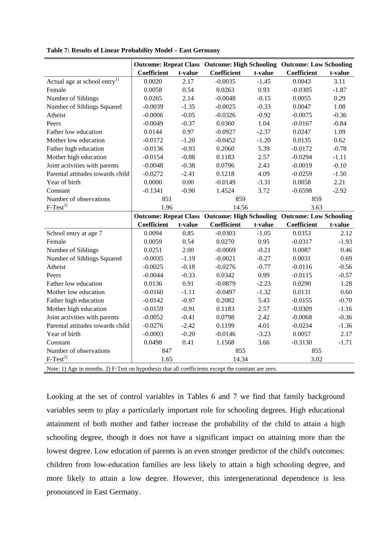
Table 7: Results of Linear Probability Model – East Germany
Outcome: Repeat Class Outcome: High Schooling Outcome: Low Schooling Coefficient t-value Coefficient t-value Coefficient t-value Actual age at school entry1) 0.0020 2.17 -0.0035 -1.45 0.0043 3.11 Female 0.0058 0.54 0.0263 0.93 -0.0305 -1.87 Number of Siblings 0.0265 2.14 -0.0048 -0.15 0.0055 0.29 Number of Siblings Squared -0.0039 -1.35 -0.0025 -0.33 0.0047 1.08 Atheist -0.0006 -0.05 -0.0326 -0.92 -0.0075 -0.36 Peers -0.0049 -0.37 0.0360 1.04 -0.0167 -0.84 Father low education 0.0144 0.97 -0.0927 -2.37 0.0247 1.09 Mother low education -0.0172 -1.20 -0.0452 -1.20 0.0135 0.62 Father high education -0.0136 -0.93 0.2060 5.39 -0.0172 -0.78 Mother high education -0.0154 -0.88 0.1183 2.57 -0.0294 -1.11 Joint activities with parents -0.0048 -0.38 0.0796 2.43 -0.0019 -0.10 Parental attitudes towards child -0.0272 -2.41 0.1218 4.09 -0.0259 -1.50 Year of birth 0.0000 0.00 -0.0149 -3.31 0.0058 2.21 Constant -0.1341 -0.90 1.4524 3.72 -0.6598 -2.92 Number of observations 851 859 859 F-Test2) 1.96 14.56 3.63 Outcome: Repeat Class Outcome: High Schooling Outcome: Low Schooling Coefficient t-value Coefficient t-value Coefficient t-value School entry at age 7 0.0094 0.85 -0.0303 -1.05 0.0353 2.12Female 0.0059 0.54 0.0270 0.95 -0.0317 -1.93Number of Siblings 0.0251 2.00 -0.0069 -0.21 0.0087 0.46Number of Siblings Squared -0.0035 -1.19 -0.0021 -0.27 0.0031 0.69Atheist -0.0025 -0.18 -0.0276 -0.77 -0.0116 -0.56Peers -0.0044 -0.33 0.0342 0.99 -0.0115 -0.57Father low education 0.0136 0.91 -0.0879 -2.23 0.0290 1.28Mother low education -0.0160 -1.11 -0.0497 -1.32 0.0131 0.60Father high education -0.0142 -0.97 0.2082 5.43 -0.0155 -0.70Mother high education -0.0159 -0.91 0.1183 2.57 -0.0309 -1.16Joint activities with parents -0.0052 -0.41 0.0798 2.42 -0.0068 -0.36Parental attitudes towards child -0.0276 -2.42 0.1199 4.01 -0.0234 -1.36Year of birth -0.0003 -0.20 -0.0146 -3.23 0.0057 2.17Constant 0.0498 0.41 1.1568 3.66 -0.3130 -1.71Number of observations 847 855 855 F-Test2) 1.65 14.34 3.02 Note: 1) Age in months. 2) F-Test on hypothesis that all coefficients except the constant are zero.
Looking at the set of control variables in Tables 6 and 7 we find that family background
variables seem to play a particularly important role for schooling degrees. High educational
attainment of both mother and father increase the probability of the child to attain a high
schooling degree, though it does not have a significant impact on attaining more than the
lowest degree. Low education of parents is an even stronger predictor of the child's outcomes:
children from low-education families are less likely to attain a high schooling degree, and
more likely to attain a low degree. However, this intergenerational dependence is less
pronounced in East Germany.

- 21 -
With respect to the probability of repeating a class parental education does not play
such an important role. Rather, there seem to be systematic gender differences and differences
between birth cohorts. Females and earlier birth cohort display a lower probability to repeat a
class. For all outcomes positive parental attitudes towards their child also exhibit a
qualitatively positive impact in both parts of Germany. Estimation results for the covariates
also do not seem to differ much between both models, i.e. it does not seem to make a
difference whether age at school entry is modeled as a continuous or categorical variable.
(ii) Matching on the propensity score
The second identification strategy – propensity score matching – aims at obtaining an
improved counterfactual by matching treated observations (i.e. individuals who entered
school at the age of seven) with truly comparable (in terms of observed covariates)
comparison observations (i.e. individuals who entered school at the age of six). Typically,
matching approaches aim at getting rid of unobserved heterogeneity by controlling for pre-
treatment outcomes. If there are unobserved differences between treatment and comparison
groups and these differences are persistent over time, then they should be reflected in the
value of the outcome prior to the intervention and, thus, controlling for pre-treatment
outcomes captures these unobservable differences. However, in the case at hand this is
obviously not possible and, hence, unobserved heterogeneity remains a potential problem. In
consequence, following the argument above, it cannot be ruled out that unconfoundedness
does not hold for our sample.
Tables 7 and 8 report treatment effect estimates for West and East Germany
considering the dummy treatment model and three caliper distances each. We observe that, as
the caliper narrows and precision – i.e. comparability – of the match increases, the number of
matches found is reduced. Roughly, we move from around 97% matches found for the widest
caliper to around 83% for the narrowest caliper in West Germany. In East Germany the share
of treated individuals finding a matching partner is somewhat lower (ranging from around
91% to 61%) due to the smaller pool of comparison units.

Table 8: Results of Propensity Score Matching – West Germany Caliper No. of Matches ATET Standard- t-value
(in % of treated) Error Outcome: Repeat Class
(i) 1/100*Standarddeviation 396 (96.6%) 0.047 0.023 2.10 (ii) 1/200*Standarddeviation 375 (91.5%) 0.044 0.024 1.83 (iii) 1/400*Standarddeviation 341 (83.2%) 0.039 0.026 1.51 Outcome: High Schooling (i) 1/100*Standarddeviation 397 (96.8%) –0.059 0.024 –2.43 (ii) 1/200*Standarddeviation 374 (91.2%) –0.053 0.026 –2.01 (iii) 1/400*Standarddeviation 340 (82.9%) –0.064 0.029 –2.21 Outcome: Low Schooling (i) 1/100*Standarddeviation 397 (96.8%) 0.041 0.025 1.61 (ii) 1/200*Standarddeviation 374 (91.2%) 0.034 0.028 1.23 (iii) 1/400*Standarddeviation 340 (82.9%) 0.030 0.030 1.00 Notes: Number of treated observations: 410; Number of observations in potential comparison pool: 1,308. Table 9: Results of Propensity Score Matching – East Germany Caliper No. of Matches ATET Standard- t-value
(in % of treated) Error Outcome: Repeat Class
(i) 1/100*Standarddeviation 293 (91.0%) 0.009 0.011 0.85 (ii) 1/200*Standarddeviation 245 (76.1%) 0.003 0.010 0.30 (iii) 1/400*Standarddeviation 193 (59.9%) –0.004 0.014 –0.28 Outcome: High Schooling (i) 1/100*Standarddeviation 295 (91.6%) –0.022 0.031 –0.69 (ii) 1/200*Standarddeviation 258 (80.1%) 0.012 0.034 0.35 (iii) 1/400*Standarddeviation 195 (60.6%) 0.015 0.039 0.40 Outcome: Low Schooling (i) 1/100*Standarddeviation 295 (91.6%) 0.030 0.018 1.62 (ii) 1/200*Standarddeviation 258 (80.1%) 0.022 0.019 1.14 (iii) 1/400*Standarddeviation 195 (60.6%) 0.013 0.023 0.58 Number of treated observations: 322; Number of observations in potential comparison pool: 525.
For West Germany matching results largely resemble the results found in the linear
probability models for both schooling degrees and the probability of class repetition. That is,
we still observe a qualitatively negative relationship between school entry age and educational
outcomes. For the Eastern part of the country, the comparison of truly comparable individuals
delivers no significant differences for all considered educational outcomes. However, the
question remains whether matching indeed identifies the correct effect.
(iii) Instrumental variable approach
In order to use exogenous variation to identify the causal effect of age at school entry on
schooling outcomes, we instrument age at school entry using the age at which an individual
should have entered school according to school entry regulations, as delineated in section 3.

- 23 -
Tables A.3 and A.4 in the Appendix report the first-stage IV results for West and East
Germany, respectively. The estimates show a strong positive correlation between the
instrument and age at school entry, for both models (continuous and binary instrument) and
for both parts of the country. That is, we observe a sufficiently high compliance with school
entry regulations in our sample.
Tables 10 and 11 report the instrumental variable estimates for West and East
Germany, respectively, where the upper panels show estimates for the model with the
continuous instrument. Regarding the set of control variables it is interesting to note that
estimation results are very similar – both in sign and magnitude – to those reported for the
linear probability models above. Specifically, background information on parental education
and attitudes retains its importance. The main result is unambiguous: The IV estimates find no
significant effect of age at school entry on any of the outcome measures, neither for the model
with the continuous regressor nor the dummy treatment model, neither for West nor East
Germany.
In our build-up of three different identification strategies we would argue that the IV
estimates are least likely to suffer from bias due to unobserved heterogeneity. Interpreting
these estimates, we find there is no indication of an effect of age at school entry on schooling
outcomes, i.e. no effect of simply being older at school enrolment on educational attainment
or the probability of repeating a class. The negative association between age at school entry
and schooling degree and the positive association between age at school entry and probability
of repeating a class found in LPM estimates and the matching approach seem to be selection
effects, i.e. driven by unobserved heterogeneity, perhaps systematic differences in ability.

Table 10: Instrumental Variable Estimates – West Germany
Outcome: Repeat Class Outcome: High Schooling Outcome: Low Schooling Coefficient t-value Coefficient t-value Coefficient t-value Actual age at school entry1) -0.0097 -0.91 -0.0002 -0.02 -0.0001 -0.01 Female -0.0546 -2.87 -0.0094 -0.46 -0.1027 -5.08 Number of Siblings 0.0225 1.14 0.0372 1.76 -0.0671 -3.21 Number of Siblings Squared -0.0029 -0.67 -0.0104 -2.25 0.0180 3.94 Atheist 0.1246 3.96 -0.0221 -0.65 -0.0462 -1.38 Peers 0.0074 0.29 -0.0357 -1.29 -0.0294 -1.08 Father low education 0.0369 1.38 -0.1711 -5.98 0.2237 7.89 Mother low education -0.0748 -2.92 -0.1008 -3.66 0.1148 4.21 Father high education 0.0125 0.40 0.1923 5.74 -0.0310 -0.93 Mother high education -0.0086 -0.24 0.1301 3.39 -0.0206 -0.54 Joint activities with parents -0.0055 -0.24 -0.0006 -0.02 -0.0465 -1.92 Parental attitudes towards child -0.0522 -2.69 0.0599 2.87 -0.0535 -2.59 Year of birth 0.0059 1.92 -0.0070 -2.15 -0.0028 -0.88 Constant 0.6061 0.66 0.9158 0.92 0.4848 0.49 Number of observations 1,786 1,788 1,788 F-Test2) 4.29 35.34 28.05 Outcome: Repeat Class Outcome: High Schooling Outcome: Low Schooling Coefficient t-value Coefficient t-value Coefficient t-value School entry at age 7 -0.0851 -0.75 -0.1013 -0.82 0.1634 1.32 Female -0.0566 -2.96 -0.0108 -0.52 -0.0985 -4.71 Number of Siblings 0.0170 0.87 0.0404 1.91 -0.0690 -3.22 Number of Siblings Squared -0.0015 -0.35 -0.0111 -2.40 0.0184 3.92 Atheist 0.1259 3.88 -0.0308 -0.88 -0.0450 -1.27 Peers 0.0026 0.10 -0.0426 -1.51 -0.0310 -1.08 Father low education 0.0399 1.51 -0.1754 -6.11 0.2314 7.97 Mother low education -0.0751 -2.92 -0.0968 -3.48 0.1142 4.05 Father high education 0.0057 0.18 0.1986 5.84 -0.0226 -0.66 Mother high education 0.0101 0.28 0.1161 2.96 -0.0260 -0.65 Joint activities with parents 0.0013 0.06 -0.0093 -0.38 -0.0392 -1.59 Parental attitudes towards child -0.0538 -2.74 0.0604 2.84 -0.0480 -2.23 Year of birth 0.0061 1.99 -0.0063 -1.90 -0.0021 -0.63 Constant -0.1530 -0.70 0.8757 3.71 0.3757 1.57 Number of observations 1,716 1,718 1,718 F-Test2) 4.06 33.86 26.10 Note: 1) Age in months. 2) F-Test on hypothesis that all coefficients except the constant are zero.

Table 11: Instrumental Variable Estimates – East Germany
Outcome: Repeat Class Outcome: High Schooling Outcome: Low Schooling Coefficient t-value Coefficient t-value Coefficient t-value Actual age at school entry1) 0.0030 1.43 0.0036 0.65 0.0031 0.97 Female 0.0060 0.56 0.0274 0.97 -0.0307 -1.88 Number of Siblings 0.0270 2.17 -0.0011 -0.03 0.0049 0.26 Number of Siblings Squared -0.0040 -1.39 -0.0034 -0.44 0.0049 1.11 Atheist 0.0004 0.03 -0.0256 -0.71 -0.0087 -0.42 Peers -0.0053 -0.40 0.0337 0.97 -0.0163 -0.82 Father low education 0.0146 0.98 -0.0915 -2.33 0.0245 1.08 Mother low education -0.0174 -1.22 -0.0469 -1.24 0.0138 0.63 Father high education -0.0134 -0.92 0.2073 5.39 -0.0175 -0.79 Mother high education -0.0147 -0.84 0.1241 2.67 -0.0304 -1.14 Joint activities with parents -0.0043 -0.34 0.0825 2.50 -0.0024 -0.12 Parental attitudes towards child -0.0271 -2.40 0.1219 4.08 -0.0259 -1.50 Year of birth 0.0002 0.11 -0.0134 -2.90 0.0055 2.07 Constant -0.2317 -0.98 0.7656 1.22 -0.5431 -1.51 Number of observations 851 859 859 F-Test2) 1.76 14.28 2.96 Outcome: Repeat Class Outcome: High Schooling Outcome: Low Schooling Coefficient t-value Coefficient t-value Coefficient t-value School entry at age 7 -0.0112 -0.57 0.0457 0.88 0.0004 0.01 Female 0.0049 0.45 0.0306 1.07 -0.0333 -2.03 Number of Siblings 0.0251 2.00 -0.0068 -0.21 0.0086 0.45 Number of Siblings Squared -0.0035 -1.21 -0.0019 -0.25 0.0030 0.67 Atheist -0.0031 -0.23 -0.0249 -0.70 -0.0128 -0.62 Peers -0.0040 -0.30 0.0332 0.96 -0.0110 -0.55 Father low education 0.0139 0.93 -0.0887 -2.25 0.0294 1.29 Mother low education -0.0166 -1.15 -0.0477 -1.26 0.0122 0.56 Father high education -0.0143 -0.97 0.2087 5.42 -0.0157 -0.71 Mother high education -0.0179 -1.02 0.1256 2.70 -0.0343 -1.28 Joint activities with parents -0.0056 -0.44 0.0811 2.45 -0.0074 -0.39 Parental attitudes towards child -0.0274 -2.40 0.1187 3.95 -0.0228 -1.32 Year of birth -0.0006 -0.32 -0.0137 -3.01 0.0053 2.00 Constant 0.0742 0.60 1.0645 3.30 -0.2706 -1.46 Number of observations 847 855 855 F-Test2) 1.61 14.19 2.66 Note: 1) Age in months. 2) F-Test on hypothesis that all coefficients except the constant are zero.
- 26 -
5. Conclusions The question at which age a child should ideally enter school remains a controversial topic in
German education policy: Is the established regulation still appropriate? Should deferment be
encouraged? Or should the focus be on school enrolment at younger ages? Answering these
questions is also of broader interest, since many countries have similar compulsory schooling
laws, and an emerging literature in empirical educational economics focuses on studying these
regulations.
This paper has aimed at contributing novel empirical evidence regarding the effect of
age at school entry on educational attainment. We have discussed school enrolment
regulations in West and East Germany, and delineated the policy relevance of the question
whether age at school entry has any effect on educational outcomes. To assess this question,
we have developed an empirical strategy based on a longitudinal survey of young adults in
Germany in the early to mid-1990s. The data focus on the respondents' transition from
childhood to adolescence and then on to adulthood during the 1960s through the 1980s,
containing, in particular, core information on the child and her parents, and the parent-child
relationship. The latter control variable is of especial importance, as it captures information
likely playing a role in enrolment decisions. Individuals in our sample entered school at some
point in time during the period 1966 to 1980, a period during which enrolment regulations
were clearly defined and did not change, but did allow for exceptions such as early enrolment
and deferment, especially in West Germany.
The two outcomes we consider, probability of repeating a class and eventual schooling
degree attained, assess short-term as well as long-term schooling success. As treatment
variables we use (a) the age at school entry in months as a continuous regressor, and (b) a
binary regressor capturing whether the individual entered at age 7 or at age 6. We have
assessed treatment effects using three identification strategies. Linear probability models
suggest a qualitatively negative association between deferment and schooling performance,
for both West and East Germany. This result, with some refinement, is borne out by
propensity score matching estimates. We think that these findings are likely driven by
unobserved heterogeneity, i.e. those individuals who entered late did do so since they were
conjectured (by their parents or elementary school teachers) to display low educational
performance. We have then argued that our third identification strategy, instrumenting the
actual age at enrolment with the age at enrolment according to the regulation, is most likely to
control for unobserved ability differences and thus to reveal the "true" effect of age at school
entry on educational outcomes. The findings suggest that there is no such effect, neither on

- 27 -
schooling degrees nor on the probability of repeating a class, neither for West nor for East
Germany.
We conclude that holding children back one year does not seem to secure a better
schooling performance for this group, i.e. we find no justification for the rationale behind
deferring children. If anything, then some of the deferred seem to fare worse, but this appears
to be due to negative selection into this group. What policy recommendations could be
derived from this result? First, there seems to be no reason to defer a child unless there are
indications that she will not be able to follow class, i.e. no child should be deferred who
seems perfectly capable of following class at age 6 – this basically invalidates the cut-off date
rule. Second, this points to the importance of individual schooling tests, to refine the selection
process.
One important issue in this discussion is the question whether children should enroll at
even younger ages. Unfortunately, we cannot say much about this, as only few individuals in
our data entered school at age 5. It is clearly an interesting research question worth being
investigated empirically, but additional data would be needed. Still, we have found that for a
particular child it does not seem to matter in terms of schooling outcomes whether the child
enrolls at age 6 or age 7.
Potentially, this finding has wider implications. Consider the case of Germany, where
– in a simplified argument – the regular retirement age is 65. If the same particular child
indeed attains the same schooling outcome under enrolment at age 6 or at age 7, she leaves
school with the same level of human capital either in a given year or one year later. If her
retirement age is a given constant, then her productivity is available to the labor market one
year more or less, and she would be paying taxes and be contributing to public pension funds
and social security one year more or less. Moreover, if, for instance, German mothers were to
return to work only after their child has enrolled in school, it would matter for the length of
their productive contribution to the labor market as well if the child enters at age 6 or at age 7.
References ANGRIST, J. D. and A. B. KRUEGER (1992), The Effect of Age at School Entry on Educational Attainment: An Application of Instrumental Variables with Moments from Two Samples. Journal of the American Statistical Association 87, 328-336. BARTH, K. (1997), Ist die Schuleingangsdiagnostik überflüssig?, Grundschule 7-8, 63-65.

- 28 -
COMENIUS (1633 in German, originally 1628/1631), Informatorium der Mutterschul, as cited in Rüdiger et al. (1976) p.14. CURRIE, J. (2001), Early Childhood Education Programs, Journal of Economic Perspectives 15, 213-238. DEHEJIA, R.H. and S. WAHBA (2002), Propensity Score-Matching Methods for Nonexperimental Causal Studies, Review of Economics and Statistics 84, 151-161. DEL BONO, E. and F. GALINDO-RUEDA (2004), "Do a Few Months of Compulsory Schooling Matter? The Education and Labour Market Impact of School Leaving Rules", IZA Discussion Paper 1233, Bonn. FREDRIKSSON, P. and B. ÖCKERT (2004), "Is Early Learning Really More Productive? The Effect of School Starting Age on School and Labor Market Performance", mimeo, Dept. of Economics, Uppsala University, November 2004. HECKMAN, J.J. (2000), "Policies to Foster Human Capital", Research in Economics 54, 3-56. HOLLAND, P.W. (1986), Statistics and Causal Inference (with discussion), Journal of the American Statistical Association 81, 945-970. IMBENS, G.W. (2000), The role of the propensity score in estimating dose-response functions, Biometrika 87, 706-710. KLUVE, J. (2003), Assessing Counterfactuals when Treatment is Multivalued, revised version of UC Berkeley Center for Labor Economics Working Paper #55. LEUVEN, E., M. LINDAHL, H. OOSTERBEEK and D. WEBBINK (2004), "New evidence on the effect of time in school on early achievement", mimeo, University of Amsterdam. MEIERS, K. (2002), Problem Schulfähigkeit, Grundschule 5, 10-12. ROSENBAUM, P. R. (1995), Observational Studies, Springer: New York et al. ROSENBAUM, P. R. and D. B. RUBIN (1983), The central role of the propensity score in observational studies for causal effects, Biometrika 70, 41-55. RÜDIGER, D., A. KORMANN and H. PEEZ (1976), Schuleintritt und Schulfähigkeit – Zur Theorie und Praxis der Einschulung, Ernst Reinhardt Verlag: München, Basel. SCHAVAN, A. and P. WENDT (2000), "Sollen Kinder ab 5 Jahren in die Schule gehen?", Grundschule 5, 48-50. STRØM, B. (2003), "Student Achievement and Birthday Effects", mimeo, Dept. of Economics, Norwegian University of Science and Technology Trondheim. WENDT, P. (2003), Streitfall "Einschulungsalter", www.praxisgrundschule.de/forum/einschulungsalter.pdf

- 29 -
Appendix Table A.1: Description of Variables Variable Description Outcome Measures Highest Schooling Degree Categorical variable capturing 3 schooling degrees: (A) no schooling degree or completed secondary (Hauptschule); (B) intermediary degree (Realschule), (C) upper secondary or technical schooling degree (Abitur). In the analysis, the indicator variable "low schooling degree"=1 if (A) is the case, 0 otherwise; and indicator variable "high schooling degree"=1 if (C) is the case, 0 otherwise. Repeat Class Indicator variable taking on the value 1 if respondent reported having repeated a school year at some stage during her education; 0 otherwise. Treatment Variables Actual age at school entry Age at school entry in month. School entry at age 7 Indicator variable taking on the value 1 if respondent entered school at the age of Seven; 0 if individual entered at the age of six (all other observations were dropped). Control Variables Female Indicator variable taking on the value 1 if respondent is female; 0 otherwise. Year of birth Year of birth of the respondent. Number of Siblings Number of siblings of respondent. Atheist Indicator variable taking on the value 1 if respondent reported no religious denomination; 0 otherwise Peers Indicator variable taking on the value 1 if respondent reported having had friends during childhood and adolescence; 0 otherwise. Father low education Indicator variable taking on the value 1 if respondent's father has no schooling degree or completed secondary schooling degree; 0 otherwise. Mother low education Indicator variable taking on the value 1 if respondent's mother has no schooling degree or completed secondary schooling degree; 0 otherwise. Father high education Indicator variable taking on the value 1 if respondent's father has upper secondary or technical schooling degree; 0 otherwise. Mother high education Indicator variable taking on the value 1 if respondent's mother has upper secondary or technical schooling degree; 0 otherwise. Joint activities Indicator variable taking on the value 1 if respondent reported having shared at least two of the following four joint activities with her parents during childhood: reading, sports, music and sharing other hobbies; 0 otherwise. Parental attitudes Indicator variable taking on the value 1 if respondent reported her parents having had at least two of the following four positive attitudes towards her during childhood: to put hope into the child, to believe that the child is highly able, to be ambitious with the child and to have plans with the child; 0 otherwise. Instrumental Variables Age at school entry according (i) Age in months at which an individual should have entered school if school entry to regulation regulations had been complied with perfectly. (ii) Dummy variable taking on the value of 1 if an individual is born in June/July (West Germany) or June/July/August (East Germany).

- 30 -
Table A.2: Summary Statistics – West and East Germany West Germany East Germany Mean Std.dev. Mean Std.dev. Outcome measures Repeat class 0.19 0.39 0.03 0.16 High schooling 0.35 0.48 0.28 0.45 Low schooling 0.30 0.46 0.06 0.24 Treatment variables Actual age at school entry 79.52 6.42 81.94 5.86 School entry at age 7 a) 0.24 0.43 0.38 0.49 Control variables Female 0.50 0.50 0.48 0.50 Number of Siblings 1.36 1.17 1.32 1.04 Number of Siblings Squared 3.22 5.34 2.81 4.46 Atheist 0.11 0.31 0.80 0.40 Peers 0.84 0.37 0.79 0.41 Father low education 0.55 0.50 0.34 0.47 Mother low education 0.61 0.49 0.39 0.49 Father high education 0.23 0.42 0.25 0.44 Mother high education 0.12 0.32 0.14 0.35 Joint activities with parents 0.27 0.45 0.27 0.45 Parental attitudes towards child 0.60 0.49 0.64 0.48 Year of birth 67.6 3.24 67.9 3.16 Instrumental variables School entry age in months acc. to regulation 79.39 3.53 80.36 3.57 School entry at age 7 acc. to regulation a) 0.18 0.39 0.25 0.44 Number of observations 1788 859 Note: a) Individuals who entered school at age 5 or age 8 excluded.

Table A.3: First-Stage IV Estimates – West Germany Sample: Repeat Class Sample: Schooling Degree Coefficient t-value Coefficient t-value Female 0.1354 0.44 0.1457 0.48 Number of Siblings -0.2605 -0.83 -0.2627 -0.84 Number of Siblings Squared 0.0376 0.54 0.0380 0.55 Atheist -0.0461 -0.09 -0.0835 -0.17 Peers -0.2029 -0.49 -0.2135 -0.52 Father low education -0.2582 -0.61 -0.2627 -0.62 Mother low education 0.1582 0.38 0.1512 0.37 Father high education -0.1923 -0.39 -0.1976 -0.40 Mother high education -0.3503 -0.61 -0.3849 -0.68 Joint activities with parents -0.5375 -1.54 -0.5377 -1.55 Parental attitudes towards child -0.0026 -0.01 -0.0013 0.00 Year of birth -0.0350 -0.73 -0.0367 -0.77 Age according to regulation1) 0.2541 5.86 0.2532 5.85 Constant 62.3444 12.30 62.5379 12.36 Number of observations 1,786 1,788 F-Test2) 3.38 3.39 Model with Dummy for School Entry at Age 7 Female 0.0132 0.64 0.0137 0.67 Number of Siblings 0.0000 0.00 -0.0002 -0.01 Number of Siblings Squared 0.0005 0.10 0.0005 0.11 Atheist 0.0440 1.28 0.0417 1.22 Peers 0.0288 1.04 0.0282 1.02 Father low education -0.0017 -0.06 -0.0019 -0.07 Mother low education -0.0052 -0.19 -0.0055 -0.20 Father high education -0.0061 -0.18 -0.0065 -0.19 Mother high education 0.0095 0.25 0.0075 0.19 Joint activities with parents -0.0374 -1.60 -0.0373 -1.60 Parental attitudes towards child -0.0241 -1.15 -0.0241 -1.15 Year of birth -0.0044 -1.38 -0.0045 -1.41 Entry at age 7 according to regulation 0.2170 8.27 0.2157 8.23 Constant 0.4894 2.21 0.4967 2.25 Number of observations 1,716 1,718 F-Test2) 6.29 6.24 Note: 1) Age in months. 2) F-Test on hypothesis that all coefficients except the constant are zero.

Table A.4: First-Stage IV Estimates – East Germany Sample: Repeat Class Sample: Schooling Degree Coefficient t-value Coefficient t-value Female -0.2034 -0.56 -0.1560 -0.43 Number of Siblings -0.7662 -1.81 -0.8097 -1.93 Number of Siblings Squared 0.1835 1.88 0.1950 2.00 Atheist -1.1037 -2.41 -1.1165 -2.45 Peers 0.0945 0.21 0.0043 0.01 Father low education -0.0369 -0.07 -0.0714 -0.14 Mother low education 0.2192 0.45 0.2297 0.48 Father high education -0.4337 -0.88 -0.4175 -0.85 Mother high education -0.8960 -1.51 -0.9552 -1.61 Joint activities with parents -0.4122 -0.97 -0.3394 -0.81 Parental attitudes towards child -0.2432 -0.63 -0.1996 -0.52 Year of birth -0.0760 -1.29 -0.0763 -1.31 Age according to regulation1) 0.7194 14.02 0.7170 13.98 Constant 31.0922 5.02 31.3870 5.08 Number of observations 851 859 F-Test2) 17.18 17.04 Model with Dummy for School Entry at Age 7 Female -0.0284 -1.01 -0.0255 -0.91 Number of Siblings -0.0331 -1.02 -0.0368 -1.13 Number of Siblings Squared 0.0059 0.77 0.0068 0.90 Atheist -0.0615 -1.74 -0.0640 -1.81 Peers 0.0115 0.33 0.0034 0.10 Father low education 0.0154 0.40 0.0113 0.29 Mother low education -0.0081 -0.22 -0.0057 -0.15 Father high education -0.0215 -0.56 -0.0229 -0.60 Mother high education -0.0875 -1.92 -0.0902 -1.98 Joint activities with parents -0.0418 -1.28 -0.0367 -1.13 Parental attitudes towards child -0.0038 -0.13 0.0008 0.03 Year of birth -0.0039 -0.86 -0.0040 -0.90 Entry at age 7 according to regulation 0.6251 19.51 0.6236 19.47 Constant 0.5942 1.89 0.6117 1.96 Number of observations 847 855 F-Test2) 30.64 30.51 Note: 1) Age in months. 2) F-Test on hypothesis that all coefficients except the constant are zero.