The Effects of Physician Prescribing Behaviors on

Prescription Drug Use and Labor Supply: Evidence from

Movers in Denmark

⇤

Jessica Laird and Torben Nielsen

March 16, 2017

Abstract

Health is an increasingly critical determinant of labor supply as the population ages and asa growing fraction of labor force participants develop chronic conditions. Prescription drugs tocontrol pain and mental health disorders have the potential to raise labor supply, but abuse of andaddiction to some drugs (such as opioids) could work in the opposite direction. Thus, physicianprescribing tendencies could impact patients’ ability to work. In this paper, we estimate theimpacts of physicians with differential prescribing behaviors on patient prescription drug use andlabor market outcomes for the four classes of prescription drugs used most frequently to treatmusculoskeletal and mental health disorders: opioids, anti-inflammatories, anti-anxiety drugs,and anti-depressants. We use Danish administrative data on the full population of the 1925 to1980 birth cohorts and link information on individual’s prescription drug use, their primary carephysicians, municipality of residence, and labor market outcomes from 1995 to 2013. We exploitquasi-random separations of individuals from their physicians associated with geographic movesacross municipalities to estimate the causal impact of physician prescribing rates on individualprescription drug use and labor market outcomes. We find that having a general practitionerwho has a 10 percentage point higher opioid prescription rate leads to a 4.5 percentage pointincrease in the probability an individual uses prescribed opioids, as well as a (significant) 1.2percentile decrease in their labor income rank and a 1.5 percentage point decrease in their laborforce participation. Changes in physician prescribing rates lead to similar changes in prescriptiondrug use for the other classes of prescription drugs, but they are not associated with any discernibleeffect on labor market outcomes.

⇤We thank Amitabh Chandra, Raj Chetty, David Cutler, Itzik Fadlon, James Feigenbaum, John Friedman, ClaudiaGoldin, Nathan Hendren, Lawrence Katz, and numerous seminar participants for helpful comments and discussions.This research was supported by the National Institute on Aging of the National Institutes of Health under grant numberT32-AG000186 and by the Danish Council for Independent Research under grant number 11-104234. The content isthe sole responsibility of the authors and does not necessarily represent the official views of the National Institutes ofHealth.

1 Introduction

Much evidence indicates that health is a critical determinant of labor supply (e.g. Currie and Madrian

1999, Cai and Cong 2009, Gaskin and Richard 2012, Cai, Mavromavas, and Oguzoglu 2013, Dobkin

et al. 2016, Fadlon and Nielsen 2016). In the United States, over one half of the prime age males not

in the labor force have a debilitating condition (Krueger 2016). Gaskin and Richard (2012) estimate

that the loss in productivity due just to pain is approximately $300 billion a year. Furthermore, this

is increasingly a problem: from 1999 to 2013, mid-life morbidity (including self-reported declines in

mental health, and increases in chronic pain and inability to work) among white Non-Hispanics in the

United States increased after decades of improvement (Case and Deaton 2015).

Applications to disability insurance suggest that musculoskeletal and mental health disorders are

the most prominent conditions that keep individuals from working (Maestas, Mullen, and Strand 2013).

Such conditions are often treated with prescription medications. For example, one half of U.S. men

whose health prevents them from working take pain medication on a daily basis (Krueger 2016). There

is, however, substantial variation in how physicians treat musculoskeletal and mental health conditions,

and it remains unclear how variation in treatment affects labor supply.

In this paper, we use variation in physicians’ prescribing rates of medications used to treat debili-

tating conditions to estimate the impacts of physician prescribing behaviors on patient labor supply.1

In particular, we study how quasi-experimental changes in the physician prescribing rates experienced

by an individual associated with a geographic move affects that patient’s prescription drug use and

labor market outcomes.

Although the medical literature shows that the use of approved prescription drugs can improve

health in the short run, much less is known about whether such prescription drug use can translate

into sustained improvements in labor market outcomes. Even the direction of impacts of prescription

drug use on labor market outcomes is potentially ambiguous. For example, opioids may effectively treat

pain and allow individuals with chronic pain to work, but they also are highly addictive and opioid

abuse may negatively influence long-term labor productivity and health.2 Opioids offer a particularly

stark contrast between short run relief and long run consequences, but other prescription drugs may

generate similar trade-offs.3 The effect that physician prescribing rates of drugs have on labor supply1This is a policy relevant question, given that most policies to change individual’s prescription drug use would likely

work through altering physician’s prescribing behaviors.2Opioid abuse is a substantial global problem: 15 million people worldwide suffer from opioid dependence (WHO).3Benzodiazepines are used to treat short-term anxiety and insomnia, however, they can lead to physical dependences

and adverse psychological and physical effects, as well as lead to overdoses (Ashton 2005).

1

remains a difficult question to answer due both to the sparsity of data that connects physicians,

prescription drug use, and labor market outcomes, and the potential endogeneity of physician choice.

To estimate the effects of physician prescribing rates, we use Danish administrative data, with which

we can link an individual’s labor supply, prescription drug use, general practitioner, and residence for

almost two decades. Our identification strategy exploits a quasi-random separation of an individual

from their general practitioner due to the patient moving to a new municipality. Because the choice

of the new physician may be endogenous to the patient’s health, we use the pre-move physician’s

prescribing rate to instrument for the change in physician prescribing rates. Since individuals with

prior doctors with different prescribing rates may have different trends in their health (for example

due to the effects of their doctor), we match individuals who move to similar individuals with similar

pre-period physician prescribing rates who do not move and assign them a placebo moving year. We

then take the triple difference in outcomes between the movers and non-movers, the individuals with

a high predicted change in physician prescribing rates and with a low predicted change, and after

the move minus before, to identify how different changes in prescribing rates affect individual’s own

prescription drug usage and their labor supply.

The main assumption for this strategy is that other determinants of the relative change in pre-

scription drug use and labor force participation between movers and non-movers are unrelated to the

pre-move physician’s prescribing rate, outside of its effects on the change in physician prescribing rates.

We discuss and address the main threats to this assumption later in the paper and find that they do not

bias our results. Our analysis focuses on 730,000 individuals in Denmark aged 30-70 who move across

municipalities from 1995-2013, as well as a matched sample of 1,530,000 individuals who do not move.

We evaluate the effects of physician prescribing rates for the four drugs that are the most widely used

to treat musculoskeletal and mental health disorders: opioids, anti-inflammatories, anti-depressants,

and anxiolytics.

Our analysis provides two sets of core results. The first set of results estimates how physicians

affect patient’s prescription drug use. We find that moving to a doctor that prescribes 1 percentage

point (pp) more opioids leads to an increase in opioid usage of .45 pp, with a standard error of .04

pp. Equivalently, moving to a doctor with a one standard deviation higher prescribing rate of opioids

leads to a .8 pp (12%) increase in individual’s opioid prescription drug use. We find similar sized

effects of the prescribing rates of other prescription drugs. This suggests that the choice of physician

has substantial effects on the treatment that individuals receive. The second set of results estimates

2

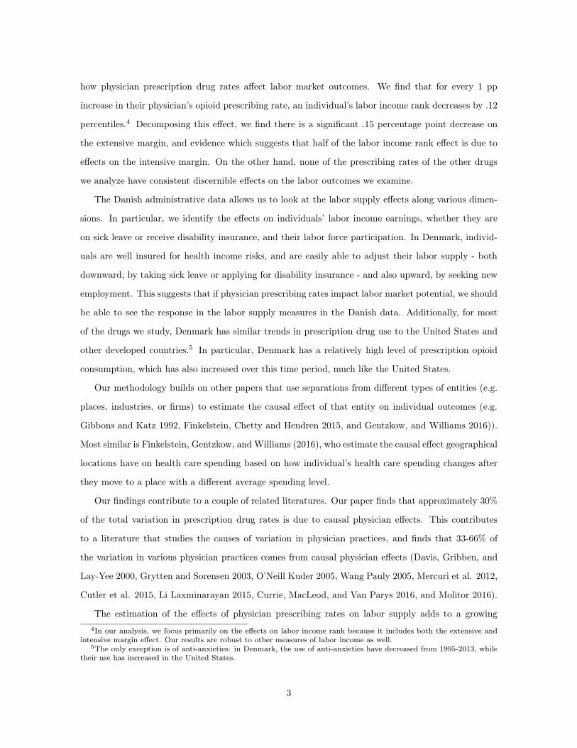
how physician prescription drug rates affect labor market outcomes. We find that for every 1 pp

increase in their physician’s opioid prescribing rate, an individual’s labor income rank decreases by .12

percentiles.4 Decomposing this effect, we find there is a significant .15 percentage point decrease on

the extensive margin, and evidence which suggests that half of the labor income rank effect is due to

effects on the intensive margin. On the other hand, none of the prescribing rates of the other drugs

we analyze have consistent discernible effects on the labor outcomes we examine.

The Danish administrative data allows us to look at the labor supply effects along various dimen-

sions. In particular, we identify the effects on individuals’ labor income earnings, whether they are

on sick leave or receive disability insurance, and their labor force participation. In Denmark, individ-

uals are well insured for health income risks, and are easily able to adjust their labor supply - both

downward, by taking sick leave or applying for disability insurance - and also upward, by seeking new

employment. This suggests that if physician prescribing rates impact labor market potential, we should

be able to see the response in the labor supply measures in the Danish data. Additionally, for most

of the drugs we study, Denmark has similar trends in prescription drug use to the United States and

other developed countries.5 In particular, Denmark has a relatively high level of prescription opioid

consumption, which has also increased over this time period, much like the United States.

Our methodology builds on other papers that use separations from different types of entities (e.g.

places, industries, or firms) to estimate the causal effect of that entity on individual outcomes (e.g.

Gibbons and Katz 1992, Finkelstein, Chetty and Hendren 2015, and Gentzkow, and Williams 2016)).

Most similar is Finkelstein, Gentzkow, and Williams (2016), who estimate the causal effect geographical

locations have on health care spending based on how individual’s health care spending changes after

they move to a place with a different average spending level.

Our findings contribute to a couple of related literatures. Our paper finds that approximately 30%

of the total variation in prescription drug rates is due to causal physician effects. This contributes

to a literature that studies the causes of variation in physician practices, and finds that 33-66% of

the variation in various physician practices comes from causal physician effects (Davis, Gribben, and

Lay-Yee 2000, Grytten and Sorensen 2003, O’Neill Kuder 2005, Wang Pauly 2005, Mercuri et al. 2012,

Cutler et al. 2015, Li Laxminarayan 2015, Currie, MacLeod, and Van Parys 2016, and Molitor 2016).

The estimation of the effects of physician prescribing rates on labor supply adds to a growing4In our analysis, we focus primarily on the effects on labor income rank because it includes both the extensive and

intensive margin effect. Our results are robust to other measures of labor income as well.5The only exception is of anti-anxieties: in Denmark, the use of anti-anxieties have decreased from 1995-2013, while

their use has increased in the United States.

3

literature that estimates the effect of prescription drugs on individual outcomes. An extensive medical

literature reviews the effects of medical drugs on health metrics, but often only over short periods of

time.6 Additionally, recent work estimates the effects of different prescription drugs on labor supply.

Kilby (2015) finds that a decrease in use of opioids due to the onset of the Prescription Monitoring

Program laws increases the number of absent days at work for individuals with workers’ compensation

injuries and those on short term disability with pain related diagnosis codes.7 Both Bütikofer and Skira

(2013) and Garthwaite (2012) look at the effect of Cox-2 inhibitors (part of the anti-inflammatory class)

on employment by looking at the abrupt removal of Vioxx from the market in 2004 and find a small

decrease in labor force participation due to the removal of Vioxx.8

The paper proceeds as follows: Section 2 details the data we use and the institutional framework

in Denmark. Section 3 outlines our empirical strategy. Section 4 estimates the effect of a change in

physician’s prescribing rate on individual’s drug use while Section 5 looks at the effect on labor market

outcomes. Section 6 concludes.

2 Data and Institutional Framework

2.1 Data Sources

The ideal data for an analysis of the impact of physician’s prescribing rate on labor supply contains

information on individual’s physicians, their prescription drug use, and their labor supply. We create

this dataset using several Danish administrative data sources to build a panel of individuals from

cohorts 1925-1980 covering the years 1995-2015, with information on their prescription drug use,

their general practitioner, multiple measures of labor supply, and their geographical history, which is6In medical control trials, opioids are found to decrease pain in the short term, but there is also a large amount of

drop out due to adverse events or lack of efficacy (Shaheed et al. 2016). In terms of long-term opioid therapy, in a reviewChou et al. (2015) find that “reliable conclusions about the effectiveness of long-term opioid therapy for chronic pain arenot possible due to the paucity of research to date.” Anti-inflammatories do decrease short term pain better than theplacebo, but have little benefit after two weeks of use, and serious adverse effects associated with them (Van Tudler etal. 2000, Bjordal et al. 2004, Lin et al. 2004). In a review, Dell’osso and Lader (2013) find that the risk benefit ratio forbenzodiazepines is positive in short-term use, but it remains unclear whether short-term benefits outweigh the possiblerisk of dependence. A large amount of evidence finds that anti-depressants are better than placebo on quality of life andpyschosocial outcomes, (Stewart et al. 1988, Ceulemans et al. 1985, Stewart et al. 1993, Kocsis et al. 1997, Lydiardet al. 1997, and Bollini 1999). The one medical control trial that we know of that looks at the effects of prescriptiondrugs on labor supply is a study by Agosti, Stewart, and Quitkin (1991) which randomly assigned an anti-depressant ora placebo and looked at labor outcomes (N=43). It found a negative effect on hours worked in the 6 weeks of follow-up,but it was not statistically significant.

7In the Section 6, we discuss the reasons why our two papers may have found different results.8There are a couple of additional papers that look at the effects of prescription drug types that we do not analyze in

this paper. Daysal and Orsini (2014) analyze the effect of Hormonal Replacement Therapy on employment of middle-agewomen using the timing of the release of information of the potential hazardous effects of HRT in 2002 and deduce thatHRT increases employment. Thirumurthy, Zivin, and Goldstein (2008) look at the effects of anti-virals on labor supplyin Africa. Finally, Currie, Stabile, and Jones (2014), look at the effects of ADHD use on education outcomes in Canada.

4

necessary for our particular identification strategy. In our analysis, we restrict our sample to individuals

aged 30-70 to cover the working age population.

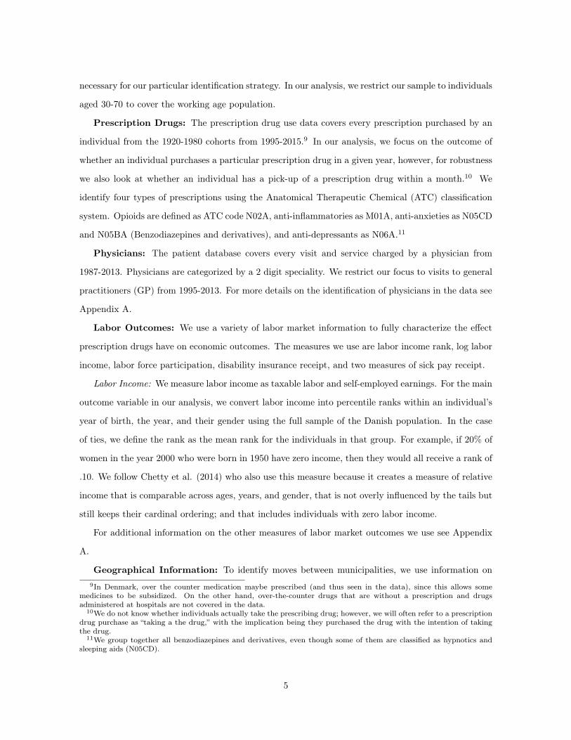
Prescription Drugs: The prescription drug use data covers every prescription purchased by an

individual from the 1920-1980 cohorts from 1995-2015.9 In our analysis, we focus on the outcome of

whether an individual purchases a particular prescription drug in a given year, however, for robustness

we also look at whether an individual has a pick-up of a prescription drug within a month.10 We

identify four types of prescriptions using the Anatomical Therapeutic Chemical (ATC) classification

system. Opioids are defined as ATC code N02A, anti-inflammatories as M01A, anti-anxieties as N05CD

and N05BA (Benzodiazepines and derivatives), and anti-depressants as N06A.11

Physicians: The patient database covers every visit and service charged by a physician from

1987-2013. Physicians are categorized by a 2 digit speciality. We restrict our focus to visits to general

practitioners (GP) from 1995-2013. For more details on the identification of physicians in the data see

Appendix A.

Labor Outcomes: We use a variety of labor market information to fully characterize the effect

prescription drugs have on economic outcomes. The measures we use are labor income rank, log labor

income, labor force participation, disability insurance receipt, and two measures of sick pay receipt.

Labor Income: We measure labor income as taxable labor and self-employed earnings. For the main

outcome variable in our analysis, we convert labor income into percentile ranks within an individual’s

year of birth, the year, and their gender using the full sample of the Danish population. In the case

of ties, we define the rank as the mean rank for the individuals in that group. For example, if 20% of

women in the year 2000 who were born in 1950 have zero income, then they would all receive a rank of

.10. We follow Chetty et al. (2014) who also use this measure because it creates a measure of relative

income that is comparable across ages, years, and gender, that is not overly influenced by the tails but

still keeps their cardinal ordering; and that includes individuals with zero labor income.

For additional information on the other measures of labor market outcomes we use see Appendix

A.

Geographical Information: To identify moves between municipalities, we use information on9In Denmark, over the counter medication maybe prescribed (and thus seen in the data), since this allows some

medicines to be subsidized. On the other hand, over-the-counter drugs that are without a prescription and drugsadministered at hospitals are not covered in the data.

10We do not know whether individuals actually take the prescribing drug; however, we will often refer to a prescriptiondrug purchase as “taking a the drug,” with the implication being they purchased the drug with the intention of takingthe drug.

11We group together all benzodiazepines and derivatives, even though some of them are classified as hypnotics andsleeping aids (N05CD).

5

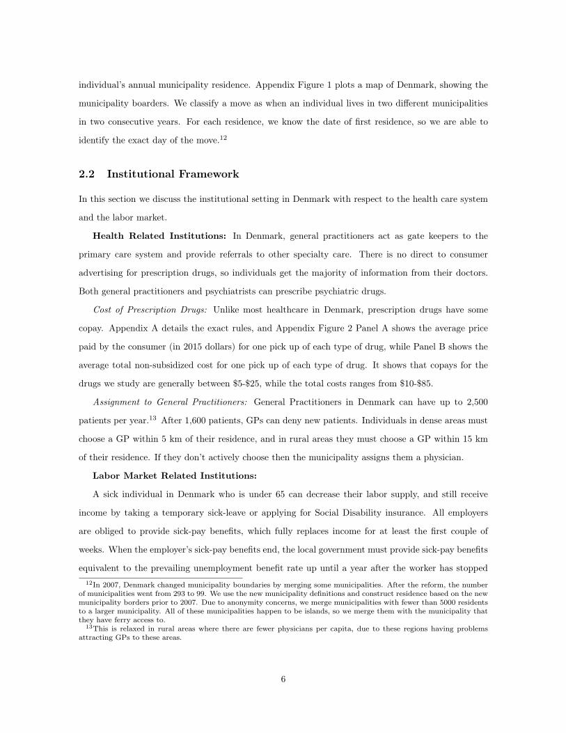
individual’s annual municipality residence. Appendix Figure 1 plots a map of Denmark, showing the

municipality boarders. We classify a move as when an individual lives in two different municipalities

in two consecutive years. For each residence, we know the date of first residence, so we are able to

identify the exact day of the move.12

2.2 Institutional Framework

In this section we discuss the institutional setting in Denmark with respect to the health care system

and the labor market.

Health Related Institutions: In Denmark, general practitioners act as gate keepers to the

primary care system and provide referrals to other specialty care. There is no direct to consumer

advertising for prescription drugs, so individuals get the majority of information from their doctors.

Both general practitioners and psychiatrists can prescribe psychiatric drugs.

Cost of Prescription Drugs: Unlike most healthcare in Denmark, prescription drugs have some

copay. Appendix A details the exact rules, and Appendix Figure 2 Panel A shows the average price

paid by the consumer (in 2015 dollars) for one pick up of each type of drug, while Panel B shows the

average total non-subsidized cost for one pick up of each type of drug. It shows that copays for the

drugs we study are generally between $5-$25, while the total costs ranges from $10-$85.

Assignment to General Practitioners: General Practitioners in Denmark can have up to 2,500

patients per year.13 After 1,600 patients, GPs can deny new patients. Individuals in dense areas must

choose a GP within 5 km of their residence, and in rural areas they must choose a GP within 15 km

of their residence. If they don’t actively choose then the municipality assigns them a physician.

Labor Market Related Institutions:

A sick individual in Denmark who is under 65 can decrease their labor supply, and still receive

income by taking a temporary sick-leave or applying for Social Disability insurance. All employers

are obliged to provide sick-pay benefits, which fully replaces income for at least the first couple of

weeks. When the employer’s sick-pay benefits end, the local government must provide sick-pay benefits

equivalent to the prevailing unemployment benefit rate up until a year after the worker has stopped12In 2007, Denmark changed municipality boundaries by merging some municipalities. After the reform, the number

of municipalities went from 293 to 99. We use the new municipality definitions and construct residence based on the newmunicipality borders prior to 2007. Due to anonymity concerns, we merge municipalities with fewer than 5000 residentsto a larger municipality. All of these municipalities happen to be islands, so we merge them with the municipality thatthey have ferry access to.

13This is relaxed in rural areas where there are fewer physicians per capita, due to these regions having problemsattracting GPs to these areas.

6

working. If the worker remains sick and unable to work, he or she can apply at the municipality level

for Social Disability Insurance (Social DI) benefits that provide income permanently. The program

is moderately generous - for example, in 2000, subject to income-testing against overall household

income, a successful application amounted to roughly DKK 127,500 ($16,000) per year.14

After turning 60, and before they reach the old-age pension retirement age, individuals who have

been members of a voluntary unemployment fund for a sufficiently long period are eligible for the Vol-

untary Early Retirement Pension (VERP). Approximately 80% of the population is eligible for VERP,

which provides an annual income that is 90% of previous earnings, but maxes at the unemployment

benefit level which was 148200 Kroner in 2000 ($18,525). At the full-retirement age of 67 (or 65 for

those born after July 1, 1939), all residents become eligible for the Old-Age Pension (OAP), which

provides income-tested annuities of up to roughly DKK 87,000 ($10,900) per year (at 2000 rates).15

2.3 Summary Statistics

2.3.1 Prescription Drug Summary Statistics

In Appendix Table 1, we present summary statistics for the sample we using in our analysis.16 For

prescription drug use, approximately 6.5% of the sample have an opioid prescription purchase within a

year. Alternatively, 19% purchase prescription anti-inflammatories, and 6-7% purchase anti-anxieties,

and 7-9% purchase anti-depressants.

Over the time period we study, prescription opioid use and anti-depressant use increased, while

anti-anxiety use decreased. Figure 1 shows the fraction of individuals who use the prescription drugs

we study by year from 1995-2015. Panel A shows that opioid prescription drug use has increased

steadily from 1995 (5%) to 2015 (9%). Panel B shows that anti-inflammatory use prevalence increased

from 16% use in 1995 to 22% use in 2005, at which point usage peaked, and started to decrease slightly.

Anti-anxiety use in Panel C has had a remarkable decrease in usage from 11% to 4% over the time

period, while anti-depressant use has increased from 5% to 10% in 2010, at which point it flattened

off.17

For all the prescription drugs we study, use increases substantially by age and is higher for women14While Social DI is state-wide scheme, it is locally administered by regional councils and municipality case workers,

which has led to differential rejection rates across municipalities ranging from 7-30% (Bengtsson 2002).15Note that for individual’s over 60 who have been employed, VERP is more generous than DI. However, if individuals

have been long-term unemployed, then they may not be eligible for VERP, or it may not be as generous.16Specifically the mover and the non-mover sample for individuals aged 30-70, from the 1925-1980 cohorts, for the

years 1995-2015, for up to three years prior to the move, and for up to three years after the move.17The large decrease in anti-anxieties is likely due to a change in recommendations for prescribing them for shorter

periods of time. The formal recommendation change occurred in September 2004.

7

than it is for men. This is depicted in Figure 2, which shows the fraction of individuals who use

the different types of prescription drugs at least once in a year by their age and gender. The largest

differences by gender, as a percent of use, are for the mental health drugs. At age 50, women are about

60% more likely to use both anti-anxieties and anti-depressants than men.

Comparison To United States: To understand how Denmark’s prescription drug use compares

to the United States, we compare available measure of use over the period we study.

Opioids: Prescription opioid use in Denmark is comparable to use in the United States. Using

data from International Narcotics Control Board and World Health Organization Population data,

Appendix Figure 3 plots the annual consumption in Morphine Equivalence Mg/Capital (a measure

of opioid use) from 1995-2014 for the United States and Denmark.18 It shows that prior to 2001,

Denmark had higher rates of opioid use, but the United States had much higher growth, so that by

2008, the United States had approximately 40% more consumption in ME mg/capita than Denmark.

Though, compared to other countries, Denmark still has a relatively high usage of opioids.19

There is relatively little data in the United States on usage for the other prescription drugs we

study. For a comparison, we use biennial information from Kantor et al. (2015)’s analysis of the

National Health and Nutrition Examination Survey (NHANES) of 37,959 non-institutionalized US

adults aged 20 years and older from 1999-2012. The metric reported is self-reported use in the past

30 days. We compare this to indicators for any annual or any monthly pick ups from 1999-2012 for

individuals aged 32-70 using the administrative Denmark data. These are not directly comparable

measures, so we focus on comparing trends rather than levels.20

Anti-Inflammatories: The trends for anti-inflammatory use are broadly similar between the two

countries. Appendix Figure 4 Panel A shows that while in Denmark there was a slow increase in

anti-inflammatory use up until 2006, and then a slow decrease - in the United States, there was an

increase up until 2004 and then a marked decrease (consistent with the removal of Vioxx from the

market), after which it stayed fairly steady.18This data was aggregated together by the Pain and Policy Studies Group (PPSG) at the University of Wisconsin-

Madison. PPSG developed a Morphine Equivalence (ME) metric using conversion factors from the WHO CollaboratingCenter for Drugs Statistics Methodology for the 6 principal opioids used to treat moderate to severe pain:Fentanyl,Hydromorphone, Methadone, Morphine, Oxycodone, and Pethidine. The ME allows for comparisons between countriesof the aggregate consumption of these principal opioids (total ME).

19Only Canada and the United States had higher per capita use on average from 2010-2014.20Our measures and the measures from the Kantor et al. (2015) analysis differ in meaningful ways for the following

reasons: first, our monthly measure is based on pharmacy purchases, whereas their measure is based on self-reporteddrug use in the past 30 days. If a purchase lasts longer than a month, than this would underestimated the amount of usewithin the past 30 days. Additionally, since we don’t measure individual’s actual usage, purchases from the pharmacymight over-estimate actual use. Finally, the distribution of ages of our samples is not the same, though both samplesare balanced by age over the time period studied.

8

Anti-Anxieties: Appendix Figure 4 Panel B shows that while in Denmark there was a steady

decrease in anti-anxiety medication from 2000-2012, the United States had a slight increase in usage.

This marks the largest difference in the prescription drug trends for the two countries.

Anti-Depressants: Appendix Figure 4 Panel C shows that in both Denmark and the United States

there has been an increase in anti-depressant use from 2000-2012.

2.3.2 Labor Market Outcomes Summary Statistics

Appendix Table 1 also shows the summary statistics for the labor force outcomes we analyze in Section

5. Approximately 81-83% of the sample has a positive labor force participation. 8-9% take employer

sick pay and 8-10% take municipality sick pay, and 7-8% of the population is on disability receipt.21

3 Empirical Strategy

In this section, we describe our identification strategy for estimating the effect of physician prescribing

rates on individual’s prescription drug usage and their labor supply.

We first describe the ideal experiment, then explain our identification strategy and the necessary

assumptions required for an unbiased estimation. After we explain the general identification strategy,

we specify how we implement it.

3.1 Identification Strategy

The ideal experiment for answering how physician prescribing rates affect individual’s prescription

drug use and labor supply would be to randomly assign individuals to physicians with different pre-

scribing behaviors and compare differences in the individual’s prescription drug use and their labor

supply. Absent this, we propose the following methodology that uses quasi-random changes in physi-

cian prescribing rates.

The two main endogeneity problems without random assignment are that individuals may choose

their general practitioner based both on current health shocks and their expected future health.22 To

overcome these endogeneity problems, we propose analyzing changes in doctors that are unlikely to be21We might expect that fewer individuals are on municipality sick pay than employer sick pay, since it kicks in after

employers coverage for sick pay ends. However, municipality sick pay also includes pay for paternity leave. While wehave attempted to decrease the influence of this by setting it equal to missing by for women who have had a baby withinthe year or the last year, due to Denmark’s generous paternity leave system, this may not cover all individuals who areon sick pay due to paternity leave.

22Individuals would take into account their future health if there is some cost to switching physicians.

9

caused by health shocks - changes due to a move between municipalities. This identification strategy

relies on the assumption that cross-municipality moves cause a quasi-exogenous separation from an

individual’s physician that is unrelated to the relationship between their health and their physician’s

prescribing rate, which we extensively validate below.

While we assume the separation is exogenous, individuals likely choose a new physician based on

recent health shocks, which would make their new choice of doctor endogenous. We therefore only use

the variation in the individual’s prior physician’s prescribing rate, which is predictive of the change

in physician prescribing rates due to mean reversion in the choice of physicians and their prescribing

rates. For example, individuals with a prior physician who has a high prescribing rate will on average

have a lower prescribing rate after they move causing a decrease in their physician prescribing rate.

Since individuals with different prior physician prescribing rates may have different health trends,

we match each individual to a similar “control” individual who doesn’t move at time T based on their

age, sex, education, prior physician prescribing rates, and a placebo moving year. We compare their

outcomes around the time of the move with the assumption that absent the move, the movers’ outcomes

would evolve similarly to the non-moving sample with respect to the pre-period physician’s prescribing

rate.23 Due to a baseline counterfactual separation process of the control non-mover sample from

their physician, we use the relative predicted change in physician prescription drug rates between the

treatment and the control sample as our measure of the intensity of treatment. Finally, we control for

origin by destination by year relative to move fixed effects, to control for location effects which may

correlate with doctor prescribing rates.

Our strategy relies on the following assumptions. First, that the pre-period physician’s prescribing

rate is a strong predictor of the change in physician prescribing rates for individuals after a move. In

Section 3.3.2 we show evidence that after a move, physician prescribing rates converge by 75% to the

mean, so that the prior physician’s prescribing rates are indeed a strong predictive of the change.

The second assumption for our identification strategy is that other determinants of the relative

change in prescription drug use and labor force participation between movers and non-movers are

unrelated to the pre-period physician’s prescribing rate, outside of its effects on the change in physician

prescribing rates. There are three main concerns for why this may be violated.First, we are concerned

movers and non-movers may have different trends in the relationship between their drug use or their

labor supply and their pre-period physician’s prescribing rate,. To address this concern, we look at23This strategy is similar to other papers that use matching strategies - for example Jäger (2016) - who matches

workers at firms where an employee dies to workers at other firms where an employee doesn’t die.

10

three years prior to the move to show how the relationship between the outcome variables and the

instrumented change in the doctor’s prescribing rate evolves and find little evidence of differential

trends between the movers and non-movers. We also look at the effect of the instrumented change in

the physician prescription drug rate on drug use around the time of the move at the monthly level

and still find no differential pre-trends suggesting that the effects we see are not due to differential

simultaneous shocks.

Second, we may be concerned that individuals with different doctors have differential effects from

the move aside from the effect of the change in doctor prescribing rates, since individuals with different

doctors might move for different reasons. In some specifications, we control flexibly for different effects

of the move by age, previous income, and gender and find similar results, suggesting this is not a

problem. Additionally, to relax the assumption that other determinants of the relative change in

prescription drug use and labor force participation between movers and non-movers are unrelated to

the pre-period physician’s prescribing rate, we use heterogeneity by the distance of the move, which

results in variation the intensity of treatment. Conditional on the origin physician’s prescription

rate, longer distance moves are associated with larger changes in physician prescription drug rates

since individuals are less likely to continue to see their old physician after the move. Using this

heterogeneity in the treatment allows us to assume instead that other determinants of the relative

change in outcomes between movers who move long distances and short distances are unrelated to the

pre-period physician’s prescribing rate. We find similar results using heterogeneity by the distance of

move and as main method of comparing movers and non-movers.

Third, we may be concerned that there are other characteristics of the physicians that are correlated

with the prescribing rate that are causing the changes in prescription drug use or the changes in labor

supply, instead of the physician’s prescribing rate. While we cannot entirely rule this out, we control

for other characteristics of the physician that are observable - in particular their prescribing rates for

other drugs.

Appendix B presents a theoretical model that motivates the empirical identification strategy we use,

and Appendix C gives a specific example of our identification strategy by considering two individuals

who move from Aarhus to Copenhagen.

11

3.2 Implementation of Identification Strategy

In this section, we describe the essential details for the implementation of our identification strategy:

how we assign individuals to doctors, how we identify physician prescription rates, and how we choose

the mover and non-mover sample.

3.2.1 Linking Patients to Primary Care Physicians

For each patient-year (it), we link patients to a primary care physician based on the General Practi-

tioner (GP) they saw most in the surrounding 3 years (t � 1, t, t + 1).24 This is used for calculating

physician prescribing rates. Additionally, we assign movers and non-movers one “pre-period” physician

based on the physician they see the most in the three years prior to the year of the “move,” and one

“post-period” physician based on the physician they see in the three years after the “move”. These

physician assignments are used for identifying the predicted change in physician prescribing rates. For

more details on how we assign physicians to individuals see Appendix D.

3.2.2 Measuring Physician Prescribing Rates

We measure physician’s prescribing rates based on the prescription drug use of their patient.25 We

take out variation due to observable and immutable patient characteristics to minimize the amount of

variation that is purely due to selection. To do this, we estimate physician fixed effects while controlling

for the individual’s age, gender, education, and the year. Specifically, we identify:

Drugit

= pj(it) + ↵

af

+ ⇣y

+ ⌧e

+ f(age, year, female, highschool) + ✏it

(1)

Where pj(it) is a set of fixed effects for each physician j, that is equal to one if individual i has been

assigned to physician j at time t, and ↵af

are age by gender fixed effects, ⇣y

are year fixed effects, ⌧e

are fixed effects for 10 different degrees of education, and f is a flexible function of age, the year, an

indicator for female, and an indicator for only high school education.

Variance of Physician Prescribing Rates: We estimate that there is substantial variation

in the estimated physician prescribing rates. Table 1 row 2 reports that the standard deviation for

opioid prescribing rates (column 1) is .018 or 1.8pp. For anti-inflammatories, it is 2.9 pp, for anti-24Before we match individuals, we first drop all general practitioners who see fewer than 2000 patients ever, and 400

patients within a year to ensure the GP is in practice throughout the year and sufficiently involved in the health market.25Note that this includes not only the direct prescriptions made by the physician, but also the prescriptions made by

other doctors that the GP referred the patient to.

12

anxieties it is 2.4 pp and for anti-depressants it is 1.7 percentage points (anti-depressants).26 This is

a substantial amount of variation: as a proportion to mean usage, a standard deviation in physician

opioid prescription rates is: 25%.

Note that for these estimated physician prescribing rates, which do not contain variation from

age, gender, and education, still contain variation due to differences in demand based on unobservable

health characteristics (selection). When we look at the effect of a change in physician prescribing

rates on individual’s drug use, we will estimate the fraction of the remaining variation that is due to

demand.

3.2.3 Mover and Non-Mover Sample

We identify the mover (treatment) sample and the non-mover (control) sample based on the individual-

year, for the years 1995-2013 and individuals aged 30-70. The sample of mover-years is identified by

the year that an individual moves to a new municipality. We create a sample of non-mover-years as a

control group so that it exactly matches the treatment sample by the year, their age, sex, education,

quartiles of their pre-period physician’s prescribing rates for the four drugs we study, and the quartile

of their rank of average labor income from T � 8 to T � 4. Within the set of all non-mover-years that

match the treatment group of mover-years on these characteristics, we take a random sample so that

the control group is twice the size as the treatment group, and drop any mover-years that have no

control group.27 The non-mover-year is thus a placebo “move” year for each matched non-mover.

Despite the matching, there are still some differences between the two samples, shown in Appendix

Table 1. The mover sample has slightly higher prescription drug use than the non-mover sample.

Additionally, the labor income rank of movers is slightly lower than the non-movers as is other measures

of current labor outcomes. These differences in levels are small and do not by itself pose a threat to

the design, which compares the trends in the relationship between drug use or labor market outcomes

and the relative predicted change in physician prescribing rates. In our analysis in Sections 4 and 5,

we find no differences in the pre-trends, which validates our design.26While our estimates are measured with error, we measure that the signal to noise ratio is about 95%. Therefore the

standard deviation of the signal is very close to the estimates.27In the rest of the analysis, we reweight and control group cells that fewer than twice the size then the treatment

group.

13

3.3 First Stage Effects of Treatment

In this section, we first show that individuals who move are significantly less likely to see their pre-

period physician in the post-period than similar non-movers. Second, we show that movers have a

larger average change in physician prescribing rates after the “move” conditional on their pre-period

physician’s prescribing rate. This establishes the first stage of our identification strategy and forms

the treatment which we use to identify the effect of prescription drug use on an individual drug use in

Section 4 and individual labor supply in Section 5.

3.3.1 Separation of Doctors

For the movers and the control sample of non-movers, we measure the separation from their pre-period

doctor by the change in the probability that the individual sees their pre-period doctor in the years

after the move.

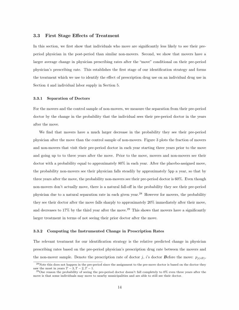
We find that movers have a much larger decrease in the probability they see their pre-period

physician after the move than the control sample of non-movers. Figure 3 plots the fraction of movers

and non-movers that visit their pre-period doctor in each year starting three years prior to the move

and going up to to three years after the move. Prior to the move, movers and non-movers see their

doctor with a probability equal to approximately 80% in each year. After the placebo-assigned move,

the probability non-movers see their physician falls steadily by approximately 5pp a year, so that by

three years after the move, the probability non-movers see their pre-period doctor is 60%. Even though

non-movers don’t actually move, there is a natural fall-off in the probability they see their pre-period

physician due to a natural separation rate in each given year.28 However for movers, the probability

they see their doctor after the move falls sharply to approximately 20% immediately after their move,

and decreases to 17% by the third year after the move.29 This shows that movers have a significantly

larger treatment in terms of not seeing their prior doctor after the move.

3.3.2 Computing the Instrumented Change in Prescription Rates

The relevant treatment for our identification strategy is the relative predicted change in physician

prescribing rates based on the pre-period physician’s prescription drug rate between the movers and

the non-mover sample. Denote the prescription rate of doctor j, i’s doctor Before the move: pj(iB),

28Note this does not happen in the pre-period since the assignment to the pre-move doctor is based on the doctor theysaw the most in years T � 3, T � 2, T � 1.

29One reason the probability of seeing the pre-period doctor doesn’t fall completely to 0% even three years after themove is that some individuals may move to nearby municipalities and are able to still see their doctor.

14

and denote the prescription rate of doctor j0, i’s doctor After the move: pj(iA).30 We want to estimate:

E(pTj(iA)� pT

j(iB)|pTj(iB))�E(pCj(iA)� pC

j(iB)|pCj(iB)) - the difference in conditional expectations based on

the pre-period physician’s prescribing rate between the treatment and control sample.

To calculate this, we first calculate the change in physician prescription drug rates of their post-

period and pre-period doctor for every individual in the mover and non-mover sample. We then plot

the relationship between the change in prescribing rates and the pre-period physician’s prescribing rate

in Figure 4A, by binning the pre-period physician’s prescribing rate of opioids into 20 equal size bins,

and plotting the average change in physician’s prescribing rate for each bin. The light red diamonds

and fitted line show the relationship between the change in physician’s opioid prescribing rate and the

pre-period physician’s opioid prescribing rate for the movers, while the dark blue dots and line show

the relationship for the non-movers.

This figure shows that for movers, the change in physician’s opioid drug rate is on average equal

to -.75 of their old physician’s prescription drug rate. The R2 for the comparable regression is .39. If

there was perfect sorting of individuals to their new physician based on their old physician prescribing

rate, we would expect a coefficient of 0, if there was no sorting and perfect mean reversion, we would

expect a coefficient of -1. The coefficient of -.75 suggests that there is some sorting of individuals into

new physicians based on their old physician’s prescribing rate, but the mean reversion effect is very

strong.

For non-movers, the pre-period’s physician drug rate is also predictive of the change in pre-

scription drug rate, but the gradient is much flatter - the change is approximately -.22 of the pre-

period physician’s prescription drug rate. This is not equal to zero because some of non-movers

separate from their physician and have some mean reversion in their choice of new physicians as

well. Therefore, the relative treatment for the movers compared to the non-movers is the difference:

(�.75� .22) ⇤ pj(iB) = �.53 ⇤ p

j(iB). Figure 4 Panels B-D show that the results for the other drugs are

very similar.

Formally, for each type of prescription drug, we estimate the relative predicted difference of the

change in prescription drug rates using the following regression equation:

pj

0(iA) � pj(iB) = �0 + �1p

j(iB) + �2Moveri

+ �3pj(iB) ⇥Moveri

+ ✏i

(2)30We use a leave-out procedure so that pj(iB) and pj(iA) are not calculated using individual i’s own prescription drug

use.

15

We calculate the relative predicted difference in the change of prescription drug rates as the product

�3 and the previous physician’s prescription drug rate: �j(i) = �3p

j(iB). Table 1 row 3 reports the

standard deviation of �j(i) for each drug. For opioids, the standard deviation in the relative treatment

is .9 percentage points. While it is smaller than the total variation in physician prescription rates, it is

still substantial. The variation for the other drugs is slightly higher, with anti-inflammatories having

the largest at 1.5 percentage points.

4 Effect of Physician Prescribing Rates on Drug Use

This section describes and implements the methodology we use to identify the effect that physician’s

prescribing rates have on individual’s prescription drug use. We find that physicians have a significant

causal impact on individual’s prescription drug behavior.

4.1 Estimating Equation for Impacts of Moves on Prescription Drug Use

To identify the effects of physician prescribing rates on individual’s drug use, we use the following

identification equation

Drugit

= ✓r(i,t)�p(i) ⇥Mover

i

+ �r(i,t)�p(i) + r(i,t)Mover

i

+ µo,d,r

+ ✏it

(3)

Where �p(i) is the relative predicted change in physician prescription drug rates between the mover

and non-mover sample based on the pre-period physician’s prescribing rate, and µo,d,r

are origin by

destination by year relative to move fixed effects, which control for location based effects. Drugit

is

an indicator (0 or 1) for whether individual i purchases the drug in year t. �p(i) ranges approximately

from -.04 to .04 - such that �p(i) = .02 would indicate that there was a predicted relative change of

2pp in the physician prescribing rates. ✓r(i,t) is a flexible function allowing for separate coefficients on

�p(i) for each year relative to the move. We normalize ✓�1 equal to zero so that the other coefficients

indicate the effect of �p(i) relative to the year prior to the move. Thus ✓

s

estimates the triple difference

effect - the effect of the predicted change in physician prescription drug rates, for movers relative to

non-movers, and in year s relative to the year prior to the move on individual’s own prescription drug

use. For ease of description, we sometimes refer to ✓s

as the effect of a change in physician prescription

drug rates in year s relative to the year prior to the move.

The specification assumes that there is a linear effect of the change in physician prescribing rates

16

on individual’s prescription drug use. In Appendix E, we allow there to be a non-parametric affect of

the change in physician prescribing rates on drug use and find that our linear choice is justified.

We include observations for up to three years prior to the move and three years after the move, for

the years 1995-2015 and individuals aged 30-70. Note that this is not a balanced sample by individual

and year relative to move; however, due to the exact match between the treatment and control group

on age and year, each sample is unbalanced in the same way.

4.2 Results

We find that an increase in physician prescribing rates of opioids increases individual’s own prescription

drug use, suggesting that physicians have a causal effect on their patients’ use of prescription opioids.

Figure 5 plots the coefficients (✓r(i,t)) on the instrumented change in physician prescription rates (�

p(i))

for the mover sample, relative to the non-moving sample for each year relative to the year prior to the

move. Panel A depicts the results for opioids and shows that in the year of the move, movers’ drug use

starts increasing with respect to the change in physicians’ prescribing rates relative to the response of

non-movers. It continues to increase until the year after the move at to a coefficient of approximately

.4.31

One concern is that time-varying selection biases our results. If this were the case, we would expect

to see that the correlation between individual’s drug use and the change in physician prescribing rates

to increase prior to the move. In fact, there is no trend prior to the move, indicating that the change

we see at the time of the move is unlikely to be due to time-varying selection. We may still worry that

the relationship between concurrent health shocks and the pre-period physician’s prescription drug

rates is different for the movers than for the non-movers. Particularly, we would worry that movers

who have low-prescribing opioid doctors are more likely to have a concurrent “bad” health shock than

individuals who do not move, and movers who have a high-prescribing opioid doctors are more likely

to have a “good” health shock than the individuals who do not move.

To check if differential simultaneous shocks are a problem, we look at the relationship of prescription

drug use and the change in physician prescribing rates by months since the move. We run the following

regression:

Drugim

= ✓r(i,m)�p(i) ⇥Mover

i

+ �r(i,m)�p(i) + r(i,m)Mover

i

+ µo,d,r

+ ✏im

, (4)31There is a partial response in the year of the move because on average individuals will spend half of that year in the

new municipality.

17

where ✓r(i,m) are indicators for months since the move and range from 6 months before the move to

6 months after the move, Drugim

is an indicator for whether individual i ever took the prescription

drug in month m (rather than within a year), and µo,d,r

are destination by origin by month relative to

move fixed effects. �p(i) is the same instrumented change in physician prescription drug rates based

on the pre-period physician’s prescribing rate.32

Figure 6 plots ✓r(i,m) by the month since the individual moved for each drug. Panel A plots the

coefficients for the outcome of opioid use and the treatment of physician opioid prescriptions. While

the coefficients are substantially noisier than the annual coefficients, they also show a flat trend prior

to the move, and a distinct increase right at month zero - the month of the move. The fact that the

response is immediate at the month of the move provides evidence that this is a causal effect of the

move rather than due to correlated concurrent health shocks.

We have shown that these results are unlikely to be driven by differential health trends or shocks.

To aggregate the results into one coefficient we estimate:

Drugit

= ✓Afterit

⇥�p(i)⇥Mover

i

+�After⇥�p(i)+ After

it

⇥Moveri

+µo,d,r

+�1�p(i)+�

r(i,t)Xit

⇥Moveri

+✏it

(5)

In Table 1, we report ✓, which estimates the average effect of the instrumented change in prescription

drugs of the movers relative to the non-movers in the three years after the move versus the three years

prior. In column (1) we report the results for opioids and find that an individual’s drug use increases

by .48pp for a 1 percentage point increase in their physician’s prescription drug rate, with a standard

error of .03pp.33 This indicates that 48% of the variation in physician residualized prescription opioid

drug rates is driven by the doctor rather than differences in demand of their patients.34

Since the physician prescription drug rates are already residualized with respect to individuals age,

gender, and education, to calculate the percent of the total variation in physician prescribing rates that

is due to causal physician effect, we do the following calculation: sd

2R

sd

2tot

⇥ .48 = 1.82

2.32 ⇥ .48 = .29. Where

sd2R

is the squared standard deviation of the residualized physician opioid prescribing rate (Table 1

Row 2), and sd2tot

is the squared standard deviation of the total raw physician prescribing rates (Table

1 Row 1). This calculation shows that 29% of the total variation in physician prescribing rates is due32Note, however, that the physician prescribing rates are still in annual units: the fraction of their patients that took

the prescription drug within the year. This means that the coefficients ✓r(i,m) are not on an equivalent scale as ✓r(i,t).33Another way to interpret the magnitudes coefficient is to put it in terms of standard deviation effects: a one standard

deviation increase in physician prescribing rates of opioids leads an individual to increase their own prescription druguse by .8 pp, or 12% of the mean opioid use.

34This is not equal to 100%, since the residualized physician prescribing rate still includes variation due to differencesin demand of their patients based unobservable differences in health.

18

to causal physician effects.

Figure 5 Panels B-D show the results for the prescribing rates of anti-inflammatories, anti-anxieties,

and anti-depressants respectively. They all show a flat trend prior to the move and a strong significant

increase after the move. The magnitudes of the increase vary slightly, but they all show a significant

response with coefficients between .35 and .6. When we look at monthly prescription drug use in the six

months before the move and six months after the move for these drugs in Figure 6 Panels B-D, we see

that there are no differential pre-trends in the monthly leading up to the move for anti-inflammatoris,

anti-anxietes, and anti-depressants either. Additionally, all show an impact on drug use from the

change in prescribing rates in the month of the move providing evidence that the effect of the change

in physician prescribing rates on individual’s prescription drug use is causal.

In Table 2 columns 2-4, we report ✓, from Equation 5, the average effect of the instrumented change

in prescription drugs of the movers relative to the non-movers in the three years after the move versus

the three years prior. For anti-inflammatories: a 1pp increase in the physician prescribing rate leads

to a .58pp increase in individual’s probability of taking anti-inflammatories. For anti-anxieties: a 1

pp increase in the anti-anxiety prescribing rate leads to a .36pp increase in the probability of taking

anti-anxieties. And for anti-depressants: 1 pp increase in the anti-depressant prescribing rate leads to

a .47pp increase in the probability of taking anti-depressants.35

4.3 Heterogeneity In Treatment Impacts by Individual Characteristics

To understand the distributional implications of the variation in physician prescribing rates, we need to

know which individuals are the most influenced by their physicians. To do so, we estimate heterogenous

effects of physician prescribing rates on prescription drug use by gender, age, education, and whether

individuals work in blue collar occupation. We find a substantial amount of variation in the effects by

these characteristics especially for prescription opioid use.

We turn age and education into binary variables based on whether the individual’s level of a given

variable is above or below the median at the time of the move.36 We create an indicator for whether an

individual worked in a blue collar occupation based on their occupation four years prior to the move.

To estimate heterogenous effects by each characteristic, Xi

, we first reestimate �p(i), the relative

35In terms of standard deviation units: a one standard deviation increase in physician anti-inflammatory prescribingrates leads to a 1.7pp or a 8.8% increase in anti-inflammatory prescription drug use. A one standard deviation increasein physician anti-anxiety prescribing rates leads to a .9pp or a 12% increase in anti-anxiety prescription drug use. A onestandard deviation increase in physician anti-depressant prescribing rates leads to a .8pp or a 10% increase in prescriptionanti-depressant use.

36The median age is 42 and the median education level is 14 years of education.

19

predicted change in physician prescribing rate based on their pre-period physician’s prescription rate

for movers compared to non-movers, as a function of Xi

. We do this because individuals with different

characteristics may have different amounts of mean reversion from the pre-period to their post-period

physician prescribing rate.

Since each Xi

is binary, we simply estimate:

pj(iA) � p

j(iB) = �00 + �0

1pj(iB) + �02Mover

i

+ �03pj(iB) ⇥Mover

i

+ ✏i

8i s.t. Xi

= 0 (6)

pj(iA) � p

j(iB) = �10 + �1

1pj(iB) + �12Mover

i

+ �13pj(iB) ⇥Mover

i

+ ✏i

8i s.t. Xi

= 1 (7)

Where �j(i) is the change in physician prescribing rates: p

j(iA) � pj(iB). We then create the new

instrumented variable as a function of Xi

: �p(i)i = �0

3(1�Xi

)⇥ pj(iB) + �1

3Xi

⇥ pj(iB), and estimate

the following equation to identify heterogeneous effect of physician’s prescribing rates on individual

use:Drug

it

=✓1After ⇥ �p(i)i ⇥Mover

i

⇥Xi

+ �1After ⇥ �p(i)i ⇥X

i

+

1After ⇥Mover ⇥Xi

+ �1Mover ⇥Xi

+ �1�p(i)i ⇥X

i

+

✓0After ⇥ �p(i)i ⇥Mover

i

+ �0After ⇥ �p(i)i+

0After ⇥Mover + �0Mover + �0�p(i)i + µ

o,d,r,X

i

+ ✏it

(8)

✓1 estimates the difference between the effect of a change in physician prescription drug rates for

individuals with characteristic Xi

compared to those without Xi

, while ✓0 estimates the base effect of

the change in physician prescription drug rates for those without characteristic Xi

. We also include

origin by destination by after by characteristics fixed effects (µo,d,r,X

i

) to control for the possibility that

individuals with different Xi

are differentially influenced by location effects as well. Table 3 reports

the estimates for ✓1 and ✓0 with Column 1 showing heterogeneity by age (Xi

= agei

> 42), Column

2 by gender (Xi

= femalei

), Column 3 by education (Xi

= Y earsEduci

> 14), and Column 4 by

occupation (Xi

= BlueCollari

).37

We find that individuals who are older, female, less educated, or worked in blue collar occupations

have a significantly larger effect of a change in their physician’s opioid prescribing rate on their own

opioid prescription drug use. Table 3 Panel A reports the coefficients for opioids, and shows that older

individuals have a 75% larger response than younger individuals; women have a 60% larger response

than men; less educated individuals have a 75% larger response than more educated individuals; and37Where 42 is the median age, and 14 is the median years of education in the sample.

20

blue collared workers have a 89% larger response than white collared workers. Tables 3 Panels B-D

show the results for anti-inflammatories, anti-anxieties, and anti-depressants respectively. For anti-

inflammatories, we find that those with less education are more affected by their physician’s prescribing

rate. For anti-anxieties in Table 3 Panel C, we see that older workers, women, and blue collar workers

are more likely to be affected by their physician prescribing rate. For anti-depressants in Table 3 Panel

D, we find that women and blue collar workers have a larger effect.

Generally, we find that differences in the effects align with the differences in the exante probability

individuals use the drug. Appendix Table 2, Panels A-D report the difference in probabilities of

prescription drug use for individuals with these different characteristics for the different prescription

drugs we study. Those who are more likely to use the drug are also more likely to be affected by the

change in physician prescribing rates.

5 Effect of Physician Prescribing Rates on Labor Outcomes

In this section, we estimate the effect of physician prescribing rates on individual’s labor supply out-

comes. We first present the main results, which look at the effects on labor income rank. Next, we

show the effects on additional labor outcomes: labor force participation, log labor income, labor in-

come rank defined for individuals with positive labor income, two sick pay measures, and Disability

Insurance receipt. Finally, we show that individuals who move farther distances and have a larger

change in prescribing rates also have bigger changes in labor supply. This provides additional evidence

that the labor supply effects come from the change in the physician’s prescribing rate rather than

other confounding factors. In Appendix F, we also estimate whether there are heterogenous effect for

individuals by their age, gender, education, and occupation; however, due to large standard errors, it

is difficult to make any strong conclusions.

5.1 Estimating Equation for Effects of Physician Prescribing Rates on La-

bor Income

Similar to our estimation of the effects of physician prescription rates on drug utilization, our equation

for identifying the effects of a change in physician prescribing rates on labor income is the following:

LaborIncomeit

= ✓Lr(i,t)�p(i) ⇥Mover

i

+ �Lr(i,t)�p(i) +

L

r(i,t)Mover + µL

o,d,r

+ ✏it

(9)

21

Where �p(i) is the predicted relative change in physician prescription drug rates based on the pre-

period physician’s prescribing rate (calculated in Section 3.3.2), and µL

o,d,r

are origin by destination by

year relative to move fixed effects, which control flexibly for local labor market effects of the origin and

destination. ✓Lr(i,t) is a flexible function allowing for separate coefficients on �

p(i) for each year relative

to the move. We normalize ✓�1 equal to zero so that the other coefficients indicate the effect of �p(i)

relative to the year prior to the move. Thus, just like in section 4.1, ✓Ls

estimates the triple difference

effect - the effect of the predicted change in physician prescription drug rates, for movers relative to

non-movers, and in year s relative to the year prior to the move on individual’s labor income.

The primary outcome variable we consider is labor income rank because it includes both the

extensive and intensive margin responses. In section 5.2.2, we look at the effect of physician prescribing

rates on other labor market outcomes to see if the effects are robust to different measures and to identify

whether the results are driven primarily by the extensive or intensive margin response.

5.2 Results

5.2.1 Results on Labor Income Rank

Opioids: We find that an increase in physician opioid prescribing rates leads to a decrease in individ-

ual’s labor income. Figure 7 plots the coefficients (✓Lr(i,t)) on the instrumented change in physician

prescription rates (�p(i)) for the moving sample relative to the non-moving sample for each year rela-

tive to the year prior to the move. Panel A shows the results for the effect of opioid prescribing rates

on labor income rank. It shows that in the year of the move, mover’s labor income rank starts to

decrease with respect to the change in the physician’s opioid prescribing rate relative to the response

of non-movers. It continues to decrease until the year after the move at which point it levels off. Prior

to the move, there is no significant trend, which means that individuals who move do not change their

labor supply in response to the change in their physician’s opioid prescribing rate prior to the move

relative to the non-mover sample. This suggests that the large change we see at the time of the move

is unlikely to be due to time-varying selection. Table 4 Panel A reports the estimates for the effect

of the predicted change in physician opioid prescription rates in the three years after the move versus

the three years prior to the move, clustering the standard errors at the individual level. Column (1)

reports that a 1pp increase in the opioid physician prescription rate is associated with a .11 percentile

decrease in labor income rank.

Because we might be concerned that individuals may move for different reasons and have different

22

effects of the move, Figure 7 Panel B show that the results do not change when we include controls to

allow for individuals with different pre-characteristics to have different effects of the move. Specifically,

we include year since the move fixed effects interacted with an indicator for mover, and separately

interacted with the following: a quadratic in age, gender, and the full set of interactions of years of

education, average labor income rank from T � 8 to T � 4, and age. We find that when we add these

controls, there is little change in the results. Table 4 Column (2) reports the aggregated effect of a

1pp change in physician prescribing rates after the move versus before with these controls as a .12

percentile decrease in labor income rank, which is statistically significant at the 5% level.

Anti-Inflammatories: Figure 8, Panel A plots the results for anti-inflammatory prescribing rates,

and Panel B plots the coefficients for the regression that includes controls allowing for heterogenous

effects of the move for individuals with different observable pre-characteristics. We find no significant

effects for a change in physician anti-inflammatory prescribing rates on labor income rank in either

specification. There is maybe a small decrease in the year after the move, but it is not quite statistically

significant at the 5% level. Table 4 Panel B, Column (1) and Column (2) report the estimates for the

aggregated effect after versus before and finds coefficients of 0.033, with a standard error of .023 and

-.035, with a standard error of .02, neither of which are statistically significant at the 5% level.

Anti-Anxieties: For anti-anxieties (Figure 9 Panels A and B), we find no discernible effect of

physician anti-anxiety prescribing rates on labor income rank with or without controls for individual

pre-characteristics. Again, there is perhaps a small decrease in the year after the move that is just

barely significant at the 5% level, but when we control for differences in individual pre-characteristics,

this effect attenuates and becomes statistically insignificant. Table 4 Panel C, Column (1) reports

the coefficient for the aggregated effect of after versus before as -.088 with a standard error of .028

without controls. Once we include controls for heterogeneity in the effects of the move by individual

characteristics in Column (2), this coefficient becomes -.035 with a standard error of 0.02 and is no

longer statistically significant at the 5% level.

Anti-Depressants: In Figure 10 Panels A and B, we plot the effects of physician anti-depressant

prescribing rates on labor income rank, with and without controls for previous individual character-

istics. They show that an increase in the physician prescribing rate of anti-depressants leads to a

decrease in labor income rank. While not significant, the pre-trends are not entirely flat, which may

suggest that some of the effect is due to differential trends for movers and non-movers with respect to

the predicted change in the physician prescribing rate of anti-depressants. Aggregating the coefficients

23

from after and before in Table 4, we find that without controls a 1 pp increase physician prescribing

rates of anti-depressants is associated with a decrease of .15 percentiles in individual’s labor income

income rank, with a standard error of .036. When we add controls for individual characteristics in

Column (2) and Figure 10 B, the effect decreases in magnitude to .11, but stays statistically significant

at the 5% level. However, this difference includes changes in the pre-period so it is unlikely to reflect

a causal effect.

Horse-Race: In the above analysis, we looked separately at the effect of physician prescribing rates

of different drugs. However, physician’s prescribing rates for different drugs are highly correlated with

each other. Table 5 reports the correlation between the different physician prescribing rates, as well as

the correlation between the specific treatments we use in our analysis - the relative predicted change in

physician prescribing rates. The correlations range between .23 and .57. The highest correlations are

between physician opioid prescribing rates and the prescribing rates of the other drugs. For example, for

the correlation between th predicted relative change in physician prescribing rates of opioids and anti-

depressants is .57, while for opioids and anti-anxieties it is .48, and for opioids and anti-inflammatories

it is .43. Because the treatments are correlated, it is unclear whether the estimated effects on labor

income is due to the specific prescribing rate or due to it’s correlation with the other prescribing rates

To separate out the specific effects of each physician prescribing rate, we control simultaneously for

them in the same regression. The interpretation of these coefficients, for example, is the effect of

having a physician that has a higher opioid prescribing rate holding fixed their prescribing rate of

anti-inflammatories, anti-anxieties, and anti-depressants.

Figure 7 Panel C, shows that for opioids there is similar sized effects when we additionally control

for the other prescribing rates of drugs. On the other hand, Figure 8 Panel C shows that any small

decrease in labor income that was associated with an increase in inflammatory prescribing rates is gone

once we include controls for the other prescribing rates. Figure 9 Panel C shows the results for anti-

anxiety prescribing rates and shows that once we control for the other prescribing rates, an increase

in the anti-anxiety prescribing rate is associated with a small increase in labor income - though none

of the point estimates are statistically significantly different from zero at the 5% level. Finally, Figure

10 Panel C shows that once we control for the other prescribing rates, the effect of increase in the

physician prescribing rates of anti-depressants on labor income is no longer significant.

In Table 4 Column 3, we report the estimates of the aggregate effect of the relative instrumented

change after versus before the move when we control for the other prescribing rates for each type

24

of drug. We find that a 1 pp increase in opioid prescribing rate leads to a -.12 (se=.05) percentile

decrease in labor income rank; a 1 pp increase in the anti-inflammatory prescribing rate leads to a

-.002 (se=.022) percentile change in labor income rank; a 1 pp increase in the anti-anxiety prescribing

rate leads to a .055 (se=.035) percentile change in the labor income rank, and a 1pp increase in the

anti-depressant prescribing rate leads to a -.077 (se=.038) percentile change in labor income rank.38

Note that for anti-depressants, that the coefficient is significant, but this is again likely due to the

pre-trend we see in Figure 10 Panel C. Therefore, this estimated effect is unlikely to be causal.

We conduct a test to see if the opioid effect is statistically significantly different than the other

effects. We find that the p-value for opioids and anti-inflammatories to have the same effect is .03, for

opioids and anti-anxieties to have the same effect is .003, and for opioids and anti-depressants to have

the same effect the p-value is .0008. This provides evidence that the prescribing rates of opioids have

a negative effect on labor income rank, while the other drugs have smaller or no effects.

5.2.2 Other Labor Outcomes

To understand the effect that physician prescribing rates have on labor supply more completely, we

look at the effects on other labor supply measures: labor force participation, log labor income, labor

income rank for individuals with positive labor income, two measures of receipt of sick pay, and

receipt of disability insurance. We find that physician’s prescribing rate of opioids has a negative and

significantly significant impacts on individual’s labor force participation and their log labor income,

while the prescribing rates for the other drugs have no significant effects on any of the additional

outcomes we look at.

Table 6 shows the results of the effects of physician opioid prescribing rates when these different

measures are the outcome variables. We include observations from three years prior to the move and

three years after the move, not including the year of the move, and estimate the following equation,

where Yit

, is the outcome variable of interest:

Yit

= ✓Afterit

⇥�p(i)⇥Mover

i

+�After⇥�p(i)+ After

it

⇥Moveri

+µo,d,r

+�1�p(i)+�

r(i,t)Xit

⇥Moveri

+✏it

(10)

We report the coefficient, ✓, on the interaction with an indicator for After, the predicted relative38To compare the effect that physician prescribing rates have on labor income once we control for all the prescription

drug rates simultaneosly to the effect they have on prescription drug use, we rerun the regressions of prescription druguse for each drug on the full set of physician prescribing rates. These results are reported in Appendix Table 3. Column1 shows that the coefficient on the opioid physician prescribing rate in the regression on opioid drug use is .61.

25

change in physician prescribing rates, �p(i), and the indicator for Mover.

In Table 6, we include the same set of controls as Table 4 Column 3, controlling flexibly for

differences between individuals and for the physician prescribing rates of other drugs. In Appendix

Table 4, we show the results for when we include controls for differences between individuals, but

not other prescribing rates. For each column, we run equation (10) on a different outcome variable.

Column (1) reports the results for labor income rank (replication of Table 4 Column 3), Column (2)

reports the results on labor force participation (either equal to 0 or 1), Column (3) reports the results

on ln(LaborIncome+ 1), Column (4) reports the results on labor income rank defined for individuals

with positive labor income (ranges from 0 to 1), Column (5) reports the results on an indicator for

receiving sick pay within a year (either 0 or 1), Column (6) reports the results on an indicator for

receiving sick pay for more than four weeks (either 0 or 1), and Column (7) reports the results on DI

receipt (either 0 or 1).

Panel A shows the results for the effect of physician prescribing rates of opioids on various labor

supply measures. We find that there is large negative and statistically significant effects on labor force

participation and log labor income: a 1 percentage point increase in physician’s opioid prescribing rate

leads to a -.2 percentage point decrease in labor force participation, and a 2.3% decrease in log labor

income. For the other outcomes, there are not statistically significant effects, but the point estimates

go in the same direction as the results on labor income rank, labor force participation, and log labor

income. Specifically, a one percentage point increase in physician opioid prescribing rates is associated

with a -.065 (se=.048) percentile decrease in labor income rank for those with positive labor force

participation, a .05 (se=.08) percentage point increase in probability of receiving any sick pay, a .15

(se=.08) percentage point increase in the probability of receiving more than two weeks of sick pay, and

a .01 percentage point increase in probability receive DI.

These result suggests that the prescribing rate of opioids affects the extensive margin of labor

supply, but it is unclear how important the effect on intensive margin is. The point estimate for

the regression of labor income rank for those with positive labor force participation (.065) suggests

that approximately half of the total effect on labor income rank (.12) is due to the intensive margin;

however, the standard errors are large enough that we cannot rule out that there is no effect on the

intensive margin of labor supply.

Panels B-D show the results for anti-inflammatories, anti-anxieties, and anti-depressants. We find

no statistically significant effects on any of these other outcomes for any of the other drugs. For

26

anti-anxieties, we continue to see positive effects on labor supply measures, but none of them are

statistically significant at the 10% level. Importantly, for anti-depressants, even though there was a

statistically negative effect on labor income rank (likely due to pre-period trends), we do not see any

statistically significant effects on the other outcomes. The point estimate on labor force participation,

labor income, and labor income rank conditional on positive participation, as well as DI point towards

a negative effect on labor supply, though the effects on sick pay point toward a small positive effect.

5.3 Heterogeneity in Treatment Effects by Distance of Move

As a robustness check, we test for heterogeneity in the effect by distance of the move. Individuals who

move longer distances are more likely to separate from their prior physician and thus have a larger

change in prescribing rates. We therefore test whether they also have stronger effects on their drug

use and labor supply, since this would provide evidence that the changes in labor supply and drug

use are directly related to the changes in physician prescribing rates rather than differences in the

effect of move for different individuals. Specifically, this relaxes the assumption that the correlation

between the change in unobservables and individuals prior physician’s prescribing rate is the same for

individuals who move and do not move, and instead assumes that the correlation between the change in

unobservables and individual’s prior physician’s prescribing rate is the same for individuals who move

different distances. We find results that are consistent with our previous estimates, which suggests

that the effects we see on labor income are due to the changes in physician prescribing rates.

Our distance measure is the change in probability other individuals who move between the same

two municipalities see their pre-period physician after the move. This estimated separation rate we

call: si

. To show that this distance measure affects the first stage, we bin the separation rate into 20

equal sized bins and estimate the coefficients in the following equation:

pj(iA) � p

j(iB) = ↵+20X

b=0

(�b

pj(iB)Is

i

2bin

b

+ ⇡b

Is

i

2bin

b

) + ✏i

(11)

Where pj(iB) is the individual’s physician’s prescription rate prior to moving, and I

s2bin

b

is an indicator

variable for whether the estimated separation rate from i’s move is within binb

. Figure 11a plots the

coefficients �b

by the mean value of the separation rate in binb

for prescribed opioids and shows a clear

relationship between the magnitude of the change in prescription drug rates and the probability that

individuals separate from their previous physician based on their origin and destination municipality.

27

To now understand how this affects an individual’s probability they use the prescription drug, we

estimate the following equation:

Drugit

= ↵+TX

b=0

(�b

pj(iB)Is

i

2bin

b

+ ⇡b

Is

i

2bin

b

) +TX

b=0

(µb

pj(iB)Is

i

2bin

b

Afterit

+ ⇢b

Is

i

2bin

b

Afterit

) + ✏i

(12)

Since we previously found that individuals with certain characteristics had different effects of the move

and the change in physician prescribing rates, we also allow for heterogeneity in the effects by age,

gender, education, and previous blue collar status.

The coefficients of interest are µb

,which are the coefficients on the interaction of the previous

physician’s prescribing rate, an indicator for the separation rate being in bin b, and an indicator of

after. They show how the relationship between the change in individual’s prescription drug use and

the pre-period physician’s prescribing rate changes for different bins of the separation rate.

Figure 11b plots µb

by the mean value of si

in binb

for opioid prescription drug use. The figure shows

that the relationship between the change in individual’s drug use and the prior physician prescribing

rate decreases for longer distance (ie higher separation rate) moves. Given that relationship between

the change in physician prescribing rate and the previous physician’s prescribing rate also decreases

with longer distance moves (Figure 11a), this finding supports the evidence from Section 4.2, except

here, instead of comparing the response between non-movers and movers, we compare the response

between individuals who are more or less likely to be separated from their physician based on the

distance of the move.

Now we move to the effect on labor income rank. We estimate the following equation:

LaborIncomeit

= ↵+TX

b=0

(�b

pj(i)⇥I

s

i

2bin

b

+⇡b

Is

i

2bin

b

)+TX

b=0

(µb

pj(i)⇥I

s

i

2bin

b

⇥Afterit

+⇢b

Is

i

2bin

b

⇥Afterit

)+✏i

(13)

Figure 11c plots µb

by the mean value of si

in binb

for opioid prescription drug use. The figure shows

that the relationship between the change in individual’s labor income after the move and the prior

physician prescribing rate increases for longer distance moves. Since the longer distance moves led to a

larger decrease in the physician prescribing rates, this suggests that a decrease in physician prescribing

rates of opioids leads to an increase in labor income rank. In Figure 11d we additionally include the

physician prescribing rates of the other drugs and find little effect on the results. This supports the

evidence from Section 5.2.

28

In Appendix Figures 6-8, we show a similar set of plots for anti-Inflammatories, anti-Anxieties,

and anti-Depressants. For each drug we find that larger distance moves leads to larger changes in

physician prescribing rates, and a larger change in individuals own prescription drug use for a given

level of pre-period physician’s prescribing rate. Appendix Figure 6, Panels C and D show that longer

distance moves have no effect on the relationship between prior physician inflammatory prescribing

rates and the change in labor income rank, whether or not we include controls for the other prescribing

rates (Panel D) or do not (Panel C). Appendix Figure 7 Panel D shows that once we include controls

for the other prescribing rates, a longer distance move leads to a smaller relationship between the prior

physician’s anti-anxiety prescribing rate and labor income. This is inline with the results from Section

5.2 and Figure 9c. For anti-depressants, in Appendix Figure 8 Panels C and D we see that longer

distance moves leads to larger decreases in labor income, though the relation is fairly noisy once we

include controls for the other prescribing rates.

6 Conclusion

In this paper, we show the effects of a change in physician prescribing rates of four important and

widely used classes of drugs used to treat musculoskeletal and mental health disorders (opioids, anti-

inflammatories, anti-anxieties, and anti-depressants) on a variety of outcomes. We find that a one

percentage point increase in physician prescribing rates leads to an increase of approximately .45

percentage points in individual’s own usage of the prescription drug. From this, we calculate that

approximately 30% of the total variation in physician prescribing rates is due to causal physician

effects rather than selection of patients. We find that generally individuals who are older, who are

women, who are less educated, and work in blue collar occupation have larger effects of physician

prescribing rates on their own prescription drug use, but there is some heterogeneity by the specific

drug.

When we look at labor market outcomes, we find that an increase in physician’s opioid prescribing

rate leads to a decrease in individual’s labor income and labor force participation: a 1 percentage point

increase in physician’s opioid prescribing rate leads to a decrease of .12 percentiles of labor income

and .15 percentage point decrease in labor force participation. We do not find consistent effects of

physician prescribing rates of the other drugs on labor supply outcomes.

So far we have been careful not to attribute the labor supply effects directly to the effects on the

changes in prescription drug use. This is because while physician prescribing behaviors do strongly

29

effect individual drug use, the prescribing rates may be correlated with many other physician traits

that also help determine labor supply. However, we now discuss our results under the possibility that

the effects we see are caused by prescription drug use, to better understand the implications of this

interpretation.

If we control for the other physician prescribing rates, remember that a 1pp increase in the physician

prescribing rate of opioids led to a .6pp increase in opioid use and a .12 decrease in labor income rank

and a .2 decrease in their labor force participation. If we make the interpretation that physician

prescribing rates affect labor income only through their effect on prescription drug use, then our

estimates that control for the prescribing rates of other drugs suggest that if an individual went from

not prescription opioids to taking prescription opioids, we would expect their labor income rank to

decrease by 20 percentiles and their labor force participation to decrease by 33 percentage points.39

As a comparison, Boscarino et al. 2010 find that an estimated one fourth of out-patients on opioid

chronic pain therapy develop opioid dependence. Granted that the increase in usage may be for a short

period and not necessarily in long term chronic pain therapy, and since not all opioid dependence would

necessarily lead to a drop out of the labor force, we might expect a smaller effect. Given that opioid

prescribing rate may be correlated with other physician characteristics, we think of this estimate as

an upper bound of the negative effect opioids have on labor supply.

For this interpretation, it is also important to note that we estimate a local treatment effect for indi-

viduals who are influenced by their physician’s prescribing rate. This may be a particularly important

caveat for interpreting the effects of anti-depressants. While we might expect anti-depressants to have

a positive effect on labor income, as they clinically have been shown to alleviate depression - which can

be debilitating,40 we find some results which suggest that they have a negative effect on labor supply

or no effect.41 However, during the time period we study, anti-depressants grew tremendously such

that by 2010, 10% of the working population took them. In the United States, where anti-depressant

use has also increased dramatically, a recent study showed that nearly 2/3 of patients diagnosis with

depression were given a false positive diagnoses, and the vast majority were given medication (Mojtabi

2013). This suggests that the prescribing rate is at a level such that the marginal patient does not

benefit from anti-depressant medication.39Note that this requires a large amount of extrapolation: a one standard deviation increase in physician prescribing

rates of opioids leads only to a 1.1 percentage point increase in individual’s own prescription opioid use.40Note that the one medical control trial that we know of that randomly assigned an anti-depressant or a placebo and

looked at labor outcomes (N=43) found a negative effect on hours worked in the 6 weeks of follow-up, but it was notstatistically significant (Agosti, Stewart, and Quitkin 1991).

41Note that due to large standard errors we cannot rule out some positive effect.

30

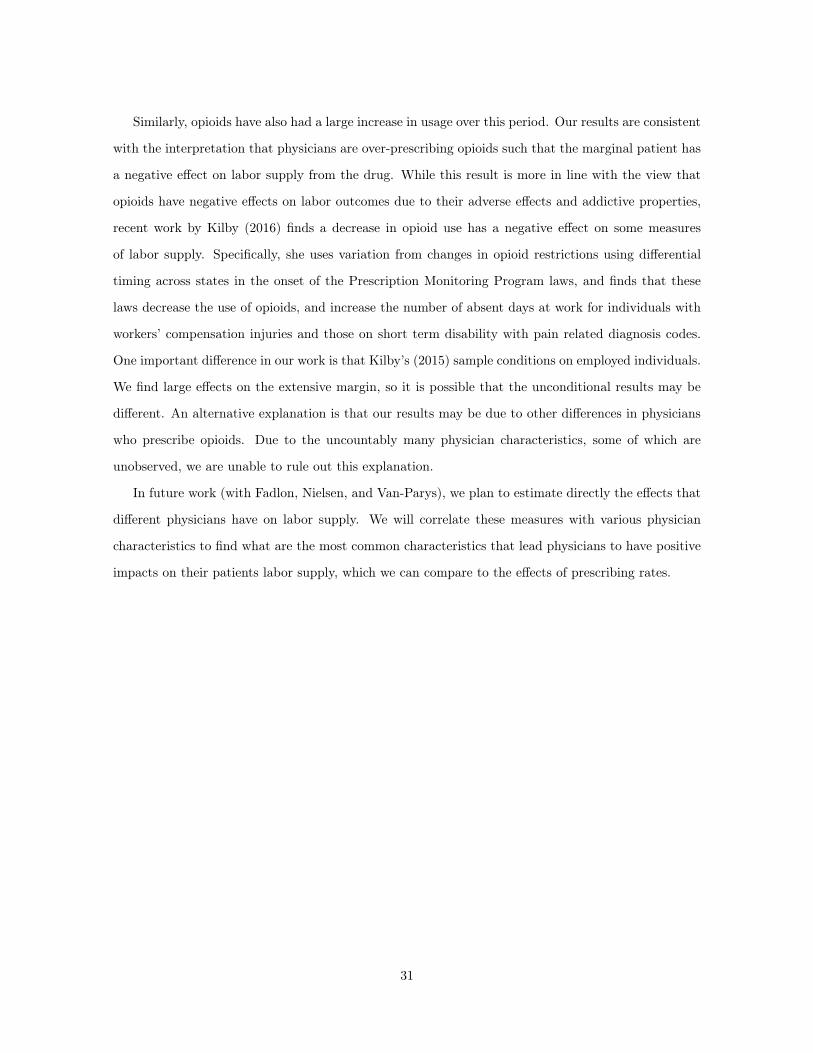
Similarly, opioids have also had a large increase in usage over this period. Our results are consistent

with the interpretation that physicians are over-prescribing opioids such that the marginal patient has

a negative effect on labor supply from the drug. While this result is more in line with the view that

opioids have negative effects on labor outcomes due to their adverse effects and addictive properties,

recent work by Kilby (2016) finds a decrease in opioid use has a negative effect on some measures

of labor supply. Specifically, she uses variation from changes in opioid restrictions using differential

timing across states in the onset of the Prescription Monitoring Program laws, and finds that these

laws decrease the use of opioids, and increase the number of absent days at work for individuals with

workers’ compensation injuries and those on short term disability with pain related diagnosis codes.

One important difference in our work is that Kilby’s (2015) sample conditions on employed individuals.

We find large effects on the extensive margin, so it is possible that the unconditional results may be

different. An alternative explanation is that our results may be due to other differences in physicians

who prescribe opioids. Due to the uncountably many physician characteristics, some of which are

unobserved, we are unable to rule out this explanation.

In future work (with Fadlon, Nielsen, and Van-Parys), we plan to estimate directly the effects that

different physicians have on labor supply. We will correlate these measures with various physician

characteristics to find what are the most common characteristics that lead physicians to have positive

impacts on their patients labor supply, which we can compare to the effects of prescribing rates.

31

References

[1] Vito Agosti, Jonathan W Stewart, and Fredric M Quitkin. Life satisfaction and psychosocial

functioning in chronic depression: effect of acute treatment with antidepressants. Journal of

affective disorders, 23(1):35–41, 1991.

[2] Heather Ashton. The diagnosis and management of benzodiazepine dependence. Current opinion

in Psychiatry, 18(3):249–255, 2005.

[3] Steen Bengtsson. Bestemmer forvaltningen om du får førtidspension. København: Socialforskn-

ingsinstituttet, 2:15, 2002.

[4] Ernst R Berndt, Howard L Bailit, Martin B Keller, Jason C Verner, and Stan N Finkelstein.

Health care use and at-work productivity among employees with mental disorders. Health Affairs,

19(4):244–256, 2000.

[5] Jan Magnus Bjordal, Anne Elisabeth Ljunggren, Atle Klovning, and Lars Slørdal. Non-steroidal

anti-inflammatory drugs, including cyclo-oxygenase-2 inhibitors, in osteoarthritic knee pain: meta-

analysis of randomised placebo controlled trials. bmj, 329(7478):1317, 2004.

[6] Paola Bollini, Sandro Pampallona, Giuseppe Tibaldi, Bruce Kupelnick, and Carmine Munizza.

Effectiveness of antidepressants. meta-analysis of dose-effect relationships in randomised clinical

trials. The British Journal of Psychiatry, 174(4):297–303, 1999.

[7] Aline Bütikofer and Meghan Skira. Missing work is a pain: the effect of cox-2 inhibitors on

sickness absence and disability pension receipt. 2015.

[8] Lixin Cai and Changxin Cong. Effects of health and chronic diseases on labour force participation

of older working-age australians. Australian Economic Papers, 48(2):166–182, 2009.

[9] Lixin Cai, Kostas Mavromaras, and Umut Oguzoglu. The effects of health status and health

shocks on hours worked. Health economics, 23(5):516–528, 2014.

[10] Anne Case and Angus Deaton. Rising morbidity and mortality in midlife among white non-

hispanic americans in the 21st century. Proceedings of the National Academy of Sciences,

112(49):15078–15083, 2015.

32

[11] DLS Ceulemans, M-LJA Hoppenbrouwers, YG Gelders, and AJM Reyntjens. The influence of

ritanserin, a serotonin antagonist, in anxiety disorders: a double-blind placebo-controlled study

versus lorazepam. Pharmacopsychiatry, 18(05):303–305, 1985.

[12] Raj Chetty and Nathaniel Hendren. The impacts of neighborhoods on intergenerational mobility:

Childhood exposure effects and county-level estimates. 2015.

[13] Raj Chetty, Nathaniel Hendren, Patrick Kline, Emmanuel Saez, and Nicholas Turner. Is the united

states still a land of opportunity? recent trends in intergenerational mobility. The American

Economic Review, 104(5):141–147, 2014.

[14] Roger Chou, Judith A Turner, Emily B Devine, Ryan N Hansen, Sean D Sullivan, Ian Blazina,

Tracy Dana, Christina Bougatsos, and Richard A Deyo. The effectiveness and risks of long-term

opioid therapy for chronic pain: a systematic review for a national institutes of health pathways

to prevention workshop. Annals of internal medicine, 162(4):276–286, 2015.

[15] Janet Currie and Brigitte C Madrian. Health, health insurance and the labor market. Handbook

of labor economics, 3:3309–3416, 1999.

[16] Janet Currie, Mark Stabile, and Lauren Jones. Do stimulant medications improve educational

and behavioral outcomes for children with adhd? Journal of health economics, 37:58–69, 2014.

[17] David Cutler, Ariel Dora Stern, Jonathan Skinner, and David Wennberg. Physician beliefs and

patient preferences: A new look at regional variation in health care spending. 2015.

[18] Peter Davis, Barry Gribben, Alastair Scott, and Roy Lay-Yee. The “supply hypothesis” and med-

ical practice variation in primary care: testing economic and clinical models of inter-practitioner

variation. Social science & medicine, 50(3):407–418, 2000.

[19] N Meltem Daysal and Chiara Orsini. The miracle drugs: Hormone replacement therapy and labor

market behavior of middle-aged women. 2014.

[20] B Dell’Osso and M Lader. Do benzodiazepines still deserve a major role in the treatment of

psychiatric disorders? a critical reappraisal. European Psychiatry, 28(1):7–20, 2013.

[21] Carlos Dobkin, Amy Finkelstein, Raymond Kluender, and Matthew J Notowidigdo. The economic

consequences of hospital admissions. Technical report, National Bureau of Economic Research,

2016.

33

[22] Joseph J Doyle, Steven M Ewer, and Todd H Wagner. Returns to physician human capital:

Evidence from patients randomized to physician teams. Journal of health economics, 29(6):866–

882, 2010.

[23] Itzik Fadlon and Torben Heien Nielsen. Household labor supply responses to severe health shocks

and the gains from social insurance. In Social Insurance Programs (Trans-Atlantic Public Eco-

nomic Seminar-TAPES). American Economic Journal: Economic Policy, 2016.

[24] Amy Finkelstein, Matthew Gentzkow, and Heidi Williams. Sources of geographic variation

in health care: Evidence from patient migration. The Quarterly Journal of Economics,

131(4):168101726, 2016.

[25] Craig L Garthwaite et al. The economic benefits of pharmaceutical innovations: The case of cox-2

inhibitors. American Economic Journal: Applied Economics, 4(3):116–37, 2012.

[26] Darrell J Gaskin and Patrick Richard. The economic costs of pain in the united states. The

Journal of Pain, 13(8):715–724, 2012.

[27] Robert Gibbons and Lawrence Katz. Does unmeasured ability explain inter-industry wage differ-

entials? The Review of Economic Studies, 59(3):515–535, 1992.

[28] Jostein Grytten and Rune Sørensen. Practice variation and physician-specific effects. Journal of

health economics, 22(3):403–418, 2003.

[29] Simon Jäger. How substitutable are workers? evidence from worker deaths. 2015.

[30] Elizabeth D Kantor, Colin D Rehm, Jennifer S Haas, Andrew T Chan, and Edward L Giovan-

nucci. Trends in prescription drug use among adults in the united states from 1999-2012. JAMA,

314(17):1818–1830, 2015.

[31] Angela Kilby. Opioids for the masses: welfare tradeoffs in the regulation of narcotic pain medi-

cations. In 2016 Fall Conference: The Role of Research in Making Government More Effective.

Appam, 2016.

[32] James H Kocsis, Sidney Zisook, Jonathan Davidson, Richard Shelton, Kimberly Yonkers, David J

Hellerstein, Jerrold Rosenbaum, and Uriel Halbreich. Double-blind comparison of sertraline,

imipramine, and placebo in the treatment of dysthymia: psychosocial outcomes. American Jour-

nal of Psychiatry, 154(3):390–395, 1997.

34

[33] Alan Krueger. Where have all the workers gone? 2016.

[34] Shanjun Li and Ramanan Laxminarayan. Are physicians’ prescribing decisions sensitive to drug

prices? evidence from a free-antibiotics program. Health economics, 24(2):158–174, 2015.

[35] Jinying Lin, Weiya Zhang, Adrian Jones, and Michael Doherty. Efficacy of topical non-steroidal

anti-inflammatory drugs in the treatment of osteoarthritis: meta-analysis of randomised controlled

trials. Bmj, 329(7461):324, 2004.

[36] Ya-Ming Liu, Yea-Huei Kao Yang, and Huang-Tz Ou. Hospital competition and prescribing

behaviors: empirical evidence from taiwan. The Journal of Developing Areas, 43(2):125–141,

2010.

[37] R Bruce Lydiard, Stephen M Stahl, and Wilma M Harrison. A double-blind, placebo-controlled

study comparing the effects of sertraline versus amitriptyline in the treatment of major depression.

The Journal of clinical psychiatry, 58(11):484–491, 1997.

[38] Nicole Maestas, Kathleen J Mullen, and Alexander Strand. Does disability insurance receipt

discourage work? using examiner assignment to estimate causal effects of ssdi receipt. The

American Economic Review, 103(5):1797–1829, 2013.

[39] Mathew Mercuri, Madhu K Natarajan, Geoff Norman, and Amiram Gafni. An even smaller

area variation: Differing practice patterns among interventional cardiologists within a single high

volume tertiary cardiac centre. Health Policy, 104(2):179–185, 2012.

[40] David Molitor. The evolution of physician practice styles: evidence from cardiologist migra-

tion. University of Illinois at Urbana-Champaign Working Paper: http://www. business. illinois.

edu/dmolitor/movers. pdf, 2014.

[41] Liam O’Neill and John Kuder. Explaining variation in physician practice patterns and their

propensities to recommend services. Medical Care Research and Review, 62(3):339–357, 2005.

[42] Christina Abdel Shaheed, Chris G Maher, Kylie A Williams, Richard Day, and Andrew J McLach-

lan. Efficacy, tolerability, and dose-dependent effects of opioid analgesics for low back pain: A

systematic review and meta-analysis. JAMA internal medicine, 2016.

[43] Jonathan W Stewart, PATRICK J McGRATH, Frederic M Quitkin, Judith G Rabkin, Wilma

Harrison, Steven Wager, Edward Nunes, Katja Ocepek-Welikson, and Elaine Tricamo. Chronic

35

depression: response to placebo, imipramine, and phenelzine. Journal of clinical psychopharma-

cology, 13(6):391–396, 1993.

[44] Jonathan W Stewart, Frederic M Quitkin, Patrick J McGrath, Judith G Rabkin, Jeffrey S

Markowitz, Elaine Tricamo, and Donald F Klein. Social functioning in chronic depression: effect

of 6 weeks of antidepressant treatment. Psychiatry research, 25(2):213–222, 1988.

[45] Harsha Thirumurthy, Joshua Graff Zivin, and Markus Goldstein. The economic impact of aids

treatment labor supply in western kenya. Journal of human resources, 43(3):511–552, 2008.

[46] Justin W Timbie, Marcela Horvitz-Lennon, Richard G Frank, and Sharon-Lise T Normand. A

meta-analysis of labor supply effects of interventions for major depressive disorder. Psychiatric

services, 2006.

[47] Maurits W Van Tulder, Rob JPM Scholten, Bart W Koes, and Rick A Deyo. Nonsteroidal anti-

inflammatory drugs for low back pain: a systematic review within the framework of the cochrane

collaboration back review group. Spine, 25(19):2501–2513, 2000.

[48] Y Richard Wang and Mark V Pauly. Spillover effects of restrictive drug formularies on physi-

cian prescribing behavior: Evidence from medicaid. Journal of Economics & Management

Strategy, 14(3):755–773, 2005.

36

Appendix A: Additional Institutional and Data Details

Copays for Prescription Drugs: The subsidy system has changed overtime, but has remained fairly

generous over the time period we study. Prior to 2000, individuals paid 50% of the cost if the condition

was not life threatening, while they paid 25% of the cost if the condition was life threatening. After

2000, individuals paid full amount for annual expenses up to 865 DKK ($133), then 50% for additional

expenses in the range of DKK 865-1,410 ($133-216); 25% in the range of 1,510-3,045 ($216-468) DKK,

and 15% for expenses over DKK 3,045 $468). After 2000, municipalities also gave various subsidies

for drugs based on welfare status and income level. Appendix Figure A plots the average copay (in

2015 dollars) individuals paid for one pick up of each type of drug by year. While there are some

fluctuations across time, and differences across drugs, individuals tend to pay about $10-$20 annually

for these types of drugs. The reform seems to have the largest effect on the copay of anti-depressants,

which increases from an approximately $18/pick up in 1999 to $26/pick in 2000. After 2000, the anti-

depressant copay falls. Appendix Figure 2B plots the average total cost for the four types of drugs. It

shows that the price of anti-depressants decreases substantially from 2000 onwards.

Physician Monitoring: General Practitioners are monitored by the Danish Patient Safety Authority.

They make routine monitoring every third year for all GPs. In 2014, the Danish Patient Safety

Authority initiated 244 cases against physicians due to various reasons - including the prescription

behavior of physicians, inappropriate physician behavior, or breach of confidentiality. However, only

2-3 cases are annually taken to court and most often these are due to breach of confidentiality cases.

Identification of Physicians: GP clinics are organized self-employed businesses, and operate with

a provider number, which is fixed to an address. Regional councils supply provider numbers to geo-

graphical areas dependent on population density. Therefore, a physician cannot move their practice or

provider number to another area to meet a specific demand. We identify physicians by their provider

number (ydernumre). There are approximately 3500 “capacities” per year (one capacity serves app.

1500 patients), distributed between approximately 2500 provider numbers. There are more capacities

than provider numbers because some providers employ one or more additional physicians. Hence, in

most cases the provider number captures one specific GP, but in some cases it covers more physicians.

Labor Force Participation: We measure labor force participation as whether someone earned any

labor income or self employment income within the calendar year.

Labor Income: While labor income rank is the primary labor income measure we use, we also test

robustness using log real labor income, where we take the log of labor and self-employed earnings

37

converted into 2015 dollars and then take the natural log plus one to include individuals who do not

work.

Social Disability Insurance Receipt: We define social disability receipt by whether an individual

receives social disability insurances within a year, defined for individuals less than 65. This is because

the system switches to an old age pension after 65 for individuals born after July 1, 1939, and at age

67 for individuals born before July 1, 1939. To guarantee we aren’t measuring pension income, we use

age 65 to be conservative.

Sick Leave: Prior to April 2, 2007, private sector employers were obliged to pay at least weeks of

sick pay, after which the municipality pays up to a year. From April 2, 2007 to June 2, 2008 private

sector employees were obliged to pay up to 15 calendar days. From June 2, 2008-January 2, 2012, it

became 21 calendar days, and after January 2, 2012 it became up to 30 calendar days. Therefore we

create two measure of sick pay, the first is whether a private sector employee takes any sick pay (based

on employer paid sick pay), and the other whether they take sick pay for more than at least two weeks

(whether the municipality pays for sick pay). Since municipality sick pay includes absences due to

parental leave, we set the measure of municipality sick pay equal to missing if a person has had a child

within the last two years. For both measures, we set them equal to missing for public sector workers.

Note that some common agreements in the private sector for wages during sickness beyond the

required amount - therefore, these worker may not be in the municipality based sickness measure even

if they have a sick leave absence longer than the required amount of time.

38

Appendix B: Theoretical Model

In this Appendix, we provide a one theoretical model that motivates the empirical identification strat-

egy we use to estimate the effect that physician prescribing rates have on individual’s prescription drug

use and their labor supply. In particular, we show that when there are endogenous physician choices,

and trends in health, under some assumptions which we detail below, we can identify the effect of

physician prescribing rates exploiting a semi-exogenous separation of an individual from their doctor

due to a cross municipality move. To identify the effect of the resulting change in physician prescribing

rates from the move, first, we instrument for the change in physician prescription rates with the old

physician’s prescription rates to avoid the endogeneity from a concurrent health shock and the new

physician choice. Second, we difference out the effects of a placebo group of individuals who don’t

move to allow flexibly for different health trends for individuals with previous doctors with different

prescription drug rates.

Our empirical goal is to identify how physician prescribing rates affect individual prescription drug

use and labor income and supply. We model prescription drug use and labor supply such that they

are a function of observable characteristics, their doctors’ prescription rate, their unobservable current

health status, and an orthogonal random component.

Dit

= �DXit

+ �Dpj(it) + ⇡DH

it

+ ⌫Dit

Lit

= �LXit

+ �Lpj(it) + ⇡LH

it

+ ⌫Lit

We would like to identify �D and �L - the effect that their physician’s prescribing rate has on

their own drug use and their own labor supply respectively. However, since individuals may sort into

physicians based on their health, there is likely a correlation between Hit

and pj(it), which would bias

estimates of �D and �L. For example, when an individual hurts their back, they may switch to a GP

who prescribes more opioids.

To understand this endogeneity problem, we model individual’s health and how individuals may

sort into physicians. We assume that individual’s health, Hit

, is the sum of a predictable function of

past health, and a random component.

Hit

= g(Hit�1, Hit�2, Hit�3, ...) + ✏

it

39

Individuals choose their doctor at time t as a function of their current health, their expected future

health (which is just a function of their past health), and a random component that is orthogonal to

their current and expected future health.

pj(it) = f(H

it

, Hit�1, Hit�2, Hit�3, ...) + "

it

Individuals switch physicians if the benefit to do so, in terms of their expected future discounted

utility, is higher than the cost of switching, C. Therefore, both in the cross-section and within an

individual, differences in pj(it) are correlated with differences in health. In particular, if we think

about switches of physicians within individuals: both the old physician’s prescribing rate and the

new physician’s prescribing rate could potentially be correlated with the health shock. Within this

framework, if someone leaves a low prescribing physician, it is because they have a negative health

shock - similarly, if someone chooses a new doctor with a high prescribing rate, it is likely because they

have had a negative health shock. To combat this endogeneity problem, our proposed identification

strategy will focus on physician changes due to cross-municipality moves that we claim are unrelated

to changes in health and their prior physician’s prescribing rate.

Suppose an individual moves at time T to a new municipality. Prior to moving, they had physician

k that they choose at some point, S, prior to T , S < T . The cross municipality move causes a sharp

decrease in the cost of switching physicians, therefore, the probability individuals switch physicians at

time T increases discretely. We claim that this increase in the probability of switching is unrelated to

their physician’s prescribing rate, causing a semi-exogenous separation at time T from the physician

the individual choose at time S. Thus, if we were to compare the expected difference in the health of

individual who moved at time T , to those who did not move at time T , it would not be a function of

their prior physician’s prescription drug rate: E(HM

iT

�HC

iT

|pj(iT�1)) 6= h(p

j(iT�1)).

The individuals who move are more likely to experience a change in their physician prescribing

rates due to the separation with their old physician. Due to the random component in choosing a

physician, there is mean reversion in the new physician choice, which means that the the change in

physician prescribing rates is inversely related to individual’s prior physician prescribing rate. This

is important, because we do not assume that individuals who move and individuals who don’t move

have the same health (E(HM

iT

� HC

iT

|pj(iT�1)) = 0), we cannot only compare movers to non-movers,

but we also have to compare movers with different prior physician prescribing rates and thus different

changes in physician prescribing rates.

40

Individuals who don’t move still have some probability of separation, so the relative treatment

between the groups is the difference in expected physician prescription changes based on the prior

physician’s prescription rate.

Therefore our identification strategy becomes:

(DM

iA

�DM

iB

)� (DC

iA

�DC

iB

)

E(pMj(iA) � pM

j(iB)|pMj(iB)� E(pCj(iA) � pC

j(iB)|pCj(iB)

In summary, this theoretical framework leads to the following proposed identification strategy,

which has three components: first, we consider individuals who have a change in physician prescribing

rates due to a between municipality move, second, we instrument for the change in physician pre-

scription rates with the old physician’s prescription rates, and third, we difference out the effects of a

placebo group of individuals who don’t move to allow flexibly for different trends for individuals with

different previous doctors.

This identification procedure is based on the following assumptions:

1. Previous doctor’s prescribing rate is predictive of change in prescription rate: Cov(pj(iA) �

pj(iB), pj(iB)) 6= 0.

2. Other determinants of the relative change in prescription drug use and labor force participation

between movers and non-movers are unrelated to the origin physician’s prescribing rate, outside

of its effects on the change in physician prescribing rates: Cov(✏i

, pj(iB)|⌫D

it

, HD

it

) = 0 . There

are multiple reasons this could fail:

(a) E(HM

iT

� HC

iT

|pj(iT�1)) = h(p

j(iT�1)) - the difference in the mover and non-movers health

at time T is related to the prior prescribing rate.

(b) Physicians do have other characteristics: �j(it) that are correlated with p

j(it) and with ⌫Dit

and ⌫Lit

.

In the paper, we address these potential threats to identification.

41

Appendix C: Moving Example

To understand the identification strategy we use to identify the effects of physician prescribing rates on

individual outcomes, consider the following example: there are two individuals who move from Aarhus

to Copenhagen. Before their move, one of them, A, visits a doctor in Aarhus who has a relatively high

opioid prescribing rate - 10%, and another, B, visits a doctor that has a relatively low prescribing rate

- 6%. After their move to Copenhagen, they are both separated from their doctors.

Due to some mean reversion in their doctor choice, the doctors that they choose in Copenhagen

have a prescribing rate that is closer to the mean.42 This means that on average they have different

changes in the prescribing rates of their doctors after the move. In particular, A will have on average

a decrease in their physician’s prescription rate of opioids, while B will have on average an increase

in their physician’s prescription rate. Therefore, to understand the implications of a change in doctor

prescribing rates, we can compare the change in prescription drug use and labor supply for these two

individuals who have different physician prescribing rates prior to their move.

We don’t compare individuals based on their actualized change physician prescribing rates before

the new physician individuals choose may be based on their concurrent health. For example, consider

the possibility that B hurts his back during the move, so picks a new doctor that has high prescribing

rates. while A does not hurt his back. Thus the change in their physician prescribing rates will be

endogenous to their changes in health as well. Therefore, we instrument for the change in physician

prescribing rates with the pre-move physician’s prescribing.

However, we may be concerned that there are other differences between these two individuals that

are related to the prescribing rate of their different doctors, which leads them to have different trends

in their drug use and labor supply. We therefore consider two other individuals who live in Aarhus:

C, who has the same physician in Aarhus as A, and D, who has the same physician in Aarhus as B.

However, unlike A and B, C and D stay in Aarhus. These two individuals are similar to the first,

but their physician’s prescribing rates do not change. We therefore can take the triple difference

in outcomes between the movers and non-movers (A � C and B � D ), the individuals with high

prescribing physicians and low prescribing physicians ((A�C)� (B�D)), and the after minus before

([(A1 � C1)� (B1 �D1)]� [(A0 � C0)� (B0 �D0)]) to identify how different changes in prescribing

rates affect individual’s own usage and their labor supply.42This doesn’t necessarily have to be true, however, in Section 3.3.2, we show this empirically. On average there is a

.75 reversion to the mean in terms of the new doctor’s prescribing rates for all drugs.

42

Appendix D: Linking Patients to Physicians

We link patients to their primary care physician base on on the General Practitioner (GP) they saw

most in the surrounding 3 years (T �1, T, T +1).43 We define “most” based on the number of different

years they saw the GP (1, 2, or 3), and then break ties based on the total number of services charged

to the GP. If there are still ties, we then choose a GP randomly from the tied GPs.

After we have assigned individuals to GPs, we drop individuals who are assigned to GPs with fewer

than 1000 assigned patients, or who have patients that are more than 13% of the municipalities total

population. The first is to ensure precision in our estimates of physician prescribing rates, and the

second is to make sure that the physician is not an overwhelming share of the municipality market,

which would make it difficult to adequately control for municipality-wide effects.43Before we match individuals, we first drop all general practitioners who see fewer than 2000 patients ever, and 400

patients within a year to ensure the GP is in practice throughout the year and sufficiently involved in the health market.

43

Appendix E: Non-Parametric Specification

The specification we choose to estimate the effect of a physician prescribing rates on individual’s

own prescription drug use assumed that the effect was linear. Given that prescription drug use is a

binary outcome, it is possible that a non-linear specification (e.g. probit or logit) would fit better.

Additionally, if a prescription drug is addictive (e.g. opioids), then we might expect negative changes

in the physician prescription rate to have a smaller effect than positive changes. To test this, we

estimate the relationship between individual’s change in drug use and the instrumented change in the

physician prescribing rate non-parametrically by first binning the instrumented change in prescription

drug rates into 20 equal size bins. For each bin B that spans (a, b), we estimate the effect of being a

mover after the move on drug use (✓B

) for all individuals in that bin:

Drugit

= ✓B

After ⇥Moveri

+ Moveri

+ µo,d,A

+ ✏it

8i : �p(i) 2 B(a.b) (14)

We run the regression on the observations three years prior to the move and the three years after

the move, not including the year of the move. In Appendix Figure 5, we plot ✓B

by the mean value of

�p(i) within the bin B, which non-parametrically characterizes the relationship between individual’s

drug use and the instrumented change in the physician’s prescription drug rate.

Panel A plots the coefficients for opioid drug use and shows there is no evidence that the effect

is non-linear. This suggests that the linear specification is sufficient. Panel B-D depicts the results

for anti-inflammatories, anti-anxieties, and anti-depressants respectively. None show evidence of a

non-linear effect.

44

Appendix F: Heterogeneity in Treatment Effects on Labor In-

come by Individual Outcomes

To understand the distributional consequences for the variation in physician prescribing rates, we

analyze whether there are heterogeneous effects on the labor outcomes based on various individual

characteristics. Just like Section 4.4, we look for heterogenous effects by age, gender, education, and

previous occupation.

To estimate heterogenous effects by each characteristic, Xi

, we first reestimate �p(i) as a function

of Xi

. We then estimate the following equation:

LaborIncomeit

=✓1After ⇥ �p(i)i ⇥Mover

i

⇥Xi

+ �1After ⇥ �p(i)i ⇥X

i

+

1After ⇥Mover ⇥Xi

+ �1Mover ⇥Xi

+ �1�p(i)i ⇥X

i

+

✓0After ⇥ �p(i)i ⇥Mover

i

+ �0After ⇥ �p(i)i+

0After ⇥Mover + �0Mover + �0�p(i)i + µ

o,d,r,X

i

+ ✏it

(15)

We include controls for differential effects of the move by age, gender, education, and previous income,

and additionally interact this with Xi

. We also include origin by destination by after and characteristics

fixed effects.

Appendix Table 5 reports the coefficients ✓0, the effect of physician prescribing rates on labor

income for those without the characteristic, and ✓1, the difference in the effect of physician prescribing

rates between those with the characteristic and those without the characteristic. Column (1) reports

heterogeneity by age (Age > 42), Column (2) reports heterogeneity by gender (Xi

= female), Column

(3) reports heterogeneity by education (Xi

= Y earsEduc > 13), and Column (4) reports heterogeneity

by occupation in year T � 4 (Xi

= BlueCollar).

Panel A reports the coefficients for physician prescribing rates of opioids. There are no statistically

significant differences by the individual characteristics we look at, though the standard errors are too

large to rule out meaningful differences. Panels B-D present the results for the other prescription

drugs we look at. For anti-inflammatories in Panel B, we don’t find any significant differences based

on characteristics. For anti-anxieties in Panel C, we see that older individuals have a larger positive

effect than younger individuals, such that a one percentage point increase in prescribing rate of anti-

anxieties leads to a .14 (se=.06) percentile increase in labor income rank. Additionally, individuals

who are highly educated have a smaller effect of the anti-anxiety prescribing rate than individuals with

45

lower education, such that they have essentially zero effect of the anti-anxiety prescribing rate, while

those with low education have a positive effect of .15 percentiles (se=.06) for a 1 percentage point

increase the anti-anxiety prescribing rate. For anti-depressants in Panel D, we see no statistically

significantly different effects by the individual characteristics we look at, though again, the standard

errors are too large to rule meaningful sized effects out.

46

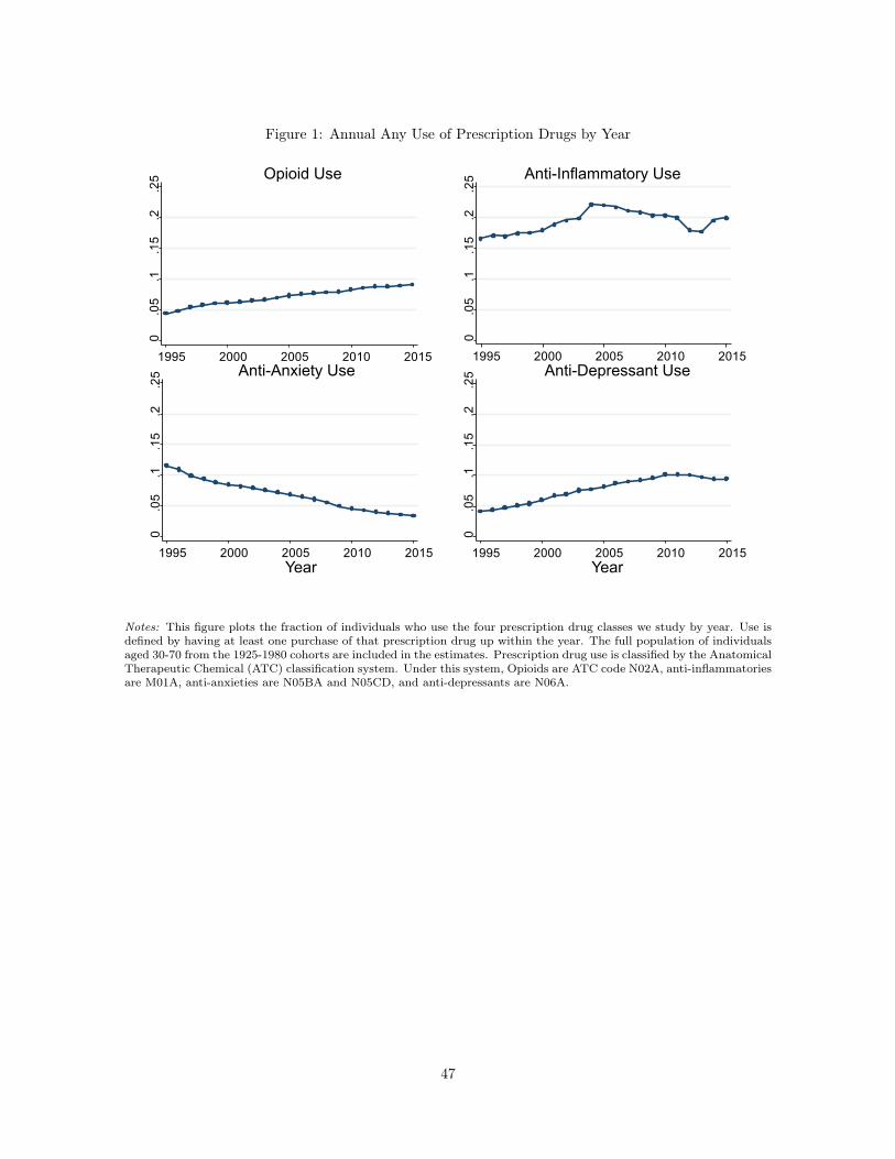
Figure 1: Annual Any Use of Prescription Drugs by Year

Opioid Use Anti-Inflammatory Use

Anti-Anxiety Use

Year

Anti-Depressant Use

Year

0.05

.1.15

.2.25

1995 2000 2005 2010 2015

0.05

.1.15

.2.25

1995 2000 2005 2010 2015

0.05

.1.15

.2.25

1995 2000 2005 2010 2015

0.05

.1.15

.2.25

1995 2000 2005 2010 2015

Notes: This figure plots the fraction of individuals who use the four prescription drug classes we study by year. Use isdefined by having at least one purchase of that prescription drug up within the year. The full population of individualsaged 30-70 from the 1925-1980 cohorts are included in the estimates. Prescription drug use is classified by the AnatomicalTherapeutic Chemical (ATC) classification system. Under this system, Opioids are ATC code N02A, anti-inflammatoriesare M01A, anti-anxieties are N05BA and N05CD, and anti-depressants are N06A.

47

Figure 2: Annual Any Use of Prescription Drugs by Age and Gender

Opioid Use

Men Women

Anti-Inflammatory Use

Anti-Anxiety Use

Age

Anti-Depressant Use

Age

0.1

.2.3

30 40 50 60 70

0.1

.2.3

30 40 50 60 70

0.1

.2.3

30 40 50 60 70

0.1

.2.3

30 40 50 60 70

Notes: This figure plots the fraction of individuals use the four prescription drug classes we study by the age and genderof the individual. The average use of women is plotted with red dots and lines, while the average use of men is plottedusing blue dots and lines. Use is defined by having at least one pick up within the year. The full population of individualsaged 30-70 from the 1925-1980 cohorts for the years 1995-2015 are included in the estimates. See Figure 1 notes for howeach type of drug is classified.

48

Figure 3: Fraction of Individuals that See Pre-Period General Practitioner by Year Since Move

0.2

.4.6

.81

-3 -2 -1 0 1 2 3Year Since Move

See

Pre-

Perio

dG

P

MoversNon-Movers

Notes: Figure 3 plots probability of individuals seeing their pre-period General Practitioner in each year three yearsprior and three years after a move between municipalities for movers (in red dots and lines) and a matched controlsample of non-movers who are assigned a placebo moving year. The control sample is matched exactly on age, gender,education degree, the year, quartiles of each of the four physician prescribing rates, and a quartile of individual’s averagelabor income rank from T � 8 to T � 4. We assign individuals a pre-period General Practitioner (GP) based on the GPindividuals saw the most from T � 3 to T � 1.

49

Figure 4: The Average Change in Physician Prescribing Rate by the Pre-period Physician

Prescribing Rate for Movers and Non-Mover Control Group-.0

4-.0

20

.02

.04

-.04 -.02 0 .02 .04Pre-Period Physician Prescribing Rate

Cha

nge

in P

resc

ribin

gR

ate

a) Opioids

MoversNon-Movers

-.04

-.02

0.0

2.0

4

-.04 -.02 0 .02 .04Pre-Period Physician Prescribing Rate

Cha

nge

in P

resc

ribin

gR

ate

b) Anti-Inflammatories

MoversNon-Movers

-.04

-.02

0.0

2.0

4

-.04 -.02 0 .02 .04Pre-Period Physician Prescribing Rate

Cha

nge

in P

resc

ribin

gR

ate

c) Anti-Anxieties

MoversNon-Movers

-.04

-.02

0.0

2.0

4

-.04 -.02 0 .02 .04Pre-Period Physician Prescribing Rate

Cha

nge

in P

resc

ribin

gR

ate

d) Anti-Depressants

MoversNon-Movers

Notes: This figure plots the average change in physician prescribing rates by the pre-period physician prescribing ratefor movers (red dots and line) and non-movers (blue dots and line). We bin the pre-period physician prescribing ratesinto 20 equal sized bins and plot for the x-axis value, the average pre-period physician prescribing rate within that bin,and for the y-axis value, the average change in prescribing rate for individuals within that bin. The x-axis is in termsof rates, while the y-axis is in terms of change of rates. So in the x-axis a .02 physician prescribing rate of opioidsmeans that 2% of the physician’s patients take opioids. Panel (a) plots the results for opioid physician prescribing rates.Panel (b) plots the results for anti-inflammatory physician prescribing rates. Panel (c) plots the results for anti-anxietyprescribing rates, and finally Panel (d) plots the results for anti-depressant prescribing rates.

50

Figure 5: The Effect of Physician Prescribing Rates on Individual Prescription Drug Use

-3 -2 -1 0 1 2 3

Coe

ffici

ents

Year Since Move

a) Opioids

-.20

.2.4

.6.8

1

Coe

ffici

ents

Year Since Move

b) Anti-Inflammatories

-.20

.2.4

.6.8

1

-3 -2 -1 0 1 2 3

Coe

ffici

ents

Year Since Move

c) Anti-Anxieties

-.20

.2.4

.6.8

1

-3 -2 -1 0 1 2 3

Coe

ffici

ents

Year Since Move

d) Anti-Depressants-.2

0.2

.4.6

.81

-3 -2 -1 0 1 2 3

Notes: This plots the coefficients ✓r(it) from the estimate Equation 3 by the year since the move. The exact interpretationof the coefficients is the change in the relationship between prescription drug use and the relative instrumented changein physician prescribing rates for the year relative to the year prior to the move (T � 1), and for movers relative tonon-movers. However given our assumptions, the coefficients can also be interpreted as the effect of a 1 percentagepoint increase in physician prescribing rates leads to a X percentage point change in drug use. We calculate the relativeinstrumented change in physician prescribing rates in as the difference in the linear fits from Figure 4 of the change in thephysician prescribing rates for a particular pre-period physician prescribing rate between the mover and the non-moversample. Included in the regression are origin by destination by year since event fixed effects (for non-movers the originand destination are the same). This regression is estimated over the years 1995-2015 for individuals aged 30-70. The barsplot the 95% confidence interval for the coefficients. Panel (a) plots the results for opioid physician prescribing rates.Panel (b) plots the results for anti-inflammatory physician prescribing rates. Panel (c) plots the results for anti-anxietyprescribing rates, and finally Panel (d) plots the results for anti-depressant prescribing rates.

51

Figure 6: The Effect of Physician Prescribing Rates on Monthly Individual Prescription Drug Use-.2

-.10

.1.2

-6 -4 -2 0 2 4 6

Coe

ffici

ents

Month Since Move

a) Opioids

-.2-.1

0.1

.2C

oeffi

cien

ts

-6 -4 -2 0 2 4 6

Coe

ffici

ents

Month Since Move

b) Anti-Inflammatories-.2

-.10

.1.2

-6 -4 -2 0 2 4 6

Coe

ffici

ents

Month Since Move

c) Anti-Anxieties

-.2-.1

0.1

.2

-6 -4 -2 0 2 4 6

Coe

ffici

ents

Month Since Move

d) Anti-Depressants

Notes: This figure duplicates Figure 5, but instead of annual prescription drug use as the outcome variable, the outcomevariable is monthly prescription drug use. Additionally, the relationship between drug use and the relative instrumentedchange in physician prescribing rates for movers relative to non-movers is calculated for the 6 months prior to the moveup until 6 months after the move. Thus this figure plots the coefficients ✓r(im) from the estimate Equation 4 by themonth since the move. See Figure 5 for how we calculate the relative instrumented change in physician prescribingrates. The bars plot the 95% confidence interval for the coefficients. Panel (a) plots the results for opioid physicianprescribing rates. Panel (b) plots the results for anti-inflammatory physician prescribing rates. Panel (c) plots the resultsfor anti-anxiety prescribing rates, and finally Panel (d) plots the results for anti-depressant prescribing rates.

52

Figure 7: The Effect of Opioid Physician Prescribing Rates on Labor Income Rank-.4

-.20

.2.4

Coe

ffici

ents

-3 -2 -1 0 1 2 3Year Since Entrance

a) Base Specification

-.4-.2

0.2

.4C

oeffi

cien

ts

-3 -2 -1 0 1 2 3Year Since Entrance

b) Individual Pre-Move Characteristic Controls

-.4-.2

0.2

.4C

oeffi

cien

ts

-3 -2 -1 0 1 2 3Year Since Entrance

c) Individual Pre-Move Characteristic Controls+ Other Physician Prescribing Rates

Notes: This figure replicates Figure 5a, but instead of annual drug use as the outcome variable, the outcome variableis individual’s labor income rank. Specifically, it plots the coefficients ✓Lr(it) in Equation 9 by the year since the move.We can therefore interpret the coefficients as the change in the relationship between labor income rank and the relativeinstrumented change in physician opioid prescribing rates for the year relative to the year prior to the move (T �1), andfor movers relative to non-movers. If our identifying assumptions hold, we can interpret the coefficients as the effect thata 1 percentage point change in physician prescribing rates has on individual’s income in the year since the change. Laborincome is defined as the sum of labor income as well as self employment income. We calculate ranks of labor incomefrom the full population of individuals in Denmark and calculate ranks within year, age, and gender groups. It includesindividuals with zero labor income and is on a scale of 0 to 1. The regression that the coefficients are from is calculatedon the sample of individuals aged 30-70 who move and the non-moving control group from 1995-2013. Panel (a) plotsthe coefficients for a specification with the same set of controls as Figure 5 (a) (municipality origin by destination byyear since move fixed effects). Panel (b) includes controls for individual pre-characteristics by year since the move fixedeffects and whether the individual is treated. Specifically, we include a quadratic in age at the time of the move, gender,and the full interaction of the average labor income rank from T � 8 to T � 4, individual’s years of education, and theirage at the time of the move. Panel (c) includes the same controls as Panel (b), but additionally includes interactionsbetween the relative instrumented change in physician prescribing rates for the other drugs, the year since the move, andan indicator for whether the individual is treated. Therefore, it controls for the effects of the other physician prescribingrates as well.

53

Figure 8: The Effect of Anti-Inflammatory Physician Prescribing Rates on Labor Income Rank-.4

-.20

.2.4

Coe

ffici

ents

-3 -2 -1 0 1 2 3Year Since Entrance

a) Base Specification

-.4-.2

0.2

.4C

oeffi

cien

ts

-3 -2 -1 0 1 2 3Year Since Entrance

b) Individual Pre-Move Characteristic Controls

-.4-.2

0.2

.4C

oeffi

cien

ts

-3 -2 -1 0 1 2 3Year Since Entrance

c) Individual Pre-Move Characteristic Controls+ Other Physician Prescribing Rates

Notes: This figure replicates Figure 7, but instead of the intensity of treatment being the predicted change in opioidprescribing rates, here it is the predicted change in anti-inflammatory prescribing rates. See the notes for Figure 7 fordetails.

54

Figure 9: The Effect of Anti-Anxiety Physician Prescribing Rates on Labor Income Rank-.4

-.20

.2.4

Coe

ffici

ents

-3 -2 -1 0 1 2 3Year Since Entrance

a) Base Specification

-.4-.2

0.2

.4C

oeffi

cien

ts

-3 -2 -1 0 1 2 3Year Since Entrance

b) Individual Pre-Move Characteristic Controls

-.4-.2

0.2

.4C

oeffi

cien

ts

-3 -2 -1 0 1 2 3Year Since Entrance

c) Individual Pre-Move Characteristic Controls+ Other Physician Prescribing Rates

Notes: This figure replicates Figure 7, but instead of the intensity of treatment being the predicted change in opioidprescribing rates, here it is the predicted change in anti-anxiety prescribing rates. See the notes for Figure 7 for details.

55

Figure 10: The Effect of Anti-Depressant Physician Prescribing Rates on Labor Income Rank-.4

-.20

.2.4

Coe

ffici

ents

-3 -2 -1 0 1 2 3Year Since Entrance

a) Base Specification

-.4-.2

0.2

.4C

oeffi

cien

ts

-3 -2 -1 0 1 2 3Year Since Entrance

b) Individual Pre-Move Characteristic Controls

-.4-.2

0.2

.4C

oeffi

cien

ts

-3 -2 -1 0 1 2 3Year Since Entrance

c) Individual Pre-Move Characteristic Controls+ Other Physician Prescribing Rates

Notes: This figure replicates Figure 7, but instead of the intensity of treatment being the predicted change in opioidprescribing rates, here it is the predicted change in anti-depressant prescribing rates. See the notes for Figure 7 fordetails.

56

Figure 11: Heterogeneity in Effect of Physician Opioid Prescribing Rates by Distance of Move-1

.2-1

-.8-.6

-.4-.2

-.7 -.65 -.6 -.55 -.5 -.45 -.4 -.35 -.3Coe

ffici

ento

n Pr

ior P

hysi

cian

Pres

crib

ing

Rat

e

Change in Probability See Same PhysicianBased on Origin & Destination

a) Change in Physician Opioid Prescribing Rates

-1-.8

-.6-.4

-.20

-.7 -.65 -.6 -.55 -.5 -.45 -.4 -.35 -.3Coe

ffici

ento

n P

rior P

hysi

cian

Pre

scrib

ing

Rat

e

Change in Probability See Same PhysicianBased on Origin & Destination

b) Change in Prescription Opioid Use-.4

-.20

.2.4

.6

-.7 -.65 -.6 -.55 -.5 -.45 -.4 -.35 -.3Coe

ffici

ento

n Pr

ior P

hysi

cian

Pres

crib

ing

Rat

e

Change in Probability See Same PhysicianBased on Origin & Destination

c) Change in Labor Income Rank

-.4-.2

0.2

.4.6

-.7 -.65 -.6 -.55 -.5 -.45 -.4 -.35 -.3Coe

ffici

ento

n P

rior P

hysi

cian

Pre

scrib

ing

Rat

e

Change in Probability See Same PhysicianBased on Origin & Destination

d) Change in Labor Income RankWith Other Physician Prescribing Rate Controls

Notes: Panel (a) plots the coefficients of a regression of the change in physician prescribing rate on the pre-periodphysician’s prescribing rate for different binned values of the change in the probability individuals see their same physicianafter their moved, which is based on the origin and destination of their move. Specifically, the change in the probabilityindividuals see their same physician is calculated for all movers like in Figure 3(a), and we take the average difference inthe post-period and the pre-period for all individuals who have the same origin-destination pair (or vice versa). We thenbin these separation rates into 20 equal sized bins. We then estimate a separate coefficient on the pre-period physician’sprescribing rates for each bin in a regression on the change in physician opioid prescribing rates- plotting the coefficientsagainst the mean value of the separation rate. Note that this done only for the moving sample. Panel (b) uses the samex-axis, but we instead plot the coefficients of a regression of individual drug use on the pre-period physician’s prescribingrate interacted with an after indicator and indicators for the different bins of the change in probability that see the samephysician. Panel (c) is the same as Panel (b) except we use labor income rank as the outcome variable. Here we alsoinclude our standard set of controls for individual pre-characteristics (see Figure 7 Panel b) which we estimate separatecoefficients on by bin. Panel (d) replicates (c) but includes controls for the other physician prescribing rates.

57

Appendix Figure 1: Municipality Map of Denmark

Copenhagen

Aarhus

Notes: This figure shows a map of Denmark’s 99 municipalities.

58

Appendix Figure 2: Price of One Pick-up for Prescription Drugs

05

1015

2025

3020

15 D

olla

rs

1995 2000 2005 2010 2015Year

a) Average Price Paid

Change in Subsidy Rules0

2040

6080

100

2015

Dol

lars

1995 2000 2005 2010 2015Year

Opioids Anti-InflammatoriesAnti-Depressants Anti-Anxieties

b) Average Total Cost

Change in Subsidy Rules

Notes: Panel A plots the average subsidized price that individuals paid in 2015 United States dollars for one pick-up ineach year for each of the four types or prescription drugs we study: Opioids, Anti-Inflammatories, Anti-Anxieties, andAnti-Depressants. Panel B plots the non-subsidized cost of the prescription drugs by year for each of the four types ofprescription drugs we study. In 2000, the government changed the subsidy system. Appendix A gives details for the preand post 2000 subsidy systems.

59

Appendix Figure 3: Comparison of United States and Danish Prescription Opioid Drug Use

0

100

200

300

400

500

600

700

800

1995 1997 1999 2001 2003 2005 2007 2009 2011 2013 2015

Mor

phin

e E

quiv

alen

ce M

gs P

er C

apita

Year

USA Denmark

Source: Pain and Policy Studies Group at the University of Wisconsin-Madison, using InternationalNarcotics Control Board and World Health Organization Population data

Notes: This figure uses data aggregated by the Pain and Policy Studies Group at the University of Wisconsin-Madisonusing data from International Narcotics Control Board and World Health Organization Population data. It graphs the percapita consumption of opioids for the United States (blue diamonds) and Denmark (red squares) in terms of MorphineEquivalence Milligrams from 1995-2014. The Pain and Policy Studies Groups developed the Morphine Equivalence(ME) metric using conversion factors from the WHO Collaborating Center for Drugs Statistics Methodology for the 6principal opioids used to treat moderate to severe pain: Fentanyl, Hydromorphone, Methadone, Morphine, Oxycodone,and Pethidine.

60

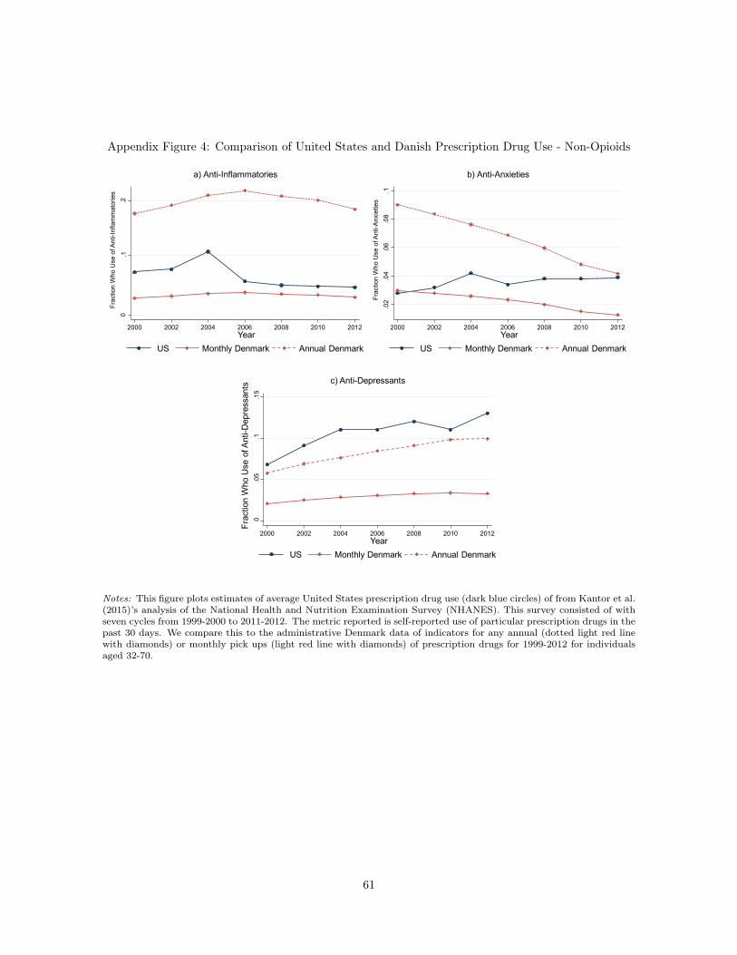
Appendix Figure 4: Comparison of United States and Danish Prescription Drug Use - Non-Opioids

0.2

2000 2002 2004 2006 2008 2010 2012

Frac

tion

Who

Use

of A

nti-I

nfla

mm

ator

ies

.1

a) Anti-Inflammatories

YearUS Monthly Denmark Annual Denmark

.02

.04

.06

.08

.1Fr

actio

nW

hoU

seof

Ant

i-Anx

ietie

s

2000 2002 2004 2006 2008 2010 2012

b) Anti-Anxieties

YearUS Monthly Denmark Annual Denmark

0.0

5.1

.15

Year

Frac

tion

Who

Use

of A

nti-D

epre

ssan

ts c) Anti-Depressants

2000 2002 2004 2006 2008 2010 2012

US Monthly Denmark Annual Denmark

Notes: This figure plots estimates of average United States prescription drug use (dark blue circles) of from Kantor et al.(2015)’s analysis of the National Health and Nutrition Examination Survey (NHANES). This survey consisted of withseven cycles from 1999-2000 to 2011-2012. The metric reported is self-reported use of particular prescription drugs in thepast 30 days. We compare this to the administrative Denmark data of indicators for any annual (dotted light red linewith diamonds) or monthly pick ups (light red line with diamonds) of prescription drugs for 1999-2012 for individualsaged 32-70.

61

Appendix Figure 5: Non-Parametric Effect of a Change in Physician Prescribing Rates on the

Change in Individual Drug Use

-.015

-.01

-.005

0.0

05.0

1.0

15

-.03 -.02 -.01 0 .01 .02 .03

Coe

ffici

ento

n Af

ter*

Mov

er

Predicted Change in Opioid Prescribing Rates

a) Opioids

-.02

-.01

0.0

1.0

2

-.04 -.02 0 .02 .04C

oeffi

cien

ton

Afte

r*M

over

Predicted Change in Anti-Inflammatory Prescribing Rates

b) Anti-Inflammtories

-.015

-.01

-.005

0.0

05.0

1.0

15

-.03 -.02 -.01 0 .01 .02 .03

Coe

ffici

ento

n Af

ter*

Mov

er

Predicted Change in Anti-Anxiety Prescribing Rates

c) Anti-Anxieties

-.015

-.01

-.005

0.0

05.0

1.0

15C

oeffi

cien

ton

Afte

r*M

over

-.03 -.02 -.01 0 .01 .02 .03Predicted Change in Anti-Depressant Prescribing Rates

d) Anti-Depressants

Notes: This figure shows the non-parametric relationship between the change in individual drug use and a change inthe physician prescribing rates. This figure plots the coefficient in a regression of individual prescription drug use onan after indicator interacted with treatment indicator for different values of the predicted relative change in physicianprescribing rates (✓B from Equation 14 in Appendix E). Specifically, we bin the predicted relative change in prescribingrates into 20 equal sized bins. We then create indicators for each bin and interact them with an after indicator and atreatment indicator. We plot the coefficient on each interaction by the mean value of the relative predicted change inphysician prescribing rates. Panel A plots the coefficients for opioid prescription drug use and opioid prescribing rates.Panel B plots the coefficients for anti-inflammatory prescription drug use and anti-inflammatory prescribing rates. PanelC plots the coefficients for anti-anxiety prescription drug use and anti-anxiety prescribing rates, and Panel D plots thecoefficients for anti-depressant prescription drug use an anti-depressant prescribing rates.

62

Appendix Figure 6: Heterogeneity in the Effect of Physician Anti-Inflammatory Prescribing Rates by

Distance of Move-1

.2-1

-.8-.6

-.4-.2

-.7 -.65 -.6 -.55 -.5 -.45 -.4 -.35 -.3Coe

ffici

ento

n Pr

ior P

hysi

cian

Pres

crib

ing

Rat

e

Change in Probability See Same PhysicianBased on Origin & Destination

a) Change in Physician Anti-Inflammatory Prescribing Rates

-1-.8

-.6-.4

-.20

-.7 -.65 -.6 -.55 -.5 -.45 -.4 -.35 -.3Coe

ffici

ento

n P

rior P

hysi

cian

Pre

scrib

ing

Rat

e

Change in Probability See Same PhysicianBased on Origin & Destination

b) Change in Prescription Anti-Inflammatory Use

-.4-.2

0.2

.4.6

-.7 -.65 -.6 -.55 -.5 -.45 -.4 -.35 -.3Coe

ffici

ento

n Pr

ior P

hysi

cian

Pres

crib

ing

Rat

e

Change in Probability See Same PhysicianBased on Origin & Destination

c) Change in Labor Income Rank-.4

-.20

.2.4

.6

-.7 -.65 -.6 -.55 -.5 -.45 -.4 -.35 -.3Coe

ffici

ento

n P

rior P

hysi

cian

Pre

scrib

ing

Rat

e

Change in Probability See Same PhysicianBased on Origin & Destination

d) Change in Labor Income RankWith Other Physician Prescribing Rate Controls

Notes: This figure shows heterogeneity in the effect of physician anti-inflammatory rates by the distance of the move- measured by the average separation rate with pre-move physicians. It looks at the effects of this heterogeneity on:the relationship between the change in physician prescribing rates and pre-move physician prescribing rates (Panel A),the relationship between the change in individual drug use and pre-move physician prescribing rates (Panel B), therelationship between the change in labor income rank and the pre-move physician’s prescribing rates (Panel C and D).It replicates Figure 11, except for instead of opioid drug use and opioid prescribing rates, it looks at anti-inflammatoryuse and anti-inflammatory prescribing rates. See Figure 11 notes for additional details.

63

Appendix Figure 7: Heterogeneity in the Effect of Physician Anti-Anxiety Prescribing Rates by the

Distance of Move

-1.2

-1-.8

-.6-.4

-.2

-.7 -.65 -.6 -.55 -.5 -.45 -.4 -.35 -.3Coe

ffici

ento

n Pr

ior P

hysi

cian

Pres

crib

ing

Rat

e

Change in Probability See Same PhysicianBased on Origin & Destination

a) Change in Physician Anti-Anxiety Prescribing Rates

-1-.8

-.6-.4

-.20

-.7 -.65 -.6 -.55 -.5 -.45 -.4 -.35 -.3Coe

ffici

ento

n P

rior P

hysi

cian

Pre

scrib

ing

Rat

eChange in Probability See Same Physician

Based on Origin & Destination

b) Change in Prescription Anti-Anxiety Use

-.4-.2

0.2

.4.6

-.7 -.65 -.6 -.55 -.5 -.45 -.4 -.35 -.3Coe

ffici

ento

n Pr

ior P

hysi

cian

Pres

crib

ing

Rat

e

Change in Probability See Same PhysicianBased on Origin & Destination

c) Change in Labor Income Rank

-.04

-.02

0.0

2.0

4

-.04 -.02 0 .02 .04Pre-Period Physician Prescribing Rate

Cha

nge

in P

resc

ribin

gR

ate

d) Anti-Depressants

MoversNon-Movers

Notes: This figure shows heterogeneity in the effect of physician anti-anxiety rates by the distance of the move - measuredby the average separation rate with pre-move physicians. It looks at the effects of this heterogeneity on: the relationshipbetween the change in physician prescribing rates and pre-move physician prescribing rates (Panel A), the relationshipbetween the change in individual drug use and pre-move physician prescribing rates (Panel B), the relationship betweenthe change in labor income rank and the pre-move physician’s prescribing rates (Panel C and D). It replicates Figure 11,except for instead of opioid drug use and opioid prescribing rates, it looks at anti-anxiety use and anti-anxiety prescribingrates. See Figure 11 notes for additional details.

64

Appendix Figure 8: Heterogeneity in the Effect of Physician Anti-Depressant Prescribing Rates by

the Distance of Move

-1.2

-1-.8

-.6-.4

-.2

-.7 -.65 -.6 -.55 -.5 -.45 -.4 -.35 -.3Coe

ffici

ento

n Pr

ior P

hysi

cian

Pres

crib

ing

Rat

e

Change in Probability See Same PhysicianBased on Origin & Destination

a) Change in Physician Anti-Depressant Prescribing Rates

-1-.8

-.6-.4

-.20

-.7 -.65 -.6 -.55 -.5 -.45 -.4 -.35 -.3Coe

ffici

ento

n P

rior P

hysi

cian

Pre

scrib

ing

Rat

eChange in Probability See Same Physician

Based on Origin & Destination

b) Change in Prescription Anti-Depressant Use

-.4-.2

0.2

.4.6

-.7 -.65 -.6 -.55 -.5 -.45 -.4 -.35 -.3Coe

ffici

ento

n Pr

ior P

hysi

cian

Pres

crib

ing

Rat

e

Change in Probability See Same PhysicianBased on Origin & Destination

c) Change in Labor Income Rank

-.4-.2

0.2

.4.6

-.7 -.65 -.6 -.55 -.5 -.45 -.4 -.35 -.3Coe

ffici

ento

n P

rior P

hysi

cian

Pre

scrib

ing

Rat

e

Change in Probability See Same PhysicianBased on Origin & Destination

d) Change in Labor Income RankWith Other Physician Prescribing Rate Controls

Notes: This figure shows heterogeneity in the effect of physician anti-depressant rates by the distance of the move -measured by the average separation rate with pre-move physicians. It looks at the effects of this heterogeneity on:the relationship between the change in physician prescribing rates and pre-move physician prescribing rates (Panel A),the relationship between the change in individual drug use and pre-move physician prescribing rates (Panel B), therelationship between the change in labor income rank and the pre-move physician’s prescribing rates (Panel C and D).It replicates Figure 11, except for instead of opioid drug use and opioid prescribing rates, it looks at anti-depressant useand anti-depressant prescribing rates. See Figure 11 notes for additional details.

65

Opioids Anti-Inflammatories

Anti-Anxieties

Anti-Depressants

(1) (2) (3) (4)Standard Deviation of Physician Effects

Raw Physician Averages 0.023 0.036 0.029 0.021

Estimated Physician Effects 0.018 0.029 0.024 0.017

Intstrumented Change in 0.009 0.015 0.012 0.010Physician Prescription Rates

Mean Prescription Rate 0.070 0.193 0.075 0.078

Table 1: Standard Deviation of Physician Prescription Rates

Notes: This table presents the standard deviation of physician prescribing rates, for each type of drug. Prescribing rates are the fraction of patients who pick up a prescription for the drug within a year and can range from 0 (none of the physician's patients take the drug) to 1 (all of the physician's patients take the drug). Individuals are assigned to primary care physicians in a given year based on the general practitioner they see the most in the year before, the year of, and the year after. All individuals aged 30-70 from the cohorts 1925-1980 and from the years 1995-2015 are used to calculate the prescribing rates. Physicians with fewer than 1000 patients are excluded. Row 1 reports the standard deviation of raw physician averages. Row 2 reports the standard deviations of the physician effects we estimate from Equation 1, which takes out variation from the patients age, education, gender, and the year. Row 3 reports the standard deviation of the actual treatment we use, which is the instrumented relative change in physician prescribing rates based on the individual's pre-move physician. The last row reports the fraction of annual usage for individuals aged 30-70, cohorts 1925-1980, and the years 1995-2015. Column (1) reports the standard deviation for opioid prescribing rates, column (2) reports the standard deviations for anti-inflammatory (NSAIDs) prescribing rates, column (3) reports the standard deviations for anti-anxiety (benzodiazapine) prescribing rates, and column (4) reports the standard deviations for anti-depressant prescribing rates.

OpioidsAnti-

InflammatoriesAnti-

AnxietiesAnti-

Depressants(1) (2) (3) (4)

After * Mover * 0.448*** 0.585*** 0.359*** 0.467*** Predicted ! in Physician (0.0360) (0.0338) (0.0273) (0.0401) Prescribing Rates

N 15,324,329 15,324,329 15,324,329 15,324,329

* p<0.05 ** p<0.01 *** p<0.001

Table 2: The Effects of Physician Prescribing Rates on Prescription Drugs

Prescription Drug Use

Notes: This table presents the estimated coefficients from Equation (5) in the paper: a regression of individual prescription drug use (an indicator variable) on the interaction of an indicator for after the move, whether the individual is a mover, and the relative predicted change in physician prescribing rates based on the pre-period physician's prescribing rate. Also in the regression includes the full set of pairs of interactions between those three variables, as well as origin by desitination by an indicator for after fixed effects. The regression includes individuals who move across municipalities at time T=0, as well as a matched set of individuals who do not move who are matched by year, age, gender, education, quartiles of prior physician prescribing rates, and a quartile for the individual's average income rank from T-8 to T-4 . Observations up to three years after the move and three years prior to the move are included in the regression, while the year of the move is not. Individuals who are aged 30-70 and from the years 1995-2015 are included. The relative predicted change in physician prescribing rates is the difference for the mover and non-mover sample of the linear prediction from a regression of change in physician prescribing rates from after the "move" from before the "move" on their prior physician prescribing rates. Column (1) presents the results when the relative predicted change in prescribing rates is for opioids, and the outcome measure is opioid prescription drug use. Column (2) presente the results when the prescribing rate and the outcome measure is for anti-inflammatories. Column (3) presents the results when the prescribing rate and the outcome measure is for anti-anxieties, and Column (4) presents the results for when the outcome measure is for anti-depressants. Standard errors are reported before the coefficients and calculated by clustering at the individual level. Given that the dependent variable is an indicator, and the treatment variable is in terms of a rate, the interpretation of coefficient in column (1) is the effect of a 1 percentage point increase in the relative predicted change in physician prescribing rates leads to a .45 percentage point increase in opioid prescription drug use for movers relative to non-movers, after the move compared to before the move.

X: Old Female Educated Blue-Collar(1) (2) (3) (4)

A. OpioidsAfter * ! * Mover 0.342*** 0.353*** 0.533*** 0.279***

(0.0464) (0.0464) (0.0428) (0.0474)

After * ! * Mover * X 0.227*** 0.211** -0.228*** 0.249***(0.0663) (0.0666) (0.0676) (0.0692)

B. Anti-InflammatoriesAfter * ! * Mover 0.548*** 0.549*** 0.652*** 0.554***

(0.0458) (0.0460) (0.0419) (0.0484)

After * ! * Mover * X 0.0695 0.0968 -0.168* 0.0931(0.0647) (0.0649) (0.0658) (0.0716)

C. Anti-AnxietiesAfter * ! * Mover 0.305*** 0.318*** 0.384*** 0.274***

(0.0345) (0.0350) (0.0326) (0.0350)

After * ! * Mover * X 0.132** 0.0987* -0.0734 0.125*(0.0498) (0.0498) (0.0506) (0.0524)

D. Anti-DepressantsAfter * ! * Mover 0.471*** 0.386*** 0.520*** 0.404***

(0.0505) (0.0514) (0.0475) (0.0517)

After * ! * Mover * X 0.0141 0.154* -0.134 0.161*(0.0727) (0.0725) (0.0736) (0.0769)

N 15,324,329 15,324,329 15,324,329 12407329

* p<0.05 ** p<0.01 *** p<0.001

Prescription Drug Use

Table 3: Heterogeneity of Treatment Effects on Prescription Drugs

Notes: This table presents the estimated coefficients from Equation 8 in the paper: a regression of prescription drug use on the full interaction between an indicator for after the move, whether the individual is a mover, the predicted relative change in the physician prescribing rate, and an indicator for characteristic X. We report the coefficients of the effect of physician prescribing rates for those with out the characteristic (e.g. the first row of Panel A), and the difference in the effect for those with the characteristic versus those without the characteristic (e.g. the second row of Panel A). Panel A reports the reults for opioid prescribing rates and opioid prescription drug use, while Panel B is for anti-inflammatory prescribing rates and anti-inflammatory prescription drug use, Panel C is for anti-anxiety prescribing rates and anti-anxiety prescription drug use, and Panel D is for anti-depressant prescribing rates and anti-depressant prescription drug use. Column (1) presents the results when the indicator is for individual being older than 42 at the time of the move, while Column (2) is for an indicator of female, Column (3) for an indicator of having more than 14 years of education, and column 4 for individual being in a blue collar occupation in T-4. It includes the sample sample as Table 2.

(1) (2) (3)A. Opioids

After * ! * Mover -0.113*** -0.117*** -0.123*(0.0366) (0.0323) (0.0467)

B. Anti-InflammatoriesAfter * ! * Mover 0.0334 -0.0354 -0.00156

(0.0225) (0.0199) (0.0223)

C. Anti-AnxietiesAfter * ! * Mover -0.0878** -0.0346 0.0546

(0.0283) (0.0248) (0.0345)

D. Anti-DepressantsAfter * ! * Mover -0.145*** -0.110*** -0.0774*

(0.0361) (0.0320) (0.0382)

ControlsInd Pre-Chars x Yr Since Event x Moved x xOther Prescribing Rates x

N 15324329 15171445 15171445

* p<0.05 ** p<0.01 *** p<0.001

Table 4: The Effects of Physician Prescribing Rates on Labor Income Rank

Labor Income Rank

Notes: This table presents the estimated coefficients from a regression of labor income rank on the interaction of an indicator for after the move, whether the individual is a mover, and the relative predicted change in physician prescribing rates based on the pre-period physician's prescribing rate. Also in the regression includes the full set of pairs of interactions between those three variables, as well as origin by desitination by an indicator for after fixed effects. We measure labor income as taxable labor and self-employed earnings. We convert labor income into percentile ranks within an individual's year of birth, the year, and their gender using the full sample of the Danish population (not just the movers and non-mover control sample). It is on a scale from 0 (lowest income) to 1 (highest income). Column (1) replicates the specifications from Table 2, substituting labor income rank as the left-hand side variable instead of prescription drug use. Column (2) additionally includes control for individual pre-characteristics that are fully interacted with an indicator for after and an indicator for being a mover. The pre-characteristics include a quadratic in age at the time of move, an indicator for female, and the full interaction of average labor income rank over T-8 to T-4, years of education, and age. Column (3) additionally includes the full interactions of the other prescription rates and indicators for after and being a mover. Thus Column (3) represents coefficients from all the same regression, whereas Column (1)-(2) each report coefficients from four different regressions.

Physician Prescribing Rates:Opioids Anti-

InflammatoriesAnti-

Anxieities(1) (2) (3)

A. Correlation of Physician AveragesAnti-Inflammatories 0.403Anti-Anxieities 0.553 0.230Anti-Depressants 0.455 0.304 0.362

B. Correlation of Relative Predicted ChangeAnti-Inflammatories 0.428Anti-Anxieities 0.476 0.307Anti-Depressants 0.565 0.235 0.382

Table 5: Correlation Between Physician Prescribing Rates

Notes: This table presents the correlations between physician prescription rates of different drugs (Panel A) and the correlation between the relative predicted change in physician prescribing rates. Both are weighted by the estimating sample we us in Table 2. Physician prescribing rates are calculated by first taking out effects from immutable individual characteristics, specifically: of age, gender, education and the year. The relative predicted change is estimated as explained in the Notes of Table 2, using the difference in the predicted change in prescribing rates based on the pre-move physician for movers and non-movers.

Labor Income Rank

LFP Log Labor Income

Labor Inc. Rank Pos. LFP

Any Sick Pay Sick Pay > 4 weeks

DI Receipt

(1) (2) (3) (4) (5) (6) (7)A. Opioids

After * ! * Mover -0.123* -0.196** -2.316** -0.0651 0.0481 0.146 0.0109(0.0467) (0.0699) (0.844) (0.0476) (0.0808) (0.0824) (0.0470)

B. Anti-InflammatoriesAfter * ! * Mover -0.00156 -0.0108 -0.182 0.0161 -0.0413 0.0200 0.0405

(0.0223) (0.0330) (0.399) (0.0225) (0.0384) (0.0388) (0.0220)

C. Anti-AnxietiesAfter * ! * Mover 0.0546 0.0859 1.058 0.0383 -0.0152 -0.0342 -0.0532

(0.0345) (0.0512) (0.619) (0.0350) (0.0585) (0.0596) (0.0339)

D. Anti-DepressantsAfter * ! * Mover -0.0774* -0.0312 -0.773 -0.0615 -0.0487 -0.111 0.0512

(0.0382) (0.0573) (0.691) (0.0391) (0.0660) (0.0680) (0.0399)

N 15171445 15171445 15171445 12469064 8964761 8587148 13750107

* p<0.05 ** p<0.01 *** p<0.001

Table 6: The Effects of Physician Prescribing Rates on Other Labor Outcomes with Full Controls

Notes: Column (1) of this table replicates Column (3) of Table (4). The other columns use the same set of controls but change the outcome variables. The outcome variable for Column (2) is labor force participation which is an indicator variable for having positive labor income. For Column (3), log labor income is defined as ln (Labor Income +1), where labor income is first put into 2015 Danish Kroner (6.5 Dkr~1$) using the Danish CPI. Column (4) replicates column (1) but only includes individuals with positive labor income. Column (5)'s outcome measure is an indicator for any sick pay which is an indicator for whether their employer paid them any sick pay within the year. It is defined only for private sector employees. The outcome variable in Column (6) is an indicator for taking sick pay longer than four weeks, which is identified by whether the municipality paid sick pay for private section employees. Because it also includes payments for maternity leave, we set it equal to missing for women who had a baby within the year or the year previous. Column (7) reports the results for when the outcome variable is Disability Insurance receipt which is defined for indviduals less than 65 and is also an indicator variable.

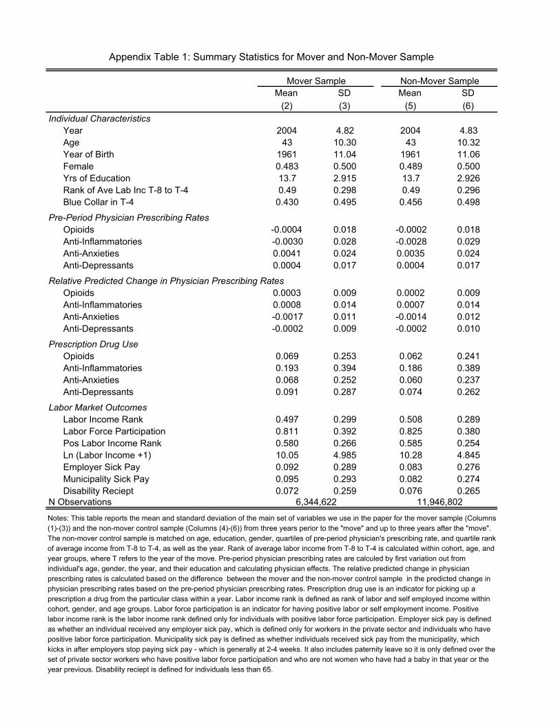
Mean SD Mean SD(2) (3) (5) (6)

Individual CharacteristicsYear 2004 4.82 2004 4.83Age 43 10.30 43 10.32Year of Birth 1961 11.04 1961 11.06Female 0.483 0.500 0.489 0.500Yrs of Education 13.7 2.915 13.7 2.926Rank of Ave Lab Inc T-8 to T-4 0.49 0.298 0.49 0.296Blue Collar in T-4 0.430 0.495 0.456 0.498

Pre-Period Physician Prescribing RatesOpioids -0.0004 0.018 -0.0002 0.018Anti-Inflammatories -0.0030 0.028 -0.0028 0.029Anti-Anxieties 0.0041 0.024 0.0035 0.024Anti-Depressants 0.0004 0.017 0.0004 0.017

Relative Predicted Change in Physician Prescribing RatesOpioids 0.0003 0.009 0.0002 0.009Anti-Inflammatories 0.0008 0.014 0.0007 0.014Anti-Anxieties -0.0017 0.011 -0.0014 0.012Anti-Depressants -0.0002 0.009 -0.0002 0.010

Prescription Drug UseOpioids 0.069 0.253 0.062 0.241Anti-Inflammatories 0.193 0.394 0.186 0.389Anti-Anxieties 0.068 0.252 0.060 0.237Anti-Depressants 0.091 0.287 0.074 0.262

Labor Market OutcomesLabor Income Rank 0.497 0.299 0.508 0.289Labor Force Participation 0.811 0.392 0.825 0.380Pos Labor Income Rank 0.580 0.266 0.585 0.254Ln (Labor Income +1) 10.05 4.985 10.28 4.845Employer Sick Pay 0.092 0.289 0.083 0.276Municipality Sick Pay 0.095 0.293 0.082 0.274Disability Reciept 0.072 0.259 0.076 0.265

N Observations

Mover Sample Non-Mover Sample

Appendix Table 1: Summary Statistics for Mover and Non-Mover Sample

Notes: This table reports the mean and standard deviation of the main set of variables we use in the paper for the mover sample (Columns (1)-(3)) and the non-mover control sample (Columns (4)-(6)) from three years perior to the "move" and up to three years after the "move". The non-mover control sample is matched on age, education, gender, quartiles of pre-period physician's prescribing rate, and quartile rank of average income from T-8 to T-4, as well as the year. Rank of average labor income from T-8 to T-4 is calculated within cohort, age, and year groups, where T refers to the year of the move. Pre-period physician prescribing rates are calculed by first variation out from individual's age, gender, the year, and their education and calculating physician effects. The relative predicted change in physician prescribing rates is calculated based on the difference between the mover and the non-mover control sample in the predicted change in physician prescribing rates based on the pre-period physician prescribing rates. Prescription drug use is an indicator for picking up a prescription a drug from the particular class within a year. Labor income rank is defined as rank of labor and self employed income within cohort, gender, and age groups. Labor force participation is an indicator for having positive labor or self employment income. Positive labor income rank is the labor income rank defined only for individuals with positive labor force participation. Employer sick pay is defined as whether an individual received any employer sick pay, which is defined only for workers in the private sector and individuals who have positive labor force participation. Municipality sick pay is defined as whether individuals received sick pay from the municipality, which kicks in after employers stop paying sick pay - which is generally at 2-4 weeks. It also includes paternity leave so it is only defined over the set of private sector workers who have positive labor force participation and who are not women who have had a baby in that year or the year previous. Disability reciept is defined for individuals less than 65.

6,344,622 11,946,802

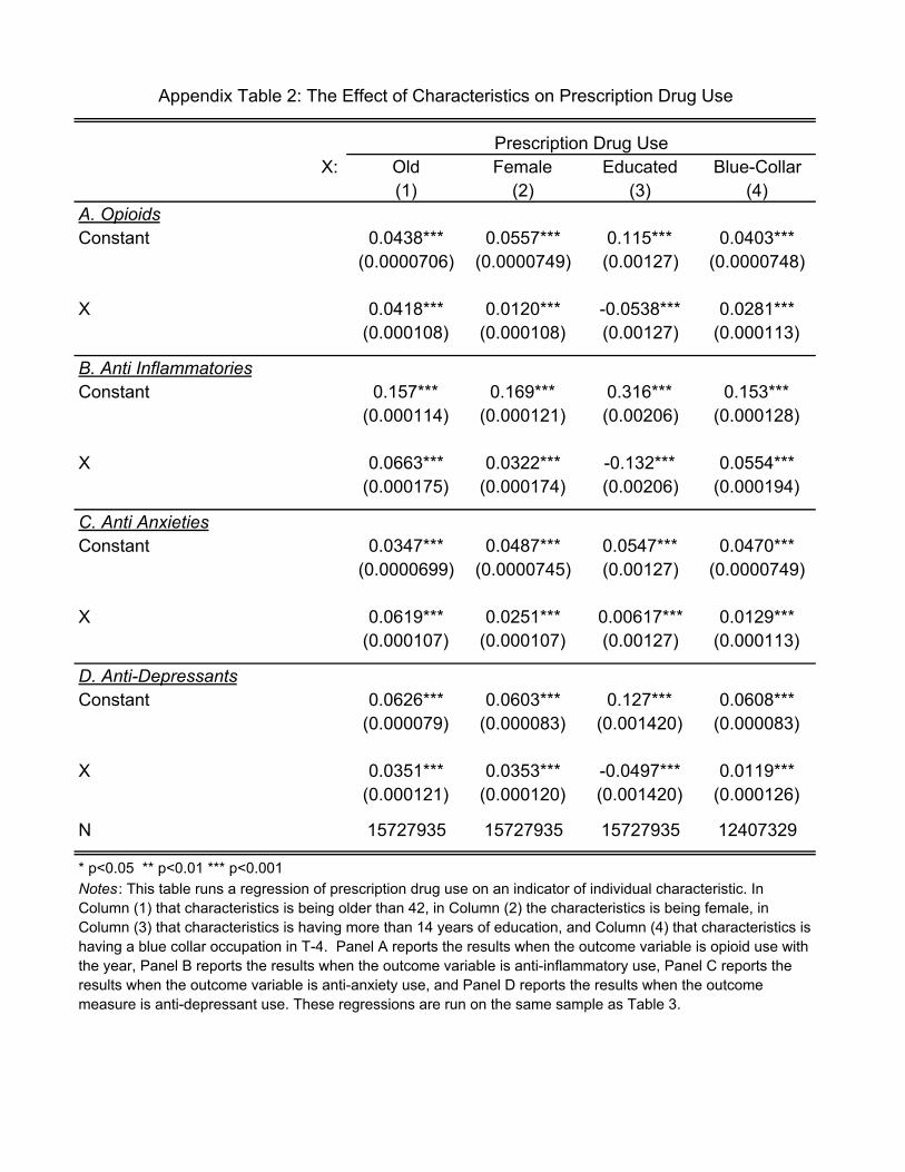
X: Old Female Educated Blue-Collar(1) (2) (3) (4)

A. OpioidsConstant 0.0438*** 0.0557*** 0.115*** 0.0403***

(0.0000706) (0.0000749) (0.00127) (0.0000748)

X 0.0418*** 0.0120*** -0.0538*** 0.0281***(0.000108) (0.000108) (0.00127) (0.000113)

B. Anti InflammatoriesConstant 0.157*** 0.169*** 0.316*** 0.153***

(0.000114) (0.000121) (0.00206) (0.000128)

X 0.0663*** 0.0322*** -0.132*** 0.0554***(0.000175) (0.000174) (0.00206) (0.000194)

C. Anti AnxietiesConstant 0.0347*** 0.0487*** 0.0547*** 0.0470***

(0.0000699) (0.0000745) (0.00127) (0.0000749)

X 0.0619*** 0.0251*** 0.00617*** 0.0129***(0.000107) (0.000107) (0.00127) (0.000113)

D. Anti-DepressantsConstant 0.0626*** 0.0603*** 0.127*** 0.0608***

(0.000079) (0.000083) (0.001420) (0.000083)

X 0.0351*** 0.0353*** -0.0497*** 0.0119***(0.000121) (0.000120) (0.001420) (0.000126)

N 15727935 15727935 15727935 12407329

* p<0.05 ** p<0.01 *** p<0.001

Appendix Table 2: The Effect of Characteristics on Prescription Drug Use

Prescription Drug Use

Notes : This table runs a regression of prescription drug use on an indicator of individual characteristic. In Column (1) that characteristics is being older than 42, in Column (2) the characteristics is being female, in Column (3) that characteristics is having more than 14 years of education, and Column (4) that characteristics is having a blue collar occupation in T-4. Panel A reports the results when the outcome variable is opioid use with the year, Panel B reports the results when the outcome variable is anti-inflammatory use, Panel C reports the results when the outcome variable is anti-anxiety use, and Panel D reports the results when the outcome measure is anti-depressant use. These regressions are run on the same sample as Table 3.

OpioidsAnti-

InflammatoriesAnti-

AnxietiesAnti-

Depressants(1) (2) (3) (4)

After * Mover * 0.609*** 0.704*** 0.515*** 0.460*** Predicted ! in Physician (0.0513) (0.0382) (0.0478) (0.0382) Prescribing Rates

N 15,324,329 15,324,329 15,324,329 15,324,329

* p<0.05 ** p<0.01 *** p<0.001

Appendix Table 3: The Effects of Physician Prescribing Rates on Prescription Drugs Horse Race

Prescription Drug Use

Notes: This table replicates Table 2 but includes the relative predicated change in prescribing rates for all drugs, so that the coefficients from four columns come from the same regression.

Labor Income

Rank

LFP Log Labor

Income

Labor Inc.

Rank Pos. LFP

Sick Pay

Employer

Sick Pay

Municipality

DI Receipt

(1) (2) (3) (4) (5) (6) (7)

A. OpioidsAfter * ! * Mover -0.117*** -0.145** -1.923** -0.0732 -0.0152 0.0726 0.0176

(0.0323) (0.0490) (0.591) (0.0392) (0.0563) (0.0577) (0.0335)

B. Anti InflammatoriesAfter * ! * Mover -0.0354 -0.0454 -0.667 -0.00194 -0.0425 0.0238 0.0422*

(0.0199) (0.0295) (0.356) (0.0238) (0.0340) (0.0345) (0.0197)

C. Anti AnxietiesAfter * ! * Mover -0.0346 -0.0249 -0.416 -0.00791 -0.0288 0.00491 -0.0118

(0.0248) (0.0371) (0.447) (0.0298) (0.0424) (0.0432) (0.0246)

D. Anti-DepressantsAfter * ! * Mover -0.110*** -0.0858 -1.429* -0.0902* -0.0576 -0.0526 0.0517

(0.0320) (0.0480) (0.579) (0.0386) (0.0548) (0.0566) (0.0337)

N 15171445 15171445 15171445 12469064 8964761 8587148 13750107

* p<0.05 ** p<0.01 *** p<0.001

Appendix Table 4: The Effects of Physician Prescribing Rates on Other Labor Outcomes - Not Horse Race

Notes : This table replicates Table 6, except instead of including the relative change of physician prescribing rates all together in the same regression, we

estimate the coefficients in separate regressions, one for each panel within a column.

X: Old Female Educated Blue-Collar(1) (2) (3) (4)

A. OpioidsAfter * ! * Mover -0.106 -0.166** -0.189*** -0.191**

(0.0613) (0.0608) (0.0555) (0.0660)

After * ! * Mover * X -0.0186 0.0815 0.101 0.0993(0.0862) (0.0866) (0.0882) (0.0960)

B. Anti-InflammatoriesAfter * ! * Mover 0.0224 0.00120 -0.0364 0.0460

(0.0293) (0.0293) (0.0265) (0.0312)

After * ! * Mover * X -0.0397 0.00335 0.0663 -0.0719(0.0411) (0.0414) (0.0419) (0.0459)

C. Anti-AnxietiesAfter * ! * Mover 0.00841 0.0831 0.153*** 0.0719

(0.0449) (0.0449) (0.0415) (0.0478)

After * ! * Mover * X 0.141* -0.0507 -0.155* -0.0210(0.0637) (0.0637) (0.0649) (0.0711)

D. Anti-DepressantsAfter * ! * Mover -0.143** -0.0544 -0.0617 -0.0983

(0.0494) (0.0505) (0.0463) (0.0544)

After * ! * Mover * X 0.106 -0.0519 -0.0661 0.0521(0.0708) (0.0710) (0.0719) (0.0804)

N 15171445 15171445 15171445 12096004

* p<0.05 ** p<0.01 *** p<0.001

Appendix Table 5: Heterogeneity of the Effects on Labor Income Rank - Horse Race

Labor Income Rank

Notes: This table replicates Table 3, however, labor income rank is the outcome variable, and we include all of the physician prescribing rates interacted fully with an indicator for after, the predicted relative change in prescribing rates, and indicator for mover and an indicator for the characteristics. Therefore now each column reports coefficients from the same regression. We also include the controls from Table 4 Column (3) also interacted with the characteristic. We measure labor income as taxable labor and self-employed earnings. We convert labor income into percentile ranks within an individual's year of birth, the year, and their gender using the full sample of the Danish population (not just the movers and non-mover control sample). It is on a scale from 0 (lowest income) to 1 (highest income). Appendix Table 5 reports the coefficients when we separately control for each prescribing rate in separate regressions.

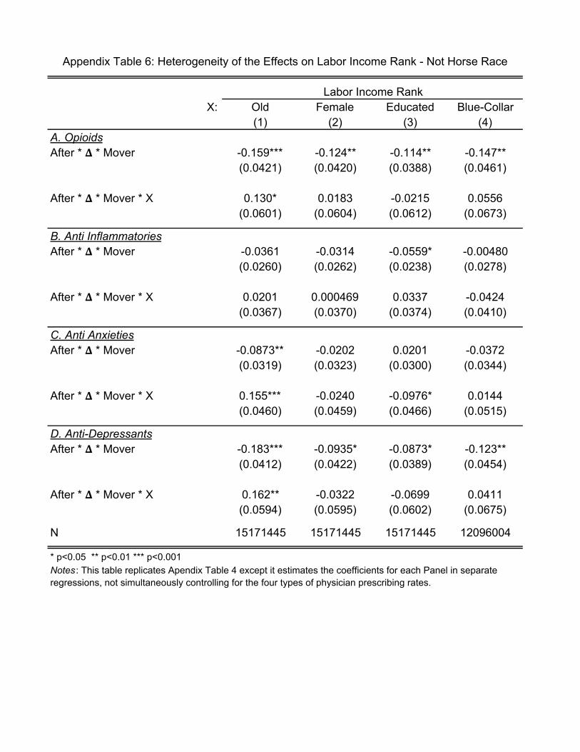
X: Old Female Educated Blue-Collar(1) (2) (3) (4)

A. OpioidsAfter * ! * Mover -0.159*** -0.124** -0.114** -0.147**

(0.0421) (0.0420) (0.0388) (0.0461)

After * ! * Mover * X 0.130* 0.0183 -0.0215 0.0556(0.0601) (0.0604) (0.0612) (0.0673)

B. Anti InflammatoriesAfter * ! * Mover -0.0361 -0.0314 -0.0559* -0.00480

(0.0260) (0.0262) (0.0238) (0.0278)

After * ! * Mover * X 0.0201 0.000469 0.0337 -0.0424(0.0367) (0.0370) (0.0374) (0.0410)

C. Anti AnxietiesAfter * ! * Mover -0.0873** -0.0202 0.0201 -0.0372

(0.0319) (0.0323) (0.0300) (0.0344)

After * ! * Mover * X 0.155*** -0.0240 -0.0976* 0.0144(0.0460) (0.0459) (0.0466) (0.0515)

D. Anti-DepressantsAfter * ! * Mover -0.183*** -0.0935* -0.0873* -0.123**

(0.0412) (0.0422) (0.0389) (0.0454)

After * ! * Mover * X 0.162** -0.0322 -0.0699 0.0411(0.0594) (0.0595) (0.0602) (0.0675)

N 15171445 15171445 15171445 12096004

* p<0.05 ** p<0.01 *** p<0.001

Appendix Table 6: Heterogeneity of the Effects on Labor Income Rank - Not Horse Race

Labor Income Rank

Notes : This table replicates Apendix Table 4 except it estimates the coefficients for each Panel in separate regressions, not simultaneously controlling for the four types of physician prescribing rates.