Embed Size (px)
Citation preview

THE ECONOMIST DIWAN
Issue 1 | Spring 2017
2 About the Journal
3 Editor’s Note
4 Message from the Dean
5 Message from the Head of the Department of Economics
6 Investigating the Asymmetric Impact of Unemployment on Property Crime
Pallavi Mandar Bichu
24 Quantifying the Oil Price Plunge
Husain Rangwalla
41 A Cross Country Panel Study of the Relationship between Urbanization and
Suicide in Japan and Korea Jason Torion

2
ABOUT THE JOURNAL
The Economist Diwan is be a student-run academic journal that provides an opportunity
to publish the best research done in economics and related fields at the American University of
Sharjah (AUS). Starting its first publication in Spring 2017, this journal operates under the
AUS Department of Economics in the School of Business Administration (SBA). Our aim is
to publish research carried out by students in the American University of Sharjah (AUS),
exchange students at AUS and potentially extending our reach to publishing undergraduate
research from other universities in the region as well.
Through this journal, the AUS Department of Economics intends to promote the diverse
application of economics related concepts amongst its current and prospective students. For
any other inquiries or if you wish to contribute, feel free to contact us via

3
EDITOR’S NOTE
The Economist Diwan is a journal meant for students to have an overview of the
research fellow students have conducted in Economics. One of the aims of this student-run
journal is for other undergraduates to understand the various applications of the theories and
empirical methods pursued in Economics to explore and gain a different perspective of topics
beyond the customary demand and supply applications in the classroom. Economics is a social
science, and a rather unique one at that. Using a few concepts from many fields of study such
as Physics, Mathematics, Business and applying a behavioral context to qualitative data,
economists analyze datasets and results in a different perspective from fellow peers in other
streams of study.
It has become a common phenomenon for sociologists, economists and
mathematicians, for example, to confront a research topic together to maximize analysis and
results. The quality of research publications has certainly improved over the past decades along
with the refinement of economics as a field of study. Many political and behavioral theories
are in existence today thanks to the empirical methods economics has to offer.
What we hope is for this journal to become, in the future, a gateway and foundation for
aspiring and self-motivated young economists to be able to independently conduct research,
even at the undergraduate stage and experience its publication. We envision this student-run
journal to be one that even students outside AUS will proudly contribute to. We want to plant
seeds that will hopefully bloom into what is a student research community in the UAE.
Mehr Patni
Chief Editor & Co-Founder
BA, Economics
Jason Paulo Torion
Chief Editor & Co-Founder
BSBA, Economics
4
MESSAGE FROM THE DEAN
Teaching and research are the pillars of academia. Professors transfer knowledge to their
students and simultaneously conduct analytical studies that help expand the boundaries of their
respective disciplines. The results of this research find its way back to the students and enrich
classroom discussions and directed studies. As students go through their degree programs and
evolve from memorizing to understanding to applying and finally to synthesizing knowledge,
they increasingly become part of this academic cycle. The brightest of them transform from
being mere consumers to seekers and creators of knowledge, using an array of analytical tools.
Examples of this student-based knowledge creation that touch on a variety of exploratory topics
in Economics are showcased in this new research journal. I hope that by publishing their early
work, our student authors will achieve two objectives, offer interesting reading to peers in their
discipline and incentivize fellow students to follow suit and start engaging in quality research
too. For academics, research is a fascinating part of life. The student authors featured in this
journal’s first edition have shown great promise and could possibly one day, if they continue
on this path, join the professorial ranks themselves.
Well done!
Jorg Bley, PhD

5
MESSAGE FROM THE HEAD OF THE DEPARTMENT OF ECONOMICS
A well rounded university education is a first step to a successful career in the ‘real’ world. It
is becoming more and more clear that no educational experience is complete unless they
provide students with an opportunity to apply what they learn in the classroom. That is why,
we at the Department of Economics in the AUS strive to prepare our students for future
challenges while paying close attention to present circumstances around us. Our students know
all too well that obliviousness to this fact comes at a huge cost down the road. Just to illustrate,
knowing that ‘demand curve slopes downward’ could only get you so far, but not the whole
way to the target. Therefore, cognizant of this point, our students set out to produce an outlet
to showcase their efforts in connecting theory with empirics, and thus, classroom with the
world around. Then came this journal. This was a challenge, but they knew that every challenge
was an opportunity. They worked hard, and they finally made it happen. The journal represents
some of the valuable examples of quite competent student scholarship in the department. The
topics and methods employed in all these papers are fascinating given the academic level of
the authors. We the faculty and administration are so proud of them! With this journal, we hope
to transform classroom knowledge into permanent public records for the benefit of everybody
for all times.
And, the next step is to broaden the authorship (and hopefully the readership) of the journal to
all interested parties in the school, university, country, region, and the world. But all these will
take time and endless efforts, with unquestionably extraordinary rewards.
Congratulations young scholars! You have done a great job!
Ismail H. GENC, PhD
6
INVESTIGATING THE ASYMMETRIC IMPACT OF UNEMPLOYMENT ON
PROPERTY CRIME
Pallavi Mandar Bichu
School of Business Administration
American University of Sharjah
Email: [email protected]
ABSTRACT
We use data for 50 US states and the DC area over the period 2003- 2012 to examine
the relation between property crime and unemployment, the asymmetries that exist in that
relationship, and how economic cycles affect this relation. Using panel data analysis, we find
that the relationship between property crime and unemployment is positive, which is in line
with the literature. However, we find that during economically stable time periods, the impact
of unemployment on property crime is more pronounced than during economic downturns. We
also show that the enrollment rate, defined as the total number of students enrolled in public
schools in each state, negatively impacts property crime. Firearm checks per capita and law
enforcement officials per capita, however, have no statistically significant impact on property
crime. We conclude by putting forward a few reasons as to why these trends are observed.

7
INTRODUCTION
The link between crime and unemployment has been well tested in the past, right from
the time of Gary Becker’s (1968) seminal work on the rational crime model wherein he put
forward the theory that individuals decide whether to commit a crime or not by comparing its
costs and benefits. Empirical studies on property crime and unemployment have focused on
the direction and intensity of the relationship. Cantor and Land (1985) point out that
unemployment affects criminal motivation in that it increases desperation and social strain,
however, it also impacts target availability by decreasing the number of vulnerable targets–
laid off workers are more liable to stay at home and zealously guard their property.
Our contribution to this field is to test whether there exist asymmetries in the
unemployment-property crime relationship. Business cycles affect society most visibly
through unemployment. Therefore, it is worthwhile to see whether these cycles have differing
impacts on property crime through changing unemployment rates.
To do this, we utilize panel data collected from all 50 US states as well as the DC area
over the period 2003- 2012. We find that property crime is positively related to unemployment.
We also show that unemployment asymmetrically influences property crime. In stable
economic periods, unemployment has a larger impact on property crime than in periods of
economic turbulence. This may be due to the lack of target availability in bad times, and higher
criminal motivation during good times.
The rest of the paper is organized as follows: Section 2 presents the related theory and
existing findings. Section 3 reviews the data, methodology and empirical results. Section 4
discusses the reasons for the observed trends as well as policy implications and concludes the
study.

8
LITERATURE REVIEW
THEORETICAL FRAMEWORK
We look at a simple work-crime model formulated by Edmark (2005), wherein legal
work is considered as an alternative to crime. Basically, an individual only commits a crime if
the expected return from crime E(Wb) is greater than the expected return from honest work
E(W), keeping in mind the psychological cost of crime (Cn):
E(Wb) – Cn > E(W)
Let the probability of getting caught be “p” and the cost of punishment be “s”. Then the
expected return of the crime can be calculated as follows:
E(Wb) = (1 – p) Wb + p (Wb – s)
Adding unemployment to the picture affects the expected wage. Let “u” be the probability of
being unemployed and “A” be the unemployment benefits received, then:
E(W) = (1-u) W + uA
This model makes it clear that increases in the probability of being unemployed (u) or the return
from crime (Wb) will increase the aggregate supply of crime, whereas increases in return from
honest work (W), punishment costs (s) and unemployment benefits (A) will reduce it.
Therefore, the individual will choose crime only if the expected income premium (i.e. E(W) –
E(Wb)) is higher than his perceived cost of committing the crime (Cn), such that:
Cn < ((1 – p)Wb + p(Wb – s)) – ((1-u)W + uA))
To further understand the relationship between economic activity and crime, Cantor
and Land (1985) look at the two-way effect of economic activity on criminal motivation and
availability of criminal targets in the context of property crime. An economic downturn
wherein unemployment rises is hypothesized to increase criminal motivation, driven by social
strain and desperation. At the same time, individuals who have been laid off would be prone to
guarding their property, life and family with added zeal. They would have more contact with
9
them, since they would be at home more than if they were at work. This would naturally
decrease the availability and vulnerability of criminal targets. The net effect of this increase in
motivation and decrease in targets is difficult to assess. This may lead to weak and sometimes
counterintuitive negative relationships between unemployment and crime, most notably
property crime.
EXISTING EMPIRICAL EVIDENCE
Raphael and Winter- Ebmer (2001) use US state level data from 1971- 1997 to estimate
the impact of unemployment on violent and property crime rates. They use both Ordinary Least
Squares (OLS) and Two-stage Least Squares (TSLS) techniques. They include in their models
oil shock exposure measures and prime defense contracts given to states as instrumental
variables for unemployment. They also make use of state‐specific time trends, state effects,
and year effects. In addition, they control for various factors such as alcohol consumption,
income for worker, and population living in poverty and distribution across race and age
categories. Their main finding indicates that unemployment positively impacts property crime.
A similar study was undertaken by Altindag in 2011, but it utilizes a multi- country
approach, specifically in Europe. Altindag’s results too are in line with previous studies,
finding positive relationships between all kinds of crime and unemployment. He also
emphasizes that the TSLS coefficient estimates were higher than the OLS coefficient estimates
and concludes that instrumental variables worked better to predict the relationship. Such
findings may also indicate that there exists a reverse causality from crime to unemployment.
Edmark (2005) uses panel data analysis to study the relationship between crime and
unemployment for 21 different Swedish counties during a period of financial volatility in 1988-
1999. In line with the literature, he shows that unemployment has a significant positive effect
on property crime. Scorcu and Cellini (1998, p.279) use a time series approach when looking
10
at data from Italy and find that “the long run pattern of homicides and robberies can be better
explained by consumption, whereas thefts are better explained by unemployment”.
MIXED RESULTS ON THE UNEMPLOYMENT CRIME RELATIONSHIP
The seminal ‘review study’ conducted by Chiricos in 1987 casts doubts on the statistical
significance and indeed even direction of the crime-unemployment relationship. Reviewing the
findings of 63 other studies and using probabilistic evidence, Chiricos (1987) finds that the
positive relationship holds well for property crime and unemployment, but the magnitude of
the effect varies considerably from study to study. Yet, using Cantor and Land’s (1985) study
as a basis, he theorizes that the increased criminal motivation exceeds the decrease in criminal
opportunity for some property crimes during economic downturns and periods of high
unemployment. However, even some categories of property crimes demonstrate weak
statistical significance in this regard.
An important point raised by Levitt (2001) is that many crime-unemployment studies
do not fully take into account the lagged effect of unemployment on crime. Most studies use
unemployment of the same time period, whether it is panel or time-series data. Another issue
with using aggregated data is that causal relationships are rarely clarified, as the excessive
emphasis on empirical testing leads to counterintuitive results, which need backing from
largely unavailable qualitative data.
Phillips and Land (2012) try to account for this using disaggregated US data at the
county level for the period 1975-2005. Their results are largely in line with previous studies.
Further, they explain why more recent data was not used:
“The data used in this study do not include the 2008–2011 period, the years of
the Great Recession and the subsequent slow recovery, during which the US
11
experienced national unemployment rates approaching 10%. To the surprise
of many criminologists, national level crime rates for all major offenses have
continued to decline during this period, although there are variations across
cities.” (Phillips and Land, 2012, p.692)
They hypothesize various reasons for this declining trend– increase in unemployment
benefit duration; middle class layoffs as compared to lower class joblessness; changes in social
structure wherein criminal opportunities are reduced, especially with increased reliance on the
internet and technology which warrants staying at home; increased incarceration levels and
changes in drug use.
Donohue and Levitt (2001) propose another interesting reason for the decline in crime
rates– the 1973 Roe vs. Wade ruling that effectively legalized abortion. They argue that this
led to a large number of unwanted pregnancies being terminated, thus reducing the number of
children being born in conditions of poverty or other social stigmas that could have influenced
them to turn to crime. These effects would be seen 15 to 20 years later, i.e. in the early 90s, but
would also have a cumulative effect as successive cohorts entered their prime high-crime years,
thus contributing to a decline in crime rates year after year.
Blomquist and Westerlund (2014) use panel data analysis to disprove the positive
crime-unemployment relationship. They question the validity of previous studies like Edmark
(2005) and Scorcu and Cellini (1998) by testing for co-integration. The paper discovers that
previous cross-sectional and time series analyses do not fully take into account trending
behavior in that crimes tend to co-move. Past studies also generally look at fewer time periods,
use aggregate national levels which may not be comparable across countries and ignore much
econometric analysis in choosing static models over dynamic ones. They look at Swedish
county data from 1975-2010 and find that a nation-wide pattern emerges which is both time-
12
sensitive and non-stationary. They do not find any evidence of positive correlation between
unemployment and crime rates, indeed, they come across a negative one. In this regard, they
state that “much of the existing evidence of a positive unemployment effect can be due to
unattended non-stationarity and/or cross-correlation” (Blomquist and Westerlund, 2014,
p.124).
METHODOLOGY AND EMPIRICAL RESULTS
Studies so far have generally shown a positive relationship between unemployment and
property crime. Using the model formulated by Edmark (2005), we see that property crime can
be defined as a function of unemployment. Keeping in mind Levitt’s (2001) criticism about the
lack of models with unemployment as a lagged independent variable, we take property crime
in year t as a function of unemployment in year t-11. This study is unique, however, in its
investigation of the asymmetry in the impact of unemployment on property crime, specifically
in times of stable economic performance (good times) and periods of economic turbulence (bad
times). Our panel data study looks at the 50 states of the US plus the DC area over the 2003-
2012 period. As the first step, we formulate the following model:
Pit = o + 1D*Uit-1+ 2(1-D)*Uit-1 + µit (1)
where:
Pit = property crime rate
Uit-1 = unemployment rate
D = dummy variable
µit = error term
1 Our results indicate that unemployment in year t does not affect property crime in year t.

13
The data on the dependent variable (property crime rate) is taken from the Federal Bureau
of Investigation (FBI) Uniform Crime Reports (UCR)2, and it is adjusted by state population.
Unemployment rate and population data come from the Bureau of Labor Statistics (BLS)
reports.3 In generating the dummy variable to test for asymmetry, we first calculate the average
unemployment rate over the time period 2003-2012 in each state, and then separate those years
in which the unemployment rate exceeded the average rate with D =1. Thus, the dummy
variable D=1 indicates economically bad times, whereas (1-D) = 0 would indicate
economically good times. Accordingly, 1 measures the impact of unemployment on property
crimes during economically bad times, and 2 measures the impact of unemployment on
property crimes during economically good times.
We start by estimating Model (1) using the Ordinary Least Squares (OLS) method, with
the results reported in Column 1 of Table 1. Columns 2 and 3 report, respectively, the
corresponding random effect and fixed effect estimates. The OLS estimates do not account for
unobserved heterogeneities across states, which may lead to misleading results. The random
effect estimates control for unobserved heterogeneities but assume that these state-specific
effects are not correlated with the error term. If there is a correlation between state effects and
the reminder of error term, then an endogeneity issue may arise. This would make the random
effect results biased and inconsistent. The fixed effect estimates address this endogeneity issue.
Moreover, the fixed effect model is consistent irrespective of correlation between unobserved
effects and the error term as well.
We use the Hausman test to examine the null hypothesis that the fixed effect model
estimators and the random effect model estimators do not differ significantly. The reported
Hausman test p-value of is 0.0049 which is below the 1% level of significance. This leads us
2 https://www.fbi.gov/about-us/cjis/ucr/ucr-publications#Crime 3 http://www.bls.gov/lau/#tables

14
to reject the null hypothesis and hence the fixed effect model is preferred to the random effect
model. Thus, in what follows, we use the fixed effect model.
Results show that unemployment positively affects property crime. We also see that
asymmetry exists in the property crime-unemployment relationship. Using the Wald test, we
test the null hypothesis that 1=2. Since the p-value of the test is 0.003, we reject the null
hypothesis and conclude that unemployment asymmetrically influences property crime.

15
Table 1: OLS, random effect and fixed effect model estimates
Notes: Numbers in parentheses are absolute t-ratios for the respective coefficients.
Model 1
OLS estimates
(1)
Random effect estimates
(2)
Fixed effect estimates
(3)
D* Uit-1
(1-D)* Uit-1
0.181 (1.662)
0.307 (0.172)
0.188 (1.732)
0.318 (1.852)
0.494 (3.330)
0.795 (3.372)
State fixed effect
State random effect
NO
NO
NO
YES
YES
NO
Standard error of regression 4.629 4.617 4.574
Hausman test p-value
Wald test p-value
(H0: ß1= ß2)
-
-
-
-
0.005
0.003
Observations
(Years=9, States=51)
459 459 459

Specifically, we see that unemployment has a larger impact on property crimes during
economically good times than in economically bad times.
In order to check the robustness of our asymmetry results, we re-specify the above model
by including three control variables as follows:
Pit = 0 + 1D*Uit-1 + 2(1-D)*Uit-1 + 3Eit + 4FCit + 5LEOit + µit (2)
where the control variables are:
Eit= enrollment rates per state
FCit = firearm checks per capita
LEOit = law enforcement officials per capita
The data on enrollment rates (defined as the total number of students enrolled in public
schools in each state)4 come from the CPS Annual surveys released by the Census Bureau5.
The data on firearm checks comes from the National Instant Criminal Background Check
System (NICS),6 and the data on law enforcement officials per capita is obtained from the FBI
UCR reports.
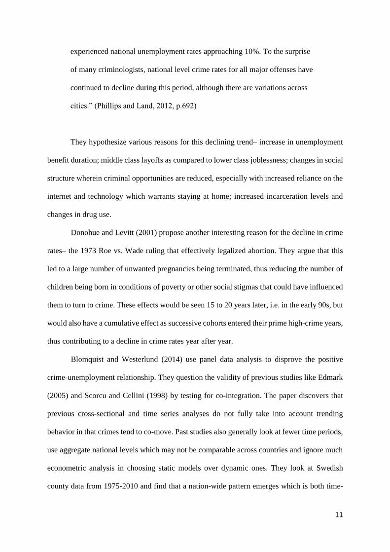
The fixed effect estimates of Model (1) in column 2 of Table 1 are reported again in column
1 of Table 2. Column 2 of Table 2 reports the fixed effect estimates of Model (2). As can be
seen, the estimate of 3 with an expected sign is significant, indicating that an increase in the
enrollment rate reduces property crime. However, the estimates of 4 and 5 are not
significantly different from zero, indicating that both firearm checks and law enforcement
officials per capita do not significantly affect property crime. Accordingly, we exclude these
control variables and rerun the model with the results reported in column 3 of Table 2:
Pit = 0 + 1D*Uit-1+ 2(1-D)*Uit-1 + 3Eit + µit (3)
4 The enrollment rate variable includes White, African-American and Hispanic students. 5 http://nces.ed.gov/ccd/elsi/expressTables.aspx
6 https://www.fbi.gov/about-us/cjis/nics/reports/nics_firearm_checks_-_year_by_state_type.pdf
17
Table 2: Fixed effect model estimates
Notes: Numbers in parentheses are absolute t-rations calculating using Newey- West Standard Errors.
Model 1 Model 2 Model 3
D* Uit-1
(1-D)* Uit-1
Control variables:
Eit
FCit
LEOit
0.494 (3.368)
0.795 (3.487)
-
-
-
0.485 (2.851)
0.950 (3.761)
-1.522 (1.866)
0.003 (0.001)
1.259 (0.996)
0.434 (2.760)
0.878 (3.601)
-1.456 (1.811)
-
-
Standard Error of Regression 4.629 4.553 4.543
Wald test p-value
(H0: ß1= ß2)
0.003 0.001 0.002
Observations
(Years=9, States=51)
457 457 457

18
Again, the Wald test, with a p-value 0.002 < 1% level of significance leads us to reject the
null hypothesis that 1= 2. This again means that asymmetry does indeed exist in the
unemployment-property crime relationship, subject to economic downturns. Specifically, as
before, the effect of unemployment on property crime is more pronounced during periods of
stable economic growth. During economic downturns, we see a reduced positive effect of
unemployment on property crime.
We also see that increased enrollment has a negative effect on property crime, as the
literature suggests (Scorcu and Cellini, 1998). However, it is worthwhile for future studies to
look at these enrollment rates divided by race. Does an increase in enrollment of children of
African-American or Hispanic descent have a greater impact than an increase in enrollment of
white children, for example?
The literature surveyed has specific suggestions for the inclusion of complements to crime,
including alcohol, guns and drugs (Phillips and Land, 2012). Data for alcohol consumption and
drug abuse proved difficult to find for the specified time period and geographic units. However,
the NICS system reports proved to be useful as they effectively constitute a gun registry. Every
time a customer walks up to a gun seller, the seller is required to run an obligatory background
check on him/her. These checks go through the NICS system, so as to look at previous criminal
history, history of mental health problems or drug abuse and the like. Not all checks necessarily
result in the gun being sold, however, these do constitute the only official data source on the
number of registered guns in the economy. It could be hypothesized that the number of firearm
checks are positively related to the crime rate. However, it is also likely that there is no
statistical significance to that relationship as it could be argued that crimes are not necessarily
committed by those who have registered firearms, but rather, those who possess illegal,
unregistered ones. This notion is what our model provides support for, as there is no statistically
significant link between firearm checks and property crime rate.

19
The presence of law enforcement officials per state is expected to decrease crime rates,
as per theory from economics and criminology (Chiricos, 1987). In such a scenario, it is useful
to see whether this theory truly holds up. However, is important to note that just the presence
of enforcement does not constitute an indicator of its effectiveness, which might be better
explained by solved crimes or arrests. Yet, for the purposes of our study, it is hypothesized that
since the number of law enforcement officials is the most visible hand of the law in action, that
too should provide a deterrent for property crime. This theory does not empirically hold up in
this study, since there is no statistically significant link between the number of law enforcement
officials and property crime. There may be a potential simultaneity issue involved with the
inclusion of such a variable, i.e., higher crime rates could also be the reason for more law
enforcement officials being employed by the state. We tried to account for this by testing the
lagged independent variable, and the results still hold. However, future studies would do well
to recognize the issues involved in such testing.
CONCLUSIONS
Our findings largely conform with previous literature in that we do see a positive
relationship between property crime and unemployment. However, the study also sheds light
on a surprising finding– the impact of unemployment on property crime rates is greater in stable
economic times than in periods of economic turmoil. We propose some reasons for this trend,
wherein the lack of target availability outstrips criminal motivation as per theories advanced
by Cantor and Land (1985).
The 2008 financial crisis resulted in large cyclical unemployment. People were laid off
from positions that required above average educational attainment, as opposed to chronic
unemployment. Such educated unemployed individuals would not necessarily resort to crime
as a way out of their situations–so a crime surge would not occur. Instead, what could have
happened was that there would be a decline in availability of targets for potential property

20
crimes, as the unemployed would be home more often and would be more prone to zealously
guarding whatever they had left– resulting in a decrease in property crime rates which would
be more in tune with the general trend of crime rates all over the world, and in USA in particular
(Cook and Wilson, 1985).
A more nuanced psychological reasoning can be employed in order to interpret these
results– in stable economic times, the impact of losing one’s job is felt much more acutely than
in a recession where everyone is suffering. In such a situation, one would turn to last-ditch
measures like thievery more easily when everyone around him/her was doing better than when
everyone was in the same boat. Wilkin (2015) calls this an “equity restoration behavior”,
wherein unequal distributions lead to frustration and a sense of trying to restore the balance,
while equal distributions, like the ones produced in a recession, would constitute “distributive
justice”. Wilkin (2015) also puts forward the view that if an individual were to lose his/her job,
he/she would be more likely to be driven to self-harm or domestic violence rather than manifest
desperation in more overt actions like stealing, which would make him/her easily prone to
being caught by the police. This would be even more apparent in a recession where the
probability of finding a new job was greatly reduced, desperations would run high and
therefore, “disappointed individuals would be more likely to quit or withdraw because although
they expected a positive outcome, they have unmet expectations and feel powerless” (Wilkin,
2015, p.161). Wilkin believes that these individuals would be unlikely to resort to stealing in
order to cope with such emotions.
In terms of education being linked to lower rates of crime, Lochner and Moretti (2004)
find a clear link between changes in schooling laws in US states that increased access to
education, and a reduction in incarceration and arrest rates. They use high school graduation
rates as a proxy, while we use enrollment rates, defined as the total number of students enrolled
in public schools in each state. Enrollment rates do not necessarily capture attainment,

21
however, they do give us a valuable understanding of whether just being part of an educational
system helps in reducing crime. We find a negative link between property crime rates and
enrollment rates, thus providing support for this view. There are many other control variables
that could have been added to make the model more robust, namely– age and race variables,
population living under the poverty line, worker incomes etc. Data for these for the time period
studied are not available, as they come from Census data that is only collected every five years
or so. However, future studies could benefit from adding such controls. Indeed, increased
emphasis must be placed on making education available to children from disadvantaged
backgrounds. Racial discrimination too plays an important role in contributing to continued
social inequality, and in the absence of policies such as affirmative action that level the playing
field, these children could be sucked into a continuing spiral of crime and illegal activities.
Finally, we turn to the control variables that were statistically insignificant– firearm
checks and law enforcement officials. Specifically, this study finds no significant link between
property crime and the number of registered gun checks. Although this link is tenuous at best,
with firearms being complements to violent crime rather than property crime, it is worthwhile
to conduct more detailed studies with better data on the link between guns and crime. As
mentioned before, premeditated or repeat crimes are probably not committed with registered
guns, and it is almost impossible to get data on actual gun sales owing to a large underground
market. Similarly, we find no statistically significant link between the number of police officers
and property crime. Property crimes by nature are stealthier and more advanced than violent
crimes, which makes personal surveillance more important, rather than police surveillance.
Also, an increase in law enforcement could be caused by an increase in crime as well, leading
to a simultaneity problem that is hard to correct or account for.

22
REFERENCES
Altindag, D. (2012). Crime and unemployment: Evidence from Europe. International Review
of Law and Economics, 32(1), 145-157.
Blomquist, J., and Westerlund, J. (2014). A non-stationary panel data investigation of the
unemployment–crime relationship. Social Science Research, 114-125.
Cantor, D., and Land, K. (1985). Unemployment and Crime Rates in the Post-World War II
United States: A Theoretical and Empirical Analysis. American Sociological Review,
50(3), 317-332.
Chiricos, T. (1987). Rates of Crime and Unemployment: An Analysis of Aggregate Research
Evidence. Social Problems, 34(2), 187-212.
Cook, P., and Wilson, J. (1985). Unemployment and Crime- What is the Connection? The
Public Interest, 79, 3-8.
Donohue, J. J., and Levitt, S. D. (2001). The Impact of Legalized Abortion on Crime. The
Quarterly Journal of Economics, 116(2), 379–420.
Edmark, K. (2005). Unemployment and Crime: Is There a Connection? The Scandinavian
Journal of Economics, 107(2), 353-373.
Levitt, S. (2001). Alternative Strategies for Identifying the Link Between Unemployment and
Crime. Journal of Quantitative Criminology, 17(4).
Lochner, L., and Moretti, E. (2004). The Effect of Education on Crime: Evidence from Prison
Inmates, Arrests, and Self-Reports. American Economic Review, 94(1), 155-189.
Phillips, J., and Land, K. (2012). The link between unemployment and crime rate fluctuations:
An analysis at the county, state, and national levels. Social Science Research, 41(3), 681-
694.
Raphael, S., and Winter‐ Ebmer, R. (2001). Identifying the Effect of Unemployment on Crime.
The Journal of Law and Economics, 44(1), 259-283.

23
Scorcu, A., and Cellini, R. (1998). Economic activity and crime in the long run: An empirical
investigation on aggregate data from Italy, 1951–1994. International Review of Law and
Economics, 18(3), 279-292.
Wilkin, C., and Connelly, C. (2015). Green with envy and nerves of steel: Moderated mediation
between distributive justice and theft. Personality and Individual Differences, 72, 160-
164.
24
QUANTIFYING THE OIL PRICE PLUNGE
Husain Rangwalla
School of Business Administration
American Univeristy of Sharjah
E-mail: [email protected]
ABSTRACT
From early June 2014 until date, the global economy has experienced a sudden,
unexpected and rather intriguing drop in oil prices. In spite of the extensive research in this
field, the question of why oil prices have plunged remains unanswered. Additionally, amidst
the umpteen determinants driving oil prices and their speculations, no single factor remains
solely attributable to the same. This paper will attempt at providing an explanation to the
current crisis by running a quantitative analysis on the potential factors driving the recent trend
in the oil prices. Given the insight derived from the quantitative analysis, this paper will make
policy recommendations to sustain the plunge and reverse the trend through substantive and
constructive policy action. Not only will this avoid a replay of the mid 1980’s oil crisis but also
provide an economic stimulus to avoid economic turmoil and entrenchment in the long-run.

25
INTRODUCTION
From early June 2014 until date, the global economy has experienced a sudden,
unexpected and rather intriguing drop in oil prices. To explain the same, there have been
misleading theories on oil prices aimed at destabilizing the Russian economy (Gladstone &
Krauss, 2015) or bringing economic insecurities to the Iranian drilling efforts (Gause, 2015).
On the other hand, there has been extensive economic research conducted to identify and
explain the economic drivers of the plunging oil prices but with limited success.
Figure 1. The First derivative Change in Oil Prices ($/barrel).
The 1980’s saw a similar stagnation in oil prices which was followed by a sudden drop
of over 67% in a four-month window (Loder, 2014). The sudden plunge in this historical crisis
was triggered by a price war orchestrated by Saudi Arabia which created negative global
implications. While U.S. industrialization faced the major brunt of the uncalled for
competition, global economic activity slipped into a trough until the mid-1990’s (Gately, 1986,
26
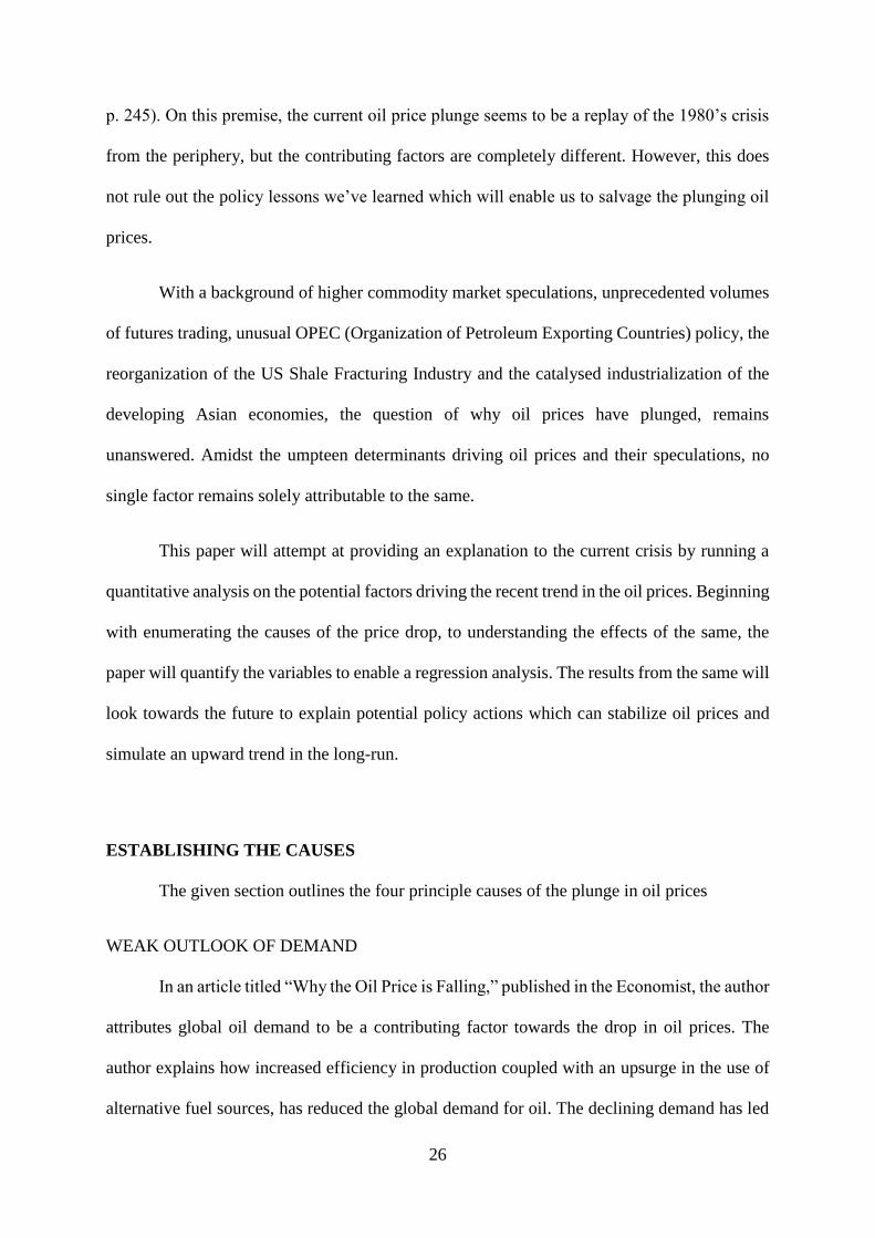
p. 245). On this premise, the current oil price plunge seems to be a replay of the 1980’s crisis
from the periphery, but the contributing factors are completely different. However, this does
not rule out the policy lessons we’ve learned which will enable us to salvage the plunging oil
prices.
With a background of higher commodity market speculations, unprecedented volumes
of futures trading, unusual OPEC (Organization of Petroleum Exporting Countries) policy, the
reorganization of the US Shale Fracturing Industry and the catalysed industrialization of the
developing Asian economies, the question of why oil prices have plunged, remains
unanswered. Amidst the umpteen determinants driving oil prices and their speculations, no
single factor remains solely attributable to the same.
This paper will attempt at providing an explanation to the current crisis by running a
quantitative analysis on the potential factors driving the recent trend in the oil prices. Beginning
with enumerating the causes of the price drop, to understanding the effects of the same, the
paper will quantify the variables to enable a regression analysis. The results from the same will
look towards the future to explain potential policy actions which can stabilize oil prices and
simulate an upward trend in the long-run.
ESTABLISHING THE CAUSES
The given section outlines the four principle causes of the plunge in oil prices
WEAK OUTLOOK OF DEMAND
In an article titled “Why the Oil Price is Falling,” published in the Economist, the author
attributes global oil demand to be a contributing factor towards the drop in oil prices. The
author explains how increased efficiency in production coupled with an upsurge in the use of
alternative fuel sources, has reduced the global demand for oil. The declining demand has led
27
to the initial drop in oil prices and which has resulted in a further ‘investment drought’ in the
oil and gas sector of the economy. This weak economic outlook of the oil and gas sector has
further aggravated the drop in oil prices.
Looking ahead, an article titled “Global Oil Demand Growth to Slow down in 2016,”
published in The Wall Street Journal expects the economic uncertainties to prevail maintaining
the weak demand and further dropping the oil prices if not for any structural adjustments.
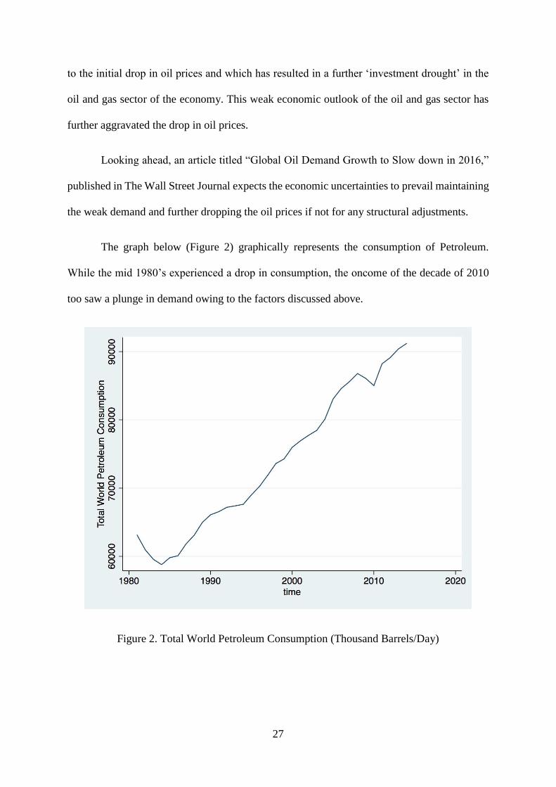
The graph below (Figure 2) graphically represents the consumption of Petroleum.
While the mid 1980’s experienced a drop in consumption, the oncome of the decade of 2010
too saw a plunge in demand owing to the factors discussed above.
Figure 2. Total World Petroleum Consumption (Thousand Barrels/Day)
28
CURRENT STATE OF OVERSUPPLY
In an article titled “Oil Prices Could Keep Falling Due to Oversupply, Says IEA,”
published by The Guardian, three factors have been accounted as responsible for the
oversupply of oil in the global markets. Firstly, the exploration of oil fields followed by drilling
in Venezuela and Nigeria. Secondly, the quickly growing US Shale Fracturing and lastly the
falling demand for oil. However, these factors could have been balanced out by adjustments in
the OPEC Supply Policies, if not for the tough stance of Saudi Arabia.
Amidst the current state of oversupply, in an article titled “Oil Demand Growth to Slow,
IEA says, but is OPEC Listening,” published by C.N.B.C., Holly Ellyatt blames the OPEC for
lack of policy action after sighting selfish incentives during the time of a commodity crisis.
While the OPEC cartel can single-handedly rebalance the oil market towards equilibrium, the
OPEC refuses to do so in order to drive the oil-dependent economies like Russia and Brazil out
of business and capture their market share in turn. Therefore we see that oversupply will remain
an upward trend creating further stimulus for falling oil prices.
The graph (Figure 4) explains the accelerated increase in oil in the years 2012-2014.
This oversupply, as explained above is a potential cause of the current plunge in prices.

29
Figure 3. Total World Oil Supply (Thousand Barrels/ Day).
APPRECIATION OF US DOLLAR
In an article titled “Crude Oil Prices Fell Due to the Appreciating US Dollar,” published
by Market Realist, the high volumes of appreciation in the US dollar have laid heavy stress on
the dollar denominated oil prices. There has been a 10% appreciation in the US Dollar relative
to the major trade-weighted currencies in the world (World Bank, 2015). This increase in prices
encompasses the first two factors of the oil plunge. Firstly, decreasing demand through a
reduced purchasing power globally and secondly, increasing supply through higher export
margins. Thus the appreciation of the US Dollar has had a multi-fold impact on oil prices during
2014-2015.
PRICE OUTLOOK OF OIL
In a report titled “The Great Plunge in Oil Prices: Causes, Consequences and Policy
Responses,” published by the World Bank, the price outlook of oil is a factor which directs the

30
trend in oil prices. This is to say that prior to the plunge high oil prices forced substitution to
biofuels and solar power. After the plunge, shale fracturing halted majority operations. Both
these events are different in their audiences and effects but similar in their long term horizon
which requires immediate reversal through sustainable policy action.
QUANTIFYING THE DETERMINANTS
This paper will now quantify the factors contributing towards the determination and
plunge in the oil prices. A period of 34 years will be considered from 1981-2014. This period
of time is characterized by 3 major fluctuations in oil prices, the 1980’s crisis, the recession of
2007-08 and lastly, the recent oil price plunge of 2014.
GLOBAL OIL SUPPLY
U.S. Energy Information Administration
The Global Oil Supply in Thousand Barrels per Day will be obtained from the dataset
provided by E.I.A. This dataset will be treated as four individual variables:
1. Global Oil Supply: This variable will add an overall outlook to the effect of supply on
global oil prices
2. O.P.E.C. Oil Supply: This variable will represent the OPEC Export and Production
policies.
3. O.E.C.D. Oil Supply: this variable will represent the new entrants and increase in
production as well as supply in the OECD countries.
4. U.S. Oil Supply: This variable will represent the major effect of Shale Fracturing on
global oil prices.
GLOBAL PETROLEUM CONSUMPTION
U.S. Energy Information Administration

31
The Global Petroleum Consumption in Thousand Barrels per Day will be obtained from
the dataset provided by E.I.A. This dataset will be treated as three individual variables:
1. Global Petroleum Consumption: This variable will represent the overall outlook of
global oil demand and consumption patterns.
2. Asia & Oceanic Petroleum Consumption: This variable will represent the growing
oil consumption in the developing nations of south-east Asia and the Far East
3. China Petroleum Consumption: This variable will account for the massive growth of
Chinese industrialization which has contributed significantly towards the global oil
demand.
OIL RENTS AS A PERCENTAGE OF GDP
The World Bank
“Oil rents are the difference between the value of crude oil production at world prices and
total costs of production” (World Bank, 2011). This dataset will be treated as three individual
variables:
1. China’s Oil Rents as % of GDP: China being the biggest economy in the East is used
as a representative variable in this section.
2. US’ Oil Rents as % of GDP: US Shale Gas Rents which make US the current largest
producer of oil are represented by this variable.
3. Saudi Arabia’s Oil Rents as % of GDP: The world’s former largest oil producer’s
income is represented in this variable.
CRUDE OIL RESERVES
U.S. Energy Information Administration
The Crude Oil Reserves in billion barrels will be obtained from the dataset provided by
E.I.A. This dataset will be treated as three individual variables:
32
1. World Crude Oil Reserves: This variable will be representative of the global crude
oil stock.
2. O.P.E.C. Crude Oil Reserves: This variable will represent the OPEC reserves, which
is a source of bargaining power for the cartel.
3. O.E.C.D. Crude Oil Reserves: This variable represents the limited reserves held by
the OECD cartel, which makes it vulnerable to the current crisis.
OIL IMPORTS AS A PERCENTAGE OF GDP
The World Bank
From the global data set a single variable will be used:
1. U.S. Oil Imports as a % of GDP: Until off-late, the U.S. used to be the biggest oil
importer of the world which laid sufficient influence on the pricing of the oil barrel.
This variable will represent the same.
U.S. DOLLAR VALUE AS COMPARED TO OTHER CURRENCY UNITS
The World Bank
From this comprehensive currency comparison dataset a single variable will be used:
1. U.S. Dollar Value as compared to the British Pound: This variable will help study
the effect of the U.S. Dollar Appreciation on the recent oil plunge.
ALTERNATE ENERGY AND NUCLEAR ENERGY AS A PERCENTAGE OF ENERGY
USE
The World Bank
This single variable will help study the effect of alternate energy sources on the demand
and pricing of the oil barrel.
33
WORLD INFLATION INDICES
The World Bank
A single variable of U.S. Inflation will be used from the dataset to represent the
contribution of the overall increase of prices in the economy as compared to oil.
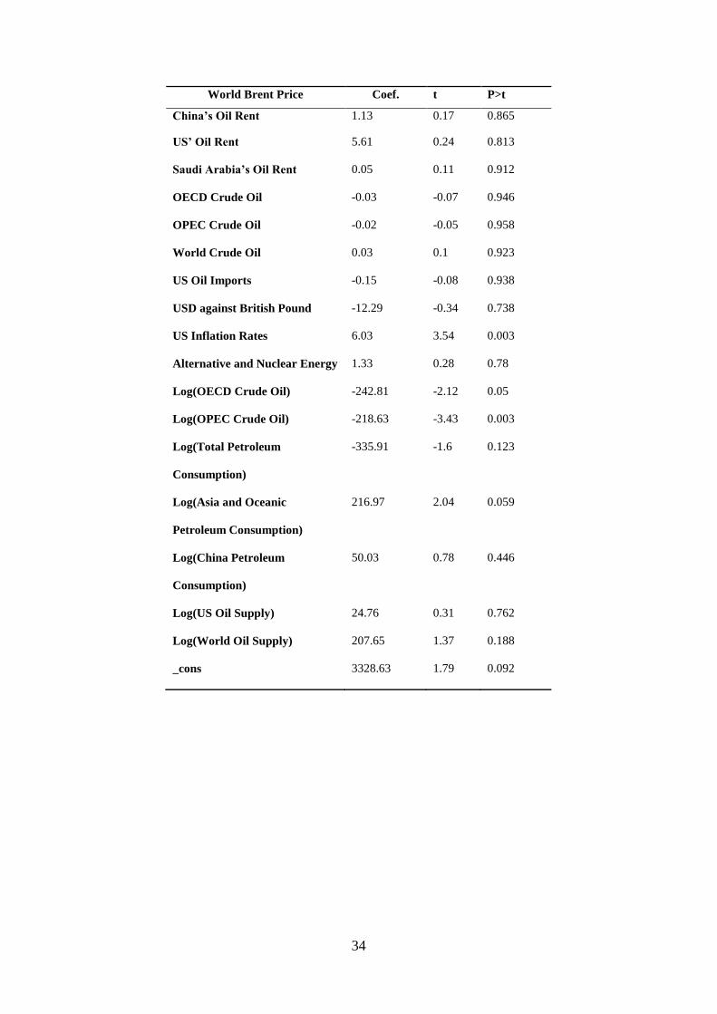
DATA ANALYSIS
Given the following independent variables, we regress them with the dependent
variable, World Brent Price, to understand the contribution of each determinant towards the
changes in oil prices. We use Stata to perform the operation and receive the following results.
UNDERSTANDING THE SIGNIFICANT VARIABLES
US INFLATION RATES
The U.S. Inflation Rate has a significant and a positive output on the price of oil.
Economically, inflation is a positive indicator of economic activity. According to Philip’s
Curve an economy closer to full employment will have a higher inflation rate. Therefore, to
explain the $6.03 increase for every 1 point increase in inflation, the economy features higher
employment, resulting in higher economic activity, which requires more oil. An increase in the
demand of oil, by the law of demand increases the price of oil.
OECD OIL SUPPLY & OPEC OIL SUPPLY
Both the given variables have a negative impact on the price of oil. For every 1 million
barrels per day increase in oil supply from OECD and OPEC, the price of oil would drop by
$242 and $218 respectively. This operation does not occur in isolation though. Coupled with
increased demand as a stimulus, decreasing reserves as a result the impact of
34
World Brent Price Coef. t P>t
China’s Oil Rent 1.13 0.17 0.865
US’ Oil Rent 5.61 0.24 0.813
Saudi Arabia’s Oil Rent 0.05 0.11 0.912
OECD Crude Oil -0.03 -0.07 0.946
OPEC Crude Oil -0.02 -0.05 0.958
World Crude Oil 0.03 0.1 0.923
US Oil Imports -0.15 -0.08 0.938
USD against British Pound -12.29 -0.34 0.738
US Inflation Rates 6.03 3.54 0.003
Alternative and Nuclear Energy 1.33 0.28 0.78
Log(OECD Crude Oil) -242.81 -2.12 0.05
Log(OPEC Crude Oil) -218.63 -3.43 0.003
Log(Total Petroleum
Consumption)
-335.91 -1.6 0.123
Log(Asia and Oceanic
Petroleum Consumption)
216.97 2.04 0.059
Log(China Petroleum
Consumption)
50.03 0.78 0.446
Log(US Oil Supply) 24.76 0.31 0.762
Log(World Oil Supply) 207.65 1.37 0.188
_cons 3328.63 1.79 0.092
35
the increase in supply would be considerably lesser. However, the negative coefficient
highlights the argument of an oil price plunge owing to the oversupply of oil by the OPEC.
ASIA AND OCEANIC PETROLEUM CONSUMPTION
According to the regression coefficient for every million barrels per day increase in the
consumption of the Asia and Oceanic Petrol Consumption, oil prices will increase by $217. In
lines with the economic theory of demand, this is a plausible claim. On the other hand, given
that the demand for oil in this region is growing but at a declining rate, this contributes towards
the current oil plunge. With the increased use of alternate fuels and efficient technology, the
developing world is reducing its dependence on oil.
TESTING FOR SERIAL CORRELATION
Given that we are using a time-series dataset, we use the Breusch Godfrey test for serial
correlation. In the context of the research question we conduct the test using a 10 period (year)
lag variable, to test for the null hypothesis claiming no serial correlation. Given a low p-value,
we reject the null hypothesis of no serial correlation. The presence of serial correlation by
definition implies that past values of a time-series dataset, set a trend to be repeated in the
future. Hence, as stated earlier we can use policy lessons and defence mechanisms from the
1985-86 oil plunge to stabilize oil prices and stimulate an upward trend at the earliest.
POLICY IMPLICATIONS AND RECOMMENDATIONS
Given the insight derived from the significant variables in the data analysis in the earlier
section, this section will make policy recommendations to sustain the plunge and reverse the
trend through substantive and constructive policy action.
MONETARY POLICY
Oil plays the role of an intermediate good in every production process. Given the
decrease in oil prices, production costs will decrease, which will be shortly followed by a
36
decrease in prices to the benefit of consumers. However, the drop in prices will initially ease
inflation only to add deflationary pressures to the economy in the longer run. In the case of
sticky prices, a sustained price drop will only create further turmoil in the economy (World
Bank, 2015).
Given the linear relation between inflation and oil prices, inflation must be maintained
to aid a pleasant recovery of oil prices. Therefore, from the monetary policy standpoint, the
money supply in the economy must be increased coupled with lower interest rate targeting to
maintain economic momentum and increase the energy use via catalysed economic activity.
FISCAL POLICY
As explained by a report titled “The Great Plunge in Oil Prices,” published by the World
Bank in 2015, low oil prices create opportunity for radical fiscal reform. Given the lower oil
prices, subsidies on oil can be redirected towards infrastructural development which can boost
economic activity and increase the investment attractiveness of an economy. Additionally, as
explained by the same report, investments should be directed towards the energy sector as
opposed to liquidation, to create sufficient stimulus to boost demand for oil in the global energy
use index (World Bank, 2015, p.42).
CONCLUSION
The role of the governments and economists of the world is to take immediate action
to prevent a downturn of events as previously experienced in the mid-1980s. Given a recent
recovery from the Great Recession of 2007-08, another crisis would spell danger for the
developing as well as the developed economies of the world. As the price trend could mirror
in other commodity markets too, recovery will be a harder and longer economic process.
Therefore, given the extensive research, to re-emphasize the objectives of the paper, immediate
fiscal and monetary policy actions must be taken coupled with untiring lobbying efforts to

37
curtail the supply by the oil cartels in existence. In light of sufficient economic stimulus, a
decade of economic entrenchment will be unnecessary.

38
REFERENCES
Baffes, J. (2015). The great plunge in oil prices causes, consequences, and policy
responses. Washington, D.C.: World Bank Group, Development Economics.
EIA short-term US Energy outlook. (2015, December 8). U.S Energy Information
Administration. Retrieved January 7, 2016, from http://www.eia.gov/forecasts/steo/
Ellyatt, H. (2015, October 13). Oil demand growth to slow, IEA says, but is OPEC listening?
CNBC. Retrieved January 7, 2016, from http://www.cnbc.com/2015/10/13/oil-
demand-growth-to-slow-iea-says-but-is-opec-listening.html
Energy imports, net (% of energy use). (n.d.). Retrieved January 7, 2016, from
http://data.worldbank.org/indicator/EG.IMP.CONS.ZS
Gold, R. (2015, January 13). Back to the Future? Oil Replays 1980s Bust. The Wall Street
Journal. Retrieved January 7, 2016, from http://www.wsj.com/articles/back-to-the-
future-oil-replays-1980s-bust-1421196361
International Energy Statistics - EIA. (n.d.). Retrieved January 7, 2016, from
https://www.eia.gov/cfapps/ipdbproject/IEDIndex3.cfm?tid=5&pid=53&aid=1
International Energy Statistics - EIA. (n.d.). Retrieved January 7, 2016, from
https://www.eia.gov/cfapps/ipdbproject/IEDIndex3.cfm?tid=5&pid=5&aid=2
International Energy Statistics - EIA. (n.d.). Retrieved January 7, 2016, from
https://www.eia.gov/cfapps/ipdbproject/IEDIndex3.cfm?tid=5&pid=57&aid=6
Iran oil minister blames OPEC oversupply for low crude prices. (2015, December 6). Reuters.
Retrieved January 7, 2016, from http://www.reuters.com/article/iran-opec-
idUSL8N13V09I20151206

39
Krauss, C., & Gladstone, R. (2015, August 24). From Venezuela to Iraq to Russia, Oil Price
Drops Raise Fears of Unrest. The New York Times. Retrieved January 7, 2016, from
http://www.nytimes.com/2015/08/25/world/from-venezuela-to-iraq-to-russia-oil-
price-drops-raise-fears-of-unrest.html?_r=0
Kristopher, G. (2015, November 18). Crude Oil Prices Fell Due to the Appreciating US Dollar.
Crude Oil Market: Bearish Traders Fed by More Supply News. Retrieved January 7,
2016, from http://marketrealist.com/2015/11/crude-oil-prices-fall-due-appreciating-
us-dollar/
Loder, A. (2014, November 26). Oil Bust of 1986 Reminds U.S. Drillers of Price War Risks.
Bloomberg Buisness. Retrieved January 7, 2016, from
http://www.bloomberg.com/news/articles/2014-11-26/oil-bust-of-1986-reminds-u-s-
drillers-of-price-war-risks
Official exchange rate (LCU per US$, period average). (n.d.). Retrieved January 7, 2016, from
http://data.worldbank.org/indicator/PA.NUS.FCRF
Oil prices could keep falling due to oversupply, says IEA. (2015, July 10). The Guardian.
Retrieved January 7, 2016, from
http://www.theguardian.com/business/2015/jul/10/oil-prices-keep-falling-
international-energy-agency-oversupply
Oil rents (% of GDP). (n.d.). Retrieved January 7, 2016, from
http://data.worldbank.org/indicator/NY.GDP.PETR.RT.ZS
Said, S. (2015, November 13). Global Oil Demand Growth to Slow in 2016, IEA Says. The
Wall Street Journal. Retrieved January 7, 2016, from

40
http://www.wsj.com/articles/global-oil-demand-growth-to-slow-in-2016-iea-says-
1447405406
Why the oil price is falling. (2014, December 8). The Economist. Retrieved January 7, 2016,
from http://www.economist.com/node/21635751/print

41
A CROSS-COUNTRY PANEL STUDY OF THE RELATIONSHIP BETWEEN
URBANIZATION AND SUICIDE IN JAPAN AND KOREA
Jason Torion
School of Business Administration
American University of Sharjah
Email: [email protected]
ABSTRACT
Suicide has not been a major global issue until recently. Over the years, suicide
incidents have risen steeply and research is still being conducted on the causes. Increasing
suicide rates reflect a society’s mental wellbeing and in some countries it could be, in fact,
considered a norm to see so many suicide incidents reported on the news. Japan and the
Republic of Korea (South Korea) are known to both have the highest suicide rates in the Asian
Region. Japan ranks 9th in the world, and South Korea follows at 10th in an International Suicide
Statistics Ranking published by the World Health Organization. These two countries are also
the only two Asian countries in the top ten ranking, with the rest of the other eight countries
being European. Despite both being two of the most economically developed countries in Asia,
their alarmingly high suicide rates suggest that their population’s mental health has degraded
over the years. This paper will empirically explore the economic reasons, if any, behind the
high suicide rates with panel data evidence from 1991 to 2010. The main focus will be
confirming the impact of increased urban population (urbanization) on suicide rates in
comparison to other economic and socio-economic facts such as unemployment, individual
(average) income levels, alcohol consumption and the like, in order to validate various
literature and empirical studies conducted on the topic.

42
LITERATURE REVIEW
Majority of the literature published consider unemployment and individual income
levels the main two indicators behind increasing suicide rates. Noh (2009) states that individual
income levels can be used to explain the population’s level of happiness. Higher income levels
could be correlated with lower suicide rates but it should be their relative income (i.e. GDP
per Capita growth rate) because “happiness is affected more by one’s sense of relative income
than by absolute income”.
Shah (2008) and his findings on Urbanization and Suicide Rate in the Elderly
Population was part of the motivation behind this research paper. Shah conducts his study on
the underlying premise that ‘Urbanization’ leads to the weakening of family ties and social
bonds, including bonds with local religious societies. These, alongside the difficulties in
adjusting towards urban lifestyles are all possible reasons towards increased suicide rates.
Although this study was geared towards the Elderly Population, I will be adopting a similar
perspective in this paper. Interestingly, Oguro & Kaido (2009) find that Japan has a reputation
of being a ‘Suicide Society’ and find that social factors play a huge part in the alarming increase
in suicide rates in Japan alone. Unfortunately, trustworthy data on social factors are very
difficult to find and aggregate, hence ‘Urbanization’, along with fertility rate and female
participation in the labor force will be used to control for social factors instead.
Shah (2010) discusses the conflicting results from various authors. Results vary from
positive, negative, or no relationship between urbanization and suicide incidents. Stack (2000)
proposes a curvilinear relationship model to explain the conflicting findings but as Shah (2010)
replicates this model with much more recent data, he finds that there is an absence of such a
relationship.
43
DATA
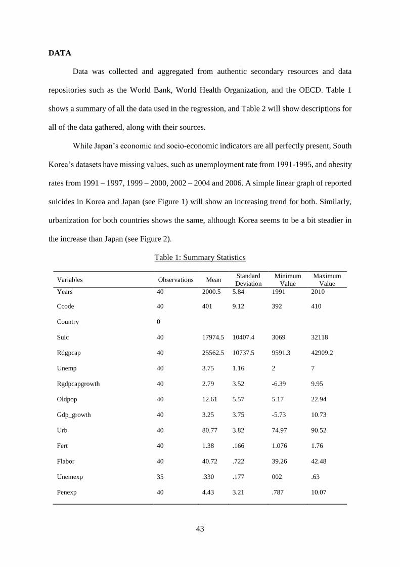
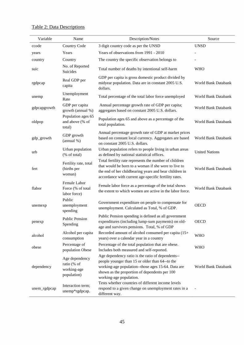
Data was collected and aggregated from authentic secondary resources and data
repositories such as the World Bank, World Health Organization, and the OECD. Table 1
shows a summary of all the data used in the regression, and Table 2 will show descriptions for
all of the data gathered, along with their sources.
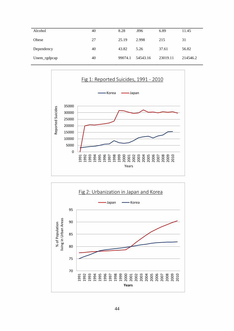
While Japan’s economic and socio-economic indicators are all perfectly present, South
Korea’s datasets have missing values, such as unemployment rate from 1991-1995, and obesity
rates from 1991 – 1997, 1999 – 2000, 2002 – 2004 and 2006. A simple linear graph of reported
suicides in Korea and Japan (see Figure 1) will show an increasing trend for both. Similarly,
urbanization for both countries shows the same, although Korea seems to be a bit steadier in
the increase than Japan (see Figure 2).
Table 1: Summary Statistics
Variables Observations Mean Standard
Deviation
Minimum
Value
Maximum
Value
Years 40 2000.5 5.84 1991 2010
Ccode 40 401 9.12 392 410
Country 0
Suic 40 17974.5 10407.4 3069 32118
Rdgpcap 40 25562.5 10737.5 9591.3 42909.2
Unemp 40 3.75 1.16 2 7
Rgdpcapgrowth 40 2.79 3.52 -6.39 9.95
Oldpop 40 12.61 5.57 5.17 22.94
Gdp_growth 40 3.25 3.75 -5.73 10.73
Urb 40 80.77 3.82 74.97 90.52
Fert 40 1.38 .166 1.076 1.76
Flabor 40 40.72 .722 39.26 42.48
Unemexp 35 .330 .177 002 .63
Penexp 40 4.43 3.21 .787 10.07
44
Alcohol 40 8.28 .896 6.89 11.45
Obese 27 25.19 2.998 215 31
Dependency 40 43.82 5.26 37.61 56.82
Unem_rgdpcap 40 99074.1 54543.16 23019.11 214546.2
0
5000
10000
15000
20000
25000
30000
35000
19
91
19
92
19
93
19
94
19
95
19
96
19
97
19
98
19
99
20
00
20
01
20
02
20
03
20
04
20
05
20
06
20
07
20
08
20
09
20
10
Rep
ort
ed S
uic
ides
Years
Fig 1: Reported Suicides, 1991 - 2010
Korea Japan
70
75
80
85
90
95
19
91
19
92
19
93
19
94
19
95
19
96
19
97
19
98
19
99
20
00
20
01
20
02
20
03
20
04
20
05
20
06
20
07
20
08
20
09
20
10
% o
f P
op
ula
tio
n
livin
g in
Urb
an A
reas
Years
Fig 2: Urbanization in Japan and Korea
Japan Korea
45
Table 2: Data Descriptions
Variable Name Description/Notes Source
ccode Country Code 3 digit country code as per the UNSD UNSD
years Years Years of observations from 1991 - 2010 -
country Country The country the specific observation belongs to -
suic No. of Reported
Suicides Total number of deaths by intentional self-harm WHO
rgdpcap Real GDP per
capita
GDP per capita is gross domestic product divided by
midyear population. Data are in constant 2005 U.S.
dollars.
World Bank Databank
unemp Unemployment
Rate Total percentage of the total labor force unemployed World Bank Databank
gdpcapgrowth GDP per capita
growth (annual %)
Annual percentage growth rate of GDP per capita;
aggregates based on constant 2005 U.S. dollars. World Bank Databank
oldpop
Population ages 65
and above (% of
total)
Population ages 65 and above as a percentage of the
total population. World Bank Databank
gdp_growth GDP growth
(annual %)
Annual percentage growth rate of GDP at market prices
based on constant local currency. Aggregates are based
on constant 2005 U.S. dollars.
World Bank Databank
urb Urban population
(% of total)
Urban population refers to people living in urban areas
as defined by national statistical offices. United Nations
fert
Fertility rate, total
(births per
woman)
Total fertility rate represents the number of children
that would be born to a woman if she were to live to
the end of her childbearing years and bear children in
accordance with current age-specific fertility rates.
World Bank Databank
flabor
Female Labor
Force (% of total
labor force)
Female labor force as a percentage of the total shows
the extent to which women are active in the labor force. World Bank Databank
unemexp
Public
unemployment
spending
Government expenditure on people to compensate for
unemployment. Calculated as Total, % of GDP. OECD
penexp Public Pension
Spending
Public Pension spending is defined as all government
expenditures (including lump-sum payments) on old-
age and survivors pensions. Total, % of GDP
OECD
alcohol Alcohol per capita
consumption
Recorded amount of alcohol consumed per capita (15+
years) over a calendar year in a country WHO
obese Percentage of
population Obese
Percentage of the total population that are obese.
Includes both measured and self-reported. WHO
dependency
Age dependency
ratio (% of
working-age
population)
Age dependency ratio is the ratio of dependents--
people younger than 15 or older than 64--to the
working-age population--those ages 15-64. Data are
shown as the proportion of dependents per 100
working-age population.
World Bank Databank
unem_rgdpcap Interaction term;
unemp*rgdpcap.
Tests whether countries of different income levels
respond to a given change on unemployment rates in a
different way.
-
46
EMPIRICAL APPROACH
For Panel Data suitability, we use the random effects panel data model to estimate the
population model with the aforementioned variables with Suicide as the discrete dependent
variable. The use of the random effects model is determined through the Hausmann Test. We
are testing the hypothesis of whether or not urbanization, inclusive of all other economic and
socio-economic variables, is a possible cause and/or a major indicator of the increasing suicide
numbers in Japan and Korea. To deal with the issue of heteroscedasticity, we use Robust
Standard Errors during the regression. The variables used are similar to those that Noh (2009)
had used, with the exception of CO2 consumption – instead we use obesity rate as a proxy for
the country’s population’s health.
Theoretically, we expect a negative relationship between suicide and Real GDP per
Capita, Unemployment rate, GDP per Capita Growth, GDP Growth, Fertility Rates and
Government Expenditure on Unemployment and Pension. A positive relationship is expected
between suicide and urban population, alcohol consumption, obesity rate and age dependency
ratio. The expected effect of the elderly population and the interaction term are ambiguous. We
add an interaction variable between unemployment rate and real GDP per capita to control for
the difference in response of different income levels to a given change in unemployment rates
in different countries.
EMPIRICAL RESULTS
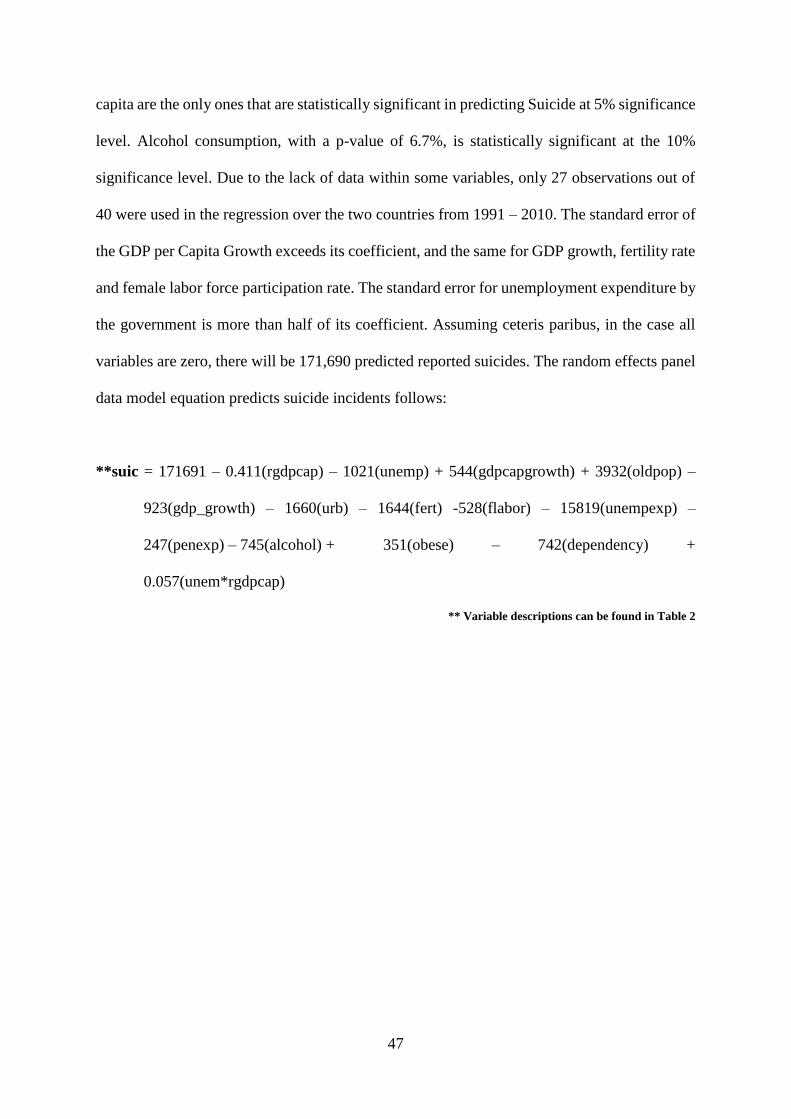
The regression results are as seen in Table 3. Overall, the independent variables explain
98% of the variations and/or changes in suicide incidents (R-squared). Out of the 14 predictors
used to predict suicide, the estimated coefficients of Real GDP per Capita, Unemployment
Rate, the elderly population, Urbanization, Government Expenditure on Unemployment and
Pension, as well as the interaction variable between unemployment rate and real GDP per
47
capita are the only ones that are statistically significant in predicting Suicide at 5% significance
level. Alcohol consumption, with a p-value of 6.7%, is statistically significant at the 10%
significance level. Due to the lack of data within some variables, only 27 observations out of
40 were used in the regression over the two countries from 1991 – 2010. The standard error of
the GDP per Capita Growth exceeds its coefficient, and the same for GDP growth, fertility rate
and female labor force participation rate. The standard error for unemployment expenditure by
the government is more than half of its coefficient. Assuming ceteris paribus, in the case all
variables are zero, there will be 171,690 predicted reported suicides. The random effects panel
data model equation predicts suicide incidents follows:
**suic = 171691 – 0.411(rgdpcap) – 1021(unemp) + 544(gdpcapgrowth) + 3932(oldpop) –
923(gdp_growth) – 1660(urb) – 1644(fert) -528(flabor) – 15819(unempexp) –
247(penexp) – 745(alcohol) + 351(obese) – 742(dependency) +
0.057(unem*rgdpcap)
** Variable descriptions can be found in Table 2
48
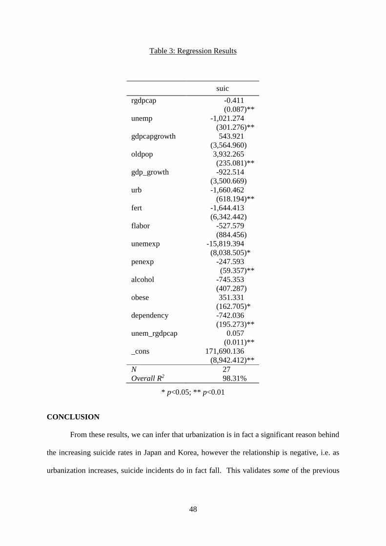
Table 3: Regression Results
* p<0.05; ** p<0.01
CONCLUSION
From these results, we can infer that urbanization is in fact a significant reason behind
the increasing suicide rates in Japan and Korea, however the relationship is negative, i.e. as
urbanization increases, suicide incidents do in fact fall. This validates some of the previous
suic
rgdpcap -0.411
(0.087)**
unemp -1,021.274
(301.276)**
gdpcapgrowth 543.921
(3,564.960)
oldpop 3,932.265
(235.081)**
gdp_growth -922.514
(3,500.669)
urb -1,660.462
(618.194)**
fert -1,644.413
(6,342.442)
flabor -527.579
(884.456)
unemexp -15,819.394
(8,038.505)*
penexp -247.593
(59.357)**
alcohol -745.353
(407.287)
obese 351.331
(162.705)*
dependency -742.036
(195.273)**
unem_rgdpcap 0.057
(0.011)**
_cons 171,690.136
(8,942.412)**
N
Overall R2
27
98.31%

49
studies that have concluded their research similarly (Otsu et al., 2004). As aforementioned,
many studies have also concluded with conflicting results.
However, this model may not be able to accurately predict suicide incidents. We have
missing values from obesity rates in Korea which could have greatly affected the results. Since
suicide is usually unpredictable, it has to do with a person’s mental wellbeing. A variable that
will proxy psychological factors should be used. Other than family help and social ties, another
variable should be added to determine a person’s religiousness, since it also affects a person’s
psychological state. In Japan and Korea, it is common to see mothers that have jobs
occasionally (part-time or temporary). Hence, unemployment rate and female labor force
participation (as well as dependency ratio) may not capture the effect needed to proxy for social
ties and family help since such mothers are usually housewives reported to be unemployed.
We suspect some endogeneity in the model as well. There could be a chance that as suicide
increases, alcohol consumption increases (from the friends and relatives left behind), which
could in turn also increase suicide. More investigation needs to be done on such predictors.
The model is also too widespread, i.e. we predicted it for the population as a whole. We
may be able to gain more insight by investigating and dividing data to predict suicides
separately between males and female. This result could also only be limited to Japan and Korea,
since they are both collectivist Asian Countries, perhaps other countries’ data should also be
added into the regression to get a more accurate model. An overall policy recommendation
would be for a government to ensure and secure government funds for pension and
unemployment expenditures should they want to reduce suicide incidents in their country.
50
REFERENCES
Hamermesh, Daniel S., & Soss, Neal M. (1974). An economic theory of suicide. Journal of
Political Economy. Retrieved from
http://www.jstor.org.ezproxy.aus.edu/stable/1830901?pq-origsite=summon
Noh, Y. (2009). Does unemployment increase suicide rates? The OECD Panel
Evidence. Journal of Economic Psychology, 30(4), 575-582. Retrieved from
http://www.sciencedirect.com.ezproxy.aus.edu/science/article/pii/S016748700900036
1
Oguro, J., & Kaigo, M. (2009). Suicide society: Media responsibility and suicide in Japan.
Media Asia, 36(1), 16-22. Retrieved from
http://ezproxy.aus.edu/login?url=http://search.proquest.com/docview/211508531?acc
ountid=16946
Otsu, A., Araki, S., Sakai, R., Yokoyama, K., & Scott Voorhees, A. (2004). Effects of
urbanization, economic development, and migration of workers on suicide mortality in
Japan. Social Science and Medicine. Retrieved from
http://www.sciencedirect.com.ezproxy.aus.edu/science/article/pii/S027795360300285
5
Shah, A. (2008). A cross-national study of the relationship between elderly suicide rates and
urbanization. Suicide & Life - Threatening Behavior, 38(6), 714-9. Retrieved from
http://ezproxy.aus.edu/login?url=http://search.proquest.com/docview/224878832?acc
ountid=16946

51
Shah, A. (2010). A replication of a cross-national study of the relationship between elderly
suicide rates and urbanization. International Psychogeriatrics, 22(1), 162-3. Retrieved
from http://search.proquest.com.ezproxy.aus.edu/docview/223739239?pq-
origsite=summon
S. Stack (2000). A replication of a cross-national study of the relationship between elderly
suicide rates and urbanization. Suicide and Life Threatening Behaviour, 30, 163-176.
The Organization for Economic Co-operation and Development (OECD). (2015). Government
Expenditure on Unemployment and Pension [Data file]. Available from
https://data.oecd.org/
The World Bank. (2015). World Development Indicators (1991-2010) for Japan and Republic
of Korea [Data file]. Available from http://data.worldbank.org/
World Health Organization. (2015). WHO Mortality Database [Data file]. Available from
http://www.who.int/healthinfo/statistics/mortality_rawdata/en/