Embed Size (px)
Citation preview

The Economics of Value Investing
Kewei Hou1 Haitao Mo2 Chen Xue3 Lu Zhang4
1The Ohio State University and CAFR
2Louisiana State University
3University of Cincinnati
4The Ohio State University and NBER
PBCSFDecember 11, 2017

IntroductionTheme
The investment CAPM reconciles the Graham-Dodd (1934)philosophy of value investing with neoclassical economics
Cross-sectionally varying expected returns, depending on �rms'investment, pro�tability, and expected investment growth
An appealing alternative to workhorse accounting models
An upgraded q-factor model augmented with an expectedinvestment growth factor (the Q5 model)

Outline
1 Security Analysis: Background
2 The Investment CAPM
3 Comparison with Accounting Models
4 The Expected Growth Factor

Outline
1 Security Analysis: Background
2 The Investment CAPM
3 Comparison with Accounting Models
4 The Expected Growth Factor

Security AnalysisClassics

Security AnalysisInvestment philosophy
Invest in undervalued securities selling well below the intrinsic value
The intrinsic value is the value that can be justi�ed by the�rm's earnings, assets, and other accounting information
The intrinsic value is distinct from the market value subject toarti�cial manipulation and psychological distortion
Maintain margin of safety, the intrinsic-market value distance

Security AnalysisTimeless quotes from Graham and Dodd (1934)
Security analysis is �concerned with the intrinsic value of thesecurity and more particularly with the discovery of discrepanciesbetween the intrinsic value and the market price (p. 17)�
The intelligent investor �would be well advised to devote hisattention to the �eld of undervalued securities�issues, whetherbonds or stocks, which are selling well below the levels apparentlyjusti�ed by a careful analysis of the relevant facts (p. 13)�

Security AnalysisSecurity analysis and EMH viewed as diametrically opposite
�Our Graham & Dodd investors,needless to say, do not discussbeta, the capital asset pricingmodel or covariance in returnsamong securities. These are notsubjects of any interest to them.In fact, most of them wouldhave di�culty de�ning thoseterms (p. 7)�
�Ships will sail around the worldbut the Flat Earth Society will�ourish (p. 15).�

Security AnalysisOu and Penman (1989)
�Rather than taking prices as value benchmarks, `intrinsic values'discovered from �nancial statements serve as benchmarks withwhich prices are compared to identify overpriced and underpricedstocks. Because deviant prices ultimately gravitate to thefundamentals, investment strategies which produce `abnormalreturns' can be discovered by the comparison of prices to thesefundamental values (p. 296).�

Security AnalysisPenman (1992, �Return to Fundamentals,� p. 465)
�During the past 25 years, research in academia has been otherwisedirected. Both traditional fundamental analysis and accountingmeasurement theory have been judged as ad hoc and lacking thetheoretical foundations required of rigorous economic analysis.�
� `Modern �nance' established those foundations but has notbrought the theory to the question of fundamental analysis. Rather,it has been preoccupied with relative pricing.�

Security AnalysisPenman (2013)
�Passive investors accept marketprices as fair value.Fundamental investors, incontrast, are active investors.They see that price is what youpay, value is what you get. Theyunderstand that the primary riskin investing is the risk of payingtoo much (or selling for toolittle). The fundamentalistactively challenges the marketprice: Is it indeed a fair price (p.210, original emphasis)?�

Security AnalysisLee and So (2015, p. 69)
�[B]e forwarned: none of thesestudies will provide a cleanone-to-one mapping between theinvestor psychology literatureand speci�c market anomalies.Rather, their goal is to simplyset out the experimentalevidence from psychology,sociology, and anthropology.The hope is that, thus armed,�nancial economists would bemore attuned to, and morereadily recognize, certain marketphenomena as manifestations ofthese enduring human foibles.�

Outline
1 Security Analysis: Background
2 The Investment CAPM
3 Comparison with Accounting Models
4 The Expected Growth Factor

The Investment CAPMAn equilibrium framework with
a representative household and heterogeneous �rms
The �rst principle of consumption:
Et [Mt+1rSit+1] = 1
rSit+1stock i 's return, Mt+1 the stochastic discount factor
Equivalently,Et [r
Sit+1]− rft = βMit λMt
rft real interest rate, βMit consumption beta, λMt price of risk
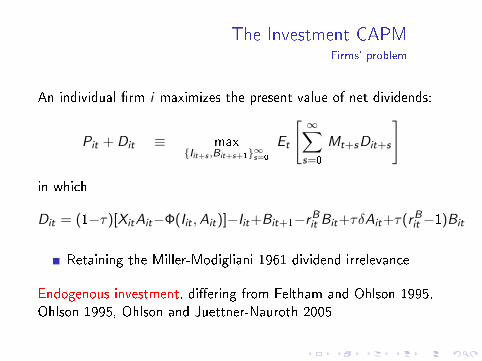
The Investment CAPMFirms' problem
An individual �rm i maximizes the present value of net dividends:
Pit + Dit ≡ max{Iit+s ,Bit+s+1}∞s=0
Et
[ ∞∑s=0
Mt+sDit+s
]
in which
Dit = (1−τ)[XitAit−Φ(Iit ,Ait)]−Iit+Bit+1−rBit Bit+τδAit+τ(rBit −1)Bit
Retaining the Miller-Modigliani 1961 dividend irrelevance
Endogenous investment, di�ering from Feltham and Ohlson 1995,Ohlson 1995, Ohlson and Juettner-Nauroth 2005

The Investment CAPMOptimal investment
The �rst principle of investment, Et [Mt+1rIit+1
] = 1, in which:
r Iit+1 =
(1− τ)
[Xit+1 + a
2
(Iit+1Ait+1
)2]+ τδ + (1− δ)
[1 + (1− τ)a
(Iit+1Ait+1
)]1 + (1− τ)a
(IitAit
)
The weighted average cost of capital (Modigliani-Miller 1958Propositions II and III):
r Iit+1 = wit rBait+1 + (1− wit) r
Sit+1
wit market leverage, rBait+1after-tax cost of debt

The Investment CAPMAn asset pricing theory derived from the supply of risky assets
Combining the neoclassical investment theory and Modigliani andMiller 1958 yields an asset pricing theory:
rSit+1 = r Iit+1 +wit
1− wit
(r Iit+1 − rBait+1
)
Complementarity: The consumption CAPM derived from thedemand of risky assets, the investment CAPM from supply
Both hold in equilibrium, delivering identical expected returns
Immune to the aggregation problem, the investment CAPM ismore empirically tractable than the consumption CAPM

The Investment CAPMImplications for fundamental analysis
Cross-sectionally varying expected stock returns:Investment-to-assets, expected pro�tability, and expectedinvestment growth
Security analysis in corporate bonds:
rBait+1 = r Iit+1 −1− wit
wit
(rSit+1 − r Iit+1
)
Fundamental analysis is consistent with e�cient markets:
Realized returns = expected returns + abnormal returns

Outline
1 Security Analysis: Background
2 The Investment CAPM
3 Comparison with Accounting Models
4 The Expected Growth Factor

Comparison with Accounting ModelsOverview
The investment CAPM has more appealing properties thanworkhorse accounting models

Comparison with Accounting ModelsThe residual income model
Preinreich 1938, Miller and Modigliani 1961, Ohlson 1995:
Pit
Beit=
∑∞τ=1
E [Yit+τ −4Beit+τ ]/(1 + ri )τ
BeitPit
Beit=
∑∞τ=1
E [Yit+τ − riBeit+τ ]/(1 + ri )τ
Beit

Comparison with Accounting ModelsFrankel and Lee (1998): The intrinsic-to-market value anomaly
Historical Roe- and analysts' forecasts-based intrinsic values:
V ht = Bet +
(Et [Roet+1]− r)
(1 + r)Bet +
(Et [Roet+2]− r)
(1 + r)rBet+1
V ft = Bet +
(Et [Roet+1]− r)
(1 + r)Bet +
(Et [Roet+2]− r)
(1 + r)2Bet+1
+(Et [Roet+3]− r)
(1 + r)2rBet+2
In the investment CAPM, true V equals P , but V h/P and V f /P asnonlinear functions of investment, pro�tability, and expected growth
Empirically, investment-to-assets absorbs V h/P and V f /P

Comparison with Accounting ModelsApplication of the residual income model for the cost of capital
A voluminous implied cost of capital literature:
Claus and Thomas 2001, Gebhardt, Lee, and Swaminathan2001, Easton 2004
Botosan 1997, Botosan and Plumlee 2002, Hribar and Jenkins2004, Hail and Leuz 2006, Pastor, Sinha, and Swaminathan2008, Lee, Ng, and Swaminathan 2009
Alas, the implied cost of capital (as the internal rate of return)does not forecast returns
Easton and Monahan 2005, Guay, Kothari, and Shu 2011
The one-period-ahead expected return from the investment CAPM

Comparison with Accounting ModelsTwo valuation functions from the investment CAPM
Marginal q equals average q (Hayashi 1982):
Pit =
[1 + (1− τ)a
(IitAit
)]Ait+1 − Bit+1
A new valuation function:
Pit =
(1− τ)
[Xit+1 + a
2
(Iit+1Ait+1
)2]Ait+1
+τδAit+1 + (1− δ)[1 + (1− τ)a
(Iit+1Ait+1
)]Ait+1
wit rBait+1+ (1− wit) rSit+1
− Bit+1
The value-pro�tability relation is convex

Comparison with Accounting ModelsThe Penman-Reggiani-Richardson-Tuna (PRRT, 2017) model
Building on Easton, Harris, and Ohlson 1992, PRRT work with:
Et [rSit+1] = Et
[Pit+1 + Dit+1 − Pit
Pit
]=
Et [Yit+1]
Pit+ Et
[(Pit+1 − Beit+1)− (Pit − Beit)
Pit
]
The expected change in the market-minus-book equity linked to theexpected earnings growth (Shro� 1995)

Comparison with Accounting ModelsScenarios
Mark-to-market:
Pit = Beit ⇒ Et [rSit+1] =
Et [Yit+1]
Pit
No earnings growth:
Pit+1 − Beit+1 = Pit − Beit ⇒ Et [rSit+1] =
Et [Yit+1]
Pit
Growth related to risk and return:
Ohlson and Juettner-Nauroth 2005: The expected return as aweighted average of the forward earnings yield andbook-to-market (a proxy for the expected earnings growth)

Comparison with Accounting ModelsRelated literature on the PRRT model
Penman and Zhang 2012: Accounting conservatism expenses R&Dand advertising, inducing high expected earnings growth
Penman and Reggiani 2013: Deferring earnings recognition raisesthe expected earnings growth, connected to risk (uncertainty)
Penman and Zhu 2014: Many anomaly variables forecast theforward earnings yield and two-year-ahead earnings growth in thecross section, in the same direction of forecasting returns
Penman and Zhu 2016: Regress future returns on variablesconnected to expected earnings growth to estimate costs of capital

Comparison with Accounting ModelsCommonalities with the investment CAPM
Both models study the one-period-ahead expected return, asopposed to the internal rate of return in the residual income model
The one-period-ahead expected earnings and expected growth asthe key drivers of the expected return:
Earnings scaled with the market equity in PRRT, but bookassets in the investment CAPM

Comparison with Accounting ModelsDi�erences from the investment CAPM
The PRRT model uses accounting insights to link the expectedmarket-minus-book equity change to the expected earnings growth
The investment CAPM uses the investment-value linkage tosubstitute, analytically, capital gain with investment growth
The PRRT model still has the market equity
The investment CAPM is more �fundamental� than the PRRTmodel

Comparison with Accounting ModelsDi�erences from the investment CAPM
The PRRT model picks earnings yield to proxy for the forwardearnings yield, and book-to-market to proxy for the expectedearnings growth to explain the cross section of expected returns
Investment-to-assets, pro�tability, and expected investment growthsubsume earnings yield and book-to-market empirically
Complementarity: Overlay the economics of the investment CAPMwith PRRT's accounting under uncertainty

Outline
1 Security Analysis: Background
2 The Investment CAPM
3 Comparison with Accounting Models
4 The Expected Growth Factor

The Expected Growth FactorMotivation
Prior work examines investment and pro�tability
Hou, Xue, and Zhang 2015, see also Fama and French 2015
But the expected growth e�ect unexplored
Although performing well, the q-factor model leaves 46 anomaliessigni�cant at the 5% level (Hou, Xue, and Zhang 2017)

The Expected Growth FactorRoadmap of empirical work
Construct cross-sectional forecasts of annual I/A changes
Form a factor based on the cross-sectional forecasts
Augmenting the q-factor model with the expected growth factor
Factor regressions with and without the expected growth factor

The Expected Growth FactorForecasting annual I/A changes
Annual Fama-MacBeth cross-sectional regressions of I/A changes
Motivating predictors based on a priori conceptual arguments:
Tobin's q: Erickson and Whited 2000
Cash �ow: Fazzari, Hubbard, and Petersen 1988
Total revenue minus cost of goods sold, minus selling, general, andadministrative expenses, plus research and developmentexpenditures, minus change in accounts receivable, minus change ininventory, minus change in prepaid expenses, plus change indeferred revenue, plus change in trade accounts payable, and pluschange in accrued expenses, all scaled by book assets (Ball,Gerakos, Linnainmaa, and Nikolaev 2016)

The Expected Growth FactorCross-sectional regressions of τ -year-ahead I/A changes,
weighted least squares, 1/1961�12/2016
OOS Correlationτ log(q) Cop R2(%) Pearson Spearman
1 Slope −0.03 0.55 4.78 0.15 0.19t −3.38 6.44
2 Slope −0.08 0.74 7.77 0.16 0.20t −5.55 6.25
3 Slope −0.09 0.76 7.77 0.17 0.21t −6.46 6.09

The Expected Growth FactorDeciles on expected I/A changes,
NYSE breakpoints with value-weights, 1/1967�12/2016
τ Low 2 3 4 5 6 7 8 9 High H−L
1 m 0.00 0.37 0.42 0.53 0.50 0.50 0.62 0.61 0.78 0.76 0.76tm −0.01 1.45 1.85 2.50 2.41 2.70 3.43 3.22 4.06 3.70 4.71
2 m −0.01 0.33 0.41 0.45 0.50 0.63 0.63 0.71 0.68 0.81 0.82tm −0.03 1.38 1.97 2.12 2.58 3.50 3.41 3.64 3.59 3.56 5.26
3 m 0.00 0.29 0.39 0.54 0.47 0.60 0.70 0.60 0.69 1.01 1.01tm −0.01 1.28 1.77 2.71 2.42 3.26 3.46 2.90 3.56 4.50 5.93
1 αq −0.35 −0.18 −0.16 −0.06 −0.18 0.00 0.10 0.07 0.29 0.44 0.78tq −3.43 −1.83 −1.36 −0.72 −2.33 −0.01 1.25 0.98 3.54 4.22 5.40
2 αq −0.29 −0.14 −0.20 −0.11 −0.08 0.01 0.01 0.10 0.29 0.52 0.82tq −2.96 −1.68 −2.69 −0.99 −1.10 0.14 0.18 1.31 3.33 4.03 5.03
3 αq −0.29 −0.10 −0.26 −0.14 −0.08 0.03 0.15 0.19 0.31 0.52 0.81tq −2.91 −1.18 −2.84 −1.72 −1.13 0.38 2.00 2.34 3.13 3.24 4.08

The Expected Growth FactorConstruction of the expected growth factor (2×3 sort with size),
factor spanning tests, 1/1967�12/2016
Mean α MKT Me I/A Roe R2
0.56 0.53 −0.16 −0.08 0.14 0.14 0.376.66 7.12 −8.13 −1.86 2.78 3.66
α MKT SMB HML UMD R2
0.58 −0.17 −0.12 0.07 0.10 0.388.75 −8.85 −3.56 2.22 5.88
α MKT SMB HML RMW CMA R2
0.56 −0.15 −0.09 −0.05 0.17 0.21 0.397.59 −7.36 −2.49 −0.91 2.65 3.68

The Expected Growth FactorThe Q5 model: MKT, Me, I/A, Roe, and Eg

The Expected Growth FactorUsing the Q5 model to explain 46 q-anomalies, 1/1967�12/2016
The Q5 model improves on the q-factor model substantially
H−L alpha m.a.e.
Magnitude #|t|≥1.96 #|t|≥3 Mean #pGRS<5%
q4 0.52 46 17 0.16 39Q5 0.34 19 4 0.12 18
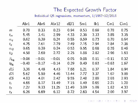
The Expected Growth FactorIndividual Q5 regressions, momentum, 1/1967�12/2016
Abr1 Abr6 Abr12 dEf1 Sm1 Ilr1 Cm1 Cim1
m 0.70 0.33 0.23 0.94 0.53 0.69 0.78 0.75
tm 5.45 3.41 2.99 4.33 2.36 3.33 3.85 3.35
αq 0.62 0.30 0.24 0.55 0.59 0.73 0.70 0.64
tq 4.25 2.61 2.79 2.49 2.15 2.94 2.84 2.36
αQ 0.65 0.30 0.24 0.53 0.55 0.68 0.76 0.46
tQ 4.58 2.60 2.72 2.25 1.88 2.82 2.96 1.63
βEg −0.06 −0.01 −0.01 0.05 0.08 0.11 −0.11 0.32
tEg −0.40 −0.17 −0.14 0.29 0.40 0.63 −0.63 1.67
d1i 3.36 4.48 4.43 7.68 1.21 0.37 1.84 0.94
d2i 5.67 5.50 4.46 13.44 2.77 3.37 1.62 3.09
d3i 4.83 4.01 2.47 9.55 2.48 2.89 2.03 2.93
t1 4.66 8.17 11.49 7.15 1.49 0.65 2.21 1.20
t2 7.27 9.33 11.25 11.49 3.09 5.09 1.82 4.33
t3 6.26 6.69 6.12 8.72 2.63 4.54 2.00 3.97

The Expected Growth FactorIndividual Q5 regressions, value-versus-growth, 1/1967�12/2016
Bmq12 Nop Emq1 Ocp
m 0.48 0.63 −0.71 0.70
tm 2.21 3.40 −3.21 3.14
αq 0.37 0.35 −0.48 0.36
tq 2.18 2.42 −2.00 1.98
αQ 0.38 0.08 −0.47 0.20
tQ 2.25 0.58 −1.92 1.14
βEg −0.03 0.49 −0.02 0.30
tEg −0.16 3.40 −0.09 1.67
d1i −7.70 18.44 0.30 −1.32d2i −5.16 24.26 −3.37 5.14
d3i −0.88 26.59 −4.98 7.70
t1 −6.97 13.59 0.36 −1.27t2 −4.00 13.66 −2.99 3.82
t3 −0.72 15.58 −5.79 6.43

The Expected Growth FactorIndividual Q5 regressions, investment, 1/1967�12/2016
Noa Nsi Cei Ivc Oa dWc dFin Dac Pda
m −0.44 −0.64 −0.57 −0.44 −0.27 −0.42 0.28 −0.39 −0.48tm −3.25 −4.46 −3.32 −3.33 −2.19 −3.25 2.39 −2.95 −3.91αq −0.45 −0.29 −0.29 −0.28 −0.56 −0.51 0.43 −0.67 −0.39tq −2.59 −2.32 −2.25 −2.08 −4.10 −3.80 3.00 −4.73 −2.60αQ −0.12 −0.12 0.00 −0.02 −0.26 −0.29 0.17 −0.32 −0.09tQ −0.79 −0.90 0.01 −0.13 −1.85 −2.16 1.22 −2.22 −0.61βEg −0.62 −0.33 −0.54 −0.49 −0.56 −0.41 0.49 −0.65 −0.56tEg −5.58 −3.14 −4.85 −5.47 −5.31 −3.50 5.61 −6.81 −5.57d1i −49.21 −34.29 −8.74 −30.09 −2.29 −16.25 36.33 −6.16 −3.21d2i −54.36 −39.42 −18.67 −35.02 −6.73 −21.13 36.28 −9.86 −8.07d3i −53.26 −40.18 −22.51 −38.45 −8.36 −21.03 37.35 −8.92 −10.02t1 −18.41 −14.71 −6.29 −24.94 −1.15 −12.18 19.42 −4.40 −1.77t2 −19.29 −16.68 −13.26 −28.37 −3.26 −14.17 18.31 −6.23 −5.53t3 −18.99 −16.49 −12.69 −26.66 −3.89 −12.56 18.42 −5.30 −7.15

The Expected Growth FactorIndividual Q5 regressions, pro�tability, 1/1967�12/2016
dRoe1 Atoq1 Atoq6 Atoq12 Opa Olaq1 Olaq12 Cop Cla Claq1 Claq6 Claq12
m 0.75 0.62 0.53 0.42 0.41 0.75 0.46 0.63 0.55 0.52 0.49 0.46tm 5.53 3.44 3.07 2.56 2.09 3.53 2.46 3.57 3.23 3.26 3.60 3.63αq 0.34 0.35 0.34 0.32 0.46 0.40 0.32 0.69 0.75 0.46 0.41 0.45tq 2.37 2.06 2.09 2.03 2.96 2.64 2.49 5.04 5.23 3.02 2.97 3.63αQ 0.42 0.07 0.09 0.09 −0.06 0.01 −0.10 0.12 0.19 0.09 0.01 0.07tQ 2.85 0.43 0.54 0.58 −0.42 0.06 −0.94 1.11 1.72 0.62 0.11 0.70
βEg −0.14 0.52 0.47 0.42 0.97 0.72 0.77 1.09 1.06 0.68 0.72 0.69tEg −1.09 3.79 4.13 3.99 10.19 7.22 9.46 14.53 13.88 6.53 9.90 10.65
d1i 5.02 6.83 7.83 7.31 10.88 11.50 6.47 20.49 7.33 −1.49 0.41 2.92d2i 14.38 11.37 10.10 7.98 12.22 12.98 5.76 27.01 12.58 6.40 6.93 7.43d3i 12.65 9.27 8.10 6.04 13.22 9.85 4.05 28.57 13.99 6.64 6.79 7.47t1 3.71 5.82 6.74 6.51 5.16 6.78 4.63 10.67 3.65 −1.85 0.59 4.12t2 17.09 7.87 7.69 6.81 4.75 6.94 3.93 12.73 7.05 7.77 8.48 8.50t3 15.38 6.22 5.94 5.00 4.83 4.94 2.47 11.99 7.18 7.04 7.38 8.12

The Expected Growth FactorIndividual Q5 regressions, intangibles, 1/1967�12/2016
Rdm Rdmq1 Rdmq6 Rdmq12 Rer Eprd R1a R
[2,5]a R
[6,10]a R
[11,15]a R
[16,20]a
m 0.70 1.11 0.80 0.82 0.34 −0.53 0.67 0.69 0.83 0.62 0.54tm 2.75 2.91 2.18 2.43 2.44 −2.96 3.43 4.11 5.06 4.46 3.26αq 0.72 1.39 0.95 0.81 0.34 −0.55 0.58 0.81 1.11 0.60 0.62tq 3.11 3.06 2.87 3.01 2.05 −3.02 2.75 4.06 5.05 3.48 3.22αQ 0.27 1.30 0.72 0.52 0.30 −0.48 0.52 0.79 1.00 0.57 0.57tQ 1.22 2.74 2.07 1.85 1.75 −2.97 2.47 3.82 4.78 3.40 2.64
βEg 0.86 0.17 0.42 0.52 0.08 −0.12 0.11 0.03 0.20 0.05 0.10tEg 5.12 0.50 1.35 2.18 0.49 −0.83 0.60 0.21 1.29 0.33 0.85
d1i −0.15 −6.05 −4.81 −2.54 −2.18 0.96 6.08 −2.58 −0.08 −0.94 0.40d2i 5.68 −3.05 0.47 4.65 4.30 1.56 4.32 −3.61 −1.12 0.08 0.51d3i 5.75 3.84 6.63 9.73 4.64 1.41 2.96 −5.15 −1.74 −0.69 0.85t1 −0.12 −2.86 −2.66 −1.84 −1.79 1.00 10.54 −4.33 −0.17 −1.81 0.98t2 3.11 −1.19 0.20 2.26 4.48 1.70 6.22 −6.51 −1.80 0.16 1.19t3 3.36 1.49 2.78 4.75 4.87 1.55 4.22 −8.52 −3.06 −1.21 1.84

The Expected Growth FactorIndividual Q5 regressions, trading frictions, 1/1967�12/2016
Is�1 Isq1
m 0.28 0.25
tm 3.11 2.80
αq 0.27 0.29
tq 2.56 2.84
αQ 0.23 0.19
tQ 2.02 1.74
βEg 0.09 0.19
tEg 1.13 2.39
d1i 0.10 0.35
d2i 0.17 0.81
d3i 0.23 0.72
t1 0.23 0.92
t2 0.39 1.63
t3 0.53 1.34

ConclusionThe economics of value investing
The investment CAPM reconciles the Graham-Dodd philosophy ofvalue investing with neoclassical economics
Cross-sectionally varying expected returns, depending on �rms'investment, pro�tability, and expected investment growth
An appealing alternative to accounting models forcharacterizing the cost of capital
An upgraded q-factor model augmented with an expectedinvestment growth factor (the Q5 model)