The Economic Impacts of Eminent Domain

Daniel L. Chen and Susan Yeh⇤

January 2012

Abstract

We model government takings of private property, embedding prominent theories

of their economic consequences. Random assignment of U.S. judges and the fact that

judges make takings precedent in a manner correlated with their race, political party,

and prior government advocacy facilitate causal estimates of allowing government

takings. Novel data on judicial biographies and takings decisions since 1975 indicate

that decisions favoring physical takings increase growth by 0.2% points but reduce

minority home ownership and employment by 0.5% and 0.3% points respectively,

while those favoring regulatory takings initially depress property prices but spur

economic growth in the medium-run by 0.7% points.

Keywords: Eminent Domain, Property Rights, Takings, Regulation, Growth, Inequality

JEL codes: R32, K11, R42, R52

⇤Daniel L. Chen, Assistant Professor of Law, Economics and Public Policy, Duke Law School,dchen@law.duke.edu; Susan Yeh, Sharswood Fellow in Law and Economics and Lecturer, Universityof Pennsylvania Law School, syeh1@law.upenn.edu. We thank Andres Sawicki for sharing data. Workon this project was conducted while Daniel Chen received financial support from the Ewing MarionKauffman Foundation. We acknowledge joint financial support from the John M. Olin Center for Law,Economics, and Business at Harvard Law School.

1

1 Introduction

The ability for governments to take land from individuals is hotly debated around the

world. In India and China, fatal riots have followed government acquisitions of private land

on behalf of commercial developers, while in the former Soviet bloc, legislation allowing

governments to take land for the establishment of privately-owned industrial parks is

pending.1 Referred to as eminent domain, compulsory purchase, compulsory acquisition,

or expropriation by different legal systems,2 a common question arises: is state taking

of private property justified? Proponents in the United States argue that government

exercise of eminent domain spurs economic growth through public goods provision, blight

removal, and commercial development (Kelo v. City of New London, 545 U.S. 469 (2005)).

Skeptics, however, believe that public choice incentives lead revenue-seeking governments

to collude with private developers (Byrne 2005) at the expense of disadvantaged groups

(see Justices O’Connor’s and Thomas’s dissents in Kelo) and believe that governments

compensate landowners too little for land acquisition (Chang 2010; Munch 1976). In the

U.S., contention surrounding government takings has risen to a new level: if governments

simply regulate and restricts certain property rights, such as the ability to use the land

productively, the regulation would be considered a taking.3 Liberty issues aside, little is

empirically known about the consequences of government takings, despite a plethora of

economic and legal theories regarding their potential consequences (Epstein (1985, 2008);

Kaplow 1986; Blume, Rubinfeld and Shapiro 1984).4

1See http://www.nytimes.com/2011/02/05/nyregion/05metjournal.html,

http://www.nytimes.com/2011/02/23/world/asia/23india.html, http://www.cga.ct.gov/2005/rpt/2005-r-0321.htm, and http://www.nytimes.com/2011/12/26/world/asia/in-china-the-wukan-revolt-could-be-a-harbinger.html?hp. In China alone, the government has taken land from an estimated 40million households, many of whom have been under-compensated and as a result remain landless andunemployed (Cao et al. 2008).

2Eminent domain (United States), compulsory purchase (United Kingdom, New Zealand, Ireland), re-sumption/compulsory acquisition (Australia), expropriation (South Africa and Canada).

3Pennsylvania Coal Co. v. Mahon (1922) established the doctrine of regulatory takings (see AppendixA). Examples of regulatory takings include zoning restrictions for the location of hotels (Dexter 345 Inc.

v. Cuomo, 2011 WL 6015780) and regulations shortening the fishing year (Vandevere v. Lloyd, 644 F.3d957).

4A growing literature in economic development links secure property rights (but not eminent domain) tohousing renovations (Field 2005), agricultural investments (Besley 1995), and agricultural productivity(Banerjee, Gertler and Ghatak 2002; Hornbeck 2010). An extensive theoretical literature in macroeco-nomics links economic growth to the ability by governments to expropriate capital (but not land) expost (Aguiar and Amador 2011).

2

Empirical studies to date have primarily focused on descriptive statistics. Data

limitations have made it practically impossible to study the causal effects of eminent

domain. Few centralized sources of data document the condemnation of property across

jurisdictions exist since various levels of government, local, state, and federal, are able to

invoke the power of eminent domain. We sidestep this issue by focusing on court-made

laws that make it harder or easier for subsequent government actors to take. We study

the U.S. because its common law system, random assignment of judges, and system of

appellate courts with regional jurisdiction setting legal precedent for millions of people,

allows us to isolate causal effects.

In particular, we derive a natural experiment from the random assignment of U.S.

appellate judges to three-judge panels exercising judicial discretion in interpreting the

facts and the law differently and in a manner correlated with their demographic char-

acteristics. Between 1979 and 2004, 220 federal appellate cases addressed regulatory

takings, and between 1975 and 2008, 134 appellate cases addressed physical takings. Our

empirical strategy exploits the fact that appellate decisions are binding precedent only

for future cases within the same circuit. Because judicial composition of eminent domain

panels is unlikely to be correlated with subsequent economic outcomes other than through

eminent domain decisions, the random assignment of judges creates exogenous variation

in appellate precedent making it harder or easier to exercise eminent domain. This ex-

ogenous variation can be used to estimate the causal impact of allowing eminent domain

on economic outcomes, since takings law can otherwise be endogenous to economic out-

comes. Among other channels, endogeneity arises because the Fifth Amendment of the

U.S. Constitution allows governments to take land only for “public use” and if there is

“just compensation.” For example, if property prices are expected to increase, then courts

may be less likely to rule that a condemnation or regulation meets the criteria for public

use such as blight removal or that the compensation is just. Thus appellate decisions fa-

voring private property rights would be endogenous to anticipated price trends, leading to

a spurious estimate were we to only examine the correlation between appellate decisions

and future property prices.

The sign of any effect of eminent domain on subsequent economic outcomes is

theoretically ambiguous. Section 2 embeds prominent theories of eminent domain in a

3

general model of both regulatory and physical takings, emphasizing how increased risk

of takings can distort incentives to develop land efficiently (Riddiough 1997) and, when

landowners receive full compensation for takings, overinvestment can occur because full

compensation provides full-coverage insurance to the private investor against the risk of

taking with no premium paid (Blume, Rubinfeld and Shapiro 1984; Miceli and Segerson

1994; Innes 1997; Turnbull 2002). After documenting that our model is consistent with

the predictions of models in the literature, we show how estimating the empirical impact

of eminent domain permits inference as to the predominant underlying mechanism, i.e.,

whether under- or over- investment or public use.

We present an analysis of zip-code level property prices, state GDP, home owner-

ship, and individual labor market outcomes as well as data on eminent domain appellate

decisions collected by ourselves as well as by other authors. Section 3 establishes that the

composition of judicial panels is indeed related to eminent domain appellate decisions.

After verifying that judges are effectively randomly assigned, we show that panels with

judges who are Republican appointees and prior U.S. Attorneys are more likely to uphold a

physical taking on behalf of the government while panels with judges who are Democratic

appointees and minority are more likely to rule against a physical taking. Republican ap-

pointees, who might generally favor commercial development as well as individual liberty

rights, might not have any particular stance on eminent domain on average, but those

who are prior U.S. Attorneys, a highly political and legal position, would have served on

behalf of the government and could view takings cases more favorably for the government.

A large literature, moreover, documents that black and white judges decide differently on

a range of issues (Chew and Kelley (2008); Scherer (2004); Kastellec (2011)), and minority

Democratic appointees are likely to have prior experiences serving people whose proper-

ties are physically taken, who tend to be poor and minority (Carpenter and Ross 2009;

Frieden and Sagalyn 1989). We show, in contrast, that panels with black (or minority)

judges are more likely to vote to uphold a regulatory taking against a plaintiff’s challenge,

as regulatory takings challenges tend to be brought forward by wealthier, non-minority

parties, especially business entities (Stein 1995).

A variety of evidence in Section 3 establishes that the random assignment of judges

differentially impacts appellate decisions creating legal precedent in eminent domain. In

4

Section 4, we consider the subsequent impact on property values, growth, and economic

inequality. Two-stage least squares estimates using this variation suggest that making

it easier to regulate without having to compensate landowners spur economic growth.

Property prices initially decline, but then increase in response to pro-takings regulatory

precedent. Making it easier to acquire private property increases growth in state GDP

and property prices, but decrease minority labor market outcomes. Our baseline estimates

indicate that rulings in favor of the government in regulatory takings cases spurs growth

in property prices by 0.2% points and growth in GDP by 0.7% points and ruling in

favor of the government in physical takings cases spurs growth in property prices by 0.12-

0.23% points and economic growth by 0.2% points. Significantly, however, pro-government

physical takings precedent reduces minority home ownership and employment by 0.5% and

0.3% points respectively. We verify our estimation strategy is robust to using alternative

judicial characteristics by implementing LASSO, a sparse model, to optimally extract

information from different combinations of judges on three-judge panels (Belloni et al.

2011). Our results provide evidence that the law of eminent domain has real economic

consequences.

In our analyses, we explore how closely our empirical design tracks a randomized

control trial by varying our controls and data in a variety of specifications. Previous

studies have not used randomization to address the issue of endogeneity of takings, where

property characteristics themselves, linked to the surrounding economy, can drive govern-

ment decisions that would in turn affect property values.5 The closest study preceding

ours is Guidry and Do (1998), which finds that property transferred under eminent do-

main correspond to higher property prices in a cross-sectional analysis of a small sample

of properties, and Quigley and Rosenthal (2005) conclude that as much as 54% of land

value can be linked to land use regulations.6 Methodologically motivated by Deaton

(2010) and Lee (2008), we show how the empirical framework developed here provides

causal estimates of court precedent holding all else equal including unobserved factors. It

overcomes the basic issues of omitted variables and reverse causality. Furthermore, it has5Cities are less likely to condemn occupied homes for economic redevelopment projects and are morelikely to take underutilized property (Mihaly (2006); Chang (2010)) in urban areas (Byrne 2005) andfrom minority and poor residents (Carpenter and Ross (2009)).

6Other studies have found increases in property values (Jaeger (2006); Katz and Rosen (1987); Beaton(1991)) though some find decreases (Nickerson and Lynch (2001)).

5

the advantages that the exclusion restriction is likely to hold, that the LATE interpreta-

tion of the IV estimates is policy relevant, that the general equilibrium effects are those

that we would want to include, and that the impulse response function is well-identified.

Our method should prove fruitful for policy-makers and judges interested in assessing the

impact of court-made law.

2 Background

This section outlines a theoretical model of government takings to guide our empirical

work. Appendix A develops the model formally. Physical takings and regulations are

decisions of the local, state, or federal government. Let ⇡p be the exogenous probability

that the court allows a physical taking to occur and the government must provide com-

pensation C > 0 and ⇡r be the probability that the court allows a regulation with zero

compensation C = 0.

Through stare decisis, the legal doctrine by which judges must respect the prece-

dents established by prior decisions, appellate court precedent increases or decreases these

probabilities, ceteris paribus, i.e., with the same fact patterns as found in previous takings

cases. Appendix B describes key elements of the U.S. legal context necessary for model

estimation and highlights major doctrinal developments. A pro-government decision in a

physical takings case lowers the threshold for what constitutes public use, so increases ⇡p.

A pro-government decision in a regulatory takings case raises the likelihood of subsequent

regulatory activity so increases ⇡r. With probability 1�⇡p�⇡r, the court rules in favor of

the plaintiff, and the government action is overturned. Compensation C depends only on

government policy and the property’s current condition. The landowner invests I in his

property to maximize expected returns, taking into account ⇡p and ⇡r, the government’s

probability of initiating a taking ⇡, compensation C, the government’s compensation

policy G (e.g., just or partial), and uncompensated losses L due to regulation:

max

IER = max

I{(1� ⇡)(V (I)� I) + ⇡[(1� ⇡p)V (I) + ⇡pC(G, I)� ⇡rL� I]} (1)

6

Our model shows that compensation is key to efficient investment in a world with takings.

The law requires the government to compensate the landowner in a taking, accounting

for a number of factors including the book value (appraisal price of the property). Under-

investment can arise if the government does not compensate property owners sufficiently.

Over-investment, however, can arise with just compensation because it removes the risk

that an investment could lose all value to the landowner when property is taken by the

government instead of sold at market value. Property owners are over-insured, or to put

it another way, do not pay the insurance premium on the insurance they receive in the

event of a taking (Blume, Rubinfeld and Shapiro (1984); Kaplow (1986)). Over-investment

results because the marginal increase in value to society is less than the marginal increase

in value to the individual. Our derivation in Appendix A provides a theory-based test for

the presence of under- or over-compensation. Translating to our empirical context:

• If there is under-compensation, then a higher probability of taking would lead to

lower investment and therefore lower property values, lower growth, and lower em-

ployment. This might occur particularly for minority landowners in physical takings

since their land is disproportionately condemned and under-compensated.

• If there is over-compensation, then a higher probability of taking would lead to

higher investment and therefore higher property values and higher employment but

lower growth in the medium or long-run (Green (2003)).

• If compensation is optimal, then the probabilities of taking should have no significant

impact on property values, growth, and unemployment.

We summarize:

Investment Level Growth/GDP vs.⇡p, ⇡r, ⇡

Employment vs.⇡p, ⇡r, ⇡

Property Valuevs. ⇡p, ⇡r, ⇡

Below first-best(Under-investment) - - -

At first-best(Optimalinvestment)

0 0 0

Above first-best(Over-investment) - + +

7

Social benefits from the public use project would be capitalized and directly impact

prices, growth, and employment, each of which we predict to be positively related to Br

and Bp. Making it easier for the government to take private property would stimulate

growth only if the social benefits, which may differ for regulatory and physical takings,

exceed the distortions from increased probability of taking when compensation is not

optimal.

3 Design of Study

3.1 Data

Our empirical analysis draws on several sources of data on eminent domain cases—established

datasets as well as our own data collection. Sunstein et al. (2006) collect data on all appel-

late regulatory takings published decisions from 1979-2004. We apply a similar method-

ology to collect appellate physical takings decisions from 1975-2008. We also collect all

district court cases involving regulatory and physical takings. Our outcome variables are

property values (house price indices) at the zip code level from the Fiserv Case-Shiller

Weiss data, state gross domestic product (GDP) from the Bureau of Economic Analy-

sis, and housing and employment outcomes from the Current Population Survey (CPS).

These and other data collection efforts are described further in Appendix C.

3.2 Specification

Our basic specification models the changes in eminent domain precedent at the circuit-

year level and its relationship to unit outcomes in those circuits over time:

Yict = �0 + �1Lawct + "ict (1)

The dependent variable, Yict, is a measure of outcomes of unit i in circuit c and time t. Our

main outcomes are change in log property prices at the zip code level measured at quarterly

frequency, change in log local GDP at the state level measured at yearly frequency, and

8

housing and employment status of individual i in circuit c at yearly frequency.7 The

key coefficient of interest is �1 on Lawct, where Lawct is the measure of eminent domain

precedent issued in circuit c and year t (or quarter t for property prices). Lawct is the

proportion of cases with a pro-government (pro-taking) outcome. In robustness checks,

we use the number of cases as weights.8

If eminent domain decisions and economic outcomes are systematically correlated

with omitted variables, then �1 is biased. For example, social trends may drive judi-

cial decisions, so ascertaining a causal effect from judicial decisions to social trends is

difficult. A particular form of endogeneity arises because the Fifth Amendment of the

U.S. Constitution allows governments to take land only for “public use” and if there is

“just compensation.” If property prices are expected to increase, then courts may be less

likely to rule that a condemnation or regulation meets the criteria for public use such as

blight removal or that the compensation is just. Thus appellate decisions favoring private

property rights would be endogenous to anticipated price trends, leading to a spurious

estimate were we to only examine the correlation between appellate decisions and future

property prices. An additional concern with judge-made law is that there is so much

cross-fertilization across different areas of legal doctrine (e.g. between tort and property

law). If different, but related, doctrinal areas have independent effects on economic out-

comes, social changes may be misattributed to one legal rule when many legal rules are

changing simultaneously.

The common approach of controlling for potential confounders can accentuate the

problem of omitted variable bias if the included terms are themselves correlated with

other omitted variables (Clarke (2005)):

Yict = �0 + �1Lawct + �2Cc + �3Tt + �4Cc ⇤ Time + �5Wct + �6Xict + "ict (2)7We also examine hours worked and log real weekly earnings. Earnings are normalized to account forinflation. We use CPS weights when examining labor market outcomes. Logs real weekly earnings aretaken of 1+earnings and earnings are set to 0 if an individual is not employed or not in the labor force.We do this because actual wages, not reservation wages, are of normative interest by legal scholars. Inrobustness checks, we also drop individuals not employed or not in the labor force.

8With less than one eminent domain decision per circuit per year, we did not consider quadratic ornon-monotonic functions of the number of pro-plaintiff decisions.

9

With a research design involving random treatment assignment, however, adding controls

can add precision to the estimates if the controls are strong predictors of the outcomes. We

show that our main estimates are invariant to the inclusion or exclusion of: circuit fixed

effects, Cc, and time fixed effects, Tt, to address whether fixed unobservable differences

within circuits and within time periods are correlated with pro-plaintiff precedent and

economic outcomes; circuit-specific time trends, Cc ⇤ Time, to allow different circuits to

be on different trajectories with respect to outcomes; state fixed effects to address the

possible influence of state-specific takings statutes or state interpretation of federal laws;

a vector of observable unit characteristics, Xict, depending on the unit being observed (for

example, at the individual level: age, gender, educational attainment, and race, which

each enter as dummies with the exception of age); and time-varying circuit-level controls,

Wct, such as the characteristics of the pool of judges available to be assigned.

Since economic outcomes are serially correlated, "ict is not i.i.d. Hence, all spec-

ifications cluster standard errors at the circuit level. Bester, Conley and Hansen (2011

forthcoming) suggest scaling up the cluster t-statistic with relatively few clusters (e.g.,

12 circuits), but the scaling is very close to one with large N. Barrios et al. (2010) in-

dicates that the use of clustered standard errors, along with the random assignment of

treatment, address possible spatial correlation in the errors as well. In robustness checks,

we also execute a wild bootstrap suggested by Cameron, Miller and Gelbach (2008) for

small number of clusters and a Monte Carlo simulation, where we randomly assign the

legal variation to another circuit to test for spurious correlations.

Since Lawct and "ict may be correlated due to uncontrolled-for social trends or other

legal developments that correlate both with Lawct and outcomes Yict, �1 may be biased.

To overcome this, we need an instrumental variable for Lawct that is uncorrelated with

"ict. Figure 3 roughly depicts the intuition for our 2SLS identification strategy, in which

we exploit the random variation that arises from using the random deviation in the actual

number of black judges per seat in eminent domain cases.9 These numbers are depicted in

jagged red lines in Figure 3 for each of the 12 Circuits. The smoother blue lines indicate

the expected number of judges with particular biographic characteristics per seat for each9Without loss of generality, we only write black judges and regulatory takings cases until we discuss thefirst stage analyses.

10

Circuit. Circuit-years receiving an unexpectedly high proportion of black judges on their

regulatory takings panels receive an unexpectedly higher proportion of pro-government

eminent domain decisions. Each spike in the actual number of black judges per seat above

the expected number of black judges per seat corresponds to the circuit-year randomly

receiving a “treatment” of more pro-government regulatory takings precedent. Thus,

changes in outcomes can be attributed to the “treatment” of pro-government eminent

domain precedent and not to other unobserved social trends or legal developments.

Figure 3 suggests the first stage equation:

Lawct = �0 + �1Treatmentct + �2Cc + �3Tt + �4Cc ⇤ Y ear + �5Xict + �6Wct + "ict (3)

where Lawct is defined as the percentage of decisions that are pro-government (pro-taking),

conditional on there being any decision in that circuit and time period. The “Treat-

ment” group (Treatmentct = 1) comprises people who experience an unexpectedly higher

percentage of pro-government decisions due to an unexpectedly higher actual number

of black judges being assigned to the regulatory takings panels. The “Control” group

(Treatmentct = 0) comprises people who experience an unexpectedly lower percentage

of pro-government decisions. Formally, Treatmentct = 1[(Nct/Mct > E(Nct/Mct)], where

Nct is the number of black judges assigned to all regulatory takings cases in that circuit-

quarter divided by 3 and Mct is the number of eminent domain cases in that circuit quarter.

The actual number of black judges per seat is given by Nct/Mct, while E(Nct/Mct) is the

expected number of black judges per seat. The moment condition for causal inference is

E(Treatmentct"ict) = E[1[(Nct/Mct�E(Nct/Mct))]"ict] = 0, which holds since being above

or below the threshold is uncorrelated with social trends or legal developments that might

otherwise be correlated with outcomes through ict. The effect of law on outcomes is the

difference in Outcomeict for Treatmentct = 1 or 0, divided by the difference in Lawct for

Treatmentct = 1 or 0. That is, we could simply look at the Wald estimator for outcomes

in any given year during or after the treatment to estimate the treatment effect.10 An10Note that economic outcomes are unlikely to zigzag in the manner suggested by the Figure 3. Rather,

we look for deviations from an underlying trend. Estimates of the treatment effect would be obtainedfrom differencing the average of these deviations for treated circuit-years with the average of thesedeviations for non-treated circuit-years.

11

illustration of such a calculation is displayed in Appendix Table A17.11

Before moving on to extensions of the basic model, we make two remarks. First,

the exclusion restriction is likely to hold, and we will thus be able to interpret the 2SLS

estimates as the causal impact of eminent domain precedent. Here, the identity of judges

sitting on eminent domain panels is not likely directly to affect economy-wide outcomes

that are of interest except through the appellate precedent alone.12 Second, the LATE

interpretation of the instrumental variables estimate is restricted in terms of external

validity. Here, only cases where there is enough controversy to allow judicial biographical

characteristics to matter are going to be the subject of the study. These cases may very

well be the difficult decisions that set new precedent, and the sorts of cases in which

judges interested in empirical consequences of decisions, like Judge Richard Posner or

Justice Stephen Breyer seek guidance (Posner (1998); Breyer (2004)).

For more statistical power, we employ the entire excess proportion of black judges

per seat as a continuous instrumental variable. That is, we write:

Lawct = �0 + �1Zct + �2Cc + �3Tt + �4Cc ⇤ Time + �5Wct + �6Xict + "ict (4)

where Zct is the difference between the actual number of black judges per seat and the

expected number of black judges per seat. The moment condition for causal inference

is E[(Nct/Mct � E(Nct/Mct))"ict] = 0. In words, the greater the excess proportion of

black judges per case, the more pro-takings is the regulatory takings precedent in that

circuit-year. We attribute the degree to which outcomes change to this excess proportion.

Laws are not likely to have an immediate impact. Firms may need time to adjust

to judicial decisions; alternatively, the effects of a law change may fade as expectations or

statutory regimes adjust. We build on our basic model with a distributed lag specification11The ratio of the differences is comparable to the point estimates displayed in Table 5 Panel A and

Appendix Table A10.12Causation from demographic characteristics to decision-making is not necessary for the methodology.

Rather, only correlation is needed. The exact mechanism for why demographic characteristics affectdecision-making is also irrelevant. For example, decisions could be different because litigants tailortheir oral arguments to the judge. We use demographic characteristics instead of judicial attitudesbecause demographic characteristics provide a multivariate characterization of judges that can be usedacross judges. These characteristics provide additional power relative to attitudinal scores, which areunidimensional, or to individual judge fixed effects, which would be imprecisely estimated if each judgehears only a handful of eminent domain cases.

12

that includes four years (16 quarters) of lags of the law and a one year (4 quarters) lead.

The use of leads helps assess whether trends in property prices precipitate eminent domain

precedent.13 We therefore estimate a distributed lag specification to study the dynamic

effects of law over time:

Outcomeict = �0 + �1y

XLawc(t�y) + �2Cc + �3Tt + �4Cc ⇤ Time (5)

+�5y

XWc(t�y) + �6Xict + "ict

A problem with this dynamic treatment effect specification is that circuit-years

with no cases greatly reduce sample size. If no appellate cases appear in any of the last,

say, 16 quarters, the observation would drop from the estimation. To address this missing

data problem, consider the moment condition for causal inference:

E[(Nct/Mct � E(Nct/Mct))"ict] = 0 (6)

We seek to construct an instrumental variable whose moment conditions will imply the

original moment condition. Consider an instrument, pct �E(pct). The moment condition

for this instrumental variable is:

E[(pct � E(pct))"ict] (7)

where pct is the number of black judges per seat in regulatory takings cases in circuit c

and time t and pct is defined as 0 when there are no cases. Specifically, let:

pct =

8><

>:

Nct/Mct if 1[Mct > 0]= 1

0 if 1[Mct > 0]= 0

(8)

and define Lawct also as 0 when there are no cases. When 1[Mct > 0] = 1, pct = Nct/Mct

returns the original moment condition E[(Nct/Mct�E(Nct/Mct))"ict] = 0. When 1[Mct >

13This test subsumes the standard check for a reduced form relationship between the instrument and theleads. Such a relationship would be included in the second-stage estimates of the lead coefficient sincethe first stage for the lead law includes all the instruments, leads and lags.

13

0] = 0, then pct = 0 and E(pct) = 0, so E[(pct � E(pct))"ict] = 0. However, these two

conditional moment conditions do not imply E[(pct � E(pct))"ict] = 0 unconditionally.

The presence of appellate cases, 1[Mct > 0], may be a function of "ict, so it needs to be

controlled. After controlling for it, then E[(pct � E(pct))"ict] = 0 unconditionally.

In addition, since E[(pct � E(pct))"ict] = E(pct"ict) � E[E(pct)"ict] = E(pct"ict) �

E(pct)E("ict) = E[pct"ict], we can ignore E(pct), the expected number of black judges per

seat. We have now constructed our instrumental variable, pct. This allows a distributed lag

specification since there is no dividing by 0, but one needs to include a binary indicator

1[Mct > 0] representing whether there are cases. This binary indicator ensures that

circuit-years with no black judges assigned to cases are treated differently if there are no

appealed cases in that circuit-year.

The inclusion of 1[Mct > 0], however, threatens the moment condition in a dis-

tributed lag specification. Whether there are any cases in a given year may respond to

previous years’ realization of the instrument. That is, having many black judges being as-

signed to regulatory takings cases in prior years may affect litigants’ willingness to appeal

in the current year. If this is the case, then treatment affects both the left and right-hand

side and leads to downward bias in the estimates of interest with the greatest downward

bias in the most lagged treatment and the least downward bias in the least lagged treat-

ment (such as lead coefficients). This form of downward bias makes the distributed lag

specification difficult to interpret.

To address this potential downward bias, we instrument for 1[Mct > 0] with the

random assignment of district court judges to their cases. One district court judge is ran-

domly assigned per case (Bird (1975)).14 Figure 1 displays the boundaries of each district

court with dashed lines. Whether the district court cases were disproportionately assigned

to certain types of judges will be uncorrelated with treatment (the random assignment

of appellate judges) but may affect the likelihood of subsequent appeal. Theoretically,

district judges could affect the likelihood of appeal, for example, if some district judges

are less likely to be reversed and this lower reversal rate discourages litigating parties from

pursuing an appeal. Indeed, the correlation between district judge demographic character-14We use only cases decided by district court judges and exclude recommendations by magistrate judges

because litigants cannot directly appeal a magistrate judge’s recommendation (28 U.S.C. § 636(c)(1)).

14

istics and their reversal rates has been documented (Steinbuch (2009), Barondes (2011),

Haire, Songer and Lindquist (2003), Sen (2011)). Once we identify both 1[Mct > 0] and

Lawct , then the number of lags and leads in our model will not matter since additional

lags and leads of our fitted 1[Mct > 0] and Lawct would be orthgonal to other years’ fitted

1[Mct > 0] and Lawct.15

Eminent domain appellate decisions affirm or overturn a local regulation or con-

demnation that potentially affects a large portion of the circuit since some regulations

are at the state level. To distinguish between the geographically local direct effects and

the precedential effects of an appellate decision, we coded the corresponding zip codes

for the regulation or condemnation addressed in each case in our database (see Appendix

Figures A1). In robustness checks, we estimate the specification Yict = �0 + �1Lawct +

�2LocalLawict + "ict, where we separately instrument for Lawct and LocalLawict using

the random assignment of judges in cases that occur in the zip code locally and in cases

that occur in the circuit. We apply this specification to property price data only since

our other datasets are not available at the zip code level and conduct our analysis at the

circuit-quarter level using the calendar month of each decision. In principle, analysis at

the circuit-quarter level would increase the number of experiments by fourfold relative to

analysis at the circuit-year level.

3.3 Interpretation

It is important to note the difference between the conditional and unconditional effect of

Lawct. The conditional effect is the one of policy-interest to a judge making a decision on

a case already in front of him or her. The counterfactual for a pro-government decision

is a pro-plaintiff decision. The unconditional effect is the one of policy-interest to an

advocate or historian interested in the social change that is due to court-made law. The

counterfactual for a pro-government decision is no decision. For example, to calculate

the effect of 1 pro-government decision when there is only 1 decision in that circuit-year,

we would need to add the effect of 1[Mct > 0] with the effect of Lawct to obtain the15The results could, of course, vary depending on the observations that need to be dropped to allow for

additional years of lags or leads, the need to fit additional parameters, and the coarsening of the firststage because all lags and leads of all instruments are used for any given endogenous variable.

15

unconditional estimates of going from 0 to 1 pro-government decision.16 We show the

distributed lag coefficients for conditional effects of Lawct. We also show the average lag

coefficients of Lawct and of 1[Mct > 0], their respective joint tests of significance, and

joint tests of significance for the distributed lags of Lawct+1[Mct > 0].

In interpreting the magnitudes, we discuss the “typical ” conditional (unconditional)

effects, which refers to the causal effect of the typical number of pro-government takings

appellate decisions in a circuit-year. For example, to get the typical conditional effect,

we multiply the conditional effect of Lawct by E[Lawct|1[Mct > 0]], the typical propor-

tion of decisions that are pro-government when there are appellate takings cases, and by

E[1[Mct > 0]], the proportion of circuit-years with an appellate takings case.17 For uncon-

ditional effects, we calculate the typical effect of pro-government decisions, pro-plaintiff

decisions, and all decisions. These are, in turn: 1[Mct > 0]*E[1[Progovernmentct >

0]]+Lawct*E[Lawct|1[Mct > 0]]*E[1[Mct > 0]], 1[Mct > 0]*E[1[Proplaintiffct > 0]], and

1[Mct > 0]*E[1[Mct > 0]]+Lawct*E[Lawct|1[Mct > 0]]*E[1[Mct > 0]].18 All of these

calculations could be multipled by four to obtain cumulative effects.

3.4 First Stage

We begin our analysis by examining whether different outcomes result from eminent

domain cases being assigned to judges with different background characteristics. The

only prior study of this question documents that political affiliation alone does not predict

decisions in eminent domain cases Sunstein et al. (2006). This lack of correlation with

political affilation, which we confirm, may be due to Republican appointees being both

pro-growth and pro-individual property rights relative to Democratic appointees. Instead,

we find that Republican appointees who are prior U.S. Attorneys are more likely to vote

pro-government, but minority Democratic appointees are more likely to vote pro-plaintiff

in physical takings cases, and black (and minority) judges are more likely to vote pro-16To calculate the effect of n pro-government decisions when there are m decisions, we would need to add

1[Mct > 0]+n/m*Lawct.17Both E[Lawct|1[Mct > 0]] and E[1[Mct > 0]] are displayed in Table 1.18The effect of 1 pro-government decision in a typical circuit-year is 1[Mct > 0]+Lawct/E[Mct|1[Mct >

0]]. E[Mct|1[Mct > 0]] is obtained from dividing E[Mct], the typical number of appellate takingspanels, by E[1[Mct > 0]], the proportion of circuit-years with an appellate takings case. Both E[Mct]and E[1[Mct > 0]] are displayed in Table 1.

16

government in regulatory takings cases.

These voting patterns are intuitive, given the highly political nature of U.S. At-

torney positions. U.S. Attorneys, who are appointed by the President, hold discretion

in prosecuting particular types of crimes, and their political orientation can wield a sub-

stantial influence (Lochner (2002); Perry (1998)). Partisan bias, for example, has been

documented in the prosecution of federal public corruption cases (Gordon (2009)). Re-

publican appointees who are prior U.S. Attorneys would have advocated on behalf of

the government and may be less likely to support the pro-individual property rights di-

mension of the Republican platform while retaining the pro-economic growth aspect of

the party priorities. Republican-prior U.S. Attorneys also vote in favor of the govern-

ment in regulatory takings cases, though less significantly so, perhaps because business

entities constitute the largest share of regulatory takings plaintiffs and Republicans have

traditionally been pro-business.

In contrast, that minority Democratic appointees tend to favor the plaintiffin

physical takings cases may relate to the phenomena that people whose properties are

physically condemned tend to be poor and minority (Carpenter and Ross (2009); Frieden

and Sagalyn (1989)). Minority Democratic appointees may have prior experience serving

on behalf this demographic, or they may consciously or unconsciously sympathize based

on their backgrounds. Minority Republican appointees, however, vote in favor of the

government in physical takings cases. Notably, many of these judges previously served

in U.S. Attorneys General offices. Indeed, prior research has documented that prior

experiences may make judges more susceptible to priming of group identity (Berdejo

and Chen (2010)).19 Along these lines, black judges may be more likely to favor the

government in regulatory takings challenges, because such regulatory takings challenges

tend to be brought forth by relatively wealthy, non-black individuals, with business entities

constituting the largest share of regulatory takings plaintiffs (Stein (1995)). Most notably,

black judges have been found to vote differently than white judges on affirmative action,

race harassment, unions, and search and seizure cases in a manner consistent with the

interests of their group identity (Chew and Kelley (2008); Kastellec (2011); Scherer (2004);19Asmussen 2011 and other scholarship also suggest that Presidents who appoint minority candidates

take the opportunity to appoint more ideologically extreme individuals than they would otherwise.

17

Brudney et al. (1999)).

Table 2 shows that black judges are 11% more likely to vote in favor of the govern-

ment (pro-takings) in regulatory takings cases (Panel A).20 At the case level, an additional

actual black judge per seat on a three-judge panel increases the chances of a pro-takings

decision by 33% (Panel B). At both the judge level and case level, point estimates and

statistical significance increase with controls for circuit and year fixed effects and the ex-

pected judge type per seat. At the circuit-year level, an additional actual21 black judge

per seat increases the proportion of pro-government regulatory takings decisions by 40%

(Panel C). These estimates are slightly different from the case level since cases are not

evenly distributed across circuit-years.22 The estimates and statistical significance are

robust regardless of whether the circuit-years with no cases are dropped or are dummied

and the proportion of pro-takings decisions and judge type per seat are set to 0 for those

circuit-years with no cases.23 The F-statistic is 6.9 and increases with the inclusion of

controls up to 26.6. The R-square does not change much with the inclusion of these

controls. The first stage analysis is similar for the circuit-quarter level (Panel D).

At the level of our analysis, merged with price data, the estimates are slighly

different because of the differing numbers of zip codes per circuit (Panel E). The joint

F statistic on the two instruments is well past the conventional threshold for weak in-

struments at 15.9 (Stock and Yogo (2005)), and the F statistics again increase with the

inclusion of fixed effects and additional circuit-year controls up to 17. A falsification of

the instrumental variables shows that this kind of legal variation is not related to the

instrument in the one or two years before and after the true instrument (Appendix Table

A2).

To check whether our (linear) specifications miss important aspects of the data,20All analyses in this section cluster standard errors at the circuit level.21In what follows, when the term is omitted, we always mean actual as opposed to expected.22Not every circuit-year has a case and cases can bunch up unevenly across circuit-years. For an example

of how a coefficient can differ between circuit-year and case level, suppose there are 4 cases, one caseeach with 0, 1, 2, or 3 judges who are black, and suppose that the panel makes a pro-governmentdecision when there are 3 black judges. If 1 circuit-year has the case with 0 black judges and the othercircuit-year has the remaining 3 cases, the coefficient at the circuit-year level is 0.5 (= difference inpercent pro-takings/difference in black judges assigned per seat) but when the 1 circuit-year with thecase has the case with 1 black judge, the coefficient at the circuit-level is 1.5. This example also showshow an increase in the probability of a pro-government decision due to an additional judge of a typeper seat can be greater than 1.

23The R-square increases significantly.

18

Figure 4A presents nonparametric local polynomial estimates of the effect of number of

black judges per seat on the proportion of pro-government decisions.24 The relationship

is monotonically increasing and not driven by outliers. In other words, having randomly

more black judges assigned corresponds to unexpectedly more pro-government takings

decisions. Similar results obtain with minority judges.

We conduct an identical analysis for physical takings in Table 3. Minority Demo-

cratic appointees are 20% less likely to vote in favor of the government in physical takings

cases while Republican appointees who are prior U.S. Attorneys are 18% more likely to

vote in favor of the government (Panel A). Similar patterns hold at the case level (Panel

B). At the circuit-year level, an additional minority Democratic appointee reduces the

proportion of pro-takings decisions by 62%, while an additional Republican-prior U.S.

Attorney judge per seat increases the proportion of pro-takings decisions by 93% (Panel

C).25 The joint F-statistic is 9 and increases with the inclusion of controls up to 19. The

first stage analysis is similar for the circuit-quarter level and the F-statistic ranges from

12 to 13. At the level of our analysis, merged with price data, the joint F statistic on

the two instruments exceeds the conventional threshold for weak instruments at 43 (Panel

E). Nonparametric local polynomial estimates show that the relationship is monotonically

increasing between Republican-U.S. Attorney judges and pro-government decisions while

it is decreasing, though less sharply so, for minority Democratic appointee judges and

pro-government decisions (Figure 4B). Neither relationship is driven by outliers.

3.5 LASSO Instruments

Some econometricians recommend larger first stage F-statistics to ensure that the first

stage is sufficiently strong, such as F stat=25 or 50 to allow for heteroskedasticity and

serial autocorrelation (Olea and Pflueger (2010)) The number of possible combinations of

judges or demographic characteristics on a judicial panel is very large, because judicial24Estimation proceeds in two steps. In the first step, we regress the proportion pro-government on circuit

and year fixed effects and we regress the number of black judges per seat on the same. Next, we takethe residuals from these two regressions and use the nonparametric local polynomial estimator to char-acterize the relationship between black judges and pro-government decisions. We use an Epanechnikovkernel with the default bandwidths selected by Stata.

25Such large point estimates are possible if having 1 Republican-prior U.S. Attorney tips the decision andthere are few cases with 2 Republican-prior U.S. Attorneys.

19

demographics are heterogeneous within each circuit and a circuit may have as many as

forty judges in the pool of judges available to be assigned. With this very large number of

possible panel compositions, our strategy benefits from a surfeit of experimental variation.

Choosing among a large number of instruments, however, is a challenging statistical issue

involving a trade-off between increasing the power of the first stage regression (Angrist and

Imbens (1995)) and avoiding the weak instruments problem with additional instruments

(Stock and Yogo (2005).

We use a LASSO technique to address this issue of instrument selection (Belloni et

al. (2011)) and to verify the robustness of our main IV results to alternative instruments.

Using LASSO (least absolute shrinkage and selection operator) in the first stage presents

several advantages relative to using OLS. While OLS has low bias, it also has two disad-

vantages. First, OLS lacks sparseness: large subsets of covariates are deemed important,

resulting in too many instruments, which makes 2SLS susceptible to a weak instruments

problem. Second, OLS lacks continuity: changing the data a bit results in different sub-

sets of covariates deemed important. LASSO is a sparse model, which solves both of these

problems. Formally, LASSO modifies OLS by minimizing the sum of squares subject to

the sum of the absolute value of the coefficients being less than a constant. The nature

of this constraint tends to set some coefficients to exactly 0 and hence reduces model

complexity. Intuitively, LASSO gives interpretable models by imposing a data penalty

for having too many covariates. In addition, LASSO ensures stability in instrument selec-

tion, making it an effective tool in selecting optimal instrumentals from a large number of

valid instruments. Belloni et al. (2011) show that LASSO is theoretically optimal under

certain conditions including sparsity.26 Because it selects optimal instruments, LASSO

enhances statistical precision when using the random assignment of judges.27 Intuitively,

optimal instruments are the strongest predictors of the endogenous variable where the

cross-correlation of the predictors are such that the two-stage least squares maximizes the

amount of information that can be obtained from exogenous predictors of the endogenous

variable. On a separate note, the use of the LASSO instruments provides a check of over-26Even if sparsity were not satisfied, LASSO can still be effective for finding relevant instrumental vari-

ables.27Belloni et al. (2011) show that the increased uncertainty due to selecting among many instruments

does not show up to first order.

20

identification since the two-stage least squares estimates derived from different judicial

characteristics should be similar assuming homogenous treatment effects.28

To construct our potential LASSO instruments, we use 30 biographical character-

istics29 and their interactions at the judge level and panel level,30 yielding a total of 900

possible instruments. The instruments chosen by the LASSO procedure are listed in Ap-

pendix Table A3. For example, at the circuit-year level, the LASSO procedure selected

Democrat prior assistant U.S. Attorneys for regulatory takings. The F statistic is 38,

representing a 100% improvement over the non-LASSO first stage F-statistics displayed

in Column 5 of Panel C in Tables 2 and 3. We consider a similar set of biographical

characteristics and instrumental variables for the district judges to identify an exogenous

component of the existence of an appeal. The random assignment at the district level is

not correlated with the random assignment at the appellate level. In our main tables, we

show the two-stage least squares results using the district LASSO instruments.

4 The Impact of Eminent Domain

4.1 Governmental and Market Response to Appellate Decisions

We should expect to see an effect if the following three assumptions are met: judges follow

precedent; on the margin, pro-takings decisions in appellate courts make it easier for

subsequent government actors to take; and market actors respond to appellate decisions.

While the first assumption is less contested, we examine the second two assumptions.

In separate analyses (Chen and Yeh 2011), we document that land appropriations for

transportation projects shift in response to eminent domain decisions. We use a dataset28By homogenous treatment effects, we mean the assumption that close cases whose decisions could be

affected by the judicial panel composition affect economic outcomes in the same manner regardless ofthe type of judicial panel.

29Democrat, male, male Democrat, female Republican, minority, black, Jewish, Catholic, No religion,Mainline Protestant, Evangelical, bachelor’s degree (BA) received from same state of appointment, BAfrom a public institution, JD from a public institution, having an LLM or SJD, elevated from districtcourt, decade of birth (1910s, 1920s, 1930s, 1940s, or 1950s), appointed when the President and Congressmajority were from the same party, ABA score, above median wealth, appointed by president from anopposing party, prior federal judiciary experience, prior law professor, prior government experience,previous assistant U.S. attorney, and previous U.S. attorney.

30For example, for the combination of “black and Democrat,” we examine the number of black Democraticappointees per seat for the judge level interactions and examine the number of Democrat appointeesper seat multiplied with the number of black judges per seat for panel level interactions.

21

provided by the Uniform Relocation Assistance and Real Property Acquisition Policies

Act of 1970, which requires states to report basic statistics about property transfers for

transportation projects. In response to pro-takings physical (but not regulatory) takings

cases, local governments become more likely to displace commercial landowners, who

are more expensive to relocate, even as compensation remains the same or falls. We

further document that the number of ordinances and exactions that become codified

also increases after pro-takings decisions. In other work, we show that markets, firms,

and media respond to appellate decisions. For example, media stock prices respond to

appellate decisions on FCC actions affecting media firms but not non-media firms (Chen,

Yeh and Araiza (2011)), the number of newspaper reports about the appellate topic

increase in response to appellate decisions in the circuits where the decisions occur (Chen

and Yeh (2011); Chen, Yeh and Araiza (2011)), and firms adopt sexual harassment human

resources policies subsequent to pro-plaintiff appellate sexual harassment decisions (Chen

and Sethi (2011)). We now turn to the effects of eminent domain decisions on property

prices.

4.2 Property Prices

4.2.1 Regulatory Takings

Pro-government decisions in appellate regulatory takings cases, which make it easier to

regulate without having to compensate landowners, spur growth in property prices. Table

4 Panel A shows the main results for the distributed lag specification of first-differenced

log house prices. Column 1 displays the naïve OLS estimates. The OLS lead coefficient

is the largest and statistically significant at the 1% level, indicating the importance of an

instrumental variables strategy to address trends that may drive both prices and judicial

decisions (Column 1). Indeed, in the IV estimates, the lead coefficient is not statistically

significant and its magnitude is a fraction of the magnitude of the lag coefficients (columns

2-9).

Column 2 displays the estimates using appellate-level IV, Column 3 displays the

estimates using both appellate and district-level IVs, Column 4 displays the estimates

using LASSO to select the appellate IV, and Column 5 uses LASSO for both appellate

22

and district IV. Columns 6-9 display the corresponding IV estimates when the data is

collapsed to the circuit-year level using population-weighted averages. Because change

in prices may be autocorrelated, it is customary to rely on joint tests of significance

to determine whether the effects are statistically significant. The main IV estimates in

Column 2 are not individually statistically significant, but they are jointly significant

at the 1% level. The average lag effect is 0.005, which indicates that a pro-government

regulatory takings decision (more precisely, when 100% of regulatory takings decisions

are pro-government instead of pro-plaintiff) increases property price growth by 0.5 log

points (percentage points) on average in each year for the next four years.31 When using

IV for both the appellate decisions and the presence of an appeal from the district court,

the average lag effect is similar in magnitude and the individual coefficients are similar

in magnitude and more statistically significant, though their joint significance weakens

(Column 3).32 Using LASSO instruments at the appellate level gives jointly significant

effects whose average is similar in magnitude to the previous estimates (Columns 4 and 5).

At the circuit-year level, the estimates are not significantly different from 0 when using

the non-LASSO instrument of black judges (Columns 6-7) but becomes more precisely

estimated and statistically significant when using the LASSO instrument (Columns 8-9).

The average effect is similar to the average effects found at the zip-year level in Columns

2-5.33 In unreported regressions, when we weight by the number of cases in the current

and previous 4 years to take into account the number,34 instead of percentage, of pro-

takings cases, the estimates become more statistically significant and precisely estimated

across the specifications.35

31The outcome is quarterly change in log prices. If the mean dependent variable of 1.1% is annualized,the average yearly change is about 5%, which is close to average local GDP growth displayed in Table5 and to annualized growth in other studies using the same data (Mian and Sufi (2009)).

32Estimates using the district IV may be less precise than the estimates without district IV becausethe LASSO-selected district IV have, at worse, F-statistics of around 8, just below the conventionalthreshold for strong instruments. Estimates may be further weakened because we greatly increase thenumber of endogenous variables to 12 and the number of instrumental variables to 36. While theoff-year (e.g. contemporaneous appellate instrument on lag pro-takings precedent) and off-level (e.g.district instrument on pro-takings precedent) instruments are statistically insignificant, the cumulationof off-year/off-level coefficients as illustrated in Appendix Table A2 may be an issue.

33The R-square is of less value in the IV context and is not reported in some of the IV regressions.34Both treating Lawct as an average of Mct number of decisions or as appearing with Mct frequency show

improvements.35In additional unreported results, the results change little when we control for lagged dependant vari-

ables, whether in levels or changes.

23

Appendix Table A4 presents a number of robustness checks using the main IV

specification in Table 4, Column 2 as the baseline. Columns 1-3 show the average of

the yearly lags, joint F test of the lags, and joint F test of the leads, respectively. The

robustness checks include: adding circuit-specific time trends (row A), removing circuit

and year fixed effects (row B), clustering standard errors at the state level, which exceeds

the conventional threshold for the number of clusters (row C), controlling for the expected

number of black judges per seat (row D), using zip code level population weights (row

E), and adding 2-year leads (row F). As randomization would predict, for each check, the

point estimates hardly change36 and the statistical significance generally increases with

the inclusion of controls, especially fixed effects. When we drop 1 circuit at a time, the

average lag estimates change little (row G), though the joint significance varies. Using

legal variation at the circuit-quarter (row I) reveals slightly larger point estimates and

statistical significance. The lead coefficients are typically insignificant.

Appendix Table A5 further verifies the robustness of our distributed lag specifi-

cation by showing the point estimates for each lag and by varying the number of lags

and leads. Consistent with the baseline IV results in Column 2 of Table 4, the point

estimates of the individual lags are insignificant. However, each row suggests a negative

initial impulse that is eventually overcome by a net positive response, as revealed by the

point estimates on the more distant lags (rows A-F) and by the robustness of this pattern

to varying the number of lags and leads (row G). Notably, in the specification with 4 leads

and 1 lag, none of the lead coefficients are individually or jointly statistically significant

and the magnitudes of the leads are an order of magnitude smaller than the estimated

lags. When controlling for the local direct effect of the taking, the precedential effects

become slightly larger (rows H-I). The local direct effects are opposite in sign. The lead

coefficients of the precedential effects are negligible while the lead coefficients of the local

direct effects are larger in absolute value than the lag coefficients of the local direct effects;

this pattern is consistent with the local taking having occurred quite a few years before

the appellate decision.37

36The point estimate becomes negative when using population weights, but Column 6 in Table 4 showsthat the impact on population-weighted mean outcomes is, in any event, not distinguishable from 0 andColumn 7 in Table 4 also shows an imprecisely negative impact. Moreover, when we use the LASSOinstrument in order to correspond to Column 8 in Table 4, the point estimate is positive and significant.

37The mean local direct takings effect on growth is still negative even accounting for the lead coefficients.

24

We also observe the pattern of having a negative impulse followed by net posi-

tive growth by years 3 and 4 when we use log price index as the outcome and include

circuit-specific time trends as the default specification in the same set of robustness checks

(Appendix Table A6).38 According to our model, negative price effects may be due to un-

derinvestment as with regulations, governments typically do not compensate landowners.

However, as we discuss later, the impact on economic growth is positive, suggesting that

the public use benefits eventually outweigh underinvestment.

Having established that our empirical framework approximates a randomized con-

trol trial, we next interpret the magnitude of our estimates. Conditional on the presence

of an appeal, the average effect of pro-takings precedent on property price growth is 0.5%

points (Column 2 of Table 4), which implies property price growth is 0.2% points higher

on average due to the typical proportion of regulatory takings appellate precedent in a

circuit-year. To put our magnitudes in perspective, we compare our estimated effects with

those in other studies with exogenous variation: houses along unpaved paths that were

randomly assigned to be paved experienced a 16% increase in appraised property values

(Gonzalez-Navarro and Quintana-Domeque (2011)), whereas we find a 4% increase in

property prices after four years (Appendix Table A6). We conduct a back-of-the-envelope

calculation using estimates from Shoag (2011), which exploits idiosyncratic variation in re-

turns to state government pension plans to estimate an additional $1 of state spending per

capita leads to 0.01 percent change in housing prices. This implies that pro-government

regulatory takings precedent in a typical circuit-year is equivalent to $20 increase in state

spending per capita. This number may be somewhat smaller, however, if Shoag’s impacts

are underestimated due to an attenuated channel from state government pension plans to

house prices. Applying the formulas in Section 3.3 to estimates using district IV (Column

5), we find that the typical unconditional effect of pro-takings precedent in a circuit-year

accounting for the effect of the presence of an appeal is 0.05% points, or $5 in per capita38For a positive effect by the last year, price growth must be on average positive during the period of the

lag distribution, which our price growth analyses confirm. Quantitatively, the levels and growth line uponly approximately. For example, in the check that drops Circuit 12 (Washington, D.C.) in AppendixTable A6, a 4% increase in property price levels occurs in the 4th year. The cumulative effect of pricegrowth in the corresponding row in Appendix Table A5 implies a 2.5% increase in price levels. Thedifference may be due to the level analysis being a poorer fit of the data. It assumes that prices returnto the same level as the control group after the fourth year whereas the growth regression assumes thatprice growth returns to the control group growth rate after four years.

25

state spending.39 The typical unconditional effect of pro-plaintiff precedent is a reduction

of 0.03% points in property price growth. The typical unconditional effect of all decisions

is 0.02% points in property price growth. In sum, we find economically significant posi-

tive impacts on growth in property prices when it is easier for the government to regulate

without having to compensate landowners for restrictions on property development.

4.2.2 Physical Takings

Ruling in favor of the government in physical takings cases, making it easier to condemn

property, also spurs growth in property prices. Table 4 Panel B presents the same speci-

fications as in Panel A.40 The point estimates of the lags are similar across secifications,

in general jointly significant, and often individually significant, while the lead coefficients

are not statistically significant. Conditional on having an appeal, the average lag effect

of a pro-takings decision ranges from 0.007 to 0.013 (referring only to the statistically

significant estimates in the bottom portion of Panel B). In all robustness checks, the av-

erage conditional lag effect ranges from 0.006 to 0.017 (Appendix Table A7); the lags are

always jointly significant at the 1% level and the leads are not jointly significant except

in one robustness check, which we observe at the circuit-quarter level.41 Consistent with

Table 4’s results, the robustness checks in Appendix Table A8 show that the individual

point estimates are positive and significant though there is also some decay over time in

the magnitude. Because of the small number of clusters in our main specification due to

only 12 circuits, we use a wild bootstrap (Cameron et al. (2008)) and find that the point

estimates within a year of the pro-takings precedent and 3-4 years later each differ from

the null of 0 at the 10% level. As in Appendix Table A5, we again observe that the prece-

dential effect is robust to conrolling for the local direct effects (Appendix Table A8 Rows39The effect of presence of an appeal is jointly significant and consistent across specifications. The

joint significance of the lagged sum of the coefficients on 1[Mct > 0] and on Lawct are also generallystatistically significant.

40The sample size is larger because we have additional years of data for physical takings.41Some physical takings cases take very long to resolve. The media frequently discusses the cases before

the actual decision is published, and the time between oral argument, which is public, and publicationcan be many years (in the extreme). Since the oral argument date is not reliably observable for mostcases, we substitute the publication date of the district court decision as the date of appellate decisionto verify that economic outcomes do not move in advance of appellate decisions.

26

H and I), which are again occasionally sizeably negative though imprecisely measured.42

Having established the robustness of the estimates, we again turn to their interpre-

tation. The conditional effect of 0.7 to 1.3% points in property price growth per year on

average over 4 years translates to a effect of 0.12-0.23% points due to the typical number

of physical takings appellate precedents in a circuit-year. When effects of pro-takings

decisions and presence of an appeal are significantly estimated (Columns 2, 6, 7), the

typical unconditional effect of pro-government takings decisions is 0.04-0.07% points, the

typical unconditional effect of pro-plaintiff takings decisions is negative 0.04-0.08% points,

the typical effect of all decisions is negative 0.01-0.06% points in property price growth.

4.2.3 Discussion

Our results thus far indicate that compared to conditional effects, the unconditional effects

of takings decisions are far smaller. The net unconditional effect of all decisions is even

negative for physical takings. One interpretation of the negative effect is that some district

judges write strong opinions that are more likely to be appealed but are also more likely

to influence precedent in a manner that threatens local developers.43 A complementary

interpretation is that the presence of an appeal captures selection: physical takings cases

that reach the appeals court could involve exceptionally large or wasteful government

projects that have a delayed positive effect, whereas regulatory takings cases that reach the

appeals court could involve regulations that make environmental or business sense earlier

on (Appendix Table A5 and A8 Row I). This potential selection effect is consistent with the

smaller and possibly negative local direct effects of the taking. The smaller unconditional

effect relative to the conditional effect could also reflect reluctance of local business owners

to invest in the surrounding area given the uncertainty surrounding the pending appellate

decision. These mechanisms could help explain popular unrest in response to high profile42In unreported results, the lead coefficients of the precedential effects are again negligible while the lead

coefficients of the local direct effects are sizeable and larger in magnitude than the lag coefficients of thelocal direct effects, which is consistent with the local taking having occurred quite a few years beforethe appellate decision.

43Local developers appear more likely to appeal eminent domain decisions. In the Auburn Courts ofAppeals database, which records a random sample of over 18,000 decisions from 1925 to 2002, of the164 appellate court decisions since 1975 involving property, a government actor is appealing the decision20% of the time, and of the 855 appellate decisions since 1975 involving regulation, a government isappealing the decision 22% of the time.

27

takings, which may have negative local direct effects, but the vast majority of unlitigated

takings may actually have a positive impact on growth.

4.3 Economic Growth

4.3.1 Regulatory Takings

In the previous sub-section, we find that making it easier for the government to take leads

to an increase in property price growth, but as our theory suggests, this could be due to

over-investment by landowners who are receiving full insurance against the risk of taking

with no premium paid. To distinguish between over-investment and public use benefits,

we turn to the effects on economic growth. We find that decisions making it easier for the

government to take have positive effects on economic growth. Table 5 shows specifications

similar to those in Table 4. The average lag effect is 0.016 in Column 2. With LASSO, the

average estimate is 0.006, but becomes more jointly significant (Column 4). Collapsed to

the circuit-year level, the estimates increase to 0.022 (Column 8). In robustness checks,

the lag estimates have mean effects ranging from 0.010 to 0.024 except when population

weights are used (Appendix Table A9). Leads are not significant in any specification. The

impulse response function is also robust and show an initial negative effect on economic

growth if any, followed by a more robust positive growth effect in the second through

fourth years (Appendix Table A10).44 The average lag effect of the presence of a case is

robustly positive, ranging from 0.009 to 0.026 (Table 5).

To interpret the magnitudes, economic growth is 0.7% points faster due to the

typical regulatory takings appellate precedent in a circuit-year (Table 5 Column 2). To

interpret the unconditional effect, we focus a specification that uses district IV and has

relatively precise estimates of both the average lag effect of a decision and the average lag

effect of the presence of an appeal (Column 3). The typical unconditional effect of pro-

government takings decisions is negative 0.003% points, the typical unconditional effect

of pro-plaintiff takings decisions is negative 0.04% points, the typical effect of all decisions

is negative 0.04% points in economic growth.44There are no significant leads in the specification with 4 leads and 1 lag and the point estimates of the

leads are very small, while similarly precisely estimated as in other specifications.

28

4.3.2 Physical Takings

As with the property prices analyses, the estimates of the impact of physical takings prece-

dent on economic growth is precise and robust. The average lag effect of pro-government

physical takings decisions of 1.1% points is jointly significant in many specifications (Table

5 Panel B). The lead effects are not statistically significant. The point estimates are cen-

tered around 1.1% points with the inclusion and exclusion of controls, dropping circuits,

and population weighting (Appendix Table A11). The positive growth effect appears par-

ticularly sharp in the first and second year after the decision and never appears in the

leads (Appendix Tables A11 and A12).

To interpret the magnitudes, economic growth is 0.2% points faster due to the

typical physical takings appellate precedent in a circuit-year (Table 5 Column 2). To

interpret the unconditional effect, we focus a specification that uses district IV and has

relatively precise estimates of both the average lag effect of a decision and the average

lag effect of the presence of an appeal (Column 3). The typical unconditional effect of

pro-government takings decisions is 0.04% points, the typical unconditional effect of pro-

plaintiff takings decisions is negative 0.08% points, the typical effect of all decisions is

negative 0.07% points in economic growth.

4.4 Economic Inequality

Our model suggests that those landowners who are disproportionately affected by takings

and who are undercompensated would be adversely affected by decisions making it easier

for the government to take. As the dissent in Kelo articulated, “extending the concept

of public purpose to encompass any economically beneficial goal guarantees that these

losses will fall disproportionately on poor communities. Those communities are not only

systematically less likely to put their lands to the highest and best social use, but are

also the least politically powerful.” Even if developers create jobs, it is not clear how the

jobs would be distributed. We now investigate whether eminent domain has a disparate

impact on minority groups, as feared by many legal observers and as suggested by the

voting patterns correlated with a judge’s demographic background. Recall that in physical

takings cases, minority Democratic appointees are more likely to vote for the plaintiff, who

29

is often a minority. In regulatory takings cases, black judges are less likely to vote for the

plaintiff, who is typically relatively wealthy and non-black.

4.4.1 Housing Outcomes

We begin our analysis by observing that 51% of minorities (71% of whites) own a home,

8% of minorities (2% of whites) live in public housing, 27% of minorities (12% of whites)

live below the poverty line (Appendix Table A13). Focusing on specifications with both

appellate and district LASSO IV (Columns 4, 8, and 12), we find pro-government de-

cisions in regulatory takings cases reduce minority home ownership by 2.9% points and

increase the probability minorities live in public housing by 0.8% points. Whites are

basically unaffected: the point estimates are small and not robustly jointly significant

across specifications. The effects on living below the poverty line are not robust across

the IV specifications. The unconditional effect, Lawct+1[Mct > 0], for minorities may

be positive, as the coefficient on the average interaction with absence of an appeal is the

same sign and larger in absolute value than the conditional effect.

Turning to physical takings precedent, we find that the conditional effects are

slightly larger and more statistically significant than those of regulatory takings precedent.

The lead coefficient appearing in Columns 2 and 10 is no longer statistically significant

when district IV are included (Appendix Table A14). Focusing on columns with both ap-

pellate and district LASSO IV (Table 6 Column 4 or Appendix Table A14 Columns 4, 8,

and 12), pro-takings decisions reduce minority home ownership share by 5.8% points, in-

crease the probability minorities live in public housing by 0.6% points,45 and increase the

probability minorities live below the poverty line by 1.5% points relative to whites. In ab-

solute terms, pro-takings decisions reduce minority home ownership by 3.5% points. The

typical absolute loss in minority home ownership ranges from 0.4-0.6% points (Columns

2-4). The unconditional effect for minorities for home ownership is still negative. The pos-

itive unconditional effects on the other outcomes are smaller than the positive outcomes

for minorities in the case of regulatory takings.46

45This result is ex ante ambiguous since it depends on the stock of public housing, which can itself be atarget of eminent domain.

46Typical effects are displayed in the tables and not repeated here.

30

4.4.2 Employment Outcomes

Pro-takings decisions in physical (but not regulatory) takings cases disproportionately

hurt the labor market outcomes of minorities. Minorities are adversely affected both

relative to whites and in absolute terms. Appendix Table A15 shows no significant impact

of regulatory takings precedent on minorities (the estimates also flip signs). Table 6 shows

that the average interaction lag effect of pro-government physical takings precedent is

a 2.1% point loss in minority employment share (Column 6). Hours worked per week

declines by 0.6 (Appendix Table A 16 Column 6), and earnings fall by 13.0% (Column

10) for minorities relative to whites–in unreported analyses, we find that the effect on

hours and earnings mostly captures the extensive margin since we calculate hours and

wages to be 0 for those not employed or not in the labor force; restricting the analysis

to labor force participants, the results become much smaller on every margin, suggesting

that a large part of the employment effect is due to discouragement of minorities from

even seeking employment. Adding the average level effect lag reveals absolute declines by

minorities of 0.9% points in the probability of employment, 0.15 hours per week, and 6%

earnings (Columns 2, 6, and 10). On the other hand, the overall employment effect for

the entire population is a 0.007 increase.47 This conditional effect is consistent with the

conditional positive effect on economic growth found in the previous section.

The effects on employment inequality are highly statistically significant and robust,

becoming slightly larger in magnitude, across specifications including LASSO IV at the

district and appellate levels. The unconditional effects are also negative—accounting for

the presence of a case reduces the negative impact on minority employment shares, hours

worked, and earnings—consistent with the smaller unconditional effects found in the pre-

vious sections. The typical conditional effect is 0.4% point loss in minority employment

share, which is similar in magnitude to the 0.55% point loss in male employment share

due to pro-plaintiff precedent in sexual harassment law (Chen and Sethi (2011)). The

typical absolute loss in employment for minorities ranges from 0.1-0.4% points (Columns

6-8). Finally, to address standard error concerns with only 12 clusters, we employ Monte47To calculate, multiply the (non-interacted) average lag effect 0.012 by 0.78, the proportion of the

population that is white, and add the absolute decline of 0.009 multiplied by 0.22, the proportion ofthe population that is non-white.

31

Carlo placebo simulations that randomly assign the laws and panel assignments to differ-

ent circuits. The most conservative simulation assigns the complete time series of legal

variation for one circuit to another circuit (Shoag (2011)).48 The point estimate for the

average interaction lag is at the 90th percentile in these simulations.

5 Conclusion

Theories play a prominent role in informing the legal and economic debates on state

seizure of private property, yet little is known about the empirical impact of government

takings. We build a general model of takings embedding the theoretical predictions of

prior work, albeit in the US context, and derive the conditions under which different

empirical outcomes may be observed. Using a uniquely assembled dataset on judicial

biographies and takings decisions in U.S. Circuit and District Courts and an identification

strategy exploiting random variation in appellate precedent, our study estimates the effect

of appellate regulatory and physical takings decisions on local economic outcomes in the

United States from 1975-2008.

Rulings in favor of the government in regulatory takings cases, which make it easier

to regulate without having to compensate landowners, increase growth in property prices

by about 0.2% points and increase economic growth by 0.7% points in a typical circuit-

year. Rulings in favor of the government in physical takings cases, which make it easier

to take property, increase economic growth and property price growth by 0.2% points

and reduce minority home ownership and employment by 0.5% and 0.3% points respec-

tively. Our model suggests that making it easier to regulate without having to compensate

landowners leads to underinvestment and lower property prices. The net effect on GDP

taking into account the public goods dimension of these regulations appears to overcome

underinvestment incentives. Making it easier to take physically still requires compensa-

tion, and we do not find the temporary, negative effects on property prices that we do for

regulatory takings precedent. The net effect on economic growth taking into account the

presence of an appeal appears negative. These negative effects may reflect selection of

undesirable government exercise of eminent domain (Roback (1982); Malani (2007)) into48It is asymptotically equivalent to the wild bootstrap in Cameron et al. (2008).

32

litigation at the appellate level. Previous research has, moreover, documented that poor

minorities have a greater chance of having their land physically condemned, and prop-

erty with low-valuation is more likely to be undercompensated. We find strong negative

impacts of physical takings precedent on minority labor market outcomes both relative

to non-minorities and in absolute terms. As the scope of eminent domain evolves, courts

continue to struggle with exactly how to define what constitutes a taking and whether

to include, for example, judicial takings (Stop the Beach Renourishment, Inc. v. Florida

Dept of Environmental Protection (2010) raised the threshold for what constitutes a judi-

cial taking, making it easier for courts to make decisions that in essence transfer land from

private owners to the state). Our empirical analysis sheds light on these contemporary

debates.

The theory of law and economics has grown tremendously in the last fifty years and

is now frequently used as a basis for judicial decisions. Yet little population-based causal

evidence exists about why people obey the law, whether it is because legal sanctions alone

motivate behavioral changes as in a classical law and economics framework or because the

law psychologically motivates behavioral changes through moral or expressive messages.

Our paper only examines the reduced form effects of judicial decisions and provides a

framework for future research into the behavioral questions, for example, whether cities

are emboldened to pursue more projects or different projects after a win in a case that

pivots on the ideology or race of a judicial panel, a pivoting which we uncover through

our data collection. Our model of takings may also facilitiate studying whether judges

make decisions based on their impact on the local economy. Work that formally estimates

policy makers learning from the consequences of their decisions would help calibrate new

behavioral models of law and norms (e.g., Benabou and Tirole (2010); Buera et al. (2011)).

References

Aguiar, M. and M. Amador, “Growth in the Shadow of Expropriation,” The Quarterly

Journal of Economics, 2011, 126 (2), 651–697.

Angrist, Joshua D. and Guido W. Imbens, “Two-Stage Least Squares Estimation

of Average Causal Effects in Models with Variable Treatment Intensity,” Journal of the

33

American Statistical Association, 1995, 90 (430), 431–442.

Asmussen, N., “Female and Minority Judicial Nominees: President’s Delight and Sena-

tors’ Dismay?,” Legislative Studies Quarterly, 2011, 36 (4), 591–619.

Banerjee, Abhijit, Paul Gertler, and Maitresh Ghatak, “Empowerment and Effi-

ciency: Tenancy Reform in West Bengal,” Journal of Political Economy, 2002, 110 (2),

239–280.

Barondes, Royce, “Federal District Judge Gender and Reversals,” 2011.

http://ssrn.com/abstract=1640876.

Barrios, Thomas, Rebecca Diamond, Guido W. Imbens, and Michal Kolesar,

“Clustering, Spatial Correlations and Randomization Inference,” Working Paper 15760,

NBER February 2010.

Beaton, Patrick W., “The Impact of Regional Land-Use Controls on Property Values:

The Case of the New Jersey Pinelands,” Land Economics, 1991, 67, 172–175.

Belloni, Alex, Daniel L. Chen, Victor Chernozhukov, and Chris Hansen, “Sparse

Models and Instrument Selection with an Application to Eminent Domain,” Revise and

resubmit, Econometrica 2011.

Benabou, Roland and Jean Tirole, “Laws and Norms,” Mimeo, Princeton University

2010.

Berdejo, Carlos and Daniel L. Chen, “Priming Ideology: Electoral Cycles Among

Unelected Judges,” Mimeo, University of Chicago 2010.

Besley, Timothy, “Property Rights and Investment Incentives: Theory and Evidence

from Ghana,” Journal of Political Economy, 1995, 103 (5), 903–937.

Bester, Alan C., Timothy G. Conley, and Christian B. Hansen, “Inference with

Dependent Data Using Cluster Covariance Estimators,” Journal of Econometrics, 2011

forthcoming.

34

Bird, Susan, “The Assignment of Cases to Federal District Court Judges,” Stanford Law

Review, 1975, 27 (2), 475–487.

Blume, Lawrence, Daniel L. Rubinfeld, and Perry Shapiro, “The Taking of Land:

When Should Compensation be Paid?,” Quarterly Journal of Economics, 1984, 100

(71), 71–92.

Boyd, Christina L., Lee Epstein, and Andrew D. Martin, “Untangling the Causal

Effects of Sex on Judging,” American Journal of Political Science, 2010.

Breyer, Stephen, “Active Liberty: Interpreting Our Democratic Constitution,” 2004.

The Tanner Lecture on Human Values delivered at Harvard University, November 17-

19.

Brudney, J.J., S. Schiavoni, and D.J. Merritt, “Judicial Hostility toward Labor

Unions–Applying the Social Background Model to a Celebrated Concern,” Ohio State

Law Journal, 1999, 60, 1675.

Buera, F.J., A. Monge-Naranjo, and G.E. Primiceri, “Learning the wealth of

nations,” Econometrica, 2011, 79 (1), 1–45.

Byrne, J. Peter, “Condemnation of Low-Income Residential Communities Under the

Takings Clause,” UCLA Journal of Environmental Law and Policy, 2005, 25, 131–169.

Cameron, A. Colin, Douglas Miller, and Jonah B. Gelbach, “Bootstrap-Based Im-

provements for Inferences with Clustered Errors,” Review of Economics and Statistics,

2008.

Cao, G., C. Feng, and R. Tao, “Local Land Finance in China’s Urban Expansion:

Challenges and Solutions,” China & World Economy, 2008, 16 (2), 19–30.

Carpenter, Dick M. and John K. Ross, “Testing O’Connor and Thomas: Does the

Use of Eminent Domain Target Poor and Minority Communities?,” Urban Studies, 2009,

46 (11), 2447–2461.

35

Chang, Tom and Antoinette Schoar, “Judge Specific Differences in Chapter 11 and

Firm Outcomes,” Working Paper, MIT Sloan School of Management, NBER, and CEPR

2007.

Chang, Yun-Chien, “An Empirical Study of Compensation Paid in Eminent Domain

Settlements: New York City 1990-2002,” Journal of Legal Studies, January 2010, 39

(1), 201–244.

Chen, Daniel L. and Jasmin Sethi, “Insiders and Outsiders: Does Forbidding Sexual

Harassment Exacerbate Gender Inequality?,” October 2011.

and Susan Yeh, “Does Obscenity Law Corrode Moral Values? Evidence from 1958-

2008,” April 2011.

, , and Alberto Araiza, “Does Appellate Precedent Matter? Stock Price Responses

to Appellate Court Decisions of FCC Actions,” in “Empirical Studies of Judicial Sys-

tems” 2011. Forthcoming.

Chew, P.K. and R.E. Kelley, “Myth of the color-blind judge: An empirical analysis

of racial harassment cases,” Washington University Law Review, 2008, 86, 1117.

Clarke, Kevin A., “The Phantom Menace: Omitted Variable Bias in Econometric Re-

search,” Conflict Management and Peace Science, 2005, 22 (4), 341–352.

Cooter, Robert, “Unity in Tort, Contract, and Property: The Model of Precaution,”

California Law Review, 1985, 73, 1–51.

Deaton, Angus, “Instruments, randomization, and learning about development,” Jour-

nal of Economic Literature, 2010, 48 (2), 424–455.

Driffill, John, “Growth and Finance,” The Manchester School, 2003, 71 (4), 363–380.

Ellman, Lisa Michelle, Cass R. Sunstein, and David Schkade, “Ideological Voting

on Federal Courts of Appeals: A Preliminary Investigation,” Working Paper 03-9, AEI-

Brookings Joint Center for Regulatory Studies 2003.

36

Epstein, Richard A., Takings: Private Property and the Power of Eminent Domain,

Harvard University Press, 1985.

, Supreme Neglect: How to Revive Constitutional Protection for Private Property, Ox-

ford University Press, 2008.

Field, Erica, “Property Rights and Investment in Urban Slums,” Journal of the European

Economic Association Papers and Proceedings, 2005, 3 (2-3), 279–290.

Frieden, Bernard J. and Lynne B. Sagalyn, Downtown Inc: How America Rebuilds

Cities, MIT, 1989.

Gennaioli, Nicola and Andrei Shleifer, “The Evolution of Common Law,” Journal

of Political Economy, February 2007, 115, 43–68.

Goldman, Sheldon, Picking Federal Judges, Yale University Press, 1997.

Gonzalez-Navarro, Marco and Climent Quintana-Domeque, “The microeconomic

effects of infrastructure: Experimental evidence from street pavement,” Mimeo, Uni-

versity of Toronto and Universitat d’Alacant and IZA July 2011.

Gordon, Sanford, “Assessing Partisan Bias in Federal Public Corruption Prosecutions,”

American Political Science Review, 2009, 103 (4), 534–554.

Green, Richard K., “Follow the Leader: How Changes in Residential and Non-

Residential Investment Predict Changes in GDP,” Real Estate Economics, 2003, 25

(2), 253–270.

Guidry, Krisandra and A. Quang Do, “Eminent Domain and Just Compensation for

Single Family Homes,” Appraisal Journal, 1998, 66 (3), 231–235.

Haire, Susan, Donald Songer, and Stefanie Lindquist, “Appellate Court Super-

vision in the Federal Judiciary: A Hierarchical Perspective,” Law and Society Review,

2003, 37 (1), 143–168.

Hall, Matthew, “Randomness Reconsidered: Modeling Random Judicial Assignment in

the U.S. Courts of Appeals,” Journal of Empirical Legal Studies, 2010, 7 (3), 574–589.

37

Hornbeck, Richard, “Barbed Wire: Property Rights and Agricultural Development,”

Quarterly Journal of Economics, 2010, 125 (2), 767–810.

Innes, Robert, “Takings, Compensation, and Equal Treatment for Owners of Developed

and Undeveloped Property,” Journal of Law and Economics, 1997, 40 (2), 403–432.

Jaeger, William K., “The Effects of Land-Use Regulations on Property Values,” Envi-

ronmental Law, 2006, 36 (105).

Kaplow, Louis, “An Economic Analysis of Legal Transitions,” Harvard Law Review,

1986, 99 (3), 509–617.

Kastellec, Jonathan, “Racial Diversity and Judicial Influence on Appellate Courts,”

Working Paper, Princeton University 2011.

Katz, Lawrence and Kenneth Rosen, “The Interjurisdictional Effects of Growth Con-

trols on Housing Prices,” Journal of Law and Economics, 1987, 30 (1), 149–160.

Klarman, Michael, From Jim Crow to Civil Rights: The Supreme Court and the Strug-

gle for Racial Equality, New York: Oxford University Press, 2004.

Kritzer, Herbert M. and Robert E. Drechsel, “A Portrait of Local News Reporting

of Civil Litigation,” Working Paper, University of Minnesota 2011.

Law, David S., “Strategic Judicial Lawmaking: Ideology, Publication, and Asylum Law

in the Ninth Circuit,” University of Cincinnati Law Review, 2005, 73, 817.

Lee, David S., “Randomized experiments from non-random selection in US House elec-

tions,” Journal of Econometrics, 2008, 142 (2), 675–697.

Lochner, Todd, “Strategic Behavior and Prosecutorial Agenda Setting in the United

States Attorneys Offices: The Role of U.S. Attorneys and Their Assistants,” The Justice

System Journal, 2002, 23 (3).

Malani, Anup, “Valuing Laws as Local Amenities,” Harvard Law Review, 2007, 121 (5),

1273–1331.

38

Miceli, Thomas J. and Kathleen Segerson, “Regulatory Takings: When Should

Compensation Be Paid?,” Journal of Legal Studies, 1994, 23 (2), 749–776.

Mihaly, Marc B., “Public-Private Redevelopment Partnerships and the Supreme Court:

Kelo v. City of New London,” Vermont Journal of Environmental Law, 2006.

Munch, Patricia, “An Economic Analysis of Eminent Domain,” Journal of Political

Economy, 1976, 84 (3), 473.

Nickerson, Cynthia J. and Lori Lynch, “The Effect of Farmland Preservation Pro-

grams on Farmland Prices,” American Journal of Economics, 2001, 83, 341–343.

Olea, Pepe Montiel and Carolin Pflueger, “Is F>10 enough? TSLS Weak Instrument

Bias with Heteroskedasticity and Autocorrelation,” Mimeo, Harvard University 2010.

Peresie, Jennifer L., “Female Judges Matter: Gender and Collegial Decision Making in

the Federal Appellate Courts,” Yale Law Journal, May 2005, 114, 1759–91.

Perry, H.W., “United States Attorneys-Whom Shall They Serve?,” Law and Contempo-

rary Problems, 1998, 61, 129.

Posner, Richard, “Against Constitutional Theory,” NYU Law Review, April 1998, 73,

1–22.

Quigley, John M. and Larry A. Rosenthal, “The Effects of Land Use Regulation on

the Price of Housing: What do We Know? What Can We Learn,” Cityscape, 2005, 8

(1), 69–138.

Radin, Margaret Jane, “Property and Personhood,” Stanford Law Review, 1982, 34,

957–1016.

Riddiough, Timothy J., “The Economic Consequences of Regulatory Taking Risk on

Land Value and Development Activity,” Journal of Urban Economics, 1997, 41 (1),

56–77.

Roback, Jennifer, “Wages, Rents, and the Quality of Life,” Journal of Political Econ-

omy, 1982, 90 (6), 1257–1278.

39

Scherer, N., “Blacks on the Bench,” Political Science Quarterly, 2004, 119 (4), 655–675.

Shoag, Daniel, “The Impact of Government Spending Shocks: Evidence on the Multi-

plier from State Pension Plan Returns,” Mimeo, Harvard University 2011.

Stein, Gregory, “Regulatory Takings and Ripeness in Federal Courts,” Vanderbilt Law

Review, 1995, 48, 1–99.

Steinbuch, Robert, “An Empirical Analysis of Reversal Rates in the Eighth Circuit

during 2008,” Loyola of Los Angeles Law Review, 2009, 43, 51–191.

Stock, James H. and Motohiro Yogo, “Testing for Weak Instruments in IV Regres-

sion,” in Donald W.K. Andrews and James H. Stock, eds., Identification and Inference

for Economic Models: A Festschrift in Honor of Thomas Rothenberg, Cambridge, MA:

Cambridge University Press, 2005, pp. 80–108.

Sunstein, Cass R., David Schkade, Lisa M. Ellman, and Andres Sawicki, Are

Judges Political? An Empirical Analysis of the Federal Judiciary, Washington, D.C.:

Brookings Institute Press, 2006.

Tsiddon, Daniel, “A Moral Hazard Trap to Growth,” International Economic Review,

1992, 33 (2), 299–321.

Turnbull, Geoffrey K., “Land Development under the Threat of Taking,” Southern

Economic Journal, 2002, 69 (2), 468–501.

Wald, Patricia, “A Response to Tiller and Cross,” Columbia Law Review, 1999, 99, 235.

Wallace, J. Clifford, “Improving the Appellate Process Worldwide Through Maximizing

Judicial Resources,” Virginia Journal of Transnational Law, 2005, 38, 187.

40

A Theory Appendix

A.1 Basic Setup

A government, local, state, or federal, (“government”) will proceed with a physical taking

or regulation if its expected net gain is above zero.49 Equation 1 represents both a

government’s decision to take or regulate.

NB = ⇡pBp + ⇡rBr � ⇡p(TC + C)� FC � 0 (1)

Bp and Br are the exogenous benefits due to government action from a physical taking

and regulation, respectively. These are the social or aggregate benefit from government

projects that will be developed on the parcel, as required by the public use provision of

the Constitution. ⇡p is the exogenous probability that the court allows a physical taking

to occur and the government must provide compensation C > 0. ⇡r is the probability that

the court allows the regulation with zero compensation C = 0. FC is the fixed cost of

planning including court fees. Assume every property owner seeks redress. We interpret

minority owners as receiving less compensation on average if they are less likely to bring

suit. With a physical condemnation, the government must bring an in rem action, so court

fees accompany every physical taking. A regulation places the burden on the property

owner to seek redress.

Through stare decisis, the legal doctrine by which judges are obligated to respect

the precedents established by prior decisions, appellate court precedent increases or de-

creases these probabilities, ceteris paribus, i.e., with the same fact patterns as found in

previous takings cases. A pro-government decision in a physical takings case, which lowers

the threshold for what constitutes public use, would increase ⇡p. A pro-government de-

cision in a regulatory takings case would increase ⇡r, raising the likelihood of subsequent

regulatory activity. A pro-plaintiff decision increases 1 � ⇡p � ⇡r, and the government

action is overturned.50 To simplify, C depends only on government policy and the prop-49We make this assumption to simplify the notation rather than allow the act of takings or regulation to

directly enter the government’s utility function. An additional term associated with the social cost orbenefit this preference would need to be added to the final accounting.

50Pro-plaintiff precedent in physical takings cases make it more difficult for the government to take privateproperty by raising the threshold for meeting the public use requirement. Pro-plaintiff precedent in

41

erty’s current condition. We do not model the appellate impact on future compensation

for private landowners because the vast majority of appellate takings decisions in our data

focus on whether there is enough public use to justify the takings and do not address just

compensation. Moreover, in seperate analyses available upon request, court rulings in

favor of takings do not robustly reduce subsequent compensation to private landowners

in our database of compensation for federal projects takings.

The government’s net benefit, NB, and the government’s decision depends on the

nature of the proposed project. A parcel with a higher economic use, such as a higher

potential for growth and employment, will have a higher Bp and is subject to a higher

probability of takings. Let costs of physical taking equal TC + C + FC, and costs of

regulation equal FC. For physical takings, the avoidable costs of a potential public use

project include the takings costs TC and compensation C, which only occur if the govern-

ment’s decision to take is upheld. The government does not need to provide compensation

for mere regulations, and relative to physical takings, regulations impose little additional

costs (e.g., handling applications for construction permits) to the government. For purely

physical takings decisions (⇡r = 0), the court either finds for the government, so the

government gets benefit Bp and has additional costs TC and C, or finds for the plaintiff,

in which case no benefits or additional costs exist. For regulations, courts either: (1)

find for the plaintiff and hold the regulation a “taking,” which requires just compensa-

tion, or (2) find for the government and allows the regulation to stand without paying

compensation.51 For regulations, Bp = Br, TC = 0, and C is small relative to Br.52

A.2 Landowner Investment

The landowner chooses to invest I in his property to maximize his expected return, assum-

ing risk neutrality. Let G be the government compensation policy, such as “just” or “par-

regulatory takings cases raises the likelihood that regulations constitute takings and lowers subsequentregulatory activity by making the activity more expensive.

51Courts are reluctant to simply reverse a regulation since invalidation of the regulatory ordinance withoutpayment of fair value for the use of the property during the period of the taking is considered aconstitutionally insufficient remedy. First English Evangelical Lutheran Church of Glendale v. County

of Los Angeles, 482 U.S. 304 (1987).52The compensation C could be small if landowners are undercompensated or if the social benefit of

regulation exceeds the market value of the handful of land parcels whose productive uses are completelyregulated out of existence to the extent of requiring compensation.

42

tial.” Compensation C is a function of investment and government policy, C = C(G, I).

The law requires the government to pay the landowner, taking into account a number

of factors including book value (appraisal price of the property). Factors include market

demand; proximity to areas already developed in a compatible manner with the intended

use; economic development in the area; specific plans of businesses and individuals; ac-

tions already taken to develop land for that use; scarcity of land for that use; negotiations

with buyers; absence of offers to buy property; and the use of the property at the time

of the taking. (60 Am. Jur. Trials 447). The last factor in particular is likely to increase

with landowner investment. The landowner’s investment normally increases the book

value of the property and hence the compensation, but it does so at a decreasing rate:

CI(G, I) > 0 and CII(G, I) < 0.

In the first best world, takings issues are not taken into account.53 The optimal

investment is achieved when marginal benefits equal marginal costs:

max

IV (I)� I i.e., V 0

(I) = 1

(2)

where V (I) is the full market returns from investment. Note that benefit and costs of

takings are constant with respect to I, so they drop out of the equation. The optimal

choice of I, and therefore the equilibrium market value, is independent of the book value,

compensation C.

In the second best world, takings issues are taken into account. Consider the

landowner’s decision as if he were the social planner (i.e., ignoring compensation, which is

just a transfer) to calculate the second best optimum. The second best optimal investment

is achieved at:

max

I(1� ⇡p � ⇡r)V (I) + ⇡r(V (I)� L)� I (3)

i.e.,

V 0(I) =

1

(1� ⇡p)> 1

53The definitions of first best and second best used here are standard: first best is defined as what thesocial planner would choose in the absence of any regulations, and second best is defined as what thesocial planner would choose in the presence of some regulation, in this case, takings.

43

where L is the loss of investment value due to a regulation. By the law of diminishing

returns, V 00(I) < 0. Therefore, the second best investment level is below the first best

investment level. The intuition is simply that a physical taking would result in little or no

value from the original investment. Note that this total loss of V (I) in a physical taking

is not necessary to the result, nor is L required to be a fixed loss as opposed to a loss in

proportional share.

Through the legal doctrine of stare decisis, landowners perceive a threat with ⇡p

probability of being physically taken and ⇡r probability of regulation. Taking compensa-

tion issues into account, the landowner maximizes the following expected return, ER:

max

IER = max

I{(1� ⇡p � ⇡r)V (I) + ⇡pC(G, I) + ⇡r(V (I)� L)� I} (4)

The landowner’s optimal investment is achieved when

(1� ⇡p)V0(I) + ⇡pCI(G, I) = 1

so that

V 0(I) =

1� ⇡pCI(G, I)

1� ⇡p<

1

1� ⇡p(5)

Equation 5 indicates that there is always over-investment comparing to the second

best optimal investment level. In fact, any positive compensation increasing with invest-

ment will act as insurance toward this takings risk (Cooter (1985)) and hence will lead to

over-investment. The only way to eliminate over-investment is to set CI(G, I) = 0. This

would mean that compensation is constant regardless of investment and the condition of

the property, which is completely contrary to the doctrine of “just compensation.”

Now suppose there is perfect information so that the government knows V (I) and

compensates the landowner according to “just compensation,” C(G, I) = V (I). The

landowner’s investment problem becomes:

max

IER = max

I{V (I)� ⇡rL� I} (6)

This yields the following first best optimal investment, where

44

V 0(I) = 1 (7)

Note that this requires L to be a lump-sum loss so that the lack of compensation under a

regulation does not distort the investment incentive. As in Cooter (1985), just compensa-

tion leads to over-investment relative to the second best optimum but is identical to the

first best optimum, which is unsurprising since the first best optimum was already shown

to exceed the second best optimum level of investment.

A.3 Concrete Example

To illustrate how overinvestment might occur, consider the case of a property owner

renovating a property to add another bedroom, which increases the book value but not

necessarily the market value if buyers know that the property has a high probability of

government taking (Kaplow (1986)). Yet in the event of a taking, compensation C will

take into account book value of the additional bedroom and not only market value. This

illustrates over-investment compared with the second best optimal level of investment.

The intuition is that the requirement of just compensation removes the risk that an

investment could lose all value to the landowner when it is taken by the government

instead of sold at market value, which would take into account the probability of taking.

Property owners are over-insured, or to put it another way, do not pay the insurance

premium on the insurance they receive in the event of a taking, and therefore landowners

invest more than is optimal compared to the second best optimum (Blume, Rubinfeld

and Shapiro (1984); Kaplow (1986)). Value could still increase with investment, but the

marginal increase in value is less than the marginal cost of investment. Over-investment

results because the marginal increase in value to society is less than the marginal increase

in value to the individual.

Underinvestment can arise relative to first best if the government does not com-

pensate property owners sufficiently, for example, if the government does not follow the

just compensation clause or uses the most conservative appraiser to calculate fair market

value. The law also does not account for compensation beyond book or appraisal value. If

sentimental value is part of the individual’s valuation of the investment, then landowners

45

would be under-compensated beyond what empirical studies have documented for low-

valued property. Because the landowner receives less return on his investment, landowner

activities on both wasteful and valuable investments, e.g., pest control, would be reduced.

Under-compensation is the presumption in the literature (Radin (1982), Fennell 2004).

However, it is very difficult to document and has only been observed in a few settings

through, for example, the use of hedonic regressions to compare the estimated fair mar-

ket value on condemned properties with the actual compensation (Chang (2010); Munch

(1976)).

A.4 Empirical Implementation

Having replicated the findings in the literature regarding the investment decision in the

second best world, we now focus on decision-making in comparison to the first best opti-

mum in a slightly more general model. We use this to benchmark our examination of the

impact of eminent domain on economic growth.

Suppose the landowner of a particular parcel perceives the probability of govern-

ment action with a probability ⇡. This ⇡ may depend on costs and benefits of a govern-

ment action as stated in Equation 1. Physical takings and regulations are independent

decisions, so we consider their effects separately. ⇡ is the probability of a government

action while 1�⇡p�⇡r is the probability that the judge overturns the government action.

The landowner’s overall expected return taking into account this additional uncertainty

becomes

max

IER = max

I{(1� ⇡)(V (I)� I) + ⇡[(1� ⇡p)V (I) + ⇡pC(G, I)� ⇡rL� I]} (8)

Hence, the optimal investment is achieved at

V 0(I)� 1� ⇡⇡pV

0(I) + ⇡⇡pCI(G, I) = 0 so that V 0

(I) =

1� ⇡⇡pCI(G, I)

1� ⇡⇡p(9)

Since1� ⇡⇡pCI(G, I)

1� ⇡⇡p<

1

1� ⇡p, landowners still over-invest more than they do at the

46

second best optimal level even after considering the probability of no taking.54

The difference in the equilibrium marginal return on investment in the first best

optimum and the marginal return on investment when the probability of takings is known

is:

�V (I) =

1� ⇡⇡pCI(G, I)

1� ⇡⇡p� 1 =

�⇡⇡p(CI(G, I)� 1)

1� ⇡⇡p(10)

Assuming ⇡p > 0 and ⇡ > 0 (otherwise the case collapses to the first best world), the first

best optimal level of investment occurs if and only if a dollar increase in investment yields

exactly a dollar return in compensation, i.e., CI(G, I) = 1 so that �V 0(I) = 0. Intuitively,

first best optimal investment occurs when the government provides “just compensation”

and has perfect information on investment. Note that both over- and under-investment

relative to first best can occur depending on whether CI(G, I) is, respectively, bigger or

smaller than 1.

Empirically, neither investment nor its marginal return, CI(G, I), is observable.

Investment, however, will determine expected returns, ER(I) defined in Equation 8, and

this will affect property prices, which are observable. The aggregate investment of all

landowners can affect the local growth and employment, which are also observable. Over-

investment, for example, should lead to reductions in growth, at least in the medium or

long-run (Green (2003)).55 From Equation 9, the landowner’s optimal investment depends

on the probabilities of taking, exogenous shifts of which are observable through judicial

decisions. The random variation in 3-judge panel compositions provides exogenous shifts

in the probabilities, ⇡p and ⇡r. We now turn to the connection between the results derived

above and the observable outcomes, such as local growth, employment, property prices,

and exogenous shifts in probabilities of taking.

Under normal conditions, an increase in investment I will increase GDP, employ-

ment, and property prices, but at a decreasing rate due to diminishing returns. Wasteful

investment has little or no effect on ER and market value, even though the book value54We assume that regulations do not affect the marginal return on investment. It is possible, however,

that regulatory takings can increase the returns to investment through particular public uses, e.g.environmental regulation that limits certain kinds of low-tech land developments but increases thereturns to high-tech land developments. We leave such a model for future work.

55For other links between moral hazard and reduced economic growth, see, e.g., Tsiddon (1992) andDriffill (2003).

47

and compensation may go up by CI(G, I)dI. Hence, the relationship between invest-

ment I and the probabilities of takings, ⇡p, ⇡, and ⇡r will aid in interpreting over- or

under-investment from the observables. Taking a total derivative of Equation 9 gives

dI =

V 0(I)� CI(G, I)

(1� ⇡⇡p)V 00(I) + ⇡⇡pCII(G, I)

(⇡pd⇡ + ⇡d⇡p) (11)

Following the above discussion, if a dollar increase in investment will yield exactly a dollar

return in compensation, then the investment is at the first best optimum. With “just

compensation,” perfect information, and CI(G, I) = 1, the first best optimum does not

depend on the probabilities. Therefore, the level of investment and hence the market price,

GDP and employment should all be independent of the probabilities that are exogenously

shifted via judicial actions (when the social benefit is not capitalized into property prices

and employment). This intuition coincides with the result implied by Equation 11, namely,dI

d⇡=

dI

d⇡p= 0 if CI(G, I) = 1, which makes V 0

(I) = 1 from Equation 9, and this is

optimal according to Equation 2. This means that if there are differences in the impact

of regulatory and physical takings decisions on property prices, growth, and employment,

they will be due to the potentially different public use projects.

Equations 9 and 11 highlight the significance of deviations from the assumptions.

Consider the case of under-compensation. If a dollar increase in investment yields less

than a dollar return in compensation, i.e., CI(G, I) < 1, then the investment is below

the first best optimum so that V 0(I) > 1. This is the case because V 0

(I) = 1 at the

first best optimum and V 00(I) < 0. Since CI(G, I) < 1 < V 0

(I), thendI

d⇡and

dI

d⇡p< 0

because V 00(I) < 0 and CII(G, I) < 0. This result implies that there will be more

under-investment if either the perceived probability of taking increases or the probability

government action is legally ruled a “taking” increases. In other words, the more the gov-

ernment under-compensates landowners, the less landowners will invest—this formalizes

the intuition that insecure property rights lead to under investment in developing countries

and among minorities in the United States when minority-owned land is under compen-

sated.56 If government actors are more likely to take because of the under-compensation,

then landowners will further reduce their investment.56This could occur for various reasons related to how compensation is negotiated and how appraisals are

obtained. Some landowners may not have the same resources to get as fair a market value as others.

48

Now consider the case of over-compensation. If a dollar increase in investment

yields more than a dollar return in compensation, i.e., CI(G, I) > 1, then the investment

is above the first best optimum since V 0(I) < 1 from Equation 9. Since CI(G, I) > 1 >

V 0(I), then

dI

d⇡and

dI

d⇡p> 0. This result implies that there will be more over-investment if

takings probabilities increase, i.e., more distortion leads to more over-investment relative

to first-best. One may expect this to occur for landowners who receive over-compensation.

This finding leads to an unambiguous result that pins down theoretically whether

there is over- or under-investment. Over- or under-investment predicts different empirical

relationships between the probabilities of taking on the one hand and property prices,

growth, and employment on the other.

• If there is under-compensation, CI(G, I) < 1, then a higher probability of taking

would lead to lower investment and therefore lower property values, lower GDP,

and lower employment. We might expect this to occur particularly for minority

landowners in physical takings since their land is disproportionately condemned

and under-compensated.

• If there is over-compensation, CI(G, I) > 1, then a higher probability of taking

would lead to higher investment and therefore higher property values and higher

employment but lower GDP (Green (2003)).

• If the investment is already at the first-best optimum, CI(G, I) = 1, then the prob-

abilities of taking should have no significant impact on growth and unemployment.

• Our derivation provides a theory-based test for the presence of under- or over-

compensation

Of course, this result above ignores social benefit (Br and Bp) from the public use project,

which could be capitalized and directly impact prices, growth, and employment. This

fact isolates the mechanism by which higher probabilities of takings could lead to positive

growth and employment even when there is under-compensation. From Equation 1, the

government’s probability of pursuing a taking on a private property depends not only

on the taking probabilities determined by the judge, but also on the potential costs and

benefits from the taking. Higher benefits, Bp and Br, or lower costs, TC and FC, increase

49

the government’s probability of initiating a taking, ⇡. Making it easier for the government

to exercise eminent domain would stimulate growth only if the social benefits, which may

differ for regulatory and physical takings, exceed the distortions from increased probability

of taking

B US Legal Background

B.1 Extended Discussion of Identification Strategy

A foundational understanding of the U.S. judicial system is important to the development

and understanding of our results, because our identification strategy exploits both the law-

making function of common law courts and the appellate review process in the United

States. At the heart of the U.S. legal system is its common law tradition, in which judges

not only apply the law but also make the law. This making of law occurs since a judge’s

decisions in current cases become precedent for use in decisions in future cases in the same

court and in lower courts of the same jurisdiction.

Jurisdictional boundaries in the United States are geographical, and the smallest

geographical subdivision is the “district.” A district court sits in each locality and serves

as the general trial court for its prescribed geographic area. A judicial “circuit” is the

larger geographic subdivision and comprises a number of judicial districts.57 There are a

total of 12 circuits in the United States and in each sits a single appellate court, which

reviews decisions of the district courts in that circuit.

Typically, these “circuit” courts, as they are often dubbed, decide issues of new

law or determine whether the district court was in error. For each case, the circuit court

randomly assigns three judges to sit as a panel (a formal test is provided in Appendix

E).58 Circuit court decisions are binding precedent only within that circuit.59 The Supreme57A given state may be a single judicial district or divided into as many as four. Circuits are composed

of between 5 and 13 judicial districts. See Figure 1.58Some judges take a reduced caseload, but all are randomly assigned by a computer algorithm and are

typically not revealed to the litigating parties until after they file their briefs, sometimes only a fewdays before the hearing, if there is a hearing.

59When circuits choose to adopt the precedent of another circuit, it is typically with some delay. Forexample, a new case bringing the same issue of law must be filed in a district court, appealed to thecircuit court, decided upon, and have an opinion issued before the doctrine becomes binding precedentin the new circuit.

50

Court of the United States reviews the decisions of the circuit courts. As only a small

portion of these cases is appealed again to the Supreme Court, appellate courts are quite

active in shaping law. They handle the vast majority of cases deciding issues of new law

and provide new interpretations or distinctions of pre-existing precedents or statutes.

According to one view, appellate courts are continually finding new distinctions

with which to expand or contract the space under which an actor would be found liable

(Gennaioli and Shleifer (2007)). For example, Moore v. Costa Mesa, 886 F. 2d 260, which

cites Martino v. Santa Clara Valley Water Dist., 703 F.2d 1141, distinguishes Martino.

In Martino, the Ninth Circuit held that it was possible for an ordinance requiring that the

landowner obtain permits and establish dedications for a flood control project before the

landowner could develop his land to constitute a taking. In Moore, the Ninth Circuit held

that a conditional variance that affects only a small portion of the landowner’s property

is not a taking.

The correlation between court-made law and economic outcomes is generally dif-

ficult to interpret since the causality may run in both directions and the relationship

may reflect omitted variables. Momentous judicial decisions may be caused by rather

than be causes of political or socioeconomic changes.60 In estimating the impact of legal

precedent, the ideal research design would be a randomized controlled experiment where

pro-takings precedent is randomly assigned to a treatment group that is initially identical

to the control group. Randomization is necessary to ensure that any subsequently ob-

served differences between the two groups arise solely because of the precedent. Since this

randomization is impractical to implement, we exploit an alternative, exogenous source

of variation.

A natural experiment arises through the random assignment of judges who in-

terpret the facts and the law differently. It has been documented that judges’ personal

attributes, such as gender, race, religion, and political persuasion, can predict how judges

may vote on a certain type of case (Boyd, Epstein and Martin (2010); Chang and Schoar

(2007); Ellman, Sunstein and Schkade (2003); Peresie (2005)). In particular, black judges

have been found to vote differently from white judges on issues related to race, such as af-60Judges have relied on personal values, heavily influenced by larger historical forces, in decisions such

as Brown v. Board of Education (Klarman (2004)).

51

firmative action, race harassment, unions, and search and seizure cases (Kastellec (2011);

Chew and Kelley (2008); Scherer (2004)). These facts allow us to construct a setting akin

to a randomized experiment in the establishment of precedent across different regions of

the United States, where pro-takings legal precedent varies randomly by circuit and over

time due to the random assignment of judges to appellate panels. We use this variation

to identify the effects of allowing eminent domain on economic outcomes.

We should expect to see an effect of appellate judicial decisions if judges follow

precedent and appellate decisions on the margin make it easier for subsequent plaintiffs

to bring and win suit against the government. For example, a precedent asserting that

regulations that do not cause a landowner to discontinue use of their property to their

benefit do not constitute a regulatory taking would make it easier for subsequent govern-

ment actors to enact regulations without fear of suit (Penn Central Transportation Co.

v. New York City (1978)). We might then expect firms and individuals to respond to

appellate decisions, whether through newspaper publicity (Kritzer and Drechsel (2011)),

advocates, lawyers, or information consultants highlighting the risk of suit after major

appellate decisions.

Even though we cannot ask any particular circuit to randomize their decisions,

a randomized control trial is in effect created through the random assignment of judges

who interpret the facts and the law differently. The following conceptual illustration helps

clarify the research design. Consider a circuit with a high proportion of judges that are

Black judges and another circuit with a low proportion of judges that are Black judges.

The empirical strategy does not rely on cases getting more Black judges in the first circuit

as opposed to the second circuit, which could be different for a variety of reasons. Rather,

the strategy relies on the fact that, from year to year, the proportion of takings cases in the

first circuit that are assigned Black judges varies in a random manner. The idiosyncratic

variation is not expected ahead of time since judicial assignment is not revealed to parties

until very late in the appellate process and after each litigant’s briefs are filed. In the

years when an unexpectedly high number of Black judges are assigned to regulatory

takings panels, the proportion of cases that will result in pro-takings precedent is also

high. Random variation in the assignment of appellate judges is attractive as it varies

in both the cross-section and the time series, so we do not rely on strong assumptions

52

about the comparability of different regions (circuits) and years. The enormous variation

in legal decisions due to the judicial panel composition also makes the empirical design

an ideal setup to study the consequences of law. We discuss additional advantages in the

main text.

Major developments in appellate takings doctrine are shown below. We focus on

decisions in federal appellate court and not state court, where the judges are not always

randomly assigned, though we recognize that Williamson County Regional Planning Com-

mission v. Hamilton Bank, 473 U.S. 172 requires takings compensation claims first be

litigated in state courts before proceeding to federal courts.

Takings Clause of the 5th Amendment in the U.S. Constitution - “. . . nor shall

private property be taken for public use, without just compensation.”

B.2 Major Shifts in Physical Takings Jurisprudence

Berman v. Parker (1954)- Expanded the definition of “public use” to include “public

purpose” based on physical, aesthetic, and monetary benefits. Held that eradication of

blighted neighborhood qualified as public purpose, and therefore made the taking consti-

tutional.

Hawaii Housing Authority v. Midkiff (1984)- Held that a state can use its emi-

nent domain powers to take land that is owned by a small group of private landowners

and redistribute land to a wide group of private residents. Held that the purpose the

government puts forth need only be “conceivable.”

Kelo v. City of New London (2005)- Held that a transfer of private property

to a private entity for the purpose of economic development satisfies tthe public use

requirement.

B.3 Major Shifts in Regulatory Takings Jurisprudence

Pennsylvania Coal Co. v. Mahon (1922)- This case started the doctrine of regulatory

takings. Before, the Takings Clause applied only to physical takings. Court held that

whether a regulation constitutes a taking that requires compensation depends on the

extent of the diminution of the value of the property. Created the “diminution-of-value

53

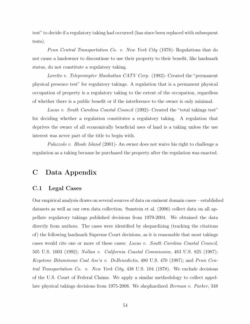
test” to decide if a regulatory taking had occurred (has since been replaced with subsequent

tests).

Penn Central Transportation Co. v. New York City (1978)- Regulations that do

not cause a landowner to discontinue to use their property to their benefit, like landmark

status, do not constitute a regulatory taking.

Loretto v. Teleprompter Manhattan CATV Corp. (1982)- Created the “permanent

physical presence test” for regulatory takings. A regulation that is a permanent physical

occupation of property is a regulatory taking to the extent of the occupation, regardless

of whether there is a public benefit or if the interference to the owner is only minimal.

Lucas v. South Carolina Coastal Council (1992)- Created the “total takings test”

for deciding whether a regulation constitutes a regulatory taking. A regulation that

deprives the owner of all economically beneficial uses of land is a taking unless the use

interest was never part of the title to begin with.

Palazzolo v. Rhode Island (2001)- An owner does not waive his right to challenge a

regulation as a taking because he purchased the property after the regulation was enacted.

C Data Appendix

C.1 Legal Cases

Our empirical analysis draws on several sources of data on eminent domain cases—established

datasets as well as our own data collection. Sunstein et al. (2006) collect data on all ap-

pellate regulatory takings published decisions from 1979-2004. We obtained the data

directly from authors. The cases were identified by shepardizing (tracking the citations

of) the following landmark Supreme Court decisions, as it is reasonable that most takings

cases would cite one or more of these cases: Lucas v. South Carolina Coastal Council,

505 U.S. 1003 (1992); Nollan v. California Coastal Commission, 483 U.S. 825 (1987);

Keystone Bituminous Coal Ass’n v. DeBenedictis, 480 U.S. 470 (1987); and Penn Cen-

tral Transportation Co. v. New York City, 438 U.S. 104 (1978). We exclude decisions

of the U.S. Court of Federal Claims. We apply a similar methodology to collect appel-

late physical takings decisions from 1975-2008. We shephardized Berman v. Parker, 348

54

U.S. 26 (1954); Hawaii Housing Authority v. Midkiff, 467 U.S. 229 (1984); Loretto v.

Teleprompter Manhattan CATV Corp., 458 U.S. 419 (1982); Kelo v. City of New London,

545 U.S. 469 (2005); Yee v. City of Escondido, 503 U.S. 519 (1992). Our physical takings

data collection actually goes back to the 1950s, but our outcomes dataset begins in 1975.

This extension does allow us to estimate models with more distributed lags without loss

of observations.

Following Sunstein et al. (2006) , we code a vote as pro-plaintiff if the judge voted

to grant the party alleging a violation of the Takings Clause any relief. The sample

includes only cases that had substantive decisions about takings, rather than cases that

were decided only on procedural grounds. Figure 2 plots the quantity of eminent domain

cases that were decided pro-plaintiff or pro-defendant (i.e. government) during this time

period. Table 1 indicates that on average there are 0.71 regulatory takings panels per

circuit-year for a total of 220 cases and 0.33 physical takings panels per circuit-year for

a total of 134 cases. A sizeable portion of circuit-years, 54%, had no regulatory takings

panel; 74% of circuit-years had no physical takings panel. Three-quarters of the regulatory

takings decisions and two-thirds of the physical takings decisions are pro-government.

In addition to appellate takings cases, our third and fourth datasets comprise all

district court cases involving regulatory and physical takings .On Westlaw, we shepardize

the same Supreme Court cases that we used to construct the appellate databases. This

resulted in 498 regulatory takings cases from 1979-2004 and 635 physical takings cases

from 1975-2008.

C.2 Judicial Biographies

We collect information on judge characteristics from several sources. We begin with

the Appeals Court Attribute Data compiled by Zuk, Barrow, and Gryski.61 These data

cover nearly all judges appointed to federal appeals courts and federal district courts

from 1789 to 2000 and provide partial information through 2004. The dataset includes

information on vital statistics, geographic history, education, occupational history and

governmental positions, military service, religion, race, gender, political affiliations, and

other variables. For appellate judges with missing information, we first filled in their61http://www.cas.sc.edu/poli/juri/attributes.html

55

entries with data from the Auburn District Court database, provided that the judge had

occupied a district court seat prior to 2000. But because these data do not cover many

George W. Bush appointees, we used the Federal Judicial Center website62 for information

on a judge’s birth, geographic origin, gender, education, occupational history and political

appointments. We obtained religion data on Reagan- and post-Reagan judicial appointees

from Goldman and from Sisk63 and searched transcripts of Congressional confirmation

hearings and other official or news publications on Lexis to fill in the rest of the missing

religion variables. We coded the judges whose religions remained missing or unknown as

having no publicly known religious affiliation. The average circuit-year has 17.81 judges

available for assignment to panels. Appellate-level judges typically sit on three-judge

appellate panels, though some judges in the appellate-level pool come from district courts

or specialized courts. We drop these outside judges from our probability calculations, as

they are rare. In expectation, there are 0.06 black judges per seat (or 0.18 black judges

on a 3-judge panel), 0.06 minority Democratic appointees per seat, and 0.07 prior U.S.

Attorney Republican appointees per seat (Table 1). We calculate the expectations based

on the frequency the typical senior judge sits on cases and weigh senior judges accordingly.

C.3 Property Prices Data

Our main outcome variables are property values (house price indices) at the zip code

level from the Fiserv Case-Shiller Weiss data, which cover the entire United States. We

use these data to construct a panel of about 40,000 zip codes followed quarterly from

1975 to 2008. The Fiserv Case-Shiller Weiss indices are based on repeat sales data on

single-family homes. In geographic areas that do not have a valid Case-Shiller price index,

Fiserv splices in the corresponding Federal Housing Finance Agency (FHFA) index. The

FHFA series is a quarterly, weighted, repeat-sales single family house price index based on

repeat mortgage transactions handled by Fannie Mae or Freddie Mac. Because the Fiserv

index requires a significant number of transactions in an area, the zip code-specific price

indices are concentrated in metropolitan areas. Where zip code-specific price indices are62http://www.fjc.gov/history/home.nsf.63Raw data from Goldman (1997) were obtained directly from the author. Sisk’s data are available at

http://courseweb.stthomas.edu/gcsisk/religion.study.data/cover.htm

56

unavailable, we substitute with the price index for the next geographic level, e.g., county,

then division, CBSA, or state. In robustness checks, we weigh the zip codes using zip

code specific population estimates calculated for 2005 from the U.S. Census; the Census

data documentation is located at: http://www.census.gov/prod/cen2000/doc/sf1.pdf. In

unreported results, we also conduct analyses separately for metropolitan areas only, as

well as restrict analyses to only those zip codes with zip-code specific price indices and

find our main results to be robust, suggesting that our results are primarily driven by

metropolitan-level price outcomes.

C.4 Other Outcomes Data

We use the March Current Population Survey (CPS) for housing outcomes, such as

whether an individual owns or rents, whether an individual lives in public housing, and

whether an individual lives below the poverty line. We use the Merged Outgoing Rota-

tion Groups (MORG) CPS for employment outcomes, such as weekly earnings, amount

of time worked, and employment status. The CPS provides point-in-time measures of the

individual-level variables, including age, sex, race, marital status, educational attainment,

and the geographic location of the individual, which lets us match the state of residence

to the circuit having legal jurisdiction. We restrict our sample to individuals between the

ages of 18 and 65 and weight our analysis with March CPS person weights for individual

housing outcomes and MORG earnings weights for employment outcomes. Data on gross

domestic product (GDP) by state were obtained from the Bureau of Economic Analysis;

estimates are aggregated across all industries by year.64

D Randomization

Our empirical strategy involves using the number of black judges assigned to regulatory

takings cases to approximate a true experiment. This requires that appellate judges

be randomly assigned to takings appeals. While random assignment is the standard

procedure according to court administrators, some scholars argue that certain circuits

have not always followed this (Hall (2010)). For our identification, at the circuit-year64http://www.bea.gov/regional/gsp/default.cfm#download.

57

level, the number of black judges per seat needs to be as good as randomly assigned,

conditional on having an appeal.

We check the randomization assumption in two ways. First, in previous work, we

surveyed courts of appeals and evaluated the courts’ measures to ensure that the assign-

ment of judges to panels is random (Chen and Sethi (2011)). As a second randomization

check, we examine whether the sequence of actual numbers of black judges per seat is like

a random process. These checks are important because the decision to publish an opinion

may introduce non-randomness.65 For example, the decision not to publish may be a

compromise among judges who disagree about the correct outcome (Law (2005), Wald

(1999)). If black judges publish and non-black judges choose not to publish regulatory

takings decisions, then a correlation may arise between the egregiousness of the eminent

domain case and the judicial panel composition. This correlation could reintroduce possi-

ble endogeneity between social trends related to the egregiousness of eminent domain cases

and the panel composition of published cases. Thus, examining whether characteristics

of the case determined by lower courts are unrelated to the composition of the appellate

panel helps assess this concern. Moreover, if panel composition significantly affects the

decision to publish, panel composition of published cases would be serially correlated.

Figure 3 suggests visually that panel composition is not serially correlated. For-

mally, the general approach to assessing randomness is analogous to a Fisher exact test,

except that we use simulations. The methodology we follow is:

1. Propose a statistic that can be computed from the sequence of numbers of black

judges per seat within a circuit.

2. Compute the statistic for the actual sequence, s⇤.

3. Compute the statistic for each of 1,000 bootstrap samples from the actual sequence,

i.e., s1, s2, s3 . . . sn. Since there were changes in the expected number of black

judges per seat over time, we treat our bootstrap samples as a vector of realized65More specifically, the editorial decision to be included in Westlaw or Lexis is left to the discretion

of the individual companies for unpublished cases. Many “unpublished” cases are actually published.Even if editors desire to be as inclusive as possible, some decisions may go truly undetected. If judgesgrant motions for summary judgment, the opinion would not cite the SCOTUS case. Therefore, it isimportant to check for randomization.

58

random variables, with the probability based on the expectation during the circuit-

year.

4. Compute the empirical p-value, pi by determining where s⇤ fits into s1, s2, s3 . . .

sn.

5. Repeat steps 1-4 and calculate pi for each unit.

We use the following statistics:

Autocorrelation: We see if the value in the jth case depends on the outcome

in the j-1thcase. This statistic can detect whether judicial assignments are “clustered,”

meaning a higher than expected number of back-to-back high number of seat assignments

to a black judge. This test tells us whether certain judges sought out eminent domain

cases, perhaps in sequence.

Mean-Reversion: We test whether there is any form of mean reversion in the

sequence, meaning that the assignment in the nth case is correlated with the assignment in

previous n� 1 cases. This test tells us whether judges or their assignors were attempting

to equilibrate their presence, considering whether a judge was “due” for a eminent domain

case.

Longest-Run: We test whether there are abnormally long “runs” of number of

black judges per seat. This test tells us whether certain circuits may have assigned certain

judges with eminent domain cases during certain time periods, for example, to achieve

specialization.66

While this process generates a collection of p-values, it is not intuitively obvious

what the rejection criteria should be. Since p-values from a truly random process with

a sufficient number of possible states is uniformly distributed, even with just 10 units

and 3 statistics, the probability of not having even one p-value less than .025 or greater

than .975 is only about 21%. With a truly random process, collection of all unit p-values

should be uniformly distributed. (Imagine that you generate summary statistics for 1000

random strings. The 1001th random string should have a summary statistic that is equally

likely to be anywhere from 1 to 1000.) Of course, since there are only 12 units, we would66Some sources suggest that courts do batch cases dealing with similar issues to one panel in order to

dispose of cases more quickly and without duplication of effort (Wallace (2005)).

59

not expect a kernel density estimate to “look” uniform. We use Kolmogorov-Smirnov Test

to test whether the empirical distribution of p-values approaches the CDF of a uniform

distribution using the one-sided critical value with n = 12.67 The intuition is to simply

add up the space between the 45-degree line representing a uniform distribution and the p

values displayed in Appendx Figure A2. We plot the empirical distribution for our 3 test

statistics and one set of instruments each for regulatory takings and physical takings in

Appendix Figure A2. Appendix Table A1 confirms the visual intuition that our p-values

are uniformly distributed for all 6 tests.

67http://www.ciphersbyritter.com/JAVASCRP/NORMCHIK.HTM#KolSmir.

60

Circuit-Year Level

Mean [Standard Deviation]

Regulatory Takings Cases (1979-2004)Number of Judges 17.813

[7.457]

Number of Regulatory Takings Panels 0.71[0.988]

Proportion of Circuit-Years with No Regulatory Takings Panels 54%

Proportion of Pro-Government Regulatory Takings Decisions when Circuit-Year has Panels 78%

Expected # of Black Judges per Seat 0.06[0.056]

N (circuit-years) 310Physical Takings Cases (1975-2008)

Number of Judges 17.662[7.719]

Number of Physical Takings Panels 0.333[0.630]

Proportion of Circuit-Years with No Physical Takings Panels 73%

Proportion of Pro-Government Physical Takings Decisions when Circuit-Year has Panels 66%

Expected # of Minority Judges per Seat 0.086[0.066]

Expected # of Democratic Appointees per Seat 0.418[0.129]

Expected # of Prior US Attorneys per Seat 0.071[0.081]

Expected # of Democratic Minority Appointees per Seat 0.064[0.059]

Expected # Republican Prior US Attorneys per Seat 0.038[0.062]

N (circuit-years) 402

Table 1 - Summary Statistics

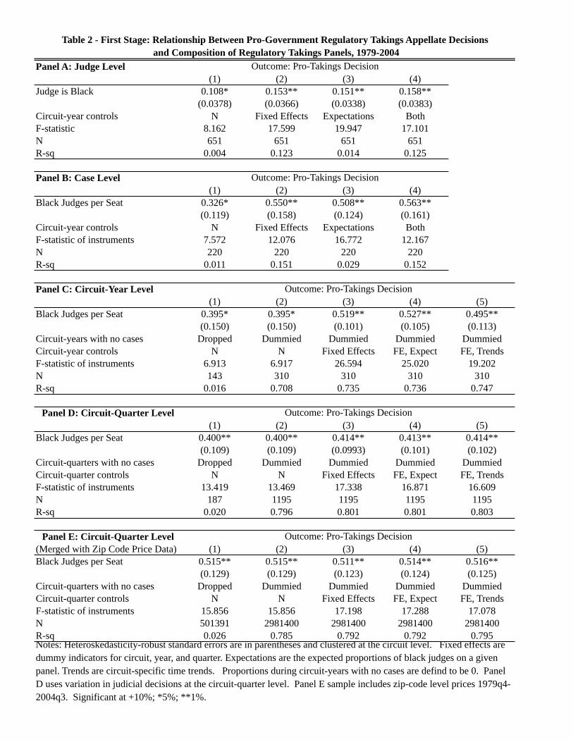
Panel A: Judge Level(1) (2) (3) (4)

Judge is Black 0.108* 0.153** 0.151** 0.158**(0.0378) (0.0366) (0.0338) (0.0383)

Circuit-year controls N Fixed Effects Expectations BothF-statistic 8.162 17.599 19.947 17.101N 651 651 651 651R-sq 0.004 0.123 0.014 0.125

Panel B: Case Level(1) (2) (3) (4)

Black Judges per Seat 0.326* 0.550** 0.508** 0.563**(0.119) (0.158) (0.124) (0.161)

Circuit-year controls N Fixed Effects Expectations BothF-statistic of instruments 7.572 12.076 16.772 12.167N 220 220 220 220R-sq 0.011 0.151 0.029 0.152

Panel C: Circuit-Year Level(1) (2) (3) (4) (5)

Black Judges per Seat 0.395* 0.395* 0.519** 0.527** 0.495**(0.150) (0.150) (0.101) (0.105) (0.113)

Circuit-years with no cases Dropped Dummied Dummied Dummied DummiedCircuit-year controls N N Fixed Effects FE, Expect FE, TrendsF-statistic of instruments 6.913 6.917 26.594 25.020 19.202N 143 310 310 310 310R-sq 0.016 0.708 0.735 0.736 0.747

Panel D: Circuit-Quarter Level(1) (2) (3) (4) (5)

Black Judges per Seat 0.400** 0.400** 0.414** 0.413** 0.414**(0.109) (0.109) (0.0993) (0.101) (0.102)

Circuit-quarters with no cases Dropped Dummied Dummied Dummied DummiedCircuit-quarter controls N N Fixed Effects FE, Expect FE, TrendsF-statistic of instruments 13.419 13.469 17.338 16.871 16.609N 187 1195 1195 1195 1195R-sq 0.020 0.796 0.801 0.801 0.803

Panel E: Circuit-Quarter Level(Merged with Zip Code Price Data) (1) (2) (3) (4) (5)Black Judges per Seat 0.515** 0.515** 0.511** 0.514** 0.516**

(0.129) (0.129) (0.123) (0.124) (0.125)Circuit-quarters with no cases Dropped Dummied Dummied Dummied DummiedCircuit-quarter controls N N Fixed Effects FE, Expect FE, TrendsF-statistic of instruments 15.856 15.856 17.198 17.288 17.078N 501391 2981400 2981400 2981400 2981400R-sq 0.026 0.785 0.792 0.792 0.795

Outcome: Pro-Takings Decision

and Composition of Regulatory Takings Panels, 1979-2004Table 2 - First Stage: Relationship Between Pro-Government Regulatory Takings Appellate Decisions

Outcome: Pro-Takings Decision

Outcome: Pro-Takings Decision

Notes: Heteroskedasticity-robust standard errors are in parentheses and clustered at the circuit level. Fixed effects are dummy indicators for circuit, year, and quarter. Expectations are the expected proportions of black judges on a given panel. Trends are circuit-specific time trends. Proportions during circuit-years with no cases are defind to be 0. Panel D uses variation in judicial decisions at the circuit-quarter level. Panel E sample includes zip-code level prices 1979q4-2004q3. Significant at +10%; *5%; **1%.

Outcome: Pro-Takings Decision

Outcome: Pro-Takings Decision

Panel A: Judge Level(1) (2) (3) (4) (5) (6)

Democratic, Minority -0.203* -0.258* -0.154+ -0.198 -0.112+(0.0686) (0.113) (0.0755) (0.125) (0.0552)

Republican, Prior US Attorney 0.176* 0.153+ 0.0859 0.134+ 0.0647(0.0741) (0.0748) (0.0827) (0.0654) (0.0902)

Circuit-year controls N N N Fixed Effects Expectations BothF-statistic 8.800 5.638 4.367 5.010 4.092 4.260N 394 307 307 307 307 307R-sq 0.017 0.008 0.031 0.359 0.054 0.398

Panel B: Case Level(1) (2) (3) (4)

Democratic, Minority Appointees -0.570* -0.573** -0.551* -0.426* per Seat (0.186) (0.182) (0.249) (0.188)Republican, Prior US Attorneys 0.677* 0.610 0.598+ 0.502 per Seat (0.235) (0.515) (0.272) (0.545)Circuit-year controls N Fixed Effects Expectations BothF-statistic of instruments 12.540 14.429 9.978 4.239N 134 134 134 134R-sq 0.076 0.388 0.079 0.410

Panel C: Circuit-Year Level(1) (2) (3) (4) (5)

Democratic, Minority Appointees -0.615** -0.615** -0.655** -0.666** -0.651** per Seat (0.193) (0.191) (0.172) (0.177) (0.160)Republican, Prior US Attorneys 0.929** 0.929** 0.969** 0.963** 1.032** per Seat (0.272) (0.270) (0.233) (0.231) (0.212)Circuit-years with no cases Dropped Dummied Dummied Dummied DummiedCircuit-year controls N N Fixed Effects FE, Expect FE, TrendsF-statistic of instruments 9.010 9.114 15.178 15.220 19.239N 107 402 402 402 402R-sq 0.108 0.651 0.692 0.693 0.705

Panel D: Circuit-Quarter Level(1) (2) (3) (4) (5)

Democratic, Minority Appointees -0.547* -0.547* -0.561** -0.563** -0.561** per Seat (0.184) (0.182) (0.175) (0.176) (0.171)Republican, Prior US Attorneys 0.707* 0.707* 0.703* 0.702* 0.717** per Seat (0.232) (0.230) (0.232) (0.232) (0.229)Circuit-quarters with no cases Dropped Dummied Dummied Dummied DummiedCircuit-quarter controls N N Fixed Effects FE, Expect FE, TrendsF-statistic of instruments 12.357 12.530 12.991 13.039 13.349N 129 1608 1608 1608 1608R-sq 0.075 0.680 0.690 0.690 0.693

Panel E: Circuit-Quarter Level(Merged with Zip Code Price Data) (8) (9) (10) (11) (12)Democratic, Minority Appointees -0.518* -0.518* -0.534* -0.534* -0.533** per Seat (0.184) (0.184) (0.175) (0.174) (0.168)Republican, Prior US Attorneys 0.553* 0.553* 0.542* 0.540* 0.555* per Seat (0.215) (0.215) (0.215) (0.216) (0.211)Circuit-quarters with no cases Dropped Dummied Dummied Dummied DummiedCircuit-quarter controls N N Fixed Effects FE, Expect FE, TrendsF-statistic of instruments 34.975 34.976 40.946 42.747 41.925N 357691 4054704 4054704 4054704 4054704R-sq 0.062 0.676 0.686 0.686 0.689Notes: Heteroskedasticity-robust standard errors are in parentheses and clustered at the circuit level. Fixed effects are dummy indicators for circuit, year, and quarter. Expectations are the expected proportions that are minority Democratic appointees or prior US attorney Republican appointees on a given panel. Trends are circuit-specific time trends. Proportions during circuit-years with no cases are defind to be 0. Panel D uses variation in judicial decisions at the circuit-quarter level. Panel E sample includes zip-code level prices 1975q1-2008q4. Significant at +10%; *5%; **1%.

Outcome: Pro-Takings Decision

Table 3 - First Stage: Relationship Between Pro-Government Physical Takings Appellate Decisions and Composition of Physical Takings Panels, 1975-2008

Outcome: Pro-Takings Decision

Outcome: Pro-Takings Decision

Outcome: Pro-Takings Decision

Outcome: Pro-Takings Decision

Dependent Variable(1) (2) (3) (4) (5) (6) (7) (8) (9)

Proportion Pro-Taking -0.00349** -0.00192 -0.00951+ 0.00429 0.00203 0.0102 0.00679 0.0206 0.0106 Appellate Decisionst+1 (0.000985) (0.00932) (0.00517) (0.00500) (0.00210) (0.0139) (0.0215) (0.0227) (0.0204)Proportion Pro-Taking 0.00156 -0.0108 -0.00615 0.0119* 0.00652 0.0155 0.00503 0.0153+ -0.00131 Appellate Decisionst (0.00232) (0.0116) (0.00591) (0.00593) (0.00687) (0.0283) (0.0150) (0.00914) (0.00822)Proportion Pro-Taking 0.00201 0.00419 0.00500 0.00152 0.00132 0.00120 0.00368 0.0132 0.0114+ Appellate Decisionst-1 (0.00135) (0.0133) (0.00715) (0.00794) (0.00623) (0.0166) (0.0156) (0.0127) (0.00665)Proportion Pro-Taking 0.000963 0.0111 0.00676 -0.00281 -0.00330 0.0109 -0.0112 0.00299 0.00419 Appellate Decisionst-2 (0.00102) (0.00966) (0.00987) (0.00680) (0.00496) (0.0154) (0.0156) (0.0178) (0.0159)Proportion Pro-Taking 0.00273 0.0166 0.00887 0.00680 -0.000192 -0.00738 -0.000768 0.000989 -0.00523 Appellate Decisionst-3 (0.00158) (0.0159) (0.00564) (0.00783) (0.00456) (0.0206) (0.0153) (0.0108) (0.0110)Proportion Pro-Taking 0.00257+ 0.00474 0.00524+ 0.00874* 0.00934 0.00525 -0.00528 0.0149 0.00887 Appellate Decisionst-4 (0.00121) (0.00867) (0.00292) (0.00361) (0.00599) (0.0150) (0.0178) (0.0276) (0.0188)Appellate IV N Y Y Lasso IV Lasso IV Y Y Lasso IV Lasso IVDistrict IV N N Lasso IV N Lasso IV N Lasso IV N Lasso IVAggregation Level Zip-Year Zip-Year Zip-Year Zip-Year Zip-Year Circuit-Year Circuit-Year Circuit-Year Circuit-YearN 2486744 2486744 2486744 2486744 2486744 250 250 250 250R-sq 0.082 . 0.024 0.042 0.044 0.197 0.111 0.048 0.087Mean dependent variable 0.011 0.011 0.011 0.011 0.011 0.013 0.013 0.013 0.013Average lag effect 0.002 0.005 0.004 0.005 0.003 0.005 -0.002 0.009 0.004 P-value of lags 0.086 0.001 0.208 0.000 0.000 0.963 0.958 0.000 0.050 P-value of leads 0.005 0.837 0.066 0.390 0.333 0.464 0.752 0.363 0.606Average lag of no appeal 0.003 0.005 0.002 0.005 0.002 0.005 -0.005 0.008 -0.002 P-value of no appeal lags 0.208 0.029 0.373 0.000 0.101 0.965 0.479 0.003 0.093 P-value of unconditional (Lawct + 1[Mct > 0]) lags 0.532 0.000 0.095 0.164 0.000 0.965 0.118 0.447 0.025Typical Conditional effect 0.0008 0.0021 0.0017 0.0021 0.0013 0.0021 -0.0008 0.0038 0.0017 Unconditional effect - pro -0.0003 0.0002 0.0009 0.0002 0.0005 0.0002 0.0011 0.0007 0.0025 Unconditional effect - anti -0.0004 -0.0007 -0.0003 -0.0007 -0.0003 -0.0007 0.0007 -0.0011 0.0003 Unconditional effect - all -0.0008 -0.0006 0.0006 -0.0006 0.0002 -0.0006 0.0019 -0.0005 0.0028

Dependent Variable(1) (2) (3) (4) (5) (6) (7) (8) (9)

Proportion Pro-Taking 0.00402 0.00285 0.00166 -0.00212 -0.00258 0.00647 0.000831 0.00616 0.00379 Appellate Decisionst+1 (0.00230) (0.00428) (0.00408) (0.00703) (0.0100) (0.00492) (0.00437) (0.00387) (0.00482)Proportion Pro-Taking 0.00499* 0.00955+ 0.0121** 0.0139* -0.00000577 0.00860 0.0106+ 0.0140** 0.0100* Appellate Decisionst (0.00193) (0.00557) (0.00445) (0.00647) (0.00552) (0.00583) (0.00549) (0.00447) (0.00436)Proportion Pro-Taking 0.00296* 0.0136** 0.0112** 0.00147 0.00353 0.0124* 0.0118** 0.0141** 0.00869* Appellate Decisionst-1 (0.00133) (0.00396) (0.00364) (0.00679) (0.00490) (0.00506) (0.00399) (0.00513) (0.00428)Proportion Pro-Taking 0.00330* 0.0190** 0.00872 0.00478 0.00507 0.0211** 0.0105 0.00985** 0.00567 Appellate Decisionst-2 (0.00133) (0.00326) (0.00566) (0.00390) (0.00804) (0.00427) (0.00681) (0.00363) (0.00539)Proportion Pro-Taking 0.00159 0.0124** 0.00652 -0.00393 -0.000501 0.0196** 0.00906 0.00367 0.00256 Appellate Decisionst-3 (0.00166) (0.00410) (0.00547) (0.00749) (0.00401) (0.00617) (0.00719) (0.00444) (0.00594)Proportion Pro-Taking -0.000393 0.00552** -0.00342 0.00573 0.00291 0.00478 -0.00633 -0.001000 -0.00302 Appellate Decisionst-4 (0.00129) (0.00165) (0.00443) (0.0107) (0.00903) (0.00420) (0.00596) (0.00280) (0.00431)Appellate IV N Y Y Lasso IV Lasso IV Y Y Lasso IV Lasso IVDistrict IV N N Lasso IV N Lasso IV N Lasso IV N Lasso IVAggregation Level Zip-Year Zip-Year Zip-Year Zip-Year Zip-Year Circuit-Year Circuit-Year Circuit-Year Circuit-YearN 3989626 3989626 3989626 3989626 3989626 398 398 398 398R-sq 0.112 0.080 0.099 0.103 0.087 0.429 0.525 0.538 0.566Mean dependent variable 0.012 0.012 0.012 0.012 0.012 0.013 0.013 0.013 0.013Average lag effect 0.002 0.012 0.007 0.004 0.002 0.013 0.007 0.008 0.005 P-value of lags 0.032 0.000 0.001 0.101 0.883 0.000 0.000 0.002 0.000 P-value of leads 0.108 0.505 0.684 0.763 0.797 0.189 0.849 0.112 0.432Average lag of no appeal 0.003 0.010 0.006 0.004 0.003 0.010 0.005 0.006 0.003 P-value of no appeal lags 0.094 0.000 0.153 0.286 0.002 0.000 0.000 0.208 0.532 P-value of unconditional (Lawct + 1[Mct > 0]) lags 0.000 0.000 0.000 0.015 0.060 0.000 0.000 0.000 0.029Typical Conditional effect 0.0004 0.0021 0.0012 0.0007 0.0004 0.0023 0.0012 0.0014 0.0009 Unconditional effect - pro -0.0001 0.0005 0.0003 0.0001 -0.0001 0.0007 0.0004 0.0005 0.0004 Unconditional effect - anti -0.0002 -0.0008 -0.0005 -0.0003 -0.0002 -0.0008 -0.0004 -0.0005 -0.0002 Unconditional effect - all -0.0005 -0.0006 -0.0004 -0.0004 -0.0005 -0.0004 -0.0001 -0.0002 0.0001

Table 4 - The Effect of Takings Precedents on House PricesPanel A. Regulatory Takings

Notes: Significant at +10%, *5%, **1%. Notes: Data consist of Fiserv Case-Shiller/FHFA zip-code level price indices. Heteroskedasticity-robust standard errors are in parentheses and clustered by circuit. Regressions include circuit fixed effects, year and quarter fixed effects, a dummy for whether there were no cases in that circuit-year. Instruments for appellate regulatory takings are Black judges per seat assigned to regulatory takings cases in a circuit-year. Instruments for appellate physical takings are Democratic Non-White Appointees per seat and Republican Prior US Attorneys per seat assigned to physical takings cases in a circuit-year. LASSO instruments are displayed in Appendix Table A3.

ΔLog Price Index

Panel B. Physical TakingsΔLog Price Index

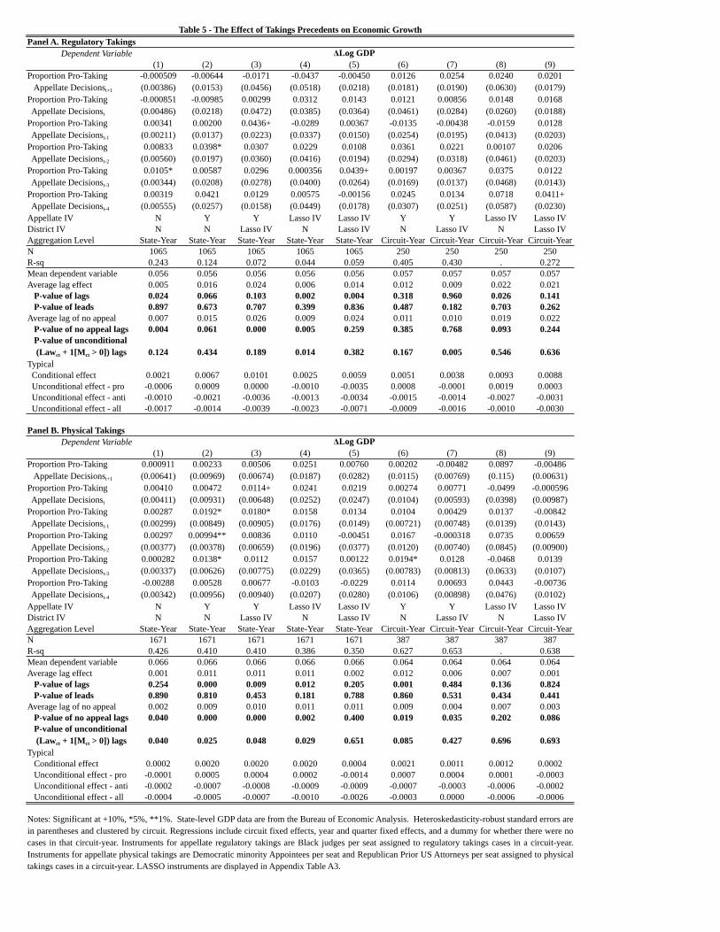
Dependent Variable(1) (2) (3) (4) (5) (6) (7) (8) (9)

Proportion Pro-Taking -0.000509 -0.00644 -0.0171 -0.0437 -0.00450 0.0126 0.0254 0.0240 0.0201 Appellate Decisionst+1 (0.00386) (0.0153) (0.0456) (0.0518) (0.0218) (0.0181) (0.0190) (0.0630) (0.0179)Proportion Pro-Taking -0.000851 -0.00985 0.00299 0.0312 0.0143 0.0121 0.00856 0.0148 0.0168 Appellate Decisionst (0.00486) (0.0218) (0.0472) (0.0385) (0.0364) (0.0461) (0.0284) (0.0260) (0.0188)Proportion Pro-Taking 0.00341 0.00200 0.0436+ -0.0289 0.00367 -0.0135 -0.00438 -0.0159 0.0128 Appellate Decisionst-1 (0.00211) (0.0137) (0.0223) (0.0337) (0.0150) (0.0254) (0.0195) (0.0413) (0.0203)Proportion Pro-Taking 0.00833 0.0398* 0.0307 0.0229 0.0108 0.0361 0.0221 0.00107 0.0206 Appellate Decisionst-2 (0.00560) (0.0197) (0.0360) (0.0416) (0.0194) (0.0294) (0.0318) (0.0461) (0.0203)Proportion Pro-Taking 0.0105* 0.00587 0.0296 0.000356 0.0439+ 0.00197 0.00367 0.0375 0.0122 Appellate Decisionst-3 (0.00344) (0.0208) (0.0278) (0.0400) (0.0264) (0.0169) (0.0137) (0.0468) (0.0143)Proportion Pro-Taking 0.00319 0.0421 0.0129 0.00575 -0.00156 0.0245 0.0134 0.0718 0.0411+ Appellate Decisionst-4 (0.00555) (0.0257) (0.0158) (0.0449) (0.0178) (0.0307) (0.0251) (0.0587) (0.0230)Appellate IV N Y Y Lasso IV Lasso IV Y Y Lasso IV Lasso IVDistrict IV N N Lasso IV N Lasso IV N Lasso IV N Lasso IVAggregation Level State-Year State-Year State-Year State-Year State-Year Circuit-Year Circuit-Year Circuit-Year Circuit-YearN 1065 1065 1065 1065 1065 250 250 250 250R-sq 0.243 0.124 0.072 0.044 0.059 0.405 0.430 . 0.272Mean dependent variable 0.056 0.056 0.056 0.056 0.056 0.057 0.057 0.057 0.057Average lag effect 0.005 0.016 0.024 0.006 0.014 0.012 0.009 0.022 0.021 P-value of lags 0.024 0.066 0.103 0.002 0.004 0.318 0.960 0.026 0.141 P-value of leads 0.897 0.673 0.707 0.399 0.836 0.487 0.182 0.703 0.262Average lag of no appeal 0.007 0.015 0.026 0.009 0.024 0.011 0.010 0.019 0.022 P-value of no appeal lags 0.004 0.061 0.000 0.005 0.259 0.385 0.768 0.093 0.244 P-value of unconditional (Lawct + 1[Mct > 0]) lags 0.124 0.434 0.189 0.014 0.382 0.167 0.005 0.546 0.636Typical Conditional effect 0.0021 0.0067 0.0101 0.0025 0.0059 0.0051 0.0038 0.0093 0.0088 Unconditional effect - pro -0.0006 0.0009 0.0000 -0.0010 -0.0035 0.0008 -0.0001 0.0019 0.0003 Unconditional effect - anti -0.0010 -0.0021 -0.0036 -0.0013 -0.0034 -0.0015 -0.0014 -0.0027 -0.0031 Unconditional effect - all -0.0017 -0.0014 -0.0039 -0.0023 -0.0071 -0.0009 -0.0016 -0.0010 -0.0030

Dependent Variable(1) (2) (3) (4) (5) (6) (7) (8) (9)

Proportion Pro-Taking 0.000911 0.00233 0.00506 0.0251 0.00760 0.00202 -0.00482 0.0897 -0.00486 Appellate Decisionst+1 (0.00641) (0.00969) (0.00674) (0.0187) (0.0282) (0.0115) (0.00769) (0.115) (0.00631)Proportion Pro-Taking 0.00410 0.00472 0.0114+ 0.0241 0.0219 0.00274 0.00771 -0.0499 -0.000596 Appellate Decisionst (0.00411) (0.00931) (0.00648) (0.0252) (0.0247) (0.0104) (0.00593) (0.0398) (0.00987)Proportion Pro-Taking 0.00287 0.0192* 0.0180* 0.0158 0.0134 0.0104 0.00429 0.0137 -0.00842 Appellate Decisionst-1 (0.00299) (0.00849) (0.00905) (0.0176) (0.0149) (0.00721) (0.00748) (0.0139) (0.0143)Proportion Pro-Taking 0.00297 0.00994** 0.00836 0.0110 -0.00451 0.0167 -0.000318 0.0735 0.00659 Appellate Decisionst-2 (0.00377) (0.00378) (0.00659) (0.0196) (0.0377) (0.0120) (0.00740) (0.0845) (0.00900)Proportion Pro-Taking 0.000282 0.0138* 0.0112 0.0157 0.00122 0.0194* 0.0128 -0.0468 0.0139 Appellate Decisionst-3 (0.00337) (0.00626) (0.00775) (0.0229) (0.0365) (0.00783) (0.00813) (0.0633) (0.0107)Proportion Pro-Taking -0.00288 0.00528 0.00677 -0.0103 -0.0229 0.0114 0.00693 0.0443 -0.00736 Appellate Decisionst-4 (0.00342) (0.00956) (0.00940) (0.0207) (0.0280) (0.0106) (0.00898) (0.0476) (0.0102)Appellate IV N Y Y Lasso IV Lasso IV Y Y Lasso IV Lasso IVDistrict IV N N Lasso IV N Lasso IV N Lasso IV N Lasso IVAggregation Level State-Year State-Year State-Year State-Year State-Year Circuit-Year Circuit-Year Circuit-Year Circuit-YearN 1671 1671 1671 1671 1671 387 387 387 387R-sq 0.426 0.410 0.410 0.386 0.350 0.627 0.653 . 0.638Mean dependent variable 0.066 0.066 0.066 0.066 0.066 0.064 0.064 0.064 0.064Average lag effect 0.001 0.011 0.011 0.011 0.002 0.012 0.006 0.007 0.001 P-value of lags 0.254 0.000 0.009 0.012 0.205 0.001 0.484 0.136 0.824 P-value of leads 0.890 0.810 0.453 0.181 0.788 0.860 0.531 0.434 0.441Average lag of no appeal 0.002 0.009 0.010 0.011 0.011 0.009 0.004 0.007 0.003 P-value of no appeal lags 0.040 0.000 0.000 0.002 0.400 0.019 0.035 0.202 0.086 P-value of unconditional (Lawct + 1[Mct > 0]) lags 0.040 0.025 0.048 0.029 0.651 0.085 0.427 0.696 0.693Typical Conditional effect 0.0002 0.0020 0.0020 0.0020 0.0004 0.0021 0.0011 0.0012 0.0002 Unconditional effect - pro -0.0001 0.0005 0.0004 0.0002 -0.0014 0.0007 0.0004 0.0001 -0.0003 Unconditional effect - anti -0.0002 -0.0007 -0.0008 -0.0009 -0.0009 -0.0007 -0.0003 -0.0006 -0.0002 Unconditional effect - all -0.0004 -0.0005 -0.0007 -0.0010 -0.0026 -0.0003 0.0000 -0.0006 -0.0006

Panel B. Physical Takings

Panel A. Regulatory TakingsTable 5 - The Effect of Takings Precedents on Economic Growth

ΔLog GDP

ΔLog GDP

Notes: Significant at +10%, *5%, **1%. State-level GDP data are from the Bureau of Economic Analysis. Heteroskedasticity-robust standard errors arein parentheses and clustered by circuit. Regressions include circuit fixed effects, year and quarter fixed effects, and a dummy for whether there were nocases in that circuit-year. Instruments for appellate regulatory takings are Black judges per seat assigned to regulatory takings cases in a circuit-year.Instruments for appellate physical takings are Democratic minority Appointees per seat and Republican Prior US Attorneys per seat assigned to physicaltakings cases in a circuit-year. LASSO instruments are displayed in Appendix Table A3.

Dependent Variable(1) (2) (3) (4) (5) (6) (7) (8)

Proportion Pro-Taking 0.00131 -0.00879* -0.00915 0.00355 0.00438 0.00538 0.00236 -0.0148 Appellate Decisionst+1 (0.00338) (0.00377) (0.0137) (0.0150) (0.00268) (0.00583) (0.00479) (0.0112)Proportion Pro-Taking 0.0106** 0.0128+ 0.0204* 0.0257 0.00476* 0.0111+ 0.0128** -0.00533 Appellate Decisionst (0.00310) (0.00773) (0.00980) (0.0157) (0.00165) (0.00652) (0.00386) (0.0203)Proportion Pro-Taking 0.0131** 0.0121 0.0103* 0.00621 0.00433* 0.00369 0.00643 -0.00380 Appellate Decisionst-1 (0.00350) (0.00957) (0.00485) (0.0252) (0.00180) (0.00434) (0.00486) (0.0167)Proportion Pro-Taking 0.00435 -0.00353 -0.00395 0.0211 0.00577* 0.00872* 0.00802 0.0187 Appellate Decisionst-2 (0.00400) (0.0101) (0.00984) (0.0293) (0.00202) (0.00395) (0.00555) (0.0152)Proportion Pro-Taking 0.000375 -0.00598 -0.000298 0.0125 0.00545* 0.0170+ 0.0136* 0.00171 Appellate Decisionst-3 (0.00353) (0.0137) (0.00322) (0.0209) (0.00245) (0.00951) (0.00607) (0.0108)Proportion Pro-Taking 0.00397 0.00223 0.00313 0.0409* 0.00440 0.0104 0.00930 0.0480* Appellate Decisionst-4 (0.00354) (0.00950) (0.00999) (0.0184) (0.00338) (0.00868) (0.00650) (0.0191)Proportion Pro-Takings -0.0131 -0.0186 -0.00437 -0.0344 -0.0187* -0.0299+ -0.0179 0.0137 Appellate Decisionst+1 * Minority (0.0119) (0.0204) (0.0257) (0.0444) (0.00610) (0.0163) (0.0111) (0.0371)Proportion Pro-Takings -0.0386** -0.0586** -0.0540** -0.0823** -0.0218** -0.0406* -0.0341* -0.00752 Appellate Decisionst * Minority (0.0112) (0.0107) (0.0175) (0.0302) (0.00605) (0.0192) (0.0150) (0.0227)Proportion Pro-Takings -0.0289+ -0.00407 -0.0250* 0.0168 -0.0113 -0.0114 -0.0178 -0.0145 Appellate Decisionst-1 * Minority (0.0132) (0.0270) (0.0117) (0.105) (0.00660) (0.00907) (0.0120) (0.0202)Proportion Pro-Takings -0.0210 0.0113 0.0111 -0.00498 -0.0134* -0.00274 -0.00482 -0.0377 Appellate Decisionst-2 * Minority (0.0143) (0.0255) (0.0270) (0.111) (0.00568) (0.00776) (0.00636) (0.0348)Proportion Pro-Takings -0.0328+ -0.0443 -0.0315 -0.0949 -0.0184* -0.0262 -0.0159 -0.0207 Appellate Decisionst-3 * Minority (0.0168) (0.0591) (0.0340) (0.130) (0.00717) (0.0230) (0.0126) (0.0448)Proportion Pro-Takings -0.0314+ -0.0292 -0.0298 -0.125 -0.0102 -0.0230 -0.0128 -0.0913+ Appellate Decisionst-4 * Minority (0.0162) (0.0436) (0.0421) (0.0788) (0.00632) (0.0202) (0.0224) (0.0555)Appellate IV N Y Y Lasso IV N Y Y Lasso IVDistrict IV N N Lasso IV Lasso IV N N Lasso IV Lasso IVAggregation Level Individual Individual Individual Individual Individual Individual Individual IndividualN 4098609 4098609 4098609 4098609 6720948 6720948 6720948 6720948R-sq 0.062 0.062 0.062 0.060 0.095 0.095 0.095 0.093Mean dependent variable (Minority) 0.522 0.522 0.522 0.522 0.655 0.655 0.655 0.655Mean dependent variable (White) 0.721 0.721 0.721 0.721 0.742 0.742 0.742 0.742Average interaction lag -0.031 -0.025 -0.026 -0.058 -0.015 -0.021 -0.017 -0.034Average level effect lag 0.004 0.004 0.006 0.023 0.005 0.012 0.010 0.013 P value of chi-sq of interaction lags 0.063 0.000 0.000 0.002 0.016 0.011 0.001 0.004 P value of chi-sq of level effect lags 0.020 0.111 0.000 0.000 0.158 0.000 0.000 0.032Average no appeal interaction lag -0.038 -0.038 -0.042 -0.033 -0.012 -0.017 -0.010 -0.003Average no appeal level effect lag 0.007 0.005 0.012 0.009 0.004 0.008 0.008 0.003 P value of no appeal interaction lags 0.000 0.000 0.000 0.000 0.009 0.002 0.003 0.000 P value no appeal level effect lags 0.014 0.229 0.005 0.002 0.489 0.000 0.147 0.746Typical Conditional interaction effect -0.0055 -0.0045 -0.0046 -0.0103 -0.0027 -0.0037 -0.0030 -0.0061 Conditional level effect 0.0007 0.0007 0.0011 0.0041 0.0009 0.0021 0.0018 0.0023 Unconditional interaction effect - pro 0.0006 0.0016 0.0021 -0.0051 -0.0008 -0.0010 -0.0014 -0.0056 Unconditional interaction effect - anti 0.0030 0.0030 0.0034 0.0026 0.0010 0.0014 0.0008 0.0002 Unconditional interaction effect - all 0.0047 0.0058 0.0067 -0.0014 0.0006 0.0008 -0.0003 -0.0052

Table 6 - The Effect of Physical Takings Precedent on Economic Inequality

Notes: Regressions of housing outcomes use March CPS and regressions of employment outcomes use MORG CPS. Heteroskedasticity-robust standard errors are in parentheses. Observations are clustered at the circuit level. Regressions include individual controls (age, race dummies, educational attainment dummies, and a marital status dummy), circuit fixed-effects, year fixed-effects, circuit-specific time trends, and a dummy for whether there were no cases in that circuit-year. Instruments for regulatory takings are Black judges per seat assigned to regulatory takings cases in a circuit-year. Instruments for physical takings are Democratic Nonwhite Appointees per seat and Republican Prior US Attorneys per seat assigned to physical takings cases in a circuit-year. LASSO Instruments are displayed in Appendix Table A3. Significant at +10%, *5%, **1%

Home Ownership Employment Status

Figure 1

!

Figure 2A

Figure 2B

05

1015

1980 1985 1990 1995 2000 2005Year

Number of Pro−Plaintiff Regulatory Takings Decisions

Number of Pro−Defendant Regulatory Takings Decisions

Appellate Regulatory Takings Decisions, 1979−2004

02

46

8

1970 1980 1990 2000 2010Year

Number of Pro−Plaintiff Physical Takings Decisions

Number of Pro−Defendant Physical Takings Decisions

Appellate Physical Takings Decisions, 1975−2008

Figure 30

.1.2

.3.4

1980 1985 1990 1995 2000 2005

Circuit 1

0.1

.2.3

.4

1980 1985 1990 1995 2000 2005

Circuit 2

0.1

.2.3

.4

1980 1985 1990 1995 2000 2005

Circuit 3

0.1

.2.3

.4

1980 1985 1990 1995 2000 2005

Circuit 4

0.1

.2.3

.4

1980 1985 1990 1995 2000 2005

Circuit 5

0.1

.2.3

.4

1980 1985 1990 1995 2000 2005

Circuit 6

0.1

.2.3

.41980 1985 1990 1995 2000 2005

Circuit 7

0.1

.2.3

.4

1980 1985 1990 1995 2000 2005

Circuit 8

0.1

.2.3

.4

1980 1985 1990 1995 2000 2005

Circuit 9

0.1

.2.3

.4

1980 1985 1990 1995 2000 2005

Circuit 10

0.1

.2.3

.4

1980 1985 1990 1995 2000 2005

Circuit 11

0.1

.2.3

.41980 1985 1990 1995 2000 2005

Circuit 12

Expe

cted

# o

f Bla

ck J

udge

s pe

r sea

t

Actu

al #

of B

lack

Jud

ges

per s

eat

Year

Random Variation by Circuit: Black

Figure 4A

Figure 4B

Nonparametric local polynomial estimates are computed using an Epanechnikov kernel. Rule-of-thumb bandwidth is used. Shaded area indicates 90

percent confidence bands. The residuals are calculated removing circuit and year fixed effects.

-1-.5

0.5

Prop

ortio

n Pr

o-G

over

nmen

t (re

sidu

al)

-.2 -.1 0 .1 .2 .3Black Judges per seat (residual)

Pro-Government Regulatory Takings Decisionsand Composition of Judicial Panels

-1-.5

0.5

1Pr

opor

tion

Pro-

Gov

ernm

ent (

resi

dual

)

-.2 0 .2 .4 .6Democrat Non-White Judges per seat (residual)

Pro-Government Physical Takings Decisionsand Composition of Judicial Panels

-1-.5

0.5

1Pr

opor

tion

Pro-

Gov

ernm

ent (

resi

dual

)

-.2 -.1 0 .1 .2 .3Republican US Attorney Judges per seat (residual)

Pro-Government Physical Takings Decisionsand Composition of Judicial Panels

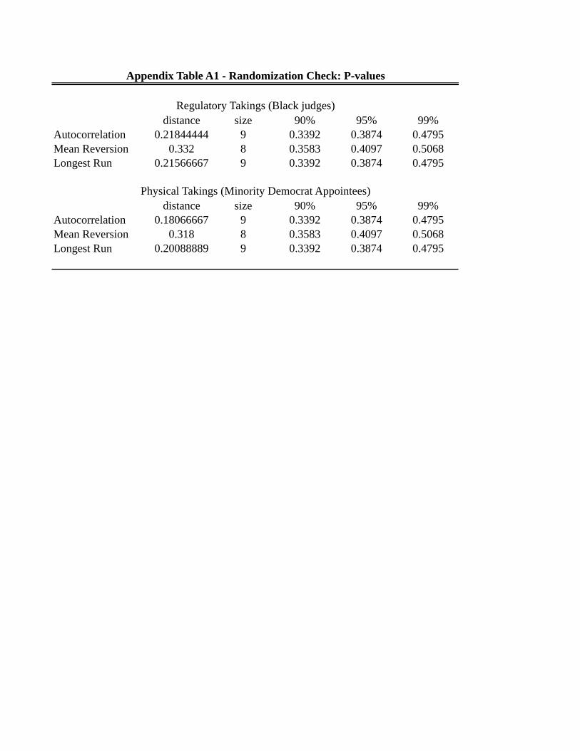
distance size 90% 95% 99%Autocorrelation 0.21844444 9 0.3392 0.3874 0.4795Mean Reversion 0.332 8 0.3583 0.4097 0.5068Longest Run 0.21566667 9 0.3392 0.3874 0.4795

distance size 90% 95% 99%Autocorrelation 0.18066667 9 0.3392 0.3874 0.4795Mean Reversion 0.318 8 0.3583 0.4097 0.5068Longest Run 0.20088889 9 0.3392 0.3874 0.4795

Regulatory Takings (Black judges)

Appendix Table A1 - Randomization Check: P-values

Physical Takings (Minority Democrat Appointees)

Circuit-Year Level(1) (2) (3) (4)

Black Judges per Seat, t 0.382* 0.418** 0.362* 0.340*(0.160) (0.129) (0.139) (0.140)

Black Judges per Seat, t-1 0.156 0.162(0.107) (0.104)

Black Judges per Seat, t-2 -0.154(0.234)

Black Judges per Seat, t+1 -0.244 -0.240(0.191) (0.189)

Black Judges per Seat, t+2 0.0836(0.107)

N 298 286 298 286R-sq 0.178 0.185 0.174 0.174

Appendix Table A2 -- Falsification Test of Instrument: Relationship Between Pro-Government Regulatory Takings Appellate Decisions and Composition of Regulatory Takings Panels in Other Years, 1979-2004

Outcome: Proportion of Pro-Takings Decisions, t

Notes: Heteroskedasticity-robust standard errors are in parentheses. Observations are clustered at the circuit level. Proportions of pro-takings decisions and judicial type per seat during circuit-years with no cases are defind to be 0 and dummied out. + Significant at 10%; * Significant at 5%; ** Significant at 1%

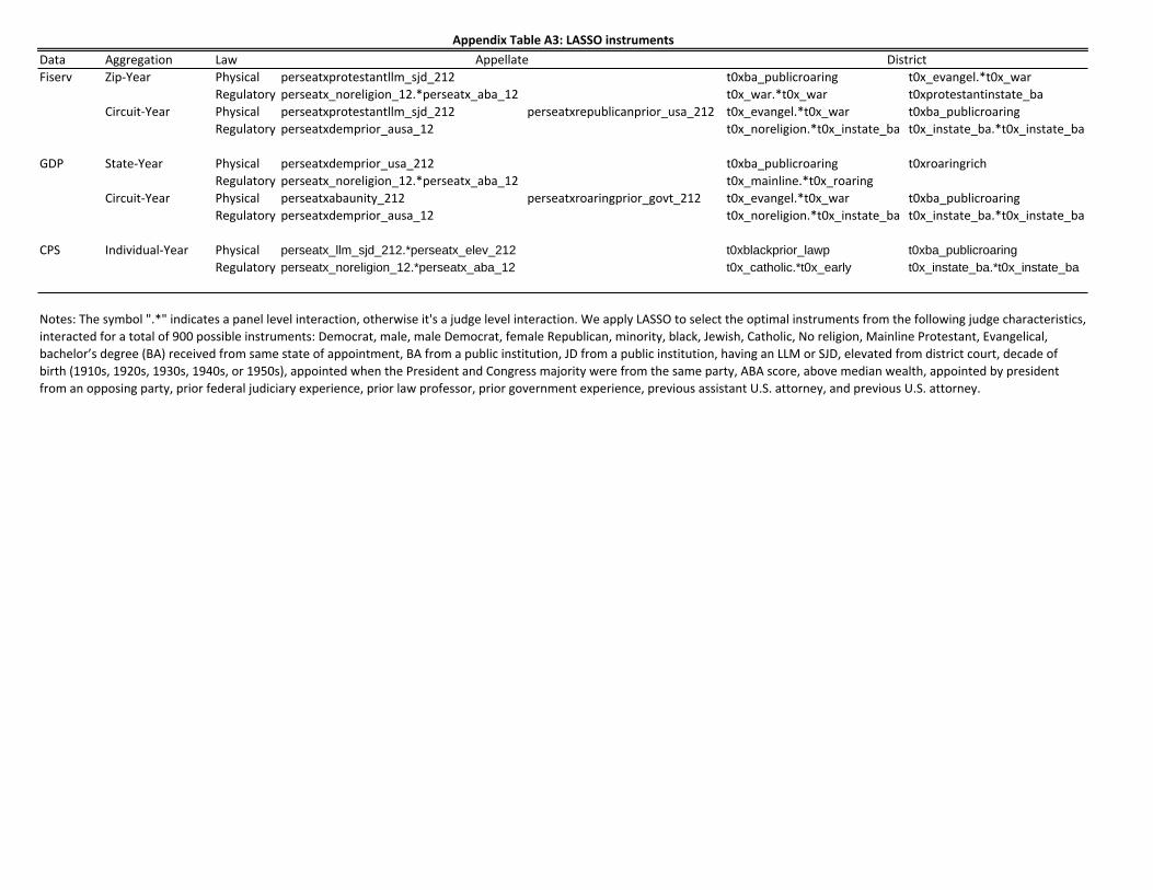
Data Aggregation Law

Fiserv Zip2Year Physical perseatxprotestantllm_sjd_212 t0xba_publicroaring t0x_evangel.*t0x_war

Regulatory perseatx_noreligion_12.*perseatx_aba_12 t0x_war.*t0x_war t0xprotestantinstate_ba

Circuit2Year Physical perseatxprotestantllm_sjd_212 perseatxrepublicanprior_usa_212 t0x_evangel.*t0x_war t0xba_publicroaring

Regulatory perseatxdemprior_ausa_12 t0x_noreligion.*t0x_instate_ba t0x_instate_ba.*t0x_instate_ba

GDP State2Year Physical perseatxdemprior_usa_212 t0xba_publicroaring t0xroaringrich

Regulatory perseatx_noreligion_12.*perseatx_aba_12 t0x_mainline.*t0x_roaring

Circuit2Year Physical perseatxabaunity_212 perseatxroaringprior_govt_212 t0x_evangel.*t0x_war t0xba_publicroaring

Regulatory perseatxdemprior_ausa_12 t0x_noreligion.*t0x_instate_ba t0x_instate_ba.*t0x_instate_ba

CPS Individual2Year Physical perseatx_llm_sjd_212.*perseatx_elev_212 t0xblackprior_lawp t0xba_publicroaringRegulatory perseatx_noreligion_12.*perseatx_aba_12 t0x_catholic.*t0x_early t0x_instate_ba.*t0x_instate_ba

Appendix(Table(A3:(LASSO(instrumentsAppellate District

Notes:LTheLsymbolL".*"LindicatesLaLpanelLlevelLinteraction,LotherwiseLit'sLaLjudgeLlevelLinteraction.LWeLapplyLLASSOLtoLselectLtheLoptimalLinstrumentsLfromLtheLfollowingLjudgeLcharacteristics,L

interactedLforLaLtotalLofL900LpossibleLinstruments:LDemocrat,Lmale,LmaleLDemocrat,LfemaleLRepublican,Lminority,Lblack,LJewish,LCatholic,LNoLreligion,LMainlineLProtestant,LEvangelical,L

bachelor’sLdegreeL(BA)LreceivedLfromLsameLstateLofLappointment,LBALfromLaLpublicLinstitution,LJDLfromLaLpublicLinstitution,LhavingLanLLLMLorLSJD,LelevatedLfromLdistrictLcourt,LdecadeLofL

birthL(1910s,L1920s,L1930s,L1940s,LorL1950s),LappointedLwhenLtheLPresidentLandLCongressLmajorityLwereLfromLtheLsameLparty,LABALscore,LaboveLmedianLwealth,LappointedLbyLpresidentL

fromLanLopposingLparty,LpriorLfederalLjudiciaryLexperience,LpriorLlawLprofessor,LpriorLgovernmentLexperience,LpreviousLassistantLU.S.Lattorney,LandLpreviousLU.S.Lattorney.

Average of yearly lags P-value of lags P-value of leads(1) (2) (3)

A. Add Circuit-Specific Trends 0.003 0.031 0.592

B. No Fixed Effects 0.006 0.721 0.942

C. State Cluster 0.005 0.012 0.843

D. Control for Expectation 0.007 0.000 0.576

E. Use Population Weights -0.004 0.054 0.244

F. Add 2-year Lead 0.008 0.005 0.032

G. Drop 1 Circuit Circuit 1 0.004 0.002 0.710 Circuit 2 0.003 0.391 0.552 Circuit 3 0.001 0.235 0.763 Circuit 4 0.007 0.003 0.742 Circuit 5 0.007 0.000 0.753 Circuit 6 0.004 0.446 0.217 Circuit 7 0.006 0.000 0.892 Circuit 8 -0.000 0.024 0.794 Circuit 9 0.014 0.001 0.858 Circuit 10 0.006 0.000 0.900 Circuit 11 0.002 0.133 0.883 Circuit 12 0.005 0.001 0.813

H. Circuit-quarter laws 0.013 0.000 0.658

The Effect of Appellate Regulatory Takings Precedent on ΔLog Price Index

Appendix Table A4 -- Impact of Regulatory Takings Precedent on House Prices -- Robustness of 2SLS Estimates

Notes: Significant at +10%, *5%, **1%. Data consist of Fiserv Case-Shiller/FHFA zip-code level price indices. Heteroskedasticity-robust standard errors are in parentheses and clustered by circuit. Regressions include circuit fixed effects, year and quarter fixed effects, and a dummy for whether there were no cases in that circuit-year. The baseline regression is an instrumental variables specification with one lead and four lags of appellate regulatory takings precedent, corresponding to column 2 in Table 5, Panel A. Instruments for appellate regulatory takings are Black judges per seat assigned to regulatory takings cases in a circuit-year. Expectation control is the expected probability of being assigned a Black judge per seat in a circuit-year. Population weights are based on the 2005 US Census estimates at the zip-code level.

(t0) (t1) (t2) (t3) (t4) (t5)A. Add Circuit-Specific Trends -0.008 0.005 0.007 0.013 -0.000

(0.010) (0.013) (0.007) (0.014) (0.008)B. No Fixed Effects -0.005 0.006 0.010 0.016 0.003

(0.018) (0.031) (0.029) (0.034) (0.009)C. State Cluster -0.011 0.004 0.011 0.017 0.005

(0.010) (0.014) (0.009) (0.012) (0.006)D. Control for Expectation -0.010 0.003 0.014 0.018 0.012

(0.014) (0.014) (0.009) (0.015) (0.013)E. Use Population Weights -0.019 -0.011 0.004 0.002 0.006

(0.016) (0.018) (0.015) (0.014) (0.007)F. Drop 1 Circuit

Drop Circuit 1 -0.011 0.003 0.010 0.015 0.005 (0.010) (0.012) (0.010) (0.014) (0.008)Drop Circuit 2 -0.014 0.002 0.007 0.015 0.004 (0.012) (0.016) (0.010) (0.015) (0.011)Drop Circuit 3 -0.008 0.003 0.004 0.007 -0.002 (0.012) (0.021) (0.018) (0.018) (0.008)Drop Circuit 4 -0.010 0.014 0.010 0.022 -0.001 (0.019) (0.030) (0.015) (0.027) (0.022)Drop Circuit 5 -0.008 0.006 0.013 0.017 0.006 (0.012) (0.013) (0.009) (0.013) (0.008)Drop Circuit 6 -0.011 0.002 0.009 0.010 0.011 (0.012) (0.009) (0.010) (0.014) (0.010)Drop Circuit 7 -0.009 0.006 0.012 0.015 0.005 (0.012) (0.012) (0.008) (0.013) (0.008)Drop Circuit 8 -0.012 -0.001 0.009 0.006 -0.004 (0.010) (0.009) (0.012) (0.014) (0.006)Drop Circuit 9 -0.008 0.019 0.020 0.034 0.003 (0.030) (0.028) (0.017) (0.029) (0.024)Drop Circuit 10 -0.011 0.007 0.012 0.019 0.004 (0.014) (0.016) (0.009) (0.018) (0.012)Drop Circuit 11 -0.023 0.003 0.003 0.029 -0.002 (0.018) (0.026) (0.010) (0.036) (0.033)Drop Circuit 12 -0.011 0.004 0.011 0.017 0.005 (0.012) (0.013) (0.010) (0.016) (0.009)

G. Lag Structure 1 Lag -0.001 0.004 (0.014) (0.007) 2 Lags -0.001 0.008 0.008 (0.016) (0.011) (0.008) 2 Leads, 4 Lags -0.007 0.001 0.019 0.013 0.014 (0.012) (0.014) (0.014) (0.014) (0.013) 1 Lead, 5 Lags -0.010+ 0.003 0.003 0.020 0.004 0.014 (0.005) (0.015) (0.015) (0.019) (0.009) (0.016) 4 Leads, 1 Lag 0.002 0.010 0.004 0.000 0.002 0.005 (t0, t1, f4, f3, f2, f1) (0.008) (0.015) (0.016) (0.017) (0.017) (0.007)

(q0) (q4) (q8) (q12) (q16) MeanH. Circuit-quarter laws 0.002 0.024 0.015 0.006 -0.0001 0.013

(0.020) (0.023) (0.031) (0.026) (0.011)I. Circuit-quarter laws (Lawct) -0.004 0.041 0.031 0.020 -0.011 0.026 controlling for (0.034) (0.027) (0.036) (0.044) (0.021)Local takings decision (LocalLawict) 0.093 0.021 -0.029 -0.148* -0.111 -0.054

(0.061) (0.062) (0.113) (0.066) (0.074)

Appendix Table A5 -- Impact of Regulatory Takings Precedent on House Prices

The Effect of Appellate Regulatory Takings Precedent on ΔLog Price Index

Notes: Significant at +10%, *5%, **1%. Data consist of Fiserv Case-Shiller/FHFA zip-code level price indices. Heteroskedasticity-robust standard errors are in parentheses and clustered by circuit. Regressions include circuit fixed effects, year and quarter fixed effects, and a dummy for whether there were no cases in that circuit-year. The baseline regression is an instrumental variables specification with one lead and four lags of appellate regulatory takings precedent, corresponding to column 2 in Table 5, Panel A. Coefficients on the lags are shown here. Instruments for appellate regulatory takings are Black judges per seat assigned to regulatory takings cases in a circuit-year. Expectation control is the expected probability of being assigned a Black judge per seat in a circuit-year. Population weights are based on the 2005 U.S. Census estimates at the zip-code level.

Robustness of 2SLS Distributed Lag Estimates

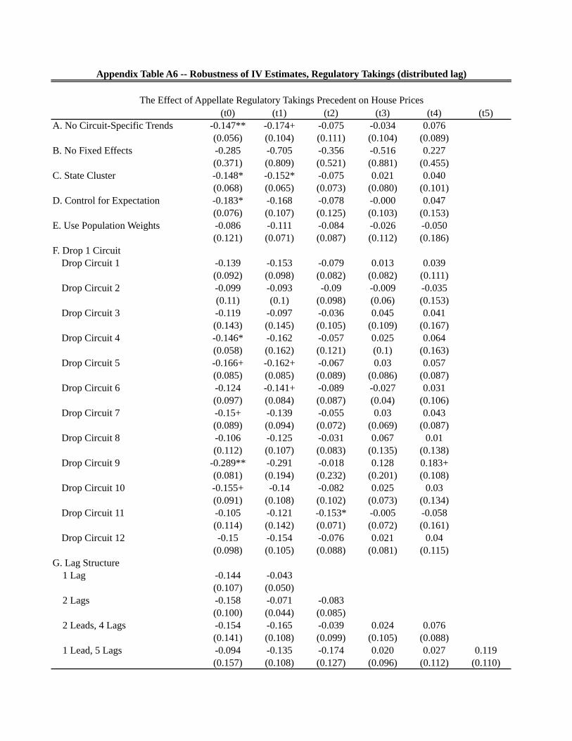
(t0) (t1) (t2) (t3) (t4) (t5)A. No Circuit-Specific Trends -0.147** -0.174+ -0.075 -0.034 0.076

(0.056) (0.104) (0.111) (0.104) (0.089)B. No Fixed Effects -0.285 -0.705 -0.356 -0.516 0.227

(0.371) (0.809) (0.521) (0.881) (0.455)C. State Cluster -0.148* -0.152* -0.075 0.021 0.040

(0.068) (0.065) (0.073) (0.080) (0.101)D. Control for Expectation -0.183* -0.168 -0.078 -0.000 0.047

(0.076) (0.107) (0.125) (0.103) (0.153)E. Use Population Weights -0.086 -0.111 -0.084 -0.026 -0.050

(0.121) (0.071) (0.087) (0.112) (0.186)F. Drop 1 Circuit

Drop Circuit 1 -0.139 -0.153 -0.079 0.013 0.039 (0.092) (0.098) (0.082) (0.082) (0.111)Drop Circuit 2 -0.099 -0.093 -0.09 -0.009 -0.035 (0.11) (0.1) (0.098) (0.06) (0.153)Drop Circuit 3 -0.119 -0.097 -0.036 0.045 0.041 (0.143) (0.145) (0.105) (0.109) (0.167)Drop Circuit 4 -0.146* -0.162 -0.057 0.025 0.064 (0.058) (0.162) (0.121) (0.1) (0.163)Drop Circuit 5 -0.166+ -0.162+ -0.067 0.03 0.057 (0.085) (0.085) (0.089) (0.086) (0.087)Drop Circuit 6 -0.124 -0.141+ -0.089 -0.027 0.031 (0.097) (0.084) (0.087) (0.04) (0.106)Drop Circuit 7 -0.15+ -0.139 -0.055 0.03 0.043 (0.089) (0.094) (0.072) (0.069) (0.087)Drop Circuit 8 -0.106 -0.125 -0.031 0.067 0.01 (0.112) (0.107) (0.083) (0.135) (0.138)Drop Circuit 9 -0.289** -0.291 -0.018 0.128 0.183+ (0.081) (0.194) (0.232) (0.201) (0.108)Drop Circuit 10 -0.155+ -0.14 -0.082 0.025 0.03 (0.091) (0.108) (0.102) (0.073) (0.134)Drop Circuit 11 -0.105 -0.121 -0.153* -0.005 -0.058 (0.114) (0.142) (0.071) (0.072) (0.161)Drop Circuit 12 -0.15 -0.154 -0.076 0.021 0.04 (0.098) (0.105) (0.088) (0.081) (0.115)

G. Lag Structure 1 Lag -0.144 -0.043 (0.107) (0.050) 2 Lags -0.158 -0.071 -0.083 (0.100) (0.044) (0.085) 2 Leads, 4 Lags -0.154 -0.165 -0.039 0.024 0.076 (0.141) (0.108) (0.099) (0.105) (0.088) 1 Lead, 5 Lags -0.094 -0.135 -0.174 0.020 0.027 0.119 (0.157) (0.108) (0.127) (0.096) (0.112) (0.110)

Appendix Table A6 -- Robustness of IV Estimates, Regulatory Takings (distributed lag)

The Effect of Appellate Regulatory Takings Precedent on House Prices

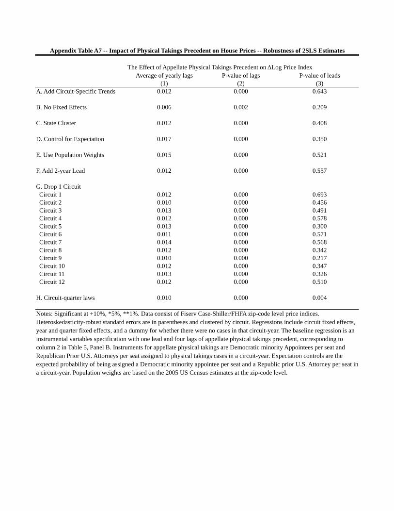
Average of yearly lags P-value of lags P-value of leads(1) (2) (3)

A. Add Circuit-Specific Trends 0.012 0.000 0.643

B. No Fixed Effects 0.006 0.002 0.209

C. State Cluster 0.012 0.000 0.408

D. Control for Expectation 0.017 0.000 0.350

E. Use Population Weights 0.015 0.000 0.521

F. Add 2-year Lead 0.012 0.000 0.557

G. Drop 1 Circuit Circuit 1 0.012 0.000 0.693 Circuit 2 0.010 0.000 0.456 Circuit 3 0.013 0.000 0.491 Circuit 4 0.012 0.000 0.578 Circuit 5 0.013 0.000 0.300 Circuit 6 0.011 0.000 0.571 Circuit 7 0.014 0.000 0.568 Circuit 8 0.012 0.000 0.342 Circuit 9 0.010 0.000 0.217 Circuit 10 0.012 0.000 0.347 Circuit 11 0.013 0.000 0.326 Circuit 12 0.012 0.000 0.510

H. Circuit-quarter laws 0.010 0.000 0.004

The Effect of Appellate Physical Takings Precedent on ΔLog Price Index

Appendix Table A7 -- Impact of Physical Takings Precedent on House Prices -- Robustness of 2SLS Estimates

Notes: Significant at +10%, *5%, **1%. Data consist of Fiserv Case-Shiller/FHFA zip-code level price indices. Heteroskedasticity-robust standard errors are in parentheses and clustered by circuit. Regressions include circuit fixed effects, year and quarter fixed effects, and a dummy for whether there were no cases in that circuit-year. The baseline regression is an instrumental variables specification with one lead and four lags of appellate physical takings precedent, corresponding to column 2 in Table 5, Panel B. Instruments for appellate physical takings are Democratic minority Appointees per seat and Republican Prior U.S. Attorneys per seat assigned to physical takings cases in a circuit-year. Expectation controls are the expected probability of being assigned a Democratic minority appointee per seat and a Republic prior U.S. Attorney per seat in a circuit-year. Population weights are based on the 2005 US Census estimates at the zip-code level.

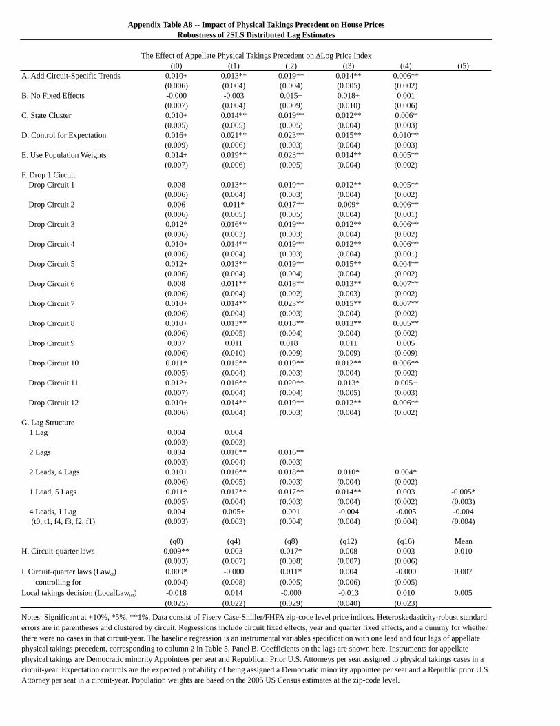
(t0) (t1) (t2) (t3) (t4) (t5)A. Add Circuit-Specific Trends 0.010+ 0.013** 0.019** 0.014** 0.006**

(0.006) (0.004) (0.004) (0.005) (0.002)B. No Fixed Effects -0.000 -0.003 0.015+ 0.018+ 0.001

(0.007) (0.004) (0.009) (0.010) (0.006)C. State Cluster 0.010+ 0.014** 0.019** 0.012** 0.006*

(0.005) (0.005) (0.005) (0.004) (0.003)D. Control for Expectation 0.016+ 0.021** 0.023** 0.015** 0.010**

(0.009) (0.006) (0.003) (0.004) (0.003)E. Use Population Weights 0.014+ 0.019** 0.023** 0.014** 0.005**

(0.007) (0.006) (0.005) (0.004) (0.002)F. Drop 1 Circuit

Drop Circuit 1 0.008 0.013** 0.019** 0.012** 0.005** (0.006) (0.004) (0.003) (0.004) (0.002)Drop Circuit 2 0.006 0.011* 0.017** 0.009* 0.006** (0.006) (0.005) (0.005) (0.004) (0.001)Drop Circuit 3 0.012* 0.016** 0.019** 0.012** 0.006** (0.006) (0.003) (0.003) (0.004) (0.002)Drop Circuit 4 0.010+ 0.014** 0.019** 0.012** 0.006** (0.006) (0.004) (0.003) (0.004) (0.001)Drop Circuit 5 0.012+ 0.013** 0.019** 0.015** 0.004** (0.006) (0.004) (0.004) (0.004) (0.002)Drop Circuit 6 0.008 0.011** 0.018** 0.013** 0.007** (0.006) (0.004) (0.002) (0.003) (0.002)Drop Circuit 7 0.010+ 0.014** 0.023** 0.015** 0.007** (0.006) (0.004) (0.003) (0.004) (0.002)Drop Circuit 8 0.010+ 0.013** 0.018** 0.013** 0.005** (0.006) (0.005) (0.004) (0.004) (0.002)Drop Circuit 9 0.007 0.011 0.018+ 0.011 0.005 (0.006) (0.010) (0.009) (0.009) (0.009)Drop Circuit 10 0.011* 0.015** 0.019** 0.012** 0.006** (0.005) (0.004) (0.003) (0.004) (0.002)Drop Circuit 11 0.012+ 0.016** 0.020** 0.013* 0.005+ (0.007) (0.004) (0.004) (0.005) (0.003)Drop Circuit 12 0.010+ 0.014** 0.019** 0.012** 0.006** (0.006) (0.004) (0.003) (0.004) (0.002)

G. Lag Structure 1 Lag 0.004 0.004 (0.003) (0.003) 2 Lags 0.004 0.010** 0.016** (0.003) (0.004) (0.003) 2 Leads, 4 Lags 0.010+ 0.016** 0.018** 0.010* 0.004* (0.006) (0.005) (0.003) (0.004) (0.002) 1 Lead, 5 Lags 0.011* 0.012** 0.017** 0.014** 0.003 -0.005* (0.005) (0.004) (0.003) (0.004) (0.002) (0.003) 4 Leads, 1 Lag 0.004 0.005+ 0.001 -0.004 -0.005 -0.004 (t0, t1, f4, f3, f2, f1) (0.003) (0.003) (0.004) (0.004) (0.004) (0.004)

(q0) (q4) (q8) (q12) (q16) MeanH. Circuit-quarter laws 0.009** 0.003 0.017* 0.008 0.003 0.010

(0.003) (0.007) (0.008) (0.007) (0.006)I. Circuit-quarter laws (Lawct) 0.009* -0.000 0.011* 0.004 -0.000 0.007 controlling for (0.004) (0.008) (0.005) (0.006) (0.005)Local takings decision (LocalLawict) -0.018 0.014 -0.000 -0.013 0.010 0.005

(0.025) (0.022) (0.029) (0.040) (0.023)

Appendix Table A8 -- Impact of Physical Takings Precedent on House Prices

The Effect of Appellate Physical Takings Precedent on ΔLog Price Index

Notes: Significant at +10%, *5%, **1%. Data consist of Fiserv Case-Shiller/FHFA zip-code level price indices. Heteroskedasticity-robust standard errors are in parentheses and clustered by circuit. Regressions include circuit fixed effects, year and quarter fixed effects, and a dummy for whether there were no cases in that circuit-year. The baseline regression is an instrumental variables specification with one lead and four lags of appellate physical takings precedent, corresponding to column 2 in Table 5, Panel B. Coefficients on the lags are shown here. Instruments for appellate physical takings are Democratic minority Appointees per seat and Republican Prior U.S. Attorneys per seat assigned to physical takings cases in a circuit-year. Expectation controls are the expected probability of being assigned a Democratic minority appointee per seat and a Republic prior U.S. Attorney per seat in a circuit-year. Population weights are based on the 2005 US Census estimates at the zip-code level.

Robustness of 2SLS Distributed Lag Estimates

Average of yearly lags P-value of lags P-value of leads(1) (2) (3)

A. Add Circuit-Specific Trends 0.013 0.195 0.960

B. No Fixed Effects 0.022 0.005 0.967

C. State Cluster 0.016 0.048 0.735

D. Control for Expectation 0.017 0.036 0.428

E. Use Population Weights -0.007 0.000 0.854

G. Drop 1 Circuit Circuit 1 0.011 0.061 0.522 Circuit 2 0.013 0.058 0.747 Circuit 3 0.015 0.387 0.517 Circuit 4 0.024 0.245 0.916 Circuit 5 0.017 0.074 0.685 Circuit 6 0.013 0.293 0.525 Circuit 7 0.017 0.104 0.686 Circuit 8 0.010 0.067 0.883 Circuit 9 0.024 0.171 0.938 Circuit 10 0.019 0.266 0.803 Circuit 11 0.013 0.034 0.829 Circuit 12 0.014 0.000 0.376

The Effect of Appellate Regulatory Takings Precedent on ΔLog GDP

Appendix Table A9 -- Impact of Regulatory Takings Precedent on Growth -- Robustness of 2SLS Estimates

Notes: Significant at +10%, *5%, **1%. State-level GDP data are from the Bureau of Economic Analysis. Heteroskedasticity-robust standard errors are in parentheses and clustered by circuit. Regressions include circuit fixed effects, year and quarterfixed effects, and a dummy for whether there were no cases in that circuit-year. The baseline regression is an instrumentalvariables specification with one lead and four lags of appellate regulatory takings precedent, corresponding to column 2 inTable 10, Panel A. Instruments for appellate regulatory takings are Black judges per seat assigned to appellate regulatorytakings cases in a circuit-year. Expectation control is the expected probability of being assigned a Black judge per seat in acircuit-year. Population weights are based on the 2005 US Census estimates at the zip-code level.

(t0) (t1) (t2) (t3) (t4) (t5)A. Add Circuit-Specific Trends -0.004 0.003 0.032+ -0.001 0.034+

(0.019) (0.010) (0.017) (0.015) (0.018)B. No Fixed Effects 0.015 -0.010 0.054 0.019 0.033

(0.026) (0.033) (0.042) (0.043) (0.039)C. State Cluster -0.010 0.002 0.040* 0.006 0.042*

(0.018) (0.016) (0.015) (0.015) (0.021)D. Control for Expectation -0.017 -0.003 0.043* 0.007 0.054

(0.026) (0.018) (0.022) (0.024) (0.034)E. Use Population Weights -0.047* -0.033* 0.007 0.003 0.034*

(0.020) (0.014) (0.022) (0.032) (0.014)F. Drop 1 Circuit

Drop Circuit 1 -0.020 -0.000 0.034* 0.004 0.037+ (0.018) (0.010) (0.015) (0.022) (0.022)Drop Circuit 2 -0.009 -0.000 0.030+ 0.010 0.036 (0.023) (0.012) (0.018) (0.018) (0.025)Drop Circuit 3 -0.009 0.005 0.044 0.002 0.032 (0.026) (0.016) (0.029) (0.026) (0.031)Drop Circuit 4 0.009 0.009 0.049+ 0.012 0.044 (0.022) (0.020) (0.029) (0.022) (0.034)Drop Circuit 5 -0.007 0.005 0.043* 0.003 0.042+ (0.023) (0.014) (0.019) (0.019) (0.023)Drop Circuit 6 -0.010 0.012 0.040 -0.011 0.037 (0.032) (0.015) (0.025) (0.022) (0.028)Drop Circuit 7 -0.008 0.006 0.041* 0.005 0.040+ (0.023) (0.011) (0.019) (0.021) (0.023)Drop Circuit 8 -0.012 0.005 0.030* 0.001 0.023+ (0.019) (0.010) (0.015) (0.020) (0.013)Drop Circuit 9 -0.013 -0.017 0.055+ 0.033 0.064 (0.033) (0.043) (0.033) (0.030) (0.055)Drop Circuit 10 -0.006 -0.001 0.037 0.007 0.056+ (0.027) (0.017) (0.023) (0.021) (0.029)Drop Circuit 11 -0.019 -0.004 0.037+ -0.000 0.053 (0.023) (0.022) (0.021) (0.027) (0.040)Drop Circuit 12 -0.022 0.001 0.035+ 0.009 0.047* (0.021) (0.015) (0.020) (0.024) (0.024)

G. Lag Structure 1 Lag 0.011 0.012 (0.022) (0.010) 2 Lags -0.000 0.032* 0.032+ (0.025) (0.013) (0.019) 2 Leads, 4 Lags -0.002 0.006 0.051 0.001 0.051+ (0.026) (0.023) (0.031) (0.024) (0.028) 1 Lead, 5 Lags -0.014 0.006 0.045 0.003 0.026 -0.019

(0.024) (0.010) (0.029) (0.015) (0.019) (0.022) 4 Leads, 1 Lag 0.027 0.012 -0.003 0.008 0.015 0.002 (t0, t1, f4, f3, f2, f1) (0.017) (0.020) (0.031) (0.019) (0.026) (0.021)

Appendix Table A10 -- Impact of Regulatory Takings Precedent on Growth

The Effect of Appellate Regulatory Takings Precedent on ΔLog GDP

Notes: Significant at +10%, *5%, **1%. State-level GDP data are from the Bureau of Economic Analysis.Heteroskedasticity-robust standard errors are in parentheses and clustered by circuit. Regressions include circuit fixedeffects, year and quarter fixed effects, and a dummy for whether there were no cases in that circuit-year. The baselineregression is an instrumental variables specification with one lead and four lags of appellate regulatory takingsprecedent, corresponding to column 2 in Table 10, Panel A. Coefficients on the lags are shown here. Instruments forappellate regulatory takings are Black judges per seat assigned to appellate regulatory takings cases in a circuit-year.Expectation control is the expected probability of being assigned a Black judge per seat in a circuit-year. Populationweights are based on the 2005 US Census estimates at the zip-code level.

Robustness of 2SLS Distributed Lag Estimates

Average of yearly lags P-value of lags P-value of leads(1) (2) (3)

A. Add Circuit-Specific Trends 0.008 0.011 0.894

B. No Fixed Effects 0.001 0.031 0.903

C. State Cluster 0.011 0.002 0.763

D. Control for Expectation 0.013 0.002 0.556

E. Use Population Weights 0.009 0.000 0.683

G. Drop 1 Circuit Circuit 1 0.010 0.001 0.767 Circuit 2 0.008 0.000 0.465 Circuit 3 0.012 0.000 0.601 Circuit 4 0.010 0.000 0.932 Circuit 5 0.011 0.001 0.644 Circuit 6 0.009 0.000 0.566 Circuit 7 0.008 0.004 0.759 Circuit 8 0.010 0.000 0.812 Circuit 9 0.025 0.000 0.451 Circuit 10 0.012 0.000 0.422 Circuit 11 0.011 0.000 0.740 Circuit 12 0.010 0.000 0.824

The Effect of Appellate Physical Takings Precedent on ΔLog GDP

Appendix Table A11 -- Impact of Physical Takings Precedent on Growth -- Robustness of 2SLS Estimates

Notes: Significant at +10%, *5%, **1%. State-level GDP data are from the Bureau of Economic Analysis. Heteroskedasticity-robust standard errors are in parentheses and clustered by circuit. Regressions include circuit fixed effects, year and quarterfixed effects, a dummy for whether there were no cases in that circuit-year. The baseline regression is an instrumental variablesspecification with one lead and four lags of appellate physical takings precedent, corresponding to column 2 in Table 10, PanelB. Instruments for appellate physical takings are Democratic minority Appointees per seat and Republican Prior US Attorneysper seat assigned to appellate physical takings cases in a circuit-year. Expectation controls are the expected probability ofbeing assigned a Democratic minority appointee per seat and a Republic prior U.S. Attorney per seat in a circuit-year.Population weights are based on the 2005 US Census estimates at the zip-code level.

(t0) (t1) (t2) (t3) (t4) (t5)A. Add Circuit-Specific Trends 0.002 0.015* 0.008+ 0.013+ 0.003

(0.008) (0.008) (0.004) (0.007) (0.009)B. No Fixed Effects -0.017 -0.005 0.019* 0.012 -0.004

(0.022) (0.006) (0.009) (0.015) (0.008)C. State Cluster 0.005 0.019* 0.010+ 0.014* 0.005

(0.009) (0.008) (0.005) (0.006) (0.007)D. Control for Expectation 0.006 0.023* 0.013** 0.015* 0.008

(0.012) (0.009) (0.005) (0.007) (0.011)E. Use Population Weights -0.001 0.014+ 0.016+ 0.015** 0.003

(0.008) (0.008) (0.009) (0.004) (0.007)F. Drop 1 Circuit

Drop Circuit 1 0.001 0.019* 0.010** 0.012* 0.005 (0.010) (0.009) (0.004) (0.006) (0.010)Drop Circuit 2 -0.002 0.019+ 0.011** 0.011** 0.003 (0.008) (0.010) (0.004) (0.004) (0.010)Drop Circuit 3 0.008 0.021* 0.010* 0.017* 0.004 (0.010) (0.009) (0.004) (0.007) (0.009)Drop Circuit 4 0.004 0.019* 0.009* 0.014* 0.005 (0.011) (0.009) (0.004) (0.006) (0.010)Drop Circuit 5 0.006 0.024** 0.008* 0.011+ 0.007 (0.009) (0.007) (0.004) (0.006) (0.009)Drop Circuit 6 0.002 0.019* 0.013** 0.012* 0.002 (0.010) (0.009) (0.004) (0.006) (0.009)Drop Circuit 7 0.004 0.011* 0.008+ 0.015* 0.003 (0.011) (0.005) (0.005) (0.007) (0.009)Drop Circuit 8 0.008 0.015+ 0.008+ 0.013+ 0.004 (0.009) (0.008) (0.005) (0.007) (0.009)Drop Circuit 9 0.010 0.021 0.033* 0.031 0.030** (0.016) (0.015) (0.015) (0.023) (0.009)Drop Circuit 10 0.006 0.020** 0.012** 0.014** 0.008 (0.008) (0.007) (0.004) (0.005) (0.008)Drop Circuit 11 0.006 0.021* 0.009* 0.014* 0.006 (0.010) (0.009) (0.004) (0.007) (0.010)Drop Circuit 12 0.003 0.020* 0.010** 0.014* 0.004 (0.010) (0.009) (0.004) (0.006) (0.009)

G. Lag Structure 1 Lag -0.003 0.007 (0.009) (0.007) 2 Lags -0.006 0.013* 0.009 (0.008) (0.006) (0.008) 2 Leads, 4 Lags 0.005 0.018+ 0.010* 0.014** 0.005 (0.010) (0.010) (0.005) (0.005) (0.009) 1 Lead, 5 Lags -0.000 0.020** 0.018** 0.017* 0.004 0.005

(0.008) (0.008) (0.004) (0.006) (0.009) (0.005) 4 Leads, 1 Lag -0.000 0.002 0.004 -0.018* 0.006 0.004 (t0, t1, f4, f3, f2, f1) (0.007) (0.006) (0.010) (0.009) (0.008) (0.009)

Appendix Table 12 -- Impact of Physical Takings Precedent on Growth

The Effect of Appellate Physical Takings Precedent on ΔLog GDP

Notes: Significant at +10%, *5%, **1%. State-level GDP data are from the Bureau of Economic Analysis.Heteroskedasticity-robust standard errors are in parentheses and clustered by circuit. Regressions include circuit fixedeffects, year and quarter fixed effects, and a dummy for whether there were no cases in that circuit-year. The baselineregression is an instrumental variables specification with one lead and four lags of appellate physical takings precedent,corresponding to column 2 in Table 10, Panel B. Coefficients on the lags are shown here. Instruments for appellatephysical takings are Democratic minority Appointees per seat and Republican Prior US Attorneys per seat assigned toappellate physical takings cases in a circuit-year. Expectation controls are the expected probability of being assigned aDemocratic minority appointee per seat and a Republic prior U.S. Attorney per seat in a circuit-year. Populationweights are based on the 2005 US Census estimates at the zip-code level.

Robustness of 2SLS Distributed Lag Estimates

Dependent Variable(1) (2) (3) (4) (5) (6) (7) (8) (9) (10) (11) (12)

Proportion Pro-Taking 0.00309 -0.0231 -0.000434 -0.000965 -0.00113 0.00621 0.00141 0.00409 0.00379 -0.0132 0.0102 0.0168 Appellate Decisionst+1 (0.00352) (0.0312) (0.0250) (0.0192) (0.000915) (0.00965) (0.00585) (0.00795) (0.00260) (0.0101) (0.0152) (0.0182)Proportion Pro-Taking 0.00540* -0.0136 0.00763 -0.00638 -0.00177+ -0.00196 -0.00675 0.00742 -0.000802 0.0110 0.00904 0.00462 Appellate Decisionst (0.00241) (0.0198) (0.0151) (0.0110) (0.000911) (0.00732) (0.00803) (0.00822) (0.00307) (0.0150) (0.0218) (0.0154)Proportion Pro-Taking 0.00685* -0.0192 0.00373 -0.0137 -0.000292 -0.00345 -0.00163 0.00890+ 0.000537 0.0181+ 0.00137 0.0129 Appellate Decisionst-1 (0.00287) (0.0210) (0.0177) (0.0124) (0.00112) (0.00484) (0.00614) (0.00466) (0.00346) (0.0104) (0.0130) (0.00854)Proportion Pro-Taking 0.00151 0.00748 -0.0221 -0.0184 -0.000534 -0.00368 -0.00362 0.00303 0.00196 -0.00852 -0.0240 0.00176 Appellate Decisionst-2 (0.00324) (0.0149) (0.0175) (0.0131) (0.000678) (0.00460) (0.00328) (0.00796) (0.00274) (0.0164) (0.0242) (0.0209)Proportion Pro-Taking -0.00269 -0.00252 0.000705 0.0159 -0.00175+ 0.00212 -0.000897 -0.0100 -0.000623 -0.00711 -0.0116 -0.0151 Appellate Decisionst-3 (0.00293) (0.0167) (0.0159) (0.0332) (0.000833) (0.00476) (0.00597) (0.0141) (0.00301) (0.0226) (0.0164) (0.0419)Proportion Pro-Taking -0.000317 0.00499 -0.0157 -0.0153 -0.000260 0.00385 0.00865 0.00706 -0.00287 0.00133 -0.00133 -0.0102 Appellate Decisionst-4 (0.00264) (0.0228) (0.0165) (0.0206) (0.00105) (0.00601) (0.00580) (0.00978) (0.00337) (0.0240) (0.0115) (0.0185)Proportion Pro-Takings -0.0182 0.00575 -0.0488 0.0802 0.00470 0.0186 0.0379 -0.0240 -0.000804 -0.0240 -0.0306 -0.146+ Appellate Decisionst+1 * Minority (0.0175) (0.0848) (0.0908) (0.0755) (0.00381) (0.0309) (0.0371) (0.0312) (0.0134) (0.0716) (0.0525) (0.0880)Proportion Pro-Takings -0.0228+ 0.0122 -0.166* -0.0408 0.0104* 0.0177 0.0319 0.00287 0.00679 -0.0751 0.0192 0.00374 Appellate Decisionst * Minority (0.0115) (0.0643) (0.0779) (0.0438) (0.00391) (0.0215) (0.0329) (0.0237) (0.0126) (0.0736) (0.0682) (0.0645)Proportion Pro-Takings -0.0348** -0.0379 0.00652 0.0186 0.0153+ 0.0259 0.0113 -0.0163 0.0231* 0.0000549 0.00262 -0.0343 Appellate Decisionst-1 * Minority (0.00955) (0.0485) (0.0605) (0.0308) (0.00781) (0.0211) (0.0228) (0.0141) (0.00882) (0.0385) (0.0244) (0.0276)Proportion Pro-Takings -0.0388** -0.0795+ 0.0666 -0.0282 0.0141* 0.0197 0.0171 0.00688 0.0284+ 0.119 0.110+ 0.110 Appellate Decisionst-2 * Minority (0.00893) (0.0481) (0.0612) (0.0839) (0.00594) (0.0310) (0.0270) (0.0337) (0.0135) (0.0853) (0.0644) (0.0868)Proportion Pro-Takings -0.0216* -0.0537 -0.0920 -0.115 0.00292 0.0274+ 0.0428 0.0552 0.0129 0.0866 0.00384 -0.0358 Appellate Decisionst-3 * Minority (0.00871) (0.0511) (0.0640) (0.175) (0.00269) (0.0162) (0.0271) (0.0742) (0.0132) (0.0646) (0.0473) (0.201)Proportion Pro-Takings -0.0117 -0.0157 0.00713 0.0181 0.00563 -0.0249 -0.0368* -0.00831 0.0190 -0.00143 0.0168 0.0981 Appellate Decisionst-4 * Minority (0.0117) (0.0498) (0.0788) (0.124) (0.00361) (0.0162) (0.0179) (0.0483) (0.0109) (0.0606) (0.0302) (0.125)Appellate IV N Y Y Lasso IV N Y Y Lasso IV N Y Y Lasso IVDistrict IV N N Lasso IV Lasso IV N N Lasso IV Lasso IV N N Lasso IV Lasso IVAggregation Level Individual Individual Individual Individual Individual Individual Individual Individual Individual Individual Individual IndividualN 3227637 3227637 3227637 3227637 3227637 3227637 3227637 3227637 3227637 3227637 3227637 3227637R-sq 0.065 0.065 0.062 0.063 0.024 0.022 0.019 0.020 0.043 0.041 0.041 0.034Mean dependent variable (Minority) 0.512 0.512 0.512 0.512 0.080 0.080 0.080 0.080 0.266 0.266 0.266 0.266Mean dependent variable (White) 0.714 0.714 0.714 0.714 0.017 0.017 0.017 0.017 0.119 0.119 0.119 0.119Average interaction lag -0.026 -0.035 -0.036 -0.029 0.010 0.013 0.013 0.008 0.018 0.026 0.031 0.028Average level effect lag 0.001 -0.003 -0.005 -0.002 -0.001 -0.000 -0.001 -0.001 0.000 0.002 -0.005 -0.007 P value of chi-sq of interaction lags 0.015 0.000 0.013 0.000 0.016 0.000 0.081 0.205 0.035 0.549 0.000 0.607 P value of chi-sq of level effect lags 0.126 0.307 0.733 0.000 0.114 0.733 0.010 0.000 0.244 0.299 0.222 0.279Average no appeal interaction lag -0.046 -0.048 -0.040 -0.084 0.015 0.011 0.005 0.027 0.040 0.043 0.041 0.071Average no appeal level effect lag 0.006 0.001 0.003 0.004 -0.001 -0.000 -0.000 -0.001 -0.004 -0.001 -0.013 -0.013 P value of no appeal interaction lags 0.000 0.000 0.095 0.000 0.000 0.000 0.427 0.000 0.000 0.000 0.001 0.002 P value no appeal level effect lags 0.060 0.861 0.483 0.932 0.012 0.871 0.214 0.532 0.051 0.512 0.000 0.198Typical Conditional interaction effect -0.0110 -0.0147 -0.0152 -0.0122 0.0042 0.0055 0.0055 0.0034 0.0076 0.0110 0.0131 0.0118 Conditional level effect 0.0004 -0.0013 -0.0021 -0.0008 -0.0004 0.0000 -0.0004 -0.0004 0.0000 0.0008 -0.0021 -0.0029 Unconditional interaction effect - pro 0.0070 0.0040 0.0004 0.0205 -0.0016 0.0012 0.0035 -0.0072 -0.0080 -0.0058 -0.0029 -0.0159 Unconditional interaction effect - anti 0.0064 0.0067 0.0056 0.0118 -0.0021 -0.0015 -0.0007 -0.0038 -0.0056 -0.0060 -0.0057 -0.0099 Unconditional interaction effect - all 0.0139 0.0112 0.0064 0.0331 -0.0039 -0.0005 0.0028 -0.0112 -0.0140 -0.0123 -0.0091 -0.0265

Appendix Table A13 - The Effect of Regulatory Takings Precedent on Housing InequalityLiving Below Poverty Line

Notes: Regressions of housing outcomes use March CPS. Heteroskedasticity-robust standard errors are in parentheses. Observations are clustered at the circuit level. Regressions include individual controls (age, race dummies, educational attainment dummies, and a marital status dummy), circuit fixed-effects, year fixed-effects, circuit-specific time trends, and a dummy for whether there were no cases in that circuit-year. Instruments for regulatory takings are Black judges per seat assigned to regulatory takings cases in a circuit-year. Instruments for physical takings are Democratic Nonwhite Appointees per seat and Republican Prior US Attorneys per seat assigned to physical takings cases in a circuit-year. LASSO Instruments are displayed in Appendix Table A3. Significant at +10%, *5%, **1%

Home Ownership Live in Public Housing

Dependent Variable(1) (2) (3) (4) (5) (6) (7) (8) (9) (10) (11) (12)

Proportion Pro-Taking 0.00131 -0.00879* -0.00915 0.00355 -0.00131 -0.00105 -0.00112 -0.00573 0.000634 0.00839* 0.00656 0.00602 Appellate Decisionst+1 (0.00338) (0.00377) (0.0137) (0.0150) (0.00106) (0.00214) (0.00208) (0.00527) (0.00416) (0.00409) (0.00437) (0.0112)Proportion Pro-Taking 0.0106** 0.0128+ 0.0204* 0.0257 -0.00147 -0.000193 -0.000831 -0.00145 -0.000716 0.00397 -0.00200 0.00530 Appellate Decisionst (0.00310) (0.00773) (0.00980) (0.0157) (0.00104) (0.00182) (0.00121) (0.00582) (0.00306) (0.00648) (0.00640) (0.0137)Proportion Pro-Taking 0.0131** 0.0121 0.0103* 0.00621 0.00123 0.00333 0.00242 0.00630+ -0.00111 -0.00331 -0.00521 0.00794 Appellate Decisionst-1 (0.00350) (0.00957) (0.00485) (0.0252) (0.00157) (0.00292) (0.00360) (0.00362) (0.00231) (0.00596) (0.00692) (0.0142)Proportion Pro-Taking 0.00435 -0.00353 -0.00395 0.0211 -0.00104 -0.000512 0.000278 0.000541 0.000334 0.000240 0.00215 -0.0137 Appellate Decisionst-2 (0.00400) (0.0101) (0.00984) (0.0293) (0.00103) (0.00348) (0.00202) (0.00518) (0.00204) (0.00460) (0.00238) (0.0253)Proportion Pro-Taking 0.000375 -0.00598 -0.000298 0.0125 -0.0000532 -0.000601 -0.00142 -0.00187 -0.00138 0.00947 0.00783 -0.00786 Appellate Decisionst-3 (0.00353) (0.0137) (0.00322) (0.0209) (0.00109) (0.00268) (0.00249) (0.00650) (0.00434) (0.00697) (0.00646) (0.0163)Proportion Pro-Taking 0.00397 0.00223 0.00313 0.0409* -0.000632 0.00205 0.000561 0.00856 -0.00524 0.00591 0.00127 -0.0280 Appellate Decisionst-4 (0.00354) (0.00950) (0.00999) (0.0184) (0.00132) (0.00239) (0.00287) (0.0108) (0.00399) (0.00822) (0.00870) (0.0314)Proportion Pro-Takings -0.0131 -0.0186 -0.00437 -0.0344 0.00230 0.00988 0.00575 0.00946 0.000825 0.000764 0.00460 0.0485 Appellate Decisionst+1 * Minority (0.0119) (0.0204) (0.0257) (0.0444) (0.00503) (0.00823) (0.00811) (0.0223) (0.00971) (0.0164) (0.0140) (0.0307)Proportion Pro-Takings -0.0386** -0.0586** -0.0540** -0.0823** 0.00583 0.00894* 0.00254 0.00283 0.00459 0.0245+ 0.0121 0.00872 Appellate Decisionst * Minority (0.0112) (0.0107) (0.0175) (0.0302) (0.00504) (0.00396) (0.00666) (0.0271) (0.00779) (0.0146) (0.0242) (0.0711)Proportion Pro-Takings -0.0289+ -0.00407 -0.0250* 0.0168 0.00909 0.000209 0.00811 -0.0256 0.00158 0.00166 0.0144 -0.117+ Appellate Decisionst-1 * Minority (0.0132) (0.0270) (0.0117) (0.105) (0.00819) (0.00468) (0.00964) (0.0264) (0.00930) (0.0118) (0.0110) (0.0621)Proportion Pro-Takings -0.0210 0.0113 0.0111 -0.00498 0.00971 0.00405 0.0121** 0.0287 0.00569 -0.00293 0.00114 0.0504 Appellate Decisionst-2 * Minority (0.0143) (0.0255) (0.0270) (0.111) (0.00549) (0.00390) (0.00367) (0.0358) (0.0132) (0.0168) (0.0149) (0.135)Proportion Pro-Takings -0.0328+ -0.0443 -0.0315 -0.0949 0.0102* 0.0104 -0.000374 0.0465 0.0287* 0.00874 0.00600 0.125 Appellate Decisionst-3 * Minority (0.0168) (0.0591) (0.0340) (0.130) (0.00371) (0.0118) (0.00580) (0.0388) (0.0130) (0.0203) (0.0150) (0.0992)Proportion Pro-Takings -0.0314+ -0.0292 -0.0298 -0.125 0.00865* 0.00359 -0.00764 -0.0239 0.0259+ -0.00175 -0.00128 0.00978 Appellate Decisionst-4 * Minority (0.0162) (0.0436) (0.0421) (0.0788) (0.00291) (0.00820) (0.0103) (0.0428) (0.0121) (0.0257) (0.0253) (0.121)Appellate IV N Y Y Lasso IV N Y Y Lasso IV N Y Y Lasso IVDistrict IV N N Lasso IV Lasso IV N N Lasso IV Lasso IV N N Lasso IV Lasso IVAggregation Level Individual Individual Individual Individual Individual Individual Individual Individual Individual Individual Individual IndividualN 4098609 4098609 4098609 4098609 4098609 4098609 4098609 4098609 4098609 4098609 4098609 4098609R-sq 0.062 0.062 0.062 0.060 0.024 0.024 0.023 0.022 0.041 0.041 0.041 0.038Mean dependent variable (Minority) 0.522 0.522 0.522 0.522 0.079 0.079 0.079 0.079 0.266 0.266 0.266 0.266Mean dependent variable (White) 0.721 0.721 0.721 0.721 0.017 0.017 0.017 0.017 0.117 0.117 0.117 0.117Average interaction lag -0.031 -0.025 -0.026 -0.058 0.009 0.005 0.003 0.006 0.013 0.006 0.006 0.015Average level effect lag 0.004 0.004 0.006 0.023 -0.001 0.000 0.000 0.001 -0.001 0.005 0.001 -0.010 P value of chi-sq of interaction lags 0.063 0.000 0.000 0.002 0.016 0.000 0.000 0.382 0.000 0.003 0.328 0.024 P value of chi-sq of level effect lags 0.020 0.111 0.000 0.000 0.002 0.647 0.534 0.032 0.076 0.020 0.001 0.573Average no appeal interaction lag -0.038 -0.038 -0.042 -0.033 0.014 0.013 0.016 0.016 0.033 0.034 0.034 0.032Average no appeal level effect lag 0.007 0.005 0.012 0.009 -0.001 -0.000 -0.002 -0.002 -0.005 -0.003 -0.007 -0.006 P value of no appeal interaction lags 0.000 0.000 0.000 0.000 0.000 0.000 0.000 0.000 0.000 0.000 0.000 0.000 P value no appeal level effect lags 0.014 0.229 0.005 0.002 0.006 0.101 0.346 0.004 0.003 0.000 0.000 0.381Typical Conditional interaction effect -0.0055 -0.0045 -0.0046 -0.0103 0.0016 0.0009 0.0005 0.0011 0.0023 0.0011 0.0011 0.0027 Conditional level effect 0.0007 0.0007 0.0011 0.0041 -0.0002 0.0000 0.0000 0.0002 -0.0002 0.0009 0.0002 -0.0018 Unconditional interaction effect - pro 0.0006 0.0016 0.0021 -0.0051 -0.0006 -0.0012 -0.0020 -0.0015 -0.0030 -0.0044 -0.0044 -0.0024 Unconditional interaction effect - anti 0.0030 0.0030 0.0034 0.0026 -0.0011 -0.0010 -0.0013 -0.0013 -0.0026 -0.0027 -0.0027 -0.0026 Unconditional interaction effect - all 0.0047 0.0058 0.0067 -0.0014 -0.0022 -0.0026 -0.0038 -0.0033 -0.0066 -0.0081 -0.0081 -0.0060

Appendix Table A14 - The Effect of Physical Takings Precedent on Housing InequalityHome Ownership Live in Public Housing Living Below Poverty Line

Notes: Regressions of housing outcomes use March CPS. Heteroskedasticity-robust standard errors are in parentheses. Observations are clustered at the circuit level. Regressions include individual controls (age, race dummies, educational attainment dummies, and a marital status dummy), circuit fixed-effects, year fixed-effects, circuit-specific time trends, and a dummy for whether there were no cases in that circuit-year. Instruments for regulatory takings are Black judges per seat assigned to regulatory takings cases in a circuit-year. Instruments for physical takings are Democratic Nonwhite Appointees per seat and Republican Prior US Attorneys per seat assigned to physical takings cases in a circuit-year. LASSO Instruments are displayed in Appendix Table A3. Significant at +10%, *5%, **1%

Dependent Variable(1) (2) (3) (4) (5) (6) (7) (8) (9) (10) (11) (12)

Proportion Pro-Taking -0.00111 0.0398 0.0193 0.0190* -0.171 1.352 0.387 0.778 -0.0154 0.193 0.111 0.103 Appellate Decisionst+1 (0.00243) (0.0345) (0.0336) (0.00910) (0.114) (1.446) (1.403) (0.548) (0.0166) (0.180) (0.195) (0.0678)Proportion Pro-Taking -0.00205 0.00842 -0.0000714 -0.00930 -0.196+ -0.224 -0.497 -0.824 -0.0192 0.0125 0.00101 -0.0496 Appellate Decisionst (0.00209) (0.0207) (0.0114) (0.0207) (0.103) (0.745) (0.424) (1.053) (0.0134) (0.116) (0.0657) (0.121)Proportion Pro-Taking -0.000683 0.0170 0.0121 0.00831 -0.0972 0.501 0.464 0.355 -0.0107 0.0520 0.0503 0.0396 Appellate Decisionst-1 (0.00281) (0.0223) (0.0114) (0.00974) (0.119) (1.036) (0.720) (0.585) (0.0155) (0.127) (0.0673) (0.0659)Proportion Pro-Taking 0.000887 0.0290+ 0.00325 -0.0146 -0.0349 1.187+ 0.457 -1.088 -0.00249 0.134 0.0142 -0.0887 Appellate Decisionst-2 (0.00210) (0.0161) (0.0156) (0.0209) (0.0908) (0.713) (0.859) (0.940) (0.0118) (0.0988) (0.0806) (0.124)Proportion Pro-Taking 0.000540 0.0247 0.0183 0.0289 0.0330 1.451 1.103 1.756 0.00128 0.130 0.0881 0.195+ Appellate Decisionst-3 (0.00223) (0.0226) (0.0173) (0.0196) (0.115) (1.136) (0.786) (1.114) (0.0138) (0.143) (0.0881) (0.107)Proportion Pro-Taking 0.00210 0.00616 -0.00924 -0.0202 0.172 0.432 -0.0499 -0.843 0.0148 0.0379 -0.0393 -0.0998 Appellate Decisionst-4 (0.00244) (0.0215) (0.0232) (0.0304) (0.0967) (0.944) (0.949) (1.375) (0.0131) (0.127) (0.138) (0.165)Proportion Pro-Takings -0.0126 -0.0870 -0.0246 -0.0195 -0.301 -2.769 -0.248 -1.141 -0.0595 -0.377 -0.0785 -0.100 Appellate Decisionst+1 * Minority (0.00735) (0.103) (0.0476) (0.0274) (0.242) (4.176) (1.776) (1.589) (0.0393) (0.559) (0.255) (0.163)Proportion Pro-Takings -0.0163* -0.0677 -0.0366 0.0198 -0.481+ -2.079 -0.613 1.990 -0.0890* -0.321 -0.224 0.105 Appellate Decisionst * Minority (0.00691) (0.0534) (0.0547) (0.0361) (0.223) (2.217) (1.735) (2.099) (0.0333) (0.305) (0.291) (0.195)Proportion Pro-Takings -0.0153+ -0.0923 -0.0371 -0.0110 -0.492+ -3.608 -1.562 -0.385 -0.0826+ -0.472 -0.201 -0.0581 Appellate Decisionst-1 * Minority (0.00752) (0.0605) (0.0281) (0.0158) (0.266) (2.355) (1.198) (0.880) (0.0415) (0.335) (0.135) (0.0973)Proportion Pro-Takings -0.0101 -0.132+ -0.0213 0.0309 -0.240 -5.203 -1.488 2.405 -0.0594 -0.726 -0.113 0.153 Appellate Decisionst-2 * Minority (0.00597) (0.0798) (0.0346) (0.0474) (0.224) (3.441) (1.366) (2.528) (0.0377) (0.475) (0.195) (0.260)Proportion Pro-Takings -0.00622 -0.101 -0.0337 -0.0745 -0.124 -4.295 -1.385 -3.905 -0.0321 -0.570 -0.162 -0.416 Appellate Decisionst-3 * Minority (0.00653) (0.0906) (0.0345) (0.0759) (0.245) (3.774) (1.233) (3.628) (0.0404) (0.525) (0.184) (0.407)Proportion Pro-Takings -0.00795 -0.0178 0.0183 0.0557 -0.284 -1.397 0.438 3.255 -0.0566 -0.170 0.0633 0.279 Appellate Decisionst-4 * Minority (0.00774) (0.0511) (0.0298) (0.0819) (0.277) (2.203) (1.090) (4.134) (0.0468) (0.274) (0.191) (0.461)Appellate IV N Y Y Lasso IV N Y Y Lasso IV N Y Y Lasso IVDistrict IV N N Lasso IV Lasso IV N N Lasso IV Lasso IV N N Lasso IV Lasso IVAggregation Level Individual Individual Individual Individual Individual Individual Individual Individual Individual Individual Individual IndividualN 5341620 5341620 5341620 5341620 5171040 5171040 5171040 5171040 4892691 4892691 4892691 4892691R-sq 0.093 0.090 0.092 0.092 0.126 0.124 0.126 0.125 0.125 0.123 0.124 0.124Mean dependent variable (Minority) 0.660 0.660 0.660 0.660 25.085 25.085 25.085 25.085 3.817 3.817 3.817 3.817Mean dependent variable (White) 0.750 0.750 0.750 0.750 29.527 29.527 29.527 29.527 4.405 4.405 4.405 4.405Average interaction lag -0.011 -0.082 -0.022 0.004 -0.324 -3.316 -0.922 0.672 -0.064 -0.452 -0.127 0.013Average level effect lag 0.000 0.015 0.005 0.003 -0.039 0.525 0.295 0.151 -0.004 0.065 0.023 0.030 P value of chi-sq of interaction lags 0.169 0.331 0.137 0.958 0.263 0.425 0.086 0.918 0.002 0.410 0.043 0.951 P value of chi-sq of level effect lags 0.336 0.130 0.773 0.397 0.010 0.064 0.650 0.426 0.012 0.212 0.900 0.206Average no appeal interaction lag -0.015 -0.067 -0.010 -0.014 0.135 0.560 0.330 0.380 0.018 0.065 0.036 0.047Average no appeal level effect lag 0.003 0.014 0.004 0.007 -0.573 -2.771 -0.508 -0.328 0.001 0.195 0.089 0.493 P value of no appeal interaction lags 0.025 0.170 0.375 0.728 0.008 0.255 0.607 0.714 0.035 0.243 0.824 0.467 P value no appeal level effect lags 0.281 0.106 0.822 0.505 0.011 0.112 0.549 0.608 -0.095 -0.381 -0.070 -0.106Typical Conditional interaction effect -0.0046 -0.0345 -0.0093 0.0017 -0.1365 -1.3967 -0.3883 0.2830 -0.0270 -0.1904 -0.0535 0.0055 Conditional level effect 0.0000 0.0063 0.0021 0.0013 -0.0164 0.2211 0.1243 0.0636 -0.0017 0.0274 0.0097 0.0126 Unconditional interaction effect - pro 0.0012 -0.0084 -0.0054 0.0071 -0.1891 -1.6151 -0.5170 0.1348 -0.0340 -0.2157 -0.0675 -0.0129 Unconditional interaction effect - anti 0.0021 0.0094 0.0014 0.0020 -0.0189 -0.0784 -0.0462 -0.0532 -0.0025 -0.0091 -0.0050 -0.0066 Unconditional interaction effect - all 0.0035 0.0016 -0.0039 0.0092 -0.2094 -1.6991 -0.5665 0.0778 -0.0367 -0.2255 -0.0729 -0.0199

Appendix Table A15 - The Effect of Regulatory Takings Precedent on Employment InequalityLog Real Earnings

Notes: Regressions of employment outcomes use MORG CPS. Heteroskedasticity-robust standard errors are in parentheses. Observations are clustered at the circuit level. Regressions include individual controls (age, race dummies, educational attainment dummies, and a marital status dummy), circuit fixed-effects, year fixed-effects, circuit-specific time trends, and a dummy for whether there were no cases in that circuit-year. Instruments for regulatory takings are Black judges per seat assigned to regulatory takings cases in a circuit-year. Instruments for physical takings are Democratic Nonwhite Appointees per seat and Republican Prior US Attorneys per seat assigned to physical takings cases in a circuit-year. LASSO Instruments are displayed in Appendix Table A3. Significant at +10%, *5%, **1%

Hours WorkedEmployment Status

Dependent Variable(1) (2) (3) (4) (5) (6) (7) (8) (9) (10) (11) (12)

Proportion Pro-Taking 0.00438 0.00538 0.00236 -0.0148 0.155 0.176 0.0942 -0.743 0.0254 0.0324 0.0183 -0.0771 Appellate Decisionst+1 (0.00268) (0.00583) (0.00479) (0.0112) (0.151) (0.198) (0.177) (0.538) (0.0219) (0.0440) (0.0360) (0.0800)Proportion Pro-Taking 0.00476* 0.0111+ 0.0128** -0.00533 0.135 0.443 0.536** -0.398 0.0285* 0.0725+ 0.0888** -0.0188 Appellate Decisionst (0.00165) (0.00652) (0.00386) (0.0203) (0.0936) (0.336) (0.205) (0.961) (0.0129) (0.0437) (0.0251) (0.129)Proportion Pro-Taking 0.00433* 0.00369 0.00643 -0.00380 0.161 0.210 0.334 -0.173 0.0268+ 0.0288 0.0411 -0.00455 Appellate Decisionst-1 (0.00180) (0.00434) (0.00486) (0.0167) (0.116) (0.261) (0.260) (0.837) (0.0135) (0.0289) (0.0330) (0.107)Proportion Pro-Taking 0.00577* 0.00872* 0.00802 0.0187 0.226+ 0.375* 0.320 0.796 0.0324* 0.0392 0.0398 0.0983 Appellate Decisionst-2 (0.00202) (0.00395) (0.00555) (0.0152) (0.118) (0.154) (0.273) (0.637) (0.0145) (0.0265) (0.0368) (0.0884)Proportion Pro-Taking 0.00545* 0.0170+ 0.0136* 0.00171 0.207 0.656 0.539+ -0.00831 0.0369* 0.0911 0.0858* 0.0279 Appellate Decisionst-3 (0.00245) (0.00951) (0.00607) (0.0108) (0.126) (0.482) (0.320) (0.535) (0.0158) (0.0620) (0.0377) (0.0769)Proportion Pro-Taking 0.00440 0.0104 0.00930 0.0480* 0.209 0.364 0.386 2.199** 0.0373 0.0781 0.0709+ 0.313* Appellate Decisionst-4 (0.00338) (0.00868) (0.00650) (0.0191) (0.155) (0.405) (0.325) (0.839) (0.0219) (0.0532) (0.0422) (0.133)Proportion Pro-Takings -0.0187* -0.0299+ -0.0179 0.0137 -0.599* -1.193* -0.762+ 0.467 -0.102** -0.187+ -0.118 0.0486 Appellate Decisionst+1 * Minority (0.00610) (0.0163) (0.0111) (0.0371) (0.234) (0.572) (0.409) (1.653) (0.0320) (0.106) (0.0733) (0.201)Proportion Pro-Takings -0.0218** -0.0406* -0.0341* -0.00752 -0.654** -1.460* -1.167+ 0.158 -0.125** -0.248* -0.216* -0.0677 Appellate Decisionst * Minority (0.00605) (0.0192) (0.0150) (0.0227) (0.204) (0.676) (0.600) (0.979) (0.0331) (0.113) (0.0885) (0.143)Proportion Pro-Takings -0.0113 -0.0114 -0.0178 -0.0145 -0.278 -0.280 -0.568 0.0278 -0.0660+ -0.0721+ -0.115+ -0.0904 Appellate Decisionst-1 * Minority (0.00660) (0.00907) (0.0120) (0.0202) (0.241) (0.333) (0.417) (0.790) (0.0320) (0.0412) (0.0611) (0.131)Proportion Pro-Takings -0.0134* -0.00274 -0.00482 -0.0377 -0.367 0.0775 -0.0555 -1.574 -0.0801* -0.0181 -0.0482 -0.255 Appellate Decisionst-2 * Minority (0.00568) (0.00776) (0.00636) (0.0348) (0.214) (0.323) (0.250) (1.244) (0.0318) (0.0516) (0.0448) (0.222)Proportion Pro-Takings -0.0184* -0.0262 -0.0159 -0.0207 -0.595* -0.716 -0.417 -1.416 -0.112* -0.151 -0.109 -0.201 Appellate Decisionst-3 * Minority (0.00717) (0.0230) (0.0126) (0.0448) (0.269) (0.851) (0.485) (2.092) (0.0422) (0.143) (0.0784) (0.296)Proportion Pro-Takings -0.0102 -0.0230 -0.0128 -0.0913+ -0.376 -0.643 -0.269 -3.072 -0.0727+ -0.162 -0.0902 -0.536 Appellate Decisionst-4 * Minority (0.00632) (0.0202) (0.0224) (0.0555) (0.224) (0.711) (0.778) (2.862) (0.0351) (0.117) (0.131) (0.358)Appellate IV N Y Y Lasso IV N Y Y Lasso IV N Y Y Lasso IVDistrict IV N N Lasso IV Lasso IV N N Lasso IV Lasso IV N N Lasso IV Lasso IVAggregation Level Individual Individual Individual Individual Individual Individual Individual Individual Individual Individual Individual IndividualN 6720948 6720948 6720948 6720948 6497313 6497313 6497313 6497313 6154598 6154598 6154598 6154598R-sq 0.095 0.095 0.095 0.093 0.131 0.131 0.131 0.130 0.128 0.128 0.128 0.127Mean dependent variable (Minority) 0.655 0.655 0.655 0.655 24.837 24.837 24.837 24.837 3.792 3.792 3.792 3.792Mean dependent variable (White) 0.742 0.742 0.742 0.742 29.130 29.130 29.130 29.130 4.348 4.348 4.348 4.348Average interaction lag -0.015 -0.021 -0.017 -0.034 -0.454 -0.604 -0.495 -1.175 -0.091 -0.130 -0.116 -0.230Average level effect lag 0.005 0.012 0.010 0.013 0.186 0.456 0.423 0.516 0.032 0.071 0.065 0.090 P value of chi-sq of interaction lags 0.016 0.011 0.001 0.004 0.084 0.003 0.135 0.000 0.019 0.013 0.000 0.000 P value of chi-sq of level effect lags 0.158 0.000 0.000 0.032 0.512 0.008 0.031 0.036 0.342 0.681 0.000 0.004Average no appeal interaction lag -0.012 -0.017 -0.010 -0.003 -0.428 -0.551 -0.351 -0.093 -0.078 -0.107 -0.079 -0.043Average no appeal level effect lag 0.004 0.008 0.008 0.003 0.195 0.340 0.369 0.174 0.027 0.046 0.054 0.031 P value of no appeal interaction lags 0.009 0.002 0.003 0.000 0.056 0.000 0.000 0.003 0.033 0.000 0.001 0.000 P value no appeal level effect lags 0.489 0.000 0.147 0.746 0.085 0.000 0.463 0.541 0.513 0.198 0.017 0.506Typical Conditional interaction effect -0.0027 -0.0037 -0.0030 -0.0061 -0.0809 -0.1076 -0.0882 -0.2094 -0.0162 -0.0232 -0.0207 -0.0410 Conditional level effect 0.0009 0.0021 0.0018 0.0023 0.0331 0.0813 0.0754 0.0920 0.0057 0.0127 0.0116 0.0160 Unconditional interaction effect - pro -0.0008 -0.0010 -0.0014 -0.0056 -0.0124 -0.0195 -0.0320 -0.1945 -0.0037 -0.0060 -0.0080 -0.0341 Unconditional interaction effect - anti 0.0010 0.0014 0.0008 0.0002 0.0342 0.0441 0.0281 0.0074 0.0062 0.0086 0.0063 0.0034 Unconditional interaction effect - all 0.0006 0.0008 -0.0003 -0.0052 0.0347 0.0411 0.0066 -0.1843 0.0048 0.0057 0.0007 -0.0294

Appendix Table A16 - The Effect of Physical Takings Precedent on Employment InequalityEmployment Status Hours Worked Log Real Earnings

Notes: Regressions of employment outcomes use MORG CPS. Heteroskedasticity-robust standard errors are in parentheses. Observations are clustered at the circuit level. Regressions include individual controls (age, race dummies, educational attainment dummies, and a marital status dummy), circuit fixed-effects, year fixed-effects, circuit-specific time trends, and a dummy for whether there were no cases in that circuit-year. Instruments for regulatory takings are Black judges per seat assigned to regulatory takings cases in a circuit-year. Instruments for physical takings are Democratic Nonwhite Appointees per seat and Republican Prior US Attorneys per seat assigned to physical takings cases in a circuit-year. LASSO Instruments are displayed in Appendix Table A3. Significant at +10%, *5%, **1%

Proportion Pro-Regulatory Taking 2 years later 3 years later N

(1) (2) (3)Minority Democratic Appointee Above Expectation 0.487 0.0551 0.0523 114

(0.0387) (0.00264) (0.00388) Below Expectation 0.743 0.0615 0.0601 354

(0.0216) (0.00184) (0.00211)Difference -0.256 -0.00640 -0.00779

(0.0415) (0.00323) (0.00407)

Republican Prior-US Attorney Above Expectation 0.918 0.0617 0.0580 73

(0.0258) (0.00393) (0.00378) Below Expectation 0.621 0.0591 0.0575 417

(0.0221) (0.00164) (0.00213)Difference 0.297 0.00265 0.000531

(0.0540) (0.00419) (0.00537)

Standard errors in parentheses. Coefficients display group means.

ΔLog GDP

Appendix Table A17 -- Wald Estimate Illustration

Appendix Figure A1 – Map of Local Takings

Regulatory Takings

Physical Takings

Appendix Figure A2: Randomization Check

P-Values of Black judge strings P-Values of Non-White Democrat strings!

!

! !

!