THE ECONOMIC FUTURE OFNUCLEAR POWER

A Study Conducted at The University of Chicago

August 2004

TH

E E

CO

NO

MIC

FU

TU

RE

OF

NU

CL

EA

R P

OW

ER

August 2004

Disclaimer

Neither the United States Government nor any agency thereof, nor The University of Chicago, norany of their employees or officers, makes any warranty, express or implied, or assumes any legalliability or responsibility for the accuracy, completeness, or usefulness of any information, apparatus,product, or process disclosed, or represents that its use would not infringe privately owned rights.The views and opinions of document authors expressed herein do not necessarily state or reflectthose of the United States Government or any agency thereof, Argonne National Laboratory, or theinstitutional opinions of The University of Chicago.

THE ECONOMIC FUTURE OF NUCLEAR POWER

A Study Conducted at The University of Chicago

August 2004

iii

TABLE OF CONTENTS

PART ONE: ECONOMIC COMPETITIVENESS OF NUCLEAR ENERGY1. Levelized Costs of Baseload Alternatives.............................................................. 1-12. International Comparisons ..................................................................................... 2-13. Capital Costs .......................................................................................................... 3-14. Learning by Doing ................................................................................................. 4-15. Financing Issues ..................................................................................................... 5-1

PART TWO: OUTLOOK FOR NUCLEAR ENERGY’S COMPETITORS6. Gas and Coal Technologies.................................................................................... 6-17. Fuel Prices .............................................................................................................. 7-18. Environmental Policies .......................................................................................... 8-1

PART THREE: NUCLEAR ENERGY IN THE YEARS AHEAD9. Nuclear Energy Scenarios: 2015 ........................................................................... . 9-110. Nuclear Energy Scenarios: Beyond 2015............................................................... 10-1

APPENDIX: MAJOR ISSUES AFFECTING THE NUCLEAR POWER INDUSTRYIN THE U.S. ECONOMY

A1. Purpose and Organization of Study.............................................................. . A1-1A2. Electricity Futures: A Review of Previous Studies....................................... A2-1A3. Need for New Generating Capacity in the United States.............................. A3-1A4. Technologies for New Nuclear Facilities...................................................... A4-1A5. Nuclear Fuel Cycle and Waste Disposal ....................................................... A5-1A6. Nuclear Regulation........................................................................................ A6-1A7. Nonproliferation Goals.................................................................................. A7-1A8. Hydrogen....................................................................................................... A8-1A9. Energy Security ............................................................................................. A9-1

ACRONYMS ........................................................................................................................ACM-1

TABLESTable 1-1: Summary Worksheet for Busbar Cost Comparisons, $ per MWh,

with Capital Costs in $ per kW, 2003 Prices ....................................... 1-8Table 2-1: Percent Distribution of 1998 Electricity Generation Capacity

by Country............................................................................................ 2-5Table 2-2: Number of Generation Sources Providing over 5 Percent

of Total Electricity in 1998 .................................................................. 2-6Table 2-3: Projected Percent Distribution of 2010 Electricity Generation

by Country............................................................................................ 2-7Table 2-4: Deutsche Bank Busbar Costs, 75 Percent Capacity Factor,

40-Year Plant Life, $ per MWh, 2003 Prices....................................... 2-9Table 2-5: OECD Busbar Costs, 75 Percent Capacity Factor,

40-Year Plant Life, $ per MWh, 2003 Prices....................................... 2-10

iv

TABLES(contd.)Table 2-6: Finnish Busbar Costs, 75 Percent Capacity Factor,

40-Year Plant Life, $ per MWh, 2003 Prices....................................... 2-12Table 2-7: Years Elapsed from Construction Start to Commercial Operation

as of December 31, 2001...................................................................... 2-13Table 2-8: Estimated Construction Costs for Recently Built Nuclear Power

Plants, $ per kW, 2003 Prices .............................................................. 2-14Table 2-9: Comparison of French and U.S. Busbar Costs, 25-Year Plant Life,

Technology-Specific Capacity Factors, 10 Percent Discount Rate,$ per MWh, 2003 Prices....................................................................... 2-15

Table 3-1: Capital Cost Distribution for 1,144 MW Advanced Boiling WaterReactor (ABWR), Mature Design, Including Contingencies andOwner’s Costs ..................................................................................... 3-7

Table 3-2: Percentage Distribution of Overnight Capital Costs by Account, forAdvanced Boiling Water Reactor (ABWR), Mature Design............... 3-8

Table 3-3: Capital Cost Estimates: Advanced Boiling Water Reactor (ABWR),Mature Design, in Millions of 2001 Dollars. ....................................... 3-13

Table 3-4: Components of Overnight and Total Capital Cost: Comparison ofALWR from Scully Report and ABWR .............................................. 3-14

Table 3-5: Cost Shares of LCOE: Overnight Capital, Interest, O&M, andFuel for Alternative Nuclear and Fossil Technologies......................... 3-16

Table 3-6: Sensitivity of Overnight and Interest Cost Contributions to TotalCapital Cost: Varying Construction Time and Weighted AverageCost of Capital (WACC), for Advanced Boiling Water Reactor(ABWR) ............................................................................................... 3-17

Table 3-7: Uncertainties in Overnight Capital Costs, $ per kW, 2003 Prices ....... 3-19Table 4-1: Summary of Regression Analyses of Learning by Doing in

Nuclear Power Plant Construction ...................................................... 4-7Table 4-2: Zimmerman’s Learning Effects ........................................................... 4-10Table 4-3: Regulatory Effects................................................................................ 4-17Table 4-4: Economies of Scale .............................................................................. 4-20Table 4-5: Regional Cost Differences ................................................................... 4-23Table 4-6: Conditions Associated with Alternative Learning Rates ..................... 4-25Table 5-1: Parameter Values for No-Policy Nuclear LCOE Calculations ............ 5-17Table 5-2: Risk Premiums for Alternative Investment Losses and Loss

Probabilities, 1-ps ................................................................................. 5-20Table 5-3: First-Plant LCOEs for Three Reactor Costs, 5- and 7-Year

Construction Periods, $ per MWh, 2003 Prices ................................... 5-23Table 5-4: LCOEs for Pulverized Coal Plants, 85 Percent Capacity Factors,

Alternative Overnight Costs, Coal Prices and ConstructionPeriods, $ per MWh, 2003 Prices......................................................... 5-24

Table 5-5: LCOEs for Gas Turbine Combined Cycle Plants, 85 PercentCapacity Factors, Alternative Overnight Costs, Gas Pricesand Construction Periods, $ per MWh, 2003 Prices ............................ 5-25

Table 5-6: Effects of Capacity Factor, Construction Period, and Plant Life onFirst-Plant Nuclear LCOE for Three Reactor Costs, $ per MWh,2003 Prices ........................................................................................... 5-26

v

TABLES(contd.)Table 5-7: The Impact of Construction Delays on the First-Plant LCOE of a

$1,500 per kW Plant, $ per MWh, 2003 Prices.................................... 5-28Table 6-1: Cost Expectations for New Coal Plants in 2003 .................................. 6-6Table 6-2: Thermal Efficiency Effect on Fuel Cost of GTCC, $ per MWh,

2003 Prices ........................................................................................... 6-8Table 6-3: Cost Estimates for New Gas Plants...................................................... 6-9Table 6-4: Effect of Fuel Price on Gas LCOE, $ per MWh .................................. 6-10Table 6-5: Effect of Environmental Controls on 2020 Gas-Fired LCOE.............. 6-11Table 6-6: Cost Characteristics of Fossil-Fired Electricity Generation................. 6-12Table 7-1: Coal Price Projections .......................................................................... 7-5Table 7-2: Natural Gas Price Projections .............................................................. 7-10Table 7-3: Year When Production Centers Become Cost Justified....................... 7-11Table 7-4: Estimates of Uranium Resources ......................................................... 7-13Table 7-5: MESSAGE Forecasts of North American Gas Production.................. 7-15Table 8-1: Average Costs Across Studies: IGCC, PCC, and GTCC

(David 2000) ........................................................................................ 8-6Table 8-2: Ground Transportation Cost Estimates, by Plant Type, $ per MWh ... 8-7Table 8-3: Injection and Storage Cost Estimates, by Plant Type, $ per MWh...... 8-8Table 8-4: Summary of Components of Carbon Sequestration Cost,

$ per MWh .......................................................................................... 8-9Table 8-5: Costs of Carbon Control, $ per MWh ................................................. 8-10Table 9-1: LCOEs for a First Nuclear Plant, with No Policy Assistance,

7-Year Construction Time, 10 Percent Interest Rate on Debt,15 Percent Rate on Equity, 2003 Prices ............................................... 9-5

Table 9-2: LCOEs for Coal and Gas Generation, 7 Percent Interest Rate onDebt, 12 Percent Rate on Equity, 2003 Prices ..................................... 9-6

Table 9-3: Nuclear LCOEs with Loan Guarantees, $ per MWh, 2003 Prices....... 9-7Table 9-4: Nuclear LCOEs with Accelerated Depreciation Allowances,

$ per MWh, 2003 Prices....................................................................... 9-7Table 9-5: Nuclear LCOEs with Investment Tax Credits, $ per MWh,

2003 Prices ........................................................................................... 9-8Table 9-6: Nuclear LCOEs with Production Tax Credits, $18 per MWh,

8-Year Duration, $ per MWh, 2003 Prices ......................................... 9-9Table 9-7: Effects of Combined $18 per MWh 8-Year Production Tax Credits

and 20 Percent Investment Tax Credits on Nuclear Plants’ LCOEs,$ per MWh, 2003 Prices....................................................................... 9-11

Table 9-8: LCOE for Successive Nuclear Plants, First to Eighth Plants,Learning Effects and Payment of FOAKE Costs Only, $ per MWh,2003 Prices ........................................................................................... 9-13

Table 9-9: LCOE for Successive Nuclear Plants, First to Eighth Plants,$ per MWh, 2003 Prices....................................................................... 9-15

Table 9-10: LCOE for Successive Nuclear Plant First to Eighth Plants, withDebt Share Responding to Reduced Risk, $ per MWh, 2003 Prices ... 9-15

Table 9-11: Contributors to LCOE Cost Reduction for Fifth Plant: Learning,Reduced Construction Time, and Elimination of Risk Premium,$ per MWh, 2003 Prices....................................................................... 9-16

vi

TABLES(contd.)Table 9-12: Fossil Fuel Generation LCOEs with and without Greenhouse

Policies, $ per MWh, 2003 Prices ........................................................ 9-17Table A1-1: Shares of Total U.S. Electricity Generation, by Type of

Generation ............................................................................................ A1-1Table A2-1: Plant and Market Model Summary ...................................................... A2-16Table A3-1: Estimates of the Long-Run Own-Price Elasticity of Residential

Demand for Electricity ......................................................................... A3-9 Table A3-2: Comparison of Forecasts of Electricity Demand Growth through

2020, Percent per Year ......................................................................... A3-12Table A3-3: Estimations of Future Generating Capacity Needs .............................. A3-12Table A3-4: Years When New Capacity will be Needed, by NERC Region,

with High and Low Growth Rates of Electricity Demand .................. A3-14Table A4-1: Number and Power (in MW) of Reactors, by Type and Continent...... A4-7Table A4-2: Summary of New Reactor Designs ...................................................... A4-11Table A5-1: Components of Front-End Nuclear Fuel Costs, $ per kg U,

2003 Prices ........................................................................................... A5-4Table A5-2: Disposal Costs, $ per MWh, 2003 Prices............................................. A5-9Table A5-3: Fuel Cycle Cost Components under Direct Disposal,

$ per MWh, 2003 Prices....................................................................... A5-10Table A6-1: Comparison of One-Step and Two-Step Licensing.............................. A6-5Table A6-2: LCOEs for Eighth Nuclear Plants, with No Policy Assistance

Other than Improved Regulation, $ per MWh, 2003 Prices................. A6-8Table A7-1: International Comparison of Nuclear Waste Disposal Policies ........... A7-4Table A8-1: Current Costs of Honda, Toyota, and General Motors Fuel Cell

Vehicles, 2003 Prices ........................................................................... A8-6Table A9-1: Natural Gas Prices, Recent and Forecasts, $ per MMBtu,

in 2003 Prices ....................................................................................... A9-7Table A9-2: Correlation Coefficients between Natural Gas Prices (Yearly

Averages, 1994 to 2001, in 2003 $ per 107 Kilocalories) betweenthe United States and Various Countries.............................................. A9-14

Table A9-3: Sensitivity of Model Calculation of Nuclear Share of NewConstruction ......................................................................................... A9-21

FIGURESFigure 5-1: The Effect of Debt Term: First-Plant LCOEs for a $1,500 per kW,

AP1000, and $1,200 per kW Plant with Reduced ConstructionTime and Higher Debt Ratio, $ per MWh, 2003 Prices....................... 5-27

Figure 7-1: NEMS Projections for U.S. Coal Prices.7-4Figure 7-2: U.S. Lower 48 Average Natural Gas Wellhead Price .......................... 7-7Figure 7-3: Natural Gas Wellhead Price: Difference between Actual

and Forecast.......................................................................................... 7-7Figure 7-4: U.S. Average Price of Uranium ........................................................... 7-12Figure 8-1: Trends in SO2 Allowance Prices .......................................................... 8-12Figure A3-1: 10-Year Moving Average of Residential Demand Growth/

GDP Growth Ratio ............................................................................... A3-4Figure A3-2: 10-Year Moving Average of Commercial Demand Growth/

GDP Growth Gap ................................................................................. A3-5

vii

FIGURES (contd.)Figure A3-3: Ratio of Manufacturing Electricity Consumption to Manufacturing

Output over Time, in Logs ................................................................... A3-7Figure A3-4: Ratio of Industry Electricity Usage to Industry Quantity Index

(1987=100) ........................................................................................... A3-7Figure A5-1: The Nuclear Fuel Cycle........................................................................ A5-4Figure A9-1: U.S. Natural Gas Production and Imports, 1970-2003 ........................ A9-10Figure A9-2: Electric Utility Sector Gas Prices in the United States, OECD

Europe, Japan, and Taiwan, 1994-2002, in 2003 Dollars .................... A9-12Figure A9-3: Industrial Sector Gas Prices in the United States, OECD

Europe, Japan, and Taiwan, 1994-2002, in 2003 Dollars .................... A9-13Figure A9-4: Household Sector Gas Prices in the United States, OECD

Europe, Japan, and Taiwan, 1994-2002, in 2003 Dollars .................... A9-13Figure A9-5: Determination of Additions to Nuclear Capacity................................. A9-19

viii

Part One: Economic Competitiveness of Nuclear Energy

Any policies concerned with the future of nuclear power must funnel through theprice at which nuclear power will enter the marketplace, if nuclear power is to be viable. Thelevelized cost of electricity (LCOE), as the price at the busbar needed to cover the operatingplus annualized capital costs of nuclear power, must be competitive with prices of otherbaseload electricity. Part One attempts to develop the most reliable estimates possible of thefuture busbar cost of nuclear electricity.

A starting point is estimates of nuclear generator costs from previous studies. Theseestimates for the United States are reviewed in Chapter 1. Chapter 2 is a parallelinternational review.

In light of the importance of capital costs and the role they have played incontributing to differences in LCOE estimates, Chapter 3 is devoted to the anatomy of theestimation of capital costs. An aim is to narrow the range of uncertainty in estimates offuture capital costs. Chapter 4 proceeds to another major reason for uncertainty aboutnuclear costs, which is learning from experience in constructing facilities. Drawing onanalyses of earlier nuclear experience and innovations in manufacturing more generally,estimates are developed of the extent to which costs can be expected to fall between thebuilding of the first and nth plants of a given technology.

Chapter 5 develops the financial model used in this study to evaluate the prospects fornuclear power. The complications of the tax system and of private sector financing asinfluenced by risk are introduced. No-policy estimates of nuclear LCOEs are estimated to setthe stage for the later policy analysis.

1-1

Chapter 1. LEVELIZED COSTS OF BASELOAD ALTERNATIVES

Summary

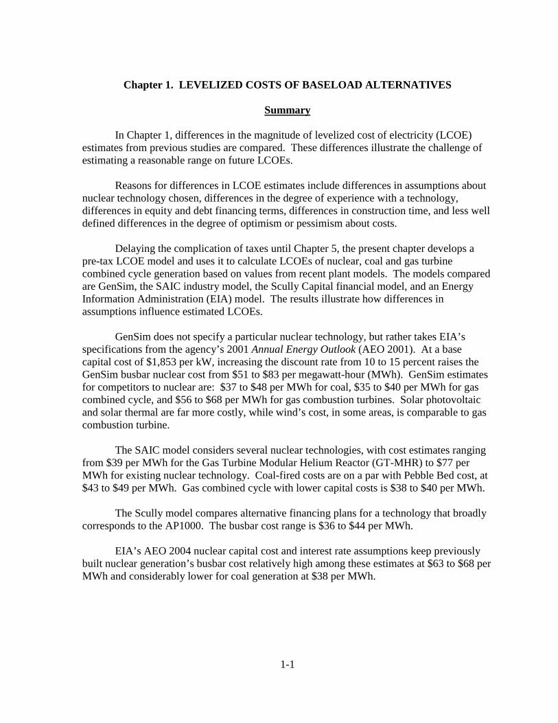
In Chapter 1, differences in the magnitude of levelized cost of electricity (LCOE)estimates from previous studies are compared. These differences illustrate the challenge ofestimating a reasonable range on future LCOEs.

Reasons for differences in LCOE estimates include differences in assumptions aboutnuclear technology chosen, differences in the degree of experience with a technology,differences in equity and debt financing terms, differences in construction time, and less welldefined differences in the degree of optimism or pessimism about costs.

Delaying the complication of taxes until Chapter 5, the present chapter develops apre-tax LCOE model and uses it to calculate LCOEs of nuclear, coal and gas turbinecombined cycle generation based on values from recent plant models. The models comparedare GenSim, the SAIC industry model, the Scully Capital financial model, and an EnergyInformation Administration (EIA) model. The results illustrate how differences inassumptions influence estimated LCOEs.

GenSim does not specify a particular nuclear technology, but rather takes EIA’sspecifications from the agency’s 2001 Annual Energy Outlook (AEO 2001). At a basecapital cost of $1,853 per kW, increasing the discount rate from 10 to 15 percent raises theGenSim busbar nuclear cost from $51 to $83 per megawatt-hour (MWh). GenSim estimatesfor competitors to nuclear are: $37 to $48 per MWh for coal, $35 to $40 per MWh for gascombined cycle, and $56 to $68 per MWh for gas combustion turbines. Solar photovoltaicand solar thermal are far more costly, while wind’s cost, in some areas, is comparable to gascombustion turbine.

The SAIC model considers several nuclear technologies, with cost estimates rangingfrom $39 per MWh for the Gas Turbine Modular Helium Reactor (GT-MHR) to $77 perMWh for existing nuclear technology. Coal-fired costs are on a par with Pebble Bed cost, at$43 to $49 per MWh. Gas combined cycle with lower capital costs is $38 to $40 per MWh.

The Scully model compares alternative financing plans for a technology that broadlycorresponds to the AP1000. The busbar cost range is $36 to $44 per MWh.

EIA’s AEO 2004 nuclear capital cost and interest rate assumptions keep previouslybuilt nuclear generation’s busbar cost relatively high among these estimates at $63 to $68 perMWh and considerably lower for coal generation at $38 per MWh.

1-2

Outline

1.1. Introduction

1.2. Representative Studies of Baseload Generation Costs

1.3. The LCOE Concept

1.4. A Pre-Tax LCOE Model

1.4.1. Capital Cost, K1.4.2. Insurance Cost, I1.4.3. Fixed O&M Cost, Mf

1.4.4. Variable O&M Cost, Mv

1.4.5. Fuel Cost, F1.4.6. Additional Factors

1.5. Before-Tax Comparisons of Busbar Costs of Nuclear, Coal, and Gas Generation in the United States

References

1-3

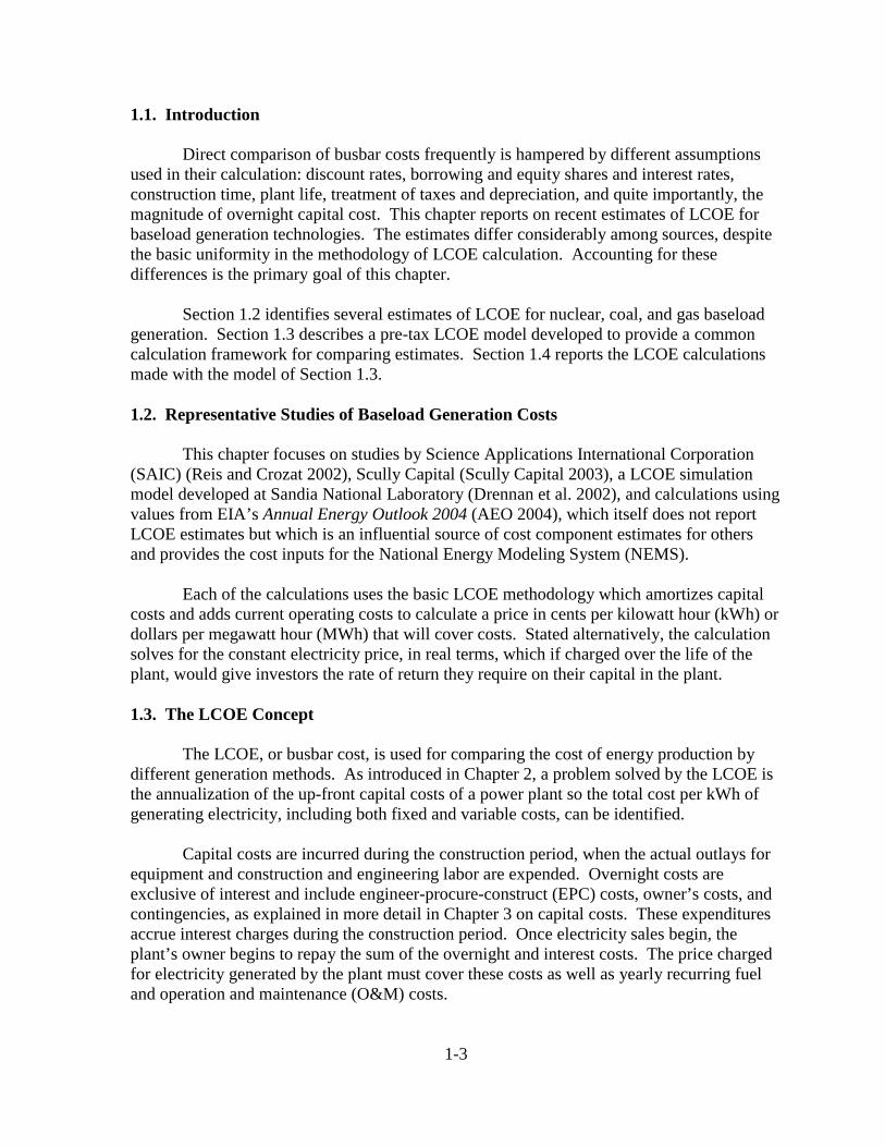
1.1. Introduction

Direct comparison of busbar costs frequently is hampered by different assumptionsused in their calculation: discount rates, borrowing and equity shares and interest rates,construction time, plant life, treatment of taxes and depreciation, and quite importantly, themagnitude of overnight capital cost. This chapter reports on recent estimates of LCOE forbaseload generation technologies. The estimates differ considerably among sources, despitethe basic uniformity in the methodology of LCOE calculation. Accounting for thesedifferences is the primary goal of this chapter.

Section 1.2 identifies several estimates of LCOE for nuclear, coal, and gas baseloadgeneration. Section 1.3 describes a pre-tax LCOE model developed to provide a commoncalculation framework for comparing estimates. Section 1.4 reports the LCOE calculationsmade with the model of Section 1.3.

1.2. Representative Studies of Baseload Generation Costs

This chapter focuses on studies by Science Applications International Corporation(SAIC) (Reis and Crozat 2002), Scully Capital (Scully Capital 2003), a LCOE simulationmodel developed at Sandia National Laboratory (Drennan et al. 2002), and calculations usingvalues from EIA’s Annual Energy Outlook 2004 (AEO 2004), which itself does not reportLCOE estimates but which is an influential source of cost component estimates for othersand provides the cost inputs for the National Energy Modeling System (NEMS).

Each of the calculations uses the basic LCOE methodology which amortizes capitalcosts and adds current operating costs to calculate a price in cents per kilowatt hour (kWh) ordollars per megawatt hour (MWh) that will cover costs. Stated alternatively, the calculationsolves for the constant electricity price, in real terms, which if charged over the life of theplant, would give investors the rate of return they require on their capital in the plant.

1.3. The LCOE Concept

The LCOE, or busbar cost, is used for comparing the cost of energy production bydifferent generation methods. As introduced in Chapter 2, a problem solved by the LCOE isthe annualization of the up-front capital costs of a power plant so the total cost per kWh ofgenerating electricity, including both fixed and variable costs, can be identified.

Capital costs are incurred during the construction period, when the actual outlays forequipment and construction and engineering labor are expended. Overnight costs areexclusive of interest and include engineer-procure-construct (EPC) costs, owner’s costs, andcontingencies, as explained in more detail in Chapter 3 on capital costs. These expendituresaccrue interest charges during the construction period. Once electricity sales begin, theplant’s owner begins to repay the sum of the overnight and interest costs. The price chargedfor electricity generated by the plant must cover these costs as well as yearly recurring fueland operation and maintenance (O&M) costs.

1-4

While there are many variants in implementing LCOE calculations, the basicframework remains largely the same. The greatest differences in the many applications lie intheir treatments of financing costs, inflation, and taxes, although additional costconsiderations can be implemented as well. Accounting for taxes in an LCOE modelintroduces a number of complications which are dealt with in Chapter 5 on financing.Inflation affects the nominal value of taxable income, as does the allocation of financingbetween debt and equity, since debt repayments are expenses deductible against taxableincome. Furthermore, without consideration of taxes, depreciation is immaterial.

1.4. A Pre-Tax LCOE Model

The LCOE model developed for this chapter contains five LCOE cost components:annuitized capital cost (A), insurance (I), fixed O&M costs (Mf), variable O&M costs (Mv),and fuel costs (F). The LCOE is such that a charge per kWh of this amount over the life ofthe plant will give present value of revenues just equal to the present value of the cost ofconstructing the plant and operating it over its life.

The revenue in any year is LCOE • W • 8760 • CFt, where W is the kW capacity of theplant, 8,760 is the number of hours in a year, and CFt is the fraction of capacity at which theplant is operated during the year (capacity factor). The present value of the revenues is thediscounted series of yearly revenues over the plant life:

PV(revenue)= ∑t

(LCOE • W • 8760 • CFt)/(1 + r)t ,

where r is the debt-and-equity-weighted average discount rate. The present value of costs is

,)1/()( tv

tf rFMMIK ++++= ∑

where K is the present value of the capital stock. Equating the present value of revenues andcosts and solving for the LCOE that brings about equality gives

,FMMIALCOE vf ++++=

where

])1/(8760/[ t

tt rCFWKA += ∑ .

1-5

1.4.1. Capital Cost, K

To obtain K, the total capital cost including financing is calculated by compoundingthe cost plus interest from the beginning of the construction until the plant is completed,using

,)1( 1+−+= ∑ tnn

tt rCPK

where

n = years required for constructionC = total overnight cost before financingPt = percentage of overnight cost outlay in year tr = weighted average of debt and equity interest rates.

1.4.2. Insurance Cost, I

Insurance cost is entered as an insurance rate that is a fraction of the capital cost. I =C • Insurance rate.

1.4.3. Fixed O&M Cost, Mf

Fixed O&M cost includes items from rent to workers’ wages. This cost is dependenton the size, rather than the output, of the plant. It is given as $ per kW. Fixed O&M cost iscalculated as

Mf = Fixed cost in $ per kW • plant size in kW • plant life.

1.4.4. Variable O&M Cost, Mv

Variable O&M is given in the form $ per kWh and is entered directly into the LCOEformula as Mv.

1.4.5. Fuel Cost, F

Fuel cost is calculated using the formula F • HR, where

F = Fuel cost in $ per MMBtu HR = Heat Rate in MMBtu.

1.4.6. Additional Factors

While this model incorporates the basic components of LCOE, it is not allencompassing, as it omits taxes and decommissioning and decontamination (D&D) cost.

1-6

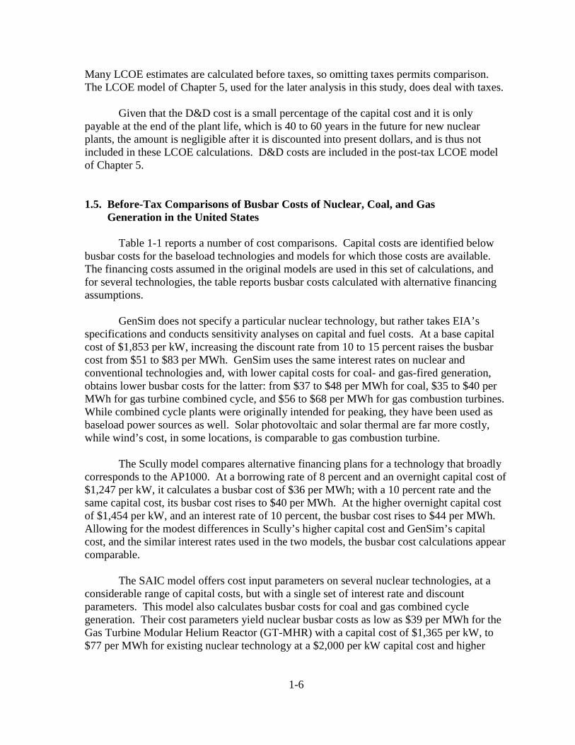
Many LCOE estimates are calculated before taxes, so omitting taxes permits comparison.The LCOE model of Chapter 5, used for the later analysis in this study, does deal with taxes.

Given that the D&D cost is a small percentage of the capital cost and it is onlypayable at the end of the plant life, which is 40 to 60 years in the future for new nuclearplants, the amount is negligible after it is discounted into present dollars, and is thus notincluded in these LCOE calculations. D&D costs are included in the post-tax LCOE modelof Chapter 5.

1.5. Before-Tax Comparisons of Busbar Costs of Nuclear, Coal, and Gas Generation in the United States

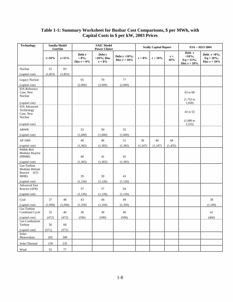
Table 1-1 reports a number of cost comparisons. Capital costs are identified belowbusbar costs for the baseload technologies and models for which those costs are available.The financing costs assumed in the original models are used in this set of calculations, andfor several technologies, the table reports busbar costs calculated with alternative financingassumptions.

GenSim does not specify a particular nuclear technology, but rather takes EIA’sspecifications and conducts sensitivity analyses on capital and fuel costs. At a base capitalcost of $1,853 per kW, increasing the discount rate from 10 to 15 percent raises the busbarcost from $51 to $83 per MWh. GenSim uses the same interest rates on nuclear andconventional technologies and, with lower capital costs for coal- and gas-fired generation,obtains lower busbar costs for the latter: from $37 to $48 per MWh for coal, $35 to $40 perMWh for gas turbine combined cycle, and $56 to $68 per MWh for gas combustion turbines.While combined cycle plants were originally intended for peaking, they have been used asbaseload power sources as well. Solar photovoltaic and solar thermal are far more costly,while wind’s cost, in some locations, is comparable to gas combustion turbine.

The Scully model compares alternative financing plans for a technology that broadlycorresponds to the AP1000. At a borrowing rate of 8 percent and an overnight capital cost of$1,247 per kW, it calculates a busbar cost of $36 per MWh; with a 10 percent rate and thesame capital cost, its busbar cost rises to $40 per MWh. At the higher overnight capital costof $1,454 per kW, and an interest rate of 10 percent, the busbar cost rises to $44 per MWh.Allowing for the modest differences in Scully’s higher capital cost and GenSim’s capitalcost, and the similar interest rates used in the two models, the busbar cost calculations appearcomparable.

The SAIC model offers cost input parameters on several nuclear technologies, at aconsiderable range of capital costs, but with a single set of interest rate and discountparameters. This model also calculates busbar costs for coal and gas combined cyclegeneration. Their cost parameters yield nuclear busbar costs as low as $39 per MWh for theGas Turbine Modular Helium Reactor (GT-MHR) with a capital cost of $1,365 per kW, to$77 per MWh for existing nuclear technology at a $2,000 per kW capital cost and higher

1-7

interest rates. SAIC’s coal-fired capital costs are on a par with Pebble Bed Modular Reactor(PBMR) capital cost, giving similar busbar costs, $43 to $49 per MWh. Gas turbinecombined cycle capital costs are projected much lower, and busbar costs are correspondinglylower, at $38 to $40 per MWh.

The latest Annual Energy Outlook (EIA 2004, pp. 5-58) reduces nuclear capital costassumptions below those in previous AEOs (EIA 2003, p. 73, Table 40). The two right-handcolumns of Table 1-1 use the new EIA nuclear capital cost estimates. The nuclear base casecapital cost estimate makes new nuclear generation’s busbar cost relatively high among theestimates in this table, at $63 to $68 per MWh for the nuclear base case, but lower for theadvanced nuclear case, at $43 to $53 per MWh. EIA’s estimate is considerably lower forcoal generation, at $38, and for gas generation, at $41.

1-8

Table 1-1: Summary Worksheet for Busbar Cost Comparisons, $ per MWh, withCapital Costs in $ per kW, 2003 Prices

Sandia ModelGenSim

SAIC ModelPower Choice Scully Capital Report EIA – AEO 2004 Technology

r=10% r=15%Debt r= 8%;

Disc r = 8%

Debt r=10%; Disc

r = 8%

Debt r =10%;Disc r = 10%

r = 8% r = 10% r =10%

Debt r=10%;

Eq = 15%;Disc r = 10%

Debt r =8%;Eq = 10%;

Disc r = 10%

Nuclear 51 83

(capital cost) (1,853) (1,853)

Legacy Nuclear 65 70 77

(capital cost) (2,000) (2,000) (2,000) EIA ReferenceCase, NewNuclear

63 to 68

(capital cost)(1,752 to

1,928)EIA AdvancedTechnologyCase, NewNuclear

43 to 53

(capital cost)(1,080 to

1,555)

ABWR 53 50 55

(capital cost) (1,600) (1,600) (1,600)

AP 1000 49 46 51 36 40 44

(capital cost) (1,365) (1,365) (1,365) (1,247) (1,247) (1,455) Pebble BedModular Reactor(PBMR) 40 41 45

(capital cost) (1,365) (1,365) (1,365) Gas-TurbineModular HeliumReactor (GT-MHR) 39 39 43

(capital cost) (1,126) (1,126) (1,126) Advanced FastReactor (AFR) 57 57 64

(capital cost) (1,126) (1,126) (1,126)

Coal 37 48 43 44 49 38

(capital cost) (1,094) (1,094) (1,350) (1,350) (1,350) (1,169)Gas TurbineCombined Cycle 35 40 38 38 40 41

(capital cost) (472) (472) (590) (590) (590) (466)Gas CombustionTurbine 56 68

(capital cost) (571) (571) Solar-Photovoltaic 202 308

Solar-Thermal 158 235

Wind 55 77

1-9

References

Drennan, Thomas E., Arnold B. Baker, and William Kamery. (2002) Electricity GenerationCost Simulation Model (GenSim). SAND2002-3376. Albuquerque, N.M.: Sandia NationalLaboratories, November.

Energy Information Administration (EIA). (2004). Annual Energy Outlook 2004 WithProjections to 2025. DOE/EIA-0383(2004). Washington, D.C.: Energy InformationAdministration, January.

Energy Information Administration (EIA). (2003). Assumptions for the Annual EnergyOutlook 2003 With Projections to 2025. DOE/EIA-0554(2003). Washington, D.C.: EnergyInformation Administration, January.

Reis, Victor H., and Matthew P. Crozat. (2002) “A Strategy for U.S. Nuclear Power: TheRole of Government.” Mimeo. San Diego: Science Applications International Corporation,June.

Scully Capital. (2002) “Business Case for New Nuclear Power Plants.” Final Draft.Washington, D.C., July.

1-10

2-1

Chapter 2. INTERNATIONAL COMPARISONS

Summary

Chapter 2 extends the analysis of Chapter 1 to other countries’ energy systems andelectricity costs to broaden the understanding of what factors may be particular to the U.S.electricity system and what factors are more general.

Due to its relatively low coal and natural gas prices, the United States has largershares of electricity from coal and gas than many other countries. On the other hand, Indiaand China stand out as coal users, with coal share of power generation at around 75 percentversus 52 percent in the United States. Also, Russia is a natural gas generator, with naturalgas share of power generation at 43 percent versus 15 percent in the United States. The U.S.nuclear share of power generation is very close to the world average, 19 percent versus theworld average of 17 percent. France has the world’s largest nuclear generation share, 76percent, while Japan and Korea have 32 and 37 percent shares, respectively. Italy standsalone in the world with its oil generation share of 41 percent, compared to the world averageof 9 percent.

Busbar cost estimates are quite variable across countries, depending on assumptionsabout discount rate, plant life, and capacity factor, in addition to differences in underlyingfuel prices and construction costs. Nonetheless, several studies permitting inter-country costcomparisons are available. These place U.S. natural gas combined cycle costs near the lowend of a worldwide range of $30 to $101 per MWh. Similarly for coal, U.S. costs are nearthe low end of a worldwide range of $31 to $84 per MWh.

U.S. nuclear busbar costs are estimated somewhat below the middle of the worldwiderange for countries not reprocessing spent fuel, of $36 to $65 per MWh. LCOEs on newnuclear plants in the United States are not projected to be higher than those elsewhere in theworld, comparing favorably even with the prospective French costs. Nuclear power’s largeshare of electricity generation in France appears to be due at least partially to the fact thatgeneration costs from alternative sources in France are higher than for nuclear power. Totalcapital cost shares of LCOEs for new nuclear plants projected in the United States andFrance are similar.

Historically, France has experienced shorter and less variable construction times forits nuclear plants than has the United States. Meanwhile, nuclear plants built around theworld since 1993, mostly in Asia, have been built in shorter times, and with lesser variability,than even the French experience, offering some basis for optimism regarding future nuclearconstruction in the United States.

2-2

Outline

2.1. Introduction

2.1.1. Previous Studies2.1.2. Data Sources

2.2. Distribution of the World’s Electricity Generation Sources

2.3. Cost Comparisons of New Plants

2.3.1. Deutsche Bank Busbar Costs2.3.2. OECD Busbar Costs2.3.3. Other Recent European Assessments2.3.4. Finnish Busbar Costs

2.4. Nuclear Power Around the World

2.4.1. Existing Nuclear Plant Construction Times and Costs2.4.2. Composition of Nuclear Busbar Cost

2.5. Conclusion

2.6. Appendix: LCOE Methodology

2.6.1. Levelized Cost Formula2.6.2. Relationship to OECD Cost Formula 2.6.3. Notes Concerning Cost Data

References

2-3

2.1. Introduction

This chapter places the U.S. electric power industry in an international perspective. What similarities and differences are there between the U.S. sector’s characteristics and thoseof other countries? How do U.S. LCOEs, or busbar costs, compare with those of othercountries, and what can account for differences? How does the distribution of capacity andgeneration compare across countries, and again, what can account for the differences? Ofparticular interest are comparisons with the Organization for Economic Cooperation andDevelopment (OECD) countries and other large power-producing countries such as Russiaand China. The two primary areas of discussion are the distribution of generation types andbusbar costs for different plant types. Busbar cost information for the U.K. and Germany hasbeen omitted for lack of data stemming from the recent privatization of the power industry inthose two countries.

The remainder of the introduction covers similar previous studies and the data sourcesused in this study. Section 2.2 discusses the distribution of generation sources. Section 2.3discusses the busbar cost figures for each country. Section 2.4 takes a closer look at nuclearpower. Section 2.5 summarizes the results of this study and presents an overall picture of theU.S. power industry in comparison with the rest of the world. Section 2.6 is an appendixwhich details the methodology used in the LCOE calculations in this chapter.

2.1.1. Previous Studies

Although reliable data for an international comparison of the power industry are oftenhard to come by, there have been a number of previous studies that are useful for orientationand comparison. OECD (1998) is an update of a 1992 study. It uses a levelized costmethodology to project busbar costs for new power plants in fourteen OECD countries andfive other nations. The original cost information for this study was gathered by a group ofexperts drawn from the relevant countries. The recent study by MIT (2003) calculates costsfor several generation technologies in a number of countries. Although the focus is onnuclear power, other technologies are mentioned for purposes of comparison.

Tarjanne and Kari Luostarinen (2002), discuss the economics of nuclear power inFinland. This study includes LCOEs for new plants as well as historical data on plantsoperated by Teollisuuden Voima Oy. Although the study focuses on nuclear power, itreports cost information for other technologies as well.

Feretic and Tomsic (2003) estimate busbar costs for new power plants in Croatia.The study provides a slightly different approach to levelized cost calculations. Instead ofpoint estimates for costs and other model inputs, each parameter is given a probabilitydistribution, and busbar costs are then calculated as a probability distribution as well.

Smith and Hove’s (2003) Deutsche Bank report covers coal, gas, and nuclear powergeneration, discussing busbar costs as well as new technology options. That study’s

2-4

audience of potential investors in the power industry gives it a focus on prospects under whatthe authors consider most likely events in the near future.

2.1.2. Data Sources

Data used in this chapter are drawn from a number of sources. Informationconcerning the distribution of generation sources comes exclusively from ElectricityInformation (IEA 2000). Information specific to nuclear power plants is taken from CountryNuclear Power Profiles (IAEA 2002).

Capital, operation, maintenance, and fuel costs come from three of the studies notedabove, OECD (1998), Smith and Hove (2003), and Tarjanne and Luostarinen (2002). TheOECD study obtained its data directly from the governments of the nations under study. Theexact source of the data in the other two studies is unclear; the Finnish data come from aFinnish language paper by the same author, while the Deutsche Bank cost estimates cite theproprietary “Deutsche Bank Securities, Inc. Estimates.” The costs included in these sourcesvary somewhat between the three studies and even within the OECD study itself. Adescription of what the cost figures include can be found in Section 2.6.3.

Cost information from the Croatian study (Feretic 2003) is not used here because ofits probabilistic cost estimates, but one of its conclusions is noteworthy by virtue of itscontrast with the other studies. It projects natural gas to be significantly more expensive thaneither coal or nuclear power, principally because of its assumption of rapidly escalating gasprices, an assumption not made by any of the other studies.

2.2. Distribution of the World’s Electricity Generation Sources

The International Energy Agency (IEA) collects data on the distribution of generationsources for most countries in the world. Table 2-1 presents 1998 figures for the countriescovered in this study. With regard to predominant generation source, Belgium, Finland,France, Hungary, and Japan receive the largest share of their electricity from nuclear power.Hydroelectric power supplies the greatest share of electricity in Brazil, Canada, Portugal,Romania, and Turkey. Italy is the single country for which oil plants generate the mostpower. Natural gas is predominant in the Netherlands and Russia. Coal is most often themost prevalent power source, being so in China, Denmark, Germany, India, Korea, Spain, theU.K., and the United States.

2-5

Table 2-1: Percent Distribution of 1998 Electricity Generation Capacity by Country

Country Nuclear CoalNatural

Gas Oil HydroRenew &

WasteSolar &Wind Geothermal Peat

Belgium 55.5 20.3 18.1 3.1 1.8 1.3 0.0 0.0 0.0

Brazil 1.0 2.2 0.0 3.9 90.6 2.3 0.0 0.0 0.0

Canada 12.7 19.1 4.6 3.3 59.1 1.1 0.0 0.0 0.0

China 1.2 75.9 0.6 4.5 17.8 0.0 0.0 0.0 0.0

Denmark 0.0 57.5 19.9 12.1 0.1 3.6 6.9 0.0 0.0

Finland 31.1 12.3 12.6 1.6 21.4 13.9 0.0 0.0 7.0

France 75.9 7.3 1.0 2.3 12.9 0.5 0.1 0.0 0.0

Germany 29.1 53.8 9.8 1.1 3.8 1.6 0.8 0.0 0.0

Hungary 37.5 26.1 20.0 16.0 0.4 0.0 0.0 0.0 0.0

India 0.3 76.9 4.8 0.8 17.2 0.0 0.0 0.0 0.0

Italy 0.0 10.7 27.3 41.3 18.2 0.5 0.4 1.6 0.0

Japan 31.8 18.9 20.9 16.2 9.8 2.1 0.0 0.3 0.0

Korea 37.0 43.0 11.2 6.1 2.6 0.0 0.0 0.0 0.0

Netherlands 4.2 29.9 57.0 3.9 0.1 4.0 0.9 0.0 0.0

Portugal 0.0 30.9 5.2 27.4 33.5 2.6 0.2 0.2 0.0

Romania 9.9 28.0 19.0 7.7 35.3 0.0 0.0 0.0 0.0

Russia 12.5 19.3 42.7 6.1 19.3 0.0 0.0 0.0 0.1

Spain 30.2 32.3 8.3 9.0 18.3 1.2 0.7 0.0 0.0

Turkey 0.0 32.1 22.4 7.1 38.0 0.2 0.0 0.1 0.0

U.K 28.0 34.3 32.4 1.6 1.9 1.6 0.2 0.0 0.0

U.S 18.6 52.3 14.6 3.8 8.4 1.7 0.1 0.4 0.0 Source: IEA (2000)

With regard to the degree of diversity of generation sources within a country,Table 2-2 shows the number of generation sources in each nation providing over 5 percent ofthat country’s electricity in 1998. Finland, Japan, Romania, Russia, and Spain are the mostdiverse, each with five sources above 5 percent, while Brazil is the least diverse, relyingalmost exclusively on hydroelectric power.

2-6

Table 2-2: Number of Generation Sources Providing over 5 Percentof Total Electricity in 1998

Country Number of Sources Finland 5 Japan 5 Romania 5 Russia 5 Spain 5 Denmark 4 Hungary 4 Italy 4 Korea 4 Portugal 4 Turkey 4 United States 4 Belgium 3 Canada 3 France 3 Germany 3 United Kingdom 3 China 2 India 2 Netherlands 2 Brazil 1 Source: IEA (2000)

Table 2-3 shows IEA projections of future distributions of capacity by type, in 2010,for most of the countries of Table 2-1. Comparing Table 2-3 with Table 2-1, these countriesall show a projected increased reliance on natural gas. Some countries show projecteddecreases in shares of nuclear power, but Japan shows a substantial increase.

2-7

Table 2-3: Projected Percent Distribution of 2010 Electricity Generation by Country

Country Nuclear CoalNatural

Gas Oil HydroRenew &

WasteSolar &Wind Geothermal

Belgium 55.5 8.7 29.6 2.3 0.4 3.5 0.0 0.0

Canada 11.2 13.6 15.8 0.7 58.3 0.2 0.0 0.1

Denmark 0.0 42.3 26.2 8.8 0.1 7.7 14.9 0.0

Finland 22.4 39.7 13.5 1.5 14.3 8.6 0.1 0.0

France 69.8 1.5 16.3 0.2 12.3 0.0 0.0 0.0

Germany 25.1 50.5 14.5 0.8 3.6 2.7 2.9 0.0

Hungary 35.8 19.9 33.7 9.5 0.5 0.6 0.0 0.0

Italy 0.0 9.2 43.6 22.0 12.2 7.6 4.3 1.1

Japan 40.7 15.2 20.2 11.2 8.9 2.3 0.5 1.1

Netherlands 0.0 14.9 70.5 8.1 0.2 4.6 1.7 0.0

Portugal 0.0 23.0 41.0 11.1 20.4 2.9 1.5 0.1

Spain 24.4 11.0 27.0 8.0 14.7 6.4 8.6 0.0

Turkey 4.7 35.3 35.9 0.3 23.7 0.0 0.0 0.0

U.K 13.7 19.7 49.3 15.2 1.1 0.9 0.1 0.0

U.S. 15.2 48.6 24.4 1.3 7.0 2.8 0.3 0.4 Source: IEA (2000).

2.3. Cost Comparisons of New Plants

International comparison of costs is subject to several difficulties. In many cases,accurate cost information for various countries and technologies is not available. When costinformation is available, it is not always clear what factors are included in the quoted figures.Deregulation in the U.K. and Germany complicated the comparability for those countries sogreatly that cost figures are omitted for them.

Busbar cost data are taken from OECD (1998), Tarjanne and Luostarinen (2002), andSmith and Hove (2003). An effort has been made to keep costs used in calculationsconsistent across sources. For example, overnight capital costs for OECD countries arecalculated with and without contingency costs, the largest difference being 5.6 percent.Thus, an actual quantitative comparison of costs between the sources has the potential to bemisleading, although discrepancies in costs included should change the total busbar cost lessthan 10 percent.

2-8

The model used to calculate the costs is comparable to the LCOE model of Chapter 1,with some differences to accommodate the structure of the international data. Ilten (2003)reports the equations of the model used in this chapter. All costs are expressed in 2003 U.S.dollars per MWh. Foreign exchange rates used to convert euros to dollars are from FederalReserve (2001), and the dollar costs were adjusted to 2003 prices using the urban consumerprice index (CPI-U) (BLS 2003).

LCOEs are reported for uniform cost and performance assumptions, across countriesand plant types, for a 40-year plant life and 75 percent capacity factor, for discount rates of 8and 10 percent. Sensitivity analyses were conducted and are reported in Ilten (2003, Tables12-3, 12-5). In general, technologies with high capital costs, such as coal-fired plants andnuclear plants, are less costly at lower discount rates, longer plant lives, and higher capacityfactors. At the same time, the low capital costs of natural gas make them less costly at higherdiscount rates, lower capacity factors, and shorter plant lives.

2.3.1. Deutsche Bank Busbar Costs

Deutsche Bank reports cost information for new baseload gas turbine combined cycle(GTCC), circulating fluidized bed (CFB), integrated gasification combined cycle (IGCC),nuclear, and pulverized coal combustion plants in China, Japan, the United States, andWestern Europe. These costs have been used in the pre-tax LCOE model developed for thisstudy to calculate comparable busbar costs across countries, shown in Table 2-4.

For the three countries identified individually in Table 2-4, nuclear power is notcompetitive. For China, a pulverized coal plant is least expensive except at high discountrates, where the lower capital costs of gas turbine combined cycle (GTCC) plants give theman advantage. For the other three countries, the least-cost plant types are integratedgasification combined cycle (IGCC) at lower discount rates and GTCC at higher discountrates. Costs for the United States and Western Europe are similar, in that IGCC is only leastexpensive at discount rates of 5 percent. IGCC is more attractive in Japan, being least-cost atdiscount rates of up to 10 percent.

2-9

Table 2-4: Deutsche Bank Busbar Costs, 75 Percent Capacity Factor,40-Year Plant Life, $ per MWh, 2003 Prices

Discount Rate8 Percent 10 Percent

Country Plant Type $ per MWhChina Gas Turbine Combined Cycle 33 to 45 34 to 48China Coal Circulating Fluidized Bed 37 to 38 42 to 43China Coal, IGCC 33 to 36 38 to 41China Pulverized Coal 31 to 33 34 to 37China Nuclear 49 60Japan Gas Turbine Combined Cycle 36 to 47 38 to 49Japan Coal Circulating Fluidized Bed 38 to 40 42 to 45Japan Coal, IGCC 33 to 38 38 to 44Japan Pulverized Coal 39 44Japan Nuclear 105a 118a

Western Europe Gas Turbine Combined Cycle 29 to 32 31 to 34Western Europe Coal Circulating Fluidized Bed 37 to 42 4 to 47Western Europe Coal, IGCC 32 to 38 37 to 44Western Europe Pulverized Coal 38 to 40 43 to 45Western Europe Nuclear 56 69United States Gas Turbine Combined Cycle 30 to 36 32 to 39United States Coal Circulating Fluidized Bed 37 to 40 41 to 45United States Coal, IGCC 32 to 37 37 to 43United States Pulverized Coal 38 to 39 43United States Nuclear 51 63

Source: Smith and Hove (2003). aJapan’s higher busbar costs are the result of higher parameter values including higherrisk premiums, fuel cycle costs, and other factors.

2.3.2. OECD Busbar Costs

The OECD data, shown in Table 2-5, include cost information for new plants inBelgium, Canada, China, Denmark, Finland, France, Hungary, India, Italy, Japan, Korea, theNetherlands, Portugal, Romania, Russia, Spain, Turkey, and the United States. The planttypes for which cost figures are available depend on the country, so some caution should betaken when discussing the lowest-cost plant type for a country. However, the inclusion of acoal-fired plant and at least one other plant type for every nation except Romania allowssome discussion of least-cost plant types. Table 2-5 reports estimates for 8 and 10 percentinterest rates.

2-10

Table 2-5: OECD Busbar Costs, 75 Percent Capacity Factor,40-Year Plant Life, $ per MWh, 2003 Prices

Discount Rate8 Percent 10 Percent

Country Plant Type $ per MWhBelgium Gas Turbine Combined Cycle 47 51Belgium Pulverized Coal Combustion 56 63Canada Gas Turbine Combined Cycle 35 38Canada Coal Circulating Fluidized Bed 56 63Canada Pulverized Coal Combustion 38 43Canada Nuclear, Spent Fuel Disposal 39 to 45 48 to 53China Pulverized Coal Combustion 43 48China Nuclear with Reprocessing 39 to 50 47 to 61China Nuclear, Spent Fuel Disposal 44 54Finland Gas Turbine Combined Cycle 46 49Finland Pulverized Coal Combustion 43 47Finland Nuclear, Spent Fuel Disposal 58 68France Gas Turbine Combined Cycle 59 63France Pulverized Coal Combustion 66 74France Nuclear with Reprocessing 50 60Hungary Gas Turbine Combined Cycle 45 48Hungary Pulverized Coal Combustion 49 to 52 55 to 57India Pulverized Coal Combustion 49 55India Nuclear, Spent Fuel Disposal 52 64Italy Gas Turbine Combined Cycle 58 61Italy Pulverized Coal Combustion 56 62Japan Gas Turbine Combined Cycle & Liquified Natural Gas 94 101Japan Pulverized Coal Combustion 78 88Japan Nuclear with Reprocessing 83 97Korea Gas Turbine Combined Cycle & Liquified Natural Gas 53 56Korea Pulverized Coal Combustion 48 54Korea Nuclear, Spent Fuel Disposal 49 59Netherlands Gas Turbine Combined Cycle 49 to 54 52 to 57Netherlands Coal IGCC 66 74Netherlands Pulverized Coal Combustion 61 to 63 67 to 71Portugal Gas Turbine Combined Cycle 55 to 56 58 to 59Portugal Pulverized Coal Combustion 71 to 74 81 to 84Romania Nuclear, Spent Fuel Disposal 49 59Russia Gas Turbine Combined Cycle 42 46Russia Pulverized Coal Combustion 57 64Russia Nuclear, Spent Fuel Disposal 45 55Spain Gas Turbine Combined Cycle 61 65Spain Pulverized Coal Combustion 59 66Spain Nuclear, Spent Fuel Disposal 65 78Turkey Boiler & Fuel Oil 51 55Turkey Gas Turbine Combined Cycle 38 40Turkey Pulverized Coal Combustion 53 to 76 58 to 84Turkey Nuclear, Spent Fuel Disposal 53 64United States Advanced Gas Turbine Combined Cycle 26 27United States Gas Turbine Combined Cycle 30 32United States Coal IGCC 36 42United States Pulverized Coal Combustion 36 41United States Nuclear, Spent Fuel Disposal 45 53Source: OECD (1998).

2-11

Given configurations of plant life, capacity factor and discount rate in Table 2-5,nuclear power is the least-cost generating alternative for two countries, although it is close toits nearest competitor in several countries. In France, nuclear power is less costly than eithercoal- or gas-fired power, and the low range of once-through nuclear costs in China is belowthe Chinese pulverized cost. In Canada, nuclear is close in cost to the low end of pulverizedcoal and well below the cost of circulating fluidized bed coal combustion. In Russia, theonce-through nuclear cost is close to the cost of gas-fired generation and well below that ofpulverized coal. In Turkey, nuclear power is competitive with pulverized coal, butconsiderably more costly than natural gas-fired generation. France is the country wherenuclear power has by far the greatest advantage over other plant types; only at the highestdiscount rate is nuclear power not the least-cost option. For most other countries, the highcapital costs of nuclear power prohibit it from being cost-competitive with coal and naturalgas-fired technologies.

Gas-fired power is most often the least-cost option. In addition to its competitivenessat the higher discount rate, gas-fired power is the least-cost option for a number of countriesat lower discount rates as well. In Canada, Hungary, Russia, and Turkey, gas is least-cost atdiscount rates as low as 8 percent. For Belgium, the Netherlands, Portugal, and the UnitedStates, gas-fired power is the least-cost option with both discount rates.

Coal is most often the least-cost plant type at lower discount rates, although for anumber of countries with higher natural gas prices, coal is competitive at the higher discountrate as well. In China, Denmark, Finland, India, and Japan, coal is the least-cost option athigh discount rates. It is the least-cost option at lower discount rates in Denmark, Finland,Hungary, Italy, Japan, and Spain.

2.3.3. Other Recent European Assessments

Several European assessments of the busbar costs of new nuclear plants have beenconducted recently, in addition to the 1998 OECD study reported above: the 1997 Directiondu gaz, de l'électricité et du charbon (DIGEC) study, of the French Ministry of Energy; aFrench Parliament report of 1999; a report requested by the French Prime Minister, preparedby Charpin et al. (2000); a 2000 report from the Belgian AMPERE commission; and a 2003report by the French Ministry of Industry. These studies have calculated LCOEs in the rangeof $26 to $38 per MWh for nuclear and $31 to $69 for the combined cycle gas turbine(CCGT), to which are added $7 to $42 for costs of environmental impacts, using discountrates between 5 and 10 percent, as summarized in Bouchard (2003, Attachment 1, p. 5). Thereactor designs assumed are the European Pressurized Reactor (EPR), available immediately;the RHR1 which is similar to the GT-MHR, available after 2015; and the RHR2, a secondgeneration high-temperature reactor available after 2040. The overnight costs range from$1,620 to $2,040 per kW (Charpin et al. 2000, pp. 111-114). The range of gas generationcosts of these studies is wider than that calculated in the previous sections, but that for thenew nuclear plants is considerably lower.

2-12

The discount rates used in the LCOE calculations of these studies are low for riskyinvestments. French authors writing on private financing of new nuclear plants haveexpressed concern about the high risk premiums that capital markets will assign toinvestments in these facilities (Lescoeur and Penz 1999).

2.3.4. Finnish Busbar Costs

The Finnish data include cost information for new GTCC, nuclear, and pulverizedcoal plants, shown in Table 2-6. Nuclear power is the highest-cost option at 8 and 10 percentdiscount rates, but it is the least-cost option at a 5 percent discount rate. GTCC is the least-cost option at both 8 and 10 percent discount. Pulverized coal combustion is always theintermediate-cost technology.

Table 2-6: Finnish Busbar Costs, 75 Percent Capacity Factor,40-Year Plant Life, $ per MWh, 2003 Prices

Discount Rate5 Percent 8 Percent 10 Percent

PLANT TYPE $ per MWhGas Turbine Combined Cycle 29 31 33Pulverized Coal Combustion 31 35 37Nuclear 28 36 42Source: Tarjanne and Luostarinen (2002).

The reversal of nuclear power’s relative cost, from highest to lowest, does not occurfor other countries even at the 5 percent discount rate. Although conditions in Finland maydiffer from those in other countries, it is nonetheless helpful to have a concrete example ofwhat it takes for nuclear power to be cost-competitive.

2.4. Nuclear Power Around the World

Nuclear power in the United States has been characterized by lengthy constructionperiods and high shares of capital costs. Comparison with those characteristics in othercountries shows some similarities as well as differences.

2.4.1. Existing Nuclear Plant Construction Times and Costs

The costs assessed above have been for new plants. This section reports informationon existing plants. Table 2-7 shows the construction times for nuclear power plants in theUnited States, France, and plants in other countries begun later than 1993. France has had amore predictable construction experience than the United States, but the newly-built reactorsshow the shortest average construction times. The U.S. construction time has been both

2-13

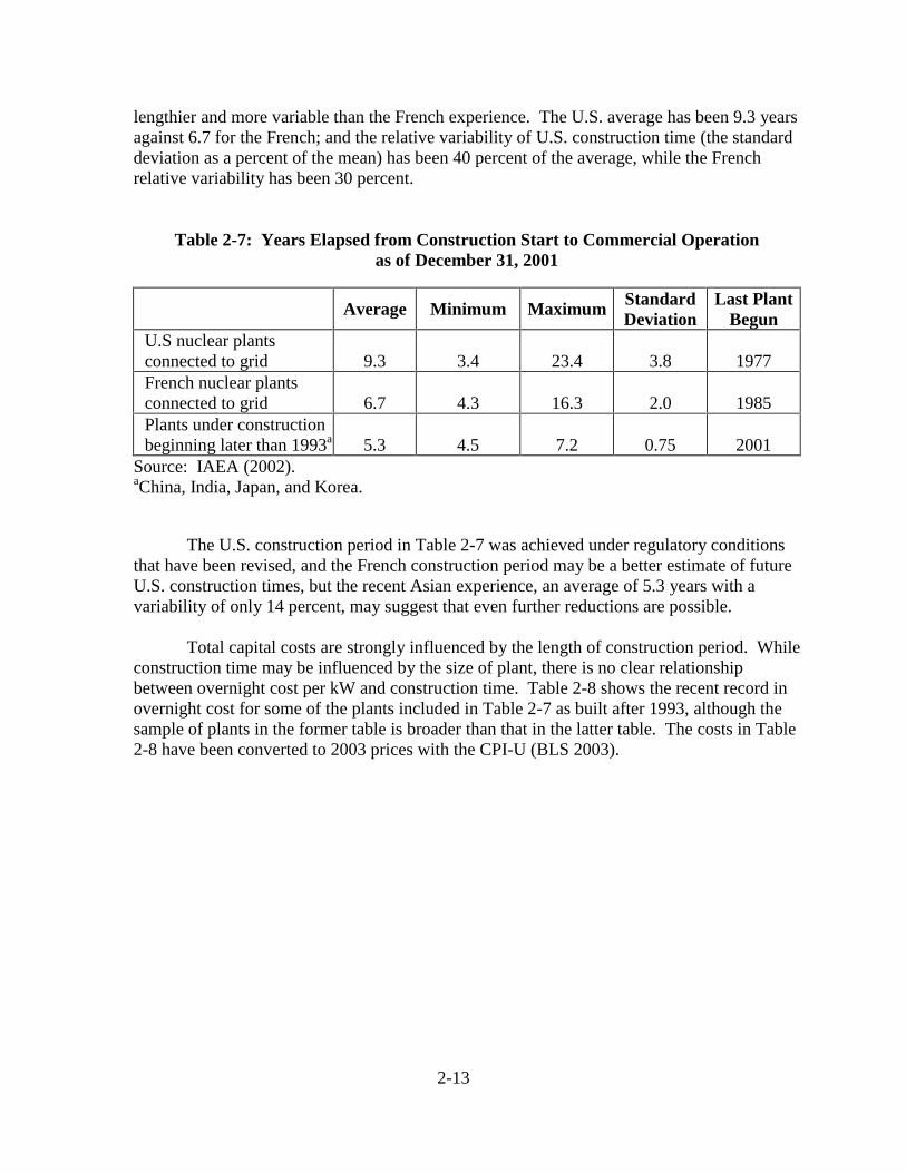
lengthier and more variable than the French experience. The U.S. average has been 9.3 yearsagainst 6.7 for the French; and the relative variability of U.S. construction time (the standarddeviation as a percent of the mean) has been 40 percent of the average, while the Frenchrelative variability has been 30 percent.

Table 2-7: Years Elapsed from Construction Start to Commercial Operationas of December 31, 2001

Average Minimum Maximum StandardDeviation

Last PlantBegun

U.S nuclear plantsconnected to grid 9.3 3.4 23.4 3.8 1977French nuclear plantsconnected to grid 6.7 4.3 16.3 2.0 1985Plants under constructionbeginning later than 1993a 5.3 4.5 7.2 0.75 2001

Source: IAEA (2002).aChina, India, Japan, and Korea.

The U.S. construction period in Table 2-7 was achieved under regulatory conditionsthat have been revised, and the French construction period may be a better estimate of futureU.S. construction times, but the recent Asian experience, an average of 5.3 years with avariability of only 14 percent, may suggest that even further reductions are possible.

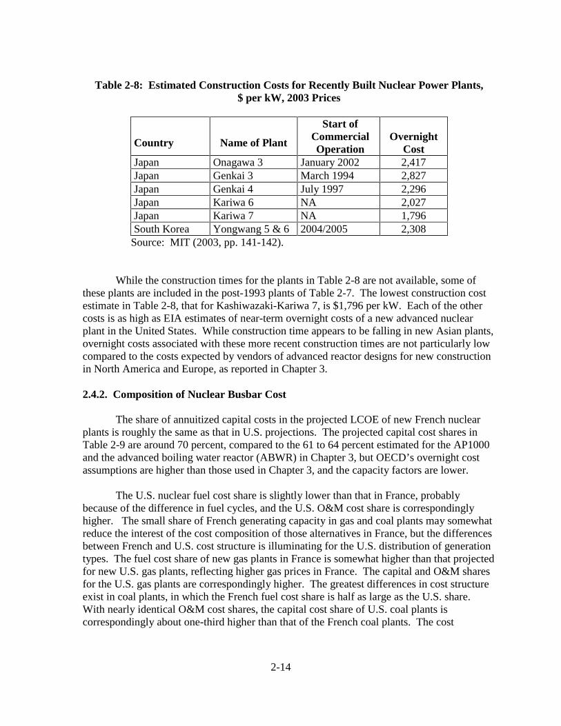
Total capital costs are strongly influenced by the length of construction period. Whileconstruction time may be influenced by the size of plant, there is no clear relationshipbetween overnight cost per kW and construction time. Table 2-8 shows the recent record inovernight cost for some of the plants included in Table 2-7 as built after 1993, although thesample of plants in the former table is broader than that in the latter table. The costs in Table2-8 have been converted to 2003 prices with the CPI-U (BLS 2003).

2-14

Table 2-8: Estimated Construction Costs for Recently Built Nuclear Power Plants,$ per kW, 2003 Prices

Country Name of Plant

Start ofCommercialOperation

OvernightCost

Japan Onagawa 3 January 2002 2,417 Japan Genkai 3 March 1994 2,827 Japan Genkai 4 July 1997 2,296 Japan Kariwa 6 NA 2,027 Japan Kariwa 7 NA 1,796 South Korea Yongwang 5 & 6 2004/2005 2,308

Source: MIT (2003, pp. 141-142).

While the construction times for the plants in Table 2-8 are not available, some ofthese plants are included in the post-1993 plants of Table 2-7. The lowest construction costestimate in Table 2-8, that for Kashiwazaki-Kariwa 7, is $1,796 per kW. Each of the othercosts is as high as EIA estimates of near-term overnight costs of a new advanced nuclearplant in the United States. While construction time appears to be falling in new Asian plants,overnight costs associated with these more recent construction times are not particularly lowcompared to the costs expected by vendors of advanced reactor designs for new constructionin North America and Europe, as reported in Chapter 3.

2.4.2. Composition of Nuclear Busbar Cost

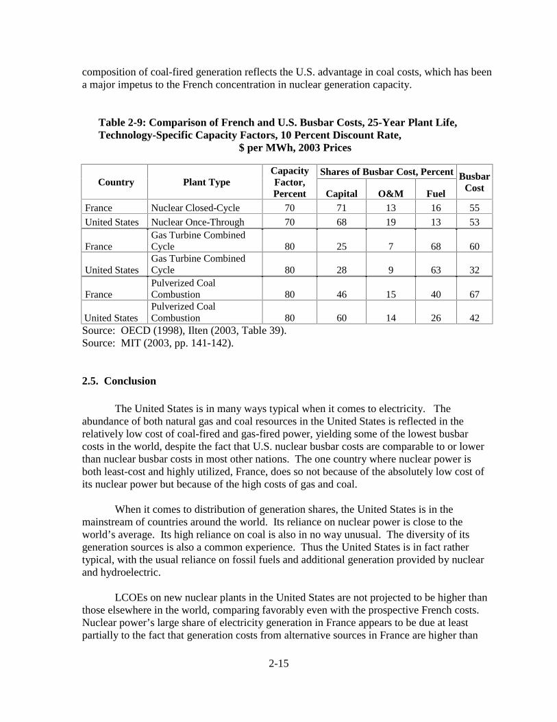
The share of annuitized capital costs in the projected LCOE of new French nuclearplants is roughly the same as that in U.S. projections. The projected capital cost shares inTable 2-9 are around 70 percent, compared to the 61 to 64 percent estimated for the AP1000and the advanced boiling water reactor (ABWR) in Chapter 3, but OECD’s overnight costassumptions are higher than those used in Chapter 3, and the capacity factors are lower.

The U.S. nuclear fuel cost share is slightly lower than that in France, probablybecause of the difference in fuel cycles, and the U.S. O&M cost share is correspondinglyhigher. The small share of French generating capacity in gas and coal plants may somewhatreduce the interest of the cost composition of those alternatives in France, but the differencesbetween French and U.S. cost structure is illuminating for the U.S. distribution of generationtypes. The fuel cost share of new gas plants in France is somewhat higher than that projectedfor new U.S. gas plants, reflecting higher gas prices in France. The capital and O&M sharesfor the U.S. gas plants are correspondingly higher. The greatest differences in cost structureexist in coal plants, in which the French fuel cost share is half as large as the U.S. share.With nearly identical O&M cost shares, the capital cost share of U.S. coal plants iscorrespondingly about one-third higher than that of the French coal plants. The cost

2-15

composition of coal-fired generation reflects the U.S. advantage in coal costs, which has beena major impetus to the French concentration in nuclear generation capacity.

Table 2-9: Comparison of French and U.S. Busbar Costs, 25-Year Plant Life,Technology-Specific Capacity Factors, 10 Percent Discount Rate,

$ per MWh, 2003 Prices

Shares of Busbar Cost, PercentCountry Plant Type

CapacityFactor,Percent Capital O&M Fuel

BusbarCost

France Nuclear Closed-Cycle 70 71 13 16 55

United States Nuclear Once-Through 70 68 19 13 53

FranceGas Turbine CombinedCycle 80 25 7 68 60

United StatesGas Turbine CombinedCycle 80 28 9 63 32

FrancePulverized CoalCombustion 80 46 15 40 67

United StatesPulverized CoalCombustion 80 60 14 26 42

Source: OECD (1998), Ilten (2003, Table 39).Source: MIT (2003, pp. 141-142).

2.5. Conclusion

The United States is in many ways typical when it comes to electricity. Theabundance of both natural gas and coal resources in the United States is reflected in therelatively low cost of coal-fired and gas-fired power, yielding some of the lowest busbarcosts in the world, despite the fact that U.S. nuclear busbar costs are comparable to or lowerthan nuclear busbar costs in most other nations. The one country where nuclear power isboth least-cost and highly utilized, France, does so not because of the absolutely low cost ofits nuclear power but because of the high costs of gas and coal.

When it comes to distribution of generation shares, the United States is in themainstream of countries around the world. Its reliance on nuclear power is close to theworld’s average. Its high reliance on coal is also in no way unusual. The diversity of itsgeneration sources is also a common experience. Thus the United States is in fact rathertypical, with the usual reliance on fossil fuels and additional generation provided by nuclearand hydroelectric.

LCOEs on new nuclear plants in the United States are not projected to be higher thanthose elsewhere in the world, comparing favorably even with the prospective French costs.Nuclear power’s large share of electricity generation in France appears to be due at leastpartially to the fact that generation costs from alternative sources in France are higher than

2-16

for nuclear power. Total capital cost shares of LCOEs for new nuclear plants projected in theUnited States and France are similar.

Historically, France has experienced shorter and less variable construction times forits nuclear plants than has the United States. Meanwhile, nuclear plants built since 1993,mostly in Asia, have been built in shorter times, and with lesser variability, than even theFrench experience, offering some basis for optimism regarding future nuclear construction inthe United States. However, the overnight costs of a sample of these recently built plantsremain high.

2.6. Appendix: LCOE Methodology

This appendix reports the formulations used in the calculations of the internationalLCOE comparison and discusses the cost and performance data used. The structure of thismodel is essentially the same as the pre-tax LCOE model of Chapter 1. Some minorspecification differences, which are implemented in the model of this chapter toaccommodate the structure of OECD data, are noted below.

2.6.1. Levelized Cost Formula

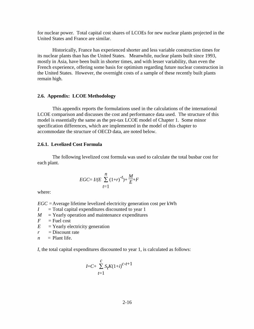
The following levelized cost formula was used to calculate the total busbar cost foreach plant.

EGC= I/(E ∑t=1

n (1+r)-t)+

ME+F

where:

EGC =Average lifetime levelized electricity generation cost per kWhI = Total capital expenditures discounted to year 1M = Yearly operation and maintenance expendituresF = Fuel costE = Yearly electricity generationr = Discount raten = Plant life.

I, the total capital expenditures discounted to year 1, is calculated as follows:

I=C+ ∑t=1

c StK(1+i)c-t+1

2-17

where:

I = Total capital expenditures discounted to year 1C = Contingency costsK = Overnight capital cost (excluding contingency costs)St = Percentage of overnight capital costs incurred in the tth year of construction

c = Length of construction period.

K, overnight capital cost (less contingency costs), is the dollar amount that would bepaid out if all capital expenses occurred simultaneously; no interest payments are included.OECD (1998) reports contingency costs separately from overnight costs, although the U.S.definition of overnight cost includes contingency costs and owner’s costs, as described ingreater detail in Chapter 3. This data reporting difference is responsible for the separateaccounting of contingency costs in the equation for capital costs above, which treatscontingencies as being expended in the final year of construction. E, yearly electricitygeneration is simply total nameplate capacity times capacity factor. F, the fuel cost, and M,the yearly operation and maintenance expenditures, were taken directly from each of the datasources.

All costs are reported in June 2003 U.S. mills per kWh. Costs from each data sourcewere first converted to dollars with the Federal Reserve exchange rates (Federal ReserveBoard 2001) if necessary, and then converted to June 2003 mills using the CPI-U (BLS2003).

2.6.2. Relationship to OECD Cost Formula

A significant portion of the cost data used in this study was drawn from OECD(1998). Thus it may be helpful to see the relationship between the cost formula used here andthe formula used in that study.

The OECD formula is a standard levelized cost formula, looking at the ratio betweenthe total sum of discounted costs and the total sum of discounted generation:

EGC= (∑t

[(It+Mt+Ft)(1+r)-t])/G

G= ∑t

[Et(1+r)-t]

where:

EGC= Average lifetime levelized electricity generation cost per kWh

It = Capital expenditures in the year t

2-18

Mt = Operation and maintenance expenditures in the year t

Ft = Fuel expenditures in the year t

Et = Electricity generation in the year t

r = Discount rate.

The summation is carried out over the entire life of the plant, beginning with planningand construction and lasting until decommissioning is over.

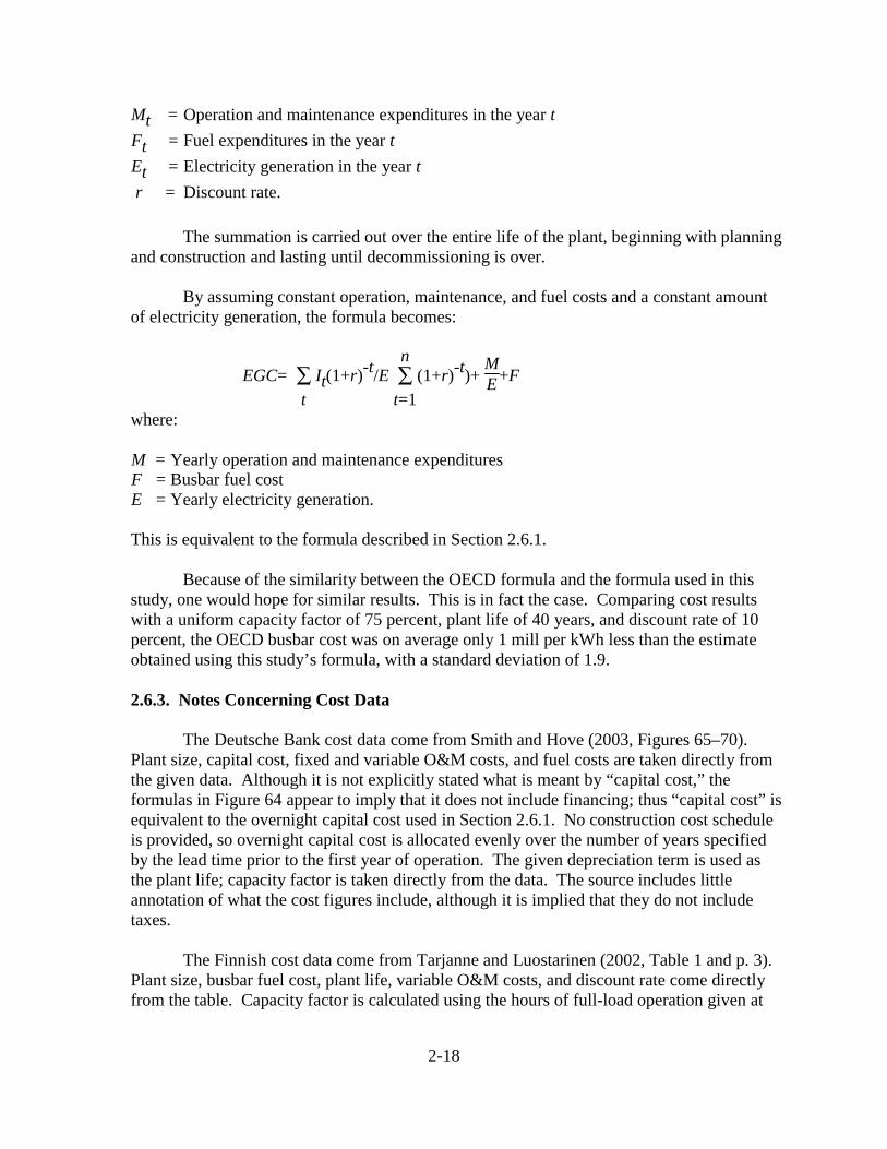
By assuming constant operation, maintenance, and fuel costs and a constant amountof electricity generation, the formula becomes:

EGC= ∑t

It(1+r)-t/E ∑t=1

n (1+r)-t)+

ME+F

where:

M = Yearly operation and maintenance expendituresF = Busbar fuel costE = Yearly electricity generation.

This is equivalent to the formula described in Section 2.6.1.

Because of the similarity between the OECD formula and the formula used in thisstudy, one would hope for similar results. This is in fact the case. Comparing cost resultswith a uniform capacity factor of 75 percent, plant life of 40 years, and discount rate of 10percent, the OECD busbar cost was on average only 1 mill per kWh less than the estimateobtained using this study’s formula, with a standard deviation of 1.9.

2.6.3. Notes Concerning Cost Data

The Deutsche Bank cost data come from Smith and Hove (2003, Figures 65–70).Plant size, capital cost, fixed and variable O&M costs, and fuel costs are taken directly fromthe given data. Although it is not explicitly stated what is meant by “capital cost,” theformulas in Figure 64 appear to imply that it does not include financing; thus “capital cost” isequivalent to the overnight capital cost used in Section 2.6.1. No construction cost scheduleis provided, so overnight capital cost is allocated evenly over the number of years specifiedby the lead time prior to the first year of operation. The given depreciation term is used asthe plant life; capacity factor is taken directly from the data. The source includes littleannotation of what the cost figures include, although it is implied that they do not includetaxes.

The Finnish cost data come from Tarjanne and Luostarinen (2002, Table 1 and p. 3).Plant size, busbar fuel cost, plant life, variable O&M costs, and discount rate come directlyfrom the table. Capacity factor is calculated using the hours of full-load operation given at

2-19

Tarjanne and Luostarinen (2002, p. 5). Fixed O&M costs are calculated by multiplying thegiven cost percentage by the given investment cost. However, these investment costs are notused as the overnight capital costs. No construction cost schedules are given, so OECDschedules are used. Finland’s OECD schedules are used for coal, gas and nuclear. Overnightcapital costs are calculated by solving for the cost figure yielding the total investmentdiscounted to year 1, given the construction schedules and a 5 percent discount rate. That is,the following equation is solved for K:

I= ∑t=1

c StK(1.05)c-t+1

where:

I = Total capital expenditures discounted to year 1K = Overnight capital costSt = Percentage of overnight capital costs incurred in the tth year of construction

c = Length of construction period.

No mention is made of contingency costs, so they are omitted. Costs include initialfuel loading for the nuclear plant, but do not include value-added-tax.

The OECD cost data come from OECD (1998, Tables 1–17). Plant size, contingencycost, overnight capital cost, construction schedules, total O&M costs, capacity factor, anddiscount rate are taken directly from the given data. No construction schedules are providedfor the fuel oil plant in Turkey, so all costs occur in the year previous to operation. Factorscovered in the costs vary by country and are detailed in Annex 7 of that report. In general,taxes are not included in the costs.

2-20

References

Bouchard, Jacques. (2003) Letter to Philippe Finck, Associate Director, Argonne NationalLaboratory. Director, Commissariat � l’énergie atomique. Paris, September 17.

Bureau of Labor Statistics (BLS). (2003) Consumer Price Index. All Urban Consumers -(CPI-U). U.S. City Average. Retrieved August 7, 2003 from the World Wide Web:ftp://ftp.bls.gov/pub/special.requests/cpi/cpiai.txt.

Charpin, Jean-Michel, Benjamin Dessus, and René Pellat. (2000). Economic Forecast Studyof the Nuclear Power Option. Report to the Prime Minister. Paris: Commissariat Generaldu Plan, July.

Drennan, Thomas E., Arnold B. Baker, and William Kamery. (2002) Electricity GenerationCost Simulation Model (GenSim). SAND2002-3376. Albuquerque, N.M.: Sandia NationalLaboratories, November.

Energy Information Administration (EIA). (2002) The Electricity Market Module of theNational Energy Modeling System. Washington, D.C.: Energy Information Administration.

Federal Reserve Board. (2001) Foreign Exchange Rates. November 30, 2001. RetrievedAugust 7, 2003 from the World Wide Web:http://www.federalreserve.gov/releases/G5/20011203.

Feretic, Danilo, and Tomsic Zeljko. (2003) “Probabilistic Analysis of Electrical EnergyCosts Comparing: Production Costs for Gas, Coal and Nuclear Power Plants,” forthcomingin Energy Policy, available online August 8.

Ilten, Nathan. (2003) “International Comparisons of Electricity Generation by Types &Costs.” Mimeo. Chicago: University of Chicago, August.

International Association of Atomic Energy (IAEA). (2002) Country Nuclear PowerProfiles. Retrieved July 5, 2003 from the World Wide Web:http://www-pub.iaea.org/MTCD/publications/PDF/cnpp2002/index.htm.

International Energy Agency (IEA). (2000) Electricity Information 2000. Paris: OECD.

Lescouer, Bruno, and Philippe Penz. (1999) La problématique du financement duinvestissements électronucléaires,” Revue de économie financi�re 51: 167-182.

Massachusetts Institute of Technology (MIT). (2003) The Future of Nuclear Power: AnInterdisciplinary MIT Study. Cambridge, Mass.: Massachusetts Institute of Technology,July.

2-21

Organization for Economic Co-operation and Development (OECD). (1998) ProjectedCosts of Generating Electricity. Update 1998. Paris: OECD.

Smith, R., and A. Hove. (2003) “The Old Reliables: Coal, Nuclear and Gas in 2003.”Report. New York: Deutsche Bank AG.

Tarjanne, Risto, and Kari Luostarinen. (2002) Economics of Nuclear Power in Finland.Lappeenranta, Finland: Lappeenranta University of Technology, June.

2-22

3-1

Chapter 3. CAPITAL COSTS

Summary

Capital costs are the single most important component of the costs of providingnuclear power, as is illustrated by figures from one of the major technologies considered indetail in this chapter. For the Advanced Boiling Water Reactor (ABWR), already built inAsia, the overnight capital costs, or undiscounted capital outlays, account for over one-thirdof LCOE, and the interest costs on the overnight costs account for another quarter of theLCOE.

Overnight Costs

Overnight cost estimates from different sources have ranged from less than $1,000per kW to as much as $2,300 per kW. This chapter examines reasons for differences inestimates, with the aim of reaching a smaller range.

The first major component of overnight costs consists of engineer-procure-construct,or EPC, costs, amounting to around 85 percent of total overnight costs paid. EPC costs are inturn separated into direct and indirect costs. The direct costs are for physical plant equipmentand the labor and materials to assemble them, while the indirect costs involve supervisoryengineering and support labor costs, with some materials. Direct costs account for roughly70 percent of EPC costs. About 60 percent of EPC costs are for factory equipment, 25percent for labor, and 15 percent for materials. About 50 percent of EPC costs are for reactorplant and turbine equipment. These figures include equipment, labor, and materials costs ofinstalling them. R&D targeted at these components could have a substantial impact onovernight cost.

Overnight costs include three additional categories of costs, one for contingencies,one for the owner’s costs of infrastructure and training incurred to get the plant runningsafely when it is built, and one for first-of-a-kind engineering, or FOAKE, costs.

Contingencies and owner’s costs can add 15 to 20 percent to overnight costs. Beforea reactor of a particular design has been built, several hundred million dollars must beexpended to complete its engineering design specifications. These are FOAKE costs. Theyare incurred only once for any type of reactor—although building a reactor of a particulardesign in one country may not transfer all the preliminary engineering necessary to satisfysafety regulations in another country, so some FOAKE costs may still be incurred for the firstconstruction in any given country. Nonetheless, when a U.S. firm builds a new designoverseas, much of the engineering experience may be transferable to the home country,making it possible for routine engineering and home office services to cover those remainingcosts.

FOAKE costs are a fixed cost of a particular reactor design. How a vendor allocatesFOAKE costs across all the reactors it sells can affect the overnight cost of early reactors

3-2

considerably. A vendor may be concerned about ability to sell multiple reactors and want torecover all FOAKE costs on its first plant. That could raise the overnight cost of the firstplant by 35 percent.

FOAKE costs are to be distinguished from nth-of-a-kind capital costs, which are theconsequence of learning by doing beyond the first-of-a kind construction and are consideredin the next chapter.

Interest Costs

Meanwhile, interest costs accrued during construction greatly affect total capitalcosts. By the time a new plant comes on line, total capital cost that electricity sales mustcover to repay investors can be 25 to 80 percent greater than the overnight costs, dependingon the interest rates and the length of the construction period.

How to deal with the sensitivity of nuclear capital costs to interest rates, as dependenton risk premium and length of construction periods, is dealt with in Chapter 5.

Overnight Cost Sensitivity Scenarios for the Present Study

In addition, much is accomplished in narrowing the range of uncertainty in capitalcosts by realistic specifications of reactors likely to be used and by attention to FOAKE costassumptions. The ABWR, the CANDU ACR-700, the AP1000, and Framatome’s SWR1000 appear to be reasonable candidates for deployment in the United States within thecoming decade.

The ABWR is a mature design, having been built recently in Japan by a U.S. firmteaming with a Japanese firm, so its FOAKE costs may be considered already paid. Anovernight cost of $1,246 per kW is justifiable for it. The CANDU ACR-700 has had units ofa closely related model, the CANDU 6, built recently in China and Romania. Constructiontimes have been short, and vendor estimates of overnight costs are quite low, around $1,000per kW, although EIA estimates $1,100 to $1,200 per kW for a third-of-a-kind twin unit. Itscost characteristics would appear to overlap those of the ABWR, despite their sizedifferences (1,350 MW versus 753 MW), so the first reactor design chosen for analysis maybe considered as representing either the ABWR or the ACR-700.

The AP1000 is closely related in design to the already certified AP600, but neitherdesign has been built yet, so its FOAKE costs remain to be paid. Assuming its entireFOAKE costs are paid on the first plant, $1,500 per kW is a justifiable overnight cost. TheSWR 1000 is based on design features proven in the European market. In meetings with theU.S. Nuclear Regulatory Commission (NRC), Framatome has expressed its intent to applyfor certification to enter the U.S. market with the design. Framatome’s European PressurizedWater Reactor (EPR) has been selected for construction in Finland. Estimates for the EPR inFinland suggest an overnight cost of $1,800 per kW for that reactor design, which wouldroughly parallel those of the SWR 1000.

3-3

Consideration of the foregoing reactor types contributes to the choice of $1,200,$1,500, and $1,800 per kW overnight costs in the sensitivity scenarios used in the economicviability analysis in Chapters 5 and 9. The range is consistent with allowance for uncertaintyin the cost estimates in view of the scope for variation in overnight costs due to the otherfactors reviewed in this chapter.

3-4

Outline

3.1. Introduction

3.2. Overnight Costs

3.2.1. Why Overnight Costs Differ3.2.2. Categories of Overnight Capital Costs3.2.3. FOAKE Costs and Capital Cost Estimates3.2.4. Learning by Doing3.2.5. Other Sources of Overnight Capital Cost Reduction3.2.6. Near-Term Reactor Designs3.2.7. Cost Implications of Opportunities for Siting New Nuclear Plants

3.3. The Shares of Overnight Capital Costs and Interest Costs in LCOE

3.4. Reactor Designs and Capital Cost Scenarios for Economic Analysis

3.5. Uncertainty in Overnight Cost Estimates

References

3-5

3.1. Introduction

Capital costs are especially important to the competitiveness of nuclear power, sincethey account for a major share of the levelized cost of electricity (LCOE). The literature onnuclear power plant costs reports a wide array of capital costs. In analyzing why theestimates differ, Section 3.2 of this chapter deals with the overnight cost component ofcapital costs. Section 3.3 deals with the interest component. Section 3.4 uses the results ofthe chapter to narrow the range of capital costs to be used in the economic analysis of thepresent study, proposing to limit the analysis to three near-term reactors as the most realisticpossibility and to allow for remaining uncertainty based on analysis of the individualcomponents of capital costs.

3.2. Overnight Costs

3.2.1. Why Overnight Costs Differ

Estimates of overnight capital costs of nuclear plants have ranged from as high as$2,300 per kW and to as low as $1,100 per kW. The reasons for the differences are diverse.At the simplest explanation, the numbers refer to different reactor technologies. Estimatesfor the same technology can differ as well, however. At different times, the cost estimatesfor reactor components may differ, and of course, different price levels prevail at differentdates, so cost estimates produced at different dates should be adjusted for price-leveldifferences for comparability.

A further important source of cost difference, for identical as well as differenttechnologies is the allowance for contingencies. Reactor cost quotes are firm-fixed-priceoffers (even if they may be subject to negotiation between vendor and buyer), and vendorsinclude allowances for construction costing more than their most optimistic estimate. Thesecosts are included in an account explicitly referred to as contingencies and are charged to thebuyer whether the contingent events occur or not. Depending on how much of thecontingency costs actually get expended—which can be more or less than 100 percent—avendor’s profits on a project will vary.

Cost numbers sometimes refer to expected costs in different countries, and marketcosts of inputs may differ across countries, for which purchasing power parity adjustmentsare imperfect. When considering cost numbers of technologies of firms from differentcountries, the possibility should be considered that governments are offering subventions forsome proportion of costs.

Some cost numbers refer to actual construction costs where others are expected costsof plants not yet built. For reactors that have not been built, some estimates may includeFOAKE costs while others may exclude them. Frequently costs are expressed in terms ofnth-of-a-kind and possibly combined with twin plant assumptions. The nth-of-a-kind cost hasreduced the first-plant cost by some presumed learning efficiency

3-6

in construction, often assumed to be 5 percent for each doubling of the number of plants builtof the specified type. With twin plants, greater cost reductions are expected. If two reactorsare built at the same site at the same time, some experience suggests that both can be built for5 to 7 percent less than if they were built separately, either at different sites at the same timeor at the same site at different times. The cost reduction derives from the ability to schedulework crews and construction equipment more expeditiously, with less down-time, as well aseconomies in procurement and related support costs. This phenomenon will be consideredmore fully in the next chapter.

When a publication gives an overnight capital cost number for a nuclear power plant,some of these qualifications may appear in footnotes, but most often, some will be omitted.

3.2.2. Categories of Overnight Capital Costs

Capital costs are customarily separated into three principal types of expenditurewhich are allocated across ten or eleven accounts. Table 3-1 identifies the accounts andreports a typical structure of capital cost accounts for a nuclear power plant for a boilingwater reactor of mature design. Table 3-2 disaggregates the expenditures by account for themature boiling water reactor into their three principal components, equipment, labor, andmaterials, reporting the structure of costs in more detail. The cost structure of Table 3-2 issimilar to the cost structures reported for a variety of reactors in Nuclear Energy Agency(NEA), 2000, Table 5, p. 29.

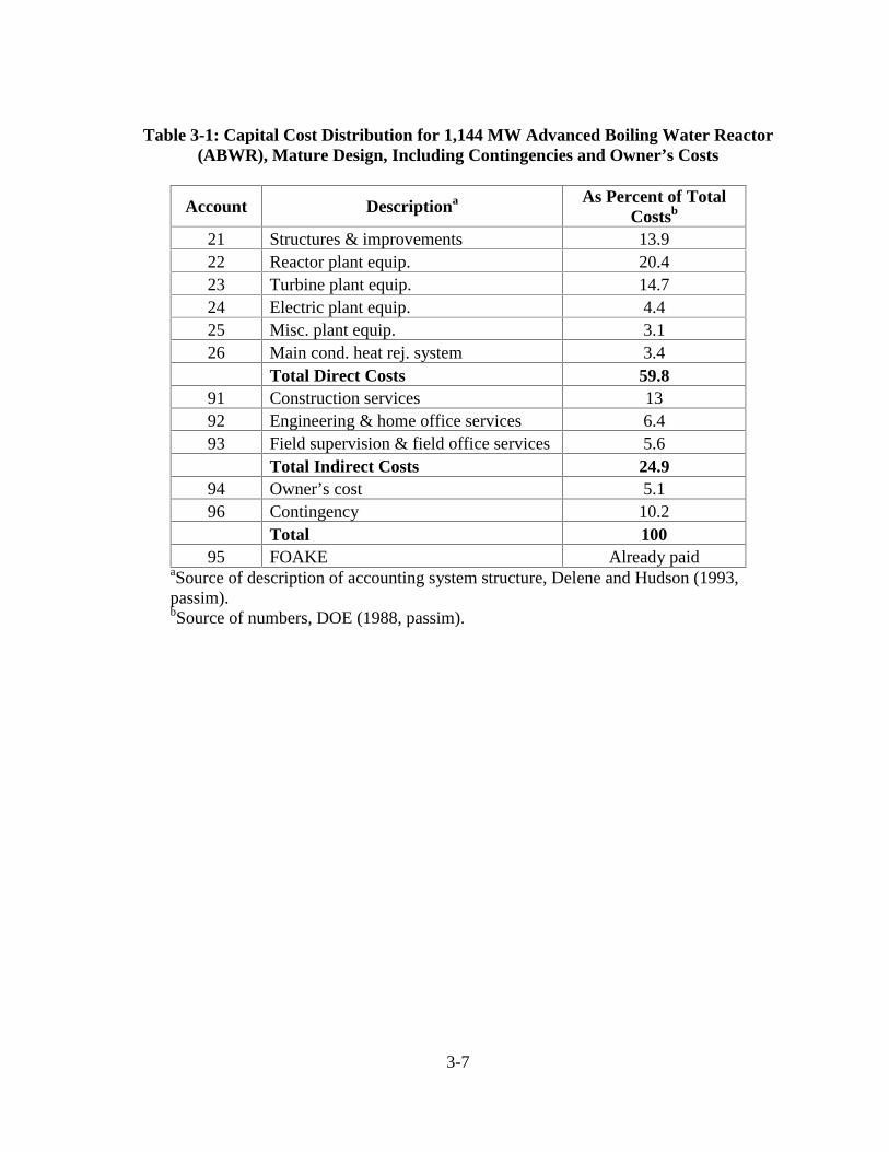
3-7

Table 3-1: Capital Cost Distribution for 1,144 MW Advanced Boiling Water Reactor(ABWR), Mature Design, Including Contingencies and Owner’s Costs

Account Descriptiona As Percent of TotalCostsb

21 Structures & improvements 13.922 Reactor plant equip. 20.423 Turbine plant equip. 14.724 Electric plant equip. 4.425 Misc. plant equip. 3.126 Main cond. heat rej. system 3.4 Total Direct Costs 59.8

91 Construction services 1392 Engineering & home office services 6.493 Field supervision & field office services 5.6 Total Indirect Costs 24.9

94 Owner’s cost 5.196 Contingency 10.2 Total 100

95 FOAKE Already paidaSource of description of accounting system structure, Delene and Hudson (1993,passim).bSource of numbers, DOE (1988, passim).

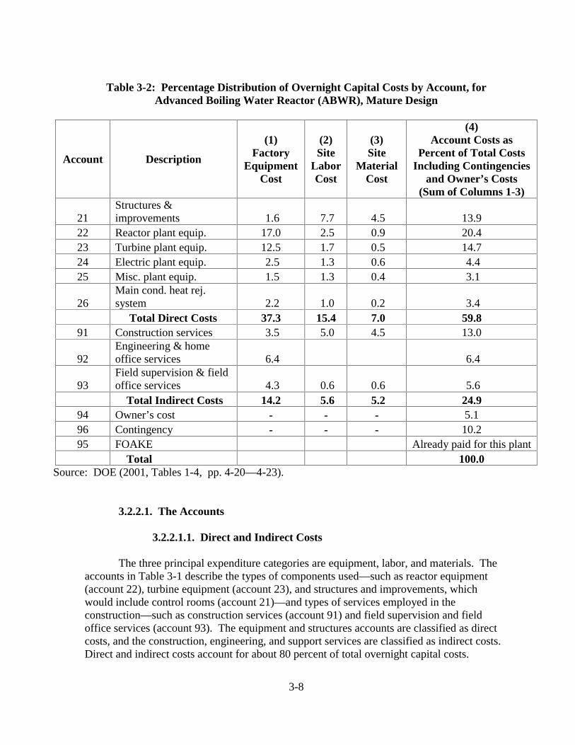
3-8

Table 3-2: Percentage Distribution of Overnight Capital Costs by Account, forAdvanced Boiling Water Reactor (ABWR), Mature Design

Account Description

(1)Factory

EquipmentCost

(2)Site

LaborCost

(3)Site

MaterialCost

(4)Account Costs as

Percent of Total CostsIncluding Contingencies

and Owner’s Costs(Sum of Columns 1-3)

21Structures &improvements 1.6 7.7 4.5 13.9

22 Reactor plant equip. 17.0 2.5 0.9 20.423 Turbine plant equip. 12.5 1.7 0.5 14.724 Electric plant equip. 2.5 1.3 0.6 4.425 Misc. plant equip. 1.5 1.3 0.4 3.1

26Main cond. heat rej.system 2.2 1.0 0.2 3.4 Total Direct Costs 37.3 15.4 7.0 59.8

91 Construction services 3.5 5.0 4.5 13.0

92Engineering & homeoffice services 6.4 6.4

93Field supervision & fieldoffice services 4.3 0.6 0.6 5.6 Total Indirect Costs 14.2 5.6 5.2 24.9

94 Owner’s cost - - - 5.196 Contingency - - - 10.295 FOAKE Already paid for this plant

Total 100.0 Source: DOE (2001, Tables 1-4, pp. 4-20—4-23).

3.2.2.1. The Accounts

3.2.2.1.1. Direct and Indirect Costs

The three principal expenditure categories are equipment, labor, and materials. Theaccounts in Table 3-1 describe the types of components used—such as reactor equipment(account 22), turbine equipment (account 23), and structures and improvements, whichwould include control rooms (account 21)—and types of services employed in theconstruction—such as construction services (account 91) and field supervision and fieldoffice services (account 93). The equipment and structures accounts are classified as directcosts, and the construction, engineering, and support services are classified as indirect costs.Direct and indirect costs account for about 80 percent of total overnight capital costs.

3-9

3.2.2.1.2. Contingencies

To these direct and indirect costs, vendors add a percentage referred to ascontingencies (account 96). They will need to justify these contingency costs to a buyer, andthey may be negotiated. Sometimes a government will agree to pay contingency costs.These may range from 9 to 12 percent of total direct and indirect costs, or be as low as zero.

3.2.2.1.3. Owner’s Costs

Another category of costs, owner’s cost (account 94), is paid directly by the buyer.These are costs of testing systems within the plant, training a staff (which may take severalyears while the plant is being built), various inspections, etc. These range from 5 to 10percent of direct and indirect costs.

3.2.2.1.4. FOAKE Costs

Accounting practices for nuclear power plant costs have evolved in recent years, andthe identification of the costs of working out the initial engineering design of a new type ofreactor as a distinct type of cost is an important product of that development. When a newtype of reactor is developed, taking that design from relatively simple conceptual stages todetailed engineering specifications that will make all the necessary components cometogether successfully is a massive undertaking. These costs can range from $300 million to$600 million, adding as much as 30 percent to the cost of a first reactor. However, oncethese design efforts are completed, they never have to be repeated for this reactor design.Further engineering design work will have to be undertaken to place this type of reactor intoa particular site, with its particular geographical and geological setting, but those engineeringcosts are contained in account 92, engineering and home office services.

FOAKE costs are specific to each reactor design. For example, two new reactordesigns, say the AP1000 and the ABWR would have completely separate FOAKE costs.However, if one of these designs were to be built in, say, China, a considerable portion, butnot all, of the FOAKE costs of building it in the United States would be covered by thedesign work for the Chinese installation. This reduction, if not elimination, of FOAKE costsby building a new reactor in any particular country, is motivation for more aggressive initialpricing in overseas markets.

How a vendor accounts for these FOAKE costs can make a substantial difference inthe capital cost estimate. The effects of accounting for FOAKE costs are discussed further inSection 3.4 below.

3.2.2.2. The Account Structure of Capital Costs

Table 3-1 shows the largest component of overnight capital costs to be the reactorequipment. This account amounts to 20 percent of total costs, including owner’s costs and

3-10

contingencies. Following the reactor equipment in cost share is the turbine equipment,followed closely in turn by structures and improvements. The turbine equipment accountsfor 15 percent of the total. Structures and equipment account for 14 percent of the costs.Electric plant equipment, miscellaneous plant equipment, and main conditioning heatrejection systems each account for 3 to 4 percent of costs. Total direct costs amount to60 percent of total costs.

Indirect costs are comprised of construction services, engineering and home officeservices, and field supervision and field office services. Construction services, which are theactual building and assembly of the components into a functioning plant, are the largestindirect cost component. Engineering and home office services include engineering designcosts required to adapt a fully known reactor design into a particular site, as well asprocurement and other administrative services required to support construction. It includesno FOAKE costs, as this may be considered a mature design. Field supervision and fieldoffice services involve the supervision of construction, including on-site engineering andadministrative support activities. Indirect costs account for 25 percent of the costs.

Owner’s cost accounts for an additional 5 percent of the costs. Contingencies are 10percent of total costs.

3.2.2.3. The Composition of the Capital Cost Accounts

Table 3-2 disaggregates the overnight cost accounts of the mature design ABWR intoequipment, labor, and materials cost components. Equipment costs dominate total costsaccounting for 52 percent of total costs. Labor accounts for 21 percent of costs, andmaterials for the remaining 12 percent. In column 1, equipment costs for the reactor (account22) and the turbine equipment (account 23) account for fully 30 percent of total costs. Themost significant labor costs are in structures and improvements (account 21), at nearly8 percent of total costs.

3.2.2.4. Cost Uncertainties

Excluding contingencies, labor costs may be the greatest source of cost uncertainty.Strikes or other sources of labor productivity variance can operate on a quarter of total directand indirect costs. A 25 percent overrun in labor costs would add 5 percent to total costs.

Once a particular reactor design has been built, and its equipment componentssupplied, the factory equipment cost shares should be quite predictable, but the equipmentcosts of reactor and turbine components for a new design may well vary 20 percent aroundthe base cost shares shown in Table 3-2 for this mature reactor design. If factory equipmentcosts in these two accounts (22 and 23) both were 20 percent higher than the estimates forwhich Table 3-2 presents cost shares, total costs would increase by 7 percent.

3-11

3.2.2.5. Possible Effect of Strategic Considerations

Several reasons exist why overnight cost estimates are not entirely hard engineeringestimates. For example, if a vendor finds some indirect value to building a plant (especially afirst plant or a first plant in a particular market), it may depress its contingency costcomponent, possibly eliminating it altogether, in order to obtain the sale. If some of thecontingent events do occur, the vendor may well have to take the associated costs out of itsprofits. In some instances in which national governments have particularly close associationswith their countries’ nuclear vendors, the governments may agree to help with contingencies,although these actions may be limited by international trade agreements. A vendor might beable to get a variance agreement with the buyer to reimburse additional costs, particularly butnot exclusively, in force majeure cases.

Cost estimates may be influenced by marketing goals. When comparing costestimates for different types of reactors, produced by different vendors, it is even possiblethat one cost estimate is a strategic marketing reaction to another cost estimate. Account 96,contingencies, is available to assist a vendor in strategic marketing goals, with or withoutgovernment subventions.

3.2.3. FOAKE Costs and Capital Cost Estimates

Section 3.2.1 introduced FOAKE costs, and noted that they can add 30 percent tototal overnight costs. FOAKE costs are a fixed cost of a reactor design. If a lengthyproduction run reasonably could be assured, comparable to, say, a new model of automobile,the costs can be amortized over the anticipated future production and have little effect on theunit price. Conditions have not proven as simple for nuclear reactors.

How a vendor chooses to account for FOAKE costs may affect price and even itsability to sell a reactor. The preferred method, of course, is to have the vendor’s governmentpay for these costs, but the practicality of that alternative depends on the priorities ofdifferent countries’ governments. An agreement with a utility or consortium of utilities forthe purchase of multiple reactors, possibly eight or ten, spread out over a relatively short timeperiod, would be an alternative that would permit the spread of these fixed costs overmultiple units. However, any utility or consortium accepting such a cost agreement wouldeffectively subsidize subsequent buyers of this design, which reduces the likelihood of suchan arrangement being reached in practice.

No a priori solution to this problem is apparent. Vendors may deal with the pricingproblem by either (1) quoting nth-of-a-kind costs, which exclude FOAKE costs and includecost reductions due to learning over the construction of the first n-1 reactors or (2) quotingcapital cost for a first plant in $ per kW terms and placing the FOAKE cost alongside as acover charge.

3-12

3.2.4. Learning by Doing

The nth-of-a-kind costs were introduced above, in Section 3.2.2, as including the cost-reducing effects of learning from previous construction and manufacturing experience. Thiscost reduction excludes the FOAKE cost that might be associated with the first reactor built.The cost reductions derived from learning by doing and the elimination of sunk FOAKEcosts are quite different conceptually, as this section emphasizes. The magnitude of learningeffects is expressed as the percent reduction in cost associated with a doubling of the numberof plants built. For example, an x percent learning rate means that the second plant will costx percent less than the first plant, that the fourth plant will cost x percent less than the secondplant, the eighth plant will cost x percent less than the fourth plant, and so on. The costreductions decrease with continued construction although the learning rate is constant. Theempirical evidence on the magnitudes of these effects is presented in Chapter 4.

Three principal sources of learning in nuclear construction may be distinguished. Thefirst source of learning by doing cost reductions is in the factory, with vendors and theirequipment. Engineers and skilled workers learn ways to produce components in less timeand possibly fewer wasted materials. The second source of learning by doing in nuclearpower plant construction is on-site replication—construction by the same contractor at thesame site over a short time span. Engineering staffs and construction crews can be kepttogether so as to retain their learning and teamwork from previous experience. The thirdsource of learning by doing is between-sites replication, in which the cost reductions derivefrom plant standardization even though engineering staffs and construction crews maychange.

Each of these sources of learning is largely independent of the other sources, butsimilar factors can affect each. The short time span of multiple construction jobs required forthe cost-reduction benefits of on-site replication applies to a considerable extent to thefactory learning by vendors. If orders arrive more or less continuously, factory staffs aremaintained, but if lengthy delays occur between orders, staffs may be let go and have to bereassembled and retrained subsequently, reducing the learning benefits of more continuousproduction. Similarly with the between-sites replication, although more of the plantstandardization benefits may survive lengthy intervals between orders. Under favorablecircumstances, such as steady building activity concentrated at single sites, learning effectswill be greater than under less favorable circumstances.

3.2.5. Other Sources of Overnight Capital Cost Reduction

Another principal source of cost reduction that can be affected by constructionpatterns is the multi-unit station effect noted in Section 3.3. Scheduling economies, as wellas some fixed indirect costs such as purchasing and other administrative activities, haveproved to result in reductions in overnight costs if two or more reactors can be builtsimultaneously at the same power station. A review of international construction experiencesuggests that savings from multiple-unit construction have averaged around 15 percent of the

3-13

overnight cost of a single-unit construction (NEA 2000, pp. 12-13, 65-70). This effect isindependent of learning effects, which themselves may be enhanced by building multiplereactors at a single station, as reported in Chapter 4.

Significant cost reduction also may derive from standardization of plant design.Much of this cost saving is thought to lie in reduction of overnight costs by eliminatingduplication in FOAKE costs. Reductions in construction time from standardization alsoreduce interest costs (NEA 2000, pp. 12, 55-65). Again, these cost savings are distinct fromthe effect of standardization on learning by doing.

3.2.6. Near-Term Reactor Designs

Table 3-3 gives dollar figures underlying the percentages in Table 3-1.

Table 3-3: Capital Cost Estimates: Advanced Boiling Water Reactor (ABWR),Mature Design, in Millions of 2001 Dollars

Account Description ABWR21 Structures & improvements 19822 Reactor plant equip 290

23 Turbine plant equip 21024 Electric plant equip 6225 Misc. plant equip 4526 Main cond. ht rej. system 48

Total Direct Costs 85391 Construction services 18692 Engineering & home office services 9193 Field supervision & field office services 79

Total Indirect Costs 35694 Owner’s cost 7396 Contingency 145

Total 1,426Source: ABWR, DOE (2001, Tables 1-4) and consultation with internationaltechnical nuclear expert.

For comparison, a published Westinghouse estimate for total costs of an AP1000reactor, without FOAKE costs, is $1,100 to $1,200 per kW (Poulson 2002, p. 22). This figureis slightly below the $1,246 per kW for the ABWR in Table 3-3 (as implied by dividing thetotal cost in Table 3-3 by 106 to obtain dollars and 1,144, which is the capacity in megawattsof the ABWR). However, the AP1000 has not yet been built. Assigning a FOAKE cost of

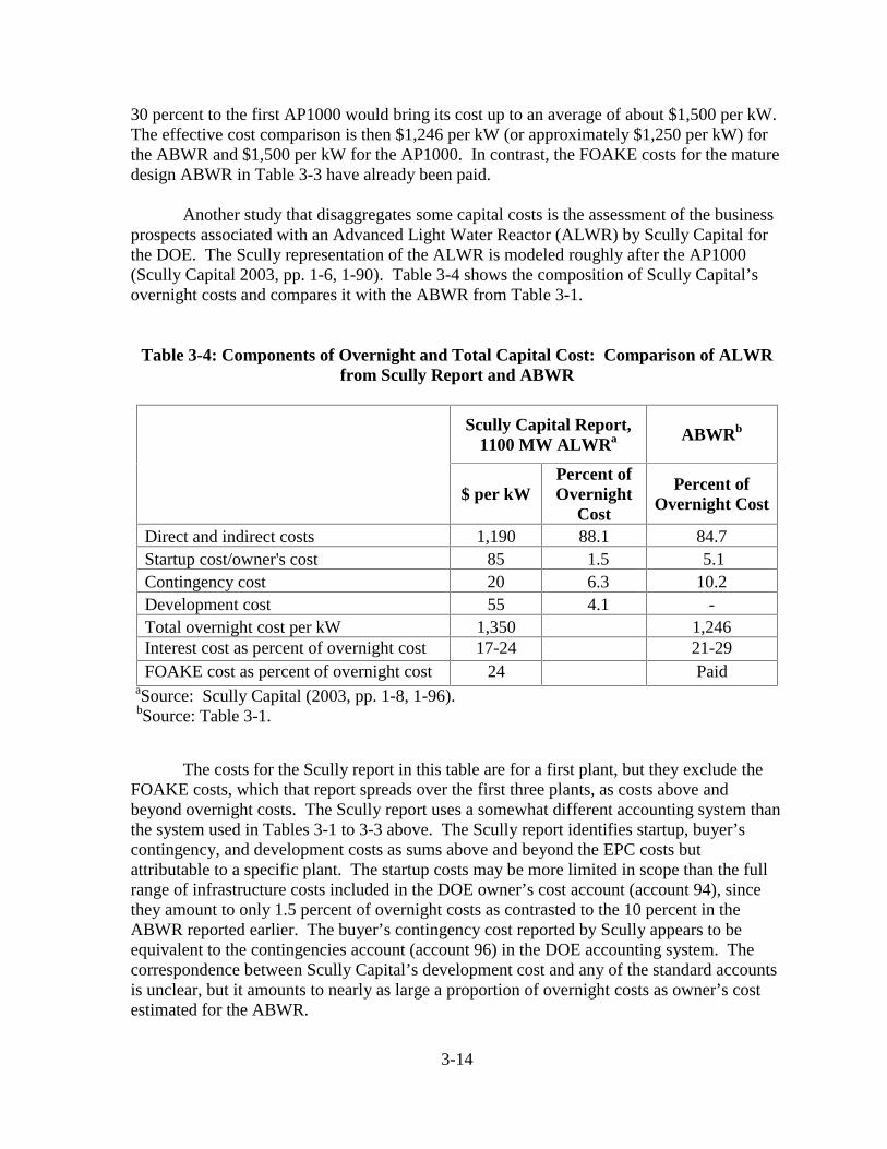
3-14

30 percent to the first AP1000 would bring its cost up to an average of about $1,500 per kW.The effective cost comparison is then $1,246 per kW (or approximately $1,250 per kW) forthe ABWR and $1,500 per kW for the AP1000. In contrast, the FOAKE costs for the maturedesign ABWR in Table 3-3 have already been paid.

Another study that disaggregates some capital costs is the assessment of the businessprospects associated with an Advanced Light Water Reactor (ALWR) by Scully Capital forthe DOE. The Scully representation of the ALWR is modeled roughly after the AP1000(Scully Capital 2003, pp. 1-6, 1-90). Table 3-4 shows the composition of Scully Capital’sovernight costs and compares it with the ABWR from Table 3-1.

Table 3-4: Components of Overnight and Total Capital Cost: Comparison of ALWRfrom Scully Report and ABWR

Scully Capital Report,1100 MW ALWRa ABWRb

$ per kWPercent ofOvernight

Cost

Percent ofOvernight Cost

Direct and indirect costs 1,190 88.1 84.7Startup cost/owner's cost 85 1.5 5.1Contingency cost 20 6.3 10.2Development cost 55 4.1 -Total overnight cost per kW 1,350 1,246Interest cost as percent of overnight cost 17-24 21-29FOAKE cost as percent of overnight cost 24 Paid

aSource: Scully Capital (2003, pp. 1-8, 1-96). bSource: Table 3-1.

The costs for the Scully report in this table are for a first plant, but they exclude theFOAKE costs, which that report spreads over the first three plants, as costs above andbeyond overnight costs. The Scully report uses a somewhat different accounting system thanthe system used in Tables 3-1 to 3-3 above. The Scully report identifies startup, buyer’scontingency, and development costs as sums above and beyond the EPC costs butattributable to a specific plant. The startup costs may be more limited in scope than the fullrange of infrastructure costs included in the DOE owner’s cost account (account 94), sincethey amount to only 1.5 percent of overnight costs as contrasted to the 10 percent in theABWR reported earlier. The buyer’s contingency cost reported by Scully appears to beequivalent to the contingencies account (account 96) in the DOE accounting system. Thecorrespondence between Scully Capital’s development cost and any of the standard accountsis unclear, but it amounts to nearly as large a proportion of overnight costs as owner’s costestimated for the ABWR.

3-15

Including the three accounts additional to EPC in the Scully numbers, the resultingovernight costs are slightly higher than in the estimates reported above. FOAKE costs areslightly lower than the 30 percent estimate noted above. The Scully report presumes thatlearning in construction would reduce the overnight costs of the second plant by 3.8 percent.Learning would reduce the fourth plant’s overnight cost by 23 percent below that of the firstplant (Scully Capital 2003, p. 1-8). Altogether, the Scully capital cost composition is roughlysimilar to the two compositions reported above.

3.2.7. Cost Implications of Opportunities for Siting New Nuclear Plants

Nth-of-a-kind cost estimates sometimes assume a full 5 percent cost reduction witheach doubling of units installed. The discussion in Section 3.2.2 of the components oflearning by doing suggests that realizing the full 5 percent reduction could be optimistic.Availability of demand will limit opportunities to build multiple 1,000 MW units at a singlesite, either simultaneously or in rapid sequence, reducing the scope for on-site replicationlearning. Limitations on the ability to build multiple units at a single site would also reducethe ability to obtain the additional 5 to 7 percent cost reduction attainable from simultaneousconstruction. The practicality of building multiple units at more remote sites, away frommajor demand centers, is limited by the availability of transmission capacity and could beconstrained as well by availability of cooling water.

Whether siting limitations such as these constrain new nuclear power plantconstruction is an open question, but the issues point to the importance of developing aspecific strategy for a program of nuclear expansion. Capital costs would be sensitive, withina range of nearly 10 percent, to sites selected, timing patterns, and opportunities for multipleunits.

3.3. The Shares of Overnight Capital Costs and Interest Costs in LCOE

The total capital cost shares in the LCOEs of nuclear plants are only slightly higherthan those of a large coal plant, as Table 3-5 shows. The overnight cost estimates for theABWR differ somewhat from those in Tables 3-3 and 3-4 above, deriving from differentsources. These sources were taken from calculations of LCOEs, which included interestcosts and the major component cost shares of the LCOEs. The principal demonstrationpoints are not affected greatly by the overnight cost variations.

The ABWR capital cost share is 64 percent and that of an AP1000 is 61 percent,while that of a large, pulverized coal plant is nearly 61 percent as well. The cost share of agas plant is only about 32 percent, which goes some way to explaining the popularity of gasplants in recent years.

The similarity of the cost shares of the AP1000 and the coal plant is largely explainedby their similar overnight costs, $1,365 per kW versus $1,350 per kW. The ABWR

3-16

overnight cost is higher—$1,600—while the gas plant’s cost is only about 35 percent of that.The length of the construction period also varies between the two nuclear plants and thefossil plants—7 years assumed for both nuclear plants versus 4 for the coal plant and 3 forthe gas plant. Additionally, the interest rates used for the nuclear plants are higher as well,13.5 percent versus 8 percent.

The total capital cost can be broken down into the overnight cost and interest costshares. The coal plant’s overnight cost share is actually higher than that of either nuclearplant—50 percent versus 36 to 37 percent. The interest cost shares of the nuclear plants are55 to 60 percent larger than the interest cost share of the coal plant and nearly four times theinterest cost share of the gas plant. The difference between the nuclear and gas cost sharesfor interest are attributable to all three components—overnight cost per kW, constructionperiod, and interest rate.

Table 3-5: Cost Shares of LCOE: Overnight Capital, Interest, O&M, and Fuel forAlternative Nuclear and Fossil Technologies

Plant Type ABWR AP1000Pulverized

Coal

GasCombined

CycleOvernight capital cost, $ per kW 1,600a 1,365b 1,350c 590c

Weighted average cost of capital(WACC), percent 13.5 13.5 8 8

Construction period, years 7 7 4 3Overnight capital cost share ofLCOE 0.374 0.357 0.499 0.271Interest share of LCOE 0.266 0.254 0.108 0.046Total capital share of LCOE 0.640 0.611 0.607 0.317O&M share of LCOE 0.282 0.304 0.136 0.053Fuel share of LCOE 0.078 0.085 0.257 0.630

aSource of ABWR overnight capital cost: DOE (2001, Ch. 5). bSource: Reis and Crozat (2002, p. 10). cSource: EIA (2001, Table 38, p. 88).

Table 3-6 considers the influence of construction period and weighted average cost ofcapital on the interest and overnight cost proportions of total capital cost of a single type ofplant, the ABWR. The upper panel varies the weighted average cost of capital (WACC) overa 5-year construction period, and the lower panel does the same variation for a 7-yearconstruction period. With both variations—in interest rates, holding construction periodconstant, and in construction periods, for given interest rates—the interest share of capitalcosts increases less than proportionally. For instance, the increase in WACC from 8 to 13.5percent is about 70 percent; the corresponding increase in the interest share of total capitalcosts is only about 55 percent. The 2-year increase in construction time is 40 percent of a

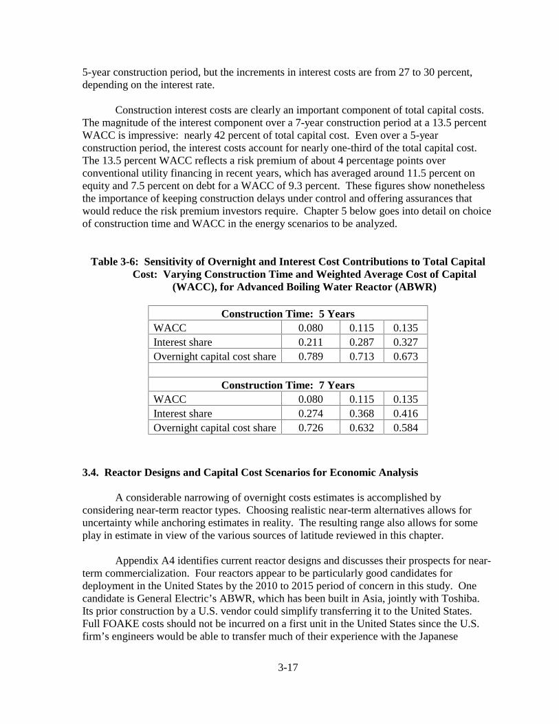
3-17

5-year construction period, but the increments in interest costs are from 27 to 30 percent,depending on the interest rate.

Construction interest costs are clearly an important component of total capital costs.The magnitude of the interest component over a 7-year construction period at a 13.5 percentWACC is impressive: nearly 42 percent of total capital cost. Even over a 5-yearconstruction period, the interest costs account for nearly one-third of the total capital cost.The 13.5 percent WACC reflects a risk premium of about 4 percentage points overconventional utility financing in recent years, which has averaged around 11.5 percent onequity and 7.5 percent on debt for a WACC of 9.3 percent. These figures show nonethelessthe importance of keeping construction delays under control and offering assurances thatwould reduce the risk premium investors require. Chapter 5 below goes into detail on choiceof construction time and WACC in the energy scenarios to be analyzed.

Table 3-6: Sensitivity of Overnight and Interest Cost Contributions to Total Capital Cost: Varying Construction Time and Weighted Average Cost of Capital

(WACC), for Advanced Boiling Water Reactor (ABWR)

Construction Time: 5 YearsWACC 0.080 0.115 0.135Interest share 0.211 0.287 0.327Overnight capital cost share 0.789 0.713 0.673

Construction Time: 7 YearsWACC 0.080 0.115 0.135Interest share 0.274 0.368 0.416Overnight capital cost share 0.726 0.632 0.584

3.4. Reactor Designs and Capital Cost Scenarios for Economic Analysis

A considerable narrowing of overnight costs estimates is accomplished byconsidering near-term reactor types. Choosing realistic near-term alternatives allows foruncertainty while anchoring estimates in reality. The resulting range also allows for someplay in estimate in view of the various sources of latitude reviewed in this chapter.

Appendix A4 identifies current reactor designs and discusses their prospects for near-term commercialization. Four reactors appear to be particularly good candidates fordeployment in the United States by the 2010 to 2015 period of concern in this study. Onecandidate is General Electric’s ABWR, which has been built in Asia, jointly with Toshiba.Its prior construction by a U.S. vendor could simplify transferring it to the United States.Full FOAKE costs should not be incurred on a first unit in the United States since the U.S.firm’s engineers would be able to transfer much of their experience with the Japanese

3-18

construction. Remaining engineering costs for a first U.S. plant can be assumed to beincluded in engineering and home office services, account 92. Another candidate reactor isthe CANDU ACR-700, which is a light water reactor that uses heavy water for moderation,manufactured by Atomic Energy Canada, Ltd (AECL). It is an advance on the CANDU 6,which has had several units built recently in China and Romania. AECL requested pre-application review for the ACR-700 by the U.S. Nuclear Regulatory Commission (NRC) inJune 2002, and NRC expects to complete the process by mid-2004. The ACR-700’s costcharacteristics appear to overlap that of the ABWR despite the size difference (1,350 MWversus 700 MW). The low estimate of overnight costs to be used in the uncertainty analysiswould represent either of these reactors. Although a CANDU reactor has not been built inthe United States, the extensive recent experience of AECL with the closely related CANDU6 could keep FOAKE costs for the ACR-700 in the United States relatively low. In theabsence of further information, those costs are assumed to be coverable within engineeringand home office services.

Still another candidate reactor is Westinghouse’s AP1000. It is a larger version of theAP600, whose design NRC has certified. Obtaining certification for the AP1000 should beaccelerated by the prior certification of its smaller version. Cost estimates for the AP1000were considered in detail in this chapter. This reactor represents a mid-range cost.

A final candidate reactor is Framatome’s Siede Wasser Reaktor (SWR) 1000, aboiling water reactor (BWR) which was considered seriously for construction in Finland. ItsBWR features have been proven in the European market, and Framatome has expressedintent to submit the SWR 1000 for design certification by the end of 2005 (Cushing 2002,NRC 2002, Mallay 2002, Sebrosky 2002). Its cost per kW is expected to parallel that ofFramatome’s EPR (Framatome ANP 2003; UIC 2004, p. 4), which has been selected for theproject in Finland, although Framatome has announced no plans for marketing that design inthe United States. The SWR 1000 represents a high-end cost (UIC 2003, p. 3).

These designs span a spectrum of characteristics while having realistic prospects fornear-term deployment in the United States.

The ABWR is a mature plant, the FOAKE costs on which have already been paid. Itsovernight cost is estimated at $1,246 per kW. The ACR-700’s construction times have beenshort, as little as 4.5 years from first pouring of concrete to criticality (NRC considers prioractivities as part of its lead time definition), and AECL’s projection of overnight costs havebeen as low as $985 to $1,000 per kW, although EIA (2004) suggests a cost of $1,100 to$1,200 per kW for the third construction of twin units, giving a cost similar to that of theABWR.

The AP1000 has not yet been built. The FOAKE costs are yet to be paid. On theassumption that the entire FOAKE cost is assigned to the first plant, this plant’s cost isspecified at $1,500 per kW, representative of the midrange overnight cost estimate.

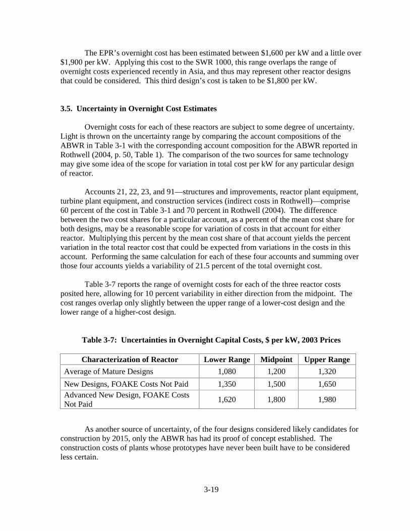
3-19

The EPR’s overnight cost has been estimated between $1,600 per kW and a little over$1,900 per kW. Applying this cost to the SWR 1000, this range overlaps the range ofovernight costs experienced recently in Asia, and thus may represent other reactor designsthat could be considered. This third design’s cost is taken to be $1,800 per kW.

3.5. Uncertainty in Overnight Cost Estimates

Overnight costs for each of these reactors are subject to some degree of uncertainty.Light is thrown on the uncertainty range by comparing the account compositions of theABWR in Table 3-1 with the corresponding account composition for the ABWR reported inRothwell (2004, p. 50, Table 1). The comparison of the two sources for same technologymay give some idea of the scope for variation in total cost per kW for any particular designof reactor.

Accounts 21, 22, 23, and 91—structures and improvements, reactor plant equipment,turbine plant equipment, and construction services (indirect costs in Rothwell)—comprise60 percent of the cost in Table 3-1 and 70 percent in Rothwell (2004). The differencebetween the two cost shares for a particular account, as a percent of the mean cost share forboth designs, may be a reasonable scope for variation of costs in that account for eitherreactor. Multiplying this percent by the mean cost share of that account yields the percentvariation in the total reactor cost that could be expected from variations in the costs in thisaccount. Performing the same calculation for each of these four accounts and summing overthose four accounts yields a variability of 21.5 percent of the total overnight cost.

Table 3-7 reports the range of overnight costs for each of the three reactor costsposited here, allowing for 10 percent variability in either direction from the midpoint. Thecost ranges overlap only slightly between the upper range of a lower-cost design and thelower range of a higher-cost design.

Table 3-7: Uncertainties in Overnight Capital Costs, $ per kW, 2003 Prices

Characterization of Reactor Lower Range Midpoint Upper Range

Average of Mature Designs 1,080 1,200 1,320

New Designs, FOAKE Costs Not Paid 1,350 1,500 1,650Advanced New Design, FOAKE CostsNot Paid

1,620 1,800 1,980

As another source of uncertainty, of the four designs considered likely candidates forconstruction by 2015, only the ABWR has had its proof of concept established. Theconstruction costs of plants whose prototypes have never been built have to be consideredless certain.

3-20

A statistical estimate of a reliability range, for overnight costs, for example a 90percent confidence range, could be estimated by performing a compound probability analysiscombining probability distributions of the three sources of uncertainty, namely uncertainty asto which technology will be used, uncertainty about for any given technology, anduncertainty due to the lack of proof of concept. To do so would require probability weightson values in each of the distributions. Normal central tendencies in each of the distributionsreduce the likelihood of extremely high or low values in any of the three distributions. Thelikelihood of extreme overnight cost values is further reduced when probabilities aremultiplied together to obtain an overall compound probability distribution of overnight costs.Lacking knowledge of the actual probability distributions and recognizing the tendency forprobabilities of midrange values to be higher than outlying values, it is hoped that the $1,200,$1,500, and $1,800 per kW estimate range used in this study represents a confidence intervalfor overnight capital costs associated with a higher degree of reliability.

3-21

References

Cushing, Jack. (2002) “Memorandum: Summary of Meeting with Framatome ANPRegarding the Design Certification Process for the SWR 1000.” New Reactor LicensingProject Office, Office of Nuclear Reactor Regulation, U.S. Nuclear Reactor Regulation.Rockville, Md, April 4. Retrieved December 2003 from World Wide Web:http://www.nrc.gov/reactors/new-licensing/new-licensing-files/ml020940471.pdf.

Delene, J. G., and C. R. Hudson II. (1993) Cost Estimate Guidelines for Advanced NuclearPower Technologies. ORNL/TM-10071-R3. Oak Ridge, Tenn.: Oak Ridge NationalLaboratory, May.

Electric Power Research Institute (EPRI). (2003) Nuclear Power’s Role in MeetingEnvironmental Requirements: Evaluation of E-EPIC Economic Analyses, EPRI 1007618.Palo Alto, CA: EPRI, January.

Energy Information Administration (EIA). (2004) Annual Energy Outlook 2004 (AEO2004). Washington, D.C.: U.S. Department of Energy, January. DOE/EIA-0383(2004).

Energy Information Administration (EIA). (2001) Assumptions to the Annual EnergyOutlook 2002 (AEO 2002). Washington, D.C.: U.S. Department of Energy, December.DOE/EIA-0554(2002).

Framatome ANP. (2003) “Framatome ANP Submits its Tender to Build a New NuclearUnit in Finland,” March 31. Retrieved December 2003 from World Wide Web:http://www.framatech.com/newsreleases/newsrelease.sap?NewsNumber=190.

Mallay, James F. (2002) Letter to Samuel J. Collins, Office of Nuclear Reactor Regulation,U.S. Nuclear Regulatory Commission. Lynchburg, Va, May 31. Retrieved December 2003from the World Wide Web: http://www.nrc.gov/reactors/new-licensing/new-licensing-files/2002-6-6-60276221.pdf.

Massachusetts Institute of Technology (MIT). (2003) The Future of Nuclear Power: AnInterdisciplinary MIT Study. Cambridge, Mass.: Massachusetts Institute of Technology,July.

Nuclear Energy Agency, Organization for Economic Co-Operation and Development (NEA).(2000) Reduction of Capital Costs of Nuclear Power Plants. Paris: OECD.

Paulson, C. Keith. (2002) “AP1000: Set to Compete,” Nuclear Engineering International47, Issue 579 (October): 20-22.

Reis, Victor H., and Matthew P. Crozat. (2002) “A Strategy for U.S. Nuclear Power: TheRole of Government.” Mimeo. Washington, D.C.: SAIC.

3-22

Rothwell, Geoffrey. (2004) “Triggering Nuclear Development,” Public Utilities Fortnightly142, No. 5: 46-51.

Sebrosky, Joseph M. (2002) “Memorandum: Summary of August 15, 2002, Meeting withFramatome ANP Regarding the SWR 1000.” New Reactor Licensing Project Office, Officeof Nuclear Reactor Regulation, U.S. Nuclear Reactor Regulation. Rockville, Md, September19. Retrieved December 2003 from Word Wide Web: http://www.nrc.gov/reactors/new-licensing/new-licensing-files/swr1000.pdf.

Uranium Information Centre (UIC). (2003) “Nuclear Energy in Finland.” Briefing Paper #76. Melbourne: UIC, December.

Uranium Information Centre (UIC). (2004) “The Economics of Nuclear Power.” BriefingPaper 8. Melbourne: UIC, March.

U.S. Department of Energy (DOE). (1988) Phase IX Update (1987) Report for the EnergyEconomic Data Base Program EEDB – IX. DOE/NE-0091. Washington, D.C.: AssistantSecretary for Nuclear Energy, Office of Program Support, Plans and Evaluation Division,July.

U.S. Department of Energy (DOE). (2001) “A Roadmap to Deploy New Nuclear PowerPlants in the United States by 2010, Volume II.” Main Report. Washington, D.C.: Office ofNuclear Energy, Science and Technology, October.

U.S. Nuclear Regulatory Commission (NRC). (2002) “Design Certification Pre-Application Review—SWR 1000.” Retrieved December 2003 from Word Wide Web:http://www.nrc.gov/reactors/new-licensing/license-reviews/design-cert/SWR 1000.html.

4-1

Chapter 4. LEARNING BY DOING

Summary

Reductions in capital costs between a first new nuclear plant and some nth plant of thesame design can be of critical importance to eventual commercial viability. In building theearly units of a new reactor design, engineers and construction workers learn how to buildnew nuclear plants more efficiently with each plant they build. This chapter examines theevidence of cost reductions for nuclear power plants contributed by learning. The findings ofthis chapter are used in Chapter 9 to estimate the reduction in LCOEs due to learning effectsthat would take place after construction of early nuclear plants, lessening and possiblyeliminating the need for government policies aimed at the nuclear power industry afterbuilding the first few plants.

A case can be made that the nuclear industry will start near the bottom of its learningcurve when new nuclear construction occurs. The paucity of any new nuclear construction inthe past twenty years in the United States, together with the entry of new technologies and anew regulatory system, has eliminated much of the applicable experience of the U.S. craftworkforce. Participation in overseas construction may have given some U.S. engineersexperience that is transferable to construction in the United States, but the internationalmobility of craftsmen is much less. Consequently, considerable learning is to be expectedduring the construction of the first few new plants.

Studies of nuclear plants built in the 1960s and 1970s report evidence of learningrates of 5 to 7 percent with doubling of plants constructed. Extending the sample of plants tothose built in the 1980s weakens the ability to identify construction learning effects. Studieshave found lower costs on plants built in-house by a utility itself rather than by a contractor,as much as 25 percent; but an earlier study found a 30 percent higher cost on in-houseconstruction. It is possible that the in-house effect is the result of contractors in a marketwith limited competition.

A plausible range for future learning rates in the U.S. nuclear construction industry isbetween 3 and 10 percent. Three percent is conservative. It is consistent with a scenarioinvolving low capacity growth, reactor orders of a variety of designs spaced widely enoughapart in time that engineering and construction personnel cannot maintain continuity, someconstruction delays, and a construction industry that can retain internally a considerableproportion of learning benefits. A medium learning rate of 5 percent is appropriate for ascenario with more or less continuous construction, with occasional but not frequent cases ofsequential units built at a single facility, a narrower range of reactor designs built by a morecompetitive construction industry, with delays uncommon. A 10 percent learning rate isaggressive. It would necessitate a continuous stream of orders that keep engineering teamsand construction crews intact, a highly competitive construction industry, and streamlinedregulation largely eliminating construction delays.

4-2

Outline

4.1. Introduction

4.2. What is Learning by Doing?

4.3. Learning by Doing as a General Phenomenon

4.4. Estimation Problems

4.5. Firm Learning by Doing

4.5.1. The Standard Approach4.5.2. Principal-Agent Framework and Firm Learning4.5.3. Learning by Doing Overseas

4.6. Industry Learning by Doing

4.7. Allowing for Other Factors Affecting Capital Costs

4.7.1. Regulation4.7.2. In-House Management4.7.3. Multiple-Unit Sites4.7.4. Economies of Scale and Construction-Time Effects4.7.5. Region

4.8. Forgetting and Knowledge Depreciation

4.9. Conclusion

References

4-3

4.1. Introduction

The purpose of this chapter is to draw lessons for the future from the historicalexperience of learning by doing. Section 4.2 defines learning by doing. Section 4.3 reportslearning rates in industries other than nuclear plant construction. Section 4.4 describesobstacles that hinder measuring learning by doing. Section 4.5 reviews the research on firmlearning rates: Section 4.5.1 considers the standard approach studies that sought only tomeasure learning by doing; Section 4.5.2 analyzes the later studies that sought to characterizelearning by doing in greater detail; and Section 4.5.3 looks at research comparing firmlearning in the United States with firm learning overseas. Section 4.6 evaluates the researchon industry learning by doing. Section 4.7 examines factors other than learning by doing thatseven studies found to be significantly related to nuclear power plant capital costs: regulation(4.7.1), in-house management (4.7.2), multiple-unit sites (4.7.3), economies of scale andconstruction-time effects (4.7.4), and region (4.7.5). Finally, Section 4.8 discussesknowledge depreciation, and Section 4.9 concludes by summarizing the factors influencingalternative learning rates.

4.2. What is Learning by Doing?

As a product is produced over and over, the marginal cost of producing it oftendecreases. When this decrease is not a result of economies of scale or a drop in input prices,it may be a result of learning by doing. Learning by doing occurs when the human beingsinvolved in a production process gain experience performing their tasks and, over time, findmore efficient ways to do them. Costs of production decrease until potential gains inefficiency from learning are exhausted, at which point the costs level off toward anasymptote.

Learning by doing is an observed phenomenon; theories exist about where in theproduction process the learning occurs, but they remain theories. Epple et al. (1991, p. 59)offer a list of factors contributing to learning by doing:

“Factors suggested as being responsible for organizational learning include: increased proficiency of individuals, including direct labor, management, and engineering staff; greater standardization of procedures; improvements in scheduling; improvements in the flow of materials; improvements in product design; improvements in tooling, layout, materials, and equipment; better coordination; division of labor and specialization; incentives; leadership; and learning by firms outside the focal firm, including suppliers and other firms in the industry.”

Moreover, learning rates probably capture the learning effects from multiple, differentagents within a firm: “The learning curve should be thought of as an aggregate model in thesense that it includes learning from all sources within the firm” (Yelle 1979, p. 309).Joskow and Rose (1985, p. 8) write:

4-4

“Any simple measure of experience represents at best a characterization of a very complicated process that is not yet well understood theoretically. In most studies on learning by doing, a researcher recognizes that costs of production have decreased in a given industry. He then collects data, controls for other factors, and if he finds a correlation between costs and the production firm’s experience, he concludes that learning by doing exists in that industry.”

Learning by doing is most often quantified by a learning rate. A learning rate is thepercentage decrease in cost each time cumulative output doubles. This definition of thelearning rate can be calculated by the power law. The cost of the nth unit produced isreduced, relative to the first unit produced, by a factor 2ln/ln)1( nd− , where d is the percentcost reduction associated with a doubling of units produced, expressed as a fraction, and n isthe unit for which this expression calculates the cost reduction. Learning by doing isexpressed in learning rates because most investigations of learning curves find that learningmakes its greatest impact when a production process is new: over time, learning by doingexhibits diminishing returns. The learning rate captures the diminishing returns byexpressing the cost decrease as a constant percentage reduction at increasingly-spaced-outmarkers, that is, at doubling points of cumulative production. Alternatively, learning bydoing is sometimes expressed in a progress ratio, which is simply 100 minus the learningrate. Thus, a 20 percent learning rate is equivalent to an 80 percent progress ratio.

4.3. Learning by Doing as a General Phenomenon

The first paper on learning by doing in a manufacturing process was written by T.P.Wright in 1936 on airframe production. In his pioneering article, Wright (1936) found that“the direct labor cost of manufacturing an airframe fell by 20 percent with every doubling ofcumulative output” (Hatch and Mowery 1998, p. 1462). According to Yelle’s (1979)comprehensive survey of learning-curve literature, nearly all of the subsequent research untilthe late 1960s concentrated on military applications (Yelle 1979, p.320). Yelle cites twostudies by Hirsch (1952 and 1956): “Hirsch, in a comprehensive study of seven differentmachines built by a single manufacturer… found that the individual [learning rates] rangedfrom 16.5 to 20.8 percent” (Yelle 1979, p. 305). Hirsch’s follow-up study found a range of16.5 to 24.8 percent. Yelle next cites a 1958 study by R. Cole, in which Cole found “verylittle difference in [learning rates] between different types of manufacturing studies(18 percent to 23 percent)” (Yelle 1979, p. 305).

Learning by doing generally exhibits diminishing returns. Yelle calls this phenomenaplateauing, and cites 1966 and 1971 studies by Baloff: “Baloff studied plateauing inmachine-intensive manufacturing. The study consisted of twenty-eight separate cases of newproduct and new process startups that occurred in five separate companies in four differentindustries. Heavy emphasis was on the steel industry. Plateauing was observed in 20 out of28 cases” (Yelle 1979, p. 306). Yelle detected an interesting trend in the learning-research:learning effects are greater in labor-intensive manufacturing processes than in machine-intensive processes. For example, a study by Hirsch found that “assembly [learning rates]

4-5

were approximately two times as large (25.6 percent versus 14.1 percent)” (Yelle 1979, p.306). The implication is that the more processes performed by human beings, the greater theopportunities to learn. Irwin and Klenow (1994) found in the semiconductor industry thatfirms learn three times more from their own cumulative production than from cumulativeproduction of other firms and that learning spills over as much between firms in the samecountry as between firms in different countries.

In the research on learning by doing in the nuclear plant construction industry,nuclear learning rates are generally lower than the 20 percent average of other industries.There are many possible reasons for this phenomenon. First, and most significantly, eachnuclear power plant is a unique project, making experience from previous projects lessrelevant. As McCabe writes, “Homogeneity maximizes the usefulness of past productionexperience… In contrast, power plant D&C involved designs that exhibited considerableheterogeneity, reducing the usefulness of past experience” (McCabe 1996, p. 357-358).Second, cost uncertainty (as a result of both regulation and heterogeneous plant designs) andcost-plus contracting may have reduced construction firm’s incentives to reduce costs. Third,experienced construction firms may have been realizing decreasing costs but charging thehigher market price (rent-capturing).

4.4. Estimation Problems

Long construction times and complex accounting practices are hindrances toestimating learning by doing. Because power plant construction projects last a number ofyears, complicated calculations are necessary to remove inflation and interest duringconstruction (IDC) from the nominal cost numbers reported by utilities. Zimmerman,Komanoff, and Paik and Schriver use previous research on the typical cash flow for a nuclearpower plant construction project to estimate the proportion of the reported nominal costsspent each year of construction (Zimmerman 1982, p. 301; Komanoff 1982, p. 316). Oncethe costs are broken down year-by-year, they use average interest rates to subtract theappropriate interest and inflation.

Cantor and Hewlett, however, are critical of the use of both the typical cash flowmodel and average interest rates. They claim that the cash flow model is inaccurate andintroduces a bias correlated with time, leading “one to question the results of the otherresearch, since all the variables of interest are correlated with time” (Cantor and Hewlett1988, p. 323). Cantor and Hewlett claim to solve both problems by collecting accurateallowance for funds used during construction (AFUDC) and IDC rates from form FERC-1:“reported AFUDC rates collected from Form FERC-1 and supplemented by informationfrom various State public utility commissions to incorporate important accountingconventions are used to derive effects AFUDC rates” (Cantor and Hewlett 1988, p. 334).

Accounting practices present another barrier to calculating costs precisely: whenmultiple units are built at one site, utilities often allot a disproportionate fraction of sharedcosts to one of the units (Komanoff 1981, p.201; McCabe 1996, p. 365). Various methods

4-6

exist to control for this practice, which are discussed in Section 4.7.3. Most studies include adummy variable in the regression (see column “multiple” in Table 4-1). Komanoff (1981)averages total costs over units at the site. Regardless of the method of dealing with it, thelong construction times and thorny accounting practices involved in nuclear power plantconstruction projects make it difficult to calculate overnight capital costs. A comparison ofdata bases verified this: different studies calculate notably different overnight costs for thesame plants.

Moreover, experience can be difficult to measure. Most studies use either reactorscompleted by a firm or reactor-years, that is, years a firm spent building a reactor. Usingreactors completed by an architect-engineer “assumes learning takes place only aftercompletion,” while using reactor-years “assumes that completing a reactor in ten years isworth more than completing one in eight” (Zimmerman 1982, p. 300). Industry experience isespecially difficult to quantify using regression analysis, as it is highly correlated with thetime variable used in most regressions (Cantor and Hewlett 1988, p. 318).

The problem of precision is compounded when learning rates are used to modelfuture plant construction costs; a small difference in calculated learning rate can meansignificant differences in costs. McDonald and Schrattenholzer imagine a hypotheticaltechnology and find that “decreasing the learning rate from 20 percent to 10 percent wouldincrease technology maturing costs from $2 billion to $16 billion, and the break-evencapacity from 9 to 96 GW” (McDonald and Schrattenholzer 2001, p. 256).

4.5. Firm Learning by Doing

The first attempts at quantifying learning by doing in nuclear power plantconstruction tried only to establish whether learning by doing existed and to measure it.Later studies had more specific goals, such as testing for the impact of industry structure orcontract type on learning rates. McCabe thus calls the procedure of the early attempts thestandard approach (McCabe 1996, p. 358). Section 4.5.1 deals with these early studies andSection 4.5.2 describes the later studies.

4.5.1. The Standard Approach

Table 4-1 summarizes the regression equations of five of these initial efforts atmeasuring learning by doing. These five studies are quite similar, and thus are easy tocompare. Most of the regressions include variables for size, vintage, and firm experience,and dummy variables for whether the unit is the first at the site, whether a cooling tower wasbuilt, whether the project was managed by the utility (in-house), and what region where theplant was built. Vintage is generally used in these statistical analyses to capture the effects ofincreased regulation. The five studies in Table 4-1 also use data from similar time periods.The table also gives sample size, r2 value, and estimated learning rate for each study.

4-7

Tab

le 4

-1:

Sum

mar

y of

Reg

ress

ion

Ana

lyse

s of

Lea

rnin

g by

Doi

ng in

Nuc

lear

Pow

er P

lant

Con

stru

ctio

n

Pap

er/D

atab

ase

Size

Cos

tSi

zeD

ate/

Vin

tage

Exp

erie

nce

Exp

erie

nce2

Mul

tipl

eC

oolin

g T

ower

In-H

ouse

Reg

ions

Oth

er V

aria

bles

Moo

z 19

79ln

(c

per

kW)

SIZ

EC

PIS

LN

TO

WE

R

LO

C1

BW

T1R

SID

and

T2R

SID

54 p

lant

s is

sued

perm

its th

roug

hD

ecem

ber

1972

; r2 =

0.67

; lea

rnin

g ra

te =

11.2

per

cent

IDC

incl

uded

insi

gnif

ican

tD

ate

cons

truc

tion

perm

it is

sued

Nat

ural

log

ofcu

mul

ativ

enu

mbe

r of

LW

Rpo

wer

pla

nts

byar

chite

cten

gine

er

dum

my;

insi

gnif

ican

t

Dum

my;

1 if

Nor

thea

st, 0

ifot

her

Bab

cock

-Wilc

oxm

anuf

actu

red

the

NSS

S; in

sign

ific

ant

resi

dual

s fr

om a

noth

erre

gres

sion

; ins

igni

fica

nt

Paik

and

Sch

rive

r19

79ln

Cln

(M

W)

ln

N

D

1-D

4R

IR

I^2

65 p

lant

s is

sued

perm

its b

etw

een

1967

and

1974

and

whi

chw

ere

com

plet

ed o

rex

pect

ed to

be

com

plet

ed b

y 19

81;

r2

= 0.

78; l

earn

ing

rate

=21

.9 p

erce

nt

IDC

incl

uded

cum

ulat

ive

num

ber

of L

WR

plan

ts b

uilt

byde

sign

fir

m

dum

my

was

incl

uded

inre

gres

sion

, but

resu

lts w

ere

insi

gnif

ican

t

of

fou

r re

gion

s,on

ly tw

o(u

nspe

cifi

ed)

regi

onal

dum

mie

sw

ere

sign

ific

ant

"Reg

ulat

ion

Impa

ctIn

dex:

" E

ach

regu

lati

on w

asas

sign

ed a

n im

pact

ratin

g (1

-4);

Sum

of

regu

lati

ons

in y

ear

of c

onst

ruct

ion-

>

used

alg

orith

m to

est

imat

eim

pact

of

regu

latio

ns d

urin

gco

nstr

uctio

n

Kom

anof

f 19

81ca

pita

l cos

t, K

MW

CU

MU

LA

TIV

EN

UC

LE

AR

CA

PA

CIT

Y

A-E

M

UL

TIP

LE

CO

OL

ING

TO

WE

R

NO

RT

HE

AST

DA

NG

LIN

G

note

: on

ly s

tati

stic

ally

sign

ific

ant v

aria

bles

give

n in

stu

dy;

46re

acto

rs c

ompl

eted

betw

een

Dec

embe

r19

71 a

nd D

ecem

ber

1978

; r2 =

0.92

3;ad

just

ed r

2 = .9

08;

lear

ning

rat

e =

7pe

rcen

t

$ pe

r K

W,

with

out

estim

ated

ID

C;

used

cos

tsfr

om d

ata

repo

rted

"ye

arfo

llow

ing

com

mer

cial

oper

atio

n"(p

.198

)

ca

ptur

es e

ffec

t of

regu

lati

onnu

mbe

r of

reac

tors

bui

lt by

arch

itect

-en

gine

er

du

mm

y; 1

ifun

it is

par

t of

am

ultip

le-u

nit

site

, 0 if

uni

t is

stan

d-al

one

dum

my

ran

sepa

rate

regr

essi

on to

test

for

inho

use

effe

cts

only

nor

thea

stre

gion

had

sign

ific

ant c

ost

diff

eren

ce

succ

esso

rin

com

plet

e at

tim

eof

stu

dy; K

. una

ble

to a

vera

ge c

osts

acro

ss r

eact

ors

atsi

te

Zim

mer

man

198

2lo

g ac

tual

cos

t,kw

SIZ

EY

EA

R1

(1/(

1+E

XPF

)(1

/(1+

EX

PI)

FIR

STT

SEL

FC

OR

7-R

11L

ET

IME

LU

TIM

E

41 p

lant

s co

mpl

eted

betw

een

1968

and

1980

; r2 =

0.8

5;le

arni

ng r

ate

inT

able

3

per

kilo

wat

t in

1979

$,re

mov

edes

timat

ed I

DC

;

in M

Win

whi

ch n

ucle

arde

cisi

on w

asan

noun

ced

expe

rien

ce(c

ompl

eted

reac

tors

) of

cons

truc

tion

firm

; mea

sure

spr

ivat

e le

arni

ng

cum

ulat

ive

indu

stry

expe

rien

ce;

exte

rnal

ityas

soci

ated

with

cons

truc

tion

activ

ity

dum

my;

1 if

firs

t uni

t at

site

, 0 if

othe

rwis

e

dum

my;

1 if

mec

hani

cal

cool

ing

tow

er

dum

my;

1 if

cons

truc

tion

was

don

e by

utili

ty

5 re

gion

slo

g of

the

num

ber

of y

ears

ori

g.an

ticip

ated

bet

wee

nan

noun

cem

ent a

ndop

erat

ion

log

of th

e di

ff. b

etw

een

actu

al a

nd a

ntic

ipat

ed ti

me

toop

erat

ion

Can

tor

and

Hew

lett

1988

ln (

c pe

r kW

)ln

(SIZ

E)

CO

NST

RT

CST

1

FIR

STC

OO

LB

UIL

DIP

RIC

Eln

(co

nstr

uctio

ntim

e)IN

TE

R

67 p

lant

s w

ithsc

hedu

led

com

mer

cial

oper

atio

n be

fore

198

6;ad

just

ed r

2 =0

.85;

lear

ning

rat

e =

lear

ning

coe

ffic

ient

insi

gnif

ican

t

"use

act

ual

AFU

DC

rat

esan

d ca

shpr

ofile

s" to

rem

ove

IDC

nu

mbe

r of

day

sbe

twee

n da

te o

fco

nstr

uctio

n st

art

and

1/1/

1960

(1/1

+EX

PF)

whe

re E

XPF

isnu

mbe

r of

com

plet

edre

acto

rs b

y"c

onst

ruct

or"

du

mm

y; 1

ifun

it is

a f

irst

or s

ingl

e un

itpl

ant

dum

my

dum

my;

1 if

utili

ty w

asco

nstr

uctio

nm

anag

er

cons

truc

tion

labo

rw

age

rate

in th

epl

ant’s

sta

te

ran

sepa

rate

regr

essi

on to

capt

ure

"ind

irec

t"ef

fect

s of

var

iabl

esth

roug

h ch

ange

s in

cons

truc

tion

tim

e

inte

ract

ive

term

bet

wee

nB

UIL

D a

nd C

ST1

4-8

Mooz (1979) studies 54 power plants with construction permits issued throughDecember 1972. Using regression variables for plant size, construction permit issue date,architect-engineer experience, use of a cooling tower, region, and manufacturer, he obtainsan r2 of 0.67, the lowest of the five standard-approach studies. This is partly because onlythree of his variables are statistically significant: construction permit issue date, architect-engineer experience, and Northeast location. The significance of architect-engineerexperience in Mooz’s regression indicates that learning by doing does exist in nuclear plantconstruction, but there is reason be wary of the precision of the coefficient.

First, the coefficients for use of a cooling tower and for size of the plant areinsignificant. Most later studies find significant cost effects related to size, as discussed inmore detail in Section 4.7.4, and nearly all but Mooz find a significant cost increase relatedto the use of a cooling tower (Mooz himself considers this lack of significance puzzling).Second, Mooz does not control for whether or not a nuclear unit was part of a multi-unit siteor whether the utility managed construction, and he only controls for one region, theNortheast. As Table 4-1 shows, later studies control for these factors and obtain moresatisfactory results. Mooz’s data base includes several cost estimates (as opposed to costreports), and he does not try to remove interest during construction from reported capitalcosts. By using cost numbers with interest during construction included, Mooz biases hiscost calculations against plants that took longer to build. All said, Mooz calculates a firmlearning rate of 11.2 percent. Nonetheless, his study paved the way for later studies ofnuclear plant capital costs, and it does find learning effects.

Paik and Shriver (1979) perform an analysis very similar to Mooz’s, using 65 plantswith permits issued between 1967 and 1974. Paik and Schriver’s regression include the samevariables as Mooz’s, but with two major differences: Paik and Schriver use total costs, notcosts per kW, as the dependent variable, and they use a regulation impact index (explained inSection 4.7.1) instead of a vintage variable (vintage is usually used a proxy for the effects ofregulation) (Paik and Schriver 1979, p. 230). With an r2 of 0.78, Paik and Schriver’sregression explains a great deal more of the variance in capital costs than does Mooz’s.However, it cannot be assumed that Paik and Shriver’s calculation of the learning rate isprecise, for the same reasons cited regarding Mooz’s results. Like Mooz, Paik and Schriverdo not find significant cost effects from the existence of a cooling tower, while the laterstudies all found significant effects.

Also like Mooz, Paik and Shriver do not include a variable to control for either first-unit status or in-house construction and do not remove interest during construction fromreported capital costs. Moreover, the cost numbers for several of the last plants in Paik andSchriver’s database are only estimates – construction had not yet been completed. This lastfactor potentially explains Paik and Shriver’s relatively high learning rate estimate of21.9 percent: realized costs in nuclear plant construction often overran estimated costs;using only cost estimates for later plants could make it appear that costs were decreasing overtime. Overall, Paik and Schriver’s study is similar to Mooz’s and is open to the sameconcerns.

4-9

Komanoff (1981) studies capital costs of both nuclear and coal power plants.Employing a nuclear data base of 46 reactors completed between December 1971 andDecember 1978, Komanoff estimates a regression using variables for architect-engineerexperience, size, cumulative nuclear industry capacity, and dummy variables for multi-unitsite, dangling status, region, and use of a cooling tower (Komanoff 1981, p. 198). Utilitiesoften allocate costs for plants at multi-unit sites unevenly. Komanoff solves this byaveraging total costs over the number of units at a site; dangling status means not all the unitsat a multi-unit site were complete at the time of the study, making averaging impossible(Komanoff 1981, p. 201). Komanoff’s study is a departure from the previous two studies inseveral respects. First, he controls for multi-unit sites, while Mooz and Paik and Schriver donot, and found significant cost reductions for reactors at such sites. By controlling fordangling status, Komanoff prevents disproportionate cost allocations at multi-unit sites frombiasing the results against incomplete multi-unit sites.

Second, Komanoff’s cost numbers better represent the overnight capital costs ofbuilding a plant: he removed estimated interest during construction from reported costs, andused costs reported in the year after the plant came online to capture substantial first-yearcapital costs (Komanoff 1981, p. 198). These techniques, together with Komanoff’s highadjusted r2 of 0.908 and high significance of the learning coefficient (> 99.9 percent), givehis estimated firm learning rate of 7 percent appear statistically reliable. He also finds that“the 95 percent confidence interval ranges from between a 5 and 9 percent cost reduction foreach doubling of experience” (Komanoff 1981, p. 200). However, Zimmerman’s 1982 studyand Cantor and Hewlett’s 1988 studies (below) give reason to question these results.

Zimmerman studies 41 plants finished between 1968 and 1980 “for which completedcost figures are available” (Zimmerman 1982, p. 301). He uses variables for size, vintage,anticipated construction time, difference between anticipated and actual construction times,construction firm experience, industry experience, and dummy variables for use of a coolingtower, first-unit status, region, and in-house construction (Zimmerman 1981, p. 299).Zimmerman’s study is most comparable with Komanoff’s, mainly because both use a cash-flow model to remove estimated IDC from reported costs (Mooz and Paik and Schriver donot remove IDC, while Cantor and Hewlett use actual cash-flow data).

Although Zimmerman’s study is most similar to Komanoff’s, Zimmerman’sregression differs from Komanoff’s in several respects. First, while Komanoff usescumulative nuclear industry capacity to capture the effects of regulation, Zimmerman uses atime variable. Second, Zimmerman includes regression variables for anticipated and actualconstruction time, in-house construction, and industry learning effects, while Komanoff doesnot. Third, Zimmerman uses an alternate form of the experience variable, 1/(1 + experience),instead of simple experience (Zimmerman 1982, p. 300). The effects of these threedifferences on the accuracy of results are ambiguous; most of Zimmerman’s additionalvariables are statistically significant. Zimmerman’s use of the 1/(1 + experience) form of theexperience variable makes calculating a constant learning rate impossible. While thelearning rate is a constant percent reduction for each doubling of experience, Zimmerman’s

4-10

form of the experience variable results in decreasing percent reductions at each doublingpoint of experience. That is, a learning curve using Zimmerman’s functional form exhibitsmore sharply diminishing returns from learning than a standard exponential curve. Table 4-2shows how using Zimmerman’s functional form results in decreasing percent reductions ateach doubling point of experience. Table 4-2 also compares Zimmerman’s results usingcumulative completed plants as the experience measure with his results using cumulativereactor-years: “for example, a reactor under construction for five years represents fivereactor-years” (Zimmerman 1982, p. 300). Zimmerman’s results resemble Komanoff’s; fromZimmerman’s data, a constant average learning rate (constant percent reduction) of 5 percentmight be approximated. The firm learning coefficient in Zimmerman’s regression issignificant at over the 99.9 percent level. Learning effects are calculated by the power lawexpression in this study rather than by Zimmerman’s variant, because the former calculationis the conventional approach.

Table 4-2: Zimmerman’s Learning Effects

Experience Measure: Completed PlantsChange in Constructor Experience Percent Cost Decrease

1�2 7.42�4 5.94�8 4.08�16 2.7

Experience Measure: Reactor-YearsChange in Constructor Experience Percent Cost Decrease

1�2 8.02�4 6.54�8 4.58�16 2.7

Source: Zimmerman (1982).

Zimmerman makes an important point about calculated firm learning effects:

“There is a potentially large bias in the estimate of internalized [firm] learning effects. A construction firm with a great deal of experience can capture rents. Such a firm can charge the price of its competitors and realize the lower cost as profit.The utility is not without bargaining power, and a likely outcome is a sharing of the rent” (Zimmerman 1982, p. 304).

That is, a construction firm may be realizing lower costs as it gains experience, butbecause the firm can charge the price of its less-experienced competitors, this learning effectis only partially represented in the prices paid by the utilities. This would introduce adownward bias in learning rate estimates, even if the relation of the learning to the cost paid

4-11

by the utility is accurately reflected in the estimated learning coefficient. Zimmerman notesthat including a regression parameter for in-house construction can help determine the extentof this bias: if utilities that manage their own construction realize lower costs than those thatoutsource to a construction firm, it may be evidence that construction firms are chargingprices significantly above costs. He finds that on average, in-house construction resulted in22 percent lower costs (Zimmerman 1982, p. 303). This saving may indicate thatconstruction firms were capturing rents (in which case, calculated learning rates are biaseddownward, but still accurately indicate utilities’ cost savings), or it may simply indicate thatutilities run construction projects better. Zimmerman says of the lower costs for in-houseconstruction: “This could reflect savings due to a better managerial arrangement, or it couldindicate that in these cases the utility captured the entire rent” (Zimmerman 1982, pp. 304-305). In sum, rent-capturing may be pushing calculated learning rates downward, but thatcannot be certain.

This consideration suggests a first reason to question the reliability of Komanoff’sresults: whereas Komanoff finds that in-house construction led to 30 percent higher capitalcosts, Zimmerman finds that in-house construction resulted in 22 percent lower costs.(Komanoff 1981, p.200; Zimmerman 1982, p. 303). Komanoff does not include a variablefor in-house construction in his main regression. However, he estimates a separateregression to test for in-house effects: “The result was a 30 percent higher cost for self-A-E,with a 95 percent confidence interval of 13 to 50 percent and a 99.9 percent significancelevel” (Komanoff 1981, p. 200). Furthermore, Cantor and Hewlett’s results agree withZimmerman’s (Cantor and Hewlett 1988, p. 332). This may be a result of different databases, although Zimmerman’s (1968-1980) brackets Komanoff’s (1971-1978) in time.

Alternatively, it may be a result of regression techniques or cost deflation data – it isdifficult to tell without access to Zimmerman’s data (Komanoff provides his). The pointworth noting, however, is that the two authors examining similar time periods can findwidely disparate cost effects from a given factor. Moreover, Komanoff’s in-house effectcoefficient is significant at the 99.9 percent level – the same high significance level of thelearning effects he finds. This must be taken into account when considering Komanoff’s7 percent learning rate.

Cantor and Hewlett’s study includes 67 nuclear plants “with scheduled commercialoperation before 1986” (Cantor and Hewlett 1988, p. 322). Their regression includesvariables for size, construction labor wage rate in the plant’s state (a proxy for regional costdifferences), construction time, vintage, constructor experience, and dummy variables for useof a cooling tower, first-plant (at a multi-unit site) or single-plant status, and in-houseconstruction. They also include an interactive term between constructor experience and in-house construction. This study is a departure from the previous studies mainly in itsmethodology for estimating overnight costs. Where Komanoff and Zimmerman uses averagedebt rates and cash-flow models, Cantor and Hewlett use “actual AFUDC rates and cashprofiles” (Cantor and Hewlett 1988, p. 319). In a regression with an adjusted r2 of 0.85,Cantor and Hewlett find no learning effects for construction firms; they find “someevidence” of learning effects for utilities that managed construction themselves (Cantor and

4-12

Hewlett 1988, p. 330). This may be a result of a data base that includes plants from the1980s: Komanoff found regressions with nuclear plants built in the 1980s to be unstable(Komanoff, personal communication August 2003). It may also be a result of the rent-capturing bias—when construction firms realize lower costs as a result of experience, butcharge the higher market price because they can. This rent-capturing explanation fits wellwith Cantor and Hewlett’s findings of learning effects for in-house construction, in whichthere is no rent-capturing. Alternatively, Cantor and Hewlett may find no firm learningeffects because of their unique capital cost methodology, an explanation they favor.

According to Cantor and Hewlett, “it is very likely that the method used in theprevious research introduced measurement error into the dependent variable that is correlatedwith time” (Cantor and Hewlett 1988, p. 318). That is, the degree to which the average debtrates and cash-flow models were inaccurate changed over time. If this is true, thenKomanoff and Zimmerman may be finding some cost effects from variables correlated withtime (experience, for example) where there are, in fact, none. Indeed, Cantor and Hewlettthink that this might explain why their regression finds no firm learning effects whileKomanoff’s and Zimmerman’s do. This suggests another problem with Komanoff’s results.Cantor and Hewlett estimate a regression using the differences between their derivedovernight costs and Komanoff’s derived overnight costs as the dependent variables:“Although the sample contained only 28 units, we found evidence that the bias is positivelycorrelated with the experience variable. This would tend to explain the difference in results”(Cantor and Hewlett 1988, p. 330). That is, because Komanoff’s derived cost numbers wereoff by different degrees over time, his cost-calculation methodology may create theappearance of a learning curve where none exists.

Canterbery et al. (1996) conducted a regression analysis of determinants of cost perkW for 53 nuclear plants built in the United States. They employ a particularly parsimoniousspecification, using only four independent variables: the plant size, the duration of theproject, a regulatory variable, and a firm-level experience variable. The experience variabledefined as the number of nuclear projects owner-operated by the utility prior to constructionstart. They estimate a 13 percent doubling rate.

In summary, Mooz’s work, although pioneering, has reliability problems. Paik andSchriver also lack some of the techniques developed by the later studies. At first glance,Komanoff’s results seem very reliable, especially considering that Zimmerman finds asimilar learning effect for a similar period. However, Komanoff and Zimmerman findopposite effects for in-house construction, pointing to the sensitivity of statistical analyses ofsuch complex, lengthy construction projects. Cantor and Hewlett find evidence thatKomanoff’s and Zimmerman’s deflation methodology may have created the appearance oflearning effects where there are none. Keeping in mind that rent-capturing may bias learningrate calculations downward, the standard approach to this research implies that the learningrate for nuclear power plant construction could range from 0 to 10 percent.

4-13

4.5.2. Principal-Agent Framework and Firm Learning

McCabe studies 90 nuclear units finished by the end of 1988 (McCabe 1996, p. 368).His study differs from the standard approach studies in that he used a model of learning thatrelies on a principal-agent framework (McCabe 1996, p. 357). The principals (the utilities)outsource construction projects to the agents (the design and construction firms), except inthe case of in-house construction. McCabe recognizes a trend in the results of the standardapproach studies: in-house construction projects were generally cheaper than their agent-managed counterparts, and in-house construction exhibited greater learning effects (McCabecites Cantor and Hewlett’s 1988 study). Consequently, McCabe separates projects intoutility-managed and agent-managed groups to test whether utility- and agent-managers faceddifferent incentives (McCabe 1996, p. 358). He hypothesizes that cost-plus contracts andcost uncertainty (mainly as a result of an unstable regulatory environment) reduced theincentives to learn for agent-managers. He does not deal with Zimmerman’s rent-capturinghypothesis, that construction firms had profit as an incentive to reduce costs. McCabe furtherclassifies the agent-managed projects by length of the principal-agent relationship to testwhether longer relationships provide greater learning opportunities by allowing agents tobetter understand a utility’s unique design preferences. Additionally, McCabe notes thatbecause a utility that repeatedly manages construction in-house is essentially in a long-termrelationship with itself, “In-house utilities building a series of plants should also experiencerelatively larger learning benefits” (McCabe 1996, p. 361).

McCabe’s results generally conform to those of the standard-approach studies. In hisfirst regression, McCabe uses the standard approach: one experience coefficient representedthe experience of the unit’s architect-engineer. This regression shows no significant learningeffects. In his second regression, McCabe separates the experience variable into agentexperience (which takes a value of 1 if the agent managed construction), principal experience(which takes a value of 1 if construction was managed in-house), and specific-relationshipexperience (which takes a value of 1 if an agent had previously contracted with the utility).With an adjusted r2 of 0.87, the results indicate that in-house construction experience had alarger impact on in-house construction costs than agent experience had on agent-managedprojects (McCabe 1996, p. 372). In fact, McCabe finds that for utilities, each in-houseproject reduced the cost of the subsequent in-house project by 11.6 percent, while forarchitect-engineers, that number is 2 percent (McCabe 1996, p. 371). These percentages arereductions after every project, and therefore not learning rates for doubling; roughlycomparable learning rates would be about 30 percent for in-house and 6 percent for agent-managed. McCabe’s approximation of learning effects assumes constant returns fromlearning, but nearly all the research on learning by doing finds diminishing returns. Hisregression results, however, advance the understanding of learning as they reveal evidence ofconsiderably greater learning effects for utilities that manage projects in house. McCabe alsofinds specific-relationship experience insignificant, implying that “poor incentives rather thandesign variation account for the difference between agent and in-house procurement”(McCabe 1996, p. 372). That is, if design variation were responsible for the differencebetween in-house and agent-managed project costs, significant cost effects should be

4-14

observed in long-term relationships in which an agent can better understand its principal’sdesign preferences.

In summary, McCabe’s results give evidence that the extent of learning effectsdepends on incentives: in-house construction exhibits greater learning by doing becauseutilities have greater incentive to reduce cost than construction firms do. However,McCabe’s results could also support Zimmerman’s rent-capturing hypothesis: perhapsconstruction firms exhibit less substantial learning effects because they are charging pricesabove their costs. It is clear that estimations of future learning rates should take marketstructure into account, specifically, who will be managing plant construction and theincentives agent-managers face.

4.5.3. Learning by Doing Overseas

This section reviews learning by doing in overseas nuclear power plant constructionand considers the issue of transferring experience gained in recent overseas construction tofuture U.S. construction.

France’s nuclear energy program is known for its standardization. Thomas (1988)writes that France’s program was “the largest attempt at thorough-going standardization ofpower station design” (Thomas 1988, p. 195). The success of France’s program is widelyattributed to its efforts to standardize and modularize its nuclear reactors. Theoretically,learning by doing should thus exist to a higher degree in France than in the United States. Byproducing identical nuclear plants in series, France ensured maximum relevancy of pastexperience. “Standardization… makes it easier to identify empirical irregularities that pointto underlying structural conditions deserving further investigation. Therefore, it promotesthe learning process directly and widens the sphere of application for what has been learned”(David and Rothwell 1996, p. 191). Although there is a near consensus that France’sstandardization was both a catalyst in learning by doing and the reason for the French nuclearindustry’s success, capital cost studies on par with those focusing on the U.S. industry havenot been found. This may be a result of lack of adequate data; Thomas writes that Electricitéde France (EdF) releases data in a very global and aggregative form without specifying theextent of government subsidies: “This means that the absolute level of French constructioncosts must be treated with some care, if not suspicion, even for comparisons within France”(Thomas 1988, p. 232).

There is, however, evidence that France benefited from its standardization. Lesterand McCabe (1993) used plant operation data and Thomas used construction times toevaluate the French nuclear program. Lester and McCabe found that “the equivalentavailability factor”… increased more significantly in French plants than in U.S. plants,implying that the French learned how to effectively operate their plants sooner and to agreater degree than U.S. utilities learned to operate theirs (Lester and McCabe 1993, p. 435)."The equivalent availability factor is defined as the total amount of energy that a plant couldhave generated during the course of the year had it been called on to operated continuously atfull power, divided by the maximum annual energy output at continuous full-poweroperation” (Lester and McCabe 1993, p. 420). Moreover, in the United States, “Inter-reactor

4-15

learning (both within and among firms) is observed only when reactors of the same class areinvolved,” implying that learning effects are more significant when plants are similar oridentical. Examining construction times of French reactors, Thomas noted that althoughconstruction times did not decrease from 1971 to 1980, “Even more striking… is the fact thatconstruction times have not risen over time” (Thomas 1988, p. 229). That is, in contrast tothe U.S. and German experiences, and despite the fact that the French industry wasundergoing “very rapid expansion,” French construction times remained relatively constant.“There is little evidence of learning leading to reduction in construction times but this is atleast in part explained by the rather short schedules that the French programme establishedfrom the beginning” (Thomas 1988, p. 232). Furthermore, a 1984 article in Nucleonics Weekcites a study by the Electric Power Research Institute (EPRI), which found that French plantsrequired “50 percent or less of the electric and mechanical (craft) labor consumed by the U.S.plants studied” (MacLachlan 1984, p. 2). In summary, Lester and McCabe found that theFrench industry realized greater learning effects in operation and maintenance, while Thomasfound that France was able to avoid significant construction delays; the EPRI study foundthat French plants required significantly less labor to construct. All the studies explicitlyattribute their findings to France’s standardization and single-utility industry structure.

Japan’s nuclear industry has also been characterized as successful. In a 1988 article,Navarro attributes Japan’s success to standardization and a unique anti-trust policy. TheJapanese Ministry of International Trade and Industry (MITI) guided Japan into a two-designreactor program. The program was designed to reap the benefits of both standardization(reduced costs, greater learning effects) and competition (pressure to keep costs down). Ofstandardization, Navarro writes, “Besides the benefits associated with construction timereductions, these programs are generally credited with helping Japanese utilities raise theaggregate nuclear capacity factor from a low of 37 percent in 1977 to close to 80 percenttoday” (Navarro 1988, p. 9). However, Navarro notes that in a statistical analysis, he wasunable to find any firm-specific learning effects in Japan. Navarro attributes this lack of firmlearning to the prevalence of industry learning: “This important result suggests that thevarious Japanese consortia have been able very quickly to assimilate and share thetechnological stock of knowledge necessary to build nuclear plants” (Navarro 1988, p. 7).Navarro goes on to describe Japan’s unique anti-trust policy, writing that the Japanesegovernment “encourages cooperation and concentration within industries and views resultantconsortia as warriors in the international arena” (Navarro 1988, p. 9). Lastly, Navarro notesthat Japan’s “open and shut” licensing process allows Japanese utilities to pay lowerinsurance premiums on their capital (Navarro 1988, p. 10).

Although both the French and Japanese nuclear industries were relatively successful,a direct link between their success and their efforts to standardize remains unproven.Nonetheless, there is evidence implying that standardization leads to greater learning effects.A study by Kouvaritakis et al. (2002) estimates a 5.8 percent learning rate for OECD nuclearconstruction over the period 1975-1993 (reported in McDonald and Schrattenholzer 2001,Table 1, p. 257).

4-16

4.6. Industry Learning by Doing

Measuring industry learning by doing is more difficult than measuring firm learningby doing. Any measure of industry-wide experience is highly correlated with the timevariable, making it difficult to separate the two effects statistically. Firm experience alsocorrelates with time, although not so much so. However, what makes firm learning by doingsimpler to measure than industry learning by doing is that while costs are negativelycorrelated with firm experience (more experience leads to lower costs), costs generally arepositively correlated with industry experience (more experience seems to lead to highercosts). This effect is a result of increased regulation over time. Any measure of industryexperience increases with time, and as time passes, regulations increase, making it moredifficult and costly to build a plant. A statistical analysis will thus make it appear as ifgreater industry experience leads to higher costs. For example, while the industry might have30 more plants under its belt in 1980 than in 1970, a plant built in 1980 will cost more.Indeed, Komanoff used cumulative industry capacity as a proxy measure of regulationeffects.

4.7. Allowing for Other Factors Affecting Capital Costs

This section reviews the factors other than experience that researchers found to besignificantly correlated with nuclear plant capital costs: regulation (4.7.1), in-housemanagement (4.7.2), multiple-unit sites (4.7.3), economies of scale and construction-timeeffects (4.7.4), and region (4.7.5).

4.7.1. Regulation

To capture the effects of regulation, the most common technique has been to includea vintage variable. The cost in constant dollars of U.S. nuclear plants rose over the 1970sand 1980s, and the consensus among the studies is that this increase is mainly a result ofincreased environmental and safety regulation. Stricter standards “added significantly to theamounts of labor, materials, and equipment required to build reactors” (Komanoff 1981,p.202). The cost effects from regulation were compounded by the fact that regulations“frequently were mandated during construction, causing changes in design requirements thatmade it difficult for utilities to control schedules and costs” (Komanoff 1981, p. 202). Thestudies on plant costs go into little detail about what effects other than regulation the time-trend could be capturing; McCabe suggests changes in construction efficiency, but says littlemore (McCabe 1996, p. 366).

Table 4-3 shows the results of the studies. Nearly all the studies find that costs inconstant dollars rose between 10 to 24 percent each year after all other factors have beencontrolled. First, note that regressions using permit issue date as the measure of vintagecalculate generally higher percentages. Komanoff attributes the substantial differencebetween calculated annual increase rate using permit issue date and using plant completiondate to the fact that nearly all of the reactors in his database “received their permits over a

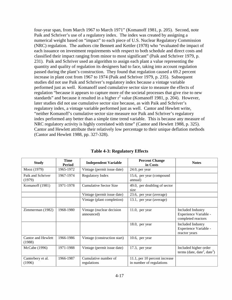
4-17

four-year span, from March 1967 to March 1971” (Komanoff 1981, p. 205). Second, notePaik and Schriver’s use of a regulatory index. The index was created by assigning anumerical weight based on “impact” to each piece of U.S. Nuclear Regulatory Commission(NRC) regulation. The authors cite Bennett and Kettler (1978) who “evaluated the impact ofeach issuance on investment requirements with respect to both schedule and direct costs andclassified their impact ranging from minor to most significant” (Paik and Schriver 1979, p.231). Paik and Schriver used an algorithm to assign each plant a value representing thequantity and quality of regulation its designers had to face, taking into account regulationpassed during the plant’s construction. They found that regulation caused a 69.2 percentincrease in plant cost from 1967 to 1974 (Paik and Schriver 1979, p. 235). Subsequentstudies did not use Paik and Schriver’s regulatory index because a vintage variableperformed just as well. Komanoff used cumulative sector size to measure the effects ofregulation “because it appears to capture more of the societal processes that give rise to newstandards” and because it resulted in a higher r2 value (Komanoff 1981, p. 204). However,later studies did not use cumulative sector size because, as with Paik and Schriver’sregulatory index, a vintage variable performed just as well. Cantor and Hewlett write,“neither Komanoff’s cumulative sector size measure nor Paik and Schriver’s regulatoryindex performed any better than a simple time trend variable. This is because any measure ofNRC regulatory activity is highly correlated with time” (Cantor and Hewlett 1988, p. 325).Cantor and Hewlett attribute their relatively low percentage to their unique deflation methods(Cantor and Hewlett 1988, pp. 327-328).

Table 4-3: Regulatory Effects

StudyTime

Period Independent VariablePercent Change

in Costs Notes

Mooz (1979) 1965-1972 Vintage (permit issue date) 24.0, per year

Paik and Schriver(1979)

1967-1974 Regulatory Index 15.6, per year (compoundannual)

Komanoff (1981) 1971-1978 Cumulative Sector Size 49.0, per doubling of sectorsize

Vintage (permit issue date) 23.6, per year (average) Vintage (plant completion) 13.1, per year (average)

Zimmerman (1982) 1968-1980 Vintage (nuclear decisionannounced)

11.0, per year Included IndustryExperience Variable -completed reactors

18.0, per year Included IndustryExperience Variable -reactor years

Cantor and Hewlett(1988)

1966-1986 Vintage (construction start) 10.6, per year

McCabe (1996) 1971-1988 Vintage (permit issue date) 17.3, per year Included higher orderterms (date, date2, date3)

Canterbery et al.(1996)

1966-1987 Cumulative number ofregulations

11.1, per 10 percent increasein number of regulations

4-18

McCabe included higher order terms; the 17.3 percent figure is a linearapproximation of the curve he found. The curve, however, showed cost increases fromregulation leveling off for plants with permits issued in the early 1980s. Canterbery et al.(1996) use the cumulative number of regulations in force at the time of a plant’s constructionas their indicator of regulatory presence, and they find a strong effect, an 11 percent increasein overnight cost for each 10 percent increase in the number of regulations.

In sum, increasing regulation resulted in about a 15 percent yearly increase in plantcosts during the 1970s and 1980s. As many of the studies warn, these percentage-increasenumbers should not be used to extrapolate future effects of regulation. The percentagesprobably capture the effects of some factors other than regulation; for example, costs per kWmay have increased because the industry tried to build large plants before the technology wasmature enough. Moreover, the yearly-increase figures represent regulatory effects from1970s and 1980s regulation, when the industry was young; future regulation may be lessunpredictable. A plausible, but unproven, implication from the results detailed above is thata stable regulatory environment will lead to more constant costs. As Cantor and Hewlettnote: “These results are extremely important since they may be taken by the nuclear industryto imply that a stable regulatory environment… will stabilize costs” (Cantor and Hewlett1988, p. 316).

4.7.2. In-House Management

The difference in costs between projects managed by construction firms and projectsmanaged in-house by the utilities themselves have already been noted. Zimmerman’s rent-capturing hypothesis has been noted: learning rates may be biased downward becauseconstruction firms charge prices significantly above costs. To test his hypothesis,Zimmerman looks at in-house effects and finds that in-house construction projects were,indeed, less costly than projects managed by construction firms. Zimmerman suggests thatin-house savings could be a result of either rent-capturing by construction firms or efficientmanagement by utilities. With his principal-agent approach, McCabe finds that utilities thatmanaged construction in-house exhibited greater learning effects than construction firms. Heattributes the difference to incentives: working under cost-plus contracts and in a cost-uncertain environment, construction firms had no incentive to reduce costs. Although thecause remains unclear, there is general agreement that in-house construction managementresults in lower-cost plants than construction-firm management.

The first two studies, Mooz (1979) and Paik and Schriver (1979), do not include aregression variable for in-house construction. Komanoff performs a separate regression totest for in-house effects, and finds that in-house managed projects were, on average,30 percent more expensive (Komanoff 1981, p. 200). Zimmerman (1982) and Cantor andHewlett (1988) find the opposite: in-house construction yielded 22 percent and 44.3 percentlower costs, respectively (Zimmerman 1982, p. 303; Cantor and Hewlett 1988, p. 327). Asdescribed in Section 4.5.2, McCabe finds that utilities that managed construction themselvesrealized over five times the learning effects of construction firms.

4-19

Cantor and Hewlett point out: “It should be recognized that the use of a binaryvariable to measure the cost differences between the two types of management regimes isdone by necessity. In fact, there may be a range of utility involvement in the constructionmanagement, suggesting that a continuous variable, if one could be derived, would be apreferable measure” (Cantor and Hewlett 1988, p. 329).

In summary, in-house construction management yields lower costs and greaterlearning rates. The cause may be rent-capturing or greater incentives to reduce costs.

4.7.3. Multiple-Unit Sites

Most of the studies include a variable in their regressions to control for first-unitstatus. As noted, utilities often allot a disproportionate fraction of total costs at multi-unitsites to the first unit. By including a variable for first-unit status, the studies ensure that thisdisproportionate allocation does not bias their results. However, the coefficient associatedwith first-unit status tells nothing about whether reactors at multi-unit sites cost more or lessthan stand-alone reactors, but indicates only that the first unit costs more than subsequentunits at a multi-unit site. Only Komanoff seeks to determine whether reactors at multi-unitsites cost less than stand-alones. To control for first-unit bias, Komanoff averages total costsfor a multi-unit site over all the reactors at the site, so that all the reactors at a multi-unit siteare assigned the same cost. He then includes a dummy variable in his regression for multi-unit status, and finds that “multiple units averaged 9.7 percent lower costs than otherreactors” (Komanoff 1981, p. 201).

4.7.4. Economies of Scale and Construction-Time Effects

Because the standard approach studies use overnight costs as the dependent variable,identifying economies of scale correctly is a three-step process. The first step is to calculatewhat effects, if any, scaling up plant size has on overnight costs, “the quantities of land, laborand materials needed to construct a nuclear power plant” (Cantor and Hewlett 1988, p. 318).However, overnight costs, by definition, do not take into account time-related costs likeinterest and inflation. The second step is to determine how scaling-up plant size affectsconstruction time, and the third step is to determine how an increase in construction timeaffects costs. Construction time affects real costs in two ways: an increase in constructiontime results in greater interest and inflation as well as greater overnight costs. Although therelationship between construction time and overnight costs is not immediately clear, Cantorand Hewlett’s evidence of such a relationship is described below. Table 4-4 lists the studies’estimated scale effects. As a reference point, Komanoff wrote in 1981 that “capital costprojections of the U.S. Atomic Energy Commission (AEC), its successor agencies, and thepower industry assume that nuclear costs per kW decline by 20 to 30 percent when reactorsize is doubled” (Komanoff 1981, p. 200).

4-20

Table 4-4: Economies of Scale

StudyScale Economies; Results of

Doubling Unit Size

Scale Economies withIDC/Construction-

Time EffectsMooz (1979) InsignificantPaik and Schriver (1979) N/A; did not use cost per kW as

dependent variableKomanoff (1981) 13 percent reduction in

cost per kWWith IDC effects, 10percent cost reduction

Zimmerman (1982) 11.1 percent reductionIn cost per kW

Cantor and Hewlett (1988) 36.2 percent reduction in costper kW

With constructiontime- overnight costrelationship, 9 percentincrease

McCabe (1996) InsignificantCanterbery et al. (1996) 51 percent reduction in cost per

kW

In Mooz’s study, the size coefficient in his regression was insignificant, implying noeconomies of scale. However, he did not take construction-time effects into account; doingso may have added costs and implied diseconomies of scale. Paik and Schriver (1979) usedplant costs, not costs per kW costs, as the dependent variable, making testing for economiesof scale impossible. Komanoff found that doubling reactor size led to a 13 percent reductionin costs per kW when overnight costs were used as the dependent variable. Komanoffrecognized that construction-time effects had to be considered: “Doubling reactor sizeextended construction time by an average of 28 percent… the resulting increase in IDC addsapproximately 3 percent to real costs, so that the net effect of doubled size is only a10 percent cost reduction” (Komanoff 1981, p. 200). Komanoff’s results imply slighteconomies of scale; however, Cantor and Hewlett’s results (below) indicate that Komanoffshould have considered the construction time-overnight cost relationship in addition to theconstruction time-interest relationship. Zimmerman found that doubling unit size resulted inan 11.1 percent reduction in costs per kW, but the size coefficient had “relatively largestandard error” (Zimmerman 1982, p. 302). Moreover, Zimmerman did not takeconstruction-time effects into account.

Cantor and Hewlett’s study departs from previous studies by accounting for therelationship between construction time and overnight costs. This relationship is not intuitive:overnight costs, by definition, contain no time-related costs. However, Cantor and Hewletthypothesize that construction time might increase overnight costs in three ways.Construction delays could result in morale problems, a stricter regulatory environment (sinceregulation increases with time), and increased hiring costs (since workers often must be laid

4-21

off and then re-hired). They find overnight costs correlated with construction time beyondthe 95 percent significance level. Using just overnight costs and no construction-timeeffects, Cantor and Hewlett find that a doubling of unit size resulted in a 36 percent decreasein costs per kW. However, when the construction time-overnight cost relationship is takeninto account, the longer construction time necessary to build larger plants makes a doublingin plant size 9 percent more expensive, in costs per kW. “Thus, there appears to be someevidence supporting the claims that the industry has attempted to build units that are too largeto be efficiently managed by the constructors” (Cantor and Hewlett 1988, p. 318). Theconstruction time-overnight cost relationship excludes the construction time-interest costrelationship which affects LCOE.

Marshall and Navarro (1991) deal with the measurement rather than the concept ofovernight costs. They observe that the calculation of overnight costs as the sum ofexpenditures over the construction period must be placed on a correct time basis to satisfy therequirements of capital theory. They point out that overnight costs as commonly calculatedcannot accurately represent economies of scale because they leave out construction-timeeffects. The summation of construction expenditures must be dated to the completion date ofthe plant, which requires the proper correction for price-level change in the calculation ofovernight costs. In their test for economies of scale in Japanese nuclear plants usingovernight costs dated to plant completion dates, they find that when overnight costs are usedas the dependent variable, economies of scale seem to exist, but when opening-date overnightcosts are used, the size coefficient is insignificant, implying no economies of scale exist(Marshall and Navarro 1991, p. 153). Although Marshall and Navarro are critical of theprevious studies’ calculation of overnight costs, they come to the same conclusion – ifeconomies of scale exist, they are minimal. McCabe (1996) uses Marshall and Navarro’sopening-date cost and finds the size coefficient insignificant (McCabe 1996, p. 370).Canterbery et al. (1996, p. 558, n. 4) note that Marshall and Navarro’s contention that thedefinition of overnight costs exclude inflation is incorrect.

The results on size effects are diverse. In Mooz’s regression, the size coefficient isinsignificant. Paik and Schriver do not use costs per kW, so their results cannot be used totest for economies of scale. Komanoff finds evidence of slight economies of scale, takinginto account construction time-interest effects but not construction time-overnight costeffects. Cantor and Hewlett find evidence of slight diseconomies of scale, taking intoaccount construction time-overnight cost effects, but not construction time interest effects.Zimmerman finds evidence of modest economies of scale, but the coefficient is onlymarginally significant. Using opening-date overnight costs, both Marshall and Navarro(1991) and McCabe (1996) find no evidence of economies of scale, but Canterbery et al.(1996) find a strong size effect reducing cost. It seems reasonable to conclude that few if anyscale economies existed in nuclear plant construction in the 1970s and 1980s to confound theidentification of learning effects.

4-22

4.7.5. Region

All of the studies included some measure to control for region. Utilities building indifferent regions face different input costs and different inflation rates. Komanoff, Cantorand Hewlett, and McCabe used the Handy-Whitman index to control for regional differencesin cost of living. Other studies do not mention such adjustments. All of the studies include avariable in their regressions to account for different input prices. Studies often noteconstruction labor as a major input that varies significantly in cost across regions.Construction wage rates “are generally about 5 percent higher in the Northeast than in theMidwest and 25 percent higher than in the Southeast” (Komanoff 1981, p. 199). Anotherpotential source of regional cost differences is difficulty finding a site. For example, in thePacific region, builders have had to consider seismic potential, while developers in thedensely-populated Northeast have had to find a site sufficiently far from urban centers.

Table 4-5 shows the results of the studies. The first four (Mooz throughZimmerman), use regional dummy variables. These four studies found that plants built in theNortheast cost more than plants built elsewhere. Komanoff, for example, found that plantsbuilt in the Northeast were “28 percent more expensive, on average, than plants in otherregions” (Komanoff 1981, p. 199). The last two studies, Cantor and Hewlett’s andMcCabe’s, do not use regional dummies, but their regressions confirm that differences inconstruction labor costs account for a good deal of cost differences. Both Cantor andHewlett and McCabe found that regional wage rate correlated with plant cost at 95 percentsignificance (Cantor and Hewlett 1988, p. 326; McCabe 1996, p. 371). Altogether, plantsbuilt in the Northeast were more expensive than plants built elsewhere, to a large extent aresult of construction wage rates.

4-23

Table 4-5: Regional Cost Differences

Study

Numberof RegionsControlled

For

IndependentVariable Findings

Mooz (1979) 5 Dummy Northeast 38.8 percent moreexpensive than other regions

Paik andSchriver (1979)

4 Dummy South 21.3 percent cheaper, Mountain 23percent cheaper than Northeast and Central

Komanoff(1981)

3 Dummy Northeast 28 percent moreexpensive than other regions

Zimmerman(1982)

5 Dummy Midwest 28.1 percent, South 30.2 percent,Mountain/Texas 39.3 percent, Pacific 14.8percent less expensive than Northeast

Cantor andHewlett (1988)

50 Constructionlabor wage ratein state whereplant is located

Labor wage rate by state correlated withplant costs per kW at 95 percentsignificance

McCabe (1996) 4 Average unionwage rate inBLS region

Average wage rate by region correlated withcosts per kW plant at 95 percentsignificance

4.8. Forgetting and Knowledge Depreciation

Organizational forgetting (or alternatively, knowledge depreciation) occurs whenknowledge is lost during a break in production. Argote and Epple (1990) note: “Knowledgecould depreciate because individual employees forget how to perform their tasks or becauseindividuals leave the organization and are replaced by others with less experience” (Argoteand Epple 1990, p. 922). The concept of organizational forgetting is relevant to the presentstudy because of both the long-term hiatus in nuclear construction in the United States andthe potential for short-term interruptions should construction resume.

Argote and Epple summarize the literature on knowledge depreciation inmanufacturing; none specific to construction was found. They cite one study in which unitcosts were higher after a break such as a strike, and another study that found “recent outputrates may be a more important predictor of current production than cumulative output”(Argote and Epple 1990, p. 921). Argote and Epple also cite Lockheed’s experience with theL-1011 Tri-Star as an example of knowledge depreciation: after a period of low productionof the Tri-Star, Lockheed’s costs were higher than when production first began.

Knowledge depreciation is relevant to near-term nuclear construction in the UnitedStates in so far as recent experience from overseas plant construction is not perfectly

4-24

transferable. If the overseas experience were not transferable at all, the only experience theU.S. industry possesses would be from 1970s-1980s era construction. No literature wasfound on international transfer of construction learning. Knowledge depreciation also shouldbe considered when projecting future learning rates: if construction is sporadic, learningeffects will suffer.

4.9. Conclusion

The evidence from international nuclear construction implies that standardizationincreases learning effects. The evidence from U.S. nuclear construction history, especiallywhen compared with overseas construction, implies that unpredictable regulation reducespotential for learning. Moreover, the literature on knowledge deprecation implies thatconstruction stoppages impair learning by doing. The extent to which the U.S. nuclearconstruction industry is competitive is especially important: the significant differencebetween in-house and agent-managed learning rates implies that incentives to reduce costs(as from competition) are a catalyst for learning by doing to exist—or at least affect wherethe savings go.

Based on the literature with its mixed results and the considerations of Chapter 3, areasonable range for future learning rates in the United States nuclear industry is 3 to 10percent. The upper part of this range is reasonable if nuclear plants are standardized, if theregulatory environment is stable, if the nuclear plant construction industry is competitive, andif engineering teams and construction crews are kept more or less continuously employed.The lower part of the range is more reasonable if the number of units that can be built at asingle site is limited, and construction across sites is discontinuous.

In light of the empirical evidence, a conservative learning rate is 3 percent. It isappropriate for a scenario in which regional demand for new capacity is sufficiently saturatedthat only a single new 1,000 MW reactor could be built at a facility. Orders are spaced apartby a year or more, allowing engineering teams and construction crews to be reassigned.Orders are allocated among several types of reactor, spreading experience across differenttechnologies. Some construction delays allow dispersal of personnel. The structure of theconstruction market lets construction firms retain a large proportion of cost savings fromlearning as profits rather than passing them on to the buyers.

A medium learning rate is 5 percent. It is appropriate for a scenario featuring more orless continuous construction, but not necessarily many cases of sequential units built at asingle facility. A narrower array of reactor designs would be built, and competition in theconstruction industry would cause more of the cost reductions from learning to be passed onto buyers. Construction delays would be uncommon.

An aggressive learning rate would be 10 percent. A continuous stream of orderswould keep engineering teams and construction crews together and there would be moreinstances of building multiple reactors at the same site. Several reactor designs might be

4-25

deployed, but each in sufficient numbers to obtain maximal learning among all parties, frommanufacturing through engineering and construction. Regulation would streamlineconstruction times, and delays would be largely eliminated.

Table 4-6 summarizes the conditions associated with different learning rates.

Table 4-6: Conditions Associated With Alternative Learning Rates

LearningRate

(Percent forDoubling

Plants Built)

Pace ofReactorOrders

Number ofReactors Builtat a Single Site

ConstructionMarket

Reactor DesignStandardization

RegulationImpacts

3 Spread apart1 year ormore

Capacitysaturated, nomultiple units

Not highlycompetitive; canretain savings fromlearning

Not highlystandardized

Someconstructiondelays

5 Somewhatmorecontinuousconstruction

Somewhatgreater demandfor new capacity;multiple unitsstill uncommon

More competitive;most cost reductionsfrom learning passedon to buyers

Narrower array ofdesigns

Delaysuncommon

10 Continuousconstruction

High capacitydemand growth;multiple unitscommon

Highly competitive;all cost reductionspassed on

Several designs;sufficient orders foreach to achievestandardizationlearning effects

Constructiontime reducedand delayslargelyeliminated

4-26

References

Argote, Linda, and Dennis Epple. (1990) “Learning Curves in Manufacturing,” Science 247:920-924.

Argote, Linda, Sara L. Beckman, and Dennis Epple. (1990) “The Persistence and Transfer ofLearning in Industrial Settings,” Management Science 36: 140-153.

Canterbery, E. Ray, Ben Johnson, and Don Reading. (1996) “Cost Savings from NuclearRegulatory Reform: An Econometric Model,” Southern Economic Journal 62: 554-566.

Cantor, Robin, and James Hewlett. (1988) “The Economics of Nuclear Power: FurtherEvidence on Learning, Economies of Scale, and Regulatory Effects,” Resources and Energy10: 315-335.

David, Paul A., and Geoffrey S. Rothwell. (1996) “Standardization, diversity and learning:Strategies for the coevolution of technology and industrial capacity,” International Journal ofIndustrial Organization 14: 181-201.

Epple, Dennis, Linda Argote, and Rukmini Devadas. (1991) “Organizational LearningCurves: A Method for Investigating Intra-Plant Transfer of Knowledge Acquired throughLearning by Doing,” Organization Science 2: 58-73.

Hatch, Nile W., and David C. Mowery. (1998) “Process Innovation and Learning by Doingin Semiconductor Manufacturing,” Management Science 44: 1461-1477.

Irwin, Douglas A., and Peter J. Klenow. (1994) “Learning-by-Doing Spillovers in theSemiconductor Industry,” Journal of Political Economy 102: 1200-1227.

Komanoff, Charles. (1981) Power Plant Cost Escalation. New York: Komanoff EnergyAssociates.

Lester, Richard K., and Mark J. McCabe. (1993). “The Effect of Industrial Structure onLearning by Doing in Nuclear Power Plant Operation,” The RAND Journal of Economics 24:418-438.

Joskow, Paul L., and Nancy L. Rose. (1985). “The Effects of Technological Change,Experience, and Environmental Regulation on the Construction Cost of Coal-BurningGenerating Units,” RAND Journal of Economics 16: 1-27.

Kouvaritakis, Nikolaos, Antonio Soria, and Stéphane Isoard. (2000) “Modeling EnergyTechnology Dynamics: Methodology for Adaptive Expectations Models with Learning byDoing and Learning by Searching,” International Journal of Global Energy Issues 14: 104-115.

4-27

MacLachlan, Ann. (1984) “Key to Cheaper French Nuclear Plants is Labor Use, StudyShows,” Nucleonics Week 25: 9-10.

McDonald, Alan, and Leo Schrattenholzer. (2001). “Learning rates for energy technologies,”Energy Policy 29: 255-261.

Marshall, John M., and Peter Navarro. (1991) “Costs of Nuclear Power Plant Construction:Theory and New Evidence,” RAND Journal of Economics 22: 148-154.

McCabe, Mark J. (1996) “Principals, Agents, and the Learning Curve: The Case of Steam-Electric Power Plant Design and Construction,” The Journal of Industrial Economics 44:357-375.

Mooz, William E. (1979) A Second Cost Analysis of Light Water Reactor Power Plants.Santa Monica: The Rand Corporation, R-2504-RC.

Navarro, Peter. (1988) “Comparative Energy Policy: The Economics of Nuclear Power inJapan and the United States,” The Energy Journal 9, No. 4: 1-15.

Paik, Soon, and William R. Schriver. (1979) “The Effect of Increased Regulation on CapitalCosts and Manual Labor Requirements of Nuclear Power Plants,” The EngineeringEconomist 26: 223-244.

Thomas, S.D. (1988). The Realities of Nuclear Power: International Economic andRegulatory Experience. New York: Cambridge University Press.

Wright, T.P. (1936). “Factors Affecting the Cost of Airplanes,” Journal of AeronauticalScience 3: 122-128.

Yelle, Louis E. (1979). “The Learning Curve: Historical Review and ComprehensiveSurvey,” Decision Sciences 10: 302-328.

Zimmerman, Martin B. (1982) “Learning Effects and the Commercialization of New EnergyTechnologies: The Case of Nuclear Power,” Bell Journal of Economics 13: 297-310.

4-28

5-1

Chapter 5. FINANCING ISSUES

Summary

As a prelude to considering energy scenarios for the future, which will be thecapstone of the study in Chapters 9 and 10, this chapter develops the basic financial modelused to analyze nuclear energy economic viability. Features of the U.S. tax system areintroduced. Risk is considered in some depth. To provide a benchmark for the energyscenarios for the future that will contemplate alternative nuclear energy policies, the model isused to estimate the sensitivity of economic viability to uncertainties in the no-policy case.

Taxes

Recognition that nuclear energy plants will be owned and operated by utilities orother private providers requires introducing tax treatment of debt and equity, deduction ofdepreciation from taxable income with effects of different allowed depreciation schedules,effects of special tax provisions, and effects of inflation on taxes.

Risk

The perceived risk of investments in new nuclear facilities is widely appreciated tocontribute to the risk premium on any new nuclear construction. Principal sources of risk arethe possibilities that new plants will exceed original cost estimates and that constructiondelays will escalate costs. In this chapter guidelines from the corporate finance literature areused to specify likely relationships between project risk and risk premiums for corporatebonds and equity capital. Risk premiums have an important influence on the economiccompetitiveness of nuclear energy. A 3 percent risk premium is used for the first few plants.

No-Policy Scenarios

In using the financial model to study sensitivity to uncertainties, an overnight costrange for new nuclear plants of $1,200 to $1,800 per kW is used, based partly on the threetechnologies discussed as being realistic in Chapter 3. Given the capital cost range, theLCOE of new nuclear plants in the absence of policies is from $53 to $71 per MWh, with a7-year construction time. The range is lower at $47 to $62 per MWh with a 5-yearconstruction time. Costs remain outside the range of competitiveness with coal and gas,which have LCOEs of $33 to $41 per MWh and $35 to $45 per MWh, respectively.

The nuclear LCOE for the most favorable case, $47 per MWh, is close but still abovethe highest coal cost of $41 per MWh and gas cost of $45 per MWh. Longer debt terms andlonger plant life span reduce nuclear LCOEs, but still do not bring them into the competitiverange. The impact of construction delays is large, particularly if a 2-year delay occurs afterall outlays have been made—capable of making the nuclear LCOE range from $61 to over$76 per MWh. These no-policy results provide benchmarks indicating the extent to whichpolicies to be considered in Chapters 9 and 10 are needed to reduce nuclear LCOEs.

5-2

Outline

5.1 Introduction

5.2. The Financial LCOE Model

5.2.1. Basic Equation5.2.2. Capital Investment5.2.3. Interest5.2.4. Taxes5.2.5. Depreciation

5.3. Theory and Evidence on Risk Premiums and Capital Structure

5.3.1. The Nature of Financial Risks Facing New Nuclear Plants5.3.2. Previous Studies of the Decision to Build Nuclear Plants5.3.3. Required Rates of Return on Equity5.3.4. Required Rates of Returns on Corporate Bonds5.3.5. Debt-to-Equity Ratios5.3.6. Debt Maturity5.3.7. Conclusions on Financial Effects of New Nuclear Plant Risk

5.4. No-Policy Scenario Analyses of LCOEs

5.4.1 Nuclear versus Fossil Plants: Economic Advantages and Disadvantages5.4.2. Parameter Values Used for the No-Policy Case5.4.3. Competitiveness of Nuclear Power in the No-Policy Case5.4.4. Sensitivity Analysis for First Nuclear Plants

5.5. Conclusion

References

5-3

5.1. Introduction

To ascertain the conditions under which nuclear power will be competitive in themarketplace requires a financial model of private sector decisions. The required model ismore elaborate than the LCOE model of Chapter 1 used to compare LCOEs in previousstudies, because of tax considerations omitted there. Within the required financial model,careful attention is paid to rates of return on debt and equity that investors will demand inview of market perceptions of the riskiness of nuclear power investments. Introducing theseconsiderations permits estimation of the cost of electricity that will have to be covered byrevenues of operators of new nuclear facilities if these facilities are to be viewed by theprivate sector as warranted investments. These costs in the no-policy case are the startingpoint for considering policies that would make nuclear power competitive.

Section 5.2 develops the financial model that will be used for policy analysis in thepresent study. Section 5.3 reviews the finance literature for guides to risk premia and capitalstructure to be expected for new nuclear facilities. Section 5.4 lays out baseline assumptionsin the absence of policies aimed at the nuclear power industry and applies the financial modelto arrive at LCOEs in the no-policy case. Sensitivities to the baseline assumptions areexplored.

5.2. The Financial LCOE Model

5.2.1. Basic Equation

The levelized cost of electricity, or LCOE, is defined as the constant real price ofelectricity over the life of the plant that compensates debt and equity investors at theirrequired rates of return. Interest on debt accrues during the construction period and debtholders are repaid with equal annual payments over the debt term. Equity holders investduring the construction period and receive profits after tax and debt payment over the plantlife. The LCOE is the electricity price that yields the internal rate of return required byequity holders on the returns accruing to them.

Equity is considered, with debt as an expense, rather than treating them symmetricallyas in the pre-tax LCOE model, because of the different tax treatment of debt and equityreturns. LCOE is the electricity price that solves the following equation:

PRESENT VALUE OF EQUITY INVESTMENT DURING THE CONSTRUCTION PERIOD

= PRESENT VALUE OF NET REVENUE EARNED BY EQUITY OVER THE LIFE OF THE PLANT

where

NET REVENUE = EARNINGS FROM LCOE REVENUE BEFORE INTEREST AND TAXES (EBIT)

– INTEREST EXPENSE – TAX EXPENSE + DEPRECIATION – REPAYMENT OF DEBT

5-4

Annual gross revenue equals the quantity of electricity generated multiplied by itsprice. Revenue in each year t is calculated as annual electricity production multiplied by thenominal electricity price in year t: Rt = QtLt. Electricity production is calculated as plantcapacity in megawatts (W) times the capacity factor (CF), times the number of hours in theyear: Qt=W • 8760 • CFt. The nominal electricity price (Lt) in year t is the levelized cost ofelectricity (LCOE) in 2003 prices compounded at the rate of inflation from the year of theplant’s opening, at time t = 0: Lt = LCOE(1+ )t, where LCOE is the real price of electricityexpressed in 2003 dollars, and is the annual inflation rate.

The expenses consist of yearly fuel cycle costs described in Appendix A5, plus otheryearly variable and fixed operating and maintenance costs and insurance as described inSection 1.4, plus decommissioning costs. The expenses are assumed to grow at the rate ofinflation.

The spreadsheet model uses the GoalSeek function of Excel to solve the equationiteratively for LCOE.

5.2.2. Capital Investment

Overnight cost is the real dollar capital cost at the beginning of the constructionperiod and is allocated equally to each year of the construction period. To accommodate thefeatures of the tax system in this model, it is necessary to allow for inflation, so the realcapital cost must be converted into nominal dollars over the life of the plant. Accordingly,the nominal outflow in each year of the construction period, recorded as negative revenueprior to the beginning of electricity sales, is:

It = C • (1/n) • (1 + )t,

where C is real overnight cost expressed in 2003 dollars, n is total construction time in years,It is the nominal investment in construction year t, where construction is from t= - n to t = -1.Investment is assumed to occur at the beginning of a calendar year.

5.2.3. Interest

Interest costs are deductible against the corporate income tax. They are affected byrisk considerations, which will be analyzed, and by loan guarantees, which is one of thefinancial policies that will be considered.

5.2.4. Taxes

Corporate income tax payments as well as state and local taxes are subtracted fromrevenues. As discussed more fully below, taxes give rise to depreciation allowances.Moreover, the policies aimed at the nuclear power industry to be considered in this studyoperate through affecting tax expense. These policies include investment tax credits,production tax credits, and accelerated depreciation.

5-5

5.2.5. Depreciation

Depreciation only becomes effective in an LCOE calculation when taxes areconsidered, because it is an allowance in the tax code that permits subtraction of an amountof capital expense from a year’s taxable income. With no taxes, the only requirement is torecover the capital cost over the life of the plant. The life of the plant matters, but the timepath at which the plant is assumed to depreciate is irrelevant.

A percent of the depreciable asset base can be deducted from gross income each year.Depreciation begins as the plant starts to operate. Two schedules are employed in the model,the Modified Accelerated Cost Recovery System (MACRS) and Straight Line, to examinethe impact of different depreciation methods on LCOE. The Modified Accelerated CostRecovery System (MACRS) schedule is a 1986 modification of the Accelerated CostRecovery System (ACRS), which was established by the Economic Recovery Tax Act of1981. Both ACRS and MACRS represent a departure from previous depreciation ruleswhich were closely allied to financial depreciation concepts that attempt to depreciate anasset over its economic lifetime. The federal tax code assigns a 15-year depreciation periodto electric utility plants under MACRS (IRS 2002, p. 93). MACRS allows declining balanceor straight-line depreciation for classes of assets that include power plants. Decliningbalance is used here.

The depreciable asset base is measured in nominal dollars at the time ofdisbursement. Consequently a lengthier construction period, or a delay at the end of aconstruction period, would reduce the depreciable asset base relative to overnight costsbecause inflation has more time to raise other prices. This effect reduces the real value of theallowable deduction from revenues and hence would reduce the value of the depreciationallowance. While inflation has offsetting effects on revenues from electricity sales and pricesof fuels and O&M outlays, the effect on the depreciation is not neutral.

During the construction period, part of the financing comes from debt investors andthe other from equity holders. According to accounting rules, interest on debt outstanding iscapitalized and added to the depreciable asset base, so the total asset base consists of nominaldebt investment, equity investment, and interest expenses during the construction period.The depreciable asset base excludes equity appreciation.

5.3. Theory and Evidence of Risk Premiums and Capital Structure

This section is concerned with risk associated with new nuclear plants. The purposeis to develop guidelines for returns on equity, returns on debt and debt-equity ratios, to beused in the financial modeling of the present study. Section 5.3.1 characterizes the risksfacing investments in new nuclear plants. Section 5.3.2 reviews studies of effects ofuncertainty on decisions to build nuclear plants. Section 5.3.3 deals with required return onequity, 5.3.4 with required returns on debt, and 5.3.5 with debt-equity ratios. Section 5.3.6addresses the choice of debt maturity.

5-6

5.3.1. The Nature of Financial Risks Facing New Nuclear Plants

New plants built in the United States in the next decade will have designs that havenever been built in the United States, which increases the construction risks perceivedespecially on the first few units. Construction overseas of these designs, or closely relatedones, will reduce only a part of the construction risk perceived for U.S. construction.

New nuclear power plants are large because the additional size improves theeconomics of a plant’s thermal properties. The large size of the investment can add to therisk premium, particularly when the effect of the additional capacity coming on line in aparticular market is considered. Some new coal plants are the same size or larger, which willtend to raise their risk premiums, but even the larger coal plants are expected to take only anaverage of 4 years to build. The length of the construction period (5 to 7 years) can furtheradd to perceived financial risk (Lesceour and Penz 1999, p. 13).

The regulatory process was a source of construction delays and cost overruns duringthe 1970s and 1980s. The recent combining of construction and operating licenses into asingle step gives hope that construction delays and uncertainties encountered in the lastgeneration of nuclear plants can be avoided in new construction, but in the absence of actualexperience, there is a perception that nuclear plants are riskier than others, as discussed byScully Capital (2002a, 2002b).

5.3.2. Previous Studies of the Decision to Build Nuclear Plants

The influence of risks on an investor’s willingness to undertake a nuclear powerinvestment depends on the source of the risk as well as the level. Pindyck (1993) uses amodel with two types of uncertainty to calculate critical values of expected capital cost innuclear power plants, that is, costs above which an investor will not undertake a project, or ifthe project has begun, will cancel it. One type of uncertainty is technical uncertainty; theother input is cost uncertainty. Technical uncertainty involves uncertainties in completingthe project. These uncertainties become resolved over the implementation period of theproject—they either show themselves to be innocuous, and the project is completed, or theyprove to be insuperable, and the project is abandoned. These risks are largely diversifiable.The input cost uncertainties are largely or totally outside the control of the investor. Wagerates and costs of materials are determined in larger markets, and in the case of nuclearpower projects, these uncertainties include the possibility of regulatory changes. Input costrisk is partly nondiversifiable, because the input prices will be correlated with overalleconomic activity. The greater is the degree of input cost risk, the lower is the critical valueof the expected capital cost that determines the go/no-go decision. The higher are perceivedtechnical risks, the higher is the expected capital cost that the investor will tolerate.

A simple investment rule, using a risk-free interest rate, gives a critical value ofcapital cost per kW. Converting the 1982 prices from Pindyck’s Table 3 (p. 70) to 2003prices reveals a range on critical capital cost values from a high of $2,448 to a low of $1,649.

5-7

Investment is assumed to go forward as long as expected capital costs do not exceed thesevalues.

Pindyck’s study assumes a price of electricity and, using a risk-free interest rate,determines the threshold price of capital above which an investor would not buy a nuclearpower plant. In contrast, the approach of the present study assumes a required price forcapital, and using a weighted average cost of capital that includes an interest premium,determines the price of electricity.

Sommers (1980), using a logit regression analysis of 113 utilities, found that greateruncertainties about nuclear capital costs and construction times lowered the probability that autility would invest in a nuclear plant rather than a coal plant. Capital cost uncertainty had astronger dampening effect on the likelihood of a utility’s investing in a nuclear plant than didthe relative capital cost of nuclear and coal investments.

While the Sommers study corroborates the importance of risk factors this study hasidentified, it focuses on the probability that an investor would undertake construction of anuclear plant. In contrast, the present study addresses the incentives that would be requiredto induce investors to undertake construction.

5.3.3. Required Rates of Return on Equity

5.3.3.1. Traditional CAPM and Its Irrelevance to the Present Study

The most widely used model of equilibrium equity asset pricing remains the capitalasset pricing model (CAPM) of Sharpe (1964), Lintner (1965) and Black (1972) and Mossin(1966). The central implication of the CAPM is that expected returns for each asset (let thisbe ri for asset i) should bear a linear relationship with the expected returns of the market as awhole. The CAPM equation is ri = rf + βi (rm - rf), where βi is a measure of co-movementof each firm with the market. Expected stock returns are higher for firms with highcorrelations with the market return. Investors demand a premium for holding stocks whichare highly correlated with the market, that is, for holding non-diversifiable or systematic risk.A model very similar to the CAPM is a consumption-based capital asset pricing model(CCAPM). This model suggests that expected asset returns have a linear relationship withoverall marginal utility of consumption as determined by performance of the economy atlarge. Though there have been other theories of equilibrium asset pricing, CAPM andCCAPM are still most prevalently used. CAPM has become a central tool of financialanalysis in the finance industry (see for example Graham and Harvey (2001) who find thatfirms rely heavily upon CAPM techniques).

CAPM and CCAPM do not include an effect of own variance of asset returns, aproperty often considered to be counter-intuitive. The reason for lack of effect of ownvariance is brought out in the Markowitz (1959) portfolio selection model (a building blockof CAPM). Investors can completely rid themselves of any assets’ idiosyncratic risk bydiversifying, through the holding of a market basket containing essentially an infinite number

5-8

of securities. Since total market risk cannot be diversified away, only the correlation ofsecurities returns with the market remain as a determinant of a security’s value.

The evidence of the empirical validity of CAPM is mixed at best. Representativestudies are Black, Jensen, and Scholes (1972), Fama and MacBeth (1973) who found limitedsuccess for CAPM over some years, and Fama and French (1992) who find no evidence at allfor the CAPM. Banz (1981), Chan and Chen (1991), Stattman (1980) and Rosenberg et al.(1985) find that other factors besides CAPM beta help to explain equity returns, contrary tothe central tenant of CAPM. The industry has continued to use the CAPM as a central tool infinancial analysis, probably due to 1) its theoretical attractiveness, 2) its easy applicabilityusing easily accessed data 3) lack of a better alternative and 4) its widespread base ofunderstanding among forty years of MBA graduates.

A fundamental point for the present study is that new nuclear plant risk isidiosyncratic and not market risk. The risks involve events that are specific to a nuclear plantand have no expected correlation with overall market events. Thus, according to strictCAPM theory nuclear plant risk should have no effect on investors' valuation of the firm, andthus no effect on the required rate of return on equity for a firm building a nuclear plant.

5.3.3.2. Idiosyncratic Risk

Notwithstanding CAPM theory, own variance (the variance of a stock's returns) andidiosyncratic risk (the standard deviation of the error term from a regression of firm returnson the market over time) are also sometimes tested used as determinants of expected stockreturns, such as in Douglas (1969). These measures fell out of favor in the face of the rapidacceptance of the CAPM and in light of alternative explanations for why own-varianceeffects may falsely appear to explain asset returns, such as is described by Miller and Scholes(1972) and tested by Fama and MacBeth (1973) and Roll and Ross (1980). However,idiosyncratic measures of risk have recently become a focus of renewed attention.

More recent papers, Tolley and Nielson (1992) and Nielson (1993), have reexaminedthis effect and have found support for own variance, both theoretically and empirically.Using techniques similar to Fama and French (1992), Nielson (1993) finds that own varianceindeed explains some of the cross-variation in expected stock returns. Nielson also supportsthe size and the book to market (B/M) effects discussed above, but finds evidence that thesemay be proxies for the own variance effect. For a further contribution and references to otherrecent studies where own variance affects returns, see Tolley and Nielson (2003).

5.3.3.3. Previous Studies of Nuclear Power Equity Returns

Some papers have addressed the financing of nuclear plants specifically. However,these studies are for facilities built in the 1970s and 1980s in an environment which may notbe similar to plants in the future. Most importantly these studies were done when the plantswere fully operational, after they had been completed. Therefore they have little if anybearing on uncertainty about prospective construction costs for a plant with new technology

5-9

not yet built or for regulatory uncertainty surrounding the decision to build a plant, which arerisks of concern the present study. Farber (1991) studied the effect of adopting nucleartechnology on equity costs of electric utilities prior to the Three Mile Island (TMI) accident.Farber studied the effects on equity returns of thirty-six nuclear power adopters and twenty-five non-nuclear firms. He concluded that adoption of a nuclear plant increases a firm’sCAPM equity beta. In addition, he concluded that the leniency of regulators may moderatethe risk-increasing effect of nuclear power. Brooks and D’Souza (1982), Bowen et al.(1983), and Fraser and Kolari (1983) found that the TMI accident appeared to increase theexpected beta risks of four utilities owning nuclear capacity, although Uselton et al. (1986)subsequently found the effect to be transitory.

Hearth et al. (1990) examine the effect on stock prices of cancellations of nuclearpower plants. The authors found that decisions to cancel nuclear power plants underconstruction appeared to result in significant negative excess stock returns. This loss wasfound to be bigger with the ratio of the sunk costs relative to the utility's market value. Kalraet al. (1993) measure the U.S. stock market reaction to the April 1986 nuclear Chernobylpower plant accident. The authors found that after the Chernobyl event the betas for allpower utilities (conventional, mixed and nuclear) rose.

Fuller et al. (1990) studied the reaction of financing environment of three specialevents: Three Mile Island accident, the Chernobyl catastrophe and the Washington PublicPower Supply System bond default. Based upon the authors’ cross-sectional analysis it wasestimated that a 3 percent increase in the allowed rate of return for nuclear utilities wouldhave been required to offset the discount associated with nuclear power.

Hill and Schneeweis (1983) use stock price data to study the effect on the stockreturns of public utility firms of the TMI nuclear accident. The authors find that impact ofthe Three Mile Island accident on non-nuclear electrical utility firms was less than that onnuclear based utilities. Hewlett (1984) found that investors in nuclear firms required a 1 to 2percent risk premium.

As noted, since these studies refer to utilities that already had nuclear plants, refer to apast regulatory environment, and in some cases rely on estimates of beta no longer acceptedin the literature, they are at best suggestive and in any case give little if any help in choosinga required rate of return applicable to a firm that will build a new nuclear plant in the future.

5.3.4. Required Rates of Returns on Corporate Bonds

The academic literature generally assumes (see Elton et al., 2001) corporate debtcarries the same rate of return as U.S. Treasury Bonds plus a premium. The premium iscomprised of three parts 1) a premium for expected default risk, 2) a state tax premium (asincome from corporate bonds is taxed and Treasuries are not), and 3) a premium forattracting risk-averse investors.

5-10

Theoretical reduced-form models explaining risky bond prices (and thereforeexpected returns) include Duffie and Singleton (1997), Jarrow et al. (1997), Lando (1997),Das and Tufano (1996) and Madan and Unal (1998). Option-based models stemming fromthe Black-Scholes (1973) option pricing formula are found in Merton (1997), Longstaff andSchwartz (1995), Galai and Masulis (1976), and Jones and Rosenfeld (1984).

The academic studies attempting to empirically explain corporate bond rates aresparser than for equities. Elton et al. (2001) find that most of the third part (risk aversionfactor) is responsible for most of the bond premium, and that expected default premium isresponsible for the least. Barrett et al. (1986) find a decrease in utility bond prices as areaction to the 1979 Three Mile Island nuclear power plant accident.

Bond rating firms, most notably Standard and Poor’s and Moody, appear essentiallyto evaluate default probability. Recent corporate bond yields were (from Moody, November2003, twenty-year maturities) 5.54 percent for the AAA rated bond, 5.88 percent for the AAgrade bonds, 6.03 for the A rated bonds and 6.59 percent for the Baa grade bonds. Forcomparison, the yields on twenty-year U.S. Treasury bonds during the same period wereabout 5.1 percent.

Altman and Kishore (1998) find the following percentages of par recovery rates onemonth after firms declare bankruptcy by grades of debt : AAA have about 68 percent ratesof recovery, AA and A have about sixty percent, BBB bonds have about 49 percent, BB39 percent, B and CCC 38 percent, and default have zero percent recovery rates.

5.3.5. Debt-to-Equity Ratios

The finance literature on the determinants of the debt-equity ratio is mixed. Astarting point is the Modigliani and Miller (1958) study showing that under certainassumptions the debt-equity ratio is irrelevant. Current opinion is split between two maincompeting theories, neither of which is completely convincing in light of empirical tests.First, the static trade-off model proposes that firms have a target debt-equity ratio. In thismodel, debt has certain advantages: debt possibly lowers taxes, increases monitoring ofmanagement and motivates management. These advantages are weighed against debt’sdrawbacks, as noted in Jensen and Meckling (1976) and Myers (1977): possibly higherexpected bankruptcy costs and higher costs due to agency problems.

The main competing theory is the Myers (1984) and Myers and Majluf (1984)pecking order theory. Here, asymmetric information and transactions costs drive firms tofinance operations in the following order 1) retained earnings, 2) safe debt, 3) somewhatriskier debt and finally 4) riskier debt and equity. Once again, equity is more expensive dueto asymmetric information: management knows more about firm outcomes than outsidefinanciers who will, sometimes, be induced to buy over-priced equity. That is, equity will beover-priced due to asymmetric information, management knows that current shares are over-priced, reducing debt.

5-11

Much of the empirical work of an academic nature related to debt-equity ratios doesnot focus on risk. Work which does speak to risk generally finds a small role for risk incapital structure. See for example, Marsh (1982), Ghosh et al. (2000), Kale et al. (1991) andFama and French (2003).

There is an on-going debate on whether industry-specific effects on debt-equity ratiosexist. Schwartz and Aronson (1967), Scott (1972), Scott and Martin (1975), Bowen et al.(1982), Martin and Henderson (1984) and Bradley et al. (1984), Hull (1999), and Sibley(1999) find inter-industry differences in debt equity ratios. Remmers et al. (1974), Belkaoui(1975), and Sekely and Collins (1988) all fail to find evidence of differences in debt-equityacross industries. Graham and Harvey (2001) surveyed 392 CFOs regarding their use offinancial tools and targets. The responses indicated that if firms do have leverage targets,those targets are quite soft.

5.3.6. Debt Maturity

Multiple factors influence corporate borrowers’ and lenders’ choice of debtmaturities. Moreover, debt maturity, debt-equity ratio and risk premium are interrelated. Anumber of models relate risk and capital structure to maturity choice, but no comprehensivemodel of all three choices has been found. The first sub-section (5.3.6.1) places maturitychoice within the general context of the term structure of interest rates. The second sub-section (5.3.6.2) addresses informational asymmetry problems that may pose important risksin financing new nuclear power plants. The third sub-section (5.3.6.3) deals with theinfluence of other risks on maturity choice, and the fourth (5.3.6.4) discusses the influencesof transaction costs and taxes. The fifth sub-section (5.3.6.5) addresses interactions betweenchoices of debt maturity and capital structure. The sixth sub-section (5.3.6.6) reviewsempirical evidence on risk and debt maturity. The final sub-section (5.3.6.7) summarizes.

5.3.6.1. Term Structure

The term structure of interest rates underlies debt maturity choices. An importantconsideration is the slope of the term structure, i.e., rate of rise of interest rates that must bepaid as maturity length increases. Empirical evidence has shown that firms take into accountthe relative cost of short- and long-maturity bonds when issuing debt (Barclay and Smith1995, Guedes and Opler 1996, Stohs and Mauer 1996, Graham and Harvey 2001). Otherthings being equal, firms gravitate to shorter maturity instruments when term structure slopesare steep, and toward long term instruments when slopes are shallow or negative. However,the slope of the term structure is clearly not the only determinant of maturity choice as thefollowing sub-sections bring out.

5.3.6.2. Influences of Asymmetric Information on Debt Maturity Choice

When a lender either cannot assess the accuracy of a borrower’s informationregarding a project, or when a lender cannot easily monitor the actions that a borrower agreesto undertake as part of a loan contract, asymmetric information problems exist. One problem

5-12

is signaling. Another is the principal-agent, or agency, problem. Both problems areamenable to sorting solutions. Lenders devise a menu of debt maturities and interest ratesthat would leave them equally well off and let borrowers reveal their private information byselecting a particular combination that best serves their own interests.

In the signaling problem with private information, lenders cannot easily assess theaccuracy of information borrowers provide. This situation occurs for construction costestimates for new nuclear power plants. As the Scully report (2001a) brought out, oneconcern of investors is that vendors’ cost estimates may not be borne out. Modeling of thisproblem suggests that borrowers with prospects that are unobservable to lenders chooseshort-term debt due to bond holders’ fears that the firm may have poor prospects andconsequently would be willing to give low rates only for short term bonds (Flannery 1986;Kale and Noe 1990; Rousseau 1999; Diamond 1991, 1993; Diamond and Rajan 2001; Bergeret al. 2003). Firms with good prospects that are observable only to management sell short-term bonds because management knows that after its prospects are recognized as good bylenders, the firm can then re-finance at lower rates. Barclay and Smith (1995) find evidencethat firms use debt maturity to signal information and firms with larger informationasymmetries issue shorter term debt, and Benmelech (2003) finds evidence that firms withmore salable, or redeployable, assets have longer debt maturities, implying a possiblesignaling with maturity. Antoniou et al. (2002) find no association of debt maturity with firmquality among French and German firms, which they suspect is due to those countries’ legalstructures, and modest support for signaling with maturity among U.K. firms. Bali andSkinner (2003) find evidence that higher project risk leads to shorter maturity.

In a well-known financial agency problem (Jensen and Meckling 1976; Myers 1977),firms that are recognized as having opportunities to transfer wealth from bondholders toequity holders by increasing the riskiness of their operations during the term of the contract,can signal their willingness to forego such opportunities by selling debt at the shorter end ofthe maturity spectrum. In the case of a loan on a nuclear power plant, where agency costscould exist is in ensuring construction quality. As part of the regulatory process, the utilitymust specify the characteristics of the plant in considerable detail. The U.S. NuclearRegulatory Commission (NRC) reviews the plans, and under the revised 10 CFR 52, willissue a combined construction and operating license. Permission to operate is subject toconfirmation that the actual construction conforms to plans. This supervisory function ofNRC serves at least partially to assure the lender that the borrowing utility is performingaccording to contract. From the lender’s perspective, if the construction is not performed inaccordance with the contract, which would be determined by NRC inspections, the borrowerwould incur additional construction costs, possibly jeopardizing the repayment of the loan.A utility could signal its belief that its construction quality will meet NRC’s standards bytaking a shorter maturity loan.

5-13

5.3.6.3. Effects of Non-Informational Risks on Debt Maturity Choice

Liquidity risks tend to push debt maturities to the long end of the spectrum. Atemporary problem could force issuers to refinance at unattractive rates. If bad news about aborrower arrives near the refinancing date, investors would raise the default premium on newdebt. Firms with projects that could experience temporary problems will be motivated tohold longer-term debt, so as to face the debt renewal less frequently (Johnson 1967, Flannery1986, Diamond 1991).

Some firms will want to match maturities of their liabilities and their assets. Thismotivation would be stronger when transactions costs and liquidity risks are higher (Mitchell1991, Sarkar 1999). A bond would mature at the date an asset is to be sold or begingenerating positive cash flow, avoiding both the need to roll over shorter maturity bonds andthe higher cost of longer term bonds. Morris (1976) finds that financing long-lived assetswith short-maturity debt could decrease the uncertainty of net income if interest rates arepositively correlated with net operating income.

5.3.6.4. Transactions Costs and Taxes

Small debt issues have proportionally higher transactions costs than large issues.Large firms, such as those likely to build new nuclear power plants, would tend to chooseshorter term debt to take advantage of lower market rates at the shorter end of the termstructure (Fisher et al. 1989). In general, long-term debt allows its holders greater flexibilityin timing of capital gain and loss declarations, and this flexibility is an option having value.Firms can sell long-term bonds for relatively more than short term bonds if this tax-timingoption is highly valued (Brick and Palmon 1992).

Interest rate volatility reduces the present value of debt tax shields from short-termfinancing, making long-term debt attractive when interest rates are volatile (Guedes andOpler 1996, Brick and Ravid 1985, 1991; Kim et al. 1995). If new nuclear plants reachedfinancing stages during a period of volatile interest rates, borrowers could be expected towant longer debt maturities. Kane et al. (1985) model the tax advantage to debt, net of amarket premium for added bankruptcy risk, adjusting maturity and the debt-equity ratio tomaximize firm value including the tax shield, with the result that optimal maturity isnegatively associated with the tax advantage of debt. As the value of a tax shield falls, thedebt-equity ratio falls and maturity lengthens. Policies that reduced tax obligations on newnuclear plants could increase the value of longer maturities.

5.3.6.5. Interactions between Choices of Debt Maturity and Capital Structure

To the extent that risks are affected by both debt-equity ratios and debt maturity, thetwo choices will be made simultaneously. For example, in a world of agency problems,should the debt-equity ratio be so low that bankruptcy is almost impossible, the incentive tolower debt maturity as a signal would disappear and the firm would move to a longer

5-14

maturity. In this way there is a trade-off between debt-equity ratio and debt maturity (Lee etal. 1983, Diamond 1991, Leland and Toft 1996, Elyasiani et al. 2002, Ju and Ou-Yang 2003).

5.3.6.6. Empirical Evidence on Relationships between Risk and Debt Maturity

Stohs and Mauer (1996) find that larger and less risky firms with longer-term assetmaturities use longer-term debt, debt maturity varies inversely with earnings surprises and afirm’s effective tax rate, and firms with high and very low bond ratings use short-term debt.Guedes and Opler (1996) find that large firms with high credit ratings tend to borrow at veryshort and very long terms, while low rated firms borrow at the middle of the spectrum, whichthey suggest is consistent with a trade-off between liquidity and agency effects.

5.3.6.7. Conclusions on Debt Maturity

Debt maturity is influenced by both project and firm characteristics. The choice ofmaturity involves a trade-off with interest rates and the debt-equity ratio. Informationaluncertainties tend to encourage shorter-term debt. Firms financing assets that are eitherriskier or perceived to be riskier typically find some advantage to borrowing at shortermaturities, other influences being equal. Tax considerations and the correlation of a firm’sincome with economy-wide indicators such as interest rates or a stock market index also caninfluence maturity choice. The debt-equity ratio and maturity tend to move in oppositedirections in the valuation of tax shields. A judgmental conclusion is that the variousinfluences, on net, work against choice of highly lengthy maturities in the financing of newnuclear power plants.

5.3.7. Conclusions on Financial Effects of New Nuclear Plant Risk

Most of the finance literature on equity returns, bond returns and debt-equity ratioshas dealt with a large number of considerations, with risk as such being considered if at all asonly one consideration. The bottom line is that no readily identifiable - much lessempirically verifiable - estimate of the effects of a new nuclear plant on a firm’s finances isavailable from the literature. A strand running through the work reviewed is that withjudicious relaxation of the stringent assumptions of traditional finance theory there could bean effect of own risk. It should be noted that, apart from academic investigation, receivedopinion of practitioners is that these effects exist both for equity and debt returns. Theliterature does, however, suggest relatively shorter debt terms for investments with thecharacteristics of new nuclear plants. The foregoing considerations inform the judgmentalchoices of financial effects of new nuclear plants to be used in the financial modeling of thepresent study.

5.4. No-Policy Scenario Analyses of LCOEs

Section 5.4.1 reviews the characteristics of nuclear and fossil plants that contribute totheir relative economic advantages. Section 5.4.2 reports the values of cost and performance

5-15

and market variables used in the LCOE calculations in the benchmark no-policy case.Sections 5.4.3 and 5.4.4 discuss the use of these variables in sensitivity and scenario analysis.

5.4.1. Nuclear versus Fossil Plants: Economic Advantages and Disadvantages

Nuclear power has several advantageous economic characteristics, but also suffersfrom a number of disadvantageous characteristics as perceived by investors, as summarizedby LaBar (2002). Advantageous economic characteristics are as follows:

• Low and predictable fuel and operation and maintenance (O&M) production costs.Nuclear production costs exhibit low volatility over both the short and long termbecause the primary energy source, uranium ore, represents a very small fraction ofthe total production cost. On the other hand, the cost of the primary energy source infossil-fired plants is a large fraction of the production cost.

• High capacity factors. The operating nuclear plants in the United States nowconsistently achieve fleet-average capacity factors in the 90 percent range. Theprojected lifetime averaged capacity factors for competing baseload gas-firedcombined cycle plants are in the range of 80 to 85 percent.

• Long Operating Lifetime. Operating lifetime licensing extensions have been obtainedfor several U.S. nuclear plants and more are expected in the future. New nuclearplants are being designed for a 60-year life. On the other hand, there is littleexperience in the long-term operation of competing baseload gas-fired combinedcycle plants. Nominal gas-fired combined cycle plant lifetimes are not expected toexceed 25 years.

Disadvantageous economic characteristics of nuclear power are:

• Large plant size. Most new nuclear power plants are designed in the size range of1,000 to 1,350 MW to gain economy of scale benefits and reduce the capital costsper kW. A drawback of this size range is high potential for exceeding demandgrowth. Widely used baseload gas-fired combined cycle plants are in the range of500 to 600 MW.

• Large capital outlay. Total overnight capital costs of new nuclear plants are estimatedto be in the $1,000 to $1,800 per kW cost range. For a 1,350 MW plant at $1,600 perkW, an investment of $2.16 billion can be required, excluding interest costs. Thecompeting baseload gas-fired combined cycle plant capital cost is in the $450 to $650per kW range. A 600 MW combined cycle plant at $650 per kW would require aninvestment of less than $0.4 billion.

• Long construction time. The construction time for new nuclear plants, even ifoptimized to achieve short construction times, is in the range of 3 to 4 years. Theconstruction period for competing gas-fired combined cycle plant is about 2 years.

5-16

• Investment financing. The higher capital cost results in a higher total investment atrisk and the longer construction time results in higher interest costs duringconstruction as well as longer time-at-risk. These factors contribute to requiredreturns on equity and debt.

The investment-financing hurdle may become easier to overcome as nuclear plantownership has become increasingly concentrated. Twelve utilities, plus Tennessee ValleyAuthority (TVA), now own and operate nearly two-thirds of plants. The larger owners, nowwith 75 percent of U.S. capacity, are able to manage a portfolio of units. They can considerfinancing new units based on a larger balance sheet of total asset value. In addition, stockprices of nuclear utilities have recently outperformed non-nuclear utilities (Scully Capital2002). Thirteen utilities account for 75 of the 103 nuclear plants and all of them areoperating more than 2,000 MW of electrical capacity.

5.4.2. Parameter Values Used for the No-Policy Case

Table 5-1 identifies the parameter values used for the important parameters incalculations of LCOEs under the assumption that no policies are employed.

The three capital costs correspond to four nuclear plant designs, each with its ownovernight cost, selected for analysis, as already discussed in Section 3.4. To review, onedesign is a mature plant, the FOAKE costs on which have already been paid. The ABWRand ACR-700 are such designs. Their overnight cost is assigned a value of $1,200 per kW.Another design is a plant that has not yet been built, the FOAKE costs on which are yet to bepaid, such as the AP1000. On the assumption that the entire FOAKE cost is assigned to thefirst plant, this plant’s cost is $1,500 per kW. The third capital cost is chosen to represent theFramatome reactor under consideration for construction in Finland. Its overnight cost is$1,800 per kW.

5-17

Table 5-1: Parameter Values for No-Policy Nuclear LCOE Calculations

Item Parameter ValueOvernight Capital Cost $1,200 per kW $1,500 per kW $1,800 per kWPlant Life 40 yearsConstruction Time 7 yearsPlant Size 1,000 MWCapacity Factor 85 percentHours per Year 8,760 hoursCost of Debt 10 percentCost of Equity 15 percentDebt Term 15 yearsDepreciation Term 15 yearsDepreciation Schedule MACRSa

Debt Finance 50 percentEquity Finance 50 percentTax Rate 38 percentNuclear Fuel Cost $4.35 per MWhNuclear Fixed O&M Cost $60 per kWNuclear Variable O&M Cost $2.10 per MWhNuclear Incremental Capital Expense $210 per kW per yearNuclear Decommissioning Cost $350 millionNuclear Waste Fee $1 per MWh

aModified Accelerated Cost Recovery System

5.4.2.1. Nuclear Construction Time

Nuclear construction projects are divided into several phases (DOE 2001a, pp. 13-16;DOE 2001b, pp.4-11 to 4-12). The start-up phase consists of early site permitting, designcertification, plant licensing, site preparation, and procurement of long lead-time componentssuch as pressure vessels and steam generators. Procurement continues during theconstruction phase. The final phase is start-up and testing. The stated DOE position of a5-year construction schedule is based on the new streamlined regulatory policy. The basecase in the present study is 7 years for anticipated construction time. This is the time periodof major financial outlays prior to revenue generation from power sales. The businesssignificance of this period is that it is a time of negative cash flow, during which interestcosts accrue on expenditures. This duration is based on the assumption that the businesscommunity will form expectations taking account not only of the newer announcedregulatory procedures but also of earlier experiences with construction times. The Scullyinterviews with financial and utility executives (Scully 2002a, p. 1-76), as well as anecdotalreports, reinforce the importance to the business community of expectations regardingconstruction time. Deutsche Bank’s LCOE calculations for new nuclear power in the UnitedStates rely on a 7-year construction period (Smith and Hove 2003, Figure 66, p. 77).

5-18

Later policy scenarios in this study allow for revision of expectations from 7-year to5-year construction times for later plants, based on more favorable than expected businessoutcomes with the first few plants. For simplicity, expenditures are assumed to occur equallyin each year of construction. Experiments with more refined patterns of expenditures werefound to be of little consequence.

It is important to recognize that the construction times used in the LCOE calculationsare expected construction times, from which actual construction times may deviate. Theprofitability calculations that inform investment decisions are based on expected values ofthe variables in the LCOE formulation: sale prices of electricity, overnight cost, nuclear fuelcosts, and O&M costs, as well as construction times. The influence of the expectation of theconstruction time on calculated LCOE is particularly important and has been of particularconcern to the investment community. As noted above, the expectation of construction timefor first plants will be heavily influenced by previous U.S. experience. However, newexperience will give investors new data with which to update their expectations, and ifconstruction times turn out to be the 5 years that DOE and vendors emphasize, investors willadjust their expectations accordingly.

5.4.2.2. Base Cost of Capital

The base cost of debt and equity to utilities was assessed from current Bloomberg’sdata (Bloomberg, Inc., 2004), adjusting for maturity and the currently abnormally lowinterest rates. The constituent firms of the Standard and Poor’s 500 Utilities Index were usedas the benchmark for the cost-of-debt and -equity calculations here because those data arewidely used in gauging utility company performances. Individual data on weighted averagecosts (WAC) of debt and equity were taken for 37 of the largest utilities in the United States.Since Bloomberg reports the weighted average cost of debt post-tax, those numbers wereconverted to pre-tax with the formula WAC of Debt Before Tax = WAC of Debt After Tax /(1 – Effective Tax Rate). The effective tax rate for each utility is available from Bloomberg.The average WAC of debt for these utilities, adjusted to pre-tax basis, is 5.34 percent, andthat for equity is 8.63 percent.

In its calculations of the costs of debt and equity for individual utilities, Bloomberguses the 10-year U.S. Treasury bond as the risk-free rate, and adds its own debt and equityrisk factors above that base rate. The 10-year generic government bond traded at 3.747percent on the morning of March 15, 2004. The 30-year government bond traded at a spreadof 1 percent above the 10-year rate, and the 15-year bond traded at 51 basis points above the10-year bond. Thus, adjusting the Bloomberg capital cost estimates for a more appropriatematurity would add between .5 and 1 percentage point to the WACs of debt and equityreported in the previous paragraph.

The current bond yield is at a decadal low, as the Federal Reserve still holds theFederal Funds rate at 1 percent. These low rates are not expected to last long. It would bemore appropriate to use an average of historical rates to smooth out the current aberration.

5-19

Using a 300-day moving average to smooth out the fluctuations in the yield on the generic30-year government gives a return about 50 basis points above the current yield.

Thus the total adjustment to the base rates reported in Bloomberg, to account forterm-structure and the currently low rates, is between 1 and 1.5 percentage points. Theseadjustments give a cost of equity between 9.64 and 10.13 percent and a cost of debt between6.35 and 6.84 percent. For purposes of the present study, these capital cost estimates arerounded to 10 percent for equity and 7 percent for debt.

5.4.2.3. Risk Premium

While the finance literature has much to say about risk and bond and equity rates, itdoes not provide clear, quantitative guidance on the relationship between risk and interestrates, as the above review brings out. Many factors influence the relationship, and thesubject is actively researched. Financial terms in recent nuclear construction overseas are nota satisfactory guide to a risk premium in the United States because of differences amongcountries in business practices, differences in business climate, varying degrees ofinvolvement of governments in nuclear projects, and differences in regulatory regimes.

Themes in the above review are that nuclear plant risk is idiosyncratic (plant specific)rather than beta (market related) and that agreement is lacking on the effect of idiosyncraticrisk on required returns. These considerations hinder estimation of the effect idiosyncraticrisk as a variance concept. However, another and quite direct effect of nuclear plant risk isits effect on expected return. While risk leading to dispersion in possible future returns addsto variance, it also affects the expected returns if it is asymmetrical, as it is in the case of newnuclear plants. For the outcome where all goes according to plan, a normal projection ofreturns can be made. But the upside risk of favorable surprises is less than the downside riskfrom unforeseen delays and the like.

The investor maximizing expected returns will be indifferent between a security withnormal market risk yielding a return of r and an investment with noticeable asymmetricdownside risk yielding some higher return rR, is needed to induce investors to hold the riskiersecurity. The expected gross return for a security with normal market risk is 1+r, whichprovides for paying back the original dollar invested. Through security pricing, investorswill make 1+r equal to the expected return on a security with asymmetric downside risk. Theexpected gross return on the security with asymmetric downside risk is the gross return on adollar invested 1+rR times the probability that the investment will be successful, plus theprobability that it will be unsuccessful times the fraction of the dollar that will be recovered ifunsuccessful, or [pS + (1 - pS)fL](1 + rR) where pS is the probability of a normal or successfuloutcome and fL is the fraction of the dollar that will be recovered in the event of anunsuccessful outcome. Setting 1+r equal to [pS + (1 - pS)fL](1 + rR) and re-arranging gives

1+rR = (1+r)/ [pS + (1-pS)fL].

5-20

Letting the risk premium be , so that rR = r + and solving for gives

= (1 + r){-1 + 1/[pS + (1 - pS)fL]}

which in the special case where nothing is recovered (fL = 0), gives = (1+r)[(1-pS)/pS].

Table 5-2 below shows risk premiums for different combinations of probabilities ofexperiencing an unsuccessful outcome and extent of loss in the event of such an outcome.Each scenario uses a normal rate of return of 10 percent.

Table 5-2: Risk Premiums for Alternative Investment Losses andLoss Probabilities, 1-ps

Percent of Investment Value Recovered (fL):Probability ofUnsuccessful

Outcome (1-pS) 50 25 0 -25 -501.00% 0.6% 0.8% 1.1% 1.4% 1.7%

2.00% 1.1% 1.7% 2.2% 2.8% 3.4%

2.50% 1.4% 2.1% 2.8% 3.5% 4.3%

3.00% 1.7% 2.5% 3.4% 4.3% 5.2%

3.50% 2.0% 3.0% 4.0% 5.0% 6.1%

4.00% 2.2% 3.4% 4.6% 5.8% 7.0%

5.00% 2.8% 4.3% 5.8% 7.3% 8.9%

6.00% 3.4% 5.2% 7.0% 8.9% 10.9%

Loss of 50 percent of the value of the investment, in the first column of Table 5-2,would represent a case in which the investor considers it plausible that construction delays orhigher-than-expected component costs could cause the new plant’s LCOE to be considerablyhigher than the best case. Overruns of this magnitude can occur if cost overruns involvecapital costs, which are the most important component of nuclear power costs, or if delaysoccur that increase the carrying or interest cost before plants begin operation, which again isan important cost component. A loss in asset value would be incurred. The cost overrunscould cause the borrower to default on the loan, leaving the lender to sell the plant for a priceconsistent with an LCOE of competing coal or baseload gas plants which could be half thatof the nuclear plant. A similar scenario could account for column 2, in which 25 cents on thedollar are obtained. The 100 percent loss in column 3 (0 cents on the dollar) would beassociated with the prospect of not being allowed to open the plant after it is built, despite thestructure of the new regulatory system. In columns 4 and 5, the lender also considers theprospect of getting its bond rating downgraded, in addition to its losses on the project. Theproject losses in these cases would decrease the asset value of the firm more extensively thanthrough loss of the direct investment. Each of the alternatives is a set of possible outcomesexpected to occur with probability less than one, a set of possible losses with associated

5-21

probabilities used by investors in assessing risks of equity and debt holding. These arepossible losses, not actual losses.

Assuming that investors form consortia to spread their risks, the LCOE calculationsin the present study use a risk premium of 3 percent. Such a risk premium is consistent witha 5.3 percent probability of the 50 percent loss (column 1 of Table 5-2), a 3.5 percentprobability of the 75 percent loss (column 2), a 2.5 percent probability of the complete loss(column 3), and 2.1 and 1.8 percent probabilities of the losses to affiliated assets (columns 4and 5). Informal conversations with a number of Wall Street analysts corroborated thereasonable magnitude of the 3 percent premium as a lower bound estimate.

5.4.2.4. Debt-to-Equity Ratio

Allowing for differences between market capitalization and book value, debt-equityratios for the larger utilities in the United States currently average in the neighborhood of 50-50 (Bloomberg, Inc. 2004).

5.4.2.5. Utility Regulatory Status and Financial Risk

Regulation of electric utilities in the United States, which has included both rate-of-return and retail price regulation, has tended to shield utilities from market price risks, thusreducing their costs of capital (Joskow 1997; Hogan 2002). The Energy Policy Act of 1992,implemented with FERC Orders 888 and 889 in 1996, deregulated electricity wholesalemarkets. Presently 18 states and the District of Columbia are actively preparing to deregulateretail markets, and 10 other states have passed legislation to do so or are studying how to doso (PNNL 2004).

Evidence from both the United States and the U.K. suggests that the deregulation ofthe 1990s placed more of this risk on the firms, removing it from direct payment byconsumers (Nwaeze 2000; Buckland and Fraser 2001). Whether the direct placement of riskon consumers or producers has a net negative or positive effect on retail prices appears toremain an open question. In the continued movement to further restructuring and retailderegulation, political and regulatory risks exist that tend to raise the hurdle rates for newgeneration investments in currently regulated states (Ishii and Yan 2004).

Under regulation, utilities occasionally faced the risk of having some portion ofconstruction costs disallowed from their rate base. While rate-of-return regulation mightprevent capital markets from charging risk premiums appropriate to such risks in newgeneration projects, both lenders and equity holders might decline to supply funds forprojects with such risks without such compensation. It is not clear that the financial strengthof a firm would have more influence than the characteristics of a project in the financialmarket’s assessment of risk. While issuance of project bonds for a project perceived as riskyby financial markets would incur a risk premium that senior debt for firm financing mightavoid, the latter strategy could result in a general downgrading of the firm’s debt, whichcould be more costly than the isolated project financing.

5-22

The full effects of deregulation and restructuring on capital costs for new generationcapacity do not appear to be thoroughly understood.

5.4.2.6 Coal and Gas Construction Times and Overnight Costs

For its LCOE calculations, Deutsche Bank used an overnight cost of $1,119 per kWfor pulverized coal baseload plants, with 4-year construction time, and $590 per kWovernight cost for gas turbine combined cycle (GTCC) baseload plants, with 3-yearconstruction times (Smith and Hove 2003, Figure 65-66, pp. 76-77). MIT (2003, Table A-5.A.4, p. 135) used $1,300 per kW for pulverized coal plants and $500 per kW for GTCCgeneration, with 4- and 2-year construction periods respectively. Drennan et al. (2002)average EIA and Platt’s data, deriving overnight costs of $1,182 per kW for coal generationand $588 for GTCC generation, with 3- and 2-year construction times respectively.

Investigation of recently planned pulverized coal plants and GTCC plants yieldedranges of overnight costs from $933 to $1,700 per kW for coal, with an average of $1,460,and $450 to $708 for GTCC, with an average of $567. Anticipated construction times forcoal ranged from 2 to 5 years and for GTCC from 12 to 24 months (Alliant Energy 2004;Armistead and Barnes 2002; Bristol Herald Courier 2004; Calpine 2001; Dominion Energy2001, 2004; Energy Info Source 2003; Generation Markets Week 2002; Houston BusinessJournal 2001; Lignite Energy Council 2004; Mazur 2003; Merchant Power Monthly 2004a,2004b; Midwest Generation 2004; Minnesota Environmental Partnership 2004; NebraskaPublic Power District 2003, 2004; NRG Energy 2004; Peabody Energy 2004; Reuters 2001,2004; Sargent & Lundy 2004); The Shaw Group 2001; Tyler Morning Telegram 2004;Wisconsin Public Service Corporation 2002; Xcel Energy 2004).

5.4.3. Competitiveness of Nuclear Power in the No-Policy Case

Table 5-3 reports the first-plant LCOEs for the three reactor types, distinguished bytheir overnight costs, for 5- and 7-year construction periods. In each case, the plant life is40 years, and the debt term is 15 years. The interest rate on debt is 10 percent and the returnon equity is 15 percent. LCOEs in this and subsequent tables were derived using an iterativeprocess that provides the appropriate return to equity based on free cash flow available to theutility.

The LCOEs reported in Table 5-3 are for first plants. Even though the ABWR andACR-700 are of mature design, their construction experience has been outside the UnitedStates, so a first plant of one of these designs built in the United States should be considereda first-of-a-kind in this country, since only a portion of the overseas learning would beimmediately transferable to the U.S. construction. The LCOE for the mature-design reactors($1,200 per kW), with an optimistic 5-year construction period is $47 per MWh. The othertwo reactor designs have higher LCOEs, and a 7-year construction period would raise thosecosts. These LCOEs are calculated with a 15-year MACRS (Modified Accelerated CostRecovery System) depreciation schedule. Using a 15-year straight-line depreciation scheduleraises these LCOEs by about 4 percent.

5-23

Table 5-3: First-Plant LCOEs for Three Reactor Costs, 5- and 7-Year ConstructionPeriods, $ per MWh, 2003 Prices

ConstructionPeriod

Mature Design,Foake Costs Paid,

$1,200 per kWOvernight Cost

New Design,Foake Costs Not YetPaid, $1,500 per kW

Overnight Cost

Advanced New Design,Foake Costs Not YetPaid, $1,800 per kW

Overnight Cost5 years 47 54 627 years 53 62 71

A question for the LCOEs of Table 5-3 is how close they are to the LCOEs ofcompeting fossil generation. Tables 5-4 and 5-5 report the LCOEs for coal and gasgeneration, for alternative capital costs, fuel prices, and construction periods.

In Table 5-4, the coal plant’s overnight cost ranges from $1,182 per kW to $1,430 perkW. The low overnight cost is an average of costs used in Drennan at al. (2002), originatingfrom EIA and 2002 Platt’s data. The mid-range of $1,300 per kW was used by Reis andCrozat (2002), and the high cost is an average of recently announced pulverized coalgeneration projects. See Section 6.2.4 for further discussion regarding new coal plants.Projected construction times for recently announced pulverized coal plants in the 1000 MWsize range have varied from 2 to 4 years. The coal price of $1.02 per MMBtu is an averageof prices used in Drennan at al. (2002), also originating from EIA and 2002 Platt’s data; theprice of $1.23 per MMBtu corresponds to 2003 delivered coal prices; and the price of $1.15per MMBtu is EIA’s 2004 forecast for 2015, with subsequently declining real prices. Coalplants are assumed to be financed at interest rates of 7 percent on debt and 12 percent onequity. Considering different capital costs, coal prices and construction times, the range fromthe scenarios is $33 to $41 per MWh.

5-24

Table 5-4: LCOEs for Pulverized Coal Plants, 85 Percent Capacity Factors, AlternativeOvernight Costs, Coal Prices and Construction Periods, $ per MWh, 2003 Prices

Overnight Cost$1,182 per kW $1,350 per kW $1,460 per kW

Coal price, $ per MMBtu

1.02 1.23

1.15 &Varying

overForecasta

1.02 1.23

1.15 &Varying

overForecasta

1.02 1.23

1.15 &Varying

overForecasta

Cost per MWh2-yr construction 33 35 35 36 38 37 37 39 383-yr construction 34 36 35 37 39 38 38 40 394-yr construction 35 37 36 37 39 39 39 41 40

aFrom a price of $1.15 per MMBtu in 2015, the forecast varies between $1.13 and $1.14through 2020; rises to $1.15 through 2022; and reaches $1.16 in 2023, at which level itremains for the remainder of the plant life.

In Table 5-5, the gas plant’s overnight cost ranges from $500 per kW to $700 per kW.The low and high overnight costs represent the range reported in recent GTCC plants, whilethe mid-range cost is an average of costs used in Drennan et al. (2002). Recent constructiontimes have ranged from 12 to 24 months. The gas price of $3.39 per MMBtu is an average ofprices used in Drennan at al. (2002), originating from EIA and 2002 Platt’s data. Itcorresponds to an average of 2001 and 2002 gas price forecasts for the period 2010 to 2015.The price of $4.30 per MMBtu corresponds to the 2003 gas price forecast for the sameperiod; the price of $4.25 is EIA’s 2004 forecast for 2015, and that forecast has gas pricesrise to $4.51 by 2020, which accounts for the slightly higher LCOEs under that price forecastthan under the constant price of $4.30 per MMBtu. As with coal, the interest rates are7 percent for debt and 12 percent for equity. The lowest LCOE is $35 per MWh, and thehighest is $45 per MWh.

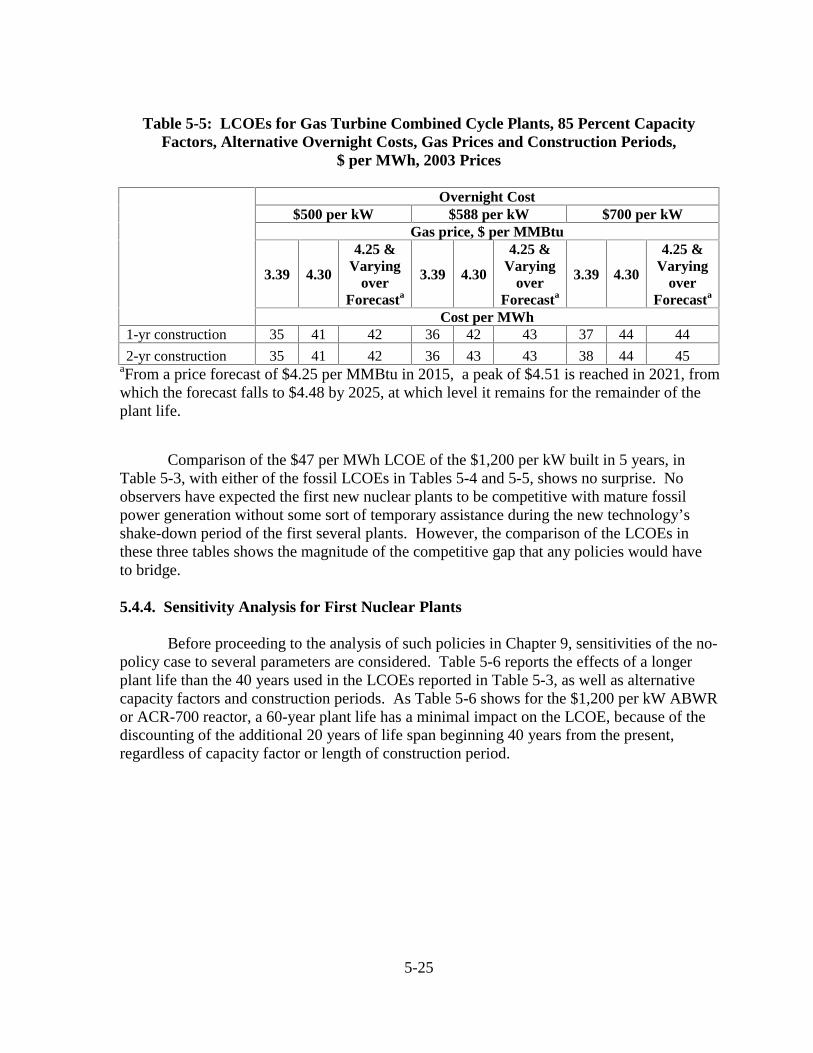
5-25

Table 5-5: LCOEs for Gas Turbine Combined Cycle Plants, 85 Percent CapacityFactors, Alternative Overnight Costs, Gas Prices and Construction Periods,

$ per MWh, 2003 Prices

Overnight Cost$500 per kW $588 per kW $700 per kW

Gas price, $ per MMBtu

3.39 4.30

4.25 &Varying

overForecasta

3.39 4.30

4.25 &Varying

overForecasta

3.39 4.30

4.25 &Varying

overForecasta

Cost per MWh1-yr construction 35 41 42 36 42 43 37 44 44

2-yr construction 35 41 42 36 43 43 38 44 45aFrom a price forecast of $4.25 per MMBtu in 2015, a peak of $4.51 is reached in 2021, fromwhich the forecast falls to $4.48 by 2025, at which level it remains for the remainder of theplant life.

Comparison of the $47 per MWh LCOE of the $1,200 per kW built in 5 years, inTable 5-3, with either of the fossil LCOEs in Tables 5-4 and 5-5, shows no surprise. Noobservers have expected the first new nuclear plants to be competitive with mature fossilpower generation without some sort of temporary assistance during the new technology’sshake-down period of the first several plants. However, the comparison of the LCOEs inthese three tables shows the magnitude of the competitive gap that any policies would haveto bridge.

5.4.4. Sensitivity Analysis for First Nuclear Plants

Before proceeding to the analysis of such policies in Chapter 9, sensitivities of the no-policy case to several parameters are considered. Table 5-6 reports the effects of a longerplant life than the 40 years used in the LCOEs reported in Table 5-3, as well as alternativecapacity factors and construction periods. As Table 5-6 shows for the $1,200 per kW ABWRor ACR-700 reactor, a 60-year plant life has a minimal impact on the LCOE, because of thediscounting of the additional 20 years of life span beginning 40 years from the present,regardless of capacity factor or length of construction period.

5-26

Table 5-6: Effects of Capacity Factor, Construction Period, and Plant Life on First-Plant Nuclear LCOE for Three Reactor Costs, $ per MWh, 2003 Prices

Overnight CostCapacityFactor,Percent $1,200 per kW $1,500 per kW $1,800 per kW

5-year construction periodPlant Life Plant Life Plant Life

40 years 60 years 40 years 60 years 40 years 60 years85 47 47 54 53 62 61

90 44 43 51 50 58 58

95 42 41 49 48 56 55

7-year construction periodPlant Life Plant Life Plant Life

40 years 60 years 40 years 60 years 40 years 60 years85 53 53 62 61 71 70

90 50 49 58 58 67 66

95 47 47 56 55 64 63

With an 85 percent capacity factor, the additional 20 years of plant life reduces theLCOE of the $1,200 per kW plant by $0.72 per MWh if it can be built in 5 years, or by $0.79per MWh if construction takes 7 years. The $1,500 and $1,800 per kW plants experiencesimilar impacts.

Capacity factor adds directly to the ability to produce revenue. The base capacityfactor of 85 percent may appear low relative to recently achieved availability levels in U.S.nuclear plants, in the range of 90 to 92 percent. Some questions have been raised whetherthose high levels are sustainable, and it is worth considering that capacity factor in a newlyopened plant may be something below its long-term operating level, which would have alarge effect on discounted revenues and correspondingly raise LCOE. Table 5-6 also reportsthe sensitivity of the LCOEs of Table 5-3 to variations in capacity factor, from 85 percentthrough 95 percent, for 5- and 7-year construction periods. The $1,200 per kW plant couldachieve an LCOE as low as $42 per MWh with a 95 percent capacity factor, if the plantcould be built in 5 years.

Lengthening the debt term reduces the LCOE. The upper line in Figure 5-1 shows theLCOE of a first $1,500 per kW plant, built in 7 years, with debt terms ranging from 10 yearsto 40 years. Varying the debt term by 30 years from a short term of 10 years to a long termof 40 can reduce the LCOE by a little more than 10 percent. While addressing suchfinancing structure can help keep the LCOE down, by itself it is not a panacea.

5-27

The lower line of Figure 5-1 supposes that each cost and performance parameter is atits most optimistic value and examines the effect of changing the debt term. This calculationis for a plant built in 5 years, at $1,200 per kW overnight cost, with 60 percent debt and40 percent equity, and expecting a 60-year operating life. Debt and equity interest ratesremain at 10 and 15 percent. The LCOE with a 25-year debt term is $40 per MWh, andextending the debt term to 40 years by only another $1.50 per MWh, to $39 per MWh. Thisis close to the range of gas-fired power, but the combination of cost and performanceassumptions is probably too optimistic for a first plant. Nonetheless, the ability of shiftingthe basic cost and performance parameters within a range of values that may be realistic for alater plant offers promise for the commercial viability of some nth plant in the future.

Figure 5-1: The Effect of Debt Term: First-Plant LCOEs for a $1,500 per kW,AP1000, and $1,200 per kW Plant with Reduced Construction Time and Higher Debt

Ratio, $ per MWh, 2003 Prices

$35

$40

$45

$50

$55

$60

$65

10 15 20 25 30 35 40

Base OptimisticDebt Term, years

The impact of construction delays is addressed in Table 5-7. The $1,500 per kWreactor design is chosen for illustration. Two cases are considered in a 7-year constructionperiod. The first row of the table reports the LCOE with no construction delays. The secondrow reports the impact of a 2-year hiatus in construction coming in the middle of theconstruction period, and the bottom row places the delay after 7 years, when all constructionoutlays have been expended but power sales from the plant have not been allowed to begin.

A 2-year delay in the middle of the construction would increase the interestcomponent of total capital costs enough to raise the LCOE 12 percent above what it would bein the absence of delays—from $62 to $69 per MWh. A comparable period of delay after all

5-28

expenditures have been put out at interest would raise the LCOE by 24 percent. Theseriousness of construction delays for economic viability cannot be underestimated.

Table 5-7: The Impact of Construction Delays on the First-Plant LCOE of a $1,500 perkW Plant, $ per MWh, 2003 Prices

No delay 62Delay in middle of construction period 69Delay after end of construction period 76

An inflation rate of 3 percent is used in all LCOE calculations. Experimentationindicates some sensitivity of the real LCOE to the inflation rate. To keep the real interest rateconstant, when varying the inflation rate, a corresponding adjustment is made in the interestrates. For example, to experiment with a 2 percent inflation rate from a base rate of 3percent, 1 percentage point is subtracted from the debt and equity interest rates. Reducingthe inflation rate from 3 percent to 2 percent in this manner reduces LCOE by a little lessthan 4.5 percent.

5.5. Conclusion

The analysis here indicates that reasonable variations in the cost and performanceparameters of new reactor designs do not appear able to bring these new plants fully into thecompetitive range of generation costs, although the variations do help materially. Reducingthe construction period of a plant with $1,500 per kW overnight cost from 7 years to 5,extending plant life, and rearranging the debt term of the financing all reduce the nuclearLCOE, the lowest-cost nuclear cases remain just above the highest-cost coal and gas cases.Increasing capacity factor, for any given capital cost and construction time, from 85 to 95percent would decrease LCOE by a little less than 10 percent. The results here are for firstnew plants coming on line in 2015. The effects of learning by doing and favorableconstruction and operating outcomes on LCOEs of subsequent plants will be considered inChapter 9.

5-29

References

Alliant Energy. (2004) “Power Iowa – Emery Generating Station.” Newsroom, CurrentIssues. Retrieved May 2004, from the World Wide Web:http://www.alliantenergy.com/stellent/groups/public/documents/pub/news_ci_pi_011130.hcsp.

Altman, Edward I., and Vellore M. Kishore. (1998) “Defaults and Returns on High YieldBonds: Analysis Through 1997.” Working Paper. New York: NYU Salomon Center.

Antoniou, Antonios, Yilmaz Guney, and Krishna Paudyal. (2002) “The Determinants ofCorporate Debt Maturity Structure.” Working paper, Centre for Empirical Research inFinance, Department of Economics and Finance, University of Durham, version 1.4,December 12.

Armistead, Thomas F., and Jonathan Barnes. (2002) “Coal Gets New Respect,” November18. Retrieved May 2004 from the World Wide Web: http://enr.construction.com.

Bali, Geetanjali, and Frank S. Skinner. (2003) “The At-Issue Maturity of Corporate Bonds:The Influence of Credit Rating, Security Level, Duration and Macroeconomic Conditions.”ISMA Discussion Papers in Finance 2003-01, International Securities Market Association,University of Reading.

Banz, Rolf W. (1981) “The Relationship Between Return and Market Value of CommonStocks,” Journal of Financial Economics 9: 3-18.

Barclay, M.J., and Clifford W. Smith, Jr. (1995) “The Maturity Structure of Corporate Debt,”Journal of Finance 50: 609-631.

Barrett, W. Brian, Andrea J. Heuson, and Robert W. Kolb. (1986) “The Effect of Three MileIsland on Utility Bond Risk Premia: A Note,” Journal of Finance 41: 255-261.

Belkaoui, Ahmed. (1975) “A Canadian Survey of Financial Structure,” FinancialManagement 4: 74-79.

Benmelech, Efraim. (2003) “Asset Salability and Debt Maturity: Evidence from 19thCentury American Railroads.” Working paper, Graduate School of Business, University ofChicago, October.

Berger, Allen N., Marco Espinosa-Vega, W. Scott Frame, Nathan H. Miller. (2003) “DebtMaturity, Risk, and Asymmetric Information.” Mimeo, preliminary draft, Federal ReserveBoard and International Monetary Fund, January.

Black, Fischer and Myron S. Scholes. (1973) “The Pricing of Options and CorporateLiabilities,” Journal of Political Economy 81: 637-654.

5-30

Black, Fischer, Michael C. Jensen, and Myron S. Scholes. (1972) “The Capital Asset PricingModel: Some Empirical Tests,” in Michael C Jensen, ed., Studies in the Theory of CapitalMarkets. New York: Praeger, pp. 79-121.

Black, Fischer. (1972) “Capital Market Equilibrium with Restricted Borrowing,” Journal ofBusiness 45: 444-455.

Bloomberg, Inc. (2004). Bloomberg Financial Data. March. Retrieved from World WideWeb March 2004: http://www.bloomberg.com/index.html.

Bowen, Robert M., Lane A. Daley, and Charles C. Huber, Jr. (1982) “Evidence on theExistence and Determinants of Inter-Industry Differences in Leverage,” FinancialManagement 11: 10-20.

Bowen, Robert M., R. Castanias, and Lane A. Daley. (1983) “Intra-Industry Effects of theAccident at Three Mile Island,” Journal of Financial and Quantitative Analysis 18: 87-110.

Bradley, Michael, Gregg A. Jarrell, and E. Han Kim. (1984) “On the Existence of an OptimalCapital Structure: Theory and Evidence,” Journal of Finance 39: 857-880.

Brick, Ivan E., and Oded Palmon. (1992) “Interest Rate Fluctuations and the Advantage ofLong-Term Debt Financing : A Note on the Effect of the Tax Timing Option,” FinancialReview 27: 467-474.

Brick, Ivan E., and S. Abraham Ravid. (1985) “On the Relevance of Debt MaturityStructure,” Journal of Finance 40: 1423-1437.

Brick, Ivan E., and S. Abraham Ravid. (1991) “Interest Rate Uncertainty and the OptimalDebt Maturity Structure,” Journal of Financial and Quantitative Analysis 26: 63-81.

Bristol (Va.) Herald Courier. (2004) “Governor Signs Meth Bill,” April 16. Retrieved May2004, from the World Wide Web:http://www.mapinc.org/drugnews/v04/n594/a04.html?66704.

Brooks, L., and R. D’Souza. (1982) “Electric Utility Returns and Risk in the Light of ThreeMile Island,” Public Utilities Fortnightly, November 11, 26-32.

Buckland, Roger, and Patricia Fraser. (2001) “Political and Regulatory Risk: BetaSensitivity in U.K. Electricity Distribution,” Journal of Regulatory Economics 19: 5-25.

Calpine Corporation. (2001) “New Power Plant in Bastrop Begins Operations in Time forSummer Demands.” Press release, June 4. Retrieved May 2004 from the World Wide Web:http://www.corporate-ir.net/ireye/ir_site.zhtml?ticker=CPN&script=411&layout=-6&item_id=180275.

5-31

Chen, Chao, Philp Fanara, Jr., and Raymond F. Gorman. (1987) “Abandonment Decisionsand the Market Value of the Firm: The Case of Nuclear Power Project Abandonment,”Journal of Accounting and Public Policy 6: 285-297.

Das, S. and P. Tufano. (1996) “Pricing Credit Sensitive Debt when Interest Rates and CreditSpreads are Stochastic,” Journal of Financial Engineering 5: 161-198.

Diamond, Douglas W. (1991) “Debt Maturity Structure and Liquidity Risk,” QuarterlyJournal of Economics 106: 709-738.

Diamond, Douglas W. (1993) “Seniority and Maturity of Debt Contracts,” Journal ofFinancial Economics 33: 341-368.

Diamond, Douglas W., and Raghuram G. Rajan. (2001) “Banks, Short-term Debt andFinancial Crises: Theory, Policy Implications and Applications,” Carnegie-RochesterConference Series on Policy 54: 37-71.

Dominion Energy. (2001) “Dominion Plans $600 Million Power Station in Person County.”News release, September 28. Retrieved May 2004, from the World Wide Web:http://www.dom.com/news/dom2001/pr0928.jsp.

Dominion Energy. (2004) Personal communication. Corporate CommunicationsDepartment, Richmond, Va., May 26.

Douglas, George W. (1969) “Risk in the Equity Markets: An Empirical Appraisal of MarketEfficiency,” Yale Economic Essays 9: 2-45.

Drennan, Thomas E., Arnold B. Baker, and William Kamery. (2002) Electricity GenerationCost Simulation Model (GenSim). SAND2002-3376. Albuquerque, N.M.: Sandia NationalLaboratories, November.

Duffie, D., and K. Singleton. (1997) “Modeling Term Structures of Defaultable Bonds,”Review of Financial Studies 12: 687-720.

Duffee, G. (1998) “The Relation Between Treasury Yields and Corporate Bond YieldSpreads,” Journal of Finance 53: 2225-2241.

Elyasiani, Elyas, Lin Guo, and Liang Tang. (2002) “The Determinants of Debt Maturity atIssuance: A System-Based Model,” Review of Quantitative Finance and Accounting 19:351-377.

Elton, Edwin J., Martin J. Gruber, Deepak Agrawal, and Christopher Mann. (2001)“Explaining the Rate Spread on Corporate Bonds,” Journal of Finance 56: 247-277.

5-32

Energy Info Source. (2003) “MidAmerican Energy Begins Work on High-Tech GenerationPlant,” September 9. Retrieved May 2004, from the World Wide Web:http://www.energyinfosource.com/aoi/news-details.cfm?id=19974&FLink=&tf=1.

Fama, Eugene F. (1965) “Portfolio Analysis in a Stable Paretian Market,” ManagementScience 11: 404-419.

Fama, Eugene, and Kenneth French. (1992) “The Cross Section of Expected StockReturns,” Journal of Finance 47: 427-465.

Fama, Eugene F., and Kenneth R. French. (2002) “Testing Trade-off and Pecking OrderPredictions,” Review of Financial Studies 15: 1-33.

Fama, Eugene F., and Kenneth R. French. (2003) “Financing Decisions: Who Issues Stock ?”Mimeo. Chicago, IL.: University of Chicago Graduate School of Business, October.

Fama, Eugene, and James MacBeth. (1973) “Risk, Return, and Equilibrium,” Journal ofPolitical Economy 81: 607-636.

Farber, Stephen. (1991) “Nuclear Power, Systematic Risk, and the Cost of Capital,”Contemporary Policy Issues 9: 73-82.

Fisher, Edwin O., Robert Heinkel, and Josef Zechner. (1989) “Dynamic Capital StructureChoice: Theory and Test,” Journal of Finance 44: 19-40.

Fisher, Larry. (1966) “Some New Stock Market Indexes,” Journal of Business 39: 191-225.

Flannery, M. (1986) “Asymmetric Information and Risky Debt Maturity Choice,” Journalof Finance 41: 18-38.

Fons, Jerome S., Kimball, Andrew E. (1991) “Corporate Bond Defaults and Default Rates,1970-90,” Journal of Fixed Income 1, No. 1: 36-47.

Fraser, Donald R., and James W. Kolari. (1983) “Effects of Three Mile Island on Nuclearand Non-Nuclear Dependent Utilities,” Journal of the Midwest Finance Association 12:1285-1292.

Fuller, Russell J., George W. Hinman, and Thomas C. Lowinger. (1990) “The Impact ofNuclear Power on the Systematic Risk and Market Value of Electric Utility Common Stock,”The Energy Journal 11, No. 2: 117-133.

Galai, D., and R. Masulis. (1976) “The Option Pricing Model and the Risk Factor of Stock,”Journal of Financial Economics 3: 53-81.

5-33

Generation Markets Week. (2002) “Mississippi Merchant Plant Generation,” Power Daily,September 3. Retrieved May 2004, from the World Wide Web:www.aengblom.com/docs/GMW02-09-03Miss.pdf.

Ghosh, Arvin, Francis Cai, and Wenhui Li. (2000) “The Determinants of Capital Structure,”American Business Review 29: 129-132.

Graham, John R., and Campbell R. Harvey. (2001) “The Theory and Practice of CorporateFinance: Evidence from the Field,” Journal of Financial Economics 60: 187-243.

Guedes, Jose, and Tim Opler. (1996) “The Determinants of the Maturity of Corporate DebtIssues,” Journal of Finance 51: 1809-1833.

Hamilton, David T. (1999) “August Default Report,” Moody’s Risk Management ServicesSeptember, p. 3.

Hearth, Douglas, Ronald W. Melichor, and Darryl E. J. Gurley. (1990) “Nuclear Power PlantCancellations: Sunk Costs and Utility Stock Returns,” Quarterly Journal of Business andEconomics 29, no. 1: 102-116

Hewlett, J. (1984) “Investor Perceptions of Nuclear Power.” Washington, D.C.: DOE/EIA-0446. Energy Information Agency, U.S. Department of Energy, May.

Hill, Joanne, and Thomas Schneeweis. (1983) “The Effect of Three Mile Island on ElectricUtility Stock Prices: A Note,” Journal of Finance 38: 1285-1292.

Hogan, William W. (2002) “Electricity Market Restructuring: Reform of Reforms,”Journal of Regulatory Economics 21: 103-132.

Houston Business Journal. (2001) “Reliant Starts Miss. Power Plant Construction,” October8. Retrieved May 2004, from the World Wide Web:http://www.bizjournals.com/houston/stories/2001/10/08/daily4.html.

Hull, Robert M. (1999) “Leverage Ratios, Industry Norms, and Stock Price Reaction: AnEmpirical Investigation of Stock-for-Debt Transactions,” Financial Management 28: 32-45.

Ishii, Jun, and Jingming Yan. (2004) “Investment under Regulatory Uncertainty: U.S.Electricity Generation Investment since 1996.” Working Paper, Center for the Study ofEnergy Markets. Berkeley: University of California Energy Institute, March.

Jarrow, R., D. Lando, and S. Turnbull (1997) “A Markov Model for the Term Structure ofCredit Spreads,” Review of Financial Studies 10: 481-523.

Jensen, Michael, and William Meckling. (1976) “Theory of the Firm: Managerial Behavior,Agency Costs, and Capital Structure,” Journal of Financial Economics 3: 305-360.

5-34

Johnson, Ramon E. (1967) “Term Structures of Corporate Bond Yields as a Function ofRisk of Default,” Journal of Finance 22: 313-345.

Jones, E. Philip, Scott P. Mason, and Eric E. Rosenfeld, and Lawrence Fisher. (1984)“Contingent Claims of Analysis of Corporate Capital Structures: An EmpiricalInvestigation,” Journal of Finance 39: 611-625.

Joskow, Paul L. (1997) “Restructuring, Competition and Regulatory Reform in the U.S.Electricity Sector,” Journal of Economic Perspectives 11: 119-138.

Ju, Nengjiu, and Hui Ou-Yang. (2003) “A Dynamic Model of Optimal Capital Structure andDebt Maturity with Stochastic Interest Rates.” Working paper, December 15.

Kale, J. R., and T. Noe. (1990) “Risky Debt Maturity Choice in a Sequential GameEquilibrium,” Journal of Financial Research 13: 155-165.

Kale, Jayant R., Thomas H. Noe, and Gabriel G. Ramìrez. (1991) “The Effect of BusinessRisk on Corporate Capital Structure: Theory and Evidence,” Journal of Finance 46: 1693.

Kalra, Rajiv, Glenn V. Henderson, Jr., and Gary A. Raines, (1993) “Effects of the ChernobylNuclear Accident on Utility Share Prices,” Quarterly Journal of Business and Economics 32:52-77.

Kane, A., A. J. Marcus, and R. L. McDonald. (1985) “Debt policy and the rate of returnpremium to leverage,” Journal of Financial and Quantitative Analysis 20: 479-499.

Kim, C.S., D.C. Mauer, and M. H. Stohs. (1995) “Corporate Debt Maturity Policy andInvestor Tax-timing Options: Theory and Evidence,” Financial Management 24: 33-45.

LaBar, Malcolm (2002) “The Gas Turbine-Modular Helium Reactor: A Promising Option forNear Term Deployment.” San Diego, Ca.: General Atomics. Retrieved December 13, 2003from the World Wide Web: http://www.ga.com/gtmhr/images/ANS.pdf.

Lando, D. (1997) “Some Elements of Rating-Based Credit Risk Modeling,” in N. Jegadeeshand B. Tuckman, eds., Advanced Tools for the Fixed Income Professional. New York:Wiley, pp. 193-215.

Lee, W. Y., A. V. Thakor, and G. Vora. (1983) “Screening, Market Signaling and CapitalStructure Theory,” Journal of Finance 38: 1507-1518.

Leland, H. E., and K. B. Toft. (1996) “Optimal Capital Structure, Endogenous Bankruptcy,and the Term Structure of Credit Spreads,” Journal of Finance 51: 987-1019.

5-35

Lescoeur, Bruno, and Philippe Penz. (1999) La problématique du financement duinvestissements électronucléaires,” Revue de économie financi�re 51: 167-182.

Lignite Energy Council. (2004). “Energy Success Story, King Plant Readies for NewEmissions Control Technology,” February. Retrieved May 2004, from the World WideWeb: http://www.lignite.com/ess/feb_04.html.

Lintner, John. (1965) “The Valuation of Risk Assets and the Selection of Risky Investmentsin Stock Portfolios and Capital Budgets,” Review of Economics and Statistics 47: 13-37.

Longstaff, Francis, and E. Schwartz. (1995) “A Simple Approach to Valuing Risky Fixedand Floating Rate Debt,” Journal of Finance 50: 789-819.

Madan, D. B., and H. Unal (1998) “Pricing the Risks of Default,” Review of DerivativesResearch 2: 121-160.

Markowitz, Harry M. (1959) Portfolio Selection: Efficient Diversification of Investments.New York: Wiley.

Marsh, Paul. (1982) “The Choice Between Equity and Debt: An Empirical Study,” Journal ofFinance 37: 121-144 .

Martin, Linda J., and Glenn V. Henderson. (1984) “Industry Influence on FinancialStructure: A Matter of Interpretation,” Review of Business and Economic Research 19: 57-67.

Mazur, Frank. (2003), commentary, “Nature’s Power: Blowing in the Wind,” RepresentativeFrank Mazur’s (Vermont) Home Page. Retrieved May 2004, from the World Wide Web:http://home.adelphia.net/~frankmazur/windmills_10_03.htm.

Merchant Power Monthly. (2004a) “As Natural Gas Surges, Illinois Utilities Turn to Coal toFuel Power Plants,” Vol. 19, no. 4 (April), pp. 2-3.

Merchant Power Monthly. (2004b) “Boston-Based Firm Delays Building Natural-Gas-FiredPlant in North Carolina,” Vol. 19, no. 4 (April), p. 9.

Merton, Robert. (1997) “On the Pricing of Corporate Debt: The Risk Structure of InterestRates,” Journal of Finance 29: 449-470.

Midwest Generation. (2004) Personal communication. Government Affairs Department,Chicago, May 26.

Miller, Merton, and Myron Scholes. (1972) “Rates of Return in Relation to Risk: A Re-Examination of Some Recent Findings,” in Michael Jensen, editor, Studies in the Theory ofCapital Markets. New York: Praeger, pp. 47-78.

5-36

Minnesota Environmental Partnership. (2004) “Once-King Coal Returns to the Midwest.”Environmental News, May 5. Retrieved from World Wide Web May 2004:http://www.mepartnership.org/mep_whatsnew.sap?new_id=651.

Mitchell, Karlyn. (1991) “The Call, Sinking Fund, and Term to Maturity Features ofCorporate Bonds: An Empirical Investigation,” Journal of Financial and QuantitativeAnalysis 26: 201-222.

Modigliani, Franco, and Merton H. Miller. (1958) “The Cost of Capital, CorporationFinance, and the Theory of Investment,” American Economic Review 48: 261-297.

Morris, J. R. (1976) “On Corporate Debt Maturity Policies,” Journal of Finance 31: 29-37.

Morris, J. R. (1992) “Factors Affecting the Maturity Structure of Corporate Debt.” Workingpaper, University of Colorado at Denver.

Mossin, Jan. (1966) “Equilibrium in Capital Markets,” Econometrica 34: 768-783.

Myers, Stewart. (1977) “Determinants of Corporate Borrowing,” Journal of FinancialEconomics 9: 147-176.

Myers, Stewart C. (1984) “The Capital Structure Puzzle,” Journal of Finance 39: 575-592.

Myers, Stewart C., and Nicholas S. Majluf. (1984) “Corporate Financing and InvestmentDecisions when Firms have Information that Investors Do Not Have,” Journal of FinancialEconomics 13: 187-221.

Nebraska Public Power District. (2003) “Power Plant Construction Begins” News release,June 26. Retrieved May 2004, from the World Wide Web:http://www.nppd.com/News/News_Releases/2003/Additional_Files/construction.asp

Nebraska Public Power District. (2004) Personal communication. CorporateCommunications Department, Columbus, Nebr., May 26.

Nielson, Mark. (1993) Investigation Costs and the Effects of Own Variance on SecurityPrices. Ph.D. dissertation, University of Chicago, Department of Economics.

NRG Energy. (2004) Personal communication. Media Relations Department, Minneapolis,May 27.

Nwaeze, Emeka T. (2000) “Deregulation of the Electric Power Industry: The Earnings,Risk, and Return Effects,” Journal of Regulatory Economics 17: 49-67.

5-37

Pacific Northwest National Laboratory (PNNL). (2004) State Electricity RestructuringStatus. Retrieved March 2004 from the World Wide Web: http://pnnl-utilityrestructuring.pnl.gov/Electric/electric.htm.

Pindyck, Robert S. (1993) “Investments of Uncertain Cost,” Journal of Financial Economics34: 53-76.

Peabody Energy. (2004) Personal communication. Public Relations Department, St. Louis,May 25.

Ravid, Abraham. (1996) “Debt Maturity: A Survey,” Financial Markets, Institutions andInstruments 5: 1-68.

Realdon, Marco. (2003) “About Debt and the Option to Extend Debt Maturity.” DiscussionPapers in Economics, No. 2003/20, Department of Economics and Related Studies,University of York.

Remmers, Lee, Arthur Stonehill, Richard Wright, and Theo Beekhuisen. (1974) “Industryand Size as Debt Ratio Determinants in Manufacturing Internationally,” FinancialManagement 3: 24-32.

Reuters. (2001) “Record Gas Prices Breathe Life Into Nuclear Power,” January 25.Retrieved May 2004 from the World Wide Web:https://www.pbmr.co.za/press_archive/record_gas_prices.htm.

Reuters (2004) “Reliant to Mothball Miss. Power Plant,” News for RRI.N., May 4. RetrievedMay 2004 from the World Wide Web: http://biz.yahoo.com/prnews/040504/datu041_1.html.

Roll, Richard, and Stephen A. Ross. (1980) “An Empirical Investigation of the ArbitragePricing Theory,” Journal of Finance 35: 1073-1103.

Rosenberg, B., K. Reid, and R. Lanstein. (1985) “Persuasive Evidence of MarketInefficiency,” Journal of Portfolio Management 11: 9-17.

Rousseau, Fabrice. (1999) “Signaling with Debt Maturity Choice.” Working paper,National University of Ireland, Maynooth, November.

Sargent & Lundy. (2004) Personal communication. Fossil Power Department, Chicago,May 24.

Sarkar, Sudipto. (1999) “Illiquidity Risk, Project Characteristics, and the Optimal Maturityof Corporate Debt,” Journal of Financial Research 22: 353-370.

Schwartz, Eli, and J. Richard Aronson. (1967) “Some Surrogate Evidence in Support of theConcept of Optimal Financial Structure,” Journal of Finance 22: 10-18.

5-38

Scott, David F. (1972) “Evidence on the Importance of Financial Structure,” FinancialManagement 1: 45-50.

Scott, David F., and John D. Martin. (1975) “Industry Influence on Financial Structure,”Financial Management 4: 67-73.

Scully Capital. (2002a) Business Case for New Nuclear Power Plants. Final Draft.Washington, D.C.: Scully Capital, July. Retrieved December 2003 from the World WideWeb: http://www.scullycapital.com.

Scully Capital. (2002b) “BCNPP: Business Case for New Nuclear Power Plants; Briefingfor NERAC.” Retrieved December 13, 2003 from the World Wide Web:http://nuclear.gov/home/bc/ExecOverviewNERAC100102.pdf.

Sekely, William S., and J. Markham Collins. (1988) “Cultural Influences on InternationalCapital Structure,” Journal of International Business Studies 19: 87-100.

Sharpe, Steven. (1991) “Credit Rationing, Concessionary Lending, and Debt Maturity,”Journal of Banking and Finance 15: 581-604.

Sharpe, William F. (1964) “Capital Asset Prices: A Theory of Market Equilibrium UnderConditions of Risk,” Journal of Finance 19: 425-442.

The Shaw Group. (2001) “Shaw Signs Agreement with NRG Energy for Power PlantConstruction.” Press release, September 27. Retrieved May 2004 from the World WideWeb: http://www.shawgrp.com/press_Releases/2001/092701.cfm.

Sibley, Mike. (1991) “The Search for Industry Financing Patterns,” American BusinessReview, January: 85-91.

Smith, Richard, and Anders Hove. (2003) “The Old Reliables: Coal, Nuclear and Gas in2003.” New York: Deutsche Bank AG.

Sommers, Paul. (1980) “The Adoption of Nuclear Power Generation,” Bell Journal ofEconomics and Management 11: 283-291.

Stattman, D. (1980) “Book Values and Stock Returns,” The Chicago MBA: A Journal ofSelected Papers 4: 25-45.

Stohs, Mark Hoven, and David C. Mauer. (1996) “The Determinants of Corporate DebtMaturity,” Journal of Business 69: 279-312.

Titman, Sheridan. (1992) “Interest Rate Swaps and Corporate Financing Choices,” Journalof Finance 47: 1503-1516.

5-39

Titman, Sheridan, and R. Wessels. (1988) “The Determinants of Capital Structure Choice,”Journal of Finance 43: 1-19.

Tolley, George, and Mark Nielson. (1992) “Asset Pricing with Investigation Costs.” Mimeo.University of Chicago, March.

Tolley, George, and Mark Nielson. (2003) “Asset Pricing with Information Costs.” Mimeo,University of Chicago and MacroEcon Global Advisors, working paper, July.

Tyler Morning Telegram. (2004) “Clean-Air Efforts Threatened, Environmentalists Say,”March 2. From Typerpaper.com. Retrieved May 2004, from the World Wide Web:http://www.zwire.com/site/news.cfm?newsid=11055212&BRD=1994&PAG=461&dept.

U.S. Department of Energy (DOE). (2001a) “A Roadmap to Deploy New Nuclear PowerPlants in the United States by 2010, Volume I.” Summary Report. Washington, D.C.: Officeof Nuclear Energy, Science and Technology, October.

U.S. Department of Energy (DOE). (2001b) “A Roadmap to Deploy New Nuclear PowerPlants in the United States by 2010, Volume II.” Main Report. Washington, D.C.: Office ofNuclear Energy, Science and Technology, October.

U.S. Department of the Treasury, Internal Revenue Service (IRS). (2002) “How toDepreciate Property.” Publication 946. Washington, D.C.: IRS.

Uselton, Gene C., James W. Kolari, and Donald R. Fraser. (1986) “Long-Term Trends in theRiskiness of Electric Utility Shares,” Journal of Business Finance and Accounting 13: 453-459.

Wiggins, James B. (1990) “The Relation Between Risk and Optimal Debt Maturity and theValue of Leverage,” Journal of Financial and Quantitative Analysis 25: 377-386.

Wisconsin Public Service Corporation. (2002) “WPS Resources Corporation DiscussesFinancial Details of Wisconsin Public Service Corporation Building a 500-Megawatt Coal-Fired Electric Generator.” WPS Resources Corporation, September 25. Retrieved May 2004from the World Wide Web: http://www.wpsr.com/cfm/smwpsr.gif.

Xcel Energy. (2004) Personal communication. Capital Projects, Engineering andConstruction Department, Minneapolis. May 24.

5-40

Part Two: Outlook for Nuclear Energy’s Competitors

Part Two considers the prospects for gas and coal as the major baseload competitorsto nuclear generation. Consideration is given to technologies that could reduce costs of gas-and coal-fired electricity, fuel price changes that could affect relative competitiveness, andthe potential effect of greenhouse gas controls on costs of fossil-fuel generation.

6-1

Chapter 6. GAS AND COAL TECHNOLOGIES

Summary

This chapter examines the near-term prospects for improvements in gas- and coal-fired electricity generation that would affect their costs relative to nuclear power. Somemodest efficiency improvements are foreseen in the near term for gas technologies, but theprospects for coal technologies appear to be farther in the future.

The most common combustion technology used in recently constructed coal plants inthe United States is pulverized coal combustion (PCC). The thermal efficiency of mostfluidized beds used for power generation is similar to that of conventional PCC plants.Interest in the use of this technology has been stimulated by its better environmentalperformance even when utilizing lower grade fuels. However, its cost competitivenessremains in question. Integrated coal gasification combined cycle (IGCC), while attractivefrom a thermal efficiency and emissions perspectives, is likely to be too expensive to enterthe U.S. market in the near term.

More advanced coal-fired technologies are still in early R&D stages. Since little canbe said about their near-term commercialization potentials, they are not included as realisticpossibilities for reducing coal-fired generation costs within the time scope of the presentstudy.

The primary gas-fired technology for new baseload electricity generation is gasturbine combined cycle. Modern gas turbine plants with a triple-pressure heat recoverysteam generation (HRSG) system with steam reheat can reach thermal efficiencies above55 percent. A gas turbine, with steam cooling of the turbine blades and nozzles, combinedwith an advanced HRSG is expected to operate at an efficiency level of 60 percent in the nearfuture. The goal of most world manufacturers is to reach overall thermal efficiencies of thecombined plant of 60 percent in the short term, primarily by increasing firing temperatures.Other cycle improvements could lead to thermal efficiencies nearing 65 percent.

Since fuel costs are generally two-thirds of the levelized cost of gas-generated power,a 5 percentage-point increase in efficiency could result in an approximate by 8 percent costdecrease, which although small, could affect competitive margins across generation types.

6-2

Outline

6.1. Introduction

6.2. Coal-Fired Power Plant Technology

6.2.1. Current and Future Technology6.2.2. Emissions Control Technology6.2.3. Future Power Plant Construction Considerations6.2.4. Cost Estimates

6.3. Gas-Fired Power Plant Technology

6.3.1. Combined Cycle Technology6.3.2. The Future of Gas Turbine Combined Cycle Technology6.3.3. Breakdown of Costs by Capital, Fuel, and O&M6.3.4. Natural Gas Emissions, Control Technology, and Costs6.3.5. Summary of Future Gas Generation Cost Estimates

6.4. Summary of Future Coal and Gas Technologies

References

6-3

6.1. Introduction

Fossil fuel technology continues to be the primary source for electric powergeneration. Moreover, it appears that its market dominance will continue for the foreseeablefuture. Concerns over its environmental impacts have spurred efforts to find alternatives aswell as improve the current technology. The purpose of this chapter is to describe the currentand near future fossil-fired power generation technologies, noting prognoses forimprovements in efficiency and emissions control. Finally, an assessment of the costs for anew coal-fired or gas-fired plant incorporating all necessary emissions control is provided.

6.2. Coal-Fired Power Plant Technology

Since the early 1900s, coal power has provided the bulk of electricity generated in theUnited States because of its low price (Gillenwater 1996, p. 19). Since 1965, the thermalefficiency of steam turbines increased steadily and then plateaued (Gillenwater 1996, p. 21).There has been a general trend toward larger plants to take advantage of scale economies, butthere is a threshold beyond which reliability becomes difficult to ensure in these large units(Gillenwater 1996, p. 21).

6.2.1. Current and Future Technology

6.2.1.1. Pulverized Coal Combustion (PCC)

Pulverized coal combustion (PCC) is the most widely used method for burning coalfor power generation. Older PCC plants offer efficiencies around 30 percent while newersub-critical steam units with high quality coal can reach 35 to 36 percent efficiencies. Newerunits employing supercritical steam may reach efficiencies of 45 percent. However,supercritical boilers are more highly integrated than the simpler sub-critical PCC designs andrequire advanced steel materials. As materials advance, government R&D programs hope toreach efficiencies as high as 50 percent. Further technological improvements depend on thedevelopment of new materials capable of withstanding higher temperatures and pressures(Smith and Hove 2003, p. 39).

6.2.1.2. Fluidized Bed Combustion (FBC)

Fluidized bed boilers were developed in the 1990s and can utilize waste coal thatcould not be burned for power in other boilers (Smith and Hove 2003, p. 41). The advantageof fluidized bed combustion (FBC) is that it encourages complete combustion at a lowertemperature than that of PCC. While the units are cleaner than a corresponding PCC plant,its efficiencies only range from 30 to 35 percent. The most current technology utilizes thepressurized circulating fluidized bed boiler (PCFB) in which the entire combustion chamberis placed under pressure and may deliver higher efficiencies.

6-4

6.2.1.3. Integrated Gasification Combined Cycle (IGCC)

IGCC technology demonstrates 10 to 20 percent more efficiency than conventionalpulverized coal plants, achieves up to 98 percent SO2 removal, and reduces NOX emissions toapproximately 0.1 lb per Btu (DOE 1999, p.17). IGCC plants can obtain efficiency levels of40 to 45 percent with current technologies (Smith and Hove 2003, p. 42). Research anddevelopment projects target 60 percent efficiencies. The immediate technological challengeremains the consumptive nature of the gas clean-up process, which currently requires that thesyngas be cooled before cleaning and ultimate feeding into the turbine (Smith and Hove2003, p. 42).

There is only one gasification plant operating as baseload today in the UnitedStates—Tampa Electric Co.’s Polk Plant, a 250-MW IGCC plant that has been in operationsince 1996 (Alvey 2003, p. 22). However, the experience with current coal-fireddemonstration plants (250 to 300 MW) indicates that additional development is required toreduce capital costs and improve both plant availability and reliability to achieve competitivepower production costs and commercial acceptance.

6.2.1.4. Current Research

Research on coal-fired technologies focused on increasing performance anddecreasing emissions are in early stages. DOE is leading the research effort with its FutureGen, Vision 21, and Advanced Turbine Systems programs (DOE 1999b, p. 12).

6.2.2. Emissions Control Technology

As the use of coal power continues, many of the existing units will be outfitted withenhanced emission controls in the next decade to meet more stringent environmentalregulations for sulfur dioxide (SO2), oxides of nitrogen (NOX), mercury (Hg), particulatematter (PM), and potential greenhouse gases such as carbon dioxide (CO2). These controlsinclude flue gas desulfurization, low-NOX burners (LNBs), selective catalytic reductionsystems (SCR), and particulate matter controls. Moreover, as a result of the New SourceReview provision, all new plants are required to install the best available control technology,which affects coal’s competitiveness with other electric power generation sources. Finally,should carbon sequestration become a requirement in the future, coal power would be put at asignificant disadvantage considering its high carbon content. Carbon sequestration costs arediscussed further in Section 8.3.

6.2.3. Future Power Plant Construction Considerations

The current stock of coal plants is aging and, as a consequence of New SourceReview, is being utilized more intensively. Few coal-fired retirements, re-powering projects,or capacity additions are planned, as utilities and non-utilities show reluctance to assumehigh investment risks (Gillenwater 1996, p. 3). Utility and non-utility companies probablywill not make long-term capital investments as long as the increased demand for electricity at

6-5

coal-fired power plants can be met through extending the life, increasing the utilization ofexisting capital, or both (Gillenwater 1996, p. 3). Additionally, investors generally seelimited opportunities for new baseload capacity in the United States over the next 10 years(EIA 2003, p. 3). Moreover, given the uncertainty over environmental regulation and theneed to minimize long-term capital risk, private companies are unwilling to invest in long-term R&D to improve technology without government support (DOE 1999b, p. 2).

6.2.4. Cost Estimates

6.2.4.1. Mining and Transportation Costs

Continued technological developments for extracting and hauling large volumes ofcoal in both surface and underground mining suggest that further reduction in mining costs islikely. However, EIA expects improvements in labor productivity to remain the key elementto lower coal-mining costs (EIA 2003, p. 87).

In 1997, transportation costs averaged 41 percent of the delivered price of contractcoal shipments to electric utilities. With an increase in the Western market share, an increasein the average shipping distance may lead to increased transportation costs. Rail costs andtransportation bottlenecks lead to regional differences because coal is now being shippedover longer distances (Smith and Hove 2003, p.13). However, EIA projects that rail rates forWestern coal will decline gradually over the next two years with improvements to railroadinfrastructure (Smith and Hove 2003, p. 34).

6.2.4.2. Fuel Supply and Price

Coal is stored in substantial quantities at power plants, and most utility companieshave long-term supply contracts to stabilize coal prices. Consequently most utilities havecontinued to pay low and stable prices for their coal, thereby limiting exposure to the higherprices experienced in 2002. Western coal costs are lower than Eastern costs because of thethickness of the coal seams and high productivity associated with large-scale surface mining,but Western coal tends to have a lower energy content per unit weight than Eastern coal(Smith and Hove 2003, p. 34). Coal supply and price projections are reported in Section 7.2.

6.2.4.3. Capital Costs

Capital costs for new PCC plants range from $1,100 to $1,200 per kW depending ontheir location, and supercritical PCC plants tend to cost closer to $1,200 per kW. PCFBcapital costs are around $1,200 per kW, with somewhat lower gas cleanup costs as part ofthis figure (Smith and Hove 2003, p. 38). DOE estimates the future cost of IGCC units atjust over $1,300 per kW and projects that its price will come down to $1,000 per kW by 2008(Smith and Hove 2003, p. 42).

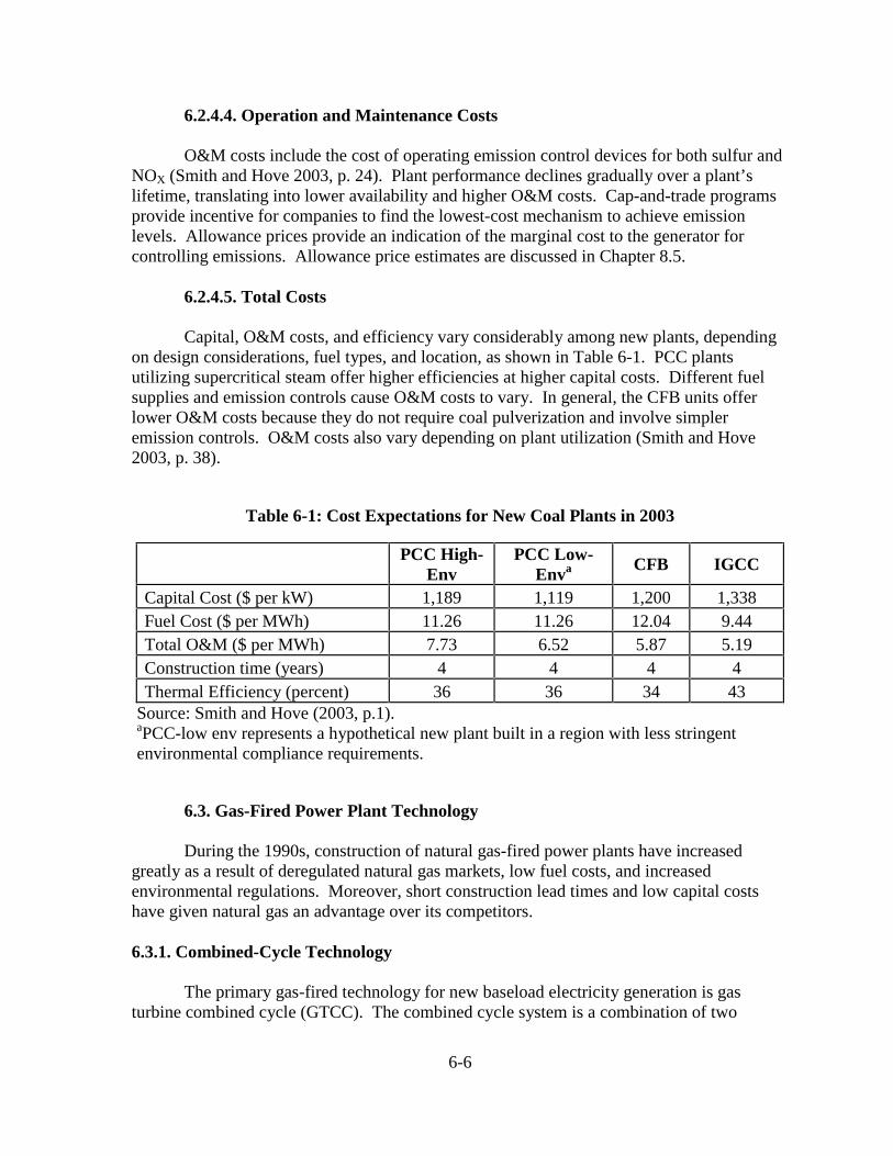
6-6

6.2.4.4. Operation and Maintenance Costs

O&M costs include the cost of operating emission control devices for both sulfur andNOX (Smith and Hove 2003, p. 24). Plant performance declines gradually over a plant’slifetime, translating into lower availability and higher O&M costs. Cap-and-trade programsprovide incentive for companies to find the lowest-cost mechanism to achieve emissionlevels. Allowance prices provide an indication of the marginal cost to the generator forcontrolling emissions. Allowance price estimates are discussed in Chapter 8.5.

6.2.4.5. Total Costs

Capital, O&M costs, and efficiency vary considerably among new plants, dependingon design considerations, fuel types, and location, as shown in Table 6-1. PCC plantsutilizing supercritical steam offer higher efficiencies at higher capital costs. Different fuelsupplies and emission controls cause O&M costs to vary. In general, the CFB units offerlower O&M costs because they do not require coal pulverization and involve simpleremission controls. O&M costs also vary depending on plant utilization (Smith and Hove2003, p. 38).

Table 6-1: Cost Expectations for New Coal Plants in 2003

PCC High-Env

PCC Low-Enva CFB IGCC

Capital Cost ($ per kW) 1,189 1,119 1,200 1,338Fuel Cost ($ per MWh) 11.26 11.26 12.04 9.44Total O&M ($ per MWh) 7.73 6.52 5.87 5.19Construction time (years) 4 4 4 4Thermal Efficiency (percent) 36 36 34 43

Source: Smith and Hove (2003, p.1).aPCC-low env represents a hypothetical new plant built in a region with less stringentenvironmental compliance requirements.

6.3. Gas-Fired Power Plant Technology

During the 1990s, construction of natural gas-fired power plants have increasedgreatly as a result of deregulated natural gas markets, low fuel costs, and increasedenvironmental regulations. Moreover, short construction lead times and low capital costshave given natural gas an advantage over its competitors.

6.3.1. Combined-Cycle Technology

The primary gas-fired technology for new baseload electricity generation is gasturbine combined cycle (GTCC). The combined cycle system is a combination of two

6-7

technologies: the gas turbine and the steam turbine. In a gas turbine, natural gas is burned incombination with a steady stream of high velocity compressed air. The hot combustion gasis then passed through an array of rotating and stationary airfoils that turn a generator toproduce electricity. For the second or bottoming cycle, a heat recovery steam generationsystem (HRSG) and steam turbine are added to take advantage of the thermal energyproduced from the first combustion cycle.

Modern gas turbine plants with a triple-pressure HRSG with steam reheat can reachefficiencies above 55 percent. ABB-Alstom claims 58 percent efficiency of a combinedcycle plant built around its GT24/26 reheat gas turbines; the same efficiency is cited bySiemens, for the Westinghouse steam-cooled W501G/701G gas turbine or V94.3a gasturbine, combined with a triple pressure HRSG. A gas turbine, with steam cooling of theturbine blades and nozzles, combined with an advanced HRSG is expected to operate at anefficiency level of 60 percent in the near future. The goal of most world manufacturers is toreach overall thermal efficiencies of the combined plant of 60 percent in the short term,generally by increasing firing temperatures (Franco 2002, p. 1504).

DOE has recently cited the General Electric (GE) “H” class GTCC system for itsperformance promise. The new system is claimed to reach an overall thermal efficiency of60 percent through its increased gas turbine firing temperature of 1430 degrees C with apressure ratio of 23:1 (Corman 1996, p. 1).

In spite of manufacturer claims of 60 percent efficiency, most industry expertssuggest efficiencies in the range of 55 to 58 percent would be a preferable range to accountfor plant-to-plant variation such as ambient air differences and other environmental factors(Claeson Colpier 2002, p. 313).

6.3.2. The Future of Gas Turbine Combined Cycle Technology

Research into increasing the efficiency of combined-cycle technology is proceedingwith several developments that allow higher firing temperatures, better turbine performance,and more efficient recovery of heat. The engineering literature has paid considerableattention to the optimization of HRSG. Two basic exhaust heat recovery processes can beused to increase efficiency: (1) recuperation, in which the recovered heat is used in the samegas turbine cycle; and (2) bottoming cycle, in which the exhaust is used as a heat source for asecond and essentially independent power producing cycle (Heppenstall 1998, p. 838). Inaddition, basic optimization of HRSG parameters such as mass flow rates and heat exchangerefficiencies can produce substantial increases in overall efficiency. The efficiency increasecan vary from 2 percent for HRSG optimization alone, to 6 to 7 percent using postcombustion reheating, inter-cooling, and gas-to-gas recuperation (Franco 2002, p. 1515).

While significant increases in efficiencies are technically feasible, increasedcomponent and plant complexity could result in increased cost. The thermodynamicperformance of a plant is usually reflected in the fuel cost. The fuel cost savings as a resultof increases in thermal efficiency are shown in Table 6-2, which suggests that, on average, a

6-8

5 percentage-point increase in thermal efficiency will result in an 8 percent reduction in fuelcost. For example, at a 40 percent thermal efficiency, which is equivalent to a heat rate of8,530 per kWh, and a $3.15 per MMBtu cost of gas, the fuel component of the levelized costof electricity (LCOE) of a combined cycle plant would be $27 per MWh.

Table 6-2: Thermal Efficiency Effect on Fuel Cost of GTCC, $ per MWh, 2003 Prices

Fuel Cost Contribution to LCOE,in $ per MWh

At Fuel Pricea, in $ per MMBtu, of:Thermal Efficiency,

PercentHeat Rate,

Btu per kWh3.15 3.75 4.70

40 8530 27 32 4045 7582 24 28 3650 6824 22 26 3255 6204 20 23 2960 5687 18 21 2765 5249 17 20 25

aData generated using fuel price estimates from Smith and Hove (2003) and an average 2009gas contract price from NYMEX (2003).

6.3.3. Breakdown of Costs by Capital, Fuel, and O&M

The cost of generating electricity with gas turbine combined cycles depends not onlyon the capital cost of the plant, but also the cost of fuel, thermal efficiency, load, andoperation and maintenance costs. In addition, differences in national and regional marketcharacteristics and local site conditions can mask the influence of various factors. However,for the purposes of this chapter average values will be used.

Fuel cost is the primary consideration in assessing the LCOE for gas-fired generation.By most estimates it comprises nearly two-thirds of the total cost of generation. As discussedin Section 9.4, the natural gas price has been relatively volatile in recent years due to declinesin productivity and proven reserves, among other, more transient factors. Accordingly,higher fuel prices could cause a reassessment of the economic viability of gas-firedgeneration. Natural gas price models and their forecasts are discussed in Section 7.3.Deutsche Bank suggests average gas prices above $4 per MMBtu in the short run as a criticalpoint at which fuel switching may occur (Smith and Hove 2003a, p. 22). Capital costscomprise less than one-third of the total cost of generation. An average estimate for a newcombined cycle plant is $590 per kW (Smith and Hove 2003a, p. 77). The finalconsideration is the cost of operation and maintenance (O&M), which includes costs ofemission control. Generally gas-fired plants do not require additional pollution controlequipment, which provides a significant O&M cost advantage, but O&M comprises less than6 percent of the LCOE of gas-fired plants (Smith and Hove 2003a, p. 19). Table 6-3 showsDeutsche Bank’s present and future cost projections for gas plants.

6-9

Claeson Colpier et al.’s (2002) analysis suggests that the great reduction in gas-firedelectricity costs through the 1990s was the result of a worldwide increase in installedcapacity and attendant experience with combined cycle technology in electricity generation.If GTCCs become the generation technology of choice, the trend would likely continue,moderated by declining marginal returns to learning, discussed in Chapter 4. According toClaeson Colpier et al., holding the fuel price constant, the stable progress ratio for the cost ofgenerating electricity is approximately 94 percent. That is, at the next point where installedcapacity doubles, the capital cost should fall by 6 percent, or a 6 percent learning effect in theterminology of Chapter 4. The likelihood, however, of a further doubling of capacity in theshort term is small, and therefore its effect on the overall cost of electricity minor comparedto gains in thermal efficiency and fuel cost.

Table 6-3: Cost Estimates for New Gas Plants

2003 Long Terma

Plant Size (MW) 300 300Capital Cost ($ per kW) 590 450Lead Time (Years) 3 3Fuel Price ($ per MMBtu)b 3.75 3.15Fuel Cost ($ per MWh) 23.6 19.9Total O&M Cost ($ per MWh) 2.6 2.6Annual Capital Cost ($ perMWh) 10.2 7.8Levelized Cost ($ per MWh)c 36.4 30.3

Source: Smith and Hove (2003).aLong term is the length of time required for fuel prices to reach an equilibrium, approximately2006 (p. 77).bFuel price based on 2003 EIA estimate, plant efficiency set at 54 percent; price does notinclude post-combustion emissions control.cLevelized cost is the sum of fuel, O&M, and annuitized capital costs.

6.3.4. Natural Gas Emissions, Control Technology, and Costs

When compared with emissions from coal-fired plants, combined cycle plantsproduce significantly less of the six criteria pollutants established by the 1990 Clean Air Act.Natural gas produces no sulfur dioxide or ash, and smaller quantities of volatile organics,CO2, and NOX gases. However, for the purposes of this report, only nitrogen oxides (NOX)will be considered. NOX gas emissions are formed during the combustion of natural gas andother fossil fuels by high temperature oxidation of atmospheric nitrogen. CO2 is a naturalbyproduct of fossil fuel combustion and is currently not a federally regulated gas.

6-10

In general, NOX emissions from gas-fired electricity generation are lower than mostcurrent limits. As discussed in Section 8.5.2., there is regional variation among NOX

standards, and some states such as California and Texas require additional emissions controltechnology. Similarly to coal-based technology, gas-fired generation can employ low-NOX

burners (LNBs) and selective catalytic reduction systems (SCR) to achieve standards as lowas 2.5 parts per million (PPM). In addition, should carbon sequestration be required, itseffect on gas-fired electricity costs probably would be much lower than the effect on coal-fired costs as a result of the lower carbon emissions from natural gas. Carbon emissions arediscussed in more detail in Chapter 8.

6.3.5. Summary of Future Gas Generation Cost Estimates

The future competitiveness of natural gas-fired generation lies in its fuel cost, whichis nearly two-thirds of the overall cost of gas LCOE. Two main factors affect the fuel cost:thermal efficiency and the fuel price. A 5 percentage-point increase in thermal efficiency canreduce the fuel cost by 8 percent. However, the most important cost consideration for gasgeneration remains the fuel price. Since 1998, supply problems have resulted in volatile fuelprices. Table 6-4 shows the sensitivity of gas-fired LCOE to fuel price.

Table 6-4: Effect of Fuel Price on Gas LCOE, $ per MWh

Gas PriceThermal Efficiency,Percent $3.00 $3.40 $3.80 $4.20 $4.60 $5.00

50 33 35 38 41 43 4655 31 33 36 38 41 4360 29 32 34 36 39 41

Source: Smith and Hove (2003).

Assuming the gas supply infrastructure is stabilized in the near term and new supplyoptions such as LNG are realized, the current cost advantage of natural gas generation shouldcontinue. A forecast of the future cost of generation can be calculated using an estimate ofthe fuel price and future thermal efficiency. Assuming that a 5 percentage-point increase inthermal efficiency can be achieved by 2020, the cost of gas-based generation could beexpected to be approximately $30 per MWh. Should environmental regulations tighten forNOX and greenhouse gases such as CO2, LCOE would likely increase as indicated in Table6-5.

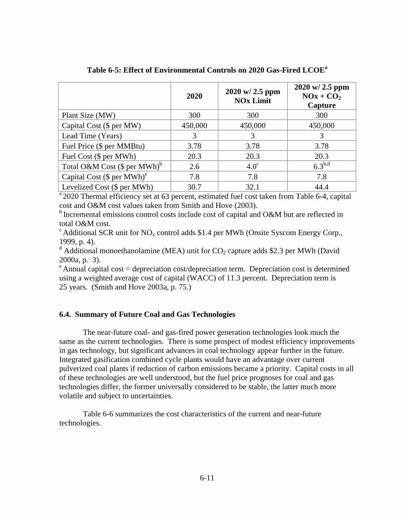
6-11

Table 6-5: Effect of Environmental Controls on 2020 Gas-Fired LCOEa

20202020 w/ 2.5 ppm

NOx Limit

2020 w/ 2.5 ppmNOx + CO2

CapturePlant Size (MW) 300 300 300Capital Cost ($ per MW) 450,000 450,000 450,000Lead Time (Years) 3 3 3Fuel Price ($ per MMBtu) 3.78 3.78 3.78Fuel Cost ($ per MWh) 20.3 20.3 20.3Total O&M Cost ($ per MWh)b 2.6 4.0c 6.3b,d

Capital Cost ($ per MWh)e 7.8 7.8 7.8Levelized Cost ($ per MWh) 30.7 32.1 44.4

a 2020 Thermal efficiency set at 63 percent, estimated fuel cost taken from Table 6-4, capitalcost and O&M cost values taken from Smith and Hove (2003).b Incremental emissions control costs include cost of capital and O&M but are reflected intotal O&M cost.c Additional SCR unit for NOx control adds $1.4 per MWh (Onsite Syscom Energy Corp.,1999, p. 4).d Additional monoethanolamine (MEA) unit for CO2 capture adds $2.3 per MWh (David2000a, p. 3).e Annual capital cost = depreciation cost/depreciation term. Depreciation cost is determinedusing a weighted average cost of capital (WACC) of 11.3 percent. Depreciation term is25 years. (Smith and Hove 2003a, p. 75.)

6.4. Summary of Future Coal and Gas Technologies

The near-future coal- and gas-fired power generation technologies look much thesame as the current technologies. There is some prospect of modest efficiency improvementsin gas technology, but significant advances in coal technology appear further in the future.Integrated gasification combined cycle plants would have an advantage over currentpulverized coal plants if reduction of carbon emissions became a priority. Capital costs in allof these technologies are well understood, but the fuel price prognoses for coal and gastechnologies differ, the former universally considered to be stable, the latter much morevolatile and subject to uncertainties.

Table 6-6 summarizes the cost characteristics of the current and near-futuretechnologies.

6-12

Table 6-6: Cost Characteristics of Fossil-Fired Electricity Generation

PulverizedCoal

Combustion

Coal,CirculatingFluidized

Bed

Coal,Integrated

GasificationCombined

Cycle

GasTurbine

CombinedCycle

Capital Cost ($ per kW) 1,189 1,200 1,338 590Fuel Cost ($ per MWh) 11.26 12.04 9.44 23.60Total Operations andMaintenance Cost (O&M) ($ perMWh) 7.73 5.87 5.19 2.60Construction time (years) 4 4 4 3Current Thermal Efficiency(percent) 30 to 35 30 to 35 40 to 45 55 to 60R&D Thermal EfficiencyTargets (percent) 45 45 60 65

Sources: Table 6-1, Table 6-3.

6-13

References

Agrawal R.K., and Wood, S.C. (2001) “Cost-Effective NOx Reduction,” ChemicalEngineering 108: 78-82.

Alvey, J. (2003) “The Carbon Conundrum: Technology Exists to Sequester Carbon – ButWill Utilities Ever Buy It?” Public Utilities Fortnightly August: 20-24.

Basu, A., Wainwright, J. (2001) “DME as a Power Generation Fuel: Performance in GasTurbines.” PETROTECH-2001 Conference, New Delhi, India.

Chase, D.L. (2000) “Combined-Cycle. Development, Evolution and Future.” TechnicalReport GER-4206. GE Power Systems.

Claeson Colpier, U., and D. Cornland. (2002) “Economics of the Combined Cycle GasTurbine – An Experience Curve Analysis,” Energy Policy 30: 309-316.

Corman, J. (1996) “Gas Turbine Combined Cycle.” Report. GE Power Systems.

David, J. and H. Herzog. (2000) “The Cost of Carbon Capture.” Paper presented at the FifthInternational Conference on Greenhouse Gas Control Technologies, Cairns, Australia,August 13 to 16.

Energy Information Administration (EIA). (1997) “The Effects of Title IV of the Clean AirAct Amendments of 1990 on Electric Utilities: An Update.” USDOE/EIA-0582(97).Washington D.C.: EIA, March.

Energy Information Administration (EIA). (2001) “Annual Coal Report 2001.”USDOE/EIA-0584. Washington D.C.: EIA.

Energy Information Administration (EIA). (2002a) “Inventory of Electric Utility PowerPlants in the United States 2000.” USDOE/EIA-0095(2002). Washington D.C.: EIA,March.

Energy Information Administration (EIA). (2002b) “U.S. Coal Supply and Demand: 2002Review.” Washington, D.C.: EIA.

Energy Information Administration (EIA). (2003a) Annual Energy Outlook 2003 WithProjections to 2025. USDOE/EIA-0383(2003). Washington D.C.: EIA, January.

Energy Information Administration (EIA). (2003b) “Electric Power Monthly April 2003.”USDOE/EIA-0226(2003/04). Washington D.C.: EIA.

Franco, A., and C. Casarosa. (2002) “On Some Perspectives for Increasing the Efficiency ofCombined Cycle Power Plants,” Applied Thermal Engineering 22: 1501-1518.

6-14

Gillenwater, M.W. (1996) The Aging Stock of Coal-Fired Electric Generating Units:Utilization, Retirements, Repowering, Additions and Environmental Policy Implications.M.S. Thesis, Cambridge, Mass.: Massachusetts Institute of Technology, May.

Greenspan, A. (2003) “Natural Gas Supply.” Testimony before Senate Committee onEnergy and Natural Resources, Federal Reserve Board. Washington, D.C.

Henning, B. (2002) “Natural Gas and Electricity Generation: Market and OperationalConvergence.” Presentation, NASEO Annual Conference. Energy and EnvironmentalAnalysis, Inc.

Heppenstall, T. (1998) “Advanced Gas Turbine Cycles for Power Generation: A CriticalReview,” Applied Thermal Engineering 18: 837-846.

Herzog, H. (2000) “The Economics of CO2 Separation and Capture,” Technology 7,supplement 1: 13-23.

Herzog, H.J., and D. Golomb. (2004) “Carbon Capture and Storage from Fossil Fuel Use,”forthcoming in C. Cleveland, ed., Encyclopedia of Energy. Amsterdam: Elsevier.

International Energy Agency (IEA). (2000) “Hybrid Plants for Coal and Natural GasFiring,” Profiles, December, pp. 1-2.

Miller, N., and E. Huseyin. (2002) “Liquefied Natural Gas – A Burning Issue,” PowerEconomics, April, pp. 18-20.

National Coal Council. (1998) “Coal’s Role in Achieving Economic Growth andEnvironmental Stability: An Interpretive Report on Recent Global Climate Change Studieswith a Long Range and Strategic Perspective on Enabling Technologies.” Washington, D.C.:National Coal Council, November.

National Coal Council. (1997) “Vision 2020: The Role of Coal in U.S. Energy Strategy.”Washington, D.C.: National Coal Council, February.

National Petroleum Council (NPC). (1999) Meeting the Challenges of the Nation’s GrowingNatural Gas Demand. Retrieved December 2003 from the World Wide Web:http://www.npc.org/reports/ReportVol1.pdf.

Naughten, B. (2003) “Economic Assessment of Combined Cycle Gas Turbines in Australia:Some Effects of Microeconomic Reform and Technological Change,” Energy Policy 31:225-245.

New York Mercantile Exchange (NYMEX). (2003) “Natural Gas Futures Data.” RetrievedAugust 2003 from the World Wide Web: http://www.nymex.com/jsp/markets/ng_fut_csf.jsp

6-15

Northwest Power Planning Council. (2002) Natural Gas Combined Cycle Gas TurbinePower Plants. Retrieved December 2003 from the World Wide Web:http://www.westgov.org/wieb/electric/Transmission%20Protocol/SSG-WI/pnw_5pp_02.pdf.

Onsite Sycom Energy Corporation. (1999) Cost Analysis of NOx Control Alternatives forStationary Gas Turbines. Retrieved December 2003 from the World Wide Web:http://www.eere.energy.gov/der/industrial_turbines/pdfs/noxcntlcost.pdf.

Phillips, J. N. (2000) “Hydrogen-Enriched Natural Gas Offers Economic NOx ReductionAlternative,” Power Engineering 104: 36-39.

Schmoke, James W., and Thaddeus S. Dyman. (2001) Changing Perceptions of U.S.Natural Gas Resources as Shown by Successive Department of Interior Assessments. U.S.Geological Survey Bulletin 2172-B. Washington, D.C.: U.S. Geological Survey.Retrieved December 2003 from the World Wide Web: http://pubs.usgs.gov/bul/b2172-b.

Simmons, Matthew R. (2003) “Future Energy Resources: Are We Asking the RightQuestions?” Presentation to the National Defense University Workshop. Houston:Simmons International, Inc., May 9.

Smith, Richard, and Anders Hove. (2003) “The Old Reliables: Coal, Nuclear and Gas in2003.” New York: Deutsche Bank AG.

Spath, P.L, and M.K. Mann. (2000) Life Cycle Assessment of a Natural Gas Combined-Cycle Power Generation System. Retrieved December 2003 from the World Wide Web:http://bioproducts-bioenergy.gov/pdfs/bcota/abstracts/13/99.pdf.

U.S. Department of Energy (DOE). (1999a) “Clean Coal Technology: The Investment PaysOff.” Washington, D.C.: U.S. Department of Energy, November.

U.S. Department of Energy (DOE). (1999b) “Coal and Power Systems Strategic and Multi-Year Program Plans.” Washington, D.C.: U.S. Department of Energy, January.

U.S. Department of Energy (DOE). (2000) “Coal and Power Systems Strategic and Multi-Year Program Plans: Ensuring Clean, Affordable Power for the 21st Century.” Washington,D.C.: U.S. Department of Energy, March.

U.S. Department of Energy (DOE). (2003) “Draft Environmental Assessment ToxeconRetrofit for Mercury and Multi-Pollutant Control.” USDOE/EA-1476. Washington, D.C.:U.S. Department of Energy, June.

U.S. Environmental Protection Agency (EPA). (2002a) “Technical Addendum:Methodologies for the Benefit Analysis of the Clear Skies Initiative, September 2002,”Washington, D.C.: EPA.

6-16

U.S. Environmental Protection Agency (EPA). (2003) “Initial Results of Updated ClearSkies Analysis, July 2, 2003,” Washington, D.C.: EPA.

U.S. Environmental Protection Agency (EPA). (2002b) “The Clear Skies Act TechnicalSupport Package.” Washington, D.C.: EPA, September.

U.S. Environmental Protection Agency (EPA). (2002c) “Engineering and Economic FactorsAffecting the Installation of Control Technologies for Multipollutant Strategies FinalReport.” EPA-600/R-02/073. Washington, D.C.: EPA, October.

World Coal Institute. (1999) Power for Progress. London, January.

7-1

Chapter 7. FUEL PRICES

Summary

This chapter examines forecasts for the three fuels of concern: coal, natural gas, anduranium. Coal prices in the United States are not expected to increase. Forecasts for naturalgas prices are mixed, although EIA forecasts a 20 to 30 percent increase over 2002 levels by2020. The supply elasticity of uranium is estimated by several sources to be between 2.3 and3.3, which should keep uranium prices down in the near term.

Some uncertainty surrounds projections of fuel price changes, which can alter relativecompetitiveness between gas and coal, and can also affect competitiveness of both withnuclear. This chapter sums up the significant similarities and differences in the underlyingmethodologies of the various models for coal, natural gas, and uranium supply.

Coal supplies worldwide are expected to be sufficiently elastic that even a doublingof demand is not expected to increase price appreciably. Much of the work on coal prices isshort-term in nature and hence is of limited usefulness for the projections needed for thepresent study. Long-term changes in past decades that have affected coal prices haveincluded dramatic increases in coal mining efficiency, the past trajectory of which may be ofsome help in predicting the future. Among the model forecasts, there is general agreementthat coal production will increase over the next 20 to 30 years (35 to 50 percent). Theinternational forecasts foresee a rise in the international coal price (25 to 30 percent), whilethe forecasts for the U.S. coal price to utilities uniformly predict a decline (10 percent).

EIA’s 2003 gas price predictions are for a 10 percent dip from the 2003 level,followed by a 38 percent increase by 2025. Its 2003 supply prediction is for a relativelysmooth 34 percent increase over the 2003 level by 2025, reduced in the 2004 prediction to15 percent. EIA’s 2004 forecast projects less of a price dip in 2005, followed by a larger riserelative to 2000 levels by 2025.

The International Energy Agency (IEA) and EIA have uranium market models, butthey are limited. The International Atomic Energy Agency (IAEA) offers an outlook onpotential uranium market trends, but it does not incorporate a model of investment inexploration. Since the fuel cost share of nuclear power generation is less than 10 percent,variation in uranium prices will have only a limited effect on the overall cost of nucleargeneration of electricity.

7-2

Outline

7.1. Introduction

7.2. Coal

7.2.1. The Forecasting Models: NEMS, POLES, and WEM7.2.2. Coal Price Projections

7.3. Natural Gas

7.3.1. National Energy Modeling System (NEMS)7.3.2. Prospective Outlook on Long-Term Energy Systems (POLES)7.3.3. World Energy Model (WEM)7.3.4. Current Issues in Natural Gas Supply7.3.5. Summary of the Projections

7.4. Uranium

7.4.1. International Atomic Energy Agency’s Analysis of Uranium Supply to 2050

7.4.2. International Energy Agency’s “Global Uranium Supply Outlook”7.4.3. Estimates of Uranium Supply Elasticity7.4.4. Uranium Market Model of the U.S. DOE7.4.5. Effects of Uranium Price on Cost of Nuclear Power Generation

7.5. Other Models

7.5.1. Energy and Power Evaluation Program7.5.2. Model for Energy Supply Strategy Alternatives and their General

Environmental Impact (MESSAGE)

7.6. Conclusion

7.6.1. Coal7.6.2. Natural Gas7.6.3. Uranium

References

7-3

7.1. Introduction

This chapter reviews and evaluates fuel price forecasts to be used in the analysis ofnuclear power’s competitiveness with coal and gas. The chapter examines major modelingsystems of coal, natural gas, and uranium supply currently in use by government andinternational agencies, focusing on their supply functions for these fuels and thesophistication of the price forecasts.

A focus on current levels of known reserves of a resource, in terms of a certainnumber of years’ consumption remaining, can prompt alarm at the prospect of running out ofa critical mineral such as natural gas from North America. Short-term price fluctuationsextrapolated to the future can yield intermediate-term forecasts that could cause majorchanges in the electricity sector were they to materialize.

Sections 7.2, 7.3, and 7.4 review models of coal, natural gas, and uranium supply.Models of oil supply are excluded from this analysis since the use of oil for electricitygeneration is not widespread in the United States. Section 7.5 examines modeling systemsthat deal with the fuels in a generic manner. Section 7.6 summarizes the price and supplyprojections.

7.2. Coal

Three economic models of coal are reviewed in this section, the EIA’s NationalEnergy Modeling System (NEMS), the European Union’s Prospective Outlook on Long-Term Energy Systems (POLES), and the International Energy Agency’s World EnergyModel (WEM).

7.2.1. The Forecasting Models: NEMS, POLES, and WEM

NEMS and POLES include different specifications to forecast coal production andprices. The Coal Production Submodule (CPS) of NEMS is responsible for the constructionof annual supply curves for each combination of region, mine type, and coal type found inthe United States. Using two-stage least squares regression methodology, a supply functionis created that relates price to mine capacity utilization (EIA 2003c, p.8). It is then calibratedto the most recent data (EIA 2003c, p.17).

The POLES model evaluates future coal supply from a global perspective. Itestimates production for each of thirty-two national and regional markets. National andregional supplies are modeled as a function of the previous year’s coal production, a short-term price effect, a long-term price effect with a distributed lag and asymmetric responsefactor, coal consumption in the current and previous year, and an autonomous technologicaltrend, differentiating between exporting and non-exporting areas in its supply specifications(Criqui et al. 2003, 2.3). For countries that are large producers or exporters of coal, alsocalled swing producers, which includes the United States, POLES models a national coal

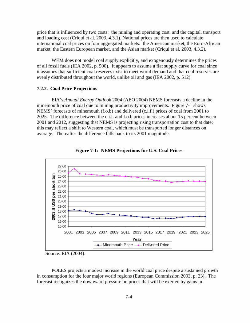
7-4

price that is influenced by two costs: the mining and operating cost, and the capital, transportand loading cost (Criqui et al. 2003, 4.3.1). National prices are then used to calculateinternational coal prices on four aggregated markets: the American market, the Euro-Africanmarket, the Eastern European market, and the Asian market (Criqui et al. 2003, 4.3.2).

WEM does not model coal supply explicitly, and exogenously determines the pricesof all fossil fuels (IEA 2002, p. 500). It appears to assume a flat supply curve for coal sinceit assumes that sufficient coal reserves exist to meet world demand and that coal reserves areevenly distributed throughout the world, unlike oil and gas (IEA 2002, p. 512).

7.2.2. Coal Price Projections

EIA’s Annual Energy Outlook 2004 (AEO 2004) NEMS forecasts a decline in theminemouth price of coal due to mining productivity improvements. Figure 7-1 showsNEMS’ forecasts of minemouth (f.o.b) and delivered (c.i.f.) prices of coal from 2001 to2025. The difference between the c.i.f. and f.o.b prices increases about 15 percent between2001 and 2012, suggesting that NEMS is projecting rising transportation cost to that date;this may reflect a shift to Western coal, which must be transported longer distances onaverage. Thereafter the difference falls back to its 2001 magnitude.

Figure 7-1: NEMS Projections for U.S. Coal Prices

15.00

16.00

17.00

18.00

19.00

20.00

21.00

22.00

23.00

24.00

25.00

26.00

27.00

2001 2003 2005 2007 2009 2011 2013 2015 2017 2019 2021 2023 2025

Year

2003

:II

US

$ p

er s

ho

rt t

on

Minemouth Price Delivered Price

Source: EIA (2004).

POLES projects a modest increase in the world coal price despite a sustained growthin consumption for the four major world regions (European Commission 2003, p. 23). Theforecast recognizes the downward pressure on prices that will be exerted by gains in

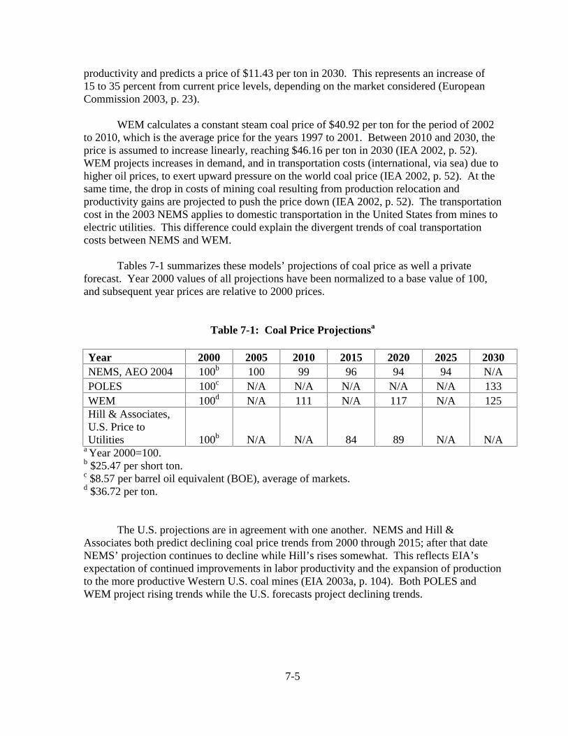
7-5

productivity and predicts a price of $11.43 per ton in 2030. This represents an increase of15 to 35 percent from current price levels, depending on the market considered (EuropeanCommission 2003, p. 23).

WEM calculates a constant steam coal price of $40.92 per ton for the period of 2002to 2010, which is the average price for the years 1997 to 2001. Between 2010 and 2030, theprice is assumed to increase linearly, reaching $46.16 per ton in 2030 (IEA 2002, p. 52).WEM projects increases in demand, and in transportation costs (international, via sea) due tohigher oil prices, to exert upward pressure on the world coal price (IEA 2002, p. 52). At thesame time, the drop in costs of mining coal resulting from production relocation andproductivity gains are projected to push the price down (IEA 2002, p. 52). The transportationcost in the 2003 NEMS applies to domestic transportation in the United States from mines toelectric utilities. This difference could explain the divergent trends of coal transportationcosts between NEMS and WEM.

Tables 7-1 summarizes these models’ projections of coal price as well a privateforecast. Year 2000 values of all projections have been normalized to a base value of 100,and subsequent year prices are relative to 2000 prices.

Table 7-1: Coal Price Projectionsa

Year 2000 2005 2010 2015 2020 2025 2030NEMS, AEO 2004 100b 100 99 96 94 94 N/APOLES 100c N/A N/A N/A N/A N/A 133WEM 100d N/A 111 N/A 117 N/A 125Hill & Associates,U.S. Price toUtilities 100b N/A N/A 84 89 N/A N/A

a Year 2000=100.b $25.47 per short ton.c $8.57 per barrel oil equivalent (BOE), average of markets.d $36.72 per ton.

The U.S. projections are in agreement with one another. NEMS and Hill &Associates both predict declining coal price trends from 2000 through 2015; after that dateNEMS’ projection continues to decline while Hill’s rises somewhat. This reflects EIA’sexpectation of continued improvements in labor productivity and the expansion of productionto the more productive Western U.S. coal mines (EIA 2003a, p. 104). Both POLES andWEM project rising trends while the U.S. forecasts project declining trends.

7-6

7.3. Natural Gas

Natural gas forecasts are made with NEMS, POLES, and WEM.

7.3.1. National Energy Modeling System (NEMS)

NEMS’s treatment of natural gas supply is sophisticated in its reserve-production-price interactions and comprehensive in its resource coverage (EIA 2003e). Based onMacAvoy and Pindyck (1974, Chapter 3), NEMS’s natural gas model incorporatesinvestment in exploration as a function of expected profitability, which depends in turn onexisting reserves and the current ratio of production to reserves. The success of explorationin finding new reserves is estimated econometrically from historical data, and newlydiscovered fields infer additional reserves that require additional drilling before they can bedeclared proven. The supply and wellhead price projections are derived by solving twoequations, one relating production from existing wells to recent price changes, the otherrelating wellhead price in the current year to the previous year’s expected price, expected andactual production, and the oil price. A supply curve for gas is generated from the solution tothis equation.

NEMS projects gas production from unconventional deposits, including coalbedmethane, tight gas sands, and gas shales, estimating economic feasibility of recovery on thebasis of their locations, resource quantity and quality, and technology. Arctic gas is modeledon the basis of discrete projects, each requiring pipeline construction, using discounted cashflow to assess the profitability of the pipeline.

Liquified Natural Gas (LNG) imports are treated with a foreign natural gas supplysubmodule. LNG competes with CIF (the cost including insurance and freight) domestic gasprice in the vicinity of a terminal rather than with the free-on-board (FOB) wellhead price.

NEMS forecasts the average Lower 48 natural gas wellhead price to increase steadilyfrom around 2005 through 2025, following a dip after the early 2000s spike. Figure 7-2shows the reference case trend. Depletion of North American gas resources is cited as theprimary factor driving the increase in the wellhead price (EIA 2003a, p. 75). The productionforecast of AEO 2003 is for a 34 percent increase over the 2000 level by 2025, but the AEO2004 forecast lowers that to a 15 percent increase.

7-7

Figure 7-2: U.S. Lower 48 Average Natural Gas Wellhead Price

2

3

4

5

6

2001 2003 2005 2007 2009 2011 2013 2015 2017 2019 2021 2023 2025

Year

200

3:II

US

$/1

00

0 c

u. f

t.

Source: EIA (2004).

Figure 7-3 shows NEMS’ forecast errors of gas prices from two years’ forecasts.Only 7 years are available to compare forecasting performance, but the 1995 forecast may besuperior to the 1989 forecast since it cycles around zero instead of trending off, although theyare predicting for different calendar years. It seems that NEMS’ gas price forecasts, even ifthey are off by 25 percent, are improving with experience.

Figure 7-3: Natural Gas Wellhead Price: Difference between Actual and Forecast

Source: Holte (2001, Table 8).

-50

-25

0

25

50

75

100

125

150

175

0 2 4 6 8 10 12Years into future

per

cen

t d

iffe

ren

ce

Years Ahead From 1989 Years Ahead From 1995

7-8

As with coal, it is evident that EIA has not been entirely successful in its forecasts ofnatural gas prices. There is also evidence of learning in the forecasting methodology, as the1995 forecasts perform better than the 1989 forecasts. Natural gas was the last fuel to beaffected by regulatory reforms following the period of more extensive controls on energymarkets in the 1970s and early 1980s, and the trends of natural gas prices and production incompetitive markets have not been stable. In earlier projections, the natural gas outlook wasstrongly influenced by the world oil price forecast, which was subject to its own error.Beyond market factors, transient external factors such as severe weather are not anticipatedby the forecasting models (Holte 2001).

7.3.2. Prospective Outlook on Long-Term Energy Systems (POLES)

Like the POLES model for coal supply, the POLES gas supply model simulatesproduction in national modules, then adjusts the production of the swing producers accordingto international market interactions. Prices are determined for three markets—American,European, and Asian. The national modules incorporate a discovery-process model for gassupply, but specific drilling effort for gas is not modeled. Gas discoveries are limited byultimate recoverable resources of gas, but are modeled as a function of the drilling effort foroil rather than by direct modeling of gas exploration. POLES makes this simplificationpartly because of lack of data but primarily because “oil companies look for oil and manytime[s] find gas” (Criqui et al. 2003, 2.2).

The European Commission’s “World Energy, Technology, and Climate PolicyOutlook” (WETO) uses POLES to predict gas prices on three continental markets, America,Europe/Africa, and Asia. In the European/African market, the price is forecasted to risesteadily to $32 per barrel (bbl.) in 2030. In the American market, prices first decline fromthe high level of 2000 down to $16 per bbl. by 2010, and then rise steadily to $29 per bbl. in2030. In the Asian market, prices rise from $23 per bbl. in 2001 to $38 per bbl. in 2030. Thedifferences between the three regional prices are attributable in part to the mix of pipeline gasand LNG but more generally reflect the low degree of integration of gas markets acrossworld regions, as found in Chapter 9. The price differentials are expected to “diminishsignificantly” over the forecasting horizon as the gas supply mixes become more similar(European Commission 2003, p. 21).

The rapid growth in natural gas reserves observed in the past is expected to continuefor the next decade, followed by a moderate decrease (European Commission 2003, p. 42).WETO predicts that interregional gas trade would represent roughly 36 percent of worldwidegas consumption in 2030, compared to 14 percent currently. This increase in the gas trade“will imply new investments in long distance pipelines from producing to consuming regionsand significantly increased LNG trade and investments in LNG infrastructure” (EuropeanCommission 2003, p. 90).

7-9

7.3.3. World Energy Model (WEM)

The gas supply module in WEM estimates production field by field to determineshort-term production profiles, while in the long term production is limited by ultimatelyrecoverable resources and a depletion rate estimated through historical data. Ultimatelyrecoverable resources depend on a recovery factor, which reflects technologicalimprovements in drilling, exploration, and production. The trend in the recovery rate is afunction of the gas price, which is set exogenously, and a technological improvement factor(IEA 2002, pp. 510-511).

WEM considers three regional gas markets, North America, Europe, and Asia. InNorth America, natural gas prices are projected to average around $2.62 per MMBtu in 2002and to remain at that level until 2005. Prices will then start to rise as rising demand causesthe region to become increasingly reliant on more costly sources, such as LNG,unconventional gas, and Alaskan gas (IEA 2002, p. 50). Prices reach $3.15 per MMBtu by2010 and continue to rise in line with oil prices (IEA 2002, p. 50). IEA’s 2002 World EnergyOutlook predicts rising import dependence for the OECD North America region. In 2000,this region’s net gas imports amounted to only 1 percent of the total primary gas supply, butby 2030, imports are expected to rise to 26 percent of the total primary gas supply (IEA2002, p. 117).

7.3.4. Current Issues in Natural Gas Supply

The recent increases in natural gas prices have led to divergent opinions on the futureof natural gas in the United States. In one view these price increases represent fundamentalshifts in supply and demand that have long-term implications for the natural gas market andwill only worsen in the future because of dwindling gas reserves (Simmons 2003). Currie(2003) emphasizes longer-term deterioration of gas pipeline and storage infrastructure, post-deregulation, as a major problem facing the gas industry, but in the long-run time period ofthe current study, capital markets will supply that infrastructure.

A recent study by the National Petroleum Council (NPC) also blames the higher gasprices in recent years on a fundamental shift in the supply-demand balance (NPC 2003, p.23). However, the NPC believes the tight market situation “can be moderated” (NPC 2003,p. 23) by allowing exploration and production in currently restricted areas offshore and in theRocky Mountains, using new technologies that can protect sensitive environmental resources(NPC 2003, pp. 76-77).

7.3.5. Summary of Gas Price Projections

Table 7-2 reports NEMS, POLES, and WEM projections of natural gas prices through2020, and two private forecasts reported by the AEO 2003, those of Global Insights, Inc.(GII) and Energy Ventures Analysis, Inc. (EVA). The NEMS forecasts from the AEO 2003and AEO 2004 are reported in the first two rows of the table, showing a sharp increase inEIA’s gas price forecast between these two years. Prices are expressed relative to a base of

7-10

2000 prices set to 100. NEMS and POLES agree on the dip between 2000 and 2005 andsubsequent rise through 2020. WEM and the two private forecasts do not report near-termforecasts but agree on a rising trend by 2010, from a level below 2000 prices.

Table 7-2: Natural Gas Price Projectionsa

Year 2000 2005 2010 2015 2020NEMS Lower 48 U.S .Wellhead Price,AEO 2003 100b 75 86 93 96NEMS Lower 48 U.S. Wellhead Price,AEO 2004 100b 92 88 109 111

POLES, American Market Price 100c 69 73 81 94

WEM North American Market Price 100d N/A 69 N/A 87GII Lower 48 U.S. Wellhead Price 100b N/A N/A 82 84EVA Lower 48 U.S. Wellhead Price 100b N/A N/A 99 81

aYear 2000=100.b$3.93 per 1000 cu. ft.c$21.95 per BOE (bbl oil equivalent).d$4.09 per MMBtu.

7.4. Uranium

7.4.1. International Atomic Energy Agency’s Analysis of Uranium Supply to 2050

Due to the long time spans involved in the life cycles of uranium mines and nuclearpower plants, projections for uranium require a longer forecasting horizon compared to otherfuels (IAEA 2001, foreword). In its projections of global uranium production, theInternational Atomic Energy Agency (IAEA) considers three uranium demand cases (low,middle, and high) covering a range of assumptions regarding global economic growth andnuclear energy policy. In the low demand case, economic growth is of medium pace, withenergy demand growth consequently low. In this case, energy policies are ecologicallydriven, and nuclear power is phased out by 2100. The medium demand case is alsocharacterized by medium economic growth, low energy demand growth, and ecologicallydriven energy policies, but the entire world, including developing countries, sees a sustaineddevelopment of nuclear power. The high demand case foresees high economic growth and a“rich and clean” energy future without recourse to strict environmental policies. Nuclearpower develops significantly in the high demand case (IAEA 2001, p. 1).

The main focus of the IAEA analysis is to assess the adequacy of conventionaluranium resources to satisfy market-based production requirements. Conventional resourcesare defined as those that have an established history of production where uranium is either aprimary product, co-product, or important by-product (e.g., gold). Such resources are

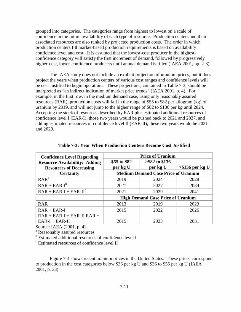
7-11

grouped into categories. The categories range from highest to lowest on a scale ofconfidence in the future availability of each type of resource. Production centers and theirassociated resources are also ranked by projected production costs. The order in whichproduction centers fill market-based production requirements is based on availabilityconfidence level and cost. It is assumed that the lowest-cost producer in the highest-confidence category will satisfy the first increment of demand, followed by progressivelyhigher-cost, lower-confidence producers until annual demand is filled (IAEA 2001, pp. 2-3).

The IAEA study does not include an explicit projection of uranium prices, but it doesproject the years when production centers of various cost ranges and confidence levels willbe cost-justified to begin operations. These projections, contained in Table 7-3, should beinterpreted as “an indirect indication of market price trends” (IAEA 2001, p. 4). Forexample, in the first row, in the medium demand case, using only reasonably assuredresources (RAR), production costs will fall in the range of $55 to $82 per kilogram (kg) ofuranium by 2019, and will not jump to the higher range of $82 to $136 per kg until 2024.Accepting the stock of resources described by RAR plus estimated additional resources ofconfidence level I (EAR-I), those two years would be pushed back to 2021 and 2027, andadding estimated resources of confidence level II (EAR-II), these two years would be 2021and 2029.

Table 7-3: Year When Production Centers Become Cost Justified

Price of Uranium$55 to $82per kg U

>$82 to $136per kg U >$136 per kg U

Confidence Level RegardingResource Availability: Adding

Resources of DecreasingCertainty Medium Demand Case Price of Uranium

RARa 2019 2024 2028RAR + EAR-Ib 2021 2027 2034RAR + EAR-I + EAR-IIc 2021 2029 2041

High Demand Case Price of UraniumRAR 2013 2019 2023RAR + EAR-I 2015 2022 2026RAR + EAR-I + EAR-II RAR +EAR-I + EAR-II 2015 2023 2031

Source: IAEA (2001, p. 4).a Reasonably assured resourcesb Estimated additional resources of confidence level Ic Estimated resources of confidence level II

Figure 7-4 shows recent uranium prices in the United States. These prices correspondto production in the cost categories below $36 per kg U and $36 to $55 per kg U (IAEA2001, p. 33).

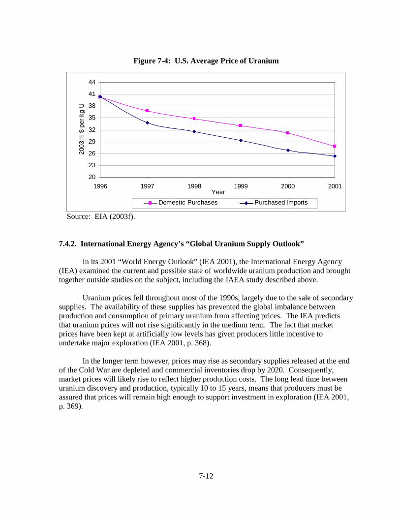
7-12

Figure 7-4: U.S. Average Price of Uranium

20

23

26

29

32

35

38

41

44

1996 1997 1998 1999 2000 2001Year

2003

:II

$ pe

r kg

U

Domestic Purchases Purchased Imports

Source: EIA (2003f).

7.4.2. International Energy Agency’s “Global Uranium Supply Outlook”

In its 2001 “World Energy Outlook” (IEA 2001), the International Energy Agency(IEA) examined the current and possible state of worldwide uranium production and broughttogether outside studies on the subject, including the IAEA study described above.

Uranium prices fell throughout most of the 1990s, largely due to the sale of secondarysupplies. The availability of these supplies has prevented the global imbalance betweenproduction and consumption of primary uranium from affecting prices. The IEA predictsthat uranium prices will not rise significantly in the medium term. The fact that marketprices have been kept at artificially low levels has given producers little incentive toundertake major exploration (IEA 2001, p. 368).

In the longer term however, prices may rise as secondary supplies released at the endof the Cold War are depleted and commercial inventories drop by 2020. Consequently,market prices will likely rise to reflect higher production costs. The long lead time betweenuranium discovery and production, typically 10 to 15 years, means that producers must beassured that prices will remain high enough to support investment in exploration (IEA 2001,p. 369).

7-13

7.4.3. Estimates of Uranium Supply Elasticity

Low prices and the availability of large, known uranium reserves have stifledincentives to invest in exploration for new uranium resources for some years. However, ifprice rose enough to stimulate substantial investments in exploration, new uranium resourcesfar larger than today’s resource estimates are likely to be found, according to Bunn et al.(2003, p. 106). Three studies have attempted to estimate the price elasticity of supply foruranium. Bunn et al. developed an empirical relationship relating uranium supply to price,based on a supply curve, R = 2.1(p/ 40)E. They used quantity and price estimates from threeother studies to estimate the magnitude of the elasticity, E. Table 7-4 summarizes theirelasticity estimates. The table also includes the resources projected at particular prices underthe different elasticity estimates.

Table 7-4: Estimates of Uranium Resources

Source E R(MtU)p≤ $84 per kgU

R(MtU)p≤$136 per kgU

Uranium Information Centre 3.32 21 105Deffeyes and MacGregor 2.48 12 40DOE Office of Nuclear Energy 2.35 11 34

Source: Bunn et al. (2003, p. 113).

Although these estimates are based on limited data, Bunn et al. suggest that the totalamount of uranium recoverable at or below $136 per kgU is considerably larger than theamount reported in 2001 by IAEA, anywhere from two to six times larger. They note thatthe relationships resulting in smaller resource estimates are based solely on geologicalrelationships, without considering the likelihood that technology for recovering uranium atlower cost will improve in the future. They claim that technological improvement is“virtually certain,” providing the example that uranium is now recoverable at less than $55per kgU from ores in copper mines with concentrations as low as 4.5 parts per million (Bunnet al. 2003, p. 113).

7.4.4. Uranium Market Model of the U.S. DOE

The Uranium Market Model (UMM), last revised in 1996, is a microeconomicsimulation model that matches uranium supplied by the mining and milling industry with thedemand for uranium by electric utilities operating nuclear power plants (Das and Lee 1996).The model considers every production center and utility worldwide, as well as holders ofstockpiled uranium and other suppliers. The model makes annual projections for 10 globalregions, one of which is the United States.

7-14

The UMM represents uranium supply with an annual short-run supply curve thatrelates increments of potential production to the market price. Supplies come fromproduction and releases from official stockpiles and private inventories. Production costs areexogenous but take into account the size of reserves, annual production capacity, ore grade,and type of production process.

The demand for uranium by electric utilities with nuclear power plants is derivedexogenously. Individual reactor requirements are summed into utility-specific or regionaltotals. Reactor requirements are inelastic with respect to uranium prices, but utilities’inventory demand responds to uranium spot prices.

7.4.5. Effects of Uranium Price on Cost of Nuclear Power Generation

The fuel cost share nuclear power’s busbar cost is small, around 10 percent (Papay1997, Paulson 2002). Moreover, the uranium cost share of the total fuel cost is about10 percent (NEA 1994). Thus, it is unlikely that changes in uranium price of foreseeablemagnitude would materially affect the cost of nuclear power generation.

7.5. Other Models

The models reported in the fuel-specific sections above developed distinct models forcoal and natural gas. Two energy models, Argonne National Laboratory’s and theInternational Institute for Applied Systems Analysis’(IIASA) models, offer fuel forecastswith specifications that are not specifically tailored to individual fuels.

7.5.1. Energy and Power Evaluation Program

The Energy and Power Evaluation Program (ENPEP) was developed at ArgonneNational Laboratory and is distributed by Adica Consulting, LLC. ENPEP simulates energymarkets and determines supply/demand balances over a long-term period of up to 75 years.The BALANCE module of ENPEP models a national energy network consisting of energyactivities from production to final utilization, each called a node. The nodes are connectedby links, which convey price and quantity information between nodes (Adica 2002, pp. 1-3).

The Depletable Resource Node models the production of a depletable resource, suchas coal, natural gas, or crude oil, which can be domestically produced or imported. Theequation associated with this node relates the cost of producing or importing increments of agiven resource to the cumulative amount of the resource produced or imported. Thisequation represents ENPEP’s long-run supply curve for the resource (Adica 2002, p. 5).

7-15

7.5.2. Model for Energy Supply Strategy Alternatives and their General EnvironmentalImpact (MESSAGE)

7.5.2.1. The Model

The Model for Energy Supply Strategy Alternatives and their General EnvironmentalImpact (MESSAGE) was developed by IIASA. MESSAGE models fuel supply throughdetailed domestic resource extraction constraints and elasticity definitions, in addition toconstraints on imports and exports.

MESSAGE calculates a supply elasticity as the change in price relative to a referenceprice level that results from a change in supply over a reference supply level (Messner andStrubegger 2001, p. 47). The model contains an equation that balances production andimport of primary energy with central conversion, transport, and export requirements(Messner and Strubegger 2001, p. 28). This equation takes into account the level oftechnology involved in the extraction a given resource (Messner and Strubegger 2001, p. 29).

MESSAGE was used for the projections in Global Energy Perspectives, publishedjointly by IIASA and the World Energy Council (WEC) in 1998. Although this publicationdoes not include projections of fuel prices, it does include projections of fuel production byregion. The projections for North American (U.S. and Canadian) gas production under sixdifferent scenarios are shown in Table 7-5. The timing and extent of new discoveries ofreserves and resources are incorporated as assumptions in the scenarios (IIASA and WEC1998, p. xiii). The numbers indicate that the scenarios represent distinctly different futures,even within a period of only three decades.

All the scenarios in MESSAGE project increasing North American natural gasproduction from 2000 through 2020, although scenarios B, C1 and C2 see production fallingoff from 2010 to 2020.

Table 7-5: MESSAGE Forecasts of North American Gas Production

North America Natural Gas Production (Mtoe)Scenario 2000 2010 2020A1: high growth, ample oil and gas 587 727 806A2: high growth, return to coal 580 716 734A3: high growth, fossil phaseout 620 794 997B: middle course 583 712 690C1: ecologically driven, new renewableswith nuclear phaseout 506 569 545C2: renewables and new nuclear 507 593 562

7-16

7.6. Conclusion

The models examined in this report differ in the scopes of their projections. The coaland gas models account for feedbacks between proven reserve base, price, and exploration,but the uranium models remain more rudimentary in their characterizations of supply.

The projections of NEMS focus on future energy trends in the United States, whilePOLES, WEM, and MESSAGE have a more international orientation. This sectionsummarizes some of the important similarities and differences in the underlyingmethodologies of the various models for coal, natural gas, and uranium supply andrecapitulates their projected trends.

7.6.1. Coal

NEMS’ coal supply modeling is the most sophisticated among the three modelsexamined. The U.S. forecasts, from NEMS and Hill & Associates, agree on a declining coalc.i.f. (cost including insurance and freight) price forecast from 2000 through 2020 of about10 percent, but POLES and WEM both predict rising international coal prices, as much as25 to 30 percent. All the models agree that coal production will increase 35 to 50 percentover the next 20 to 30 years.

7.6.2. Natural Gas

As with coal supply models, NEMS provides the most comprehensive model of gassupply. Gas prices are projected to fall after the initial spikes, a pattern replicated across themodels. Production is projected to increase over the forecast horizon by 15 to 40 percent,across models and scenarios.

7.6.3. Uranium

While IAEA offers an outlook on potential uranium market trends, it does notincorporate a model of investment in exploration. It warns that exploration needs to occur toensure a low-cost supply of uranium but does not model factors influencing it. Unlike thenatural gas models, none of the uranium modeling take into account the determinants anduncertainties of exploration, possibly because there has been relatively little recentexploration for uranium. Unique factors are at play in uranium exploration, chiefly the longlead time between discovery and production. The major issue in the future of uranium is thecost at which future exploration might allow supplies to be produced.

7-17

References

Adica Consulting, LLC. (2002) “Description of the ENPEP Model.” Retrieved September10, 2003 from the World Wide Web:http://www.adica.com/main/media/demos/ENPEP_summary.pdf.

Bunn, Matthew, Steve Fetter, John P. Holdren, and Bob van der Zwaan. (2003) “TheEconomics of Reprocessing vs. Direct Disposal of Spent Nuclear Fuel.” Cambridge, Mass.:President and Fellows of Harvard University.

Criqui, Patrick, Silvana Mima, and A. Tuan Nguyen. (2003) “POLES 4: ProspectiveOutlook on Long-term Energy Systems.” Grenoble, France: Institute of Economy andEnergy Policy.

Currie, Jeffrey R. (2003) “Natural Gas Supply and Demand Issues.” Testimonybefore the Full Committee on Energy and Commerce, U.S. House of Representatives,Washington, D.C. New York: Goldman, Sachs & Co., June 10.

Das, Sujit, and Russell Lee. (1996) “Model Documentation of the Uranium MarketModel (UMM).” Washington, D.C.: Energy Information Administration.

Deffeyes, Kenneth, and Ian D. MacGregor. (1980) “World Uranium Resources,”Scientific American 242, No. 1: 50-60.

Energy Information Administration (EIA). (2003a) Annual Energy Outlook 2003with Projection to 2025. Washington D.C.: Energy Information Administration.Supplemental Tables retrieved from the World Wide Web December 2003:http://www.eia.doe.gov/oiaf/archive/aeo2003/supplement/sup_ogc.pdf.

Energy Information Administration (EIA). (2003b) Assumptions for the AnnualEnergy Outlook 2003 with Projection to 2025. Washington D.C.: Energy InformationAdministration.

Energy Information Administration (EIA). (2003c) “Model Documentation: CoalMarket Module.” Washington, D.C.: Energy Information Administration.

Energy Information Administration (EIA). (2003d) “Model Documentation: NaturalGas Transmission and Distribution Module.” Washington, D.C.: Energy InformationAdministration.

Energy Information Administration (EIA). (2003e) “Oil and Gas Supply ModuleDocumentation.” Washington, D.C.: Energy Information Administration.

7-18

Energy Information Administration (EIA). (2003f) “Uranium Overview, 1949-2002.” Washington, D.C.: Energy Information Administration. Retrieved November 20,2003 from the World Wide Web: http://www.eia.doe.gov/emeu/aer/txt/ptb0903.html.

Energy Information Administration (EIA). (2004) Annual Energy Outlook 2004 withProjection to 2025. Washington D.C.: Energy Information Administration, January.Supplemental tables retrieved from the World Wide Web January 2004:http://www.eia.doe.gov/oiaf/aoe/excel/aeo_base.xls

European Commission. (2003) “World Energy, Technology, and Climate PolicyOutlook.” Luxembourg: European Commission.

Holte, Susan H. (2001) “Annual Energy Outlook Forecast Evaluation.” Washington,D.C.: Energy Information Administration. Retrieved September 11, 2003 from the WorldWide Web: http://www.eia.doe.gov/oiaf/archive/analysispaper01/forecast_eval.html.

International Atomic Energy Agency (IAEA). (2001) “Analysis of Uranium Supply to2050.” Vienna: IAEA.

International Energy Agency (IEA). (2001) “World Energy Outlook: Assessing Today’sSupplies to Fuel Tomorrow’s Growth.” Paris: Organization for Economic Co-operation andDevelopment/International Energy Agency.

International Energy Agency (IEA). (2002) World Energy Outlook. Paris: Organization forEconomic Co-operation and Development/International Energy Agency.

International Institute for Applied Systems Analysis and World Energy Council (IIASA &WEC). (1998) Global Energy Perspectives. Cambridge: Cambridge University Press.

MacAvoy, Paul W., and Robert S. Pindyck. (1974) The Economics of the Natural GasShortage (1960-1980). Mimeo. Cambridge, Mass.: Massachusetts Institute of TechnologyEnergy Laboratory. [published by North-Holland, 1975]

Messner, S., and M. Strubegger. (2001) “Model MESSAGE: Command Line User Manual,Version 0.18.” Laxenburg, Austria: International Institute for Applied Systems Analysis.

National Petroleum Council (NPC). (2003) “Balancing Natural Gas Policy—Fuelingthe Demand of a Growing Economy.” Washington, D. C.: National Petroleum Council.

Papay, L., L. Trocki, and R. McKinsey. (1997) “Clean Coal Technology Deployment: FromToday into the Next Millennium.” Bechtel Technology and Consulting. San Francisco.

Paulson, Keith. (2002) “Future Commercial Nuclear Expansion in the US.” World NuclearAssociation Annual Symposium 2002. Retrieved December 2003 from the World Wide Webwww.world-nuclear.org/sym/2002/paulson.htm.

7-19

Simmons, Matthew. (2003) “Future Energy Resources: Are We Asking The RightQuestions?” Houston: Simmons & Co. International. Retrieved November 20, 2003 fromthe World Wide Web:http://www.simmonscointl.com/files/Natl%20Defense%20Univ%20(B&W).pdf.

7-20

8-1

Chapter 8. ENVIRONMENTAL POLICIES

Summary

The future costs per MWh of the major competitors to nuclear energy, not just thepresent costs, need to be considered. In addition to process technology advances andpossible fuel price changes that could reduce coal- and gas-fired costs, environmentalconsiderations could serve to raise the cost of these competitor sources in view of theirsignificance as a source of air pollution. This chapter assesses the potential magnitudes ofthese cost increases on coal- and gas-generated electricity.

In view of global climate concerns, an important emission that remains largelyuncontrolled but could be subject to controls in the future is carbon. Carbon emissions canbe reduced only by thermal efficiency improvements, which have rather tight limits. Captureand sequestration therefore are the longer-term environmental control possibilities forcarbon.

Despite a recent application of capture and sequestration in a gas-fired plant inNorway and an innovative example of sale and re-use between a gas-fired utility in NorthDakota and an oil company in Canada, the technology and likely costs of carbonsequestration are in pre-commercial stages.

While the technologies of carbon capture, transport, injection, and sequestrationcannot be said to be commercialized yet, some cost estimates are available. On a per-megawatt hour basis, assuming 100 km transportation by pipeline, a summary is:

$36 to $65 per MWh for pulverized coal combustion (PCC), including anenergy penalty of 16 to 34 percent

$17 to $29 per MWh for gas turbine combined cycle (GTCC), includingan energy penalty of 10 to 16 percent

$20 to $44 per MWh for integrated gasification combined cycle (IGCC),including an energy penalty of 6 to 21 percent.

An alternative measurement of the future costs of carbon control is through the use ofpermit markets similar to those used by the Acid Rain Program and Federal NOX Budget.Prices generated through permit market trading are interpreted as the approximate future costof reducing present emissions. Thus the prices can be used to estimate the mean cost ofmeeting current emissions standards on a per MWh basis. Partly because of the present lackof a carbon emission standard, the results of models estimating the future price of potentialgreenhouse gas permits that have been reviewed have varied greatly. A carbon price range($50 to $250 per metric ton) has been used to construct upper and lower bounds to theelectricity cost impact. For coal, the cost impact is likely to be between $15 and $75 per

8-2

MWh, and for gas, it is between $10 and $50 per MWh. Significant uncertainty exists inthese estimates due to uncertainty in the amount of carbon that is likely to be controlled.

8-3

Outline

8.1. Introduction

8.2. Present Situation and Future Projections

8.3. Carbon Sequestration Technology and Costs

8.3.1. Separation and Capture8.3.2. Cost Estimates8.3.3. Transport and Injection8.3.4. Summary of Carbon Mitigation Costs

8.4. Carbon Tax and Emissions Permit Trading

8.4.1. Review of Carbon Price Estimates8.4.2. Estimated Effect of Carbon Control

8.5. The Effect of Tradable Emission Permit Programs on Electricity Prices

8.5.1. The SO2 Case8.5.2. The NOX Budget Program8.5.3. Conclusion

References

8-4

8.1. Introduction

This chapter examines the future environmental costs of fossil fuel energy,particularly coal-fired and natural gas-fired electricity. The costs and benefits of current andpotential future technologies for the mitigation of carbon dioxide (CO2), sulfur dioxide (SO2),nitrogen oxides (NOX), and particulate matter (PM) are discussed.

Section 8.2 examines the present and projected future emissions from electricitygeneration in the United States, focusing on criteria pollutants associated with fossil powergeneration. Section 8.3 discusses the current state of carbon sequestration technology andinvestigates the impacts that legislation regarding carbon emissions may have on the futureof fossil fuel-fired power plants. Section 8.4 discusses the potential effects of a carbon taxand emissions permit trading. Section 8.5 discusses the effect of current NOX and SO2

emissions trading programs.

8.2. Present Situation and Future Projections

The role of fossil fuels in future electricity generation is projected to increasesignificantly over the next two decades. EIA (2002) projects the share of electricitygenerated from fossil-fuel fired plants to be 80 percent by 2020, up from 69 percent in 1999.

Natural gas-fired and coal-fired power plants are significant contributors to emissionsof many criteria pollutants and carbon dioxide. In 2000, coal-fired electricity generationemitted 2,154 million tons (short tons used throughout this chapter unless otherwise noted) ofcarbon dioxide (CO2), or 14.1 percent of total emissions (EPA 2002a). Coal-fired powerplants emitted 10.7 million tons of sulfur dioxide (SO2) and 4.7 million tons of nitrogenoxides (NOX), or 62 percent and 17.5 percent of total emissions, respectively (EPA 2002a).Emissions from natural gas-fired plants were much lower, both because of lower output fromthese plants and because emission rates for natural gas-fired plants are lower than for coal-fired plants. Electricity produced from natural gas in 2000 emitted 359 million tons of CO2,roughly 2 percent of total CO2 emissions (EPA 2002a). Natural gas-fired electricitygenerators emitted 0.08 million tons of SO2, and 0.5 million tons of NOX, or roughly0.5 percent and 1.9 percent of total emissions, respectively (EPA 2002a).

EIA projections put CO2 emissions from natural gas and coal-fired power plants at3,182 million tons in 2020, with 2,625 million tons of CO2 coming from coal burning plantsand 505 million tons coming from natural gas-fired electricity generators. These amountsrepresent 13 percent and nearly 3 percent of projected CO2 emissions in 2020 from allsources (EIA 2003c). Future emissions of SO2 from coal-fired power plants are capped bythe Clean Air Act Amendments of 1990 (CAAA 1990) at 8.95 million tons. NOX emissionsare projected to be roughly 4.5 million tons in 2020 (EPA 2003c).

8-5

8.3. Carbon Sequestration Technology and Costs

One of the most widely discussed means of reducing CO2 emissions is carbon captureand sequestration. The basic method is to capture CO2 and inject it into secure geologicformations or into the deep ocean for long-term storage. This method holds much promise,and in a 1997 report, the President’s Committee of Advisors on Science and Technology(PCAST) recommended that funding within DOE’s fossil-energy R&D program bereformulated, emphasizing new technologies such as carbon capture and sequestration(PCAST 1997, p. 5).

Two current projects are being studied to better understand the feasibility of this typeof solution in the reduction of global CO2 emissions. These are the Weyburn project inSaskatchewan, Canada and the Sleipner project in the North Sea off the coast of Norway.The motivations behind these two projects differ.

The Weyburn oil field, located in southeastern Saskatchewan, was discovered in1954, containing approximately 1.4 billion barrels of oil. As production rates declined in thefield, CO2 flooding (injection of CO2 into the field to increase production) was used torecover an additional 130 million barrels of oil and permanently sequester approximately15.4 million net tons of CO2 for a total of 19.8 million tons of CO2. CO2 is captured at theGreat Plains Synfuels Plant in North Dakota (coal-fired power plant) and transported in asupercritical state (2,100 pounds per square inch (psi)) via 323-km pipeline to the Weyburnsite. Approximately 2,756 tons of CO2 per day have been injected into the reservoir sinceSeptember 22, 2000 (Brown et al. 2001).

The CO2 sequestered at the North Sea Sleipner gas fields is not the result of burningfossil fuels, but is an impurity that is removed to prepare the gas for market. Formerly, theCO2 was vented to the atmosphere. When Norway instituted a tax on offshore carbonemissions of U.S. $50 per tonne, it became economically viable to capture and sequester theseparated CO2 (the tax was later lowered to $38 per tonne). By avoiding this tax on onemillion tonnes of CO2 annually (3 percent of Norway’s total CO2 emissions), Statoil was ableto recover its investment of $80 million in two years (Adam 2001).

Since, 1996 Statoil has been injecting the separated CO2 into a sandstone layer,known as the Utsira formation, 800 to 1,000 meters below the seabed (IEA 2003). Afterseparation, the CO2 must be compressed to a supercritical state and injected into the rockyreservoir.

A seismic survey done by the British Geological Survey (BGS) in 1999 showed thatthe CO2 injected into the reservoir is likely to remain in place. The potential for storage islarge. One percent of this reservoir would hold three years’ emissions from all the powerplants in Europe (Adam 2001). A BGS report indicated that the North Sea has the potentialto hold all of the CO2 from European power stations for 800 years (800 billion tonnes) (IEA2003). One concern is that the CO2 may begin to compress, rather than dissipate throughoutthe formation, making future injection more difficult (Adam 2001).

8-6

8.3.1. Separation and Capture

According to Herzog, all current commercial CO2 capture is based on chemicalabsorption of CO2 from flue gas using a monoethanolamine (MEA) solvent (Herzog 1999, p.4). The MEA/CO2 solution is sent to a stripper where it is heated, and nearly pure CO2 isreleased and the MEA is recycled (Herzog 1999, p. 5). Herzog notes that the majority ofcosts associated with carbon sequestration are incurred in separation and capture.

8.3.2. Cost Estimates

David (2000) compares several different studies to estimate costs associated with CO2

separation and capture for three types of new (not retrofit) power plants: Integrated GasCombined Cycle (IGCC), Pulverized Coal Combustion (PCC), and Gas Turbine CombinedCycle (GTCC). He adjusts all the studies to a common economic basis to compare costsacross studies. The averages David computed across studies for each plant type are reportedin Table 8-1. The energy penalty is the additional input energy required to separate andcapture the CO2. Additional energy means additional CO2, so the relevant figure is not CO2

captured, but CO2 avoided.

Table 8-1: Average Costs Across Studies: IGCC, PCC, and GTCC (David 2000)a

Plant Type Incremental Cost ofCapture per MWh

Average Cost perTon of CO2 Avoided

Energy Penalty,Percent

IGCC $17.2 $27 6.4 to 21.4PCC $34.8 $52 15.9 to 34.1

GTCC $15.9 $51 9.8 to 16.1aAlthough not specified in David’s reports, this study’s calculations confirm that thesefigures are metric tons, or tonnes. Yearly operating hours = 6,570 hrs per year; capitalcharge rate = 15 percent per year; coal price at lower heating value (LHV) = $1.24 perMMBtu; natural gas price (LHV) = $2.93 per MMBtu (David 2000).

8.3.3. Transport and Injection

Storage of CO2 is feasible in many different locations, including ocean storage—bothat intermediate depths (> 1,500 m) and deep lake injection (> 3,000 m)—depleted gas and oilreservoirs, deep saline aquifers, and unminable coal seams (Ormerod 2002, Davison 2001).Transportation methods are dependent on both the location of the CO2 source and thelocation of the sequestration site. Transportation methods include pipeline, truck, and oceantanker. Costs associated with transportation would also be highly dependent on the distanceand method used, but average costs have been estimated.

Herzog (2004, p. 10) notes that the costs of transportation via pipeline can varygreatly, depending on factors such as terrain and population density. He estimates the costs

8-7

of pipeline transportation of CO2 for a 1,500 MW coal-fired power plant (equivalent to aflow rate of 10 million metric tonnes per year) to be $0.50 per metric tonne per 100 km.Lower flow rates could be as high as $2.00 to $3.50 per metric tonne CO2 per 100 km(Herzog 2004, Figure 5). These figures are more in line with those cited by the IEAGreenhouse Gas R&D Programme of approximately $1 to $3 per tonne CO2 for 100 km(Davison 2001). Herzog’s estimate of truck transportation of CO2 is $6.00 per metric tonneper 100 km. Table 8-2 estimates the costs of transporting CO2 from different plant typesusing the (low) estimates from Herzog (2004) for pipeline transport ($0.50 per metric tonneper 100 km) and (high) truck transport ($6.00 per metric tonne per 100 km). The estimatespresented are based on the following assumptions:

• Energy penalties for plant types are equal to the averages from studiespresented in David (2000), or 14.53 percent, 25.18 percent, and 13.05 percentfor IGCC, PCC, and GTCC plants, respectively, though no energy penalty isincluded for the additional energy required to transport the CO2 by truck;

• Distance from plant to injection site of 500 km (David 2000 notes that allpower plants in the United States are located within 500 km of possiblesequestration sites); and

• Capture rates of 88.2 percent, 86.9 percent, and 88.0 percent for IGCC,PCC, and GTCC plants, respectively (David 2000).

Table 8-2: Ground Transportation Cost Estimates, by Plant Type, $ per MWh

Plant TypePipeline @

$0.50 Per Metric tonne-100km

Truck Transport @$6.00 per Metric tonne-100

kmIGCC 1.9 22.8PCC 2.1 25.7

GTCC 0.9 11.0

The IEA Greenhouse Gas R&D Programme estimated the costs associated with oceantransport of CO2. Ormerod (2002) notes: “Comparable 0.5 m diameter pipelines … costabout $1.6 million per km. Such pipelines have the capacity for 18,000 [tones of CO2 perday]…. The cost of transporting CO2 for 500 km, by such a pipeline, would be around $12/tCO2….” (Ormerod 2002, p. 13). Ormerod also notes the significant advantages a largerdiameter pipe would have, with a 1-m diameter pipe transporting four times as much per day,but costing less than four times the price of the 0.5-m pipe. The IEA Program estimatestransportation by tanker would be around $2 per tonne of CO2, though added to this would bethe costs associated with a CO2 holding tank at the port, the platform, and the vertical pipe, aswell as operating expenses (Ormerod 2002, p.14).

8-8

Two basic options exist for CO2 sequestration, storage in the oceans and undergroundstorage. Three main geological structures are available for permanent or semi-permanentCO2 sequestration: depleted oil or gas reservoirs, deep saline aquifers, and unminable coalbeds. Each option offers different benefits. The IEA Greenhouse Gas R&D Programestimates that depleted oil and gas reservoirs could store 920 Gt (Gigatonnes) of CO2, deepsaline aquifers 400 to 10,000 Gt, and unminable coal beds an additional 15 Gt.

Herzog (1999) estimates injection and storage costs for CO2 to be between $3 and$5.5 per tonne of CO2. Table 8-3 shows the additional costs injection and storage wouldimpose on power generation, by plant type. As with transportation costs, the cost per MWhis highest for PCC plants and lowest for GTCC plants. These differences are due to thevariations by plant type in CO2 produced per kWh of electricity generated. The IEAGreenhouse Gas R&D Program estimates that the cost of storage in depleted oil and gasreservoirs and deep saline formations to be $1 to $3 per tonne CO2 (Davison et al. 2001).

Table 8-3: Injection and Storage Cost Estimates, by Plant Type, $ per MWh

Plant TypeInjection & Storage @$1.00 per tonne-CO2

Injection & Storage @$5.50 per tonne-CO2

IGCC 0.8 4.2PCC 0.9 4.7GTCC 0.4 2.0

8.3.4. Summary of Carbon Mitigation Costs

For any power plant there are costs associated with producing the power. If CO2

emissions become costly, either through a tax on emissions or through costs associated withsequestration, these costs become part of the private cost of producing power. Alternatively,any revenue from the sale of captured CO2 would be subtracted from the costs. These costshave the form:

FX + CCapture + CTransport + CInjection – PSale + TCO2 = FX+CO2,

Where:FX is cost of power production at facility type X = {IGCC, PC, NGCC}) without sequestration and captureCCapture is the cost of separation and capture/compression for CO2

CTransport is the cost of moving the captured CO2 to the sequestration siteCInjection is the cost of inserting the captured CO2 into the sequestration sitePSale is the benefit received by the power company from the sale of its productTCO2 is any tax imposed on CO2 emissions.

There is an additional energy penalty involved for both transportation andinjection that is not included in the energy penalty for separation and capture.

8-9

Using this formulation, Table 8-4 summarizes the cost components of the full cycle ofcarbon sequestration, including capture, transport, and injection and storage. The transportcosts assume a 100-km pipeline as an average across plants. The capture costs are the largestcomponent, injection, and storage the smallest, and transport the most variable. Coal plantswould face the greatest expense, although IGCC technology is better adapted to capture carbonthan is pulverized coal, and gas the least.

Table 8-4: Summary of Components of Carbon Sequestration Cost, $ per MWh

Plant Type Capture Transport Injection and Storage TotalIGCC 17 2 to 23 1 to 4 20 to 44PCC 34 2 to 26 1 to 5 34 to 65GTCC 16 1 to 11 .5 to 2 17 to 29

8.4. Carbon Tax and Emissions Permit Trading

A cap-and-trade program similar to the current SO2 abatement program may beimplemented in the future. Like carbon taxes, carbon permit markets are intended to equalizemarginal costs of abatement, only a permit price is set by a market rather than by a regulator.Thus, these prices are likely to be closer to the true cost of abatement than a carbon tax.

Predicting the actual price of carbon emissions the market will bear is complicated bynumerous uncertainties relating to supply and demand, the introduction of the KyotoProtocol, and other factors. Ultimately, the carbon price will rise or fall as a function of theamount to be abated and the number of buyers and sellers participating in the market. Asabatement targets become more stringent, the cost of carbon abatement will increase and withit the viability of low-carbon-generation options (WWF 2003, p. 8).

The availability of more economic substitutes could contribute to lower allowanceprices. While carbon sequestration technology continues to improve, fuel switching betweenhigh-carbon-content coals to natural gas is currently the most accessible method for loweringcarbon emissions. Natural gas plants emit less CO2 and other pollutants than coal plants.Depending on the future price of natural gas, large-scale substitution away from coal couldoccur in response to a carbon control program.

8.4.1. Review of Carbon Price Estimates

Despite an already large and growing demand for information upon which toformulate reasonable price expectations, little reliable information is available (Springer2003, p. 1). Numerous models simulate a global market for carbon dioxide (CO2) orgreenhouse gas (GHG) emission permits. For example, Burtraw et al. (2002) have shown

8-10

that permit prices necessary to achieve a given target are likely to vary by allocation method.Based on a 6 percent emissions reduction phased into the electricity sector in 2008, theauction method results in an allowance price of $25 per ton of CO2 in 2012. Undergrandfathering, the price is $38, and under allocation by generator performance it is $40.

Several other studies have attempted to predict the price of carbon, but they offerlimited insight, since their scenarios and price estimates differ considerably. A review of theSO2 market by Smith et al. (1998) suggests that a full implementation would result in pricesbetween $389 and $1,005 per ton SO2, whereas actual prices since 1994 have not surpassed$212. The performance of emissions market models in predicting SO2 allowance prices inthe case of the U.S. Acid Rain Program may forecast the ability of comparable models’accuracy to predict prices in the more complicated GHG market (Springer 2003, p. 4).

More recently, EIA (2003b) completed an analysis of the proposed McCain-Lieberman Climate Stewardship Act, which contains a cap-and-trade program similar to theAcid Rain Program. NEMS assessed the cost of greenhouse gas mitigation measures per tonof carbon at $79 in 2010, $129 in 2016, and $210 in 2025.

8.4.2. Estimated Effect of Carbon Control

To estimate the range of effects of a carbon tax on the price of electricity, taxes of$50, $100, $150, and $250 per ton were used. Using a sample of 214 coal plants and 222gas-fired plants selected from EPA’s Emissions and Generation Resource IntegratedDatabase (EGRID), the average incremental cost of electricity of the per ton carbon pricewas calculated using the following formulation:

[Total Annual CO2 Emissions (tons) • 0.273 • Carbon Price ($ per ton)] / [Total Annual NetGeneration (MWh)].

Table 8-5 summarizes the calculations from this equation.

Table 8-5: Costs of Carbon Control, $ per MWh

Carbon Price$ per ton

Incremental Coal-Fired Cost Incremental Gas-Fired Cost

50 14.9 9.73100 29.8 19.47150 44.7 29.20250 74.5 48.67

8-11

8.5. The Effect of Tradable Emission Permit Programs on Electricity Prices

The purpose of examining current tradable emission permit programs is two-fold.First, analysis of the permit allowance prices provides an indication of the future costs toelectricity generators of reducing present emissions. Second, examining the performanceover time of current permit programs may provide insight into the potential cost of a carbonprogram.

8.5.1. The SO2 Case

The U.S. SO2 cap-and-trade program was established as a result of the 1990 CleanAir Act Amendments under the authority granted by Title IV, which included severalmeasures to reduce precursor emissions of acid deposition. The SO2 component consisted ofa two-phase cap-and-trade program for reducing SO2 emissions from fossil-fuel-burningpower plants located in the lower 48 states of the United States. Beginning in 2000, thePhase II cap equivalent to an average emission rate of 1.2 lbs. of SO2 per MMBtu wasinstituted for all electric generating units greater than 25 MW (Burtraw et al. 2003a, pp. 2-6)

Since allowances are readily substitutable for abatement, this single price provides acommon reference point and a coordinating mechanism for all owners of affected sources indeciding whether to abate more or less at any one time and thereby to equalize the marginalcost of abatement. The cap-and-trade system generally has been regarded as efficient asevidenced by its high volume of trading since its inception in 1994.

Allowance prices have varied greatly, from a low of $64 in 1996 to a high of $212 in1999. The average price since Phase II of the Acid Rain Program is $164, with a low of$125 and a high of $208. In spite of the wide variation, there appears to be a general upwardtrend in allowance prices, as shown in Figure 8-1.

8-12

Figure 8-1: Trends in SO2 Allowance Prices

0

50

100

150

200

250A

ug-9

4

Feb

-95

Aug

-95

Feb

-96

Aug

-96

Feb

-97

Aug

-97

Feb

-98

Aug

-99

Feb

-99

Aug

-99

Feb

-00

Aug

-00

Feb

-01

Aug

-01

Feb

-02

Aug

-02

Feb

-03

Market Price Linear (Market Price)

Source: EPA (2002b).

Year 2000 emissions data from 214 coal-fired plants (600 MW or larger) were used toapproximate the effect of SO2 abatement measures on the cost of generating electricity (EPA2002a). Plants that had input emission rates above the Phase II emissions rate limit of 1.2lbs. per MMBtu were assigned a corresponding number of allowances. The incremental costper kWh generated was then determined by dividing the total cost of allowances by the netannual generation for each plant. The average cost for the 83 plants that were over the limitwas calculated at $0.50 per MWh, but the range of costs was $0.07 to $1.23 per MWh.

8.5.2. The NOX Budget Program

The Northeast’s NOX Budget program is similar to the Acid Rain Program in thatthey are both cap-and-trade programs. The NOX budget however, only operates during thesummer months when emissions are highest. Beginning in 1999, the program wasimplemented in three phases that will result in a 65 to 75 percent reduction in NOX emissionsby 2003 and a final standard equivalent to 0.15 lbs. per MMBtu (Farrell 2000).

While initial market activity resulted in high price volatility, more recent prices havebeen more stable. NOX allowances for 1999 generally ranged from $1,500 to $3,000 per ton,and in one period reached $7,000. Since 2000 however, prices have stabilized around $750per ton (OTC 2002). Using this as a point of reference, the approximate impact on the costof generating electricity can be determined. In 2003, the broader NOX State Implementation

8-13

Plan (SIP) regional program is expected to begin adding states to the original OzoneTransport region to a total of 20 states. One hundred eighty-six gas (300 MW or larger) andcoal (600 MW or larger) plants from the NOX SIP call region were selected to determine theaverage incremental cost of electricity (EPA 2002a). The calculation of incremental cost isthe same as the SO2 calculation above, but the data are adjusted for the ozone season, whichrefers to the summer months when emissions limits apply. The average cost for the 126 coalplants above the limit was $1.3 per MWh and the average cost of the 15 gas plants above thelimit was $0.4 per MWh.

8.5.3. Conclusion

Analysis of the SO2 allowance market suggests that coal-fired electricity generatorscan expect an average cost of $0.50 per MWh to meet current emissions standards.However, older less efficient plants can expect costs closer to $1.20 per MWh and newermore efficient plants closer to $0.10 per MWh. The NOX allowance market indicates thatcoal plants can expect an average cost of $1.3 per MWh to meet Phase III emission limits,whereas gas plants were rarely over the limit, and those that were had an average cost of$0.40 per MWh. Allowance prices could change, however, should the NOX budget programbecome annual or federalized to include all 48 states.

8-14

References

Adam, David. (2001) “The North Sea Bubble,” Nature 411: 518.

Bovenberg, A.L., and L. Goulder. (2000) “Neutralizing the Adverse Impacts of CO2

Abatement Policies: What Does it Cost?” Discussion Report. Washington, D.C.: Resourcesfor the Future.

Brown, K., W. Jazrawi, R. Moberg, and M. Wilson. (2001) “Role of Enhanced Oil Recoverin Carbon Sequestration: The Weyburn Monitoring Project, a Case Study.” First NationalConference on Carbon Sequestration, Proceedings.

Burtraw, D., Palmer, K., Bharvikar, R. (2002a) “Electricity Restructuring, EnvironmentalPolicy, and Emissions.” Report. Washington, D.C.: Resources for the Future.

Burtraw, D., Palmer, K., Bharvikar, R., Paul, A. (2002b) “The Effect on Asset Values of theAllocation of Carbon Dioxide Emission Allowances.” Discussion Paper. Washington, D.C.:Resources for the Future.

Burtraw, D., and K. Palmer. (2003) “The Paparazzi Take a Look at a Living Legend: TheSO2 Cap and Trade Program for Power Plants in the United States.” Discussion Paper.Washington, D.C.: Resources for the Future.

David, J. (2000) “Economic Evaluation of Leading Technology Options for Sequestration ofCarbon Dioxide.” M.S. Thesis. Cambridge, Mass.: Massachusetts Institute of Technology.

Davison, J., P. Freund, and A. Smith. (2001) “Putting Carbon Back In The Ground.”Cheltenham, UK: IEA Greenhouse Gas R&D Programme. Retreieved from World WideWeb: http://www.ieagreen.org.uk/.

Ellerman, D.A. (2002) “Ex Post Evaluation of Tradable Permits: The U.S. Acid RainProgram.” Working Paper. Cambridge, Mass.: Massachusetts Institute of Technology.

Energy Information Administration (EIA), Office of Integrated Analysis and Forecasting.(2001) “Reducing Emissions of Sulfur Dioxide, Nitrogen Oxides, and Mercury from ElectricPower Plants.” Washington D.C.: EIA.

Energy Information Administration (EIA). (2002) Annual Energy Review 2002. Washington,D.C.: EIA. Retrieved from the World Wide Web.http://www.eia.doe.gov/emeu/aer/contents.html.

Energy Information Administration (EIA). (2003a) “Total Electric Power Industry SummaryStatistics.” Washington, D.C.: EIA. Retrieved from the World Wide Web:http://www.eia.doe.gov/cneaf/electricity/epm/tablees1a.html.

8-15

Energy Information Administration (EIA). (2003b) “Analysis of S.139 the ClimateStewardship Act of 2003: Highlights and Summary.” Washington, D.C.: EIA.

Energy Information Administration (EIA), Office of Integrated Analysis & Forecasting.(2003c) Annual Energy Outlook 2003 with Projections to 2025. Washington, D.C.: EIA.Retrieved from the World Wide Web: www.eia.doe.gov/oiaf/aeo/aeotab_19.htm.

Farrell, A. (2000) “The NOx Budget: A Look at the First Year,” The Electricity Journal 1:83-93.

Federal Energy Regulatory Commission (FERC). (2002) “Remedying Undue DiscriminationThrough Open Access Transmission and Standard Electricity Market Design.” Notice ofProposed Regulation released August 2002.

Herzog, H. and D. Golomb. (2004) “Carbon Capture and Storage from Fossil Fuel Use,”forthcoming in Encyclopedia of Energy. C. Cleveland, ed., Amsterdam: Elsevier.

Herzog, H. (1999) “The Economics of CO2 Separation and Capture.” Second Dixie Lee RayMemorial Symposium. Washington, D.C., August.

International Energy Agency (IEA). (2003) “SACS Project.” Retrieved from IEAGreenhouse Gas R&D Programme Website. Retrieved from World Wide Web:http://www.ieagreen.org.uk.

Newell, R., and R. Stavins. (1999) “Climate Change and Forest Sinks: Factors Affecting theCosts of Carbon Sequestration.” Discussion Paper. Washington, D.C.: Resources for theFuture.

Ormerod, W.G., P. Freund, A. Smith, and J. Davison. (2002) “Ocean Storage of CO2.”Cheltenham, UK: IEA Greenhouse Gas R&D Programme. Retrieved from the World WideWeb: http://www.ieagreen.org.uk/.

Ozone Transport Commission (OTC). (2002) “The NOX Budget Program: Progress Report1999-2002.” Report. Washington D.C.: Ozone Transport Commission.

Panel on Energy Research & Development. (1997) “Report to the President on FederalEnergy Research & Development for the Challenges of the Twenty-First Century.”Washington, D.C.: PCAST, November. Retrieved from the World Wide Web:http://www.ostp.gov/Energy.

Palmer, K. (1997) “Electricity Restructuring: Environmental Impacts,” Forum for AppliedResearch and Public Policy 12: 28-33.

Pizer, W., and R. Kopp. “Summary and Analysis of McCain-Leiberman Climate StewardshipAct of 2003.” Issue Brief. Washington, D.C.: Resources for the Future.

8-16

Rose, A., and G. Oladosu. (2002) “Greenhouse Gas Reduction Policy in the United States:Identifying Winners and Losers in an Expanded Permit Trading System,” The EnergyJournal (23) No. 1: 1-19.

Spath, P.L, and M.K. Mann. (2000) “Life Cycle Assessment of a Natural Gas Combined-Cycle Power Generation System.” Golden, CO.: National Renewable Energy Laboratory.

Springer, U., M. Varilek. (2003) “Estimating the Price of Tradable Permits for GreenhouseGas Emissions in 2008-12,” Energy Policy, in press.

U.S. Environment Protection Agency (EPA). (1998) “National Air Pollution EmissionTrends, 1900-1998.” Washington D.C.: EPA. Retrieved from the World Wide Web:www.epa.gov/ttn/chief/trends/trends98/chapter2.pdf.

U.S. Environment Protection Agency (EPA). (2002a) “Emissions Generation ResourceInformation Database (EGRID).” Retrieved from the World Wide Web:http://www.epa.gov/cleanenergy/egrid/egridzips/egrid2002spreadsheets.zip.

U.S. Environment Protection Agency (EPA). (2002b) “SO2 Allowance Data.” Clean AirMarkets Program. Retrieved from the World Wide Web:http://www.epa.gov/airmarkets/tracking/allow.zip.

World Wildlife Fund (WWF). (2003) “Power Switch: Impacts of Climate Policy on theGlobal Power Sector.” Report. Washington D.C.: Innovest and World Wildlife Fund.

Zhang, Z., and A. Baranzini. (2003) “What Do We Know About Carbon Taxes? An Inquiryinto Their Impacts on Competitiveness and Distribution of Income,” Energy Policy, in press.

Part Three: Nuclear Energy In The Years Ahead

Part One considered the cost of new nuclear electric power and Part Two consideredthe cost of electricity from coal and gas that nuclear power will have to meet if it is to becompetitive. Parts One and Two are used here in Part Three to estimate what policies orcombination of policies are needed to make nuclear power competitive in 2015. Lookingfarther to the future, prospects for 2025 and beyond are considered.

9-1

Chapter 9. NUCLEAR ENERGY SCENARIOS: 2015

Summary

No-Policy Benchmark

As indicated in Chapter 3, capital cost ranges are patterned on reactors taken to berealistic possibilities for deployment by 2015: (1) the General Electric ABWR such as isalready built in Japan, and the ACR-700, the CANDU 6 version which has been built inChina and Romania, on which first-of-a-kind engineering (FOAKE) costs have been paid,with overnight cost for either reactor of $1,200 per kW, (2) a Westinghouse AP1000, whosesister reactor the AP600 has been certified by NRC but on which FOAKE costs have yet tobe paid, with overnight cost of $1,500 per kW and (3) the Framatome SWR 1000, similar to alarger version in advanced planning stages in Finland, with overnight cost of $1,800 per kW.

As noted in Chapter 5, the financial model developed there gives no-policy LCOEson first new nuclear plants of $53, $62, and $71 per MWh respectively. This range assumesbusiness expectations of construction times as long as 7 years and a 3 percent additional riskpremium. None of these new nuclear LCOEs are as low as the $33 to $45 per MWh range ofLCOEs for coal-fired and gas-fired generation.

Individual Financial Policies

Starting from the no-policy benchmark, the financial model has been used to estimatethe effects of various financial policies. According to the financial model, a loan guaranteeof 50 percent of construction costs would reduce nuclear LCOE for the lowest cost reactor to$49 per MWh under likely business expectations. Accelerated depreciation, whose mostliberal terms would extend to immediate expensing, could reduce the LCOE for the lowestcost reactor in this case to $47 per MWh. An investment tax credit as high as 20 percent,refundable so as to be useable as an offset to nonnuclear activities of a utility, would reducethis number to $44 per MWh. None of the foregoing policies alone would achievecompetitiveness even for the lowest cost reactor under likely business expectations of a7-year construction period and added debt and equity risk premiums of 3 percent for nuclearpower. A production tax credit of $18 per MWh for the first 8 years would reduce the LCOEof the lowest cost reactor under likely business expectations to $38 per MWh, which iswithin the range of competing coal and gas LCOEs. This tax credit is what has beenconsidered in legislation proposed in 2004. It would however achieve competitiveness onlyfor the most optimistic cost outcome. Moreover, it is a back-end policy that permitsincreased revenue only in later years when power is being produced, not in the more crucialnear-term front-end construction period. A conclusion is that no single financial policy alonecan definitely be counted on to bring about nuclear competitiveness by 2015.

9-2

Combinations of Financial Policies

While no single financial policy may be sufficient to enable nuclear power to enterthe marketplace competitively, the financial model indicates that a combination of policies atreasonable levels could do so. For example, a combination of a 20 percent investment taxcredit, which has the advantage of reducing needs for front-end dollars, and an $18 per MWhproduction tax credit for 8 years, would be sufficient to lower costs to the competitive rangefor all but the highest cost reactor, and even that would be fairly close.

The present study assumes that, in distinction to current business expectations, actualexperience may turn out to be more favorable to nuclear power. If a group of investorsbelieves that a 5-year construction period is realistic and with no extra risks, LCOEs for firstnuclear plants would be in the competitive range. This study has been limited to traditionalfinancial instruments and has not considered any other possible means of finding andconvincing a group of investors to participate in new construction.

Nth Plants and Nuclear Competitiveness

The above estimates are for policies needed to bring about construction of first newnuclear facilities beginning in 2015. A question of importance is the extent to which policieswould need to be extended beyond the first plants. Learning by doing will reduce costsbeyond the first plants. It will make a contribution but by itself is not sufficient to safelyensure self-sufficient competitiveness. Under aggressive learning assumptions, the LCOEfor the fifth plant, when learning is largely completed, is $44 per MWh for the lowest costnuclear reactor, assuming a construction period of 7 years, which is at the very upper end ofthe range of gas-fired LCOEs. Reducing construction time to 5 years reduces this LCOE to$40 per MWh. Both cases assume maintaining the 3 percent risk premium.

This result is changed further if the experience with the first few plants is that theycan be built in a reasonable time, and that they can be operated successfully. In this event,the risk premium on their financing can be expected to fall. Given a 5-year constructionperiod, with a debt rate of 7 percent and equity rate of 12 percent, which are rates comparableto those for coal and gas, instead of the higher risk adjusted debt and equity rates of10 percent and 15 percent assumed for the first new nuclear plants in view of past experiencewith their riskiness, LCOEs for nuclear reactors are obtained more definitely within therequired range of competitiveness for the fourth or fifth plants. The LCOEs for the twolower cost nuclear reactors are $35 per MWh for the fourth plant and $34 per MWh for thefifth plant, meeting the requirements for market self-sufficiency for a 5 percent and10 percent learning rate. This study indicates that even under pessimistic learningassumptions nuclear power could definitely become self-sufficient in the market aftercessation of initial policy assistance if overnight costs were $1,200 or $1,500 per kW.

An optimistic learning rate, together with shorter construction time and elimination ofthe risk premium, gives a fifth-plant LCOE of $39 per MWh if initial overnight costs are$1,800 per kW. The LCOE is $40 per MWh under the most pessimistic learning rate for the

9-3

fourth and fifth plants. These costs are within the upper end of the range of coal- and gas-fired LCOEs.

Robustness of Conclusions

The results are sensitive to assumptions about overnight costs and plant constructiontimes, but both of these are included in the analysis. The results are not very sensitive toplant life. Competitor prices deserve mention. Rising gas prices would disadvantageelectricity generated by gas, but coal prices appear unlikely to rise. The major effect couldbe substitution of coal for gas, with nuclear still competing against coal generation atessentially the same cost per MWh as in the analysis here. Stringent measures to controlgreenhouse gases would disadvantage both gas and coal, making nuclear energy easilycompetitive in the marketplace. While this contingency provides a policy reason for havingnuclear capability in place, it conservatively is not included in the 2015 outlook assumedhere for nuclear energy.

9-4

Outline

9.1. Introduction

9.2. First-Plant Nuclear and Fossil LCOEs

9.3. Impact of Alternative Policies Supporting New Nuclear Construction

9.3.1. Individual Financial Policies9.3.2. A Combinations of Policies

9.4. The Competitive Status of Nth Plant New Nuclear Facilities without Financial Policy Support

9.4.1. Nth-Plant Nuclear LCOEs: Learning, Streamlined Regulation, and Risk Reduction9.4.2. Findings: Nth-Plant Competitiveness of Nuclear Power

9.5. Alternative Scenarios for Fossil Generation

9.5.1. Higher Natural Gas Prices9.5.2. Environmental Policies for Fossil Generation

9.6. Conclusions

9-5

9.1. Introduction

Three nuclear plant costs were considered in the no-policy scenario, introduced inChapter 5. To recapitulate, they are patterned after three candidate reactors: (1) a matureplant such as the ABWR and ACR-700, the FOAKE costs on which have already been paid,with an overnight cost of $1,200 per kW; (2) a design not yet built, such as the AP1000, theFOAKE costs on which are yet to be paid, with an overnight cost of $1,500 per kW; and(3) the Framatome SWR 1000, similar to a larger version in advanced planning stages inFinland, whose overnight cost is estimated at $1,800 per kW. The cost range also allows foruncertainty in cost estimates for reasons other than reactor type.

This study investigates what would be necessary to allow nuclear power to come intothe marketplace in the event that first plants were found to be not competitive with fossilpower generation. Accordingly, this chapter focuses on potential federal policies for earlyplants.

Section 9.2 recapitulates the no-policy starting point, giving first-plant LCOEs for thethree nuclear reactor designs and for the current fossil generation alternatives, applying thefinancial model developed in Chapter 5. The remainder of the chapter applies the model topolicy alternatives. Section 9.3 examines the effects of several policies that might beimplemented to offer support to new nuclear plants. To examine the viability of nuclearpower after learning by doing has reduced costs during construction of the first few plants,Section 9.4 calculates the busbar costs that new nuclear plants could deliver without anypolicy support. Section 9.5 calculates LCOEs of fossil generation under alternative fuel-price and environmental-policy scenarios. Section 9.6 summarizes the findings of thechapter.

9.2. First-Plant Nuclear and Fossil LCOEs

Table 9-1 summarizes from Chapter 5 the LCOEs of a first nuclear plant, for each ofthe three reactor costs being considered, assuming a 7-year construction period. Accordingto the financial models, a $1,200 per kW reactor could deliver power at $53 per MWh. The$1,500 per kW reactor could deliver power at $62 per MWh. The $1,800 per kW reactorcould deliver power at $71 per MWh.

Table 9-1: LCOEs for a First Nuclear Plant, with No Policy Assistance, 7-YearConstruction Time, 10 Percent Interest Rate on Debt, 15 Percent Rate on Equity,

2003 Prices

Overnight Cost, $ per kW 1,200 1,500 1,800LCOE, $ per MWh 53 62 71

9-6

Table 9-2 reports the LCOEs for coal and gas generation. The range for coal-firedpower is $33 to $41 per MWh, while the range for gas-fired power is $35 to $45 per MWh.

Table 9-2: LCOEs for Coal and Gas Generation, 7 Percent Interest Rate on Debt,12 Percent Rate on Equity, 2003 Prices

PulverizedCoal

CombustionGas Turbine

Combined CycleOvernight cost, $ per kW 1,182 to 1,430 500 to 700LCOE, $ per MWh 33 to 41 35 to 45

Comparison of the LCOEs in Tables 9-1 and 9-2 sets out the policy challenges. TheLCOEs of first new nuclear plants must be reduced considerably. The longer term challengeis to be able to reach these levels without continuing support at some nth-plant construction.

9.3. Impact of Alternative Policies Supporting New Nuclear Construction

9.3.1. Individual Financial Policies

Four types of financial policy are considered here: loan guarantees, accelerateddepreciation, investment tax credits, and production tax credits. Another possible policy is toextend the licensing period from 40 to 60 years. This policy was found to reduce LCOE byonly about 1 percent and is not considered further.

9.3.1.1. Loan Guarantee

A loan guarantee could be applied to some portion of the capital costs which arefinanced by borrowing. A federal guarantee of, say, 25 percent of the borrowed funds wouldallow the borrowing rate on 25 percent of the borrowed funds to fall as low as the risk-freerate. The weighted debt rate is ;)1( md rssrr −+= where rd is the weighted average interest

rate on debt financing; s is the fraction of the loan that the government guaranteed; r is therisk-free interest rate, say 5 percent as geared to the 10-year Treasury note; and rm is themarket interest rate on a loan of the risk class for this asset. The total effect of the loanguarantee on the weighted average cost of capital depends in turn on the debt-to-equity ratio:

,)1( ed rrWACC δδ −+= where δ is the fraction of the capital that is borrowed and re is the

required rate of return on equity, which also will include the risk premium that the marketdetermines for this class of assets. With 50 percent of the funds borrowed, a 10 percentborrowing rate, and a 15 percent equity rate, and no loan guarantee, the WACC would be0.125. With a 25 percent loan guarantee, the WACC falls to 0.10.

9-7

Table 9-3 shows the effect of loan guarantees on nuclear plant LCOEs for the threereactor costs being considered for loan guarantees of 25 percent and 50 percent. Even a50 percent guarantee lowers the LCOE of the $1,200 per kW reactor by at most $4 per MWh.LCOEs are still almost as far above the cost per MWh for coal-fired and gas-fired generationas with the no-policy alternatives.

Table 9-3: Nuclear LCOEs with Loan Guarantees, $ per MWh, 2003 Prices

Mature Design$1,200 per kW

New Design$1,500 per kW

Advanced NewDesign

$1,800 per kWConstruction time Construction time Construction time

Loan Guarantee

5 years 7 years 5 years 7 years 5 years 7 years 0 (no policy) 47 53 54 62 62 7125 percent of loan 45 50 53 58 60 6750 percent of loan 45 49 52 57 59 65

9.3.1.2. Accelerated Depreciation

Current tax laws specify a 15-year depreciation period for electric utilities under U.S.corporate tax code’s Modified Accelerated Cost Recovery System (MACRS), which is theno-policy case. Two more greatly accelerated depreciation schedules are examined here,7 years and the limiting case of expensing, or writing off the entire investment cost in thefirst year of production. While expensing is not a U.S. practice, it is common in Europeancountries. Table 9-4 reports LCOEs under each of these allowance schedules, for plants with5-year and 7-year construction periods.

Table 9-4: Nuclear LCOEs with Accelerated Depreciation Allowances,$ per MWh, 2003 Prices

Mature Design$1,200 per kW

New Design$1,500 per kW

Advanced NewDesign

$1,800 per kWConstruction time Construction time Construction time

Depreciation Policy

5 years 7 years 5 years 7 years 5 years 7 years15 years (no policy) 47 53 54 62 62 717 years 44 50 51 58 58 67Expensing (1 year) 41 47 47 54 54 62

9-8

Accelerated depreciation, even expensing, is not a particularly effective supportpolicy. For example, expensing, which is the extreme of accelerated depreciation, bringsdown the cost for the $1,200 per kW reactor by only $6 per MWh.

9.3.1.3. Investment Tax Credit

An investment tax credit allowing a business to claim a percentage of its investmentas a direct offset against its tax obligation in the year of the investment is more potent inaffecting LCOE than is accelerated depreciation, which is reasonable since depreciation isonly a deduction from income rather than a direct offset against taxes and, moreover, spreadsthe allowances out over as much as 15 years.

The investment tax credit modeled here is refundable, allowing the owner to apply thecredit to the income earned from other assets if the credit is larger than the tax on the assetfrom the asset. The entity envisioned as investing in the new nuclear plant is a utility withseveral plants rather than the owner of only a single plant. If a new nuclear plant operated ata loss in its very first years and thus had no tax obligation, the owner could apply theinvestment tax credit from it against taxes on income generated by other plants.

Table 9-5 shows the LCOEs for each of the three reactor costs, assuming 7-year and5-year construction times, a 10 percent investment tax credit, and a 20 percent investment taxcredit. The reductions in LCOEs for each plant, moving from no policy, to 10 percent, to20 percent, while as large as $9 to $13 per MWh, leave each reactor design outside thecompetitive range with fossil generation. Even the 20 percent tax credit does not bring the$1,200 per kW plant into competitive status with the fossil fuel generation plants. The 20percent credit for the $1,500 per kW reactor closes the competitive gap by about 50 percent.For the $1,800 per kW reactor, the 20 percent credit just drops the LCOE to $58 per MWh,even further out of the competitive $34 to $36 per MWh range. A further possible benefit ofan investment tax credit is that the investor receives this benefit early in the life of theproject—during construction when there is a drain on cash flow—rather than later, such as aproduction tax credit would offer when revenues from sales of power are already generatingpositive cash flow.

Table 9-5: Nuclear LCOEs with Investment Tax Credits, $ per MWh, 2003 Prices

Mature Design$1,200 per kW

New Design$1,500 per kW

Advanced New Design$1,800 per kW

Construction time Construction time Construction timeTax Credits

5 years 7 years 5 years 7 years 5 years 7 years0 percent (no policy) 47 53 54 62 62 7110 percent 43 47 50 55 57 6320 percent 40 44 46 51 52 58

9-9

9.3.1.4. Production Tax Credit

Like the investment tax credit, the production tax credit is a direct offset against taxobligation. A firm is offered a tax credit on each kWh of power it produces, for a specifiednumber of its first years of operation. A production tax credit of $18 per MWh, non payable,with duration of 7 years is considered. This credit is the magnitude of the current productiontax credit for renewable energy, and its duration is that specified for advanced nucleargeneration in Section 1310 of the Conference Energy Bill of 2004. The production tax creditis reported in Table 9-6.

Table 9-6: Nuclear LCOEs with Production Tax Credits, $18 per MWh, 8-YearDuration, $ per MWh, 2003 Prices

Mature Design$1,200 per kW

New Design$1,500 per kW

Advanced NewDesign

$1,800 per kWConstruction time Construction time Construction time

Tax CreditPolicy

5 years 7 years 5 years 7 years 5 years 7 years0 (no policy) 47 53 54 62 62 71$18 per MWh,8-year duration 32 38 40 47 47 56

With a 7-year construction period for a first plant, assumed to be expected by thebusiness community in view of risk concerns, the $18 per MWh credit brings the LCOE ofthe $1,200 per kW reactor from its no-policy level to a level within the upper end of therange of coal-fired LCOEs of $33 to $41 per MWh and into the middle of the range of gas-fired LCOEs, $35 to $45 per MWh. This credit leaves the LCOE of the $1,500 per kWreactor just beyond the competitive range of gas-fired generation. The LCOE of the $1,800per kW reactor remains well above the competitive range.

An optional feature of a production tax credit is that it may be specified as a long-term, low-interest or interest-free loan. Called a repayable tax credit, the repayment termcould be as long as 20 or 25 years. Discounting the distant-future repayment to the present,the repayable version of this tax credit is nearly indistinguishable from a production taxcredit with the loan forgiven. The repayable version of this credit was investigated, and itsresults were very close to those of the non-repayable credit in Table 9-6.

In practice, some restrictions might be imposed on the amount of power on which autility may receive such a credit. In the 2004 Conference Energy Bill, the credit is not toexceed $125 million per 1,000 MW of new capacity. The present analysis imposes this capon payments, which limits the credit effectively to $16.79 per MWh.

9-10

9.3.1.5. Summary of Individual Policies

In summary, with the expectation of a 7-year construction period, no individualfinancial policy can be counted on unambiguously to bring the LCOE of first new nuclearplants within the range of LCOE competitive with fossil generation. A 50 percent loanguarantee can bring the $1,200 per kW LCOE down to $49 per MWh, and an accelerateddepreciation policy allowing full expensing reduces its LCOE to $47 per MWh. Theinvestment tax credit is somewhat more potent, but the best LCOE even for the lowestreactor costs of $1,200 per kW is $44 per MWh with a 20 percent investment credit.However, an $18 per MWh production tax credit lasting 8 years, with a cap of $125 millionper 1,000 MW, can bring the $1,200 per kW LCOE to $38 per MWh, which is in the upperhalf of the range of LCOEs that may be delivered by coal-fired generation. However, theproduction tax credit helps cash flow only after the plant has been built and does not reducethe heavy drain on near-term dollar requirements during the construction period.

The figures in the preceding paragraph are for a construction time of 7 years, assumedto be used in utility investment decisions for first nuclear plants in view of risk concerns,even though a favorable 5-year construction period may actually be experienced after thefact. This section has also presented figures for a 5-year construction period. LCOEs undersingle financial policies for plants built in 5 years are 9 to 15 percent below those under thesame policies for plants built in 7 years. The 2-year difference in construction time wouldmake the difference between reaching or not reaching the competitive cost range with fossilgeneration for the production tax credit with the $1,200 per kW plant.

Ambiguities in achieving nuclear competitiveness through uses of any single policyare reduced if a combination of policies is considered.

9.3.2. A Combination of Policies

In Table 9-7, the effects of the two most effective policies when acting together areconsidered for both 5- and 7-year construction periods: the $18 per MWh production taxcredit, with a duration of 8 years, and the 20 percent investment tax credit. The table reportsthe initial, no-policy LCOE in the upper row, and the impacts of the combination of policiesin the lower row. The LCOEs are reported for the three reactor costs and for 5- and 7-yearconstruction periods.

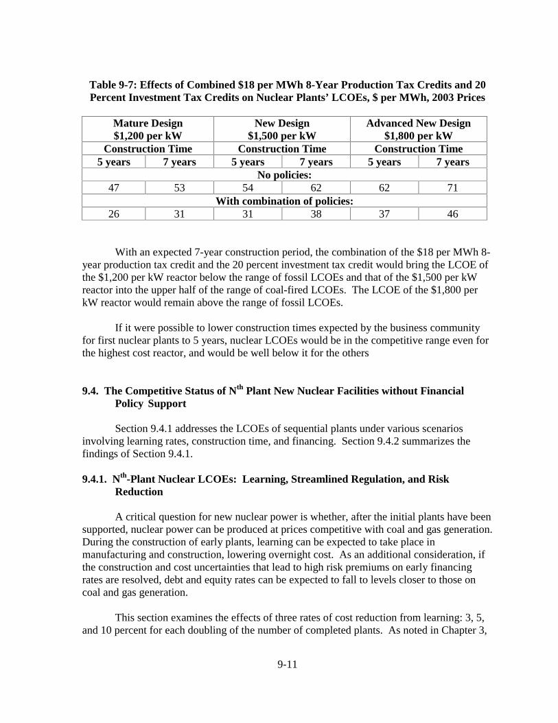
9-11

Table 9-7: Effects of Combined $18 per MWh 8-Year Production Tax Credits and 20Percent Investment Tax Credits on Nuclear Plants’ LCOEs, $ per MWh, 2003 Prices

Mature Design$1,200 per kW

New Design$1,500 per kW

Advanced New Design$1,800 per kW

Construction Time Construction Time Construction Time5 years 7 years 5 years 7 years 5 years 7 years

No policies:47 53 54 62 62 71

With combination of policies:26 31 31 38 37 46

With an expected 7-year construction period, the combination of the $18 per MWh 8-year production tax credit and the 20 percent investment tax credit would bring the LCOE ofthe $1,200 per kW reactor below the range of fossil LCOEs and that of the $1,500 per kWreactor into the upper half of the range of coal-fired LCOEs. The LCOE of the $1,800 perkW reactor would remain above the range of fossil LCOEs.

If it were possible to lower construction times expected by the business communityfor first nuclear plants to 5 years, nuclear LCOEs would be in the competitive range even forthe highest cost reactor, and would be well below it for the others

9.4. The Competitive Status of Nth Plant New Nuclear Facilities without Financial Policy Support

Section 9.4.1 addresses the LCOEs of sequential plants under various scenariosinvolving learning rates, construction time, and financing. Section 9.4.2 summarizes thefindings of Section 9.4.1.

9.4.1. Nth-Plant Nuclear LCOEs: Learning, Streamlined Regulation, and Risk Reduction

A critical question for new nuclear power is whether, after the initial plants have beensupported, nuclear power can be produced at prices competitive with coal and gas generation.During the construction of early plants, learning can be expected to take place inmanufacturing and construction, lowering overnight cost. As an additional consideration, ifthe construction and cost uncertainties that lead to high risk premiums on early financingrates are resolved, debt and equity rates can be expected to fall to levels closer to those oncoal and gas generation.

This section examines the effects of three rates of cost reduction from learning: 3, 5,and 10 percent for each doubling of the number of completed plants. As noted in Chapter 3,

9-12

3 percent is the safest rate of cost reduction to assume. Five percent would be optimistic.Ten percent would be aggressive, but may not be out of the realm of possibility. Beforeproceeding to the full array of cost-reducing effects that could be expected from thesuccessful construction of the first eight new plants, Table 9-8 provides a starting point byshowing the effects only of the payment of FOAKE costs and learning. To show the separatecontributions of FOAKE payment and learning, the LCOE of the second plant is calculatedunder two assumptions: in the first of the rows reporting LCOEs for the second plant, onlyFOAKE costs are paid after the first plant, and no learning occurs; in the second of the rowsreporting LCOEs for the second plant, the learning effect is added to the FOAKE paymenteffect. In all subsequent plants, the FOAKE cost has been paid with the construction of thefirst plant, and the benefits of cumulative learning effects are experienced.

Comparing the two lines for the second plants, the payment of FOAKE costs alonereduces the LCOEs of the $1,500 and $1,800 per kW plants by $9 per MWh. There is noeffect on the $1,200 per kW plant because its FOAKE costs were assumed to have been paidin previous construction. The addition of learning effects contributes another reduction of $2per MWh for the $1,200 and $1,500 per kW plants and an additional $ 2 to $5 per MWh forthe $1,800 per kW plant, depending on the learning rate. Continuing through the first eightplants, payment of FOAKE costs and learning effects, taken together but with no otherbenefits of building new plants, could bring the $1,200 and $1,500 per kW plants into theupper end of the competitive range with coal- and gas-fired plants with a learning rate of10 percent, but not with lesser learning rates. The LCOE of the $1,800 per kW plant remainsoutside the competitive range at the eighth plant, even under a 10 percent learning rate.

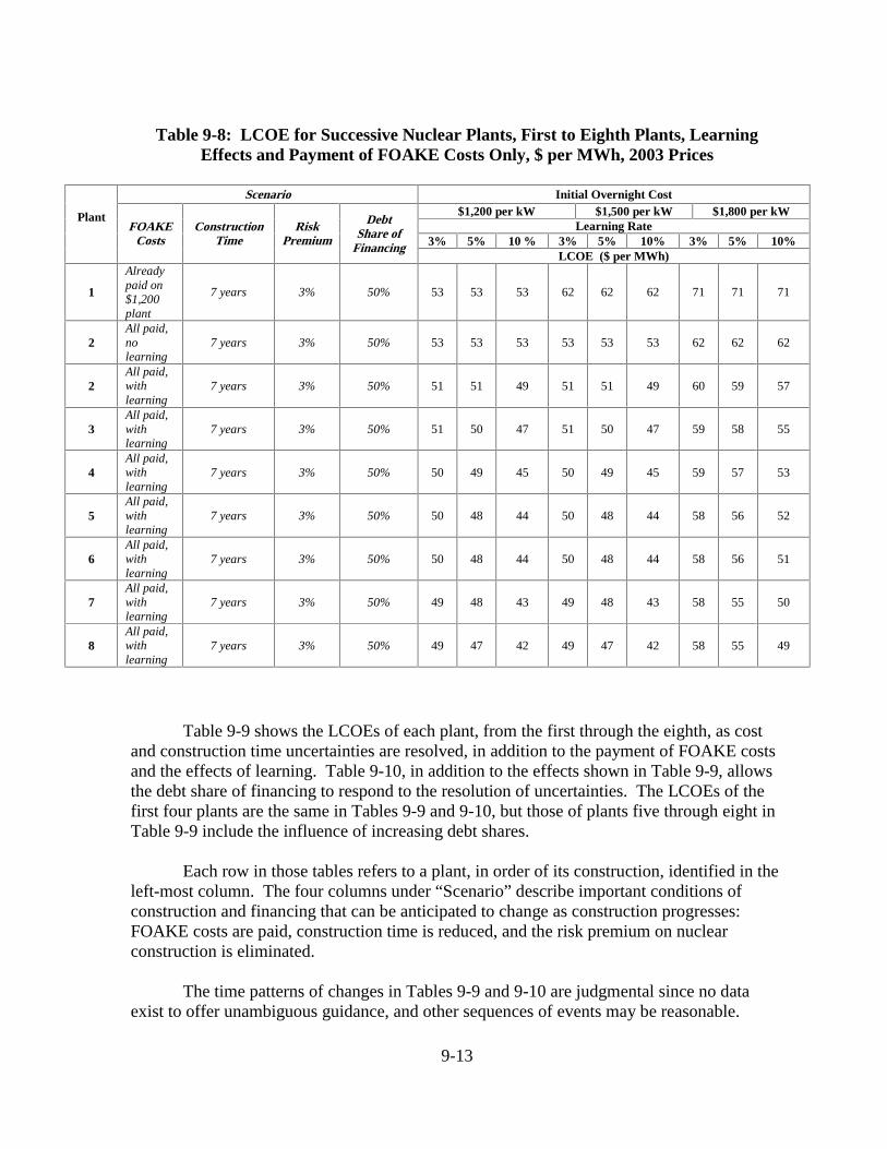
9-13

Table 9-8: LCOE for Successive Nuclear Plants, First to Eighth Plants, LearningEffects and Payment of FOAKE Costs Only, $ per MWh, 2003 Prices

Scenario Initial Overnight Cost$1,200 per kW $1,500 per kW $1,800 per kW

Learning Rate3% 5% 10 % 3% 5% 10% 3% 5% 10%

PlantFOAKE

CostsConstruction

TimeRisk

Premium

DebtShare of

FinancingLCOE ($ per MWh)

1

Alreadypaid on$1,200plant

7 years 3% 50% 53 53 53 62 62 62 71 71 71

2All paid,nolearning

7 years 3% 50% 53 53 53 53 53 53 62 62 62

2All paid,withlearning

7 years 3% 50% 51 51 49 51 51 49 60 59 57

3All paid,withlearning

7 years 3% 50% 51 50 47 51 50 47 59 58 55

4All paid,withlearning

7 years 3% 50% 50 49 45 50 49 45 59 57 53

5All paid,withlearning

7 years 3% 50% 50 48 44 50 48 44 58 56 52

6All paid,withlearning

7 years 3% 50% 50 48 44 50 48 44 58 56 51

7All paid,withlearning

7 years 3% 50% 49 48 43 49 48 43 58 55 50

8All paid,withlearning

7 years 3% 50% 49 47 42 49 47 42 58 55 49

Table 9-9 shows the LCOEs of each plant, from the first through the eighth, as costand construction time uncertainties are resolved, in addition to the payment of FOAKE costsand the effects of learning. Table 9-10, in addition to the effects shown in Table 9-9, allowsthe debt share of financing to respond to the resolution of uncertainties. The LCOEs of thefirst four plants are the same in Tables 9-9 and 9-10, but those of plants five through eight inTable 9-9 include the influence of increasing debt shares.

Each row in those tables refers to a plant, in order of its construction, identified in theleft-most column. The four columns under “Scenario” describe important conditions ofconstruction and financing that can be anticipated to change as construction progresses:FOAKE costs are paid, construction time is reduced, and the risk premium on nuclearconstruction is eliminated.

The time patterns of changes in Tables 9-9 and 9-10 are judgmental since no dataexist to offer unambiguous guidance, and other sequences of events may be reasonable.

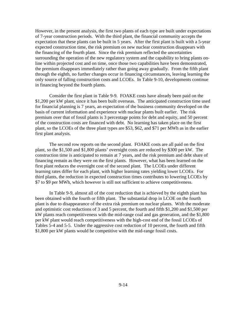
9-14

However, in the present analysis, the first two plants of each type are built under expectationsof 7-year construction periods. With the third plant, the financial community accepts theexpectation that these plants can be built in 5 years. After the first plant is built with a 5-yearexpected construction time, the risk premium on new nuclear construction disappears withthe financing of the fourth plant. Since the risk premium reflected the uncertaintiessurrounding the operation of the new regulatory system and the capability to bring plants on-line within projected cost and on time, once those two capabilities have been demonstrated,the premium disappears immediately rather than going away gradually. From the fifth plantthrough the eighth, no further changes occur in financing circumstances, leaving learning theonly source of falling construction costs and LCOEs. In Table 9-10, developments continuein financing beyond the fourth plants.

Consider the first plant in Table 9-9. FOAKE costs have already been paid on the$1,200 per kW plant, since it has been built overseas. The anticipated construction time usedfor financial planning is 7 years, an expectation of the business community developed on thebasis of current information and experience with nuclear plants built earlier. The riskpremium over that of fossil plants is 3 percentage points for debt and equity, and 50 percentof the construction costs are financed with debt. No learning has taken place on the firstplant, so the LCOEs of the three plant types are $53, $62, and $71 per MWh as in the earlierfirst plant analysis.

The second row reports on the second plant. FOAKE costs are all paid on the firstplant, so the $1,500 and $1,800 plants’ overnight costs are reduced by $300 per kW. Theconstruction time is anticipated to remain at 7 years, and the risk premium and debt share offinancing remain as they were on the first plants. However, what has been learned on thefirst plant reduces the overnight cost of the second plant. The LCOEs under differentlearning rates differ for each plant, with higher learning rates yielding lower LCOEs. Forthird plants, the reduction in expected construction times contributes to lowering LCOEs by$7 to $9 per MWh, which however is still not sufficient to achieve competitiveness.

In Table 9-9, almost all of the cost reduction that is achieved by the eighth plant hasbeen obtained with the fourth or fifth plant. The substantial drop in LCOE on the fourthplant is due to disappearance of the extra risk premium on nuclear plants. With the moderateand optimistic cost reductions of 3 and 5 percent, the fourth and fifth $1,200 and $1,500 perkW plants reach competitiveness with the mid-range coal and gas generation, and the $1,800per kW plant would reach competitiveness with the high-cost end of the fossil LCOEs ofTables 5-4 and 5-5. Under the aggressive cost reduction of 10 percent, the fourth and fifth$1,800 per kW plants would be competitive with the mid-range fossil costs.

9-15

Table 9-9: LCOE for Successive Nuclear Plants, First to Eighth Plants,$ per MWh, 2003 Prices

Scenario Initial Overnight Cost$1,200 per kW $1,500 per kW $1,800 per kW

Learning Rate3% 5% 10% 3% 5% 10% 3% 5% 10%

PlantFOAKE

CostsConstruction

TimeRisk

Premium

DebtShare of

FinancingLCOE ($ per MWh)

1

Alreadypaid on$1,200plant

7 years 3% 50% 53 53 53 62 62 62 71 71 71

2 All paid 7 years 3% 50% 51 51 49 51 51 49 60 59 573 All paid 5 years 3% 50% 45 44 42 45 44 42 52 51 484 All paid 5 years Gone 50% 36 35 33 36 35 33 41 40 375 All paid 5 years Gone 50% 35 34 32 35 34 32 40 39 366 All paid 5 years Gone 50% 35 34 32 35 34 32 40 39 367 All paid 5 years Gone 50% 35 34 31 35 34 31 40 39 358 All paid 5 years Gone 50% 35 34 31 35 34 31 40 38 35

In Table 9-10, the debt share of financing responds to the reduced uncertainties dispelled bythe successful construction of the first four plants. Financing of the fifth and sixth plants can beaccomplished with a greater proportion of debt, 60 rather than the 50 percent of the first four plants.The debt share rises to 70 percent for plants seven and eight, reducing LCOEs for those plants by afurther 5 to 10 percent.

Table 9-10: LCOE for Successive Nuclear Plants, First to Eighth Plants, with DebtShare Responding to Reduced Risk, $ per MWh, 2003 Prices a

Scenario Initial Overnight Cost$1,200 per kW $1,500 per kW $1,800 per kW

Learning Rate3% 5% 10% 3% 5% 10% 3% 5% 10%

Plant FOAKECosts,status

ConstructionTime

RiskPremium

Debt Shareof

FinancingLCOE ($ per MWh)

1

Alreadypaid on$1,200plant.

7 years 3% 50% 53 53 53 62 62 62 71 71 71

2 All paid 7 years 3% 50% 51 51 49 51 51 49 60 59 573 All paid 5 years 3% 50% 45 44 42 45 44 42 52 51 484 All paid 5 years Gone 50% 36 35 33 36 35 33 41 40 375 All paid 5 years Gone 60% �� �� �� �� �� �� �� �� ��

6 All paid 5 years Gone 60% �� �� �� �� �� �� �� �� ��

7 All paid 5 years Gone 70% �� �� �� �� �� �� �� �� ��

8 All paid 5 years Gone 70% �� �� �� �� �� �� �� �� ��

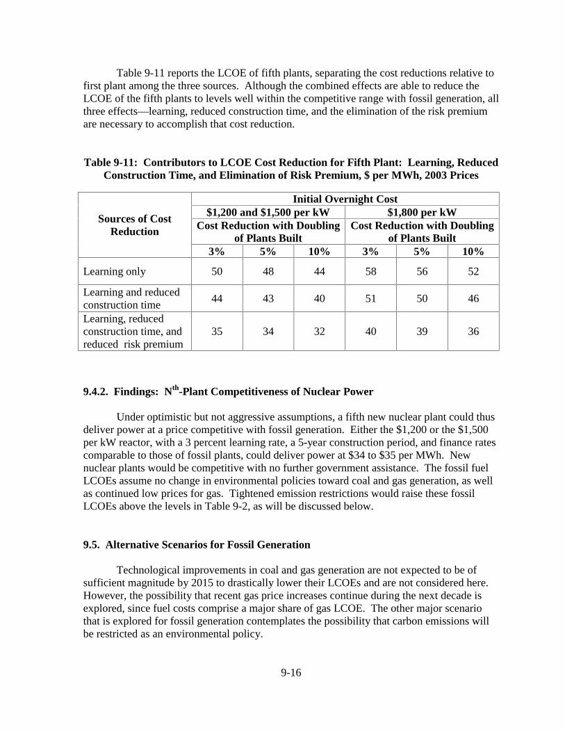
9-16

Table 9-11 reports the LCOE of fifth plants, separating the cost reductions relative tofirst plant among the three sources. Although the combined effects are able to reduce theLCOE of the fifth plants to levels well within the competitive range with fossil generation, allthree effects—learning, reduced construction time, and the elimination of the risk premiumare necessary to accomplish that cost reduction.

Table 9-11: Contributors to LCOE Cost Reduction for Fifth Plant: Learning, ReducedConstruction Time, and Elimination of Risk Premium, $ per MWh, 2003 Prices

Initial Overnight Cost$1,200 and $1,500 per kW $1,800 per kW

Cost Reduction with Doublingof Plants Built

Cost Reduction with Doublingof Plants Built

Sources of CostReduction

3% 5% 10% 3% 5% 10%

Learning only 50 48 44 58 56 52

Learning and reducedconstruction time

44 43 40 51 50 46

Learning, reducedconstruction time, andreduced risk premium

35 34 32 40 39 36

9.4.2. Findings: Nth-Plant Competitiveness of Nuclear Power

Under optimistic but not aggressive assumptions, a fifth new nuclear plant could thusdeliver power at a price competitive with fossil generation. Either the $1,200 or the $1,500per kW reactor, with a 3 percent learning rate, a 5-year construction period, and finance ratescomparable to those of fossil plants, could deliver power at $34 to $35 per MWh. Newnuclear plants would be competitive with no further government assistance. The fossil fuelLCOEs assume no change in environmental policies toward coal and gas generation, as wellas continued low prices for gas. Tightened emission restrictions would raise these fossilLCOEs above the levels in Table 9-2, as will be discussed below.

9.5. Alternative Scenarios for Fossil Generation

Technological improvements in coal and gas generation are not expected to be ofsufficient magnitude by 2015 to drastically lower their LCOEs and are not considered here.However, the possibility that recent gas price increases continue during the next decade isexplored, since fuel costs comprise a major share of gas LCOE. The other major scenariothat is explored for fossil generation contemplates the possibility that carbon emissions willbe restricted as an environmental policy.

9-17

9.5.1. Higher Natural Gas Prices

EIA’s projection for natural gas prices sees a one-third increase in real price by 2020.The gas price used in the low end of the LCOE calculations of Table 9-2 is $3.39 perMMBtu. A gas price of $4.25 to $4.30 per MMBtu would yield an LCOE of $42 to $43 perMWh. New gas plants might not be built at expected prices of this level, in view of thelower cost of coal generation under these circumstances.

9.5.2. Environmental Policies for Fossil Generation

Some tightening of NOx and SO2 emissions for coal-fired and gas-fired power plantscould occur in the future, but the cost impacts of plausible further restrictions are not great.The larger unknown in future environmental policy concerns the possibility of carbonemission restrictions. Considering the complexity of grandfathering allowances in currentenvironmental regulations, a myriad of scenarios could be constructed for a policy of carbonemission limitations.

This analysis considers a system of limitations with emission permit trading butsimplifies the institutional detail. Because of the potentially high cost of transportingcaptured CO2, it is assumed that plants located immediately adjacent to suitable sequestrationsites will be the only plants to restrict their CO2 emissions, and they will sell their emissionpermits to plants that would have to transport their captured CO2. After trades, the marginalemission reduction costs will be those of carbon capture and of injection and storage. In thisway, transportation costs could be avoided.

The costs used to represent carbon capture, injection, transportation, and storage costsare taken from Table 8-4, as averages of the individual ranges for pulverized coal-combustion and gas turbine combined cycle plants. These costs are on a per-megawatt-hourbasis, so they are added to the LCOEs calculated on the basis of other cost and performanceparameters. Table 9-12 compares the coal-fired and gas-fired LCOEs with currentenvironmental regulations with LCOEs under greenhouse policy of the character describedhere. The coal-fired plant LCOE would be increased two and one-half times, while the gas-fired plant LCOE would rise by one-half.

Table 9-12: Fossil Fuel Generation LCOEs with and without Greenhouse Policies,$ per MWh, 2003 Prices

Under Current EnvironmentalPolicies

Under GreenhousePolicy

Coal-fired 33 to 41 83 to 91Gas-fired 35 to 45 58 to 68

9-18

Even if clean coal research were to reduce the carbon sequestration costs associatedwith coal plants by 50 percent, an LCOE of $65 per MWh could still emerge. Improvedcapture and sequestration technology for gas plants could leave the gas LCOE in the range ofthe mid-$50s per MWh. Reasonable scenarios for new nuclear power would yield LCOEscompetitive with such coal and gas costs.

While stringent greenhouse policies would very likely make nuclear powercompetitive on its own, the policy analysis in this chapter concerned with 2015 does not relyon them. Implications of greenhouse policies for the 2025 and beyond are considered in thenext chapter.

9.6. Conclusions

Among the financial instruments considered in this study, production tax credits aremost effective in reducing LCOEs, followed by investment tax credits. Loan guarantees andaccelerated depreciation are less effective. Starting from the no-policy benchmarks LCOEsof $53, $62, and $71 per MWh for $1,200, $1,500 and $1,800 per kW reactors, only oneindividual financial policy in isolation (the $18 per MWh production tax credit over 8 years,applied to a $1,200 per kW reactor) would bring these reactor designs’ costs for a firstnuclear plant within the competitive range with fossil fuel power generation of $35 to $45per MWh. However, the production tax credit is a back-end policy that achievescompetitiveness through increasing net revenues from sales after the plant is constructed. Itdoes not provide front-end dollars in the here and now of the construction period to whichgreater weight would be given.

Still considering first new nuclear plants, applying two policies together as a package,yields a policy combination that could bring two of the reactor designs well into acompetitive LCOE range with fossil-fired generation. A combination of an investment taxcredit of 20 percent and an $18 per MWh production tax credit applied for 8 years issufficient to bring the $1,200 and $1,500 per kW reactors within the competitive cost range.That policy package would let the more costly $1,800 per kW reactor reach competitive costlevels if investors were convinced that a first plant could be built in 5 years.

This analysis for first nuclear plants has concentrated on results to be expectedassuming an expectation of a 7-year construction period and added debt and equity riskpremiums of 3 percent, reflecting business attitudes found in the Scully Capital report as wellas anecdotal evidence. Financial policies have been analyzed under these assumptions. Wehave emphasized that actual experience may turn out to be more favorable. If it werepossible to find investors willing to accept the likelihood of a more favorable outcome, theneed for financial assistance would be reduced, even conceivably eliminated. One-timeguarantees of construction costs, or DOE construction and sale of plants, are examples ofpolicies going beyond the type of traditional financial measures considered here that could beconsidered to overcome business concerns about nuclear plant risk. It is beyond the scope ofthe present study to consider the pros, cons, and realism of these types of measures for firstnew nuclear plants.

9-19

Consider finally the competitiveness of later nuclear plants. Learning effects can beexpected to reduce overnight capital costs. Successful construction and operationexperience, aided by streamlined regulation, should reduce expected construction time andalso permit a reduction of risk premiums. With learning rates of 3 to 5 percent, constructionperiods of 5 years, and financing rates comparable to those of fossil plants, the $1,200 and$1,500 per kW reactors would be competitive with fossil power by the fifth plant. Ifsuccessful contractor and operator experience with early plants permitted the reduction ofrisk premiums on debt and equity finance for fifth plants, both of these reactors wouldoperate well within the competitive range, and the $1,800 per kW reactor would reach theupper end of the competitive range. The results suggest that nuclear power could becomecompetitive on its own after a fairly brief period of policy assistance.

9-20

References

Abraham, Spencer. (2004). Luncheon Address to the Keidanren, Tokyo, Japan. January 9.

Bush, George W. (2004) Statement to students at Niles High School. Niles, Mich., May 24.Retrieved from Worldwide Web May 2004: http://www.nei.org/doc.asp?docid=1196.

Davis, G., and B. Owens. (2003) “Optimizing the Level of Renewable Electric R&DExpenditures Using Real Options Analysis.” NREL/TP-620-31221. Golden, Colorado:National Renewable Energy Laboratory, February.

Dixit, Avinash K., and Robert S. Pindyck. (1994) Investment Under Uncertainty.Princeton: Princeton University Press.

Energy Information Administration (EIA). (2002) Annual Energy Review. Retrieved fromthe World Wide Web January 2004: http://www.eia.doe.gov/emeu/aer/txt/ptb0602.html,http://www.eia.doe.gov/emeu/aer/txt/ptb0603.html.

Energy Information Administration (EIA). (2003a) Annual Energy Outlook 2003.Washington, D.C.: U.S. Department of Energy.

Energy Information Administration (EIA). (2003b) Retrieved September 10, 2003 from theWorld Wide Web: www.eia.doe.gov/emeu/international/ngasprie.html.

Energy Information Administration (EIA). (2003c) Retrieved September 10, 2003 from theWorld Wide Web: www.eia.doe.gov/emeu/international/ngasprii.html.

Energy Information Administration (EIA). (2003d) Retrieved September 10, 2003 from theWorld Wide Web: www.eia.doe.gov/emeu/international/ngasprih.html.

Energy Information Administration (EIA). (2004a) Annual Energy Outlook 2004 withProjection to 2025. Washington D.C.: Energy Information Administration, January.Supplemental tables retrieved from the World Wide Web January 2004:http://www.eia.doe.gov/oiaf/aoe/excel/aeo_base.xls

Energy Information Administration (EIA). (2004b) Retrieved June 2004 from the WorldWide Web: http://tonto.eia.doe.gov/dnav/ng/hist/n9070us2a.htm.

Energy Information Administration (EIA). (2004c) Retrieved June 2004 from the WorldWide Web: http://tonto.eia.doe.gov/dnav/ng/hist/n9100us2A.htm.

Energy Research Board (ERB). (2001) “Canadian Natural Gas: Market Review andOutlook.” Canada. Retrieved January 7, 2004 from the World Wide Web:http://www2.nrcan.gc.ca/es/erb/prb/english/View.asp?x=447&oid=651.

9-21

Fisher, William L. (1994) “How Technology Has Confounded U.S. Gas ResourceEstimators,” Oil & Gas Journal 92, October 24: 100-107.

Greenspan, Alan. (2003) “Natural Gas Supply.” Testimony before Senate Committee onEnergy and Natural Resources, Federal Reserve Board.

Guillerminet, Maire-Laure. (2001) “La décision d’investissement en électricité et sonfinancement dans un environmennement institutionnel en mutation.” Mimeo. Paperpresented at Colloque international “La nécessité de nouvelles régulations internationalesface aux mutations énergétiques et environmennementales,” Paris, June 10-13. Downloadedfrom Worldwide Web December 2003: http://www.sceco.univ-montp1.fr/creden/Reseau/DOCS%20COLLOQUE/M_L_Guillerminet. pdf.

Hamilton, James D. (1983) “Oil and the Macroeconomy since World War II,” Journal ofPolitical Economy 91: 228-248.

Jensen, James T. (2003) “The LNG Revolution,” The Energy Journal 24, No. 2: 1-45.

Jones, Donald W., Inja K. Paik, and Paul N. Leiby. (2004) “Oil Price Shocks and theMacroeconomy: What Has Been Learned Since 1996,” forthcoming in The Energy Journal25, No. 2: 1-32.

National Energy Policy Development Group (NEPDG). (2001) National Energy Policy:Reliable, Affordable, and Environmentally Sound Energy for America’s Future. Report ofthe National Energy Policy Development Group. Washington, D.C.: U.S. GovernmentPrinting Office, May.

National Petroleum Council (NPC). (1999) “Meeting the Challenges of the Nation’sGrowing Natural Gas Demands.” Washington, D.C., December 1999.

National Petroleum Council (NPC). (2003) “Balancing Natural Gas Policy – Fueling theDemands of a Growing Economy.” Washington, D.C., September 2003.

Pindyck, Robert S. (1991) “Irreversibility, Uncertainty, and Investment,” Journal ofEconomic Literature 29: 1110-1148.

Schimmelpfennig, D. (1995) “The Option Value of Renewable Energy: The Case ofClimate Change,” Energy Economics 17: 311-317.

Schmoker, James W., and Thaddeus S. Dyman. (2001) Changing Perceptions of UnitedStates Natural Gas Resources as Shown by Successive U.S. Department of the InteriorAssessments. U.S.Geological Survey Bulletin 2172-B. Washington, D.C.: U.S. GeologicalSurvey.

9-22

Simmons, M.R. (2003) “Future Energy Resources: Are We Asking the Right Questions.”National Defense University Workshop, Simmons International.

Smith, R., and A. Hove. (2003) “Utilities: The Old Reliables.” Deutsche Bank AG.

Stokey, Nancy L., and Robert E. Lucas, Jr., with Edward C. Prescott. (1989) RecursiveMethods in Economic Dynamics. Cambridge, Mass.: Harvard University Press.

U.S. Department of Energy (DOE) and Nuclear Power Industry. (2004). Strategic Plan forLight Water Reactor Research and Development. First Edition. Washington, D.C.: Officeof Nuclear Energy, Science and Technology; Nuclear Energy Institute, and Electric PowerResearch Institute, February.

Webber, Jude. (2003) “Bolivia May Miss the Boat on Natural Gas Exports,” Reuters,October 20. Retrieved December 2003 from the World Wide Web:http://www.latinpetroleum.com/article_2295.shtml.

10-1

Chapter 10. NUCLEAR ENERGY SCENARIOS: BEYOND 2015

Summary

The long gestation periods involved in nuclear research, the long lags entailed ingearing up the nuclear industry for production, to say nothing of the long-term nature ofsecurity and environmental problems bearing on nuclear energy, make it prudent to attemptto look several decades ahead in making decisions about nuclear energy policy.

Uncertainties of virtually every kind increase as a longer time horizon is considered.While achieving precision becomes increasingly difficult as one attempts to look out fartherto the future, the direction of some events has been persistent over the past few decades andshows every sign of continuing. These include perhaps most clearly the continued growth indemand for electricity and continued growth in severity of environmental problems. Beyondthese, all the policy concerns addressed in Part Two above seem likely to continue. Thelikelihood that they will become more serious seems great.

Exhaustive consideration is not feasible here. The present study closes byconsidering three matters of particular importance for 2025 and beyond, having implicationsfor nuclear energy strategies now.

First is nuclear energy technology. Much is already known about the momentum ofnuclear cost reductions using existing technology. Much is also known about nuclear energyR&D on new technologies that will come to fruition after 2025. The R&D is ongoing andmust be planned years ahead.

The importance of cost reductions from first-of-a-kind-engineering (FOAKE) costsand learning by doing beyond FOAKE has been verified above in Part Three. There is everyreason to believe that this type of experience will continue. If presently available GenerationIII technologies are deployed for several years beginning in 2015, as contemplated in thisstudy, cost reductions from their replication could extend to 2025 and beyond.

New designs from R&D work on Generations III+ and IV reactors, with manyspecifics now already in motion, may be commercialized soon after 2025. R&D in generalhas the potential to reduce costs. Cost reduction will be a prerequisite to commercialization.

The Pebble Bed Modular Reactor (PBMR), a relatively near-term technology, couldmake a particular contribution to reducing costs in view of its modularity. With independentunits of 110 MW, an 1,100 MW power plant could be constructed in a sequence permittingunits begun earlier to be brought on line earlier. Interest during construction, which hasnormally accounted for one quarter of nuclear LCOE, could be greatly reduced, perhaps evento minor proportions. Furthermore, once proof-of-principle was established, the smalleramounts of capital at risk in a single project__viewing the individual units as separateprojects__would reduce the risk premium that larger projects now have to pay. The

10-2

advantages of modular construction might be enough by themselves to make nuclear powerself-sufficient in the marketplace.

A more general lesson is that attention to potentials for cost reductions as a majorconsideration in planning nuclear R&D directions will increase the likelihood of commercialviability. The findings emphasized in this study, that reducing construction time and riskpremiums greatly reduce nuclear energy costs, underscore this lesson.

A second major consideration is global warming. The longer the time horizon in thefuture that is considered, the more likely it is that the priority given to global warming willincrease, leading to urgent need to replace coal- and gas-fired electricity generation. In viewof the time it takes to gear up the nuclear industry, this eventuality is one of the reasons fornational concern with maintaining a nuclear energy capability.

As one considers years increasingly farther beyond 2025, the probability grows evergreater that global warming will be perceived, not just as a potential threat, but rather as areality calling for stringent action. If this view is accepted, the prospect of environmentalpolicies greatly restricting carbon emissions in the period after 2025 must be admitted as anincreasingly real possibility. Even if carbon capture and sequestration technologies areimproved, and their costs reduced, a requirement that fossil power plants capture carboncould increase their LCOEs by 50 to 100 percent over current levels. Nuclear power wouldthen acquire an unquestioned advantage over its gas and coal competitors.

A third major consideration is hydrogen. As brought out in Appendix A8, thewidespread introduction of hydrogen-powered vehicles to replace gasoline-powered vehicleswould greatly increase the demand for energy to produce hydrogen. Some impacts couldoccur by 2015, but these were conservatively not considered in projecting demand fornuclear energy by 2015 in the present study. Assuming success in meeting the expressednational commitment to developing a commercially viable hydrogen vehicle, use of hydrogenvehicles will be widespread by 2025 and beyond.

The possibility exists that heat from nuclear reactors will be the energy source ofchoice for producing hydrogen. Alternative possibilities include continued use of steammethane reforming and electrolysis using electricity from fossil generation. However, thecarbon emissions from these sources would be acting simply to replace the reduction incarbon emissions from displacement of gasoline-powered vehicles. If there were seriousrestrictions on the use of coal and gas because of their carbon emissions, nuclear energywould have a clear competitive edge. A full analysis of the implications of increased demandfor hydrogen is beyond the scope of this study. Still, the point again is that a contingencythat could become real by 2025 could favor the demand for nuclear power.

While many uncertainties cloud the future beyond 2025 in addition to thoseconsidered, the uncertainties bearing on nuclear energy that emerge from the present studysuggest the likelihood of an increased demand for nuclear energy beyond 2025.

10-3

Outline

10.1 Introduction

10.2. Reactor Costs

10.2.1. Nth -of-a-Kind Costs10.2.2. New Reactor Designs

10.3. Environmental Policies

10.4. New Demands for Electricity: The Hydrogen Economy

10.5. Conclusion

10-4

10.1. Introduction

While the future beyond 2025 clearly holds many uncertainties, this chapter identifiesthree particular areas which could affect nuclear power. Continued experience inconstruction and operation of the Generation III reactors built by 2015 can be expected tocontinue lowering their costs. Generation IV reactor designs are expected to still be indemonstration stages in 2015, and some may still be in research stages. Some GenerationIII+ or early Generation IV designs may reach commercialization by 2025 or soon after.Section 10.2 addresses developments in these areas.

As a non-polluting electricity source, nuclear power can be expected to benefit fromtightening of environmental policies on fossil generation. Section 10.3 considers the futureof environmental policies.

A third major area of uncertainty affecting nuclear power in the more distant future isthe possible emergence of a hydrogen economy. Large-scale substitution of hydrogen for oilin the transportation sector could increase the demand either for heat or for electricitysubstantially. Producing hydrogen by steam methane reforming would release carbonemissions that would have been emitted otherwise from the direct burning of oil, makingnuclear power a more attractive source of hydrogen production. Section 10.4 addresseshydrogen issues.

10.2. Reactor Costs

The cost of nuclear reactors almost certainly will continue to be a major concern inthe commercial nuclear power industry. Two major sources of cost reductions in the post-2025 period will be continued learning on the reactor designs built between 2015 and 2025,and the introduction of some cost-effective designs not yet commercialized.

10.2.1. Nth-of-a-Kind Costs

Cost reductions from learning, in both component manufacturing and construction,can be expected to continue, although the exponential learning rate—the rule of thumb of aconstant percentage cost reduction with every doubling of new plants—will attenuate thelearning effect of each new plant. A constant 3 percent learning rate with plant doublingwould bring the overnight cost of a $1,200 per kW first-cost reactor down to $1,000 per kWby the sixty-fourth plant, and a 5 percent learning rate would reduce the same overnight costto $880 per kW. Over the next quarter century 64 new plants could easily be built.

10.2.2. New Reactor Designs

Generation IV reactors include a variety of advanced designs, but the cost at whichthey can deliver electricity will continue to be an overriding concern in theircommercialization. The Pebble Bed Modular Reactor (PBMR) is one of the nearer-term

10-5

designs, and its modularity could confer cost advantages. With independent units of 110MW, an 1,100 MW power plant could be constructed in a sequence that permitted unitsbegun earlier to be brought on line earlier, reducing construction interest. Beyond thatadvantage, once its proof-of-principle was established, the smaller amounts of capital at riskin a single project—viewing the individual units as separate projects—could reduce the riskpremium that larger projects might have to pay.

10.3. Environmental Policies

The longer the time horizon in the future that is considered, the more likely it is thatglobal warming will become a pre-eminent concern, leading to urgent need to replace coal-and gas-fired electricity generation. In view of the time it takes to gear up the nuclearindustry, this eventuality is one of the reasons for national concern with maintaining anuclear energy capability.

The LCOEs calculated in Chapter 9 for coal and gas generation under potentialgreenhouse policies may be high compared to the technology that actually emerges in thenext several decades, but indicate that even with major cost reductions in meetingenvironmental goals from fossil electricity generation, nuclear power would be the morecompetitive electricity source.

10.4. New Demands for Electricity: The Hydrogen Economy

If hydrogen were to make a major inroad on oil in transportation fuels, how toproduce the hydrogen could prove to be a major issue. As reported in Appendix A8,production of hydrogen using steam methane reforming is capable of reducing carbonemissions on balance, although production by electrolysis at coal plants would increase thoseemissions. Producing hydrogen with nuclear power by thermo-chemical processes wouldemit no carbon, offering a 100 percent reduction in carbon emissions with no take-backeffect through the hydrogen production.

Of the currently available methods of producing hydrogen, electrolysis, which wouldrequire considerable electricity, has not been tried at large scales of production. Steammethane reforming, the current production method of choice, needs process heat that couldbe supplied by either gas or nuclear reactors, but its economic viability is subject to the priceof its feedstock, and its production emits carbon unless steps are taken to capture it. Thermalwater-splitting is an alternative, non-carbon-emitting chemical process, and it can bepowered by nuclear energy.

Nuclear reactors produce large amounts of heat that can be used for a variety ofapplications. The addition of a gas or steam turbine would allow production of electricity.Adding a thermo-chemical water splitting unit would permit hydrogen production. Lookingto the post-2025 future, variations on modular helium reactors such as the GT-MHR

10-6

described in Appendix A4, may be candidates for supplying the process heat for hydrogenproduction. The Very High Temperature Reactor (VHTR), the next generation modularhelium reactor (MHR), consists of 600 MW (thermal) modules specially designed to supplythe required heat for thermo-chemical water splitting processes while avoiding tritiumcontamination of hydrogen (Schultz 2003, p.4; Southworth 2002). The Advanced HighTemperature Reactor (AHTR) is an alternative to the MHR concept, as it is very large(2,400 MW) and uses a molten salt coolant as opposed to helium (Forsberg 2003, p. 1077).Both, however, require additional research in high temperature materials and integration withhydrogen production techniques before commercialization is possible.

10.5. Conclusion

While many uncertainties cloud the future beyond 2025 in addition to thoseconsidered, the uncertainties bearing on nuclear power that emerge from the present studysuggest the likelihood of an increased demand for nuclear power beyond 2025.

10-7

References

Forsberg, Charles W. (2003) “Hydrogen, Nuclear Energy, and the Advanced High-Temperature Reactor,” International Journal of Hydrogen Energy 28: 1073-1081.

Schultz, K.R. (2003) “Use of the Modular Helium Reactor for Hydrogen Production.” SanDiego: General Atomics. Retrieved December 2003 from the World Wide Web:http://www.world-nuclear.org/sym/2003/pdf/schultz.pdf.

Southworth, Finis. (2002) “Very High Temperature Gas Cooled Reactor Systems.”Presentation to American Nuclear Society (ANS) Winter Meeting, Washington, D.C. IdahoNational Engineering & Environmental Laboratory, November.

10-8

Appendix: Major Issues Affecting the Nuclear Power Industry inthe U.S. Economy

A1-2

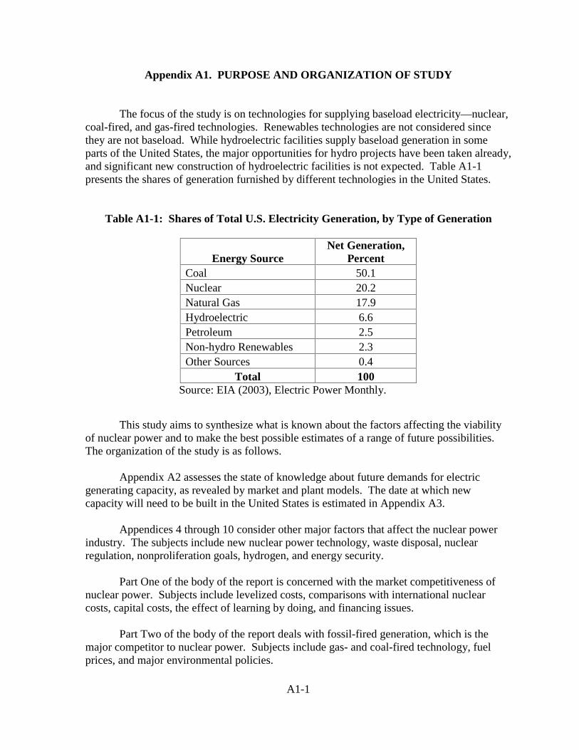
A1-1

Appendix A1. PURPOSE AND ORGANIZATION OF STUDY

The focus of the study is on technologies for supplying baseload electricity—nuclear,coal-fired, and gas-fired technologies. Renewables technologies are not considered sincethey are not baseload. While hydroelectric facilities supply baseload generation in someparts of the United States, the major opportunities for hydro projects have been taken already,and significant new construction of hydroelectric facilities is not expected. Table A1-1presents the shares of generation furnished by different technologies in the United States.

Table A1-1: Shares of Total U.S. Electricity Generation, by Type of Generation

Energy SourceNet Generation,

PercentCoal 50.1Nuclear 20.2Natural Gas 17.9Hydroelectric 6.6Petroleum 2.5Non-hydro Renewables 2.3Other Sources 0.4

Total 100Source: EIA (2003), Electric Power Monthly.

This study aims to synthesize what is known about the factors affecting the viabilityof nuclear power and to make the best possible estimates of a range of future possibilities.The organization of the study is as follows.

Appendix A2 assesses the state of knowledge about future demands for electricgenerating capacity, as revealed by market and plant models. The date at which newcapacity will need to be built in the United States is estimated in Appendix A3.

Appendices 4 through 10 consider other major factors that affect the nuclear powerindustry. The subjects include new nuclear power technology, waste disposal, nuclearregulation, nonproliferation goals, hydrogen, and energy security.

Part One of the body of the report is concerned with the market competitiveness ofnuclear power. Subjects include levelized costs, comparisons with international nuclearcosts, capital costs, the effect of learning by doing, and financing issues.

Part Two of the body of the report deals with fossil-fired generation, which is themajor competitor to nuclear power. Subjects include gas- and coal-fired technology, fuelprices, and major environmental policies.

A1-2

Part Three of the body of the report develops policy scenarios for the future. The firstset of scenarios is for nuclear plants built starting in 2015, which is the projected nextrealistic time to complete a new plant. The second set of scenarios is for plants built beyond2025.

A2-1

Appendix A2. ELECTRICITY FUTURES: A REVIEW OF PREVIOUS STUDIES

Summary

Two principal types of models have been used to investigate electricity futures: plantmodels and market models. Plant models calculate the cost of electricity generation from aspecific type of power plant. Costs are calculated on a levelized basis (LCOE), combiningoperating and capital costs to arrive at a cost per kWh, which if charged will recoup the costof supplying electricity. Costs are calculated at the busbar level in order to focus onelectricity generation costs abstracting from locally varying distribution costs.

Market models forecast the demand for electricity and the mix of electricitygenerating capacity that will come online to meet future levels of expected demand.Aggregate demand and supply functions are estimated and brought together simulatingmarket behavior, often at the regional level.

By presenting cost per kWh figures, plant studies provide a useable commondenominator. If nuclear energy can enter the marketplace at a cost per kWh equal to or lessthan other baseload electric power sources, it can hope to find a niche as a major powersource. Cost per kWh is not a perfect measure inasmuch as it will be an average of actualmagnitudes that depend on local conditions.

Focusing on cost per kWh simplifies analysis by eliminating the need for elaborateprojections of the precise share of nuclear in the nation’s energy mix. The essential questionbecomes: Will nuclear power enter the marketplace as a viable baseload option? It may doso with greater or less robustness, which may vary from place to place, and if the niche is tobe expanded, will enter at a rate influenced by how fast other baseload sources are retired. Itis not necessary to consider these details, at least in the first instance. There is little point inproceeding to these details unless the prerequisite cost per kWh is achieved that is necessaryfor a viable niche.

Within each category of model, different underlying numerical assumptionscontribute to the principal differences in projections. The most significant of these aredifferences in overnight costs and interest rates for nuclear capacity, overnight costs for coalgeneration, and fuel costs for gas generation. Among the plant models, the most importantstructural difference is the inclusion or exclusion of taxes. The market models aresufficiently complex that reasons for differences in their projections frequently are difficult topinpoint. The results depend on black box calculations that the reader cannot replicate, witha resulting lack of intuition as to what is driving the results.

Plant models appear better suited to the present investigation concerned with theviability of nuclear power. Their structures are straight forward enough to permitcalculations to be transparent. Plant models however are far from being totally transparent.Frequently, plant calculations are made whose documentation is insufficient to permit

A2-2

evaluation. Later in this study, attempts are made to narrow the range of uncertaintysuggested by the sometimes wide differences in LCOE estimates from the previous studies.

A2-3

Outline

A2.1. Introduction

A2.2. Plant Models

A2.2.1. LCOE Estimation Using Plant ModelsA2.2.2. “Business Case for New Nuclear Power Plants” by Scully CapitalA2.2.3. GenSimA2.2.4. The MIT Nuclear Power Study

A2.3. Market Models

A2.3.1. Basics of Market ModelsA2.3.2. The National Energy Modeling System (NEMS)A2.3.3. The All Modular Industry Growth Assessment (AMIGA) Modeling

SystemA2.3.4. Integrated Planning Model, U.S. Environmental Protection Agency

A2.4. A Hybrid Model: SAIC’s Power Choice Model

A2.5. Conclusion

References

A2-4

A2.1. Introduction

The purpose of this appendix is to assess the models that have been used to projectnuclear generated electricity costs, nuclear shares of electric generation capacity, andaggregate electricity demand and supply. This review concentrates on recent and significantmodels. The models can be divided into two types, plant models and market models. Theplant models calculate the busbar or levelized cost of electricity (LCOE) from a single plantof a particular type. The market models project the price of electricity supplied, the types ofgenerating plants used, and the quantity of electricity supplied. In addition, the marketmodels contain, implicitly or explicitly, supply-demand interactions and decisions ofbusinesses.

Section A2.2 reviews plant electricity models. Section A2.3 reviews market models.Section A2.4 reports on a hybrid model. Section A2.5 draws conclusions for the analysis tobe undertaken in this study.

A2.2. Plant Models

Plant models focus on the economics of electricity generation from a single type ofpower plant. Called levelized-cost-of-electricity, or LCOE models, they are used to explorevarious influences on generation cost. Beyond that, they are sometimes used to provide costinformation for market models. Section A2.2.1 describes a generic plant, or LCOE, model.Section A2.2.2 reviews several specific plant models.

A2.2.1. LCOE Estimation Using Plant Models

Plant economic models of electricity generating plants are primarily concerned withpredicting the cost of electricity generation. The cost of power generation is dependent onthe cost of building, operating, and maintaining the power plant, and is commonly referred toas the levelized cost of electricity, or LCOE. The LCOE is a measure of the generation costof electricity, in constant dollars, for a plant using a particular generating technology overlifespan.

The major components of the LCOE equation are:

LCOE = Capital Cost + Operating and Maintenance Cost + Fuel Cost.

This equation includes both up-front capital costs and yearly costs that recur annuallyover the life of the plant. The LCOE calculation amortizes the capital cost components toplace them on a yearly basis comparable to the annual costs. Given the rate of returnrequired by investors, the LCOE is the price that must be received for power if costs are to becovered.

A2-5

A2.2.1.1. Capital Cost

Capital costs are treated in detail in Chapter 3, so only a brief guide to the contents ofthe capital cost component of the LCOE equation is offered here. The base for the capitalcost portion is the overnight cost for a generating plant. Overnight cost is construction costswithout interest charges. It is generally quoted in terms of dollars per kilowatt of capacity.As plants are not in fact built overnight, the total capital cost per kilowatt can vary dependingon the construction time and financing terms.

Overnight costs are not firm quotations from generating plant suppliers, but rather areestimates of the cost to build a new plant of a given type. In the case of fossil fuel plants,where plant construction occurs at a relatively steady pace, the overnight cost estimates arebased on historical costs, and variation in cost is expected to be minimal. However, becauseno new nuclear plants have been built in the United States recently, the margin of error inestimating overnight construction costs for nuclear plants is larger.

Estimates of overnight costs sometimes assume an nth-of-a-kind plant, a plant whosedesign has been built frequently enough in the past that there is little potential for furtherreductions in cost due to improvements in construction experience. Most fossil plants fallinto this category. By contrast, when a completely new type of power plant is built, it incursfirst-of-a-kind-engineering or FOAKE costs, which represent the pre-constructionengineering work required for implementing a prototype technology. Inclusion or exclusionof FOAKE costs for newer, advanced nuclear reactor designs and the lack of recent historicalexperience has contributed to considerable variability in overnight construction costestimates for new nuclear power plants. There may, in addition, be learning effects for thefirst few plants beyond the first one.

A power plant’s capacity factor, the percentage of total rated power that is used,reflects the effect of scheduled and unscheduled downtime on the total amount of power thatthe plant is able to generate in a given year. Variations in the expected capacity factor canmake a significant difference to the busbar cost of electricity, as an increase in the expectedcapacity factor has the same effect as lowering capital costs per kilowatt. Historically, U.S.nuclear power plants suffered from initially low capacity factors, but these have improved inrecent years to levels approaching 90 percent.

The expected lifespan of the plant also affects the cost of electricity, as capital costsare typically recovered over the lifespan of the plant. While power plants are designed forspecific operating lifetimes, many fossil plants are operating beyond their original designlives, and a number of nuclear plants are currently requesting license extensions andundergoing refurbishing to extend their lifespan. A longer plant life lets the capital in a plantgenerate more electricity and consequently lowers capital cost per kilowatt, but because ofdiscounting, beyond a certain point (40 years or so), increasing the expected lifespan of theplant has only a small effect on the present-value cost represented by the LCOE. Most of thecapital costs are recovered in the first 20 years of operation.

A2-6

A2.2.1.2. Yearly Operating Costs

Yearly operating expenses have to be paid as long as the plant is still operational.Many of these do not vary with the amount of power being generated. For example,employee wages, general maintenance, and overheads are in this category. They are usuallyhistorically well established and exhibit low variance. They tend to make up the smallestportion of busbar electricity costs across generation plant types. For these reasons, they arenot typically disaggregated in great detail.

Fuel costs are the major component of variable costs, since for most power planttypes the only element of cost that varies directly with the amount of power generated is fuel.Some power generation technologies such as renewables like solar and wind have zerovariable cost, but the baseload plant types—fossil and nuclear—have significant variablecosts. Fuel price is an input into a plant model, along with the plant’s heat rate, a measure ofBTUs needed to generate a kilowatt-hour of electricity. Lower heat rates correspond to moreefficient plant designs and hence lower variable costs of operation.

Many plant models use the heat rate in their calculations to allow for improvements totechnology that reduce the heat rate. In addition, different fuel types have different BTUs,which is significant for plants that can accept more than one type of fuel. For example,differing grades of coal are in use by coal-fired power plants, and each grade has a differentaverage BTU content, so the LCOE of a plant may differ according to its location because offuel costs, among other local factors.

A common assumption in LCOE models for nuclear plants is that total cost fornuclear fuel per kilowatt-hour or per year is given. This approach works satisfactorily fornuclear power, as the heat rates across previously built nuclear plants are fairly similar, andfuel costs are only a small fraction of the cost of nuclear power generation. Since nuclearplants are run as baseload at a relatively constant capacity, and the price of nuclear fuel hasbeen quite stable, the cost of nuclear fuel from year to year is predicted to be quite stable.

A2.2.1.3. Externalities

Power plants often produce unwanted byproducts, such as waste heat, greenhousegases, and toxic elements. Other less visible externalities also exist, such as spent fuel andpossible weapons proliferation effects in the case of nuclear power plants. In recent years,tightening environmental regulations have meant that power producers have to include thecost of controls to reduce these externalities – particularly SO2 and NOX – into their costcalculations. In the future, CO2 emissions may be regulated, and some models allow for thecosts of limiting those emissions.

A2.2.2. “Business Case for New Nuclear Power Plants” by Scully Capital

Scully Capital was contracted by the U.S. Department of Energy (DOE) to examinethe feasibility of new nuclear power plants from an industry and financial perspective. The

A2-7

Scully Capital report first qualitatively examines the risk factors that are critical to thenuclear plant decision, such as nuclear waste disposal, the public perception of nuclear risk,and government support. Scully Capital includes a model for calculating the economics ofnuclear power from a project financing perspective. The model is used to analyze theeconomics of investing in nuclear power, under alternative assumptions about capital costsand financing structure.

The Scully Capital model’s focus is on investors’ perceptions of profitability. Themodel solves for the internal rate of return (IRR) on equity in the investment, assuming awholesale price of baseload electricity, which is the implied LCOE received (Scully Capital2002, p.101). The results can be re-arranged to express LCOE as a function of investorrequired rate of return, which is done in Chapter 1.

The Scully Model uses EPC or Engineer-Procure-Construct costs as the base for thecapital cost of nuclear power. These costs are based on the AP1000 reactor by Westinghouseand appear to come directly from Westinghouse estimates (Scully Capital 2002, p.90). As acomponent of overnight costs, EPC costs do not contain any financing charges, but owner’scosts, contingency costs and other development costs are added to the EPC cost, addingabout 10 percent to arrive at full overnight costs before financing. A range of EPC costsfrom $1.6 billion to $1.0 billion for a 1,100 MW reactor is used, the range reflectingimprovements in technology and construction experience that could eventually reduce thecost of construction. Translated into per kW terms, the resulting cost range is $909 to $1,454per kW.

A2.2.3. GenSim

The GenSim model from Sandia National Laboratories (Drennan et al. 2002) is ageneric LCOE model. The LCOE calculation is (Drennan et al. 2002, p. 10)

,&)(

Q

E

Q

MO

Q

CRFILCOE ++=

where I is capital investment, including finance costs; CRF is the capital recovery factor,

specified as 1)1(

)1(

−++=

n

n

r

rrCRF , in which r is the real discount rate and n is the plant life; Q

is annual plant output in kilowatt hours; O&M is fixed and variable operation andmaintenance costs; and E is externality costs. The report identifies F as fuel costs, but theterm does not appear in the published version of the report on the model. Presumably a term+F/Q is omitted from the reported equation rather than from the actual model. The model iswritten in the software package Powersim Constructor (Drennan et al. 2002, p. 7).

The technologies for which the model has calculated LCOEs include nuclear, coal,gas combined cycle, solar photovoltaic, solar thermal, and wind. The published report uses anuclear capital cost (presumably an overnight cost) of $1,853 per kW.

A2-8

A2.2.4. The MIT Nuclear Power Study

MIT’s Future of Nuclear Power (published in July 2003) is concerned with nuclearpower as an option for the United States by 2050. A part of the study uses a plant model tocalculate busbar electricity cost that includes federal taxes, inflation, and real costescalations, among other complications. Overnight cost is based on EIA’s Annual EnergyOutlook 2003, and in the reference case is $2,000 per kW (MIT 2003, p. 43). Nuclear powerreaches competitiveness with fossil generation by 2050 based on assuming carbon taxes of$50 to $200 per ton of carbon raising fossil costs, 25 percent reduction in nuclear overnightcosts, reduction of construction period from 5 years to 4 years, increases in capacity factorfrom 75 to 85 percent, and lower financing costs due to reduced risk.

The MIT financial model is formally similar to the financial model developed inChapter 5 of the present study, but the focus of the present study is on the near term ratherthan the long term (2015 rather than 2050). The present study considers detailed differencesin financial policies for plants coming on line in 2015 and shortly thereafter. The longer termfocus of the MIT study precludes this type of analysis.

A2.3. Market Models

Market models are intended to replicate in some detail the electricity market of theUnited States, including interactions between electricity suppliers, region-specificinformation about electrical generation, demand, and transmission, and other market forcesaffecting electricity supply and demand.

A2.3.1. Basics of Market Models

A market model typically simulates the interaction between electricity supply anddemand over a multi-year forecast horizon, with a view to providing projections of howelectricity generation capacity evolves over time. Most market models simulate the responseof the supply-side to changes in electricity demand, as well as to changes in the prices of fueland other costs of production. Despite the intricacy of the market interactions specified inmarket models, the heart of a market model is still an LCOE model that calculates the priceany particular power plant needs to receive for its electricity. This information is used inelectricity dispatching assignments affecting price and capacity forecasts.

One market modeling approach is to take a detailed, regional approach. A complexelectricity market model will therefore contain detailed, region-specific data on electricalloads and generation types and will determine construction of new plants based on projectedpeak and base-load demands. An alternative approach abstracts from the difference betweenpeak and baseloading, and treats electricity capacity and demand as uniform across the year.In this approach the capacity that has to be satisfied is the peak-load capacity plus a

A2-9

reliability premium to ensure a margin for unexpected outages, assuming that market forcesensure specific plants are built where they are most cost efficient.

A2.3.1.1. Modeling Issues

Over the long term, electricity consumption increases with population growth and thelevel of economic activity or development in a region. Most electricity demand modelscontain economic and population growth models that produce an estimate of electricitydemand growth as an output. The historical record of electricity use, and assumptions aboutthe growth rates of the economy, population, and energy intensity, are major inputs toelectricity demand models.

Supply-side models need to represent how electricity capacity evolves over time, inresponse to changing capital and fuel costs, and demand. Supply models depict the powergenerating industry’s decisions in response to changing electrical demand and input costs.Crew and Kleindorfer (1986, Chapter 3) shows the structure of the short- and long-termdecisions that the forecasting models implement in considerable detail.

Capacity models begin with the existing U.S. stock of electrical generation capacityas the reference point. Additional capacity is added by the model to provide for projectedincreases in electrical demand and to replace existing power plants which have to be retireddue to age, environmental, or other cost reasons.

Market models use a plant LCOE model to choose a least-cost generation alternative,but market models do not build only the plants with the lowest projected LCOE. LCOEs areonly generic estimates for a particular region, and, if two technologies are close in terms ofprojected costs, the market as a whole may in fact build plants of both types because oflocation-specific cost differences that are too fine-grained to reflect in the LCOE calculationsbased on average characteristics for a region. Various market-sharing algorithms are used toallocate new capacity among technologies with similar costs.

A2.3.1.2. Market Models and Electricity Market Deregulation

Electricity market deregulation has been the most significant change affecting energymarkets in recent years (Joskow 2000, 2001a, 2001b, 2003; Joskow and Kahn 2002). Almostall the market models reviewed here assume either that the market is still regulated, or thatthe market is deregulated and perfectly competitive. Market models typically split demandand supply between regulated and deregulated regions to compensate for the fact thatdifferent regions of the United States are undergoing varying degrees of electricity marketderegulation.

Differences in model specifications of regulated and deregulated electricity marketscenter on price formation. Regulated markets have regulated prices that will follow costswith some time lags. In unregulated markets, price is determined by supply and demand withmarket price being set at any given time by the marginal producer’s cost. The specification

A2-10

of deregulated market interactions is more complicated than that of regulated markets, but thefundamentals are common across the two regimes because both are fundamentally based oncosts of electricity generation.

A2.3.2. The National Energy Modeling System (NEMS)

The National Energy Modeling System (NEMS) is the most comprehensive energymodel reviewed here. It was developed by the Energy Information Administration (EIA),and is used to generate EIA’s energy forecasts, including the Annual Energy Outlookforecasts. NEMS is considered by many to represent the U.S. government’s official energyforecast, although different government agencies possess and use other energy marketmodels. This section describes the interactions of two submodules of the Electricity MarketModule (EMM) of NEMS, which is responsible for producing forecasts on the electricitymarket out to the medium term.

A2.3.2.1. Electricity Market Module (EMM)

The electricity market module simulates the electricity market in each year of aforecast, producing an optimal solution in which electricity suppliers meet electrical demandin the most economical manner (EIA 2003c, p.6). To create this forecast, the EMM employsfour sub-modules, the Electricity Capacity and Planning (ECP) and the Electricity Financingand Pricing (EFP) submodules being most important to this study.

The ECP submodule models the U.S. electricity market largely by North AmericanElectric Reliability Council (NERC) regions. Beginning with existing generating capacity ineach region, the ECP takes regional load information from the Loan and Demand-SideManagement submodule. EIA provides the ECP with data on overnight construction costs,O&M costs and heat ratings for plant types. Fuel prices are supplied to the ECP from aseparate module. Allowing for interregional transmission, the ECP uses load and cost data todetermine optimal capacity for each region (EIA 2003b, pp. 40-70).

With data on all existing plants, the ECP is simulated over a 20-year period. Startingwith the existing stock of generating capacity, ECP builds new capacity in response toprojected load increases. Older plants are retired only when their continued operation costsrise above their replacement costs. Consequently NEMS projects that many plants willremain operating beyond their design lifetimes.

Although a chief consideration of ECP is cost minimization, always choosing thelowest-LCOE plant is not considered realistic because the cost inputs are regional rather thansite-specific estimates. ECP includes a market-sharing algorithm to let technologies that aremarginally more expensive than the lowest-cost option be selected for construction inproportion to their cost competitiveness (EIA 2003a, p. 67).

The EFP submodule calculates the cost of capital, including the debt-to-equity ratio,and passes this information to the ECP. The debt interest rate is the prevailing rate on newlong-term AA rated corporate bonds, and the equity rate is determined with the Capital Asset

A2-11

Pricing Model (CAPM), which adds a risk premium reflecting a project’s specific volatilitycompared to that of the market to the risk-free rate of return (EIA 2003a, pp. 167-168). TheEFP submodule appears to assume uniform risk for all electricity generation projects.

A2.3.2.2. Complexity, Accuracy, and Transparency in the NEMS ModelStructure

NEMS is the most complex and detailed electricity model currently in widespreaduse. It incorporates many realistic factors, such as regional demand differences, transmissionconstraints, and individual plant characteristics. Its detail contributes to its ability to closelyreplicate market outcomes in individual regions. At the same time, the complexity added bythe additional detail reduces the model’s transparency, reducing the ability to pinpointreasons for some of its results. A more aggregated model may not lose a significant degreeof accuracy compared to NEMS at the national level. Some reduced accuracy could becompensated by greater transparency compared to NEMS.

A2.3.2.3. Studies using NEMS – Annual Energy Outlook Series

The Annual Energy Outlook (AEO) annual series provides comprehensive twenty-year projections of U.S. energy markets. AEO defines a base case that “focuses on . . . long-term fundamentals, including the availability of energy resources, developments in U.S.electricity markets, technology improvement, and the impact of economic growth onprojected energy demand and prices through 2025” (EIA 2003a).

AEO projects the prospects of nuclear power conservatively, primarily because asignificantly higher capital cost is projected for nuclear power compared to coal and gas.Even though natural gas prices are expected to rise over the medium term, from the $3 rangeto $3.50 per thousand cubic feet in 2025, natural gas is still expected to be the most costcompetitive standard generating technology through 2025. The rise in natural gas pricescauses some shift in construction of new power plants to coal-fired plants, but not to nuclearplants, identified as the reference case in AEO 2004. Unless the underlying assumptions aremodified so as to change the relative cost characteristics of the three main generatingtechnologies, or impose some systemic constraints on the cost-minimizing power plantselection procedure, AEO will likely continue to make projections of significantly increasednatural gas-fired generating capacity, some new coal-fired capacity in the medium term, andno new nuclear capacity.

A2.3.2.4. Studies Using NEMS— EPRI

The Electric Power Research Institute (EPRI) produced a study in 2003 using NEMSto support its “Vision 2020” goal of 50,000 MW of new nuclear generating capacity by 2020(EPRI 2003a, p. vi). Because NEMS did not project any new nuclear generating capacity by2025, EPRI created several scenarios that allowed the growth of significant nucleargenerating capacity.

A2-12

EPRI’s most significant revision is that new 1,000 MW advanced nuclear plantscould be built starting in 2005, at a capital cost of $1,250 per kW (EPRI 2003a, p. xiii), wellbelow the EIA estimates of about $2,000 per kW for advanced nuclear plants (EIA 2003b,Table 40). EPRI considers this revision in nuclear plant costs to be the foundation of its basecase scenario, which otherwise leaves the other input assumptions used by EIA in NEMSunchanged. Under the EPRI base case, new nuclear power starts being deployed in 2009,reaching 23 GW by 2020 and 135 GW by 2035 (EPRI 2003a, sect. 3-4).

EPRI’s other scenarios reduce capital costs by a further 10 percent and raise naturalgas prices, both resulting in higher initial deployments of nuclear power. The introduction ofa carbon tax starting at $5 per ton in 2011 and rising to $50 per ton in 2020 raises the cost ofpower generation from coal significantly, and to a lesser extent, that of gas. Since nuclearpower is a non-polluting technology, nuclear power would become a relatively cheapbaseload generating option, displacing significant coal generation and holding down thegrowth of gas generation (EPRI 2003a, sect 3-12). Nuclear power would account for themajority of power generation by 2050 under this scenario.

A2.3.3. The All Modular Industry Growth Assessment (AMIGA) Modeling System

The All-Modular Industry Growth Assessment Modeling System (AMIGA),developed at Argonne National Laboratory (Hanson 1999), is a computable generalequilibrium model of the U. S. economy with considerable sectoral detail. It is benchmarkedto the 1992 Bureau of Economic Analysis (BEA) interindustry data, which it aggregates to300 sectors.

AMIGA’s electricity module starts with the current stock of generating capacity, anddispatches generating units against an aggregate electricity demand curve in the order ofvariable costs of different generating technologies. When the module determines that growthin electrical demand would lead to a shortfall in supply, it builds new capacity based on plantlife-cycle cost of alternative technologies.

A recent Pew Center report on energy futures (Mintzer et al. 2003) uses the AMIGAmodel. The Pew study’s major concern is with the impact of various scenarios and possibleU.S. energy futures on the environment.

In the first of three scenarios, “Awash in Oil and Gas,” abundant fossil fuels lead tocontinued increase in energy consumption. Due to low natural gas prices, gas turbinecombined cycles replace most retiring coal and nuclear capacity. No new nuclear powerplants are built, since fossil fuel prices remain low (Mintzer et al. 2003, p. 7).

In the “Technology Triumphs” scenario, government initiatives lead to advances intechnologies such as distributed generation, fuel cells, and renewables. The share ofelectricity from nuclear power remains constant as retiring reactors are replaced with next-generation reactors (Mintzer et al., p. 13). The energy market is dominated by hydrogen,renewables, and other efficient and low-emission technologies.

A2-13

In the “Turbulent World” scenario, confidence in nuclear power erodes, leading thegovernment to let the Price-Anderson Act lapse in 2010. Without the insurance provisions ofPrice-Anderson, new reactor construction is not undertaken after 2010, although a few arebuilt prior to that date (Mintzer et al. 2003, p. 21).

Within each scenario, the Pew study simulates policies designed to constrain carbonemissions, increase energy efficiency, and spur R&D on distributed generation, renewables,and hydrogen technologies. These policies increase the shares of these new technologies, andall three scenarios see major increases in renewable electricity supply and distributedgeneration, while natural gas consumption is moderated (Mintzer et al. 2003, Tables 12, 14-15, pp. 52-54).

The Pew study uses an overnight cost for nuclear plants of $2,645 and $2,835 per kW(Mintzer et al. 2003, Table 6, p. 34). These costs help to explain the reduced role of nuclearpower in favor of power from advanced renewables technologies.

A2.3.4. Integrated Planning Model, U.S. Environmental Protection Agency

The Integrated Planning Model, or IPM, is a proprietary model developed by ICFResources, Inc. and used by the U.S. Environmental Protection Agency (EPA). IPM isdesigned to characterize deregulated wholesale electric markets (EPA 2002, p. 2-7). EPAlinks the IPM with its own National Electric Energy Database System (NEEDS) to assess theeffects of environmental regulations on the U.S. electricity industry.

IPM structure is similar to NEMS but emphasizes environmental constraints andemission trading systems. NEEDS aggregates the plant data from EIA’s yearly survey ofpower plants into model plants that represent a number of actual plants on the basis ofcharacteristics such as region, technology type, capacity, and heat rate. The 103 nuclearplants are aggregated into 47 model plants (EPA 2002, pp. 2-4, 2-5).

Electricity demand and generation are modeled internally for each NERC region, withregions linked by inter-regional transmission. New power plants are selected forconstruction to meet new demand and replace retiring plants on a cost-minimizing basis.(EPA 2002, sect. 2-2). IPM examines the impact of current emissions regulations on theelectric power industry using a 20-year forecast horizon.

All additional capacity growth from the present to 2020 is projected to come fromnatural gas-fired combustion turbine and combined cycle units. No nuclear or coal units areselected for construction (EPA 2002, p. 9-5). In fact, some nuclear units are retired becausethe model finds that life-extension retrofits are uneconomic. EPA takes data for advancednuclear plants’ cost and performance characteristics from EIA’s AEO 2001, assuming a costof $2,465 per kW for a 600 MW advanced nuclear plant that is built between 2005 and 2009,dropping to $2,276 per kW for plants built from 2015 onwards. The high capital cost

A2-14

estimates for nuclear technology are the primary reason why nuclear energy is not selectedby IPM.

A2.4. A Hybrid Model: SAIC’s Power Choice Model

The Science Applications International Corporation (SAIC) study (Reis and Crozat2002) developed a systems dynamics model called Power Choice to study the effect ofvariations in government policies, including waste disposal policies, on the generationtechnologies chosen by power companies. While the model’s central component is a variantof an LCOE calculation, and the study projects market penetration of different generationtechnologies, it does not use market supply and demand concepts to derive those projections.

The principal driver of Power Choice is a pre-tax plant model that calculates adiscounted profit per megawatt-hour. Competition does not drive profit to zero as mostLCOE models assume. The busbar cost of a particular generation type is subtracted from anassumed retail price of $70 per MWh (Reis and Crozat 2002, p. 54), to obtain profit perMWh in any period. Profit for nuclear construction is discounted with a risk premium, whichgovernment policy can affect, above the base discount rate. These calculations are made forcoal and natural gas plants and five types of nuclear reactors: the Advanced Boiling WaterReactor (ABWR), the Advanced Pressurized Water Reactor (APWR), the AP1000, the GasTurbine-Modular Helium Reactor (GT-MHR), and the Pebble-Bed Modular Reactor(PBMR). A market sharing formulation is developed that allocates new construction in someproportion to the ratio of each generation type’s discounted profitability.

Overnight costs of the AP1000 and GT-MHR are specified at $1,365 per kW and$1,126 per kW respectively. The federal government, as part of a nuclear power strategy, isassumed to pay for half of the construction cost of an unspecified number of new plants.FOAKE costs are assumed to be spread over the first eight plants (Reis and Crozat 2002, p.10).

Without re-licensing or other government actions, the current stock of nuclearreactors is projected to shut down at the end of their remaining lifespans, which PowerChoice estimates at 20 years. The share of nuclear power declines to zero in 20 years.Government re-licensing extension delays the withdrawal of current nuclear reactors by20 years. The additional nuclear waste generated is projected to be well within the limits ofYucca Mountain and on-site storage. However, with re-licensing alone, Power Choiceprojects the eventual decline of nuclear power to zero in 40 years.

If government support provides half the pre-construction costs of the AP1000 and theGT-MHR, the AP1000 design is projected to provide 25 GW of power by year 20. Addingthe GT-MHR to the scenario increases nuclear power output to more than 60 GW in about30 years due to its lower overnight cost and lower nuclear waste production. The mainconstraint in this segment of the scenario is nuclear fuel waste, which prevents additional

A2-15

AP1000 or GT-MHR reactors from being built once Yucca Mountain limits are reached(Reis and Crozat 2002, p. 11).

A final action considered by SAIC is an introduction of an advanced fuel cycle thatrecycles spent fuel via advanced fast reactors (AFRs), which are estimated to cost $2,000 perkW. This plan removes the nuclear waste limitation since the AFRs recycle the majority ofwaste produced by the AP1000 and GT-MHR reactors. Once AFRs are built, starting aroundyear 25, growth of AP1000 and GT-MHR reactors rises to more than 375 GW of capacity inyear 80. AFR growth reaches more than 150 GW in year 80 (Reis and Crozat 2002, p. 14).Nuclear waste, meanwhile, declines from a high of nearly 1.5 Yucca Mountain Equivalents(YME) in year 25 to less than 0.25 YME in year 80.

A2.5. Conclusions

Table A2-1 summarizes the characteristics of the different plant and market modelsthat have been reviewed in this appendix. The table brings out the varieties of plant type,forecast horizons, treatment of environmental costs, and nuclear power data sources that havebeen used. Cost assumptions from the four plant models identified in bold font—the Scullymodel, the GenSim model, NEMS, and SAIC’s Power Choice model—are used in Chapter 1a pre-tax LCOE model developed in this study to examine sources of differences in LCOEestimates.

Plant and market models are constructed for different purposes, although marketmodels generally contain plant cost calculations as well as market interactions. Thecomplexity of market models, even though soundly constructed, makes it difficult tounderstand the reasons for forecast results or to calculate how different assumptions wouldchange them.

The plant models that calculate LCOE are simpler in structure, and the basic structureis well accepted. Nevertheless, reported versions differ considerably in assumptions thataffect costs and in degree of documentation and financial detail, rendering comparison ofresults difficult. Results for nuclear LCOEs are heavily influenced by two assumptions,overnight capital costs and interest rates, and the choices of these values typically are notdiscussed in great detail.

A2-16

Table A2-1: Plant and Market Model Summary

Model Identification Plant TypeForecastHorizon

Treatment ofEnvironmental

Costs

Source ofNuclear Power

DataPlant Models

Scully Capital-DOE(Nuclear Energy)

Nuclear(AP1000)

up to2010 No Vendor, 2002

Electricity GenerationCost Simulation Model(GenSim)/Sandia

Widespectrum ofenergysources

Current year Has capability EnergyInformationAdministration(EIA) and Platt’s(McGraw-Hill)Database, 2003

MIT Study Nuclear, coal,gas

up to2050 Carbon tax EIA, 2003

Market Models

National EnergyModeling System(NEMS)-EIA

Widespectrum ofenergysources

20 years frompresent

No EIA, 2003

NEMS-Electric PowerResearch Institute (EPRI)

Nuclear, coal,gas

up to 2050 Carbon tax Vendors, 2002

All Modular Industry GrowthAssessment Modeling System(AMIGA)/ Pew CharitableTrust

Widespectrum ofenergysources

up to 2035 Yes ArgonneNationalLaboratory,Vendors, 2001

Integrated Planning Model(IPM)/EnvironmentalProtection Agency (EPA)

Nuclear, coal,gas

20 years frompresent

Yes EIA

Hybrid Models

Science ApplicationsInternational Corporation(SAIC) Power Choice Model

Nuclear, coal,gas

80 years frompresent

Carbon tax DOE andVendors, 2001

A2-17

References

Crew, Michael J. and Kleindorfer, Paul R. (1986) The Economics of Public UtilityRegulation. Cambridge, Mass.: MIT Press.

Drennan, Thomas E., Arnold B. Baker, and William Kamery. (2002) Electricity GenerationCost Simulation Model (GenSim). SAND2002-3376. Albuquerque, N.M.: Sandia NationalLaboratories, November.

Electric Power Research Institute (EPRI). (2003a) Nuclear Power’s Role in MeetingEnvironmental Requirements: Evaluation of E-EPIC Economic Analyses, EPRI 1007618.Palo Alto, Calif.: EPRI, January.

Energy Information Administration (EIA). (2003a) Annual Energy Outlook 2003 withProjections to 2025, DOE/EIA-0383. Washington, DC: U.S. Department of Energy, January9. Retrieved December 2003 from the World Wide Web:http://www.eia.doe.gov/oiaf/archive/aeo03/index.html.

Energy Information Administration (EIA). (2003b) Assumptions to Annual Energy Outlook2003. Washington, DC: U.S. Department of Energy. Retrieved December 2003 from theWorld Wide Web:http://www.eia.doe.gov/oiaf/archive/aeo03/index.html,http://www.eia.doe.gov/oiaf/aeo/assumption/electricity.html,http://www.eia.doe.gov/oiaf/aeo/assumption/tbl39.html,http://www.eia.doe.gov/oiaf/aeo/assumption/tbl40.html.

Energy Information Administration (EIA). (2003c) The Electricity Market Module of theNational Energy Modeling System: Model Documentation Report. Washington, DC: U.S.Department of Energy, July 2003. Retrieved December 2003 from the World Wide Web:http://tonto.eia.doe.gov/FTPROOT/modeldoc/m068(2003).pdf.

Environmental Protection Agency (EPA). (2002) Documentation of EPA ModelingApplications (V.2.1) Using the Integrated Planning Model, EPA 430/R-02-004. Washington,DC: U.S. Environmental Protection Agency, March. Retrieved December 2003 from theWorld Wide Web: http://www.epa.gov/airmarkt/epa-ipm/.

Hanson, D.A. (1999) A Framework for Economic Impact Analysis and Industry GrowthAssessment: Description of the AMIGA System. ANL/DIS draft TM. Argonne, Ill.:Argonne National Laboratory, April.

Joskow, Paul. (2000) “Deregulation and Regulatory Reform in the U.S. Electric PowerSector.” Revised Discussion Draft. Cambridge, Mass.: MIT Center for Energy andEnvironmental Policy Research, February 17. Retrieved December 2003 from the WorldWide Web: http://econ-www.mit.edu/faculty/download_pdf.php?id=561.

A2-18

Joskow, Paul. (2001a) Statement of Professor Paul L. Joskow before the Committee onGovernmental Affairs, United States Senate. Washington, D.C.: June 13. December 2003from the World Wide Web: http://econ-ww.mit.edu/faculty/download_pdf.php?id=556.

Joskow, Paul. (2001b) “U.S. Energy Policy During the 1990s.” Conference Paper.Cambridge, Mass.: John F. Kennedy School of Government, July 11. Retrieved December2003 from the World Wide Web: http://econ-ww.mit.edu/faculty/download_pdf.php?id=553.

Joskow, Paul. (2003) “The Difficult Transition to Competitive Electricity Markets in theU.S.” Conference Paper. Washington, D.C.: AEI-Brookings Joint Center for RegulatoryStudies, July. Retrieved December 2003 from the World Wide Web:http://www.aei.brookings.org/admin/pdffiles/phpHL.pdf.

Joskow, Paul, and Edward Kahn. (2000) “A Quantitative Analysis of Pricing Behavior inCalifornia’s Wholesale Electricity Market During Summer 2000,” The Energy Journal 23: 1-35. Retrieved December 2003 from the World Wide Web:http://econ-www.mit.edu/faculty/download_pdf.php?id=540.

Massachusetts Institute of Technology (MIT). (2003) The Future of Nuclear Power: AnInterdisciplinary MIT Study. Cambridge, Mass.: Massachusetts Institute of Technology,July.

Mintzer, Irving, J. Amber Leonard, and Peter Schwartz. (2003) U.S. Energy Scenarios for the21st Century. Washington, D.C.: Pew Center on Global Climate Change, July.

Reis, Victor H., and Matthew P. Crozat. (2002) A Strategy for Nuclear Power: The Role ofGovernment. San Diego, Calif.: SAIC, June.

Scully Capital. (2002) Business Case for New Nuclear Power Plants. Final Draft.Washington, D.C.: Scully Capital, July. Retrieved December 2003 from the World WideWeb: http://www.scullycapital.com.

A3-1

Appendix A3. NEED FOR NEW GENERATING CAPACITY IN THE UNITEDSTATES

Summary

This appendix assesses future electricity demand and compares it with existingcapacity to estimate a range on the time in the future when added capacity building will needto start. Projections by the Energy Information Administration (EIA) and the NorthAmerican Electric Reliability Council (NERC) are compared with projections based onhistorical relationships between demand growth and GDP growth. The historicalrelationships yield growth rates roughly 1 percentage point higher than EIA’s forecasts and .5 percentage-points above NERC’s.

From a national perspective, even with an annual growth rate in electricity demand of2.7 percent, new capacity will not be needed before 2011. The aggregate view obscuressome NERC regions in which capacity additions will be needed before that date. Even underlow demand growth, new capacity is needed in 5 of the 11 NERC regions by 2010. It is safeto say that demands for new electricity generating capacity will be sufficient to justifysignificant amounts of new capacity by 2015, which is the year of new plant constructionused in the analysis of viability of nuclear power in the present study.

A3-2

Outline

A3.1. Introduction

A3.2. Major Types of Electricity Demand

A3.2.1. Residential DemandA3.2.2. Commercial DemandA3.2.3. Industrial Demand

A3.3. Electricity Prices

A3.4. Future Demands for Additional Capacity at the National Level

A3.4.1. NEMS Projections of Generation Capacity GrowthA3.4.2. Current Generating Capacity and DemandA3.4.3. Plant RetirementsA3.4.4. Projections

A3.5. Regional Projections of Demands for New Capacity

A3.6. Conclusion

References

A3-3

A3.1. Introduction

This appendix compares future electricity demand with existing capacity to estimatewhen new electricity generation capacity will be needed. Sections A3.2, A3.3, and A3.4examine the three main sectors of electricity demand, residential, commercial, and industrial.Section A3.5 reviews the literature on the effects of price on electricity demand. SectionA3.6 assesses several other potential influences on future demand. Section A3.7 provides anational projection of demand growth and reports forecasts of additions to generationcapacity. Section A3.8 gives a regional breakdown of forecasted demand and capacitygrowth in the United States. Section A3.9 summarizes and draws conclusions on bothnational and regional demand.

A3.2. Major Types of Electricity Demand

The three major sectors of electricity consumers—residential, commercial, andindustrial—each claims about one-third of national consumption, and they all respond toprice changes, at least in the long run. However, their long-term growth rates have differed,the predictability of their demands differ, and they are subject to some different influences.

A3.2.1. Residential Demand

Over the 20 years 1982 to 2002, residential electricity demand has increased anaverage of 2.8 percent annually, while GDP has advanced 3.3 percent per year. Thisrelationship appears to have remained fairly steady over the entire period. Figure A3-1shows that while residential electricity demand growth is uneven, its moving average is about40-50 basis points below GDP growth in recent years. The average ratio of residentialelectricity demand growth to GDP growth is about 0.9, with most of the deviation due toweather fluctuations. Therefore, based on purely historical trends, residential electricitydemand could be expected to grow around 2.6 to 2.8 percent per year, given GDP growth of3.1 percent per year.

The major influences on residential energy consumption during the next two decadesare likely to be changes in the energy efficiency of existing appliances, the emergence of newappliances, and the continued movement of the population to the South and West.

For several decades, energy conservation policies have aimed at reducing the energy-efficiency gap, a phenomenon in which consumers invest less in energy-efficient appliancesthan would be expected, given interest rates, appliance costs, and electricity prices, withlimited success. There is little agreement to date on the cause of this phenomenon, but theseappliances currently account for roughly half of residential energy consumption (EIA 2003a,Table A.4), so a substantial reduction in the load they draw could be important. EIA’s high-technology forecast assumes greater market penetration of higher-efficiency appliances,which reduce the growth rate of residential electricity consumption by nearly 30 basis points.

A3-4

Whether policies or prices will induce greater acceptance of energy-efficient appliances inthe coming decades remains uncertain.

Figure A3-1: 10-Year Moving Average of Residential Demand Growth/GDP Growth Ratio

0.60

0.70

0.80

0.90

1.00

1.10

1.20

1.3019

83

1984

1985

1986

1987

1988

1989

1990

1991

1992

1993

1994

1995

1996

1997

1998

1999

2000

2001

2002

ratio

CAGR of Residential Electricity Demand/CAGR of Real GDP

Sources: EIA (2003b), BEA (2003).

A large number of new, high-technology consumer appliances, computing equipmentamong them, comprise nearly 30 percent of residential electricity consumption, a magnitudeof importance to the future of residential demand growth, but alternative methods offorecasting their growth yield conflicting results (Koopmans and te Velde 2001). Using atop-down approach based on historical trends, EIA (2003a, Table A.4) projects a 3.5 percentannual growth in these appliances’ electricity consumption, but Koomey et al. (1995), usingEPRI’s bottom-up model, Residential End-Use Energy Planning System (REEPS) projectless than half growth to 2010 and even less after that. Overall, the implication of these newappliances for residential demand growth is unclear.

Residences in the South and West have a greater tendency to use electricity for spaceheating and cooling than those in the Northeast and Midwest, where air conditioning is lesscommon and gas is more widely used for heating (EIA 1997). Between 1978 and 1997, thenumber of households in the South and West increased 46 and 56 percent, compared to 13and 17 percent in the Northeast and Midwest (BLS 2003). Continuation of this populationredistribution trend could add substantially to electricity demand.

EIA’s Annual Energy Outlook 2003 (AEO 2003) projects average residentialelectricity demand growth of 1.7 percent per year through 2020, while it reports the GlobalInsight projection at 2.1 percent per year over that period. Both projections are well belowthe historical growth rate of 2.8 percent. Over-prediction of appliance efficiency

A3-5

improvements may be responsible for a large proportion of the AEO’s consistent under-forecasts of residential electricity consumption growth. Of the three major influences onresidential electricity demand growth for the next two decades, two have considerableuncertainty, so looking to the historical growth rate for guidance may be useful. Over the lastthree decades, annual residential electricity demand growth has been around 90 percent thatof GDP growth. Using EIA’s assumption of a 3.1 percent GDP growth rate for 2001 to 2010(referencing Global Insight) would yield a 2.8 percent annual growth in residential electricitydemand. Dampening that growth by 20 to 30 basis points EIA predicts for improvedelectricity efficiency would cut that growth rate to 2.5 percent. Allowing for populationgrowth and its continued regional redistribution could add another 10 basis points, bringingan overall residential electricity consumption growth rate to 2.6 percent. A GDP growth rateof 3.2 percent from 2010 to 2020 would raise the residential demand growth rate to 2.7percent during that decade.

A3.2.2. Commercial Demand

Historically, commercial electricity demand growth has somewhat outpaced GDPgrowth. As Figure A3-2 shows, commercial demand growth has averaged about 1.2 timesthe rate of GDP growth, the corresponding gap between commercial demand growth andGDP growth being about 50 basis points.

Figure A3-2: 10-Year Moving Average of Commercial Demand Growth/GDP Growth Gap

-0.20%

0.00%

0.20%

0.40%

0.60%

0.80%

1.00%

1.20%

1.40%

1983

1985

1987

1989

1991

1993

1995

1997

1999

2001

CAGR of Residential Electricity Demand Less CAGR of Real GDP

Sources: EIA (2003b), BEA (2003).

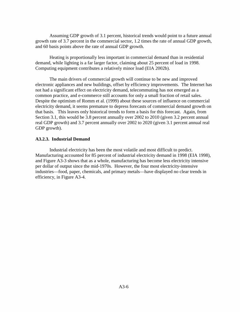
A3-6

Assuming GDP growth of 3.1 percent, historical trends would point to a future annualgrowth rate of 3.7 percent in the commercial sector, 1.2 times the rate of annual GDP growth,and 60 basis points above the rate of annual GDP growth.

Heating is proportionally less important in commercial demand than in residentialdemand, while lighting is a far larger factor, claiming about 25 percent of load in 1998.Computing equipment contributes a relatively minor load (EIA 2002b).

The main drivers of commercial growth will continue to be new and improvedelectronic appliances and new buildings, offset by efficiency improvements. The Internet hasnot had a significant effect on electricity demand, telecommuting has not emerged as acommon practice, and e-commerce still accounts for only a small fraction of retail sales.Despite the optimism of Romm et al. (1999) about these sources of influence on commercialelectricity demand, it seems premature to depress forecasts of commercial demand growth onthat basis. This leaves only historical trends to form a basis for this forecast. Again, fromSection 3.1, this would be 3.8 percent annually over 2002 to 2010 (given 3.2 percent annualreal GDP growth) and 3.7 percent annually over 2002 to 2020 (given 3.1 percent annual realGDP growth).

A3.2.3. Industrial Demand

Industrial electricity has been the most volatile and most difficult to predict.Manufacturing accounted for 85 percent of industrial electricity demand in 1998 (EIA 1998),and Figure A3-3 shows that as a whole, manufacturing has become less electricity intensiveper dollar of output since the mid-1970s. However, the four most electricity-intensiveindustries—food, paper, chemicals, and primary metals—have displayed no clear trends inefficiency, in Figure A3-4.

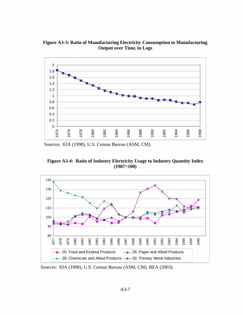
A3-7

Figure A3-3: Ratio of Manufacturing Electricity Consumption to ManufacturingOutput over Time, in Logs

0

0.2

0.4

0.6

0.8

1

1.2

1.4

1.6

1.8

2

1974

1976

1978

1980

1982

1984

1986

1988

1990

1992

1994

1996

1998

Sources: EIA (1998), U.S. Census Bureau (ASM, CM).

Figure A3-4: Ratio of Industry Electricity Usage to Industry Quantity Index(1987=100)

80

90

100

110

120

130

140

1977

1978

1979

1980

1981

1982

1983

1984

1985

1986

1987

1988

1989

1990

1991

1992

1993

1994

1995

1996

1998

20. Food and Kindred Products 26: Paper and Allied Products

28: Chemicals and Allied Products 33. Primary Metal Industries

Sources: EIA (1998), U.S. Census Bureau (ASM, CM), BEA (2003).

A3-8

Industrial demand for electricity will be affected not only by future rates of economicgrowth and energy efficiency advances of individual industries, but also by changes in thesectoral composition of production as well, and these are difficult to predict. Again lookingto historical trends, the percent of U.S. GDP deriving from manufacturing has been steadybetween 1987 and the recession year of 2001, fluctuating between only 16 and 17 percent(BEA 2003). Future trends of manufacturing electricity use may be influenced more bysectoral shifts than by reductions in the U.S. manufacturing base. For example, the output ofelectronics and other electronic equipment grew by nearly 14 percent a year from 1987 to2001, while that of total manufacturing averaged only about 2.5 percent a year. The high-technology industries are not especially electricity-intensive, but with continued pressurefrom overseas on traditional U.S. manufacturers, they may grow proportionally more in thecoming decades. Altogether, it may be difficult to improve on a projection of the 1992-2000trend of 1.2 percent annual growth of manufacturing electricity consumption growth to theperiod 2002 to 2020.

A3.3. Electricity Prices

Electricity prices may rise or fall in the future, but the response of consumption toprice changes is governed by the elasticity of demand for electricity. This section reviewseconometric studies of own-price elasticities for the residential. The literature’s generalconclusion on electricity is that it is a fairly price-inelastic good for the residential sector inthe short run but considerably more elastic in the long run. Cross-price elasticities areminimal because of the high equipment costs involved with switching fuels as well as theunavailability of natural gas and other alternative fuels in many areas.

The short-run elasticity measures the adjustment in the level of use of existingappliances that results immediately from a price change. The long-run elasticity alsoincorporates the change in electricity demand that results from changes in the appliance stockin longer-term adjustment to new prices. For thinking about electricity demand over adecade or more, the long-run elasticity is the more relevant measure.

The elasticity of residential electricity demand is a well studied parameterempirically, and estimates have varied considerably, as Table A3-1 shows. Following Bohi’s(1981) suggestion that aggregate data yielded biased estimates of electricity demandelasticities, Table A3-1 reports a number of studies estimating elasticities panel or cross-section data. Giving greater weight to more recent studies suggests a long-run elasticitybetween -0.50 and -1.0. NEMS uses a long-run residential own price elasticity of -0.31 in thelong run, and -0.25 for commercial demand (Wade 1999).

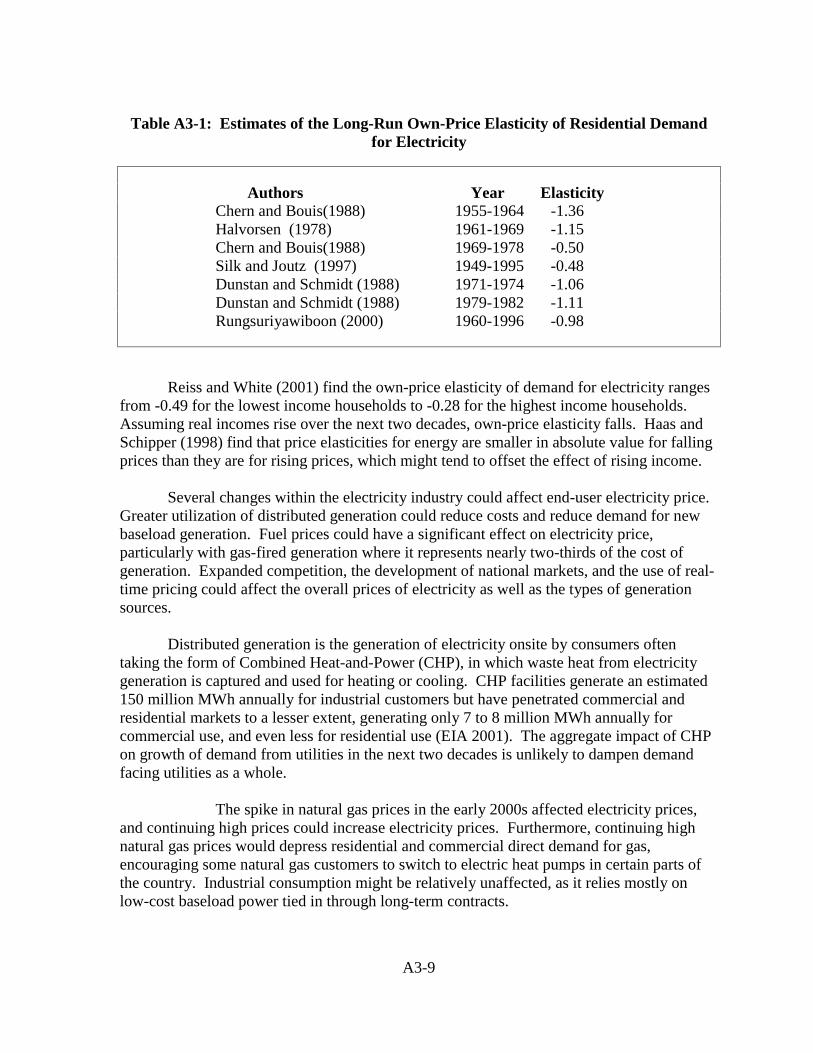
A3-9

Table A3-1: Estimates of the Long-Run Own-Price Elasticity of Residential Demandfor Electricity

Authors Year ElasticityChern and Bouis(1988) 1955-1964 -1.36Halvorsen (1978) 1961-1969 -1.15Chern and Bouis(1988) 1969-1978 -0.50Silk and Joutz (1997) 1949-1995 -0.48Dunstan and Schmidt (1988) 1971-1974 -1.06Dunstan and Schmidt (1988) 1979-1982 -1.11Rungsuriyawiboon (2000) 1960-1996 -0.98

Reiss and White (2001) find the own-price elasticity of demand for electricity rangesfrom -0.49 for the lowest income households to -0.28 for the highest income households.Assuming real incomes rise over the next two decades, own-price elasticity falls. Haas andSchipper (1998) find that price elasticities for energy are smaller in absolute value for fallingprices than they are for rising prices, which might tend to offset the effect of rising income.

Several changes within the electricity industry could affect end-user electricity price.Greater utilization of distributed generation could reduce costs and reduce demand for newbaseload generation. Fuel prices could have a significant effect on electricity price,particularly with gas-fired generation where it represents nearly two-thirds of the cost ofgeneration. Expanded competition, the development of national markets, and the use of real-time pricing could affect the overall prices of electricity as well as the types of generationsources.

Distributed generation is the generation of electricity onsite by consumers oftentaking the form of Combined Heat-and-Power (CHP), in which waste heat from electricitygeneration is captured and used for heating or cooling. CHP facilities generate an estimated150 million MWh annually for industrial customers but have penetrated commercial andresidential markets to a lesser extent, generating only 7 to 8 million MWh annually forcommercial use, and even less for residential use (EIA 2001). The aggregate impact of CHPon growth of demand from utilities in the next two decades is unlikely to dampen demandfacing utilities as a whole.

The spike in natural gas prices in the early 2000s affected electricity prices,and continuing high prices could increase electricity prices. Furthermore, continuing highnatural gas prices would depress residential and commercial direct demand for gas,encouraging some natural gas customers to switch to electric heat pumps in certain parts ofthe country. Industrial consumption might be relatively unaffected, as it relies mostly onlow-cost baseload power tied in through long-term contracts.

A3-10

Currently 22 states have implemented some form of deregulation for electricity.Assuming the trend toward deregulation picks back up, prices might be projected to fall. ThePolicy Office Electricity Modeling System (POEMS) model produced by DOE in 1998,projects the difference in electricity prices between regulated and deregulated markets by2010 at $63 per MWh versus $55 per MWh, as existing plants move to improve efficiencyand prices are bid down to marginal cost. At a long-run elasticity of demand for electricity of-1.0, that could lead to an increase in demand of nearly 15 percent, or by half that if theelasticity is -0.5.

Real-Time Pricing (RTP) is a mechanism to align customer and producer costs. Thecost of producing electricity varies with the demand for electricity throughout the day, risingparticularly in morning and late afternoon/early evening peaks. Charging consumers pricesthat reflect utilities’ generation costs during the course of the day would give them incentiveto shift some of their use of energy-intensive appliances to off-peak hours. While totalmegawatt hours might not be reduced significantly, widespread use of RTP could slow thegrowth of demand for new capacity.

Quantifying these effects is beyond the scope of this study, but the combination ofoffsetting influences they pose suggests that projection of historical trends in aggregateelectricity use could wash out many minor errors and not be wide of the mark.

A3.4. Future Demands for Additional Capacity at the National Level

This section forecasts a range of future time at which new capacity will be required inorder to meet national electricity demand. The first part of this section examines somecurrent projections; the second and third parts outline parameters used for forecasting; andthe last part presents projections for demand growth and time when new capacity will beneeded. Utilizing figures for current generating capacity, projections for plant retirements,and a range of possible demand growth rates, it is estimated that new capacity will not beneeded until 2015 at the aggregate level.

A3.4.1. NEMS Projections of Generation Capacity Growth

As a prelude to the projections presented in this section, it is important to review analready standard set of forecasts. EIA’s Annual Energy Outlook 2003 includes the results oftwo different scenario of electricity demand growth using the NEMS model. The first ispresented as a reference scenario based on an annual growth of 1.8 percent, while the otherassumes a high growth rate of 2.5 percent based on which electricity demand grows 2.5percent annually rather than the 1.8 percent produced in the reference scenario. Thesescenarios yield results of a 2.2 percent annual increase in generation capacity under the highdemand case and a 1.5 percent annual increase under the low demand case.

On closer examination, the results of the NEMS model seem to be at odds with thecurrent choices for new generation, being almost entirely made up of natural gas-fired plants.

A3-11

However, although natural gas has been the fuel of choice for new generation in the past,some new coal capacity announcements have been made recently. Several factors are likelyat work in the renewed interest in coal, including rising natural gas prices, looser federalregulations regarding environmental retrofits to coal plants, and the proposed new energybill, which offers incentives for coal as well as nuclear power.

A3.4.2. Current Generating Capacity and Demand

Currently, the United States has an over supply of generating capacity. As of October31, 2003, total national supply equaled 964,469 MW (Smith 2003). Using projections for netinternal demand for electricity during the summer of 2003 of 695,672 MW according to aJuly 2003 A.G. Edwards report (Fischer et al. 2003), and 716,728 MW according to the June2003 Merrill Lynch report, yields a calculated reserve margin between 28 percent and 29percent in 2003. Given the current amount of capacity, this will probably rise greater than30 percent in 2004. This is already far in excess of suggested reserve margins necessary forinvestment and operation: Fischer et al. (2003) report 18 percent as ideal for investment, andMerrill Lynch (2003a) supports 15 percent to be an equilibrium level. In addition to theselarge reserves, there is between 25,000 MW (Merrill Lynch 2003a estimate) and 36,000 MW(Fischer et al. 2003 estimate) of new capacity that is under construction now and will comeonline between 2004 and 2005. This brings the total generating capacity of the United Statesto approximately 950,000 MW by summer of 2005.

A3.4.3. Plant Retirements

Plant retirements may speed the need for new capacity, but the extent of possiblefuture retirements is difficult to discern. EIA, in the AEO 2003, estimates that 66,800 MWof capacity will be retired by 2010, with only 13,000 MW being retired by 2005, andvirtually all of the retired capacity coming from older oil and gas fired plants. Furthermore,environmental regulations may be enacted between now and 2020 which force older, morepolluting coal plants to shut down.

A3.4.4. Projections

Based on projections of electricity demand growth by sector presented earlier, thisappendix estimates a total annual demand growth rate of 2.6 percent, nearly 70 basis pointshigher than that projected by the EIA, and 80 basis points higher than that projected byGlobal Insight (Table A3-2).

A3-12

Table A3-2: Comparison of Forecasts of Electricity Demand Growth through 2020,Percent per Year

Historical(1980-2001)

EIA (AEO 2003)

GlobalInsight

ThisAppendix

Residential 2.5 1.7 2.1 2.6Commercial 3.7 2.2 2.0 3.7Industrial 1.0 1.7 2.0 1.2Total 2.3 1.9 1.8 2.6GDP Growth 3.1 3.1 3.1 3.1

Source: EIA (2003a).

Table A3-3 presents projections for new aggregated generating capacity that will beneeded for selected future years, given the different growth rate estimates from Table 3-2.These results are based on assumptions of a 15 percent reserve margin, a 2003 peak demandof 705,000 MW (the average of the two earlier estimates), current capacity total of 965,000MW in 2003, and capacity close to 1,000,000 MW by 2005 (due to the addition of capacityunder construction now).

Table A3-3: Estimations of Future Generating Capacity Needs

Projected Electricity Demand Growth, Percent per YearYear 1.80 1.90 2.30 2.602003 829,412 829,412 829,412 829,4122005 859,539 861,229 868,003 871,4012010 939,733 946,214 972,522 985,9102015 1,064,729 1,079,466 1,140,326 1,115,4672020 1,272,673 1,303,019 1,431,480 1,262,048

Source: EIA (2003a).

For every growth scenario, new capacity will not be needed until 2015 if existingcapacity stays close to its assumed 2005 value.

A3.5. Regional Projections of Demands for New Capacity

Section A3.7 estimates that the United States will not need new generation capacityuntil 2015 due to its current excess capacity. However, current excess capacity is not evenlydistributed across the country, with several regions having a tight supply even if the whole

A3-13

nation is over-supplied. Since, power currently cannot be easily shared across regions due tosignificant transmission constraints, projections of future capacity needs should bedifferentiated by region. This section analyzes the country by region, in order to get a bettersense of when capacity will be needed, how much, and where.

This section presents an analysis that applies projections of plant retirements anddifferent demand growth rates to figures for the amount of current stock in order to gaugefuture capacity needs by region. The date at which new capacity would be needed by eachregion is estimated given two different future demand scenarios, based on high and lowdemand growth rates estimates.

Capacity figures come partially from the equity research reports prepared by A.G.Edwards (Fischer et al. 2003), Morgan Stanley (2002, 2003a, 2003b), and Merrill Lynch(2003a, 2003b). Their projected reserve margins are based on the available resources ascalculated by the North American Electric Reliability Council (NERC) and found in Fischeret al. (2003), which concerns itself primarily with plant reliability. Therefore there is asignificant amount of capacity that does not get included, because it is not committed.Merrill Lynch makes an estimate of the actual capacity in several regions, where the actualcapacity is significantly higher than the reported capacity. Every effort has been made to usethe highest estimate of capacity, in order to most accurately reflect the amount of capacityactually in existence going forward, as that determines what more will be built.

The timing and location of plant retirements are primarily based on the NEMS model.NEMS tries to capture some of the various factors that contribute to decision for plantretirement, including environmental regulations, projected future electricity prices, andprojected future operating costs, and outputs an estimated timetable of type, timing, size, andlocation of retirements. Along with NEMS, A.G. Edwards’ table of gas/oil fired plants withheat rates of 12,000 BTUs and above (44,000 MW) is also used (Fischer et al. 2003). At thislevel of heat generation, it is impossible to operate a plant while still making a profit(Morgan Stanley 2003a, 2003b).

Region-specific demand growth rates are based on projections from NERC, EIA, andthose presented earlier in this appendix. The third set of growth rates is calculated byapplying the growth rates of demand estimated earlier in this paper to the shares of electricitydemanded by the residential, commercial, and industrial sectors in each region. From thisrange of estimates, two specific growth rates are chosen to model a high and a low demandgrowth scenario.

The model assumes a minimum capacity reserve margin of 15 percent. This is basedon historical observations: before the boom in new capacity starting in 2000-2001, reservemargins were in the 14 to 15 percent range in the United States during 1998-2000.

The effect of population shifts from region to region is not accounted for, though itcan implicitly be assumed that regions to the south and west will experience higher growththan those to the north and east.

A3-14

Table A3-4 reports projections of demand for new capacity for NERC regions underassumptions of high and low demand growth. The table identifies the year in which theamount of current capacity will fall short of total retirements in each region. For example, inthe first row, the ECAR region will need new capacity in 2010 under a high demand growthscenario but not until 2012 under a low demand growth scenario. Even under low demandgrowth, new capacity is needed in five of the eleven NERC regions by 2010. It is very safeto say that demands for new electricity generating capacity will be sufficient to justifysignificant amounts of new capacity by the year 2015, which is the year of new plantconstruction used in the analysis of viability of nuclear power in the present study.

Table A3-4: Years When New Capacity will be Needed, by NERC Region, with Highand Low Growth Rates of Electricity Demand

REGIONa 2005 2006 2007 2008 2009 2010 2011 2012 2013 2014 2015 2016 2017ECAR H LERCOT H LFRCC H LMAAC H LMAIN H LMAPP H LNEPOOL H LNYCA H LSERC H LSPP H LWECC H L

H= High Annual Demand Growth ProjectionL= Low Annual Demand Growth Projection

Source: NERC (2003).aNERC Region Definitions: ECAR, East Central Area Reliability: MI, IN, OH, KY, WV, small areas in PAand VA; ERCOT, Electric Reliability Council of Texas: most of Texas; FRCC, Florida ReliabilityCoordinating Council: most of Florida; MAAC, Mid-Atlantic Area Council: NJ, MD, DE, and most of PA;MAIN, Mid-America Interconnected Network: IL, most of WI, parts of MS, IA, MN; MAPP, Mid-ContinentArea Power Pool: ND, SD, NE, IA, parts of WI and MT; NEPOOL, New England Power Pool: CT, ME,MA, NH, RI, VA; NYCA, New York Control Area: NY; SERC, Southeastern Electric Reliability Council:VA, GA, LA, AR, MS, TN; SPP, Southwest Power Pool: KS, OK, small areas of AR, LA, NM; WECC,Western Electricity Coordinating Council: entire western US.

A3-15

A3.6. Conclusion

The United States, in the aggregate, has a large stock of excess power capacity, but itis, distributed unevenly among regions. This appendix presents some projections of futureelectricity capacity needs given a variety of demand and supply scenarios at the aggregatenational level and by region. For the nation as a whole, new capacity is not needed until2015 for low and high demand growth rate scenarios. However, most excess capacity islocated in the South, West, and Northeast, while other regions have much lower excesscapacities available presently. Five out of the eleven NERC regions would require newcapacity by 2010 even under projections of low demand growth. These areas include thefollowing states: Florida, New Jersey, Maryland, Delaware, Pennsylvania, Illinois, NewYork, and parts of Wisconsin and Montana. The last region to need new capacity will beSERC, the Southeastern Electric Reliability Council, which includes Virginia, Georgia,Louisiana, Arkansas, Mississippi, and Tennessee. SERC will not need to increase its currentcapacity until 2015 under a high demand growth scenario and 2017 under a low demandgrowth scenario.

A3-16

References

Bureau of Economic Analysis (BEA). (2003) U.S. Economic Accounts, National Incomeand Product Accounts Table (GDP). Washington, DC: U.S. Department of Commerce.Retrieved from the World Wide Web: http://www.bea.gov/bea/dn/nipaweb/.

Bureau of Labor Statistics (BLS). (2003) Current Population Survey (CPS). Washington,DC: U.S. Department of Labor. Retrieved from the World Wide Web:http://www.bls.gov/cps/.

Bohi, Douglas R. (1981) Analyzing Demand Behavior: A Study of Energy Elasticities,1st ed. Baltimore: Johns Hopkins University Press.

Chern, Wen S., and Howarth E. Bouis. (1988) “Structural Change in Residential EnergyDemand,” Energy Economics 10: 213-222.

Department of Energy, Office of Policy and International Affairs (DOE). (1998) PolicyOffice Electricity Modeling System (POEMS) documentation. Retrieved December 13, 2003from the World Wide Web: www.policy.energy.gov/electricity/appndxc.pdf.

Dunstan, Roger H., and Ronald H. Schmidt. (1988) “Structural Changes in ResidentialEnergy Demand,” Energy Economics 10: 206-212.

Energy Information Administration (EIA). (2003a) Annual Energy Outlook 2003 withProjections to 2025, DOE/EIA-0383. Washington, D.C.: U.S. Department of Energy,January 9, 2003.

Energy Information Administration (EIA). (2003b) Monthly Energy Review November 2003.Washington, D.C.: U.S. Department of Energy, November 24, 2003.

Energy Information Administration (EIA). (2003c) The National Energy Modeling System:An Overview 2003. Washington, D.C.: U.S. Department of Energy, March.

Energy Information Administration (EIA). (2003d) Short Term Energy Outlook-August2003. Washington, D.C.: U.S. Department of Energy, August.

Energy Information Administration (EIA). (2003e). Supplement Tables to the AnnualEnergy Outlook 2003. Washington, D.C.: U.S. Department of Energy.

Energy Information Administration (EIA). (2002a) Annual Energy Outlook ForecastEvaluation 2002. Washington, D.C.: U.S. Department of Energy, November 5, 2002.

Energy Information Administration (EIA). (2002b) Commercial Buildings EnergyConsumption Survey 1999 (CBECS). Washington, D.C.: U.S. Department of Energy, 2002.

A3-17

Energy Information Administration (EIA). (2001) Annual Energy Review 2001.Washington, D.C.: U.S. Department of Energy.

Energy Information Administration (EIA). (1999) Annual Energy Outlook 2000 withProjections to 2020. DOE/EIA-0383(2000). Washington, D.C.: U.S. Department of Energy,December 17, 1999.

Energy Information Administration (EIA). (1998) Manufacturing Energy ConsumptionSurvey 1998 (MECS). Washington, D.C.: U.S. Department of Energy, 1998.

Energy Information Administration (EIA). (1997) Residential Energy Consumption Survey1997 (RECS 1997). Washington, D.C.: U.S. Department of Energy.

Fischer, Douglas A., Timothy M. Winter, Charles J. Fishman, Michael Doyle, Neil A.Kalton, and Jose Ramon. (2003) Energy Power Supply/Demand Study. New York:A.G. Edwards, July 9.

Haas, Reinhard, and Lee Schipper. (1998) “Residential Energy Demand in OECD-Countries and the Role of Irreversible Efficiency Improvements,” Energy Economics 20: 443-461.

Halvorsen, Robert. (1978) Econometric Models of U.S. Energy Demand. Lexington: D.C.Heath and Company.

Koomey, Jonathan G., Richard E. Brown, Robert Richey, Francis X. Johnson, Alan H.Sanstad, and Leslie Shown. (1995) Residential Sector End-Use Forecasting with EPRI-REEPS 2.1: Summary Input Assumptions and Results. LBNL-34044. Berkeley: LawrenceBerkeley National Laboratory, December. Retrieved December 13, 2003 from the WorldWide Web: http://enduse.lbl.gov/Info/LBNL-34044.pdf.

Koopmans, Carl C., and Dirk Willem te Velde. (2001) “Bridging the Energy EfficiencyGap: Using Bottom-Up Information in a Top-Down Energy Demand Model,” EnergyEconomics 23: 57-75.

Merrill Lynch. (2003a) “Electric Utilities & IPPs.” New York: Merrill Lynch, June 12.

Merrill Lynch. (2003b) “Paper and Forest Products. Money can Grow on Trees.” NewYork: Merrill Lynch, July 14.

Merrill Lynch. (2002) “The Four Corners.” New York: Merrill Lynch, May 9.

Morgan Stanley. (2003a) The Power Meter-Unregulated Power Update. August 12.

Morgan Stanley. (2003b) The Power Meter-Unregulated Power Update. October 1.

A3-18

North American Electric Reliability Council. Description of Regional Reliability Councils.Retrieved from World Wide Web June 4, 2004: http://www.nerc.com/regional.

Reiss, Peter C., and Matthew W. White. (2001) “Household Electricity Demand, Revisited,”Cambridge, Mass.: National Bureau of Economic Research. Working Paper No. 8687.Retrieved December 12, 2003 from the World Wide Web: www.nber.org/papers/w8687.

Romm, Joseph, Arthur Rosenfeld, and Susan Herrman. (1999) The Internet Economy andGlobal Warming. The Center for Energy and Climate Solutions. Retrieved December 13,2003 from the World Wide Web: http://www.cool-companies.org/energy/ecomm.doc.

Rungsuriyawiboon, Supawat. (2000) “Demand for Residential Electricity in the UnitedStates,” Mimeo. Department of Energy, Environmental, and Mineral Economics. University Park, Penn.: Pennsylvania State University, May 5. Subsequently published as:Rungsuriyawiboon, S. (2002) “Estimating Residential Demand for Electricity in the UnitedStates.” Chiang Mai Journal of Economics, 6: 91-97.

Silk, Julian I., and Frederick L. Joutz. (1997) “Short and Long-Run Elasticities in U.S.Residential Electricity Demand: A Co-Integration Approach,” Energy Economics 19: 493-513.

Smith, Rebecca. (2003) “Electric Industry Capacity Glut Jolts Investors,” The Wall StreetJournal, November 11: A2.

U.S. Census Bureau. Annual Survey of Manufactures (ASM). 1972-1998. Washington, D.C.:U.S. Department of Commerce.

U.S. Census Bureau. Census of Manufactures (CM). 1977, 1982, 1987, 1992, 1997.Washington, D.C.: U.S. Department of Commerce.

Wade, Steven H. (1999) “Price Responsiveness in the NEMS Buildings Sector Models.”Energy Information Administration Issues in Midterm Analysis and Forecasting 1999.EIA/DOE-0607(99). Washington, D.C.: U.S. Department of Energy. Retrieved December15, 2003 from the World Wide Web:http://www.eia.doe.gov/oiaf/issues/building_sector.html.

A4-1

Appendix A4. TECHNOLOGIES FOR NEW NUCLEAR FACILITIES

Summary

The nuclear reactors currently in use in the United States, denoted as Generation II,were deployed in the 1970s and 1980s. These include boiling water reactors and pressurizedwater reactors. Advanced reactor designs, Generation III, have been developed in order to bemore cost competitive with natural gas. Generation III includes the advanced boiling waterreactor (ABWR) and the AP600 (pressurized water) passive-design reactor. The nuclearindustry has continued to develop yet more innovative designs designated Generation III+.Generation III+ includes a gas cooled reactor, the Pebble Bed Module (PBMR), as well as acapacity upgrade from AP600 to AP1000. Generation III+ may have even lower generatingcosts, however, the U.S. Nuclear Regulatory Commission (NRC) has not certified thesedesigns, and their cost estimates have greater uncertainty. The nuclear industry also hasplans for Generation IV technologies, but these reactor designs may not be available foranother two decades, and their cost estimates are even more uncertain.

The U.S. Department of Energy (DOE) has organized the Near Term DeploymentGroup (NTDG) to examine prospects for the deployment of new nuclear power plants in theUnited States over the next 10 years. Nuclear suppliers submitted eight plant designs forassessment. General Electric submitted designs for the ABWR as well as the EuropeanSimplified Boiling Water Reactor (ESBWR), and Westinghouse submitted designs for theAP600, AP1000, and the International Reactor Innovative and Secure Design (IRIS). TheIRIS is a modular light water reactor. Framatome ANP submitted a design for the SWR1000, a boiling water reactor (BWR) incorporating passive safety features. Eskom submitteda design for its PBMR design, and General Atomics provided NTDG its design for a GasTurbine Modular Helium Reactor (GT-MHR). The PBMR and GT-MHR are based on gasreactors built in Germany.

The ABWR is the only reactor type that has been built. Although never built, theAP600 has obtained design certification and boasts extensive verification of its costestimates. Like the ABWR it faces concerns with economic competitiveness. As a scaled-upversion of the AP600, the AP1000 should be more economically competitive, but is stillseeking design certification. Despite offering larger potential economic savings, the PBMRand GT-MHR are only in very preliminary stages, and major uncertainties are to be resolved.The IRIS project has perhaps the largest upside of the reactor types, but is not considered tobe a realistic option for near-term deployment. Framatome has opened discussion with NRCto obtain certification for the SWR 1000 in the United States. GE wants to commercializethe ABWR domestically prior to introducing the ESBWR to the U.S. market.

The best near-term candidates are the ABWR, the AP1000, the SWR 1000, and theCANDU ACR-700. The first three are ALWR designs, based on the PWR and BWR designsin operation in the United States. These PWR and BWR designs account for the greatmajority of reactors in operation throughout the world. The ALWR designs have acquireddesign certification. Unlike the gas cooled reactors, the ALWR designs have no design or

A4-2

engineering gaps to overcome. The ALWR has solid cost estimates based on actual buildingexperience. Expected learning curve cost reductions will improve the cost competitivenessof subsequent plants. The CANDU ACR-700 reactor is a light water-cooled, heavy water-moderated design, a closely related version of which, the CANDU 6, has had units builtrecently in China and a site’s second unit begun in Romania. The ACR-700 uses 75 percentless heavy water than the CANDU-6.

It is anticipated that the AP600’s design certification will simplify the certification forthe AP1000, but the AP600 still will not actually be built due to its smaller size. GE does nothave immediate plans to commercialize the ESBWR. The PBMR, GT-MHR, and IRIS planshave too much uncertainty to be reliable candidates for nuclear plant construction in theUnited States in the near term. In the longer term the advanced gas cooled reactors andgeneration IV designs may become viable alternatives. The EPR is a large pressurized waterreactor which the French Ministry of Industry is considering building as a demonstrationplant by 2010. The System 80+ received NRC design certification in 1997, and plants havebeen built in Korea using this design, but Westinghouse has not expressed an intention tomarket that design in the United States.

A4-3

Outline

A4.1. Introduction

A4.2. Overview of Nuclear Power Plant Designs

A4.2.1. Functions and Design Choices in Nuclear ReactorsA4.2.2. Nuclear Plant GenerationsA4.2.3. Nuclear Plant Types in OperationA4.2.4. Worldwide Nuclear Plant OperationA4.2.5. Nuclear Plants Under Construction

A4.3. Near-Term Deployment Design Criteria

A4.3.1. Regulatory AcceptanceA4.3.2. Industrial InfrastructureA4.3.3. Commercialization PlanA4.3.4. Cost Sharing PlanA4.3.5. Economic CompetitivenessA4.3.6. Fuel Cycle Industrial Structure

A4.4. Near-Term Candidates

A4.4.1. ABWRA4.4.2. AP1000A4.4.3. SWR 1000A4.4.4. CANDU, ACR-700A4.1.5. AP600A4.4.6. ESBWRA4.4.7. PBMRA4.4.8. GT-MHRA4.4.9. IRISA4.4.10. Other Candidates (not evaluated by NTDG)

A4.5. Evaluation of Near-Term Candidates

A4.5.1. ABWRA4.5.2. AP1000A4.5.3. SWR 1000A4.5.4. CANDU, ACR-700A4.5.5. AP600A4.5.6. ESBWRA4.5.7. PBMRA4.5.8. GT-MHRA4.5.9. IRISA4.5.10. Conclusion

References

A4-4

A4.1. Introduction

This appendix reviews near-term nuclear power plant technologies to set the stage forselecting reactor designs for economic analysis in Chapter 3. Section A4.2 offers anoverview of the generation of nuclear power plants, the array of nuclear technologies inoperation and currently under construction. Section A4.3 describes the criteria developed byU.S Department of Energy’s (DOE) Deployment Group (NTDG) for assessing the proximityof new reactor designs to commercialization. Section A4.4 briefly describes the majorcandidate reactors identified by the NTDG and Section A4.5 reports their scoring onNTDG’s assessment criteria. Section A4.6 concludes.

A4.2. Overview of Nuclear Power Plant Designs

To offer a context for the descriptions of the near-term reactor designs, the firstsection below describes the major functionalities of a nuclear power plant and the trade-offsinvolved in the technological choices within each major component. Generations of nuclearreactors, due to technical progress, are mentioned frequently in discussion of nuclear power.The second section describes the major generations. Then, types of nuclear plants inoperation are described. Two succeeding sections give figures on the nuclear plants inoperation worldwide and new reactor orders as well as domestic ownership of nuclear plants.This appendix culminates with a section on the advantages and disadvantages of the nuclearpower plant types, and the challenge for nuclear plant developers.

A4.2.1. Functions and Design Choices in Nuclear Reactors

The basic processes behind most nuclear power plants are similar to those in a coalplant: heat is generated, which produces steam, which in turn propels a steam turbine toproduce electricity. Gas plants use gas turbines rather than steam turbines, and some reactordesigns substitute a gas turbine for the steam production step. The most important differencebetween the coal and gas plants on the one hand and the nuclear plant on the other lies inhow heat is produced. Rather than burning coal, a nuclear plant splits uranium atoms. Toinduce fission, a Uranium-235 atom must absorb a free neutron, destabilizing the atom. Asthe atom begins to decay, it releases a large amount of heat energy and gamma radiation.Each absorption and fission event induces a second, setting in motion a chain reaction. Toincrease the probability of neutron absorption, it is often necessary to moderate the velocityof the free neutron. This has implications for reactor designs.

The three main forms of uranium are distinguished by their atomic weights. Whilethe most abundant form is Uranium-238, it cannot be induced to split like Uranium-235. Forthe purposes of electric power generation, uranium is commonly, but not always, enriched sothat it contains up to 3 percent Uranium-235, and is then formed into shapes appropriate forparticular reactor designs.

A4-5

In addition to material and construction differences among reactor vessels andcontainment structures, reactor designs differ in (1) the type of fuel they use, (2) how theymoderate neutron flow, and (3) how they manage the heat generated from the reaction. Fueltypes include natural unenriched uranium, enriched uranium, mixed thorium-uranium, andmixed-oxide fuels (MOX). Enrichment or fuel processing increases the overall cost of fuel,which leaves natural uranium the cheapest fuel. While neutron moderation is generallyrequired to increase the likelihood of neutron absorption by a U-235 atom, fuels that areenriched or have higher concentrations increase the probability of absorption, andconsequently require less moderation than other fuel types. Because of the processing costsinvolved in making them, moderators such as heavy water and graphite are considerablymore expensive than light water.

Several options exist for transforming the heat generated from nuclear reactions intoelectricity. In pressurized water reactors (PWRs), water is heated under pressure and sent toa heat exchanger to produce steam for the turbine. Alternatively, boiling water reactors(BWRs) utilize existing coolant water to generate steam, thereby reducing the chance for heatloss during its transfer. Reactors such as the CANDU use heavy water to transfer heatbecause it does not reduce the efficiency of the chain reaction by absorbing neutrons. Whileprevious CANDUs (CANDU-3, 6, and 9) used heavy water to transfer heat, the ACR-700uses light water to transfer heat and heavy water for moderation. Gas-cooled reactors utilizestable gases such as helium or carbon dioxide to act as a coolant because they have betterheat transfer properties than water. Finally, gas-cooled reactors such as the GT-MHR andPBMR employ a Brayton power cycle, which is the thermal expansion of gas to power a gasturbine, when they are used to generate electricity.

As with the relationship between fuel and moderator, there are trade-offs among heatmanagement techniques that result in differing costs and electricity production efficiencies.For example, a PWR requires that its coolant water be pressurized to 150 times atmosphericpressure to prevent it from boiling as it transfers heat to the power cycle, adding an extracost. Conversely, a BWR is a low-pressure design that directly produces steam for powergeneration, using its coolant water. However, its steam is contaminated with radionuclidesfrom contact with the reactor core, and these must be removed or shielded from the powercycle, reducing the cost savings from its low-pressure design. In another heat managementtechnique, gas turbines are more efficient producers of electricity than steam turbines,however their costs are higher and they require the use of helium, which is more expensivethan water. In sum, the array of current and future reactor designs (some of which aredescribed in Section A4.4) are essentially alternative combinations of fuel types, moderators,and the coolants and heat utilization techniques of heat management systems that attempt tomaximize the efficiency of electricity production while minimizing its cost.

The review of individual reactors in Section A4.4 emphasizes how each designrepresents a combination of these functions, as design choices trade off various physical andeconomic efficiencies.

A4-6

A4.2.2. Nuclear Plant Generations

DOE and the nuclear power industry categorize nuclear reactor designs according togenerations. Each generation incorporates evolutionary improvements with revolutionaryconcepts to take the next step in reactor technology. The first-generation reactors were theprototype commercial reactors of the 1950s and 1960s.

Generation II reactors were deployed in the 1970s and 1980s and are in commercialuse today. In the United States, they include such light-water reactors as the boiling waterreactor (BWR) and the pressurized water reactor (PWR), and, in Canada, the CANDU heavy-water reactor.

Referred to as advanced-design nuclear power plants, Generation III reactorsinclude the advanced boiling water reactor (ABWR), the ACR-700, the System 80+advanced pressurized water reactor (APWR), and the AP600 passive-design reactor. Thesedesigns were developed in the United States and certified by the U.S. Nuclear RegulatoryCommission in the 1990s. ABWRs and APWRs have been built and are in operation in othercountries around the world.

Generation III+ are reactors that can be deployed by 2010. They have been underdevelopment during the 1990s and are in various stages of design and implementation now.They include the pebble-bed modular reactor (PBMR) and the AP1000. Both have passivesafety features, and the PBMR is gas-cooled, two technological features that foreshadowGeneration IV reactors. The U.S. Nuclear Regulatory Commission (NRC) has not yetcertified these designs.

Generation IV reactors can be deployed by 2030, and are expected to be highlyeconomical, incorporate enhanced safety, produce minimal waste, and be impervious toproliferation. The International Reactor Innovative and Secure (IRIS) project reactor is theGeneration IV reactor furthest along in development. It is a light-water reactor (LWR)incorporating advanced engineering to increase safety and reduce operational costs. AnotherGeneration IV reactor is the gas turbine modular helium reactor (GT-MHR), which haspassive safety features and is gas-cooled.

DOE considers Generation III and III+ as candidates for near-term deployment. TheABWR is attractive because it has already been built overseas, and the AP600 has alreadyreceived design certification.

The Generation III+ models hold more promise economically, and the AP1000 isexpected to receive design certification by 2005. The PBMR may be more economical thanthe AP1000, but it needs substantially more development. The Generation IV reactors IRISand GT-MHR have the greatest potential for cost savings, but neither design will be availablefor near-term deployment to replace plants that are currently operational (NEI 2003).

A4-7

A4.2.3. Nuclear Plant Types in Operation

The pressurized water reactors (PWRs) and boiling water reactors (BWRs) are two ofthe most common designs worldwide (see Table A4-1). Moreover, the PWR and BWR arethe most common in the Americas and the only designs in operation in the United States.The United States has had over 70 PWRs and 40 BWRs in operation for several decades.

Table A4-1: Number and Power (in MW) of Reactors, by Type and Continent

Code Type Europe Africa Americas Asia TotalAGR Advanced Gas Cooled

Reactor14

(8,360)14

(8,360)BWR Boiling Water Reactor 20

(17,261)36

(31,639)34

(28,156)90

(77,056)FBR Fast Breeder Reactor 2

(793)2

(261)4

(1,054)GCR Gas Cooled Reactor 19

(3,125)19

(3,125)HWLWR Heavy-Water-

Moderated, Light-Water-Cooled

1(148)

1(148)

LWGR Light Water CooledGraphite Reactor

18(12,594)

18(12,594)

PHWR Pressurized HeavyWater Reactor

1(650)

22(14,436)

16(4,815)

39(20,001)

PWR Pressurized WaterReactor

109(106,560)

2(1,842)

71(65,917)

40(32,093)

222(206,412)

WWER Water Cooled WaterModerated PowerReactor

32(18,553)

1(376)

33(18,929)

Total 215(167,896)

2(1,842)

129(119,992)

94(65,849)

440(347,679)

Source: 2003 Power Reactor Information System (PRIS) database, IAEA (2003).

The Gas Cooled Reactor (GCR) is far less common, and no GCR is presently inoperation outside of Europe. Only two gas-cooled nuclear reactors have been operated in theUnited States, Peach Bottom-1 outside Philadelphia and the Ft. St. Vrain Plant in Platteville,Colorado, both of which were shut down after short periods of operation.

A4.2.4. Worldwide Nuclear Plant Operation

According to IAEA, there were 438 operating nuclear power plants worldwide at theend of 2001, with 353 GW of generating capacity. As of January 2002, the United States had104 reactors in operation, followed by France with 59, Japan with 54, the UK with 33, the

A4-8

Russian Federation with 30, and Germany with 19. Korea has increased deployment and had16 in operation. These countries were followed by Canada, India, Ukraine, Sweden, andSpain which had 14, 14, 13, 11, and 9 respectively. Eighteen other countries had six or fewerreactors in operation (IAEA 2000). As of January 1, 2003, there were 441 nuclear powerplants in operation with a total net installed capacity of 359 GW.

Six new nuclear plants were brought on line in Asian countries in 2002. They were:

• Qinshan 2-1, a 610 MW PWR in China

• Qinshan 3-1, a 655 MW PHWR in China

• Lingao 1, a 938 MW PWR in China

• Lingao 2, a 938 MW PWR in China

• Temelin 2, a 912 MW WWER in Czech Republic

• Yonggwang 6, a 950 MW PWR in Republic of Korea.

In the U.K., Bradwell units A and B, 123-MW GCRs were shut down in March 2002.In Bulgaria, Kozloduy 1 and 2 408-MW WWERs were shutdown in December 2002 (IAEAPRIS Database).

A4.2.5. Nuclear Plants Under Construction

The United States remains the leader in nuclear power generation, but that couldchange. Asian countries such as China, Japan, Korea, and India have been most active inbuilding new nuclear plants. Construction started on five additional nuclear power plants in2000__ one in China, two in India, and two in Japan. In 2001 construction began on anadditional reactor in Japan.

Altogether 32 nuclear plants were under construction worldwide at the end of 2001.China had eight under construction, Korea and Ukraine four, and Japan three. India, Iran, theRussian Federation, and Slovakia all had two under construction. Argentina, the CzechRepublic, and Romania had one under construction. As of January 1, 2003, 32 nuclearpower plants were under construction, with six new plants connected to the grid andconstruction beginning on seven new plants. Recently began construction is identifiedbelow:

• Kaiga 3, a 202 MW PHWR in India

• Kaiga 4, a 202 MW PHWR in India

• Rajasthan 5, a 202 MW PHWR in India

• Rajasthan 6, a 202 MW PHWR in India

• Kudankulam 1, a 905 MW WWER in India

A4-9

• Kudankulam 2, a 905 MW WWER in India

• LWR – Project Unit 1, a 1040 MW PWR in Dem. P. R. Korea.

A4.3. Near -Term Deployment Design Criteria

DOE has been working with the nuclear industry to establish a technical andregulatory foundation for the next generation of nuclear plants. DOE has organized a NearTerm Deployment Group (NTDG) to examine prospects for the deployment of new nuclearpower plants in the United States over the next 10 years. The NTDG established thefollowing six evaluation criteria as a basis for near-term deployment (DOE 2001).

A4.3.1. Regulatory Acceptance

Candidate technologies must show how they will be able to receive either aconstruction permit for a demonstration plant or a design certification by the U.S. NuclearRegulatory Commission (NRC) within the time frame required to permit plant operation by2010 or earlier.

A4.3.2. Industrial Infrastructure

Candidate technologies must be able to demonstrate that a credible set of componentsuppliers and engineering resources exist today, or that a credible plan exists to assemblethem, which would have the ability and the desire to supply the technology to a commercialmarket in the time frame leading to plant operation by 2010 or earlier.

A4.3.3. Commercialization Plan

A credible plan must be prepared which clearly shows how the technology would becommercialized by 2010 or earlier, including market projections, supplier arrangements, fuelsupply arrangements and industrial manufacturing capacity.

A4.3.4. Cost Sharing Plan

Technology plans must include a clear delineation of the cost categories to be fundedby government and the categories to be funded by private industry. The private/governmentfunding split for each of these categories must be shown, along with rationale for theproposed split.

A4.3.5. Economic Competitiveness

The economic competitiveness of candidate technologies must be clearlydemonstrable. The expected all-in cost of power produced is to be determined and comparedto existing competing technologies along with all relevant assumptions (includes plant capitalcost, first plant deployment cost, and other plant costs). Advanced passive designs are

A4-10

intended to reduce the costs of maintenance and operations testing while providing safetyimprovements.

A4.3.6. Fuel Cycle Industrial Structure

Candidate technologies must show how they will operate within credible fuel cycleindustrial structures. They must utilize a once-through fuel cycle with low-enriched uranium(LEU) fuel and demonstrate the existence of, or a credible plan for, an industrialinfrastructure to supply the fuel being proposed.

A4.4. Near -Term Candidates

The reactor designs considered in this appendix are those identified by the NTDG inresponse to the Request for Information (RFI) issued by DOE in April 2001. The intent ofthe NTDG evaluation was to determine those reactor technologies sufficiently mature indesign and licensing to support deployment in this decade, and to assess their respectiveadvantages, disadvantages and readiness for near-term deployment. Eleven plant designsreviewed by NTDG (DOE 2001) are summarized in Table A4-2.

A4.4.1. ABWR

General Electric (GE) developed the 1,350 MW Advanced Boiling Water Reactor(ABWR) in cooperation with the Tokyo Electric Power Company, Hitachi and Toshiba. Thereactor is water-cooled and moderated and utilizes enriched uranium fuel. The ABWRincorporates design features proven in many years of worldwide BWR operating experience,along with advanced features such as vessel-mounted reactor recirculation pumps, fine-motion control rod drives and a state-of-the-art digital, multiplexed, fiber-optic control andinstrumentation system.

The ABWR design was reviewed and certified by NRC in 1996, under the provisionsof 10 CFR Part 52. It is the only one of the reactor designs evaluated for near-termdeployment for which all engineering is complete and there is actual construction andoperating experience. Two ABWRs, Kashiwazaki-Kariwa Units 6 and 7, went intocommercial operation in Japan in 1996 and 1997, and are currently in their fifth cycle ofoperation. More recently, two ABWR units received regulatory approval and are now underconstruction in Taiwan. Because the ABWR has active safety features, operation andmaintenance costs would be incurred to maintain the reliability of its safety systems.

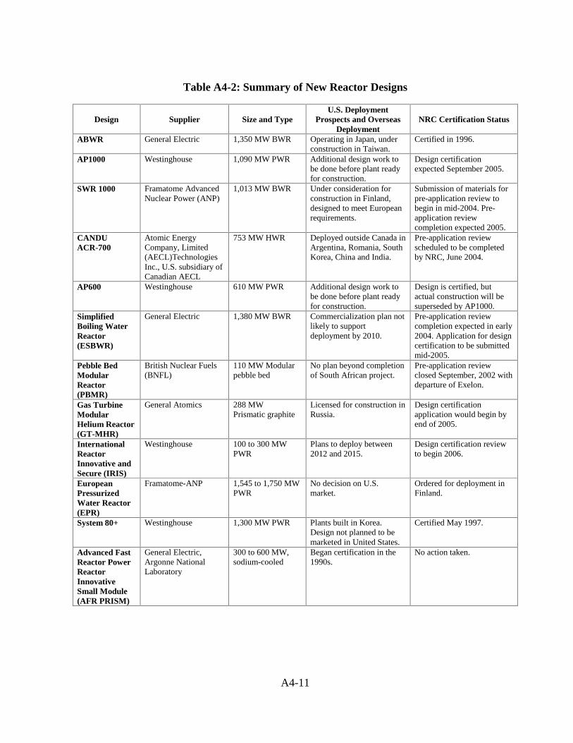
A4-11

Table A4-2: Summary of New Reactor Designs

Design Supplier Size and TypeU.S. Deployment

Prospects and OverseasDeployment

NRC Certification Status

ABWR General Electric 1,350 MW BWR Operating in Japan, underconstruction in Taiwan.

Certified in 1996.

AP1000 Westinghouse 1,090 MW PWR Additional design work tobe done before plant readyfor construction.

Design certificationexpected September 2005.

SWR 1000 Framatome AdvancedNuclear Power (ANP)

1,013 MW BWR Under consideration forconstruction in Finland,designed to meet Europeanrequirements.

Submission of materials forpre-application review tobegin in mid-2004. Pre-application reviewcompletion expected 2005.

CANDUACR-700

Atomic EnergyCompany, Limited(AECL)TechnologiesInc., U.S. subsidiary ofCanadian AECL

753 MW HWR Deployed outside Canada inArgentina, Romania, SouthKorea, China and India.

Pre-application reviewscheduled to be completedby NRC, June 2004.

AP600 Westinghouse 610 MW PWR Additional design work tobe done before plant readyfor construction.

Design is certified, butactual construction will besuperseded by AP1000.

SimplifiedBoiling WaterReactor(ESBWR)

General Electric 1,380 MW BWR Commercialization plan notlikely to supportdeployment by 2010.

Pre-application reviewcompletion expected in early2004. Application for designcertification to be submittedmid-2005.

Pebble BedModularReactor(PBMR)

British Nuclear Fuels(BNFL)

110 MW Modularpebble bed

No plan beyond completionof South African project.

Pre-application reviewclosed September, 2002 withdeparture of Exelon.

Gas TurbineModularHelium Reactor(GT-MHR)

General Atomics 288 MWPrismatic graphite

Licensed for construction inRussia.

Design certificationapplication would begin byend of 2005.

InternationalReactorInnovative andSecure (IRIS)

Westinghouse 100 to 300 MWPWR

Plans to deploy between2012 and 2015.

Design certification reviewto begin 2006.

EuropeanPressurizedWater Reactor(EPR)

Framatome-ANP 1,545 to 1,750 MWPWR

No decision on U.S.market.

Ordered for deployment inFinland.

System 80+ Westinghouse 1,300 MW PWR Plants built in Korea.Design not planned to bemarketed in United States.

Certified May 1997.

Advanced FastReactor PowerReactorInnovativeSmall Module(AFR PRISM)

General Electric,Argonne NationalLaboratory

300 to 600 MW,sodium-cooled

Began certification in the1990s.

No action taken.

A4-12

A4.4.2. AP1000

The AP1000 is a 1,090 MW PWR of the same basic design as the AP600, but up-rated in power to achieve economies of scale. The reactor is water-cooled and moderatedand utilizes enriched uranium fuel. The AP1000 passive safety systems are essentially thesame as those for the AP600, except for some changes in component capacities. The powerup-rate has been achieved by increasing the length and number of fuel assemblies, the size ofthe reactor vessel and primary components, and by increasing the height of the containmentstructure, and the size and capacity of the secondary plant energy conversion components.

The AP1000 generating cost is estimated to be 30 percent less than that of AP600because the additional power rating is achieved with a only a small increase in capital cost.AP1000 application for design certification was submitted to NRC in March 2002. NRCissued its draft safety report to Westinghouse in June 2003. A final safety evaluation isscheduled for issuance in September 2004, and the design certification rulemaking inDecember 2005 (NRC 2003). As with the AP600, additional detailed design work must alsobe done before the plant will be ready for construction.

A4.4.3. SWR 1000

SWR 1000 is a 1,013 MW BWR developed by Framatome Advanced Nuclear Power(F-ANP) in conjunction with German electric utility companies and European partners. TheSWR 1000 design combines proven, conventional BWR features with passive safety featuresto provide enhanced safety benefits. The plant is designed to meet European requirements,including relevant requirements in German nuclear codes and standards and otherrecommendations proposed by German and French reactor safety commissions for theEuropean Pressurized Water Reactor (EPR).

A four-year design phase for the SWR 1000 was completed in 1999, and included thedevelopment of a site-independent safety analysis report, a probabilistic safety analysisreport, and projected construction costs. In March 2003, Framatome submitted the SWR1000 design, along with the EPR, a pressurized water reactor to the Finnish power agency,Teollisuuden Voima Oy (TVO), for the fifth Finnish nuclear power plant. Presently no otherdesigns appear to be under consideration for this project. F-ANP advises that in parallel withefforts to market the SWR 1000 in Europe, they may consider entering the U.S. market.F-ANP met twice in 2002 with NRC to discuss submittal of the SWR 1000 for designcertification and have conveyed the intention to submit pre-certification material by mid-2004 (Cushing 2002, NRC 2002, Mallay 2002, Sebrosky 2002).

A4.4.4. CANDU, ACR-700

Canada’s current fleet of CANDU 3, 6, and 9 nuclear units are distinctive in their useof natural uranium fuel with online fueling. The CANDU 3, 6, and 9 nuclear units also haveheavy water coolant and moderation. The ACR-700 is likewise unique in that it uses 2.1percent enriched fuel and continues with online fueling, resulting in less expensive fuel costs

A4-13

than that for LWRs. The ACR-700 uses light water for cooling and heavy water formoderation. The ACR-700 uses 75 percent less heavy water than the earlier CANDU 3, 6,and 9 nuclear units. The ACR-700 reactor assembly is 30 percent smaller than that of theCANDU 3, 6, and 9 nuclear units. Combined with significant previous constructionexperience, simplification of the design and extensive use of modular construction arethought to greatly improve the ACR-700’s economic competitiveness in electric powergeneration.

CANDU reactors have been deployed outside Canada in Argentina, India, Romania,and South Korea, which opted in 2001 to continue its nuclear power expansion with1,000 MW units from Combustion Engineering rather than with CANDUs (NuclearEngineering International 2001). A 728 MW CANDU 6 unit was brought to full power atChina’s Qinshan site in November 2002, and a second unit was brought on line in July 2003,with a construction period of 51 months from the first pouring of concrete to criticality(AECL 2002, AECL 2003b, Hedges 2002, p. 8). AECL began construction on a second 710MW CANDU 6 unit at Cernavoda, Romania in April 2003, projecting a 48-monthconstruction period and an overnight cost of U.S. $700 million (AECL 2003a). AtomicEnergy of Canada, Limited (AECL), the CANDU’s vendor, requested pre-application reviewby NRC of its 700-MW ACR-700 design in June 2002, and NRC expects to complete its pre-application review in mid-2004 (Van Adel 2002; AECL Technologies 2002, p. 14; NRC2004, p. 2).

A4.4.5. AP600

The AP600 is a 610 MW PWR. The core, reactor vessel, internals, and fuel areessentially the same design as for presently operating Westinghouse PWRs. Fuel powerdensity has been decreased to provide more thermal margin. Canned rotor primary pumps,proven in the U.S. Navy’s reactor program and in fossil boiler circulation systems, have beenadopted to improve reliability and maintenance requirements.

The innovative aspect of the AP600 design is its reliance on passive features foremergency cooling of the reactor and containment, provided by natural forces such asgravity, natural circulation, convection, evaporation, and condensation, rather than on ACpower supplies and motor-driven components. Extensive testing of the AP600 passivecooling systems has been completed and supported by independent confirmatory testing byNRC to verify the design and analyses of the passive emergency cooling features. NRC hascertified the AP600 design. Additional detailed design work would be needed before theplant would be ready for construction. However, the thermal economics of the AP1000 aresuperior to those of the AP600, and it is considered unlikely that the AP600 will actually bedeployed, although its design certification may speed certification of the AP1000.

A4.4.6. ESBWR

The European Simplified Boiling Water Reactor (ESBWR) is a 1,380 MW, naturalcirculation, passively safe boiling water reactor developed by GE, in concert with

A4-14

international utilities, designers and research organizations. The design is based on the670 MW passively safe SBWR, initially developed in the early 1990s with DOE support, andit utilizes many design features of the ABWR.

The substantially higher plant power, combined with extensive simplification of thereactor systems and containment structure, allow significant cost reduction in comparisonwith both SBWR and ABWR. Although the ESBWR offers attractive advantages, GE is notyet moving ahead with detailed engineering and design certification of the plant. GE’scurrent plan is to proceed with ESBWR in a step-wise fashion, first with design certification,as funding becomes available, and then with detailed engineering, but only with thecommitment and financial support of a plant customer.

A4.4.7. PBMR

The Pebble Bed Modular Reactor (PBMR) is a 110 MW graphite-moderated, helium-cooled reactor. Heat generated by nuclear fission in the reactor is transferred to the heliumand converted into electrical energy in a gas turbine generator via a Brayton power cycle.The PBMR core is based on the German high temperature gas cooled technology and usesspherical fuel elements. The fundamental objective of the gas-cooled reactor design conceptis to achieve an exceptional level of nuclear safety, via fuel design that effectively precludesthe possibility of a core melt accident.

The PBMR helium gas passes through the reactor over the fuel pebbles, is heated, andthen flows directly through the turbine. This power conversion unit eliminates therequirement for a heat exchanger between a primary and secondary cycle, which improvesthe efficiency of the plant. The turbines that are used in light water reactors operate withlow-temperature and low-pressure steam.

PBMRs also refuel while in operation. New or reusable fuel pebbles are continuallybeing added to the reactor core from the top and removed from the bottom to measure howmuch fissile material is left. Each fuel cycle lasts about three months, with each fuel pebblepassing through the reactor about 10 times. A fuel sphere will last about three years and agraphite sphere about 13 years.

The first PBMR is planned for construction in South Africa, under a joint venture ledby Eskom. The plant design is currently in the detailed engineering stage and has recentlyreceived a record of decision (ROD) by the South African government to begin constructionof a demonstration module (Bennett 2003). Exelon, the largest nuclear utility in the UnitedStates, was an original member of the project and had planned to buy up to 40 modules, buthas since pulled out of the project as a result of change of business focus away from nuclearpower (Chalmers 2002). The pre-application design certification process for PMBR is nowno longer active.

A4-15

A4.4.8. GT-MHR

The Gas Turbine Modular Helium Reactor (GT-MHR) is a graphite-moderatedhelium cooled reactor. Each unit generates 288 MW, with up to four units comprising acomplete plant. Heat generated by nuclear fission in the reactor is transferred to the coolantgas (helium) and converted into electrical energy in a gas turbine generator. The fuelconsists of spherical fuel particles, each encapsulated in multiple coating layers, formed intocylindrical fuel compacts and loaded into fuel channels in graphite blocks.

The GT-MHR design offers very high thermal efficiency (approximately 48 percent)and outstanding nuclear safety. The GT-MHR is being developed under an internationalprogram in Russia for the disposition of surplus weapons plutonium. Government andprivate sector organizations from the United States, Russia, France, and Japan are sponsoringthe development work.

General Atomics (GA) has the lead responsibility for providing U.S. technicalsupport. The Russian GT-MHR demonstration plant is planned to be operational in 2009. Aparallel GT-MHR commercial plan has been assembled and could lead to adaptation of thedesign to utilize uranium fuel. The detailed design produced in Russia would be converted toU.S. standards and revised as necessary for the U.S. application. At this point, GA is activelyseeking a U.S. owner/operator. Although the United States has limited experience with GCRtechnology, much was learned from the 330 MW Fort St. Vrain Plant that has proven usefulin the continued development of the GT-MHR. Built by General Atomics (GA) as a DOEdemonstration plant in 1973, Fort St. Vrain was transferred in 1979 to Public ServiceCompany of Colorado and operated for several years before being shut down in 1989, afterexperiencing technical problems, particularly intrusion of moisture from water-cooledbearings. The GA-built helium-cooled reactor operated at 1,400 degrees Fahrenheit andproduced 330 MW of electricity. Despite operation and maintenance difficulties, the hightemperature plant demonstrated enhanced safety characteristics, including significantlyreduced radiation exposure to its workforce, and the use of hexagonal prismatic fuel blocks,which have continued to be used in the GT-MHR (Margolis 2003). Moreover, the plant waslauded as the first successfully decommissioned nuclear plant in 1996 (Nuclear EnergyInsight 1997, p. 4). The plant has since been repowered as a combined-cycle gas turbineplant producing near 720 MW of electricity.

A4.4.9. IRIS

IRIS is an innovative small (100 to 300 MW) pressurized water reactor underdevelopment by Westinghouse. The key feature of the IRIS design is the integrated primarysystem, that is, all primary system components, including the steam generators, coolantpumps and pressurizer, are housed along with the nuclear fuel in a single, large pressurevessel. As such, IRIS offers potential safety advantages, primarily related to the eliminationof any potential for large-break loss of coolant accident. Its small size and modular designmay simplify on-site construction and make it deployable in areas not suitable for largenuclear plants.

A4-16

IRIS is currently in the conceptual engineering stage and is being developed by aninternational consortium, with some support from DOE via the Nuclear Energy ResearchInitiative (NERI) Program. However, the integral primary system configuration introducessignificant design and licensing challenges that will be difficult to overcome, particularly inthe relatively short time frame established for near-term deployment. In key design details,IRIS is fundamentally different from any reactor licensed and operating in the United States.For that reason, extensive analysis and testing will be needed as a prerequisite to NRClicensing and commercial deployment in the United States. The IRIS sponsors’ response tothe NTDG RFI identifies this needed development and testing.

A4.4.10. Other Candidates (not evaluated by NTDG)

The NTDG evaluated those candidate reactor designs submitted per the requirementsof the DOE Request for Information, as described above. For completeness, it is noted thatother designs may also be deployable by 2010. However, these were not evaluated, and theNTDG offers no judgment as to their feasibility as near-term deployment candidates.

A4.4.10.1. EPR

The European Pressurized water Reactor (EPR) is a very large (1,545 MW or 1,750MW) design developed in the 1990s as a joint venture by French and German companies,Framatome and Siemens. The basic design was completed in 1997, working in collaborationwith other European nations, and conforms to French and German laws and regulations.

As the EPR design was being developed, there was substantial cooperation betweenthe European utilities developing EPR user requirements and the U.S. utilities leading theU.S. ALWR Program and its Utility Requirements Document. The EPR was not submittedto the NTDG in time to support an assessment. Further, as with the SWR 1000, the designer,Framatome ANP, has not made a decision regarding entry into the U.S. nuclear market. TheFrench Ministry of Industry is considering building a demonstration plant by 2010 (AFP2003).

A4.4.10.2. System 80+

The System 80+ is a 1,350 MW PWR design developed by ABB-CE (now mergedwith Westinghouse). It conforms to the ALWR Utility Requirements Document and wascertified by NRC in May 1997. Plants based on the System 80+ design have been built inKorea. However, as of this time Westinghouse has chosen not to market the System 80+design in the United States.

A4-17

A4.4.10.3. AFR and the PRISM

The Advanced Fast Reactor (AFR) and the Power Reactor Innovative Small Module(PRISM) are two Generation IV designs that utilize a fast neutron spectrum and sodiumcooling for the purpose of creating a more closed fuel cycle. The use of the fast neutronspectrum allows the reactor to consume plutonium and other transuranic elements, therebyeliminating the need for additional disposal methods. The AFR is being developed toincorporate pyroprocessing that separates the fission products and re-fabricates fuel with theremaining uranium and transuranic products. The reactors range in size from 300 to 465MW per module. Argonne National Laboratory and General Electric are working on thisdesign (Roglans-Ribas et al. 2003; Boardman et al. 2000; Boardman, Dubberley, and Hui2000).

A4.5. Evaluation of Near -Term Candidates

The following sections summarize the NTDG evaluation of the eight-candidatereactor designs (DOE 2001). These include assessment of each candidate’s compliance withthe six criteria established by the NTDG, identified design-specific gaps, projected costperformance, schedule considerations, and overall potential for deployment by 2010. In eachof these evaluation categories, the NTDG conclusions for all eight candidates aresummarized in tabular form. The NTDG did not evaluate the ACR-700, so the summary forthat reactor is derived from the present study.

Tabular summaries are intended to provide a concise comparison of the relativemerits and demerits of the reactor designs evaluated. The NTDG evaluation of the degree towhich each of the candidate reactor designs meets the intent of the six criteria for near-termdeployment is summarized below. The NTDG judgments in each case were based on theinformation submitted by the respondent, on additional information provided (includingpresentations at NTDG meetings) and on the experience and judgment of the NTDG teammembers.

A4.5.1. ABWR

• Regulatory Acceptance: Meets criterion. Design is NRC certified.• Industrial Infrastructure: Meets criterion. International infrastructure exists and

has been demonstrated on Asian ABWR projects.• Commercialization Plan: Can meet criterion. ABWR has been successfully

commercialized in Japan and Taiwan.• Cost Sharing Plan: Meets criterion. No design-specific government funding

requested.• Economic Competitiveness: Can meet criterion. ABWR costs have high certainty

(based on actual experience), but U.S. economic competitiveness is uncertain becauseof relatively high capital cost; ABWR may be competitive in some market scenarios.

A4-18

• Fuel Cycle Industrial Structure: Meets criterion. ABWR utilizes conventional fuelof proven design.

• Design Specific Gaps: Economic competitiveness under some scenarios.

A4.5.2. AP1000

• Regulatory Acceptance: Pre-application steps are in process.• Industrial Infrastructure: Meets criterion. Strong infrastructure is in place.• Commercialization Plan: Can meet criterion, but require substantial financial

investment to complete the detailed design.• Cost Sharing Plan: Meets criterion. The Westinghouse plan proposes cost sharing

and supporting rationale for design certification and detailed design.• Economic Competitiveness: Meets criterion. AP1000 would be competitive in

today’s market.• Fuel Cycle Industrial Structure: Meets criterion. AP1000 will utilize conventional

nuclear fuel.• Design Specific Gaps: Design Certification; financial support for completion of

detailed design.

A4.5.3. SWR 1000

• Regulatory Acceptance: Can meet criterion. SWR 1000 design developed to meetEuropean requirements; translation/revision to U.S. requirements will be difficult butcould be achieved in time for 2010 deployment if initiated very soon.

• Industrial Infrastructure: Meets criterion. Strong infrastructure is in place.• Commercialization Plan: Indeterminate. Plan not provided; SWR 1000

commercialization in the United States is contingent upon F-ANP decision.• Cost Sharing Plan: Indeterminate. Cost sharing requested for design certification

only (source and amount of funding to complete first-time engineering not identified.)• Economic Competitiveness: Can meet criterion. Projected costs are attractive, but

they are highly uncertain, particularly under U.S. conditions.• Fuel Cycle Industrial Structure: SWR 1000 will utilize new fuel assembly design,

but requires development and qualification.• Design Specific Gaps: Commitment by Framatome ANP; licensing to U.S.

regulatory and industry standards.

A4.5.4. CANDU, ACR-700

• Regulatory Acceptance: Pre-application review was requested June 19, 2002, and isexpected to be completed in 2004.

• Industrial Infrastructure: Several similar plants (CANDU 6 units) have beencompleted recently or are under construction in China, Korea, and Romania.

A4-19

• Commercialization Plan: Can meet criterion. The ACR-700 is an evolution of theproven CANDU-6 units, of which the last six have been built on or ahead of scheduleand on budget.

• Cost Sharing Plan: Meets criterion. The AECL plan does not request any specificfunding for design certification, only for NRC fees.

• Economic Competitiveness: AECL reports short lead times and low capital costs fortwin 700 MW units.

• Fuel Cycle Industrial Structure: Utilizes slightly enriched uranium (SEU) and aonce through fuel cycle.

• Design Specific Gaps: Achieving Design Certification; meeting all U.S.requirements.

A4.5.5. AP600

• Regulatory Acceptance: Meets criterion. Design is NRC certified.• Industrial Infrastructure: Meets criterion. Strong infrastructure is in place.• Commercialization Plan: Can meet criterion, but require substantial financial

investment to complete the detailed design.• Cost Sharing Plan: Meets criterion. The Westinghouse plan proposes cost sharing

and supporting rationale for design certification and detailed design.• Economic Competitiveness: Can meet criterion. Because of smaller capacity, has

higher capital and operating costs than AP1000. Based on Westinghouse projectedcosts, AP-600 may be competitive in some U.S. market scenarios.

• Fuel Cycle Industrial Structure: Meets criterion. AP600 will utilize conventionalnuclear fuel.

• Design Specific Gaps: Financial support for completion of detailed design; economiccompetitiveness under some scenarios.

A4.5.6. ESBWR

• Regulatory Acceptance: Can meet criterion. ESBWR design incorporates ABWRand SBWR design features, both previously reviewed by NRC.

• Industrial Infrastructure: Meets criterion. Same international infrastructure asdemonstrated on Asian ABWR projects would support ESBWR.

• Commercialization Plan: Does not meet criterion. ESBWR commercialization planis predicated on prior successful commercialization of ABWR. Therefore it is notlikely to support deployment by 2010.

• Cost Sharing Plan: Meets criterion. Cost sharing requested for design certificationand detailed design.

• Economic Competitiveness: Can meet criterion. GE did not provide costprojections; however, based on GE design economic targets and GE preliminaryestimates of material quantities, ESBWR would likely be economically competitive.

A4-20

• Fuel Cycle Industrial Structure: Meets criterion. ESBWR utilizes conventionalfuel of proven design (same fuel as ABWR).

• Design Specific Gaps: Design certification and completion of detailed design.

A4.5.7. PBMR

• Regulatory Acceptance: Can meet criterion, provided that several challengingtechnical issues (including fuel issues) can be resolved and demonstrated to NRCsatisfaction in the time frame needed for 2010 deployment. U.S licensing submittalinformation must be adapted from the German / South African design and test work.Pre-application steps with NRC are in progress.

• Industrial Infrastructure: Can meet criterion. International team is beingassembled. Design contracts are in place for major equipment.

• Commercialization Plan: PBMR had a potential U.S. customer (Exelon) with asubstantial initial commitment; however, Exelon has since changed its focus awayfrom further nuclear development and pulled out of the project. As such, nocommercialization plan beyond completion of the South African project exists.

• Cost Sharing Plan: Meets criterion. Proposed government cost sharing is primarilyfor licensing activities, including NRC confirmatory fuel characterization and testprograms.

• Economic Competitiveness: Can meet criterion. However, projected PBMReconomics are preliminary and have high uncertainty. Satisfactory economics rely ondeployment of multiple modules and successful development of the design.

• Fuel Cycle Industrial Structure: Can meet criterion. PBMR safety and reliabilityhinge on successful fuel development and high quality fuel manufacture. Currentplan includes ambitious program to develop, test, license and produce PBMR fuel,and presumes that initial U.S. fuel loads will be procured from a foreign supplier.

• Design Specific Gaps: Commercialization plan is uncertain given the recentwithdrawal by Exelon; fuel development, characterization, manufacture, testing andregulatory acceptance; performance of in-reactor high temperature materials; powerconversion system uncertainties with respect to components, ��������������������� �

A4.5.8. GT-MHR

• Regulatory Acceptance: Can meet criterion, provided that several challengingtechnical issues (including fuel issues) can be resolved and demonstrated to NRCsatisfaction in the time frame needed for 2010 deployment. U.S licensing submittalinformation must be adapted from the Russian design and test work.

• Industrial Infrastructure: Can meet criterion, provided that the Russian industrialinfrastructure can be qualified as a commercial supplier in the United States. Thismay be difficult to achieve in the time frame required for deployment by 2010.

• Commercialization Plan: Can meet criterion. However, this presumes continuedU.S. government support to the Russian project, timely identification of U.S.customer and industry partners, and technical success with Russian project.

A4-21

• Cost Sharing Plan: Meets criterion. Cost share proposal is predicated on continuedU.S. Government support to Russian project and presumes substantial private sectorparticipation for commercialization.

• Economic Competitiveness: Can meet criterion. However, projected GT MHReconomics are preliminary and have high uncertainty. Satisfactory economics rely ondeployment of multiple modules and successful development of the design.

• Fuel Cycle Industrial Structure: Can meet criterion. GT MHR safety andreliability hinge on successful fuel development and high quality fuel manufacture.Current plan includes ambitious program to develop, test, license and produce GTMHR fuel.

• Design Specific Gaps: Conversion of Russian prototype information and analyses,into����������������������������������������������������������������project; fuel development, characterization, manufacture, testing and ��������� acceptance; performance of in-reactor high temperature materials; power conversionsystem uncertainties with respect to components,��������������������� �

A4.5.9. IRIS

• Regulatory Acceptance: Does not meet criterion. Design certification in time for2010 deployment is unlikely, because of extensive analysis and testing required.

• Industrial Infrastructure: Can meet criterion. International IRIS design team,which includes manufacturing capability, has been assembled.

• Commercialization Plan: Does not meet criterion. Commercialization plan (in timeto support 2010 deployment) is unrealistic.

• Cost Sharing Plan: Meets criterion. Identified cost sharing would support IRISengineering, testing and licensing.

• Economic Competitiveness: Indeterminate. Westinghouse projections on IRIS costsare highly conjectural; if true, IRIS would be economically competitive, but there isnot yet a sufficient basis for confidence.

• Fuel Cycle Industrial Structure: Meets criterion, for initial fuel loads. However,more highly enriched fuel loads, intended for later years, would require newmanufacturing capability.

• Design Specific Gaps: Steam generator design, control, and accessibility forinspection as well as maintenance; integrated system safety performance, includingtransient response as well as primary system/containment interaction; internal controlrod drive mechanism (CRDM) development (and/or adequacy of conventionalCRDMs with long drive trains).

A4.5.10. Conclusion

The ABWR, the AP600, the AP1000, ACR-700 and the SWR 1000 are the onlyreactor types where the vendors appear willing and potentially able to meet the NTDGcriteria. The ABWR has design certification and is the only reactor type that has been built,

A4-22

but it still faces difficulty with economic competitiveness. The AP600 also has obtaineddesign certification, but it has been superseded by the AP1000 and probably will not be built.As a scaled-up version of the AP600, the AP1000 should be more economically competitive,but it also needs to finance a detailed design and it is has not yet obtained designcertification. The SWR 1000 appears to be the leading candidate for a project in Finland, andFramatome has met with NRC about obtaining design certification for the U.S. market.

GE wants to commercialize the ABWR domestically prior to introducing the ESBWRto the U.S. market. The remaining designs will not be able to satisfy the NTDG criteria sincethey are only in very preliminary stages and major uncertainties need to be resolved. ThePBMR must still test fuel integrity and high temperature materials.

Eskom’s plan to commercialize the PBMR has come under doubt since Exelondecided to withdraw from the project. The GT-MHR also needs to test fuel integrity andhigh temperature materials. Its prototype information has not been suitably documented byGeneral Atomics to submit an application for design certification. Finally, the IRIS projectstill requires extensive testing of its steam generator design and control. The project mustalso demonstrate that its steam generators will be accessible for inspection as well asmaintenance.

A4-23

References

AECL Technologies, Inc. (AECL Technologies). (2002) “A Plan for the Pre-ApplicationReview of the Advanced CANDU Reactor (ACR) (September 26, 2002). Mimeo, issued fordiscussion with NRC. Gaithersburg, Md.: AECL Technologies, Inc., September 26.

Atomic Energy of Canada, Ltd. (AECL). (2002) News release: “AECL’s CANDU 6Reactor Achieves First Criticality in China.” Mississauga, Ontario, September 22.Retrieved from the World Wide Web:http://www.aecltechnologies.com/Content/News/2002/NR-020922.

Atomic Energy of Canada, Ltd. (AECL). (2003a) News release: “AECL Builds SecondCANDU® in Romania.” Mississauga, Ontario, April 17. Retrieved from the World WideWeb: http://www.aecltechnologies.com/Content/News/2003/NR-030417.htm.

Atomic Energy of Canada, Ltd. (AECL). (2003b) News release: “AECL Sets Record withChina Project.” Mississauga, Ontario, July 23. Retrieved from the World Wide Webhttp://www.aecltechnologies.com/Content/News/2003/NR-030723.htm.

Agence France Presse (AFP). (2003) “France Mulls New Nuclear Reactor to PreserveEnergy Options.” Paris: AFP, November 7. Retrieved from the World Wide Web January24, 2003: http://www.spacewar.com/2003/031107164621.vqx5zynq.html.

Bennett, Geraldine. (2003) “48 Hours & Counting for Nuclear Reactor.” Moneyweb.Retrieved January 2004 from World Wide Web:https://www.pbmr.com/making_headlines/48%20Hours%20&%20Counting%20for%20Nuclear%20Reactor.htm.

Boardman, Charles E., Allen E. Dubberley, Douglas G. Carroll, Marvin Hui, Alan W.Fanning, and Walter Kwant. (2000) “A Description of the S-Prism Plant.” ICONE-8168.Proceedings of the 8th International Conference on Nuclear Engineering, Baltimore, April 2-6. San Jose, Calif.: General Electric.

Boardman, Charles E., Allen E. Dubberley, and Marvin Hui. (2000) “Optimizing the Size ofthe Super Prism Reactor.” ICONE-8003. Proceedings of the 8th International Conference onNuclear Engineering, Baltimore, April 2-6. San Jose, Calif.: General Electric.

Chalmers, Robyn. (2002) “Exelon deals SA Nuclear Energy Plan a Major Blow.” BusinessDay. April 17, 2002. Retrieved January 2004 from World Wide Web:https://www.pbmr.com/making_headlines/Exelon_deals_SA_nuclear.htm.

Cushing, Jack. (2002) “Memorandum: Summary of Meeting with Framatome ANPRegarding the Design Certification Process for the SWR 1000.” New Reactor LicensingProject Office, Office of Nuclear Reactor Regulation, U.S. Nuclear Reactor Regulation.Rockville, Md., April 4. Retrieved December 2003 from Word Wide Web:

A4-24

http://www.nrc.gov/reactors/new-licensing/new-licensing-files/ml020940471.pdf.

Hedges, Ken. (2002) “ACR Workshop—Introduction.” Presentation to U.S. NuclearRegulatory Commission, Office of Nuclear Reactor Regulation. Mississauga, Ontario:AECL Technologies, Inc., September 25.

International Atomic Energy Agency (IAEA). (2003) “Power Reactor Information System(PRIS).”

International Atomic Energy Agency (IAEA). (2002) “Nuclear Technology Review 2002.”July. Retrieved December 13, 2003 from the World Wide Web:http://www.iaea.org/worldatom/Programmes/Energy/pess/assets/ntr2002.pdf.

Mallay, James F. (2002) Letter to Samuel J. Collins, Office of Nuclear Reactor Regulation,U.S. Nuclear Regulatory Commission. Lynchburg, Va., May 31. Retrieved December 2003from World Wide Web: http://www.nrc.gov/reactors/new-licensing/new-licensing-files/2002-6-6-60276221.pdf.

Margolis, Robert. (2003) “Is There a Role of the HTGR in Sustainable Development?”Retrieved from the World Wide Web:http://www.takingitglobal.com/express/article.html?cid=648&pn=2.

Nuclear Energy Insight. (1997) “Decommissioning Effort Wins Edison Award for Fort St.Vrain,” July.

Nuclear Engineering International. (2001) “South Korea: Candu Out of Running.”February 22. Retrieved from the World Wide Web:http://www.connectingpower.com/publication.asp?pub=1.

Nuclear Energy Institute (NEI). (2003) “Four Generations of Reactors.” Retrieved August2003 from the World Wide Web: http://www.nei.org/index.asp?catnum=4&catid=339.

Roglans-Ribas, Jordi, C. Grandy, and R. King. (2003) “Design of the Advanced FastReactor System.” Abstract of paper presented at 2003 International Congress on AdvancedNuclear Power Plants, Cordoba, Spain, May 4-7. Argonne, Ill.: Argonne NationalLaboratory.

Sebrosky, Joseph M. (2002). “Memorandum: Summary of August 15, 2002, Meeting withFramatome ANP Regarding the SWR 1000.” New Reactor Licensing Project Office, Officeof Nuclear Reactor Regulation, U.S. Nuclear Reactor Regulation. Rockville, Md., September19. Retrieved December 2003 from World Wide Web:http://www.nrc.gov/reactors/new-licensing/new-licensing-files/SWR 1000.pdf.

A4-25

U. S. Department of Energy (DOE). (2001) “A Roadmap to Deploy New Nuclear PowerPlants in the United States by 2010 Volume I Summary Report.” U.S. Department of Energy,Office of Nuclear Energy, Science, and Technology, October.

U.S. Nuclear Regulatory Commission (NRC). (2004) Fact Sheet. Next-GenerationReactors. Washington, D.C., NRC, Office of Public Affairs, January.

U.S. Nuclear Regulatory Commission (NRC). (2002) Website: “Design Certification Pre-Application Review—SWR 1000.” Retrieved December 13, 2003 from World Wide Web:http://www.nrc.gov/reactors/new-licensing/license-reviews/design-cert/SWR 1000.html.

U.S. Nuclear Regulatory Commission (NRC). (2003) Website: “Design CertificationApplication Review—AP1000.” Retrieved December 13, 2003 from World Wide Web:http://www.nrc.gov/reactors/new-licensing/license-reviews/design-cert/ap1000.html.

Van Adel, Robert. (2002). Letter to Samuel J. Collins, Director, Office of Nuclear RectorRegulation, U.S. Nuclear Regulatory Commission. Mississauga, Ontario, June 19.

A4-26

A5-1

Appendix A5. NUCLEAR FUEL CYCLE AND WASTE DISPOSAL

Summary

The front-end costs of nuclear fuel consist of the cost of raw ore, its conversion, itsenrichment, and its fabrication. Total front-end costs amount to $3.50 to $5.50 per MWh.

In the United States, direct disposal from a once-through fuel cycle has been used,without reprocessing of spent fuel. The costs of disposal in this case consist of short-termon-site storage costs prior to permanent storage, plus a charge levied to pay for permanentstorage at a central facility such as Yucca Mountain. The back-end costs are $1.09 perMWh. The total fuel cycle cost is, therefore, between $4.65 to $6.62 per MWh, or less than10 percent of the LCOE new nuclear generation.

Reprocessing traditionally has been conducted using the PUREX process forrecovering uranium and plutonium. DOE’s R&D program is developing techniques designedto be still more proliferation-resistant.

Reprocessing and eventual recycle of the fissile material for reuse as a fuel in futurenuclear reactors would not materially affect the economic competitiveness of nuclear energy.

A5-2

Outline

A5.1. Introduction

A5.2. Composition of Fuel Costs

A5.3. Reprocessing Technologies, Leading to Recycling and Actinide Burning

A5.4. DOE Advanced Fuel Cycle R&D

A5.5. Costs of Direct Disposal and Projections of Costs for Reprocessing

A5.5.1. Direct DisposalA5.5.2. Reprocessing, Recycling, and Actinide BurningA5.5.3. Summary

A5.6. Total Fuel Cycle Costs

A5.7. Conclusion

References

A5-3

A5.1. Introduction

The purpose of this appendix is to provide estimates of the contribution of fuel coststo total nuclear power costs. Section A5.2 gives background on the structure of nuclear fuelcosts, of which storage, disposal, and possibly reprocessing are components. Section A5.3describes some of these costs. DOE R&D currently underway or planned to improve theefficiency of nuclear fuel and the safety involved in its disposition is described in SectionA5.4.

Section A5.5 develops estimates of the costs of waste disposal, without reprocessingand with reprocessing. Section A5.6 compares total fuel cycle costs under these alternatives.Section A5.7 concludes.

A5.2. Composition of Fuel Costs

Nuclear fuel costs consist of front-end and back-end costs. Figure A5-1 shows thestages in the nuclear fuel cycle, from the front-end mining and processing stages, through thefuel’s use in a reactor, to its back-end phases of either disposal or reprocessing, followed byrecycle of the fissile material.

The front-end costs consist of the cost of raw uranium, its conversion to uraniumhexafluoride, the enrichment to 5 percent U235, and fabrication into fuel rods, pellets or otherform. Table A5-1 shows the composition of these cost components. The low and highranges of the costs shown in the table are from alternative sources (NEA 1994, Ch. 4; NAC2000, session 2, slide 15). These costs are incurred over a period of up to five years prior tothe use of the fuel in the reactor, and the outlays incur interest costs during this period.Consequently, there is an overnight component to the cost, in the second column of the table,and a time-related component in the third column. The right-most column reports the sharesof these components in the front-end fuel cost. The dominant cost component is enrichment,followed by ore purchase and fabrication.

The remaining costs can take one of two forms, direct disposal or reprocessingfollowed by recycle of the fissile material for reuse in a future nuclear reactor. The costs ofdirect disposal, as presently borne by utilities, consist of the cost of on-site storage plus thefederal charge of 1 mill per kWh.

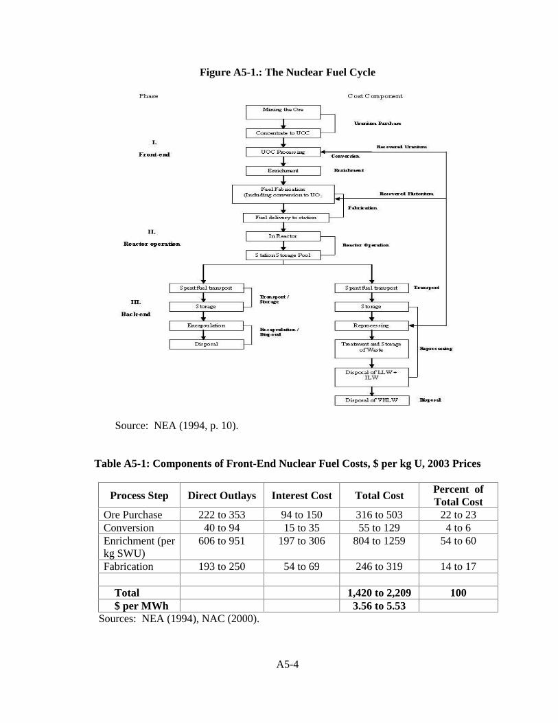
A5-4

Figure A5-1.: The Nuclear Fuel Cycle

Source: NEA (1994, p. 10).

Table A5-1: Components of Front-End Nuclear Fuel Costs, $ per kg U, 2003 Prices

Process Step Direct Outlays Interest Cost Total Cost Percent ofTotal Cost

Ore Purchase 222 to 353 94 to 150 316 to 503 22 to 23Conversion 40 to 94 15 to 35 55 to 129 4 to 6Enrichment (perkg SWU)

606 to 951 197 to 306 804 to 1259 54 to 60

Fabrication 193 to 250 54 to 69 246 to 319 14 to 17

Total 1,420 to 2,209 100 $ per MWh 3.56 to 5.53

Sources: NEA (1994), NAC (2000).

A5-5

A5.3. Reprocessing Technologies, Leading to Recycling and Actinide Burning

The United States has thus far decided to forego the reprocessing route to employ aonce-through system (in which the nuclear fuel is used and then disposed). Chapter 7contains a summary of disposal policies in different countries. The 1977 decision not toreprocess was based in large part on concerns over nuclear proliferation because of theseparation of pure plutonium by PUREX reprocessing. This section describes the processingtechnology system that raised U.S. concerns over proliferation potential and recenttechnological advances that are reducing the scope for diversion of civilian nuclear materialto weapons.

Over the last 40 to 50 years, reprocessing has been used in some countries to recoverunused uranium and plutonium from spent fuel. Reprocessing involves dissolving the wastefuel to allow plutonium and uranium to be separated from the other wastes. Spent fueltypically contains a little over 1 percent by weight of plutonium, about 95 percent uraniumand about 4 percent waste products. The separated uranium can be enriched again for use asfuel, while the plutonium is made into mixed oxide (MOX) fuels (Bunn et al. 2003, pp. 2-3).

Reprocessing traditionally has been conducted through the PUREX process. PUREXis an aqueous process that involves shearing and dissolving spent fuel in nitric acid forsubsequent solvent extraction of plutonium and uranium from residual minor actinides andfission products. The spent fuel is unloaded from containers into an interim storage facilityand then remotely transferred to the preparation cell for cutting off, shearing and dissolutionin a shearing machine. After that, the extracted solution is transferred for clarification (toremove the suspended particles) and purification from fission products. Uranium andplutonium are chemically separated and eventually consumed in future reactors. Theremaining liquid is high-level waste, which is stored in cooled tanks prior to vitrification and,later disposed in a deep geological repository.

Since reprocessing followed by multiple recycles and actinide burning reduces thevolume and long term toxicity of nuclear wastes, it could be used in conjunction with otherstorage options to mitigate or defer capacity constraints. These possibilities will beconsidered in the analysis of the economic costs of disposal.

Reprocessing and recycle of the uranium and plutonium, and actinide burning infuture fast reactors provides another way to reduce the volume and toxicity of radioactivewaste for disposal.

In 1999, a new process, UREX, was proposed by DOE; the UREX process wasdeveloped as a more proliferation-resistant variation of PUREX; it is devised so that onlyuranium is separated as a pure product from the transuranics, (comprised of plutonium plusminor actinides) plus fission products. By preventing the separation of plutonium from theother radioactive species, it degrades the usability of plutonium for weapons applications.Then, the commixed transuranic product can be further processed to reduce the overallamount of high-level waste (UIC 2004).

A5-6

Pyroprocessing is a non-aqueous reprocessing technology, developed in the 1980’sand 1990’s for recycle of fast-breeder reactor fuel. Pyroprocessing separates actinides (i.e.,uranium plus transuranics) from fission products present in spent fuel. The mixture ofactinides produced results in an unusable form for weapons applications and can be recycledin fast reactors for further energy extraction. One of pyroprocessing’s main advantages iscompactness such that it can be conducted on-site, which eliminates the various costs andother risks of transportation. PYRO-A is a variant of pyroprocessing designed to follow afterthe UREX process, in which the mixture of transuranics (i.e., plutonium plus minoractinides) from UREX are further separated from the fission products. The fission productsare then converted into a ceramic composite for simpler disposal (UIC 2004).

A5.4. DOE Advanced Fuel Cycle R&D

Near-term goals for DOE’s advanced fuel cycle research are to further developproliferation-resistant processes that reduce total spent fuel volume, separate long-livedhighly toxic elements, and reclaim spent fuel’s valuable energy (DOE 2003a). These includedevelopment of spent fuel treatment processes such as uranium extraction (UREX andUREX +) technology and pyroprocessing, as well as development of fuels that allow thetransmutation of plutonium into elements that cannot be used for nuclear weapons.

Longer-term goals are to explore methods that would reduce the long-termradiotoxicity and heat load of high-level waste sent to repositories. Research into thedevelopment of next-generation nuclear fuel cycles seeks to simultaneously increase theenergy production derived from nuclear fuels and to ease the radioactive waste disposalprocesses. Possibilities include the fast neutron spectrum reactors or accelerators tofacilitate transmutation of the actinides.

A5.5. Costs of Direct Disposal and Projections of Costs for Reprocessing

The back-end fuel cycle cost consists of temporary storage at the site of the nuclearpower generation, followed by permanent disposition at a central facility such as YuccaMountain. The first sub-section below estimates these costs, on a per kWh basis, if the spentfuel is not reprocessed. The second sub-section estimates the costs if spent fuel isreprocessed. The final sub-section compares the full back-end costs with and withoutreprocessing.

A5.5.1. Direct Disposal

Nuclear plants were designed to temporarily store spent nuclear fuel (SNF) before itis transferred to a final repository. On-site storage uses water pools (also known as wetstorage), which keeps the fuel cool as it undergoes radioactive decay. Recently, dry caskstorage has been used to store SNF that has been water-cooled for one year in sealed steel

A5-7

casks to increase the available on-site storage capacity. Wet and dry on-site storage,however, are considered temporary solutions, as they are intended to allow fresh SNF to coolbefore its final disposal (Bunn et al. 2001, p. 10).

Since the early 1980s, Yucca Mountain, Nevada, has been the site proposed by DOEfor the construction of a centralized high-level radioactive waste storage facility. The planscall for a permanent underground storage complex intended to house all of the high-levelradioactive waste that currently exists in the United States and that will be produced in thiscountry through the year 2041. The Yucca Mountain project is projected to proceed instages: development (1983 to 2003), licensing (2003 to 2006), construction (2006 to 2010),emplacement (2010 to 2041), monitoring (2041 to 2110), and closure (2110 to 2119) (DOE2002).

The Yucca Mountain project has been funded in two main ways. Congress has madeappropriations to cover the disposal of defense-related nuclear wastes, while a tax of one 1mill (one-tenth of a cent) per kWh since 1983 has been levied on power produced at nuclearpower plants in order to fund the disposal of commercially produced wastes. As of this date,the fund totals almost $18 billion. The money from this fund, along with the proceeds fromits investment income over the coming decades, has been projected to be sufficient to pay forthe Yucca Mountain project.

While Yucca Mountain’s currently legislated capacity is 70,000 metric tons, DOE’sEnvironmental Impact Statement suggests that the site could safely accommodate more than120,000 metric tons (DOE 2002). Other sources suggest 150,000 to 200,000 metric tons maybe possible (Peterson 2003, p. 28; NEI 2003).

With regard to estimation of disposal costs, for the temporary on-site storage phasetotal capital cost to establish new dry storage facilities at a reactor site is estimated to rangefrom $8 to $12 million regardless of the amount of waste to be generated (Bunn et al. 2001,p. 13). Costs to purchase and load dry casks range from $60 to $80 per kilogram of heavywaste (kgHM). Operating costs are modest since there is little to be done after loading,except security and safety monitoring, maintaining its NRC license. For a reactor thatgenerates 1,000 metric tons of heavy metal waste over a 40-year lifetime, the total cost for5 years of dry cask storage would be approximately $120 million. Assuming the plantgenerates 0.006 lbs. of spent nuclear waste per MWh (DOE 2003b), the cost to a 1,000 MWreactor would be 0.09 mills per kWh, or $0.09 per MWh.

For permanent disposal, the estimated total cost for disposal at Yucca Mountain isapproximately $56 billion. This includes an estimated $49.3 billion in future costs and$6.7 billion in past costs (DOE 2001a, p. 1-1). This cost estimate covers every stage of theYucca project, from development to permanent closure. DOE’s (2001b) recent investigationof the current fee system determined that the charge of 1 mill per kWh is sufficient to coverthe costs of storing all high-level wastes generated through 2041. Calculations belowcorroborate this assessment.

A5-8

The commercial cost per kWh excludes disposal costs for defense-related wastes,which are anticipated to comprise 10 percent of the total volume but will account for29 percent of the total cost (DOE 2001b, p. 4). For purposes of this analysis, the 29 percentportion of defense-related appropriations is excluded from the commercial cost calculation.The remaining 71 percent of the total cost amounts to $39.8 billion. Assuming an expandedcapacity of 120,000 metric tons, and debiting 10 percent for defense-related wastes, leaves108,000 metric tons of current and future commercial nuclear waste to pay for the$39.8 billion in total costs of Yucca Mountain. These figures are converted to a kWh costbasis as follows: $39.8 billion ÷ [(108,000 metric tons waste x 2,200 lbs per metric ton) ÷(0.006 lbs per MWh ÷ 1,000 kWh per MWh)] = 0.001. Thus, the cost of disposal at YuccaMountain storage is projected to be about 1 mill per kWh, or about $1 per MWh.

A5.5.2. Reprocessing, Recycling, and Actinide Burning

As the United States has not reprocessed nuclear fuel for many years, any estimate ofthe effect of reprocessing on back-end costs in this country remains especially tentative(Bunn et al. 2003). However, British Nuclear Fuels, Ltd. (BNFL) in the U.K. and COGEMAin France offer reprocessing services internationally, and their prices can be used as roughguideposts to potential U.S. reprocessing costs.

The U.S. scenario involves reprocessing and permanent storage at Yucca Mountain.The cost of reprocessing per kg of usable fuel includes $63 per kg for transportation of wastefuels, and $904 per kg for the reprocessing cost for a total of $967 per kg (NEA 1994, p.12,converting to 2003 prices). Capital costs are included in the $904 per kg reprocessing cost.A kg of UO2 reactor fuel yields approximately 399,000 kWh (NAC, 2000). Expressing thereprocessing cost on a per kWh basis, $967 per kg of fuel/399,000 kWh per kg fuel = 2.4mills per kWh, or $2.40 per MWh, for the reprocessing costs.

For comparison, independent estimates of the relative costs of reprocessing versus no-reprocessing are available. Based on uranium prices of about $50 per kg U3O8 and usingstatistical analysis to take standard deviations around mean values, NEA (1994, p. 14)estimates a spread of 0.95 to 1.11 mills per kWh (converted to 2003 prices) for the differencebetween treating and not treating spent fuel. Lobdell (2002, p.18) estimates 1.82 mills perkWh difference between reprocessing and not reprocessing for the United States. Bunn et al.(2003, executive summary), who annuitize the costs of new processing facilities into theircost estimate of reprocessing, report an increase in cost of 1.3 mills per kWh fromreprocessing, using a uranium price of $40 per kg and a reprocessing price of $1,000 perkgHM. An average of these cost estimates and that estimated here is about 1.65 mills perkWh, or $1.65 per MWh. The fabrication costs, associated with recycling plutonium anduranium, as well as the added reactor cost of consuming this material would need to beincluded in the overall calculation.

Under the disposal alternative considered in this sub-section, the total amount ofheavy metal waste would be reduced to approximately 887 kg per year or 35.5 metric tonsover a 1,000 MW reactor’s lifetime (MIT 2003, p. 30). Using the costs above, the total life

A5-9

cycle cost of 5 years’ dry storage would be about $43 million dollars or $1,210 per kgHM.Assuming a plant using reprocessing generates 0.00011 kg of heavy metal waste per MWh,the cost of on-site storage for 5 years would be 0.05 mills per kWh. This estimate could beaffected if the actinides are not consumed prior to disposal, since the costs for disposal arehighly dependent upon the relative toxicity of the fuel.

Peterson (2003, p. 28) estimates the technical capacity of Yucca Mountain for fissionproducts from a closed fuel cycle to be 200,000 MT, which is larger than the 120,000 MTassumed for the direct disposal because the fission products separated in the reprocessing canbe packed more closely together. Reserving 10 percent of the total capacity for defense-related wastes, the total capacity available for commercial wastes is 180,000 MT. Assumingthat the total cost of Yucca Mountain continues to be $39.8 billion and 0.00011 kg of fissionproducts per MWh is produced (MIT 2003, p. 30), the incremental cost of storage at YuccaMountain would be 0.24 mills per kWh, or $0.24 per MWh. This estimate, additionally,could be affected if the actinides are not consumed prior to disposal.

A5.5.3. Summary

Table A5-2 summarizes the cost components of direct disposal, or the back-end costsof the fuel cycle currently used in the United States. The cost estimates calculated here aretentative and rely on approximations which could be refined. Nevertheless, they point tomagnitudes which, even if raised by a factor of two or three, would still be small.

Table A5-2: Disposal Costs, $ per MWh, 2003 Prices

A5.6. Total Fuel Cycle Costs

Table A5-3 adds the front-end and back-end costs of nuclear fuel for direct disposal.This includes temporary storage on-site of $0.09 per MWh and the $1 per MWh fee fordisposal at Yucca Mountain, yielding a total fuel cycle cost of $5.44 per MWh.

Fuel Cycle Component CostTemporary on-site storage 0.09Permanent storage at Yucca Mountain 1.00TOTAL 1.09

A5-10

Table A5-3: Fuel Cycle Cost Components under Direct Disposal,$ per MWh, 2003 Prices

Fuel Cycle Component CostFront-end cost 4.35Temporary on-site storage 0.09Disposal at Yucca Mountain 1.00TOTAL 5.44

Three sensitivities of the estimates in Table A5-3 may be noted. First, the range offront-end costs associated with disposing of the fuel directly, from Table A5-1, is $3.56 to$5.53 per MWh, which yields a range in total fuel cycle costs of $4.65 to $6.62 per MWharound the $5.44 mid-range estimate in Table A5-3 for the benchmark situation of noreprocessing. Second, a doubling of the price of uranium ore would increase the total fuelcycle cost in Table A5-2 by $0.61 per MWh. Third, if long-term storage on site wererequired due to delay in opening Yucca Mountain, the cost of on-site storage would risemodestly, by $0.43 per MWh. None of these sensitivities materially affects nuclear power’sLCOE.

A5.7. Conclusion

Fuel cycle costs are not a major factor in the economic competitiveness of nuclearpower. The larger waste disposal questions, involving advanced fuel cycles, concern broadpolicy issues related to proliferation issues considered in Appendix A7.

A5-11

References

Bunn, Mathew, John P. Holdren, Allison Macfarlane, Susan E. Pickett, Atsuyuki Suzuki,Tatsujiro Suzuki, and Jennifer Weeks. (2001) “Interim Storage of Spent Nuclear Fuel.”Cambridge, Mass.: Joint report, Harvard University and Tokyo University.

Bunn, Matthew and Steve Fedder, John P. Holdren, Bob van der Zwaan. (2003) “TheEconomics of Reprocessing vs. Direct Disposal of Spent Nuclear Fuel.” Cambridge, Mass.:Harvard University, Project on Managing the Atom.

Lobdell, Simon. (2002) “The Yucca Mountain Repository and the Future of Reprocessing.”Mimeo. Washington, D.C.: Washington Internship for Students of Engineering.

Macfarlane, Allison. (2001) “Interim Storage of Spent Fuel in the United States,” AnnualReview of Energy and the Environment 26: 201-35.

Massachusetts Institute of Technology (MIT). (2003) The Future of Nuclear Power: AnInterdisciplinary MIT Study. Cambridge, Mass.: Massachusetts Institute of Technology,July.

Nuclear Assurance Corporation (NAC). (2000) Nuclear Fuel Management Seminar. PowerPoint slides. November.

Nuclear Energy Institute (NEI). (2003) “Common Objections to the Yucca MountainProject, and What the Science Really Says.” Retrieved August 15, 2003 from the WorldWide Web: http://www.nei.org/index.asp?catnum=2&catid=197.

Nuclear Energy Agency (NEA). (1994) The Economics of the Nuclear Fuel Cycle. Paris:OECD.

Peterson, Per F. (2003) “Will the United States Need a Second Geologic Repository?” TheBridge 33, No. 3: 26-32.

Uranium Information Centre (UIC). (2004) “Waste Management in the Nuclear FuelCycle.” Nuclear Issues Briefing Paper 9. Melbourne, January.

U.S. Department of Energy (DOE). (2001a) “Analysis of the Total System Life Cycle Costof the Civilian Radioactive Waste Management Program.” Washington, D.C., May 2001.

U.S. Department of Energy (DOE). (2001b) “Nuclear Waste Fund Fee Adequacy.”Washington, D.C.

U.S. Department of Energy (DOE). (2002) “Yucca Mountain: Commonly Raised Topics.”Pamphlet. Washington, D.C.

A5-12

U.S. Department of Energy (DOE). (2003a) Report to Congress on Advanced Fuel CycleInitiative: The Future Path for Advanced Spent Fuel Treatment and TransmutationResearch. Washington, D.C.: Office of Nuclear Energy, Science, and Technology, January.

U.S. Department of Energy (DOE). (2003b) “Nuclear Issues.” Retrieved from the WorldWide Web: http://www.eia.doe.gov/cneaf/nuclear/page/nuclearenvissues.html.

World Nuclear Association (WNA). (2003) “Economics of Nuclear Power.” October 2003.Retrieved from the World Wide Web: http://www.world-nuclear.org/info/inf02.htm.

A6-1

Appendix A6. NUCLEAR REGULATION

Summary

The U.S. Nuclear Regulatory Commission (NRC) was created to conduct all licensingand regulatory functions for the nuclear power industry. It is involved in the regulation ofactivities from mining uranium to plant decommissioning. Historically, the construction andoperation permitting process has been at the center of many delays and cost increases for newnuclear power plants.

An amendment to the Code of Federal Regulations (10 CFR Part 52) provides forcombined construction and operation permitting and is aimed at streamlining the permittingprocess. The combined Part 52 license is designed to allow investors the opportunity toresolve many uncertainty issues before committing large amounts of money to an investmentin a nuclear facility.

Reducing construction delays and lowering the risk premium to investors necessary tocompensate for the possibility of delays or cancellations due to regulatory activities couldlower the cost of power from a nuclear plant significantly. Table A6-2, derived from thefinancial model of Chapter 5, compares levelized cost of power (LCOE) for nuclear plantsunder different regulatory regimes. The first regime, reflecting the older procedure, assumes7-year construction time, 12 percent interest rate on debt, 15 percent required return onequity, and a reduction in construction costs of 3 percent for doubling the number of plants.The second regime, reflecting the new regulatory procedures, assumes a 5-year constructiontime, 7 percent interest rate on debt, 12 percent required return on equity, and 5 percentreduction in construction costs for double the number of plants. The electricity costreduction for lower cost plants is 31 percent and 53 percent for higher cost plants.

A6-2

Outline

A6.1. Introduction

A6.2. Current Regulatory Framework

A6.2.1. Mining RegulationsA6.2.2. Regulations for Importing and Exporting Nuclear Fuels and

EquipmentA6.2.3. Nuclear Facilities: Construction and Operation LicensesA6.2.4. Inspections and Reporting RequirementsA6.2.5. Regulating the Protection of Workers from RadiationA6.2.6. Emergency ResponseA6.2.7. Regulation of Radioactive WastesA6.2.8. Operating License RenewalA6.2.9. Decommissioning

A6.3. Major Regulatory Costs

A6.3.1. Costs of DelayA6.3.2. Costs on UncertaintyA6.3.3. Potential Benefits of Improved Regulation

A6.4. Conclusion

References

A6-3

A6.1. Introduction

This appendix examines the impacts of regulation on the future construction andoperation costs of nuclear power facilities. Section A6.2 reviews the current regulatoryframework. Section A6.3 presents estimates of costs of delay and uncertainty that may bereduced by streamlined regulation. Section A6.4 concludes that benefits of reducingconstruction delays and investor uncertainties are substantial.

A6.2. Current Regulatory Framework

Regulation of nuclear energy in the United States originates with the Atomic EnergyAct (AEA) of 1954 (42 USC 2011 et seq.) and is enumerated in the relevant sections of theCode of Federal Regulations (CFR). The federal government has assumed most regulatoryresponsibilities in this area; in fact, courts have struck down many state efforts to regulatenuclear energy more independently (Hillegas 1983). While states can still regulate thoseareas the federal government has chosen not to address, federal preemption has ensured theregulatory supremacy of the federal government in nuclear energy. The U.S. NuclearRegulatory Commission (NRC) was created to conduct all licensing and regulatory functions(Schoenbaum 1988).

A6.2.1. Mining Regulations

Although the AEA does not set forth detailed provisions regarding the mining ofuranium or thorium, NRC is responsible for issuing licenses for the extraction of thesematerials. In recent years, several U.S. facilities have been licensed to recover uranium(OECD 1999). DOE can also issue permits for uranium exploration on federal lands.

A6.2.2. Regulations for Importing and Exporting Nuclear Fuels and Equipment

In 1995, NRC issued rules making regulations on the import or export of nuclearfuels and equipment conform to the International Atomic Energy Agency’s (IAEA)principles of transboundary movement. The new standards, much like the old regulations,focus on issues of nuclear proliferation and require licenses to export or import nuclearwastes and mixed wastes. Separate categories and requirements exist for materials thatbecome incidentally radioactive. NRC consults with other federal agencies regarding exportsof radioactive materials and must receive explicit approval prior to transit from all affectedcountries.

A6.2.3. Nuclear Facilities: Construction and Operation Licenses

All nuclear power plants in the United States are licensed by NRC pursuant to theprovisions of the AEA. NRC’s Office of Nuclear Material Safety and Safeguards licensesfuel cycle facilities, and the Office of Nuclear Reactor Regulation issues reactor licenses(42 USC 5801-5844).

A6-4

For many years, NRC’s licensing process occurred in two steps, with the issuance ofa construction permit and then (two or three years before scheduled completion) an operatingpermit (10 CFR Part 50). These steps were consolidated and made part of the AEA in 1992,so that the entire licensing process could occur in one step (10 CFR Part 52). The one-steplicensing procedure was designed to allow an early resolution (or an earlier failure to reachresolution) of safety and operation issues. In particular, Part 52 requires early resolution ofsite suitability issues, emergency preparedness, and consideration of environmentallysuperior sites. For a summary of licensing procedures see Table A6-1 below.

The construction permit section must address (1) environmental and plant safety and(2) anti-trust issues. If NRC finds the application to be complete, a notice is published in theFederal Register and the application is distributed to all interested state and federal agencies.At this point, NRC’s review of the application includes a focus on several key areas: safety,environmental protection, and anti-trust.

A safety review for the proposed design is conducted pursuant to the StandardReview Plan, a guide containing detailed design information about every reactor system andcomponent. The Advisory Committee on Reactor Safeguards, an independently andstatutorily created body, also reviews the application for design and safety, and then issues anopinion to NRC regarding the sufficiency of the application.

An Environmental Impact Statement (EIS) is also prepared by NRC (pursuant to theNational Environmental Policy Act, NEPA), evaluating any environmental impacts of theproject. The draft EIS is published in the Federal Register for comment. NRC thenpublishes its final EIS, which addresses all comments received.

NRC also begins the anti-trust review and forwards this initial report to theDepartment of Justice (DOJ) for comment. When the Attorney General’s analysis and adviceis received, NRC publishes its final determination on the anti-trust issues.

The operation permit is intended to ensure that the plant has been constructed inaccordance with the approved construction design, and that the plant can operate safely.Under the old licensing system, this process began a few years prior to the completion ofconstruction, whereas Part 52 requires the applicant to submit the procedures it willundertake and acceptance criteria it will use to ensure that after construction the plant hasbeen built according to plan and can operate safely. Although these procedures andconditions are specified in advance, NRC must find that all of these criteria have been met.

After public hearings, NRC publishes a decision about the license application, whichmay be appealed directly to the Commission. After this first appeal, interested parties canappeal to the local U.S. Court of Appeals for further review.

A6-5

Table A6-1: Comparison of One-Step and Two-Step Licensing

Old Two-StepLicense Procedure

Construction Permit· Preliminary Safety Analyses· Environmental Review· Financial and Anti-Trust Statement· Public comment on each section

Operating License· Submission of Final Design· Final Environmental and Safety Analysis· Further public comment on each section

New One-StepLicense Procedure

Pre-Application Activities· Early Site Permit (includes environmental review)· Standard Reactor Design Certification· Public comment

Combined License· License Authorizes Construction and Operation· Includes same information as two-step procedure· Can reference early application activities· Public comment within 180 days of reactor start-up

A6.2.4. Inspections and Reporting Requirements

The operating license contains detailed provisions regarding periodic inspections(NEA 1999). NRC conducts regular safety inspections in conjunction with full-time reactorsite inspectors. The results of these inspections are published. Moreover, nuclear powerplants are periodically reviewed for other operational characteristics (called the SystematicAssessment of License Performance, or SALP). Throughout its operational life, the reactorfacility is also required to report specific types of information to NRC on a regular basis.

A6.2.5. Regulating the Protection of Workers from Radiation

Regulations applicable to worker safety at nuclear facilities attempt to (1) informworkers about the health problems from radiological exposure, (2) educate workers aboutmethods to reduce exposure, and (3) encourage workers to report problems to NRC (NEA1999). Some of the specific regulations include setting an annual limit for radiation doses,monitoring personnel for exposure, providing radiation protection equipment and the trainingto use it, informing workers about exposure hazards, and providing training regardingapplicable warning labels, instructions, and signs. In addition, nuclear plants are still subjectto all the requirements of the Occupational Safety and Health Act (OSHA).

A6-6

A6.2.6. Emergency Response

The Three Mile Island accident in 1979 resulted in no off-site radiological exposures,but it led to a more formalized system of emergency preparedness. NRC created standardsfor state and local emergency planning and required that these plans be made in conjunctionwith the Federal Emergency Management Agency (FEMA) (Goxem 1988). Thiscontingency planning includes emergency notification systems like sirens and broadcastwarnings, as well as periodic emergency drills.

A6.2.7. Regulation of Radioactive Wastes

NRC, DOE and EPA work together to regulate the management and disposal ofradioactive wastes in the United States. The regulatory framework, economic costs, andother issues related to this subject are discussed at length in Chapter 5.

A6.2.8. Operating License Renewal

Pursuant to the AEA, an operating license can be renewed (10 CFR Part 54).Currently, NRC regulations allow as many as 20 additional years of operation throughrenewal.

A6.2.9. Decommissioning

NRC’s responsibilities for health and safety carry over into the decommissioning ofnuclear power plants. Decommissioning is defined as taking a nuclear reactor safely off-lineand then reducing radioactivity to a level that permits unrestricted use of the site property.

A6.3. Major Regulatory Costs

Many of the regulatory requirements outlined above are similar to the types ofregulatory costs that many U.S. businesses face. Licensing and reporting requirements arecommon in many industrial sectors. These costs, although significant, are not unexpectedand are ordinary business expenses. Over the past decades, NRC, coordinating with thenuclear power vendors and utilities, has worked to create a less burdensome regulatorystructure while still protecting the public welfare (NRC 1978). Several major reports havehighlighted some areas for reform and improvement: (1) renegotiation of safety, security, andemergency programs that currently exceed NRC requirements; and (2) greater regulatoryflexibility about operation or construction matters that are economically advantageous andcause no reduction in safety (NEA 1998, NEA 1998, NRC 1978).

One baseline estimate for the cost of the regulatory process (essentially the feestructure for licensing and reporting without additional problems or delays) is approximately1 mill per kWh (The Nuclear Tourist 2003), or only $1 per MWh. The major

A6-7

regulatory costs have been due to unanticipated delays and uncertainty that can contribute tothe riskiness of investing in nuclear facilities

A6.3.1. Costs of Delay

Capital costs contribute 60 to 64 percent of the LCOE of nuclear power (see Table3-5). Interest costs over a 7-year construction period can be nearly 30 percent higher thanthey would be for the same overnight cost over a 5-year construction period (Table 3-6). Theresulting LCOE can be about $5 to $6 per MWh, or roughly 13 to 15 percent, higher as aconsequence. Expressed as a saving that could be obtained by reducing a construction periodfrom 7 years to 5, this amounts to a 12 to 13 percent saving.

Similarly, a two-year halt in the middle of construction could increase the LCOE of anuclear power plant by over $7 per MWh, and a two-year delay between the completion ofconstruction and bringing a nuclear plant on-line can add nearly $15 per MWh to its LCOE(Table 5-7). This is a possible additional cost that could be avoided, beyond the basic no-policy LCOE.

A6.3.2. Costs of Uncertainty

The risk that a plant, once begun, will not be completed or if completed will not beallowed to operate, makes investors skittish. Either they will require a higher risk premium,which will lead to a higher cost per megawatt hour of the power that eventually does getproduced from the plant, or they will decline to invest at all. Calculations in Chapter 9indicate that reducing the required risk premium on investment in a nuclear plant to levelscomparable to those for coal- and gas-fired plants would reduce the LCOE of the nuclearplant by $9 to $14 per MWh. This amounts to a reduction of roughly 26 to 32 percent foreighth plants, depending on the initial capital cost and the ability of learning by doing toreduce overnight costs (Tables 9-8 to 9-10). This combines the effect of the shortenedconstruction period, noted in the previous sub-section, at a given interest rate, and lowerinterest rates over the shorter construction period, resulting in a total reduction in LCOE of$14 to $21 per MWh.

A6.3.3. Potential Benefits of Improved Regulation

This section pulls together the construction-time and risk-reduction benefits thatimproved regulation could confer and takes into further consideration the expectation that asmoother regulatory procedure could enhance learning by doing. Table A6-2 compares theLCOE of an eighth plant under the previous regulatory regime with that of an eighth plantunder an improved regime. This comparison assumes that the former circumstances allow a3 percent learning rate—that is a 3 percent reduction in overnight costs with each plantdoubling—and that the improved circumstances permit a 5 percent learning rate. The firstrow of the table reports the LCOEs of the eighth plant of each design built in 7 years, atinterest rates of 12 percent on debt and 15 percent on equity, and with a 3 percent learningrate on overnight cost reductions. The $1,200 or $1,500 design would have an LCOE of

A6-8

$49 per MWh. The difference between these two beginning overnight costs is that FOAKEcosts have not been paid on the $1,500 plant; once those costs are paid, the learning effectsoperate on the same overnight costs across the two designs. The LCOE of the $1,800 designwould be $58 per MWh. These LCOEs are the result of status-quo regulation.

The second row reports the LCOEs for those plants, built in 5 years, at interest ratesof 7 and 13 percent on debt and equity, and with a 5 percent cost reduction for learning. TheLCOE for the $1,200 or $1,500 design is $34 per MWh, and that for the $1,800 design is$43. These LCOEs are the result of the improvements in the regulatory procedures.

The third row reports the percent reduction in LCOE that would derive from theimprovements in regulation between rows one and two. The improved regulation wouldyield a 31 percent reduction in eighth plant LCOE for the $1,200 and $1,500 designs and a53 percent reduction for the $1,800 design. The difference in percent LCOE reduction is dueto the different capital costs: the larger capital-cost plant benefits proportionally morebecause the levelized capital component of its LCOE is larger.

Table A6-2: LCOEs for Eighth Nuclear Plants, with No Policy Assistance Other thanImproved Regulation, $ per MWh, 2003 Prices

Beginning Overnight Cost, $ Per kW1,200 or 1,500 1,800

7-year construction timeInterest rates: 12 percent on debt, 15 percent on equity

Learning effect: 3 percent reduction in cost for doubling plants built49 58

5-year construction timeInterest rates: 7 percent on debt, 12 percent on equity

Learning effect: 5 percent reduction in cost for doubling plants built34 38

Percent reduction in LCOE due to improved regulation31 53

A6.4. Conclusion

In sum, the benefits of reducing construction delays and investor uncertainties aresubstantial. Shortening the construction period and reducing the risk premium can have acombined effect of reducing a nuclear plant’s LCOE by 30 percent.

A6-9

References

Center for Strategic and International Studies. (1999) The Regulatory Process for NuclearPower Reactors. Washington, D.C.: CSIS Press.

Hillegas, Joe. (1983) “Pacific Gas and Electric Co. v. State Energy Resources Conservationand Development Commission: Preemption of State Regulation of Nuclear Power,” Journalof Energy Law and Policy 5: 135-46.

Goldsmith, Richard. (1991) “Regulatory Reform and the Revival of Nuclear Power,” HofstraLaw Review 20: 159-208.

Goxem, Karen. (1988) “Emergency Offsite Planning for Nuclear Power Plants; FederalVersus State and Local Control,” American University Law Review 37: 417-51.

Moeller, James. (1992) “State Regulation of Nuclear Power and National Energy Policy,”Journal of Energy, Natural Resources, and Environmental Law 12: 1-61.

Nuclear Energy Agency (NEA). (1998) Future Nuclear Regulatory Challenges. Paris:OECD.

Nuclear Energy Agency (NEA). (1999) Regulatory and Institutional Framework for NuclearActivities. Paris: OECD.

The Nuclear Tourist. Retrieved December 20, 2003 from the World Wide Web:http://www.nucleartourist.com/.

Reitze, Arnold. (1987) “The Price-Anderson Act - Limited Liability for the NuclearIndustry,” Environmental Law Reporter 17: 10185-114.

Schoenbaum, Thomas. (1988) The Regulation of Nuclear Power in Three Countries: TheUnited States, France, and Japan. Athens, Ga: The Dean Rusk Center.

U.S. Nuclear Regulatory Commission (NRC). (1978) Preliminary Statement on GeneralPolicy for Rulemaking to Improve Nuclear Power Plant Licensing. Washington, D.C.

A6-10

A7-1

Appendix A7. NONPROLIFERATION GOALS

Summary

Countries that have chosen reprocessing include Belgium, China, France, Germany,India, Japan, Russia, Switzerland, and the U.K. These countries engage in reprocessing toseparate plutonium and uranium from fission products for further use as fuel for reactors.Countries that have chosen direct disposal without reprocessing include the United States,Canada, Finland, South Korea, Spain, and Sweden. A chief concern with reprocessing is thatthe plutonium could be diverted to develop nuclear weapons. Several industrial countrieshave, in the past, provided reprocessing as well as enrichment technology and services toothers, purportedly increasing the opportunities for theft or transfer of technology,equipment, or products.

International regulation of nuclear energy takes the form of a combination of treaties,international organizations and multilateral and bilateral agreements. The key componentsare the Treaty on the Non-Proliferation of Nuclear Weapons, the International AtomicEnergy Agency, whose safeguards system verifies compliance, informal international groupsand the Convention on Physical Security for Nuclear Materials, which sets internationalsecurity standards for storing, using and transporting nuclear material. Implementation of thePresident’s February 11, 2004, speech would provide added safeguards preventingreprocessing and enrichment technology spreading to rogue countries or terrorists.

Resolution of these issues involves broader policy considerations beyond the scope ofthe present study. The future economic viability of nuclear power, however, does not dependon their resolution. As Appendix A6 shows, the difference in the cost of nuclear wastehandling, as between once-through disposal and reprocessing, is too small to materially affectthe economic viability of nuclear power.

A7-2

Outline

A7.1. Introduction

A7.2. International Comparison of Nuclear Fuel Disposal Policies

A7.3. The Nonproliferation Regulatory Framework

A7.3.1. The Treaty on the Non-Proliferation of Nuclear WeaponsA7.3.2. Role of the International Atomic Energy Agency (IAEA)A7.3.3. Other Regulatory Arrangements

A7.4. Current Administration Policy Regarding Nonproliferation Applicable to theNuclear Fuel Cycle

A7.5. Conclusion

References

A7-3

A7.1. Introduction

This appendix reviews practices in different countries (Section A7.2), andsummarizes international arrangements aimed at preventing proliferation (Section A7.3).Section A7.4 provides information on the current Administration policy regarding thespreading of enrichment and reprocessing technology outside a set of countries considered tobe reliable fuel suppliers who in compliance with international nonproliferationrequirements. The concluding section assesses the implications of proliferationconsiderations for the present study.

A7.2 International Comparison of Nuclear Fuel Disposal Policies

Technological considerations in direct disposal and reprocessing were discussed inAppendix A5. Attention was given to the traditional PUREX method of reprocessing and thenewer UREX method, along with further DOE developmental efforts. Countries havereacted differently to the technological alternatives. Table A7-1 provides a comparison offuel cycle and nuclear waste disposal policies.

Reprocessing separates plutonium and uranium from fission products and recoversthem for use as new fuel for reactors while reducing the volume of high-level waste and theradioactivity life of low-level waste. The recovered plutonium is stored in facilitiescontrolled by the International Atomic Energy Agency (IAEA) or is combined with uraniumand manufactured into mixed oxide (MOX) fuel used to feed certain type of nuclear reactors.The remaining radioactive liquid fission products are mixed with other materials, vitrified,and placed in metal canisters for storage. Among the countries conducting reprocessing thatwere mentioned above, France, the U.K., and Russia have large-scale reprocessing facilitiesand provide reprocessing services commercially to a number of other countries. Belgium andItaly have reprocessing facilities for research, and Japan is building a commercialreprocessing facility. Also, enrichment technology is located in several Western countries,Russia, and the Far East.

In the United States, reexamination of the U.S. choice of once-through policy isoccurring, in order to consider proliferation resistance characteristics of the newer UREX andPYRO methods of reprocessing and further DOE development of disposal technologiesdiscussed in Appendix A5. These techniques may be able to meet nonproliferation goalssince they do not require plutonium to be separated from higher actinides or transported sincethey are recycled together in the reactor. As a consequence, proliferation risks are lowered,mainly through a substantial reduction in the risk of theft or misuse of plutonium.

A7-4

Table A7-1: International Comparison of Nuclear Waste Disposal Policies

Country Fuel Cycle Policy Facilities and Progress toward Final RepositoriesBelgium Reprocessing Central waste storage and underground laboratory

established. Construction of repository to begin about2035.

Canada Direct Disposal Underground repository laboratory established.Repository planned for use in 2025.

China Reprocessing Central spent fuel storage in Lan ZhouFinland Direct Disposal Spent fuel storage in operation. Site selection studies

underway for deep repository for commissioning in2020.

France Reprocessing Two facilities for storage of short-lived wastes. Siteselection studies underway for deep repository forcommissioning in 2020.

Germany Reprocessing (underreview)

Low-level waste (LLW) sites in use since 1975. High-level waste (HLW) repository to be operational after2010.

India Reprocessing Research on deep geological disposal for HLW.Japan Reprocessing LLW repository in operation. HLW storage facility at

Rokkasho-mura; investigations begun for deepgeological repository.

Russia Reprocessing Sites for final disposal under investigation.South Korea Direct Disposal Central interim HLW storage planned for 2016. Central

LLW and intermediate level waste (ILW) repositoryplanned for post-2008. Investigating deep HLWrepository sites.

Spain Direct Disposal LLW and ILW waste repository in operation. Finalrepository site selection program for commissioning in2020.

Sweden Direct Disposal Central spent fuel storage facility in operation since1985. Final repository for LLW and ILW in operation.Underground research laboratory for HLW repository.Site selection for repository underway, to begin disposalin 2008.

Switzerland Reprocessing Central interim storage for all wastes underconstruction. Underground research laboratory for high-level waste repository, with deep repository to becompleted by 2020.

United Kingdom Reprocessing LLW repository in operation since 1959. HLW isvitrified and stored. Underground HLW repositoryplanned.

United States Direct Disposal Three LLW sites in operation. Decision in 2002 toproceed with geological repository at Yucca Mountain.

Source: UIC (2004, pp. 9-10).

A7-5

A7.3. The Nonproliferation Regulatory Framework

The nuclear nonproliferation regime consists of a combination of treaties,international organizations, and multilateral and bilateral agreements complemented byseveral unilateral actions intended to deter further spread of nuclear weapons. Keycomponents of the regime are the Treaty on the Non-Proliferation of Nuclear Weapons(NPT), the International Atomic Energy Agency (IAEA), whose safeguards system verifiesNPT compliance, informal international groups, and the Convention on Physical Security forNuclear Materials, which sets international security standards for storing, using andtransporting nuclear material. This section describes the extent of the NPT, the role of IAEAas well as its mission and safeguards system, and the responsibility of other organizationsand arrangements.

A7.3.1. The Treaty on the Non-Proliferation of Nuclear Weapons

The Nuclear Nonproliferation Treaty (NPT) was concluded in 1968, came into forcein 1970, and was indefinitely extended in 1995. Its main goals are to prevent the spread ofnuclear weapons, to make sure that peaceful nuclear technology is not diverted, to facilitateaccess to peaceful nuclear technology, and to promote disarmament. It provides the legal andinstitutional basis for nonproliferation internationally and depends for its success oncountries not violating their commitments. In particular, it establishes the framework for aninspection system based on an agreement between each participating state and IAEA.Currently, 187 nations are party to the NPT.

A7.3.2. Role of the International Atomic Energy Agency (IAEA)

IAEA was created in 1957 to help nations develop nuclear energy for peacefulpurposes. It has the role of establishing and administering nuclear safeguards arrangements,which are designed to deter diversion of nuclear material.

One of IAEA’s missions is to verify through its inspection system that states complywith their commitments under the NPT and other nonproliferation agreements, to use nuclearmaterial and facilities only for peaceful purposes.

Article II of the basic Statute of IAEA specifies the role of IAEA in terms ofpreventing nuclear proliferation: “the Agency shall seek to accelerate and enlarge thecontribution of atomic energy to peace, health and prosperity throughout the world. It shallensure, so far as it is able, that assistance provided by it or at its request or under itssupervision or control is not used in such way as to further any military purpose” (IAEA1997).

Part B of Article III indicates that “in carrying out its functions, the Agency shallconduct its activities in accordance with the purposes and principles of the United Nations topromote peace and international co-operation, and in conformity with policies of the United

A7-6

Nations furthering the establishment of safeguarded worldwide disarmament and inconformity with any international agreements entered into pursuant to such policies…”(IAEA 1997). It also mentions that the Agency shall “establish control over the use ofspecial fissionable materials received by the Agency, in order to ensure that these materialsare used only for peaceful purposes…” (IAEA 1997). Additionally, Article XI, Part F(4)indicates that assistance to members provided by the Agency for any project shall not be usedin such a way as to further any military purpose and that the project shall be subject to thesafeguards.

In its medium-term strategy statement IAEA recognizes the trend in the worldtowards a greater emphasis on the need for more effective verification of nonproliferationundertakings through strengthened safeguards covering both declared and undeclared nuclearmaterial and activities. In addition, according to the Agency, “there is a prospect of a globalban on the production of fissile material for explosive purposes, which could entail majorexpansion of the Agency’s verification activities” (IAEA 2001). Accordingly, one of thethree medium-term substantive objectives of IAEA is to ensure the peaceful use of nuclearmaterial. This implies providing greater assurance that countries are fulfilling theirnonproliferation commitments, assisting the international community in nuclear arms controland reduction efforts and improving the security of nuclear material.

A7.3.3. Other Regulatory Arrangements

While the IAEA was beginning to develop its regulatory system, several establishedregional organizations took the same path. Six western European nations establishedEURATOM as the nuclear branch of the European Economic Community, and afterwards,the Organization for European Economic Co-operation established the European NuclearEnergy Agency (ENEA). Both bodies set up their own administrative regulations, includingsafeguards systems. Later, formal relationships related to the safeguards were establishedbetween these agencies and the IAEA. For example, a formal agreement between individualcountries, EURATOM, and IAEA leads the implementation of safeguards in many countriesin Europe.

Two fundamental objectives of the EURATOM Treaty are to ensure theestablishment of the basic installations necessary for the development of nuclear energy inthe Community, and to ensure that all users in the Community receive a regular and equitablesupply of nuclear fuels. Additionally, other treaties of global scope with an objective ofdisarmament rather than nonproliferation are supporting the regime. As an illustration, thePartial Test Ban Treaty (PTBT), which prohibits open nuclear weapon tests, wasimplemented in 1963. Also, NPT participants reaffirmed their commitment to prohibit theproduction of any further fissile material for weapons in 1995, leading to the ComprehensiveTest Ban Treaty (CTBT).

A7-7

A7.4. Current Administration Policy Regarding Nonproliferation Applicable to theNuclear Fuel Cycle

In a recent speech at the National Defense University, President Bush said, “The 40nations of the Nuclear Suppliers Group should refuse to sell enrichment and reprocessingequipment and technologies to any state that does not already possess full-scale, functioningenrichment and reprocessing plants. This step will prevent new states from developing themeans to produce fissile material for nuclear bombs. Proliferators must not be allowed tocynically manipulate the NPT to acquire the material and infrastructure necessary formanufacturing illegal weapons” (Bush 2004).

A7.5 Conclusion

There is a lack of agreement about whether or not the availability of currentreprocessing and enrichment technology under current regulatory mechanisms are increasingnonproliferation risk. Pursuing proliferation-resistant fuel cycle technology will clearly allaythese concerns. Also, implementation of the President’s policy of capping the spread ofenrichment and reprocessing technology would provide added safeguards to preventreprocessing or enrichment technology spreading to rogue countries or terrorists.

Resolution of these issues involves broader policy considerations beyond the scope ofthe present study. The future economic viability of nuclear power, however, does not dependon their resolution. As Appendix A6 shows, however, the difference in the cost of nuclearwaste handling, as between once-through disposal and reprocessing, is too small to materiallyaffect the economic viability of nuclear power.

A7-8

References

Bush, George W. (2004) “Remarks by the President on Weapons of Mass DestructionProliferation.” National Defense University, Fort Lesley J. McNair, Washington, D.C.,February 12.

International Atomic Energy Agency (IAEA). “Mission Statement.” Retrieved from theWorld Wide Web: www.iaea.org.

International Atomic Energy Agency (IAEA). (2001) “Medium-Term Strategy 2001-2005.”Retrieved from the World Wide Web: www.iaea.org.

International Atomic Energy Agency (IAEA). (1997) “Statute: Last Amended 1989.”Retrieved from the World Wide Web: www.iaea.org.

International Atomic Energy Agency (IAEA). (1999) “Status and Trends in Spent FuelReprocessing.” Vienna: Proceedings of an Advisory Group Meeting, September 7-10.

Uranium Information Centre (UIC). (2004) “Waste Management in the Nuclear FuelCycle.” Nuclear Issues Briefing Paper 9. Melbourne, January.

U.S. Department of Energy (DOE). (2003). “Advanced Fuel Cycle Initiative (AFCI)Comparison Report, FY 2003.” Washington, D.C.: Office of Nuclear Energy, Science andTechnology, October.

World Nuclear Association (WNA). (2002b) “Mixed Oxide Fuel (MOX).” Retrieved fromthe World Wide Web: http://world-nuclear.org/info/inf29.htm.

A8-1

Appendix A8. HYDROGEN

Summary

Success in the current efforts to make the hydrogen car an economic reality wouldreduce U.S. dependence on foreign oil and could have potentially large environmentalbenefits. Intensive R&D efforts are underway to reduce fuel cell costs. Mass productioncosts need to be reduced on the order of one-half to two-thirds to achieve widespreadadoption.

Combining hydrogen with oxygen creates essentially no pollution since the by-product of this type of energy conversion is water. The environmental benefits of hydrogenwould however be tempered if fossil fuels with their attendant carbon emissions are used toproduce the hydrogen, simply replacing carbon emissions from oil with emissions from fossilpower generation or steam methane reforming. Nuclear energy may provide a pollution-freeinput for production of hydrogen. Hydrogen could be produced using electricity fromnuclear power in an electrolysis process, or it could be produced using thermo-chemicalprocesses with nuclear reactors as the energy source. A hydrogen economy accompanied bymore stringent efforts to control carbon emissions could greatly expand the demand fornuclear power.

A8-2

Outline

A8.1. Introduction

A8.2. Hydrogen-Fueled Vehicles

A8.2.1. Challenges to the Creation of a Hydrogen Vehicle FleetA8.2.2. Hydrogen Fuel CellsA8.2.3. Hydrogen Fuel Distribution InfrastructureA8.2.4. Viewpoints on the Prospects of the Hydrogen FCV

A8.3. Considerations for Large-Scale Hydrogen Production

A8.4. Hydrogen Production Techniques

A8.4.1. Steam Methane ReformingA8.4.2. ElectrolysisA8.4.3. Thermo-Chemical Cycles

A8.5. Conclusion

References

A8-3

A8.1. Introduction

If the hydrogen fuel cell vehicle makes a significant market penetration, the demandfor hydrogen will increase dramatically, and new sources for its production must be found.One promising possibility would use high-temperature nuclear reactors to provide the heatsource for steam methane reforming or thermal cracking. This appendix considers theprospects for a hydrogen economy to provide additional benefits from nuclear powergeneration. First, the hydrogen fuel cell vehicle (FCV) is considered: the near-term prospectsfor its market penetration and the demand for hydrogen that would derive from itswidespread adoption. Following the consideration of the FCV, the prospects for generationof hydrogen from nuclear power are examined.

A8.2. Hydrogen-Fueled Vehicles

The motivation to reduce air pollution and greenhouse gases caused by vehicleemissions, coupled with the need to reduce dependency on foreign oil, has speeded the raceto produce commercially viable vehicles that use gasoline-alternative fuel such as batteryhybrid vehicles and fuel cell vehicles. The hydrogen FCV has been given much attention inrecent years as an alternative to current gasoline-powered internal combustion engine (ICE)vehicles. The hydrogen FCV fits the category of zero-emission vehicle (ZEV) as itsbyproduct is water.

A8.2.1. Challenges to the Creation of a Hydrogen Vehicle Fleet

The successful introduction of hydrogen cars requires a hydrogen fuel cell capable ofpowering an automobile in a manner comparable to the internal combustion engine. On theinfrastructure side is the need for a distribution system to deliver the hydrogen fuel to thedriving consumer. The rest of this section will be primarily concerned with these two majorissues.

A8.2.2. Hydrogen Fuel Cells

A hydrogen fuel cell converts hydrogen and oxygen (or air) into water, producingelectricity and heat in the process. As hydrogen flows into the fuel cell on the anode side, aplatinum catalyst facilitates the separation of the hydrogen gas into electrons and protons(hydrogen ions). The hydrogen ions pass through a membrane (the center of the fuel cell)which acts as the electrolyte and, with the help of the platinum catalyst, combine withoxygen and electrons on the cathode side, producing water. The hydrogen electrons at thebeginning of the anode side which cannot pass through the membrane will flow from theanode to the cathode side through an internal circuit containing a motor or other electric load,which consumes the power generated by the cell.

A8-4

A8.2.2.1. Comparative Efficiency among the FCV, ICE and EV

A conventional internal combustion vehicle has an energy efficiency of 10 to 15percent. The hydrogen FCV is around 30 percent efficient. The hydrogen FCV is similar tothe battery-operated electric vehicle (EV) in that they both convert chemical energy intoelectricity and require minimal maintenance. The reactants in a battery are stored internallywhile the hydrogen fuel is stored externally in an FCV fuel tank. In this way, the hydrogenfuel cell is very much like a battery that can be recharged when drawing power from it,except that instead of recharging using electricity, a fuel cell uses hydrogen and oxygen. Abattery EV has only about 26 percent well-to-wheel efficiency, as energy is required forelectricity generation and a little energy is consumed in heat while operating the battery(Nice 2003). The hydrogen FCV has the highest efficiency among the three.

A8.2.2.2. The Components of the PEM Fuel Cell

The Polymer Electrolyte Membrane (PEM) fuel cell is one of the five types of fuelcell. It is the fuel cell that is under consideration by automobile manufacturers. Theelectrolyte in the PEM is a plastic or polymer membrane.

The electrodes separated by the membrane allow the electrochemical reaction to takeplace. The catalyst is a substance that participates in these reactions by increasing their rateof reaction but is not consumed in the reactions. A catalyst made of platinum works best forboth electrodes because it is sufficiently reactive in bonding the hydrogen and oxygenintermediates required to facilitate the electrode processes, and also is capable of effectivelyreleasing the intermediate to form the final product. The platinum catalyst is unique and is avery important part of the PEM fuel cell, but it is very expensive.

A8.2.2.3. Current Models of the FCV

The requirements for producing a FCV include the efficiency of the vehicle, ease ofrefueling, gas mileage, speed and performance, and design. Several automakers havesuccessfully designed and manufactured a hydrogen FCV which uses hydrogen as its fuel orhybrid FCV which runs on both hydrogen and battery. Honda, General Motors, and Toyotaare three of the leaders in the design of FCVs.

The Honda FCX has 80 horsepower and uses 201 ft-lb of torque. It has a maximumspeed of 93 mph, a 170-mile range, and accelerates from 0 to 60 mph in 10 seconds. It has45 percent efficiency and a fuel efficiency of 50 mpg. It weighs 3,713 lbs and is 166” inlength, 64.8” in height and 69.3” in width. The FCX electric motor produces an equivalentamount of torque to a Honda V6 engine, and its overall performance is comparable to aHonda Civic. Its 170-mile range is double the range of traditional battery-powered electricvehicles but only half of the range of gasoline cars. The Honda-designed Ultra usescapacitors to store energy generated by the fuel cell, and its regenerative braking provides

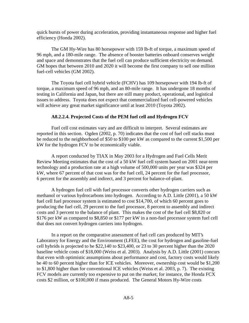
A8-5

quick bursts of power during acceleration, providing instantaneous response and higher fuelefficiency (Honda 2002).

The GM Hy-Wire has 80 horsepower with 159 lb-ft of torque, a maximum speed of96 mph, and a 180-mile range. The absence of booster batteries onboard conserves weightand space and demonstrates that the fuel cell can produce sufficient electricity on demand.GM hopes that between 2010 and 2020 it will become the first company to sell one millionfuel-cell vehicles (GM 2002).

The Toyota fuel cell hybrid vehicle (FCHV) has 109 horsepower with 194 lb-ft oftorque, a maximum speed of 96 mph, and an 80-mile range. It has undergone 18 months oftesting in California and Japan, but there are still many product, operational, and logisticalissues to address. Toyota does not expect that commercialized fuel cell-powered vehicleswill achieve any great market significance until at least 2010 (Toyota 2002).

A8.2.2.4. Projected Costs of the PEM fuel cell and Hydrogen FCV

Fuel cell cost estimates vary and are difficult to interpret. Several estimates arereported in this section. Ogden (2002, p. 70) indicates that the cost of fuel cell stacks mustbe reduced to the neighborhood of $50 to $100 per kW as compared to the current $1,500 perkW for the hydrogen FCV to be economically viable.

A report conducted by TIAX in May 2003 for a Hydrogen and Fuel Cells MeritReview Meeting estimates that the cost of a 50 kW fuel cell system based on 2001 near-termtechnology and a production rate at a high volume of 500,000 units per year was $324 perkW, where 67 percent of that cost was for the fuel cell, 24 percent for the fuel processor,6 percent for the assembly and indirect, and 3 percent for balance-of-plant.

A hydrogen fuel cell with fuel processor converts other hydrogen carriers such asmethanol or various hydrocarbons into hydrogen. According to A.D. Little (2001), a 50 kWfuel cell fuel processor system is estimated to cost $14,700, of which 60 percent goes toproducing the fuel cell, 29 percent to the fuel processor, 8 percent to assembly and indirectcosts and 3 percent to the balance of plant. This makes the cost of the fuel cell $8,820 or$176 per kW as compared to $8,850 or $177 per kW in a non-fuel processor system fuel cellthat does not convert hydrogen carriers into hydrogen.

In a report on the comparative assessment of fuel cell cars produced by MIT’sLaboratory for Energy and the Environment (LFEE), the cost for hydrogen and gasoline-fuelcell hybrids is projected to be $22,140 to $23,400, or 23 to 30 percent higher than the 2020baseline vehicle costs of $18,000 (Weiss et al. 2003). Analysis by A.D. Little (2001) concursthat even with optimistic assumptions about performance and cost, factory costs would likelybe 40 to 60 percent higher than for ICE vehicles. Moreover, ownership cost would be $1,200to $1,800 higher than for conventional ICE vehicles (Weiss et al. 2003, p. 7). The existingFCV models are currently too expensive to put on the market; for instance, the Honda FCXcosts $2 million, or $100,000 if mass produced. The General Motors Hy-Wire costs

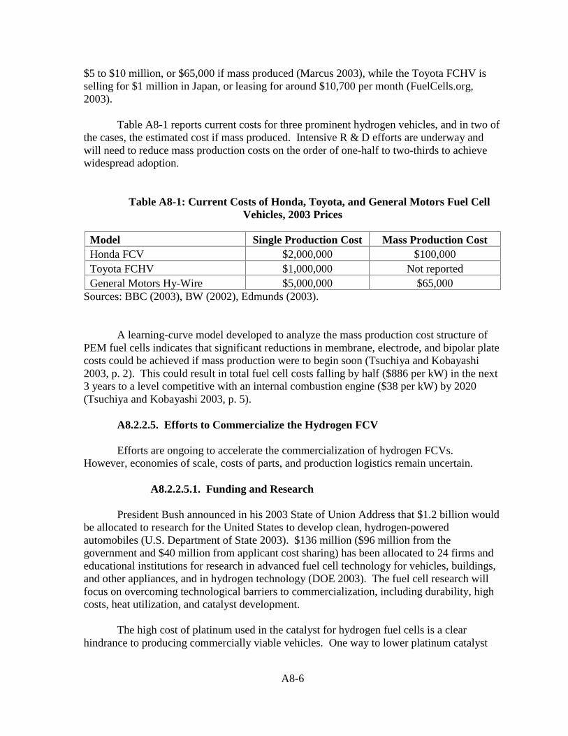
A8-6

$5 to $10 million, or $65,000 if mass produced (Marcus 2003), while the Toyota FCHV isselling for $1 million in Japan, or leasing for around $10,700 per month (FuelCells.org,2003).

Table A8-1 reports current costs for three prominent hydrogen vehicles, and in two ofthe cases, the estimated cost if mass produced. Intensive R & D efforts are underway andwill need to reduce mass production costs on the order of one-half to two-thirds to achievewidespread adoption.

Table A8-1: Current Costs of Honda, Toyota, and General Motors Fuel CellVehicles, 2003 Prices

Model Single Production Cost Mass Production CostHonda FCV $2,000,000 $100,000Toyota FCHV $1,000,000 Not reportedGeneral Motors Hy-Wire $5,000,000 $65,000

Sources: BBC (2003), BW (2002), Edmunds (2003).

A learning-curve model developed to analyze the mass production cost structure ofPEM fuel cells indicates that significant reductions in membrane, electrode, and bipolar platecosts could be achieved if mass production were to begin soon (Tsuchiya and Kobayashi2003, p. 2). This could result in total fuel cell costs falling by half ($886 per kW) in the next3 years to a level competitive with an internal combustion engine ($38 per kW) by 2020(Tsuchiya and Kobayashi 2003, p. 5).

A8.2.2.5. Efforts to Commercialize the Hydrogen FCV

Efforts are ongoing to accelerate the commercialization of hydrogen FCVs.However, economies of scale, costs of parts, and production logistics remain uncertain.

A8.2.2.5.1. Funding and Research

President Bush announced in his 2003 State of Union Address that $1.2 billion wouldbe allocated to research for the United States to develop clean, hydrogen-poweredautomobiles (U.S. Department of State 2003). $136 million ($96 million from thegovernment and $40 million from applicant cost sharing) has been allocated to 24 firms andeducational institutions for research in advanced fuel cell technology for vehicles, buildings,and other appliances, and in hydrogen technology (DOE 2003). The fuel cell research willfocus on overcoming technological barriers to commercialization, including durability, highcosts, heat utilization, and catalyst development.

The high cost of platinum used in the catalyst for hydrogen fuel cells is a clearhindrance to producing commercially viable vehicles. One way to lower platinum catalyst

A8-7

levels is to construct the catalyst layer with the highest possible surface area. The LosAlamos National Laboratory (LANL) has developed a fabrication process for fuel cellmembrane electrode assemblies with reduced platinum loading that decreases the cost of thecatalyst by 90 percent (LANL 2000).

Danish Power Systems has developed a PEM fuel cell stack system that meetsautomaker requirements for an operating temperature that runs at up to 200 degrees C and iseasier to cool than the low-operating ones that run below 100 degrees C. The membrane ofeach PEM fuel cell is made of PBI, a thermally high resistant material that possesses uniqueproperties that increase efficiency and costs less than the traditional Nafion (Bjerrum 2003).

Hydrogen technology research is also heavily funded to overcome the technicalbarriers of storage capacity and cost, along with improving life cycle cost and energyefficiency and improving methods of hydrogen production (Rose 2003a). For example, DOEhas funded projects to develop methods to safely store hydrogen to enable at least a 300-milevehicle range, which it considers a critical requirement for successful vehiclecommercialization.

A8.2.2.5.2. Federal FCV Pilot Study

The federal government is currently involved in a ten-year program to help facilitatethe commercialization of fuel cell technology (Rose 2003b). It has been proposed that theSecretary of Energy lead a cooperative effort among federal agency fleet operators andprivate-sector FCV companies in a cost-shared program to purchase, operate and evaluateFCVs in integrated service for federal fleets to demonstrate their commercial viability in arange of climates, duty cycles, and operating environments.

This $495 million program includes two phases to reach the goals of this pilot-fleetdemonstration. Phase I runs from 2004-2007, and includes the purchase of 500 passengervehicles, 500 Department of Defense (DOD) vehicles, 100 transit buses, 100 school busesand 20 fueling stations, demonstrating a range of fuels and fueling strategies. Phase II runsfrom 2008 to 2011, when the federal government would meet 50 percent of its civilianvehicle fleet needs with fuel cell vehicles, or purchase 5,000 passenger vehicles annually.During this phase, the DOD and the Cabinet secretaries would set their own targets on thenumber of military vehicles or mobile equipment and specialty vehicles needed.

A8.2.2.5.3. Proposed Tax Incentives

The Breakthrough Technologies Institute, Inc. recently published a report thatincluded a FCV ten-year market entry support plan (Rose 2003b). The report recommendeda short-term consumer-based tax incentive that would reduce the incremental cost for earlyadopters and help the FCV industry build production capacities to reach economies of scale.It suggested that Congress continue the existing $4,000 tax credit system for qualifying fuelFCVs.

A8-8

In addition, the report proposed that Congress enact a tax credit for the installation offuel-cell re-fuelling infrastructure that is accessible to the public. These re-fuelling programswould also include a direct tax credit of 50 percent of the cost of the station up to $150,000.The report also proposed that fuel for FCVs be offered a $.30 per gasoline-of-gallon-equivalent tax credit in 2003, $.40 per gallon in 2004 and $.50 per gallon from 2005 to 2012.

A8.2.3. Hydrogen Fuel Distribution Infrastructure

A major challenge to the viability of the hydrogen economy is the necessity of ahydrogen fuel distribution infrastructure. Three restrictions describe its current state:consumers will not purchase FCVs without adequate fueling stations, manufacturers will notproduce vehicles without real demand, and fuel providers will not build fueling stationswithout vehicles to fuel. To overcome what has been characterized as a chicken-or-eggproblem, Ogden (1999, p. 268) suggests that distributors initially piggyback on existingenergy infrastructure, e.g. building production facilities at fueling stations, thereby avoidingthe need to build an extensive pipeline system. Alternatively, Melaina (2003, p. 753)suggests a phased approach beginning with building small capacity fueling stations that onlystore hydrogen, until greater demand is built, a strategy endorsed by NRC (2004, pp 2-9 to2-10). Either way, the development of a distribution infrastructure that will support cost-effective refueling will be an investment challenge, probably more for fuel suppliers than forvehicle suppliers. The fact that the two are distinct businesses may complicate the challenge.

A8.2.4. Viewpoints on the Prospects of the Hydrogen FCV

Current views on the development of hydrogen FCVs vary greatly. On one hand,environmentalists seem to welcome the possibility of a clean fuel, automakers appear to viewthis as a niche market with gains to be made, and the government seeks to reduce foreign oildependence. The Allied Business Intelligence group (ABI) forecasts that the global fuel cellvehicle market will number 800,000 by 2012 (Wengraff 2003). Other groups, however,believe research in hydrogen power is a political effort to allow fossil fuel dependentcompanies to sustain their markets. It is claimed that funding some research now providesthe appearance of a change in the energy industry while extending the time that the countrywill be fossil-fuel dependent. In between are those who suggest that comparing hydrogenenergy, given its current economic and scientific uncertainties, with other alternatives doesnot give a clear answer about the promise of hydrogen.

Support from the government has come in the form of DOE’s FY2004 budgetproposal for a $123 million increase in federal research support. David Cole, director of theCenter for Automotive Research suggests that, “…there is a very high rate of improvement intechnology and with strong leadership, maybe, just maybe they can do it” (Flint 2003). Apoll sponsored by Millennium Cell, Inc. and US Borax, Inc. in April 2003 that surveyed1,006 Americans age 18 or older found 85 percent of Americans willing to try hydrogen-fueled vehicles, while only 12 percent expressed an unwillingness to try the vehicles (EERE2003).

A8-9

At the other end of the spectrum, the National Hydrogen Energy Roadmap and othersources suggest that the Bush administration has been working to ensure that hydrogenproduction will remain fossil fuel-dependent and dirty, as 90 percent of all hydrogen wouldbe refined from oil, coal and natural gas while the remaining 10 percent will be cracked fromwater using nuclear energy. The process of producing the fuel cells from hydrocarbons willcontinue America’s dependence on fossil fuels and still emit carbon dioxide, the primarycause of global warming (CNN 2003; Lynn 2003; ITS 2002; Kolber 2003; Hunt 2002).

In between are those who think that given the major scientific and economicimprovements necessary to be successful, funds could be better used to focus on more viableoptions (Popely 2001; Tromp et al. 2003). David Cole warns that fuel cells may notultimately be the solution to reducing fossil-fuel dependence, since hybrid electric vehicles,diesels, or a new technology could prove more cost-effective (Flint 2003). The NaturalResources Defense Council contends that funding of the hydrogen car cuts the budget forother federal research into clean energy by $47 million (Rosenbaum 2003).

A8.3. Considerations for Large-Scale Hydrogen Production

Should natural gas prices rise, electrolysis of water may become the primaryhydrogen production method to meet the needs of a growing FCV market. Kruger’s (2000)analysis of electric power requirements suggests that by 2010, 165 GW of additional capacitywould be needed to meet increased hydrogen demand from the use of 20,000 fuel cellvehicles, beyond the requirements to meet other sources of demand growth. This wouldamount to a 20 percent increase over current capacity.

While renewable energy sources can be used to produce hydrogen, those fail to meetthe scale demanded by industry: using wind power would require as many as 640,000windmills occupying 71,000 square miles (about the size of Indiana and Ohio); powergeneration using biomass would require four times as much plant material as U.S. farmerscurrently grow; the solar option would require $4.8 trillion worth of solar panels andequipment occupying 3,000 square miles (NEI 2003). Reducing these estimates by one-halfwould not materially relax the limitations to renewables supplying hydrogen at an industrialscale.

Sufficient domestic coal exists to fire electrical plants to provide both the electricityand the hydrogen needed for several hundred years. Building new power plants required tomeet this demand would be a large—but not infeasible—task, but coal-fired power plantsgenerate carbon dioxide and other emissions. Without expensive emission control methods,coal plants would simply discharge these substances into the atmosphere at a differentlocation from automobiles, increasing carbon emissions on balance. Such a strategy woulddo little to combat pollution and global warming or harness the environmental benefits ofhydrogen. Production of hydrogen using steam methane reforming is capable of reducingcarbon emissions on balance, but only modestly. Substituting hydrogen for gasoline invehicular transportation would reduce carbon emissions from the gasoline but would involve

A8-10

carbon emissions from the production of the hydrogen. When the reductions in vehicleemissions from substituting hydrogen for gasoline are balanced against the increases inemissions from the gas-steam methane reforming (SMR) units producing the hydrogen, thesubstitution would reduce about 18 percent of the carbon emitted per gallon of gasoline,based on calculations with information from Honda (2003), EPA (2003), and ORNL (2003).

Nuclear power plants, on the other hand, can generate the heat necessary to producehydrogen through a variety of alternative processes. Nuclear power produces no greenhousegases. Nuclear energy is the only energy source that produces no air emissions but still hasenough production potential to generate the required quantities of hydrogen.

A8.4. Hydrogen Production Techniques

Several methods exist for producing hydrogen, all of which involve extracting purehydrogen gas from hydrogen-containing compounds. This section considers how thesetechniques can be used in conjunction with the outputs of nuclear energy—electricity andheat—to economically create hydrogen.

Presently hydrogen is manufactured almost exclusively by steam methane reforming,which uses methane as a feedstock. Steam methane reforming uses heat, but it releasescarbon dioxide as a by-product. Carbon-free methods can extract hydrogen from water usingenergy by electrolysis and thermo-chemical cycles (Forsberg 2003, p. 1075). Electrolysistechniques are commercially available but are used only at small scales currently, and theyuse electricity rather than heat. The thermo-chemical cycles could be powered by advancednuclear reactors.

A8.4.1. Steam Methane Reforming

Steam methane reforming is a two-step process that results in the production ofcarbon dioxide and hydrogen. In the conventional process, natural gas is simultaneouslyused as a source of hydrogen and is burned to produce heat to drive the reaction at atemperature of 800 to 900ºC. It remains the most economical method of producinghydrogen. Typical thermal efficiencies for steam reforming processes are about 70 percent.However, as has been noted, this process merely relocates where carbon dioxide is emittedrather than contributing to greenhouse gas reductions. Molburg and Doctor (2003) report ona simulation of hydrogen production via a steam methane reforming process, without andwith carbon sequestration. At a methane price of $2.85 per MMBtu, the process couldproduce hydrogen at a cost of $0.83 per kg while releasing 1,366 tons of CO2 per day.Capturing CO2 would increase the cost by 35 percent, to $1.12 per kg.

It is possible that the amount of natural gas required for the process can be greatlyreduced by utilizing the heat from nuclear reactors. The necessity to transport heat hasresulted in a number of problems such as diffusion of product and the creation of impurities.The Japan Atomic Energy Research Institute (JAERI) is leading the current research on

A8-11

steam reforming in combination with a nuclear reactor. The institute has developed a heatexchanger type of nuclear reactor for the reforming process that has minimized many of theoperational issues. Since this uses standard hydrogen production technology it represents theonly near-term nuclear-hydrogen technology (Forsberg 2003, p. 1075).

A8.4.2. Electrolysis

Electrolysis, while a mature technology, has been used historically to produce purehydrogen only in small quantities. Electrolysis is essentially the splitting of water moleculesby electricity. Electrodes, a cathode and an anode, placed in an alkaline solution drive themovement of electrons. Hydrogen forms at the cathode and oxygen at the anode.

While current electrolyzers have efficiencies approaching 85 percent or better,electrolysis is not competitive for large-scale production of hydrogen, given its capital costand electricity consumption. Current capital costs are estimated to be near $600 per kW(Forsberg 2003, p. 1075). Average electricity consumption is 4.5 kWh per cubic metres ofhydrogen, (Kruger 2000, p. 128).

A possibility for improving the economic conditions for electrolysis would be forelectricity generators and hydrogen production facilities to agree to use off-peak electricityfor the electrolysis production (Crosbie and Chapin 2003, p. 3). Several studies have shownthat when electricity is cheap enough, for example at off-peak rates of $2 to $3 permegawatt-hour, hydrogen might be produced at a price competitive with the price of gasolineor diesel fuel. NRC (2004, p. 5-16) concludes that electricity prices will be critical to the useof electrolysis for hydrogen production.

A8.4.3. Thermo-Chemical Cycles

Thermo-chemical cycle water-splitting processes offer the potential for makinghydrogen at temperatures in the range of 700 to 900ºC. This process is considered to be theleading long-term option for hydrogen production (Crosbie and Chapin 2003, p. 9). Thebasic cycle involves the thermal decomposition of water into hydrogen and oxygen using anionic solution to mediate the reaction.

The most promising of these cycles are the calcium-bromine process and the sulfur-iodine process. Currently, neither of these thermo-chemical processes has progressed to thepoint of commercial viability, perhaps partly because there has not been the economicincentive to do so. Recently, however, interest in environmental benefits and energyindependence has increased attention to these methods. Recent estimates indicate thatthermo-chemical production costs could be 60 percent of current electrolysis costs usingnuclear reactors dedicated to hydrogen production (Forsberg 2003, p. 1075).

Thermo-chemical processes would be conducted from nuclear reactors dedicated tohydrogen production. The greater proportion of the heat generated by the reactor would beused for the hydrogen production, but the waste heat could be used to power a steam turbinewhich would generate electricity that could be sold outside the hydrogen production facility.

A8-12

In this production process, the ability to sell electricity from a hydrogen facility would reducethe cost of hydrogen production.

A8.5. Conclusion

Extensive market penetration of the fuel cell vehicle would greatly increase thedemand for hydrogen. Current costs of those vehicles, however, are not competitive withICE vehicles, particularly because of the materials used in the fuel cell membrane.Companies and government agencies are funding research and investment to reduce thesecosts. Near-term prospects for market penetration remain difficult to assess.

Should the demand for hydrogen burgeon with new demands from the transportationsector, there are a number of process options for producing large amounts of hydrogen for afuture hydrogen economy. The maturity of these various techniques differs, with some of themost efficient and useful processes still working their way through development. Nuclearpower, because of its zero air emissions, offers potential synergies and cost efficiencies forthe production of hydrogen.

A8-13

References

Arthur D. Little, Inc. (2001) “Cost Analysis of Fuel Cell System for Transportation: 2001System Cost Estimate.” Report to U.S. Department of Energy. Cambridge, Mass.: ArthurD. Little, Inc., August.

Argonne National Laboratory (ANL). (2003) “Meeting U.S. Transportation Needs in theHydrogen Economy.” Retrieved December 13, 2003 from the World Wide Web:http://hydrogen.anl.gov/pdfs/meeting_transportation_needs.pdf.

British Broadcasting Corporation (BBC). (2003) “An Overview of the GM Hy-Wire Car”Retrieved from the World Wide Web: http://www.bbc.co.uk/dna/place-london/A1143505.

Business Week (BW). (2002) “Commentary: Fuel Cells: Japan's Carmakers Are FlooringIt”. Retrieved from the World Wide Web:http://www.businessweek.com/magazine/content/02_51/b3813084.htm.

Bjerrum, N.J. (2003) “Danish Breakthrough for the Next Generation of PEM Fuel Cells.”Retrieved December 13, 2003 from the World Wide Web:http://www.fuelcellsworks.com/Supppage247.html.

Cable News Network (CNN). (2003) “Bush Hydrogen Initiative Furls Debate.” RetrievedAugust 2003 from the World Wide Web:http://www.cnn.com/2003/ALLPOLITICS/02/07/hydrogen.vision.ap/.

Crosbie, L. and D. Chapin. (2003) “Hydrogen Production by Nuclear Heat.” MPRAssociates, Inc., Alexandria, Va.

Davis, C., B. Edelstein, B. Evenson, A. Brecher, and D. Cox. (2003) “Hydrogen Fuel CellVehicle Study,” Panel of Public Affairs & American Physical Society, June 12. RetrievedSeptember 2003 from the World Wide Web:http://www.aps.org/public_affairs/popa/reports/fuelcell.pdf.

Doctor, Richard D. (2002) “STAR-H2: A Calcium-Bromine Hydrogen Cycle Using NuclearHeat.” Argonne National Laboratory. Retrieved from the World Wide Web:http://hydrogen.anl.gov/pdfs/doctor-0302.pdf.

Edmunds.com. (2003). “Honda’s Pollution-Free Car”. Retrieved from the World WideWeb: http://www.edmunds.com/advice/specialreports/articles/100335/article.html, July 2003.

Flint, J. (2003) “The Hydrogen Car?” Ward’s Auto World. Retrieved August 2003 from theWorld Wide Web:http://www.wardsauto.com/magazinearticle.asp?magazinearticleid=170599&magazineid=50&siteID=26&siteID=26&releaseid=11107&mode=print.

A8-14

Forsberg, Charles W. (2003) “Hydrogen, Nuclear Energy, and the Advanced High-Temperature Reactor,” International Journal of Hydrogen Energy 28: 1073-1081.

FuelCells.org. (2000). “Fuel Cell Vehicles (from Auto Manufacturers).” The Online FuelCell Information Center. Retrieved September 2003 from the World Wide Web:http://fuelcells.org/fcfaqs.htm#efficient.

General Motors (GM). (2002) “GM Hy-Wire: Major Step Forward in Reinventing theAutomobile.” Retrieved December 2003 from the World Wide Web:http://www.gm.com/company/gmability/environment/products/fuel_cells/hywire_081402.html.

Honda Motors. (2002) “Honda FCX Fact Sheet.” Retrieved July 2003 from the WorldWide Web: http://hondacorporate.com/fcx/press/5.html.

Honda Motors. (2003) “Honda FCX Overview.” Retrieved December 2003 from WorldWide Web: http://www.hondacorporate.com/fcx/specs.html.

Hunt, E. (2002) “Fuel Cell or Fuel Efficiency?” The Christian Science Monitor, January 18.Retrieved August 2003 from the World Wide Web:http://www.csmonitor.com/2002/0118/p11s02-coop.html.

Institute of Transportation Studies (ITS). (2002) “Is Bush’s Freedom-Car Hot Air?”Retrieved August 2003 from the World Wide Web:http://www.its.berkeley.edu/publications/ITSReviewonline/july2002/freedomcar.html.

Kolbert, Elizabeth. (2003) “The Car of Tomorrow,” The New Yorker, August 11, pp. 36-40.

Kruger, Paul. (2000) “Electric Power Requirement in the United States for Large ScaleProduction of Hydrogen Fuel,” International Journal of Hydrogen Energy 25: 1023-1033.

Los Alamos National Laboratory (LANL). (2000) “Fuel Cells at Los Alamos.” RetrievedJuly 2003 from the World Wide Web:http://fuelcells.org/FY%202004%20Budget%20Rev1.pdf.

Lynn, B.C. (2003) “Hydrogen’s Dirty Secret,” Mother Jones, May/June. Retrieved August2003 from the World Wide Web:http://www.motherjones.com/news/outfront/2003/19/ma_375_01.html.

Markus, Frank. (2003) “Driving Impression: GM Hy-Wire,” Car and Driver Magazine,March. http://www.caranddriver.com/article.asp?section_id=19&article_id=4185, July 2003.

Massachusetts Institute of Technology (MIT) and Materials System Laboratory (MSLL).(2003) “Proposal for the Establishment of an Alternative Fuel Economics Laboratory.”

A8-15

Retrieved August 2003 from the World Wide Web:http://msl1.mit.edu/msl/meeting_04192001/prz_pdf/ibaron.pdf.

Melaina, Marc W. (2003) “Initiating Hydrogen Infrastructures: Preliminary Analysis of aSufficient Number of Initial Hydrogen Stations in the U.S,” International Journal ofHydrogen Energy 28: 743-755.

Molburg, John C., and Richard D. Doctor. (2003) “Steam Methane Reforming—CO2 LifeCycle Analysis.” Draft, FWP 00FE49497. Argonne, Ill.: Argonne National Laboratory,February 1.

Morita, Y. (2003) “Development and Diffusion of Fuel Cell Powered Automotive Vehiclesand Its Impact.” Tokyo: The Energy Data and Modeling Center, The Institute of EnergyEconomics.

National Research Council (NRC). (2004) The Hydrogen Economy: Opportunities, Costs,Barriers, and R&D Needs. Washington, D.C.: National Academies Press.

Nice, K. (2003) “How Fuel Cells Work.” Retrieved December 2003 from the World WideWeb: http://auto.howstuffworks.com/fuel-cell.htm/printable.

Nuclear Energy Institute (NEI). (2003) “The Hydrogen Economy and Nuclear Energy.”Retrieved December 2003 from the World Wide Web:http://www.nei.org/index.asp?catnum=2&catid=265.

Oak Ridge National Laboratory (ORNL). (2003) Carbon Dioxide Information AnalysisCenter. Oak Ridge, Tenn.: Environmental Sciences Division, Oak Ridge NationalLaboratory. Retrieved December 2003 from World Wide Web:http://cdiac.esd.ornl.gov/pns/faq.html.

Ogden, Joan. (1999) “Prospects for Building a Hydrogen Energy Infrastructure,” AnnualReview of Energy and Environment 24: 227-280.

Ogden, Joan. (2002) “Hydrogen: The Fuel of the Future?” Physics Today 55: 69-76.

Popely, R. (2001) “H2 Oh: Carmakers Move Toward Hydrogen Fuel Cells.” ChicagoTribune. August 12.

Rose, R. (2003a) “FY 2004 Budget Proposals for Fuel Cells and Hydrogen.” U.S. Fuel CellCouncil. Retrieved from the World Wide Web: http://fuelcells.org.

Rose, R. (2003b) “Fuel Cells and Hydrogen: The Path Forward.” Washington, D.C.:Breakthrough Technologies Institute, Inc.

A8-16

Rosenbaum, David. (2003) “How Would You Cut the Federal Budget?” New York Times,section 4, p. 3, February 9.

Schultz, Kenneth R. (2003) “Use of the Modular Helium Reactor for HydrogenProduction.” San Diego: General Atomics. Retrieved December 2003 from the World WideWeb: http://www.world-nuclear.org/sym/2003/pdf/schultz.pdf.

Toyota Motors. (2002) “Toyota Delivers First Two, Market-Ready-Zero-Emission-CertifiedHydrogen Fuel Cell Vehicles.” Retrieved July 2003 from the World Wide Web:http://www.toyota.com/about/news/environment/2002/12/02-1-fuelcell.html.

Thomas, S., and M. Zalbowitz. (2003) “Fuel Cells- Green Power.” Los Alamos, N.M.: LosAlamos National Laboratory. Retrieved from World Wide Web:http://education.lanl.gov/resources/fuelcells/fuelcells.pdf.

Tromp, Tracey K., Run-Lie Shia, Mark Allen, John M. Eiler, Y. L. Yung. (2003) “PotentialEnvironmental Impact of a Hydrogen Economy on the Stratosphere,” Science 300: 1740-1742.

Tsuchiya, H., and O. Kobayashi. (2003) “Mass Production Cost of PEM Fuel Cell byLearning Curve,” forthcoming in International Journal of Hydrogen Energy.

U.S. Department of State. (2003) “Transcript: President Bush’s State of the UnionAddress.” Retrieved December 2003 from the World Wide Web:http://www.usembassy.org.qa/usisdoha/sou03.htm.

U. S. Department of Energy (DOE). (2003) “Energy Department Awards $75 Million forAdvanced Hydrogen Fuel Cell R&D.” Retrieved December 2003 from the World Wide Web:http://www.energy.gov/engine/content.do?PUBLIC_ID=13801&BT_CODE=PR_PRESSRELEASES&TT_CODE=PRESSRELEASE.

U. S. Department of Energy, Office of Energy Efficiency and Renewable Energy (EERE).(2003) “Fact of the Week: Americans Willing to Try Hydrogen-Fueled Vehicles.” RetrievedNovember 2003 from the World Wide Web:http://www.eere.energy.gov/vehiclesandfuels/facts/2003/fcvt_fotw274.shtml, accessed.

U.S. Environmental Protection Agency (EPA). (2003) “Light-Duty Automotive Technologyand Fuel Economy Trends: 1975 through 2003.” Data from Appendix F. RetrievedDecember 2003 from World Wide Web: http://www.epa.gov/otaq/fetrends.htm.

Weiss, M. A., J. Heywood, A. Schaefer, and V. Natarajan. (2003) “ComparativeAssessment of Fuel Cell Cars.” Cambridge, Mass.: Massachusetts Institute of Technology,February.

A8-17

Wengroff, J. (2003) “Fuel Cell Vehicles to Number 800,000 by 2012, According to ABI.”Allied Business Intelligence. Retrieved July 2003 from the World Wide Web:http://www.abiresearch.com/pdfs/afc02pr3.pdf.

A8-18

A9-1

Appendix A9. ENERGY SECURITY

Summary

Nuclear power could provide energy security benefits as a potential source ofhydrogen to replace oil in the transportation sector and more generally as a substitute for gas-generated electricity.

Energy security has been discussed primarily in connection with oil and the politicalinstability of the Middle East. A direct link to electricity is limited by the small amount ofelectricity produced using oil. One way by which nuclear electricity generation could berelated to oil security is via cogeneration of hydrogen for widespread use in transportation. Ifcogeneration with nuclear power is the least expensive source of hydrogen, it wouldcontribute to speeding the adoption of hydrogen vehicles, reducing dependence on oil.

Currently the United States imports about 4 percent of its natural gas in the form ofLNG, but this percentage could grow if substantial new capacity is devoted to gas-firedproduction and if North American gas production expands only very sluggishly. Asinternational trade in LNG becomes more extensive and the United States participates in itmore deeply, this energy security linkage could become more important.

The effect of foreign dependence on gas is influenced by differences between worldoil and gas markets. The world natural gas market is less unified than the world oil market.Price increases in one part of the world are not as quickly and completely transferred to othercountries as with oil, as shown by analysis of natural gas prices for over thirty countries.Results show high correlations of gas price movements within Europe, but low correlationsbetween European countries and non-European countries. Canadian, Mexican and U.S. gasprices are highly correlated with one another, but none of these North American countries’prices is highly correlated with either European or Asian prices. Gas prices in Taiwan andJapan, both of which import considerable amounts of LNG from Indonesia and Malaysia, arehighly correlated, as would be expected in that regional market. However, their gas priceswere essentially uncorrelated with gas prices in North America or Europe.

This balkanization of natural gas prices around the world suggests that whilecountries may be subject to economic repercussions from gas supply shocks in their ownregions, they tend to be insulated from supply shocks in other regions.

Gas does not pose as great an energy security threat as oil, but, still, nuclear powergeneration capacity could become a significant defense against regional gas supplyinterruptions. Interruptions could extend increasingly to offshore sources, given thelikelihood of only limited additional imports from Canada and Mexico.

Projections of gas prices are reported in Chapter 7. Recent projections from a numberof models have forecast gas prices in 2020 to be slightly below their levels in 2000, inconstant dollars. However, in the recent period of gas price volatility and uncertainty about

A9-2

supplies, EIA revised its 2020 forecast, published in the Annual Energy Outlook 2004 (AEO2004), upward by 15 percent, to be 11 percent higher than in 2000 and 20 percent aboveprices in 2005. The current EIA forecast predicts the average wellhead price for the lower 48states to vary from $3.62 per MMBtu in 2005 to $4.51 per MMBtu by 2025 (in 2003 dollars).

Given a national interest in encouraging greater reliance on nuclear power (seeNEPDG 2001, pp. 5-15—5-17; Abraham 2004; DOE and Nuclear Power Industry 2004,Foreword; Bush 2004), the question arises: What are the criteria for deciding whatproportion of new baseload capacity should be devoted to nuclear power? The answer to thisquestion depends partly on the variety of 21st century uncertainties that the nation needs to beprepared for. Uncertainties affecting demands for nuclear power include foreign policy, theenvironment, natural gas and other significant events. As only one example, a probabilityexists that environmental events will substantially increase the cost of producing electricitywith gas and coal relative to the cost of nuclear generation, increasing the demand for nucleargeneration. Maintaining some nuclear capacity now could avoid the costly and lengthyadjustment costs of gearing up a nuclear industry that might otherwise be in a run-downcondition. To do so could be a prudent procedure as part of making optimal decisions in theface of an uncertain future. A decision model is developed that compares the costs of beingprepared for such events with the expected benefits if the risk materializes. Using thismodel, the study develops a numerical example of the amount of new capacity to devote tofossil and nuclear electrical generation. In this example, 25 percent of new capacity wouldbe nuclear. Further research along these lines could greatly aid future decisions.

A9-3

Outline

A9.1. Introduction: What Energy Security Is

A9.2. Oil and Energy Security

A9.2.1. The Track Record with OilA9.2.2. A Unified World Oil MarketA9.2.3. Concentration of Oil ReservesA9.2.4. Oil Price Shocks and Gas-Fired Electricity Generation

A9.3. The Present and Future of Natural Gas

A9.3.1. The Recent Price Increases and Forecasts for the FutureA9.3.2. U.S. Natural Gas Consumption and Longer-Term Gas Supplies in the

Continental United States and CanadaA9.3.3. Gas Imports—LNGA9.3.4. Vulnerability of Gas to Price ShocksA9.3.5. The World Gas MarketA9.3.6. Implications for Natural Gas as an Energy Security Issue

A9.4. Energy Security Implications for Nuclear Power

A9.4.1. Sources of UncertaintyA9.4.2. Toward Modeling UncertaintyA9.4.3. Appendix

References

A9-4

A9.1. Introduction: What Energy Security Is

Energy security is to be distinguished from national security in the military sensealthough sufficiently dire scenarios could envision supply reductions severe enough tocompromise military capabilities. Of more immediate concern is the possibility that sharp,short-lived events affecting energy could damage the economy. This has been the experienceof the United States and the rest of the world since the 1970s, and even earlier, in the face ofunexpected oil supply interruptions and consequent price shocks.

This appendix addresses the potential for nuclear power to lessen energy securityvulnerabilities. The next section examines the energy security issues involved in the oilmarket. Section A9.3 considers the routes by which nuclear power could contribute toenhanced energy security. Natural gas used for electricity generation provides a possible linkbetween nuclear power and energy security. Section A9.4 examines the natural gas marketfor characteristics that could make gas an energy security risk.

A9.2. Oil and Energy Security

Section A9.2.1 describes the recent oil price shocks, Section A9.2.2 characterizes thesignificance of the unity of the world oil market, and Section A9.2.3 notes the importance ofthe geographic concentration of world oil reserves.

A9.2.1. The Track Record with Oil

The recent history of the world oil market is one of recurrent shocks. Fringe suppliershave responded to the price increases but with lags of up to several years. Real oil priceshave come back down in each case, to pre-OPEC levels, dramatically in the 1985 pricecollapse. After a few years, it seems as though the world’s expectations have adjusted tothink that oil can no longer be an economic threat, and the cycle repeats itself. Economicdamages result from the price shocks.

The oil price shocks of 1973 to 1974, 1979 to 1980, and 1990 to 1991 werecontributors to the ensuing recessions. In each case, a shock to supply resulted in a sharpprice rise—an unprecedented price rise in the first of these three episodes. The 1973 to 1974episode was the result of deliberate output restriction by the Organization of PetroleumExporting Countries (OPEC). Much of the world had considerable difficulty indistinguishing what turned out to be a temporary rise in the oil price from a transition topermanently higher prices of all energy, and it took several years for the world economy torecognize the transience of the price regime. Research on a myriad of energy-using and –producing technologies began in the mid-1970s, and the price levels, and their expectedlengthy duration prompted equally enthusiastic oil exploration. Both endeavors were largelysuccessful, and prices had begun to come down just as the second great price shock occurred.

A9-5

The 1979 to 1980 events began with supply interruptions from Iran during theKhomeini revolution and were supplemented with further interruptions when Iraq took theopportunity to attack Iran in 1980. Both events fortuitously interrupted oil production andshipments from both Iran and Iraq, and the slack was not picked up by the OPEC swingproducer, Saudi Arabia. Both the Iranian Revolution and the beginning of the Iran-Iraq Wartook the world by surprise, and the political and military consequences were uncertain forwell over a year. By 1982, the United States was well into recession. The politicaluncertainties of the Persian Gulf disturbances were resolved over the next few years, and theenergy R&D and oil exploration sparked by the OPEC embargo’s price shock reachedfruition. By 1985, the world supplies of oil had greatly increased, and at the same time oilintensities of all types of industrial production had begun to fall significantly. The result wasthe 1985 oil price collapse.

Iraq’s invasion of Kuwait in August 1990 cut off Kuwaiti oil supplies, and for overtwo months the integrity of Saudi supplies was in question. After some negotiation, SaudiArabia compensated for much of the lost production, but Iraq’s military action had caught theworld by surprise and the military uncertainty lasted until the allied invasion began in mid-January 1991. Prices rose by 50 percent overnight and remained near that level until thebeginning of the allied attack. The economic uncertainties of the situation were resolvedrapidly, but the United States, which had been on the brink of recession prior to August 1990,fell into a full-scale recession with the push from the oil price shock.

OPEC has demonstrated some cartel power in recent years, but it has been temperedby the reserve army of fringe producers that has emerged as a consequence of the earlier oilprice shocks. While Saudi Arabia remains the swing producer—the cartel leader—its pricepower appears to be weaker, although a few random events around the world could put itback in the driver’s seat for a time.

Oil has clearly been an economic problem. Hamilton (1983) presented evidence thatthe post-1973 relationship between oil prices and U.S. recessions went back to the late 1940s.Despite occasional suggestions that these oil price shocks were only fortuitously associatedwith the ensuing recessions, the preponderance of the evidence indicates that the oil supplyshocks have indeed had major recessionary impacts (Jones et al. 2004).

A9.2.2. A Unified World Oil Market

While the dynamics of oil prices, with its storability, are interesting, it is sufficient forpresent purposes to emphasize the relative unity of the world oil market. Oil can be shiftedaround the world at relatively low cost by tankers and low-pressure pipelines in response torelatively small differentials in price. Price differentials will always exist according to thephysical qualities of oil and the expense of refining them at particular facilities, but changesin the price of one grade of oil in one location in the world are invariably followed closely bynearly parallel changes in the prices of all other grades of oil all over the world.

A9-6

The unity of the world oil market leaves all countries facing similar price movementswhen a sizeable supply shock emerges in any part of the world. This is an importantcharacteristic of the economics of oil. A corollary to this consequence of a unified world oilmarket is that if a single country were to substitute entirely away from oil, its economy couldstill be vulnerable to a world downturn caused by an oil price shock to countries still usingoil. This latter consequence is a more remote event than the inexorability of oil pricechanges occurring relatively uniformly worldwide, but it remains a consideration in theeffectiveness of longer-term energy strategies.

A9.2.3. Concentration of Oil Reserves

As is well known, world oil reserves are extremely heavily concentrated in arelatively small region of the world—the Persian Gulf. Despite discoveries in the North Seaand across Central Asia, an estimated 60 to 75 percent of known reserves remain in a fewcountries surrounding the Persian Gulf, although current production is somewhat lessconcentrated. This concentration of reserves, and their ownership by those countries’governments, gives considerable market power to those countries.

In addition to the physical concentration of oil reserves in a small number ofcountries, the political instability of the region adds an additional element of unpredictabilityto supplies and prices. The Iranian Revolution did not intentionally take Iran’s oil productionoff line, but that occurred as a concomitant to the temporary disorder. The prospect ofpolitical turmoil elsewhere in the region cannot be fully discounted. Temporary disruptionsto its oil fields would represent a major reduction in world supplies that could not be made upquickly by increased production in other regions.

Both characteristics—geographical concentration and concentration in an unstableregion—contribute to the volatility of the world oil market.

A9.2.4. Oil Price Shocks and Gas-Fired Electricity Generation

To date, energy security issues for the United States have involved oil. Very little oilis used in the generation of electricity in the United States. Among industrial countries, onlyItaly continues to have a substantial fraction of its generation capacity in oil-fired units. Oilis used primarily in the transportation sector, which also uses very little electricity. In viewof the tenuous linkage between electricity and oil, does nuclear power have a role in energysecurity? One possible link is the use of natural gas in electricity.

A link between oil and electricity through the use of natural gas in electricitygeneration would be a near-term link, one that could operate presently. Oil and natural gasare substitutes in some industrial uses, so an oil price shock could raise natural gas pricesfacing electric utilities as well as industrial gas consumers. That would raise electricityprices. The substitutability between coal and oil is currently lower than that between oil andgas because of less extensively overlapping uses.

A9-7

The extent of actual substitutions between oil and gas in industrial uses, which wouldbe the driver of cost increases for gas-fired electricity generation, would probably depend onthe character of the oil price increase. A short, sharp price shock such as the industrial worldhas experienced several times since the early 1970s, could fail to motivate industrial oilconsumers to switch to gas if the oil price is expected to fall rapidly and the switch-over costswere high relative to the cost of curtailing production for an expected short period.Nonetheless, a two- or three-year-long period of elevated oil prices would see natural gasprices rise in response, to keep their prices per MMBtu roughly equal. A longer-term,probably slower, oil price increase such as would be associated with dwindling worldwidereserves rather than a cartel action, would certainly be matched with parallel gas priceincreases.

A9.3. The Present and Future of Natural Gas

The potential link between natural gas and nuclear power requires an examination ofthe place of natural gas in the U.S. energy system, both currently and prospectively. The twomost critical questions are (1) is the United States rapidly depleting North American gasreserves, permanently driving up the price of natural gas? and (2) could the United States besubject to a natural gas price shock, comparable to an oil price shock, from an overseassupply disruption, whether or not it becomes dependent on imports? This section considersthe present situation to set the stage to address these two questions.

A9.3.1. The Recent Price Increases and Forecasts for the Future

In recent years, the spot price for natural gas has displayed volatility and becomeincreasingly unpredictable. As more gas powered electric plants have come online, thehistorical difference between winter and summer gas demand has diminished. EIA has had toreadjust its price forecasts repeatedly due to the changes in the natural gas market. Accordingto a Deutsche Bank report, EIA’s long-term gas price forecasts have been off by an averageof $1.20 per MMBtu over the last 15 years, while the 3-year forecast has been off by $0.70per MMBtu (Smith and Hove 2003, p. 10). Table A9-1 shows the current EIA forecastpredicting the average wellhead price for the lower 48 states to vary from $3.62 per MMBtuin 2005 to $4.51 per MMBtu by 2025 (in 2003 dollars).

Table A9-1: Natural Gas Prices, Recent and Forecasts, $ per MMBtu, in 2003 Prices

EIA Price Forecast 2000 2001 2005 2010 2015 2020 2025Average Wellhead Price 3.92 4.24 3.62 3.48 4.29 4.38 4.51Average Import Price 4.14 4.59 3.76 3.87 4.69 4.69 4.77Average Price 4.03 4.30 3.65 3.57 4.39 4.45 4.57

Source: EIA (2004).

A9-8

A9.3.2. U.S. Natural Gas Consumption and Longer-Term Gas Supplies in the Continental United States and Canada

The United States relies primarily on domestic natural supplies. Domestic sourcesaccounted for 84 percent of the 22.5 trillion cubic feet of total consumption in 2002. About94 percent of U.S. natural gas imports are from Canada (EIA 2003a). Most of the imports,approximately 94 percent of them in 2002, come from Canada through the pipelines thatintegrate the North American system. Net imports from Canada equaled 3.46 tcf, and thislevel is expected to increase at an annual rate of 2.3 percent to a level of 5.51 tcf per year in2020 (EIA 2003). Other than Mexico, which has traditionally accounted for only a smallfraction of imports, the alternative source of natural gas is the more expensive liquefiednatural gas (LNG), available from overseas producers. LNG options are discussed furtherbelow.

The natural gas reserve situation for the United States is considered bleak by someobservers, with approximately 8.5 years of proven reserves (Simmons 2003). Some of thelocations with known reserves are off-limits to drilling currently. Nonetheless, othersobserve that the United States has had about 8 years of proven natural gas reserves for half acentury (Fisher 1994). The United States resembles Canada in that both countries are amongthe top producers of natural gas, but do not figure among the list of countries with largestreserves.

There is no consensus on the volume of natural gas that is available for production.The total endowment of technically recoverable gas resources is the sum of proven reserves,undiscovered conventional field resources, and potential reserves from continuousaccumulations. Continuous accumulations are the deposits such as tight sands gas, coal-bedmethane, and shale. The most recent full survey by the U.S. Geological Survey (USGS) in1994 indicated that the total U.S. gas endowment was 2,230 tcf. However, over the pastthree decades each estimate by USGS has been somewhat different, which may indicateinfluence of better technology in all areas of exploration. To better account for changingtechnology as well as trends in exploration, USGS has recommended using reserve growth asa more accurate measure of gas availability (Schmoker and Dyman 2001a, p. 1).

An estimated 40 percent of undiscovered natural gas exists on federal land. In severalareas, the government has restricted access to federal lands. Outside of the western Gulf ofMexico, production companies are prohibited access to virtually all federal lands offshore thelower 48 states. About 9 percent of resource-bearing land in the Rockies is also off limits,and access to another 32 percent is significantly restricted. The National Petroleum Council(NPC) in 1999 estimated that 213 tcf of natural gas exists in areas under federal accessrestrictions (NPC 1999, p.42). Recently NPC updated its estimate to 204 tcf of restrictednatural gas (NPC 2003, p.35), suggesting some stability in that estimate.

Canadian reserves amount to approximately 60 tcf, according to the CanadianNational Energy Board (ERB 2001). Since Canada draws down its reserves at a rate of21 bcf per day, it would exhaust its currently known reserves in approximately 8 years,

A9-9

although this calculation does not allow for new discoveries or an acceleration of theexploration rate. Some observers believe that Canada would be hard pressed to find newreserves if consumption of gas increased dramatically. Canadian companies would need tofind an alternative to the Western Canada Sedimentary Basin, which currently accounts for95 percent of the Canadian reserves and is considered one of the most productive in NorthAmerica.

Opinions exist in the gas industry that recent technological advances in explorationand drilling will revitalize the discovery of new reserves, particularly in previously littleexplored areas. Fisher (1994) discussed how technological improvements have continuallyoverridden estimates of reserves, and technology has continued to advance in the decadesince his article was written. An assessment that the continental United States and Canadawill be largely depleted of their natural gas resources in the next decade may be anoverstatement.

A9.3.3. Gas Imports—LNG

Worldwide reserves of natural gas continue to be immense and relatively untapped.For gas fields that are remote from their ultimate consumers, long haul pipelinetransportation is prohibitively expensive. Alternatively, the market flexibility offered byLNG represents a new opportunity to increase supply. Growth in LNG trade has beensubstantial since the early 1990s in response to increased world gas demand and reduction inproduction costs. Imports of LNG by the United States make up a small percentage of thetotal supply of natural gas. Figure A9-1 shows the history of U.S. natural gas consumptionand imports.

A9-10

Figure A9-1: U.S. Natural Gas Production and Imports, 1970-2003

-

5.00

10.00

15.00

20.00

25.00

1970

1972

1974

1976

1978

1980

1982

1984

1986

1988

1990

1992

1994

1996

1998

2000

2002

trill

ion

cu

bic

fee

t (t

cf)

Dry Production Imports

Sources: EIA (2002, 2004b, 2004c).

The LNG market is considerably larger in Asia than in North America. Natural gasconsumed in Japan, Korea, and Taiwan is virtually all imported LNG. Until the recentupswing of LNG activity in the Atlantic Basin, six Japanese utilities alone accounted foralmost 40 percent of the world’s LNG trade (Jensen 2003, p. 12). While the United Stateshas imported only small volumes of LNG, it gets a majority of what it does import fromTrinidad and Tobago, Qatar, and Algeria, but also receives shipments from Nigeria, Oman,Australia, Indonesia, and the United Arab Emirates. According to EIA (2003a), the UnitedStates imported 0.16 tcf of natural gas in the form of LNG in 2000. EIA forecasts LNGimports to increase at an average annual rate of 8.6 percent, to levels of 0.83 tcf of naturalgas by 2020, provided that the necessary infrastructure is in place.

Prices for LNG tend to be higher than for non-liquified gas, the difference arisingfrom the more expensive maritime transportation and the liquefaction and regasificationprocesses needed to ship the gas. If the recent price trend of natural gas continues and pricesremain consistently above $3 per mcf in 2003 prices, LNG may become an increasinglyprofitable alternative. However, the recent gas price spikes have been attributed partly tostressed transmission and storage infrastructure, and partly to extreme weather. In the longrun, the infrastructure issues will be worked out, even if the details cannot be foreseen

A9-11

precisely at present. Additionally, a rule of thumb in the gas business is that over the longerterm, the natural gas price will be equivalent in MMBtu terms to the price of oil, so forecastsfor continuing gas price increases that take no account of real oil prices may be inadequate.

Until the past few years, almost all LNG trade took place under committed long-termcontracts, but recently short-term contracts—but not quite a spot market—have become morecommon—rising from 1.5 percent of all LNG transaction in 1997 to 7.8 percent in 2001(Jensen, 2003, p. 8). With the large capital investments required in LNG liquefaction,transportation, and regasification, investors have been reluctant to build LNG facilitieswithout long-term contracts, typically as long as 20 years. It is not clear that this linkagebetween long-term contracts and capital investment in LNG will change significantly in thefuture.

The United States presently has four LNG terminals, only two of which are currentlyopen. Numerous sites have been suggested for additional terminals, but most haveencountered environmental problems in siting. Significant expansion of LNG imports wouldrequire new terminals.

A9.3.4. Vulnerability of Gas to Price Shocks

Weather anomalies are a primary source of natural gas demand shock. The pricespikes they cause should not precipitate any pause in economic activity that would lead torecession. Unusually bad weather, despite the temporary hardships it causes, is neverexpected to last very long and produces no long term economic uncertainties. A longer-term,gradual warming trend such as would be associated with global climate change, mightincrease or decrease the demand for electricity between cooling and heating seasons, buteven a net increase would produce a gradual gas price increase that markets should be able toabsorb without temporary dislocations.

Infrastructure problems and wellhead supply interruptions are possible sources ofsupply interruptions. The former could cause localized supply disruptions, but probably notgeneralized price increases. With regard to wellhead supply interruptions, some of the majorgas-producing regions of the world have problems with potential political instability:Indonesia, Central Asia, Nigeria, Algeria, and Saudi Arabia with its significant natural gasreserves in addition to its oil reserves. Political turbulence in any of these regions couldinterrupt its gas exports, such as occurred with Iranian oil in 1979. However, gas reservesare distributed more evenly around the world than are oil reserves, which lowers and possiblyeliminates, any particular producer’s market power. This low degree of market power alsowould imply a smaller proportional disruption of world supply if any one producerexperienced a production shut-down from political disruption.

The question remains, however, whether a disruption in any particular world regionwould cause parallel price movements in gas prices throughout the world. The next sectionaddresses that issue.

A9-12

A9.3.5. The World Gas Market

Prices of natural gas in 34 countries from 1994 through 2002 (EIA 2003b, 2003c,2003d) were studied to determine how closely they move in tandem. If a unified worldnatural gas market exists, the correlations among gas prices should be positive and close toone in magnitude. Rather than a single market, three large groupings appear to emerge—North America, Europe, and East Asia—although more complete country coverage couldidentify further separate markets.

Figures A9-2, A9-3, and A9-4 show natural gas prices in 2003 prices for the UnitedStates, OECD Europe, Japan, and Taiwan, from 1994 through 2002, for the electric utility,industrial, and household sectors. The visual impression is of varying degrees of co-movement among the prices in these four regions.

Figure A9-2: Electric Utility Sector Gas Prices in the United States, OECD Europe,Japan, and Taiwan, 1994-2002, in 2003 Dollars

0

50

100

150

200

250

300

1994 1995 1996 1997 1998 1999 2000 2001 2002

US

D p

er 1

0 m

illio

n c

alo

ries

OECD Europe Taiw an Japan USA

Source: EIA (2003b).

A9-13

Figure A9-3: Industrial Sector Gas Prices in the United States, OECD Europe, Japan,and Taiwan, 1994-2002, in 2003 Dollars

0

100

200

300

400

500

600

1994 1995 1996 1997 1998 1999 2000 2001 2002

US

D p

er 1

0 m

illio

n c

alo

ries

OECD Europe Taiwan Japan USA

Source: EIA (2003c).

Figure A9-4: Household Sector Gas Prices in the United States, OECD Europe, Japan,and Taiwan, 1994-2002, in 2003 Dollars

0

200

400

600

800

1000

1200

1400

1600

1994 1995 1996 1997 1998 1999 2000 2001 2002

US

D p

er 1

0 m

illio

n c

alo

ries

OECD Europe Taiwan Japan USA

Source: EIA (2003d).

A9-14

Table A9-2 reports some of the correlation coefficients estimated between U.S. gasprices and those of the countries for which sufficient years’ prices were available. Canadianand Mexican gas prices are highly correlated with U.S. prices. Some of the Europeancountries, and even South Africa, show some high positive correlations with U.S. prices insome sectors, but the overall OECD-U.S. correlations are all negative.

Table A9-2: Correlation Coefficients between Natural Gas Prices (Yearly Averages, 1994 to 2001, in 2003 $ per 107 Kilocalories) between the United States and

Various Countries

Electric Utility Sector Industrial Sector Household Sector

CorrelationCoefficient

ProbabilityCorrelationCoefficient

is 0

CorrelationCoefficient

ProbabilityCorrelationCoefficient

is 0

CorrelationCoefficient

ProbabilityCorrelationCoefficient

is 0

OECD Europe -0.32 0.68 -0.11 0.81 -0.61 0.14

Mexico 1.00 0.00 0.99 0.00 na na

Greece na na 0.87 0.06 -0.63 0.37

Canada na na 0.81 0.02 0.87 0.01

South Africa na na 0.68 0.06 na na

Poland na na 0.62 0.10 0.64 0.08

Italy na na 0.59 0.29 0.84 0.03

Venezuela 0.75 0.25 0.06 0.91 0.14 0.76

Japan 0.71 0.29 -0.30 0.47 -0.44 0.28

Czech Republic -0.55 0.13 -0.38 0.32 0.65 0.06

Finland -0.58 0.10 -0.44 0.24 0.64 0.06

Belgium 0.89 0.11 -0.86 0.14 -0.21 0.65

In other country-level correlations estimated over this same time period, most of thecountries of Western and Eastern Europe are in a reasonably well integrated natural gasmarket, at least in the electric utility and industrial sectors. The household sector gas pricesare highly correlated among Western European countries and among most Eastern Europeancountries, but not between Western and Eastern. Japanese and Taiwanese industrial gasprices have a correlation coefficient of 0.88, but their electric utility sector gas prices have anegative correlation, -0.44. Utility and industrial sector gas prices in the United States,Canada, and Mexico have high positive correlation coefficients, but information on Mexicanhousehold gas prices is not available. Venezuelan and U.S. utility gas prices are highlycorrelated (0.75), if with weak statistical significance but their industrial and household gasprices are essentially uncorrelated. Since Venezuela is tied to the United States through itsoil imports, it might be expected that the two countries would share a single natural gas

A9-15

market as well. Information is not available to assess the extent to which South Americangas markets are integrated with North American gas markets. Columbia was disturbedpolitically in 2003 by the possibility of exporting its abundant natural gas reserves to NorthAmerica, while Peru has been making explicit investment plans to export its gas (Webber2003). Thus, it appears that closer integration of North and South American gas markets is apossibility in the relatively near term.

The correlation coefficients between the United States and OECD Europe arenegative and small for both utility and industrial gas prices. Japanese and OECD Europeindustrial and utility gas prices have small, negative correlation coefficients. From Table 9-2,the Japanese utility sector gas price has a statistically insignificant correlation with U.S.utility gas prices but the two countries’ industrial sector gas prices are negatively correlated.

These data suggest the existence of at least three major world markets in natural gasthat are not particularly well integrated. The East Asian market is largely an LNG market,but the North American and European markets are primarily pipeline markets, with LNGsupplies at the fringes. It is not clear why the Japanese and U.S. utility and industrial sectorgas prices have their pattern of correlations. The greater part of the U.S. small LNG importsare from the Atlantic Basin LNG market rather than the Pacific Basin market.

A9.3.6. Implications for Natural Gas as an Energy Security Issue

Wide distribution of natural gas reserves prevents the world natural gas markets frombeing cartelized. As a result of substantially greater transportation costs than oil, there doesnot appear to be a unified world market for natural gas, which has both benefits anddrawbacks from the energy security perspective. The benefit is that supply disturbancesoriginating overseas are difficult to transmit directly to U.S. gas prices. The drawback is thatwhen a sharp supply-demand shift occurs in the United States, sending gas prices skyward, itwould be difficult to alleviate the problem quickly with imports. This is the classic energysecurity problem. It would exist if domestic (or North American) gas supply shocksemerged, but probably would be little affected by overseas shocks.

The prognosis for dwindling natural gas reserves in the continental United States andCanada is subject to a wide range of opinion. New exploration and drilling technology mayfind and extract vast new quantities of natural gas in North America at prices eventuallyaround $3 per mcf in 2003 prices. The energy-content price parity with oil should keep gasprices down, regardless of the progress of recoverable reserves. However, should reservesnot expand, or expand only modestly, the supply of gas to gas-fired utilities would not growrapidly enough to match electricity demand growth. Currently operating gas plants wouldhave quasi-rents in view of their existing capacity that could make them affordable using gaspriced significantly above the oil energy equivalent, at least for a while. The extent to whichLNG imports could supplement dwindling domestic gas supplies is subject to furtherestimation. Capital cost and financing issues, contract-term issues, and environmental issuesin siting terminals are all involved. If a low-reserve scenario emerged, and it could not beeliminated by LNG imports, capacity expansions would be in coal and nuclear technologies

A9-16

rather than in gas. Thus the longer-term prospect for a gas-nuclear power connection lies inthe possibility that North America actually is running out of economically exploitable naturalgas reserves.

A9.4. Energy Security Implications for Nuclear Power

Industry, concerned as all people are mainly with everyday business, does notnecessarily take full account of the transcendent national reasons motivating energy security,particularly since businesses must heavily discount distant risks in order to compete in capitalmarkets. Given a broad national interest in energy security and the nuclear role (see NEPDG2001, pp. 5-15—5-17; Abraham 2004; DOE and Nuclear Power Industry 2004, Foreword;Bush 2004), the policy question arises: What are the criteria for deciding what proportion ofnew baseload capacity should be devoted to nuclear power?

At the heart of energy security issues are uncertainties about the future. Currentsources of electricity supply could be subject to major supply or demand shocks. SectionA.9.4.1 discusses three among several major possible sources of uncertainty that could affectnuclear power—national security, the environment, and the hydrogen economy. SectionA9.4.2 develops a model containing a probability distribution of future prices recognizingthat the costs of expanding nuclear power are greater, the more rapidly expansions ofcapacity are attempted. Time is required to efficiently bear plant construction costs, andmore importantly, to acquire the highly specialized education, skills, training and experienceused in nuclear design, construction and operation—much of which depends on a cadre ofcooperating firms and educational institutions. The existence of these costs in the presenceof uncertainty about future price leads to an optimal amount of capacity to maintain in orderto be prudently prepared for the future. An appendix considers more elaborate models.

A9.4.1. Sources of Uncertainty

Some sources of uncertainty relate to national security. For example, nuclear powerplants will be built in many nations around the world during the 21st century, and some,possibly many, of them will reprocess their spent nuclear fuel. The security of nuclearmaterial from reprocessing in the United States, should it decide to reprocess, is not a majorconcern, but the security of such materials in some countries could be more of a problem.The United States has a national security interest in seeing that nuclear materials are strictlysafeguarded at all locations in the world and do not fall into the hands of governments orprivate groups that would convert them into weapons. While the United States has limitedinfluence on the choice of fuel cycle in nuclear power plants in other countries, it can havemore influence on international protocols for safeguarding such materials—but only if theUnited States is viewed as possessing credible technical authority in civil nuclear power. Ifthe domestic nuclear power industry withers, the likelihood will diminish that the rest of theworld would continue to view U.S. opinions on nuclear fuel protocols as seriously.

A9-17

Another source of uncertainty concerns the environment: it is possible that theexternal cost of fossil electricity generation will become unacceptably high, reversing thepresent relative costs of nuclear and fossil generation. Retaining nuclear power on thatoption would reduce high adjustment costs of gearing up a moribund nuclear capacity in thefuture.

A third source of uncertainty concerns the possible emergence of a hydrogeneconomy, with a greatly increased demand for production of hydrogen from non-fossil heatsources such as those supplied by nuclear power. A longer-term link between oil securityand electricity revolves around the possibility of the widespread adoption of hydrogenvehicles, replacing oil-fueled vehicles. If hydrogen vehicles were adopted on a massivescale, the demand for electricity to generate hydrogen would expand several-fold, andnuclear power would offer a non-emissive option for expanding generation capacity.

A9.4.2. Toward Modeling Uncertainty

If the future were known with certainty, there would be no reason to try to beprepared for events that might happen when more than one outcome is possible. The futurecost of fossil power generation may or may not be greater than the cost of nuclear powergeneration. For example, stricter greenhouse gas controls could raise the future cost of fossilgeneration substantially above the cost of nuclear generation. While it is not known for surewhether and when the controls might be introduced, the risk motivates building nuclearcapacity in order to be prepared for the possibility that the price of fossil generation will rise.

How to react to risk requires comparing the costs of being prepared with the expectedbenefits. If nuclear power capacity could be expanded instantaneously, there would be noreason to add to nuclear capacity—unless and until fossil capacity actually becomes moreexpensive. However, if time is required to expand nuclear capacity once a decision is madeto do so, it will pay to have nuclear capacity on hand in advance. How much to have on handdepends on the probability of the environmental occurrence and the costs of building upnuclear capacity. In the model below, fossil power plants are subject to the possibility ofhigher cost in the future, but they can be built without driving up their construction cost.Nuclear plants are not subject to similar future price uncertainties, but a rapid build-up ofnuclear capacity would drive up their construction costs. A rule for optimizing additions tonuclear capacity is to equate expected cost, as the probability-weighted average of costs offossil generation with and without the environmental occurrence, to the short-run marginalcost of adding nuclear capacity.

Let cF be the cost of fossil generation if the present situation of very few controls ongreenhouse emissions is continued. Let p be the probability of an undesirable environmentalor other event increasing the cost of fossil generation to *

Fc , so that 1-p is the probability of acontinuation of cF. Then the expected cost of electricity generation from the capacity thatwill be added in the economy in any year is

)],()([)]()()[1( *NNFNNF kfkkcpkfkkcpEC +−++−−=

A9-18

where k is the addition to total electric generation capacity and kN is the addition to nuclear

capacity, so that k - kN is the addition to fossil capacity. f(kN) is the cost of bringing newnuclear power online and is a function of the amount of new nuclear capacity that is added.

To minimize expected costs, set the derivative of the expected cost expression withrespect to nuclear capacity equal to zero:

0)](’[)](’)[1( * =+−++−−= NFNFN

kfcpkfcpdk

dEC

which on re-arrangement gives

,)1()(’ *FFN pccpkf +−=

stating the rule that the marginal cost of nuclear capacity additions should equal the expectedmarginal cost of fossil capacity additions, taking account of the probabilities of high and lowcosts of fossil generation. Since ’f is a function of kN, optimal additions to nuclear capacityare determined by the equalization of the marginal nuclear expansion cost to the probabilityweighted average fossil cost.

Figure A9-5 depicts this equilibrium. Current fossil electricity cost, cF, is the lowerdashed horizontal line; *

Fc , the highest dashed horizontal line, is the higher cost of fossil costif stricter greenhouse measures are introduced. The middle solid line represents theprobability-weighted average of current and potential fossil costs. )(’ Nkf is the rising

marginal cost curve showing how the cost of a unit addition to capacity rises with the amountof capacity expansion, due to shortages of people and materials that have to be overcome.The intercept a (= cN) is the long run cost of a unit addition to capacity if the short runshortages were not encountered. The point where )(’ Nkf intersects the weighted fossil cost

identifies the optimal addition to nuclear capacity, *Nk . Total addition to generating capacity,

k , is to the right, the difference between the two values representing additions to fossilcapacity.

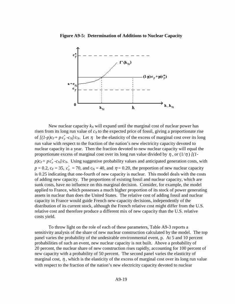
A9-19

Figure A9-5: Determination of Additions to Nuclear Capacity

New nuclear capacity kN will expand until the marginal cost of nuclear power hasrisen from its long run value of cN to the expected price of fossil, giving a proportionate riseof [(1-p)cF+ p *

Fc -cN]/cN. Let η be the elasticity of the excess of marginal cost over its longrun value with respect to the fraction of the nation’s new electricity capacity devoted tonuclear capacity in a year. Then the fraction devoted to new nuclear capacity will equal theproportionate excess of marginal cost over its long run value divided by η , or (1/η ) [(1-

p)cF+ p *Fc -cN]/cN. Using suggestive probability values and anticipated generation costs, with

p = 0.2, cF = 35, *Fc = 70, and cN = 40, and η = 0.20, the proportion of new nuclear capacity

is 0.25 indicating that one-fourth of new capacity is nuclear. This model deals with the costsof adding new capacity. The proportions of existing fossil and nuclear capacity, which aresunk costs, have no influence on this marginal decision. Consider, for example, the modelapplied to France, which possesses a much higher proportion of its stock of power generatingassets in nuclear than does the United States. The relative cost of adding fossil and nuclearcapacity in France would guide French new-capacity decisions, independently of thedistribution of its current stock, although the French relative cost might differ from the U.S.relative cost and therefore produce a different mix of new capacity than the U.S. relativecosts yield.

To throw light on the role of each of these parameters, Table A9-3 reports asensitivity analysis of the share of new nuclear construction calculated by the model. The toppanel varies the probability of the undesirable environmental event, p. At 5 and 10 percentprobabilities of such an event, new nuclear capacity is not built. Above a probability of20 percent, the nuclear share of new construction rises rapidly, accounting for 100 percent ofnew capacity with a probability of 50 percent. The second panel varies the elasticity ofmarginal cost, η , which is the elasticity of the excess of marginal cost over its long run valuewith respect to the fraction of the nation’s new electricity capacity devoted to nuclear

A9-20

capacity. When that elasticity takes a very low value, nuclear construction costs rise verylittle when rapid construction occurs, and it is reasonable that under such circumstances thenuclear share of new construction is very high. If the elasticity has a value of 1, the nuclearshare of new construction falls to 5 percent. In the third panel the nuclear cost is varied froma low value of parity with current fossil costs, $35 per MWh, to a high of $80 per MWh.When nuclear power costs are the same as current fossil costs, 100 percent of newconstruction is nuclear. However, the nuclear share drops off rapidly as the nuclear cost risesabove $40 per MWh. Between $40 and $50 per MWh, the nuclear share of new constructionfalls to zero. The bottom panel varies the future fossil cost. A high future fossil cost isimportant to the nuclear share of new construction. Between fossil costs $60 and $70 perMWh, the nuclear share begins to rise to 25 percent at the base-case value of $70 per MWhand to 50 percent at $80 per MWh.

Given the importance of the topic, it would be highly desirable to undertake futureresearch on refining estimation of the p’s, c’s, and the )(’ Nkf function. The latter would

entail investigating the lags encountered in adjusting human capital and applied R&D whennuclear capacity expands and analyzing rising costs encountered in the expansion.

A9-21

Table A9-3: Sensitivity of Model Calculation of Nuclear Share of New Construction

Vary p (probability of environmental costs)Parameter values

ParametersBase case

p probability of environmental costs 0.05 0.1 0.2 0.3 0.5 elasticity of marginal cost 0.2 0.2 0.2 0.2 0.2

c1 current fossil cost ($ per MWh) 35 35 35 35 35c2 current nuclear cost ($ per MWh) 40 40 40 40 40c3 future fossil cost ($ per MWh) 70 70 70 70 70Nuclear share of new construction 0 0 0.25 0.69 1.00

Vary (elasticity of marginal cost)Parameter values

ParametersBase case

p probability of environmental costs 0.2 0.2 0.2 0.2 0.2 elasticity of marginal cost 0.05 0.1 0.2 0.5 1

C1 current fossil cost ($ per MWh) 35 35 35 35 35C2 current nuclear cost ($ per MWh) 40 40 40 40 40C3 future fossil cost ($ per MWh) 70 70 70 70 70Nuclear share of new construction 1 0.5 0.25 0.1 0.05

Vary cN (nuclear cost)Parameter values

Parameters Basecase

p probability of environmental costs 0.2 0.2 0.2 0.2 0.2 elasticity of marginal cost 0.2 0.2 0.2 0.2 0.2

C1 current fossil cost ($ per MWh) 35 35 35 35 35C2 current nuclear cost ($ per MWh) 35 40 50 60 70C3 future fossil cost ($ per MWh) 70 70 70 70 70Nuclear share of new construction 1 0.25 0 0 0

Vary *Fc (future fossil cost)

Parameter valuesParameters Base

casep probability of environmental costs 0.2 0.2 0.2 0.2 0.2

elasticity of marginal cost 0.2 0.2 0.2 0.2 0.2C1 current fossil cost ($ per MWh) 35 35 35 35 35C2 current nuclear cost ($ per MWh) 40 40 40 40 40C3 future fossil cost ($ per MWh) 50 60 70 75 80Nuclear share of new construction 0 0 0.25 0.38 0.5

A9-22

A9.4.3. Appendix

Much additional work on energy portfolio considerations, beyond the scope of thepresent study, could be undertaken. The following preliminary discussion indicates possibledirections.

Consider a representative consumer, where each period is endowed with 1 unit of anon-storable resource (time for instance) that can be used solely to generate electricity. Theconsumer can choose between two generation technologies–nuclear and fossil fuel. Thereturn from the nuclear technology is risk-free, while the return from the fossil fueltechnology is not. In particular, suppose that each period there are two possible states of theworld–peace ( p ) with probability tπ and war ( w ) with probability1 tπ− . Then the return

on each technology (the amount of electricity generated using one unit of the resource withthe given technology) is given by

( ) ( )

n n

ff ff

tech \ state p w

N R R

FF R p R w

with ( ) ( )ff n ffR p R R w> > . For simplicity, assume that each of the two technologies islinear in the amount of the resource used. The generated electricity, e , can then be used toproduce consumption, c , using the technology

( ) 0 1c f e Aeα α= = , < < . (1)

The consumer’s preferences are represented by the utility function

11( ) 0

1U c c σ σ

σ−= , ≥

−(2)

with σ as the (constant) coefficient of relative risk aversion. We will analyze two differentcases, depending on different assumptions about the availability of the electricity generatingtechnologies and the timing of the decision which technology to use.

Consider the following three assumptions:

Assumption 1: Both generation technologies are freely available and there is no capacityconstraint–that is, all of the resource can be used with a given technology.

A9-23

Assumption 2: The consumer decides what fraction of the resource will be used with eachgeneration technology before the state of the world is known.

Assumption 3: There are no environmental externalities.

In this case, the consumer solves

)]),()1([(’0}{

max zRqRqfUE fft

ntt

t

t

qt

−+∑∞

=

β (3)

where { }z p w= , , tE is the conditional expectation operator, and tq is the fraction of the

resource that will be used with the nuclear technology in period t . Since there is nointertemporal decision in this case, the above problem is equivalent to

)])()1([(max}10{

zRqRqfUE fft

ntt

qt

−+≤≤

(4)

The first order condition for program (4) is

[ ( ( ))] [ ( )][ ( )]n fftU f e p f e p R R pπ ′ ′ − +

(1 ) [ ( ( ))] [ ( )][ ( )] 0n fft t tU f e w f e w R R wπ µ λ′ ′− − + − = (5)

where ( )e z is the amount of electricity generated in state z , tπ is the conditional probability

of peace, and tµ and tλ are Lagrange multipliers on the constraints 0tq ≥ and 1 0tq− ≥respectively. It thus follows that

(6)

as 1tq = and 0tq = respectively, while (4) holds with equality for any interior value of tq .

Evaluating expression (6) at equality and using the particular functional forms for ( )U . and( )f . we obtain

1 (1 )( ) [ ( ) ][ ] ( )

( ) 1 [ ( )]

ff nt

n fft

e p R p R

e w R R wα σ π

π− − −= .

− −(7)

)]([’))(([’

)]([’)](([’

pefpefU

wefwefU

)]([

])([

1 wRR

RpRffn

nff

i

i

−−

−ππ

A9-24

Let

1 [1 (1 )][ ( ) ]{( ) }

1 [ ( )]

ff nt

n fft

R p RB

R R wα σπ

π/ − −−≡ .

− −

Then (7) becomes

;)()1(

)()1(B

wRqqR

pRqqRffn

ffn

=−+−+

this in turn gives

( ) ( )

( ) ( ) (1 )

ff ff

ff ff n

BR w R pq

BR w R p B R

−= .− + −

(8)

Since ( ) ( ) (1 ) 0ff ff nBR w R p B R− + − < , the inequalities in (6) are reversed, giving tq q∗ as

1q ≥ and 0q ≤ respectively. The optimal fraction of the resource devoted to the nucleartechnology is therefore given by

{ {0 } 1}q Min Max q∗ = , , . (9)

For interior solutions we can calculate various elasticities of q∗ . In particular,

lnd q

dπε ππ

= (10)

with

ln ( ) ( ) ( )[ ( )]

( ) ( ) ( ) ( ) (1 )

ff n ff

ff ff ff ff n

d q dB d R w dB d R R w

d BR w R p BR w R p B R

π ππ

/ / −= +− − + −

and

[1 (1 )] (1 )

dB B

dπ α σ π π= .

− − −

A9-25

Similarly,lnd q

dσε σσ

= (11)

where lnd q dσ/ has exactly the same form as lnd q dπ/ with dB dσ/ in place of dB dπ/ ,while

2

[ ( ) ]ln{( ) }

[1 (1 )] 1 [ ( )]

ff nt

n fft

dB B R p R

d R R w

α πσ α σ π

−= .− − − −

The principal factor involved in this characterization of the electricity portfolioproblem is adjustment costs: without higher costs from having to build new nuclear capacityrapidly should a particular state of the world occur, it would be sensible to wait for that stateof the world to emerge before building. However, with higher costs of rapid investment, itpays to have some of the nuclear asset in reserve. This is a form of insurance policy, inwhich possessing some amount of the more expensive asset lets producers avoid some costswith some probability.

Still another approach is that of real options, or irreversible investment theory(Pindyck 1991, Dixit and Pindyck 1994). The value of current investments in energy R&Dhas been studied with real options models (Schimmelpfennig 1995, Davis and Owens 2003).Guillerminet (2001) has used an options model to study investment in nuclear power as ahedge against the possibility that the cost of fossil generation will rise.

A9-26

References

Abraham, Spencer. (2004). Luncheon Address to the Keidanren, Tokyo, Japan. January 9.

Bush, George W. (2004) Statement to students at Niles High School. Niles, Mich., May 24.Retrieved from Worldwide Web May 2004: http://www.nei.org/doc.asp?docid=1196.

Davis, G., and B. Owens. (2003) “Optimizing the Level of Renewable Electric R&DExpenditures Using Real Options Analysis.” NREL/TP-620-31221. Golden, Colorado:National Renewable Energy Laboratory, February.

Dixit, Avinash K., and Robert S. Pindyck. (1994) Investment Under Uncertainty.Princeton: Princeton University Press.

Energy Information Administration (EIA). (2003a) Annual Energy Outlook 2003.Washington, D.C.: U.S. Department of Energy.

Energy Information Administration (EIA). (2003b) Retrieved September 10, 2003 from theWorld Wide Web: www.eia.doe.gov/emeu/international/ngasprie.html.

Energy Information Administration (EIA). (2003c) Retrieved September 10, 2003 from theWorld Wide Web: www.eia.doe.gov/emeu/international/ngasprii.html.

Energy Information Administration (EIA). (2003d) Retrieved September 10, 2003 from theWorld Wide Web: www.eia.doe.gov/emeu/international/ngasprih.html.

Energy Information Administration (EIA). (2004) Annual Energy Outlook 2004 withProjection to 2025. Washington D.C.: Energy Information Administration, January.Supplemental tables retrieved from the World Wide Web January 2004:http://www.eia.doe.gov/oiaf/aoe/excel/aeo_base.xlsEnergy Research Board (ERB). (2001) “Canadian Natural Gas: Market Review andOutlook.” Canada. Retrieved January 7, 2004 from the World Wide Web:http://www2.nrcan.gc.ca/es/erb/prb/english/View.asp?x=447&oid=651.

Fisher, William L. (1994) “How Technology Has Confounded U.S. Gas ResourceEstimators,” Oil & Gas Journal 92, October 24: 100-107.

Greenspan, Alan. (2003) “Natural Gas Supply.” Testimony before Senate Committee onEnergy and Natural Resources, Federal Reserve Board.

Guillerminet, Maire-Laure. (2001) “La décision d’investissement en électricité et sonfinancement dans un environmennement institutionnel en mutation.” Mimeo. Paperpresented at Colloque international “La nécessité de nouvelles régulations internationalesface aux mutations énergétiques et environmennementales,” Paris, June 10-13. Downloadedfrom Worldwide Web December 2003: http://www.sceco.univ-montp1.fr/creden/Reseau/DOCS%20COLLOQUE/M_L_Guillerminet. pdf.

A9-27

Hamilton, James D. (1983) “Oil and the Macroeconomy since World War II,” Journal ofPolitical Economy 91: 228-248.

Jensen, James T. (2003) “The LNG Revolution,” The Energy Journal 24, No. 2: 1-45.

Jones, Donald W., Inja K. Paik, and Paul N. Leiby. (2004) “Oil Price Shocks and theMacroeconomy: What Has Been Learned Since 1996,” forthcoming in The Energy Journal25, No. 2: 1-32.

National Energy Policy Development Group (NEPDG). (2001) National Energy Policy:Reliable, Affordable, and Environmentally Sound Energy for America’s Future. Report ofthe National Energy Policy Development Group. Washington, D.C.: U.S. GovernmentPrinting Office, May.

National Petroleum Council (NPC). (1999) “Meeting the Challenges of the Nation’sGrowing Natural Gas Demands.” Washington, D.C., December 1999.

National Petroleum Council (NPC). (2003) “Balancing Natural Gas Policy – Fueling theDemands of a Growing Economy.” Washington, D.C., September 2003.

Pindyck, Robert S. (1991) “Irreversibility, Uncertainty, and Investment,” Journal ofEconomic Literature 29: 1110-1148.

Schimmelpfennig, D. (1995) “The Option Value of Renewable Energy: The Case ofClimate Change,” Energy Economics 17: 311-317.

Schmoker, James W., and Thaddeus S. Dyman. (2001) Changing Perceptions of UnitedStates Natural Gas Resources as Shown by Successive U.S. Department of the InteriorAssessments. U.S. Geological Survey Bulletin 2172-B. Washington, D.C.: U.S. GeologicalSurvey.

Simmons, M.R. (2003) “Future Energy Resources: Are We Asking the Right Questions.”National Defense University Workshop, Simmons International.

Smith, R., and A. Hove. (2003) “Utilities: The Old Reliables.” Deutsche Bank AG.

Stokey, Nancy L., and Robert E. Lucas, Jr., with Edward C. Prescott. (1989) RecursiveMethods in Economic Dynamics. Cambridge, Mass.: Harvard University Press.

U.S. Department of Energy (DOE) and Nuclear Power Industry. (2004). Strategic Plan forLight Water Reactor Research and Development. First Edition. Washington, D.C.: Officeof Nuclear Energy, Science and Technology; Nuclear Energy Institute, and Electric PowerResearch Institute, February.

A9-28

Webber, Jude. (2003) “Bolivia May Miss the Boat on Natural Gas Exports,” Reuters,October 20. Retrieved December 2003 from the World Wide Web:http://www.latinpetroleum.com/article_2295.shtml

ACM-1

ACRONYMS

Acronym DefinitionABB-CE Asea Brown Boveri - Combusion EngineeringABI Allied Business IntelligenceABWR Advanced Boiling Water ReactorACR Advanced CANDU ReactorACRS Accelerated Cost Recovery SystemAEA Atomic Energy ActAEC Atomic Energy CommissionAECL Atomic Energy Canada, LimitedAEO Annual Energy OutlookAFR Advanced Fast ReactorAFP Agence France PresseAFUDC Allowance for funds used during constructionAGR Advanced Gas Cooled ReactorAHTR Advanced High Temperature ReactorALWR Advanced Light Water ReactorAMIGA All Modular Industry Growth Assessment Modeling SystemANL Argonne National LaboratoryANP Advanced Nuclear PowerAPWR Advanced Pressurized Water ReactorASM Annual Survey of ManufacturesBALANCE Energy network module from ENPEPBBC British Broadcasting CorporationBBL. BarrelsBEA Bureau of Economic AnalysisBGS British Geological SurveyBLS Bureau of Labor StatisticsB/M Book to marketBNFL British Nuclear Fuels, Ltd.BOE Barrel of oil equivalentBtu British thermal unitBW Business WeekBWR Boiling Water ReactorCAAA Clean Air Act AmendmentsCANDU Canada Deuterium UraniumCAPM Capital asset pricing modelCCAPM Consumption-based capital asset pricing modelCCGT Combined cycle gas turbineCF Capacity factorCFB Circulating fluidized bedCFR Code of Federal Regulations

ACM-2

Acronym DefinitionCHP Combined Heat-and-PowerCIF Cost, insurance, and freight charges for shipping productsCM Census of Manufactures CO2 Carbon dioxideCOGEMA COGEMA Nuclear FuelsCOL Construction and Operating LicenseCNN Cable News NetworkCPI-U Urban Consumer Price IndexCPS Coal Production SubmoduleCPS Current Population SurveyCRDM Control rod drive mechanismCTBT Comprehensive Test Ban TreatyD&D Decommissioning and decontaminationDIGEC Direction du gaz, de l’ électricité et du charbonDoD Department of DefenseDOE U.S. Department of EnergyDOJ Department of JusticeEAR Estimated additional resourcesECAR East Central Area ReliabilityECP Electricity Capacity and PlanningEdF �lectricité de FranceEERE Energy Efficiency and Renewable EnergyEFP Electricity Financing and PricingEGRID Emissions & Generation Resource Integrated Database, U.S.EPAEIA Energy Information AdministrationEIS Environmental Impact StatementEMM Electricity Market ModuleENEA European Nuclear Energy AgencyENPEP Energy and Power Evaluation ProgramEPA U.S. Environmental Protection AgencyEPC Engineer-procure-constructEPR European Pressurized ReactorEPRI Electric Power Research InstituteERB Energy Research BoardERCOT Electric Reliability Council of TexasESBWR European Simplified Boiling Water Reactor ESP Early Site PermitEURATOM European Atomic Energy CommunityEV Electric vehicleEVA Energy Ventures Analysis, Inc.F-ANP Framatome Advanced Nuclear PowerFBC Fluidized bed combustionFBR Fast Breeder Reactor

ACM-3

Acronym DefinitionFCHV Fuel cell hybrid vehicleFCV Fuel cell vehicleFCX Honda FCX fuel cell vehicleFEMA Federal Emergency Management AgencyFERC Federal Energy Regulatory CommissionFOAKE First-of-a-kind-engineeringFOB Free on board, shipper pays shipping costsFRCC Florida Reliability Coordinating CouncilGA General AtomicsGCR Gas Cooled ReactorGDP Gross Domestic ProductGE General ElectricGenSim Electricity Generation Cost Simulation ModelGHG Greenhouse gasGII Global Insights, Inc.GM General MotorsGt GigatonnesGTCC Gas Turbine Combined CycleGT-MHR Gas-Turbine Modular Helium ReactorGW GigawattHg MercuryHLW High-level wasteHTGR High-Temperature Gas-Cooled ReactorHRSG Heat recovery steam generationHWLWR Heavy-Water-Moderated, Light-Water-CooledIAEA International Atomic Energy AgencyICE Internal combustion engineIDC Interest during constructionIIASA International Institute for Applied Systems AnalysisIEA International Energy AgencyIGCC Integrated gasification combined cycleILW Intermediate level wasteIPM Integrated Planning ModelIPP Independent Power PlantIRIS International Reactor Innovative and SecureIRR Internal rate of returnITS Institute of Transportation StudiesJAERI Japan Atomic Energy Research Institutekg KilogramkgHM Kilograms of heavy metalKgU Kilogram of uraniumkW KilowattkWh Kilowatt hour

ACM-4

Acronym DefinitionLANL Los Alamos National LaboratoryLCOE Levelized cost of electricityLFEE MIT Laboratory for Energy and the Environmentln Natural logarithmLHV Lower heating valueLLW Low level wasteLNB Low-NOX burnerLNG Liquefied natural gasLWGR Light Water Cooled Graphite ReactorLWR Light-water reactorMAAC Mid-Atlantic Area CouncilMACRS Modified Accelerated Cost Recovery SystemMAIN Mid-America Interconnected NetworkMAPP Mid-Continent Area Power PoolMEA MonoethanolamineMESSAGE Model for Energy Supply Strategy Alternatives and their General

Environmental ImpactMHR Modular helium reactorMIT Massachusetts Institute of TechnologyMITI Ministry of International Trade and IndustryMMBtu Thousand Thousand British Thermal UnitsMOX Mixed-oxideMSLL Materials System LaboratoryMT Metric tonMtoe Millions of tons of oil equivalentMtu Metric ton of uraniumMW MegawattMWh Megawatt hourNAC Nuclear Assurance CorporationNEA Nuclear Energy AgencyNEEDS National Electric Energy Database SystemNEI Nuclear Energy InstituteNEMS National Energy Modeling SystemNEPA National Environmental Policy ActNEPDG National Energy Policy Development GroupNEPOOL New England Power PoolNERC North American Electric Reliability CouncilNERI Nuclear Energy Research InitiativeNPC National Petroleum CouncilNPT Nuclear Non-Proliferation TreatyNOX Nitrogen oxideNPC National Petroleum CouncilNRC National Research Council

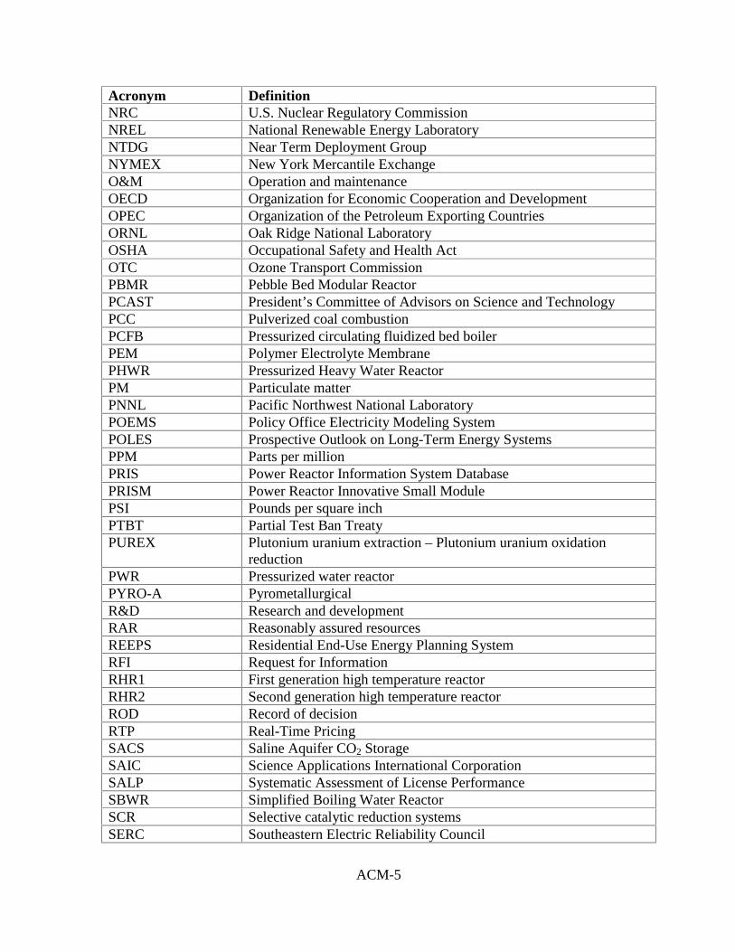
ACM-5

Acronym DefinitionNRC U.S. Nuclear Regulatory CommissionNREL National Renewable Energy LaboratoryNTDG Near Term Deployment GroupNYMEX New York Mercantile ExchangeO&M Operation and maintenanceOECD Organization for Economic Cooperation and DevelopmentOPEC Organization of the Petroleum Exporting CountriesORNL Oak Ridge National LaboratoryOSHA Occupational Safety and Health ActOTC Ozone Transport CommissionPBMR Pebble Bed Modular ReactorPCAST President’s Committee of Advisors on Science and TechnologyPCC Pulverized coal combustionPCFB Pressurized circulating fluidized bed boilerPEM Polymer Electrolyte MembranePHWR Pressurized Heavy Water ReactorPM Particulate matterPNNL Pacific Northwest National LaboratoryPOEMS Policy Office Electricity Modeling SystemPOLES Prospective Outlook on Long-Term Energy SystemsPPM Parts per millionPRIS Power Reactor Information System DatabasePRISM Power Reactor Innovative Small ModulePSI Pounds per square inchPTBT Partial Test Ban TreatyPUREX Plutonium uranium extraction – Plutonium uranium oxidation

reductionPWR Pressurized water reactorPYRO-A PyrometallurgicalR&D Research and developmentRAR Reasonably assured resourcesREEPS Residential End-Use Energy Planning SystemRFI Request for InformationRHR1 First generation high temperature reactorRHR2 Second generation high temperature reactorROD Record of decisionRTP Real-Time PricingSACS Saline Aquifer CO2 StorageSAIC Science Applications International CorporationSALP Systematic Assessment of License PerformanceSBWR Simplified Boiling Water ReactorSCR Selective catalytic reduction systemsSERC Southeastern Electric Reliability Council

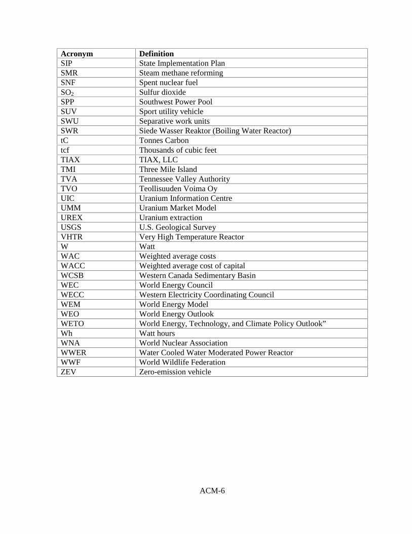
ACM-6

Acronym DefinitionSIP State Implementation PlanSMR Steam methane reformingSNF Spent nuclear fuelSO2 Sulfur dioxideSPP Southwest Power PoolSUV Sport utility vehicleSWU Separative work unitsSWR Siede Wasser Reaktor (Boiling Water Reactor)tC Tonnes Carbontcf Thousands of cubic feetTIAX TIAX, LLCTMI Three Mile IslandTVA Tennessee Valley AuthorityTVO Teollisuuden Voima OyUIC Uranium Information CentreUMM Uranium Market ModelUREX Uranium extractionUSGS U.S. Geological SurveyVHTR Very High Temperature ReactorW WattWAC Weighted average costsWACC Weighted average cost of capitalWCSB Western Canada Sedimentary BasinWEC World Energy CouncilWECC Western Electricity Coordinating CouncilWEM World Energy ModelWEO World Energy OutlookWETO World Energy, Technology, and Climate Policy Outlook”Wh Watt hoursWNA World Nuclear AssociationWWER Water Cooled Water Moderated Power ReactorWWF World Wildlife FederationZEV Zero-emission vehicle