The Earned Income Tax Credit and Food Consumption Patterns;

Fe

dera

l Res

erve

Ban

k of

Chi

cago

The Earned Income Tax Credit and Food Consumption Patterns Leslie McGranahan and Diane W. Schanzenbach

November 2013

WP 2013-14

1

The Earned Income Tax Credit and Food Consumption Patterns

November 20, 2013

Leslie McGranahan Diane W. Schanzenbach

Federal Reserve Bank of Northwestern University

Chicago and NBER

Abstract

The Earned Income Tax Credit is unique among social programs in that benefits are not paid out evenly across the calendar year. We exploit this feature of the EITC to investigate how the credit influences the food expenditure patterns of eligible households. We find that eligible households spend relatively more on healthy items including fresh fruit and vegetables, meat and poultry, and dairy products during the months when most refunds are paid.

JEL Codes: H3 (Fiscal Policies and Behavior of Economic Agents), I38 (Government Policy; Provision and Effects of Welfare Programs), Q18 (Agricultural Policy; Food Policy)

Keywords: Earned Income Tax Credit, Obesity, Healthy Eating, Food Expenditures

The opinions expressed in this paper are those of the authors and do not reflect the opinions of the Federal Reserve Bank of Chicago or the Federal Reserve System.

2

1. Introduction

The Earned Income Tax Credit (EITC) began in 1975 as a small program designed to offset payroll

taxes among low income working families with children. Over the subsequent four decades it has grown

into one of the largest means tested Federal programs. For Tax Year 2011, the Federal government

spent $63 Billion on the EITC rendering it the largest Federal cash assistance program and the second

largest non-health means tested program, after the Supplemental Nutrition Assistance Program (SNAP)

(IRS, 2013; CBO, 2013). The growth of the EITC has been the result of numerous policy expansions

which have both broadened the coverage of the program and dramatically increased benefit levels

among recipient families.

The EITC is structured as a subsidy to work among targeted families. Households receive a

benefit that equals a percentage of earnings up to a maximum credit amount. Households with earnings

along a plateau range also receive this maximum credit. Higher income households gradually see their

credit phase-out as earnings increase until the entire credit is phased out. This complex structure has

led researchers to investigate the labor supply effects of the EITC. Most academic research on the EITC

has highlighted the EITCs positive labor supply effects especially among single mothers. The EITC has

served to increase work participation among targeted households without reducing the labor supply of

working households. (For a summary see Hoynes and Eissa 2006).

A smaller body of research has investigated the effects of the EITC on household consumption

patterns. This research has highlighted the increase in work related expenditures among recipient

households (Patel 2011); a result consistent with the program’s large labor supply effects. Other

research has exploited the lump-sum nature of payments to investigate changes in spending around the

timing of benefit receipt (Barrow and McGranahan 2000; Goodman-Bacon and McGranahan 2008).

Most EITC recipients have received their benefits in the form of a lump sum payment that is part of the

household’s tax refund. Recipients had been permitted to receive some benefit payments in the

calendar year prior to tax filing via Advance EITC payments. However, due to minimal take-up of these

payments, the Advance EITC was repealed and no longer available after 2010. Previous research

focused on the timing of EITC receipt has found increases in spending on durables, especially cars, in

response to the large lump sum transfer. We exploit the lump-sum nature of EITC payments to

investigate how food spending among EITC recipients changes in the period of EITC receipt. In

particular, we investigate spending patterns in those months when most EITC benefits are received.

3

The focus of the paper is spending on food. We are interested in both overall food spending and

on its composition across food categories. According to the National Health and Nutrition Expenditure

Survey (NHANES), obesity is higher among the groups targeted by the EITC than other groups. In

particular, women with incomes below 130% of the poverty line have obesity rates 13 percentage points

higher than women with incomes above 350% of the poverty line (Ogden et al 2010A) while lower

income boys have obesity rates that are 10 percentage points higher and lower income girls have

obesity rates that are 7 percentage points higher (Ogden et al 2010B). Our analysis is informative about

the link between income and food consumption patterns. We are able to ask whether there are

changes in the spending patterns of EITC households during a period of the year when their income is

likely to be the highest.

Because of the link between socioeconomic status and obesity, a number of policy interventions

have sought to influence the food choices of low-income households. In particular, interventions have

sought to decrease the relative price and increase the availability of healthy foods. A growing body of

work has analyzed these interventions. One recent intervention, the Healthy Incentives Pilot (HIP), was

found to increase spending on fruits and vegetables among families that received a SNAP bonus for

money spent on fruits and vegetables (Bartlett et al. 2013). Our results are consistent with this finding

in that we observe that households make healthier food choices when they have more income.

In the current paper we use data from the Consumer Expenditure Diary Survey (Diary) to ask

how household food expenditure pattern change in the months when EITC benefits are received. In the

future, we hope to expand our analysis to include data from the NHANES and investigate food

consumption. We find that households receiving EITC benefits spend more on healthy foods and

protein in EITC months. We interpret these finds as telling us both how individuals spend their EITC

refunds and how low income household food choices respond to an increase in income.

Background on the EITC and Benefit Timing

As noted earlier, the generosity of the EITC has evolved over time. However, its basic structure

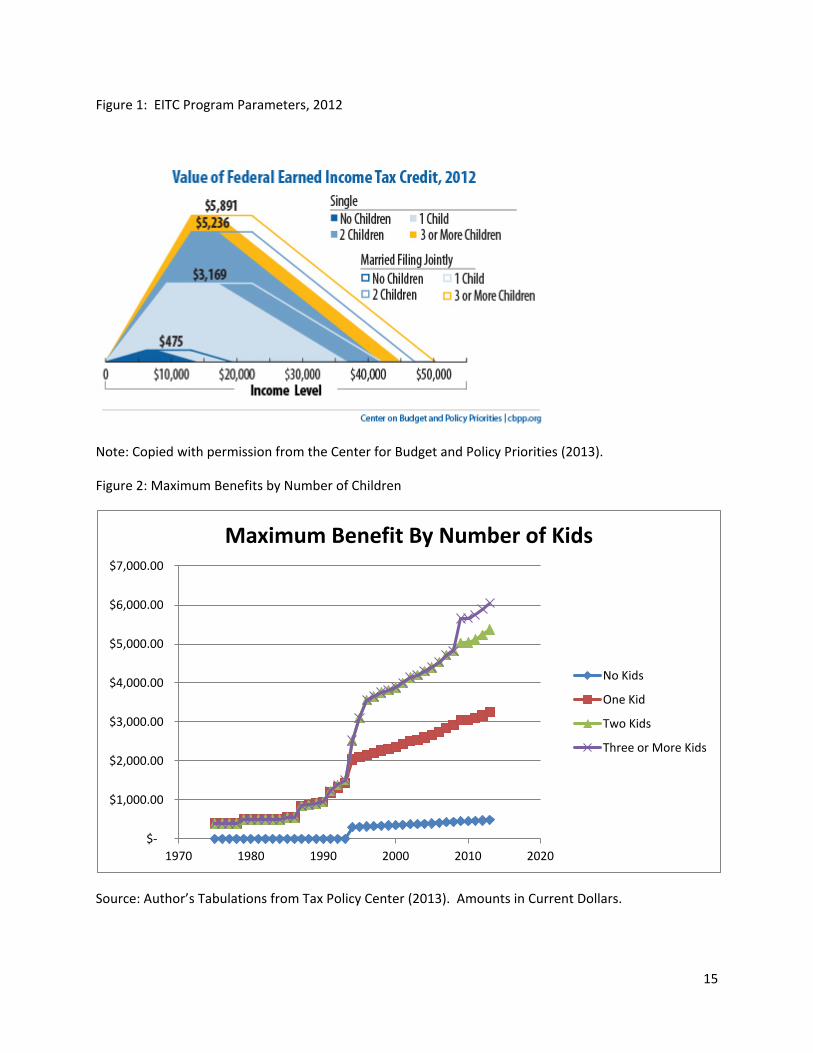
has remained unchanged with an earning subsidy, a plateau range, and a phase out range. In Figure 1,

we display a graph of the program parameters (as constructed by the Center for Budget and Policy

Priorities 2013) for 2012. As is shown in the Figure, there is a small benefit for childless households and

benefit schedules that increase in generosity for families with more children. In Figure 2, we graph the

(nominal) level of maximum benefits over time by family size. Through 1990, families with children

faced the same schedule independent of their size. From 1991 on, families with two or more children

4

received a higher benefit. Starting in 2009, families with three or more children received even higher

benefits. A small benefit for households without children was added in 1994.

The growing generosity of the program led to growing costs. Figure 3 graphs spending on all

Federal means tested programs (CBO 2013). Tax Credits (including the EITC and the much smaller Child

Tax Credit) have grown from a small portion of the safety net, to a major component of it.

Throughout its history, the EITC has been a refundable tax credit that has been part of the tax

code. It has been paid out along with filers’ tax refunds and has been fully refundable – credits in excess

of tax liability are paid out as refunds. Through 2010, filers could receive some EITC dollars in the form

of the Advance EITC, but this program was discontinued because it was characterized by high errors and

minimal take up.

Individuals who are expecting a fixed nominal benefit from the government have an incentive to

file their taxes and receive their refunds as early as possible. While many high income people wait until

the tax filing deadline on April 15th to file their taxes, EITC recipients tend to file early. In order to file

taxes an individual needs to have his W2 form and the IRS filing window needs to be open. Employers

are required by the Federal government to issue W-2s by January 31 and the tax window opens in mid-

January. In 2011, the window opened on January 14.1 The 2012 window opened on January 17 and in

2013 it opened on January 30. The day the window opens tends to be the first day that volunteer sites

open and is the first date that paid preparers can submit returns.2

Once the return is submitted, the IRS processes it and sends out refunds. According to the IRS,

under normal processing, refunds for e-filed returns are direct deposited two Fridays after the return is

filed and paper checks are mailed three Fridays after filing. Refunds from paper returns take longer –

approximately six to eight weeks. In 2010, sixty-nine percent of returns were filed electronically and

sixty-eight percent of refunds were direct deposited. These percentages have been increasing over time

and as a result payments have been being received progressively earlier.

In Figure 4, we display the percent of EITC refunds paid out by the IRS by month from selected

years in our sample period, 1982, 1992, 2002 and 2012 based on data from the US Treasury’s Monthly

1 In 2011, individuals with itemized deductions and some others needed to wait until mid-February to file 2010 taxes. This was due to late in year tax changes to extend the Bush tax cuts. 2 This is also the first day that Refund Anticipation Loans could be issued because they were issued when returns were filed.

5

Treasury Statement (MTS). These are refunds in excess of tax liability. Over 90% of the value of the EITC

is delivered in the form of tax refunds, as opposed to serving to reduce tax liabilities. Over this 20 year

time period, the pattern of EITC refunds has been fairly consistent. Payments have been sent out at the

beginning of the year. In the earliest years of the sample, the modal month was March, with large

payments in April and May and a smaller amount in February. In most recent years, the majority of

benefits have been paid by the IRS in February, another sizeable amount in March, modest amounts in

January and April and very few the remainder of the year.3 In Figure 5, we display the average month of

payments over the entire sample period (1982-2012). This demonstrates both that payments have been

getting earlier and that they occur very early in the year. In Figure 6, we compare the monthly pattern

for EITC refunds for 2012 to the pattern for overpayment refunds and the benefits of other income

support programs. The patterns for these other programs are quite different from the pattern for the

EITC. Temporary Assistance to Needy Families (TANF) and SNAP benefit payments are nearly constant

across the months of the year. Overpayment refunds are sent out in February, March and April with a

sizeable amount in May as well. Child Nutrition payments drop during the summer months but are fairly

constant during the school year.

The lump sum EITC payment is large when taken in the context of the incomes of targeted

households. The IRS reports that 28 million people filed EITC returns for tax year 2011 (refunds received

in early 2012 (IRS 2013). The average refundable credit was $1,983. The average ranged from $188 for

families with no kids to $3,342 for families with three kids or more. These amounts represent 3% of the

AGI of the average recipient household without kids of $6,763 and 14% of the average AGI of a recipient

family of $24,198 with three kids or more (IRS 2013). If we assume that a household receives an amount

equal to 1/12th of its AGI in the month it receives the EITC, in that month, the income of the average

household increased by 39% for the household without kids and by 163% for the households with three

kids. These increases are even more dramatic in the more generous ranges of the EITC. A household

with three kids earning $12,780 a year would receive an EITC of $5,751 which would increase its

monthly income five-fold. The EITC program pays out a substantial sum of money to a specific group of

households over a very narrow window of time.

2. Data

3 2004 is an exemption to this pattern. This difference from other years was only seen for EITC payments and not for other refunds. It may be due to some additional efforts to reduce EITC noncompliance.

6

We use data from the Diary portion of the Consumer Expenditure Survey (CEX) from 1982-2011

to investigate the expenditure response to the EITC. The unit of analysis in the CEX is the “Consumer

Unit (CU)” which is conceptually similar to a “household” and we use these terms interchangeably. The

data contain information on the weekly spending of household based on entries in spending diaries.

Households are asked to detail the food (and other) items they purchased independent of the means of

payment. Importantly for our analysis, items purchased with Food Stamps are treated the same as

items paid for in other ways.4 We do not have data on prices and quantities separately, but only on

expenditures. Each diary covers spending for one week. Households are in the sample for two

consecutive weeks. The Dairy is intended to cover spending on frequently purchased items such as

groceries. By comparison, the better known CEX Interview Survey focuses more on big ticket items. In

keeping with this distinction, in the creation of weights for the Consumer Price Index, the Bureau of

Labor Statistics uses the Diary data to measure consumption for nearly all food and beverage spending

categories. The microdata contain spending information on food at home and food away from home in

aggregate as well as for fairly detailed subcategories. For example, in addition to data on weekly

household spending on fresh fruit, we also have separate data on spending on apples, bananas, and

oranges.

The data also contain information on the socio-demographics of the household, measures of

household income, and limited data on social program receipt. There are a number of questions

concerning SNAP receipt, but there is no data on EITC receipt.

Following Barrow and McGranahan (2000), we combine individuals within the CU to create tax

units and impute EITC based on the earned income of the individuals in these tax units, tax unit

composition and the EITC schedule. The income data in the Diary is not tax year income, but rather

income in the twelve months leading up to the survey date. We assume that this income is equal to the

income in the previous tax year and impute EITC based on that. For example, a household with three

children observed in June 2004 that reports $20,000 of income is assumed to have made $20,000 in tax

year 2003 and been eligible for an EITC benefit of $2,884 based on the 2003 tax schedule. They are

imputed as EITC eligible in June 2004. Their refund would have been received when 2003 taxes were

filed in early 2004.

4 The instructions specifically say to include payments by “Food Stamps” and “WIC Voucher.” BLS 2013.

7

There is a change in the treatment of income during out sample period. In particular, income

imputation began in 2004. As a result, reasonable income values are provided for all households at this

point, not just those deemed to be complete income reporters. We restrict our sample to complete

income reporters prior to 2004, but include all households in later years. In Appendix A, we discuss how

well our EITC imputation procedure works by comparing data from our CEX based imputation to data

from the IRS.

In Table 1, we display variable means from our sample, both for the overall population and by

imputed EITC eligibility. Observations are at the Consumer Unit-by-week level, and we restrict the

sample to households headed by individuals aged 18-65. In the first panel of the Table, we display

means of weekly food spending. We break food into food at home and food away from home and

further divide these into a series of categories. We also add three special categories at the bottom of

the table that may be of interest to policy makers – sugar sweetened beverages, junk food and healthy

food. The contents of these categories are displayed in Table 2. The average consumer unit spends

$130 per week -- $80 of this on food consumed at home and $50 on food consumed away from home.

When we compare by imputed EITC eligibility, we note that EITC households spend less on average.

They spend a similar amount on food at home and a far lower amount on meals away from home – in

particular at full service restaurants.

Panel B of Table 1 shows means of the socio-demographic variables. EITC households are larger

on average, contain more children, are more likely to be less educated and female headed, and are far

lower income. All of these are consistent with a program that is designed to help low income families

with young children. In the sample, 15% of households are imputed to be EITC eligible. This ranges

from 7 percent in the early years of the sample and increases to over 20% in the most recent years. The

average EITC benefit is over $1500, or about 2.5 times average weekly income among recipients. By

comparison, the average recipient is imputed to receive about $70 from state EITC programs.5 Many

recipients also report receiving Food Stamps. However, other studies (see for example Meyer, Mok and

Sullivan 2008, and Hoynes, McGranahan and Schanzenbach 2013) indicate that Food Stamp receipt is

severely underreported in the CEX data.

3. Results and Methodology

5 We only impute state EITC receipt for those individuals where the state code is not suppressed in the microdata.

8

To investigate the impact of the EITC on food spending, we begin by estimating the

determinants of food spending in general. We estimate:

it i i t t itE X EITC M Yα β γ ε= + + + + + (Equation 1)

Where itE is expenditure by CU i at time t. iX is a series of socio-demographic characteristics assumed

to affect food spending, iEITC is a dummy equal to 1 if the CU is imputed to be EITC eligible, tM is a

series of monthly dummies designed to capture the monthly seasonality in food consumption and prices

which is assumed to be constant across years. For example, this will capture high candy spending in

October. tY is a series of year dummies which capture changing aggregate prices, consumer preferences

and survey categorization. itε is an error term.

The results for estimating equation 1 via OLS for seventeen different categories of food

spending are presented in Table 3. Each column in the table displays the result for a different

regression. Spending on all seventeen categories is increasing in family size and income. Spending is

lower for families with more children in most categories in keeping with their lower caloric needs. The

exceptions to this pattern are cereal and bakery products, dairy products, sweets and junk food. We

also find that spending is higher across all categories in the first interview. This is likely a sign of

interview fatigue where the respondent enthusiasm wanes in the second diary week. Male headed

households spend less on food at home and more on food away from home. Households imputed to be

EITC eligible generally consume less across most categories even controlling for these other covariates.

Having established overall expenditure patterns, we now turn to whether these expenditure

patterns change differentially among EITC households in those months when households are likely to

receive their EITC. We first do this by adding to Equation 1 a series of interactions between the iEITC

dummy and the month dummies. In particular, we estimate

it i i i t t t itE X EITC EITC M M Yα β γ λ ε= + + + × + + + (Equation 2)

Where λ is a vector of month-specific expenditure responses for EITC eligible households. This tells us

whether the monthly spending pattern of EITC households differs from the pattern of other households.

We display coefficient estimates for the EITC dummy and the EITC month interactions in Table 4. We

omit the September interaction. As a result these effects are relative to spending among EITC

9

households in September. In the bottom two rows of the tables, we show the average of the February

and March coefficients and a test of whether these coefficients are jointly different from zero. We look

at these two months, because most benefits have been received in those months according to the MTS

data.6

For overall food spending (column 1), we find that food spending is relatively lower for EITC

households in most months than it is in September – most of the coefficients are negative. The two

largest coefficients are in February and March, but we can’t reject that the February and March marginal

EITC effects are equal to zero. The results differ across the different food categories. There are only five

food expenditure categories for which the results in February and March are jointly different from zero.

We observe significantly higher spending on meat, poultry, fish and eggs, dairy, fresh fruit and

vegetables, and healthy food. We see lower spending on processed fruit and vegetables.

There are a couple of limitations to this methodology. First, the fact that it compares spending

to September may or may not be appropriate. Additionally, it only looks at February and March and

treats them the same. However, in the early years of the EITC most benefits were paid out in March,

while in more recent years most benefits have been paid in February. We next propose a methodology

that addresses these issues. We calculate a variable share_EITC which measures the share of annual

EITC benefits paid out in a given month and year. For example, this variable would take on the value

0.59 in February 2006 because fifty-nine percent of 2006 benefits were paid out in February according

to the MTS. By contrast it takes on the value 0.17 in February 1982 because seventeen percent of 1982

benefits were paid out in February. We replace the month-EITC interaction with the measure of the

share of annual benefits paid out in a given month interacted with the EITC dummy. Our new equation

is:

_it i i t i t t itE X EITC share EITC EITC M Yα β γ χ ε= + + + × + + + (Equation 3)

The coefficient χ measures whether EITC eligible households spend relatively more in months when

more EITC is paid out – controlling for other covariates, the different demand of EITC households, yearly

6 Two factors push the benefits earlier than is captured by the MTS data. First the MTS data only measure the refundable portion. About 10% of EITC benefits are in the form of reduced tax liability. Presumably this type of benefit is received when taxes are filed. Second, recipients may expedite receipt of funds via Refund Anticipation Loans (RALs). These tend to be one to two week loans that allow recipients to receive funds when taxes are filed. According to Wu (2012) 18% of EITC recipients received RALs in 2010. RALs are no longer legal (as of April 2012). Their replacement, Refund Anticipation Checks (RACs), do not expedite fund availability.

10

trends and monthly seasonality. The results are presented in Table 5. The coefficient 12.64 in the

second row of column one can be interpreted that if 100% of EITC benefits were paid in a given month,

we would expect EITC households to spend an additional $12.64 on food in each week of that month.

We don’t see negative coefficients for any of the share-EITC interactions for any of the categories and

see statistically significant increases in food, food at home, meat, poultry, fish and eggs, dairy, fresh fruit

and vegetables, food away from home, fast food and healthy foods. In the bottom two rows of the

table, we add two calculated statistics. First, we calculate the percent increase in spending in each food

category by dividing the coefficient on the EITC-share interaction by average weekly food spending. A

$12.64 increase in spending would represent a 9.7% increase in average household spending on food.

The largest percentage increases are in meat, poultry, fish and eggs, dairy and healthy food. The

smallest increases are in fats and oils and sugar sweetened beverages. Second, in the final row of the

table we calculate the percent of average EITC benefits that would be spent on that food in a month

with a 100% share of EITC payments. To do this, we multiply the coefficient by 4.3 to translate the

weekly additional spending into monthly additional spending and divide this by the average imputed

benefit among those eligible. We find that about 3.5% of the average total benefit would be spent on

food.

Thus far in the analysis, we have not distinguished between different types of recipient

households such as those who are imputed to receive low benefit amounts and those imputed to

receive larger benefits. To some degree this is by design because the imputation procedure is bound to

be imprecise in the face of imperfect income data, and differences in the timing of reported income

(prior 12 months) and EITC period (prior calendar year). To investigate what role benefit amount and

other attributes play, we rerun the analysis for a series of population groups. We perform this analysis

for a subset of the 17 food spending categories. We choose to look at total food spending, food at

home, fresh fruits and vegetables, food away from home, healthy food and junk foods.

In Table 6, we display estimates of the coefficient on the interaction between the month EITC

share and the EITC dummy for different population subsets for the smaller set of spending categories.

Below each coefficient estimate we display the percentage increase in weekly spending in that food

category among that population would be estimated to occur if 100% of benefits were received in a

month and the additional percent of average EITC benefits among households in that subpopulation we

estimate would be spent on that category of food. In the first column, we repeat the results for the full

sample. In columns (2)-(4) we compare to other households that have characteristics typical of the

11

eligible. We find smaller and insignificant increases in total food spending among EITC households when

compared to other households with kids and households with a less educated head. We continue to

find large increases in healthy food spending for these two groups. When we compare EITC households

to other low income households, we continue to find increases in consumption across the same set of

expenditure categories that we did for the full sample. Our results also hold in columns (6)-(9) when we

drop those households from the analysis that we either impute to receive the small EITC for childless

families or are imputed to receive a small EITC. In columns (9) and (10) we divide the sample into first

and second interview households. Our results are much stronger for first interview households. We

find that total food spending increases by 16% and 6% of the average benefit was spent on food.

Looking across the food subcategories we find a 21% increase in healthy food spending and an 18%

increase in spending on fruits and vegetables in first interview weeks. We believe that the data

provided in the first interview is more accurate. In columns (11) and (12), we divide the sample into

male and female headed households. The results are broadly similar across the two household types.

Across all 12 specifications, we find increased spending on healthy foods. We find significant increases

in spending on junk foods in none of the specifications.

In Table 7, we show results dividing the households into three groups based on the year of the

diary. Our year groupings are designed to capture different periods in the life of the program. The first

period is 1982-1987 (tax years 1981-1986). We view this as part of the early low benefit period of the

program. During this period, the average imputed real benefit was $600. The second period is 1988-

1994 where benefits averaged $1089. We view this as the period of program expansion when the

benefits were increasing dramatically during many years. The final period is 1996 and after where

benefits averaged $1806. We view this as the stable high benefit period. For the early period, we see

no increases in food spending. In the second period, we see large increases in spending. Total food

spending is estimated to grow 16% in a month when 100% of benefits are paid. In the final period, we

see modest increases in spending. We see the largest increase in spending in the middle period when

benefits were growing the most rapidly, rather than in the last period when the benefits were the

highest. As a robustness check, we perform the same analysis for just the first household interview and

present the results in Table 8. We see a similar pattern with the largest spending increases in the middle

years. However, in this case we see increases in spending across all three time periods (although not

statistically significant in the earliest period). Some of the percentage increases in this case are quite

large with a 42% increase in spending on fresh produce between 1988 -1994 and increases in healthy

food spending ranging from 15% to 46%.

12

There are two potential explanations for observing the largest increases in the middle period.

First, this period is characterized by dramatic increases in benefits. This may mean that EITC households

were positively surprised when they found out their refund amount. Households may spend these

surprise benefits differently from anticipated benefits. As a second explanation, in the years after 1994,

the magnitude of the benefits may lead households to spend more of their money on big ticket items.

The large benefit checks may go directly to large durables rather than to food. We could partly clarify

these stories if we could look at spending responses in these different time periods in the interview data

where spending on large consumer durables is captured.

4. Conclusion

Using the Diary data from the Consumer Expenditure Survey, we have investigated whether

households imputed to be EITC eligible spend more on food and make different food choices in those

months when most EITC benefits are received.

We find that eligible households do spend more on food, and particularly on healthy foods in

those months when most benefits are paid. These effects are stronger in the first Diary interview when

data collection is likely to be more accurate (Cantor et al. 2013) and in the middle years of our sample.

Our results are robust across a number of subpopulations.

These findings are consistent with a growing literature that shows that low-income individuals make

better food choices when they are less constrained. Low income individuals eat healthier food when it

is more accessible. Recent interventions have shown that households purchase more healthy food when

it is more readily available or when it is relatively cheaper. We add to this discussion by finding that

they also purchase more healthy foods when they have more income. This finding also suggests that

decreases in resources, as occurred recently through the reduction in SNAP benefits, may have the

effect of reducing the diet quality of low income families.

13

References

Barrow, Lisa and Leslie McGranahan, 2000. “"The Effects of the Earned Income Credit on the Seasonality of Household Expenditures" National Tax Journal 53(4) (part 2): 1211-1244.

Bartlett et al. U.S. Department of Agriculture, Food and Nutrition Service, Office of Research and Analysis, “Healthy Incentives Pilot (HIP) Interim Report,” Project Officer: Danielle Berman, Alexandria, VA: July 2013.

Bureau of Labor Statistics (BLS). 2013. “Dairy Survey Form.”Available on the Internet at: http://www.bls.gov/cex/csx801_2013.pdf.

Bureau of Labor Statistics. Various Years. Consumer Expenditure Survey: Diary Survey.

Cantor, David, Nancy Mathiowetz, Sid Schneider and Brad Edwards. 2013 “Redesign Options for the Consumer Expenditure Survey,” Report prepared by Westat for the Bureau of Labor Statistics, June 21, 2013. Available on the Internet at http://www.bls.gov/cex/ce_gem_west_redesign.pdf.

Center for Budget and Policy Priorities, 2013, “Policy Basics: The Earned Income Tax Credit,” February 1, 2013. Available on the Internet at: http://www.cbpp.org/cms/?fa=view&id=2505

Congressional Budget Office, “Growth in Means-Tested Programs and Tax Credits for Low-Income Households.” February 11, 2013. Available on the web at http://www.cbo.gov/publication/43934.

Eissa, Nada & Hilary W. Hoynes, 2006. "Behavioral Responses to Taxes: Lessons from the EITC and Labor Supply," NBER Chapters, in: Tax Policy and the Economy, Volume 20, pages 73-110 National Bureau of Economic Research, Inc.

Goodman-Bacon, Andrew and Leslie McGranahan. 2008. “How Do EITC Recipients Spend their Refunds?” Economic Perspectives, Vol 32, 2nd Quarter.

Internal Revenue Service (IRS). 2011. “2011 IRS E-File Refund Cycle Chart” http://www.irs.gov/pub/irs-pdf/p2043.pdf.

Internal Revenue Service. 2013. SOI Tax Stats – Individual Income Tax Returns Publication 1304 (Complete Report), 2013. Available on the Internet at http://www.irs.gov/uac/SOI-Tax-Stats-Individual-Income-Tax-Returns-Publication-1304-(Complete-Report)

Internal Revenue Service. Various Years. Statistics of Income. Available on the Internet at http://www.irs.gov/uac/SOI-Tax-Stats-Archive---1954-to-1999-Individual-Income-Tax-Return-Reports.

Meyer, Bruce D, Wallace K.C. Mok and James X. Sullivan. 2009. “The Under-Reporting of Transfers in Household Surveys: Its Nature and Consequences.” NBER Working Papers 15181.

National Bureau of Economic Research. 2013. “State Earned Income Credits in TAXSIM.” Available on the Internet at http://users.nber.org/~taxsim/state-eitc.html.

http://www.bls.gov/cex/csx801_2013.pdf

http://www.bls.gov/cex/ce_gem_west_redesign.pdf

http://ideas.repec.org/h/nbr/nberch/0063.html

http://ideas.repec.org/h/nbr/nberch/0063.html

http://ideas.repec.org/s/nbr/nberch.html

http://www.irs.gov/pub/irs-pdf/p2043.pdf

http://www.irs.gov/pub/irs-pdf/p2043.pdf

http://www.irs.gov/uac/SOI-Tax-Stats-Individual-Income-Tax-Returns-Publication-1304-(Complete-Report)

http://www.irs.gov/uac/SOI-Tax-Stats-Individual-Income-Tax-Returns-Publication-1304-(Complete-Report)

14

Ogden Cynthia L, Lamb Molly M, Carroll Margaret D, Katherine M. Flegal. Obesity and socioeconomic status in adults: United States 2005–2008. NCHS data brief no 50. Hyattsville, MD: National Center for Health Statistics. 2010A. Available on the Internet at http://www.cdc.gov/nchs/data/databriefs/db50.pdf

Ogden, Cynthia L, Molly M. Lamb, Margaret D. Carroll Obesity and socioeconomic status in children and Adolescents: United States 1988–1994 and 2005–2008. NCHS data brief no 51. Hyattsville, MD: National Center for Health Statistics. 2010B. Available on the Internet at http://www.cdc.gov/nchs/data/databriefs/db51.pdf

Patel, Ankur. 2011. “The Earned Income Tax Credit and Expenditures,” mimeo University of California Davis.

Tax Policy Center, “Earned Income Tax Credit Parameters: 1975-2013,” January 28, 2013. Available on the Internet at: http://www.taxpolicycenter.org/taxfacts/Content/PDF/historical_eitc_parameters.pdf.

United States Department of the Treasury, Financial Management Service. Various Issues, “Monthly Treasury Statement.”

Wu, Chi Chi, “The Party’s Over for Quickie Tax Loans: But Traps Remain for Unwary Taxpayers,” February 2012. National Consumer Law Center and Consumer Federation of America. Available on the Internet at http://www.nclc.org/images/pdf/pr-reports/report-ral-2012.pdf

http://www.cdc.gov/nchs/data/databriefs/db50.pdf

http://www.taxpolicycenter.org/taxfacts/Content/PDF/historical_eitc_parameters.pdf

15

Figure 1: EITC Program Parameters, 2012

Note: Copied with permission from the Center for Budget and Policy Priorities (2013).

Figure 2: Maximum Benefits by Number of Children

Source: Author’s Tabulations from Tax Policy Center (2013). Amounts in Current Dollars.

$-

$1,000.00

$2,000.00

$3,000.00

$4,000.00

$5,000.00

$6,000.00

$7,000.00

1970 1980 1990 2000 2010 2020

Maximum Benefit By Number of Kids

No Kids

One Kid

Two Kids

Three or More Kids

16

Figure 3: Spending on Federal Means Tested Programs Time

Source: Congressional Budget Office, Growth in Means-Tested Programs and Tax Credits for Low-Income Households, February 11, 2013.

Figure 4: Monthly Shares of EITC Payments

Note: Authors’ tabulations from United States Department of the Treasury, Various Issues.

0

50

100

150

200

250

300

350

1972

19

75

1978

19

81

1984

19

87

1990

19

93

1996

19

99

2002

20

05

2008

20

11

Billi

ons o

f 201

2$

Year

Health

Tax Credits

Cash Assistance

Nutrition

Education (Pell)

Housing

0.2

.4.6

EIT

C R

efun

ds

1 2 3 4 5 6 7 8 9 10 11 12month

1982 1992 2002 2012

17

Figure 5: Average Month of Payment of EITC


Figure 6: Monthly Payment Shares, Selected Income Support Programs, 2012


2.5

33.

54

4.5

Ave

rage

Mon

th o

f EIT

C P

aym

ent

1980 1990 2000 2010 2020Year

0.2

.4.6

1 2 3 4 5 6 7 8 9 10 11 12month

EITC Refunds Overpayment Refunds

Supplemental Nutrition Assistance Program Benefits Federal TANF Payments

Federal Child Nutrition Spending

18

Table 1: Variable Means

Panel A: Food Expenditure Variables

MeanStandard Deviation Mean

Standard Deviation Mean

Standard Deviation

Food Total 129.98$ 118.90 132.22$ 120.52 117.38$ 108.38Food at Home 79.98$ 81.53 79.65$ 81.55 81.85$ 81.40Cereal & Bakery Products 11.54$ 14.38 11.50$ 14.47 11.74$ 13.86Meat Poultry Fish and Eggs 20.68$ 31.51 20.38$ 31.65 22.41$ 30.64Dairy 9.32$ 11.11 9.34$ 11.20 9.19$ 10.56Fresh Fruit and Veg 8.39$ 12.24 8.40$ 12.25 8.37$ 12.23Processed Fruit and Veg 5.03$ 7.67 5.02$ 7.67 5.08$ 7.68Sweets 3.06$ 6.77 3.08$ 6.88 2.92$ 6.08Non Alcoholic Bevs 7.32$ 10.49 7.30$ 10.58 7.40$ 9.98Oils 2.14$ 4.05 2.11$ 4.03 2.29$ 4.17Misc Food 12.52$ 18.11 12.53$ 18.11 12.45$ 18.13

Food Away 50.00$ 73.19 52.56$ 75.26 35.53$ 58.10Fast Food* 24.50$ 33.18 25.14$ 33.58 21.65$ 31.15Full Service* 24.51$ 50.91 26.89$ 53.25 13.88$ 36.97

Sugared Beverages 5.45$ 8.51 5.40$ 8.55 5.72$ 8.26Healthy Foods 28.21$ 31.04 28.01$ 30.90 29.31$ 31.83Junk Foods 9.85$ 13.93 9.94$ 14.12 9.35$ 12.80* Breakdown not available for all years of data** Average Weekly Spending, With Heads 18-65, 1982-2011, $2010

FULL SAMPLE NO EITC YES EITC

19

Panel B: Socio-Demographic Variables

Note: Authors’ tabulations from BLS, Various Years, deflated using BLS, Consumer Price Index, via Haver Analytics. Federal EITC parameters from Tax Policy Center, 2013. State EITC parameters from National Bureau of Economic Research, 2013.

MeanStandard Deviation Mean

Standard Deviation Mean

Standard Deviation

Family Size 2.73 1.54 2.58 1.47 3.62 1.65Persons Less Than 18 0.84 1.17 0.71 1.10 1.58 1.28Persons Over 65 0.04 0.22 0.05 0.23 0.03 0.19Age of Head 41.18 12.40 41.59 12.54 38.89 11.35Dummy=1 if Male Head 0.57 0.49 0.60 0.49 0.41 0.49Dummy=1 if Less Ed Head 0.41 0.49 0.38 0.49 0.59 0.49

Weekly Pre-Tax Income (1000s) 1.25$ 1.11 1.36$ 1.15 0.62$ 0.55Dummy=1 if First Interview 0.50 0.50 0.50 0.50 0.50 0.50Dummy=1 if Married 0.56 0.50 0.58 0.49 0.49 0.50

Dummy=1 if EITC 0.15 0.36 0.00 0.00 1.00 0.00Imputed EITC AMT 236.64$ 791.03 -$ 0.00 1,573.52$ 1434.29Imputed State EITC 13.19$ 106.50 -$ 0.00 68.62$ 223.69

Dummy=1 if SNAP Last Year 0.09 0.28 0.06 0.24 0.23 0.42Dummy=1 if SNAP Last Month 0.06 0.24 0.04 0.20 0.18 0.38SNAP Amount Last Year 135.71$ 705.45 115.42$ 704.53 558.31$ 1576.75

Year 1998.03 8.85 1997.61 8.95 2000.36 7.85Observations 259555 220521 34335

FULL SAMPLE NO EITC YES EITC

20

Table 2: Category definitions

• Sugar Sweetened Beverages – Cola drinks, other carbonated drinks, noncarbonated fruit flavored drinks, other non-

carbonated (excluding tea and coffee), sports drinks • Healthy Foods

– Bread other than white, poultry, fish and shellfish, eggs, milk, cheese, other non-ice cream dairy, fruit (excluding juice), vegetables, dried fruit, nuts, prepared salads, baby food.

• Junk Foods – Cakes and cupcakes, doughnuts, pies tarts and turnovers, hot dogs, ice cream, candy

and gum, potato chips and other snacks, prepared desserts.

21

Table 3: Baseline Estimates of Food Spending

Note: Authors’ tabulations from BLS, Various Years, deflated using BLS, Consumer Price Index, via Haver Analytics.

(1) (2) (3) (4) (5) (6) (7) (8) (9) (10) (11) (12) (13) (14) (15) (16) (17)

FoodFood at Home

Cereal and

Bakery Products

Meat, Poultry, Fish and

Eggs Dairy

Fresh Fruits and

Vegetables

Processed Fruits and

Vegetables Sweets

Non-Alcoholic

Drinks Oils

Other Food at Home

Food Away From Home Fast Food

Full Service

Sugar Sweetened Beverages

Healthy Foods

Junk Foods

Number of Members in CU 24.77*** 19.11*** 2.553*** 6.587*** 1.938*** 1.815*** 1.099*** 0.552*** 1.779*** 0.572*** 2.220*** 5.659*** 4.667*** 0.686*** 1.329*** 6.272*** 1.670***(0.320) (0.222) (0.0401) (0.0901) (0.0307) (0.0349) (0.0222) (0.0199) (0.0305) (0.0119) (0.0519) (0.209) (0.129) (0.195) (0.0253) (0.0878) (0.0404)

# Children Less than 18 -8.580*** -3.316*** 0.303*** -2.689*** 0.269*** -0.612*** -0.119*** 0.167*** -0.815*** -0.173*** 0.353*** -5.264*** -2.600*** -2.684*** -0.483*** -1.249*** 0.583***(0.383) (0.266) (0.0479) (0.108) (0.0367) (0.0417) (0.0265) (0.0238) (0.0365) (0.0142) (0.0621) (0.250) (0.155) (0.236) (0.0302) (0.105) (0.0483)

# Persons Over 64 -4.486*** -0.710 0.0943 -0.394 -0.0777 0.647*** 0.129* -0.00471 -0.543*** -0.0999*** -0.460*** -3.776*** -1.804*** -0.725 -0.472*** 0.998*** -0.0542(0.988) (0.684) (0.124) (0.278) (0.0946) (0.108) (0.0684) (0.0613) (0.0940) (0.0367) (0.160) (0.644) (0.390) (0.591) (0.0785) (0.272) (0.125)

Age of Reference Person 1.688*** 1.246*** 0.198*** 0.338*** 0.150*** 0.0955*** 0.0730*** 0.0605*** 0.155*** 0.0346*** 0.141*** 0.442*** 0.153*** 0.0344 0.109*** 0.283*** 0.209***(0.0836) (0.0579) (0.0104) (0.0235) (0.00800) (0.00910) (0.00579) (0.00519) (0.00795) (0.00310) (0.0135) (0.0545) (0.0334) (0.0506) (0.00663) (0.0230) (0.0106)

Age of Reference Person Squared -0.0143***-0.00719***-0.00117***-0.00158***0.000979** 1.38e-06 -0.000408***0.000310**-0.00129***-0.000141***-0.00131***-0.00710***-0.00426***7.15e-05 -0.00115***-0.000625**-0.00150***(0.000993)(0.000688)(0.000124)(0.000279) (9.51e-05) (0.000108) (6.88e-05) (6.16e-05) (9.45e-05) (3.69e-05) (0.000161)(0.000648)(0.000393)(0.000596) (7.87e-05) (0.000273)(0.000126)

Dummy=1 if Male Head 1.112** -2.778*** -0.390*** -0.0677 -0.361*** -0.681*** -0.135*** -0.258*** -0.179*** -0.0782*** -0.628*** 3.890*** 1.638*** 2.640*** -0.00615 -1.543*** -0.619***(0.460) (0.319) (0.0575) (0.129) (0.0440) (0.0501) (0.0319) (0.0285) (0.0438) (0.0171) (0.0745) (0.300) (0.182) (0.276) (0.0366) (0.127) (0.0584)

Dummy=1 if Head HS Degree or Less -10.93*** -3.166*** -0.777*** 1.621*** -0.965*** -1.051*** -0.518*** -0.305*** 0.201*** 0.000465 -1.372*** -7.762*** -2.522*** -5.882*** 0.191*** -2.198*** -0.942***(0.455) (0.315) (0.0569) (0.128) (0.0436) (0.0495) (0.0315) (0.0282) (0.0433) (0.0169) (0.0737) (0.297) (0.192) (0.291) (0.0361) (0.125) (0.0576)

Real Before Tax Weekly Income 25.55*** 8.752*** 1.198*** 1.821*** 0.875*** 1.345*** 0.543*** 0.362*** 0.720*** 0.118*** 1.769*** 16.80*** 3.746*** 10.28*** 0.381*** 3.313*** 1.217***(0.222) (0.154) (0.0278) (0.0625) (0.0213) (0.0242) (0.0154) (0.0138) (0.0211) (0.00825) (0.0360) (0.145) (0.0815) (0.124) (0.0176) (0.0611) (0.0281)

Dummy=1 if First Interview 8.562*** 5.372*** 0.869*** 1.410*** 0.523*** 0.500*** 0.382*** 0.207*** 0.635*** 0.152*** 0.693*** 3.191*** 2.281*** 1.181*** 0.426*** 1.880*** 0.600***(0.417) (0.289) (0.0521) (0.117) (0.0399) (0.0454) (0.0289) (0.0259) (0.0397) (0.0155) (0.0675) (0.272) (0.174) (0.264) (0.0331) (0.115) (0.0528)

Dummy=1 if Married Head 12.68*** 11.26*** 1.658*** 1.979*** 1.577*** 1.528*** 0.778*** 0.549*** 0.805*** 0.340*** 2.048*** 1.417*** 0.585** 2.265*** 0.534*** 4.520*** 1.822***(0.570) (0.395) (0.0712) (0.160) (0.0546) (0.0620) (0.0395) (0.0354) (0.0542) (0.0212) (0.0923) (0.372) (0.229) (0.347) (0.0452) (0.157) (0.0722)

Dummy=1 if Black -19.33*** -9.762*** -1.776*** 2.837*** -3.199*** -1.472*** -0.0415 -0.645*** -1.723*** -0.170*** -3.572*** -9.567*** -1.599*** -7.431*** -1.165*** -2.238*** -2.532***(0.681) (0.472) (0.0851) (0.192) (0.0652) (0.0741) (0.0472) (0.0423) (0.0648) (0.0253) (0.110) (0.444) (0.279) (0.423) (0.0542) (0.188) (0.0865)

Dummy=1 if Other Race 6.240*** 1.860*** 0.292** 3.886*** -2.535*** 3.545*** -0.221*** -0.339*** -1.149*** -0.224*** -1.396*** 4.380*** 1.874*** 1.786*** -1.118*** 5.394*** -1.069***(0.955) (0.661) (0.119) (0.269) (0.0914) (0.104) (0.0661) (0.0592) (0.0908) (0.0355) (0.155) (0.623) (0.366) (0.556) (0.0758) (0.263) (0.121)

Dummy=1 if Rural -11.55*** -4.553*** -0.596*** -1.643*** -0.173** -1.682*** -0.344*** 0.111** 0.105 0.0395 -0.370*** -6.995*** -3.387*** -3.826*** 0.213*** -3.715*** -0.311***(0.781) (0.541) (0.0976) (0.220) (0.0748) (0.0850) (0.0541) (0.0484) (0.0743) (0.0290) (0.126) (0.509) (0.344) (0.521) (0.0617) (0.214) (0.0985)

Dummy=1 if EITC Imputed -6.001*** -3.405*** -1.024*** -0.161 -0.665*** 0.263*** -0.201*** -0.344*** -0.175*** -0.0769*** -1.020*** -2.596*** -2.361*** 0.346 -0.167*** -0.00182 -1.247***(0.650) (0.450) (0.0813) (0.183) (0.0623) (0.0708) (0.0450) (0.0403) (0.0619) (0.0242) (0.105) (0.424) (0.251) (0.381) (0.0515) (0.179) (0.0823)

Constant 4.880** -12.36*** -2.867*** -3.988*** 1.399*** -1.443*** -0.244 -0.937*** -1.580*** -0.575*** -2.130*** 17.24*** 12.59*** 5.162*** -0.888*** -1.658*** -3.292***(2.203) (1.526) (0.275) (0.620) (0.211) (0.240) (0.153) (0.137) (0.210) (0.0818) (0.357) (1.437) (0.856) (1.297) (0.175) (0.606) (0.279)

Observations 259,555 259,555 259,555 259,555 259,555 259,555 259,555 259,555 259,555 259,555 259,555 259,555 135,164 135,164 248,712 248,712 248,712R-squared 0.203 0.187 0.148 0.102 0.162 0.109 0.082 0.052 0.073 0.053 0.098 0.105 0.072 0.094 0.062 0.152 0.107Standard errors in parentheses*** p<0.01, ** p<0.05, * p<0.1

22

Table 4: Seasonality Among EITC Recipients


(1) (2) (3) (4) (5) (6) (7) (8) (9) (10) (11) (12) (13) (14) (15) (16) (17)

FoodFood at Home

Cereal and

Bakery Products


Eggs Dairy

Fresh Fruits and

Vegetables

Processed Fruits

and Vegetabl

es Sweets

Non-Alcoholic

Drinks Oils

Other Food at Home


Full Service

Sugar Sweetened Beverages

Healthy Foods

Junk Foods

any_eitc -5.485*** -3.059** -1.172*** -0.241 -0.606*** 0.166 -0.0309 -0.246* 0.0122 -0.0581 -0.884*** -2.425* -1.228 0.259 0.0587 -0.248 -0.981***(2.074) (1.436) (0.259) (0.583) (0.199) (0.226) (0.144) (0.129) (0.197) (0.0770) (0.336) (1.352) (0.790) (1.198) (0.165) (0.571) (0.263)

EITC*Jan -0.972 -0.965 -0.117 0.324 -0.263 -0.0897 -0.525*** 0.00284 -0.284 -0.0295 0.0166 -0.00667 -0.783 0.861 -0.205 -0.248 -0.138(2.822) (1.955) (0.353) (0.794) (0.270) (0.307) (0.195) (0.175) (0.269) (0.105) (0.457) (1.841) (1.089) (1.650) (0.223) (0.775) (0.357)

EITC*Feb 4.817 2.866 0.234 1.889** 0.459 0.596* -0.0468 -0.0707 -0.205 0.0809 -0.0709 1.952 -0.539 -0.0337 -0.327 2.213*** -0.456(2.957) (2.048) (0.370) (0.832) (0.283) (0.322) (0.205) (0.183) (0.281) (0.110) (0.479) (1.928) (1.123) (1.703) (0.234) (0.811) (0.374)

EITC*Mar 2.106 0.246 0.287 0.0383 0.225 0.299 -0.0892 -0.131 -0.222 -0.0960 -0.0652 1.860 -0.161 1.789 -0.267 0.771 -0.0551(2.876) (1.992) (0.360) (0.809) (0.275) (0.313) (0.199) (0.178) (0.274) (0.107) (0.466) (1.876) (1.094) (1.659) (0.228) (0.791) (0.364)

EITC*Apr -0.527 0.535 0.128 0.229 0.0623 0.149 -0.173 -0.0888 0.117 -0.0420 0.152 -1.062 -0.699 0.428 0.00273 0.963 0.0591(2.897) (2.006) (0.362) (0.815) (0.277) (0.315) (0.201) (0.180) (0.276) (0.108) (0.469) (1.889) (1.100) (1.667) (0.229) (0.796) (0.366)

EITC*May 1.178 1.757 0.409 1.251 -0.127 0.142 0.00954 0.163 -0.0759 0.0377 -0.0526 -0.579 -0.842 -2.884* -0.194 0.104 -0.0173(2.868) (1.986) (0.358) (0.807) (0.275) (0.312) (0.199) (0.178) (0.273) (0.107) (0.465) (1.870) (1.091) (1.654) (0.227) (0.788) (0.363)

EITC*June -2.359 0.146 0.251 -0.0630 0.264 -0.0835 -0.173 0.102 -0.0551 -0.113 0.0160 -2.504 -2.592** -1.681 -0.219 0.00966 -0.0404(2.908) (2.014) (0.364) (0.818) (0.278) (0.317) (0.201) (0.180) (0.277) (0.108) (0.471) (1.897) (1.105) (1.676) (0.231) (0.801) (0.369)

EITC*July 0.425 -0.0489 0.292 -0.0817 -0.0610 -0.179 -0.157 0.138 -0.143 0.0375 0.105 0.474 -0.888 0.968 -0.155 0.183 -0.0366(2.961) (2.050) (0.370) (0.833) (0.283) (0.322) (0.205) (0.184) (0.282) (0.110) (0.480) (1.931) (1.129) (1.712) (0.235) (0.817) (0.376)

EITC*Aug -2.312 -0.318 0.305 -0.378 -0.0551 0.0347 -0.0481 0.0426 -0.374 -0.0160 0.171 -1.994 -2.823** -0.964 -0.491** 0.428 -0.248(2.909) (2.015) (0.364) (0.818) (0.279) (0.317) (0.201) (0.180) (0.277) (0.108) (0.471) (1.897) (1.105) (1.675) (0.231) (0.802) (0.369)

EITC*Oct -2.204 -1.135 0.0409 -0.267 0.0797 0.162 -0.133 -0.340* -0.242 -0.0854 -0.351 -1.068 -1.507 0.110 -0.300 0.310 -0.686*(2.899) (2.008) (0.362) (0.815) (0.278) (0.316) (0.201) (0.180) (0.276) (0.108) (0.470) (1.891) (1.100) (1.667) (0.229) (0.796) (0.367)

EITC*Nov -3.439 -3.241 -0.264 -0.810 -0.554** 0.0780 -0.392** -0.262 -0.213 -0.0575 -0.767* -0.198 -1.905* 1.337 -0.263 -0.636 -0.719**(2.867) (1.986) (0.358) (0.806) (0.275) (0.312) (0.199) (0.178) (0.273) (0.106) (0.464) (1.870) (1.107) (1.679) (0.227) (0.787) (0.362)

EITC*Dec -2.029 -2.958 0.243 -0.851 -0.541** 0.0889 -0.245 -0.605*** -0.471* 0.0544 -0.632 0.929 -0.856 1.223 -0.286 -0.692 -0.731**(2.750) (1.904) (0.344) (0.773) (0.263) (0.299) (0.190) (0.171) (0.262) (0.102) (0.445) (1.793) (1.103) (1.673) (0.218) (0.757) (0.349)

Constant 4.813** -12.41*** -2.847*** -3.968*** 1.391*** -1.423*** -0.270* -0.955*** -1.608*** -0.577*** -2.156*** 17.23*** 12.40*** 5.159*** -0.923*** -1.613*** -3.338***(2.224) (1.540) (0.278) (0.625) (0.213) (0.242) (0.154) (0.138) (0.212) (0.0826) (0.360) (1.450) (0.866) (1.313) (0.176) (0.612) (0.282)

Observations 259,555 259,555 259,555 259,555 259,555 259,555 259,555 259,555 259,555 259,555 259,555 259,555 135,164 135,164 248,712 248,712 248,712R-squared 0.203 0.187 0.148 0.102 0.162 0.109 0.082 0.053 0.073 0.053 0.098 0.105 0.072 0.094 0.062 0.152 0.107EITC Effect Feb/March 3.462 1.556 0.261 0.964 0.342 0.447 -0.0680 -0.101 -0.214 -0.00755 -0.0681 1.906 -0.350 0.877 -0.297 1.492 -0.255

P-Value Different February/March 0.106 0.143 0.616 0.0524 0.0311 0.0654 0.0115 0.901 0.557 0.572 0.981 0.501 0.765 0.828 0.365 0.00341 0.458Standard errors in parentheses*** p<0.01, ** p<0.05, * p<0.1

23

Table 5: Increase in Spending, Share of EITC Paid Out in the Month


(1) (2) (3) (4) (5) (6) (7) (8) (9) (10) (11) (12) (13) (14) (15) (16) (17)

VARIABLES FoodFood at Home

Cereal and

Bakery Products


Eggs Dairy

Fresh Fruits and

Vegetables

Processed Fruits and

Vegetables Sweets

Non-Alcoholic

Drinks Oils

Other Food at Home


Full Service

Sugar Sweetene

d Beverages

Healthy Foods

Junk Foods

Dummy=1 if EITC Eligible -6.899*** -3.945*** -1.041*** -0.386* -0.768*** 0.174** -0.225*** -0.362*** -0.183***-0.0788*** -1.076*** -2.954*** -2.548*** 0.341 -0.162*** -0.352* -1.244***(0.724) (0.501) (0.0905) (0.204) (0.0693) (0.0788) (0.0501) (0.0449) (0.0688) (0.0269) (0.117) (0.472) (0.278) (0.422) (0.0573) (0.199) (0.0916)

EITC*Share in Month 12.64*** 7.931*** 0.526 3.440*** 1.366*** 1.032** 0.317 0.314 0.225 0.0331 0.678 4.705* 2.574* 0.413 0.0416 4.532*** 0.383(4.002) (2.771) (0.500) (1.126) (0.383) (0.436) (0.277) (0.248) (0.381) (0.149) (0.648) (2.610) (1.476) (2.238) (0.316) (1.097) (0.505)

Constant 5.040** -12.26*** -2.860*** -3.944*** 1.417*** -1.430*** -0.240 -0.933*** -1.577*** -0.574*** -2.121*** 17.30*** 12.63*** 5.167*** -0.888*** -1.600*** -3.287***(2.204) (1.526) (0.276) (0.620) (0.211) (0.240) (0.153) (0.137) (0.210) (0.0819) (0.357) (1.437) (0.856) (1.298) (0.175) (0.606) (0.279)

Observations 259,555 259,555 259,555 259,555 259,555 259,555 259,555 259,555 259,555 259,555 259,555 259,555 135,164 135,164 248,712 248,712 248,712R-squared 0.203 0.187 0.148 0.102 0.162 0.109 0.082 0.052 0.073 0.053 0.098 0.105 0.072 0.094 0.062 0.152 0.107Percent Increase 0.0972 0.0992 0.0456 0.166 0.147 0.123 0.0631 0.103 0.0307 0.0155 0.0542 0.0941 0.105 0.0169 0.00763 0.161 0.0389Percent of Average Benefit 0.0345 0.0216 0.00143 0.00939 0.00373 0.00282 0.000866 0.000856 0.000613 9.04e-05 0.00185 0.0128 0.00703 0.00113 0.000113 0.0124 0.00105Standard errors in parentheses*** p<0.01, ** p<0.05, * p<0.1

24

Table 6: Effect of EITC Share on Spending Increases Across Different Population Subgroups


(1) (2) (3) (4) (5) (6) (7) (8) (9) (10) (11) (12)

BaselineHouseholds

With KidsHead LE

High SchoolIncome <=60k

Without No Kid EITC

Dropping EITC

Amt<$50

Dropping EITC

Amt<$300

Dropping EITC

Amt<$1000First

InterviewSecond

Interview Male HeadFemale

Head

EITC*Share in Month 12.64*** 6.844 7.681 10.96*** 12.37*** 13.20*** 13.77*** 11.84** 21.42*** 4.015 14.97** 10.34*(4.002) (5.259) (4.953) (3.577) (4.435) (4.072) (4.436) (5.287) (5.765) (5.554) (6.118) (5.345)

Percent Increase 0.0972 0.0435 0.0650 0.113 0.0945 0.101 0.105 0.0903 0.159 0.0319 0.107 0.0881Percent of Average Benefit 0.0345 0.0157 0.0198 0.0293 0.0280 0.0345 0.0304 0.0195 0.0585 0.0130 0.0472 0.0258

EITC*Share in Month 7.931*** 5.660 5.535 6.719** 8.910*** 8.160*** 7.492** 7.322** 13.09*** 2.838 10.53** 5.040(2.771) (3.856) (3.717) (2.647) (3.077) (2.819) (3.068) (3.646) (4.026) (3.814) (4.323) (3.598)


EITC*Share in Month 1.032** 1.035* 0.825 0.994** 1.318*** 1.188*** 1.120** 1.756*** 1.590** 0.481 0.885 1.093*(0.436) (0.588) (0.544) (0.403) (0.483) (0.443) (0.483) (0.575) (0.632) (0.601) (0.675) (0.571)


EITC*Share in Month 4.705* 1.184 2.146 4.242** 3.461 5.036* 6.278** 4.519 8.328** 1.177 4.435 5.303(2.610) (3.125) (2.858) (2.123) (2.890) (2.659) (2.901) (3.470) (3.719) (3.664) (3.947) (3.533)


EITC*Share in Month 4.532*** 4.421*** 2.347* 3.787*** 5.104*** 4.875*** 4.196*** 4.422*** 5.982*** 3.063** 4.877*** 4.073***(1.097) (1.510) (1.423) (1.051) (1.215) (1.116) (1.213) (1.441) (1.586) (1.517) (1.693) (1.443)


EITC*Share in Month 0.383 -0.645 0.287 0.424 0.497 0.249 -0.00501 -0.436 0.466 0.297 0.704 0.0860(0.505) (0.688) (0.631) (0.449) (0.561) (0.514) (0.561) (0.669) (0.746) (0.683) (0.785) (0.657)

Percent Increase 0.0389 -0.0500 0.0313 0.0565 0.0500 0.0253 -0.000506 -0.0440 0.0459 0.0311 0.0683 0.00931Percent of Average Benefit 0.00105 -0.00148 0.000743 0.00113 0.00112 0.000652 -1.10e-05 -0.000718 0.00127 0.000961 0.00222 0.000214

Observations 248,712 110,885 102,623 140,269 241,498 247,139 240,987 231,267 123,310 125,402 143,404 105,308Standard errors in parentheses*** p<0.01, ** p<0.05, * p<0.1

Junk Food

Total Food Spending

Food at Home

Fresh Fruit and Vegetables

Food Away from Home

Healthy Food

25

Table 7: Effect of EITC Share on Spending Increases Across Different Years


(1) (2) (3) (4)Baseline 1982-1987 1988-1995 1996+

EITC*Share in Month 12.64*** -0.497 21.87** 11.62**(4.002) (13.46) (9.582) (4.882)

Percent Increase 0.0972 -0.00374 0.164 0.0909Percent of Average Benefit 0.0345 -0.00357 0.0863 0.0277

EITC*Share in Month 7.931*** 1.350 20.69*** 6.398**(2.771) (10.13) (7.171) (3.238)

Percent Increase 0.0992 0.0161 0.244 0.0828Percent of Average Benefit 0.0216 0.00968 0.0817 0.0152

EITC*Share in Month 1.032** -1.713 1.524 1.083**(0.436) (1.456) (1.098) (0.525)


Food Away from HomeEITC*Share in Month 4.705* -1.848 1.183 5.224

(2.610) (8.232) (5.885) (3.272)Percent Increase 0.0941 -0.0375 0.0242 0.103Percent of Average Benefit 0.0128 -0.0132 0.00467 0.0124

Healthy FoodEITC*Share in Month 4.532*** 2.805 8.825*** 3.800***

(1.097) (3.893) (2.720) (1.310)Percent Increase 0.161 0.0996 0.323 0.133Percent of Average Benefit 0.0124 0.0201 0.0348 0.00905

EITC*Share in Month 0.383 0.0807 3.077** 0.0267(0.505) (1.658) (1.325) (0.603)

Percent Increase 0.0389 0.00880 0.295 0.00271Percent of Average Benefit 0.00105 0.000579 0.0121 6.35e-05

Observations 259,555 45,269 51,188 163,098Standard errors in parentheses*** p<0.01, ** p<0.05, * p<0.1

Junk Food

Total Food Spending

Food at Home


26

Table 8: Effect of EITC Share on Spending Increases Across Different Population Subgroups, First Interview Only


(1) (2) (3) (4)Baseline 1982-1987 1988-1994 1995+

EITC*Share in Month 21.42*** 15.21 28.97** 19.10***(5.765) (18.74) (13.58) (7.101)


EITC*Share in Month 13.09*** 15.38 29.51*** 9.377**(4.026) (14.28) (10.44) (4.721)


EITC*Share in Month 1.590** -1.159 3.562** 1.324*(0.632) (2.030) (1.640) (0.759)


Food Away from HomeEITC*Share in Month 8.328** -0.170 -0.538 9.722**

(3.719) (11.26) (7.982) (4.739)Percent Increase 0.161 -0.00336 -0.0108 0.185Percent of Average Benefit 0.0227 -0.00122 -0.00212 0.0231

Healthy FoodEITC*Share in Month 5.982*** 5.465 12.85*** 4.524**

(1.586) (5.531) (3.926) (1.899)Percent Increase 0.205 0.188 0.458 0.153Percent of Average Benefit 0.0163 0.0392 0.0507 0.0108

EITC*Share in Month 0.466 1.164 2.262 0.174(0.746) (2.344) (1.988) (0.891)


Observations 128,606 22,500 25,530 80,576Standard errors in parentheses*** p<0.01, ** p<0.05, * p<0.1

Junk Food

Total Food Spending

Food at Home


27

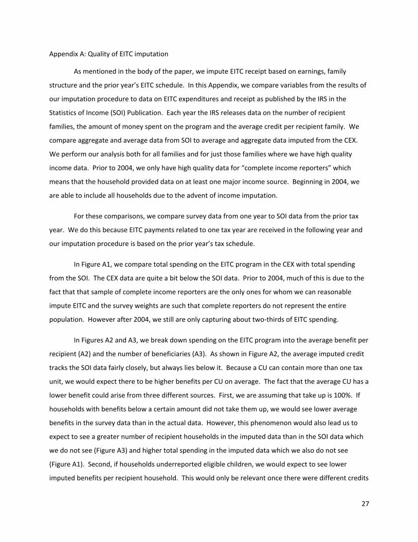
Appendix A: Quality of EITC imputation

As mentioned in the body of the paper, we impute EITC receipt based on earnings, family

structure and the prior year’s EITC schedule. In this Appendix, we compare variables from the results of

our imputation procedure to data on EITC expenditures and receipt as published by the IRS in the

Statistics of Income (SOI) Publication. Each year the IRS releases data on the number of recipient

families, the amount of money spent on the program and the average credit per recipient family. We

compare aggregate and average data from SOI to average and aggregate data imputed from the CEX.

We perform our analysis both for all families and for just those families where we have high quality

income data. Prior to 2004, we only have high quality data for “complete income reporters” which

means that the household provided data on at least one major income source. Beginning in 2004, we

are able to include all households due to the advent of income imputation.

For these comparisons, we compare survey data from one year to SOI data from the prior tax

year. We do this because EITC payments related to one tax year are received in the following year and

our imputation procedure is based on the prior year’s tax schedule.

In Figure A1, we compare total spending on the EITC program in the CEX with total spending

from the SOI. The CEX data are quite a bit below the SOI data. Prior to 2004, much of this is due to the

fact that that sample of complete income reporters are the only ones for whom we can reasonable

impute EITC and the survey weights are such that complete reporters do not represent the entire

population. However after 2004, we still are only capturing about two-thirds of EITC spending.

In Figures A2 and A3, we break down spending on the EITC program into the average benefit per

recipient (A2) and the number of beneficiaries (A3). As shown in Figure A2, the average imputed credit

tracks the SOI data fairly closely, but always lies below it. Because a CU can contain more than one tax

unit, we would expect there to be higher benefits per CU on average. The fact that the average CU has a

lower benefit could arise from three different sources. First, we are assuming that take up is 100%. If

households with benefits below a certain amount did not take them up, we would see lower average

benefits in the survey data than in the actual data. However, this phenomenon would also lead us to

expect to see a greater number of recipient households in the imputed data than in the SOI data which

we do not see (Figure A3) and higher total spending in the imputed data which we also do not see

(Figure A1). Second, if households underreported eligible children, we would expect to see lower

imputed benefits per recipient household. This would only be relevant once there were different credits

28

based on the number of children (1991-) or a credit for childless households (1994-). Prior to those

dates underreporting of children would influence eligibility, but not benefits given eligibility. Third, we

could see lower average benefits if there was misreporting of income. If income was underreported in

the phase in range, we would see lower imputed benefits. If income was over-reported in the phase out

range we would also see lower benefits.

When we display the imputed number of beneficiaries (A3), we see that this is also lower than

the number of beneficiary tax returns reported in the SOI. We would expect this prior to 2004, when we

cannot impute receipt for all people in the survey, but this pattern persists after 2004 as well. There are

also a number of forces that could be at work here. First, a CU can contain many tax units and more

than one tax unit may receive the EITC. In Figure A6, we display the number of tax units receiving the

EITC in our data. As mentioned in the body of the paper, we break CUs into tax units in order to

properly impute the EITC. This bias works in the correct direction, but is small. Second, households

could be misreporting the number of children. In particular, households with children may be reporting

that they don’t have children so our imputation procedure mistakenly labels them as ineligible.

Households may also report that they have fewer children than they have. Households with more

children receive EITC payments for a wider range of incomes. We do not think that the underreporting

of children in a major issue because the total number of children in the CEX is similar to the total

number in the US according to Census data. However, we may be incorrectly assigning some children to

tax units within the household. In particular, we could be assigning children to tax units with no earned

income or too high earned income while they belong in tax units with income within the EITC range.

However, this bias is likely to be small because most CUs only contain one tax unit. Third, tax units with

income may report that they have no income and therefore appear ineligible. Underreporting of

income among households with some income would make households more likely to be eligible for the

EITC not less likely. To investigate the role of income underreporting further, we compare pretax

income reported in the CEX to Census income data. In Figure A5, we display household median pre-tax

income by year according to the CEX and the Census. We chose to look at median income rather than

mean income because the CEX income data is top coded making mean comparisons inappropriate. This

graph shows some underreporting of income in the CEX.

Income underreporting can explain the patterns in Figures A2 and A3 if some CEX tax units

report having no income that have some income, and among households with income some in the

phase in range report having less income in the survey than they report to the IRS . Households

29

reporting having no income would lower our measure of the number of eligible households while

households reporting that they have less income in the phase in range would lower our estimate of

benefits given eligibility. This seems to be the explanation most consistent with the pattern in the data.

30

Figure A1: Total EITC Spending, IRS Statistics of Income vs. CEX Imputation

Note: Authors’ tabulations based on BLS, Various Years and IRS, Various Years.

Figure A2: Average Benefit, IRS Recipient Families vs. Eligible CEX Consumer Units


020

000

4000

060

000

1980 1990 2000 2010year

Spending (Millions), All CEX Spending (Millions), Complete CEX

Spending (Millions) IRS

050

010

0015

0020

00

1980 1990 2000 2010year

Average Credit, CEX Average Credit, Complete CEXAverage Credit, IRS

31

Figure A3: Number of Beneficiaries, IRS Returns vs. CEX Consumer Units


Figure A4: Number of Beneficiaries, IRS Tax Units, CEX Consumer Units and Tax Units


510

1520

2530

1980 1990 2000 2010year

Number of CU's with EITC Number of CU's with EITC, Complete

Number of Returns With EITC, IRS

510

1520

2530

1980 1990 2000 2010year

Number of CU's with EITC, Complete Number of Tax Units with EITC, Complete CEX

Number of Returns With EITC, IRS

32

A5: Median Household Pre-tax Income, Census vs. CEX

Note: Authors’ tabulations based on BLS, Various Years and data from the US Bureau of the Census, via Haver Analytics.

1000

020

000

3000

040

000

5000

0

1980 1990 2000 2010year

Median CU Income, All Median CU Income, Complete

Median Household Income: United States ($)

1

Working Paper Series

A series of research studies on regional economic issues relating to the Seventh Federal Reserve District, and on financial and economic topics.

Comment on “Letting Different Views about Business Cycles Compete” WP-10-01 Jonas D.M. Fisher Macroeconomic Implications of Agglomeration WP-10-02 Morris A. Davis, Jonas D.M. Fisher and Toni M. Whited Accounting for non-annuitization WP-10-03 Svetlana Pashchenko Robustness and Macroeconomic Policy WP-10-04 Gadi Barlevy Benefits of Relationship Banking: Evidence from Consumer Credit Markets WP-10-05 Sumit Agarwal, Souphala Chomsisengphet, Chunlin Liu, and Nicholas S. Souleles The Effect of Sales Tax Holidays on Household Consumption Patterns WP-10-06 Nathan Marwell and Leslie McGranahan Gathering Insights on the Forest from the Trees: A New Metric for Financial Conditions WP-10-07 Scott Brave and R. Andrew Butters Identification of Models of the Labor Market WP-10-08 Eric French and Christopher Taber Public Pensions and Labor Supply Over the Life Cycle WP-10-09 Eric French and John Jones Explaining Asset Pricing Puzzles Associated with the 1987 Market Crash WP-10-10 Luca Benzoni, Pierre Collin-Dufresne, and Robert S. Goldstein Prenatal Sex Selection and Girls’ Well‐Being: Evidence from India WP-10-11 Luojia Hu and Analía Schlosser Mortgage Choices and Housing Speculation WP-10-12 Gadi Barlevy and Jonas D.M. Fisher Did Adhering to the Gold Standard Reduce the Cost of Capital? WP-10-13 Ron Alquist and Benjamin Chabot Introduction to the Macroeconomic Dynamics: Special issues on money, credit, and liquidity WP-10-14 Ed Nosal, Christopher Waller, and Randall Wright Summer Workshop on Money, Banking, Payments and Finance: An Overview WP-10-15 Ed Nosal and Randall Wright Cognitive Abilities and Household Financial Decision Making WP-10-16 Sumit Agarwal and Bhashkar Mazumder

2

Working Paper Series (continued) Complex Mortgages WP-10-17 Gene Amromin, Jennifer Huang, Clemens Sialm, and Edward Zhong The Role of Housing in Labor Reallocation WP-10-18 Morris Davis, Jonas Fisher, and Marcelo Veracierto Why Do Banks Reward their Customers to Use their Credit Cards? WP-10-19 Sumit Agarwal, Sujit Chakravorti, and Anna Lunn The impact of the originate-to-distribute model on banks before and during the financial crisis WP-10-20 Richard J. Rosen Simple Markov-Perfect Industry Dynamics WP-10-21 Jaap H. Abbring, Jeffrey R. Campbell, and Nan Yang Commodity Money with Frequent Search WP-10-22 Ezra Oberfield and Nicholas Trachter Corporate Average Fuel Economy Standards and the Market for New Vehicles WP-11-01 Thomas Klier and Joshua Linn The Role of Securitization in Mortgage Renegotiation WP-11-02 Sumit Agarwal, Gene Amromin, Itzhak Ben-David, Souphala Chomsisengphet, and Douglas D. Evanoff Market-Based Loss Mitigation Practices for Troubled Mortgages Following the Financial Crisis WP-11-03 Sumit Agarwal, Gene Amromin, Itzhak Ben-David, Souphala Chomsisengphet, and Douglas D. Evanoff Federal Reserve Policies and Financial Market Conditions During the Crisis WP-11-04 Scott A. Brave and Hesna Genay The Financial Labor Supply Accelerator WP-11-05 Jeffrey R. Campbell and Zvi Hercowitz Survival and long-run dynamics with heterogeneous beliefs under recursive preferences WP-11-06 Jaroslav Borovička A Leverage-based Model of Speculative Bubbles (Revised) WP-11-07 Gadi Barlevy Estimation of Panel Data Regression Models with Two-Sided Censoring or Truncation WP-11-08 Sule Alan, Bo E. Honoré, Luojia Hu, and Søren Leth–Petersen Fertility Transitions Along the Extensive and Intensive Margins WP-11-09 Daniel Aaronson, Fabian Lange, and Bhashkar Mazumder Black-White Differences in Intergenerational Economic Mobility in the US WP-11-10 Bhashkar Mazumder

3

Working Paper Series (continued) Can Standard Preferences Explain the Prices of Out-of-the-Money S&P 500 Put Options? WP-11-11 Luca Benzoni, Pierre Collin-Dufresne, and Robert S. Goldstein Business Networks, Production Chains, and Productivity: A Theory of Input-Output Architecture WP-11-12 Ezra Oberfield Equilibrium Bank Runs Revisited WP-11-13 Ed Nosal Are Covered Bonds a Substitute for Mortgage-Backed Securities? WP-11-14 Santiago Carbó-Valverde, Richard J. Rosen, and Francisco Rodríguez-Fernández The Cost of Banking Panics in an Age before “Too Big to Fail” WP-11-15 Benjamin Chabot Import Protection, Business Cycles, and Exchange Rates: Evidence from the Great Recession WP-11-16 Chad P. Bown and Meredith A. Crowley Examining Macroeconomic Models through the Lens of Asset Pricing WP-12-01 Jaroslav Borovička and Lars Peter Hansen The Chicago Fed DSGE Model WP-12-02 Scott A. Brave, Jeffrey R. Campbell, Jonas D.M. Fisher, and Alejandro Justiniano Macroeconomic Effects of Federal Reserve Forward Guidance WP-12-03 Jeffrey R. Campbell, Charles L. Evans, Jonas D.M. Fisher, and Alejandro Justiniano Modeling Credit Contagion via the Updating of Fragile Beliefs WP-12-04 Luca Benzoni, Pierre Collin-Dufresne, Robert S. Goldstein, and Jean Helwege Signaling Effects of Monetary Policy WP-12-05 Leonardo Melosi Empirical Research on Sovereign Debt and Default WP-12-06 Michael Tomz and Mark L. J. Wright Credit Risk and Disaster Risk WP-12-07 François Gourio From the Horse’s Mouth: How do Investor Expectations of Risk and Return Vary with Economic Conditions? WP-12-08 Gene Amromin and Steven A. Sharpe Using Vehicle Taxes To Reduce Carbon Dioxide Emissions Rates of New Passenger Vehicles: Evidence from France, Germany, and Sweden WP-12-09 Thomas Klier and Joshua Linn Spending Responses to State Sales Tax Holidays WP-12-10 Sumit Agarwal and Leslie McGranahan

4

Working Paper Series (continued) Micro Data and Macro Technology WP-12-11 Ezra Oberfield and Devesh Raval The Effect of Disability Insurance Receipt on Labor Supply: A Dynamic Analysis WP-12-12 Eric French and Jae Song Medicaid Insurance in Old Age WP-12-13 Mariacristina De Nardi, Eric French, and John Bailey Jones Fetal Origins and Parental Responses WP-12-14 Douglas Almond and Bhashkar Mazumder Repos, Fire Sales, and Bankruptcy Policy WP-12-15 Gaetano Antinolfi, Francesca Carapella, Charles Kahn, Antoine Martin, David Mills, and Ed Nosal Speculative Runs on Interest Rate Pegs The Frictionless Case WP-12-16 Marco Bassetto and Christopher Phelan Institutions, the Cost of Capital, and Long-Run Economic Growth: Evidence from the 19th Century Capital Market WP-12-17 Ron Alquist and Ben Chabot Emerging Economies, Trade Policy, and Macroeconomic Shocks WP-12-18 Chad P. Bown and Meredith A. Crowley The Urban Density Premium across Establishments WP-13-01 R. Jason Faberman and Matthew Freedman Why Do Borrowers Make Mortgage Refinancing Mistakes? WP-13-02 Sumit Agarwal, Richard J. Rosen, and Vincent Yao Bank Panics, Government Guarantees, and the Long-Run Size of the Financial Sector: Evidence from Free-Banking America WP-13-03 Benjamin Chabot and Charles C. Moul Fiscal Consequences of Paying Interest on Reserves WP-13-04 Marco Bassetto and Todd Messer Properties of the Vacancy Statistic in the Discrete Circle Covering Problem WP-13-05 Gadi Barlevy and H. N. Nagaraja Credit Crunches and Credit Allocation in a Model of Entrepreneurship WP-13-06 Marco Bassetto, Marco Cagetti, and Mariacristina De Nardi

5

Working Paper Series (continued) Financial Incentives and Educational Investment: The Impact of Performance-Based Scholarships on Student Time Use WP-13-07 Lisa Barrow and Cecilia Elena Rouse The Global Welfare Impact of China: Trade Integration and Technological Change WP-13-08 Julian di Giovanni, Andrei A. Levchenko, and Jing Zhang Structural Change in an Open Economy WP-13-09 Timothy Uy, Kei-Mu Yi, and Jing Zhang The Global Labor Market Impact of Emerging Giants: a Quantitative Assessment WP-13-10 Andrei A. Levchenko and Jing Zhang Size-Dependent Regulations, Firm Size Distribution, and Reallocation WP-13-11 François Gourio and Nicolas Roys Modeling the Evolution of Expectations and Uncertainty in General Equilibrium WP-13-12 Francesco Bianchi and Leonardo Melosi Rushing into American Dream? House Prices, Timing of Homeownership, and Adjustment of Consumer Credit WP-13-13 Sumit Agarwal, Luojia Hu, and Xing Huang The Earned Income Tax Credit and Food Consumption Patterns WP-13-14 Leslie McGranahan and Diane W. Schanzenbach

Documents

The Earned Income Tax Credit and Food Consumption Patterns;