Arch. Hist. Exact Sci. (2010) 64:269–300DOI 10.1007/s00407-009-0056-z

The early application of the calculus to the inversesquare force problem

M. Nauenberg

Received: 10 December 2009 / Published online: 3 February 2010© The Author(s) 2010. This article is published with open access at Springerlink.com

Abstract The translation of Newton’s geometrical Propositions in the Principiainto the language of the differential calculus in the form developed by Leibniz and hisfollowers has been the subject of many scholarly articles and books. One of the mostvexing problems in this translation concerns the transition from the discrete polygonalorbits and force impulses in Prop. 1 to the continuous orbits and forces in Prop. 6.Newton justified this transition by lemma 1 on prime and ultimate ratios which wasa concrete formulation of a limit, but it took another century before this concept wasestablished on a rigorous mathematical basis. This difficulty was mirrored in the newlydeveloped calculus which dealt with differentials that vanish in this limit, and there-fore were considered to be fictional quantities by some mathematicians. Despite theseproblems, early practitioners of the differential calculus like Jacob Hermann, PierreVarignon, and Johann Bernoulli succeeded without apparent difficulties in applyingthe differential calculus to the solution of the fundamental problem of orbital motionunder the action of inverse square central forces. By following their calculations anddescribing some essential details that have been ignored in the past, I clarify the reasonwhy the lack of rigor in establishing the continuum limit was not a practical problem.

1 Introduction

At the beginning of the eighteenth century, the differential calculus in the form devel-oped by Leibniz was applied by his most prominent followers, Jacob Hermann, PierreVarignon, and Johann Bernoulli, to the fundamental problem of planetary motion—to

Communicated by Niccolò Guicciardini.

M. Nauenberg (B)Physics Department, University of California Santa Cruz, Santa Cruz, CA, USAe-mail: michael@physics.ucsc.edu

123

270 M. Nauenberg

describe the orbit of planets under the assumption that their motion is determined byan attractive force towards the Sun that varies inversely with the square of the distance.In 1679, Robert Hooke (Nauenberg 2005) wrote to Isaac Newton asking him

…and particularly if you will let me know your thoughts of that of compound-ing the celestiall motions of the planetts of a direct motion by the tangent & anattractive motion towards the centrall body (Newton 1960)

In the Principia, Newton took a great step forward by extending the application ofEuclidean geometry to the concept of force impulses which he represented by linesegments that in a limit have vanishing small magnitude,1 leading to the emergence ofa finite and continuous force. Such evanescent quantities appeared already in Greekgeometry, in the method of exhaustion which, for example, was applied by Archime-des to obtain a rigorous relations between the circumference and the area of a circle,as well as bounds for these quantities that he calculated algebraically.2

Shortly after the publication of the Principia in 1687, Leibniz applied Prop. 1 toderive the now well-known differential equation of motion for central forces in polarcoordinates. Then he gave an analytic proof that for elliptical orbital motion satisfyingKepler’s area law, the resulting force depends inversely on the square of the distancefrom the center,3 in accordance with Newton’s geometric proof in Prop. 11. Leibnizstimulated Johann Bernoulli and Pierre Varignon to apply the differential calculus tothe solution of propositions in the Principia, and Jacob Hermann (1710a, 1710b)4

used Cartesian coordinates instead of Leibniz’s polar coordinates to show that underthe action of inverse square forces, the orbit is a conic section. In Prop. 1, Newtondescribed the orbit for a general central force by a polygon, see Fig. 1, which Her-mann interpreted to be a sequence of chords of a continuous curve, see Fig. 2. Herepresented the Cartesian components of these cords by first-order differentials, andfound that the components of Newton’s line segments for the force impulses in Prop.1, introduced geometrically in the Principia, were second-order differentials.5 Given

1 In the seventeenth century, the concept of a differential or infinitesimal quantity was not well defined.Newton observed that

Fermat in his method de maximis et minimis & Gregory in his method of Tangents & Newton (in hismethod) of the first and last ratios use the letter o to signify a quantity not infinitely but indefinitelysmall & in this methods of tangents uses the letters a & e to become infinitely little…(Newton1968).

The most colorful characterization of infinitesimals was given by Bishop George Berkeley, who called them“the ghost of departed quantities” (Boyer 1989).2 Archimedes showed that the circumference c of a circle is proportional to its diameter d, and that thearea is proportional to the square of the diameter. He also calculated lower and upper bounds for the ratioc/d = π , namely, 223/71 < π < 22/7.3 Leibniz claimed that when he carried out his derivation he had not seen the Principia but only a reviewthat had appeared in the Acta Eruditorum. It has been shown, however, that Leibniz’s had obtained hisheavily annotate copy of the Principia before the publication of his work (Bertoloni Meli 1991).4 Hermann had been a student of Jacob Bernoulli in Basel where he learned the calculus in Leibniz’snotation.5 Whiteside claimed, however, that the sides of the polygons in Prop. 1 are second-order differentials(Newton 1974), but his incorrect analysis has been warmly endorsed by I. B. Cohen in his Guide to

123

The early application of the calculus 271

any dependence of the force impulse with the distance from the center of force, Her-mann obtained an exact algebraic relation of this second-order differential in terms ofquadratic terms of the first-order differentials which mirrored Newton’s geometricalrelation. For the case that the force impulses vary inversely with the square of thedistance, he solved his algebraic relation between finite differentials approximatelyby applying the rules of the differential calculus developed by Newton and Leibniz. Itwill be shown that a detailed study of Hermann’s work is an excellent introduction tothe calculus of differentials and its application to the solution of dynamical problemsas it was practiced in the early part of the eighteenth century.

In his response to Hermann, Bernoulli (1710) criticized his approach, claimingthat it was inadequate (Guicciardini 1999), and then he presented a different analyticmethod to evaluate the orbit for general central forces that was based on Newton’s Prop.41 integral. In a subsequent treatment, he also gave an alternate differential methodbased on Prop. 6 which will be shown to be equivalent to Hermann’s treatment, exceptthat in contrast with Hermann’s use of Cartesian coordinates, Bernoulli, like Leibnizbefore him, made use of polar coordinates. Guicciardini has remarked that Bernoulli’sevaluation of the integral in Prop. 41 for the case of an inverse square force was “theoutcome of a protracted and successful research on the application of Liebniz’s calcu-lus, most notably differential equations, to natural philosophy” (Guicciardini 2008).But in contrast to Herman, who based his method on the differential calculus, Bernoullievaluated the integral in Prop. 41 for the case of inverse square forces by methods ofalgebra and geometry that were already familiar to mathematicians in the seventeenthcentury including Fermat, Huygens, Newton, and Pascal (Boyer 1989; Kline 1972).

In the next section, I discuss Herman’s analysis in Cartesian coordinates in somedetail, because it is the simplest and most straightforward application of the differentialcalculus to the solution of the problem of planetary motion formulated geometricallyin Newton’s Principia. A new result that emerges from this discussion is the con-nection of Hermann’s first integral to Newton’s geometrical construction in Prop. 17.In Sect. 2, I describe the corresponding derivation in polar coordinates by Leibniz’swhich apparently even Newton had some difficulties to understand.6 In Sect. 3, I dis-cuss the analysis of BernoulIi and Varignon who also represented differentials in polarcoordinates, but instead of treating the force by a sequence of discrete impulses, theybased their treatment on a representation of a continuous force in terms of the radiusof curvature of the orbit which had been obtained in differential form by Bernoulli.7

The method employed by Bernoulli and Varignon, was based on an expression forthe force in terms of the radius of curve communicated by d’Moivre to Bernoulli in1706. Newton, who had derived this expression earlier, included it in the 1713 edi-

Footnote 5 continuedNewton’s Principia (Cohen 1999). Evidently, in the eighteenth century, Newton’s limiting procedures werebetter understood than in our present time. A detail discussion of Prop. 1 is given in reference (Nauenberg2003).6 Newton claimed erroneously that Leibniz had made an error in handling second-order differentials in hisequation.7 Bernoulli’s differential expression for the curvature first appeared in section 78 of L’Hospital textbookof the calculus Analyse des Infiniment Petits pour L’Intelligence des Lignes Courbes.

123

272 M. Nauenberg

Fig. 1 Newton’s diagram forProp. 1, Book 1 of the Principia

tion of the Principia, in a revised version of Prop. 6 that contained several additionalcorollaries. In Sect. 4, I discuss Bernoulli’s solution based on Prop. 41, and describea geometrical representation which he developed to present his result, followed by aproof that this representation corresponds to the algebraic equation for conic sectionsin Cartesian coordinates.8 Section 5 contains some conclusions followed by Appendix1 on the early derivation of the fundamental theorem of the calculus, and Appendix2 on a succint derivation with the aid of vector calculus of the results in the previoussections.

2 Hermann’s solution for the inverse square force problem

Hermann’s solution (1710a, 1710b) of the inverse problem of dynamics—given acentral force to obtain all the orbits satisfying Kepler’s area law—was based on therepresentation in Cartesian coordinates of Newton’s geometrical construction in Prop.1, Book 1 of the Principia, and on the application of the differential calculus.9 InProp. 1, Newton gave a proof that under the action of a continuous central force, abody moves in a planar orbit, and the “areas describe by radii drawn to the center offorce are proportional to the times”. Newton started the proof of this proposition byassuming that the force consisted of a sequence of impulses in a plane directed towardsa common center at equal time intervals. Then, in between impulses, the motion takesplace along straight lines with constant velocity shown in his diagram, Fig. 1., as thepolygon with sides AB, BC , etc. At each vertex of this polygon, Newton compounded

8 For another discussion of the contributions of Leibniz, Bernoulli, Hermann, and Varignon to the inverseproblem of central forces, see references Guicciardini (1999), Aiton (1962), and Aiton (1954).9 The source of Hermann’s diagram has been either neglected (Mazzone and Roero 1997; Bernoulli 2008)or errorneously assumed to be based on Prop. 6 of the Principia (Guicciardini 1999; Wilson 1994).

123

The early application of the calculus 273

Fig. 2 Herman’s geometricalconstruction for an orbit forcentral forces

the previous velocity with the instantaneous change of velocity due to a force impulsedirected towards the center at S. For example, in Fig. 1 the effect of an impulse at Bis described by a short line Cc parallel to BS, where c is the position at the end ofthe time interval in the absence of the impulse, found by extending the line AB by anequal length Bc. Then Newton showed that the area of the triangles ASB and BSCare equal, and repeated this construction in sequence at each vertex of the polygon.10

He considered a continuous force to be the limiting case of a discrete sequence of suchimpulses as the time interval between these impulses becomes vanishingly small. Cor-respondingly, the areas of the triangles which are proportional to these time must alsobecome vanishingly small. In order to indicate how such a limit could be approachedgeometrically, Newton referred to Lemma 3, Cor. 4 which presupposed the existenceof a continuous curve such that the vertices of the polygon lie on the curve and thesides of the polygon are the chords of arcs of this curve. In this case, for each timeinterval, the magnitude of the displacements due to the force impulses are uniquelydetermined. In Lemma 11, Newton gave a proof that for such a limit to exist, the curvemust have a finite radius of curvature.

In his diagram, Fig. 2, Hermann reproduced the first two vertices of the polygonin Prop. 1, but he turned the counter clockwise direction of rotation on this polygonaround the center of force at S into a clockwise rotation. To represent Newton’s geo-metrical construction algebraically, Hermann introduced Cartesian coordinates, andobtained an expression for the force impulse E D in terms of a second-order differen-tial. It will be shown that Hermann’s equations are exact algebraic relations betweendifferentials, but that his two-step integration procedure to solve these equations forthe case of an inverse square force involve approximations in that higher order differ-entials are neglected, in accordance with the rules of the differential calculus rules.These rules were formulated in the same form by Newton and by Leibniz.11

10 Since the time interval to travel along Bc and BC are the same, it appears that the time interval to travelalong Cc must vanish. To consider the continuum limit, however, Newton treated this time interval as asecond-order differential.11 By 1669, Newton had developed the differential form of the calculus, but his manuscript where circu-lated only privately by John Collins and were not published until 1711. Excerpts from the letter that Newton

123

274 M. Nauenberg

In his letter to Bernoulli, Hermann did not mention the origin of his geometricalrepresentation of central forces, Fig. 2, but in a more detailed article in the Giornalede’Letterati d’Italia (Hermann 1710b), he acknowledged that it came from Newton’sProp. 1. By including in his diagram an orbital curve which was absent in Newton’sdiagram, Hermann showed explicitly how to obtain a continuous force as a limit offorce impulses when the triangles associated with this construction are made vanish-ingly small.12 Hermann’s method is equivalent to an earlier derivation by Leibniz, alsobased on Prop. 1,13 who used polar coordinates in his derivation of a second-orderdifferential equation for central forces. In his response letter to Hermann, Bernoullialso obtained Leibniz’s differential equation in polar coordinates, but this derivation,which I will discuss below, was straightforward because it was based on a differentialexpression for the radius of curvature that he had obtained previously.

In Hermann’s diagram, which consists of a segment of three consecutive verticesof the diagram associated with Prop. 1, the curve ABC D represents an orbit, thecenter of force is at S, and the line L E is obtained by extending the chord betweentwo nearby points B and C on this curve on one side to E , where C E = C B, andon the other side to L at the intersection of L E with a horizontal line L I . The lineL I is the x-axis for a Cartesian coordinate system x, y, with the origin at S, whichintersect the curve ABC D at A. In this Cartesian representation, the coordinates ofC and B are x = SI, y = C I , and x − dx, y − dy, respectively, where dx, dy arefirst-order differentials dx = B H and dy = C H . The radial line C S completes thetriangle C SB, and its area in terms of the Cartesian coordinates can be shown tobe (1/2)(ydx − xdy). In Prop. 1, Newton gave a geometrical proof that under theaction of a central force, with center at S, this area is proportional to the time inter-val dt for a body to move from B to C . Following Newton’s demonstration, in theabsence of a force, a body would move, from C to E during a second equal timeinterval dt . But when a force impulse towards S occurs at B, the next location of thebody is at D on the curve ABC D, where its location is obtained by drawing fromE a line DE that is parallel to C S intersecting the curve. According to Prop. 1, thelength of the segment DE is a measure of the magnitude of the central force impulse

Footnote 11 continuedsent to Leibniz via Oldenburg and further material sent by Newton appeared in volume 2 of Wallis’s Opera(1693) (Guicciardini 2009). Some of the principal concepts, however appeared in Lemmas in Sect. 1, Book1, and in Lemma 2, Book 2 of the Principia. Leibniz published his first results in 1684 in the Acta Erudi-torum, and he had contacts with the Johann and Jacob Bernoulli who promoted the early dissemination ofthe calculus in the Continent.12 In Newton’s words, “Now let the number of triangles be increased and their width decreased indefinitely,and their ultimate perimeter ADF will (by lemma 3, corol. 4) be a curved line”. In Hermann’s diagram,Fig. 2, this limit “curved line ” is ABC D, the center of force is at S, the central force impulse at B is DE ,and two of Newton’s triangles of equal area are BC S and C DS. In the diagram associated with Prop. 1, alimit curve is not drawn, but its existence is implied by Newton’s reference to lemma 2, corol. 4. Indeed,such a curve is essential to specify Newton’s geometrical construction when “‘the number of triangles beincreased…indefinitely” (Nauenberg 2003). Although the necessity for assuming such a curve escaped theattention of contemporary commentators of Prop.1, it was recognized first by Leibniz and then by Hermanin his diagram which represents the essential features of this proposition.13 Leibniz claimed that he had obtained his result before he had seen a copy of the Principia, but hisheavily annotated copy of Newton’s has been found to pre-date his work (Bertoloni Meli 1991; Leibniz1973), demonstrating a remarkable lack of candor on his part.

123

The early application of the calculus 275

at B, and the object of Hermann’s diagram was to express this magnitude in termsof differentials. Representing the Cartesian coordinates of D by x + dx′, y + dy′,where dx′ = C K , and dy′ = DK , the line segments DF and E F = representingthe Cartesian components of DE are determined by the second-order differentialsDF = −ddx = dx − dx′, and E F = −ddy = dy − dy′.14 It is important to rec-ognize that in contrast with the first-order differentials dx, dy, where either one or acombination of the two can be chosen as an arbitrary small quantity, the subsequentdifferentials dx′, dy′ are both determined, when a curve ABC D is assumed to be given.Hence, the second-order differentials ddx, ddy also depend on the magnitude of thesefirst-order differentials.15 Geometrically, this dependence is evident from Herman’sdiagram, Fig. 2, which shows that the position of D on the curve ABC D dependson the value chosen initially for x and dx. The object of the differential calculus isto find this curve given, the dependence of the central force f on the distance C S,e.g., for an inverse square force, f ∝ 1/C S2. By similarity of the triangles EDF andCSI ,

E D = ddx

√x2 + y2

x. (1)

Assuming that the orbital curve ABC D has a finite curvature, Newton gave a proofin Lemma 11 of Book 1 of the Principia that the magnitude of the force impulse E Ddepends quadratically on the length BC = √

dx2 + dy2. Since the time interval dtis proportional to the area of the triangle C BS= (1/2)|xdy − ydx|, which dependlinearly on dx and dy, the ratio E D/dt2 has a finite limit when dx, dy become van-ishingly small. In Prop. 6, Newton defined a continuous force f by the relation (seeFig. 4)

f ∝ Q R

(S P × QT )2(2)

where Q R = (1/2)E D and S P × QT corresponds to twice the area of the triangleC BS, in the limit that the triangle C BS becomes vanishingly small. Substituting Her-mann’s second-order differential expression for E D, Eq. 1, in Newton’s relation forthe force, Eq. 2, leads to an expression for the force

f ∝ −ddx√

x2 + y2

x(ydx − xdy)2, (3)

where the minus sign appears when f is an attractive central force.

14 In section IV of the Analyse des Infinitment Petits, second-order differentials are defined as the differencebetween two consecutive first-order differentials, in accordance with Hermann’s application.15 At this stage, it should become clear why Hermann’s analysis required three adjacent vertices from thepolygon in Prop. 1, because a second-order differential like ddx is determined by the difference of twoadjacent first-order differentials, dx and dx′.

123

276 M. Nauenberg

For an inverse square force, f ∝ 1/(x2 + y2), Herman then obtained an equationfor the second-order differential ddx in the form

ddx = x(ydx − xdy)2

a(x2 + y2)3/2, (4)

where a is a constant with the dimensions of length, introduced to convert Newton’sproportionality relation for force, Eq. 2 into an equality.16 Such an algebraic relationbetween first- and second-order differentials, however, remains undetermined until afurther condition is imposed on the first-order differential dx and dy, because thesedifferentials cannot be varied independently. Hermann’s relation was obtained fromProp. 1 geometrical construction which leads to the constraint that the first-order dif-ferential ydx − xdy is a constant, that is

d(ydx − xdy) = 0. (5)

This condition implements in differential form Kepler’s area law which, in Prop. 1,Newton had shown to follow from central forces, and Hermann’s differential relation,Eq. 4, was derived by applying this constraint.17 To integrate18 his differential relation,Hermann had to impose this condition which then becomes an additional second-orderdifferential relation which he applied implicitly in his integration of Eq. 4.

In his treatment, Hermann neglected to consider an equivalent representation forf obtained by substituting for E D in Eq. 2 the expression obtained in terms of thesecond-order differential ddy,

E D = ddy

y

√x2 + y2. (6)

When substituted in Newton’s relation for the force, Eq. 2, this expression leads to theequivalent relation

f ∝ − ddy√

x2 + y2

y(ydx − xdy)2, (7)

16 For an elliptic orbit, the constant a is the latus rectum of the ellipse. Setting ydx − xdy = ldt andf = μ/(x2 + y2), where l is the angular momentum, and μ is the strength of the inverse square force,leads to the relation a = l2/μ that determines the value of a.17 For central forces, this condition corresponds to the conservation of angular momentum l, which in New-ton’s fluxional calculus, as well as in modern calculus, is represented by l = yx−xy, and l = yx−xy = 0,The dot superscript corresponds to a derivative with respect to time.18 In Leibniz’s calculus, to integrate a relation between differentials meant to find a relation between dif-ferentials of a lower order which satisfies the requisite relation between the higher order differentials. Bythe fundamental theorem of the calculus, this operation corresponds to the calculation of the area under agiven curve (see Appendix 1). It should be pointed out that without specifying the first-order differentialsin the problem that are kept fixed, the concept of a second order or higher order differential is meaningless.In Hermann’s calculations, the linear combination of differentials ydx − xdy ∝ dt is kept fixed.

123

The early application of the calculus 277

and for an inverse square force, f = 1/(x2+y2), leads to the second-order differentialrelation

ddy = −y(ydx − xdy)2

a(x2 + y2)3/2, (8)

which is analogous to Eq. 4, and must also be satisfied. By multiplying Eq. 4 by y andEq. 8 by x, one finds that the condition

xddy − yddx = d(xdy − ydx) = 0 (9)

is then automatically satisfied when both Eqs. 4 and 8 are valid. Actually, this result isa straightforward proof, based on the application of the differential calculus, of New-ton’s theorem in Prop. 1 that “…equal areas are described during equal time intervals”.But Hermann missed this simple proof, and it took another 6 years before he cameup with a different and rather convoluted proof (Guicciardini 1999) that was basedon the expression for the force in terms of the radius of curvature of the orbit. Thisalternate expression for the force appeared for the first time in the second edition ofthe Principia, and it was derived by Bernoulli who in turn had learned it from a privatecommunication by De Moivre (Guicciardini 1999)

For the first integral of his second-order differential relation, Eq. 4, Hermann set(ydx − xdy) equal to a constant and obtained

dx = y(ydx − xdy)

a√

x2 + y2. (10)

But to establish this result, an essential approximation was to neglect all higher orderterms in the differentials dx, and dy that appear in the calculation of the differentialon the right hand side of his relation. It is instructive to examine this step in somedetail, because it illustrates the treatment of differentials in the calculus of Newtonand Leibniz, and the nature of the approximations that are made at each step in itsimplementation.

The differential of the product of two quantities u, v is, by definition,

d(uv) = (u + du)(v + dv)− uv = udv + vdu + dudv, (11)

but the assumption that du and dv are small quantities which ultimately vanish, impliesthat in this limit the product dudv can be neglected compared to the terms linear indu and dv, that is

d(uv) ≈ udv + vdu. (12)

I have introduced here the sign ≈ to indicate that this relation is an approxima-tion.19 It is the basis of the differential calculus of Newton and Leibniz, and appears

19 For finite values of du and dv, the common use of the equality sign, which unfortunately is standardform in the literature on this subject, leads often to confusion.

123

278 M. Nauenberg

prominently as Prop. II in L’Hospital 1696 book, Analyse des Infinitiment Petits, thefirst text-book on this new calculus. The justification given for neglecting dudv is that

…dudv is a quantity infinitesimally small compared to the other terms udv, andvdu; because if one divides, for example, udv and dudv by dv, one finds on theone hand u, and on the other du that is its differential, and consequently it isinfinitesimally smaller than it.20

For Hermann’s problem, let u = y, v = 1/√

x2 + y2, then the next step is toobtain an approximation for the differential dv. Setting z = 1/v, and applying repeat-edly the basic calculus rule, Eq. 12, one finds dz2 ≈ 2zdz ≈ 2(xdx + ydy) or dz ≈v(xdx + ydy), and since d(zv) = 0, dv ≈ −v2dz ≈ −v3(xdx + ydy). Hence

udv ≈ −y(xdx + ydy)

(x2 + y2)3/2, (13)

vdu = dy(x2 + y2)

(x2 + y2)3/2, (14)

and finally

d(uv) = d

(y

√x2 + y2

)

≈ x(xdy − ydx)

(x2 + y2)3/2, (15)

which verifies that Eq. 10 is the first integral of Eq. 4. Actually, the differential dv is apower series expansion, which according to Newton’s generalized binomial theorem,consisted of an infinite number of terms of higher powers in dx and dy. But a proofthat the infinite sum of all these neglected terms is of higher order and therefore canbe neglected, was not available. Hence, for a finite value of dx, d(uv)dt ≈ addx,and for finite differentials Eq. 10 satisfies Eq. 4 only approximately. But in accordancewith the fundamental theorem of calculus, in the limit that dx becomes vanishinglysmall,21 Eq. 10 is an exact integral of Eq. 4.

In a similar way, Herman found that the integral of Eq. 10 is

a

x=

√x2 + y2

x± c, (16)

20 …dudv est une quantité infiniment petit par rapport aux autres terms udv & vdu; car si l’on divise,par example, udv & dudv par dv, on trouve d’une part u, & de l’autre du qui en est la différence, & parconséquent infinitment moindre qu’elle.21 Regarding the approximations in relations involving finite differentials, Leibniz commented that

at the same time one has to consider that these ordinary incomparables themselves are by no meansfixed or determined; they can be taken as small as one wishes in our geometrical arguments. Thusthey are effectively the same as rigorous, infinitely small quantities, for if an opponent would denyour assertion, it follows from our calculus that the error will be less than any error which he will beable to assign, for it is in our power to take the incomparably small small enough for that, as onecan always take a quantity as small as one wishes (Bos 1973).

123

The early application of the calculus 279

where c is a constant.22 Again, this result can be verified by taking differentials onboth sides of this relation, applying the Kepler area law condition (conservation ofangular momentum), Eq. 9, and keeping only terms that appear in the resulting seriesexpansion that are first order in the differentials dx and dy. This relation is the alge-braic equation for a conic section.23 with eccentricity c; a parabola for c = 1, anellipse for c < 1, and a hyperbola for c > 1. For an ellipse, the constant a is thelatus rectum, and a/(1 − c2) is the major axis, providing the role of unit of lengthto the constant a introduced by Hermann. Hermann’s solutions constrain the axis ofthe conic to lie along an arbritraly chosen horizontal, but this restriction is invalid forarbitrary initial values of position and velocity. But by including in the first integral,the missing constant of integration e(yx−xdy) pointed out by Bernoulli, one obtainsthe solution for a general conic section

a =√

x2 + y2 + cx + ey (17)

It is instructive to apply the differential calculus to obtain the solution of the directproblem in dynamics—given a planar orbit satisfying Kepler’ area law, to obtain theradial dependence of the central force. In Props. 11–13, Newton gave a geometricalproof that for orbits that are conic section, the force depends inversely with the distancefrom a center. Starting with the Cartesian coordinate representation of a conic sectiongiven in Eq. 16, and taking his differential steps in reverse order by applying repeat-edly the chain rule to this representation, leads to the expressions for the first- andsecond-order differential dx, Eq. 10, and ddx, Eq. 4, provided that the area ydx−xdyof the triangle BSC is kept constant.24 In Cartesian coordinates, Eq. 3 corresponds toNewton’s definition for a central force f given in Prop. 1 and Prop. 6, and substitutingfor ddx in this equation the relation given by Eq. 4 yields for the force the inversesquare radial dependence, f ∝ 1/(x2 + y2).

22 The ± sign corresponds to the two possible choices for the foci of a conic section as the center of theinverse square force.23 In his evaluation, Herman introduced a spurious constant b, describing his result by the value of a con-stant c/b, “…qui est une équation aux trois Sections Conique; savoir à la Parabole si b = c, à l‘Ellipse sib > c, & à l‘dHyperbole si b < c”.24 The first-order differential of the algebraic equation for a conic section, Eq. 16, including an additionalterm ey, where e was a constant pointed out by Bernoulli is

da = xdx + ydy√

x2 + y2+ cdx + edy. (18)

and since a is a constant da = 0 Setting ydx − xdy = dt , where dt is treated as a constant when taken adifferential of this relation, one obtains an equation for dx by substituting dy = (1/x)(ydx − dt) in thisequation,

(

√x2 + y2 + cx + ey)dx = ydt

√x2 + y2

+ edt. (19)

But for the conic section, Eq. 16, the coefficient of dx is equal to a, which shows that this equation corre-sponds to Hermann’s first integral, Eq. 10 including a missing constant of integration.

123

280 M. Nauenberg

Bernoulli responded to Hermann with a harsh criticism of his work Bernoulli (1710),remarking that Hermann had not provided any direct procedure to obtain the first inte-gral, Eq. 10, of his second-order differential equation, Eq. 4 and that he had obtainedhis result because he already knew the answer—that his second integral was a conicsection, Eq. 16. Actually in practice, integration of a nonlinear differential equationby an application of the fundamental theorem of the calculus usually involves an edu-cated guess of the solution, followed by the verification that its derivative satisfies thedifferential equation.25 Bernoulli also pointed out that in the first integration Hermannhad neglected to include a constant term. This term has to be a first-order differential,and since ydx − xdy is treated as a constant, it has the unique form e(ydx − xdy),where e is an additional constant of integration. For this reason, Bernoulli stated that“one might be left in doubt that there is another kind of curve, other than the conic sec-tions, that satisfies your problem”, claiming that Herman had failed to prove that conicsections were a unique solution of his differential relation. Then Bernoulli showed thathis constant leads to an additional term of the form ey/x on the right hand side ofHerman’s second integral, because

d(y/x) ≈ − 1

x2 (ydx − xdy). (20)

It can be verified that with this additional term, Eq. 16 leads to the algebraic equa-tion for a conic section with its major axis rotated relative to the x-axis by an angleω = atan(e/c). Ironically, Bernoulli’s own proof that the solution he obtained froman application of Prop. 41 in Newton’s Principia satisfied the algebraic equation fora conic section also was restricted to the special case that e = 0, as will be shown inthe next section.

Setting dt = (1/ l)(ydx − xdy), where l is a constant correspond to the angularmomentum, indicates that Herman’s first integral, Eq. 10, with the additional constante introduced by Bernoulli, can be written in the alternate form

e = a

lvx − y

√x2 + y2

, (21)

where vx = dx/dt is the x component of the velocity v. If Herman had also solvedfor vy = dy/dt , where vy = (y/x)vx − l/x, according to Kepler’s area law, he wouldhave found that

c = −a

lvy − x

√x2 + y2

, (22)

Hence, given the position x, y relative to the center of force, and the velocity vx, vyat some point along the orbit, called the initial conditions, the angular momentumconstant l = yvx − xvy is fixed and all the parameters of the conic section are deter-

25 For this purpose, both Newton and Leibniz created extensive tables of derivates of elaborate functions,and ever since such tables have become a standard aid for the analytic evaluation of difficult integrals.

123

The early application of the calculus 281

mined in units of Hermann’s length parameter a. In this form, Herman’s result can berecognized as the components of a vector

�ε = �v × �lμ

− �rr

(23)

where �l is the vector angular momentum taken normal to the plane of the orbit along thenegative z axis (Herman’s diagram corresponds to clockwise rotation around the centerof force S), and μ = a/ l2 is a constant that determines the magnitude of the inversesquare force, f = μ/(x2 + y2). This vector �ε is a constant of the motion directedalong the axis of conic section with a magnitude corresponding to its eccentricity ε,where εx = c, and εy = e. Ninety one years later, it was derived in a similar mannerby Simon Pierre Laplace (1798) who apparently was unaware of Herman’s result.Actually, this special invariant of the motion for inverse square forces had alreadybeen described in geometrical form by Newton in the Principia, Book 1, Prop. 17, butthis connection has not been made in the past. In this way, Prop. 17 establishes theuniqueness of conic sections, a fact that was already recognized by Euler (1736), butstill leads to misconceptions up to the present time. In the first edition of the Principia,Newton gave an argument for the uniqueness of conic sections in Cor. 1 to Prop. 13which was considered to be insufficient and lead to disputes. But in the second edition,Newton added the remark that

For if the focus and the point of contact and the position of the tangent are given,a conic can be described that will have a given curvature at that point. But thecurvature is given from the given centripetal force and velocity of the body,and two different orbits touching each other cannot be described with the samecentripetal force and the velocity.

In the differential calculus, the uniqueness of the conic section solution for inversesquare force is based on the fundamental theorem of the calculus (see Appendix 1).

3 Leibniz differential equation for motion in polar coordinates

In 1688, after studying the Principia, Leibniz’s was able to apply his calculus toobtained the differential equation of motion for central forces in polar coordinateswhich appeared in his Tentamen de motuum coelestium causis (Bertoloni Meli 1991).Like Hermann’s derivation, Leibniz’s treatment was also based on Newton’s Prop. 1.For clarity, in Fig. 3 taken from E. J. Aiton (1995), I show only the section of Leib-niz’s diagram relevant to his analysis, which is also similar to Hermann’s diagram,Fig. 2. The curve M1,M2,M3 represents the orbit of planet moving under the actionof a force centered at the point indicated here by the symbol for the Sun (a circlewith a small dot in the center which will be called S here). Leibniz draws the chordM1 M2 which he extends by an equal length to a point L , and from there draws the linesegment L M3, parallel to the radial line M2S that intersects the curve at M3. In thisway, given any two nearby points M1 and M2 on the curve, the location of the thirdpoint M3 is determined. Hence, except for change in notation, Leibniz’s construction

123

282 M. Nauenberg

Fig. 3 A section of Leibnizdiagram

corresponds to Newton’s construction in Prop. 1, shown in Fig. 1. The only differenceis that Leibniz changed the sense of rotation in the Prop. 1 diagram to a clock-wiserotation, in the same manner that Hermann did later on in his diagram, Fig. 2.

The additional lines in Leibniz’s diagrams are auxiliary lines to derive the necessaryrelations among the differentials. The lines M1 N and M3 D2 represent differential nor-mals to the radial line SM2 drawn from the vertices M1 and M3, respectively, and M1 Pand M3T2 are corresponding differential arcs centered at S. In addition, a line M3Gis drawn parallel to M2L . Then setting SM1 = r − dr, SM2 = r and SM3 = r + dr ′,

dr = −(P N + N M2) (24)

is the differential change in the radial coordinate from M1 to M2, and

dr ′ = −M2T2 = −(L M3 + G D2 − T2 D2). (25)

is the corresponding change from M2 to M3. By equality of the triangles M1 M2 N andM3 D2G, N M2 = G D2, and P N = D2T2. Hence

dr ′ = −(L M3 + N M2 − P N ) (26)

and

ddr = dr ′ − dr = −L M3 + 2P N (27)

where

P N = (M1 N )2

2SM2. (28)

123

The early application of the calculus 283

to second order in M1 N . Since Leibniz followed Newton’s geometric construction inProp. 1, the triangles M1SM2 and M2SM3 have equal areas� = (1/2)(M1 N ×SM2),and the elapsed time interval dt satisfies Kepler’s area law dt = (1/a)�. Here a is aconstant of proportionality introduced by Leibniz on dimensional grounds which werecognize as the angular momentum for unit mass. Setting SM2 = r , and M1 N =adt/r , one obtains

P N = a2dt2

2r3 , (29)

Substituting in Eq. 27 this expression for P N and L M3 = f dt2, where f is the centralforce, Leibniz obtained the now well-known differential equation of motion in polarcoordinates,

ddr − a2dt2

r3 = − f dt2 (30)

Leibniz also demonstrated that when the orbital curve is an ellipse and the motionsatisfies Kepler’s area law, d� = 0, the force f is an inverse square force f ∝ 1/r2.His proof, which he obtained by evaluating the second-order differential ddr from afirst-order differential expression for the elliptical orbit (Aiton 1995), corresponds toNewton’s geometric proof in Prop. 11.

It has been argued that Leibniz’s representation of orbits by discrete polygonsinstead of continuous curves was just a matter of convenience (Aiton 1962; BertoloniMeli 1991; Guicciardini 2008), but this is not the case. In Prop. 6, Newton representeda segment of the orbit by an arc, P Q, and the force by the deviation Q R from a lineZ P RY tangent at one end P of the arc, Fig. 4. In order to apply the differential calculusto this representation, however, an analytic expression for this tangent line is required,but this is an unknown quantity which cannot be expressed in terms of differentialsfrom the geometric quantities given in Prop. 6. In fact, three nearby points of the orbitare required to obtain a unique circular arc, and then the tangent line at any point onthis arc can also be obtained. Such a construction was pointed out to Leibniz by PierreVarignon, and if the tangent line is placed midway on the arc, it leads to half as large avalue for the force impulse obtained by Leibniz and by Hermann (Guicciardini 2008).This procedure is equivalent to Leibniz’s original construction, Fig. 3.26

Although Leibniz derived his analytic equation of motion directly from Newton’sgeometrical construction in Prop. 1, he gave it a completely different physical inter-pretation. Regarding the issue of how mathematics can mirror reality, it is of interestto discuss Leibniz’s interpretation, because it illustrates ambiguities that can occur atthe initial stages when a new theory is in the first stage of development. Following

26 In the second edition of the Principia, Newton altered Prop. 6 to read

…the sagitta of the arc is understood to be drawn so as to bisect the chord and, when produced,to pass through the center of force…

This sagitta is the displacement associated with the force, which corresponds to Varignon’s construction,but Newton did not alter the diagram, Fig. 4, associated with Prop. 6 accordingly.

123

284 M. Nauenberg

Fig. 4 Newton’s diagram forProp. 6, Book 1 of the Principia

the Cartesian argument that planets rotate around the sun because they are carried byvortices of unseen particles or a fluid circulating the sun, Leibniz argued that Kepler’sarea law gave a mathematical description of these vortices, namely, that the circulationvelocity of a vortex depends inversely with the distance from the sun. A consequenceof Leibniz’s interpretation is that planets experience an acceleration or force which,in accordance with Prop. 2 in the Principia27 is directed towards the sun, and is repre-sented by L M3 in Leibniz’s diagram, Fig. 3, but Leibniz did not give any justificationthat this force must be a central force. For circular motion, this central force whichLeibniz re-named solicitation of gravity is balanced by an outward centrifugal conatusrepresented by the term a2dt2/r3 in Leibniz’s equation of motion, Eq. 30. Leibnizinterpreted this term as a real force due to the Cartesian vortices acting on the planet,which depends on the parameter a. Since the rotational velocity of the planet is thesame as that of the vortex, a is also an intrinsic property of the planet corresponding toit angular momentum. Planets, however, do not rotate in circular orbits, as would beexpected in this Cartesian model, but instead move in elliptical orbits crossing differ-ent vortices, and Leibniz explained the variation in radial distance, expressed by thesecond-order differential ddr , by the difference between the solitication of gravity andthe centrifugal connatus. But this radial acceleration is also a consequence of Prop.1, and it does not require the existence of vortices. In fact, such an explanation forthe radial oscillations in the orbit was already given by Newton in a cryptic remark inhis 1679 correspondence with Hooke, and in his 1681 correspondence with Cromptonregarding a question of Flamsteed about the motion of comets near the sun (Nauenberg(1994)). The vortex interpretation had one advantage over Newton’s theory, becauseit offered an explanation why the planets all rotated along the same direction.28 Butthis explanation had to be abandoned when comets were found to rotate around thesun in directions opposite to that of the planets.29

27 In Prop.2, Newton gives a proof that “every body…that describes areas around a point proportional tothe times, is urged by a centripetal force toward the same point”. But Newton’s proof is based on the conceptof inertial straight line motion in the absent of an external force, which Leibniz ignored.28 The modern explanation is based on the theory for the origin of the planets from an initial dense gasof particles circulating the sun which holds also for numerous recently discovered extrasolar planetarysystems.29 It is interesting to compare the seventeenth century vortex theory based on unobserved particles withour current speculations of dark matter. This matter, which is also associated with unobserved particles, hasbeen invoked to account for the peculiar rotational velocity of some stars that cannot be explained with ourcurrent theory of gravity by the amount of observable matter in galaxies.

123

The early application of the calculus 285

4 Bernoulli’s and Varignon’s derivations of Prop. 39 and 41.

In his response letter to Hermann (Bernoulli 1710), Bernoulli applied the differentialcalculus to derive Newton’s expression for the energy conservation principle, Prop.39, and the integral for the orbital curve in polar coordinates, Prop. 41, for a generalcentral force. A similar derivation was given by Varignon in the same issue of theMemoires of the Academy des Sciences where the letters of Hermann and Bernoulliappeared. Varignon’s derivation differs from Bernoulli’s only in the form that eachone used for the central force. In 1706, Bernoulli learned the expression for a centralforce in terms of the radius of curvature ρ of the orbit from a correspondence withDe Moivre, although he did not acknowledge it (Guicciardini 2008).30 On the otherhand, by following Newton’s geometrical derivation of Prop. 39, Varignon obtained anexpression for the force in terms of the second-order differential of the arc length of theorbit. Bernoulli gave an expression for ρ in terms of first and second-order differentialsin polar coordinates, without indicating how he obtained it.31 But his derivation of theequations of motion also follow directly from Herman’s algebraic treatment of Prop. 1by using polar coordinates r, θ instead of Cartesian coordinates x, y. It is instructive tofollow these steps which are similar to Leibniz’s original derivation of the differentialequations of motion in polar coordinates discussed in the previous section.32

Turning to Bernoulli’s notation, r = x and rdθ = dy, Eq. 38 corresponds to Ber-noulli’s expression for the force, which he obtained by applying the relation for thecentral force f , in terms of the curvature of the orbit, that he had obtained from DeMoivre,

f = x

p3(2ρ), (39)

where p = rsinψ = dy/√

dx2 + dy2, and ρ is the radius of curvature of the orbit.For ρ, Bernoulli wrote the expression

ρ = x(dx2 + dy2)3/2

dx2dy + dy3 + xdxddy − xdyddx, (40)

30 Newton had derived this relation earlier, but he did not include it in the first edition of the Principia(Nauenberg 1994). It appear in the second edition (1713) of the Principia in several new corollaries to arevised form of Prop. 6. In Lemma 11, Newton discussed the radius of curvature to justify the existence ofthe ratio, Eq. 2, that gives the magnitude of a central force in Prop. 6 in the limit that the square of the areaof the triangle in this proposition becomes arbitrarily small.31 In 1691, Bernoulli obtained a differential expression for the radius of curvature ρ that impressed L’Hos-pital, who offered him a position as his private tutor in the differential calculus (Bos 1973). L’Hospital’scelebrated Analyse des Infiniment Petits was based on Bernoulli’s lectures, and he devoted an entire sectionentitled Usage des calcul des differences pour trouver les Dévelopées to Huygens’s theory of evolutes basedon Bernoulli’s 15th lecture (Bernoulli 1914). Johann Bernoulli’s older brother Jacob Bernoulli also derivedand expression for ρ by applying the calculus. The source for both Bernoulli brothers was the generalexpression for ρ in Huygens’s Horologium Oscillatorium (1673).32 In Hermann’s diagram, Fig. 2, set SC = r , SB = r − dr , SD = r + dr ′, and with vertex at S, set angleBSD = dθ and angle C SD = dθ . Let ψ be the angle BC S with vertex at C. Then

123

286 M. Nauenberg

without indicating its origin,33 and restricting the variation of the differentials by thearea law condition which in polar coordinates takes the form

d(xdy) = xddy + dxdy = 0 (41)

Footnote 32 continued

BCsin(ψ) = (r − dr)dθ, (31)

and the conditions, C D parallel to BC , leads to the relation

C Esin(ψ) = (r + dr ′)dθ ′ (32)

Since C E = C D = BC , by equating Eqs. 31 and 32, I obtain

ddθ = dθ ′ − dθ = 2

rdrdθ (33)

which relates the second-order differential ddθ to the first-order differentials dr and dθ . To third order inthe differentials dr and dθ , I find that

BC2 = dr2 + r(r − dr)dθ2, (34)

and

C E2 = dr ′2 + r(r + dr ′)dθ ′2 + 2E Ddr, (35)

and taking the difference between these two terms, I obtain

C E2 − BC2 = 2(drddr + r2dθddθ + rdrdθ2 + E Ddr ′) (36)

Then, setting C E = BC , and substituting for ddθ the expression given in Eq. 33, yields

E D = rdθ2 − ddr (37)

This relation for the impulse E D was first derived by Leibniz using an equivalent approach (Aiton 1962).In polar coordinate,the area of triangles BSC an C SE , which are equal by construction, is (1/2)r2dθ andaccording to Prop. 6, the force f given by Eq. 2, is

f ∝ rdθ2 − ddr

(r2dθ)2(38)

33 This expression for the radius of curvature ρ can be obtained by substituting polar coordinates in anexpression for ρ in Cartesian coordinates obtained by Jacob Bernoulli.

123

The early application of the calculus 287

he obtained34

ρ = x(dx2 + dy2)3/2

(dy3 − xdyddx). (43)

Substituting this expression for ρ in Eq. 39 yields.35

φ = dy3 − xdyddx

2c3 (44)

where c = xdy Apart from a factor 2, this is the same expression for the force, Eq. 38,obtained directly from Hermann’s diagram. Multiplying both sides of this equation bydx, and applying Eq. 41 to substitute dxdy = −xddy on the right hand side yields

φdx = −d(dx2 + dy2)

4c2 , (45)

or equivalently

∫φdx = −dx2 + dy2

4c2 ± n, (46)

where n is a constant of integration. Setting c = dt , this relation can be recognized asa derivation via the differential calculus of the principle of conservation of energy Efor central forces,36 where E = 2n that Newton had demonstrated by a geometrical

34 Since Hermann analysis satisfies Kepler’s area law condition d(xdy) = 0, Bernoulli’s restricted expres-sion for ρ, can be obtained by finding the radius of a circle containing the points B,C and E in Hermann’sdiagram of Prop 1, Fig. 2. The center of this circle is located at a point O where three lines of equal lengthdrawn from B,C and E intersect. Hence the length ρ of these lines is determined by the differential chordsBC and C E and their relative orientation. Bernoulli’s expression differs, however, from the conventionalexpression for ρ in polar coordinates, first obtained in 1671 by Newton (Newton 1670–1673), which hasthe form

ρ = (dr2 + r2dθ2)3/2

dθ(r2dθ2 + 2dr2 − rd2r), (42)

because the second-order differential d2r is obtained by assuming that dθ remains constant.35 Bernoulli’s notation for force is φ.36 A modern version of Bernoulli’s derivation starts with his differential equations in the form

r − rdθ2 = −φ. (47)

where l = r2 θ is the constant angular momentum. Applying the identities

r

(

r − l2

r3

)

= 1

2

d

dt

(

r2 + l2

r2

)

, (48)

123

288 M. Nauenberg

analysis in Prop. 39. Finally, substituting dy = c/x, Bernoulli obtained

dy = dx√

4x2(n − ∫φdx′)− 1

(52)

which is a relation between first-order differentials corresponding to Newton’s quad-rature or integral in Prop. 41 given in terms of the differential dz = adθ = ady/x.

In an article that followed the exchange of letters between Hermann and Bernoulli,Pierre Varignon gave another derivation of Prop. 39 and 41 based on the differentialcalculus (Varignon 1710). Varignon’s derivation follows Newton’s original derivationin the Principia by starting with a representation in polar coordinates of Proposition39 for the conservation of energy in the language of the calculus. For an attractiveforce, the component ft tangent to the orbit is

ft = −dds/dt2 (53)

where ds is the differential arc length traversed during a differential interval of timedt . For a central force f , ft = f dr/ds, which leads to Varignon’s relation for f , apartfrom a missing minus sign,

f = −ds dds

drdt2 . (54)

Introducing polar coordinates y, z, where y = r is the radial distance, z is the polarangle in units of the arc of a circle with arbitrary radius a, and dx = ydz. Then ydxcorresponds to the equal areas of the differential triangles in Prop. 1 and is propor-tional to the differential time interval dt . Varignon failed to recognize that accordingto Prop. 1, this relation is a direct consequence of the assumption that the force fis a central force, but he did consider as an example, the case that the second-order

Footnote 36 continuedand

rφ = d

dt

⎛

⎝r∫φdr

⎞

⎠ (49)

to the relation

r

(

r − l2

r3

)

+ rφ = 0 (50)

then shows that

1

2

(

r2 + l2

r2

)

+∫φdr = E (51)

where E is a constant corresponding to the total energy.

123

The early application of the calculus 289

differential dds is evaluated under the hypothesis that ydx and dt are kept constant.Setting dsdds ≈ (1/2)d(ds2), leads to the first integral of Eq. 54

2∫

f dy = −ds2

dt2 + n (55)

where n is a constant. Since ds/dt is the velocity, we recognize that n = 2E where Eis the modern constant representing the conservation of energy principle.

The next step in Varignon’s derivation was to express the differential arc lengthds in polar coordinates, ds = √

dx2 + dy2, and to set dt = ydx. Substituting thisexpression in Eq. 55, and solving the resulting algebraic equation for dx, he obtained

dx = dy√

ny2 − 2y2∫

f dy − 1, (56)

Varignon’s result corresponds to Newton’s result in Prop. 41, and to Bernoulli’s result,Eq. 52, except that Newton introduced a constant Q = ydx/dt corresponding to theangular momentum, which then leads to his relation

dx = Qdy√

ny2 − 2y2∫

f dy − Q2, (57)

except for the factor 2 in the denominator. But neither Varignon, nor Bernoulli orHermann considered the integration of dt = (1/Q)ydx to determine the time alongthe orbit.

5 Bernoulli’s integration of the quadrature in Prop. 41 for an inverse squareforce

In his letter to Hermann, Bernoulli translated into Leibniz’s notation Newton’s descrip-tion in Prop. 41 for an integral that determines the dependence of the polar angle ofan orbit on the radial distance from the center of a general central force f (Bernoulli1710; Brackenridge 2003; Erlichson 1994). Afterwards, he also derived this integralfrom a differential expression for the force, as has been shown in the previous section.For an inverse square force, f = a2g/x2, where x is the radial distance from thecenter of force.37 a is a constant with dimension of length, and g is a constant withdimension of acceleration, Bernoulli obtained38

dz = a2cdx

x√

abx2 + a2gx − a2c2, (58)

37 In conformance with the notation in Bernoulli’s article, in this section, x refers to the radial coordinater instead of the conventional cartesian coordinate x for the horizontal axis.38 The constant ab = 2E where E is the total energy, and the constant ac = l where l is the angularmomentum. Bernoulli dropped a factor 2 which should multiply the constant a2g.

123

290 M. Nauenberg

where dz = adθ is an infinitesimal arc of a circle with radius a. Bernoulli obtainedthis result by a direct translation of Newton’s expression for this arc, given for anarbitrary central force in geometrical language, into the cartesian notation for differ-entials developed by Leibniz.39 In order to transform this expression into the “ordinarydifferential of the arc of a circle”, Bernoulli’s first step was to introduce the inversetransformation

x = a2

y, (59)

to a variable y, which leads to the relation

dz = − cdy√

ab + gy − (c2/a2)y2. (60)

Then shifting the origin of the coordinate y by setting y = α− t , where α is a constantand t is a variable, Bernoulli determined α by the requirement that on substitution ofthis expression for y in the argument of the square root in Eq. 60, the term linear int vanish. This condition gives α = a2g/2c2, and in terms of the new variable t heobtained

x = a2

a2g/2c2 − t, (61)

and

dθ = dz

a= dt√

h2 − t2, (62)

where h = (a/c)√

ab + a2g2/4c2. At this point, Bernoulli recognized that while theleft hand side of Eq. 62 is the differential angle for the polar angle θ = z/a of theorbit, the right hand side of this equation is the expression in cartesian coordinates forthe differential angle associated with a circle of radius h.40 In Cartesian coordinatesx, y, the differential length of the arc is ds = √

dx2 + dy2, and for a circle of radiush = √

x2 + y2,

dh = xdx + ydy

h= 0. (63)

Hence dy = −(x/y)dx, and substituting this relation for dy in ds gives dθ = ds/h =dx/

√h2 − x2. On geometrial grounds, this identification had already been made by

39 The only additional step that Bernoulli had to undertake was the evaluation of the integral in Prop. 39 forthe area bounded by the curve associated with an inverse square force, namely

∫dx(1/x2) = −1/x. Such

integrals, however, were already well known over half a century earlier from the work of Fermat (Kline1972). Presently, this integral is called the potential for the inverse square force.40 …qui est une differentielle d’arc de cercle dont le rayon est=h, & son sinus=t divise par son rayon.

123

The early application of the calculus 291

several mathematician in the seventeenth century. Hence, in modern notation41, t =hsin(θ − θo), and Eq. 61 takes the form

x = 2c2/g

1 − εsin(θ − θo), (64)

which is the now familiar equation in polar coordinate for a conic section with eccen-tricity

ε = 2c2h/a2g =√

1 + 4c2b/ag2. (65)

In the tradition of seventeenth century mathematics, Bernoulli also gave a geometricalconstruction to describe this conic section, but his description has not received theattention is deserves.

Referring to Fig. 5, the axis for the cartesian coordinates x, y are the inverted ver-tical line RQ, and the horizonal line O Q respectively with origin at the intersectionQ. The inverse relation between the variables x and y is expressed by the curve V X Zwhich is a hyperbola determined by the proportion

XY

O Z= O Q

Y Q. (66)

where x = XY , y = Y Q. The condition that for y = a2g/2c2 we have x = 2c2/gimplies that O Q = a2g/2c2 and O Z = 2c2/g, and then O Z · O Q = a2 The con-nection to the angular variable is obtained by shifting the origin of coordinates fromQ to the point O along the horizontal y-axis, and constructing a circle T SM centeredat O , with radius

OT = O M = h (67)

where OT is along the horizontal and O M along the vertical axis. Then OY = t andthe condition

O A = O Z = 2c2

g. (68)

and t = Y O = O Q − Y Q. The intersection at S of a straight line O S with the circleT SM , drawn at an angle θ = SO M from the vertical line O A, determines Y and Xby the intersections of a vertical line through S with the horizontal line O Q and thehyperbola V X Z , respectively. Then extending the line O S to B, such that O B = XYis the radial distance, and varying the angle θ = SO M with vertex at O , the path ofB describes geometrically the curve ABC corresponding to orbit, where

41 Bernoulli did not use a notation for the ratio t/h which corresponds to the trigonometric function sineof the angle θ .

123

292 M. Nauenberg

Fig. 5 Bernoulli’s geometricalconstruction for the orbit of aconic section

O B = O Q · O A

O Q − OY. (69)

Substituting in this expression OY = OT sin(θ), ε = OT/O Q = h(2c2/a2g) andO A = 2c2/g, shows that Bernoulli’s geometric construction42for the curve ABCcorresponds to Eq. 64.

In his next step, Bernoulli gave an algebraic proof that the curve ABC , determinedgeometrically in polar coordinates r, θ , satisfies the algebraic equation for a conicsection, in cartesian coordinates,43 x = O F and y = F B, where F is the intersectionof the vertical line from B, with the horizontal line O Q. In his diagram, Fig. 5, theorigin of coordinates at O is one of the foci of the conic, and

x = O B · OY

OT(70)

y = O B · SY

OT(71)

where O B = a2/(a2g/2c2 − t), Eq. 61, OY/OT = t/h and SY/OT =√(h2 − t2)/h.After this geometrical considerations, Bernoulli obtained an algebraic equation for

x, y by eliminating the variable t which appears in Eqs. 70 and 71, but he did notdescribe his derivation which is, however, easy to reconstruct.

42 Newton, who expressed his propositions and solutions in the Principia in geometrically form, couldhave used Bernoulli’s construction in the second and third edition of his Principia to include the famous“missing” corollary of Prop. 41 for inverse square forces. Most likely, however, he failed to do this becausehis animosity towards Bernoulli, which also led to his refusal to give him any credit for this achievement.43 We follow here Bernoulli who used the same notation for the radial coordinate, and for its cartesiancomponent along the x-axis.

123

The early application of the calculus 293

Setting η = a2g/2c2, Eq. 70 for x yields

t = ηhx

hx + a2 , (72)

and substituting this expression for t in Eq. 71 for y gives

(η2 − h2)x2 = 2a2hx − η2y2 + a4, (73)

where h/η = ε is the eccentricy parameter.44 In this manner, Bernoulli gave an alge-braic proof that his geometrical curve ABC corresponds to the curve for a conicsection, Eq. 64, which he wrote in the corresponding form

(a4g2 − 4c4h2)x2 = 8a2c4hx − a4g2y2 + 4a4c4. (74)

In reference to Bernoulli’s translation of Props. 39–41 in the Principia into thenotation introduced by Leibniz, Keill perceptively observed that

The solution of M.Bernoully does not differ from that of M.Newton except inthe characters or symbols…it will result that that formula does not differ fromthe Newtonian more than the same words when written in Latin and in Greek(Guicciardini 2008)

Keill’s judgement hits the nail on its head.45 Like Newton, Bernoulli was well versedin both geometrical and algebraic techniques, and he employed both approaches toachieve his result.

6 Concluding remarks

In the late seventeenth century, the analytic calculus of Newton and Leibniz introducedfinite differentials which were grounded on geometrical quantities readily comprehen-sible to its practitiones. The difficulty associated with the mathematical limit—that atthe end of a calculation the differentials, like ghosts, had to vanish—was not resolvedrigorously until a century later, but this problem was left to be debated as a philo-sophical problem of mathematics; it did not delay progress in the development andapplication of the new calculus. Later on, after Clairaut, d’Alembert and Euler formal-ized the calculus into the form familiar to us today, all traces of the geometrical origin

44 Setting h/η = c, Bernoulli’s algebraic equation corresponds to Herman’s result, Eq. 16, with a substi-tuted by a/

√η.

45 Although Guicciardini agrees that Bernoulli’s expression, Eq. 58, is “a translation of Newton’s geomet-rical proportionalities into the language of calculus”, he questions whether Newton could have performedsuch a translation, claiming that “he used his own method of series and fluxions that is equivalent and yetdifferent from Leibniz’s algorithm” (Guicciardini 2008). Yet the explanation that Newton gave to DavidGregory on how he obtained the solution for the inverse cube force, described in Cor. 3 of Prop. 41, showsthat Newton’s procedures were virtually identical to those of Bernoulli.

123

294 M. Nauenberg

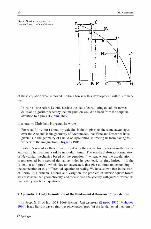
Fig. 6 Newton’s diagram forLemma 2, sect 1 of the Principia

of these equation were removed. Leibniz foresaw this development with his remarkthat

In truth no one before Leibniz has had the idea of constituting out of this new cal-culus and algorithm whereby the imagination would be freed from the perpetualattention to figures (Leibniz 1849)

In a letter to Christiann Huygens, he wrote

For what I love most about my calculus is that it gives us the same advantagesover the Ancients in the geometry of Archimedes, that Viète and Descartes havegiven us in the geometry of Euclid or Apollonios, in freeing us from having towork with the imagination (Huygens 1905)

Leibniz’s remarks offers some insight why the connection between mathematicsand reality has become a riddle in modern times. The standard abstract formulationof Newtonian mechanics based on the equation f = ma, where the acceleration ais represented by a second derivative, hides its geometric origins. Indeed, it is the“attention to figures”, which Newton advocated, that give us some understanding ofthe connection of this differential equation to reality. We have shown that in the workof Bernoulli, Hermann, Leibniz and Varignon, the problem of inverse square forceswas first visualized geometrically, and then solved analytically with finite differentialsthat satisfy algebraic equations.

7 Appendix 1. Early formulation of the fundamental theorem of the calculus

In Prop. X:11 of his 1668–1669 Geometrical Lectures (Barrow 1916; Mahoney1990), Isaac Barrow gave a rigorous geometrical proof of the fundamental theorem of

123

The early application of the calculus 295

the calculus.46 Barrow proved that the subtangent of a curve with ordinate Yx for thearea bounded by another curve yx at a corresponding value of x of the abscissa, is pro-portional to the ratio Yx/yx. In a 1693 article in the Acta Eruditorum (Leibniz 1693),Leibniz essentially took over Barrow’s geometrical proof, substituting the differentialform for the subtangent, Yxdx/dYx, to write Barrow’s result, Yxdx/dYx = aYx/yx,in the form aYx = ∫

yxdx, where a is an arbitray constant of proportionality with thedimension of length.

In an appendix to his lectures, Barrow also gave a bound for the area of a curve bythe sum of the areas of rectangles, which later Newton adopted as Lemma 2 of Sect. 1in the Principia. Barrow’s bound served as the starting point for an analytic proof of thefundamental theorem along the lines developed by Leibniz and Newton. Referring toFig. 6, which corresponds to Barrow’s diagram as it appeared in Lemma 2, let yi be theordinate of the curve at xi for i = 1−5. Then y1 = Aa, y2 = Bb, y3 = Cd, y4 = Ddand y5 = Ee, and x1 = 0,x2 = AB,x3 = AC,x4 = AD, and x5 = AE , whereAB = BC = C D = DE , i.e., the corresponding rectangles have equal differentialwidths dx = xi+1 − xi . The upper bound U for the area under the curve is

U =i=4∑

i=1

yi dx, (75)

the lower bound D is

D =i=4∑

i=2

yi dx, (76)

and the difference U − D is the area of the first rectangle

U − D = y1dx. (77)

Geometrically, this result can also be seen to be the sum of the area of the residualrectangles aI bK , bmcL , cnd M and deE D. Of course, this result applies also for asubdivision with n equal rectangles. It follows that when the magnitude of the differ-ential dx is decreased, and accordingly the number n of rectangles is increased, thedifference U − D between the upper and lower bounds to the area under the curve,which is proportional to dx, also decreases. In the limit that dx becomes vanishinglysmall, this difference becomes zero giving a proof equivalent to Archimedes methodby exhaustion that either bound approaches the area.

Hence, by taking a sufficiently large number n of rectangles, the sum of differentials

Yn =i=n∑

i=1

yi dx (78)

46 In a letter to Oldenburg meant for Leibniz, written on Oct 24, 1676, Newton formulated this theorem inthe form of an anagram that reads “given an equation involving any number of fluent quantities to find thefluxions, and conversely” (Newton 1676).

123

296 M. Nauenberg

for i = 1 to i = n, where dx = xi+1 − xi is a constant, determines the area underthe curve in the interval x = 0,x = xn to any desired accuracy.47 In turn, the sum Yi

satisfies the property that the difference

dYi = Yi+1 − Yi = yi+1dx (79)

is determined by yi+1 and the magnitude of the differential dx. Taking x as a variable,let Yx be the area bounded by the curve yx = yi , and the ordinates x1 and x. Then inthe limit that dx → 0 the ratio dYx/dx approaches the tangent of the curve Yx, andaccording to Eq. 79

dYx

dx→ yx (80)

This relation represents in algebraic form Barrow’s geometrical theorem. In Leib-niz’s suggestive notation where the summation sign

∑is replaced by the integral

sign∫

Yx =x∫

x1

yxdx (81)

In Newton’s equivalent language for the calculus, 48 the ordinate yx with x as a uni-formly increasing variable, i.e. x = 1, represents the fluxion associated with the fluentYx, and the differential relation between Yx and yx is denoted in Newton’s notationby a dot on Yx,

Yx = yx. (82)

It is surprising that Newton did not introduce a notation for the integral of yx compara-ble to Leibniz’s, Eq. 81 and instead, he referred to the fluent Yx always as the quadratureor area associated to the curve yx. He defined also the moment of any fluent Yx or curveby Yxo, where o is a small quantity corresponding to Leibniz’s differential dx. It isalso important to recognize, that Leibniz’s differential dYx = Yx+dx − Yx is the sameas Newton’s moment Yxdx only to first order in dx.49

47 Although the sum∑i=n

i=1 yi increases with increasing n without bounds, the product (∑i=n

i=1 yi )dxremains finite, because dx = (x − x1)/n decreases with increasing n in the same proportion.48 Leibniz’s rules for the differential calculus are the same ones that Newton developed for his calculus offluxions. In 1696, the Marquis De L’Hospital published Analyse des Infiniment Petits pour L’Intelligencedes Lignes Courbes, based on lectures that he had received from Bernoulli, which became the first textbookon the differential calculus in the Continent. It was translated from French to English in 1730 by E. Stoneunder the title The Method of Fluxions both Direct and Inverse. Stone changed Leibniz differential notationinto Newton’s dot notation for fluxions, e.g., dx became xdt , and he added his own description of theintegral calculus.49 The ratio dY ′/dx of Leibniz’s “characteristic triangle” with sides dx and dY ′ is equal to the tangent Yat x. Leibniz used the same symbol dY for this different definition of the differential dY ′, which for a fixedvalue of dx is equal to Newton’s definition of the moment of Y.

123

The early application of the calculus 297

While a rigorous mathematical formulation of the limit dx → 0 had to wait foranother century, in Lemma1, Sect. 1 of the Principia Newton expressed this limitconcisely under the heading of “first and ultimate ratios” as follows:

Quantities and also ratios of quantities, which in any finite time constantly tend toequality, and which before the end of that time approach so close to one anotherthat their difference is less than any given quantity, become ultimately equal.

In practice, differentials, either geometrical or algebraic, were always representedby finite albeit very small quantities. Both Newton and Leibniz recognized that forsufficiently small values of these differentials, the results obtained from approximaterelations in which the contributions of higher order differentials were neglected wouldbe accurate to any desired degree.

8 Appendix 2

Using vector notation with Cartesian components along the x, y axis and origin at thecenter of force, we give a succinct derivation of the second-order differentials ddxand ddy for the force impulse along the lines given by Hermann based on Prop. 1 inNewton’s. This derivation is contrasted with Bernoulli’s, which was given in polarcoordinates, and with by a comparable derivation based on Prop. 6.

In reference to Hermann’s diagram shown in Fig. 2, let the positions B,C and Eon the curve ABC D. be represented by the vectors �rB = �r(t), �rC = �r(t + dt), and�rD = �r(t + 2dt). Then �rE = 2�rC − �rB , and �E D = �rD − �rE is given by

�E D = �r(t + 2dt)+ �r(t)− 2�r(t + dt)) (83)

Defining the first-order differential by �dr(t) = �r(t + dt)− �r(t), and the second-orderdifferential by �ddr(t) = �dr(t + dt)− �dr(t), we find that

�E D = �ddr(t). (84)

For an attractive central inverse square force �E D = E D�r/r , where r = √x2 + y2,

E D = −(xdy − ydx)2/ar2, and we obtain

dd�r = − �rr3 (xdy − ydx)2. (85)

which corresponds to Hermann’s result, Eq. 4, for the x component of �r .In polar coordinates r, θ , one also must take into account that the reference unit

vectors �u, �v along the radial and transverse direction are not fixed in space, but satisfythe conditions d �u = �vdθ , and d �v = �udθ . Setting �r = r �u, we have

d�r = dr �u + rdθ �v, (86)

123

298 M. Nauenberg

and

dd�r = (ddr − rdθ2)�u + (rddθ + 2drdθ)�v. (87)

For a force impulse along the radial direction, ξ �u, the second-order differential com-ponent of �ddr along the transverse direction �v must vanish, leading to Kepler’s arealaw in the form

d(r2dθ) = 0. (88)

Then

ξ ∝ ddr − rdθ2 (89)

which is the form originally obtained by Leibniz and re-derived by Bernoulli. Settingξ = −2φc2, where φ is the force and c = r2dθ is a constant, we recover Bernoulli’sresult

φ = − (ddr − rdθ2)

2c2 (90)

In the diagram associated with Prop. 6, shown in Fig. 4, let �rP = �r(t), �rQ =�r(t + dt)) represent the positions Q and P on the curve, and �rR(t) = �r(t) + �v(t)dt ,the position of R, where �v(t) is the velocity at P along the tangent line R P . Hencethe change in position �RQ = �rR − �rQ , is

�RQ = −�dr(t)+ �v(t)dt. (91)

To convert this expression to differentials, we need to express the velocity vector �v(t)in terms of first-order differentials �dr(t) with the property that in the limit when Qapproaches P , this vector remains tangential to the curve at P up to third order inpowers of dt . Introducing Q′ for the position on the orbit at time t − dt , which is notshown in Newton’ diagram, where �rQ′ = �r(t − dt), this property is satisfied uniquelyby the chord �rQ − �rQ′ = �dr(t) + �dr(t − dt). Hence, we approximate �v(t) by therelation

�v(t)dt = 1

2(�dr(t)+ �dr(t − dt)), (92)

and substituting this expression for �v(t)dt in Eq. 91, we obtain

�RQ = 1

2�ddr(t) (93)

Acknowledgements I would like to thank Niccolo Guicciardini for numerous discussion and many help-ful comments and corrections of an earlier draft of this manuscript.

123

The early application of the calculus 299

Open Access This article is distributed under the terms of the Creative Commons Attribution Noncom-mercial License which permits any noncommercial use, distribution, and reproduction in any medium,provided the original author(s) and source are credited.

References

Aiton, E. J., 1954 The Inverse Problem of Central Forces. Annals of Science 20:81–99Aiton, E. J., 1962 The Celestial Mechanics of Leibniz. Annals of Science 16:65–82Aiton, E. J., 1995 The vortex theory in competition with Newtonian celestial dynamics. Planetary astronomy

from the Renaissance to the rise of astrophysics, part B, edited by R. Taton and C. Wilson (CambridgeUniversity Press) pp. 3–21

Barrow, I., 1916 The Geometrical Lectures of Isaac Barrow. Translations and notes by J. M. Child (OpenCourt, London), Quoted by N. Guicciardini in reference (Guicciardini 2009)

Bernoulli, J., 1710 Extrait de la Résponse de M. Bernoulli à M. Herman, datée de Basle le 7. Octobre 1710.Memoires de l’Academie Royale des Sciences pp. 521–533

Bernoulli, J., 1914 Die erste Integralrechnungen Ostwald Klassiker nr. 194 (Leipzig und Berlin, 1914)63–67. Archives for the History of Exact Sciences 46, 222–251

Bernoulli, J., 1999 Die Werke von Jakob Bernoulli: Bd. 5: Differentialgeometrie edited by D. Speiser, A.Weil and M. Mattmüller (Birkhaüsser)

Bernoulli, 2008 Die Werke von Johannn I und Nicolaus II Bernoulli ed. P. Radelet-de Grave (Birkhäuser)pp. 125–128

Bertoloni Meli, D., 1991 Equivalence and priority: Newton vs. Leibniz (Clarendon Press, Oxford)Boyer, C. B., 1989 A History of Mathematics (Wiley, New York)Bos, H. J. M., 1973 Differentials, Higher-Order Differentials and the Derivative in the Leibnizian Calculus.

Arch. Hist. Exact Sci. 14:1–90Brackenridge, J. B., 2003 Newton’s Easy Quadratures “Omitted for the Sake of Brevity”. Archive for

History of Exact Sciences 57, 313–336Cohen, I. B., 1999 Isaac Newton The Principia. A new translation by I. B. Cohen and Anne Whitman

assisted by Julia Budenz, and A Guide to Newton’s Principia by I. B. Cohen (University of CaliforniaPress) p. 115

Erlichson, H., 1994 The Visualization of Quadratures in the Mystery of Corollary 3 to Proposition 41 ofNewton’s Principia. Historia Mathematica 21, 148–161

Euler, L., 1736 Mechanica (St. Petersburg) Quoted in reference (Bertoloni Meli 1991) p. 214Guicciardini, N., 1999 Reading the Principia: The Debate on Newton’s Mathematical Methods for Natural

Philosophy from 187 to 1736. (Cambridge University Press, Cambridge) pp. 207–225Guicciardini, N., 2008 Isaac Newton and Johann Bernoulli on central force motion. (to be published)Guicciardini, N., 2009 Isaac Newton on Mathematical Certainty and Method (M.I.T. Press, Cambridge)Hermann, J., 1710a Extrait d’une Lettre de M. Herman à M. Bernoulli, datée de Padoüe le 12. Juillet 1710.

Memoires de l’Academie Royale des Sciences pp. 519–521Hermann, J., 1710b Metodo d’investigare l’Orbite de’ Pianeti…Giornale de’ Letterati d’ Italia, vol. 2,

447–467Huygens, C., 1673 Horologium Oscillatorium (Paris). Reproduced in Ouvres Complètes de Christiaan

Huygens, vol. 8 (Martinus Nijhoff). English translation in Richard J. Blackwell, Christiaan Huygens’sPedulum Clock (Ames 1986)

Huygens, C., 1905 Ouvres Complètes des Christiaan Huygens vol. 10 Correspondance 1691–1695 (MartinusNijhoff, The Hague) p. 227. Translation from French to English by N. Guicciardini in ref. (Guicciardini1999) p. 166

Kline, M., 1972 Mathematical Thought from Ancient to Modern Times, vol. 1 (Oxford University Press,Oxford)

Laplace, P. S., 1798 Traité de Méchanique Celeste Tome I, Premier Partie, Livre II, (Gauthier-Villars, Paris)p. 165, Ouvres Complétes de Laplace (Gauthiers-Villars, Paris, 1843) p. 181

Leibniz, G., 1693 Supplementum geometriae dimensoriare … Acta Eruditorum, 385–392. Translated intoEnglish from Leibniz, Mathematische Schriften, Abth. 2, Band I, 294–301, in A source book in mathe-matics, edited by E.D. Struik (Harvard University Press 1969) pp. 282–284

Leibniz, G. W., 1849 Mathematische Schriften vol. 5, ed. C. I. Gerhardt (Berlin) p. 393

123

300 M. Nauenberg

Leibniz, G. W., 1973 Marginalia in Newoni Prncipia Mathematica (1687) edited by E. A. Fellman (LibrariePhilosophique J Vrin, Paris)

Mahoney, M. S., 1990 Barrow’s mathematics: between ancients and moderns, in Before Newton: The lifeand times of Isaac Barrow, edited by Mordechai Feingold (Cambridge University Press, Cambridge) pp.179–249

Mazzone, S. and Roero, C. S., 1997 Jacob Hermann and the diffusion of the Leibnizian calculus in Itally(Olschki, Firenze)

Nauenberg, M., 1994 Newton’s Early Computation for DynamicsNauenberg, M., 2003 Kepler’s area law in the Principia: filling in some details in Newton’s proof of Prop-

osition 1. Historia Mathematica 30:441–456Nauenberg, M., 2005 Robert Hooke’s seminal contributions to orbital dynamics. Physics in Perspective 7,

4–34; reprinted in Robert Hooke Tercentennial Studies, edited by M. Cooper and M. Hunter (Ashgate,Cornwall, 2006) Physics in Perspective

Newton, I., 1670–1673 The Mathematical Papers of Isaac Newton vol. 3, 1670–1673, edited by D.T. White-side (Cambridge University Press) pp. 154–155

Newton, I., 1960 The correspondence of Isaac Newton vol. 3 edited by H. W. Turnbull (Cambridge Uni-versity Press) p. 297

Newton, I., 1968 The Mathematical Papers of Isaac Newton vol. 2, edited by D.T. Whiteside (CambridgeUniversit Press, Cambridge) p. 270

Newton, I., 1974 The Mathematical Papers of Isaac Newton vol. 6, 1684-1691, edited by D.T. Whiteside(Cambridge University Press, 1974) pp. 35–37

Newton, I., 1676 The correspondence of Isaac Newton, vol. 2, 1676-1687, edited by H.W. Turnbull (Cam-bridge University Press 1976)

Varignon, M., 1710 Des forces Centrales Memoires de l’Academie Royale des Sciences 533–544Wilson, C., 1994 Newton’s Orbit Problem: A Historian’s Response. The College Mathematics Journal

25:193–205

123