The Effects of Autoscaling in Cloud Computing on Product Launch∗

Amir Fazli Amin Sayedi Jeffrey D. Shulman

March 13, 2017

∗University of Washington, Foster School of Business. All authors contributed equally to this manuscript. AmirFazli (fazli@uw.edu) is a Ph.D. Student in Marketing, Amin Sayedi (aminsa@uw.edu) is an Assistant Professor ofMarketing and Jeffrey D. Shulman (jshulman@uw.edu) is the Marion B. Ingersoll Associate Professor of Marketing,all at the Michael G. Foster School of Business, University of Washington.

1

The Effects of Autoscaling in Cloud Computing on Product

Launch

Abstract

Web-based firms often rely on computational resources to serve their customers, though

rarely is the number of customers they will serve known at the time of product launch. Today,

many of these computations are run using cloud computing. A recent innovation in cloud

computing known as autoscaling allows companies to automatically scale their computational

load up or down as needed. We build a game theory model to examine how autoscaling will affect

firms’ decisions to enter a new market and the resulting equilibrium prices, profitability, and

consumer surplus. Prior to autoscaling, firms planning to launch a new product needed to set

their computational capacity before realizing their computational demands. With autoscaling,

a company can be assured of meeting demand and pay only for the demand that is realized.

Though autoscaling decreases expenditures on unneeded computational resources and therefore

should make market entry more attractive, we find this is not always the case. We highlight

strategic forces that determine the equilibrium outcome. Our model identifies the likelihood of

a firm’s success in a new market and differentiation among potential entrants in the market as

key drivers of whether autoscaling increases or decreases market entry, prices, and consumer

surplus.

1 Introduction

Consider an entrepreneur or firm deciding whether to launch a web service in a new market.

Getting started requires an investment of time and money into research, development, legal, and

other starting expenses prior to knowing whether the new product will ever succeed. Furthermore,

web and mobile-based firms rely on computational capacity to serve customers. Every interaction

a customer has with an application such as a page load, data transfer, and object viewing requires

computational resources. This is particularly relevant to companies launching a Software as a

Service (SaaS), an industry estimated at $49 billion and expected to grow to $67 billion by 2018

(Columbus 2015). For any company relying on computational resources, cloud computing allows

the company to outsource the server set-up and maintenance to a cloud provider.

1

More and more companies are adopting the cloud to handle their computational needs. Exam-

ples of companies using the cloud include big firms such as Netflix, Airbnb, Pinterest, Samsung,

Expedia, and Spotify as well as many small businesses and startups (Gaudin 2015; Bort 2015). In

fact, end user spending on cloud services in 2015 was estimated to be above $100 billion (Flood 2013)

with an expected annual growth of 44% in workloads (Ray 2013).

While cloud computing technology allows for the outsourcing of computational costs, firms who

ran their tasks in the cloud often needed to decide, and pre-commit to, their computational capacity

at the time of purchasing the cloud service. As such, due to the unpredictable nature of demand

for firms entering a new market, the pre-purchased capacity may be excessive or insufficient for the

traffic. This issue is specially important in the case of entrepreneurs launching a web startup. For

example, BeFunky, an online photo editing startup, was featured on a popular social media site three

weeks after launch and saw 30,000 visitors in three hours, crashing their servers (Nickelsburg 2016).

Such events happen regularly enough that there is a term for it: the Slashdot effect, which Klems,

Nimis, and Tai (2008) describe as occuring when a startup is featured on a popular network,

resulting in a significant increase in traffic load and causing the firm’s servers to slow down or

crash. Such a problem can be quite costly as an Aberdeen study found that “a 1-second delay in

page load time can result in a 7% loss in conversion and a 16% decrease in customer satisfaction”

(Poepsel 2008). Kissmetrics, an analytics company, reports that 1 in 4 people abandon a page

if it takes longer than 4 seconds to load (Work 2011). Though capacity can later be increased,

the missed demand can be costly. As Amazon CEO Jeff Bezos describes, startups face a serious

challenge when choosing computational capacity:1

“And you do face this issue (demand uncertainty) whenever you have a startup company.

You want to be prepared for lightning to strike because if you’re not, that generates

a big regret. If lightning strikes and you weren’t ready for it, that’s kind of hard to

live with. At the same time, you don’t want to prepare your physical infrastructure to

hubris levels either in the case that lightning doesn’t strike.”

To address this challenge, cloud providers such as Amazon, Microsoft, and Google have begun

to offer autoscaling, a feature that allows firms to scale their computational capacity up or down

1https://animoto.com/blog/news/company/amazon-com-ceo-jeff-bezos-on-animoto/, accessed September 2016.

2

automatically in real time. Using autoscaling, firms launching a new web-based service can maintain

application availability and scale their computational capacity for serving consumers without having

to make capacity pre-commitments.

For companies, autoscaling means having just the right number of servers required for meeting

the demand at any point in time, which can provide an attractive solution to handling uncertain

demand in new markets. Autoscaling is offered with no additional fees and has been celebrated

as one of the most beneficial features of cloud computing. Users of autoscaling such as AdRoll

and Netflix find that when a new customer comes on board, they can handle the additional traffic

instantly.2 As Mikko Peltola, the Operations Lead at Rovio, noted regarding the benefits of au-

toscaling, “We can scale up as the number of players go up ... so we can automatically increase

the processing power for our servers.”3 The Chief Technology Officer for Cloud at General Electric

has mentioned this feature as one of the main reasons for the company’s move to the cloud, stating

“Running inside a public cloud environment, you’re able to consume unlimited capacity as needed”

(Weaver 2015). Anecdotally, some entrepreneurs such as Animoto CEO, Brad Jefferson, who used

Amazon Web Services (AWS), see the scaling it offers as a game changer for their product launch:

“We simply could not have launched Animoto.com and our professional video rendering platform

at our current scale without massive CapEx and a lot of VC funding. The viral spike in Animoto

video creations we experienced this week would have been disastrous without AWS.”4

In this paper, we develop an analytical model to examine how the emergence of autoscaling

in cloud computing will affect web-based firms’ decisions regarding market entry and prices. In

particular, despite popular belief, we identify conditions for when autoscaling negatively affects

market entry. In other words, fewer firms will enter in certain markets due to the advent of

autoscaling. Autoscaling has several properties that make it unique from some previously explored

areas in marketing and operations. In particular, autoscaling:

• removes a capacity decision that otherwise has to be made prior to pricing;

• converts computational capacity costs from fixed costs to variable costs at the time of pricing;

• allows capacity to be set after the uncertainties regarding consumers’ level of interest and

2See https://aws.amazon.com/solutions/case-studies/adroll/3See https://aws.amazon.com/solutions/case-studies/rovio/4https://animoto.com/blog/news/company/amazon-com-ceo-jeff-bezos-on-animoto/, accessed September 2016.

3

competitors’ strategies are resolved; however, autoscaling still

• preserves the uncertainty that exists at the time of making the entry decision.

Given these properties, the effects of autoscaling on company strategies cannot be addressed by

prior research on capacity choices and demand uncertainty. In fact, our model and predictions

diverge from prior literature substantively.

We uniquely incorporate these properties of autoscaling into a game theory model in which two

horizontally differentiated firms have the option to enter a market upon incurring an entry cost.

We compare a model in which firms choose computational capacity to a model in which firms can

choose to adopt autoscaling in cloud computing. The model is constructed to address the following

research questions:

1. How does autoscaling affect firms’ profits in the new market?

2. How does autoscaling affect pricing strategies at launch?

3. How does autoscaling affect market entry decisions?

4. How does autoscaling affect consumer surplus?

We explore the roles of several important market factors in determining the answer to each of

the research questions. First, we model the ex ante likelihood of a successful product launch. As

Griffith (2014) suggests, the value that a firm brings to a new market is unknown before market

entry. In some markets, consumer needs are well known and established, therefore yielding a higher

likelihood of successfully creating a product that matches consumer needs. For other markets, the

consumer needs are less understood and there is a lower likelihood of a successful venture. We

show that the likelihood of a successful venture plays a critical role in determining how autoscaling

affects equilibrium strategies and profits.

Secondly, we model competition among market entrants. As Burke and Hussels (2013) suggest,

competition in new markets is a key factor in determining the performance of new products. In

fact, without accounting for competition, autoscaling has a strictly positive impact on the profit of

the firm introducing a new product. However, a conventional study of autoscaling for a monopoly

does not capture the strategic interactions inherent to autoscaling. By analyzing a competitive

4

game theory model, we capture these strategic effects and find autoscaling can actually decrease

the profits of competing firms.

We identify three general effects of autoscaling: First, the downside risk reducing effect of

autoscaling prevents firms from investing in excess capacity in case their product is not successful.

Second, the demand satisfaction effect of autoscaling allows firms to fully serve the demand without

facing insufficient capacity in case their product is successful. Finally, autoscaling also has a

competition intensifying effect, which can result in lower prices and profitability if multiple firms

enter the market.

In answering the first research question, we find that autoscaling can increase or decrease firms’

expected profits in the new market. We identify strategic consequences of autoscaling and the con-

ditions that lead to each possibility. In particular, when the probability of success is sufficiently low,

autoscaling increases the firms’ expected profits. However, autoscaling may also create a prisoner’s

dilemma situation where firms choose autoscaling, but autoscaling lowers their equilibrium profits.

In particular, when entry costs are sufficiently small and the probability of success is moderately

high, firms adopt autoscaling in equilibrium; however, their equilibrium profits would be higher if

autoscaling was not available. This counterintuitive result is driven by the competition intensifying

effect outweighing the demand satisfaction and downside risk reducing effects of autoscaling.

In addressing the second research question, we find that autoscaling may increase or decrease

average prices charged by competing firms. Existing economic theory would suggest that removing

the capacity decision prior to pricing would result in a shift from a Cournot game to a Bertrand

game, thereby decreasing prices (e.g., Kreps and Scheinkman 1983). However, our model shows

that when both firms enter the market, autoscaling increases the average prices set by each firm

if the probability of a successful venture is not too high. On the other hand, if the probability of

a successful venture is sufficiently high, then autoscaling decreases the average prices set by each

firm. Our model shows that the probability of success plays a critical role in the firms’ capacity

choice without autoscaling and therefore influences the magnitude of the demand satisfaction and

downside risk reducing effects of autoscaling relative to the competition intensifying effect.

With regard to the third research question, we find that autoscaling can actually decrease

market entry. Though we confirm common intuition that the likelihood of a market being served

by at least one firm is improved with autoscaling, we find that, under certain conditions, entry

5

by multiple firms will not occur because of autoscaling. The counter-intuitive result occurs due to

competition in the new market, when entry costs are moderately high and there is a high probability

that entrants will have a successful venture. In this region, the two firms anticipate autoscaling

will heighten price competition after entry, and one firm, therefore, avoids entering the market

altogether.

Finally, in addressing the fourth research question, we show that autoscaling may increase

or decrease expected consumer surplus depending on the likelihood of a successful venture and

entry costs. Given the fact that autoscaling guarantees companies have the capacity to serve

consumers in case of high demand, thereby resolving issues such as the Slashdot effect, one might

expect that consumers benefit from autoscaling. However, our model shows that when entry costs

are low enough such that both firms enter the market, autoscaling decreases expected consumer

surplus if and only if the probability of a successful venture is moderate. Intuitively, autoscaling

decreases consumer surplus in the region where firms would not have set constraining capacities

without autoscaling. In this region, the competition intensifying effect of autoscaling is weak and

autoscaling increases firms’ prices, resulting in lower surplus for consumers.

The findings of this study provide implications for various players in new markets, including

startups, cloud providers and consumers. Our analysis informs firms entering web-based markets

on how autoscaling affects competitive dynamics in pricing and entry. The results suggest that a

firm should consider not only the positive direct effect of autoscaling in reducing costs, but also

the negative strategic effect in altering the nature of competition. By evaluating the probability of

success, the cost of computational capacity, and entry costs, managers can use the findings from this

study to determine whether autoscaling increases or decreases the likelihood of monopoly power over

the new market. Our findings also inform cloud providers about how autoscaling affects not only

the number of firms using the cloud, but also the number of servers each of those firms purchases.

Our model provides insights for consumers on how autoscaling affects the prices charged in the

market, showing that for high probabilities of success, average prices decrease with autoscaling

and for lower probabilities of success they increase with autoscaling. We also find conditions for

which autoscaling will decrease or increase consumer surplus, which can be used for consumer

surplus maximizing policy design. To the best of our knowledge, this paper is the first to study

the marketing aspects of cloud computing, and how it can affect prices and market entry. With

6

the growing trend of adopting the cloud by firms, cloud computing is expected to become a major

part of any business and this provides the field of marketing with a variety of related new topics

to explore.

In addition to contributions to practice, our work contributes to economic theory regarding ca-

pacity commitments. Our benchmark model uniquely solves a capacity choice game with demand

uncertainty and horizontal differentiation between sellers. Contrary to the previous literature,

where capacity commitments lead to higher prices, we show that under demand uncertainty, capac-

ity commitments (relative to autoscaling) can intensify the competition and cause lower equilibrium

prices. We also uniquely study the effects of removing capacity commitments made under demand

uncertainty (via autoscaling) on firms’ market entry decisions.

The rest of this paper is organized in the following order. In Section 2, we review the literature

related to our research problem. In Section 3, we introduce the model. In Section 4, we present the

analysis of the model and derive the results. We conduct a series of robustness checks and extensions

to our model in Section 5. Finally, the discussion of our findings is presented in Section 6.

2 Literature Review

Academic research on cloud computing is still relatively new and most of the work done on this

topic focuses on technological issues of the cloud (e.g., Yang and Tate 2012). The few existing

business and economics studies of cloud computing have mainly offered conceptual theories and

evidence from surveys and specific cases (e.g., Leavitt 2009; Walker 2009; Gupta, Seetharaman,

and Raj 2013). Sultan (2011) suggests that cloud computing can benefit small companies due to

its flexible cost structure and scalability. Regarding the ability to autoscale, Armbrust et al. (2009)

suggest that elasticity in the cloud shifts the risk of misestimating the workload from the user to the

cloud provider. Regarding market entry, Marston, Li, Bandyopadhyay, Zhang, and Ghalsasi (2011)

conceptually argue that cloud computing can reduce costs of entry and decrease time to market by

eliminating upfront investments. Our paper is the first to model autoscaling in the cloud and show

how its effects on market entry are not always positive, and depend on market characteristics.

In addition to cloud computing, our research is related to a number of topics in the literature.

In particular, previous research shows uncertainty in demand plays an important role in capacity

7

and production decisions. Desai, Koenigsberg, and Purohit (2007) find the optimal inventory with

demand uncertainty as a function of a product’s durability. Ferguson and Koenigsberg (2007)

examine how a firm should sell its deteriorating perishable inventory and compare this option to

discarding the previously unsold stock. Desai, Koenigsberg, and Purohit (2010) find a strategic

reason for retailers to carry inventory larger than the expected sales in both high and low demand

states. Biyalogorsky and Koenigsberg (2014) consider product introductions by a monopolist facing

uncertainty about consumer valuations and find whether the firm offers multiple products simulta-

neously or sequentially.

Our research is particularly related to the literature considering optimal timing of production

under demand uncertainty. Van Mieghem and Dada (1999) consider a monopoly firm making three

decisions: capacity investment, production quantity, and price. They study the effect of postponing

the two latter decisions. Anupindi and Jiang (2008) study the strategic effects of competition in a

model with flexible production timing. Anand and Girotra (2007) allow firms to postpone product

differentiation by customizing products after more demand information is revealed. Goyal and

Netessine (2007) allow firms to choose between product-flexible or product-dedicated technologies

and invest in capacity before demand uncertainty is resolved, while postponing production decisions

until demand is revealed. These previous studies on postponing production separate the capacity

decision and the production decision: The capacity decision is assumed to occur before demand is

revealed and it is the production decision that can be postponed. With cloud computing, there

is zero production cost after the firm chooses its computational capacity and autoscaling allows

both capacity and production to simultaneously match with demand. In the mentioned papers

on timing of production, capacity constraints are set before demand realization and they influence

how many customers are served, regardless of the timing of production. However, autoscaling

uniquely eliminates the effect of capacity constraints under demand uncertainty, resulting in findings

different from the production postponement literature. For instance, Anupindi and Jiang (2008)

find production postponement increases capacity investment and profitability, whereas we find

when autoscaling may decrease equilibrium computational expenditures and when it may decrease

profitability.

Che, Narasimhan, and Padmanabhan (2010) allow for eliminating the capacity decision under

demand uncertainty by considering a firm’s decision between adopting a make-to-stock system, a

8

backorder system, or a combination of both. However, a firm’s decision of using autoscaling is con-

ceptually different from the decision between make-to-stock and backorder production. Backorder

production delays the time at which customers are served compared to a make-to-stock production,

resulting in factors such as time-sensitivity of customers and firms determining the outcome of the

model. With autoscaling, on the other hand, firms avoid capacity decision under demand uncer-

tainty while satisfying the demand at the exact same time as they would have with pre-purchased

capacity. Che, Narasimhan, and Padmanabhan (2010) find it is optimal for firms to use a combi-

nation of make-to-stock and backorder production. However, our model shows using autoscaling

and purchasing fixed capacity simultaneously is not an optimal strategy for firms using the cloud.

Our examination of how cloud computing with autoscaling affects a firm’s entry decision also

relates to the literature on market entry. A body of literature looks at the timing of entry and how

an incumbent can deter entry (e.g., Spence 1977; Joshi, Reibstein, and Zhang 2009; Milgrom and

Roberts 1982; and Ofek and Turut 2013). Narasimhan and Zhang (2000) consider firms’ decisions

on order of entry into markets with demand uncertainty. They study how market entry from the

first mover can unfold market information and resolve demand uncertainty for the second entrant.

In contrast, our model examines simultaneous entry decisions by firms, such that both firms face

equal demand uncertainty when making entry decisions. Our model adds to entry literature by

jointly considering both entry and capacity decisions, such that each firm’s decision to enter depends

on the expected future capacity of both firms and whether this capacity will be chosen ex ante or

autoscaled to demand.

We compare autoscaling with cases where firms commit to their computational capacity before

pricing and realizing demand. This relates to other papers examining capacity commitments. Kreps

and Scheinkman (1983) find that a Bertrand pricing game becomes a Cournot game when capacity is

chosen prior to pricing. Reynolds and Wilson (2000) extend this model to include uncertainty about

market size and find there is no symmetric, pure-strategy equilibrium capacity choice when there is

significant demand variation. Nasser and Turcic (2015) find symmetric horizontally differentiated

firms use asymmetric strategies on whether to commit to capacity or not. This is consistent with

our findings. However, since they do not allow for demand uncertainty, capacity commitments

always alleviate competition in their model, whereas, in ours, capacity commitments sometimes

intensify competition. Furthermore, at least one firm commits to capacity in any equilibrium

9

in their model, whereas, in our model, both firms may use autoscaling. Swinney, Cachon, and

Netessine (2011) examine the optimal timing of capacity investment in a model in which market

price is given by a demand curve and firms can choose to set capacity early at one marginal cost of

capacity or after demand is realized at a different cost of capacity. Van Mieghem and Dada (1999)

allow firms to choose the time of their pricing decisions and find that postponing pricing until

after demand is realized makes the capacity decision less sensitive to demand uncertainty. Our

research expands this literature by considering demand uncertainty and market entry decisions

in a horizontally differentiated market with and without capacity commitments. In contrast to

the previous literature where capacity commitments always alleviate competition, we show that,

depending on the level of demand uncertainty, capacity commitments may indeed intensify the

competition. Furthermore, in our model, firms decide whether to adopt autoscaling or to pre-

commit to capacity; we find that firms do not always follow symmetric strategies in regards to

adoption of autoscaling. Finally, we uniquely explore how entry decisions are affected by existence

of capacity commitments under demand uncertainty.

Autoscaling in cloud computing also has the effect of converting up-front capacity costs to

variable costs that change with demand. Prior research examining the effect of converting fixed to

variable costs via outsourcing (e.g., Shy and Stenbacka 2003; Buehler and Haucap 2006; Chen and

Wu 2013) have found that prices and profitability rise with this conversion. However, these models

do not allow for demand uncertainty. In our model, the decision between up-front investments in

capacity and opting for variable cost of capacity through autoscaling is dependent on the level of

demand uncertainty in the market. Also, relative to these outsourcing models, up-front capacity

cost is endogenous in our model since firms can choose their capacity. Accounting for demand

uncertainty and endogenous upfront costs provides novel insights on fixed versus variable capacity

costs. In contrast to prior outsourcing literature, we show average prices can fall when cloud

computing with autoscaling is used even in conditions for which entry is unaffected.

In summary, our paper uniquely compares market entry, pricing, and profitability between

computing resources requiring capacity pre-commitments and cloud computing with autoscaling.

The advent of cloud computing with autoscaling has several properties: 1. Autoscaling allows for

capacity decisions to be made after the demand uncertainty is resolved. 2. Autoscaling converts

the fixed cost of computational resources that is sunk prior to the firms’ pricing decision into

10

variable costs that are directly affected by the pricing decision. 3. Autoscaling makes it such

that capacity and pricing decisions are made simultaneously rather than sequentially. However,

autoscaling does not affect the level of uncertainty at the time a firm makes its entry decision.

Though previous research has separately examined demand uncertainty, the timing of capacity

and pricing decisions, or the conversion of fixed costs to variable costs, our paper is unique in

its comprehensive examination of the effect of autoscaling. In particular, our paper is the first

to solve for entry, capacity and pricing decisions in a model of horizontally differentiated firms

with demand uncertainty and to compare this equilibrium to the entry and pricing decisions of

horizontally differentiated firms who make entry decisions with demand uncertainty but whose

capacity can autoscale to the demand realized upon setting prices.

3 Model

We consider two symmetric firms who could potentially enter a particular web or mobile application

market. To enter the market, the firms would incur a fixed entry cost, F . This cost includes starting

expenses such as legal, research and development, and human capital investments. To model post-

entry competition, we adopt a discrete horizontal differentiation model (e.g., Narasimhan 1988;

Iyer, Soberman, and Villas-Boas 2005; Zhang and Katona 2012; Zhou, Mela, and Amaldoss 2015)

with three consumer segments, each consumer demanding at most one unit of the product.5 Upon

entry, each Firm i will find a segment of consumers, Segment i with i ∈ {1, 2}, who will buy

from Firm i if and only if the price pi is below their reservation value vi and who will derive zero

value from the competitor’s product. This captures the reality that consumers vary in their taste

preferences regardless of firm entry and that firms have idiosyncratic differences that will allow

them to serve these tastes differently from each other upon successful entry. The size of each

Segment i is given by α < 1/2 for i ∈ {1, 2}. The remaining 1−2α consumers are in Segment 3 and

are indifferent between firms, prefering to buy from the firm with the lowest price. The parameter

α can be interpreted as the extent to which consumers vary in their taste preferences. Note that α

also represents the level of competition in the market; for α = 12 , Segment 3 disappears, each firm

5We should note that the Hotelling model also leads to mixed strategy equilibrium in the pricing subgame whenthere are capacity constraints. The reason that we use the discrete model in Narasimhan (1988) is that, unlike theHotelling model, it gives us ordinary differential equations when we add capacity decisions to that model.

11

gets a local monopoly, and there is no competition between the firms. As α becomes smaller, the

segment of consumers for which both firms compete grows and competition intensifies.

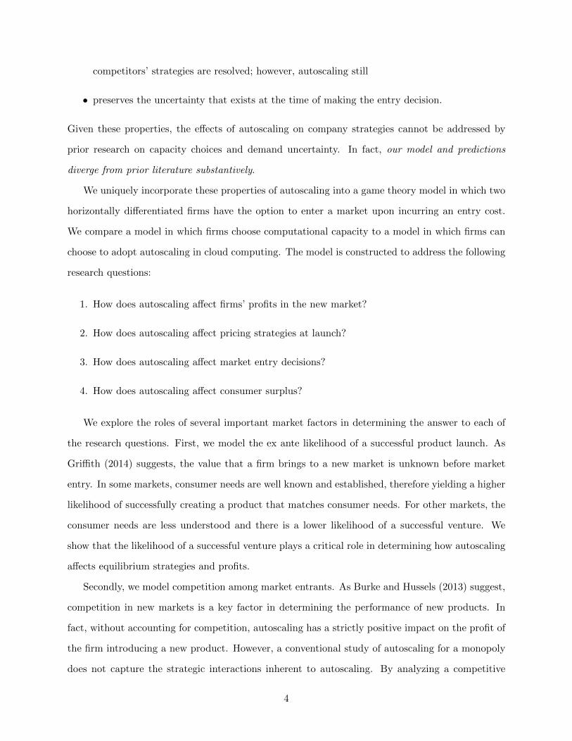
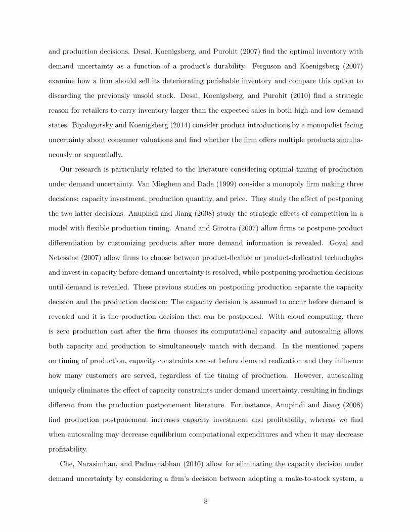
In the absence of autoscaling, the timing of the game is as follows:

Stage 1: Firms simultaneously decide whether or not to enter the market and thereby incur the

cost F . We allow for uncertainty in whether a firm will find the venture successful in terms of

whether vi is high or low. We assume the ex ante probability of a firm finding success in this

market is γ, which is common knowledge. In other words, if Firm i enters the market, vi is an i.i.d.

draw from a binary distribution in which vi = 1 with probability γ and vi = 0 with probability

1−γ. This assumption reflects the idea that the value provided to customers is unclear for potential

entrants. As Lilien and Yoon (1990) argue, the fit between market requirements and the offering of

the new entrant is highly unpredictable and is critical to the success of the entrant. In a survey of

101 startups, it was reported that the number one reason for the failure of a startup is the lack of

market need for the offered product (Griffith 2014), suggesting that the value created for customers

in a new market is unknown to many firms before entry. In an extension, we allow the low value

condition to be vi = vL > 0 and verify our results are robust to the assumption.

To remark on the structure of demand and uncertainty, notice that our model set up has several

desirable properties. In particular, it allows a firm to be uncertain about the size of the potential

market and the effect of its price on realized demand: the firm may find itself a monopolist, the firm

may find itself with very low demand (normalized to zero), or the firm may find itself competing

head-to-head. Moreover, a firm’s price relative to its competitor’s is not the only source of de-

mand uncertainty. Though one can explore alternative model specifications to capture these same

properties, the current specification allows for tractability while uncovering a novel mechanism.

Stage 2: Firms that enter simultaneously choose computational capacity ki and incur a computa-

tional capacity cost cki.

Stage 3: The reservation value for each Firm i, vi, becomes common knowledge and each firm in

the market simultaneously chooses pi to maximize profit.

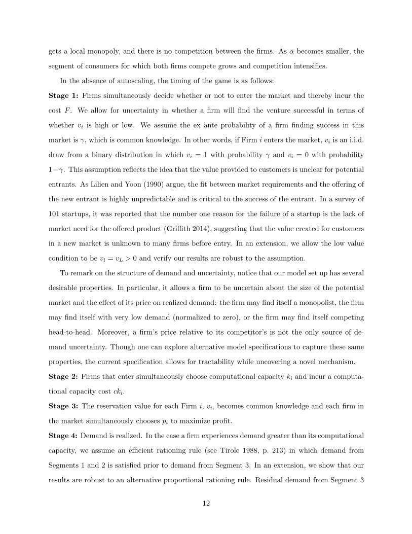
Stage 4: Demand is realized. In the case a firm experiences demand greater than its computational

capacity, we assume an efficient rationing rule (see Tirole 1988, p. 213) in which demand from

Segments 1 and 2 is satisfied prior to demand from Segment 3. In an extension, we show that our

results are robust to an alternative proportional rationing rule. Residual demand from Segment 3

12

Stage 2 Firms simultaneously choose capacity, ki.

Stage 3 Firms learn vi and

simultaneously choose price, pi.

Stage 1 Firms simultaneously decide

whether to enter.

Stage 4 Demand is realized and allocated according to an efficient rationing rule.

Figure 1: Sequence of events with no autoscaling

is allocated to the competing firm, provided it has available capacity.

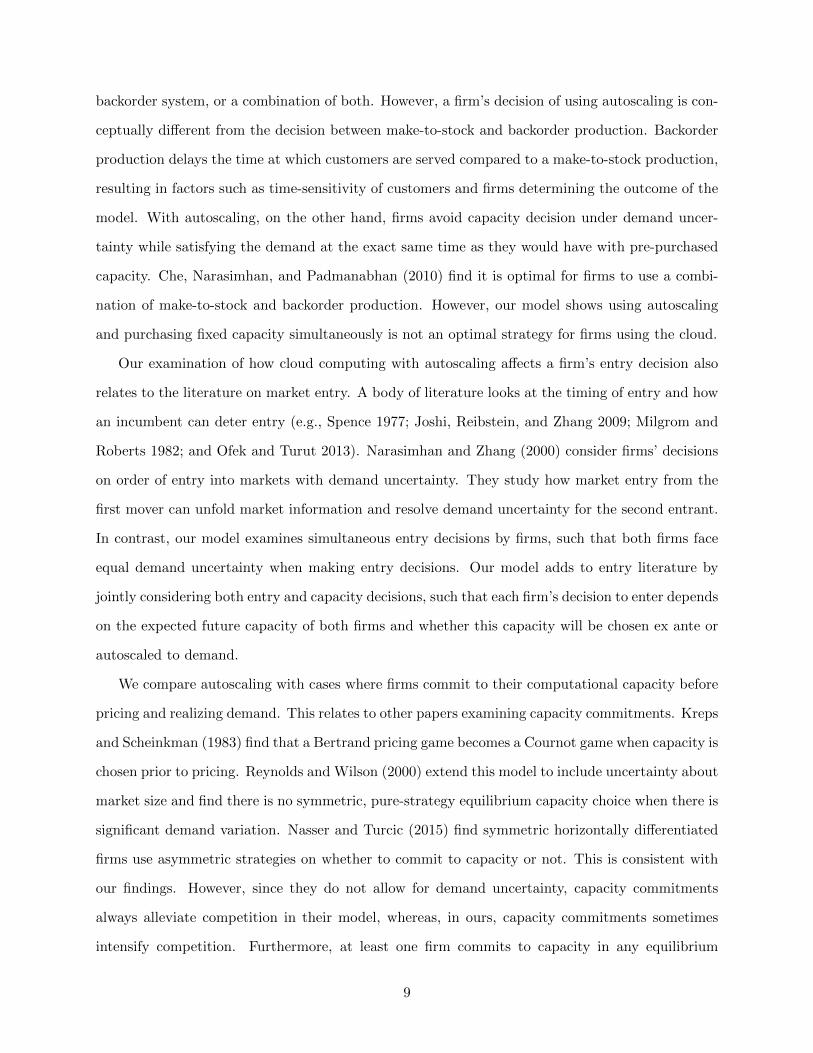
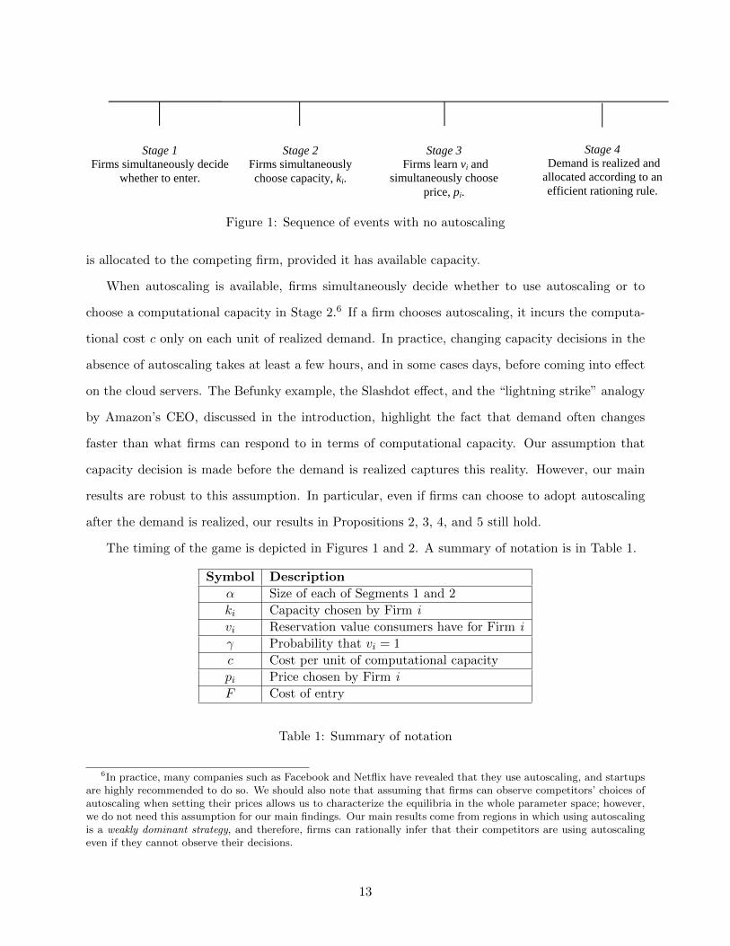
When autoscaling is available, firms simultaneously decide whether to use autoscaling or to

choose a computational capacity in Stage 2.6 If a firm chooses autoscaling, it incurs the computa-

tional cost c only on each unit of realized demand. In practice, changing capacity decisions in the

absence of autoscaling takes at least a few hours, and in some cases days, before coming into effect

on the cloud servers. The Befunky example, the Slashdot effect, and the “lightning strike” analogy

by Amazon’s CEO, discussed in the introduction, highlight the fact that demand often changes

faster than what firms can respond to in terms of computational capacity. Our assumption that

capacity decision is made before the demand is realized captures this reality. However, our main

results are robust to this assumption. In particular, even if firms can choose to adopt autoscaling

after the demand is realized, our results in Propositions 2, 3, 4, and 5 still hold.

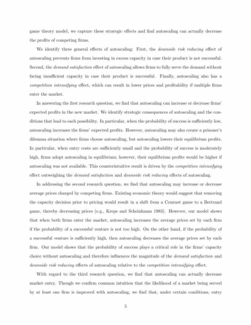
The timing of the game is depicted in Figures 1 and 2. A summary of notation is in Table 1.

Symbol Description

α Size of each of Segments 1 and 2

ki Capacity chosen by Firm i

vi Reservation value consumers have for Firm i

γ Probability that vi = 1

c Cost per unit of computational capacity

pi Price chosen by Firm i

F Cost of entry

Table 1: Summary of notation

6In practice, many companies such as Facebook and Netflix have revealed that they use autoscaling, and startupsare highly recommended to do so. We should also note that assuming that firms can observe competitors’ choices ofautoscaling when setting their prices allows us to characterize the equilibria in the whole parameter space; however,we do not need this assumption for our main findings. Our main results come from regions in which using autoscalingis a weakly dominant strategy, and therefore, firms can rationally infer that their competitors are using autoscalingeven if they cannot observe their decisions.

13

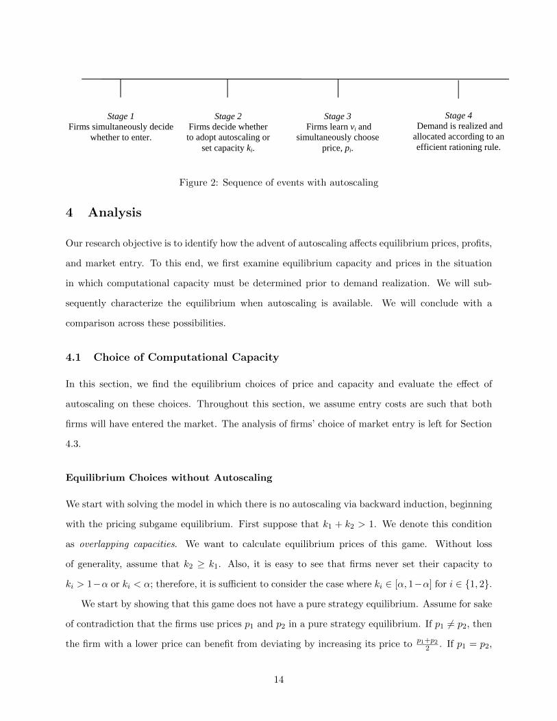
Stage 2 Firms decide whether to adopt autoscaling or

set capacity ki.

Stage 3 Firms learn vi and

simultaneously choose price, pi.

Stage 1 Firms simultaneously decide

whether to enter.

Stage 4 Demand is realized and allocated according to an efficient rationing rule.

Figure 2: Sequence of events with autoscaling

4 Analysis

Our research objective is to identify how the advent of autoscaling affects equilibrium prices, profits,

and market entry. To this end, we first examine equilibrium capacity and prices in the situation

in which computational capacity must be determined prior to demand realization. We will sub-

sequently characterize the equilibrium when autoscaling is available. We will conclude with a

comparison across these possibilities.

4.1 Choice of Computational Capacity

In this section, we find the equilibrium choices of price and capacity and evaluate the effect of

autoscaling on these choices. Throughout this section, we assume entry costs are such that both

firms will have entered the market. The analysis of firms’ choice of market entry is left for Section

4.3.

Equilibrium Choices without Autoscaling

We start with solving the model in which there is no autoscaling via backward induction, beginning

with the pricing subgame equilibrium. First suppose that k1 + k2 > 1. We denote this condition

as overlapping capacities. We want to calculate equilibrium prices of this game. Without loss

of generality, assume that k2 ≥ k1. Also, it is easy to see that firms never set their capacity to

ki > 1−α or ki < α; therefore, it is sufficient to consider the case where ki ∈ [α, 1−α] for i ∈ {1, 2}.

We start by showing that this game does not have a pure strategy equilibrium. Assume for sake

of contradiction that the firms use prices p1 and p2 in a pure strategy equilibrium. If p1 6= p2, then

the firm with a lower price can benefit from deviating by increasing its price to p1+p22 . If p1 = p2,

14

then Firm 2 can benefit from deviating by decreasing its price to p2 − ε, for sufficiently small ε, to

acquire more consumers from Segment 3. Therefore, a pure strategy equilibrium cannot exist.

Next, we find a mixed strategy equilibrium for this game. Mixed strategies can be interpreted

as sales or promotions and are common in the marketing literature (e.g., Chen and Iyer 2002, Iyer,

Soberman, and Villas-Boas 2005, Zhang and Katona 2012). Provided k1 ≤ 1−α, Firm 2 can choose

to attack with a price that clears its capacity or retreat with a price equal to 1 that harvests the

value from the 1− k1 consumers that Firm 1 cannot serve due to its capacity constraint. Let z be

the price at which Firm 2 is indifferent between attacking to sell to k2 consumers at price z and

retreating to sell to 1− k1 consumers at price 1. We have z = 1−k1k2

. Figures 3 and 4 demonstrate

the different appeals of these two pricing strategies. The choice between retreating and attacking

for each firm depends on the choice of the other firm. If Firm 1’s price is high, it becomes easier for

Firm 2 to attract the consumer segment that is in both firms’ reach resulting in Firm 2 choosing to

attack. On the other hand, if Firm 1’s price is low, Firm 2 would prefer to retreat than to compete

with Firm 1 over the overlapping consumers. In the equilibrium that we find, both firms use a

mixed strategy with prices ranging from z to 1. Suppose that Fi(.) is the cumulative distribution

function of price set by Firm i and Fj(.) is the cumulative distribution function of price set by

competing firm j.7 The profit of Firm i earned by setting price x, excluding the sunk cost of

capacity, is

πi(x) = Fj(x)(1− kj)x+ (1− Fj(x))kix.

Using equilibrium conditions, we know that the derivative of this function must be zero for x ∈ (z, 1).

Therefore, we have

−x(ki + kj − 1)F ′j(x)− Fj(x)(ki + kj − 1) + ki = 0.

The solution to this differential equation is

Fj(x) =ki

ki + kj − 1+Cjx

7We are implicitly assuming that Fi and Fj are piecewise differentiable. The game could have other mixed strategyequilibria where cumulative distribution functions of prices are not differentiable. We cannot find those equilibriausing this method.

15

where constant Cj is determined by the boundary conditions. As for the boundary conditions, we

use F1(1) = 1. Therefore, we get

F1(x) =

0 if x < z

(k1−1)+k2xx(k1+k2−1) if z ≤ x < 1

1 if x ≥ 1

(1)

This implies that Firm 1 mixes on prices between z and 1 such that Firm 2 is indifferent between

using any two prices in this range. Furthermore, given F1(.), Firm 2 strictly prefers any price in

[z, 1] to any price outside this interval. To have an equilibrium, the strategy of Firm 2 should

be such that Firm 1’s strategy is not suboptimal. In other words, Firm 1 should be indifferent

between any two prices in [z, 1], and should weakly prefer any price in [z, 1] to any price outside

this interval. Therefore, we have to use the boundary condition F2(z) = 0 to make sure that (1)

Firm 1’s indifference condition is satisfied in [z, 1], and (2) Firm 2 does not set the price to lower

than z, as we already know from F1(.) that such prices are suboptimal for Firm 2. As such, we get

F2(x) =

0 if x < z

k1((k1−1)+k2x)k2x(k1+k2−1) if z ≤ x < 1

1 if x ≥ 1

(2)

Note that F2(x) is discontinuous at x = 1, and jumps from k1k2

to 1. This implies that Firm 2 uses

price 1 with probability 1− k1k2

. In other words, f2(1) = (1− k1k2

)δ(0), where f2(.) is the probability

density function for price of Firm 2 and δ(.) is Dirac delta function.8 9

Given Fi(.), we can calculate the expected profit of each firm in this mixed strategy equilibrium.

Excluding the sunk cost of capacity, we have

π1 =(1− k1)k1

k2and π2 = (1− k1).

8See Hassani (2009), pp 139-170.9One might wonder if the probability density 1 − k1

k2allocated to price 1 by Firm 2 could be instead allocated

to price z. The answer is that it cannot. While such strategy would still keep Firm 1 indifferent between any twoprices in [z, 1], it would make price z− ε (for sufficiently small ε) a strictly better strategy for Firm 1, which violatesequilibrium conditions.

16

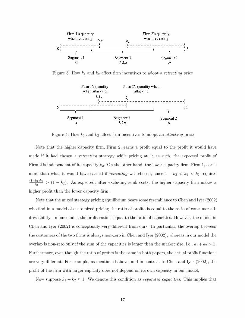
Figure 3: How k1 and k2 affect firm incentives to adopt a retreating price

Figure 4: How k1 and k2 affect firm incentives to adopt an attacking price

Note that the higher capacity firm, Firm 2, earns a profit equal to the profit it would have

made if it had chosen a retreating strategy while pricing at 1; as such, the expected profit of

Firm 2 is independent of its capacity k2. On the other hand, the lower capacity firm, Firm 1, earns

more than what it would have earned if retreating was chosen, since 1 − k2 < k1 < k2 requires

(1−k1)k1k2

> (1 − k2). As expected, after excluding sunk costs, the higher capacity firm makes a

higher profit than the lower capacity firm.

Note that the mixed strategy pricing equilibrium bears some resemblance to Chen and Iyer (2002)

who find in a model of customized pricing the ratio of profits is equal to the ratio of consumer ad-

dressability. In our model, the profit ratio is equal to the ratio of capacities. However, the model in

Chen and Iyer (2002) is conceptually very different from ours. In particular, the overlap between

the customers of the two firms is always non-zero in Chen and Iyer (2002), whereas in our model the

overlap is non-zero only if the sum of the capacities is larger than the market size, i.e., k1 + k2 > 1.

Furthermore, even though the ratio of profits is the same in both papers, the actual profit functions

are very different. For example, as mentioned above, and in contrast to Chen and Iyer (2002), the

profit of the firm with larger capacity does not depend on its own capacity in our model.

Now suppose k1 + k2 ≤ 1. We denote this condition as separated capacities. This implies that

17

each firm that enters the market can sell to its capacity without directly competing with the other

firm for consumers in Segment 3. As such, each firm that successfully enters the market can charge

pi = 1 and sell ki units for profit (1− c)ki. Increasing the price will result in zero sales and profit,

decreasing the price will still sell ki units but at lower revenue.

Next consider the capacity subgame equilibrium. The capacity decision is made in anticipation

of the possible combinations of values for v1 and v2. If both firms find success (i.e., v1 = v2 = 1),

then the profit depends on how ki and kj relate to each other and relate to α. The expected profit

for Firm i depends on its capacity relative to the capacity of competing Firm j and can be written

as follows for ki ∈ [α, 1− α]:

E(πi) =

γki − cki if ki + kj ≤ 1

γ(1− γ)ki + γ2( (1−ki)kikj)− cki if 1− kj < ki < kj

γ(1− γ)ki + γ2(1− kj)− cki if 1− ki < kj ≤ ki

where index j indicates the other firm. The equilibrium capacity choices are summarized in the

following proposition.

Proposition 1 Suppose both firms enter the market initially. The equilibrium capacity choices

depend on γ as follows:

• If there is a low probability of a successful venture (i.e., γ < c), then both firms choose ki = 0

and earn zero profit.

• If there is a moderate probability of a successful venture (i.e., γ(1 − γ) > c), then capacities

overlap such that one firm sets k = 1−α and the other firm sets k = k∗, where α < k∗ ≤ 1−α

is defined in the appendix.

• If there is a high probability of a successful venture (i.e., γ > c and γ(1 − γ) < c), then

capacities do not overlap and the unique symmetric equilibrium is k1 = k2 = 1/2.

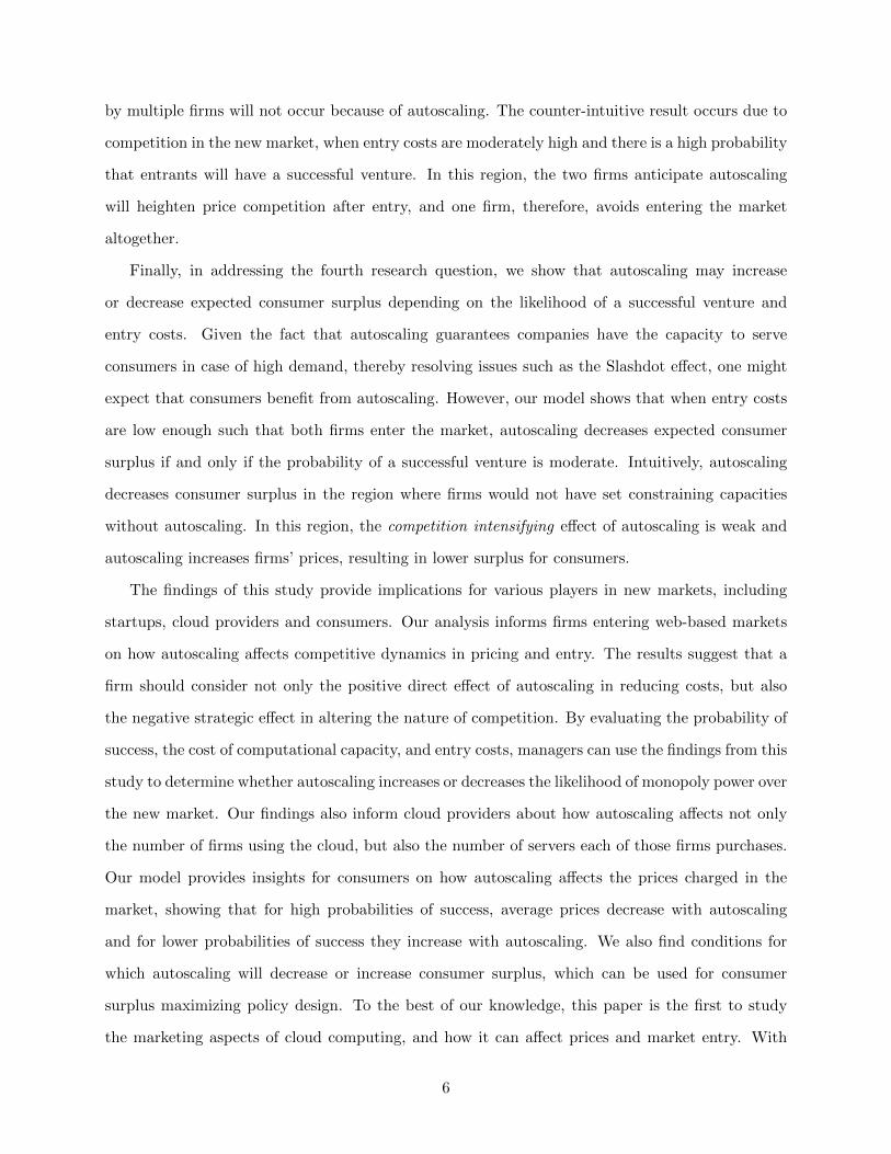
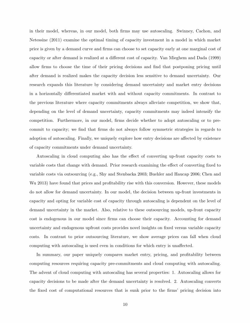
The results of Proposition 1 are depicted in Figure 5. Region 2 represents overlapping capacities

such that k1 + k2 > 1. Region 3 represents separated capacities such that k1 + k2 = 1 and in the

18

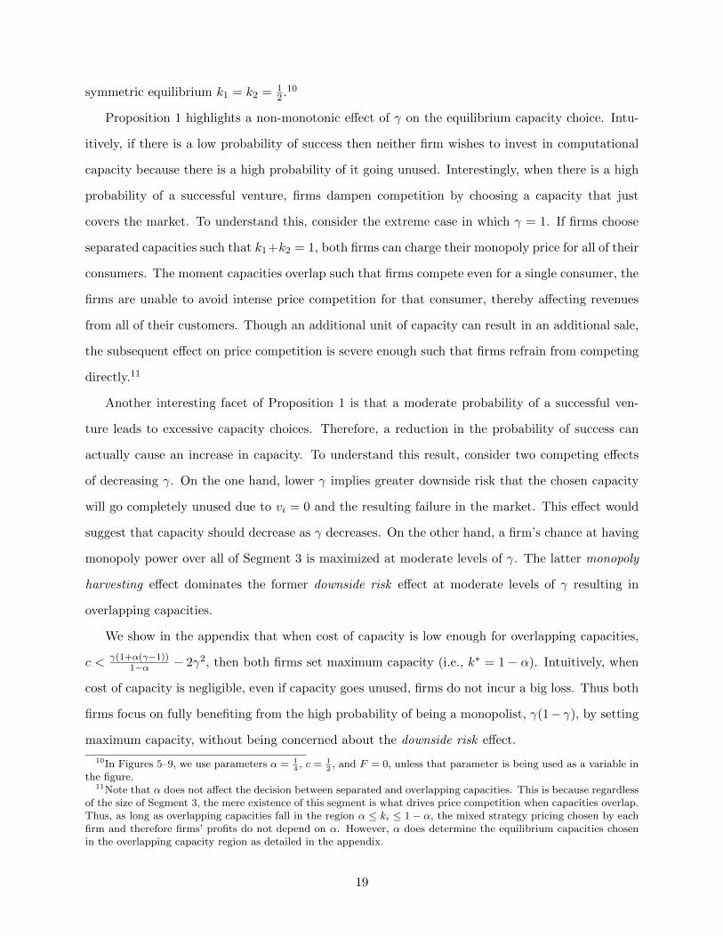
symmetric equilibrium k1 = k2 = 12 .10

Proposition 1 highlights a non-monotonic effect of γ on the equilibrium capacity choice. Intu-

itively, if there is a low probability of success then neither firm wishes to invest in computational

capacity because there is a high probability of it going unused. Interestingly, when there is a high

probability of a successful venture, firms dampen competition by choosing a capacity that just

covers the market. To understand this, consider the extreme case in which γ = 1. If firms choose

separated capacities such that k1+k2 = 1, both firms can charge their monopoly price for all of their

consumers. The moment capacities overlap such that firms compete even for a single consumer, the

firms are unable to avoid intense price competition for that consumer, thereby affecting revenues

from all of their customers. Though an additional unit of capacity can result in an additional sale,

the subsequent effect on price competition is severe enough such that firms refrain from competing

directly.11

Another interesting facet of Proposition 1 is that a moderate probability of a successful ven-

ture leads to excessive capacity choices. Therefore, a reduction in the probability of success can

actually cause an increase in capacity. To understand this result, consider two competing effects

of decreasing γ. On the one hand, lower γ implies greater downside risk that the chosen capacity

will go completely unused due to vi = 0 and the resulting failure in the market. This effect would

suggest that capacity should decrease as γ decreases. On the other hand, a firm’s chance at having

monopoly power over all of Segment 3 is maximized at moderate levels of γ. The latter monopoly

harvesting effect dominates the former downside risk effect at moderate levels of γ resulting in

overlapping capacities.

We show in the appendix that when cost of capacity is low enough for overlapping capacities,

c < γ(1+α(γ−1))1−α − 2γ2, then both firms set maximum capacity (i.e., k∗ = 1− α). Intuitively, when

cost of capacity is negligible, even if capacity goes unused, firms do not incur a big loss. Thus both

firms focus on fully benefiting from the high probability of being a monopolist, γ(1− γ), by setting

maximum capacity, without being concerned about the downside risk effect.

10In Figures 5–9, we use parameters α = 14, c = 1

2, and F = 0, unless that parameter is being used as a variable in

the figure.11Note that α does not affect the decision between separated and overlapping capacities. This is because regardless

of the size of Segment 3, the mere existence of this segment is what drives price competition when capacities overlap.Thus, as long as overlapping capacities fall in the region α ≤ ki ≤ 1 − α, the mixed strategy pricing chosen by eachfirm and therefore firms’ profits do not depend on α. However, α does determine the equilibrium capacities chosenin the overlapping capacity region as detailed in the appendix.

19

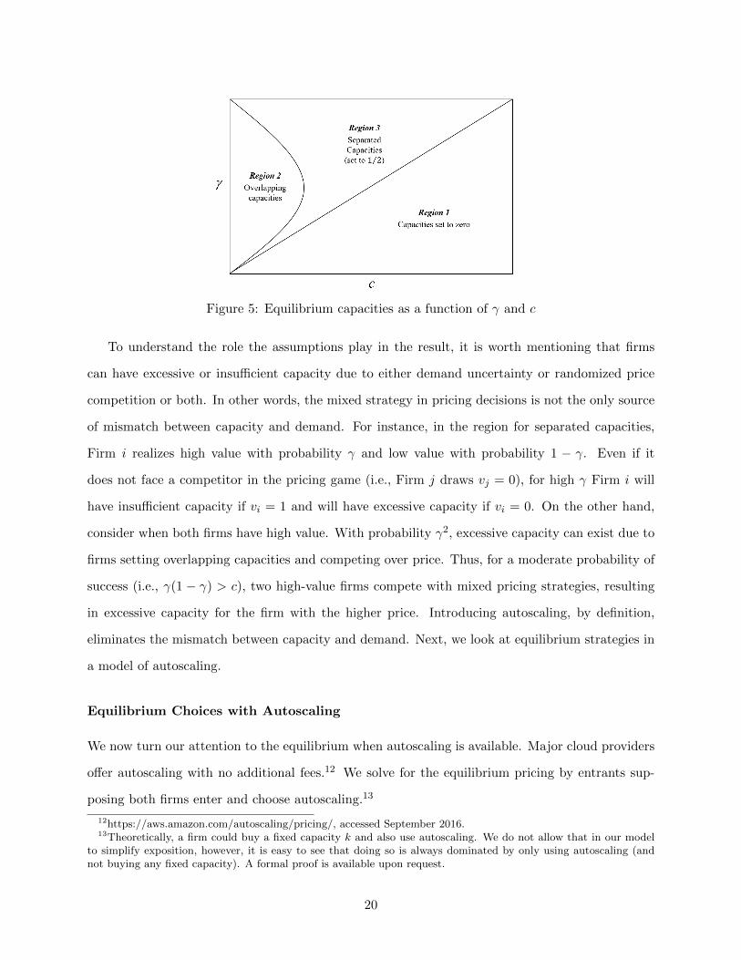
Figure 5: Equilibrium capacities as a function of γ and c

To understand the role the assumptions play in the result, it is worth mentioning that firms

can have excessive or insufficient capacity due to either demand uncertainty or randomized price

competition or both. In other words, the mixed strategy in pricing decisions is not the only source

of mismatch between capacity and demand. For instance, in the region for separated capacities,

Firm i realizes high value with probability γ and low value with probability 1 − γ. Even if it

does not face a competitor in the pricing game (i.e., Firm j draws vj = 0), for high γ Firm i will

have insufficient capacity if vi = 1 and will have excessive capacity if vi = 0. On the other hand,

consider when both firms have high value. With probability γ2, excessive capacity can exist due to

firms setting overlapping capacities and competing over price. Thus, for a moderate probability of

success (i.e., γ(1 − γ) > c), two high-value firms compete with mixed pricing strategies, resulting

in excessive capacity for the firm with the higher price. Introducing autoscaling, by definition,

eliminates the mismatch between capacity and demand. Next, we look at equilibrium strategies in

a model of autoscaling.

Equilibrium Choices with Autoscaling

We now turn our attention to the equilibrium when autoscaling is available. Major cloud providers

offer autoscaling with no additional fees.12 We solve for the equilibrium pricing by entrants sup-

posing both firms enter and choose autoscaling.13

12https://aws.amazon.com/autoscaling/pricing/, accessed September 2016.13Theoretically, a firm could buy a fixed capacity k and also use autoscaling. We do not allow that in our model

to simplify exposition, however, it is easy to see that doing so is always dominated by only using autoscaling (andnot buying any fixed capacity). A formal proof is available upon request.

20

With probability γ2, we have v1 = v2 = 1, and it is straightforward to show there is no pure

strategy pricing equilibrium; instead the pricing subgame leads to a mixed strategy equilibrium

where the prices of both firms range between z′ and 1. Similar to our analysis of mixed strategy

equilibrium without autoscaling, z′ is the price for which each firm is indifferent between attacking,

resulting in a profit of (z′ − c)(1− α), and retreating, resulting in a profit of α(1− c). This results

in z′ = α(1−c)1−α + c.

Supposing that Gi(.) is the cumulative distribution function for the price of Firm i, the profit

of Firm i when setting price x, is

πi(x) = αGj(x)(x− c) + (1−Gj(x))(1− α)(x− c)

Setting the derivative of this function equal to zero for x ∈ (z′, 1) and using the boundary conditions

G(z′) = 0 or G(1) = 1, we find

Gj(x) =

0 if x < z′

(1−α)(x−c)−α(1−c)(1−2α)(x−c) if z′ ≤ x ≤ 1

1 if x > 1

which results in the profit α(1− c) for each firm.

With probability γ(1 − γ), v1 = 1 and v2 = 0, giving Firm 1 monopoly power over all of

Segment 3 and profit of (1 − c)(1 − α). Thus, the expected profit of each firm when both use

autoscaling is (1− c)(γ2α+ γ(1− γ)(1− α)). Though we allow for firms to choose to set capacity

(rather than adopt autoscaling) even when autoscaling is available, we show in the Appendix that

there exists a c such that both firms will choose autoscaling in equilibrium if c ≥ c. In the paper,

we focus on both firms choosing autoscaling (i.e., c ≥ c), but show in the Appendix that our results

also hold for c < c, which results in only one firm choosing autoscaling.

Next, we study the effect of autoscaling on firms using the cloud and find how average prices

change with the introduction of autoscaling.

21

4.2 Effect of Autoscaling on Firms’ Prices

Given the firms’ equilibrium strategies, we can examine how autoscaling will affect equilibrium

prices in the event that entry costs are low enough such that both firms enter.

Proposition 2 Suppose entry costs are such that both firms enter the market with or without

autoscaling. The effect of autoscaling on average prices depends on γ as follows:

• In the region for separated capacities (i.e., γ > c and γ(1− γ) < c), autoscaling decreases the

average price set by each firm.

• In the region for overlapping capacities (i.e., γ(1− γ) > c), autoscaling increases the average

price set by each firm for low enough cost of capacity (i.e., c < γ(1+α(γ−1))1−α − 2γ2).

Proposition 2 shows demand uncertainty creates an important distinction from previous lit-

erature on capacity choice (e.g., Kreps and Scheinkman 1983), as it results in a capacity game

that decreases average prices relative to the pricing game that arises with autoscaling. It may be

expected that autoscaling should strictly reduce prices by allowing both firms to freely compete

over all consumers without capacity constraints. However, Proposition 2 shows firms may actu-

ally increase their prices when they no longer have to commit to a fixed capacity under demand

uncertainty. Therefore, the probability of a successful venture is critical in determining whether

autoscaling increases or decreases prices; a result that is new to the literature.

In general, autoscaling has two opposing effects on price: First, autoscaling turns the cost of

each server from a sunk cost to a cost that depends on the number of consumers served by the firm.

Without autoscaling, firms do not consider the cost of servers in their pricing decision, as this cost

is sunk. Thus, they receive no negative utility from serving a larger portion of the market and are

more flexible to do so by decreasing price. However, with autoscaling, each additional customer

adds an additional cost, resulting in firms having less incentive to decrease their price to get more

customers compared to when costs were sunk. This is the positive effect of autoscaling on average

prices.

Second, autoscaling can intensify competition between two firms, in cases where capacity con-

straints without autoscaling stopped firms from competing head to head. This is the negative effect

of autoscaling on average prices.

22

Proposition 2 shows the effect of autoscaling on the average prices charged by each firm for

different regions of Figure 5. In the region for separated capacities, the second effect of autoscaling

is the dominant effect. In this region firms choose not to attack without autoscaling, since they

restrict their capacity to dampen competition. The equilibrium choice of capacity results in both

firms charging the monopoly price. Autoscaling removes this separation of targeted consumers and

increases competition between the two firms, resulting in decreased average prices.

In the region for overlapping capacities, a low enough cost of capacity (i.e., c < γ(1+α(γ−1))1−α −2γ2)

reduces the downside risk of excessive capacity and thus results in both firms setting maximum

capacity; k1 = k2 = 1− α. This means there are no capacity constraints preventing the firms from

competing over price without autoscaling. Thus, the second and negative effect of autoscaling on

average prices diminishes, since autoscaling does not intensify competition in this region. Therefore,

the first effect is dominant and autoscaling increases average prices.14

So far, we solved the pricing and capacity subgames conditional on both firms having had entered

the market. Next, we consider firms’ choice of entering the market and study how autoscaling affects

this decision. Autoscaling allows the firms to avoid over- or under-spending on computational

capacity. However, there is also a strategic effect of autoscaling that can lead to dampened or

intensified competition. In the following section, we analyze how these two effects of autoscaling

combine to influence entry decisions.

4.3 Effect of Autoscaling on Entry Decisions

We now turn our attention to the entry decision. We start by deriving the expected profits for each

equilibrium strategy given the price and capacity choices described in Section 4.1.

First, suppose both firms enter the market. In the absence of autoscaling, the profits depend

on equilibrium capacities. With overlapping capacities, the higher capacity firm earns expected

profit equal to (1−α)((γ(1−γ))− c) +γ2(1−k∗) and the lower capacity firm earns expected profit

equal to γ(1 − γ)k∗ + γ2( (1−k∗)k∗

1−α ) − ck∗, where k∗ is the capacity chosen by the lower capacity

firm and is defined in the appendix. With separated capacities, each firm earns an expected

14Note that for c > γ(1+α(γ−1))1−α − 2γ2 in the region for overlapping capacities, the two firms have different average

prices without autoscaling. Since with both firms using autoscaling they both set the same price, evaluating the effectof autoscaling on average charged prices is not as straight forward as for c < γ(1+α(γ−1))

1−α − 2γ2. Later in this section,we use consumer surplus as a proxy to average prices to study the effects of autoscaling in this region.

23

profit of (γ − c)/2. As stated previously, when both firms use autoscaling, each firm’s profit is

(1− c)(γ2α+ γ(1− γ)(1− α)).

Now consider the case when only one firm enters the market. Without autoscaling, the firm

will be a monopolist, optimally choosing k = 1 − α and earning expected profit (γ − c)(1 − α), if

γ > c, and optimally choosing k = 0 to earn zero profit otherwise. In the presence of autoscaling,

a single entrant earns a profit of γ(1− c)(1− α).

Given the firms’ equilibrium strategies and their expected profits, we can derive their entry

decisions. We summarize the entry decisions with and without autoscaling in the following lemma.

Lemma 1 Firms’ entry decisions depending on the presence of autoscaling are as follows.

• Without Autoscaling: If F > (γ − c)(1− α), then there is no entry. Otherwise:

– In the region for overlapping capacities (i.e., γ(1 − γ) − c > 0), both firms enter if

F < γ(1− γ)k∗ + γ2( (1−k∗)k∗

1−α )− ck∗. Otherwise only one firm enters.

– In the region for separated capacities (i.e., γ > c and γ(1− γ)− c < 0), both firms enter

if F < (γ − c)/2. Otherwise only one firm enters.

• With Autoscaling: If F > γ(1 − c)(1 − α), then there is no entry. Both firms enter the

market if F < Max[(1− c)(γ2α+ γ(1− γ)(1−α)),(c(α(γ2−1)+1)+γ(α(−γ)+α−1))

2

4(α−1)γ2(c−1) ]. Otherwise,

only one firm enters.

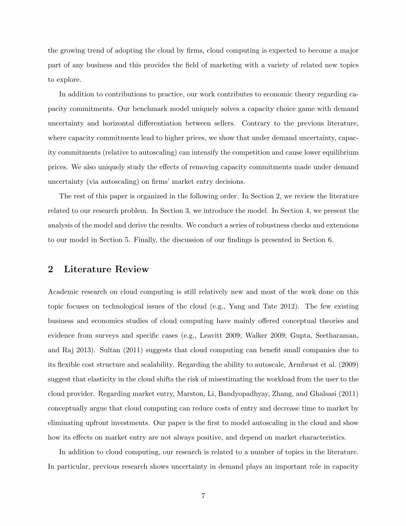
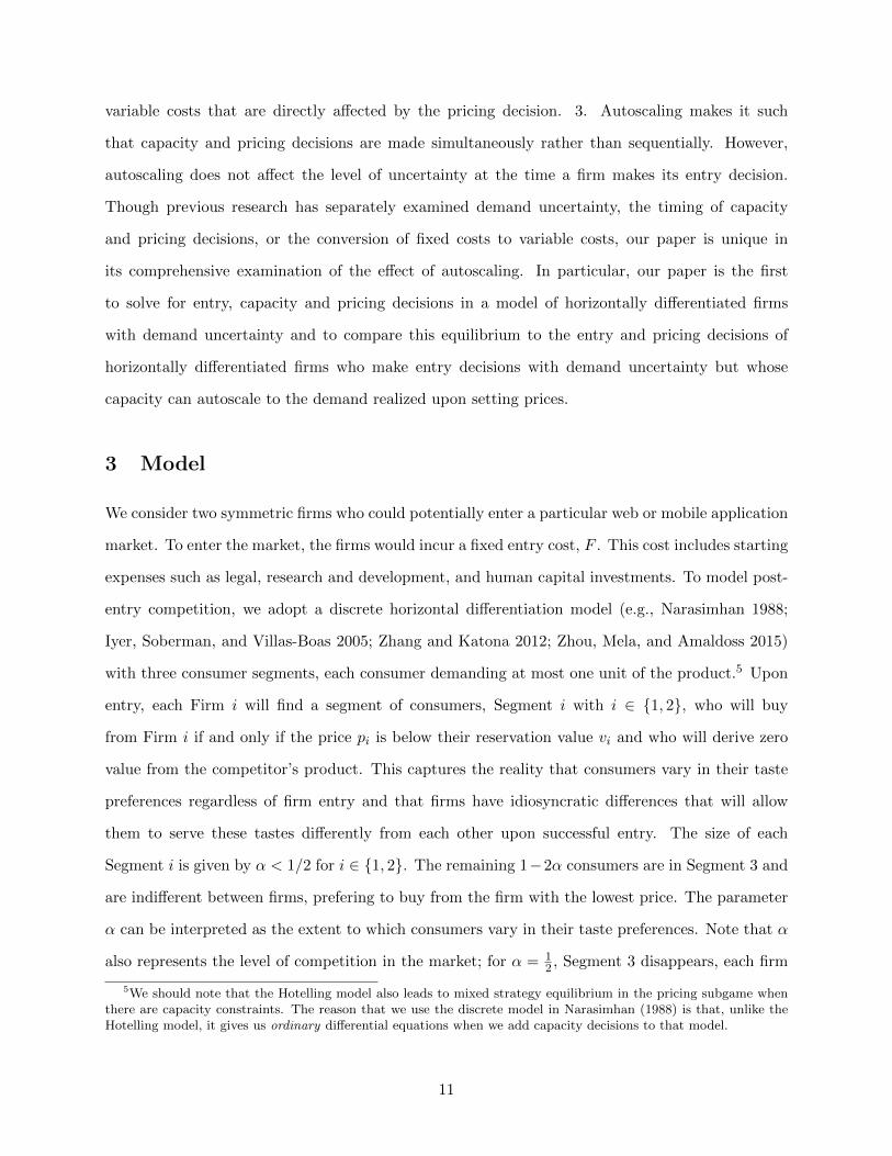
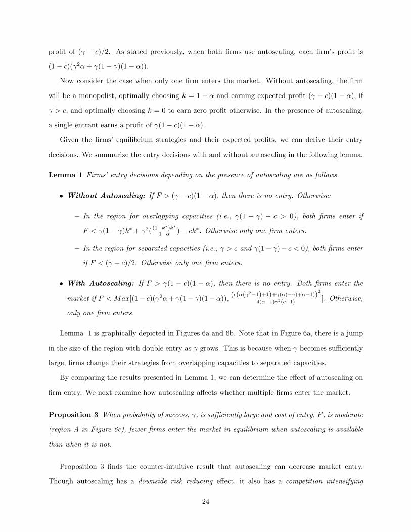
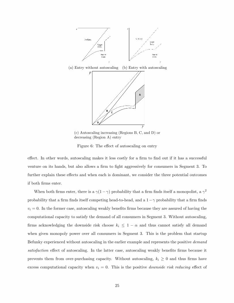
Lemma 1 is graphically depicted in Figures 6a and 6b. Note that in Figure 6a, there is a jump

in the size of the region with double entry as γ grows. This is because when γ becomes sufficiently

large, firms change their strategies from overlapping capacities to separated capacities.

By comparing the results presented in Lemma 1, we can determine the effect of autoscaling on

firm entry. We next examine how autoscaling affects whether multiple firms enter the market.

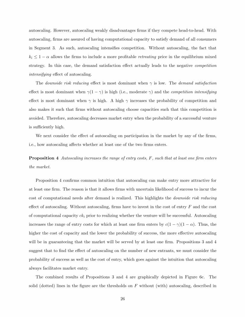
Proposition 3 When probability of success, γ, is sufficiently large and cost of entry, F , is moderate

(region A in Figure 6c), fewer firms enter the market in equilibrium when autoscaling is available

than when it is not.

Proposition 3 finds the counter-intuitive result that autoscaling can decrease market entry.

Though autoscaling has a downside risk reducing effect, it also has a competition intensifying

24

(a) Entry without autoscaling (b) Entry with autoscaling

(c) Autoscaling increasing (Regions B, C, and D) ordecreasing (Region A) entry

Figure 6: The effect of autoscaling on entry

effect. In other words, autoscaling makes it less costly for a firm to find out if it has a successful

venture on its hands, but also allows a firm to fight aggressively for consumers in Segment 3. To

further explain these effects and when each is dominant, we consider the three potential outcomes

if both firms enter.

When both firms enter, there is a γ(1−γ) probability that a firm finds itself a monopolist, a γ2

probability that a firm finds itself competing head-to-head, and a 1−γ probability that a firm finds

vi = 0. In the former case, autoscaling weakly benefits firms because they are assured of having the

computational capacity to satisfy the demand of all consumers in Segment 3. Without autoscaling,

firms acknowledging the downside risk choose ki ≤ 1 − α and thus cannot satisfy all demand

when given monopoly power over all consumers in Segment 3. This is the problem that startup

Befunky experienced without autoscaling in the earlier example and represents the positive demand

satisfaction effect of autoscaling. In the latter case, autoscaling weakly benefits firms because it

prevents them from over-purchasing capacity. Without autoscaling, ki ≥ 0 and thus firms have

excess computational capacity when vi = 0. This is the positive downside risk reducing effect of

25

autoscaling. However, autoscaling weakly disadvantages firms if they compete head-to-head. With

autoscaling, firms are assured of having computational capacity to satisfy demand of all consumers

in Segment 3. As such, autoscaling intensifies competition. Without autoscaling, the fact that

ki ≤ 1 − α allows the firms to include a more profitable retreating price in the equilibrium mixed

strategy. In this case, the demand satisfaction effect actually leads to the negative competition

intensifying effect of autoscaling.

The downside risk reducing effect is most dominant when γ is low. The demand satisfaction

effect is most dominant when γ(1 − γ) is high (i.e., moderate γ) and the competition intensifying

effect is most dominant when γ is high. A high γ increases the probability of competition and

also makes it such that firms without autoscaling choose capacities such that this competition is

avoided. Therefore, autoscaling decreases market entry when the probability of a successful venture

is sufficiently high.

We next consider the effect of autoscaling on participation in the market by any of the firms,

i.e., how autoscaling affects whether at least one of the two firms enters.

Proposition 4 Autoscaling increases the range of entry costs, F , such that at least one firm enters

the market.

Proposition 4 confirms common intuition that autoscaling can make entry more attractive for

at least one firm. The reason is that it allows firms with uncertain likelihood of success to incur the

cost of computational needs after demand is realized. This highlights the downside risk reducing

effect of autoscaling. Without autoscaling, firms have to invest in the cost of entry F and the cost

of computational capacity cki prior to realizing whether the venture will be successful. Autoscaling

increases the range of entry costs for which at least one firm enters by c(1− γ)(1− α). Thus, the

higher the cost of capacity and the lower the probability of success, the more effective autoscaling

will be in guaranteeing that the market will be served by at least one firm. Propositions 3 and 4

suggest that to find the effect of autoscaling on the number of new entrants, we must consider the

probability of success as well as the cost of entry, which goes against the intuition that autoscaling

always facilitates market entry.

The combined results of Propositions 3 and 4 are graphically depicted in Figure 6c. The

solid (dotted) lines in the figure are the thresholds on F without (with) autoscaling, described in

26

Lemma 1. As shown in this figure, there are four regions of interest. In region A, autoscaling

decreases entry due to the competition intensifying effect. Autoscaling allows one firm to be a

monopolist because the other firm cannot profitably enter given the anticipated level of competitive

intensity. In regions B and D, the market will not be served by either firm unless there is autoscaling.

In region C, a firm would have monopoly power because the downside risk of capacity pre-purchase

makes it unprofitable for a second entrant, but autoscaling alleviates this effect and results in

competing firms entering the market.15

Next, we consider the effect of autoscaling on the expected profit of the two firms entering the

market.

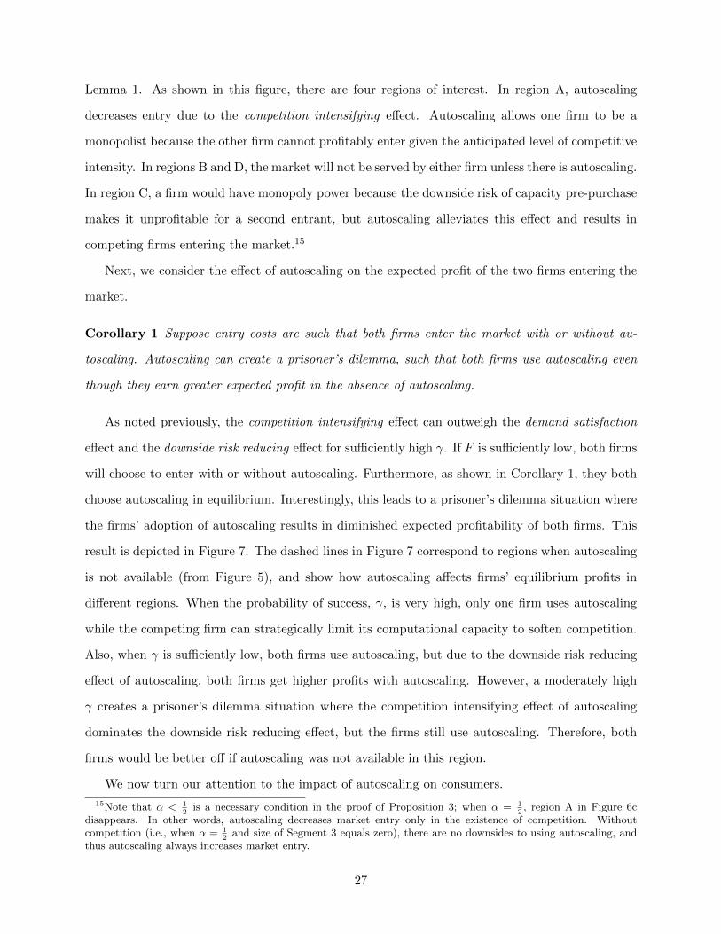
Corollary 1 Suppose entry costs are such that both firms enter the market with or without au-

toscaling. Autoscaling can create a prisoner’s dilemma, such that both firms use autoscaling even

though they earn greater expected profit in the absence of autoscaling.

As noted previously, the competition intensifying effect can outweigh the demand satisfaction

effect and the downside risk reducing effect for sufficiently high γ. If F is sufficiently low, both firms

will choose to enter with or without autoscaling. Furthermore, as shown in Corollary 1, they both

choose autoscaling in equilibrium. Interestingly, this leads to a prisoner’s dilemma situation where

the firms’ adoption of autoscaling results in diminished expected profitability of both firms. This

result is depicted in Figure 7. The dashed lines in Figure 7 correspond to regions when autoscaling

is not available (from Figure 5), and show how autoscaling affects firms’ equilibrium profits in

different regions. When the probability of success, γ, is very high, only one firm uses autoscaling

while the competing firm can strategically limit its computational capacity to soften competition.

Also, when γ is sufficiently low, both firms use autoscaling, but due to the downside risk reducing

effect of autoscaling, both firms get higher profits with autoscaling. However, a moderately high

γ creates a prisoner’s dilemma situation where the competition intensifying effect of autoscaling

dominates the downside risk reducing effect, but the firms still use autoscaling. Therefore, both

firms would be better off if autoscaling was not available in this region.

We now turn our attention to the impact of autoscaling on consumers.

15Note that α < 12

is a necessary condition in the proof of Proposition 3; when α = 12, region A in Figure 6c

disappears. In other words, autoscaling decreases market entry only in the existence of competition. Withoutcompetition (i.e., when α = 1

2and size of Segment 3 equals zero), there are no downsides to using autoscaling, and

thus autoscaling always increases market entry.

27

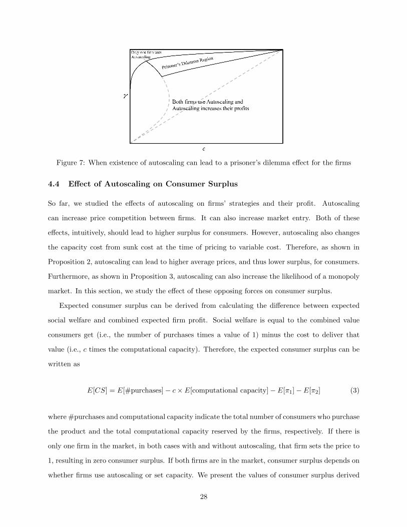
Figure 7: When existence of autoscaling can lead to a prisoner’s dilemma effect for the firms

4.4 Effect of Autoscaling on Consumer Surplus

So far, we studied the effects of autoscaling on firms’ strategies and their profit. Autoscaling

can increase price competition between firms. It can also increase market entry. Both of these

effects, intuitively, should lead to higher surplus for consumers. However, autoscaling also changes

the capacity cost from sunk cost at the time of pricing to variable cost. Therefore, as shown in

Proposition 2, autoscaling can lead to higher average prices, and thus lower surplus, for consumers.

Furthermore, as shown in Proposition 3, autoscaling can also increase the likelihood of a monopoly

market. In this section, we study the effect of these opposing forces on consumer surplus.

Expected consumer surplus can be derived from calculating the difference between expected

social welfare and combined expected firm profit. Social welfare is equal to the combined value

consumers get (i.e., the number of purchases times a value of 1) minus the cost to deliver that

value (i.e., c times the computational capacity). Therefore, the expected consumer surplus can be

written as

E[CS] = E[#purchases]− c× E[computational capacity]− E[π1]− E[π2] (3)

where #purchases and computational capacity indicate the total number of consumers who purchase

the product and the total computational capacity reserved by the firms, respectively. If there is

only one firm in the market, in both cases with and without autoscaling, that firm sets the price to

1, resulting in zero consumer surplus. If both firms are in the market, consumer surplus depends on

whether firms use autoscaling or set capacity. We present the values of consumer surplus derived

28

from Equation (3) in the Technical Appendix. Comparing across conditions, we have the following

result.

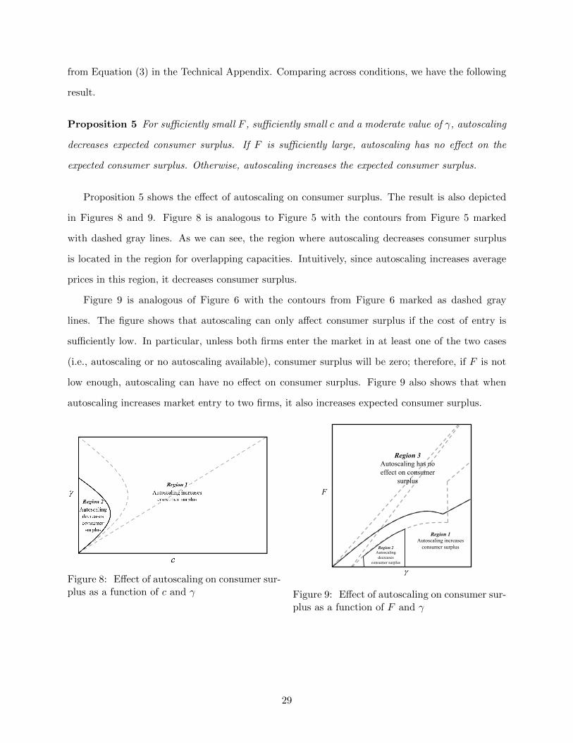
Proposition 5 For sufficiently small F , sufficiently small c and a moderate value of γ, autoscaling

decreases expected consumer surplus. If F is sufficiently large, autoscaling has no effect on the

expected consumer surplus. Otherwise, autoscaling increases the expected consumer surplus.

Proposition 5 shows the effect of autoscaling on consumer surplus. The result is also depicted

in Figures 8 and 9. Figure 8 is analogous to Figure 5 with the contours from Figure 5 marked

with dashed gray lines. As we can see, the region where autoscaling decreases consumer surplus

is located in the region for overlapping capacities. Intuitively, since autoscaling increases average

prices in this region, it decreases consumer surplus.

Figure 9 is analogous of Figure 6 with the contours from Figure 6 marked as dashed gray

lines. The figure shows that autoscaling can only affect consumer surplus if the cost of entry is

sufficiently low. In particular, unless both firms enter the market in at least one of the two cases

(i.e., autoscaling or no autoscaling available), consumer surplus will be zero; therefore, if F is not

low enough, autoscaling can have no effect on consumer surplus. Figure 9 also shows that when

autoscaling increases market entry to two firms, it also increases expected consumer surplus.

Figure 8: Effect of autoscaling on consumer sur-plus as a function of c and γ

γ

F    

Region 3 Autoscaling has no effect on consumer

surplus

Region 2 Autoscaling

decreases consumer surplus

Region 1 Autoscaling increases

consumer surplus

Figure 9: Effect of autoscaling on consumer sur-plus as a function of F and γ

29

5 Extensions

So far, we studied the effect of autoscaling on prices, profits, market entry, and consumer surplus

using a model of market entry for horizontally differentiated firms. In this section, we examine

three extensions of the model to establish the robustness of our results and obtain new insights.

First, in Section 5.1, we consider the case in which when firms do not succeed, consumers still have

positive reservation value for their offerings (Vl > 0). In the main model, we assumed an efficient

rationing rule when allocating firms’ capacity to consumer demand. In Section 5.2, we relax that

assumption by considering a proportional rationing rule. Finally, in Section 5.3, we look at the

incentives of the service provider and endogenize the price of capacity c.

5.1 Positive Low-State Value

In the main model, we assumed that consumers’ reservation value for a firm that does not succeed

is vi = 0. This assumption could seem strong as it gives monopoly power to the competitor. In

this section, we relax this assumption to show the robustness of our results. We assume that the

reservation value of consumers for each firm is Vh with probability γ and Vl with probability 1− γ,

where Vh > Vl > 0. We show that our counter-intuitive result in Proposition 3 that autoscaling

could lower entry becomes even stronger when Vl > 0.

Equilibrium Choices without Autoscaling

We use the same techniques as before to solve the pricing subgame, and to calculate the expected

profit of Firm i for given capacities. The details of how we solve the pricing subgame are provided

in the appendix. The expected profit of Firm i, where i, j ∈ {1, 2}, depends on the capacities of

30

the two firms as shown below, assuming α ≤ ki, kj ≤ 1− α.

E(πi) =

ki(−c+ γVh − γVl + Vl) if ki + kj ≤ 1

ki((ki−1)((γ−1)Vl−γVh)−ckj)kj

if ki <VlVhkj and ki + kj ≥ 1

ki(−ckj+γ2(−kj)Vh+γkjVh+γ2kjVl+γ(−kj−1)Vl+γ2Vh+Vl)kj

+ if VlVhkj < ki < kj and ki + kj ≥ 1

k2i (γ2(−Vh)+γVl−Vl)kj

+γ2k2jVl−γk2jVl−γ2kjVl+γkjVl

kj

−cki + (1− γ)γki

(Vh −

Vl(ki+kj−1)kj

)+ if Vl

Vhki < kj < ki and ki + kj ≥ 1

(1− kj)(γ2Vh + (γ − 1)2Vl

)+ (γ − 1)γ(kj − 1)Vl

(kj − 1)((γ − 1)Vl − γVh)− cki if kj <VlVhki and ki + kj ≥ 1

Given the firms’ expected profits in the pricing subgame, we can calculate the equilibrium

capacities by comparing the expected profits for each set of capacities. Assuming both firms enter

the market, equilibrium capacity choices depend on the probability of success, the low state and

high state values, and the cost of capacity as follows:

• If there is a low probability of a successful venture (i.e., γ(Vh − Vl) +Vl < c), then both firms

choose ki = 0.

• If there is a moderate probability of a successful venture (i.e., (1 − γ)γ(Vh − Vl) > c), then

the firms choose overlapping capacities such that ki + kj > 1.

• If there is a high probability of a successful venture (i.e., (1−γ)γ(Vh−Vl) < c < γ(Vh − Vl)+

Vl), then the firms choose separating capacities with the unique symmetric equilibrium being

ki = kj = 1/2.

It is interesting to note that as Vl increases, the region in which firms use separated capacities

grows. The region for separated capacities is given by (1 − γ)γ(Vh − Vl) < c < γ(Vh − Vl) + Vl.

Since we have ∂((1−γ)γ(Vh−Vl))∂Vl

< 0 and ∂(γ(Vh−Vl)+Vl)∂Vl

> 0, this region becomes larger as Vl increases.

Intuitively, this is because increasing Vl increases direct competition between a high-value firm and

a low-value firm when their capacities overlap. To avoid this competition, firms are more likely

to choose separated capacities and gain monopoly pricing power for higher Vl. Since autoscaling

breaks the firms’ ability to dampen competition through limited capacity, as we see in the next

31

section, the competition intensifying effect of autoscaling becomes stronger as Vl increases, and,

therefore, autoscaling lowers market entry in a larger region.

Equilibrium Choices with Autoscaling

When autoscaling is available, we show that one or two firms use autoscaling. The analysis when

Vl > 0 is similar to the analysis in the main model, and, hence, is relegated to the appendix. The

expected profit of Firm i when both firms use autoscaling is

E(πAA) = −αc+ (2α− 1)γ2(Vh − Vl) + (α− 1)γ(Vl − Vh) + αVl

Effect of Low-State Value on Entry

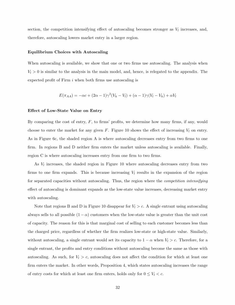
By comparing the cost of entry, F , to firms’ profits, we determine how many firms, if any, would

choose to enter the market for any given F . Figure 10 shows the effect of increasing Vl on entry.

As in Figure 6c, the shaded region A is where autoscaling decreases entry from two firms to one

firm. In regions B and D neither firm enters the market unless autoscaling is available. Finally,

region C is where autoscaling increases entry from one firm to two firms.

As Vl increases, the shaded region in Figure 10 where autoscaling decreases entry from two

firms to one firm expands. This is because increasing Vl results in the expansion of the region

for separated capacities without autoscaling. Thus, the region where the competition intensifying

effect of autoscaling is dominant expands as the low-state value increases, decreasing market entry

with autoscaling.

Note that regions B and D in Figure 10 disappear for Vl > c. A single entrant using autoscaling

always sells to all possible (1−α) customers when the low-state value is greater than the unit cost

of capacity. The reason for this is that marginal cost of selling to each customer becomes less than

the charged price, regardless of whether the firm realizes low-state or high-state value. Similarly,

without autoscaling, a single entrant would set its capacity to 1− α when Vl > c. Therefore, for a

single entrant, the profits and entry conditions without autoscaling become the same as those with

autoscaling. As such, for Vl > c, autoscaling does not affect the condition for which at least one

firm enters the market. In other words, Proposition 4, which states autoscaling increases the range

of entry costs for which at least one firm enters, holds only for 0 ≤ Vl < c.

32

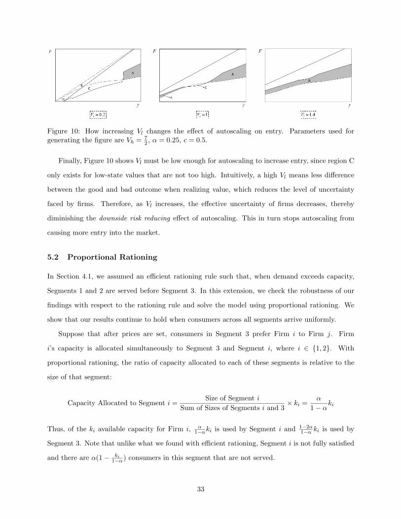
Figure 10: How increasing Vl changes the effect of autoscaling on entry. Parameters used forgenerating the figure are Vh = 7

2 , α = 0.25, c = 0.5.

Finally, Figure 10 shows Vl must be low enough for autoscaling to increase entry, since region C

only exists for low-state values that are not too high. Intuitively, a high Vl means less difference

between the good and bad outcome when realizing value, which reduces the level of uncertainty

faced by firms. Therefore, as Vl increases, the effective uncertainty of firms decreases, thereby

diminishing the downside risk reducing effect of autoscaling. This in turn stops autoscaling from

causing more entry into the market.

5.2 Proportional Rationing

In Section 4.1, we assumed an efficient rationing rule such that, when demand exceeds capacity,

Segments 1 and 2 are served before Segment 3. In this extension, we check the robustness of our

findings with respect to the rationing rule and solve the model using proportional rationing. We

show that our results continue to hold when consumers across all segments arrive uniformly.

Suppose that after prices are set, consumers in Segment 3 prefer Firm i to Firm j. Firm

i’s capacity is allocated simultaneously to Segment 3 and Segment i, where i ∈ {1, 2}. With

proportional rationing, the ratio of capacity allocated to each of these segments is relative to the

size of that segment:

Capacity Allocated to Segment i =Size of Segment i

Sum of Sizes of Segments i and 3× ki =

α

1− αki

Thus, of the ki available capacity for Firm i, α1−αki is used by Segment i and 1−2α

1−α ki is used by

Segment 3. Note that unlike what we found with efficient rationing, Segment i is not fully satisfied

and there are α(1− ki1−α) consumers in this segment that are not served.

33

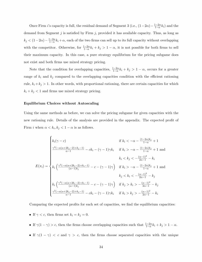
Once Firm i’s capacity is full, the residual demand of Segment 3 (i.e., (1−2α)− 1−2α1−α ki) and the

demand from Segment j is satisfied by Firm j, provided it has available capacity. Thus, as long as

kj < (1−2α)− 1−2α1−α ki+α, each of the two firms can sell up to its full capacity without overlapping

with the competitor. Otherwise, for 1−2α1−α ki + kj > 1 − α, it is not possible for both firms to sell

their maximum capacity. In this case, a pure strategy equilibrium for the pricing subgame does

not exist and both firms use mixed strategy pricing.

Note that the condition for overlapping capacities, 1−2α1−α ki + kj > 1 − α, occurs for a greater

range of ki and kj compared to the overlapping capacities condition with the efficient rationing

rule, ki+kj > 1. In other words, with proportional rationing, there are certain capacities for which

ki + kj < 1 and firms use mixed strategy pricing.

Equilibrium Choices without Autoscaling

Using the same methods as before, we can solve the pricing subgame for given capacities with the

new rationing rule. Details of the analysis are provided in the appendix. The expected profit of

Firm i when α < ki, kj < 1− α is as follows.

E(πi) =

ki(γ − c) if ki < −α− (1−2α)kj1−α + 1

γ2(−α(α+2kj−2)+kj−1)α−1 − cki − (γ − 1)γki if ki > −α− (1−2α)kj

1−α + 1 and

ki < kj < − (α−1)22α−1 − ki

ki

(γ2(−α(α+2ki−2)+ki−1)

(α−1)kj − c− (γ − 1)γ)

if ki > −α− (1−2α)kj1−α + 1 and

kj < ki < − (α−1)22α−1 − kj

ki

(γ2(−α(α+2ki−2)+ki−1)

(α−1)kj − c− (γ − 1)γ)

if kj > ki > − (α−1)22α−1 − kj

γ2(−α(α+2kj−2)+kj−1)α−1 − cki − (γ − 1)γki if ki > kj > − (α−1)2

2α−1 − ki

Comparing the expected profits for each set of capacities, we find the equilibrium capacities:

• If γ < c, then firms set ki = kj = 0.

• If γ(1− γ) > c, then the firms choose overlapping capacities such that 1−2α1−α ki + kj > 1− α.

• If γ(1 − γ) < c and γ > c, then the firms choose separated capacities with the unique

34

symmetric equilibrium being ki = kj = (α−1)22−3α .

Thus, the regions for separated and overlapping capacities have the same boundaries as in

Proposition 1, when the efficient rationing rule was used. The difference from using a proportional

rationing rule only appears in the capacities chosen within each region, not the size of each region.

Equilibrium Choices with Autoscaling

When both firms use autoscaling, the rationing rule does not affect the outcome, since neither firm

has a capacity constraint. Therefore, each firm’s profit is πaa = (1− c)(αγ2 + (1− α)(1− γ)γ

).

In the appendix, we analyze the case when one firm uses autoscaling and the other chooses

a fixed capacity. This case is affected by the rationing rule, which determines how much of the

capacity of the firm not using autoscaling is allocated to consumers in Segment 3. We find that the

profits are πan = 12(1−α)(−2γc+ c+ γ) for the firm using autoscaling and πna = (α−1)2(c−γ)2

4(1−2α)γ2(1−c) for

the firm choosing fixed capacity.

Effect of Autoscaling on Entry with Proportional Rationing

We compare the cost of entry, F , to firms’ profits, finding the number of firms that choose to enter

the market for any given F . We prove in the appendix that there exists a cutoff γ, such that

for γ > γ autoscaling decreases the range of entry costs for which both firms enter the market.

This result is similar to what we found about the effect of autoscaling on entry when the efficient

rationing rule was applied. Also, the rationing rule does not affect profits and entry conditions when

only one firm enters the market. Thus, both Propositions 3 and 4 hold with proportional rationing.

Figure 11 shows the effect of autoscaling on market entry with proportional rationing. In region

A, autoscaling decreases entry from 2 to 1 firms. In region C, autoscaling increases entry from 1

to 2 firms. In regions B and D, autoscaling increases entry from 0 to 1 and 2 firms respectively.

Comparing Figure 11 with Figure 6c, where the efficient rationing rule was used, we see that the

insights of our model for market entry remain the same with proportional rationing.

35

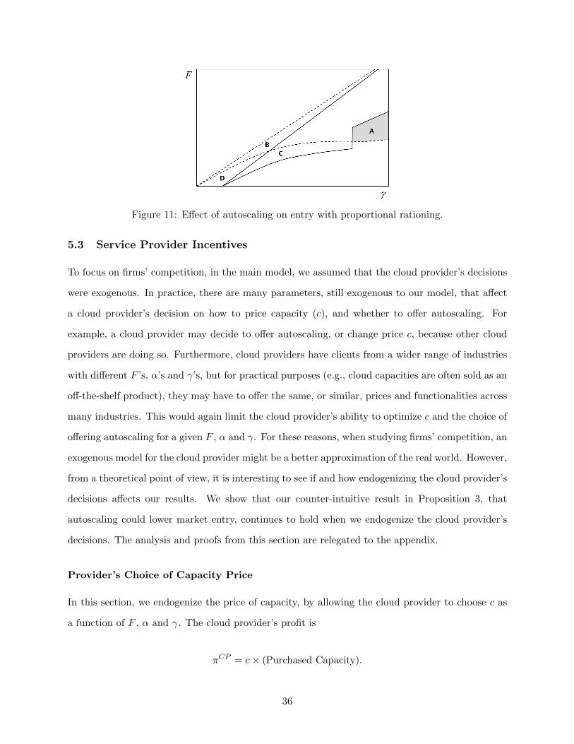
Figure 11: Effect of autoscaling on entry with proportional rationing.

5.3 Service Provider Incentives

To focus on firms’ competition, in the main model, we assumed that the cloud provider’s decisions

were exogenous. In practice, there are many parameters, still exogenous to our model, that affect

a cloud provider’s decision on how to price capacity (c), and whether to offer autoscaling. For

example, a cloud provider may decide to offer autoscaling, or change price c, because other cloud

providers are doing so. Furthermore, cloud providers have clients from a wider range of industries

with different F ’s, α’s and γ’s, but for practical purposes (e.g., cloud capacities are often sold as an

off-the-shelf product), they may have to offer the same, or similar, prices and functionalities across

many industries. This would again limit the cloud provider’s ability to optimize c and the choice of

offering autoscaling for a given F , α and γ. For these reasons, when studying firms’ competition, an

exogenous model for the cloud provider might be a better approximation of the real world. However,

from a theoretical point of view, it is interesting to see if and how endogenizing the cloud provider’s

decisions affects our results. We show that our counter-intuitive result in Proposition 3, that

autoscaling could lower market entry, continues to hold when we endogenize the cloud provider’s

decisions. The analysis and proofs from this section are relegated to the appendix.

Provider’s Choice of Capacity Price

In this section, we endogenize the price of capacity, by allowing the cloud provider to choose c as

a function of F , α and γ. The cloud provider’s profit is

πCP = c× (Purchased Capacity).

36

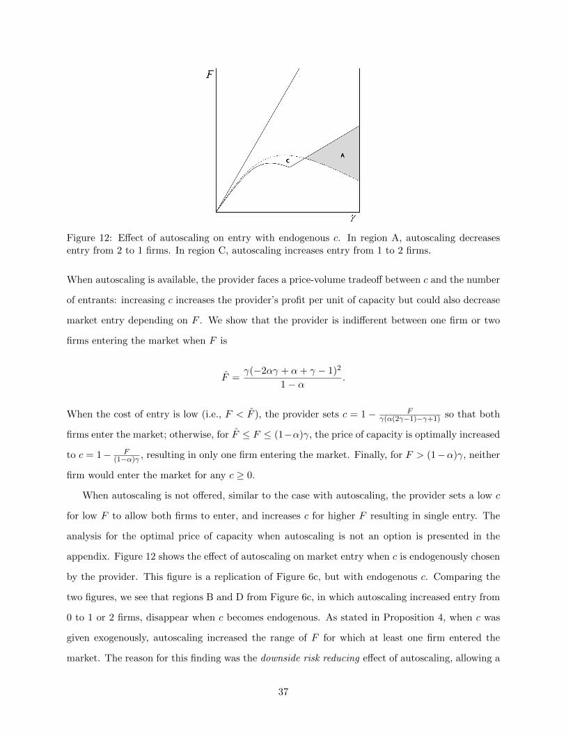
Figure 12: Effect of autoscaling on entry with endogenous c. In region A, autoscaling decreasesentry from 2 to 1 firms. In region C, autoscaling increases entry from 1 to 2 firms.

When autoscaling is available, the provider faces a price-volume tradeoff between c and the number

of entrants: increasing c increases the provider’s profit per unit of capacity but could also decrease

market entry depending on F . We show that the provider is indifferent between one firm or two

firms entering the market when F is

F =γ(−2αγ + α+ γ − 1)2

1− α.

When the cost of entry is low (i.e., F < F ), the provider sets c = 1− Fγ(α(2γ−1)−γ+1) so that both

firms enter the market; otherwise, for F ≤ F ≤ (1−α)γ, the price of capacity is optimally increased

to c = 1− F(1−α)γ , resulting in only one firm entering the market. Finally, for F > (1−α)γ, neither

firm would enter the market for any c ≥ 0.

When autoscaling is not offered, similar to the case with autoscaling, the provider sets a low c

for low F to allow both firms to enter, and increases c for higher F resulting in single entry. The

analysis for the optimal price of capacity when autoscaling is not an option is presented in the

appendix. Figure 12 shows the effect of autoscaling on market entry when c is endogenously chosen

by the provider. This figure is a replication of Figure 6c, but with endogenous c. Comparing the

two figures, we see that regions B and D from Figure 6c, in which autoscaling increased entry from

0 to 1 or 2 firms, disappear when c becomes endogenous. As stated in Proposition 4, when c was

given exogenously, autoscaling increased the range of F for which at least one firm entered the

market. The reason for this finding was the downside risk reducing effect of autoscaling, allowing a

37

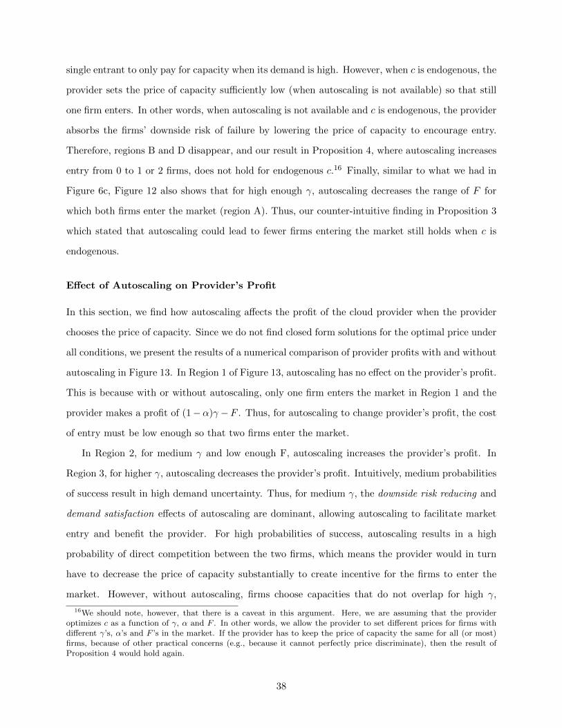
single entrant to only pay for capacity when its demand is high. However, when c is endogenous, the

provider sets the price of capacity sufficiently low (when autoscaling is not available) so that still

one firm enters. In other words, when autoscaling is not available and c is endogenous, the provider

absorbs the firms’ downside risk of failure by lowering the price of capacity to encourage entry.

Therefore, regions B and D disappear, and our result in Proposition 4, where autoscaling increases

entry from 0 to 1 or 2 firms, does not hold for endogenous c.16 Finally, similar to what we had in

Figure 6c, Figure 12 also shows that for high enough γ, autoscaling decreases the range of F for

which both firms enter the market (region A). Thus, our counter-intuitive finding in Proposition 3

which stated that autoscaling could lead to fewer firms entering the market still holds when c is

endogenous.

Effect of Autoscaling on Provider’s Profit

In this section, we find how autoscaling affects the profit of the cloud provider when the provider

chooses the price of capacity. Since we do not find closed form solutions for the optimal price under

all conditions, we present the results of a numerical comparison of provider profits with and without

autoscaling in Figure 13. In Region 1 of Figure 13, autoscaling has no effect on the provider’s profit.

This is because with or without autoscaling, only one firm enters the market in Region 1 and the

provider makes a profit of (1−α)γ −F . Thus, for autoscaling to change provider’s profit, the cost

of entry must be low enough so that two firms enter the market.

In Region 2, for medium γ and low enough F, autoscaling increases the provider’s profit. In

Region 3, for higher γ, autoscaling decreases the provider’s profit. Intuitively, medium probabilities

of success result in high demand uncertainty. Thus, for medium γ, the downside risk reducing and

demand satisfaction effects of autoscaling are dominant, allowing autoscaling to facilitate market

entry and benefit the provider. For high probabilities of success, autoscaling results in a high

probability of direct competition between the two firms, which means the provider would in turn

have to decrease the price of capacity substantially to create incentive for the firms to enter the

market. However, without autoscaling, firms choose capacities that do not overlap for high γ,

16We should note, however, that there is a caveat in this argument. Here, we are assuming that the provideroptimizes c as a function of γ, α and F . In other words, we allow the provider to set different prices for firms withdifferent γ’s, α’s and F ’s in the market. If the provider has to keep the price of capacity the same for all (or most)firms, because of other practical concerns (e.g., because it cannot perfectly price discriminate), then the result ofProposition 4 would hold again.

38

Figure 13: Effect of autoscaling on cloud provider’s profit. Region 1 denotes autoscaling does notchange providers’ profit. Region 2 denotes autoscaling increases provider’s profit. Region 3 denotesautoscaling decreases provider’s profit.

allowing the provider to choose a higher c. Thus, when γ is high, autoscaling prevents the provider

from increasing the price of capacity and earning more profit.

Figure 13 also shows the effect of changing α on the provider’s profits. As α increases, the

expected purchased capacity of a single entrant, (1 − α), decreases, making single entry a less

attractive option for the provider and shrinking Region 1.

Figure 13 confirms the intuition that for markets with considerable demand uncertainty, rep-

resented by medium γ in Region 2, autoscaling helps increase the provider’s profit and impacts

the market. Note that while autoscaling may not benefit the provider in certain industries with

little uncertainty, the provider makes the choice of offering autoscaling based on the aggregate out-

come of multiple industries with varying levels of γ and F . Also, other factors such as competition

among providers can be expected to contribute to strengthening the benefit of autoscaling for cloud

providers. Observations from the cloud computing industry indicate that autoscaling is offered by

all major cloud providers and is not an exclusive offer for only certain markets.17 A thorough

examination of such contributing factors affecting providers’ decisions is a potentially rich topic for

future research on cloud computing, but outside of the scope of this paper.

In the appendix, we show that even when the cloud provider is allowed to choose two separate

capacity prices, ck for fixed pre-purchased capacity and ca for autoscaling capacity, the insights are

similar to those from Figure 13.

17www.knowthecloud.com/Providers/auto-scaling-providers.html, accessed February 2017.

39

6 Discussion

The emergence of cloud computing and its feature of autoscaling has the potential to influence the

entry of web-based firms into new markets. Before autoscaling was available, firms needed to invest

heavily in computational capacity before entering a new market so that they could serve highly

unpredictable demand levels. The uncertainty in demand meant that the capacity chosen by firms

could be more or less than the actual needs, resulting in extra costs or unfulfilled demand. However,

autoscaling allows the new entrants a flexible capacity such that the cloud provider will designate

the specific computational resources as the actual demand and required resources are realized. This

feature can help new entrants to the market pay only for the capacity that is required to meet their

demand, reducing the disadvantages of uncertainty in demand. In this paper, we find the effects of

autoscaling on entry decisions of web-based firms, their prices, their capacity decisions, and their

profits.

Our model shows how the demand satisfaction effect of autoscaling, in which firms can be

assured of having capacity to satisfy demand, turns out to be a double-edged sword in that it

frees competing firms to aggressively pursue customers. Our research identifies this competition

intensifying effect of autoscaling and establishes the conditions under which this effect will outweigh

the positive effects of autoscaling. This has several important implications for web-based firms and

their product launch strategies.

The results can help guide pricing decisions by firms launching a new product with autoscaling.

We find that autoscaling will increase the average launch prices if the probability of a successful

venture is not too high. In this case, autoscaling decreases a firm’s costs, but these savings are

not passed on to consumers because autoscaling converts a sunk fixed cost into a variable cost

that a firm incurs if and only if it attracts more customers. As a consequence, price competition

is dampened by autoscaling in the case that entrants would otherwise choose excessive capacities.

However, if the probability of a successful venture is sufficiently high, firms would optimally limit

their capacities to dampen competition in the absence of autoscaling. In this case, autoscaling gives

the competing firms freedom to aggressively pursue customers with price and thus can decrease

average prices.

The trade-off between the intensified competition and the reduced downside risk of failure affects

40

firms’ decisions on whether to enter the market. In particular, when the probability of success is

sufficiently high, the increased competition effect of autoscaling dominates the decreased downside

risk of failure. As a result, while autoscaling facilitates the entry for one firm, it deters a second

firm from simultaneously entering the market. Our findings expand the market entry literature by

looking at the topic from the new angle of capacity choice before versus after demand is realized.

Our research also guides managers of web-based firms with their response to the introduction

of autoscaling and cloud computing. The research shows if the probability of success is moderately

high, autoscaling leads to a prisoner’s dilemma situation where both entrants adopt autoscaling,

but they would have been better off if both had avoided it. Our findings suggest that in industries

where cost of entry is relatively low, the introduction of the autoscaling feature in cloud computing

can reduce the profit of new entrants to the market even though it decreases their downside risk of

failure.

Autoscaling could also have positive or negative effects on consumer surplus. On the one hand,

it can increase price competition between the firms and facilitate their entry, both of which lead to

higher consumer surplus. On the other hand, autoscaling can lower consumer surplus by dampening

price competition or by reducing the number of firms that enter the market. Our results show that

when cost of entry is low and probability of success is moderate, autoscaling decreases expected

consumer surplus.

Overall, our results highlight how web-based firms should use information on cost of entry,

probability of success, cost of capacity and level of differentiation to evaluate their entry decisions,

capacity commitments and pricing strategies in the presence of autoscaling. Our research is one

of the first to consider the marketing aspects of cloud computing and autoscaling. With the rapid

adoption of cloud computing by firms across different industries, marketing and economics research

on the cloud can be a rich and important topic of study for future research.

References

[1] Armbrust, M., A. Fox, R. Griffith, A. Joseph, R. Katz, A. Konwinski, G. Lee, D. Patterson, A.Rabkin, and I. Stoica. 2009. “Above the clouds: A Berkeley View of Cloud Computing.” Dept.Electrical Eng. and Comput. Sciences, University of California, Berkeley, Rep. UCB/EECS28, 13.

41

[2] Anand, K. S. and K. Girotra. 2007. “The Strategic Perils of Delayed Differentiation.” Man-agement Science 53(5): 697-712.

[3] Anupindi, R. and L. Jiang. 2008. “Capacity Investment Under Postponement Strategies, Mar-ket Competition, and Demand Uncertainty.” Management Science 54(11): 1876-1890.

[4] Biyalogorsky, E., and O. Koenigsberg. 2014. “The Design and Introduction of Product LinesWhen Consumer Valuations are Uncertain.” Production and Operations Management 23(9):1539-1548.

[5] Bort, C. 2015. “Google Has Nabbed Some Huge Customers for its Most Important NewBusiness Cloud Computing.” http://www.businessinsider.com/google-names-huge-companies-using-its-cloud-2015-6, accessed September 2016.

[6] Buehler, S. and J. Haucap. 2006. “Strategic Outsourcing Revisited.” Journal of EconomicBehavior and Organization 61(3) 325-338.

[7] Burke, A. and S. Hussels. 2013. “How Competition Strengthens Start-ups.” Harvard BusinessReview 91(3), 24-25.

[8] Che, H., C. Narasimhan, and V. Padmanabhan. 2010. “Leveraging Uncertainty Through Back-order.” Quantitative Marketing and Economics 8(3): 365-392.

[9] Chen, P. and S. Wu. 2013. “the Impact and Implications of On-Demand Services on MarketStructure.” Information Systems Research 24(3): 750-767.

[10] Chen, Y. and G. Iyer. 2002. “Consumer Addressability and Customized Pricing.” MarketingScience 21(2): 197-208.

[11] Columbus, L. 2015. “Roundup of Cloud Computing Forecasts and Market Estimates Q3 Up-date, 2015.” www.forbes.com/sites/louiscolumbus/2015/09/27/roundup-of-cloud-computing-forecasts-and-market-estimates-q3-update-2015/, accessed September 2016.

[12] Desai, P., O. Koenigsberg, and D. Purohit. 2007. “The Role of Production Lead Time andDemand Uncertainty in Marketing Durable Goods.” Management Science 53(1): 150-158.

[13] Desai, P., O. Koenigsberg, and D. Purohit. 2010. “Forward Buying by Retailers.” Journal ofMarketing Research 47(1): 90-102.

[14] Ferguson, M. and O. Koenigsberg. 2007. “How Should a Firm Manage Deteriorating Inven-tory.” Production and Operations Management 16(3): 306-321.

[15] Flood, G. 2013. “Gartner Tells Outsourcers: Embrace Cloud Or Die.”http://www.informationweek.com/cloud/infrastructure-as-a-service/gartner-tells-outsourcers-embrace-cloud-or-die/d/d-id/1110991, accessed September 2016.

[16] Gaudin, S. 2015. “AWS Assures Customers it’s Atop the Cloud.”http://www.computerworld.com/article/2990119/cloud-computing/aws-assures-customers-theyre-atop-the-cloud.html, accessed September 2016.

[17] Goyal, M. and S. Netessine. 2007. “Strategic Technology Choice and Capacity Investmentunder Demand Uncertainty.” Management Science 53(2): 192-207.

[18] Griffith, E. 2014. “Why Startups Fail, According to Their Founders.” Forbes Sep, 25.

42

[19] Gupta, P., A. Seetharaman, and J. R. Raj. 2013. “The Usage and Adoption of Cloud Com-puting by Small and Medium Businesses.” International Journal of Information Management33(5): 861-874.

[20] Hassani, S. 2009. Mathematical Methods for Students of Physics and Related Fields (2nd ed.).New York, NY: Springer. Chapter 5.

[21] Iyer, G., D. Soberman, and J. Villas-Boas. 2005. “The Targeting of Advertising.” MarketingScience 24(3): 461-476.

[22] Joshi, Y., D. Reibstein, and J. Zhang. 2009. “Optimal Entry Timing in Markets with SocialInfluence.” Management Science 55(6): 926-939.

[23] Klems, M., J. Nimis, and S. Tai. 2008. “Do Clouds Compute? A Framework for Estimatingthe Value of Cloud Computing.” Workshop on E-Business: Designing E-Business Systems.Markets, Services, and Networks 22: 110-123.

[24] Kreps, D. and J. Scheinkman. 1983. “Quantity Precommitments and Bertrand CompetitionYield Cournot Outcomes.” The Bell Journal of Economics 14(2): 326-337.

[25] Leavitt, N. 2009. “Is Cloud Computing Really Ready For Prime Time?” Computer (1): 15-20.

[26] Lilien, G. and E. Yoon. 1990. “The Timing of Competitive Market Entry: An ExploratoryStudy of New Industrial Products.” Management Science 36(5): 568-585.

[27] Marston, S., Z. Li, S. Bandyopadhyay, J. Zhang, and A. Ghalsasi. 2011. “Cloud Computing:The Business Perspective.” Decision Support Systems 51(1): 176-189.

[28] Milgrom, P. and J. Roberts. 1982. “Limit Pricing and Entry under Incomplete Information:An Equilibrium Analysis.” Econometrica 50(2): 443-459.

[29] Narasimhan, C. and J. Zhang. 2000. “Market Entry Strategy Under Firm Heterogeneity andAsymmetric Payoffs.” Marketing Science 19(4): 313-327.

[30] Narasimhan, C. 1988. “Competitive Promotional Strategies.” Journal of Business 61(4): 427-449.

[31] Nasser, S. and D. Turcic. 2015. “To Commit or Not to Commit: Revisiting Quantity vs. PriceCompetition in a Differentiated Industry.” Management Science 62(6): 1719-1733..

[32] Nickelsburg, M. 2016. “Startup Spotlight: BeFunky makes online photo editing and graphicdesign simple.” http://www.geekwire.com/2016/befunky/, accessed September 2016.

[33] Ofek, E. and O. Turut. 2013. “Vaporware, Suddenware, and Trueware: New Product Prean-nouncements Under Market Uncertainty.” Marketing Science 32(2): 342-355.

[34] Poepsel, M. 2008. “Customers Are Won or Lost in One Second, Finds New AberdeenReport” http://www.prnewswire.com/news-releases/customers-are-won-or-lost-in-one-second-finds-new-aberdeen-report-65399152.html, accessed September 2016.

[35] Ray, T. 2013. “Salesforce, Google, Amazon Cloud Winners, Says Piper; Microsoft Straddlesthe Line.” blogs.barrons.com Oct, 17.

43

[36] Reynolds, S. and B. Wilson. 2000. “Bertrand-Edgeworth Competition, Demand Uncertainty,and Asymmetric Outcomes.” Journal of Economic Theory 92: 122-141.

[37] Shy, O. and R. Stenbacka. 2003. “Strategic outsourcing.” Journal of Economic Behavior andOrganization 50(2):203-224.

[38] Spence, M. 1977. “Entry, Capacity, Investment and Oligopolistic Pricing.” The Bell Journalof Economics 8(2): 534-544.

[39] Sultan, N. A. 2011. “Reaching for the Cloud: How SMEs Can Manage.” International journalof information management 31(3):272-278.

[40] Swinney, R., G. Cachon., and S. Netessine. 2011. “Capacity Investment Timing by Start-upsand Established Firms in New Markets.” Management Science 57(4): 763-777.

[41] Tirole, J. 1988. The Theory of Industrial Organization. Cambridge, MA: MIT Press.

[42] Van Mieghem, J. and M. Dada. 1999. “Price Versus Production Postponement: Capacity andCompetition.” Management Science 45(12):1631-1649.

[43] Walker, E. 2009. “The Real Cost of a CPU Hour.” Computer (4): 35-41.

[44] Weaver, L. 2015. “Why GE is moving nearly 9,000 apps to the public cloud.”https://enterprisersproject.com/article/2015/10/why-ge-s-moving-nearly-9000-apps-public-cloud, accessed September 2016.

[45] Work, S. 2011. “How Loading Time Affects Your Bottom Line.”https://blog.kissmetrics.com/loading-time/, accessed September 2016.

[46] Yang, H., and M. Tate. 2012. “A Descriptive Literature Review and Classification of CloudComputing Research.” Communications of the Association for Information Systems 31(2):35-60.

[47] Zhang, K. and Z. Katona. 2012. “Contextual Advertising.” Marketing Science 31(6): 980-994.

[48] Zhou, B., C. Mela, and W. Amaldoss. 2015. “Do Firms Endowed with Greater StrategicCapability Earn Higher Profits?” Journal of Marketing Research 52(3): 325-336.

A Technical Appendix

A.1 Proof of Proposition 1

If γ < c, then expected profit is strictly decreasing in capacity for any capacity chosen by the

competition. Therefore, each firm optimally chooses zero capacity.

If γ > c, then for any k2 < 1 − α, expected profit is increasing in k1 for any k1 < 1 − k2.

Therefore, we can rule out any k1 + k2 < 1. First consider γ(1 − γ) < c. Suppose there were

a symmetric equilibrium in which k1 + k2 > 1. By definition, this implies that k1 > 1/2 which

44

means Firm 1 earns greater expected profit by deviating downward. Therefore, the only potential

symmetric equilibrium requires k1 + k2 = 1. If Firm 1 deviates upward, its expected change in

profit is γ(1− γ)− c < 0.

If γ(1− γ) > c, then k1 + k2 = 1 is no longer an equilibrium because either firm can profitably

deviate to harvest the potential of monopoly power. We can therefore focus our attention on

k1 + k2 > 1. If k2 > k1, then Firm 2’s expected profit is strictly increasing in k2 until k2 =

1 − α and is strictly decreasing for any k2 > 1 − α. If k2 > k1, Firm 1’s expected profit for

any k1 < 1 − α is given by γ(1 − γ) + γ2 (1−k1)k1k2− k1c, which is concave in k1 and maximized

at k1 = γ(1−α(1−γ))−c(1−α)2γ2

. Note this value of k1 is in fact less than 1 − α if and only if c >

γ(1+α(γ−1))1−α − 2γ2. We verify that Firm 2 cannot benefit from a global deviation undercutting k1 at

this level. Supposing that Firm 2 deviates to a lower capacity than Firm 1, its profit would become

k2

(−c+ γ

(1− γ − 2γ3(−1+k2)

c(−1+α)+γ(1+(−1+γ)α)

)), which is maximized at

k2 = −c2(−1 + α) + cγ(2 + 2α(−1 + γ)− γ) + γ2

(−1 + α+ γ − 2αγ + (−2 + α)γ2

)4γ4

.

It is easily shown that any values of c that allow for k2 < k1 will result in Firm 2’s profit at k2

(i.e.,(c2(−1+α)+cγ(2−γ+2(−1+γ)α)+γ2(−1+γ+γ2(−2+α)+α−2γα))

2

8γ4(c(−1+α)+γ(1+(−1+γ)α)) ) to be less than Firm 2’s profit at our

equilibrium.

If c < γ(1+α(γ−1))1−α − 2γ2, then neither firm benefits from deviating from kj = 1 − α. Thus, k∗

from Proposition 1 is defined as k∗ = Min[γ(1−α(1−γ))−c(1−α)2γ2

, 1− α].

A.2 Proof for Firms’ Decision to Use Autoscaling

In this section, we consider the firms’ choice of using autoscaling when autoscaling is available to

see how many firms, if any, use autoscaling.

We begin with the case when only one firm uses autoscaling. Without loss of generality, we

assume that Firm 2 adopts autoscaling and Firm 1 chooses capacity k1. We start by showing that

this game does not have a pure strategy pricing equilibrium. Assume for sake of contradiction that

the firms use prices p1 and p2 in a pure strategy equilibrium. If p1 6= p2, then the firm with a lower

price can benefit from deviating by increasing its price to p1+p22 . If p1 = p2, then Firm 2 can benefit

from deviating by decreasing its price to p2− ε, for sufficiently small ε, to acquire all consumers in

45

Segment 3. Therefore, a pure strategy equilibrium cannot exist.

Next, we find a mixed strategy equilibrium for this game. Provided k1 ≤ 1 − α, Firm 2 can

choose to attack with a price that clears its capacity or retreat with a price 1 that harvests the

value from the 1− k1 consumers that Firm 1 cannot serve due to its capacity constraint. Let z′′ be

the price at which Firm 2 is indifferent between attacking to sell to 1−α consumers at price z′′ and

retreating to sell to 1− k1 consumers at price 1. We have (1− k1)(1− c) = (1− α)(z′′ − c) which

gives us z′′ = αc−ck1+(k1−1)α−1 . In equilibrium, both firms use a mixed strategy with prices ranging

from z′′ to 1. Suppose that Hi(.) is the cumulative distribution function of prices used by Firm i.

The profit of Firm 1 earned by setting price x is

π1(x) = H2(x)αx+ (1−H2(x))k1x− k1c

Using equilibrium conditions, we know that the derivative of this function with respect to x must

be zero for x ∈ (z′′, 1). By solving the differential equation we get

H2(x) =

0 if x < z′′

k1(−ck1+(−1+k1)+α(c−x)+x)(−1+α)(α−k1)x if z′′ ≤ x < 1

1 if x ≥ 1

Similarly, the profit of Firm 2 earned by setting price x is

π2(x) = H1(x)(1− k1)(x− c) + (1−H1(x))(1− α)(x− c)

By setting the derivative with respect to x to zero for x ∈ (z′′, 1) and solving the differential

equation, we get

H1(x) =

0 if x < z′′

−ck1+(−1+k1)+α(c−x)+x(k1−α)(x−c) if z′′ ≤ x < 1

1 if x ≥ 1

Prior to the pricing game, the optimal capacity k1 that maximizes expected profit for Firm 1

46

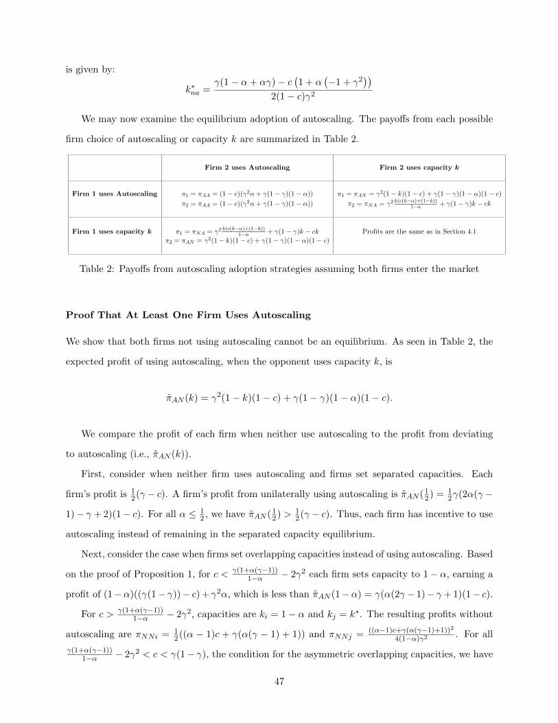
is given by:

k∗na =γ(1− α+ αγ)− c

(1 + α

(−1 + γ2

))2(1− c)γ2

We may now examine the equilibrium adoption of autoscaling. The payoffs from each possible

firm choice of autoscaling or capacity k are summarized in Table 2.

Firm 2 uses Autoscaling Firm 2 uses capacity k

Firm 1 uses Autoscaling π1 = πAA = (1− c)(γ2α+ γ(1− γ)(1− α)) π1 = πAN = γ2(1− k)(1− c) + γ(1− γ)(1− α)(1− c)π2 = πAA = (1− c)(γ2α+ γ(1− γ)(1− α)) π2 = πNA = γ2 k(c(k−α)+(1−k))

1−α + γ(1− γ)k − ck

Firm 1 uses capacity k π1 = πNA = γ2 k(c(k−α)+(1−k))1−α + γ(1− γ)k − ck Profits are the same as in Section 4.1

π2 = πAN = γ2(1− k)(1− c) + γ(1− γ)(1− α)(1− c)

Table 2: Payoffs from autoscaling adoption strategies assuming both firms enter the market

Proof That At Least One Firm Uses Autoscaling

We show that both firms not using autoscaling cannot be an equilibrium. As seen in Table 2, the

expected profit of using autoscaling, when the opponent uses capacity k, is

πAN (k) = γ2(1− k)(1− c) + γ(1− γ)(1− α)(1− c).

We compare the profit of each firm when neither use autoscaling to the profit from deviating

to autoscaling (i.e., πAN (k)).

First, consider when neither firm uses autoscaling and firms set separated capacities. Each

firm’s profit is 12(γ − c). A firm’s profit from unilaterally using autoscaling is πAN (12) = 1

2γ(2α(γ −

1)− γ + 2)(1− c). For all α ≤ 12 , we have πAN (12) > 1

2(γ − c). Thus, each firm has incentive to use

autoscaling instead of remaining in the separated capacity equilibrium.

Next, consider the case when firms set overlapping capacities instead of using autoscaling. Based

on the proof of Proposition 1, for c < γ(1+α(γ−1))1−α − 2γ2 each firm sets capacity to 1− α, earning a

profit of (1−α)((γ(1− γ))− c) + γ2α, which is less than πAN (1−α) = γ(α(2γ− 1)− γ+ 1)(1− c).

For c > γ(1+α(γ−1))1−α − 2γ2, capacities are ki = 1− α and kj = k∗. The resulting profits without

autoscaling are πNNi = 12((α − 1)c + γ(α(γ − 1) + 1)) and πNNj = ((α−1)c+γ(α(γ−1)+1))2

4(1−α)γ2 . For all

γ(1+α(γ−1))1−α − 2γ2 < c < γ(1− γ), the condition for the asymmetric overlapping capacities, we have

47

πNNi < πAN (k∗) and πNNj < πAN (1−α). Therefore, deviating to autoscaling is strictly profitable

for each firm and both firms using fixed capacities cannot be an equilibrium.

Intuitively, when both firms set capacity constraints, competition is restricted and firms set

high prices. Thus, it is always beneficial to react to a fixed capacity by using autoscaling and

undercutting the price of the opposition to win over Segment 3.

Proof for the Choice of Using Autoscaling

Given the fact that at least one firm uses autoscaling in equilibrium, we examine whether both firms

use autoscaling or only one, by comparing the profits from Table 2. If Firm 2 adopts autoscaling,

Firm 1’s best response is to adopt autoscaling if and only if

(1− c)(γ2α+ γ(1− γ)(1− α)) ≥(c(α(γ2 − 1

)+ 1)

+ γ(α(−γ) + α− 1))2

4(1− α)γ2(1− c),

where the right hand side of the inequality is Firm 1’s profit if it chooses the best possible capacity

k, given by k∗na =c(α(γ2−1)+1)+γ(α−1−αγ)

2γ2(c−1) , to Firm 2’s autoscaling decision.

Thus, only one firm uses autoscaling when γ > (1− α)/(2− 3α) and c < c, where c is defined

as follows:

c∆=

γ2(−3αγ + α+ 2γ − 1)2

2(1− γ)√

(1− α)3γ3(2αγ − α− γ + 1) + γ ((2− 3α)2γ3 + ((9− 5α)α− 4)γ2 − (α− 1)αγ + (α− 1)2)

For c > c or γ < (1− α)/(2− 3α), both firms will choose autoscaling.

A.3 Proof of Proposition 2

We start by comparing average prices with and without autoscaling in the region for overlapping capacities.

Based on the proof of Proposition 1, when c < γ(1+α(γ−1))1−α −2γ2, both firms set their capacities equal to 1−α

without autoscaling. The cumulative distribution function of prices set by each firm is F (x) = (1−α)x+α(1−2α)x .

Thus, the probability density function equals f(x) = αx2(1−2α) and the average price of each firm is pNN =∫ 1

zf(x)x dx =

α log( 1−αα )

1−2α . Now suppose autoscaling is offered in this region. For c < γ(1+α(γ−1))1−α − 2γ2, we

have γ < (1 − α)/(2 − 3α). As shown in the proof of the choice of using autoscaling, when autoscaling

is offered and γ < (1 − α)/(2 − 3α), both firms use autoscaling. With both firms using autoscaling, the

probability density function of the price of each firm equals g(x) = α(1−c)(1−2α)(x−c)2 and the average price of each

firm becomes pAA =∫ 1

z′g(x)x dx =

(1−2α)c+α log( 1−αα )(1−c)

1−2α . Thus we have pAA − pNN = c(1 − α log( 1−αα )

1−2α ).

48

We know that log(s) < s − 1, for any s > 1, . Allowing s = 1−αα , we show that log( 1−α

α ) < 1−2αα , thus

pAA > pNN .

Next consider the region for separated capacities. Without autoscaling, k1 + k2 = 1 and both firms

set their price equal to 1. When both firms use autoscaling, the average price equals pAA. As we showed,

log( 1−αα ) < 1−2α

α . Thus, pAA =(1−2α)c+α log( 1−α

α )(1−c)1−2α < 1.

When only one firm (Firm 2) uses autoscaling and the other (Firm 1) chooses capacity k1, the prob-

ability density function of Firm 1’s price equals h1(x) = − (k1−1)(c−1)(α−k1)(c−x)2 and its average price is pNA =∫ 1

z′′h1(x)x dx = c +

(1−k1)(1−c) log(

1−α1−k1

)k1−α . For all s > 0, we know that s log(s) > s − 1. Allowing s = 1−α

1−k1 ,

we have α−k1k1−1 <

(1−α)Log((1−α)/(1−k1))(1−k1) and pNA < 1.

For Firm 2, the probability density function is h2(x) = k1(−αc+ck1−k1+1)(α−1)x2(α−k1) +

(1− k1(c−1)

(α−1)

)δ(x − 1) and

the average price equals pAN =∫ 1

z′′h2(x)x dx =

(α−k1)((α+k1−1)−ck1)+k1(−αc+ck1−k1+1) log(

(1−α)−αc+ck1−k1+1

)(α−1)(α−k1) . We

know that log(s) < s − 1, for any s > 1. Allowing s = (1−α)c(k1−α)+(1−k1) , we find log

((1−α)

−αc+ck1−k1+1

)<

(1−α)−αc+ck1−k1+1 − 1 and therefore, pAN < 1. Thus, autoscaling decreases average prices in the region for

separated capacities.

A.4 Proof of Proposition 3

We compare the cut-offs on F such that both firms enter. Let FAA denote the cut-off for two firms to enter

with autoscaling, FNA denote the cut-off for two firms to enter when only one firm uses autoscaling, and

FNN denote the cut-off for two firms to enter when autoscaling is not available.

Comparing the profits from Table 2 in the presence of autoscaling, it is straightforward to show πNA <

πAN . Thus, if the subgame equilibrium involves only one firm choosing autoscaling, both firms will enter

if F < πNA. Both firms will choose autoscaling if πNA < πAA. As such, both firms will enter if F <

Max[πNA, πAA].

First consider the two cases in which γ(1 − γ) > c. If c < γ(1+α(γ−1))1−α − 2γ2, then 0 < c < 1 requires

γ < (1−α)/(2−3α). Therefore, both firms will use autoscaling if autoscaling is available. Thus, FAA−FNN =

c(1 − α + γ(1 − γ − α + 2αγ)), which is decreasing in α and positive at α = 1/2 and therefore positive for

all α < 1/2. If c > γ(1+α(γ−1))1−α − 2γ2, FAA − FNN is positive for c > c, where both firms use autoscaling.

Also, FNA > FNN for γ(1− γ) > c. Thus, in the region for overlapping capacities, the cutoff F for two firms

entering is bigger with autoscaling.

Now consider when γ > c and γ(1−γ) < c. In this case, FAA−FNN = γ(1−c)(1−α−γ(1−2α)−(γ−c)/2

which is convex in γ, equal to −(1 − c)(1 − 2α)/2 < 0 when evaluated at γ = 1, decreasing in γ through

γ = 1, and equal to zero at γAA =(1−2α)−2c(1−α)+

√8c(1−c)(1−2α)+(1−2c(1−α)−2α)2

4(1−c)(1−2α) . Therefore, FAA − FNN

is negative for any γ > γAA.

49

Also for γ > c and γ(1− γ) < c, we have FNA−FNN =(c(α(γ2−1)+1)+γ(α(−γ)+α−1))

2

4(α−1)γ2(c−1) − 12 (γ− c), which

is equal to ((−1 + 2α)(c − 1))/(4(−1 + α)) < 0 at γ = 1. Also, ∂(FNA−FNN )∂γ equals (2α−1)(c−1)

2(α−1) < 0 at

γ = 1. We find FNA = FNN has one root between γ = 0 and γ = 1, which is γNA = (1−α)(1−α+√

1−2α)2α2(c−1) +√

(α−1)(α3(1−2c)2+α2(4(√

1−2α−1)c2−4(√

1−2α−1)c+(2√

1−2α−5))+2(3−2√

1−2α)α+2(√

1−2α−1))2α2(1−c) . Therefore, FNA −

FNN is negative for any γ > γNA.

Thus, autoscaling decreases the range of F such that both firms enter for γ > γ = Max[γAA, γNA].

A.5 Proof of Proposition 4

Suppose autoscaling is not available. A firm will enter if its expected profit is greater than its entry cost.

A firm’s best response to its competitor not entering the market is to enter the market, if and only if

F < (γ − c)(1 − α). Supposing one firm enters the market, the remaining firm’s best response to its

competitor’s entry is to also enter the market provided the expected profit earned when competing is greater

than the cost of entry. The anticipated payoffs associated with being one of two firms entering are reported

in Section 4.3 and the conditions on F are presented in Lemma 1.

If only one firm enters, this firm will enjoy monopoly power over (1− α) consumers with probability γ.

Using autoscaling, the firm’s profit equals to γ(1 − c)(1 − α), which is strictly larger than (γ − c)(1 − α),

the profit earned without autoscaling, for any γ > 0. With autoscaling, at least one firm enters the market

if and only if F < FA ≡ γ(1 − c)(1 − α) whereas without autoscaling at least one firm enters if and only if

F < FN ≡ (γ − c)(1− α).

A.6 Proof of Corollary 1

We show that for sufficiently small F (such that both firms enter the market), when γ > c, γ(1−γ) < c, and

πNA < πAA < γ−c2 , we have a prisoner’s dilemma situation where both firms use autoscaling, even though

their profits would be higher if autoscaling was not available.

When γ > c and γ(1 − γ) < c, firms set separated capacities, and each earn expected profit γ−c2 , if

autoscaling is not available. However, when autoscaling is available, since πNA < πAA, both firms use

autoscaling and each earn πAA < γ−c2 in equilibrium, which creates the prisoner’s dilemma. Now, we have

to prove that all these conditions can be satisfied at the same time to show that the described region, in

which prisoner’s dilemma happens, actually exists.

Let γ = 1−α2−3α . After algebraic simplifications, we have both firms using autoscaling in equilibrium (i.e.,

πNA < πAA) if and only if c < 4(α−1)2

10α2−15α+6 . Furthermore, using algebraic simplifications, the expected

profit of autoscaling equilibrium for each firm is lower than that when firms do not use autoscaling (i.e.,

πAA < γ−c2 ) if and only if c > (α−1)α

α2+2α−2 . It is easy to see that (α−1)αα2+2α−2 < 4(α−1)2

10α2−15α+6 for any α ≤ 1/2.

50

Therefore, when c ∈ ( (α−1)αα2+2α−2 ,

4(α−1)2

10α2−15α+6 ), the prisoner’s dilemma situation holds.

A.7 Proof of Proposition 5

If c > c, then both firms would choose autoscaling upon entry and consumer surplus is E[CSAA] = γ2(1 −

c)(1− 2α), if F < (1− c)((1− α)(1− γ)γ + αγ2).

If c < c, then only one firm would choose autoscaling upon entry and the other chooses kna =

c(α(γ2−1)+1)+γ(α(−γ)+α−1)

2γ2(c−1) . The expected capacity of the firm using autoscaling is

E[kan] = −(kna − 1)kna(c− 1)

(c(c− 1)(kna − α) + (c(α− kna) + (kna − 1)) log

((kna−1)

c(α−kna)+(kna−1)

))(α− 1)c2(kna − α)

.

Thus, the expected consumer surplus is E[CSNA] = −c((1 − α)(1 − γ)γ + γ2E[kan] + kna) + (γ2 + (1 −

γ)γ((1− α) + kna))− 12 (γ(α(γ − 1) + 1)− c(α(γ − 1)2 + 2γ − 1))− (c(α(γ2−1)+1)+γ(α(−γ)+α−1))2

4(α−1)γ2(c−1) , when F <

(c(α(γ2−1)+1)+γ(α(−γ)+α−1))2

4(α−1)γ2(c−1) .

Similarly, when autoscaling is not available, the expected consumer surplus is

E[CSNN ] =

γ2(1− 2α) if c < γ(1+α(γ−1))1−α − 2γ2 and

F < (1− α)(γ(1− γ)− c) + αγ2

(1−α)c2

4γ2 + (α−1)c(2γ+1)2γ + (α(γ−1)+1)(αγ+α−1)

4(α−1) if γ(1+α(γ−1))1−α − 2γ2 < c < γ(1− γ) and

F < (γ(1−α(1−γ))−c(1−α))2

4γ2(1−α)

0 otherwise.

We start the comparison of consumer surplus with and without autoscaling in the region for overlapping

capacities. For c < γ(1+α(γ−1))1−α − 2γ2, both firms set their capacity to 1− α without autoscaling. Note that

c < γ(1+α(γ−1))1−α −2γ2 and 0 < c < 1 require γ < (1−α)/(2−3α), therefore it is not possible that only one firm

uses autoscaling in this region. Thus, we only compare cases when both firms use autoscaling with cases when

autoscaling is not available. If F < (1−α)(γ(1−γ)−c)+αγ2, then both firms enter the market with or without

autoscaling and E[CSNN ] > E[CSAA]. For (1−α)(γ(1−γ)− c)+αγ2 < F < (1− c)((1−α)(1−γ)γ+αγ2),

E[CSAA] > E[CSNN ] = 0. Finally, for F > (1−c)((1−α)(1−γ)γ+αγ2), we have E[CSAA] = E[CSNN ] = 0.

Next, consider when γ(1+α(γ−1))1−α − 2γ2 < c < γ(1 − γ), where one firm sets its capacity to k∗ < 1 − α

and the other chooses k = 1 − α, when autoscaling is not available. First, we analyze the cases when

both firms use autoscaling. We find that E[CSNN ] > E[CSAA] when F < (γ(1−α(1−γ))−c(1−α))2

4γ2(1−α) and c <

cM =γ(

4αγ3−√γ√

4(1−2α)2γ5−8(α−1)(2α−1)γ3−4(α−1)(2α−1)γ2+(α(13α−20)+8)γ+4(α−1)2−2αγ−α−2γ3+2γ+1)

1−α . Note

that these conditions only hold when both firms use autoscaling, since cM is positive if and only if γ <

51

(1−α)/(2−3α). Also when both firms use autoscaling, E[CSAA] > E[CSNN ] = 0 if (γ(1−α(1−γ))−c(1−α))2

4γ2(1−α) <

F < (1− c)((1− α)(1− γ)γ + αγ2), and E[CSAA] = E[CSNN ] = 0 if F > (1− c)((1− α)(1− γ)γ + αγ2).

Next, we compare the consumer surplus without autoscaling for γ(1+α(γ−1))1−α − 2γ2 < c < γ(1− γ), with

consumer surplus when only one firm uses autoscaling, which occurs for γ > (1 − α)/(2 − 3α) and c < c.

For all s > 0, we know that s log(s) > s− 1. Assuming s =(−αc+(α−2)γ2(c−1)+c+(α−1)γ)

(c−1)(c(αγ2+α−1)+γ((α−2)γ−α+1)) , we find a lower

bound for E[CSNA], denoted E[CSNA]L. Thus, we have

E[CSNA] > E[CSNA]L =γ4(c− 1)

(2(α− 1)αc2 + ((8− 5α)α− 4)c+ α2

)+ (α− 1)2c2

4(α− 1)γ2(c− 1)

−(α− 1)2γ2

(2c3 − 4c2 − 1

)+ 2(α− 1)2cγ + 2(α− 1)2cγ3(c− 2)

4(α− 1)γ2(c− 1).

Comparing E[CSNA]L and E[CSNN ], we find that for c = 0, we have E[CSNA]L = E[CSNN ]. Also,

for c > 0, we have ∂E[CSNA]L∂c > ∂E[CSNN ]

∂c , when γ > (1 − α)/(2 − 3α) and c < c. Therefore, we have

E[CSNA] > E[CSNA]L > E[CSNN ], for any c > 0.

Finally, if c > γ(1−γ), then when autoscaling is not available, both firms either do not enter the market

or enter and set their prices equal to 1. Both of these cases result in zero consumer surplus. Therefore

autoscaling increases consumer surplus when both firms use autoscaling and F < (1−c)((1−α)(1−γ)γ+αγ2),

or when one firm uses autoscaling and F <(c(α(γ2−1)+1)+γ(α(−γ)+α−1))

2

4(α−1)γ2(c−1) . Otherwise, autoscaling does not

affect consumer surplus.

A.8 Proofs of Section 5.1

Equilibrium Strategies without Autoscaling

In outcomes in which both firms have the same reservation value, the solution to the pricing subgame is

similar to that of Section 4.1, replacing vi = 1 with vi equal to Vh or Vl. We focus on the analysis of the

case when one firm has high value Vh while the other firm has low value Vl. We denote the capacity chosen

by the high-value firm kh and the capacity of the low-value firm kl. Assuming the firms’ capacities overlap

such that kl + kh > 1, the pricing subgame has no pure strategy equilibrium and both firms choose mixed

strategy pricing.

Suppose Firm i’s range of prices in the mixed strategy equilibrium is [piMin, vi], where pi

Min is the

lowest price in the support of the price distribution chosen by Firm i. Similarly, suppose Firm j’s range of

prices is [pjMin, vj ]. We prove that in equilibrium vi − piMin = vj − pjMin: Assume to the contrary that

vi−piMin > vj−pjMin. In a mixed strategy equilibrium, Firm i gains the same expected profit from any price

52

pi ∈ [piMin, vi]. Firm i’s expected profit from setting pi = pi

Min is piMin(1− α), since vi − piMin > vj − pj

for any pj ∈ [pjMin, vj ] and all consumers in Segment 3 prefer Firm i to Firm j. Now, suppose Firm i

chooses pi = piMin + ε, where ε is an infinitely small positive number. Still, all consumers in Segment 3

prefer Firm i to Firm j, since vi − (piMin + ε) > vj − pj for any pj ∈ [pj

Min, vj ]. Thus, the expected profit

of Firm i becomes (piMin + ε)(1 − α). Since ε > 0, Firm i’s expected profit from pi = pi

Min + ε is strictly

larger than the profit from pi = piMin. This contradicts the assumption that both prices pi = pi

Min and

pi = piMin + ε are included in Firm i’s mixed strategy pricing equilibrium. Thus, both firms must have the

same length of price interval, where the length of price interval for Firm i is defined as vi − piMin.

Let zl be the price at which the low-value firm is indifferent between attacking to sell to kl consumers at

price zl and retreating to sell to 1−kh consumers at price Vl. We have zl = Vl(1−kh)kl

. Similarly, zh = Vh(1−kl)kh

is the price at which the high-value firm is indifferent between attacking and retreating. The firms’ price

intervals in the mixed strategy equilibrium are such that vi − piMin = vj − pjMin and the high-value and

low-value firms’ prices are greater than zh and zl respectively. Thus, the length of the price intervals of both

firms must be equal to Min[Vl − zl, Vh − zh]. For kl >VlVhkh, we have Vl − zl < Vh − zh and therefore, the

length of the price intervals of both firms is Vl−zl. Thus, for kl >VlVhkh, the low-value firm chooses the price

range pl ∈ (zl, Vl) and the high-value firm chooses the price range ph ∈ (Vh − (Vl − zl), Vh). For kl <VlVhkh,

we have Vl − zl > Vh − zh and therefore, the the length of the price intervals of both firms is Vh − zh. Thus,

for kl <VlVhkh, the high-value firm chooses the price range ph ∈ (zh, Vh) and the low-value firm chooses the

price range pl ∈ (Vl − (Vh − zh), Vl).

When Vl − pl > Vh − ph, the low-value firm sells all of its capacity, kl, leaving the remaining 1 − kl

consumers for the high-value firm. When Vl − pl < Vh − ph, the high-value firm sells all of its capacity,

kh, and the low-value firm sells to the remaining 1 − kh consumers. Suppose that Fl(.) is the cumulative

distribution function of the price of the low-value firm and Fh(.) is the cumulative distribution function of

the price of the high-value firm. Thus, excluding the sunk cost of capacity, the profit of the low-value firm

setting price x is πl(x) = x((1 − kh)Fh((Vh − Vl) + x) + kl(1 − Fh((Vh − Vl) + x))). Similarly, the profit of

the high-value firm is πh(x) = x(kh(1− Fl(x− (Vh − Vl))) + (1− kl)Fl(x− (Vh − Vl))).

We first solve the pricing subgame without autoscaling for kl <VlVhkh, where price ranges are pl ∈

(Vl−(Vh−zh), Vl) and ph ∈ (zh, Vh). We set the derivative of the profit functions πl(x) and πh(x) to zero and

use the boundary conditions Fl(Vl − (Vh − zh)) = 0 and Fh(zh) = 0. We find Fl(x) = Vh(kh+kl−1)+kh(x−Vl)(kh+kl−1)(Vh−Vl+x)

and Fh(x) = kl(−khx−klVh+Vh)kh(kh+kl−1)(Vh−Vl−x) . Note that Fh(x) jumps from klVh

khVlto 1 at x = Vh, which means the

high-value firm uses price Vh with probability 1 − klVhkhVl

. Thus, when kl <VlVhkh, the profits excluding sunk

costs are

πl = kl

(Vl −

Vh(kh + kl − 1)

kh

)and πh = Vh − klVh.

53

Next, we analyze the pricing subgame without autoscaling when kl >VlVhkh, where price ranges are

pl ∈ (zl, Vl) and ph ∈ (Vh − (Vl − zl), Vh). We set the derivative of the profit functions to zero, using

the boundary conditions Fl(zl) = 0 and Fh(Vh − (Vl − zl)) = 0. We find Fl(x) = kh((kh−1)Vl+klx)kl(kh+kl−1)(Vh−Vl+x)

and Fh(x) =(kh−1)Vl−Vh+Vl+x

+kl

kh+kl−1 . Note that Fl(Vl) = khVlklVh

, implying the low-value firm sets its price to Vl with

probability 1− khVlklVh

. Thus, when kl >VlVhkh, the profits excluding sunk costs are

πl = Vl − khVl and πh = kh

(Vh −

Vl(kh + kl − 1)

kl

).

Assuming each firm realizes high value with a probability γ, expected profits are derived as follows.

E(πi) =

ki(−c+ γVh − γVl + Vl) if ki + kj ≤ 1

ki((ki−1)((γ−1)Vl−γVh)−ckj)kj

if ki <VlVhkj and ki + kj ≥ 1

ki(−ckj+γ2(−kj)Vh+γkjVh+γ2kjVl+γ(−kj−1)Vl+γ2Vh+Vl)

kj+ if Vl

Vhkj < ki < kj and ki + kj ≥ 1

k2i (γ2(−Vh)+γVl−Vl)

kj+

γ2k2jVl−γk2jVl−γ

2kjVl+γkjVlkj

−cki + (1− γ)γki

(Vh − Vl(ki+kj−1)

kj

)+ if Vl

Vhki < kj < ki and ki + kj ≥ 1

(1− kj)(γ2Vh + (γ − 1)2Vl

)+ (γ − 1)γ(kj − 1)Vl

(kj − 1)((γ − 1)Vl − γVh)− cki if kj <VlVhki and ki + kj ≥ 1

We find the optimal capacities that maximize the firms’ expected profits. For ki + kj < 1, we have ∂E(πi)∂ki

=

−c+ γVh − γVl + Vl, which is negative for γ < c−VlVh−Vl . Thus, for c > γ(Vh − Vl) + Vl, equilibrium capacities

are ki = kj = 0.

For kj <VlVhki and ki + kj ≥ 1, we have ∂E(πi)

∂ki= −c. Therefore, there can be no equilibrium where

capacities are so far apart such that ki <VlVhkj , since the high capacity firm would have incentive to decrease

its capacity until ki <VlVhkj no longer holds.

For VlVhkj < ki < kj and ki + kj ≥ 1, the optimal capacities are

ki = k∗ =(γ − 1)γVl(−c+ γ(γ + 1)Vh + (γ − 2)(γ − 1)Vl)

c2 + 2(γ − 1)γc(Vh − Vl) + (γ − 1)γ((γ − 1)γVh

2 + 2γ(γ + 1)VhVl + (γ − 4)(γ − 1)Vl2)

kj = k∗∗ =

(γ2Vh − γVl + Vl

)(c+ (γ − 1)γ(Vh + Vl))

c2 + 2(γ − 1)γc(Vh − Vl) + (γ − 1)γ((γ − 1)γVh

2 + 2γ(γ + 1)VhVl + (γ − 4)(γ − 1)Vl2)

For this equilibrium to satisfy ki + kj > 1, we must have c < (1− γ)γ(Vh−Vl). Otherwise, for (1− γ)γ(Vh−

Vl) < c < γ(Vh − Vl) + Vl, equilibrium capacities are such that ki + kj = 1.

Comparing these capacities with 1−α, we find the higher capacity reaches its ceiling (i.e., k∗∗ > 1−α) for

54

c < c∗ =

√γ4Vh2−2(γ−1)γ2VhVl(4(2α2−3α+1)γ+1)+(γ−1)2Vl2(8(2α2−3α+1)γ+1)−2αγ2Vh+2αγVh+γ2Vh−2γVh+(γ−1)Vl(2(α−1)γ+1)

2(α−1) .

For c < c∗∗ = −3αγ2Vh+αγVh+2γ2Vh−γVh+αγ2Vl+αγVl−2αVl−γ2Vl+Vlα−1 , we have k∗ > 1 − α and thus both

firms set their capacity equal to 1− α.

Thus, the equilibrium capacities and profits are derived as shown below.

ki = kj = 0 and πi = πj = 0 if c > γ(Vh − Vl) + Vl

ki = kj = 12 and πi = πj = 1

2 (−c+ γVh − γVl + Vl) if (1− γ)γ(Vh − Vl) < c < γ(Vh − Vl) + Vl

ki = k∗, kj = k∗∗ and if c∗ < c < (1− γ)γ(Vh − Vl)

πi = − (γ−1)γVl(c−γVh+(γ−1)Vl)c+(γ−1)γ(Vh+Vl)

, πj = − ((γ−1)Vl−γ2Vh)(c−γVh+(γ−1)Vl)

c−γ(γ+1)Vh−(γ−2)(γ−1)Vl

ki = k∗, kj = 1− α and πi = π∗asym, πj = π∗∗asym if c∗∗ < c < c∗

ki = kj = 1− α and πi = πj = π∗sym if 0 < c < c∗∗

Where we have:

π∗asym =(α− 1)2c2 − 2(α− 1)c((γ − 1)(−αγVh + (α− 1)γVl + Vl)− γVh) + γ2Vh

2(α(γ − 1) + 1)2

4(α− 1) ((γ − 1)Vl − γ2Vh)+

2(γ − 1)γVhVl((α− 1)αγ2 + (α− 3)αγ + α+ γ − 1

)+ (γ − 1)2Vl

2((α− 1)γ(α(γ − 4)− γ + 2) + 1)

4(α− 1) ((γ − 1)Vl − γ2Vh)

π∗∗asym =(α− 1)2c2 − 2(α− 1)c((γ − 1)(−αγVh + (α− 1)γVl + Vl)− γVh) + γ2Vh

2(α(γ − 1) + 1)2

2((α− 1)c+ γVh − (γ − 1)(−αγVh + (α− 1)γVl + Vl))+

2(γ − 1)γVhVl((α− 1)αγ2 + (α− 3)αγ + α+ γ − 1

)+ (γ − 1)2Vl

2((α− 1)γ(α(γ − 4)− γ + 2) + 1)

2((α− 1)c+ γVh − (γ − 1)(−αγVh + (α− 1)γVl + Vl))

π∗sym = (α− 1)c+ (2α− 1)γ2(Vh − Vl) + (α− 1)γ(Vl − Vh) + αVl

Thus, both firms enter the market without autoscaling, if and only if F < Min[πi, πj ].

Equilibrium Strategies when Both Firms Use Autoscaling

We solve the case where both firms use autoscaling, assuming one firm has high value and the other has low

value. For Vl < c, the low-value firm does not benefit from selling to any consumers with autoscaling, and

thus the high-value firm sells to 1 − α consumers at the price of Vh. Next, suppose Vl > c such that the

low-value firm has incentive to sell with autoscaling. There is no pure strategy equilibrium for the pricing

subgame and firms use mixed strategy prices. The price at which the firm is indifferent between attacking

and retreating is zl = −2αc+c+αVl1−α for the low-value firm, and zh = −2αc+c+αVh

1−α for the high-value firm. It is

easy to show Vh − zh > Vl − zl. Thus, using a logic similar to our analysis of the case without autoscaling,

55

we show the length of the price interval chosen by both firms in the mixed strategy equilibrium should be

Vl − zl. This means the low-value firm chooses the price range pl ∈ (zl, Vl) and the high-value firm chooses

the price range ph ∈ (Vh − (Vl − zl), Vh).

Given the price distributions, the profits are πl(x) = (x−c)((1−α)(1−Fh((Vh−Vl)+x))+αFh((Vh−Vl)+

x)) for the low-value firm and πh(x) = (x−c)((1−α)(1−Fl(x−(Vh−Vl)))+αFl(x−(Vh−Vl))) for the high-

value firm. Using boundary condition Fh(Vh−(Vl−zl)) = 0, we find Fh(x) = (2α−1)c+(α−1)Vh−α(2Vl+x)+Vl+x(2α−1)(c+Vh−Vl−x) ,

resulting in πl = α(Vl−c). Similarly, with boundary condition Fl[zl] = 0, we have Fl(x) = (2α−1)c−α(Vl+x)+x(2α−1)(c−Vh+Vl−x) ,

where Fl(x) jumps from c−Vlc−Vh to 1 at x = Vl. This distribution results in πh = −α(c+ Vh − 2Vl) + Vh − Vl.

Considering the different possible values for each firm, the expected profit of Firm i when both firms use

autoscaling is E(πAA) = −αc+ (2α− 1)γ2(Vh − Vl) + (α− 1)γ(Vl − Vh) + αVl.

Equilibrium Strategies when Only One Firm Uses Autoscaling

Consider the case where only one firm uses autoscaling and the two firms have different values. The pricing

strategy of each firm depends on 1) whether it is using autoscaling, and 2) whether its value is Vl or

Vh. Let zan(.) be the price at which the firm using autoscaling is indifferent between attacking to sell to

1 − α consumers at price zan(.) and retreating to sell to 1 − kna consumers at price van, where van is the

value of the firm using autoscaling and kna is the capacity chosen by the firm not using autoscaling. We

have zan(van) = c(kna−α)+(1−kna)van1−α . Similarly, zna(vna) = αvna

knais the price at which the firm not using

autoscaling is indifferent between attacking and retreating, where vna is the value of the firm not using

autoscaling.

First, suppose the firm using autoscaling has low value Vl and the firm with fixed capacity has high

value Vh. Assume Vl > c so that the low-value firm has incentive to sell with autoscaling. We have

Vl − zan(Vl) < Vh − zna(Vh). Thus, the low-value firm chooses the price range pl ∈ (zan(Vl), Vl) and the

high-value firm chooses the price range ph ∈ (Vh − (Vl − zan(Vl)), Vh).

Next, suppose the firm using autoscaling has high value Vh and the firm with fixed capacity has low-value

Vl. For Vh − Vl > c and kna >(α−1)Vlc−Vh , we have Vh − zan(Vh) > Vl − zna(Vl); otherwise, Vh − zan(Vh) < Vl −

zna(Vl). Thus, for Vh−Vl > c and kna >(α−1)Vlc−Vh , the low-value firm chooses the price range pl ∈ (zna(Vl), Vl)

and the high-value firm chooses the price range ph ∈ (Vh − (Vl − zna(Vl)), Vh). Otherwise, the low-value

firm chooses the price range pl ∈ (Vl − (Vh − zan(Vh)), Vl) and the high-value firm chooses the price range

ph ∈ (zan(Vh), Vh).

Using the same steps as before, we derive the pricing distribution for each firm. First, suppose the

firm that uses autoscaling has Vl, such that Vl > c, and the firm with fixed capacity has Vh. We find

Fh(x) = (kna−1)(Vh−x)(α−kna)(c+Vh−Vl−x) +1 and Fl(x) = kna(c(kna−α)−knaVl+Vl+(α−1)x)

(α−1)(kna−α)(Vh−Vl+x) , where Fl(x) jumps from kna(c−Vl)(α−1)Vh

56

to 1 at the price of x = Vl. Corresponding profits are πl = (kna − 1)(c − Vl) for the firm using autoscaling

and πh = kna(−ckna+α(c+Vh−Vl)+knaVl−Vh)α−1 for the firm with fixed capacity, excluding sunk costs.

Next, consider the case where the firm using autoscaling realizes Vh and the firm with fixed capacity

realizes Vl. If Vh − Vl < c or kna <(α−1)Vlc−Vh , the price ranges are pl ∈ (Vl − (Vh − zan(Vh)), Vl) and ph ∈

(zan(Vh), Vh). The price distributions are Fl(x) = (kna−1)(Vl−x)(α−kna)(c−Vh+Vl−x)+1 and Fh(x) = kna(c(α−kna)+(kna−1)Vh−αx+x)

(α−1)(kna−α)(Vh−Vl−x) ,

where Fh(x) jumps from kna(c−Vh)(α−1)Vl

to 1 at the price of x = Vh. The profits are πl = kna(−ckna+α(c−Vh+Vl)+knaVh−Vl)α−1

for the firm that sets capacity and πh = (kna − 1)(c− Vh) for the firm that uses autoscaling.

Finally, we assume the firm using autoscaling has Vh, the other firm has Vl, and we have Vh − Vl > c

and kna >(α−1)Vlc−Vh . Price ranges are pl ∈ (zna(Vl), Vl) and ph ∈ (Vh − (Vl − zna(Vl)), Vh). The firms use

the price distributions Fh(x) = kna(−Vh+Vl+x)−αVl(kna−α)(−Vh+Vl+x) and Fl(x) = (α−1)(knax−αVl)

kna(kna−α)(c−Vh+Vl−x) , where Fl(x) jumps

from (α−1)Vlkna(c−Vh) to 1 at the price of x = Vl. The profits are πl = αVl for the firm that sets capacity and

πh = (α−1)(kna(c−Vh+Vl)−αVl)kna

for the firm that uses autoscaling.

We denote E(πAN ) as the expected profit of the firm using autoscaling and E(πNA) as the expected

profit of the firm setting fixed capacity.

For 0 < Vl < c, the firm using autoscaling does not sell to any consumers if it realizes low value and we

have

E(πAN ) = γ

(γ(kna − 1)(c− Vh) +

(α− 1)(γ − 1)(αVl − kna(c− Vh + Vl))

kna

)

E(πNA) =γ2kna(c(α− kna) + (kna − 1)Vh)

α− 1− ckna − γ(γ − 1)knaVh + (γ − 1)2knaVl − αγ(γ − 1)Vl

For c < Vl < Vh − c and kna >(α−1)Vlc−Vh , we have

E(πAN ) = γ2(kna − 1)(c− Vh) +(α− 1)γ(γ − 1)(αVl − kna(c− Vh + Vl))

kna+

(γ − 1)2(kna − 1)(c− Vl)− γ(γ − 1)(kna − 1)(c− Vl)

E(πNA) =γ(−α(kna(c− Vh + Vl) + Vl) + kna(ckna − (kna − 2)Vl − Vh) + α2Vl

)α− 1

+

γ2(−(kna − α))(ckna − knaVh − αVl + Vl)− (kna − 1)kna(c− Vl)α− 1

Finally, for Vl > Vh − c or kna <(α−1)Vlc−Vh , expected profits are

E(πAN ) = (kna − 1)(c− γVh + (γ − 1)Vl)

E(πNA) = − (kna − 1)kna(c− γVh + (γ − 1)Vl)

α− 1

57

The firm not using autoscaling sets the optimal capacity, k∗na, such that ∂E(πNA)∂kna

= 0:

k∗na =

c(α(γ2−1)+1)+γVh(α(−γ)+α−1)+(α−1)(γ−1)2Vl2γ2(c−Vh) if 0 < Vl < c

c(α(γ−1)γ+1)+γ(−Vh)+(γ−1)(−αγVh+(α−1)γVl+Vl)2(c((γ−1)γ+1)+γ2(−Vh)+(γ−1)Vl)

if c < Vl < Vh − c

12 if Vl > Vh − c and Vl > c

Inserting k∗na into E(πNA) and E(πAN ), we derive the optimal profits when only one firm uses autoscaling.

Note that we have E(πNA) = kna1−αE(πAN ) < E(πAN ), for Vl > c. Therefore, the condition for both firms

entering the market, when only one firm uses autoscaling, is F < Min[E(πNA), E(πAN )] = E(πNA). Thus,

when autoscaling is offered, both firms enter the market if and only if F < Max[E(πAA), E(πNA)].

A.9 Proofs of Section 5.2

Equilibrium Strategies without Autoscaling

Consider overlapping capacities without autoscaling. If the price of Firm i is higher than its competitor’s,

Firm i sells to Segment i and what is left of Segment 3 after Firm j sells all of its capacity. Thus, Firm

i sells to (α + (1 − 2α) − (1−2α)kj1−α ) consumers if pi > pj and to ki consumers if pi < pj . Suppose Fj(.) is

the cumulative distribution function of the price set by Firm j when the overlapping condition on capacities

holds. The profit of Firm i is derived as πi(x) = x(ki(1− Fj(x)) + Fj(x)

(α+ (1− 2α)− (1−2α)kj

1−α

)).

Let zi be the price at which Firm i is indifferent between attacking to sell to ki consumers at price zi

and retreating to sell to ((1 − α) − (1−2α)kj1−α ) consumers at price 1. We have zi =

(−α−

(1−2α)kj1−α +1

)ki

. As

shown in the proof of Section 5.1, the length of the price intervals chosen by both firms must be the same

in equilibrium to satisfy the necessary condition of mixed strategy equilibrium. Also Firm i does not choose

any price lower than zi. Thus, both firms choose prices in the range of p ∈ (Max[z1, z2], 1). Without loss of

generality, suppose k1 < k2. For k1 + k2 > − (α−1)2

2α−1 , the price range is (z2, 1); otherwise, the price range is

(z1, 1).

We first solve the pricing subgame for k1 > − (α−1)2

2α−1 − k2, for which both firms’ price range in the

mixed strategy equilibrium is (z2, 1). Solving the differential equation ∂π2

∂x = 0 and using the boundary

condition F1(z2) = 0, we have F1(x) =((α−1)2+(2α−1)k1)+(α−1)k2x

x((2α−1)k1+(α−1)(α+k2−1)) . Also, solving ∂π1

∂x = 0 and using the

boundary condition F2(z2) = 0 results in F2(x) =k1(((α−1)2+(2α−1)k1)+(α−1)k2x)k2x((α−1)2+(α−1)k1+(2α−1)k2) . Note that F2(1) equals

k1((2α−1)k1+(α−1)(α+k2−1))k2((α−1)2+(α−1)k1+(2α−1)k2) , which is less than 1 for k1 + k2 > − (α−1)2

2α−1 . This means Firm 2 is setting its

price to 1 with a probability of 1 − k1((2α−1)k1+(α−1)(α+k2−1))k2((α−1)2+(α−1)k1+(2α−1)k2) . Firms’ profits, excluding costs of capacity,

58

when k1 > − (α−1)2

2α−1 − k2, are

π1 =k1

(−(α− 1)2 − 2αk1 + k1

)(α− 1)k2

and π2 =

(−(α− 1)2 − 2αk1 + k1

)α− 1

.

Next, we find the solution for −α − (1−2α)k21−α + 1 < k1 < − (α−1)2

2α−1 − k2, where both firms’ price range

in the mixed strategy equilibrium is (z1, 1). This time, we use the boundary conditions F1(z1) = 0 and

F2(z1) = 0 to solve ∂π2

∂x = 0 and ∂π1

∂x = 0. We find F1(x) =k2((α−1)k1x+((α−1)2+(2α−1)k2))k1x((2α−1)k1+(α−1)(α+k2−1)) and F2(x) =

(α−1)k1x+((α−1)2+(2α−1)k2)x((α−1)2+(α−1)k1+(2α−1)k2) , where F1(x) jumps from

k2((α−1)2+(α−1)k1+(2α−1)k2)k1((2α−1)k1+(α−1)(α+k2−1)) to 1 at x = 1. Excluding

sunk costs, firms’ profits when −α− (1−2α)k21−α + 1 < k1 < − (α−1)2

2α−1 − k2 are

π1 =

((α− 1)2 + 2αk2 − k2

)1− α

and π2 =k2

((α− 1)2 + 2αk2 − k2

)(1− α)k1

.

Finally, when k1 < −α − (1−2α)k21−α + 1, each firm has a local monopoly and sets its price at pi = 1,

earning a profit of ki. Note that for − (α−1)(α+k2−1)2α−1 < k1 < −α− (1−2α)k2

1−α + 1, there is no capacity overlap

for p2 < p1, but there is capacity overlap for p1 < p2. In both these cases, regardless of what p2 is, Firm 1

can sell to k1 consumers. Thus Firm 1 chooses p1 = 1. In order to sell all of its capacity, Firm 2 needs to

choose p2 < p1, and does so by setting p2 = 1− ε, where ε is an infinitely small positive number. Therefore,

the equilibrium outcome for − (α−1)(α+k2−1)2α−1 < k1 < −α− (1−2α)k2

1−α + 1 is π1 = k1 and π2 = k2, the same as

when k1 < − (α−1)(α+k2−1)2α−1 .

Assuming Firm i realizes vi = 1 with probability γ, expected profits for α < ki, kj < 1− α are

E(πi) =

ki(γ − c) if ki < −α− (1−2α)kj1−α + 1

γ2(−α(α+2kj−2)+kj−1)α−1 − cki − (γ − 1)γki if ki > −α− (1−2α)kj

1−α + 1 and

ki < kj < − (α−1)2

2α−1 − ki

ki

(γ2(−α(α+2ki−2)+ki−1)

(α−1)kj− c− (γ − 1)γ

)if ki > −α− (1−2α)kj

1−α + 1 and

kj < ki < − (α−1)2

2α−1 − kj

ki

(γ2(−α(α+2ki−2)+ki−1)

(α−1)kj− c− (γ − 1)γ

)if kj > ki > − (α−1)2

2α−1 − kjγ2(−α(α+2kj−2)+kj−1)

α−1 − cki − (γ − 1)γki if ki > kj > − (α−1)2

2α−1 − ki

Given the expected profits for each set of capacities, we solve for equilibrium capacity choices. For

ki < −α− (1−2α)kj1−α + 1, we have ∂E(πi)

∂ki= γ − c. Thus for γ < c, equilibrium capacities are ki = kj = 0.

For ki > −α − (1−2α)kj1−α + 1 and ki < kj < − (α−1)2

2α−1 − ki, we have ∂E(πi)∂ki

= γ(1 − γ) − c. Thus, for

γ(1−γ) < c, the firm with the lower capacity in this region, decreases its capacity until ki+(1−2α)kj

1−α = 1−α.

59

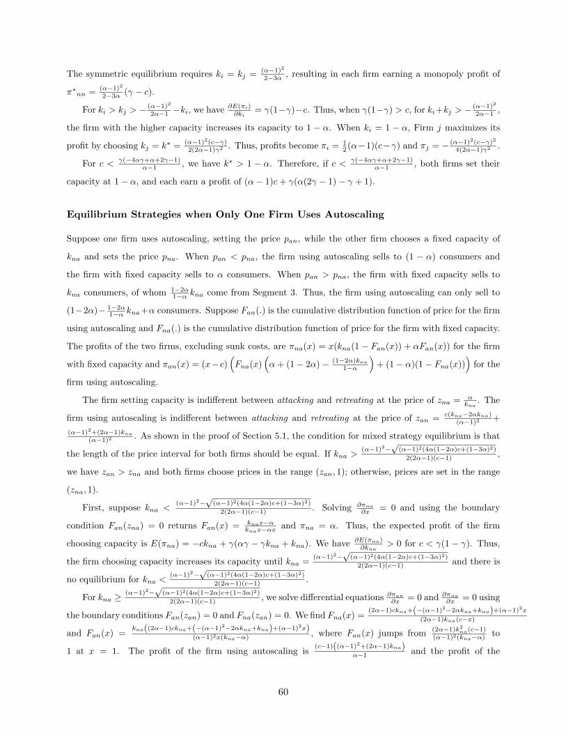
The symmetric equilibrium requires ki = kj = (α−1)2

2−3α , resulting in each firm earning a monopoly profit of

π∗nn = (α−1)2

2−3α (γ − c).

For ki > kj > − (α−1)2

2α−1 −ki, we have ∂E(πi)∂ki

= γ(1−γ)−c. Thus, when γ(1−γ) > c, for ki+kj > − (α−1)2

2α−1 ,

the firm with the higher capacity increases its capacity to 1 − α. When ki = 1 − α, Firm j maximizes its

profit by choosing kj = k∗ = (α−1)2(c−γ)2(2α−1)γ2 . Thus, profits become πi = 1

2 (α−1)(c−γ) and πj = − (α−1)2(c−γ)2

4(2α−1)γ2 .

For c < γ(−4αγ+α+2γ−1)α−1 , we have k∗ > 1 − α. Therefore, if c < γ(−4αγ+α+2γ−1)

α−1 , both firms set their

capacity at 1− α, and each earn a profit of (α− 1)c+ γ(α(2γ − 1)− γ + 1).

Equilibrium Strategies when Only One Firm Uses Autoscaling

Suppose one firm uses autoscaling, setting the price pan, while the other firm chooses a fixed capacity of

kna and sets the price pna. When pan < pna, the firm using autoscaling sells to (1 − α) consumers and

the firm with fixed capacity sells to α consumers. When pan > pna, the firm with fixed capacity sells to

kna consumers, of whom 1−2α1−α kna come from Segment 3. Thus, the firm using autoscaling can only sell to

(1−2α)− 1−2α1−α kna+α consumers. Suppose Fan(.) is the cumulative distribution function of price for the firm

using autoscaling and Fna(.) is the cumulative distribution function of price for the firm with fixed capacity.

The profits of the two firms, excluding sunk costs, are πna(x) = x(kna(1− Fan(x)) + αFan(x)) for the firm

with fixed capacity and πan(x) = (x−c)(Fna(x)

(α+ (1− 2α)− (1−2α)kna

1−α

)+ (1− α)(1− Fna(x))

)for the

firm using autoscaling.

The firm setting capacity is indifferent between attacking and retreating at the price of zna = αkna

. The

firm using autoscaling is indifferent between attacking and retreating at the price of zan = c(kna−2αkna)(α−1)2 +

(α−1)2+(2α−1)kna(α−1)2 . As shown in the proof of Section 5.1, the condition for mixed strategy equilibrium is that

the length of the price interval for both firms should be equal. If kna >(α−1)2−

√(α−1)2(4α(1−2α)c+(1−3α)2)

2(2α−1)(c−1) ,

we have zan > zna and both firms choose prices in the range (zan, 1); otherwise, prices are set in the range

(zna, 1).

First, suppose kna <(α−1)2−

√(α−1)2(4α(1−2α)c+(1−3α)2)

2(2α−1)(c−1) . Solving ∂πna∂x = 0 and using the boundary

condition Fan(zna) = 0 returns Fan(x) = knax−αknax−αx and πna = α. Thus, the expected profit of the firm

choosing capacity is E(πna) = −ckna + γ(αγ − γkna + kna). We have ∂E(πna)∂kna

> 0 for c < γ(1 − γ). Thus,

the firm choosing capacity increases its capacity until kna =(α−1)2−

√(α−1)2(4α(1−2α)c+(1−3α)2)

2(2α−1)(c−1) and there is

no equilibrium for kna <(α−1)2−

√(α−1)2(4α(1−2α)c+(1−3α)2)

2(2α−1)(c−1) .

For kna ≥(α−1)2−

√(α−1)2(4α(1−2α)c+(1−3α)2)

2(2α−1)(c−1) , we solve differential equations ∂πan∂x = 0 and ∂πna

∂x = 0 using

the boundary conditions Fan(zan) = 0 and Fna(zan) = 0. We find Fna(x) =(2α−1)ckna+(−(α−1)2−2αkna+kna)+(α−1)2x

(2α−1)kna(c−x)

and Fan(x) =kna((2α−1)ckna+(−(α−1)2−2αkna+kna)+(α−1)2x)

(α−1)2x(kna−α) , where Fan(x) jumps from(2α−1)k2na(c−1)(α−1)2(kna−α) to

1 at x = 1. The profit of the firm using autoscaling is(c−1)((α−1)2+(2α−1)kna)

α−1 and the profit of the

60

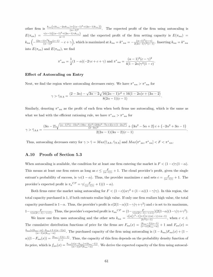
other firm iskna(c(kna−2αkna)+((α−1)2+(2α−1)kna))

(α−1)2 . The expected profit of the firm using autoscaling is

E(πan) =γ(c−1)((α−1)2+(2α−1)γkna)

α−1 and the expected profit of the firm setting capacity is E(πna) =

kna

(− (2α−1)γ2kna(c−1)

(α−1)2 − c+ γ)

, which is maximized at kna = k∗na = − (α−1)2(c−γ)2(2α−1)γ2(c−1) . Inserting kna = k∗na

into E(πan) and E(πna), we find

π∗an =1

2(1− α)(−2γc+ c+ γ) and π∗na =

(α− 1)2(c− γ)2

4(1− 2α)γ2(1− c).

Effect of Autoscaling on Entry

Next, we find the region where autoscaling decreases entry. We have π∗nn > π∗na for

γ > γNA =(2− 3α)−

√3α− 2

√16(2α− 1)c2 + 16(1− 2α)c+ (3α− 2)

8(2α− 1)(c− 1).

Similarly, denoting π∗aa as the profit of each firm when both firms use autoscaling, which is the same as

what we had with the efficient rationing rule, we have π∗nn > π∗aa for

γ > γAA =(3α− 2)

√(α−1)2((−15α2+16α−4)c2+2(6α2−7α+2)c+(1−2α)2)

(2−3α)2 +(3α2 − 5α+ 2

)c+

(−2α2 + 3α− 1

)2(2α− 1)(3α− 2)(c− 1)

.

Thus, autoscaling decreases entry for γ > γ = Max[γAA, γNA] and Max[π∗aa, π∗na] < F < π∗nn.

A.10 Proofs of Section 5.3

When autoscaling is available, the condition for at least one firm entering the market is F < (1− c)γ(1−α).

This means at least one firm enters as long as c ≤ F(α−1)γ + 1. The cloud provider’s profit, given the single

entrant’s probability of success, is γc(1− α). Thus, the provider maximizes c and sets c = F(α−1)γ + 1. The

provider’s expected profit is πaCP = γ( F

(α−1)γ + 1)(1− α).

Both firms enter the market using autoscaling for F < (1− c)(αγ2 + (1−α)(1− γ)γ). In this region, the

total capacity purchased is 1, if both entrants realize high value. If only one firm realizes high value, the total

capacity purchased is 1−α. Thus, the provider’s profit is c(2(1−α)(1−γ)γ+γ2) and c is set to its maximum,

1− Fγ(α(2γ−1)−γ+1) . Thus, the provider’s expected profit is πaa

CP = (1− Fγ(α(2γ−1)−γ+1) )(2(1−α)(1−γ)γ+γ2).

We know one firm uses autoscaling and the other sets kna =c(α(γ2−1)+1)+γ(α(−γ)+α−1)

2γ2(c−1) , when c < c.

The cumulative distribution functions of price for the firms are Fna(x) = (kna−1)(x−1)(c−x)(kna−α) + 1 and Fan(x) =

kna(c(kna−α)−kna+1+(α−1)x)(α−1)x(kna−α) . The purchased capacity of the firm using autoscaling is (1− kna)Fna(x) + (1−

α)(1−Fna(x)) = (kna−1)(c−1)x−c . Thus, the capacity of this firm depends on the probability density function of

its price, which is fan(x) = kna(c(α−kna)+(kna−1))(α−1)x2(kna−α) . We derive the expected capacity of the firm using autoscal-

61

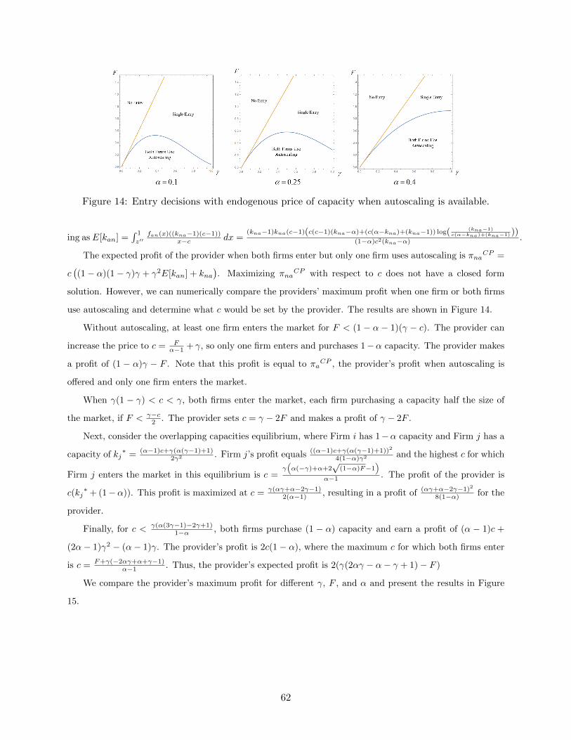
Figure 14: Entry decisions with endogenous price of capacity when autoscaling is available.

ing as E[kan] =∫ 1

z′′fan(x)((kna−1)(c−1))

x−c dx =(kna−1)kna(c−1)(c(c−1)(kna−α)+(c(α−kna)+(kna−1)) log( (kna−1)

c(α−kna)+(kna−1) ))(1−α)c2(kna−α) .

The expected profit of the provider when both firms enter but only one firm uses autoscaling is πnaCP =

c((1− α)(1− γ)γ + γ2E[kan] + kna

). Maximizing πna

CP with respect to c does not have a closed form

solution. However, we can numerically compare the providers’ maximum profit when one firm or both firms

use autoscaling and determine what c would be set by the provider. The results are shown in Figure 14.

Without autoscaling, at least one firm enters the market for F < (1 − α − 1)(γ − c). The provider can

increase the price to c = Fα−1 + γ, so only one firm enters and purchases 1−α capacity. The provider makes

a profit of (1 − α)γ − F . Note that this profit is equal to πaCP , the provider’s profit when autoscaling is

offered and only one firm enters the market.

When γ(1 − γ) < c < γ, both firms enter the market, each firm purchasing a capacity half the size of

the market, if F < γ−c2 . The provider sets c = γ − 2F and makes a profit of γ − 2F .

Next, consider the overlapping capacities equilibrium, where Firm i has 1−α capacity and Firm j has a

capacity of kj∗ = (α−1)c+γ(α(γ−1)+1)

2γ2 . Firm j’s profit equals ((α−1)c+γ(α(γ−1)+1))2

4(1−α)γ2 and the highest c for which

Firm j enters the market in this equilibrium is c =γ(α(−γ)+α+2

√(1−α)F−1

)α−1 . The profit of the provider is

c(kj∗+ (1−α)). This profit is maximized at c = γ(αγ+α−2γ−1)

2(α−1) , resulting in a profit of (αγ+α−2γ−1)2

8(1−α) for the

provider.

Finally, for c < γ(α(3γ−1)−2γ+1)1−α , both firms purchase (1 − α) capacity and earn a profit of (α − 1)c +

(2α− 1)γ2 − (α− 1)γ. The provider’s profit is 2c(1− α), where the maximum c for which both firms enter

is c = F+γ(−2αγ+α+γ−1)α−1 . Thus, the provider’s expected profit is 2(γ(2αγ − α− γ + 1)− F )

We compare the provider’s maximum profit for different γ, F , and α and present the results in Figure

15.

62

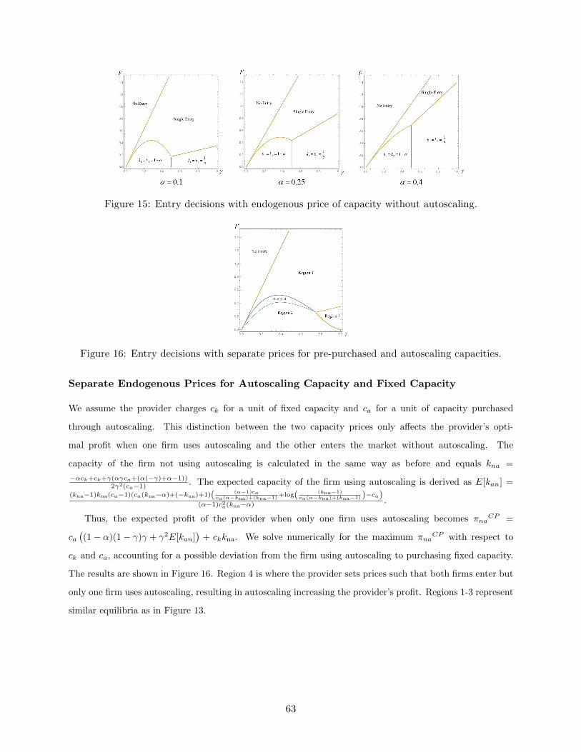
Figure 15: Entry decisions with endogenous price of capacity without autoscaling.

Figure 16: Entry decisions with separate prices for pre-purchased and autoscaling capacities.

Separate Endogenous Prices for Autoscaling Capacity and Fixed Capacity

We assume the provider charges ck for a unit of fixed capacity and ca for a unit of capacity purchased

through autoscaling. This distinction between the two capacity prices only affects the provider’s opti-

mal profit when one firm uses autoscaling and the other enters the market without autoscaling. The

capacity of the firm not using autoscaling is calculated in the same way as before and equals kna =

−αck+ck+γ(αγca+(α(−γ)+α−1))2γ2(ca−1) . The expected capacity of the firm using autoscaling is derived as E[kan] =

(kna−1)kna(ca−1)(ca(kna−α)+(−kna)+1)( (α−1)caca(α−kna)+(kna−1)

+log( (kna−1)ca(α−kna)+(kna−1) )−ca)

(α−1)c2a(kna−α) .

Thus, the expected profit of the provider when only one firm uses autoscaling becomes πnaCP =

ca((1− α)(1− γ)γ + γ2E[kan]

)+ ckkna. We solve numerically for the maximum πna

CP with respect to

ck and ca, accounting for a possible deviation from the firm using autoscaling to purchasing fixed capacity.

The results are shown in Figure 16. Region 4 is where the provider sets prices such that both firms enter but

only one firm uses autoscaling, resulting in autoscaling increasing the provider’s profit. Regions 1-3 represent

similar equilibria as in Figure 13.

63