The Doppler Method, or Radial Velocity Detection of Planets:

I. Technique

1. Keplerian Orbits

2. Spectrographs/Doppler shifts

3. Precise Radial Velocity measurements

The Doppler Effect:

The “Radial Velocity” Technique:

Johannes Kepler(1571-1630)

Three laws of planetary motion:1. Planets move in ellipses with the Sun

in on focus

2. The radius vector describes equal areasin equal times

3. The squares of the periods are to each other as the cubes of the mean distances

ap

as

V

msmp

Newton‘s form of Kepler‘s Law

28.4P1/3ms

2/3

mp sin iVobs =

Approximations:

ms » mp

Planet Mass (MJ) V(m s–1)

Mercury 1.74 × 10–4 0.008

Venus 2.56 × 10–3 0.086

Earth 3.15 × 10–3 0.089

Mars 3.38 × 10–4 0.008

Jupiter 1.0 12.4

Saturn 0.299 2.75

Uranus 0.046 0.297

Neptune 0.054 0.281

Pluto 1.74 × 10–4 3×10–5

Radial Velocity Amplitude of Sun due to Planets in the Solar System

Radial Velocity Amplitude of Planets at Different aR

adia

l Vel

ocity

(m

/s)

G2 V star

Obs

e rve

r Because you measure the radial component of the velocity you cannot be sure you are detecting a low mass object viewed almost in the orbital plane, or a high mass object viewed perpendicular to the orbital plane

We only measure MPlanet x sin i

i

Requirements:• Accuracy of better than 10 m/s• Stability for at least 10 Years

Jupiter: 12 m/s, 11 years

Saturn: 3 m/s, 30 years

Radial Velocity measurements

28.4P1/3ms

2/3

mp sin iVobs =

Radial velocity shape as a function of eccentricity:

Radial velocity shape as a function of , e = 0.7 :

Eccentric orbit can sometimes escape detection:

With poor sampling this star would be considered constant

Measurement of Doppler Shifts

In the non-relativistic case:

– 0

0

= vc

We measure v by measuring

The Radial Velocity Measurement Error with Time

How did we accomplish this?

The Answer:

1. Electronic Detectors (CCDs)

2. Large wavelength Coverage Spectrographs

3. Simultaneous Wavelength Calibration (minimize instrumental effects)

4. Fast Computers...

Instrumentation for Doppler Measurements

High Resolution Spectrographs with Large Wavelength Coverage

collimator

Echelle Spectrographs

slit

camera

detector

corrector

From telescope

Cross disperser

A spectrograph is just a camera which produces an image of the slit at the detector. The dispersing element produces images as a function of wavelength

without disperser

with disperser

slit

slit

A Spectrum Of A Star:A Spectrum Of A Star:

On a detector we only measure x- and y- positions, there is no information about wavelength. For this we need a calibration source

y

x

CCD detectors only give you x- and y- position. A doppler shift of spectral lines will appear as x

x →→ v

How large is x ?

R Ang/pixel Velocity per pixel (m/s)

pixel Shift in mm

500 000 0.005 300 0.06 0.001

200 000 0.125 750 0.027 4×10–4

100 000 0.025 1500 0.0133 2×10–4

50 000 0.050 3000 0.0067 10–4

25 000 0.10 6000 0.033 5×10–5

10 000 0.25 15000 0.00133 2×10–5

5 000 0.5 30000 6.6×10–4 10–5

1 000 2.5 150000 1.3×10–4 2×10–6

So, one should use high resolution spectrographs….up to a point

For v = 20 m/s

How does the RV precision depend on the properties of your spectrograph?

The Radial Velocity precision depends not only on the properties of the spectrograph but also on the properties of the star.

Good RV precision → cool stars of spectral type later than F6

Poor RV precision → hot stars of spectral type earlier than F6

Why?

A7 star

K0 star

Early-type stars have few spectral lines (high effective temperatures) and high rotation rates.

A0 A5 F0 F5

RV

Err

or (

m/s

)

G0 G5 K0 K5 M0

Spectral Type

Main Sequence Stars

Ideal for 3m class tel. Too faint (8m class tel.). Poor precision

98% of known exoplanets are found around stars with spectral types later than F6

Eliminate Instrumental Shifts

Recall that on a spectrograph we only measure a Doppler shift in x (pixels).

This has to be converted into a wavelength to get the radial velocity shift.

Instrumental shifts (shifts of the detector and/or optics) can introduce „Doppler shifts“ larger than the ones due to the stellar motion

Traditional method:

Observe your star→

Then your calibration source→

Problem: these are not taken at the same time…

... Short term shifts of the spectrograph can limit precision to several hunrdreds of m/s

Solution 1: Observe your calibration source (Th-Ar) simultaneously to your data:

Spectrographs: CORALIE, ELODIE, HARPS

Stellar spectrum

Thorium-Argon calibration

Solution 2: Absorption cell

a) Griffin and Griffin: Use the Earth‘s atmosphere:

O2

6300 Angstroms

Filled circles are data taken at McDonald Observatory using the telluric lines at 6300 Ang.

Example: The companion to HD 114762 using the telluric method. Best precision is 15–30 m/s

Limitations of the telluric technique:

• Limited wavelength range (≈ 10s Angstroms)

• Pressure, temperature variations in the Earth‘s atmosphere

• Winds

• Line depths of telluric lines vary with air mass

• Cannot observe a star without telluric lines which is needed in the reduction process.

Absorption lines of the star

Absorption lines of cell

Absorption lines of star + cell

b) Use a „controlled“ absorption cell

Drawbacks:• Limited wavelength range (≈ 100 A) • Temperature stablized at 100 C• Long path length (1m)• Has to be refilled every observing run• Dangerous

Campbell & Walker: Hydrogen Fluoride (HF) cell:

Demonstrated radial velocity precision of 13 m s–1 in 1980!

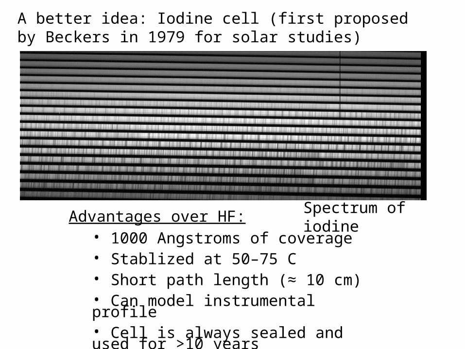
A better idea: Iodine cell (first proposed by Beckers in 1979 for solar studies)

Advantages over HF:• 1000 Angstroms of coverage• Stablized at 50–75 C• Short path length (≈ 10 cm)• Can model instrumental profile• Cell is always sealed and used for >10 years• If cell breaks you will not die!

Spectrum of iodine

HARPS

Simultaneous ThAr cannot model the IP. One has to stabilize the entire spectrograph

Barycentric Correction

Earth’s orbital motion can contribute ± 30 km/s (maximum)

Earth’s rotation can contribute ± 460 m/s (maximum)

Needed for Correct Barycentric Corrections:• Accurate coordinates of observatory

• Distance of observatory to Earth‘s center (altitude)

• Accurate position of stars, including proper motion:

′′

Worst case Scenario: Barnard‘s star

Most programs use the JPL Ephemeris which provides barycentric corrections to a few cm/s

For highest precision an exposure meter is required

time

Photons from star

Mid-point of exposure

No clouds

time

Photons from star

Centroid of intensity w/clouds

Clouds

Differential Earth Velocity:

Causes „smearing“ of spectral lines

Keep exposure times < 20-30 min